ADJUSTING FOR GEOGRAPHIC VARIATIONS IN TEACHER COMPENSATION:

UPDATING THE TEXAS COST-OF-EDUCATION INDEX Lori Taylor

Texas A&M University

Introduction

In 1999, the 76th Texas Legislature directed the Charles A. Dana Center at the

University of Texas at Austin “to conduct a study of variations in known resource costs

and costs of education beyond the control of a school district” and to “make

recommendations to the 77th Legislature as to methods of adjusting funding under

Chapter 42, Education Code, to reflect variations in resource costs and costs of

education.” The Dana Center was directed to do this work with the assistance of the

Texas Comptroller of Public Accounts, the Texas Education Agency, and Texas A&M

University. Their summary report, A Study of Uncontrollable Variations in the Costs of

Texas Public Education: A summary report prepared for the 77th Texas Legislature

(Alexander et al. 2000), explored multiple strategies for revising the Cost-of-Education

Index (CEI) to reflect the substantial changes in Texas during the 1990s. Their follow-up

Technical Supplement extended the analysis to incorporate additional information from

the 1999-2000 school year.

At the behest of the Joint Select Committee on Public School Finance, this study

further extends the Dana Center analysis of teacher compensation. As such, we

incorporate information covering five school years—1998-99, 1999-2000, 2000-01,

2001-02, and 2002-03. We also incorporate information from the 2000 Census. Our

analysis demonstrates both that there is considerable need for cost of education

adjustments in Texas and that there is a need to update the Texas CEI.

The Existing CEI

The CEI is the mechanism that Texas uses to adjust its school finance formula to

compensate for variations in labor costs that are beyond the control of school districts. As

implemented, the CEI increases the amount of state aid received by school districts in

2

high cost areas and reduces the amount of local revenue redistributed among districts

through a process known formally as recapture and informally as Robin Hood. Without

the CEI, aggregate state aid to school districts would have been 12 percent lower and

aggregate recapture payments nine percent higher during the 2002-03 school year. (For a

more complete discussion of the Texas school finance formula and the CEI, see

Appendix A.)

The CEI reflects the systematic variation in teacher salaries arising from five

factors—district size, district type, the percentage of low income students, the average

beginning teacher salary in surrounding districts, and location in a county with a

population of less than 40,000—holding constant at the mean variations in property

wealth per teacher, the total effective tax rate, the graduation rate, the percent minority

teaching staff, non-salary benefit expenditures per pupil, and teacher characteristics.1

The CEI ranges from 1.02 to 1.20, indicating that the cost of hiring a teacher in the

highest cost districts is 18 percent higher than the cost of hiring a comparable individual

in the lowest cost districts. However, the existing CEI has not been updated since its

adoption in 1991, which means that the annual distribution of approximately $1.34 billion

rests on teacher compensation patterns and school district characteristics from 1989.

The 2000 Study by the Charles A. Dana Center

The 2000 Dana Center study explored four different strategies for measuring the

cost of education: replication analysis, new compensation models, comparable wage

model cost of living, and a cost-function analysis.

The first three strategies, discussed in detail below, focus on uncontrollable

variations in the prices that districts must pay for their most important resource—

teachers. The cost-function analysis builds on the price analysis to incorporate costs that

derive from variations in the needs of students and the costs associated with being too

small to take advantage of economies of scale. Cost-function analysis is explored in more

detail in a companion report. Here we focus on variations in the price of teachers.

3

Replication Analysis

The replication analysis used the same set of controllable and uncontrollable

variables as were used to generate the existing CEI (see table 1). The researchers

deviated from the original process only when necessary to maintain correct statistical

methodology or to follow the guidelines of the current Education Code. The resulting

index values range from 1.00 to 1.23.2 As a general rule, these index values are lowest in

rural parts of the state, and highest in Houston and along the border with Mexico

New Compensation Models

Because the replication was faithful to the original specification, it relies on a very

restricted set of teacher and community characteristics. Expanding the analysis beyond

replication analysis required a new model of teacher compensation. The Dana Center

modeled teacher compensation according to the factors that influence what teachers are

willing to accept from school districts. Thus, they modeled compensation as a function of

teacher characteristics, characteristics of the working environment, and characteristics of

the community in which the school district is located. The factors included in their

preferred specification are presented in table 2.3

Measures of a district’s ability to pay are notably absent from a willingness-to-

accept model of teacher compensation. Most teachers are not willing to accept less

compensation from poor districts simply because the districts have a diminished ability to

pay. Instead, highly qualified and mobile teachers tend to accept the most attractive job

offers, and teachers with fewer options or fewer skills either accept the remaining

positions or leave the profession. Thus, the distribution of teacher characteristics varies

according to each districts’ ability to pay, but the salary of a teacher with given

characteristics does not.

A Teacher Salary Index was constructed by predicting the salary that would be

demanded by the typical Texas teacher from each district. Thus, the models were

evaluated using the state average for personnel characteristics, the school district average

for district-level characteristics, and the metropolitan area (urban) or county (rural)

4

average for all other characteristics. Predicted salaries below the state minimum were

assigned the state minimum. A district’s index value is the district’s predicted salary

divided by the minimum predicted salary in the state (which in this case is the state

minimum). In addition, the index is adjusted upward by 6.2 percent to reflect the

employer’s contribution in the 14 districts where teachers participate in the Social

Security system.

The teacher salary index ranges from 1.00 to 1.28, with large districts that

participate in the Social Security system receiving the highest values. As a general rule,

index values are highest along the Gulf Coast and along the border with Mexico and are

lowest in small urban areas like San Angelo and Sherman.

Because surveys suggest that the benefits teachers receive from school districts

vary greatly across the state, the Dana Center researchers also estimated a salary and

benefits version of their compensation model. The researchers used a survey by the

Texas State Teachers Association (TSTA) to estimate the average cost of health

insurance benefits received by teachers in each district, adjusted salaries upward by that

amount, and re-estimated the models. The researchers found that the basic pattern of

salaries is not sensitive to the inclusion or exclusion of benefits. However, the minimum

wage limits the variation of the Salary Index while it has no such effect on the Salary and

Benefits Index. As a consequence, the Salary and Benefits Index covers a greater range—

from 1.00-1.34.

A Comparable Wage Model of Cost-of-Living

Both the replication analysis and the new compensation models use the pattern of

teacher salaries to identify uncontrollable variations in labor costs. The Comparable

Wage model uses the pattern of non-educator salaries to accomplish the same goal.

Underlying the Comparable-Wage model is the observation that school districts are not

the only businesses that must cope with regional variations in the wages that their

employees demand. Like educators, bank tellers, nurses, and accountants will all demand

higher wages in areas with higher costs of living. Therefore, systematic regional

variations in the wages paid to comparable professionals should reflect variations in the

5

cost of living that can be used to predict systematic variations in the wages paid to

educators.

The Dana Center researchers used regression analysis to estimate local wage

levels from earnings data provided by the Texas Workforce Commission (TWC). Their

analysis of wages in the financial and services industries yielded a cost-of-living index

that ranged from 1.00 to 1.94. The index was highest in the major urban areas and lowest

in rural Texas.

The 2004 Study for the Joint Select Committee

This analysis for the Joint Select Committee follows the general structure of the

original Dana Center report, but focuses exclusively on the new compensation models

and an alternative version of the comparable wage model. The primary contributions of

this analysis arise from the incorporation of revised and newly available data and the

extension of the analysis to cover multiple years.

Newly Available Data

Another three years of teacher compensation data are now available. Whereas the

original Dana Center report focused on the 1998-99 school year, and the technical

supplement covered 1999-2000, we now have access to data on the 2000-01, 2001-02,

and 2002-03 school years.

We also have access to data unavailable during the prior analyses. In particular,

the State Board of Educator Certification has provided us with a measure of the time each

individual spends teaching in a field for which he or she is certified. Thus, we now know

that most teachers are fully certified in the subjects they teach, but that on average Texas

teachers spend more than 25 percent of their teaching time in a field for which they are

not certified. One would expect that a fully certified teacher would be more attractive to

potential employers and thus able to command a wage premium. On the other hand,

teachers may find it burdensome to teach outside of their fields and require a premium to

do so. In either case, this indicator allows us to more fully capture teacher qualifications

and working conditions.

6

We have new data from the 2000 Census. These data support an alternative

Comparable Wage Index that is based on the individual earnings of college graduates in

Texas.

Finally and crucially, we have new measures of labor market areas. The United

States Office of Management and Budget (OMB) used information on population density

and commuting patterns from the 2000 Census to substantially revise its definition of

labor market areas in Texas. According to the OMB, there are now three types of labor

markets in Texas: metropolitan statistical areas (MSAs), micropolitan statistical areas

(MCSAs) and counties. The newly designated MCSAs represent a common labor market

centered on a town of moderate size that is not part of a metropolitan area (Nacogdoches

or Granbury for example).

Twenty-two formerly rural counties are now part of metropolitan areas. Harrison,

Henderson, and Hood counties are no longer part of a metropolitan area, although each is

part of a micropolitan area. The Midland-Odessa metropolitan area has been separated

into two distinct MSAs (Midland and Odessa), while the Brazoria and Galveston

metropolitan areas have been folded into the massive Houston-Baytown-Sugar Land

Metropolitan area.

Analysis on the basis of these revised definitions should give a more accurate

picture of labor market conditions in Texas. Therefore, we have used these new

definitions to revise our measures of community characteristics and distance to the center

of the nearest MSA.4 For the 423 traditional school districts in a metropolitan area, the

community is the MSA; for the 187 districts in a micropolitan area, the community is the

MCSA. For rural districts, the community is the county in which the school district is

located.

Updating the Models of Teacher Compensation

As a first pass at the data, we re-estimated the Salary Index and the Salary and

Benefits Index for each school year from 1998-99 through 2002-03.5 The analysis uses

revised measures of the same environmental factors and teacher characteristics as in the

original Dana Center Report (see table 2), plus our new indicator of the percent of time

individuals spend teaching in their field of certification and a new indicator for location

7

in a micropolitan statistical area. (For more information on revisions to the data, see

Appendix B.) The specification has also been modified to allow the relationship between

teacher compensation and urban housing values to be a function of the distance from the

center of the metropolitan area. This more general specification should allow a tighter fit

to the compensation data. As with the earlier Dana Center analysis, we estimate separate

models for urban and rural school districts.

The estimation yields reasonable results about the impact on compensation of

teacher characteristics and environmental factors. As one would expect, teacher

compensation increases with experience and educational attainment. All other things

being equal, teachers demand a premium to teach in sparsely populated areas and areas

with relatively high housing costs. Interestingly, we find a weak negative relationship

between time-in-field and teacher compensation. Apparently, the premium that teachers

require to take on the additional work of teaching outside their field more than offsets the

premium teachers require for being fully certified.

Index values for each year were constructed by predicting the compensation

(either salary or salary and benefits) that would be demanded from each district by the

typical Texas teacher, if that teacher were fully certified in the subjects he or she was

teaching.6 In evaluating the index, we use three-year moving averages for all district and

community characteristics to limit the influence of one-time events and temporary

situations. Given concerns that the share of mainstreamed special education students is

more properly viewed as a factor within school district control, we treat it as such in the

construction of index values for this report. (A version of the index values presuming

that the share of mainstreamed special education students is outside of district control

will follow in a technical supplement.) In contrast with the Dana Center Study, the index

values are not adjusted to reflect a district’s participation in the Social Security system,

although such adjustments could be made should the Legislature so desire. (Again, a

version of the index that incorporates such adjustments will follow in a technical

supplement.)

Predicted salaries below the state minimum were assigned the state minimum. A

district’s index value is the district’s predicted salary divided by the minimum predicted

salary in the state.

8

The resulting index values are very well correlated with one another across time.

Table 3 presents the correlations among the various indexes. The upper panel illustrates

the year-by-year correlations among the Salary Indexes. The middle panel illustrates the

correlations among the Salary and Benefits Indexes, and the bottom panel indicates the

correlation between each Salary Index and its Salary and Benefits Index counterpart.

Values above the diagonal in panels 1 and 2 indicate the correlations for urban districts;

values below the diagonal indicate the correlations for rural districts. A correlation

coefficient of 1.00 indicates that two index values move together perfectly.

As in the original Dana Center report, we find a strong correspondence between

the Salary and Benefits Index in any given year and the Salary Index for that same year.

The two indexes are nearly perfectly correlated in urban areas and very highly correlated

in rural areas. The inclusion of health care benefits tends to dampen the impact of

housing costs and student characteristics on the rural index. Figure 1 illustrates the

relationship between the Salary Index and the Salary and Benefits Index for 2003.

The consistency across index values is particularly striking given the changes in

Texas during the last five years. The analysis straddles a recession that hit some parts of

the state harder than others and particularly affected labor markets in Dallas and Austin.

The average value of single-family homes fell in a handful of markets while it rose more

than 40 percent in at least as many others. Meanwhile in the classroom, more and more

districts found themselves coping with the challenges of immigrant students and limited

English proficient (LEP) students. In 1999, only 120 Texas districts had more than one

percent immigrant students; by 2003 that count had risen to 255 districts. In 2003, 838

Texas school districts had more than one percent LEP students, up from 766 districts in

1999.

Changes in education policy also stirred up the teacher market between 1999 and

2003. Late in the spring of 1999, the 76th Texas Legislature mandated a teacher salary

increase, effective for the 1999-2000 school year. Districts were required to increase

annual compensation for all full-time teachers by $3,000 and to layer this raise on top of

any previously announced salary increase. Then, for 2003, the 77th Texas Legislature

funded a $1,000 pay supplement for all full-time teachers and required districts to

contribute at least $1,800 toward health care coverage. Unanticipated changes in the

9

salary scale and unfamiliarity with accounting for the supplement introduced noise into

the payroll files for 2000 and 2003, and therefore reduced the accuracy of the estimation

for those years.

Changes in the salary structure for teachers had a particular impact on the salary

indexes. In 1999 and 2000, more than 17 percent of the teachers in our rural sample

earned the statutory minimum. That level fell to 10 percent in 2003, even though the

$1,000 supplement instituted that year could not be used to meet the minimum

requirements. As a consequence of the rising salary structure, substantially fewer rural

school districts had predicted salaries below the state mandated minimum salary schedule

(and thus Salary Index values equal to 1.0) in 2003.

Finally, year-to-year differences in the available data on health care benefits had

an impact on the Salary and Benefits Indexes. Data on health insurance benefits come

from surveys by the Texas Retirement System (TRS) and TSTA.7 The surveys offer

more complete data coverage in some years than in others. Only 87 percent of the urban

teachers and 72 percent of the rural teachers in our salary analysis for 2001 could be

included in the salary and benefits analysis for 2001.8 Only 90 percent of the urban

teachers and 92 percent of the rural teachers could be included in our salary and benefits

analysis for 2003. In 1999, 2000, and 2002, we were able to retain more than 98.5

percent of urban teachers and 97 percent of rural teachers. The comparatively low

correlation between the Salary Index and the Salary and Benefits Index for rural districts

in 2001 likely reflects the unusually high proportion of districts for which we lack

benefits information that year and the resulting difference between districts included in

the salary estimation and districts included in the salary and benefits estimation.

Pooled Estimation of Teacher Compensation

When appropriate, pooling data across multiple years can increase the precision

with which the models are estimated and reduce the influence of one-time, transitory

effects. Given the strong correlation among index values, pooling appears reasonable.

However, examination of the coefficient values suggests that the earnings/experience

profile was noticeably flatter after the Legislature instituted its $3,000 across-the-board

10

increase in the minimum salary scale. Therefore, we estimated a pooled model that

combines the data for the four years since the policy change.9

Figure 2 illustrates the relationship between the annual Salary and Benefits Index

and the Pooled Salary and Benefits Index for 2003. As the figure illustrates, the two

indexes are highly correlated. (The correlation coefficient is .9921 for urban districts and

.9498 for rural districts.)

While the two indexes are highly correlated, there are significant differences for

specific districts. Pooling tends to moderate the index values for urban districts, pulling

up low index values and pulling down high ones. It generates systematically lower index

values for rural districts. In particular, pooling the data from multiple years leads to lower

index values for large districts and districts in major metropolitan areas.

Teacher Fixed Effects

One persistent concern is the degree to which the analysis successfully controls

for variations in teacher quality. Despite a researcher’s best efforts, there will always be

potentially important teacher characteristics that cannot be included in a statistical model.

If those omitted characteristics are correlated with the uncontrollable cost factors, then

the index can wind up misinterpreting high spending districts as high cost districts and

low spending districts as low cost districts.

One way to address this concern is to allow for teacher fixed effects. The fixed

effects methodology removes from the index any variation that might arise from

persistent teacher characteristics such as intelligence or communications skills.

Unfortunately, in so doing it also removes much of the variation that is driven by stable

characteristics of school districts. Stable district characteristics—such as geographic

remoteness—will only register for teachers who change districts. If teachers who change

districts are not representative of the teaching population as a whole, the fixed-effects

index can be misleading.

As with the pooling analysis, we estimate a teacher fixed effects model of salary

and benefits using data for the four years since 1999.10 Figure 3 illustrates the

relationship between the Teacher Fixed Effects Salary and Benefits Index for 2003 and

the Pooled Salary and Benefits Index for 2003. As the figure illustrates, the two index

11

values are highly correlated, but compared to the simple pooling model, the fixed-effects

model tends to dampen the impact of the uncontrollable cost factors in urban areas and

amplify their impact in rural areas. The fixed effects model yields index values that are

somewhat lower in major urban areas and substantially lower in Brownsville, Laredo, and

McAllen.

Choosing a Preferred Model of Teacher Compensation

Arguably, any of the estimation strategies discussed above could generate a viable

index of teacher compensation for Texas. A version of the Salary and Benefits Index has

strong intuitive appeal because it captures more of the compensation package than just

salary. On the other hand, the Salary Index draws on data from the full population of

Texas school districts rather than just those that responded to benefits surveys. In years

with near perfect coverage from the benefits surveys (1999, 2000, and 2002) the

advantages of the Salary and Benefits Index clearly outweigh the risks. In other years,

however, the choice is less clear. In particular, problems could arise from relying too

heavily on the benefits data for 2003, given the difficulties created by incomplete survey

coverage and imprecise measures of health insurance benefits arising from the

introduction of the TRS ActiveCare system (a statewide program of healthcare benefits

for employees of small school districts).

Pooling the data—with or without teacher fixed effects—reduces the risks

associated with year-specific measurement errors or selection biases. It also generates

index values that reflect only persistent relationships between compensation and cost

factors. For these reasons, we favor using a multi-year model of salary and benefits.

A comparison between the Pooled Salary and Benefits Index and the Teacher

Fixed Effects Salary and Benefits Index suggests that although the two indexes cover a

comparable range (1 to 1.30 for the Pooled, 1 to 1.29 for the Teacher Fixed Effects) the

index values of specific districts are sensitive to the choice of multi-year modeling

strategy. Differences arise either because there are unobservable aspects of teacher

quality that are correlated with the cost factors (so that unobservable quality is higher in

areas with lower housing prices or in areas with more LEP students) or because the cost

12

factors are essentially fixed in nature (so that estimated costs are dominated by the

preferences of teachers who change districts).

A Census-based Measure of Comparable Wages

One drawback to the Dana Center’s analysis of comparable wages is the lack of

information on worker characteristics. Thus, while the fine level of industrial detail in

the TWC data ensures that workers have very similar jobs, it cannot guarantee that they

have similar qualifications or demographic characteristics. As a consequence, a

community in which wages are generally low because most workers are young and

poorly educated receives the same index value as one in which wages are generally low

because the cost of living is low.

The 2000 Census provides the data needed for a comparable wage analysis.11 The

data indicate wage and salary earnings for individuals, together with not only their

occupation but also their age, gender, and educational attainment. One can be reasonably

confident that a Comparable Wage Index based on such data is not contaminated by

demographic considerations. Furthermore, by restricting the analysis to college

graduates, we can generate a wage index for non-educators who are directly comparable

to teachers.

Unfortunately, the wealth of demographic information comes at the expense of

considerable geographic detail. The only locational information on the individual Census

files is a “place of work area.” Once we consolidate any such areas that are fully

contained within a single labor market (such as combining the areas within Dallas,

Collin, and Denton counties into a single area) we are left with 51 place-of-work areas in

Texas. Most metropolitan areas have their own place-of-work area, but rural counties

areas tend to be clustered together. While the Bureau of Labor Statistics (BLS)

recognizes 23 labor markets in the Texas Panhandle (Amarillo and 22 county labor

markets), there are only two Census place-of-work areas—Amarillo and not Amarillo.

We used regression analysis to estimate the local wage level in each place-of-

work area, controlling for the age, gender, ethnicity, educational attainment, amount of

time worked, and occupation of each of the 65,656 employed, college-educated Texans in

the sample.12 Dividing the local wage level by the lowest estimated wage level yields a

13

Census-based Comparable Wage Index.13 The Census-based Comparable Wage Index

ranges from 1.00 in much of rural Texas to 1.36 in the Dallas metropolitan area.14

The Census-based Comparable Wage Index shows substantially less variation

than the Comparable Wage Index based on the TWC industry data. However, the

Census-based index also reflects substantially less geographic detail. To get a feel for

how much information is lost by aggregating the data, we re-estimated the TWC index

using Census place-of-work areas rather than BLS labor market areas. Reducing the

number of markets narrows the range on the TWC-based Comparable Wage Index.

While the original index ranged from 1.00 to 1.94, the geographically-restrained index

ranges from 1.00 to 1.71. This narrowing suggests that the Census-based Comparable

Wage Index would cover a greater range if it had greater geographic detail, implying that

the Comparable Wage Index understates differences in the cost of living in Texas.

Comparable Wages and Teacher Compensation

Table 4 presents the correlations between the Census-based Comparable Wage

Index and the two preferred indexes of teacher compensation, the Pooled Salary and

Benefits Index and the Teacher Fixed Effects Index. As the table illustrates, there is

virtually no relationship in rural areas between a wage index based on educator wages

and an index based on comparable non-educators.

The wage indexes are moderately well correlated in urban Texas, but again the

relationship is not especially close. Figure 4 illustrates the relationship between the

Comparable Wage Index and the Teacher Fixed Effects Index. (The Pooled Salary and

Benefits Index tells a similar story.) Each box represents a school district, and each row

represents a different place-of-work area. Thus, the figure indicates that where the index

based on non-educator wages is 1.36 for all school districts in the Dallas metropolitan

area, the index based on educator wages ranges from a low of 1.06 to a high of 1.27. If

we consider pupil-weighted average index values for each metropolitan area, the

Comparable Wage Index is more than 10 percentage points below both the Pooled Salary

and Benefits Index and the Fixed Effects Index in Abilene, Brownsville, El Paso, Laredo,

McAllen, and Wichita Falls.

14

Strengths and Weaknesses of the Approaches

There is no “best” approach to estimating uncontrollable variations in the price of

labor. Each approach has advantages and disadvantages.

The principal advantage of a Comparable Wage Index is that it avoids the difficult

problems associated with distinguishing variations in school district expenditures that are

controllable from those that are uncontrollable. After all, it is unlikely that school districts

will be able to manipulate the general labor market. As a cost-of-living index, the

Comparable Wage Index is also the index most similar to the education cost indexing

strategies used in other states.

The major disadvantages of any Comparable Wage Index are twofold. First, the

Comparable Wage Index may not adequately reflect the actual cost of living for school

personnel if the comparable population differs substantially from the educator population

in terms of age, educational background, or tastes for local amenities. Second, as with

any cost-of-living index, the Comparable Wage Index cannot pick up district-level

variations in the price of labor. Every school district in a labor market receives the same

index value as every other district in the market. Therefore, cost-of-living strategies

generate the same index value for an advantaged school district as for its disadvantaged

cross-town rival. By focusing on college graduates and controlling for demographic and

occupational characteristics, the Census-based Comparable Wage Index largely addresses

the first concern. However, the level of geographic aggregation makes it particularly

vulnerable to the second concern.

In contrast to the Comparable Wage Index, both of the teacher compensation

indexes are drawn from the individual salary records of Texas school districts and do a

good job of differentiating costs within labor markets. The models upon which they are

based explain more than 90 percent of the variation in teacher compensation and are

consistent with reasonable expectations about teacher compensation. For example, all

other things being equal, costs are higher in areas where housing costs are higher and in

sparsely populated areas. Costs fall as distance to a major urban area increases, but rise

as one gets farther away from continuing education opportunities for teachers. Costs tend

to rise with district size, but the independent effect of size tops out at an enrollment of

15

25,000. Costs increase with increases in the percentage of students who are immigrants

and, at least in the Pooled Salary and Benefits model, with increases in the percentage of

LEP students.

However, cost-of-education indexes that are drawn from school district

expenditures force researchers to use statistical techniques to distinguish between

controllable and uncontrollable costs. Such distinctions are inherently subject to

criticism. In this analysis, the specified student and community characteristics are all

treated as uncontrollable factors, and all other factors that influence salaries and

expenditures—including any relevant omitted factors—are treated as controllable factors.

The potential for omitting relevant factors is an important disadvantage because

significant omissions could bias the resulting index values. Scholars have expressed

particular concerns that even a broad array of observable teacher characteristics cannot

fully capture variations in teacher training, professional qualifications, or classroom

effectiveness.15

Relying on the Teacher Fixed Effects Index rather than the Pooled Salary and

Benefits Index largely addresses concerns about omitted teacher characteristics. The

fixed effects technique removes from the index any variations in compensation that arise

from persistent teacher characteristics. However, it may also strip from the index much

of the information about quasi-fixed district characteristics like a relatively low cost of

living. Choosing between the two indexes of teacher compensation involves choosing

which type of errors one can live with—underestimating the impact of controllable cost

factors or underestimating the impact of uncontrollable cost factors.

Conclusions

Our analysis of educator and non-educator wages in Texas strongly suggests that

school districts face substantial and uncontrollable differences in the price of their most

important input—teachers. By the most conservative estimate, the highest cost district

must pay 29 percent more than the lowest cost districts to hire a comparable individual.

A Census-based Comparable Wage Index suggests that the highest cost districts must pay

36 percent more than the lowest cost districts in the state. The Census-based index

16

implies that variations in the price of teachers are double those reflected in the existing

CEI and the Texas school finance formula.

Not only have uncontrollable price variations grown larger in the dozen years

since the CEI was first adopted, but the pattern of cost has shifted. Hiring costs have

risen much more rapidly in some areas than in others, changing the relative index values

of school districts. Where cost increases have been unusually large, updating revises

index values upward; where cost increases have been relatively modest, updating revises

index values downward. In rural Texas, the cost structure has changed so much that the

existing CEI can explain only a quarter of the variation in any of the indexes presented in

this report.

Updating would substantially increase the index values for major urban areas,

while generally reducing the index values for rural areas.16 Districts in the San Antonio

and Austin metropolitan areas particularly benefit from updating the CEI.

Much has changed in Texas since 1989. As a result, the existing CEI has become

badly outdated. Regardless of the updating strategy chosen by the legislature, accurately

reflecting uncontrollable variations in the cost of education requires adoption of a new

CEI.

17

Table 1: The Replication Analysis

Controllable factors (or factors adjusted for elsewhere in the

finance formula)

Uncontrollable factors

District level • Property wealth per teacher • Total effective tax rate • Graduation rate • Percent minority teaching staff • Non-salary benefit expenditures per

pupil

Teacher level • Advanced degree indicator • High School assignment indicator • Total years of teaching experience

District level • Competitive beginning average teacher

salary • Location in a county with fewer than

40,000 people • Percent low-income pupils • District type • District size in terms of students in

Average Daily Attendance (ADA)

18

Table 2: The New Compensation Analysis

Teacher characteristics Environmental factors

Individual level:

• Total years of teaching experience • Educational attainment • Gender and ethnicity • Effective days worked • Teaching assignment • Certification status • Indicator for whether the teacher was:

Assigned administrative duties

Assigned to multiple campuses

A secondary school teacher

New to the district

District level:

• Average Daily Attendance • Distance to nearest teacher certifying

institution • Distance to nearest metropolitan area • Indicator for participation in Social

Security • Percent of students who were:

Immigrants

Limited English proficient

Mainstreamed Special Education

Community level:

• Average house price • Average cooling degree days • Unemployment rate • Population density

19

Table 3: Correlations between Annual Index Values

Annual Correlation between Teacher Salary Indexes

Urban School Districts

1999 2000 2001 2002 2003

1999 0.9933 0.9691 0.9624 0.9467

2000 0.9840 0.9691 0.9610 0.9390

2001 0.9460 0.9555 0.9967 0.9854

2002 0.9299 0.9356 0.9822 0.9919

Rural School Districts

2003 0.8937 0.9017 0.9574 0.9731

Annual Correlation Between Teacher Salary and Benefits Indexes

Urban School Districts

1999 2000 2001 2002 2003

1999 0.9909 0.9747 0.9599 0.9620

2000 0.9867 0.9669 0.9446 0.9430

2001 0.9037 0.9071 0.9928 0.9830

2002 0.9549 0.9449 0.9339 0.9912

Rural School Districts

2003 0.8235 0.8304 0.8682 0.9202

Annual Correlation Between Teacher Salary Index and Salary and Benefits Index

1999 2000 2001 2002 2003

Urban School Districts 0.9878 0.9906 0.9925 0.9879 0.9933

Rural School Districts 0.9464 0.9548 0.9296 0.9564 0.9817

20

Table 4: Correlation Between Comparable Wages and Teacher Compensation Indexes

Urban School Districts Comparable

Wage Index Pooled Salary and Benefits

Index

Teacher Fixed Effects Index

Comparable Wage Index

.5028 .5697

Pooled Salary and Benefits Index

-0.1013 .9919

Rural School Districts Teacher Fixed

Effects Index .0571 .8567

21

Figure 1

Comparing the Salary Index and the Salary and Benefits Index for 2003

1

1.05

1.1

1.15

1.2

1.25

1.3

1.35

1.4

1 1.05 1.1 1.15 1.2 1.25 1.3 1.35 1.4

Annual Salary Index 2003

Ann

ual S

alar

y an

d B

enef

its In

dex

2003

urban school districtsrural school districts45 degree line

22

Figure 2

Comparing the Pooled Index to the Annual Index

1

1.05

1.1

1.15

1.2

1.25

1.3

1.35

1.4

1 1.05 1.1 1.15 1.2 1.25 1.3 1.35 1.4

Annual Salary and Benefits Index 2003

Pool

ed S

alar

y an

d B

enef

its In

dex

2003

urban school districtsrural school districts45 degree line

23

Figure 3

Comparing the Teacher Fixed Effects Index to the Pooled Index

1

1.05

1.1

1.15

1.2

1.25

1.3

1.35

1.4

1 1.05 1.1 1.15 1.2 1.25 1.3 1.35 1.4

Pooled Salary and Benefits Index 2003

Tea

cher

Fix

ed E

ffec

ts S

alar

y an

d B

enef

its In

dex

2003

urban school districtsrural school districtsBrownsville, Laredo & McAllen45 degree line

24

Figure 4

The Variation of Teacher Compensation within Cities

0.95

1

1.05

1.1

1.15

1.2

1.25

1.3

1.35

1.4

1 1.05 1.1 1.15 1.2 1.25 1.3 1.35 1.4

Teacher Fixed Effects Salary and Benefits Index 2003

Com

para

ble

Wag

e In

dex

Dallas

Houston

Fort WorthAustin

25

Notes

1 For districts with average daily attendance between 1,600 and 2,000 students, an adjusted CEI is used. The adjusted CEI = CEI × (1.0 + ((2000 – ADA) × .00014)) 2 It is important to note that the updated version of the existing CEI generates predicted teacher salaries below the state minimum salary scale for at least some teachers in 303 Texas districts. For consistency with the existing CEI, this pattern was ignored in the construction of the index. 3 The analysis was generally insensitive to the inclusion of additional district and community factors. See A Study of Uncontrollable Variations in the Costs of Texas Public Education: A summary report prepared for the 77th Texas Legislature Alexander et al. (2000). 4 Data on unemployment rates will not be available according to the new definitions until 2005. Therefore, the unemployment rate variable continues to use the 1990 labor market definitions. 5 In this analysis, we implicitly assume that teachers receive $100 in value from a health insurance benefit for which the district pays $100. This assumption may not be accurate, given that large numbers of teachers chose not to participate in the health plans offered to them by districts. 6 In this context, the typical Texas teacher has the average characteristics of the individuals for whom we have complete data who were full-time teachers in traditional public school districts during the 2002-03 school year. Thus, each year the models were evaluated using the 2003 state average for personnel characteristics, except that the indicator for fully certified is set equal to one, and the time in field of certification is set equal to one hundred percent. 7 In each year, we rely on the benefits survey that provides information on the greatest proportion of Texas teachers. Benefits data for 2000 and 2002 come from TRS. The benefits data for odd-numbered years come from TSTA. The two surveys reflect slightly different definitions of benefits. For TRS data, we define the value of health insurance benefits received by teachers as the maximum district outlay for single coverage; for TSTA data, we define the value of benefits as the most common district outlay for single coverage. Analysis of a year for which we have good coverage for both sources of information (1999) suggests that the Salary and Benefits estimation is not sensitive to the differences between the two surveys. The correlation between the TRS-based and TSTA-based versions of the Salary and Benefits Index for 1999 is .997 for urban districts and .992 for rural districts.

The introduction of the TRS ActiveCare program created a discontinuity in the TSTA survey for 2002-03. ActiveCare is a statewide healthcare benefits program for school district employees. Only districts that indicated they did not intend to participate in ActiveCare were asked to complete the survey. For survey participants, the annual healthcare benefit per teacher comes from the survey responses. For districts that participated in the TRS ActiveCare program during any part of 2002-2003, the annual healthcare benefit received by teachers is presumed to be $1,800 (the minimum monthly contributions for health care coverage under HB 3343). A survey by 858 Texas school districts conducted by TRS in November and December of 2002 indicated that 59 percent of districts contribute exactly the minimum required by law ($1,800 per year) while 40 percent contributed more than required by law. Assuming that ActiveCare participants contribute only the minimum required by law clearly underestimates the benefits provided by a significant proportion of districts (only 21 percent of the districts in our analysis have benefits above the legal minimum in 2003) but we lack reliable information as to which ActiveCare districts are providing more than $1,800 per year. 8 Although Houston ISD and Dallas ISD did not respond to the TSTA survey, they graciously provided answers to the survey questions for this analysis. We are grateful for their assistance. 9 Arguably, we should use random effects estimation to capture the possible correlation among errors for a specific individual. The large number of individuals makes the computational cost of such estimation prohibitive.

26

10 The model excludes individual teacher characteristics that lack cross-sectional variation in a fixed-effect specification. Such variables include sex, ethnicity and years of experience. 11 The data come from the 5-Percent Public Use Microdata sample. 12 We exclude self-employed workers, workers without a college degree, those who work less than half time or for less than $5,000 per year, and anyone who has a teaching occupation or who is employed in the elementary and secondary education industry. We control for occupation rather than industry because the Census provides more occupational detail than industrial detail. 13 Actually, we divide by a reference wage that is the lowest estimated wage, adjusted for measurement error. We add two standard errors to the least squares mean wage in each place of work area. The reference wage is the lowest error-adjusted wage. No place of work area has an estimated wage that is significantly lower than this reference wage. 14 Although the Census assigns some of the counties from Texas major metropolitan areas to “place of work areas” outside their MSA, we assign the metropolitan area wage index to all counties in the metropolitan area. 15 See, for example, Dan D. Goldhaber, “An Alternative Measure of Inflation in Teacher Salaries” in Selected Papers in School Finance, 1997, ed. William J. Fowler, Jr. (Washington, D.C.: U.S. Department of Education, National Center for Education Statistics). 16 Updating also generates index values that differ markedly from those estimated in the previous Dana Center reports. The redefinition of labor market areas is largely responsible for the differences, but housing appreciation also plays a role. Over the last three years, the assessed value of single-family homes increased by 20 percent for the average urban district, but only 13 percent for the average rural district. A rising cost-of-living has shifted urban salaries upward more rapidly than rural salaries, thereby raising urban index values and lowering rural ones.

Appendix A The Existing Texas Cost-of-Education Index

Elements Of The Existing CEI

The existing Cost-of-Education Index is composed of two parts: (1) a price component

which attempts to compensate for regional variations in resource costs and the costs of

education and (2) a scale component which addresses higher costs associated with

providing educational services in districts with student populations between 1,600 and

2,000.

The Price Component of the CEI (TAC § 203.10)

The price component of the CEI is designed to adjust for variations in teacher payroll

costs that are beyond the control of school districts. Legislative Education Board

researchers used multiple regression analysis17 to assess the impact of certain controllable

and uncontrollable factors on the predicted salary of a teacher. The explanatory factors

that were included in this analysis are presented in Figure A1.

Figure A1 Controllable and Uncontrollable Factors Included in Calculation of the

Price Component of the CEI

Controllable factors (or factors adjusted for elsewhere in the Foundation School Program) Uncontrollable factors

District level: • Property wealth per teacher • Total effective tax rate • Graduation rate • Percent minority teaching staff • Non-salary benefit expenditures per pupil

Teacher level: • Whether the teacher has an advanced degree • Whether the teacher is assigned to grades 7–12 • Total years of teaching experience

District level: • Competitive beginning average teacher

salary • Location in a county with fewer than 40,000

people • Percent low-income pupils • District type • District size in terms of students in Average

Daily Attendance (ADA)

The 1990 regression model that was used to isolate uncontrollable price variations

identified five factors that were found to have an impact on teacher salaries: average

beginning teacher salary in contiguous counties, location in a rural county (less than

40,000 population), percent low-income students, district type (suburban, independent

28

town, or rural), and district size in terms of student population. To determine an index,

they calculated the independent impact of each of these uncontrollable factors on the

predicted salary of a teacher when all other factors were held constant. For example, they

analyzed how variations in the percentage of low-income students in a school district

caused predicted teacher salaries to change when all other factors remained constant.

Figure A2 was constructed for developing the price component, based on the results of

the regression analysis.

Figure A2 The Price Component of the CEI

Amount to add to 1.00

Competitive beginning average

teacher salary

County population less than 40,000?

District type

Percent low income

students Average Daily Attendance (ADA)

-0.01 Independent Town

.00 Below $17,300 No Below 50% 200 to 499

.01 $17,300 to $17,750 Yes Rural 50 - < 68% 500 to 999 or < 200

.02 $17,751 to $18,250 68 - < 77% 1000 to 1,599

.03 $18,251 to $18,700 77 - < 86% 1,600 to 2,399

.04 $18,701 to $19,100 86 - < 93% 2,400 to 3,599

.05 $19,101 to $19,500 93% or more 3,600 to 5,399

.06 $19,501 to $20,000 5,400 to 8,499

.07 $20,001 to $20,450 8,500 or more

.08 $20,451 to $20,850

.09 $20,851 or more

Competitive beginning average teacher salary for a district is the average annual salary of beginning instructional personnel for all other districts in the same county as the district and all districts in counties contiguous to the district’s county.

A district classified as an Independent Town is the largest school district in a county with a population of 25,000 to 100,000, or any other district in that county with an ADA of at least 75 percent of the largest district’s ADA. Furthermore, the district must not be able to be classified by the Texas Education Agency as a major suburban district or another central city suburban district. Districts classified as Rural either have between 300 and 743 students in ADA and a growth rate of less than 20 percent or have less than 300 students in ADA.

Figure A3 illustrates how the price component of the 1991 CEI was calculated for

Abilene ISD, Austin ISD, Brownsville ISD, and Hale Center ISD. Note how a high

competitive beginning average teacher salary, a larger percentage of low-income

29

students, and a large district size in terms of average daily attendance results in a

relatively higher CEI for Brownsville.

Figure A3 Sample Price Component Calculations

District

1989-1990 Competitive beginning average

teacher salary

County population less than 40,000?

Independent Town or Rural?

Percent low

income students ADA

CEI value

Abilene ISD $18,052 No No 41.54 17,466 1.09

Austin ISD $18,696 No No 40.01 61,745 1.10

Brownsville ISD $21,222 No No 80.76 38,866 1.19

Hale Center ISD $18,470 Yes Rural 64.43 651 1.07

The Scale Component of the CEI

The scale component of the CEI was designed to adjust for economies of scale due to

differences in district size, based on the number of students in average daily attendance

(ADA). The scale component was originally designed to replace the small district

adjustment (SDA). The Legislature opted to retain the SDA for districts with fewer than

1,600 students in average daily attendance, however, and limited the scale component of

the CEI to districts with 1,600 to 2,000 students in average daily attendance. For these

districts, the price component calculated using Figure A3 is modified using the following

equation:

CEI = Price Component × (1.0 + ((2000 – ADA) × .00014))

For example, a school district with 1,725 students in average daily attendance and a Price

Component CEI of 1.08 would receive an adjusted CEI value of 1.12, because:

1.08 × (1.0 + ((2000 – 1725) × .00014)) = 1.12158

The difference between a CEI adjusted by the Scale Component and a CEI consisting of

the Price Component taken by itself can be significant. For this sample district, the scale

adjustment currently represents an additional $72 per student in average daily attendance

30

(the difference between an Adjusted Basic Allotment (ABA) of $2,681 and an ABA of

$2,753). Depending upon the characteristics of the students, this difference will result in

an increase in Tier I program aid to the district of at least $124,200. A more detailed

discussion of how the existing CEI is applied to the Foundation School Program is

presented below.

The CEI And The Foundation School Program

The CEI interacts with both Tier I and Tier II of the Foundation School Program,

affecting the calculation of state and local money to which each district is entitled. In Tier

I, a district’s final CEI, which combines the price component and the scale component

outlined above, is applied to 71 percent of the district’s basic allotment. In Tier II, 50

percent of the effects of a district’s CEI are incorporated into calculation of its Weighted

Students in Average Daily Attendance (WADA).

Tier I

The Tier I program was originally designed to provide a basic “foundation” level of

funding. Approximately three-fourths of state aid distributed through the Foundation

School Program are Tier I funds. To participate in Tier I, all districts are required to levy

a local property tax rate of $0.86 per $100 of property valuation.

Tier I includes funding for a basic education program, as well as funding for special

education, career and technology, gifted and talented, compensatory education,

bilingual/ESL, and Public Education Grant (PEG) programs. Tier I also includes the new

instructional facilities and transportation allotments. The Basic Allotment is the basic

“starting point” for Tier I funding. The 2003-04 Basic Allotment, set by statute in the

education code, is $2,537 per student in average daily attendance.

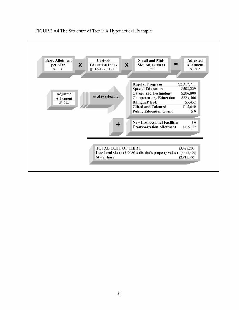
Figure A4 represents the basic 2003-04 Tier I structure for a hypothetical district of 820

students in Refined Average Daily Attendance. This district has a CEI value of 1.05, an

effective tax rate for Maintenance and Operations of $1.32, and a certified property value

of $71,592,881.

31

FIGURE A4 The Structure of Tier I: A Hypothetical Example

Insert Figure 2.3.1.a: Tier I program costs]

TOTAL COST OF TIER I $3,428,205 Less local share ($.0086 x district’s property value) ($615,699) State share $2,812,506

Adjusted Allotment

$3,202 =

Small and Mid-Size Adjustment

1.219 x

Cost-of-Education Index ((1.05-1) x .71) + 1

x Basic Allotment

per ADA $2, 537

Adjusted Allotment

$3,202

used to calculate

Regular Program $2,317,711 Special Education $503,229 Career and Technology $206,800 Compensatory Education $223,566 Bilingual/ ESL $5,452 Gifted and Talented $15,640 Public Education Grant $ 0

New Instructional Facilities $ 0 Transportation Allotment $155,807+

32

The CEI and Tier I

As Figure A4 illustrates, the CEI is the first adjustment to the Basic Allotment. It

increases funding per student to account for differences in resource costs that are beyond

a school district’s control. Each district’s CEI is applied to 71 percent of the Basic

Allotment to calculate the Adjusted Basic Allotment using the following formula:

ABA = 2,537 × (((CEI-1) × .71) + 1)

Depending upon a district’s CEI, the resulting ABA currently ranges from $2,573 to

$2,897 per student in average daily attendance. For many districts, this number is further

adjusted by the Small and Mid-Sized District Adjustment, meaning that overall, the CEI

affects all Tier I adjustments to the Basic Allotment. The CEI does not, however, affect

the calculation of the New Instructional Facilities Allotment or the Transportation

Allotment.

Tier II

Tier II is the “Guaranteed Yield Program.” Tier II guarantees a revenue yield for each

penny of tax effort18 for Maintenance and Operations (M&O) above the 86 cents required

for Tier I.19 Districts may levy M&O taxes at any rate between $.86 and $1.50 per $100

of property valuation. In return, the state guarantees that districts will generate no less

than $27.14 per penny of tax per Weighted Student in WADA from a combination of

state and local resources.

The CEI and Tier II

The CEI interacts with the Guaranteed Yield Program in the way that WADA is

calculated. The WADA figure for each district is based on the sum of the district’s Tier I

allotments (the Basic Allotment, CEI, and Small or Mid-Sized Adjustment, plus funding

for special education, career and technology, gifted and talented, compensatory

education, bilingual/ESL, and Public Education Grant (PEG) programs) less the new

33

instructional facilities allotment, transportation allotment, and 50 percent of the effects of

the CEI.

WADA is used to calculate each district’s Tier II funding (for eligible districts) and the

equalized wealth level under Chapter 41 using the following formula:

GYA = ($27.14 × WADA × DTR × 100) – LR

WADA = number of weighted students in average daily attendance

DTR = the district’s effective Maintenance and Operation (M&O) tax rate over

$.86 per $100 of valuation, not to exceed $.64

LR = the district’s local revenue

A popular misunderstanding about the CEI is that it is simply a mechanism for

increasing state aid to large urban school districts. Every Texas school district has a CEI

value greater than 1.0, however, which means that every school district receives some

adjustment to its Foundation Program calculations to compensate for uncontrollable

variations in the costs of education.

Figure A5 illustrates the effect of the existing CEI on the distribution of net state aid to

Texas school districts, by district size in terms of enrollment. Net state aid is calculated as

state aid to the enrollment group less any amount recaptured from the enrollment group.

In 2002-2003, the fourteen largest districts, which all have enrollments of 50,000 or

greater and which educated more than a quarter of the students in Texas, received

approximately 30 percent of their net state aid as a result of the CEI. Districts with

between 3,000 and 4,999 students in average daily attendance received about 13 percent

of their state aid due to the CEI. It should be noted, however, that the fact that districts

with larger enrollments receive more state aid arises primarily from the fact that the

largest school districts are located in expensive urban areas. Smaller districts in the same

vicinity also have high CEI values. The two districts with the highest existing CEI values

are La Joya ISD (enrollment 19,000) and Roma ISD (enrollment 6,100), both of which

have CEI values of 1.20.

34

Figure A5 The Impact of the CEI on Net State Aid 2003-04

�

$-

$200

$400

$600

$800

$1,000

$1,200

$1,400

$1,600

$1,800

$2,000

UNDER500

500 TO999

1000 TO1599

1600 TO2999

3000 TO4999

5000 TO9999

10000 TO24999

25000 TO49999

50000AND

OVER

Mill

ions

Enrollment Groupings

Additional State Aid Due to CEI

State Aid Without CEI

Figure A6 illustrates another perspective on the effect of the existing CEI on the

distribution of state aid to school districts, in terms of net state aid per student in average

daily attendance. School districts with 50,000 students or more receive, on average and

on net, $376 out of $1,629 in state aid per average daily attendance as a result of the CEI.

School districts with 500 to 999 students receive $213 out of $3,861 in net state aid per

average daily attendance.

35

Figure A6 Impact of Existing CEI on Net State Aid per ADA 2003-04

-

500.00

1,000.00

1,500.00

2,000.00

2,500.00

3,000.00

3,500.00

4,000.00

4,500.00

UNDER500

500 TO999

1000 TO1599

1600 TO2999

3000 TO4999

5000 TO9999

10000 TO24999

25000 TO49999

50000AND

OVER

Enrollment Groupings

State Aid per ADA Due to CEIState Aid per ADA Without CEI

Notes

17 Multiple regression is a mathematical model that takes account of the effect of more than one independent factor or variable on a dependent variable. In the case of the 1991 CEI, the dependent variable was the natural logarithm of teacher salaries. 18 “Tax effort” is not the same as “tax rate.” A district’s tax effort is calculated on the basis of its tax collections divided by the Comptroller’s certified taxable property values. 19 Districts can also levy taxes to pay existing debt (Interest and Sinking, or I&S taxes), but the state provides a different level of support for a district’s I&S tax effort.

Appendix B: Data Revisions

The data differ from those in the 2000 and 2001 Dana Center reports in a number

of important ways. Changes in labor market definitions have moved 71 school districts

from the rural category to the urban category and 17 districts from the urban category to

the rural category. (Micropolitan statistical areas are considered rural in this analysis.)

The addition of new counties to the metropolitan areas, the consolidation of some MSAs,

and the combination of some counties into micropolitan areas has altered our measures of

average house price, average cooling-degree days, population density, and distance to the

center of the nearest metropolitan area. The new labor -market definitions also allow us

to include an indicator for whether or not the district is located in a micropolitan area.

The Bureau of Labor Statistics has revised its estimates of unemployment rates (although

it has not yet incorporated the new market definitions) and we have more data from

which to calculate the trend rate of unemployment. (Our indicator is deviation from

trend.) We have introduced a new variable for time in field of certification and have

combined the previous indicators of traditionally and nontraditionally certified into a

single indicator for whether or not the individual holds any type of teaching certificate.

We have modified the treatment of school district size. The Dana Center report

estimated the relationship between compensation and the log of average daily attendance

(ADA), its square and an indicator for ADA > 80,000. However, when scoring the index,

they followed the convention of the existing CEI and assigned an ADA of 15,000 to all

districts with ADA above 15,000. In effect, both the Dana Center report and the existing

CEI treat any costs associated with having an ADA > 15,000 as controllable costs.

Rather than make such an assumption, we constructed an alternative measure of school

district size and used it both to estimate the models and to score the index. Our measure

takes on the value of log(ADA) for all districts with ADA < 25,000 and takes on the

value of log(25,000) for all other districts. For urban districts, we also include the square

of our ADA measure and indicator variables for ADA between 25,000 and 50,000 and for

ADA greater than 50,000 (the two largest TEA size categories). We note that there are

no rural districts with ADA > 15,000 so these changes are not relevant for the rural

estimation.

37

We have revised data on school location. Where the Dana Center analysts used

campus zip codes to assign latitude and longitude to Texas schools, we now have latitude

and longitude information from the National Center for Education Statistics’ Common

Core of Data (CCD). The CCD contains latitude and longitude data on two-thirds of

Texas campuses. The remaining campuses continue to be assigned latitudes and

longitudes according to the zip codes at their street address. Comparing the latitude and

longitude assigned by CCD to those implied by zip codes indicates that the average

difference between the two locational indicators is less than 3 miles, but it can reach 25

miles in some parts of the state.

We have revised data on population density. The current analysis uses data from

the 2000 Census to identify teacher markets that are densely populated, sparsely

populated, and very sparsely populated.

We have revised the data on teacher experience. With additional years of

information, we were able to construct much longer experience profiles for each Texas

teacher. Those profiles allowed us to impute plausible experience values for some of the

individuals who were omitted from the original analysis because their stated level of

experience was implausible. The more complete profiles also allowed us to identify

individuals with implausible experience values who should have been omitted from the

original analysis but were not because their experience level could not be identified as

anomalous.

Finally, for purposes of analysis and to construct the index values, we rely on

three-year moving averages of the uncontrollable cost factors. Thus, the estimation and

indexing for 1999 reflects the average school district characteristics for 1997, 1998, and

1999. Smoothing the data in this way removes anomalous year-to-year variation in the

data and makes the index values more consistent from one year to the next.