Pattern-Based Predictive Control for ETBE

Reactive Distillation

Yu-Chu Tian 1, Futao Zhao, B. H. Bisowarno, Moses O. Tade

Department of Chemical Engineering, Curtin University of Technology, GPO BoxU1987, Perth WA 6845, Australia

Abstract

Synthesis of ethyl tert-buty ether (ETBE), a high-performance fuel additive, throughreactive distillation (RD) is an attractive route, while its operation and controlare exceptionally difficult due to its functional combination and complex dynamics.Modern control technology greatly relies on good process models, while a reasonableRD model is too complex for control design. Moreover, RD contains considerableuncertainties that cannot be well described in process modelling. Alleviating themodel requirement, this work aims to maintain the product purity in RD of ETBEthrough developing a pattern-based predictive control (PPC) scheme. Process dy-namics, control structure, nonlinear transformation, feature pattern extraction, andpattern-based prediction and its incorporation with a conventional linear controllerare discussed. Case studies show the effectiveness of the proposed method.

Key words: reactive distillation, time delay, predictive control, feature patterns,fuzzy logic

1 Introduction

Reactive distillation (RD), a simultaneous implementation of sequential reac-tion and distillation in a countercurrent column, is an old idea; however, ithas received renewed attention in the recent years and is becoming increas-ingly important in industry [1,2]. It has demonstrated potential improvementsin capital productivity and selectivity, and reduction in solvents, energy con-sumption, and capital investments. Some improvements are dramatic, as de-scribed in [2] for a methyl acetate RD process: 5 times lower investment and

1 Author to whom all correspondence should be addressed. Phone: +61 8 9266 3776,fax: +61 8 9266 2681. E-mail: tiany@che.curtin.edu.au (Y.-C. Tian).

Preprint submitted to Elsevier Preprint 18 December 2001

5 times lower in energy consumption by using a hybrid RD process to re-place an entire flowsheet with 11 units and related heat exchangers, pumps,intermediate storage vessels, and control systems!

RD is advantageous for a great number of chemical syntheses, including fuelether production, which is the focus of this work. As fuel additives, fuel ethershave been widely used for improvement of fuel quality. In a continuous effortfor development and production of high-performance fuel additives, RD hasbeen successfully applied in the synthesis of the widely used methyl tert-butylether (MTBE), which has a dual advantage in fuel lead removal and oxygenateintroduction.

Current research has focused on MTBE, while recent studies reveal thatMTBE has severe water ingress problem that may pollute underground water.Ethyl tert-butyl ether (ETBE) has been found to be a potential alternative toMTBE due to its higher performance, less water contamination, and synthesisfrom semi-renewable products (ethanol from biomass).

RD has been found to be feasible for ETBE production, while the RD ofETBE is still limited worldwide and needs to be commercialised. Moreover,RD involves considerable uncertainties and displays complex behaviour suchas high non-linearity, strong interactions, bifurcation and multiplicity, andtime delay. RD dynamics and behaviour are yet to be fully understood. Dueto the functional integration of reaction and separation, and the dynamicscomplexity, RD is exceptionally difficult to operate and control. This calls forsystematic research on RD process dynamics and control aspects.

The work is done on a pilot-scale RD column for ETBE production at ourlaboratory. In RD of ETBE, reactant conversion and product (ETBE) purityare two key process variables. The former is a measure of the usage of the rawmaterials, while the latter characterises the product quality. Both of them aredirectly related to the productivity of the process. This work will address themaintenance of the purity of product (ETBE), which is withdrawn from thebottom of the RD column.

The ETBE purity will be controlled indirectly by regulating a column tem-perature. Because the desired purity (purity set-point) may be changed inplant operation, the control system should have a fast set-point tracking abil-ity (tracking problem). On the other hand, RD and other chemical processesalways have various disturbances and uncertainties, which cannot be well mod-elled and predicted, resulting in a requirement of effective disturbance rejec-tion (regulatory problem). Control design should consider both tracking andregulatory problems for RD processes.

A good process model is the basis of modern control technology. Althoughit is possible to develop a reasonable model for specific RD processes [3,4],

2

such a model is too complex for control design. Furthermore, RD processescontain a large degree of uncertainties that cannot be well described in processmodelling.

To alleviate the model requirement, this work develops a pattern-based pre-dictive control (PPC) scheme incorporating with conventional proportional-integral (PI) controller for the non-linear and complex RD process. Similarideas have been used for processes with time delay [5]. The process dynam-ics, control structure, non-linear transformation, and pattern extraction andutilisation for process prediction will be discussed in detail. Case studies willshow the effectiveness of the proposed approach.

2 Process Description

The chemical structure of ETBE is (CH3)2COC2H5. It is produced fromethanol and a mixed C4 olefine stream containing isobutylene (typically ofa cracking unit product). The dominant chemical reaction in ETBE synthesisis the reversible reaction of isobutylene and ethanol over an acid catalyst toform ETBE

(CH3)2C = CH2 + C2H5OH ⇐⇒ (CH3)3COC2H5 (1)

The acidic ion-exchange resin, Amberlyst 15, is used in our work. The reactionis equilibrium limited in a range of temperatures. The reaction kinetics hasbeen investigated in [6] and discussed in [3], from where detailed expressionsfor the equilibrium constant and rate equation are available.

Two side reactions exist in ETBE synthesis. One is the dimerisation of isobuty-lene to form diisobutylene (DIB) with the chemical structure of [(CH3)2C=CH2]2.In the presence of any water in the reaction environment, another side reactionis the hydration of isobutylene to form isobutanol (isobutyle alcohol) with thechemical structure of (CH3)3COH. The side reactions are expressed by

(CH3)2C = CH2 + (CH3)2C = CH2⇐⇒ [(CH3)2C = CH2]2 (2)

(CH3)2C = CH2 + H2O⇐⇒ (CH3)3COH (3)

A pilot-scale RD column has been built at our laboratory for ETBE (andMTBE) production. It is graphically shown in Figure 1. With a diameterof 0.155m and a height of 4.1m, the column consists of three sections forrectifying, reaction, and stripping, respectively, and is filled with two novelpackings, one of which contains the catalyst, Amberlyst 15, which is necessary

3

for the etherification reaction. The RD process has a total condenser and apartial reboiler.

The column is estimated to have 8 theoretic stages: 1, 3, and 4 stages in recti-fying, reactive, and striping sections, respectively. The condenser and reboilerare considered as two separate stages. Therefore, there are 10 stages alto-gether, which are numbered from top to bottom as shown in Figure 1. Therectifying section has only one stage (stage 2); the reactive section has 3 stages(stages 3, 4, and 5); and the stripping section has 4 stages (stages 6 to 9). Theraw material is fed at stage 6; while the final product, ETBE, is withdrawnfrom stage 10 (reboiler). Measurement points are also indicated in Figure 1 fortemperature, flow rate, pressure, and level variables. More information aboutthe the architecture of the RD process can be found in [3,4,7].

A typical set of operating conditions of the RD process for ETBE synthesis istabulated in Table 1. It will be considered as the nominal situation, at whichthe control system for the ETBE purity will be designed.

3 Control System Configuration

RD control is challenging due to high non-linearity, strong interactions, bi-furcation and multiplicity, time delay, process uncertainties, and the largenumber of possible control configurations. From the control point of view, anRD process has 5 degrees of freedom for control design, i.e. 5 process variablescan be manipulated (control inputs): flow rates of reflux(L), boil-up (V ), dis-tillate (D), bottoms (B), and column top vapour VT . The reflux ratio L/Dcan be used instead of L for control design. In our pilot-scale RD process, theflow rates of boil-up (V ) and column top vapour (VT ) are characterised byreboiler duty (Qr) and condenser duty (Qc). The controlled variables (con-trol objectives) are reflux accumulator and reboiler levels, column pressure,bottoms (ETBE) purity, and reactant conversion. Typical disturbances to theRD process include changes in feed composition (Fc), which is characterisedby the stoichiometric ratio, and in feed flow rate (Ff ).

In practice, three control loops are designed for inventory and pressure con-trol. The control configuration problem addressing which of the five degreesof freedom should be used in those three loops has been extensively discussed,e.g. [8]. Two more loops can be designed for purity and conversion control.The resulting control configuration is conventionally named by the two in-dependent variables that are used for composition (purity) control, e.g. LV,LB, D/V, (L/D)(V/B), etc. Among all possible control structures includingratio schemes and those with consideration of feed flow rate Ff , non-ratioschemes LV and LB has been shown to be preferred for the RD column under

4

consideration [4]. This work will consider the LV configuration.

In the LV configuration of the RD process, the column pressure is maintainedby manipulating the condenser duty Qc; the inventory control for reflux accu-mulator and reboiler hold-up is implemented by adjusting the distillate flowrate D and bottoms flow rate B, respectively. The reflux flow rate L is fixedwhile the reboiler duty Qr is manipulated for product (ETBE) purity. This isa typical one-point control problem in RD processes.

The purity control is important, while it is not easy because the purity char-acterised by composition is difficult to measure in real time reliably and eco-nomically. Fast and reliable measurement of the controlled variable is a basicrequirement of closed-loop control.

A method to overcome this difficulty is to implement inferential control forthe purity. In this method, an inferential model has to be developed to inferthe purity from multiple measurements that are easily obtained, e.g. multiplecolumn temperatures. Progress has been made in this direction [9,7].

An alternative method to overcome the difficulty is to indirectly control thepurity by controlling some other process variables that are easy to obtain andare indicators of the purity. However, such indicators are not easy to find dueto the unavailability of a one-to-one relationship between a single variable andthe purity. In distillation column control practice, column temperatures areusually used for indirect composition control.

The reboiler temperature reflects the dynamic changes of the ETBE purityquickly, while it is not a good purity indicator since a single reboiler tem-perature value may correspond to multiple purity values [7]. In this work,the stage 7 temperature T7 is used for inference and control of the product(ETBE) purity for the RD process under consideration.

4 Process Dynamics

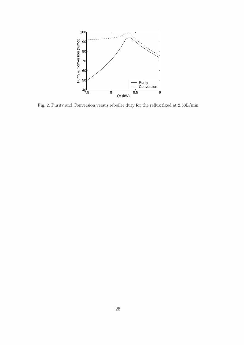
The steady state relationship between the ETBE purity and the reboiler dutyQr for a fixed reflux flow rate is shown in Figure 2 [7]. Qr = 8.45kW is aroundan optimal Qr value that gives the maximum value of the ETBE purity. It ischosen as the nominal operating point.

The steady state relationships between T7 and Qr are investigated under dif-ferent reflux flow rates and are graphically depicted in Figure 3. It is clearlyseen from Figure 3 that there exists a significant non-linearity in process gainkp (kp is high within an operating range of Qr but becomes small outside this

5

range), and the reflux flow rate L affects the T7 versus Qr relationship in acomplex manner.

The ETBE purity versus Stage 7 temperature T7 can be easily obtained fromFigures 2 and 3. Although the relationship between T7 and the ETBE purityis non-linear, T7 determines the purity uniquely. Another advantage of usingT7 is that the sensitivity of T7 to the purity is high [4].

It has been found that the RD process has changeable inertia as operatingconditions change, suggesting time-varying process response speed. By con-vention, the inertia is characterised by a time constant or multiple time con-stants.

Detailed investigation also reveals considerable time delay from Qr to T7, im-plying that any manipulation in Qr will not affect T7 until the time delayelapses. The significance of the RD time delay is shown in Table 2. The ex-istence of time delay imposes severe constraints on the control system andcomplicates the control system design.

With a fixed heat input to the reboiler, an increase in feed flow rate Ff willresult in an increase in bottoms flow rate and consequently a decrease in thetemperatures below column stage 6. On the other hand, the feed stoichiometricratio characterising the feed composition has a positive effect on T7, i.e. anincrease in the ratio will lead to an increase in T7. Changes in feed flow rate Ff

and feed composition Fc are primary disturbances to the process operation.These disturbances affect T7 dynamics significantly in a complex manner, e.g.nonlinear gain, time-varying inertia, and time delay, which are similar to butdifferent in value from those from Qr to T7.

Simplified input-output process models expressed by transfer functions for ma-nipulation and disturbances are identified under specific operating conditions.The identified results are first-order plus time delay descriptions, which aretabulated in Table 2. Table 2 shows the RD process dynamics quantitatively.For example, the process gain, time constant, and time delay all change ina wide range as process operating conditions change. While more complexexpressions of T7 dynamics can be precisely established from the first princi-ples of mass balance and energy balance, e.g. [3,4], these types of models aredifficult to use for control design.

5 Pattern-Based Predictive Control

Due to the complexity of the RD process dynamics, conventional controltechnologies, e.g. PI control, cannot provide satisfactory control performance,

6

while the application of modern control technology requires good process mod-els. A reasonable process model as described in [3,4] contains hundreds ofequations for the 10-stage RD process under consideration. It is too compli-cated to be directly used for control system design. Simplified input-outputprocess models discussed in the last section are helpful in understanding thecomplex process dynamics, but they are identified under some specific op-erating conditions and thus cannot represent the process in a wide range ofoperating conditions. Although it is possible to extend the transfer functionmodels, again this will complicate the control system design. Furthermore,the RD process contains a large degree of uncertainties, which cannot be welldescribed using any type of mathematical expressions. Therefore, techniqueswithout using exact process models are more attractive for RD control.

Pattern-based predictive control (PPC) is such a method that does not rely onexact process models while providing improved control performance for com-plex processes over conventional, e.g. PI, control algorithms. Some progresshas been made in this direction, e.g. for time delay compensation [5], adaptivePI [10], fuzzy predictive control [11], etc.

The proposed PPC system for the RD process is schematically depicted inFigure 4, which is a further development of the authors’ previous work [5]that considers linear processes. It consists of two main parts: a non-lineartransformation u = f(v) and a pattern-based predictor (PP). The formeris used for input-output linearisation of the process gain, while the latter isemployed to anticipate process output some (e.g. d) steps ahead. The PPutilises process feature patterns qualitatively and quantitatively, which areextracted from the controlled and manipulated variables, and is incorporatedwith a conventional controller Gc (e.g. PI) in the PPC system. For the RDsystem, y and u in Figure 4 correspond to T7 and Qr, respectively.

Ideally, The PP acts as a time lead component as it provides d steps aheadprediction of the controlled variable. It will effectively compensate for thetime delay in the the RD process and thus allows more aggressive controllersettings compared with the control systems without PP. Therefore, the PPCwill provide improved performance in both set-point tracking and disturbancerejection, as will be shown later for the RD process.

The nonlinear transformation, feature pattern extraction, and PP design willbe respectively discussed in the successive sections.

7

6 Nonlinear Transformation

Because the process has a highly nonlinear process gain, which will degradethe prediction performance of the PP, a nonlinear transformation

u = f(v) (4)

is introduced to obtain a v ∼ y relationship with a pseudo linear gain, wherev is the new manipulated variable. This is a type of input-output linearisation[12], which is one of the most widely used techniques for nonlinear controlsystem design.

Notice that controlling a process always requires a certain degree of under-standing of the process. The rough knowledge of the process gain can beobtained a priori, which is sufficient to construct such a nonlinear transfor-mation. Moreover, a linear PP can accommodate a certain degree of processuncertainties, implying that no exact nonlinear transformation is required.

The process gain kp can be determined by the derivatives of the curves inFigure 3. Let g(u) denote the steady state input-output relationship of Figure3, i.e.

y = g(u) (5)

Ideally, f(v) is designed such that y is linear to the new manipulated variablev, i.e.

y = g[f(v)] = bv + c (6)

where b is a constant representing the gain of the input-output linearisedsystem; c is also a constant representing the bias. It follows that f(v) is theinverse of g(bv + c), i.e.

f(v) = g−1(bv + c) (7)

The determination of the constants b and c is straightforward and can be doneat the operating point of the RD process. Tables 1 and 2 shows that at theoperating point, Qr = 8.45kW, T7 = 133.12◦C, kp = 49.28◦C/kW. Supposethat these values are retained in the input-output linearised system. Accordingto equation (6 ), we have

b = 49.28, c = −283.2960 (8)

8

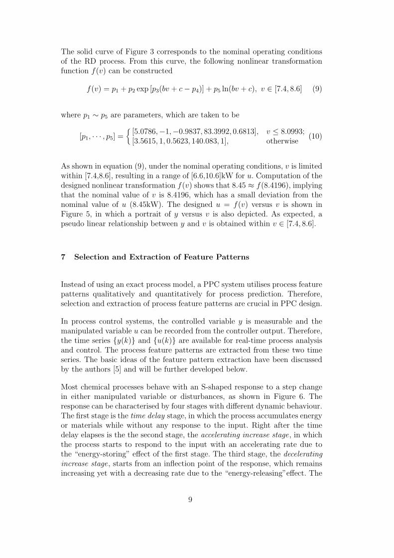
The solid curve of Figure 3 corresponds to the nominal operating conditionsof the RD process. From this curve, the following nonlinear transformationfunction f(v) can be constructed

f(v) = p1 + p2 exp [p3(bv + c− p4)] + p5 ln(bv + c), v ∈ [7.4, 8.6] (9)

where p1 ∼ p5 are parameters, which are taken to be

[p1, · · · , p5] ={

[5.0786,−1,−0.9837, 83.3992, 0.6813], v ≤ 8.0993;[3.5615, 1, 0.5623, 140.083, 1], otherwise

(10)

As shown in equation (9), under the nominal operating conditions, v is limitedwithin [7.4,8.6], resulting in a range of [6.6,10.6]kW for u. Computation of thedesigned nonlinear transformation f(v) shows that 8.45 ≈ f(8.4196), implyingthat the nominal value of v is 8.4196, which has a small deviation from thenominal value of u (8.45kW). The designed u = f(v) versus v is shown inFigure 5, in which a portrait of y versus v is also depicted. As expected, apseudo linear relationship between y and v is obtained within v ∈ [7.4, 8.6].

7 Selection and Extraction of Feature Patterns

Instead of using an exact process model, a PPC system utilises process featurepatterns qualitatively and quantitatively for process prediction. Therefore,selection and extraction of process feature patterns are crucial in PPC design.

In process control systems, the controlled variable y is measurable and themanipulated variable u can be recorded from the controller output. Therefore,the time series {y(k)} and {u(k)} are available for real-time process analysisand control. The process feature patterns are extracted from these two timeseries. The basic ideas of the feature pattern extraction have been discussedby the authors [5] and will be further developed below.

Most chemical processes behave with an S-shaped response to a step changein either manipulated variable or disturbances, as shown in Figure 6. Theresponse can be characterised by four stages with different dynamic behaviour.The first stage is the time delay stage, in which the process accumulates energyor materials while without any response to the input. Right after the timedelay elapses is the the second stage, the accelerating increase stage, in whichthe process starts to respond to the input with an accelerating rate due tothe “energy-storing” effect of the first stage. The third stage, the deceleratingincrease stage, starts from an inflection point of the response, which remainsincreasing yet with a decreasing rate due to the “energy-releasing”effect. The

9

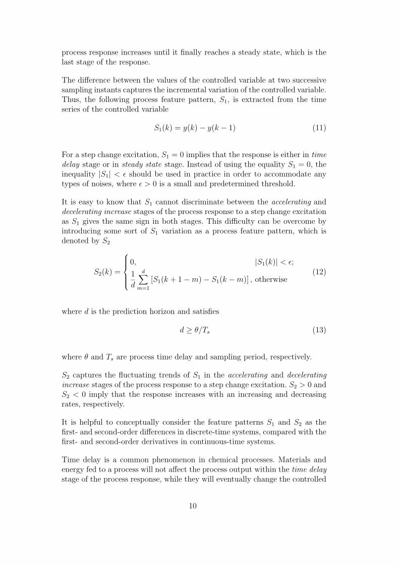
process response increases until it finally reaches a steady state, which is thelast stage of the response.

The difference between the values of the controlled variable at two successivesampling instants captures the incremental variation of the controlled variable.Thus, the following process feature pattern, S1, is extracted from the timeseries of the controlled variable

S1(k) = y(k)− y(k − 1) (11)

For a step change excitation, S1 = 0 implies that the response is either in timedelay stage or in steady state stage. Instead of using the equality S1 = 0, theinequality |S1| < ε should be used in practice in order to accommodate anytypes of noises, where ε > 0 is a small and predetermined threshold.

It is easy to know that S1 cannot discriminate between the accelerating anddecelerating increase stages of the process response to a step change excitationas S1 gives the same sign in both stages. This difficulty can be overcome byintroducing some sort of S1 variation as a process feature pattern, which isdenoted by S2

S2(k) =

0, |S1(k)| < ε;

1

d

d∑

m=1

[S1(k + 1−m)− S1(k −m)] , otherwise(12)

where d is the prediction horizon and satisfies

d ≥ θ/Ts (13)

where θ and Ts are process time delay and sampling period, respectively.

S2 captures the fluctuating trends of S1 in the accelerating and deceleratingincrease stages of the process response to a step change excitation. S2 > 0 andS2 < 0 imply that the response increases with an increasing and decreasingrates, respectively.

It is helpful to conceptually consider the feature patterns S1 and S2 as thefirst- and second-order differences in discrete-time systems, compared with thefirst- and second-order derivatives in continuous-time systems.

Time delay is a common phenomenon in chemical processes. Materials andenergy fed to a process will not affect the process output within the time delaystage of the process response, while they will eventually change the controlled

10

variable in the later stages. Therefore, the time series of the manipulatedvariable also contain information of the future process output.

Instead of the real manipulated variable u, the transformed manipulated vari-able v will be used in feature pattern extraction. The magnitude of v is alreadyreflected in the feature patterns S1 and S2, while the incremental variation ofv characterising additional excitation has not been covered by either S1 orS2. The following feature pattern S3 captures the incremental variation of vduring the time period [k − d, k]

S3 =d∑

m=1

[v(k + 1−m)− v(k − d)] (14)

In geometry, S3 reflects the area bounded by the curve v(k) and the straightline crossing the point (k − d, v(k − d)) over the time period [k − d, k]. Itinfluences the process output in a complex manner, which needs more fea-ture patterns to characterise. The following feature pattern S4 can assist indetermining the effect of S3 on the process output.

S4 =

0, |S3(k)| < ε;∣∣∣∣∣1

S3

d∑

m=1

m[v(k + 1−m)− v(k − d)]

∣∣∣∣∣ , otherwise(15)

8 Pattern-Based Fuzzy Prediction

The d steps ahead prediction of the controlled variable is carried out using thefollowing simple formulae, which are based on the extracted process featurepatterns

y(k + d|k) = y(k) + ∆y(k + d|k) (16)

∆y(k + d|k) = r1 [S1(k) + r2S2(k)] + r3(k)S3(k) + h(k)∆y(k|k−d) (17)

where r1 ∼ r3 are three coefficients; h > 0 is an updating factor for real-timeadaptation.

h can be simply chosen to be a constant, implying that a fixed step is used.The following variable step algorithm is employed in this work for updating h

h(k) = h(k − 1) + ∆h(k) (18)

where ∆h(k) is designed to be 0 if |∆y(k|k−d)| < 0.001, and 0.01|∆y(k|k−d)|

11

if |∆y(k|k−d)| > 0.1 and |∆y(k|k−d)−∆y(k − 1|k−d−1)| < 0.001. For all otherconditions, take ∆h(k) = 0.01sign [∆y(k|k−d)−∆y(k − 1|k−d−1)] ∆y(k|k−d).

The determination of the values of the parameters r1 and r2 relies on anestimate of the ratio T/θ. However, r1 and r2 are fixed for a specific value ofT/θ. They should be proportional to the prediction horizon d and should bea function of the ratio T/θ. The following heuristic relations can be used todetermine r1 and r2

r1/d = 0.6622 + 0.0244(T/θ)− 0.5482 exp (−2.1T/θ) (19)

r2/d = 0.2039 + 0.0047(T/θ)− 0.1797 exp (−2T/θ) (20)

Equation (20) has extended the guideline for r2 determination in a table formin [5], where the parameter r2 was integrated into the feature pattern S2.

A compact, explicit, and satisfactory expression for r3 has not been establisheddue to the complex influences of the feature patterns S3 and S4 on the processoutput. However, our experience tells us that r3 should be determined basedon the ratio T/θ and the feature pattern S4. Therefore, a set of fuzzy logicrules is developed to describe r3 qualitatively and quantitatively.

Let FSx denote the fuzzy set of the variable x ∈ {T/θ, S4, r3}. Each of thethree fuzzy sets uses three linguistic terms: big (B), medium (M), and small(S), to represent, in an approximate and quantised way, the magnitude ofthe corresponding variable. Let Ai

x ∈ {B, M, S} denote a specific linguisticvalue of FSx in the ith fuzzy rule, x ∈ {T/θ, S4, r3}. The triangle membershipfunction, denoted by µ(·) → [0, 1], is used for the fuzzy sets FST/θ and FSS4 ,as shown in Figure 7.

Corresponding to Air3∈ {B, M, S}, three central numerical values denoted

by V (Air3

) can be identified using, say, the least-squares technique. The fuzzylogic rules take the If-Then form, e.g.

Ri: If(T/θ is Ai

T/θ

)and

(S4 is Ai

S4

)Then r3 is V

(Ai

r3

)(21)

Combining FST/θ and FSS4 , 5 fuzzy rules are designed, which are tabulated inTable 3. These rules are schematically depicted in Figure 7. The computationof the degrees of fulfillment for these rules is also shown in Table 3 [13]

Finally, the parameter r3 is computed over the entire fuzzy rules using thefollowing defuzzification formula

r3(k) =5∑

i=1

[βiV

(Ai

r3

)]/

5∑

i=1

βi (22)

12

It is worth mentioning that for a specific application, if T/θ is not time-varying,the number of rules, and thus the number of βi in Table 3, will be reduced to3, as will be discussed in the case studies in the next section.

9 Case Studies

9.1 System Configuration

The developed pattern-based predictive control (PPC) strategies are used forpurity maintenance in RD of ETBE. The purity is controlled indirectly by con-trolling the stage 7 temperature T7 of the RD column; while T7 is maintainedby manipulating the reboiler duty Qr. This is a one-point control problem inRD.

For the RD process under consideration, as shown in Table 2, T = 15.6minand θ = 7min under the nominal operating conditions. Ts and ε are set to be1min and 10−5, respectively. According to equation (13), set d = 8. The initialvalue of h is taken to be 0.1.

For process prediction using equation (17), r1, r2, and r3 are required. Equa-tions (19) and (20) give r1 = 5.6919 and r2 = 1.6983. r3 is obtained throughfuzzy logic inference.

For the specific RD control problem, T/θ = 15.6/7 is already known, whichis Big with µ (T/θ is B) = 1 as shown in Figure 7. Therefore, the rules R3

and R5 in Table 3 are excluded and the remaining rules R1, R2, and R4 aresimplified to

R1: If (S4 is B) Then r3 is V (S)

R2: If (S4 is M ) Then r3 is V (M)

R4: If (S4 is S ) Then r3 is V (B)

(23)

which correspond to the first row of Figure 7. Consequently, β1, β2, and β4 inTable 3 are reduced to

β1 = µ(S4 is S), β2 = µ(S4 is M), β4 = µ(S4 is S) (24)

Taking into account Figure 7, the computation of equation (24) is shown inTable 4.

13

It is seen from Table 4 that β1 + β2 + β4 = 1 for any specific values of S4,implying that equation (22) for r3 computation is reduced to

r3 = β1V (S) + β2V (M) + β4V (B) (25)

As also shown in Table 4, the relationship in equation (25) can be furthersimplified for specific values of S4 due to the fact that one or more βi = 0.Three values of V (B), V (M), and V (S) have been identified to be 2.4510,1.0622, and −1.9974, respectively.

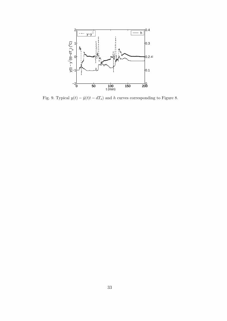
Typical curves of v(t), y(t), y(t|t − dTs), y(t) − y(t|t − dTs), h(t), and S1 toS4 are shown in Figures 8, 9, and 10. It is seen from these figures that the dsteps ahead prediction of y matches the real y very well, and the predictionerror is within ±1.5◦C (±1.25% of the real y) for the v with gradual andsharp changes. h is updated if prediction error exists, as shown in Figure9. However, in this example, h (< 0.21) contributes at most 0.26◦C to theprediction, implying that the adaptive term, i.e. the last term of equation (17),weighs about 0.26/133 ≈ 0.2% of the total predicted quantity and is actuallynegligible. Thus, the prediction is mainly based on the feature patterns S1 toS4 shown in Figure 10.

The PP is incorporated with a conventional PI controller, which is tuned forset-point tracking for the index of the integral of time-weighted absolute error(ITAE). The controller settings are kc = 0.1331 and Ti = 22.1min. Thosesettings can ensure the control performance and stability in a wide range ofoperating conditions.

The performance of the PPC is evaluated and compared with that of a directPI control for the RD column. Both setpoint tracking and disturbance rejectionresponses will be considered. The direct PI controller is also tuned in the rangeof operating conditions for set-point tracking for the ITAE index, resulting inmore conservative settings kc = 0.0203 and Ti = 19.9min, compared with thePI controller settings in the PPC system.

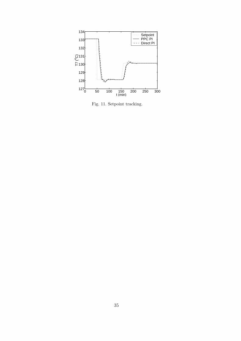
9.2 Set-Point Tracking

For set-point tracking, a −5◦C step change and a +2◦C ramp change in T7

setpoint are introduced at time instants 50min and 150min, respectively. Thecontrol results are given in Figure 11, which shows that less overshoot andshorter settling time are obtained from the PPC system. The PPC systemimproves the ITAE index by over 25% over the direct PI control system, asshown in Table 5.

14

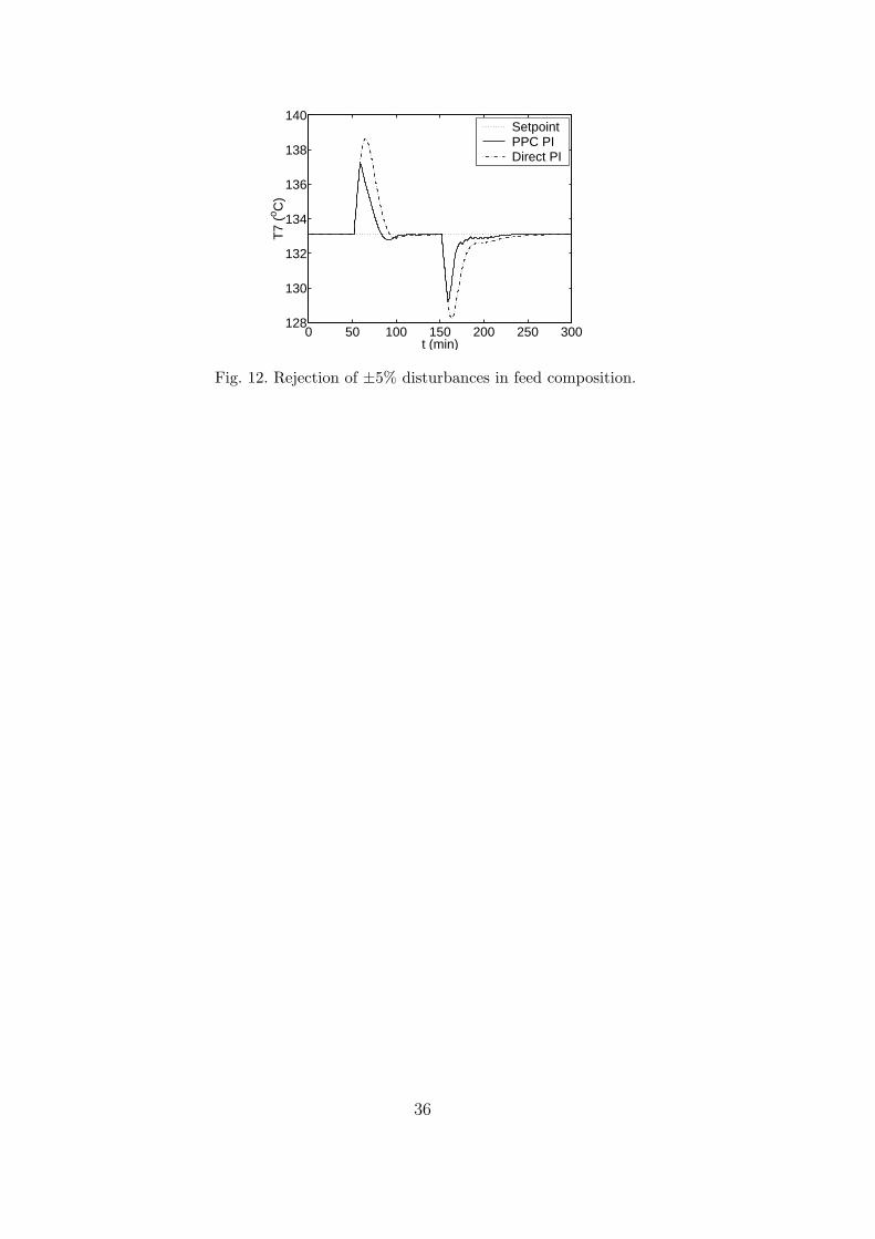
9.3 Rejection of Feed Composition Disturbances

Changes in feed composition, which is represented by the stoichiometric ratio,are disturbances to the RD column. ±5% (i.e. ±0.25) step changes in feed com-position are introduced to the process in order to test the disturbance rejectionability of the PPC system. The step changes occur at the time instants 50 and150min, respectively. Figure 12 depicts the control results, which show thatPPC provides significant improvement over the disturbance rejection ability.The ITAE index improvement reaches over 50%, as shown in Table 5.

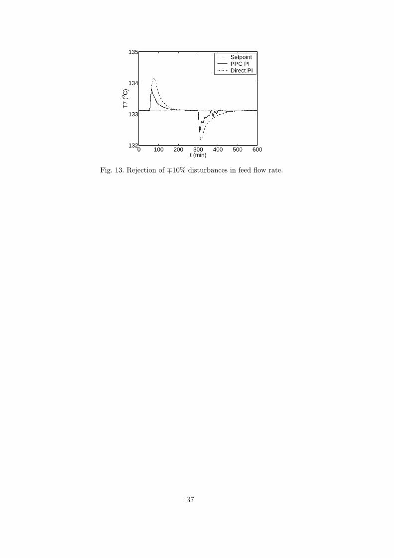
9.4 Rejection of Feed Rate Disturbances

Changes in feed flow rate are also disturbances to the RD column. ∓10%(i.e. ±0.074L/min) step changes in feed flow rate are introduced at the timeinstants 50 and 300min, respectively. The control results are illustrated inFigure 13, which shows that disturbances in feed flow rate have severe effecton the RD process. The PPC system outperforms the direct PI control systemas it rejects the disturbances much more effectively with much smaller ITAEindices (the improvement > 55%), as shown in Figure 13 and Table 5. Somesort of ratio control involving the feed flow rate is an option for conventionalPI control to improve the disturbance rejection performance, while previousstudies have provided no incentive to configure a ratio control system in thestudied RD column [4].

9.5 Remarks

It is worth mentioning that the RD process is severely nonlinear. Therefore,system analysis and performance evaluation have to be made at the specificoperating point. The nominal RD operating condition for this work is clearlylisted in Table 1. Since this work addresses one-point control (purity controlof the bottoms product), the reflux flow rate has been fixed at 2.53L/min.As a result, the degree of process nonlinearity is reduced. This is why theperformance of the direct PI control is also acceptable in the case studies,although the PPC system does provide improvement over the direct PI control.

Through manipulating the reboiler duty Qr, the stage 7 temperature T7 iscontrolled as the indicator of the bottoms product purity. As shown in Table1 , the nominal value of the purity is 90mol%. The relationship between thepurity and T7 can be easily obtained from Figures 2 and 3.

15

10 Conclusions

RD of ETBE is a non-conventional and complex process with high nonlinearity,strong interactions, bifurcation and multiplicity, time delay, and large degreeof process uncertainties. A PPC system has been developed for the purityof a pilot-scale RD process for ETBE synthesis. Alleviating the requirementof good process models, which are essential for modern model-based control,it utilises feature pattern-based prediction incorporated with conventional PIcontrol. To obtain a pseudo input-output linear process gain, a nonlinear trans-formation is designed, which needs only a rough and easily obtained knowledgeof the steady state characteristics of the process. Four types of process featurepatterns are extracted from the time series of the controlled variable and thetransformed manipulated variable. Fuzzy logic rules driven by the extractedfeature patterns are then developed for process prediction. Case studies haveshown that the PPC can provide improved control performance for both set-point tracking and disturbance rejection. The PPC is a promising tool forcomplex processes, where good process models are difficult to obtain or toimplement for real-time control.

Acknowledgements

The authors would like to thank Australian Research Council (ARC) for itssupport under large and small grant schemes (ARCLGS and ARCSGS). Thefirst author (YCT) also acknowledges the supports from Western Australiastate government under strategic research fellowships, and Curtin Universityof Technology under research grant schemes (CUTRGS) and small discoverygrants schemes.

Nomenclature

Aix ∈ {B, M, S}: a linguistic value of FSx for the ith rule, x ∈ {T/θ, S4, r3}

βi Degree of fullfillment for the ith ruleB Bottoms flow rate (L/min), or the linguistic term “Big”b, c Constants in the nonlinear transformation∆y d steps ahead prediction of the y deviationD Distillate flow rate (L/min)d Number of prediction stepsε Small and positive threshold in S2

f Nonlinear transformation within the PPC systemFc Feed composition (stoichiometric ratio)

16

Ff Feed flow rate (L/min)FSx Fuzzy set of the subscript variable x ∈ {T/θ, S4, r3}g Intermidiate function, at steady state y = g(u)Gc ControllerGL Process transfer function in disturbance pathGp Process transfer function in manipulation pathh Updating factor for process predictionk Present sampling instantkc controller gainkp Process gain (◦C/kW)L Reflux flow rate (L/min) or LoadM The linguistic term “Medium”µ Membership functionp1 ∼ p5 Parameters for nonlinear transformation fQc, Qr Condenser duty and reboiler duty (kW)R Setpointr1 ∼ r3 Parameters for prediction of the controlled variableS The linguistic term “Small”S1 ∼ S4 Process feature patternsT Process time constantT7 Stage 7 temperature (◦C)Ti Controller integral time (min)θ Process time delay (min)Ts Sampling period (min)u Manipulated variable (e.g. reboiler duty)V Boilup flow rate (L/min)v Transformed manipulated variable within the PPC systemV

(Ai

r3

)Central numerical values of Ai

r3∈ {B,M, S}

VT Column top vapour flow rate (L/min)y Controlled variable (e.g. stage 7 temperature)y d steps ahead prediction of y

References

[1] M.F. Malone and M.F. Doherty. Reactive distillation. Ind. Eng. Chem. Res.,39:3953–3957, 2000.

[2] R. Taylor and R. Krishna. Modelling reactive distillation. Chem. Eng. Sci.,55(2):5183–5229, 2000.

[3] M.G. Sneesby, M.O. Tade, R. Datta, and T.N. Smith. ETBE synthesis viareactive distillation. 1. steady state simulation and design aspects. Ind. Eng.Chem. Res., 36:1855–1869, 1997.

17

[4] M.G. Sneesby, M.O. Tade, R. Datta, and T.N. Smith. ETBE synthesis viareactive distillation. 2. dynamic simulation and control aspects. Ind. Eng. Chem.Res., 36:1870–1881, 1997.

[5] F. Zhao, J. Ou, and W. Du. Pattern-based fuzzy predictive control for achemical process with dead time. Eng. Appl. of Artificial Intelligence, 13(1):37–45, 2000.

[6] K.L. Jensen and R. Datta. Ethers from ethanol. 1. equlibrium thermodynamicanalysis of the liquid phase ethyl tert-butyl ether reaction. Ind. Eng. Chem.Res., 34:392–399, 1995.

[7] Y.C. Tian and M.O. Tade. Inference of conversion and purity for ETBE reactivedistillation. Brazilian J. of Chem. Eng., 17:617–625, 2000.

[8] S. Skogestad, P. Lundstrom, and E.W. Jacobsen. Selecting the best distillationcontrol configuration. AIChE J., 36(5):753–764, 1990.

[9] M.G. Sneesby, M.O. Tade, and T.N. Smith. Two-point control of a reactivedistillation column for composition and conversion. J. Process Control, 9(1):19–31, 1999.

[10] J.E. Seem. A new pattern recognition adaptive controller with application toHVAC systems. Automatica, 34(8):969–982, 1998.

[11] M.J. Jang and C.L. Chen. Fuzzy successive modelling and control for time-delaysystem. Int. J. System Science, 27(12):1483–1490, 1996.

[12] C. Kravaris and C.J. Kantor. Geometric methods for nonlinear process control:1. background; 2. controller synthesis. Ind. Eng. Chem. Res., 29(12):2295–2323,1990.

[13] R. Babuska. An overview of fuzzy modeling and model-based fuzzy control.In H.B. Verbruggen and R. Babuska, editors, Fuzzy Logic Control Advances inApplications, pages 3–35. World Scientific, 1999.

18

Captions of Illustrations

Figure 1: Pilot-scale RD column (T, F, P, L in dashed circles mean measure-ments for temperature, flow rate, pressure, and level variables).

Figure 2: Purity and Conversion versus reboiler duty for the reflux fixed at2.53L/min.

Figure 3: Stage 7 temperature T7 versus reboiler duty Qr.

Figure 4: PPC system structure.

Figure 5: Nonlinear transformation and the resulting y versus v relationship.

Figure 6: S-shape process response to a step change in either the manipunatedvariable or disturbances. I: time delay stage; II: accelerating increase stage;III: decelerating increase stage; IV: steady state stage; A: inflection point.

Figure 7: Fuzzy sets and fuzzy rules.

Figure 8: Typical curves of v, y, and y.

Figure 9: Typical y(t)− y(t|t− dTs) and h curves corresponding to Figure 8.

Figure 10: Typical curves of S1 to S4 corresponding to Figure 8.

Figure 11: Setpoint tracking.

Figure 12: Rejection of ±5% disturbances in feed composition.

Figure 13: Rejection of ∓10% disturbances in feed flow rate.

19

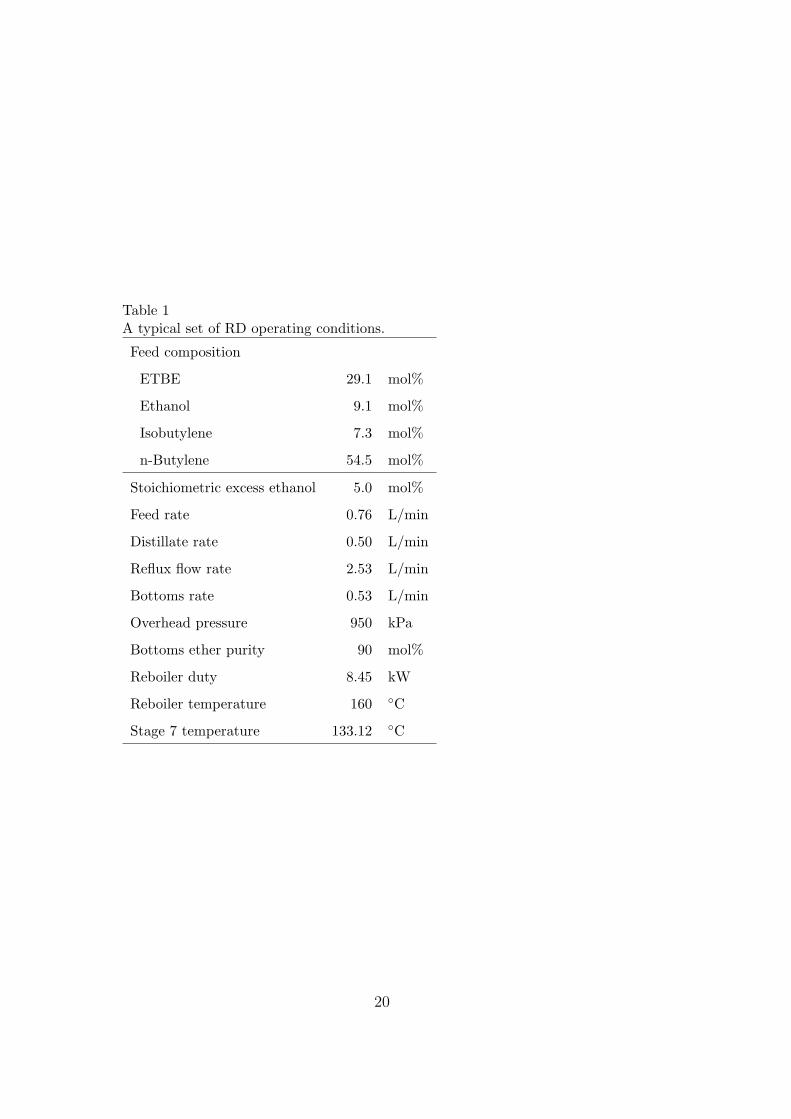
Table 1A typical set of RD operating conditions.

Feed composition

ETBE 29.1 mol%

Ethanol 9.1 mol%

Isobutylene 7.3 mol%

n-Butylene 54.5 mol%

Stoichiometric excess ethanol 5.0 mol%

Feed rate 0.76 L/min

Distillate rate 0.50 L/min

Reflux flow rate 2.53 L/min

Bottoms rate 0.53 L/min

Overhead pressure 950 kPa

Bottoms ether purity 90 mol%

Reboiler duty 8.45 kW

Reboiler temperature 160 ◦C

Stage 7 temperature 133.12 ◦C

20

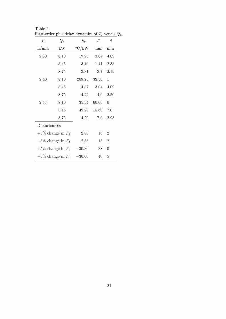
Table 2First-order plus delay dynamics of T7 versus Qr.

L Qr kp T d

L/min kW ◦C/kW min min

2.30 8.10 19.25 3.04 4.09

8.45 3.40 1.41 2.38

8.75 3.31 3.7 2.19

2.40 8.10 209.23 32.50 1

8.45 4.87 3.04 4.09

8.75 4.22 4.9 2.56

2.53 8.10 35.34 60.00 0

8.45 49.28 15.60 7.0

8.75 4.29 7.6 2.93

Disturbances

+5% change in Ff 2.88 16 2

−5% change in Ff 2.88 18 2

+5% change in Fc −30.36 38 0

−5% change in Fc −30.60 40 5

21

Table 3Fuzzy rules and degrees of fullfillment.

Ri IF THEN βi

R1 S4 is B r3 is S β1 = µ(S4 is S)

R2 (T/θ is not S) and (S4 is M) r3 is M β2 = min{1− µ(T/θ is S), µ(S4 is M)}R3 (T/θ is S) and (S4 is M) r3 is S β3 = min{µ(T/θ is S), µ(S4 is M)}R4 (T/θ is B) and (S4 is S) r3 is B β4 = min{µ(T/θ is B), µ(S4 is S)}R5 (T/θ is not B) and (S4 is S) r3 is M β5 = min{1− µ(T/θ is B), µ(S4 is S)}

22

Table 4Degrees of fullfillment and r3 for the RD purity control.

S4 ≤ 2.4 (2.4, 4.0] (4.0, 5.6] > 5.6

β1 = µ(S4 is S) 1 2.5− S4/1.6 0 0

β2 = µ(S4 is M) 0 S4/1.6− 1.5 3.5− S4/1.6 0

β4 = µ(S4 is B) 0 0 S4/1.6− 2.5 1

r3 V (S) β1V (S) + β2V (M) β2V (M) + β4V (B) V (B)

23

Table 5Comparisons of ITAE indices.

Magnitude Period Direct PI PPC Improve.

−5◦C step in T7 50-150min 657 479 27.1%

+2◦C ramp in T7 150-300min 434 313 27.9%

+5% step in Fc 50-150min 2529 1167 53.9%

−5% step in Fc 150-300min 2967 1175 60.4%

−10% step in Ff 50-300min 2461 1077 56.3%

+10% step in Ff 300-600min 2737 1210 55.8%

24

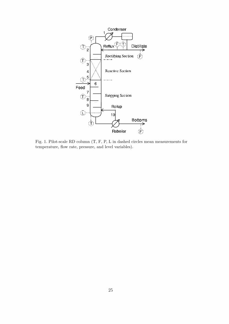
Fig. 1. Pilot-scale RD column (T, F, P, L in dashed circles mean measurements fortemperature, flow rate, pressure, and level variables).

25

7.5 8 8.5 940

50

60

70

80

90

100

Qr (kW)

Pur

ity &

Con

vers

ion

(%m

ol)

Purity Conversion

Fig. 2. Purity and Conversion versus reboiler duty for the reflux fixed at 2.53L/min.

26

6 7 8 9 1080

90

100

110

120

130

140

150

Qr (kW)

T7

(o C)

L = 2.30 L/minL = 2.40 L/minL = 2.53 L/min

Fig. 3. Stage 7 temperature T7 versus reboiler duty Qr.

27

Fig. 4. PPC system structure.

28

7.4 7.6 7.8 8 8.2 8.4 8.680

100

120

140

160

v

y (o C

)

y

7.4 7.6 7.8 8 8.2 8.4 8.67

8

9

10

11

u (k

W)

u

Fig. 5. Nonlinear transformation and the resulting y versus v relationship.

29

Time

Pro

cess

Res

pons

e

I II III IV

← A

Fig. 6. S-shape process response to a step change in either the manipunated variableor disturbances. I: time delay stage; II: accelerating increase stage; III: deceleratingincrease stage; IV: steady state stage; A: inflection point.

30

Fig. 7. Fuzzy sets and fuzzy rules.

31

0 50 100 150 200120

130

140

t (min)

y(t)

, y∧ (t

|t−dT

s) (o C

)

y

y∧

0 50 100 150 2008

8.5

9

v

v

Fig. 8. Typical curves of v, y, and y.

32

0 50 100 150 200−2

−1

0

1

2

t (min)

y(t)

− y

∧ (t|t−

dTs)

(o C)

y−y∧

0 50 100 150 2000

0.1

0.2

0.3

0.4

h

h

Fig. 9. Typical y(t)− y(t|t− dTs) and h curves corresponding to Figure 8.

33

0 50 100 150 200−0.5

0

0.5

1

1.5

t (min)

S1, 1

0S2

10S2

S1

0 50 100 150 200−5

0

5

10

15

S3, S

4

S4

S3

Fig. 10. Typical curves of S1 to S4 corresponding to Figure 8.

34

0 50 100 150 200 250 300127

128

129

130

131

132

133

134

t (min)

T7

(o C)

Setpoint PPC PI Direct PI

Fig. 11. Setpoint tracking.

35

0 50 100 150 200 250 300128

130

132

134

136

138

140

t (min)

T7

(o C)

Setpoint PPC PI Direct PI

Fig. 12. Rejection of ±5% disturbances in feed composition.

36

0 100 200 300 400 500 600132

133

134

135

t (min)

T7

(o C)

Setpoint PPC PI Direct PI

Fig. 13. Rejection of ∓10% disturbances in feed flow rate.

37