Participatory farm management

methods for analysis, decision making and

communication

Peter Dorward, Derek Shepherd and Mark Galpin

2007

Participatory farm management methods for analysis, decision making and communication

Section 1: THE DEVELOPMENT OF PARTICIPATORY FARM MANAGEMENT METHODS

1.1 Introduction

Participatory Farm Management methods are simple tools which enable farmers working on their own, or with research or extension workers, to explore their activities and the use and production of associated resources. The methods were developed by working closely with small-scale farmers in developing countries and have been successfully used in many countries for a range of purposes in research, extension and development. This document describes each of the methods i.e. Participatory Budgets, Scored Causal Diagrams, Resource Allocation Maps, Resource Flow Diagrams, and then provides examples of how they have been used. The uses include for: participatory extension and development (introducing new practices and considering how they compare to existing practices in terms of activities involved, timing, and the use and production of resources); needs assessment (identifying and understanding problems farmers face); assessing the suitability of potential interventions (establishing how appropriate interventions are for different farmers and systems and how they can be adapted before starting on-farm research or demonstrations); conducting on-farm participatory research (planning, recording and analysing results); adoption studies (clarifying why farmers have or have not adopted practices and what impact they have had) and; studying farmers’ practices and systems (e.g. research on farmers activities and use and production of resources). Recently there has been increasing interest in the application of participatory methods for larger scale studies and statistically based data analysis. The last section of the document considers this and presents some examples of scaling-up and analysis.

1.2 The development of participatory approaches

Farming Systems Research (FSR) emerged in the 1970s largely in response to the failure of conventional research and development approaches in developing countries. In particular it sought to move away from the single commodity focus and to adopt a more holistic approach to smallholder agriculture. FSR focuses on interdependencies between farm-household components under the control of household members, and on interactions between these components and the physical, biological and socio-economic factors not under the household’s control (Shaner, Philipp and Schmehl, 1982). Associated with this greater consideration of farmers’ actual conditions and circumstances, was increased integration of farmers into the research process and the emphasis on the perceptions and expectations of farmers regarding constraints confronting them. Typically this was elicited for a geographical area (recommendation

1

domain) and as part of detailed study of the farming system before identification of potential solutions.

Initially formal and extractive survey methods were used for needs assessment in FSR. However, this gave way to rapid, informal methods for data collection in the late 1970s, collectively termed Rapid Rural Appraisal (RRA) (Chambers, 1991). The development of RRA was largely due, according to Chambers (1997), to three main factors:-

i) Dissatisfaction with the anti-poverty biases of ‘rural development tourism’, i.e. spatial bias; project bias; person bias; diplomatic bias.

ii) Disillusionment with formal questionnaire surveys and their results which were viewed by many as: too focused; too long, expensive and difficult to administer and process; often giving inaccurate findings; often reported on late; and giving findings that are subsequently ignored.

iii) The need for cost effective learning, and increasing recognition by ‘professionals’ that rural people were highly knowledgeable about their own circumstances, systems and practices.

During the 1980s RRA was increasingly used and gained wider acceptance and credibility (Carruthers and Chambers, 1981). New methods were developed and added by individuals and institutions. In addition to the rapid, informal methods of data collection themselves, characteristics of RRA include its multidisciplinary, semi-structured and flexible sequence that is regularly reviewed and refined, and exploring local categories, classifications and perceptions (Cornwall, Guijt, and Welbourne, 1994).

Cornwall et al. (1994) notes that in RRA, multidisciplinary teams gathered, summarised and analysed information and although farmers generated data and discussed the teams’ findings, they were generally excluded from any analysis. RRA was therefore to an extent still an extractive process.

As part of a move towards more people-centred approaches in development (Scoones and Thompson, 1994) existing RRA methods began to be used in different ways and new ones were developed and added. These drew on findings on farmer’s capabilities and directly on new methods of analysis, emerging from development in action-reflection research, agroecosystems analysis, applied anthropology and studies of farmers’ experimentation. Chambers (1997) notes that in the mid 1980s the word ‘participatory’ entered the vocabulary

Participatory Rural Appraisal (PRA) has been defined as “a growing family of approaches and methods to enable local people to plan, act, monitor and evaluate” (Chambers, 1996).

Chambers (1993) identifies the main difference between PRA and RRA as being “whereas RRA is extractive, with outsiders appropriating and processing information, PRA is participatory, with ownership and analysis more by rural people themselves.” Greater emphasis is therefore given not just to rural peoples’ knowledge but to their

2

capacity to analyse, plan and act and to the process of enabling or ‘empowering’ people to take action. Consequently, the importance of the role of the outsider as a ‘facilitator’ is stressed in PRA, and much emphasis placed on his/her behaviour and attitudes. Mascarenhas et al.. (1991), therefore describes the three pillars of PRA as being ‘behaviour and attitudes’, ‘partnership and sharing’ and ‘methods’.

Regarding the methods used, Cornwall et al. (1994) note that “RRA and PRA make use of a rich menu of visualisation, interviewing and groupwork methods of which visualisation has proved particularly innovative in agriculture”. PRA / RRA methods commonly used1 include mapping, timelines, matrix scoring and seasonal calendars. Full descriptions of methods and examples of their use are well documented in the literature, including PLA notes, and in manuals / resource books e.g. Pretty, Guijit, Thompson and Scoones (1995).

RRA / PRA methods are therefore generally used by and with participants and facilitated by an outsider and can be applied for either research and / or development purposes. The term Participatory Learning and Action (PLA) became more widely used than PRA / RRA in recognition that participatory approaches are not limited to rural areas or the process of appraisal as suggested by the term PRA. Results from PLA activities are often used to draw findings and conclusions with participants and for their particular location. Often this meets the objective of the exercise e.g. for a community to identify opportunities and constraints and initiate activities to address some of them. Recently there has been increased interest in applying PLA methods in a way that will allow quantitative analysis e.g. to combine results from exercises repeated with other participants at the same location, or to compare and analyse results from different locations.

1.3 Farm management and the development of Participatory Farm Management Methods

Farm management is a process of decision-making, which involves the evaluation and implementation of alternative farming strategies. Farm management is therefore essentially a decision-making process involving the identification and evaluation of alternative production strategies (Harding, 1982). Farm management methods are consequently means of assisting farmer’s decision-making. Normally this is by quantifying and analysing the use of resources on a farm, and by presenting possible outcomes and consequences of different decisions. Farm management methods are then “a formal method or procedure that is employed to generate information used by a decision- maker to analyse and specify possible solutions to his problems and / or monitor and evaluate the progress and effectiveness of a solution that was chosen and implemented” (Rehman and Dorward, 1984).

Examples of common conventional farm management methods include enterprise budgets, whole farm budgets, gross margins, profit and loss accounts, balance sheets,

1 Most methods can be used for either RRA or PRA, depending on the aims and approach of the facilitator, although the more visual encourage active participation.

3

cash flows, partial budgets and labour profiles. They are used widely by farmers in the North and by commercial farmers throughout the world for a variety of purposes including to:

Plan activities and resource and finance implications

Compare the performance and implications of alternative strategies before deciding which to implement

Predict the effects of potential changes in practices and inputs (both those that are under the control of the manager and those that are not e.g. prices)

Monitor performance against plans and identify action to take in response to changes

Monitor and evaluate performance against previous seasons' performances and other businesses and identify areas where changes can be made to improve the business.

More complex methods such as linear programming and other decision making models have generally been used in research and policy development, but little by farmers themselves. Nevertheless research in farm management has tended to focus on these in recent decades and less on methods or topics of direct benefit to farmers (Dorward, Shepherd and Wolmer, 1997).

The majority of the worlds' farmers are small-scale farmers in developing countries and operating in diverse and high risk conditions. Despite concerted efforts by government and international organisations over several decades to introduce 'conventional' farm management methods, they are little used by such farmers or their advisers.

Consultation and discussion with those involved in agricultural research and extension in developing countries and a review of relevant literature were undertaken (Dorward et al., 1997). It was concluded from this that the underlying concepts of farm management were useful to small-scale farmers but that the existing farm management methods were largely inappropriate for the following reasons:

1 Conventional farm management methods focus on a specific financial aspect of a farm or enterprise, for example, profit, cash, or worth and ignore other resources. They assume farmers’ motives are to maximise profit or improve financial performance. However small-scale farmers operating in complex, diverse and risk-prone environments often have multiple objectives (including food security) and are often more interested in trying to minimise risk. Small-scale farmers are therefore interested in, and limited by, a range of resources, not just cash e.g. food stocks, complementary fodder production.

2 Conventional farm management methods do not generally take account of changes over time (e.g. over a season) but look at the end result (e.g. a profit or a

4

loss at the end of the season / year). However small-scale farmers’ resources do vary considerably over time both within and between seasons, and this may be more important to farmers than the ‘end’ result at the end of the season. For example, cash may be particularly limiting in a certain month because school fees need to be paid. This will affect the feasibility of farmers undertaking an enterprise which needs an injection of cash at this time, however ‘profitable’ the enterprise may be. Furthermore, farmers often take decisions during a season, depending on conditions at that point (e.g. how good the rains have been, how much labour is available) and not simply before its start.

3 Conventional farm methods are complex and difficult to use, particularly for non or semi-literate farmers with little or no formal education and who can amount to 60% or more of the rural population in many parts of the world. Where conventional farm management methods have been used in smallholder agriculture, it has been by researchers extracting or eliciting information from farmers which is then analysed using farm management methods. The complexity of the methods prevents farmers from using them, or from outsiders using them in a collaborative or participatory way with farmers.

4 Due to their complexity, conventional methods often require support equipment such as personal calculators or even computers which are not available to small-scale farmers. Even equipment such as pens and paper may be unavailable and can alienate non or semi-literate farmers.

A project was commissioned by the UK department for International Development (DFID)2 to develop, test and disseminate appropriate methods. The project was led by the University of Reading who worked in collaboration with AGRITEX and Research and Specialist Services in Zimbabwe and the Ministry of Food and Agriculture in Ghana.

A set of Participatory Farm Management (PFM) methods was developed (which are described in section 2). These draw on lessons and concepts from both farm management and participatory approaches. The emergence of PLA had demonstrated peoples’ abilities to rank, score, diagram and map, irrespective of their literacy level. Furthermore the emphasis of PLA on visualisation, and analysis and ownership of information by farmers provided a good basis from which to develop appropriate methods that specifically sought to address the limitations of conventional farm management methods outlined above. PFM methods have to date been used by or with farmers for a range of uses and for a variety of purposes in many countries.

1.4 Further uses of PFM methods

Participatory methods have been widely used in local and site specific studies and development interventions (for examples of their use see section 3). There is increasing demand for using the information generated in participatory interactions in ways which

2 This work was funded by the UK Department for International Development’s Natural Resources Division under project R6730.

5

allow these data to be compared and aggregated for higher level planning and policy purposes.

Chambers (2003) for example, refers to three ways participatory activity can generate numbers, for different purposes and with different levels of ownership by local people.

o Analysis of secondary data which have been generated in a participatory manner without standardisation. In this mode the numbers belong to the outsiders.

o Participatory monitoring and evaluation in which local people identify their own indicators, including qualities that are scored and quantities that are measured, and the monitor them. This is a more empowering mode in which the numbers belong more to local people.

o Numerical data from several sources generated using participatory approaches, methods and behaviours which are to some degree standardised and predetermined. In this case ownership will vary depending on context and facilitation.

PFM methods enable the quantification of resources such as crop inputs thereby making some form of quantitatively based analysis of information possible. Experience of their use to date suggests that this provides an opportunity for collation and analysis within a site specific context, both in research and development contexts. However, their use as elements of more extensive quantitative investigation above the community level would require them to be used in a way which allowed for the standardization and comparability required for the application of statistical tools. This is considered further in the final section. The next section describes PFM methods in detail.

6

Section 2 PARTICIPATORY FARM MANAGEMENT METHODS

2.1 Introduction

Participatory Farm Management Methods are simple tools which enable farmers, working on their own or with a facilitator, to quantify and analyse the use and production of resources at the farm or household level and to present different decision outcomes. They can be used for a variety of purposes which include exploring the resource implications of making a change to an enterprise or farming system and comparing different enterprises with each other. This section describes four methods, with examples, and how they can be used.

• Participatory Budgets are tools which examine a farmers’ use and production of resources over time for a particular enterprise

• Resource Allocation Maps examine the use of resources over the whole farm during a specific period of time (e.g. a month, season)

• Resource Flow Diagrams help to analyse flows of resources within a farm / household and with the external environment

• Scored Causal Diagrams help to examine in detail the causes and effects of problems experienced by farmers and identify and prioritise causes which have most impact and need to be addressed.

The methods have been used widely with small-scale farmers in developing countries. Central to the successful use of PFM methods is the fact that the farmer is the decision maker i.e. he or she takes the risks associated with decisions made. Similarly, as with all PLA, the attitude of the facilitator i.e. as ‘learners’ and not ‘experts’, is crucial and training in PFM should include the development in facilitation skills. The methods were designed with a collegiate interaction between adviser and farmer in mind, and not as tools to assist in the promotion of particular technologies or strategies.

This section of the chapter draws heavily on a manual on PFM methods (Galpin, Dorward and Shepherd, 2000) where further details on and examples of uses of the methods can be found.

2.2 Participatory Budgets (PBs)

2.2.1 Introduction

Participatory budgeting is a method which allows farmers and outsiders to quantify and analyse resource inputs and outputs over time for a particular enterprise, or for a particular resource over the whole farm. This method is based on a traditional African board game generically known as mancala (tsoro in Zimbabwe and oware in Ghana), and builds on farmers’ abilities to play this essentially mathematical game, together with their ability to rank, score and construct seasonal diagrams which has been

7

demonstrated in PLA activities. The method seeks to enable analysis and planning and is easy to use. They can take account of non-cash resources, they look at resource use over time, and they are implemented using readily available local materials. The method can be used with individual farmers, or with a group of farmers where one is acting as a case-study. Alternatively, an ‘average’ budget can be made up for a given size of enterprise, if all the farmers in the group have similar characteristics in terms of their production practices and available resources.

Participatory Budgets (PBs) are tools which examine a farmer’s use and production of resources over time for a specific enterprise. Their main uses are for:

• analysing farmers existing and past activities, resource-use and production

• exploring the resource implications of making a change to an enterprise

• comparing different enterprises

• planning a new enterprise

2.2.2 Description of Participatory Budgets

A PB is essentially a board or grid drawn on the ground on which time is represented by each column as a month, week, day or other period of time. The first column is therefore the first month, the second the second month etc. Activities for each time period are indicated in the top row, using symbols. The types of resources are indicated by different types of symbols e.g. beans / counters in different rows on the board or grid. Quantities of resources are indicated by the number of beans / counters, with a value attached to each one.

8

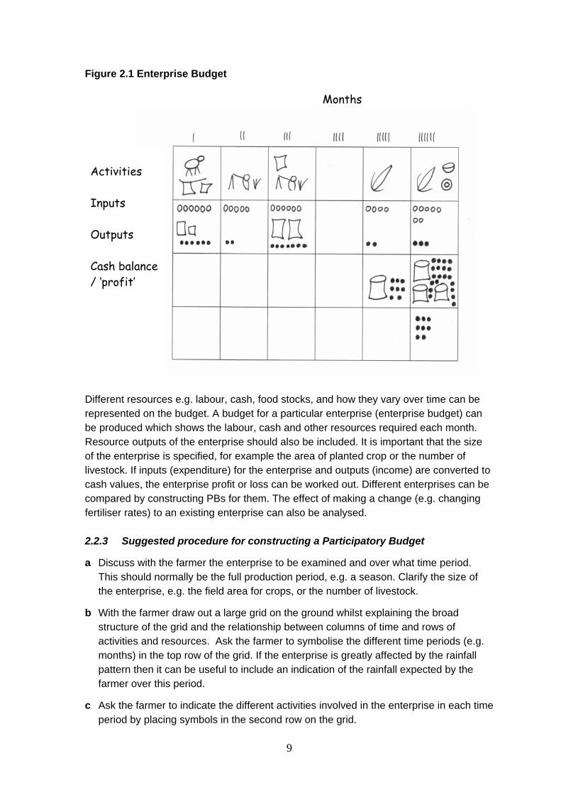
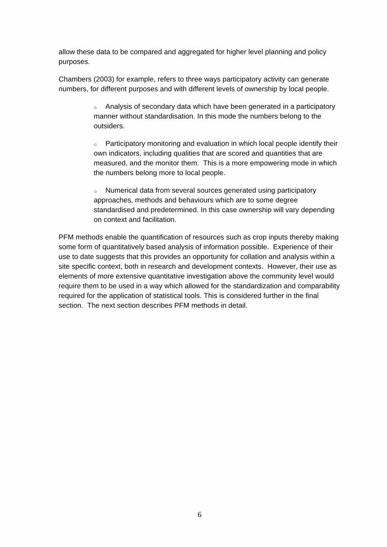
Figure 2.1 Enterprise Budget

Months

Activities Inputs Outputs Cash balance / ‘profit’

Different resources e.g. labour, cash, food stocks, and how they vary over time can be represented on the budget. A budget for a particular enterprise (enterprise budget) can be produced which shows the labour, cash and other resources required each month. Resource outputs of the enterprise should also be included. It is important that the size of the enterprise is specified, for example the area of planted crop or the number of livestock. If inputs (expenditure) for the enterprise and outputs (income) are converted to cash values, the enterprise profit or loss can be worked out. Different enterprises can be compared by constructing PBs for them. The effect of making a change (e.g. changing fertiliser rates) to an existing enterprise can also be analysed.

2.2.3 Suggested procedure for constructing a Participatory Budget

a Discuss with the farmer the enterprise to be examined and over what time period. This should normally be the full production period, e.g. a season. Clarify the size of the enterprise, e.g. the field area for crops, or the number of livestock.

b With the farmer draw out a large grid on the ground whilst explaining the broad structure of the grid and the relationship between columns of time and rows of activities and resources. Ask the farmer to symbolise the different time periods (e.g. months) in the top row of the grid. If the enterprise is greatly affected by the rainfall pattern then it can be useful to include an indication of the rainfall expected by the farmer over this period.

c Ask the farmer to indicate the different activities involved in the enterprise in each time period by placing symbols in the second row on the grid.

9

d Discuss with the farmer which resources are used and are important e.g. labour, cash, manure. Identify different counters to represent each of these.

e For the first resource selected, identify the units the farmer uses to measure this resource. For example fertiliser may be indicated by number of bags, and labour by number of people and number of days. Ask the farmer to indicate the quantity of that particular resource required in each month, by placing a specific number of beans / counters in each column of the next row of the grid. Referring to the activities row will help with this.

f Repeat step (e) for each of the resources the farmer wants to include on the PB.

g In the same way indicate the outputs and income that the farmer will receive from the enterprise, including any by-products e.g. fodder.

h If the farmer is interested in the ‘end balance’ of resources, this can be worked out by comparing resources used (expended) and products received (income). It is important that all the outputs and inputs of the enterprise are included in this and not just those given cash values. Therefore the ‘end balance’ may be expressed as; 3 bags of maize and $100 cash. Or, if a cash loss is made; 3 bags of maize less $100 cash. More commercially orientated farmers may want to convert all resources into cash terms and calculate ‘profit’. The facilitator needs to ensure that the exercise does not get side-tracked into just considering money. Although PBs can be used to predict or record ‘profitability’, their primary purpose is to enhance understanding about resource allocation options and decision-making. All resource inputs and outputs that the participants consider to be important should be included.

i To identify what the potential risks are to the enterprise ’what if’ questions can be asked. It is advisable to concentrate on those phenomena that are most likely to happen. For example, if it is a rain-fed crop what would be the effect of the rains arriving late or a change in input prices? Ask the farmer to indicate the effect of different scenarios on the budget. By examining enterprises or new innovations under different scenarios the ‘robustness’ of the enterprise or technology can be examined.

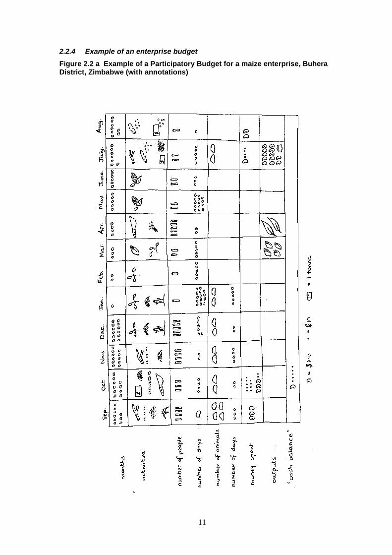
Figures 2.2 a and 2.2 b below show an example of an enterprise Participatory Budget. This Participatory Budget was constructed by a group of women farmers in Buhera District, Zimbabwe. The budget shows the resource outputs and inputs for 1 acre of maize. When constructing the budget, symbols and counters were used on the ground. These have been interpreted for ease of explanation in the next figure. All labour used was family labour and the farmers chose not to cost this. All the produce was sold. Cash figures are given in Zimbabwe dollars.

10

2.2.4 Example of an enterprise budget Figure 2.2 a Example of a Participatory Budget for a maize enterprise, Buhera District, Zimbabwe (with annotations)

11

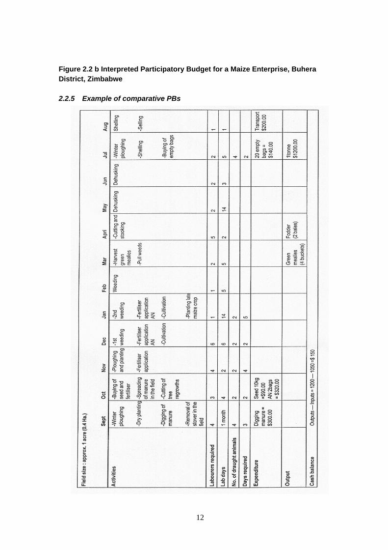
Figure 2.2 b Interpreted Participatory Budget for a Maize Enterprise, Buhera District, Zimbabwe

2.2.5 Example of comparative PBs

12

An adaptation to the Participatory Budget is the comparative PB which is used to either compare one enterprise with another (e.g. groundnuts with sunflower) or to compare changes to an existing enterprise (e.g. use of organic or inorganic fertilisers). To construct a comparative PB, PBs must be produced for the existing enterprise and the changes. These can be presented as two separate budgets or incorporated into one as in the following example.

In the following example farmers in Buhera District, Zimbabwe compared the two main cash crops grown in their area, sunflower and groundnuts. The budget illustrates the resources required for the two crops and their ‘profitability’. Visualising the farmers’ knowledge in this form clarified and summarised the differences between the two crops for them. The process of constructing the budget also assisted communication between the facilitator and farmers, particularly regarding what factors influence farmers choices between the two crops. All the farmers were enthusiastic about the exercise and keen to repeat it for different enterprises.

Figure 2.3 Comparative Participatory Budget for groundnut and sunflower crops, Buhera District, Zimbabwe

13

Photograph 2.1 Farmers constructing a Participatory Budget for sunflower and groundnuts, Buhera District, Zimbabwe

2.3 Scored Causal Diagrams (SCDs)

2.3.1 Introduction

Problem listing, scoring and ranking are commonly used and effective PLA tools. However these often fail to examine the relationships between the problems identified, as scores are given for each problem independently, even if the problems are closely linked. This can result in closely related problems being seen in isolation. Attempts have been made to look at these inter-relationships e.g. using problem tree analysis, however this is often a method used purely for the collection of information, with analysis and interpretation carried out by outsiders rather than the community themselves.

Causal diagramming is a technique which helps the farmer and researcher together to identify the linkages and relationships between different problems. This technique has begun to be used by PLA practitioners and is further developed in this document, mainly through the introduction of a scoring method which is used with the diagram.

14

Scored Causal Diagrams (SCDs) are particularly useful when discussing the problems associated with a specific crop or enterprise. However, they can also be used to look at

es

scoring technique is introduced. Such a method is much easier to use in the field, than it is to

parent

l Diagrams

d to be a ‘definitive statement’ but as a useful tool to aid discussion and in-depth analysis of problems and issues together with

e noted that individual problems are often causes of other problems. It is therefore artificial to distinguish between problems and causes. In the text we therefore

more general problems facing an individual or a community as a whole. Although not strictly a PFM method, as they do not explore quantities of resources, SCDs are includedhere as they were developed in association with PFM methods in order to identify issuto focus on and investigate and have proved very useful tools for this.

In this section, Causal Diagrams (CDs) are first described and then the

describe. We would therefore encourage those who are put-off initially by the apcomplexity of SCDs to persevere and have a go in the field, as this is when their strengths become apparent.

2.3.2 Description of Causa

A Causal Diagram should not be considere

farmers.

It should b

use the terms interchangeably.

Scored Causal Diagrams help to examine in detail the causes and effects of problems and to identify the ‘root’ causes which need to be addressed. The scoring procedure helps to analyse the relative importance of the problems and prioritise them.

15

Photograph 2.2 Farmers constructing a Causal Diagram, Brong Ahafo Region, Ghana

2.3.3 Suggested procedure for constructing a Causal Diagram

a The topic or area of discussion is first identified with the participants. This could be simply ‘general’ problems facing a community or could be focused on a specific crop or enterprise which interests the participants.

b The farmers discuss and list their problems using symbols to illustrate each problem as it is identified. This list is then scored. The facilitator explains that often problems are connected and the next step is to look at the connections between the problems identified. This can be explained briefly using an appropriate example.

c If a specific enterprise is being discussed, the objective of the enterprise needs to be clarified with the participants by asking why they are involved in this particular enterprise. For example, if it is a cash crop the objective is likely to be to ‘earn income’. If it is a food crop it is likely to be to ‘grow enough food to eat’. Often there may be more than one objective, for example for a crop which is both eaten and sold. All objectives should be identified.

d These objectives (or objective) are then expressed as problems and symbolised on the ground. For example, if tomatoes were being discussed and the objective of the farmers was to ‘earn an income from tomatoes’, this objective expressed as a problem becomes ‘low income from tomatoes’. If the objective is ‘enough tomatoes to eat’ this becomes ‘not enough tomatoes to eat’. On a ‘general’ Causal Diagram the objective is likely to be ‘wealth’ or ‘happiness’. The end problem would therefore be

16

‘poverty’ or ‘unhappiness’. The objective expressed as a problem is the ‘end’ or final problem on the Causal Diagram which all other problems eventually cause.

e The direct causes of the ‘end’ problem are then identified by the farmers. As they are identified the symbols are placed on the diagram and arrows are drawn in to represent the causal relationships between the problems. Each problem is represented on the ground once only. The causes of those problems are identified and added to the diagram. These may be from the original list or may be newly identified. The process is continued until the participants are happy that all the problems have been included and all the connections identified.

N.B. It is important that a general ‘lack of money’ as a cause, is separated from the problem of ‘low income from the enterprise’, otherwise it can result in a very confusing diagram. It is normally best to exclude the problem of a general ‘lack of money’ altogether from the diagram as it can dominate and be seen as the source of all the problems.

f The problems at the edge of the diagram with no identified ‘causes’ are the ‘root’ causes. If the logic of the diagram is correct, solving these ‘root’ causes will result in the other problems being overcome. It can therefore be useful to discuss possible solutions to these ‘root’ causes with farmers and identify which ones can be influenced by the farmers themselves, and which cannot. Those which are outside of the control of the farmer may be researchable or policy constraints which need outside support to overcome. Researchers should investigate these problems further. For example ‘poor rainfall’ may be overcome by a more appropriate crop variety or through water conservation measures. Other problems which can be influenced by the farmers are likely to be ‘developmental’ in nature and subject to more immediate influence.

g The positive effects of the solution can be traced back on the diagram, turning problems into solutions e.g. ‘insufficient food to eat’ becomes ‘sufficient food to eat’.

h Constructing a CD can result in the farmers prioritising the possible solutions which they would like to explore further.

2.3.4 Example of a Causal Diagram for a specific enterprise

The following example is from an exercise carried out with a group of farmers in Buhera District, Zimbabwe who specialise in cotton growing. The problems associated with cotton production were discussed and a Causal Diagram of these problems drawn up.

17

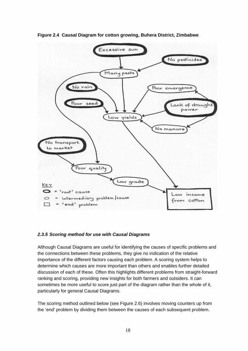
Figure 2.4 Causal Diagram for cotton growing, Buhera District, Zimbabwe

2.3.5 Scoring method for use with Causal Diagrams

Although Causal Diagrams are useful for identifying the causes of specific problems and the connections between these problems, they give no indication of the relative importance of the different factors causing each problem. A scoring system helps to determine which causes are more important than others and enables further detailed discussion of each of these. Often this highlights different problems from straight-forward ranking and scoring, providing new insights for both farmers and outsiders. It can sometimes be more useful to score just part of the diagram rather than the whole of it, particularly for general Causal Diagrams.

The scoring method outlined below (see Figure 2.6) involves moving counters up from the ‘end’ problem by dividing them between the causes of each subsequent problem.

18

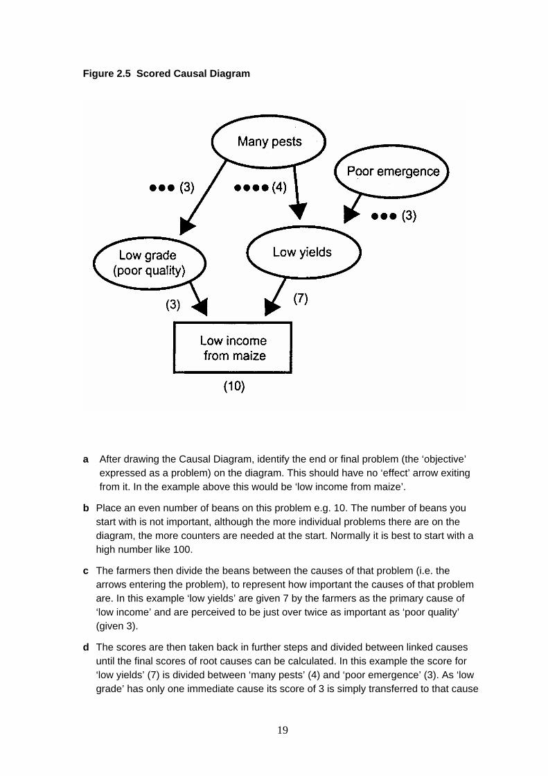
Figure 2.5 Scored Causal Diagram

a After drawing the Causal Diagram, identify the end or final problem (the ‘objective’ expressed as a problem) on the diagram. This should have no ‘effect’ arrow exiting from it. In the example above this would be ‘low income from maize’.

b Place an even number of beans on this problem e.g. 10. The number of beans you start with is not important, although the more individual problems there are on the diagram, the more counters are needed at the start. Normally it is best to start with a high number like 100.

c The farmers then divide the beans between the causes of that problem (i.e. the arrows entering the problem), to represent how important the causes of that problem are. In this example ‘low yields’ are given 7 by the farmers as the primary cause of ‘low income’ and are perceived to be just over twice as important as ‘poor quality’ (given 3).

d The scores are then taken back in further steps and divided between linked causes until the final scores of root causes can be calculated. In this example the score for ‘low yields’ (7) is divided between ‘many pests’ (4) and ‘poor emergence’ (3). As ‘low grade’ has only one immediate cause its score of 3 is simply transferred to that cause

19

(‘many pests’). The final root cause scores will therefore be ‘many pests’ 7 (3+4) and ‘poor emergence’ 3.

e On completion of the scoring process, the relative scores of the ‘root’ causes can be compared. The higher the score the more important the problem. This helps the farmers to prioritise the problems which require action. These scores and the reasoning behind the scores (i.e. the causes and effects on the diagram) should be clarified with the participants and solutions discussed.

f It can be useful to get different ‘categories’ of farmers to score the same diagram. These categories may be defined by the way they produce a particular crop or different wealth, gender or age groups could be used. This highlights the differences between the priorities and problems facing these different categories of farmers.

2.3.6 Scored Causal Diagram: example from Zimbabwe

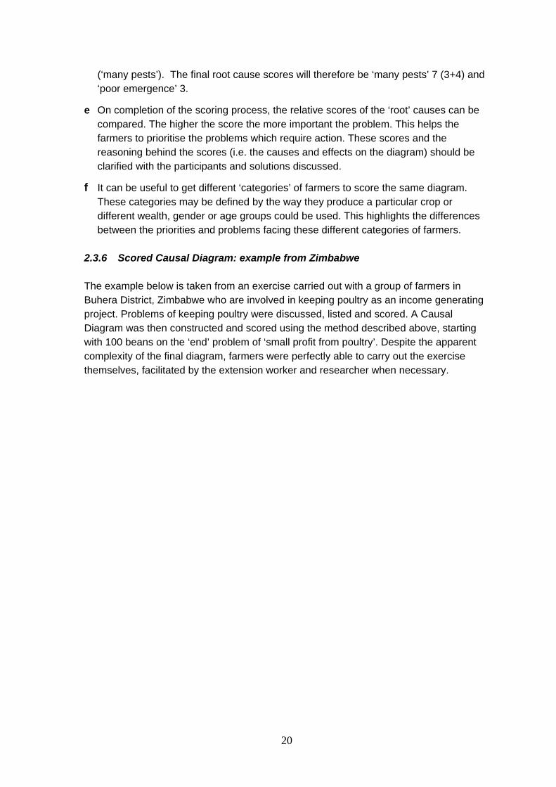
The example below is taken from an exercise carried out with a group of farmers in Buhera District, Zimbabwe who are involved in keeping poultry as an income generating project. Problems of keeping poultry were discussed, listed and scored. A Causal Diagram was then constructed and scored using the method described above, starting with 100 beans on the ‘end’ problem of ‘small profit from poultry’. Despite the apparent complexity of the final diagram, farmers were perfectly able to carry out the exercise themselves, facilitated by the extension worker and researcher when necessary.

20

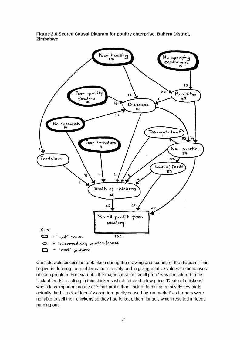
Figure 2.6 Scored Causal Diagram for poultry enterprise, Buhera District, Zimbabwe

Considerable discussion took place during the drawing and scoring of the diagram. This helped in defining the problems more clearly and in giving relative values to the causes of each problem. For example, the major cause of ‘small profit’ was considered to be ‘lack of feeds’ resulting in thin chickens which fetched a low price. ‘Death of chickens’ was a less important cause of ‘small profit’ than ‘lack of feeds’ as relatively few birds actually died. ‘Lack of feeds’ was in turn partly caused by ‘no market’ as farmers were not able to sell their chickens so they had to keep them longer, which resulted in feeds running out.

21

As the inter-relationships were identified and discussed, the exact nature of the problems were clarified. For example, for the problem of ‘no market’ it was crucial to determine what this meant and why there was ‘no market’. It transpired that healthy chickens sold well, and there was only a problem of ‘no market’ if your chickens were unhealthy. This highlighted the need for disease and parasite control and therefore good housing and equipment. A farmer suggested that the ‘no market’ problem could also be reduced if production was timed to coincide with peak demand, e.g. Christmas.

Photograph 2.3 Scoring of poultry Causal Diagram

22

2.4 Resource Allocation Maps (RAMs)

2.4.1 Introduction

Resource Allocation Maps (RAMs), like Participatory Budgets, also examine resource use. However, they look at the whole farm in a single time frame (e.g. a month), rather than at an individual enterprise over time. RAMs can easily be combined and used together with Participatory Budgets as planning and recording tools.

Resource Allocation Maps (RAM) examine the use of resources over the whole farm during a specific period of time e.g. a month. RAMs can be used for:

• looking at farmers’ decisions regarding resource allocation in different situations.

• examining resource competition between different enterprises at a specific time of the year

2.4.2 Description of Resource Allocation Map

This method builds on the PLA technique of mapping and incorporates an analysis of the quantities of resources used on a particular farm. The different resources which can be manipulated or controlled by the farmer are represented by different types of beans, seeds or counters. These counters are placed onto a map of the farm to indicate the amount of that resource invested in that field or part of the farm in the time period under discussion. Outputs can also be included on the map using different types of counters.

Resource Allocation Maps can also be adapted and combined with Participatory Budgets for record keeping and for long-term needs assessment exercises by comparing farmers planned and actual activities and resource use. RAMs can also be combined with Resource Flow Diagrams (RFDs) to analyse the flows of resources on the farm.

2.4.3 Suggested procedure for constructing a RAM

a Ask farmers to draw a map of their own farm indicating all the different fields and agricultural activities that they are involved in. This can be done individually or in groups of two or three, all of whom should know the farm reasonably well.

b Discuss with farmers the different resources which they have control over, and how much of each resource is used in each field / activity over a specific time period (eg the week, month or year).

c Ask the farmers to place counters on the different fields and enterprises on their map to represent the different amounts of resources used on them over the specified time period. The units used for each resource and the value of different counters should be decided by the farmers.

23

d Repeat this for the outputs from each field or enterprise on the farm.

e Discuss the results with the farmers, clarifying with them anything which appears unclear.

f Discuss different situations that might affect the type of enterprises and allocation of resources e.g. predicted rainfall, crop prices, and ask the farmers to then alter their RAM to indicate what changes they would make in these situations.

g Discuss the changes they have made to the RAM and the reasons for these changes.

2.4.4 Resource Allocation Map: example from Zimbabwe

The following example is from an exercise undertaken on a specific farm in Buhera District, Zimbabwe with the farmer and a group of his neighbours.

The participants first drew a map of the farm indicating all the different enterprises and activities during the previous growing season. The farmers then chose to look at the use of cash, labour and manure over the growing season on the farm. When the initial RAM was completed, the facilitator asked how the resource allocation would have changed if the farmer had been experiencing a drought year. The group then adapted the RAM to reflect these changes, as illustrated below.

24

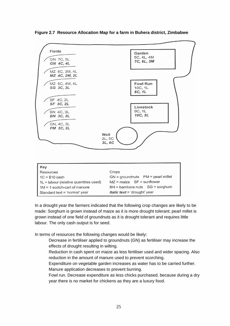
Figure 2.7 Resource Allocation Map for a farm in Buhera district, Zimbabwe

In a drought year the farmers indicated that the following crop changes are likely to be made: Sorghum is grown instead of maize as it is more drought tolerant; pearl millet is grown instead of one field of groundnuts as it is drought tolerant and requires little labour. The only cash output is for seed.

In terms of resources the following changes would be likely: Decrease in fertiliser applied to groundnuts (GN) as fertiliser may increase the effects of drought resulting in wilting. Reduction in cash spent on maize as less fertiliser used and wider spacing. Also reduction in the amount of manure used to prevent scorching. Expenditure on vegetable garden increases as water has to be carried further. Manure application decreases to prevent burning. Fowl run. Decrease expenditure as less chicks purchased, because during a dry year there is no market for chickens as they are a luxury food.

25

Livestock. Increase cash as he buys fodder for animals. Decrease in the number of livestock to reduce risk, and an increase in labour input with the need to cut fodder from further away. Well. Increase cash input for deepening well.

2.5 Resource Flow Diagrams (RFDs)

Resource Flow Diagrams (RFD) were originally developed by Clive Lightfoot (Lightfoot, De Guia, Aliman and Ocado,1989) and have been widely used particularly by ICLARM in S.E. Asia, Malawi and elsewhere to analyse flows of resources in aquacultural and agricultural systems. They can be combined with Resource Allocation Maps and are a useful technique for looking at resource flows at the farm level.

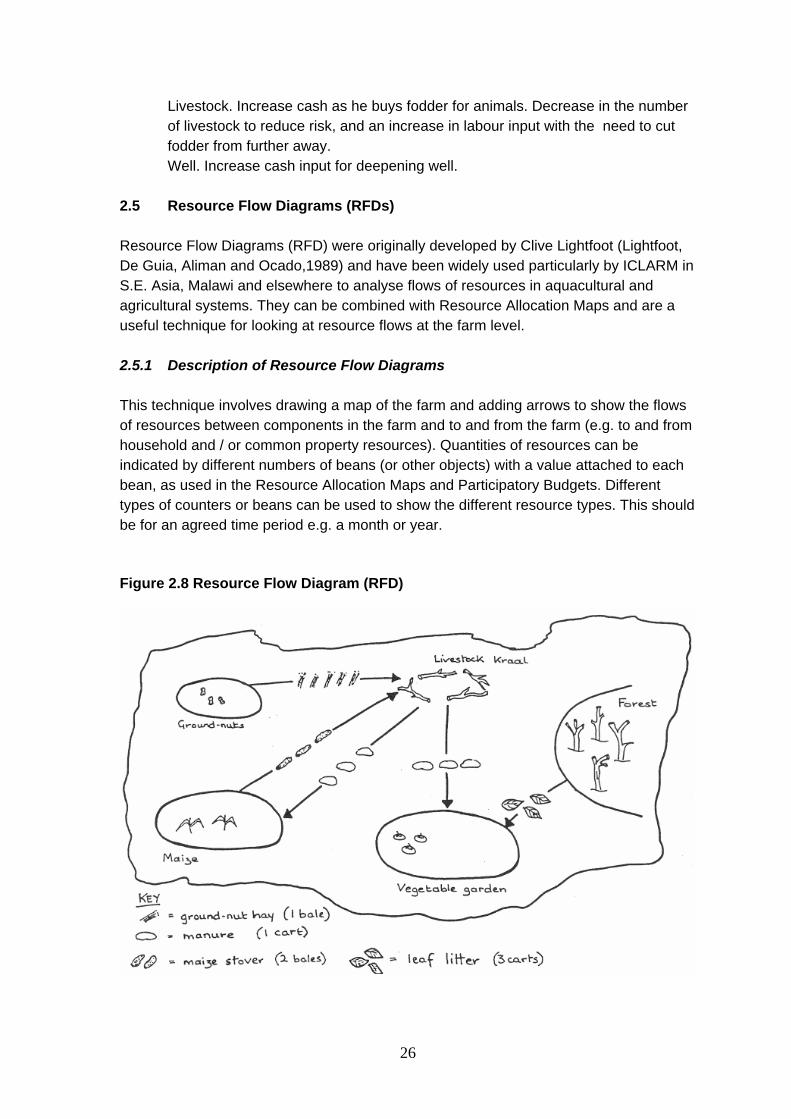
2.5.1 Description of Resource Flow Diagrams

This technique involves drawing a map of the farm and adding arrows to show the flows of resources between components in the farm and to and from the farm (e.g. to and from household and / or common property resources). Quantities of resources can be indicated by different numbers of beans (or other objects) with a value attached to each bean, as used in the Resource Allocation Maps and Participatory Budgets. Different types of counters or beans can be used to show the different resource types. This should be for an agreed time period e.g. a month or year.

Figure 2.8 Resource Flow Diagram (RFD)

26

2.5.2 Suggested procedure for constructing a RFD

a Identify major components of the farm and map them on the ground using local materials.

b Identify a resource which the farmer considers important. Discuss how this resource moves between different parts of the farm and draw these flows on the farm map e.g. manure from kraal to maize field.

c Determine what units the farmer uses to quantify the resource.

d Indicate next to each arrow the quantities of resources involved in each of the flows by placing beans or counters next to the arrows.

e Repeat steps b) to d) for other resources on the farm.

f Identify additional flows of resources on (and from) the farm and draw them on the map.

g Introduce different scenarios (What if’s …?) and assess their immediate and knock-on effects on the farm as a whole, using the resource flow diagram.

2.5.3 Uses of RFDs

Resource Flow Diagrams (RFDs) help to examine the movement of resources around the farm and with outside it. They are particularly useful for assessing the wider impact of a change to a specific part of the farming system. For example, if a new enterprise is undertaken, what resources will it require and how will this impact on the other enterprises on the farm which compete for those resources? How will the introduction of a new technology affect these resource flows and the rest of the farming system? If flows of resources onto and away from the farm are included on the diagram the impact of changes in the external environment can also be assessed.

RFDs have also been used to assess the sustainability and performance of farming systems using the indicators of bio-diversity (number of enterprises), input-output balance, efficiency, and recycling (number of bio-resource flows) (Lightfoot, Dalsgaard and Bimbao, 1993).

27

SECTION 3: USES OF PFM METHODS

3.1 Introduction Participatory Farm Management methods can be used for a variety of purposes. This section outlines some of the ways that PFM methods have been used by drawing on our and others experiences from Ghana, Zimbabwe, Kenya and Uganda. These examples are largely limited to the use of the methods in agricultural research and extension. However, the methods might easily be used in the wider context of ‘development’. Participatory Budgets for example can be used throughout the development process for planning, implementation, monitoring and evaluation for enterprises. Figure 3.1 illustrates different stages in the processes of research and intervention and where PFM methods can be used. Figure 3.1. Diagrammatic representation of the research - extension process and the potential role of PFM methods

Needs assessment: 1. Identification of

constraints (PLA + PFM) 2. Identification of possible

solutions

Assessment of Suitability of Potential Innovations / possible solutions (PBs, CDs, RAMs)

Planning of research: - design of on-farm trials

etc. (PBs)

Implementation and monitoring of on-farm trials

(PBs)

Evaluation of tech. from OFT (PBs)

Further on-farm research and trials (PBs)

Farmer-to farmer Extension / (PBs)

Dissemination

4.‘Adoption and use processes’

2. ‘Suitability Assessment’

1.Needs Assessment

3. On-Farm trials / experimentation

28

3.2 ‘Needs assessment’ and ‘suitability assessment’ The term ‘needs assessment’ generally refers to the use of participatory tools and methods to diagnose and prioritise (researchable) constraints together with farmers and other stakeholders. Usually this is for a specific geographical area and often it is conducted in respect to a specific topic e.g. post-harvest issues. PFM can be used in one-off or short-term needs assessment activities frequently practised at the beginning of a project, using a range of participatory tools, to define the current situation and identify constraints. Alternatively they can be used in longer-term processes that involve participatory interaction with clients over extended periods (e.g. several weeks or months). This enables more thorough understanding of the dynamics of systems and helps avoid particular biases that could result from single one-off investigations. An additional step to needs assessment is required prior to conducting on-farm research. This involves assessing the suitability, or ‘screening’, of potential innovations or solutions to the problems identified (see Fig. 3.1 above). We have referred to this stage as ‘suitability assessment’. For example, if poor soil fertility is identified as a problem, an assessment of the suitability of potential solutions to this constraint (e.g. fertiliser, green manures, compost), is necessary prior to the commencement of on-farm research. This should help ensure the appropriateness of the innovation being examined in terms of farmers’ resources and the system as a whole. Currently, this is a stage which is either left out, or is carried out by research staff with little or no input from farmers. When it is carried out, socio-economic factors and resource issues are rarely considered. PFM offers methods which enable this preliminary ‘suitability assessment’ to be achieved in a participatory way. In particular they enable analysis of the effects of potential solutions or innovations on resource use and production, thereby allowing potential solutions to be screened and evaluated by farmers prior to further investigation, for example by on-farm research. Participatory Farm Management (PFM) methods therefore help to identify specific researchable and developmental constraints, and critically evaluate potential solutions, together with farmers. Issues of sampling and representativeness when using PFM and other participatory methods need to be carefully considered. These are discussed later. 3.3 On-farm trials and experimentation The process of identifying suitable technologies (see previous section) prior to on-farm trials helps to highlight issues and constraints which need to be considered in the planning and the design of on-farm trials. PFM methods have also been developed and adapted for use in the monitoring and evaluation of on-farm trials. Simple visual recording tools based on Participatory Budgets and Resource Allocation Maps can help farmers to record criteria of interest to them and to share their results and experience with other farmers.

29

Much emphasis has been placed in the past, mainly by extension (and Farm Management Units), on the importance of records. This has had little success and is often seen by farmers to have little relevance. However, in the context of ‘farmer designed and farmer managed’ trials and ‘researcher designed and farmer managed’ trials, approaches are needed which enable farmers to record, monitor and analyse results and findings on issues which they have identified as being important in evaluating a particular farming practice. Frequently, attempts to involve farmers in recording have focused on issues of interest to the researchers, and have used methods of recording that rely on literate members of the farming household, with little thought of how these records could be utilised by the non-literate farmers themselves. The use of PFM and PLA type methods in the field involves using symbols to represent different activities and resources, and is often carried out on the ground. Experience indicates that non-literate farmers cope easily with these methods and are able to plan and analyse using them. However, drawings and symbols on the ground are easily rubbed out. A recording system needs to be more permanent. To achieve this, matrices and symbols can be drawn onto large pieces of paper or onto a wall. The use of simple symbols, developed by the farmers themselves results in a recording system that can be used by non-literate farmers, once they have gained confidence in their ability to draw the symbols. Therefore, PFM methods can be used in the following stages of on-farm research. Planning and design of the trial – to identify which ‘innovations’ or ‘potential solutions’ farmers want to investigate further and to highlight issues and criteria of importance to the farmers which need to be reflected in the design of the trial and in monitoring and evaluation criteria. Monitoring and evaluation - prior to the start of the trial, a recording system should be designed, together with the farmers, for monitoring the trial. The Participatory Budget matrix provides a framework for a recording grid that indicates activities, resource use and resource production. This uses simple symbols that visualise records and are usable by both literate and non-literate farmers. The monitoring process can be based on farmers recording and regular interaction with the farmers. At the end of the trial the PBs can be used by and with farmers to explain and discuss differences they observed between the ‘control’ and the ‘treatment’ plots over time. They can also be used to summarise findings to other farmers (eg in extension). 3.4 Extension and other development interventions PFM methods have considerable scope for use in extension and other development interventions. They are especially useful for field staff working together with farmers to help them to take appropriate decisions regarding changes to their farming enterprises and practices. Development intervention is also recognised to include the identification of farmers needs and the development of locally appropriate solutions. Needs assessment, suitability assessment of technologies, and farmer led on-farm research as described above are all activities practiced by field agents and therefore can benefit from the use of PFM methods as described above.

30

Field staff can use PFM methods as part of planned programmes, or as part of their normal support activities. Scored Causal Diagrams (SCDs) can be used to identify with farmers what areas or issues need to be addressed. Participatory Budgets (PBs) offer a wider variety of potential uses which include:

• examining farmers practices in the previous year to asses the returns made and problems faced from various crops

• helping farmers to plan a new enterprise (eg a new poultry enterprise) and to examine the suitability of new opportunities for existing enterprises (eg green manuring) • comparing different enterprises and identifying the most appropriate to the farmers conditions (e.g. sunflower versus soya beans)

The use of PBs facilitate farmers and their advisors to jointly consider enterprises and potential changes and to learn from one another. PBs also enable farmers’ specific conditions and resources to be taken into account when considering the potential of a new practice. ‘What if’ scenarios can be constructed and used to see what might happen in different conditions e.g. if rains fail. This provides a means of assessing risk, the robustness of particular technologies, and the likely outcome of different decisions. 3.5 Examples of the use of PFM methods In this section we describe some of our and others’ experiences of using PFM methods for a variety of purposes. Some of the examples involve combining results from multiple use of particular methods. However, issues of sampling and scaling up are addressed in section 3.6. 3.5.1 Case study of crops post harvest one-off or short-term needs assessment, Chivi, Zimbabwe Scored Causal Diagrams were used to look at the relative importance of post harvest problems and their causes and effects (Galpin et al 2000, Galpin 2000). Three SCDs were constructed by farmers together with the facilitators. The first looked at general farming problems as a whole and indicated the relative importance of post-harvest problems against other problem areas. The second looked at post-harvest problems. Findings from the third are summarised here. Construction of this Causal Diagram provided a means by which the farmers developed a detailed analysis of post-maturity problems in their pearl millet. The scoring process then revealed that greatest losses were in the field, then from temporary stores followed by permanent stores, and that the main ‘root causes’ in order of importance were ‘rodents’, ‘termites’, ‘lack of draught power’ and ‘susceptibility of improved varieties to weevils’. The process provided a

31

shared understanding of the problems, researchable constraints and actions that farmers could initiate directly. Figure 3.2 Scored Causal Diagram for post maturity loses in pearl millet

3.5.2 Case study of adoption of composting for banana production, Kiboga and Mubende districts, central Uganda Smith (2000) compared adopters and non adopters of composting for plantain banana production in Kiboga and Mubende, Uganda and used PBs with groups to explore quantities of inputs, outputs and their timing. Adopters achieved higher profits by greater income from increased quantity and price of bananas sold, although inputs were greater (see Table 3.1 below). Apart from indicating the benefits of composting, Smith (2000) reported that the use of PBs provided a dynamic means of interaction with and amongst farmers that enabled mutual learning between the farmers and researcher. This brought out the wide variation and reasons for different practices.

32

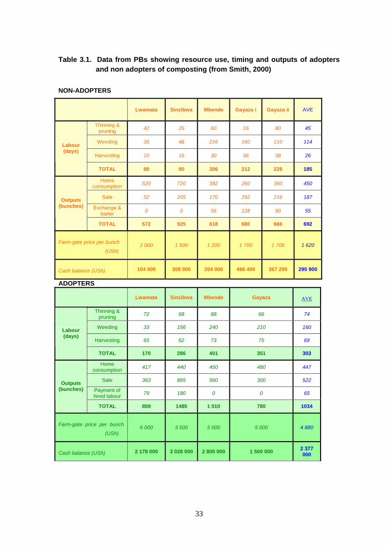
Table 3.1. Data from PBs showing resource use, timing and outputs of adopters and non adopters of composting (from Smith, 2000)

NON-ADOPTERS

Lwamata Sinzibwa Mbende Gayaza i Gayaza ii AVE

Thinning & pruning 42 26 60 16 80 45

Weeding 36 48 216 160 110 114

Harvesting 10 16 30 36 38 26

Labour (days)

TOTAL 88 90 306 212 228 185

Home consumption 520 720 392 260 360 450

Sale 52 205 170 292 216 187

Exchange & barter 0 0 56 128 90 55

Outputs (bunches)

TOTAL 572 925 618 680 666 692

Farm-gate price per bunch

(USh) 2 000 1 500 1 200 1 700 1 700 1 620

Cash balance (USh) 104 000 308 000 204 000 496 400 367 200 295 900

ADOPTERS

Lwamata Sinzibwa Mbende Gayaza AVE

Thinning & pruning 72 68 88 66 74

Weeding 33 156 240 210 160

Harvesting 65 62 73 75 69

Labour (days)

TOTAL 170 286 401 351 303

Home consumption 417 440 450 480 447

Sale 363 865 560 300 522

Payment of hired labour 79 180 0 0 65

Outputs (bunches)

TOTAL 859 1485 1 010 780 1034

Farm-gate price per bunch

(USh) 6 000 3 500 5 000 5 000 4 880

Cash balance (USh) 2 178 000 3 028 000 2 800 000 1 500 000 2 377 000

33

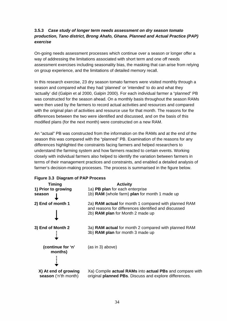
3.5.3 Case study of longer term needs assessment on dry season tomato production, Tano district, Brong Ahafo, Ghana. Planned and Actual Practice (PAP) exercise On-going needs assessment processes which continue over a season or longer offer a way of addressing the limitations associated with short term and one off needs assessment exercises including seasonality bias, the masking that can arise from relying on group experience, and the limitations of detailed memory recall. In this research exercise, 23 dry season tomato farmers were visited monthly through a season and compared what they had ‘planned’ or ‘intended’ to do and what they ‘actually’ did (Galpin et al 2000, Galpin 2000). For each individual farmer a “planned” PB was constructed for the season ahead. On a monthly basis throughout the season RAMs were then used by the farmers to record actual activities and resources and compared with the original plan of activities and resource use for that month. The reasons for the differences between the two were identified and discussed, and on the basis of this modified plans (for the next month) were constructed on a new RAM. An “actual” PB was constructed from the information on the RAMs and at the end of the season this was compared with the “planned” PB. Examination of the reasons for any differences highlighted the constraints facing farmers and helped researchers to understand the farming system and how farmers reacted to certain events. Working closely with individual farmers also helped to identify the variation between farmers in terms of their management practices and constraints, and enabled a detailed analysis of farmer’s decision-making processes. The process is summarised in the figure below.

Figure 3.3 Diagram of PAP Process Timing Activity 1) Prior to growing season

1a) PB plan for each enterprise 1b) RAM (whole farm) plan for month 1 made up

2) End of month 1 2a) RAM actual for month 1 compared with planned RAM and reasons for differences identified and discussed 2b) RAM plan for Month 2 made up

3) End of Month 2

3a) RAM actual for month 2 compared with planned RAM 3b) RAM plan for month 3 made up

(continue for ‘n’

months)

(as in 3) above)

X) At end of growing season (‘n’th month)

Xa) Compile actual RAMs into actual PBs and compare with original planned PBs. Discuss and explore differences.

34

Several important points emerged form the exercise including: • The impact of social obligations on labour availability e.g. farmers were surprised

by the time spent at funerals and consequent delays to operations • Farmers use very high rates of chemicals, often using more than one with the

same active ingredient. They demonstrated poor knowledge of chemicals and lacked access to good information.

• The highly volatile nature of the tomato market and the consequent dramatic impact of downturns on resource use, activities and returns.

• The vulnerability of the enterprise to the continuing health of the farmer e.g. illness for one week could result in no irrigation of the crop.

An alternative approach is to use a PB to for planning the season and construct another PB on which actual practices are recorded without the use of a RAM. 3.5.4 Case study of assessing the suitability of potential innovations: Green manuring for improved soil fertility, Brong Ahafo, Ghana

This case study investigated the suitability of green manuring as a technology for use in the wet season production of vegetables in Wenchi Distric (Dorward, Galpin and Shepherd, 2003). The investigation involved in-depth studies with farmers from two villages in the District, over a period of 4 days in each village. Farmers’ current cultivation practices and problems were examined, and the alternative strategies for the introduction of green manuring to benefit wet season vegetable production explored, together with the potential impact of these strategies on the wider system.

Two main methods were used. SCDs helped to identify specific constraints to tomato production and the relative importance of soil fertility as a problem to farmers. PBs were used to identify possible strategies of including green manure into the system and to investigate the likely resource implications of these strategies. The methods were used with approximately 50 farmers of mixed literacy abilities. Initial work with the SCDs identified different systems of tomato production. These included: farmers who planted prior to the rains and hand irrigated (early irrigators) to market produce earlier and at a better price; farmers who planted on mounds with the rains and intercropped; farmers who planted on ridges with the rains; and farmers who planted on the flat with the rains. In each of the two villages SCDs were developed, and scored by representative farmers for each of the systems. The scoring indicated important differences in the priorities of ‘early irrigators’ and those that plant with the rains. Those planting with the rains scored marketing problems higher as they are selling during the peak of production. ‘Early irrigators’ scored production problems higher they as they are producing when supplies are low and prices high and therefore consider low yields and some of its causes to be more important. These findings were similar for both villages but soil fertility was of much greater importance in one due to the high population resulting in land scarcity and over use.

35

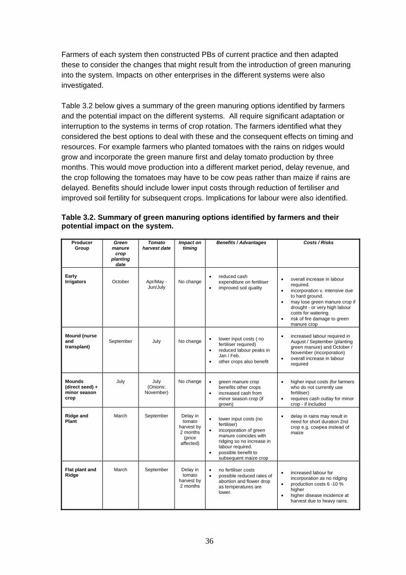
Farmers of each system then constructed PBs of current practice and then adapted these to consider the changes that might result from the introduction of green manuring into the system. Impacts on other enterprises in the different systems were also investigated. Table 3.2 below gives a summary of the green manuring options identified by farmers and the potential impact on the different systems. All require significant adaptation or interruption to the systems in terms of crop rotation. The farmers identified what they considered the best options to deal with these and the consequent effects on timing and resources. For example farmers who planted tomatoes with the rains on ridges would grow and incorporate the green manure first and delay tomato production by three months. This would move production into a different market period, delay revenue, and the crop following the tomatoes may have to be cow peas rather than maize if rains are delayed. Benefits should include lower input costs through reduction of fertiliser and improved soil fertility for subsequent crops. Implications for labour were also identified. Table 3.2. Summary of green manuring options identified by farmers and their potential impact on the system.

Producer Group

Green manure

crop planting

date

Tomato harvest date

Impact on timing

Benefits / Advantages Costs / Risks

Early Irrigators

October

Apr/May - Jun/July

No change

• reduced cash

expenditure on fertiliser • improved soil quality

• overall increase in labour required.

• incorporation v. intensive due to hard ground.

• may lose green manure crop if drought - or very high labour costs for watering.

• risk of fire damage to green manure crop

Mound (nurse and transplant)

September

July

No change

• lower input costs ( no fertiliser required)

• reduced labour peaks in Jan / Feb.

• other crops also benefit

• increased labour required in

August / September (planting green manure) and October / November (incorporation)

• overall increase in labour required

Mounds (direct seed) + minor season crop

July

July

(Onions: November)

No change

• green manure crop

benefits other crops • increased cash from

minor season crop (if grown)

• higher input costs (for farmers

who do not currently use fertiliser)

• requires cash outlay for minor crop - if included

Ridge and Plant

March

September

Delay in tomato

harvest by 2 months

(price affected)

• lower input costs (no fertiliser)

• incorporation of green manure coincides with ridging so no increase in labour required.

• possible benefit to subsequent maize crop

• delay in rains may result in

need for short duration 2nd crop e.g. cowpea instead of maize

Flat plant and Ridge

March

September

Delay in tomato

harvest by 2 months

• no fertiliser costs • possible reduced rates of

abortion and flower drop as temperatures are lower.

• increased labour for incorporation as no ridging

• production costs 6 -10 % higher

• higher disease incidence at harvest due to heavy rains.

36

Suitability assessment can therefore improve the research process by working with farmers to explore systems and resource implications in order to identify options for new systems, establish whether they are worth pursuing and what then to focus on in subsequent trials. Suitability assessment is by design a site specific investigation of particular circumstances. Time and cost limitations are likely to mean that such exercises can not be widely replicated. However wider verification could be achieved by undertaking brief formal surveys or semi structured interviews to explore the extent to which the findings apply more widely. In the above example the focus of such a survey would be to identify wet season tomato categories, production methods and the importance of soil fertility as a constraint to farmers. 3.5.5 Case studies of the use of PFM methods in on farm research in Ghana and Kenya 3.5.5.1 Ghana – recording and monitoring The suitability assessment described above for wet season tomato production was conducted with a view to developing on farm trials. Due to funding constraints the trials to investigate the key issues identified above ie for each system of tomato production, the timing of green manure and the impact on the productivity and timing of subsequent crops, were not implemented. However, the positive experience of using PFM methods with farmers led to the decision to use them for recording activities on the ongoing dry season green manuring trials. A system of recording and monitoring that was easy for farmers to use was developed with farmers as indicated in the figure below. Figure 3.4 Example layout of recording grids

Plot 1 WK1 WK2 WK3 WK4 Activities

Inputs

Yield

Fruit Quality

Plot 2 WK1 WK2 WK3 WK4

Activities

Inputs

Yield

Fruit Quality

37

Photograph 3.1 Farmer completing a recording grid for the monitoring of on farm trials

The record system was based on simple recording grids. The design of the layout, content of the record, and the symbols were made by the farmers, in collaboration with the extension workers / researchers. This was initially constructed interactively on the ground and then transferred to large (A1) flip-chart size sheets of paper. For each month the recording grids were drawn onto the A1 sheet by the extension worker and were then filled in by the farmers. The position of the plots on the paper reflected their relative positions in the field. Visits were undertaken at the end of each month to discuss the recorded data and events of the past month and clarify any points as necessary. During these visits the researcher / extension worker also discussed next month’s activities and, together with the farmer, drew up the recording grid for the next month. Regular visits of more than once a month proved to be essential in the early stages when some farmers, particularly the less literate ones, needed help with the recording system. The diagrams below are examples of the recording grid system used for the harvesting period. Criteria included were: yield (quantity), size of fruit, and quality of fruit. The symbols used were identified by the farmers and are given below.

38

Figure 3.5 Examples of records for participatory research

3.5.5.2 Kenya – planning, recording and monitoring Two farmer groups planned the next seasons’ on farm trials investigating a novel ‘push-pull’ system of food and forage production in the Central Kenyan Highlands. The ‘push-pull’ system is an Integrated Pest Management approach that involves growing Desmodium amongst maize, surrounded by a perimeter of Napier grass. The Desmodium ‘pushes’ stem borer moths away from the crop whilst the Napier grass attracts ie ‘pulls’ the moths to the perimeter. This system aims to reduce maize losses from stem borer and to increase the production of maize, and of forage for smallholder dairy cattle. Research staff and the farmer groups used PBs to plan activities, inputs, outputs, timing and what was needed to record them for both the ‘push-pull’ and ‘control’ maize only plots. The farmers then recorded these and at regular meetings with research staff who summarised the information on to PBs on flip charts.

39

The experience in Ghana and Kenya confirmed the importance of PFM methods for developing a common framework for research and farmers to articulate and agree the focus of the research, how the research is to be carried out and how it is evaluated. For example the process allowed farmers of different levels of literacy to participate fully in the whole research activity. Furthermore the discussion enabled participants to agree appropriate and understandable visual means of recording units and measurements eg different coin sizes could be used to represent tomato fruit sizes harvested in the Ghana research. Response from farmers indicated that overall the advantages of PFM methods in these activities included providing: • Easier recording methods for non and semi-literate farmers • Helping in communication between literate and non-literate farmers • Easier methods of analysis compared with written records for all farmers 3.5.5.3 Case studies of the use of PFM methods in extension in Zimbabwe and Ghana As part of a project to explore the use of PFM methods in extension, extension workers from two Districts in Zimbabwe were trained in their use and asked to use the methods in their own wards over a seven month period (Dorward, 1999). A feedback workshop and other activities were used to evaluate the methods. Uses of PBs by extension staff working with farmers included planning new enterprises (e.g. broiler poultry production) comparing enterprises (e.g. rabbit vs poultry production) or considering modifications to existing enterprises (e.g. use of locally available inputs vs external inputs for maize production). Overall feedback from both farmers and extension workers was positive and PBs had been useful for jointly exploring management options. A research project used PBs over two production periods with poultry broiler producers in the Accra area of Ghana. One of the objectives of the research was to explore the use of PBs as an extension tool. Extension workers were trained in the use of PBs and worked with groups of broiler producers. Generally farmers and extension workers reported that the process had been beneficial particularly in terms of: assessing capital requirements; identification of costs, prices and timing of sales to achieve profitable production; overall planning and scheduling eg for activities such as vaccination. 3.6 Scaling up The use of PFM in this document has generally been in the context of either ‘research’ eg for needs assessment, understanding farmer resource use, or ‘development’ eg by advisors to assist individual or groups of farmers with planning. The latter is about

40

specific situations in terms of farmers and groups whilst the former can be used in multiple sites and potentially the information can be put together in such a way as to enable generalisable understanding and the presentation of conclusions. Here, there are particular considerations concerning a) how information from PFM methods can be ‘added together’ and b) how in general data is collected and analysed to enable reliable generalisations to be made. Care needs to be taken however not to collect data simply for the sake of it: clear reasons for data collection are needed and realistic benefis identified otherwise there is a danger of repeating mistakes made in the 1980s when large amounts of farmer, extension and researchers’ time was spent collecting data that was not allways analysed and that was often of little or no direct or indirect use to farmers. Examples of combining findings from SCDs include work in Bangladesh by Gaunt et al (2003), which amongst other things examined farmers’ perceptions of problems in rice cultivation. In this work the authors were able to assess the extent of the problems identified in SCDs constructed with five groups of farmers by counting the number references to particular problems and summarising them in a single table. Commonalities could be relatively easily identified given the small number SCDs but would be more difficult to do meaningfully with large numbers. In this case a more rigorous means of how to achieve valid combinations has been explored by Burn (2000). Burn (2000) identified two difficulties in combining SCDs. The first concerns the interaction of multiple causes i.e. when a problem has two or more causes these causes may not act independently of one another. Secondly, that no account is taken of the difference between importance and probability of occurrence when scoring. Burns (2000) uses Bayesian Belief Networks BBNs) to reformulate SCDs which overcomes these two difficulties and allows several diagrams to be combined meaningfully. Essentially Burn’s approach is to construct a ‘pooled’ causal diagram which allows a summary of the individual SCDs and the ‘distance’ between the individual SCDs and the ‘pool’ to be measured. Particular groups that are very different from the ‘norm’ can be identified and assessed to provide understanding of their different perceptions. Burn (2000) makes an analogy with the conventional statistical practice of fitting a regression model to a set of data points and examining the data points which are markedly different from the expected data values as predicted by the model. The use of BBNs do provide a rational way of attempting to combine or pool the results of several SCDs but they require specific statistical expertise, and it is necessary to obtain probabilities of causes from participants. Results from several Participatory Budgets can be combined using a database (e.g. Microsoft Access), or the ‘pivot table’ function in Microsoft Excel, which acts as a simplified database. Resources and activities need to be labelled and coded in the database. Relationships (regression and correlation functions) between different resources, and ‘average’ figures for all the budgets, together with other statistical functions (e.g. standard deviation etc.) can then be calculated. An example of the type of results possible from this analysis is given below.

41

A spreadsheet was used to analyse the results from PBs constructed to assess planned and actual activities of 23 tomato producers in Brong Ahafo, Ghana. Comparisons between farmers were made and overall patterns identified. Two examples of the type of analysis that is possible using a spreadsheet are given below.

The Figure above compares planned income and actual income plotted against field size. The graph shows that actual income was generally lower than planned income which was mainly due to marketing problems experienced that year. The graph also indicates that income did not rise with increases in field size because income was limited by how much farmers could sell rather than how much they produced. Planned and actual labour figures over the season are given in Figure 3.7 below. The graph shows that from mid-November, planned labour demand was generally higher than actual labour used. The overall pattern of labour demand over the season is also demonstrated.

Figure 3.6 Scattergraph of Planned Income (INCP) and Actual Income

(INCA) by

(Sept.)

Figure 3.7 Graph showing average man-days labour per week

0

2

4

6

8

10

12

1.1 1.2 1.3 1.4 2.1 2.2 2.3 2.4 3.1 3.2 3.3 3.4 4.1 4.2 4.3 4.4 5.1 5.2 5.3 5.4 6.1 6.2 6.3 6.4 7.1 7.2 7.3 7.4

Weeks (Sept. to March)

Man-days /week

Av. mandays / week (actual) Av. mandays / week (planned)

field size

2000000

3000000

4000000

5000000

6000000

7000000

8000000

Income (cedis)

0

1000000

0 0.5 1 1.5 2 2.5 3 3.5 4

Field size (acres)

INCP INCA Linear (INCP) Linear (INCA)

42

Any quantitative information contained in PBs can be combined and analysed e.g. amounts or costs of specific inputs or outputs. The process highlighted several differences which occurred between the farmers planned and actual activities and resource use (many of these observations did not require the level of analysis described above) e.g. • Some disruption of planned activities occurred. Time spent at funerals was a main

cause of delays in the implementation of planned activities. This was particularly important for heads of families.

• Unexpected rains reduced the labour required for watering. • The activity of ‘shading’ was an additional activity due to the higher than expected

temperatures. • Actual inputs varied from those planned, due to availability of inputs but also due to

farmers responding to the condition of the crop etc. Prices of inputs were generally as expected.

• The harvest yield was severely reduced, primarily due to the very low prices and the lack of buyers. This was attributed to the fact that there were too many tomatoes on the market.

• The poor market and prices also had an impact on labour at harvest, resulting in average planned labour being higher than average actual labour.

• Actual income was much lower than predicted income due to problems of marketing of produce.

A more straightforward approach could be to present an ‘average PB’ made up of combined results from several PBs with average figures for labour and different inputs etc. given. In the comparison of adopters and non adopters of composting for plantain banana production in Uganda referred to earlier, Smith (2000) demonstrated that PBs can be combined to analyse differences in resource use and production. Working with groups of farmers from five villages in central Uganda, PBs generated with farmers using composting were combined and compared with PBs for farmers not using composting. The sample size was too small to be statistically viable but the results indicated clear differences of resource use, particularly labour, and output levels. As indicated in table 3.1 above, labour use, inputs, banana yield, price and cash income were all higher in the system using composting. Figure 3.8 below illustrates differences in monthly cash income between adopters and non adopters derived from the combined PBs.

43

Figure 3.8 Monthly cash income per acre for adopters and non adopters of composting (Smith, 2000)

0

50000

100000

150000

200000

250000

300000

350000

400000

Jan Feb Mar Apr May Jun Jul Aug Sept Oct Nov Dec

Cas

h in

com

e (U

sh /

acre

)

Adopters Non-adopters

If this approach is used some indication of the variation between farmers should be given e.g. minimum and maximum, or standard deviation values. As the above examples remind us, PFM methods can produce numerical data. However if these numbers are combined to produce information from which general conclusions can be drawn e.g.for policy, then statistical principles must apply (as illustrated in the work by Burn noted earlier). In general these include issues of representativeness and sampling, standardisation of data collection tools and comparability of data. How this can be achieved using participatory tools has been explored and developed by Barahona and Levy (2002) and examples include work in India (PRAXIS, 2001), Colombia (Moser and Mcllwaine, 2000) and Malawi (Levy, 2003). This raises concerns about empowerment and ethical issues and whether “…the fundamental principles of participation [are] undermined by the modifications that we need to make if we are to generate data for use beyond the local level” (Barahona and Levy, 2002). The experience and benefits of using ‘participatory numbers’ are explored further in Chambers (2003). 3.7 Conclusions The motivation to identify and develop PFM methods was essentially based on the idea that smallholder farmers in CDR systems could improve their decision making through the application of farm management type tools, provided these were developed with the farmers in the context of their socioeconomic and agroecological conditions. As indicated above such tools can be used directly by farmers to help them in their decision making. They are also useful for advisors and researchers both as a means of advising farmers

44

and as a means of learning from and with farmers about the constraints they face and the reasons for the choices they make. As with PLA approaches, central to the use of Participatory Farm Management methods is the understanding that the farmer is the decision-maker and that he or she takes the risks associated with change, not the advisor or researcher. PFM methods are seen therefore as useful tools to assist the farmer in his or her decision-making process, rather than techniques to help persuade farmers to adopt practices advocated by others, or simply to elicit information. The positive benefits of the use of PFM observed by the authors and others has been achieved by striving to create a mutual learning environment between facilitator and farmer, even where data collection has been an objective. This, as with any participatory methodology, is highly dependent on the attitude and skills of the facilitator. PFM methods may be taught in a classroom but they will only be understood in their application in the field, and only then if the facilitator is not driven by the method but recognises the need for flexibility and openness in learning with farmers. These methods are not blueprints but should be developed and modified as circumstances require and in this spirit the authors welcome feedback on their use and development. For further information contact Peter Dorward – p.t.dorward@reading.ac.uk or Derek Shepherd - d.d.shepherd@reading.ac.uk School of Agriculture, Policy and Development University of Reading Box 236 Reading RG6 6AT UK References Barahona, C. and Levy, S. (2002). How to Generate Statistics and Influence Policy Using Participatory Methods in Research. Statistical Service Centre, University of Reading Working Paper (www. reading.ac.uk/~snsbarah/sscwp). Burn, R.W. (2000). Quantifying and Combining Causal Diagrams. Statistical Services Centre. The University of Reading. Carruthers, I. and Chambers, R. (1981) Rapid Apraisal for Rural Development. Agricultural Administration 8, (6), 407-422. Chambers, R. (1991) PRA Methods for Quantifying and Ranking. IDS, University of Sussex (mimeo). Chambers, R. (1993). Challenging the Professions. Frontiers for Rural Development. IT Publications, London.

45

Chambers, R. (1996). Relaxed and participatory appraisal notes on practical approaches and methods. Rural Systems Research and Farming Systems Research Projects. University of Khon Kaen, Thailand. Chambers, R. (1997). Whose Reality Counts? Putting the last first. Intermediate Technology Publications, London. Chambers, R. (2003). Participation and Numbers. PLA Notes, 47, 6-12. Cornwall, A., Guijt, I. and Welbourne, A. (1994). Acknowledging processes: challenges for agricultural research and extension methodology. In Beyond Farmer First. Rural peoples’ knowledge, agricultural research and extension practice. (Eds I. Scoones, J. Thompson). Intermediate Technology Publications, London. Dorward, P. (1999). Participatory Farm Management Methods for Improved Agricultural Extension with Smallholder Farmers in Zimbabwe. PhD thesis. The University of Reading. Dorward, P., Galpin, M. and Shepherd, D.D. (2003).. A Case Study on Green Manuring Options for Tomato Producers in Ghana. Agricultural Systems, 75, 97-117. Dorward, P., Shepherd, D.D., and Woolmer, W. (1997). Developing farm management type methods for participatory needs assessment. Agricultural Systems 55 (2), 239-256. Galpin, M. (2000). The Development and Evaluation of Participatory Farm Management Methods for Research Needs Assessment with Smallholder Farmers. PhD thesis, The University of Reading. Galpin, M, Dorward, P. and Shepherd D.D. (2000). Participatory Farm Management Methods for Agricultural Research and Extension: A Training Manual. The University of Reading and DFID. Gaunt, J., White, S.K., Best, J.R., Sutherland, A.J., Norrish, P., Robinson, E.J.Z., Zahid Huossain and Palmer-Jones, R.J. (2003). The Researcher-Farmer Interface in the Rice-Wheat System: Moving From Agricultural Productivity to Livelihoods. In Improving the Productivity and Sustainability of Rice-Wheat Systems: Issues and Impacts. ASA Special Publication 65. Madison, USA. Harding, T.J. (1982). Farm management advice to peasant agriculture: the transfer of technology. Journal of Agricultural Economics 33, 47-56. Levy, S. (2003). Are We Targeting the Poor? Lessons from Malawi. PLA Notes, 47, 19-24.

46

Lightfoot, C., Dalsgaard, J. P. and Bimbao, M.A. (1993). Farmer Participatory Procedures for Managang and Monitoring Sustainable Farming Systems. Journal of the Asian Farming Systems Association, 2:1, 66-87. Lightfoot, C., De Guia, O. Jr., Aliman, A., and Ocado, F. (1989). Systems Diagrams to Help Farmers Decide in On Farm Research. In Farmer First: Farmer Innovation and Agricultural Research. PP 93-105 (Eds R. Chambers, A.Pacey and L. Thrupp). IT Publications, London. Mascarenhas, J. , Shah, P., Joseph, S., Jayakaran, R., Devavaran, J., Ramachandran, V., Fernandez, A., Chambers, R., and Pretty, J. (Eds) (1991). Preceedings of the Bangalor PRA Workshop, February 1991. RRA Notes, 13. Moser, C. and Mcllwaine, C. (2000). Urban Poor Perceptions of Violence and Exclusion in Colombia. Latin American and Caribbean Region, Environmentally and Socially Sustainable Development Sector Management Unit, Washington DC: World Bank. PRAXIS (2001). The Politics of Poverty: A Tale of the Living Dead in Bolangir. Books for Change, SKIP House, Bangalor. Pretty, J. N., Guijt, I., Thompson, J. and Scoones, I. (1995). A trainers Guide for Participatory Learning and Action. IIED Participatory Methododlogy Series. IIED, London. Rehman, T. and Dorward, A. (1984). Farm Management techniques and their relevance to administration, research and extension in agricultural development: Part 1 - Their evolution and use in developed countries; Part 2 - An appraisal of their potential in LDCs. Agricultural Administration 15, 177-190, 239-254. Scoones, I. and Thompson, J. (1994). Beyond farmer first: rural peoples’ knowledge, agricultural research and extension practice. Intermediate Technology Publications. Shaner, W. W., Phillip, P. F. and Schmehl, W.R. (1982) Farming Systems Research and Development – Guidelines for developing Countries. Westview Press, Boulder, Colorado. Smith, K.V. (2000). Factors Affecting Adoption of Introduced Innovations: Use of Composting in Plantain Production by Smallholder Farmers in Uganda. MSc thesis. The University of Reading.

47