partial differential equations notes
DESCRIPTION
PDE notes as taught in the course MTH203 in IIT Kanpur (by T Muthukumar)TRANSCRIPT

Mathematics-IIIMTH-203
I Semester, 2011-12
Contents
Contents1 Lecture-23 2
1.1 Eigenvalue Problem . . . . . . . . . . . . . . . . . . . . . . . . . . . . . . . . . . . . . . . . . 21.2 Sturm-Liouville Problem . . . . . . . . . . . . . . . . . . . . . . . . . . . . . . . . . . . . . . . 41.3 Orthogonality . . . . . . . . . . . . . . . . . . . . . . . . . . . . . . . . . . . . . . . . . . . . . 51.4 Singular Problems . . . . . . . . . . . . . . . . . . . . . . . . . . . . . . . . . . . . . . . . . . 6
2 Lecture-24 72.1 Periodic Functions . . . . . . . . . . . . . . . . . . . . . . . . . . . . . . . . . . . . . . . . . . 72.2 Fourier Series . . . . . . . . . . . . . . . . . . . . . . . . . . . . . . . . . . . . . . . . . . . . . 82.3 Piecewise Smooth . . . . . . . . . . . . . . . . . . . . . . . . . . . . . . . . . . . . . . . . . . . 10
3 Lecture-25 113.1 Orthogonality . . . . . . . . . . . . . . . . . . . . . . . . . . . . . . . . . . . . . . . . . . . . . 113.2 Odd-Even Functions . . . . . . . . . . . . . . . . . . . . . . . . . . . . . . . . . . . . . . . . . 123.3 Fourier Sine-Cosine Series . . . . . . . . . . . . . . . . . . . . . . . . . . . . . . . . . . . . . . 123.4 Fourier Integral . . . . . . . . . . . . . . . . . . . . . . . . . . . . . . . . . . . . . . . . . . . . 13
4 Lecture-26 144.1 PDE-Introduction . . . . . . . . . . . . . . . . . . . . . . . . . . . . . . . . . . . . . . . . . . 144.2 Gradient and Hessian . . . . . . . . . . . . . . . . . . . . . . . . . . . . . . . . . . . . . . . . 144.3 PDE . . . . . . . . . . . . . . . . . . . . . . . . . . . . . . . . . . . . . . . . . . . . . . . . . . 154.4 Types of PDE . . . . . . . . . . . . . . . . . . . . . . . . . . . . . . . . . . . . . . . . . . . . . 154.5 PDE-Solution . . . . . . . . . . . . . . . . . . . . . . . . . . . . . . . . . . . . . . . . . . . . . 164.6 Well Posedness . . . . . . . . . . . . . . . . . . . . . . . . . . . . . . . . . . . . . . . . . . . . 16
5 Lecture - 27 175.1 First order PDE . . . . . . . . . . . . . . . . . . . . . . . . . . . . . . . . . . . . . . . . . . . 175.2 Solving First Order PDE . . . . . . . . . . . . . . . . . . . . . . . . . . . . . . . . . . . . . . 17
6 Lecture - 28 186.1 Transport Equation . . . . . . . . . . . . . . . . . . . . . . . . . . . . . . . . . . . . . . . . . 186.2 Cauchy Problem . . . . . . . . . . . . . . . . . . . . . . . . . . . . . . . . . . . . . . . . . . . 19
1
7 Lecture - 29 217.1 Second Order PDE . . . . . . . . . . . . . . . . . . . . . . . . . . . . . . . . . . . . . . . . . . 217.2 Classification . . . . . . . . . . . . . . . . . . . . . . . . . . . . . . . . . . . . . . . . . . . . . 217.3 Standard Forms . . . . . . . . . . . . . . . . . . . . . . . . . . . . . . . . . . . . . . . . . . . . 23
8 Lecture - 30 248.1 Three Basic Linear PDE . . . . . . . . . . . . . . . . . . . . . . . . . . . . . . . . . . . . . . . 248.2 Laplace Equation . . . . . . . . . . . . . . . . . . . . . . . . . . . . . . . . . . . . . . . . . . . 25
9 Lecture - 31 259.1 Dirichlet Problem . . . . . . . . . . . . . . . . . . . . . . . . . . . . . . . . . . . . . . . . . . . 259.2 DP On Rectangle . . . . . . . . . . . . . . . . . . . . . . . . . . . . . . . . . . . . . . . . . . . 25
10 Lecture - 32 2810.1 Laplace Equation . . . . . . . . . . . . . . . . . . . . . . . . . . . . . . . . . . . . . . . . . . . 2810.2 Laplacian on a 2D-Disk . . . . . . . . . . . . . . . . . . . . . . . . . . . . . . . . . . . . . . . 28
11 Lecture - 33 3011.1 Laplace Equation . . . . . . . . . . . . . . . . . . . . . . . . . . . . . . . . . . . . . . . . . . . 3011.2 Laplacian on a 3D-Sphere . . . . . . . . . . . . . . . . . . . . . . . . . . . . . . . . . . . . . . 31
12 Lecture-34 3312.1 Eigenvalues of Laplacian . . . . . . . . . . . . . . . . . . . . . . . . . . . . . . . . . . . . . . . 3312.2 Computing Eigenvalues . . . . . . . . . . . . . . . . . . . . . . . . . . . . . . . . . . . . . . . 3312.3 In Rectangle . . . . . . . . . . . . . . . . . . . . . . . . . . . . . . . . . . . . . . . . . . . . . 3312.4 In Disk . . . . . . . . . . . . . . . . . . . . . . . . . . . . . . . . . . . . . . . . . . . . . . . . 3412.5 Bessel’s Function . . . . . . . . . . . . . . . . . . . . . . . . . . . . . . . . . . . . . . . . . . . 35
13 Lecture - 35 3613.1 1D Heat Equation . . . . . . . . . . . . . . . . . . . . . . . . . . . . . . . . . . . . . . . . . . 3613.2 Solving for Circular Wire . . . . . . . . . . . . . . . . . . . . . . . . . . . . . . . . . . . . . . 38
14 Lecture - 36 3914.1 1D Wave Equation . . . . . . . . . . . . . . . . . . . . . . . . . . . . . . . . . . . . . . . . . . 39
15 Lecture - 37 4115.1 Duhamel’s Principle . . . . . . . . . . . . . . . . . . . . . . . . . . . . . . . . . . . . . . . . . 41
16 Lecture - 38 4416.1 d’Alembert’s Formula . . . . . . . . . . . . . . . . . . . . . . . . . . . . . . . . . . . . . . . . 44
1 Lecture-231.1 Eigenvalue ProblemMotivation
• Consider the problem,y′′(x) + λy(x) = 0 x ∈ (a, b).
• For a given λ ∈ R, we know the general solution, depending on whether λ < 0, λ = 0 or λ > 0.
• What if λ is unknown too?
• Note that y ≡ 0 is a trivial solution, for all λ ∈ R.
2

Eigenvalue problem
Definition 1.1. For a differential operator L, we say
Ly(x) = λy(x)
to be the eigenvalue problem (EVP) corresponding to the differential operator L, where both λ and y areunknown.
In an EVP we need to find all λ ∈ R for which the given ODE (equation) is solvable.Does EVP ring any bell? Any similarity with diagonalisation of matrices from Linear Algebra? Think
about it!
Eigenvalues and Eigen FunctionsExample 1.1. For instance, if L = −d2
dx2 then its corresponding eigenvalue problem is
−y′′ = λy.
Definition 1.2. A λ ∈ R, for which the EVP corresponding to L admits a non-trivial solution yλ is calledan eigenvalue of the operator L and yλ is said to be an eigen function corresponding to λ.
Explicit Computation
• Consider the boundary value problem,y′′ + λy = 0 x ∈ (0, a)
y(0) = y(a) = 0.
• This is a second order ODE with constant coeffcients.
• Its characteristic equation is m2 + λ = 0.
• Solving for m, we get m = ±√−λ.
• Note that the λ can be either zero, positive or negative.
• If λ = 0, then y′′ = 0 and the general solution is y(x) = αx+ β, for some constants α and β.
• Since y(0) = y(a) = 0 and a 6= 0, we get α = β = 0. Thus, we have no non-trivial solution correspondingto λ = 0.
λ < 0, Negative
• If λ < 0, then ω = −λ > 0.
• Hence y(x) = αe√ωx + βe−
√ωx.
• Using the boundary condition y(0) = y(a) = 0, we get α = β = 0 and hence we have no non-trivialsolution corresponding to negative λ’s.
3
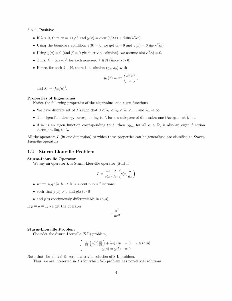
λ > 0, Positive
• If λ > 0, then m = ±i√λ and y(x) = α cos(
√λx) + β sin(
√λx).
• Using the boundary condition y(0) = 0, we get α = 0 and y(x) = β sin(√λx).
• Using y(a) = 0 (and β = 0 yields trivial solution), we assume sin(√λa) = 0.
• Thus, λ = (kπ/a)2 for each non-zero k ∈ N (since λ > 0).
• Hence, for each k ∈ N, there is a solution (yk, λk) with
yk(x) = sin(kπx
a
),
and λk = (kπ/a)2.
Properties of EigenvaluesNotice the following properties of the eigenvalues and eigen functions.
• We have discrete set of λ’s such that 0 < λ1 < λ2 < λ3 < . . . and λn →∞.
• The eigen functions yλ corresponding to λ form a subspace of dimension one (Assignment!), i.e.,
• if yλ is an eigen function corresponding to λ, then αyλ, for all α ∈ R, is also an eigen functioncorresponding to λ.
All the operators L (in one dimension) to which these properties can be generalised are classified as Sturm-Liouville operators.
1.2 Sturm-Liouville ProblemSturm-Liouville Operator
We say an operator L is Sturm-Liouville operator (S-L) if
L = −1q(x)
d
dx
(p(x) d
dx
)• where p, q : [a, b]→ R is a continuous functions
• such that p(x) > 0 and q(x) > 0
• and p is continuously differentiable in (a, b).
If p ≡ q ≡ 1, we get the operator
− d2
dx2 .
Sturm-Liouville ProblemConsider the Sturm-Liouville (S-L) problem,
ddx
(p(x) dydx
)+ λq(x)y = 0 x ∈ (a, b)
y(a) = y(b) = 0.
Note that, for all λ ∈ R, zero is a trivial solution of S-L problem.Thus, we are interested in λ’s for which S-L problem has non-trivial solutions.
4

Solution Space and Eigen Space
• Let V0 be the real vector space of all y : [a, b]→ R such that y(a) = y(b) = 0.
• If λ is an eigenvalue for S-L operator, we define the subspace of V0 as
Wλ = y ∈ V0 | y solves S-L problem.
Existence
Theorem 1.3. Under the hypotheses on p and q, there exists an increasing sequence of eigenvalues
• 0 < λ1 < λ2 < λ3 < . . . < λn < . . . with λn →∞
• and Wn = Wλnis one-dimensional.
• Conversely, any solution y of the S-L problem is in Wn, for some n.
1.3 OrthogonalityInner Product
We define the following inner product in the solution space V0,
〈f, g〉 :=∫ b
a
q(x)f(x)g(x) dx.
Definition 1.4. We say two functions f and g are perpendicular or orthogonal with weight q
• if 〈f, g〉 = 0.
• we say f is of unit length if its norm ‖f‖ =√〈f, f〉 = 1.
Orthogonality of Eigenfunctions
Theorem 1.5. With respect to the inner product defined above in V0, the eigen functions corresponding todistinct eigenvalues of the S-L problem are orthogonal.
Proof
Proof. Let yi and yj are eigen functions corresponding to distinct eigenvalues λi and λj . We need to showthat 〈yi, yj〉 = 0. Recall that L is the S-L operator and hence Lyk = λkyk, for k = i, j.Consider
λi〈yi, yj〉 = 〈Lyi, yj〉 =∫ b
a
qLyiyj dx
= −∫ b
a
d
dx
(p(x)dyi
dx
)yj(x) =
∫ b
a
p(x)dyidx
dyj(x)dx
dx
= −∫ b
a
yi(x) ddx
(p(x)dyj
dx
)= 〈yi, Lyj〉 = λj〈yi, yj〉.
Thus (λi − λj)〈yi, yj〉 = 0. But λi − λj 6= 0, hence 〈yi, yj〉 = 0.
5

1.4 Singular ProblemsSingular Problems
• What we have seen is the Regular S-L problems.
• It is regular because the interval under consideration (a, b) was finite and the functions p(x) and q(x)were positive and continuous on the whole interval.
• We say a problem is Singular,
– if the interval is infinite or– interval is finite, but p or q vanish at one (or both) endpoints or– interval is finite, but p or q is discontinuous at one (or both) endpoints.
Legendre Equation
• The Legendre equation(1− x2)y′′ − 2xy′ + λy = 0 for x ∈ [−1, 1].
is an example of a singular S-L problem.
• This is easily seen by rewriting the Legendre equation as
d
dx
((1− x2)dy
dx
)+ λy = 0 for x ∈ [−1, 1].
• q ≡ 1 and p(x) = 1− x2 vanish at the endpoints x = ±1.
Solving Legendre Equation
• The end points x = ±1 are regular singular point.
• The coefficients P (x) = −2x1−x2 and Q(x) = λ
1−x2 are analytic at x = 0, the origin with radius ofconvergence R = 1.
• We look for power series form of solutions y(x) =∑∞k=0 akx
k.
• a2 = −λa02 , a3 = (2−λ)a1
6 and for k ≥ 2, ak+2 = (k(k+1)−λ)ak
(k+2)(k+1) .
• y(x) = a0y1+a1y2, where y1, y2 are infinite series containing only even and odd powers of x, respectively.In particular, y1 and y2 are solutions to the Legendre equations, by choosing a0 = 1, a1 = 0 andviceversa.
Legendre Polynomial
• Note that, for k ≥ 2,ak+2 = (k(k + 1)− λ)ak
(k + 2)(k + 1) .
• Hence, for any n ≥ 2, if λ = n(n+ 1), then an+2 = 0 and hence every successive (even or odd) term iszero.
• Also, if λ = 1(1 + 1) = 2, then a3 = 0.
• If λ = 0(0 + 1) = 0, then a2 = 0.
• Thus, for each n ∈ N∪ 0, we have λn = n(n+ 1) and a polynmial Pn of degree n which is a solutionto the Legendre equation.
6
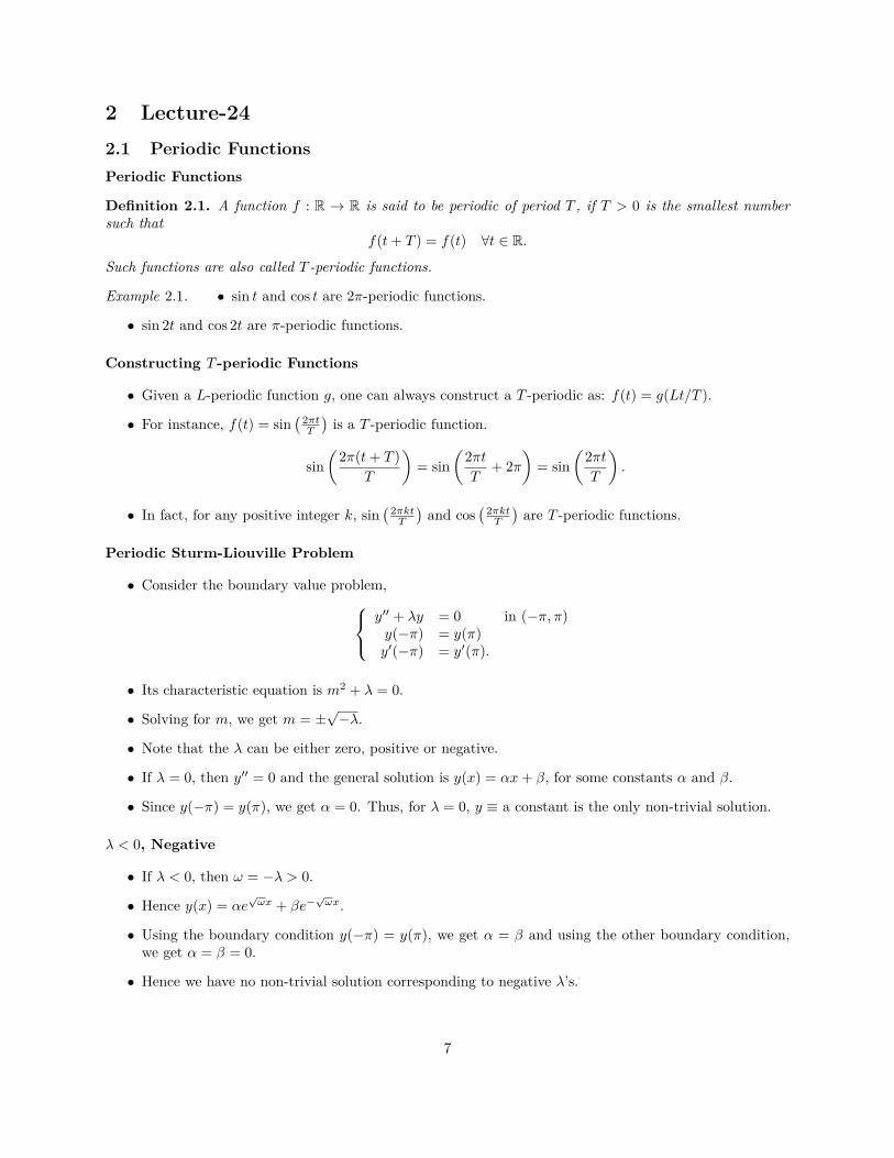
2 Lecture-242.1 Periodic FunctionsPeriodic Functions
Definition 2.1. A function f : R → R is said to be periodic of period T , if T > 0 is the smallest numbersuch that
f(t+ T ) = f(t) ∀t ∈ R.
Such functions are also called T -periodic functions.
Example 2.1. • sin t and cos t are 2π-periodic functions.
• sin 2t and cos 2t are π-periodic functions.
Constructing T -periodic Functions
• Given a L-periodic function g, one can always construct a T -periodic as: f(t) = g(Lt/T ).
• For instance, f(t) = sin( 2πtT
)is a T -periodic function.
sin(
2π(t+ T )T
)= sin
(2πtT
+ 2π)
= sin(
2πtT
).
• In fact, for any positive integer k, sin( 2πkt
T
)and cos
( 2πktT
)are T -periodic functions.
Periodic Sturm-Liouville Problem
• Consider the boundary value problem, y′′ + λy = 0 in (−π, π)y(−π) = y(π)y′(−π) = y′(π).
• Its characteristic equation is m2 + λ = 0.
• Solving for m, we get m = ±√−λ.
• Note that the λ can be either zero, positive or negative.
• If λ = 0, then y′′ = 0 and the general solution is y(x) = αx+ β, for some constants α and β.
• Since y(−π) = y(π), we get α = 0. Thus, for λ = 0, y ≡ a constant is the only non-trivial solution.
λ < 0, Negative
• If λ < 0, then ω = −λ > 0.
• Hence y(x) = αe√ωx + βe−
√ωx.
• Using the boundary condition y(−π) = y(π), we get α = β and using the other boundary condition,we get α = β = 0.
• Hence we have no non-trivial solution corresponding to negative λ’s.
7

λ > 0, Positive
• If λ > 0, then m = ±i√λ and y(x) = α cos(
√λx) + β sin(
√λx).
• Using the boundary condition, we get
α cos(−√λπ) + β sin(−
√λπ) = α cos(
√λπ) + β sin(
√λπ)
• and−α sin(−
√λπ) + β cos(−
√λπ) = −α sin(
√λπ) + β cos(
√λπ).
• Thus, β sin(√λπ) = α sin(
√λπ) = 0.
• For a non-trivial solution, we must have sin(√λπ) = 0.
• Thus, λ = k2 for each non-zero k ∈ N (since λ > 0).
• Hence, for each k ∈ N, there is a solution (yk, λk) with
yk(x) = αk cos kx+ βk sin kx,
and λk = k2 and for λ0, we have y0 = α0.
• Consider the series (eigen function expansion)
y(x) ≈∞∑k=0
akyk = a0α0 +∞∑k=1
ak (αk cos kx+ βk sin kx) .
2.2 Fourier SeriesFourier Series
Let f : R → R be a T -periodic function. We also know that, for any positive integer k, sin( 2πkt
T
)and
cos( 2πkt
T
)are T -periodic functions.
Can we find sequences ak and bk in R, and a0 ∈ R such that the infinite series
a0 +∞∑k=1
[ak cos
(2πktT
)+ bk sin
(2πktT
)]converges to f(t) for some or all t ∈ R?
Computing Fourier coefficientsTo simplify notations, let us consider a 2π-periodic function f , however, same ideas will work for a
T -periodic function. Let f be a function such that the infinite series
a0 +∞∑k=1
(ak cos kt+ bk sin kt)
converges uniformly to f . Thus,
f(t) = a0 +∞∑k=1
(ak cos kt+ bk sin kt). (1)
8

Formulae for a0, ak’s and bk’sBy integrating both sides of (1) from −π to π,∫ π
−πf(t) dt =
∫ π
−π
(a0 +
∞∑k=1
(ak cos kt+ bk sin kt))dt
= a0(2π) +∫ π
−π
( ∞∑k=1
(ak cos kt+ bk sin kt))dt
Since the series converges uniformly to f , then we can interchange integral and series. Thus,∫ π
−πf(t) dt = a0(2π) +
∞∑k=1
(∫ π
−π(ak cos kt+ bk sin kt) dt
)
But we know that ∫ π
−πsin kt dt =
∫ π
−πcos kt dt = 0, ∀k ∈ N.(Exercise!)
Hence,a0 = 1
2π
∫ π
−πf(t) dt.
To find the coefficients ak, for each fixed k, we multiply both sides of (1) by cos kt and integrate from −πto π. Consequently, we get∫ π
−πf(t) cos kt dt = a0
∫ π
−πcos kt dt
+∞∑j=1
∫ π
−π(aj cos jt cos kt+ bj sin jt cos kt) dt
=∫ π
−πak cos kt cos kt dt = πak.
Similar argument after multiplying by sin kt gives the formula for bk’s. Thus, we derived, for all k ∈ N,
ak = 1π
∫ π
−πf(t) cos kt dt
bk = 1π
∫ π
−πf(t) sin kt dt
a0 = 12π
∫ π
−πf(t) dt.
ExercisesFor any m ≥ 0 and n positive integer
• ∫ π
−πcosnt cosmtdt =
π, for m = n
0, for m 6= n.
Hence, cos kt√π
is of unit length.
9

• ∫ π
−πsinnt sinmtdt =
π, for m = n
0, for m 6= n.
Hence, sin kt√π
is of unit length.
• ∫ π
−πsinnt cosmtdt = 0.
Fourier Series and Coeffcients
Definition 2.2. For any T -periodic function f : R→ R,
• a0, ak and bk, for all k ∈ N, as defined previously are called the Fourier coefficients of f .
• Further, the infinite series
a0 +∞∑k=1
[ak cos
(2πktT
)+ bk sin
(2πktT
)], (2)
is called the Fourier series of f .
Some QuestionsGiven a 2π-periodic function f : R→ R and we know how to find the Fourier coefficients of f
• Will the Fourier series of f
a0 +∞∑k=1
(ak cos kt+ bk sin kt)
converge?
• If it converges, will it converge to f?
• If so, is the convergence point-wise or uniform etc
are questions one can ask and will not be dealt with in this course.
An AnswerAnswering our question, in all generality, is rather difficult at this stage. However, we shall answer it in
a simple version which will suffice our purposes:
Theorem 2.3. If f : R → R is a continuously differentiable (derivative f ′ exists and is continuous) T -periodic function, then the Fourier series of f converges to f(t), for every t ∈ R.
2.3 Piecewise SmoothPiecewise Smooth
Is continuity necessary for a function to admit Fourier expansion?
Definition 2.4. A function f : [a, b] → R is said to be piecewise continuously differentiable if it has acontinuous derivative f ′ in (a, b), except at finitely many points in the interval [a, b] and at each these finitepoints, the right-hand and left-hand limit for both f and f ′ exist.
10

Example
• Consider f : [−1, 1] → R defined as f(t) = |t| is continuous. It is not differentiable at 0, but it ispiecewise continuously differentiable.
• Consider the function f : [−1, 1]→ R defined as
f(t) =
−1, for − 1 < t < 0,1, for 0 < t < 1,0, for t = 0, 1,−1.
It is not continuous, but is piecewise continuous. It is also piecewise continuously differentiable.
Theorem 2.5. If f is a T -periodic piecewise continuously differentiable function,
• then the Fourier series of f converges to f(t), for every t at which f is smooth.
• At a non-smooth point t0, the Fourier series of f will converge to the average of the right and left limitsof f at t0.
3 Lecture-253.1 OrthogonalityOrthogonality
Let V be the real vector space of all 2π-periodic real valued continuous function on R.We introduce an inner product in V . For any two elements f, g ∈ V , we define:
〈f, g〉 :=∫ π
−πf(t)g(t) dt.
The inner product generalises to V the properties of scalar product in Rn (Exercise!).Recall the definition
Definition 3.1. We say two functions f and g are perpendicular or orthogonal
• if 〈f, g〉 = 0.
• we say f is of unit length if its norm ‖f‖ =√〈f, f〉 = 1.
Set, for k ∈ N,e0(t) = 1√
2π, ek(t) = cos kt√
πand fk(t) = sin kt√
π.
Example 3.1. e0, ek and fk are all of unit length. 〈e0, ek〉 = 0 and 〈e0, fk〉 = 0. Also, 〈em, en〉 = 0 and〈fm, fn〉 = 0, for m 6= n. Further, 〈em, fn〉 = 0 for all m,n.
In this new formulation, we can rewrite the formulae for the Fourier coefficients as:
a0 = 1√2π〈f, e0〉, ak = 1√
π〈f, ek〉 and bk = 1√
π〈f, fk〉.
and the Fourier series of f has the form,
f(t) = 〈f, e0〉1√2π
+ 1√π
∞∑k=1
(〈f, ek〉 cos kt+ 〈f, fk〉 sin kt) .
11
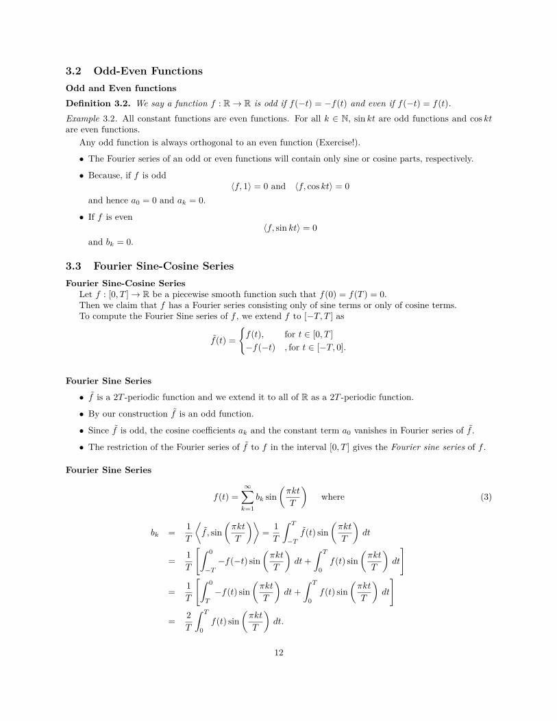
3.2 Odd-Even FunctionsOdd and Even functionsDefinition 3.2. We say a function f : R→ R is odd if f(−t) = −f(t) and even if f(−t) = f(t).Example 3.2. All constant functions are even functions. For all k ∈ N, sin kt are odd functions and cos ktare even functions.
Any odd function is always orthogonal to an even function (Exercise!).
• The Fourier series of an odd or even functions will contain only sine or cosine parts, respectively.
• Because, if f is odd〈f, 1〉 = 0 and 〈f, cos kt〉 = 0
and hence a0 = 0 and ak = 0.
• If f is even〈f, sin kt〉 = 0
and bk = 0.
3.3 Fourier Sine-Cosine SeriesFourier Sine-Cosine Series
Let f : [0, T ]→ R be a piecewise smooth function such that f(0) = f(T ) = 0.Then we claim that f has a Fourier series consisting only of sine terms or only of cosine terms.To compute the Fourier Sine series of f , we extend f to [−T, T ] as
f(t) =f(t), for t ∈ [0, T ]−f(−t) , for t ∈ [−T, 0].
Fourier Sine Series
• f is a 2T -periodic function and we extend it to all of R as a 2T -periodic function.
• By our construction f is an odd function.
• Since f is odd, the cosine coefficients ak and the constant term a0 vanishes in Fourier series of f .
• The restriction of the Fourier series of f to f in the interval [0, T ] gives the Fourier sine series of f .
Fourier Sine Series
f(t) =∞∑k=1
bk sin(πkt
T
)where (3)
bk = 1T
⟨f , sin
(πkt
T
)⟩= 1T
∫ T
−Tf(t) sin
(πkt
T
)dt
= 1T
[∫ 0
−T−f(−t) sin
(πkt
T
)dt+
∫ T
0f(t) sin
(πkt
T
)dt
]
= 1T
[∫ 0
T
−f(t) sin(πkt
T
)dt+
∫ T
0f(t) sin
(πkt
T
)dt
]
= 2T
∫ T
0f(t) sin
(πkt
T
)dt.
12

Fourier Cosine SeriesSimilarly, we could have extended f to f as,
f(t) =f(t), for t ∈ [0, T ]f(−t) , for t ∈ [−T, 0].
f is, now, an even function which can be extended as a 2T -periodic function to all of R. The Fourier seriesof f has no sine coefficients, bk = 0. The restriction of the Fourier series of f to f in the interval [0, T ] givesthe Fourier cosine series of f .
Fourier Cosine Series
f(t) = a0 +∞∑k=1
ak cos(πkt
T
)(4)
whereak = 2
T
∫ T
0f(t) cos
(πkt
T
)dt
anda0 = 1
T
∫ T
0f(t) dt.
3.4 Fourier IntegralNon-periodic functions
We know that the Fourier series of a 2π-periodic function f is given as
f(t) = a0 +∞∑k=1
(ak cos kt+ bk sin kt)
where a0, ak and bk can be computed from f .
• Can we generalise the notion of Fourier series of f , for a non-periodic function f?
• Yes! How?
• Note that the periodicity of f is captured by the integer k appearing with sin and cos.
• To generalise for non-periodic functions, we shall replace k with a real number ξ.
Fourier IntegralNote that when we replace k with ξ, the sequences ak, bk become functions of ξ and the series is replaced
with integral over R.
Definition 3.3. If f : R → R is a piecewise continuous function which vanishes outside a finite interval,then its Fourier integral is defined as
f(t) =∫ ∞
0(a(ξ) cos ξt+ b(ξ) sin ξt) dξ,
13

where
a(ξ) = 1π
∫ ∞−∞
f(t) cos ξt dt
b(ξ) = 1π
∫ ∞−∞
f(t) sin ξt dt.
4 Lecture-264.1 PDE-IntroductionPartial Derivatives
Let u : R2 → R be a two variable function,then its partial derivative (if limit exists) with respect to x isgiven as,
ux = ∂u
∂x(x, y) := lim
h→0
u(x+ h, y)− u(x, y)h
.
Similarly, one can consider partial derivative w.r.t y-variable and higher order derivatives, as well.
Multi-index NotationLet α = (α1, . . . , αn) be an n-tuple of non-negative integers.Let |α| = α1 + . . . + αn. Consider the
derivative of |α| order∂α1
∂x1α1. . .
∂αn
∂xnαn= ∂|α|
∂x1α1 . . . ∂xnαn= Dα.
• If α = (1, 2) then |α| = 3 and Dα = ∂3
∂x∂y2 .
• If α = (2, 1) then |α| = 3 and Dα = ∂3
∂x2∂y .
• If α = (1, 1) then |α| = 2 and Dα = ∂2
∂x∂y = ∂2
∂y∂x .
4.2 Gradient and HessianGradient and Hessian Matrix
Let a n-variable function u admits partial derivatives, then
Du = ∇u :=(∂u
∂x1, . . .
∂u
∂xn
)= (ux1 , . . . , uxn)
is called the gradient vector of u. If u admits second order partial derivatives, then we arrange them in an× n matrix (called the Hessian matrix),
D2u =
∂2u∂x2
1. . . ∂2u
∂x1∂xn
∂2u∂x2∂x1
. . . ∂2u∂x2∂xn
. . .∂2u
∂xn∂x1. . . ∂2u
∂x2n
n×n
=
ux1x1 . . . uxnx1
ux1x2 . . . uxnx2
. . .ux1xn
. . . uxnxn
n×n
14
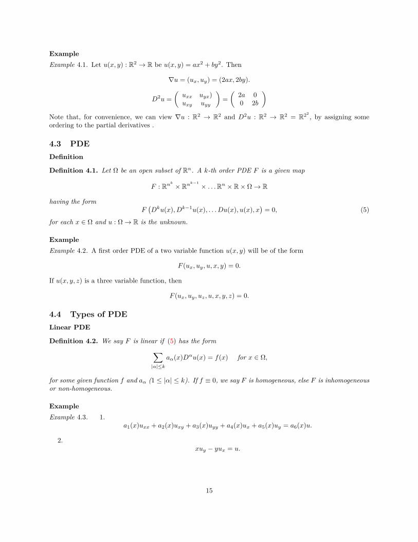
ExampleExample 4.1. Let u(x, y) : R2 → R be u(x, y) = ax2 + by2. Then
∇u = (ux, uy) = (2ax, 2by).
D2u =(uxx uyx)uxy uyy
)=(
2a 00 2b
)Note that, for convenience, we can view ∇u : R2 → R2 and D2u : R2 → R2 = R22 , by assigning someordering to the partial derivatives .
4.3 PDEDefinition
Definition 4.1. Let Ω be an open subset of Rn. A k-th order PDE F is a given map
F : Rnk
× Rnk−1× . . .Rn × R× Ω→ R
having the formF(Dku(x), Dk−1u(x), . . . Du(x), u(x), x
)= 0, (5)
for each x ∈ Ω and u : Ω→ R is the unknown.
ExampleExample 4.2. A first order PDE of a two variable function u(x, y) will be of the form
F (ux, uy, u, x, y) = 0.
If u(x, y, z) is a three variable function, then
F (ux, uy, uz, u, x, y, z) = 0.
4.4 Types of PDELinear PDE
Definition 4.2. We say F is linear if (5) has the form∑|α|≤k
aα(x)Dαu(x) = f(x) for x ∈ Ω,
for some given function f and aα (1 ≤ |α| ≤ k). If f ≡ 0, we say F is homogeneous, else F is inhomogeneousor non-homogeneous.
ExampleExample 4.3. 1.
a1(x)uxx + a2(x)uxy + a3(x)uyy + a4(x)ux + a5(x)uy = a6(x)u.
2.xuy − yux = u.
15

Semilinear PDE
Definition 4.3. F is said to be semilinear, if it is linear in the highest order, i.e., F has the form∑|α|=k
aα(x)Dαu(x) + a0(Dk−1u, . . . ,Du, u, x) = 0.
Example 4.4.ux + uy − u2.
Quasi and Non-linear
Definition 4.4. We say F is quasilinear if it has the form∑|α|=k
aα(Dk−1u(x), . . . , Du(x), u(x), x)Dαu
+a0(Dk−1u, . . . ,Du, u, x) = 0.
Finally, we say F is fully nonlinear if F is neither of the earlier form.
Example 4.5. ux + uuy − u2 is quasilinear and uxuy − u is nonlinear.
4.5 PDE-SolutionNotion of Solution
Definition 4.5. We say u : Ω→ R is a solution to the k-th order PDE (5),
• if u is k-times differentiable with the k-th derivative being continuous
• and u satisfies the equation (5).
Henceforth, whenever we refer to a function as smooth, we mean that we are given as much differentiabilityand continuity as we need.
4.6 Well PosednessBVP, IVP and Well-posedness
• A problem involving a PDE could be a boundary-value problem (we look for a solution with prescribedboundary value).
• or a initial value problem (a solution whose value at initial time is known).
A BVP or IVP is said to be well-posed, in the sense of Hadamard, if(a) has a solution (existence)(b) the solution is unique (uniqueness)(c) the solution depends continuously on the data given (stability).
16

5 Lecture - 275.1 First order PDEFirst Order PDE: Origin
Let A ⊂ R2 be an open subset. Consideru : R2 ×A→ R
a two parameter family of “smooth surfaces” in R3, u(x, y, a, b), where (a, b) ∈ A. For instance, u(x, y, a, b) =(x− a)2 + (y− b)2 is a family of circles with centre at (a, b). Differentiate w.r.t x and y, we get ux(x, y, a, b)and uy(x, y, a, b), respectively. Eliminating a and b from the two equations, we get a first order PDE
F (ux, uy, u, x, y) = 0whose solutions are the given surfaces u.
ExampleConsider the family of circles
u(x, y, a, b) = (x− a)2 + (y − b)2.
Thus, ux = 2(x− a) and uy = 2(y − b) and eliminating a and b, we getu2x + u2
y − 4u = 0is a first order PDE. Do the assignments for more examples.
5.2 Solving First Order PDEMethod of Characteristics
• We restrict ourselves to a function of two variables to fix ideas (and to visualize geometrically), however,the ideas can be carried forward to functions of several variable.
• Method of characteristics is a technique to reduce a given first order PDE to a system of ODE andthen solve the ODE using known methods to obtain the solution of the first order PDE.
Linear First Order PDE
• Consider first order linear equation of two variable:a(x, y)ux + b(x, y)uy = c(x, y). (6)
• We need to find u(x, y) that solves above equation.
• This is equivalent to finding the graph (surface) S ≡ (x, y, u(x, y)) of the function u in R3.
Integral SurfaceIf u is a solution of (6), at each (x, y) in the domain of u,
a(x, y)ux + b(x, y)uy = c(x, y)a(x, y)ux + b(x, y)uy − c(x, y) = 0
(a(x, y), b(x, y), c(x, y)) · (ux, uy,−1) = 0(a(x, y), b(x, y), c(x, y)) · (∇u(x, y),−1) = 0.
• But (∇u(x, y),−1) is normal to S at the point (x, y).
• Hence, the coefficients (a(x, y), b(x, y), c(x, y)) are perpendicular to the normal.
• Thus, the coefficients (a(x, y), b(x, y), c(x, y)) lie on the tangent plane to S at (x, y, u(x, y)).
17

Characteristic Equations
• Solving the given first order linear PDEF is finding the surface S for which (a(x, y), b(x, y), c(x, y)) lieon the tangent plane to S at (x, y, z).
• The surface is the union of curves which satisfy the property of S.
• Thus, for any curve Γ ⊂ S such that at each point of Γ, the vector V (x, y) = (a(x, y), b(x, y), c(x, y) istangent to the curve.
• Parametrizing the curve Γ by the variable s, we see that we are looking for the curve Γ = x(s), y(s), z(s) ⊂R3 such that
dx
ds= a(x(s), y(s)), dy
ds= b(x(s), y(s)),
and dz
ds= c(x(s), y(s)).
Example-Transport EquationThe three ODE’s obtained are called characteristic equations. The union of these characteristic (integral)
curves give us the integral surface.Example: Consider the linear transport equation, for a given constant a,
ut + aux = 0, x ∈ R and t ∈ (0,∞).
Thus, the vector field V (x, t) = (a, 1, 0). The characteristic equations are
dx
ds= a,
dt
ds= 1, and dz
ds= 0.
Solving Transport EquationSolving the 3 ODE’s, we get
x(s) = as+ c1, t(s) = s+ c2, and z(s) = c3.
Eliminating the parameter s, we get the curves (lines) x− at = a constant and z = a constant.z = u(x, t) is constant along the lines x− at = a constant.That is, z is a function of x− at, it changes value only when you switch between the lines. x− at. Thus,
for any function g (smooth enough)u(x, t) = g(x− at)
is a general solution of the transport equation. Because,
ut + aux = g′(x− at)(−a) + ag′(x− at) = 0.
Also, u(x, 0) = g(x).
6 Lecture - 286.1 Transport EquationInhomogeneous Transport Equation
Given a constant a ∈ R and a function f(x, t) , we wish to solve the inhomogeneous linear transportequation,
ut(x, t) + aux(x, t) = f(x, t), x ∈ R and t ∈ (0,∞).
18

As before, the first two ODE will give the projection of characteristic curve in the xt plane, x − at =a constant, and the third ODE becomes
dz(s)ds
= f(x(s), t(s)).
Let’s say we need to find the value of u at the point (x0, t0). The line passing through (x0, t0) with slope1/a is given by the equation x− at = ξ, where ξ = x0 − at0.
If z has to be on the integral curve, then z(s) = u(ξ + as, s).Hence set z(s) := u(ξ + as, s) and let γ(s) = ξ + as be the line joining (ξ, 0) and (x0, t0) as s varies from
0 to t0.The third ODE becomes,
dz(s)ds
= f(γ(s), s) = f(ξ + as, s).
Integrating both sides from 0 to t0, we get∫ t0
0f(x0 − a(t0 − s), s) ds = z(t0)− z(0)
= u(x0, t0)− u(x0 − at0, 0).
Thus,
u(x, t) = u(x− at, 0) +∫ t
0f(x− a(t− s), s) ds.
6.2 Cauchy ProblemCauchy Problem
• Recall that the general solution of the transport equation depends on the value of u at time t = 0, i.e.,the value of u on the curve (x, 0) in the xt-plane.
• Thus, the problem of finding a function u satisfying the first order PDE
a(x, y)ux + b(x, y)uy = c(x, y).
such that u is known on a curve Γ in the xt-plane is called the Cauchy problem.
• The question that arises at this moment is that: Does the knowledge of u on any curve Γ lead tosolving the first order PDE.
• The answer is: No.
Non-Characteristic Boundary Data
• Suppose, in the transport problem, we choose the curve Γ = (x, t) | x − at = 0, then we had noinformation to conclude u off the line x− at = 0.
• The characteristic curves should emanate from Γ to determine u.
• Thus, only those curves are allowed which are not characteristic curves, i.e., (a, b) is nowhere tangentto the curve.
19

Definition 6.1. We say Γ = γ1(r), γ2(r) ⊂ R2 is noncharacteristic for the Cauchy problema(x, y)ux + b(x, y)uy = c(x, y) (x, y) ∈ R2
u = φ on Γ
if Γ is nowhere tangent to (a(γ1, γ2), b(γ1, γ2)), i.e.,
(a(γ1, γ2), b(γ1, γ2)) · (−γ′2, γ′1) 6= 0.
If Γ is not noncharacteristic, then the Cauchy problem is not well-posed.
Transport Equation: IVPFor any given (smooth enough) function φ : R→ R,
ut + aux = 0 x ∈ R and t ∈ (0,∞)u(x, 0) = φ(x) x ∈ R.
We know that the general solution of the transport equation is u(x, t) = g(x − at) for some g. In the IVP,in addition, we want the initial condition u(x, 0) to be satisfied. Thus,
u(x, 0) = g(x) = φ(x).
Thus, by choosing g = φ, we get the precise solution of the IVP.Let Γ be the (boundary) curve where the initial value is given, i.e., Γ ≡ (x, 0), the x-axis of xt-plane.We have been given the value of u on Γ. Thus, (Γ, φ) = (x, 0, φ(x)) is the known curve on the solution
surface of u.We parametrize the curve Γ with r-variable, i.e., Γ = γ1(r), γ2(r) = (r, 0).Γ is non-characteristic, because (a, 1) · (0, 1) = 1 6= 0.Thus, in this setup the ODE’s are:
dx(r, s)ds
= a,dt(r, s)ds
= 1, and dz(r, s)ds
= 0
with initial conditions,x(r, 0) = r, t(r, 0) = 0, and z(r, s) = φ(r).
Solving the ODE’s, we get
x(r, s) = as+ c1(r), t(r, s) = s+ c2(r)
and z(r, s) = c3(r) with initial conditions
x(r, 0) = c1(r) = r
t(r, 0) = c2(r) = 0, and z(r, 0) = c3(r) = φ(r).
Therefore,x(r, s) = as+ r, t(r, s) = s, and z(r, s) = φ(r).
We solve for r, s in terms of x, t and set u(x, t) = z(r(x, t), s(x, t)).
r(x, t) = x− at and s(x, t) = t.
Therefore, u(x, t) = z(r, s) = φ(r) = φ(x− at).
20
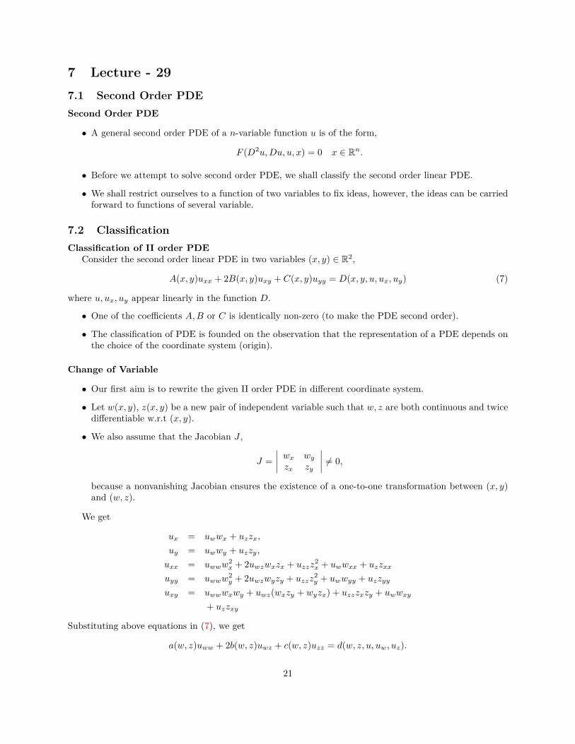
7 Lecture - 297.1 Second Order PDESecond Order PDE
• A general second order PDE of a n-variable function u is of the form,
F (D2u,Du, u, x) = 0 x ∈ Rn.
• Before we attempt to solve second order PDE, we shall classify the second order linear PDE.
• We shall restrict ourselves to a function of two variables to fix ideas, however, the ideas can be carriedforward to functions of several variable.
7.2 ClassificationClassification of II order PDE
Consider the second order linear PDE in two variables (x, y) ∈ R2,
A(x, y)uxx + 2B(x, y)uxy + C(x, y)uyy = D(x, y, u, ux, uy) (7)
where u, ux, uy appear linearly in the function D.
• One of the coefficients A,B or C is identically non-zero (to make the PDE second order).
• The classification of PDE is founded on the observation that the representation of a PDE depends onthe choice of the coordinate system (origin).
Change of Variable
• Our first aim is to rewrite the given II order PDE in different coordinate system.
• Let w(x, y), z(x, y) be a new pair of independent variable such that w, z are both continuous and twicedifferentiable w.r.t (x, y).
• We also assume that the Jacobian J ,
J =∣∣∣∣ wx wyzx zy
∣∣∣∣ 6= 0,
because a nonvanishing Jacobian ensures the existence of a one-to-one transformation between (x, y)and (w, z).
We get
ux = uwwx + uzzx,
uy = uwwy + uzzy,
uxx = uwww2x + 2uwzwxzx + uzzz
2x + uwwxx + uzzxx
uyy = uwww2y + 2uwzwyzy + uzzz
2y + uwwyy + uzzyy
uxy = uwwwxwy + uwz(wxzy + wyzx) + uzzzxzy + uwwxy
+ uzzxy
Substituting above equations in (7), we get
a(w, z)uww + 2b(w, z)uwz + c(w, z)uzz = d(w, z, u, uw, uz).
21

where D transforms in to d and
a(w, z) = Aw2x + 2Bwxwy + Cw2
y
b(w, z) = Awxzx +B(wxzy + wyzx) + Cwyzy
c(w, z) = Az2x + 2Bzxzy + Cz2
y .
• The coefficients in the new coordinate system satisfy
b2 − ac = (B2 −AC)J2.
• Since J 6= 0, we observe that the sign of the discriminant, b2−ac and B2−AC, of the PDE is invariantunder change of variable.
• We classify a second order linear PDE based on the sign of its discriminant d = B2 −AC.
We say a PDE is of
• hyperbolic type if d > 0,
• parabolic type if d = 0 and
• elliptic type if d < 0.
The motivation for these names are no indication of the geometry of the solution of the PDE, but just acorrespondence with the corresponding second degree algebraic equation
Ax2 +Bxy + Cy2 +Dx+ Ey + F = 0.
Let d = B2 − AC be the discriminant of the algebraic equation and the curve represented by the equationis a
• hyperbola if d > 0,
• parabola if d = 0 and
• ellipse if d < 0.
• The classification of PDE is dependent on its coefficients, which may vary from region to region.
• For constant coefficients, the type of PDE remains unchanged throughout the region.
• However, for variable coefficients, the PDE may change its classification from region to region.
Example 7.1. Tricomi equationuxx + xuyy = 0.
The discriminant of the Tricomi equation is d = −x.It is hyperbolic when x < 0 and elliptic when x > 0. But on the y-axis (x = 0), the equation degeneratesto uxx = 0 and it is a line. PDE’s are not defined on a line, then they degenerate to ODE’s. We say it isdegenerately parabolic when x = 0, i.e., on y-axis.
22

7.3 Standard FormsStandard or Canonical Form
The advantage of above classification is thatit helps us in reducing a given PDE into simple forms.How?Given a PDE, compute the sign of the discriminant B2 −ACand depending on its classification we can choose a coordinate transformation (w, z) such that
• a = c = 0 for hyperbolic,
• a = b = 0 or c = b = 0 for parabolic and
• a = c and b = 0 for elliptic type.
• If the given second order PDE (7) is such that A = C = 0, then (7) is of hyperbolic type and a divisionby 2B (since B 6= 0) gives
uxy = D(x, y, u, ux, uy)
where D = D/2B. The above form is the first standard form of second order hyperbolic equation.
• If we introduce the linear change of variable X = x+ y and Y = x− y in the first standard form, weget the second standard form of hyperbolic PDE
uXX − uY Y = D(X,Y, u, uX , uY ).
• If the given second order PDE (7) is such that A = B = 0, then (7) is of parabolic type and a divisionby C (since C 6= 0) gives
uyy = D(x, y, u, ux, uy)
where D = D/C. The above form is the standard form of second order parabolic equation.
• If the given second order PDE (7) is such that A = C and B = 0, then (7) is of elliptic type and adivision by A (since A 6= 0) gives
uxx + uyy = D(x, y, u, ux, uy)
where D = D/A. The above form is the standard form of second order elliptic equation.
• Note that the standard forms (except hyperbolic of first kind) of a second order linear PDE areexpressions with no mixed derivatives.
• These classification idea can be generalised to a n variable quasilinear second order PDE, since Dplayed no crucial role here.
How to reduce to standard form?Consider a second order PDE not in standard form.We look for transformation w = w(x, y) and z = z(x, y), with non-vanishing Jacobian, such that the
reduced form is the standard form. Recall that,
a(w, z) = Aw2x + 2Bwxwy + Cw2
y
b(w, z) = Awxzx +B(wxzy + wyzx) + Cwyzy
c(w, z) = Az2x + 2Bzxzy + Cz2
y .
23

HyperbolicIf B2 − AC > 0, then to make a = c = 0, we need that wx/wy and zx/zy are roots of the quadratic
equation Aξ2 + 2Bξ + C = 0.
ξ = −B ±√B2 −ACA
.
Thus,wxwy
= −B +√B2 −ACA
and zxzy
= −B −√B2 −ACA
.
Along the curve such that w = a constant, we have
0 = dw
dx= wy
dy
dx+ wx
and hence dydx = −wx
wy. Similarly, dy
dx = −zx
zy. The characteristic curve is given by dy
dx = −ξ.In the parabolic case, B2 − AC = 0 and we have ξ = −B/A. Thus, we solve along the curve w = a
constant,dy
dx= −ξ
and choose z such that the Jacobian J 6= 0.In the elliptic case, B2 −AC < 0. Thus, ξ has a real and imaginary part. We solve
dy
dx= −ξ
and choose the real part of the solution to be w and imaginary part to be the z.
8 Lecture - 308.1 Three Basic Linear PDEThree Basic Second Order Linear PDE
For any x ∈ Rn,
• The Laplace equation, ∆u(x) = 0 where ∆ :=∑ni=1
∂2
∂x2i
is the trace of the Hessian matrix. The Poissonequation, ∆u(x) = f(x).
• The heat equation for a homogeneous material is ut(x, t)− c2∆u(x, t) = 0, for t ≥ 0 and c is a non-zeroconstant.
• The wave equation with normalised constants is
utt(x, t)− c2∆u(x, t) = 0
for t ≥ 0.
Superposition PrincipleThe three basic II order PDE are linear and satisfies the superposition principle: If u1, u2 are solutions
of these equations, thenα1u1 + α2u2
is also a solution, for all constants α1, α2 ∈ R.
24
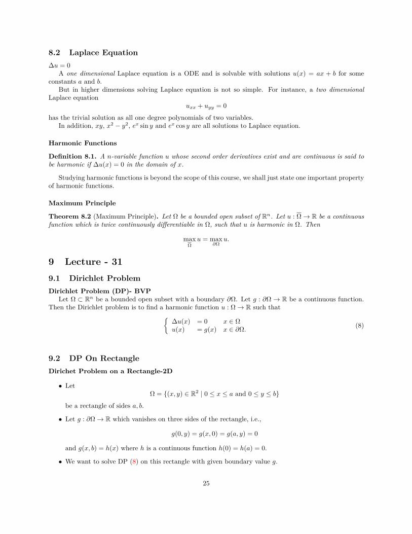
8.2 Laplace Equation∆u = 0
A one dimensional Laplace equation is a ODE and is solvable with solutions u(x) = ax + b for someconstants a and b.
But in higher dimensions solving Laplace equation is not so simple. For instance, a two dimensionalLaplace equation
uxx + uyy = 0
has the trivial solution as all one degree polynomials of two variables.In addition, xy, x2 − y2, ex sin y and ex cos y are all solutions to Laplace equation.
Harmonic Functions
Definition 8.1. A n-variable function u whose second order derivatives exist and are continuous is said tobe harmonic if ∆u(x) = 0 in the domain of x.
Studying harmonic functions is beyond the scope of this course, we shall just state one important propertyof harmonic functions.
Maximum Principle
Theorem 8.2 (Maximum Principle). Let Ω be a bounded open subset of Rn. Let u : Ω→ R be a continuousfunction which is twice continuously differentiable in Ω, such that u is harmonic in Ω. Then
maxΩ
u = max∂Ω
u.
9 Lecture - 319.1 Dirichlet ProblemDirichlet Problem (DP)- BVP
Let Ω ⊂ Rn be a bounded open subset with a boundary ∂Ω. Let g : ∂Ω → R be a continuous function.Then the Dirichlet problem is to find a harmonic function u : Ω→ R such that
∆u(x) = 0 x ∈ Ωu(x) = g(x) x ∈ ∂Ω. (8)
9.2 DP On RectangleDirichet Problem on a Rectangle-2D
• LetΩ = (x, y) ∈ R2 | 0 ≤ x ≤ a and 0 ≤ y ≤ b
be a rectangle of sides a, b.
• Let g : ∂Ω→ R which vanishes on three sides of the rectangle, i.e.,
g(0, y) = g(x, 0) = g(a, y) = 0
and g(x, b) = h(x) where h is a continuous function h(0) = h(a) = 0.
• We want to solve DP (8) on this rectangle with given boundary value g.
25
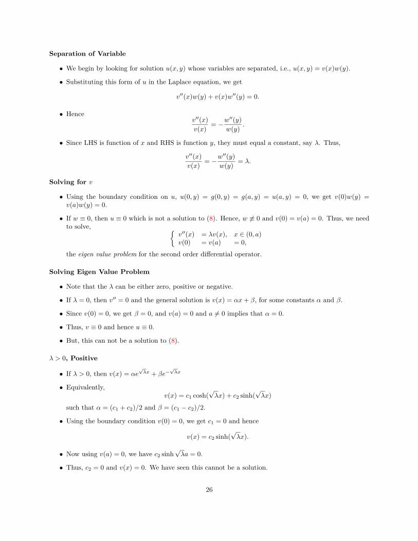
Separation of Variable
• We begin by looking for solution u(x, y) whose variables are separated, i.e., u(x, y) = v(x)w(y).
• Substituting this form of u in the Laplace equation, we get
v′′(x)w(y) + v(x)w′′(y) = 0.
• Hencev′′(x)v(x) = −w
′′(y)w(y) .
• Since LHS is function of x and RHS is function y, they must equal a constant, say λ. Thus,
v′′(x)v(x) = −w
′′(y)w(y) = λ.
Solving for v
• Using the boundary condition on u, u(0, y) = g(0, y) = g(a, y) = u(a, y) = 0, we get v(0)w(y) =v(a)w(y) = 0.
• If w ≡ 0, then u ≡ 0 which is not a solution to (8). Hence, w 6≡ 0 and v(0) = v(a) = 0. Thus, we needto solve,
v′′(x) = λv(x), x ∈ (0, a)v(0) = v(a) = 0,
the eigen value problem for the second order differential operator.
Solving Eigen Value Problem
• Note that the λ can be either zero, positive or negative.
• If λ = 0, then v′′ = 0 and the general solution is v(x) = αx+ β, for some constants α and β.
• Since v(0) = 0, we get β = 0, and v(a) = 0 and a 6= 0 implies that α = 0.
• Thus, v ≡ 0 and hence u ≡ 0.
• But, this can not be a solution to (8).
λ > 0, Positive
• If λ > 0, then v(x) = αe√λx + βe−
√λx
• Equivalently,v(x) = c1 cosh(
√λx) + c2 sinh(
√λx)
such that α = (c1 + c2)/2 and β = (c1 − c2)/2.
• Using the boundary condition v(0) = 0, we get c1 = 0 and hence
v(x) = c2 sinh(√λx).
• Now using v(a) = 0, we have c2 sinh√λa = 0.
• Thus, c2 = 0 and v(x) = 0. We have seen this cannot be a solution.
26

λ < 0, Negative
• If λ < 0, then set ω =√−λ
• We need to solve v′′(x) + ω2v(x) = 0 x ∈ (0, a)v(0) = v(a) = 0.
• The general solution isv(x) = α cos(ωx) + β sin(ωx).
• Using the boundary condition v(0) = 0, we get α = 0 and hence v(x) = β sin(ωx).
• Now using v(a) = 0, we have β sinωa = 0.
• Thus, either β = 0 or sinωa = 0. But β = 0 does not yield a solution.
• Hence ωa = kπ or ω = kπ/a, for all non-zero k ∈ Z.
• Hence, for each k ∈ N, there is a solution (vk, λk) for (8), with
vk(x) = βk sin(kπx
a
),
for some constant bk and λk = −(kπ/a)2.
• We have solved for v. it now remains to solve w for these λk.
• For each k ∈ N, we solve for wk in the ODEw′′k(y) =
(kπa
)2wk(y), y ∈ (0, b)
w(0) = 0.
Thus, wk(y) = ck sinh(kπy/a).
General Solution to DP
• For each k ∈ N,
uk = δk sin(kπx
a
)sinh
(kπy
a
)is a solution to (8).
• The general solution is of the form (principle of superposition) (convergence?)
u(x, y) =∞∑k=1
δk sin(kπx
a
)sinh
(kπy
a
).
Final Solution to DP on Rectangle
• We shall now use the condition u(x, b) = h(x) to find the solution to the Dirichlet problem (8).
•
h(x) = u(x, b) =∞∑k=1
δk sinh(kπb
a
)sin(kπx
a
).
• Since h(0) = h(a) = 0, we know that h admits a Fourier Sine series.
• Thus δk sinh(kπba
)is the k-th Fourier sine coefficient of h, i.e.,
δk =(
sinh(kπb
a
))−1 2a
∫ a
0h(x) sin
(kπx
a
).
27

10 Lecture - 3210.1 Laplace EquationLaplacian in Polar Coordinates
• Now that we have solved the Dirichlet problem in a 2D rectangular domain, we intend to solve theDirichlet problem in a 2D disk.
• The Laplace operator in polar coordinates (2 dimensions),
∆ := 1r
∂
∂r
(r∂
∂r
)+ 1r2
∂2
∂θ2
where r is the magnitude component and θ is the direction component.
10.2 Laplacian on a 2D-DiskDirichet Problem on a Disk-2D
• Consider the unit disk Ω in R2,
Ω = (x, y) ∈ R2 | x2 + y2 < 1
and ∂Ω is the circle of radius one.
• The DP is to find u(r, θ) : Ω→ R which is well-behaved near r = 0, such that1r∂∂r
(r ∂u∂r
)+ 1
r2∂2u∂θ2 = 0 in Ω
u(r, θ + 2π) = u(r, θ) in Ωu(1, θ) = g(θ) on ∂Ω
(9)
where g is a 2π periodic function.
Separation of Variable
• We will look for solution u(r, θ) whose variables can be separated, i.e., u(r, θ) = v(r)w(θ) with both vand w non-zero.
• Substituting it in the polar form of Laplacian, we get
w
r
d
dr
(rdv
dr
)+ v
r2d2w
dθ2 = 0
• and hence−rv
d
dr
(rdv
dr
)= 1w
(d2w
dθ2
).
• Since LHS is a function of r and RHS is a function of θ, they must equal a constant, say λ.
28
Solving for w
• We need to solve the eigen value problem,w′′(θ)− λw(θ) = 0 θ ∈ Rw(θ + 2π) = w(θ) ∀θ.
• Note that the λ can be either zero, positive or negative.
• If λ = 0, then w′′ = 0 and the general solution is w(θ) = αθ + β, for some constants α and β. Usingthe periodicity of w,
αθ + β = w(θ) = w(θ + 2π) = αθ + 2απ + β
implies that α = 0. Thus, the pair λ = 0 and w(θ) = β is a solution.
λ > 0, Positive
• If λ > 0, thenw(θ) = αe
√λθ + βe−
√λθ.
• If either of α and β is non-zero, then w(θ)→ ±∞ as θ →∞, which contradicts the periodicity of w.
• Thus, α = β = 0 and w ≡ 0, which cannot be a solution.
λ < 0, Negative
• If λ < 0, then set ω =√−λ and the equation becomes
w′′(θ) + ω2w(θ) = 0 θ ∈ Rw(θ + 2π) = w(θ) ∀θ
• Its general solution isw(θ) = α cos(ωθ) + β sin(ωθ).
• Using the periodicity of w, we get ω = k where k is an integer.
• For each k ∈ N, we have the solution (wk, λk) where
λk = −k2 and wk(θ) = αk cos(kθ) + βk sin(kθ).
Solving for v
• For the λk’s, we solve for vk, for each k = 0, 1, 2, . . .,
rd
dr
(rdvkdr
)= k2vk.
• For k = 0, we get v0(r) = α log r + β. But log r blows up as r → 0 and we wanted a u well behavednear origin.
• Thus, we must have the α = 0. Hence v0 ≡ β.
29

Cauchy-Euler Equation
• For k ∈ N, we need to solve for vk in
rd
dr
(rdvkdr
)= k2vk.
Use the change of variable r = es. Then es dsdr = 1 and ddr = d
dsdsdr = 1
esdds . Hence r ddr = d
ds .
• vk(es) = αeks + βe−ks.
• vk(r) = αrk + βr−k.
• Since r−k blows up as r → 0, we must have β = 0.
• Thus, vk = αrk. Therefore, for each k = 0, 1, 2, . . .,
uk(r, θ) = akrk cos(kθ) + bkr
k sin(kθ).
Final Solution for DP on Disk
• The general solution is
u(r, θ) = a0
2 +∞∑k=1
(akr
k cos(kθ) + bkrk sin(kθ)
).
• To find the constants, we use u(1, θ) = g(θ), hence
g(θ) = a0
2 +∞∑k=1
[ak cos(kθ) + bk sin(kθ)] .
• Since g is 2π-periodic it admits a Fourier series expansion and hence
ak = 1π
∫ π
−πg(θ) cos(kθ) dθ,
bk = 1π
∫ π
−πg(θ) sin(kθ) dθ.
11 Lecture - 3311.1 Laplace EquationLaplacian in Spherical Coordinates
• Now that we have solved the Dirichlet problem in a 2D disk, we intend to solve the Dirichlet problemin a 3D sphere.
• The Laplace operator in spherical coordinates (3 dimensions),
∆ := 1r2
∂
∂r
(r2 ∂
∂r
)+ 1r2 sin θ
∂
∂θ
(sin θ ∂
∂θ
)+ 1r2 sin2 θ
∂2
∂φ2 .
where r is the magnitude component, θ is the inclination (elevation) in the vertical plane and φ is theazimuth angle (in the direction in horizontal plane.
30

11.2 Laplacian on a 3D-SphereLaplacian on a Sphere-3D
• Consider the unit sphere Ω in R3,
Ω = (x, y, z) ∈ R3 | x2 + y2 + z2 < 1
and ∂Ω is the boundary of sphere of radius one.
• The DP is to find u(r, θ, φ) : Ω→ R which is well-behaved near r = 0, such that1r2
∂∂r
(r2 ∂u
∂r
)+ 1
r2 sin θ∂∂θ
(sin θ ∂u∂θ
)+ 1r2 sin2 θ
∂2u∂φ2 = 0 in Ω
u(r, θ + 2π, φ+ 2π) = u(r, θ, φ) in Ωu(1, θ, φ) = g(θ, φ) on ∂Ω
(10)
where g is a 2π periodic function in both variables.
Separation of Variable
• We will look for solution u(r, θ, φ) whose variables can be separated, i.e., u(r, θ, φ) = v(r)w(θ)z(φ) withv, w and z non-zero.
• Substituting it in the spherical form of Laplacian, we get
wz
r2d
dr
(r2 dv
dr
)+ vz
r2 sin θd
dθ
(sin θdw
dθ
)+ vw
r2 sin2 θ
d2z
dφ2 = 0
• and hence1v
d
dr
(r2 dv
dr
)= −1w sin θ
d
dθ
(sin θdw
dθ
)− 1z sin2 θ
d2z
dφ2 .
• Since LHS is a function of r and RHS is a function of (θ, φ), they must equal a constant, say λ.
Azimuthal Symmetry
• If Azimuthal symmetry is present then z(φ) is constant and hence dzdφ = 0.
• We need to solve for w,sin θw′′(θ) + cos θw′(θ) + λ sin θw(θ) = 0 θ ∈ R
w(θ + 2π) = w(θ) ∀θ.
• Set x = cos θ.
• Then dxdθ = − sin θ
•w′(θ) = − sin θdw
dxand w′′(θ) = sin2 θ
d2w
dx2 − cos θdwdx
31

Legendre Equation
• In the new variable x, we get the Legendre equation
(1− x2)w′′(x)− 2xw′(x) + λw(x) = 0 x ∈ [−1, 1].
• We have already seen that this is a singular problem (while studying S-L problems). For each k ∈N ∪ 0, we have the solution (wk, λk) where
λk = k(k + 1) and wk(θ) = Pk(cos θ).
Solving for v
• For the λk’s, we solve for vk, for each k = 0, 1, 2, . . .,d
dr
(r2 dvkdr
)= k(k + 1)vk.
• For k = 0, we get v0(r) = −α/r+ β. But 1/r blows up as r → 0 and we wanted a u well behaved nearorigin.
• Thus, we must have the α = 0. Hence v0 ≡ β.
Cauchy-Euler Equation
• For k ∈ N, we need to solve for vk ind
dr
(r2 dvkdr
)= k(k + 1)vk.
Use the change of variable r = es. Then es dsdr = 1 and ddr = d
dsdsdr = 1
esdds . Hence r ddr = d
ds .
• solving for m in the quadratic equation m2 +m = k(k + 1).
• m1 = k and m2 = −k − 1.
• vk(es) = αeks + βe(−k−1)s.
• vk(r) = αrk + βr−k−1.
• Since r−k−1 blows up as r → 0, we must have β = 0.
• Thus, vk = αrk. Therefore, for each k = 0, 1, 2, . . .,
uk(r, θ, φ) = akrkPk(cos θ).
Final Solution for Laplacian on Sphere
• The general solution is
u(r, θ, φ) =∞∑k=0
akrkPk(cos θ).
• Since we have azimuthal symmetry, g(θ, φ) = g(θ).
• To find the constants, we use u(1, θ, φ) = g(θ), hence
g(θ) =∞∑k=0
akPk(cos θ).
• Using the orthogonality of Pk, we have
ak = 2k + 12
∫ π
−πg(θ)Pk(cos θ) dθ.
32

12 Lecture-3412.1 Eigenvalues of LaplacianEigenvalue Problem of Laplacian
• Recall that we did the eigenvalue problem for the Sturm-Liouville operator, which was one-dimensional.
• A similar result is true for Laplacian in all dimensions. However, we shall just state in two dimensions.For a given open bounded subset Ω ⊂ R2, the Dirichlet eigenvalue problem,
−∆u(x, y) = λu(x, y) (x, y) ∈ Ωu(x, y) = 0 (x, y) ∈ ∂Ω.
Eigenvalue and Eigen function
• Note that, for all λ ∈ R, zero is a trivial solution of the Laplacian.
• Thus, we are interested in non-zero λ’s for which the Laplacian has non-trivial solutions. Such an λ iscalled the eigenvalue and corresponding solution uλ is called the eigen function.
• Note that if uλ is an eigen function corresponding to λ, then αuλ, for all α ∈ R, is also an eigenfunction corresponding to λ.
Existence
• Let W be the real vector space of all u : Ω→ R continuous (smooth, as required) functions such thatu(x, y) = 0 on ∂Ω.
• For each eigenvalue λ of the Laplacian, we define the subspace of W as
Wλ = u ∈W | u solves Dirichlet EVP for given λ.
Theorem 12.1. There exists an increasing sequence of positive numbers 0 < λ1 < λ2 < λ3 < . . . < λn < . . .with λn →∞ which are eigenvalues of the Laplacian and Wn = Wλn
is finite dimensional. Conversely, anysolution u of the Laplacian is in Wn, for some n.
12.2 Computing EigenvaluesSpecific Domains Ω
• Though the theorem assures the existence of eigenvalues for Laplacian, it is usually difficult to computethem for a given Ω.
• In this course, we shall compute the eigenvalues when Ω is a 2D-rectangle and a 2D-disk.
12.3 In RectangleEigenvalues of Laplacian in Rectangle
• Let the rectangle be Ω = (x, y) ∈ R2 | 0 < x < a, 0 < y < b.
• we wish to solve the Dirichlet EVP in the rectangle Ω−∆u(x, y) = λu(x, y) (x, y) ∈ Ω
u(x, y) = 0 (x, y) ∈ ∂Ω.
• The boundary condition amounts to saying
u(x, 0) = u(a, y) = u(x, b) = u(0, y) = 0.
33
Separation Of Variable
• We look for solutions of the form u(x, y) = v(x)w(y) (variable separated).
• Substituting u in separated form in the equation, we get
−v′′(x)w(y)− v(x)w′′(y) = λv(x)w(y).
• Hence−v′′(x)v(x) = λ+ w′′(y)
w(y) .
• Since LHS is function of x and RHS is function y and are equal they must be some constant, say µ.
• We need to solve the EVP’s
−v′′(x) = µv(x) and − w′′(y) = (λ− µ)w(y)
• under the boundary conditions v(0) = v(a) = 0 and w(0) = w(b) = 0.
Solving for v
• As seen before, while solving for v, we have trivial solutions for µ ≤ 0.
• If µ > 0, then v(x) = c1 cos(√µx) + c2 sin(√µx).
• Using the boundary condition v(0) = 0, we get c1 = 0. Now using v(a) = 0, we have c2 sin√µa = 0.Thus, either c2 = 0 or sin√µa = 0.
• We have non-trivial solution, if c2 6= 0, then √µa = kπ or √µ = kπ/a, for k ∈ Z.
• For each k ∈ N, we have vk(x) = sin(kπx/a) and µk = (kπ/a)2.
Solving for w
• We solve for w for each µk.
• For each k, l ∈ N, we have wkl(y) = sin(lπy/b) and λkl = (kπ/a)2 + (lπ/b)2.
• For each k, l ∈ N, we haveukl(x, y) = sin(kπx/a) sin(lπy/b)
and λkl = (kπ/a)2 + (lπ/b)2.
12.4 In DiskEigenvalues of Laplacian in Disk
• Let the disk of radius a be Ω = (x, y) ∈ R2 | x2 + y2 < a2.
• We wish to solve the Dirichlet EVP in the disk Ω−1r
∂∂r
(r ∂u∂r
)− 1
r2∂2u∂θ2 = λu(r, θ) (r, θ) ∈ Ωu(θ) = u(θ + 2π) θ ∈ R
u(a, θ) = 0 θ ∈ R.
• We look for solutions of the form u(r, θ) = v(r)w(θ) (variable separated).
34

• Substituting u in separated form in the equation, we get
−wr
d
dr
(rdv
dr
)− v
r2w′′(θ) = λv(r)w(θ).
• Hence dividing by vw and multiplying by r2, we get
− rv
d
dr
(rdv
dr
)− 1ww′′(θ) = λr2.
•r
v
d
dr
(rdv
dr
)+ λr2 = −1
ww′′(θ) = µ.
• Solving for non-trivial w, using the periodicity of w, we get for µ = 0, w(θ) = a02 and for each k ∈ N,
µ = k2 andw(θ) = ak cos kθ + bk sin kθ.
Solving for v
• For each k ∈ N ∪ 0, we have the equation,
rd
dr
(rdv
dr
)+ (λr2 − k2)v = 0.
• Introduce change of variable x =√λr and x2 = λr2. Then
rd
dr= x
d
dx.
• rewriting the equation in new variable y(x)) = v(r)
xd
dx
(xdy(x)dx
)+ (x2 − k2)y(x) = 0.
• Note that this none other than the Bessel’s equation.
12.5 Bessel’s FunctionZeroes of Bessel’s Function
• We already know that for each k ∈ N ∪ 0, we have the Bessel’s function Jk as a solution to theBessel’s equation.
• Recall the boundary condition on v, v(a) = 0. Thus. y(√λa) = 0.
• Hence√λa should be a zero of the Bessel’s function.
Theorem 12.2. For each non-negative integer k, Jk has infinitely many positive zeroes.
• For each k ∈ N ∪ 0, let zkl be the l-th zero of Jk.
• Hence√λa = zkl and so λkl = z2
kl/a2 and y(x) = Jk(x).
• Therefore, v(r) = Jk(zklr/a).
• For each k, l ∈ N ∪ 0, we have
ukl(r, θ) = Jk(zklr/a) sin(kθ) or Jk(zklr/a) cos(kθ)
and λkl = z2kl/a
2.
35

13 Lecture - 3513.1 1D Heat EquationOne dimensional Heat Equation
• The equation governing heat propogation in a bar of length L is
∂u
∂t= 1ρ(x)σ(x)
∂
∂x
(κ(x)∂u
∂x
)where σ(x) is the alertspecific heat at x, ρ(x) is density of bar at x and κ(x) is the thermal conductivityof the bar at x.
• If the bar is homogeneous, i.e, its properties are same at every point, then
∂u
∂t= κ
ρσ
∂2u
∂x2
with ρ, σ, κ being constants.
IVP for Heat Equation
• Let L be the length of a homogeneous rod insulated along sides and its ends are kept at zero temper-ature.
• Then the temperature u(x, t) at every point of the rod, 0 ≤ x ≤ L and time t ≥ 0 is given by theequation
∂u
∂t= c2
∂2u
∂x2
where c is a constant.
• The temperature zero at the end points is given by the Dirichlet boundary condition
u(0, t) = u(L, t) = 0.
• Also, given is the initial temperature of the rod at time t = 0, u(x, 0) = g(x), where g is given (orknown) such that g(0) = g(L) = 0.
Dirichlet Problem for Heat Equation
• Given g : [0, L]→ R such that g(0) = g(L) = 0, we look for all the solutions of the Dirichlet problem ut(x, t)− c2uxx(x, t) = 0 in (0, L)× (0,∞)u(0, t) = u(L, t) = 0 in (0,∞)
u(x, 0) = g(x) on [0, L].
• We look for u(x, t) = v(x)w(t) (variable separated).
• Substituting u in separated form in the equation, we get
v(x)w′(t) = c2v′′(x)w(t)
•w′(t)c2w(t) = v′′(x)
v(x) .
36

Dirichlet Problem for Heat Equation
• Since LHS is function of t and RHS is function x and are equal they must be some constant, say λ.Thus,
w′(t)c2w(t) = v′′(x)
v(x) = λ.
• Thus we need to solve two ODE to get v and w,
w′(t) = λc2w(t)
andv′′(x) = λv(x).
• But we already know how to solve the eigenvalue problem involving v.
Solving for v and w
• For each k ∈ N, we have the pair (λk, vk) as solutions to the EVP involving v, where λk = −(kπ)2/L2
and vk(x) = sin(kπxL
)some constants bk.
• For each k ∈ N, we solve for wk to get
lnwk(t) = λkc2t+ lnα
where α is integration constant. Thus, wk(t) = αe−(kcπ/L)2t.
• Hence,
uk(x, t) = vk(x)wk(t) = βk sin(kπx
L
)e−(kcπ/L)2t,
for some constants βk, is a solution to the heat equation.
• By superposition principle, the general solution is
u(x, t) =∞∑k=1
uk(x, t) =∞∑k=1
βk sin(kπx
L
)e−(kcπ/L)2t.
Particular Solution of Heat Equation
• We now use the initial temperature of the rod, given as g : [0, L]→ R to find the particular solution ofthe heat equation.
• We are given u(x, 0) = g(x). Thus,
g(x) = u(x, 0) =∞∑k=1
βk sin(kπx
L
)
• Since g(0) = g(L) = 0, we know that g admits a Fourier Sine expansion and hence its coefficients βkare given as
βk = 2L
∫ L
0g(x) sin
(kπx
L
).
37
13.2 Solving for Circular WireHeat Equation of a Circular Wire
• We intend solve the heat equation in a circle (circular wire) of radius one which is insulated along itssides.
• Then the temperature u(θ, t) at every point of the circle, θ ∈ R and time t ≥ 0 is given by the equation
∂u
∂t= c2
∂2u
∂θ2
where c is a constant.
• We note that now u(θ, t) is 2π-periodic in the variable θ. Thus,
u(θ + 2π, t) = u(θ, t) ∀θ ∈ R, t ≥ 0.
• Let the initial temperature of the wire at time t = 0, be u(θ, 0) = g(θ), where g is a given 2π-periodicfunction.
IVP
• Given a 2π-periodic function g : R→ R, we look for all solutions of ut(θ, t)− c2uθθ(θ, t) = 0 in R× (0,∞)u(θ + 2π, t) = u(θ, t) in R× (0,∞)
u(θ, 0) = g(θ) on R× t = 0.
• We look for u(θ, t) = v(θ)w(t) with varibales separated
• substituting for u in the equation, we get
w′(t)c2w(t) = v′′(θ)
v(θ) = λ.
Solving for v and w
• For each k ∈ N ∪ 0, the pair (λk, vk) is a solution to the EVP where λk = −k2 and
vk(θ) = ak cos(kθ) + bk sin(kθ).
• For each k ∈ N ∪ 0, we get wk(t) = αe−(kc)2t.
General Solution
• For k = 0u0(θ, t) = a0/2 (To maintain consistency with Fourier series)
and for each k ∈ N, we have
uk(θ, t) = [ak cos(kθ) + bk sin(kθ)] e−k2c2t
• Therefore, the general solution is
u(θ, t) = a0
2 +∞∑k=1
[ak cos(kθ) + bk sin(kθ)] e−k2c2t.
38

Particular Solution
• We now use the initial temperature on the circle to find the particular solution. We are given u(θ, 0) =g(θ).
• Thus,
g(θ) = u(θ, 0) = a0
2 +∞∑k=1
[ak cos(kθ) + bk sin(kθ)]
• Since g is 2π-periodic it admits a Fourier series expansion and hence
ak = 1π
∫ π
−πg(θ) cos(kθ) dθ,
bk = 1π
∫ π
−πg(θ) sin(kθ) dθ.
• Note that as t→∞ the temperature of the wire approaches a constant a0/2.
Exercises!Solve the heat equation for
• 2D Rectangle.
• 2D Disk.
14 Lecture - 3614.1 1D Wave EquationOne dimensional Wave Equation
• Let us consider a string of length L, stretched along the x-axis, with one end fixed at x = 0 and theother end being x = L.
• We assume that the string is free to move only in the vertical direction.
• The vertical displacement u(x, t) of the string at the point x and time t is governed by the equation
∂2u
∂t2= T
ρ
∂2u
∂x2
where T is the tension and ρ is the density of the string.
• Equivalently,∂2u
∂t2= c2
∂2u
∂x2
where c2 = T/ρ.
IVP for Wave Equation
• The fact that endpoints are fixed is given by the Dirichlet boundary condition
u(0, t) = u(L, t) = 0.
• Also, given is the initial position u(x, 0) = g(x) (at time t = 0)
• Initial velocity of the string at time t = 0, ut(x, 0) = h(x).
39

Dirichlet Problem for Wave Equation
• Given g, h : [0, L]→ R such that g(0) = g(L) = 0, we need to solveutt(x, t)− c2uxx(x, t) = 0 in (0, L)× (0,∞)
u(0, t) = u(L, t) = 0 in [0,∞)u(x, 0) = g(x) in [0, L]ut(x, 0) = h(x) in (0, L)
• We seek u(x, t) = v(x)w(t) (variable separated).
• Substituting u in separated form in the equation, we get
v(x)w′′(t) = c2v′′(x)w(t)
• Hencew′′(t)c2w(t) = v′′(x)
v(x) = λ.
Solving for v and w
• For each k ∈ N, we obtain the non-trivial solutions (λk, vk), where
vk(x) = sin(kπx
L
)and λk = −(kπ/L)2.
• For each k ∈ N, we solve for wk in
w′′k(t) + (kπ/L)2c2wk(t) = 0.
• Hencewk(t) = ak cos(kcπt/L) + bk sin(kcπt/L).
General Solution of Wave Equation
• For each k ∈ N, we have
uk(x, t) = [ak cos(kcπt/L) + bk sin(kcπt/L)] sin(kπx
L
)for some constants ak and bk.
• Hence, the general solution is
u(x, t) =∞∑k=1
[ak cos(kcπt/L) + bk sin(kcπt/L)] sin(kπx
L
)
• Frequency of the fundamental mode is
12π
cπ
L= c
2L =√T/ρ
2L
and the frequency of higher modes are integer multiples of the this frequency.
40

Particular Solution of Wave Equation
• We now use the initial position g and initial velocity h of the string to find the particular solution ofthe wave equation. We are given u(x, 0) = g(x) and ut(x, 0) = h(x).
• Thus,
g(x) = u(x, 0) =∞∑k=1
ak sin(kπx
L
)• Since g(0) = g(L) = 0, we know that g admits a Fourier Sine expansion and hence its coefficients ak
are given as
ak = 2L
∫ L
0g(x) sin
(kπx
L
).
• Differentiating u w.r.t t, we get
ut(x, t) =∞∑k=1
(kcπ/L) [bk cos(kcπt/L)− ak sin(kcπt/L)] sin(kπx
L
).
• Thus,
h(x) = ut(x, 0) =∞∑k=1
bkkcπ
Lsin(kπx
L
)• and
bk = 2kcπ
∫ L
0h(x) sin
(kπx
L
).
Exercises!Solve the wave equation for
• 2D Rectangle.
• 2D Disk.
15 Lecture - 3715.1 Duhamel’s PrincipleDuhamel’s Principle
• Recall that we have studied the homogeneous IVP for heat and wave equation with non-zero initialcondition.
• Duhamels’s principle states that one can obtain a solution of the inhomogeneous IVP for heat andwave from its homogeneous IVP.
41

Duhamel’s for Heat Equation
• Let us illustrate the principle for heat equation.
• Let u(x, t) be the solution of the inhomogeneous heat equation, for a given f ut(x, t)− c2∆u(x, t) = f(x, t) in Ω× (0,∞)u(x, t) = 0 in ∂Ω× (0,∞)u(x, 0) = 0 in Ω.
• Consider, for each s ∈ (0,∞), w(x, t; s) as the solution of the homogeneous problem (auxiliary) wst (x, t)− c2∆ws(x, t) = 0 in Ω× (s,∞)ws(x, t) = 0 in ∂Ω× (s,∞)ws(x, s) = f(x, s) on Ω.
• Since t ∈ (s,∞), introducing a change of variable r = t− s, we have ws(x, t) = w(x, t− s) which solves wt(x, r)− c2∆w(x, r) = 0 in Ω× (0,∞)w(x, r) = 0 in ∂Ω× (0,∞)w(x, 0) = f(x, t) on Ω.
• Duhamel’s principle states that
u(x, t) =∫ t
0ws(x, t) ds =
∫ t
0w(x, t− s) ds
Proof
• Let us prove that u defined as
u(x, t) =∫ t
0w(x, t− s) ds
solves the inhomogenous heat equation.
• Assuming w is C2, we get
ut(x, t) = ∂
∂t
∫ t
0w(x, t− s) ds
=∫ t
0wt(x, t− s) ds+ w(x, t− t)d(t)
dt
− w(x, t− 0)d(0)dt
=∫ t
0wt(x, t− s) ds+ w(x, 0).
ut(x, t) =∫ t
0wt(x, t− s) ds+ w(x, 0)
=∫ t
0wt(x, t− s) ds+ f(x, t).
42

Similarly,
∆u(x, t) =∫ t
0∆w(x, t− s) ds.
Thus,
ut − c2∆u = f(x, t) +∫ t
0
(wt(x, t− s)− c2∆w(x, t− s)
)ds
= f(x, t).
Duhamel’s for Wave Equation (Exercise!)
• The principle states that the solution u(x, t) of the inhomogeneous wave equation, for a given f utt(x, t)−∆u(x, t) = f(x, t) in Ω× (0,∞)u(x, t) = 0 in ∂Ω× (0,∞)
u(x, 0) = ut(x, 0) = 0 in Ω.
• is u(x, t) =∫ t
0 w(x, t− s) ds
• where w(x, t− s) is the solution of the homogeneous equationwtt(x, t− s)−∆w(x, t− s) = 0 in Ω× (0,∞)
w(x, t− s) = 0 in ∂Ω× (0,∞)w(x, 0) = 0 on Ωwt(x, 0) = f(x, t) on Ω.
Example
• Consider the wave equation utt(x, t)− c2uxx(x, t) = sin 3x in (0, π)× (0,∞)u(0, t) = u(π, t) = 0 in (0,∞)
u(x, 0) = ut(x, 0) = 0 in (0, π).
• We look for the solution of the homogeneous wave equationwtt(x, t)− c2wxx(x, t) = 0 in (0, π)× (0,∞)
w(0, t) = w(π, t) = 0 in (0,∞)w(x, 0) = 0 in (0, π)wt(x, 0) = sin 3x in (0, π).
Solving Homogeneous Equation
• We know that the general solution of w is
w(x, t) =∞∑k=1
[ak cos(kct) + bk sin(kct)] sin(kx)
43

• Hence
w(x, 0) =∞∑k=1
ak sin(kx) = 0.
• Thus, ak = 0, for all k.
• Also,
wt(x, 0) =∞∑k=1
bkck sin(kx) = sin 3x.
Hence, bk’s are all zeroes except k = 3 and b3 = 1/3c.
• Thus,w(x, t) = 1
3c sin(3ct) sin(3x).
Solving Inhomogeneous Equation
u(x, t) =∫ t
0w(x, t− s) ds
= 13c
∫ t
0sin(3c(t− s)) sin 3x ds
= sin 3x3c
∫ t
0sin(3c(t− s)) ds
= sin 3x cos(3c(t− s))3c |t0
= sin 3x9c2 (1− cos 3ct) .
16 Lecture - 3816.1 d’Alembert’s Formulad’Alembert’s Formula: 1D Wave Equation
• Consider the IVP utt(x, t) = c2uxx(x, t) in R× (0,∞)u(x, 0) = g(x) in R× t = 0ut(x, 0) = h(x) in R× t = 0,
where g, h : R→ R are given functions.
• Note that the PDE can be factored as(∂
∂t+ c
∂
∂x
)(∂
∂t− c ∂
∂x
)u = utt − c2uxx = 0.
• We set v(x, t) =(∂∂t − c
∂∂x
)u(x, t) and hence
vt(x, t) + cvx(x, t) = 0 in R× (0,∞).
44

Solve Two Transport Equations
• Notice that the first order PDE obtained is in the form of homogeneous transport equation, which weknow to solve.
• Hence, for some smooth function f ,v(x, t) = f(x− ct)
and f(x) := v(x, 0).
• Using v in the original equation, we get the inhomogeneous transport equation,
ut(x, t)− cux(x, t) = f(x− ct).
• Recall the formula for inhomogenoeus TE
u(x, t) = g(x− at) +∫ t
0f(x− a(t− s), s) ds.
• Since u(x, 0) = g(x) and a = −c, in our case the solution reduces to,
u(x, t) = g(x+ ct) +∫ t
0f(x+ c(t− s)− cs) ds
= g(x+ ct) +∫ t
0f(x+ ct− 2cs) ds
= g(x+ ct) + −12c
∫ x−ct
x+ctf(y) dy
= g(x+ ct) + 12c
∫ x+ct
x−ctf(y) dy.
• But f(x) = v(x, 0) = ut(x, 0)− cux(x, 0) = h(x)− cg′(x)
• and substituting this in the formula for u, we get
u(x, t) = g(x+ ct) + 12c
∫ x+ct
x−ct(h(y)− cg′(y)) dy
= g(x+ ct) + 12 (g(x− ct)− g(x+ ct))
+ 12c
∫ x+ct
x−cth(y) dy
= 12 (g(x− ct) + g(x+ ct)) + 1
2c
∫ x+ct
x−cth(y) dy
• If c = 1, we have
u(x, t) = 12 (g(x− t) + g(x+ t)) + 1
2
∫ x+t
x−th(y) dy.
This is called the d’Alembert’s formula.
45