6 partial differential equations
TRANSCRIPT

6
Partial Differential Equations
Preview
In this chapter, we shall deal with method–of–lines solutions to modelsthat are described by individual partial differential equations, by sets ofcoupled partial differential equations, or possibly by sets of mixed partialand ordinary differential equations.
Emphasis will be placed on the process of converting partial differentialequations to equivalent sets of ordinary differential equations, and particu-lar attention will be devoted to the problem of converting boundary condi-tions. To this end, we shall again consult our –meanwhile well–understood–Newton–Gregory polynomials.
We shall then spend some time analyzing the particular difficulties thatawait us when numerically solving the sets of resulting differential equationsin the cases of parabolic, hyperbolic, and elliptic partial differential equa-tions. It turns out that each class of partial differential equations exhibitsits own particular and peculiar types of difficulties.
6.1 Introduction
Partial differential equation (PDE) modeling and simulation are certainlyamong the more difficult topics to deal with. PDE modeling is still in itsinfancy. You hardly ever encounter models of coupled PDEs that containmore than three or four PDEs at a time. This situation is comparable withordinary differential equation (ODE) modeling some 30 years ago. At thattime, researchers were content to analyze simple ODE models consisting ofthree or four coupled ODEs. No special software tools were needed to helpthe modeler organize his or her models. The modeling process was utterlytrivial. What was difficult was the process of converting these ODEs to aform such that a numerical differential equation solver could tackle them,and then the process of simulation itself.
This way of looking at simulation still prevails in large portions of thesimulation literature. However, reality of ODE modeling has changed dras-tically over the years. Today, continuous system modelers frequently dealwith models containing hundreds or even thousands of coupled differentialand algebraic equations, and the process of first deriving and then main-taining these ODE models has become the truly difficult part.
This was the focus point of the companion book to this text Continuous
192 Chapter 6. Partial Differential Equations
System Modeling [6.5]. In that book, PDEs weren’t mentioned with evenone word. The reason for this is obvious. No special software tools or model-ing methodologies are needed yet to derive or maintain PDE models, sincePDE models are still very simple. You don’t encounter models containinghundreds or even only tens of PDEs. It just isn’t done. If you end up withthree or four coupled PDEs, this is a lot. So, from a modeling perspective,PDE modeling is still a fairly trivial undertaking.
On the other hand, the numerical solution of PDE models is by no meanstrivial. Whereas we have learnt meanwhile pretty well how to numericallyhandle large classes of ODE models, the numerical solution of PDE modelsstill presents a challenge.
Many different approaches to simulating PDE models have been de-scribed in the literature, partly purely numerical, such as the finite ele-ment methods used mostly to tackle elliptic PDE problems, and partlysemi–analytical, such as the method–of–characteristics approach to solvinghyperbolic systems of equations. It is not the aim of this chapter at all toduplicate or compete with that literature.
Among all the techniques that are known for tackling PDE models, onlyone specific technique shall be dealt with in this book, namely the method–of–lines (MOL) approach to numerically solving PDE models. The MOLmethodology converts PDEs into (large) sets of (in some way equivalent)ODEs that are then solved by standard ODE solvers. Since this book dealsexplicitly and extensively with ODE solvers, the MOL approach to PDEsolving fits well within the overall framework of this book methodologically.This is the only reason why this text focuses on MOL solutions. It is notour intention to convey the impression that MOL solutions are, in eachand every case, the most suitable way of dealing with PDE problems. PDEproblems are notoriously difficult to tackle, and the MOL approach is onlyone, among many, techniques that can provide a partial answer to thesechallenges.
6.2 The Method of Lines
The Method of Lines (MOL) is a technique that enables us to convert par-tial differential equations (PDEs) into sets of ordinary differential equations(ODEs) that, in some sense, are equivalent to the former PDEs.
The basic idea behind the MOL methodology is straightforward. Let uslook at the simple heat equation or diffusion equation in a single spacevariable:
∂u
∂t= σ · ∂2u
∂x2(6.1)
Rather than looking at the solution u(x, t) everywhere in the two–dimensionalspace spanned by the spatial variable x and the temporal variable t, we can

6.2 The Method of Lines 193
discretize the spatial variable, and look at the solutions ui(t) where the in-dex i denotes a particular point xi in space. To this end, we replace thesecond–order partial derivative of u with respect to x by a finite difference,such as:
∂2u
∂x2
∣∣∣∣x=xi
≈ ui+1 − 2ui + ui−1
δx2(6.2)
where δx is the (here equidistantly chosen) distance between two neigh-boring discretization points in space, i.e., the so–called grid width of thediscretization.
Plugging Eq.(6.2) into Eq.(6.1), we find:
dui
dt≈ σ · ui+1 − 2ui + ui−1
δx2(6.3)
and we have already converted the former PDE in u into a set of ODEs inui.
The principal idea behind the MOL methodology is thus utterly trivial.However, the devil is in the detail.
It is reasonable to use the same order of approximation accuracy forthe discretization in space as for the discretization in time achieved by thenumerical integration algorithm. Thus, if we plan to integrate the set ofODEs with a fourth–order method, we should better find a discretizationformula for ∂2u/∂x2 that is also fourth–order accurate.
This can be accomplished by use of our old friends, the Newton–Gregorypolynomials. A fourth–order polynomial needs to be fitted through fivepoints. Since we prefer central differences over biased differences, we fit thepolynomial through the five points xi−2, xi−1, xi, xi+1, and xi+2. UsingNewton–Gregory backward polynomials, we will have to write the polyno-mial around the point that is located most to the right, in our case, thepoint xi+2. Thus, we write:
u(x) = ui+2 + s∇ui+2 +(
s2
2+
s
2
)∇2ui+2 +
(s3
6+
s2
2+
s
3
)∇3ui+2 + . . .
(6.4)Notice that we write the approximation polynomial as u(x) rather than asu(t), since we want to discretize along the spatial axis.
Consequently, the second derivative can be written as:
∂2u
∂x2=
1δx2
[∇2ui+2 + (s + 1)∇3ui+2 +
(s2
2+
3s
2+
1112
)∇4ui+2 + . . .
](6.5)
Eq.(6.5) needs to be evaluated at x = xi, corresponding to s = −2. Trun-cating after the quartic term and expanding the ∇–operators, we find:
194 Chapter 6. Partial Differential Equations
∂2u
∂x2
∣∣∣∣x=xi
≈ 112δx2
(−ui+2 + 16ui+1 − 30ui + 16ui−1 − ui−2) (6.6)
which is the fourth–order central difference approximation to the secondpartial derivative of u(x, t) with respect to x evaluated at x = xi.
We could have obtained the same result using the Newton–Gregory for-ward polynomial written around the point xi−2, evaluating it for s = +2.
Had we decided that we wish to integrate with a second–order algo-rithm, we would have developed the Newton–Gregory backward polyno-mial around the point xi+1, truncating Eq.(6.5) after the quadratic term,and evaluating for s = −1. This would have led to:
∂2u
∂x2
∣∣∣∣x=xi
≈ 1δx2
(ui+1 − 2ui + ui−1) (6.7)
which is the second–order central difference formula for ∂2u/∂x2, the onethat had been used in Eq.(6.2).
The third–order case is again a little different. For geometric reasons, itis obviously impossible to fit a central difference approximation of an oddorder around xi using only xi and its nearest three neighbors. Thus, wecan choose between a biased formula using the points xi−2 up to xi+1, i.e.,develop the Newton–Gregory backward polynomial around the point xi+1
and evaluate it for s = −1, and another biased formula using the pointsxi−1 up to xi+2, i.e., develop the Newton–Gregory backward polynomialaround the point xi+2 and evaluate it for s = −2.
It turns out that both cases lead to exactly the same formula, namelyEq.(6.7). Just by accident, a lot of terms drop out, and Eq.(6.7) turns outto be third–order accurate.
Looking more deeply into the matter, we find that the “lucky accident”is no accident at all, but has to do with the symmetry conditions. Everycentral difference approximation is one order more accurate than the num-ber of points fitted by it would make us believe. Consequently, Eq.(6.6) isin fact fifth–order accurate.
The next difficulty arises as we approach the spatial domain boundary.Let us assume the heat equation applies to the temperature distributionalong a rod of length � = 1 m. Let us assume we cut the rod into segments ofa length of δ� = 10 cm. Thus, we get 10 segments. If the left end of the rodcorresponds to index i = 1, the right end corresponds to index i = 11. Letus further assume that we wish to integrate using a fourth–order algorithm.Thus, we shall apply Eq.(6.6) to the points x3 up to x9. However, for theremaining points, we need biased formulae, since we cannot use pointsoutside the range where the solution u(x, t) is defined.
In order to find a biased formula for x2, we shall have to write theNewton–Gregory backward polynomial around the point u5 and evaluate

6.2 The Method of Lines 195
for s = −3, or alternatively, we can write a Newton–Gregory forward poly-nomial around the point u1 and evaluate for s = +1. In order to find a bi-ased formula for x1, we shall have to write the Newton–Gregory backwardpolynomial around the point u5 and evaluate for s = −4, or alternatively,we can write a Newton–Gregory forward polynomial around the point u1
and evaluate for s = 0. Similarly for the points x10 and x11.Using the above example, we obtain the following biased approximation
formulae:
∂2u
∂x2
∣∣∣∣x=x1
=1
12δx2(11u5 − 56u4 + 114u3 − 104u2 + 35u1) (6.8a)
∂2u
∂x2
∣∣∣∣x=x2
=1
12δx2(−u5 + 4u4 + 6u3 − 20u2 + 11u1) (6.8b)
∂2u
∂x2
∣∣∣∣x=x10
=1
12δx2(11u11 − 20u10 + 6u9 + 4u8 − u7) (6.8c)
∂2u
∂x2
∣∣∣∣x=x11
=1
12δx2(35u11 − 104u10 + 114u9 − 56u8 + 11u7) (6.8d)
In the MOL methodology, all derivatives w.r.t. spatial variables are dis-cretized using either central or biased difference approximations, whereasderivatives w.r.t. the temporal variable are left unchanged. In this way,PDEs are converted into sets of ODEs that can, at least in theory, besolved just like any other ODE models by means of standard ODE solvers.
Next, we need to discuss what is to be done with the boundary con-ditions. Every PDE has beside from initial conditions in time boundaryconditions in space. For example, the heat equation may have the twoboundary conditions:
u(x = 0.0, t) = 100.0 (6.9a)∂u
∂x(x = 1.0, t) = 0.0 (6.9b)
The boundary condition of Eq.(6.9a) is called boundary value condition.This is the simplest case. All we need to do is to eliminate the differentialequation for u1(t), and replace it by an algebraic equation, in our case:
u1 = 100.0 (6.10)
The boundary condition of Eq.(6.9b) is also a special case. It is called aboundary symmetry condition. It is handled in the following way. Imaginethat there is a mirror at x = 1.0. This mirror maps the solution u(x, t)into the range x ∈ [1.0, 2.0], such that u(2.0 − x, t) = u(x, t). Obviously,the boundary condition at x = 2.0 is the same as that at x = 0.0. There

196 Chapter 6. Partial Differential Equations
is then no need at all to specify any boundary condition at x = 1.0, since,through symmetry, the desired boundary symmetry condition will be sat-isfied. Knowing this, we can replace Eqs.(6.8c–d) by:
∂2u
∂x2
∣∣∣∣x=x10
=1
12δx2(−u12 + 16u11 − 30u10 + 16u9 − u8) (6.11a)
∂2u
∂x2
∣∣∣∣x=x11
=1
12δx2(−u13 + 16u12 − 30u11 + 16u10 − u9) (6.11b)
i.e., by central difference approximations. However, since (due to symmetry)u12 = u10 and u13 = u9, we can rewrite Eqs.(6.11a–b) as:
∂2u
∂x2
∣∣∣∣x=x10
=1
12δx2(16u11 − 31u10 + 16u9 − u8) (6.12a)
∂2u
∂x2
∣∣∣∣x=x11
=1
12δx2(−30u11 + 32u10 − 2u9) (6.12b)
and having done this, we can happily forget our virtual mirror again. Wedon’t need to bother to actually compute a solution for the range x ∈[1.0, 2.0], since we already know the solution . . . it is the mirror image ofthe solution in the range x ∈ [0.0, 1.0].
A third type of special boundary conditions is the so–called temporalboundary condition of the type:
∂u
∂t(x = 0.0, t) = f(t) (6.13)
In this case, the boundary condition of the PDE is itself described throughan ODE. This case is also easy. We simply replace the ODE for u1 by theboundary ODE:
u1 = f(t) (6.14)
The more general boundary condition of the type:
g (u(x = 1.0, t)) + h
(∂u
∂x(x = 1.0, t)
)= f(t) (6.15)
where f , g, and h are arbitrary functions, is more tricky. For example, wemay have to deal with a boundary condition of the type:
∂u
∂x(x = 1.0, t) = −k · (u(x = 1.0, t) − uamb(t)) (6.16)
where uamb(t) is the ambient temperature. How would we handle sucha general boundary condition? The answer is simple. We again replace all
6.2 The Method of Lines 197
spatial derivatives by appropriate Newton–Gregory polynomials, e.g. in theabove case:
∂u
∂x
∣∣∣∣x=x11
=1
12δx(25u11 − 48u10 + 36u9 − 16u8 + 3u7) (6.17)
is the fourth–order biased difference approximation polynomial. PluggingEq.(6.17) into Eq.(6.16), and solving for u11, we find:
u11 =12k · δx · uamb + 48u10 − 36u9 + 16u8 − 3u7
12k · δx + 25(6.18)
By this process, the general boundary condition has been transformed intoa boundary value condition, and the ODE defining u11 can be dropped.
Often we are faced with nonlinear boundary conditions , such as the ra-diation condition:
∂u
∂x(x = 1.0, t) = −k · (u(x = 1.0, t)4 − uamb(t)4
)(6.19)
which leads to:
F(u11) =12k · δx · u411 + 25u11 − 12k · δx · u4
amb − 48u10 + 36u9
− 16u8 + 3u7 = 0.0 (6.20)
i.e., an implicit boundary value condition that can be solved by Newtoniteration. Convergence should be fast since we can always use the value ofu11(tk − h) as the starting value of the iteration.
Finally, let us consider diffusion of heat through a wall. Assume thatthe wall has two layers consisting of two different materials, one of 1 mthickness, the other of 10 cm thickness. In that case, the diffusion coefficient,σ, assumes a different value in the two materials. We can formulate thisproblem as follows:
∂u
∂t= σu · ∂2u
∂x2(6.21a)
∂v
∂t= σv · ∂2v
∂x2(6.21b)
where the PDE for u(x, t) is valid in the region x ∈ [0.0, 1.0], and the PDEfor v(x, t) is valid in the region x ∈ [1.0, 1.1], with boundary conditions atthe boundary between the two layers:
∂u
∂x(x = 1.0, t) = −ku · (u(x = 1.0, t) − v(x = 1.0, t)) (6.22a)
∂v
∂x(x = 1.0, t) = −kv · (v(x = 1.0, t) − u(x = 1.0, t)) (6.22b)
198 Chapter 6. Partial Differential Equations
which leads to the following two equations:
(12ku · δxu + 25)u11 − 12ku · δxu · v1 = 48u10 − 36u9 + 16u8 − 3u7
(6.23a)
−12kv · δxv · u11 + (12kv · δxv + 3)v1 = 16v2 − 36v3 + 48u4 − 25v5
(6.23b)
Eqs.(6.23a–b) constitute a linear algebraic loop in the unknown variablesu11 and v1 that can be solved either symbolically or numerically.
6.3 Parabolic PDEs
Some very simple types of PDEs are so common that they were givenspecial names. Let us consider the following PDE in two variables x and y:
a∂2u
∂x2+ b
∂2u
∂x∂y+ c
∂2u
∂y2= d (6.24)
which is characteristic of many field problems in physics. x and y can beeither spatial or temporal variables, and a, b, c, and d can be arbitraryfunctions of x, y, u, ∂u/∂x, and ∂u/∂y. Such a PDE is called quasi–linear ,since it is linear in the highest derivatives.
Depending on the numerical relationship between a, b, and c, Eq.(6.24) isclassified as either being parabolic, hyperbolic, or elliptic. The classificationis as follows:
b2 − 4ac > 0 =⇒ PDE is hyperbolic (6.25a)
b2 − 4ac = 0 =⇒ PDE is parabolic (6.25b)
b2 − 4ac < 0 =⇒ PDE is elliptic (6.25c)
This classification makes sense, since the numerical methods most suitablefor these three types of PDEs are vastly different. In this section, we shalldeal with PDEs of the parabolic type exclusively.
Parabolic PDEs are very common. For example, all thermal field prob-lems are of that nature. The simplest example of a parabolic PDE is theone–dimensional heat diffusion problem of Eq.(6.1). A complete exampleof such a problem is specified once more below.

6.3 Parabolic PDEs 199
∂u
∂t=
110π2
· ∂2u
∂x2; x ∈ [0, 1] ; t ∈ [0,∞) (6.26a)
u(x, t = 0) = cos(π · x) (6.26b)u(x = 0, t) = exp(−t/10) (6.26c)∂u
∂x(x = 1, t) = 0 (6.26d)
Equation (6.26a) is the one–dimensional heat equation, Eq.(6.26b) consti-tutes its single initial condition, and Eqs.(6.26c–d) describe its two bound-ary conditions.
Let us discretize this problem using the MOL approach. We split the spa-tial axis into n segments of length δx = 1/n. We shall apply the third–orderaccurate central difference formula of Eq.(6.7) for the approximation of thespatial derivatives. We furthermore use the symmetry boundary conditionapproach at the right end of the interval. This leads to the following set ofODEs:
u1 = exp(−t/10) (6.27a)
u2 =n2
10π2· (u3 − 2u2 + u1) (6.27b)
u3 =n2
10π2· (u4 − 2u3 + u2) (6.27c)
etc.
un =n2
10π2· (un+1 − 2un + un−1) (6.27d)
un+1 =n2
5π2· (−un+1 + un) (6.27e)
with initial conditions:
u2(0) = cos(π
n
)(6.28a)
u3(0) = cos(
2π
n
)(6.28b)
u4(0) = cos(
3π
n
)(6.28c)
etc.
un(0) = cos(
(n − 1)πn
)(6.28d)
un+1(0) = cos (π) (6.28e)
200 Chapter 6. Partial Differential Equations
This is a linear, time–invariant, inhomogeneous, nth–order, single–inputsystem of the type:
x = A · x + b · u (6.29)
where:
A =n2
10π2·
⎛⎜⎜⎜⎜⎜⎜⎜⎝
−2 1 0 0 . . . 0 0 01 −2 1 0 . . . 0 0 00 1 −2 1 . . . 0 0 0...
......
.... . .
......
...0 0 0 0 . . . 1 −2 10 0 0 0 . . . 0 2 −2
⎞⎟⎟⎟⎟⎟⎟⎟⎠
(6.30)
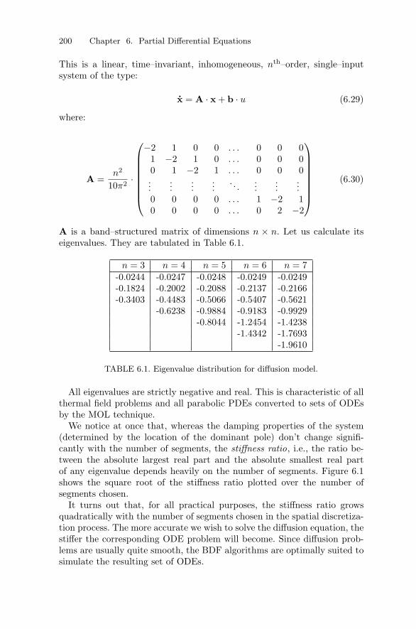
A is a band–structured matrix of dimensions n × n. Let us calculate itseigenvalues. They are tabulated in Table 6.1.
n = 3 n = 4 n = 5 n = 6 n = 7-0.0244 -0.0247 -0.0248 -0.0249 -0.0249-0.1824 -0.2002 -0.2088 -0.2137 -0.2166-0.3403 -0.4483 -0.5066 -0.5407 -0.5621
-0.6238 -0.9884 -0.9183 -0.9929-0.8044 -1.2454 -1.4238
-1.4342 -1.7693-1.9610
TABLE 6.1. Eigenvalue distribution for diffusion model.
All eigenvalues are strictly negative and real. This is characteristic of allthermal field problems and all parabolic PDEs converted to sets of ODEsby the MOL technique.
We notice at once that, whereas the damping properties of the system(determined by the location of the dominant pole) don’t change signifi-cantly with the number of segments, the stiffness ratio, i.e., the ratio be-tween the absolute largest real part and the absolute smallest real partof any eigenvalue depends heavily on the number of segments. Figure 6.1shows the square root of the stiffness ratio plotted over the number ofsegments chosen.
It turns out that, for all practical purposes, the stiffness ratio growsquadratically with the number of segments chosen in the spatial discretiza-tion process. The more accurate we wish to solve the diffusion equation, thestiffer the corresponding ODE problem will become. Since diffusion prob-lems are usually quite smooth, the BDF algorithms are optimally suited tosimulate the resulting set of ODEs.

6.3 Parabolic PDEs 201
10 15 20 25 30 35 40 45 5010
20
30
40
50
60
70
Stiffness Ratio of 1D Diffusion Problem
Number of Segments
√ Stiff
ness
Rat
io
FIGURE 6.1. Dependence of stiffness ratio on discretization.
We chose a PDE problem, the analytical solution of which is known. Ithappens to be:
uc(x, t) = exp(−t/10) · cos(π · x) (6.31)
Hence we can compare the analytical solution of the original PDE prob-lem with the equally analytical solution of the discretized ODE problemafter applying the MOL discretization.
The analytical solution of the discretized ODE problem is a little harderto come by. We can create a system description of the continuous–timeproblem:
x = A · x + b · u (6.32a)y = C · x + d · u (6.32b)
where C is an identity matrix of suitable dimensions, and d is a zero vectorusing MATLAB’s control system toolbox:
Sc = ss(A,b,C,d) (6.33)
This continuous–time system can then be converted to an equivalent discrete–time system:
xk+1 = F · xk + g · uk (6.34a)yk = H · xk + i · uk (6.34b)
using the statement:
Sd = c2d(Sc, h) (6.35)
from which the F–matrix and g–vector of the discrete state equations canbe extracted using the statement:

202 Chapter 6. Partial Differential Equations
[F,g] = ssdata(Sd) (6.36)
The discrete–time system can now be “simulated” by means of iteration ofthe discrete state equations. The solution of the discrete difference equation(ΔE) system is identical with that of the continuous ODE problem at thesampling points k ·h, where h is the step size (sampling rate) of the discreteproblem, except for the discretization of the input function. The discretesystem assumes that the input function u(t) is kept constant in betweensampling points.
Consequently, the step size, h, must be chosen small enough for the effectof the discretization of the input function to be negligible.
Let us look at the results of the experiment. The top left graph of Fig.6.2shows the solution of the PDE problem, uc, as a function of space andtime, whereas the top right graph shows the solution of the discretizedODE problem, ud, simulated using the approach discussed above. The twographs look identical by visual inspection. The bottom left graph of Fig.6.2displays the difference between the two functions, i.e.:
err = uc − ud (6.37)
and the bottom right graph of Fig.6.2 presents the maximum error, ermax,as a function of the number of segments used in the discretization. Themaximum error was computed using the MATLAB statement:
ermax = max(max(abs(err))); (6.38)
The step size, h, was chosen small enough so that a further reduction of hwould not visibly change the bottom right graph of Fig.6.2 any longer. Inthe given example, a step size of h = 0.001 had to be chosen to accomplishthis goal.
We have just come across a new type of error. The consistency errordescribes the difference between the original PDE problem that we wish tosolve, and the discretized ODE problem that we are actually solving.
Evidently, the consistency error cannot be overcome by either step–sizeor order control of the underlying ODE solver. Even the best ODE solvercan only approximate the analytical solution, ud, of the discretized ODEproblem, but never the true analytical solution, uc, of the original PDEproblem.
Is the consistency error a modeling error or a simulation error? The an-swer to this question depends on the point of view. If we use a modelingenvironment that allows us to describe the PDE problem directly, we areinclined to call this a simulation error. However, it is an error that is in-curred during the symbolic formulae manipulations that accompany thecompilation of the model, rather than at run time. On the other hand, ifwe use a lower–level modeling environment that forces us to convert the

6.3 Parabolic PDEs 203
1D Diffusion − Error
Number of Segments
Err
or
FIGURE 6.2. Solution of the 1D heat diffusion problem.
PDE manually into a set of ODEs, we would be more inclined to call thisa modeling error.
Can the consistency error be overcome by choosing a more accuratescheme for the computation of the spacial derivatives? Let us use a 5th–order accurate central difference scheme together with an equally 5th–orderaccurate biased difference scheme for the discretization points near the twoboundaries, hence:
u1 = exp(−t/10) (6.39a)
u2 =n2
120π2· (u6 − 6u5 + 14u4 − 4u3 − 15u2 + 10u1) (6.39b)
u3 =n2
120π2· (−u5 + 16u4 − 30u3 + 16u2 − u1) (6.39c)
u4 =n2
120π2· (−u6 + 16u5 − 30u4 + 16u3 − u2) (6.39d)
etc.nonumber (6.39e)
un−1 =n2
120π2· (−un+1 + 16un − 30un−1 + 16un−2 − un−3) (6.39f)
un =n2
120π2· (16un+1 − 31un + 16un−1 − un−2) (6.39g)
204 Chapter 6. Partial Differential Equations
un+1 =n2
60π2· (−15un+1 + 16un − un−1) (6.39h)
The bulk of the equations are formulated using 5th–order accurate cen-tral differences. Equation (6.39b) is specified using the 5th–order accuratebiased difference formula, whereas Eqs.(6.39g) and (6.39h) are derived bymaking use of the symmetry boundary condition.
Hence the resulting A–matrix takes the form:
A =n2
120π2·
⎛⎜⎜⎜⎜⎜⎜⎜⎜⎜⎜⎜⎝
−15 − 4 14 − 6 1 . . . 0 0 0 016 −30 16 − 1 0 . . . 0 0 0 0− 1 16 −30 16 − 1 . . . 0 0 0 0
0 − 1 16 −30 16 . . . 0 0 0 0
.
.
....
.
.
....
.
.
.. . .
.
.
....
.
.
....
0 0 0 0 0 . . . 16 −30 16 − 10 0 0 0 0 . . . − 1 16 −31 160 0 0 0 0 . . . 0 − 2 32 −30
⎞⎟⎟⎟⎟⎟⎟⎟⎟⎟⎟⎟⎠
(6.40)
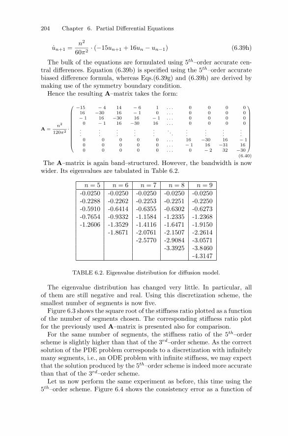
The A–matrix is again band–structured. However, the bandwidth is nowwider. Its eigenvalues are tabulated in Table 6.2.
n = 5 n = 6 n = 7 n = 8 n = 9-0.0250 -0.0250 -0.0250 -0.0250 -0.0250-0.2288 -0.2262 -0.2253 -0.2251 -0.2250-0.5910 -0.6414 -0.6355 -0.6302 -0.6273-0.7654 -0.9332 -1.1584 -1.2335 -1.2368-1.2606 -1.3529 -1.4116 -1.6471 -1.9150
-1.8671 -2.0761 -2.1507 -2.2614-2.5770 -2.9084 -3.0571
-3.3925 -3.8460-4.3147
TABLE 6.2. Eigenvalue distribution for diffusion model.
The eigenvalue distribution has changed very little. In particular, allof them are still negative and real. Using this discretization scheme, thesmallest number of segments is now five.
Figure 6.3 shows the square root of the stiffness ratio plotted as a functionof the number of segments chosen. The corresponding stiffness ratio plotfor the previously used A–matrix is presented also for comparison.
For the same number of segments, the stiffness ratio of the 5th–orderscheme is slightly higher than that of the 3rd–order scheme. As the correctsolution of the PDE problem corresponds to a discretization with infinitelymany segments, i.e., an ODE problem with infinite stiffness, we may expectthat the solution produced by the 5th–order scheme is indeed more accuratethan that of the 3rd–order scheme.
Let us now perform the same experiment as before, this time using the5th–order scheme. Figure 6.4 shows the consistency error as a function of

6.3 Parabolic PDEs 205
10 15 20 25 30 35 40 45 5010
20
30
40
50
60
70
80
5th−order
scheme
3rd−order
scheme
Stiffness Ratio of 1D Diffusion Problem
Number of Segments
√ Stiff
ness
Rat
io
FIGURE 6.3. Dependence of stiffness ratio on discretization.
the number of segments used in the discretization scheme. The results ofusing the 3rd–order accurate discretization scheme and those using the 5th–order accurate discretization scheme are superposed on the same graph.
0 10 20 30 40 50 60 70 80 90 1000
2
4
6
8x 10
−4
5th−order
scheme
3rd−order
scheme
1D Diffusion - Error
Number of Segments
Con
sist
ency
Err
or
FIGURE 6.4. Consistency error of the 1D heat diffusion problem.
The improvement achieved by the more accurate discretization schemeis quite dramatic. Yet, the “simulation” of the discretized problem is muchmore expensive in this case. We had to choose a smaller step size of h =0.0001 before the consistency error would no longer decrease by furtherreducing the step size.
206 Chapter 6. Partial Differential Equations
This observation is not overly surprising. Since the stiffness ratio forthe same number of segments has grown, yet the slowest eigenvalues havenot moved, the fastest eigenvalues are now much further to the left in thecomplex λ–plane. Hence we need to choose a smaller step size, h, in orderto operate within the accuracy region of the complex λ · h–plane of thenumerical simulation scheme.
This, unfortunately, is the biggest crux in the numerical solution ofparabolic PDE problems. If we double the number of segments, the num-ber of ODEs to be simulated doubles as well. However, since the stiffnessratio grows quadratically in the number of segments, the step size needsto decrease inverse quadratically in order to keep the accuracy the same inthe complex λ · h–plane. Hence doubling the number of segments forces usto quadruple the number of time steps. Hence the simulation effort growscubically in the number of segments.
Let us try another approach. You certainly remember the Richardsonextrapolation technique that we talked about in Chapter 3 of this text. Letus ascertain whether Richardson extrapolation may provide us with betteranswers to our approximation problem.
We can find four different third–order accurate approximations of ∂2u/∂x2:
∂2u
∂x2
∣∣∣∣P1
x=xi
(δx2) =ui+1 − ui + ui−1
δx2(6.41a)
∂2u
∂x2
∣∣∣∣P2
x=xi
(4δx2) =ui+2 − ui + ui−2
4δx2(6.41b)
∂2u
∂x2
∣∣∣∣P3
x=xi
(9δx2) =ui+3 − ui + ui−3
9δx2(6.41c)
∂2u
∂x2
∣∣∣∣P4
x=xi
(16δx2) =ui+4 − ui + ui−4
16δx2(6.41d)
These approximations differ only in the grid width δx used to obtain them.We can write:
∂2u
∂x2(η) =
∂2u
∂x2+ e1 · η + e2 · η2
2!+ e3 · η3
3!+ . . . (6.42)
where ∂2u/∂x2 is the true (yet unknown) value of the second spatial deriva-tive of u, whereas ∂2u(η)/∂x2 is the numerical value that we find when weapproximate the second spatial derivative using a grid width of η. Obvi-ously, this value contains an error. Equation (6.42) is a Taylor–Series inη around the (unknown) correct value. The ei variables are errors of theapproximation.
We truncate the Taylor Series after the cubic term, and write Eq.(6.42)down for the same values of the grid width that had been used in Eqs.(6.41a–d). We find:

6.3 Parabolic PDEs 207
∂2u
∂x2
P1
(δx2) ≈ ∂2u
∂x2+ e1 · δx2 +
e2
2!· δx4 +
e3
3!· δx6
∂2u
∂x2
P2
(4δx2) ≈ ∂2u
∂x2+ e1 · (4δx2) +
e2
2!· (4δx2)2 +
e3
3!· (4δx2)3
∂2u
∂x2
P3
(9δx2) ≈ ∂2u
∂x2+ e1 · (9δx2) +
e2
2!· (9δx2)2 +
e3
3!· (9δx2)3
∂2u
∂x2
P4
(16δx2) ≈ ∂2u
∂x2+ e1 · (16δx2) +
e2
2!· (16δx2)2 +
e3
3!· (16δx2)3
(6.43)
or in a matrix notation:
⎛⎜⎜⎜⎜⎝
∂2u∂x2
P1
∂2u∂x2
P2
∂2u∂x2
P3
∂2u∂x2
P4
⎞⎟⎟⎟⎟⎠ ≈
⎛⎜⎜⎝
(δx2)0 (δx2)1 (δx2)2 (δx2)3
(4δx2)0 (4δx2)1 (4δx2)2 (4δx2)3
(9δx2)0 (9δx2)1 (9δx2)2 (9δx2)3
(16δx2)0 (16δx2)1 (16δx2)2 (16δx2)3
⎞⎟⎟⎠ ·
⎛⎜⎜⎝
∂2u∂x2
e1
e2/2e3/6
⎞⎟⎟⎠(6.44)
By inverting the Van–der–Monde matrix, we can solve for the unknown∂2u/∂x2 and the three error variables. Since we aren’t interested in theerrors, we only look at the first row of the inverted Van–der–Monde matrix.It turns out that the values in this row don’t depend at all on the grid widthδx. We find:
∂2u
∂x2≈ ( 56
35 − 2835
835 − 1
35
) ·⎛⎜⎜⎜⎜⎝
∂2u∂x2
P1
∂2u∂x2
P2
∂2u∂x2
P3
∂2u∂x2
P4
⎞⎟⎟⎟⎟⎠ (6.45)
We can plug Eqs.(6.41) into Eq.(6.45), and find:
∂2u
∂x2
∣∣∣∣x=xi
≈ 15040δx2
(−9ui+4 + 128ui+3 − 1008ui+2 + 8064ui+1
− 14350ui + 8064ui−1 − 1008ui−2 + 128ui−3 − 9ui−4) (6.46)
which is exactly the central difference formula of order 9. Once again,the Richardson extrapolation has raised the approximation accuracy to thehighest possible order.
Let us now look at a slightly different problem:
208 Chapter 6. Partial Differential Equations
∂u
∂t= 4
∂2u
∂x2; x ∈ [0, 1] ; t ∈ [0,∞) (6.47a)
u(x, t = 0) = 20 sin(π
2x)
+ 300 (6.47b)
u(x = 0, t) = 20 sin( π
12t)
+ 300 (6.47c)
∂u
∂x(x = 1, t) = 0 (6.47d)
We again solve a one–dimensional heat equation, but with a different timeconstant, and different initial and boundary conditions.
This time around, we don’t know the analytical solution, hence we cannotcompute the consistency error explicitly. What do we do? Similarly to thestep–size control algorithms discussed in the previous chapters, we need anestimator of the spatial discretization error.
All numerical algorithms should have a second algorithm built in to themthat reasons about the sanity of the first algorithm and starts screaming ifit thinks that something is going awry. Without such a sanity check, numer-ical algorithms are never safe. It is precisely the availability of such alarmsystems that constitutes one of the major distinctions between productioncodes and experimental codes.
We propose to compute all spatial derivatives twice, once with the gridsize δx, and once with the grid size 2δx using central differences.
∂2u
∂x2
∣∣∣∣P1
x=xi
(δx2) =ui+1 − ui + ui−1
δx2(6.48a)
∂2u
∂x2
∣∣∣∣P2
x=xi
(4δx2) =ui+2 − ui + ui−2
4δx2(6.48b)
(6.48c)
The two approximations form two separate partial derivative vectors, uP1xx
and uP2xx . Using these approximations, we can formulate a spatial error
estimate:
εrel =|uP1
xx − uP2xx |
max(|uP1xx |, |uP2
xx |, δ)(6.49)
where δ is a fudge factor, e.g., δ = 10−10.If the estimated spatial discretization error is too big, we must either
choose a more narrow grid, or alternatively, we must increase the approxi-mation order of the spatial derivatives.
Is it wasteful to compute the entire vector of spatial derivatives twice?This question must clearly be answered in the negative. The two predictorscan be used in a Richardson corrector step:

6.3 Parabolic PDEs 209
uCxx =
43· uP1
xx − 13· uP2
xx (6.50)
This is equivalent to having raised the approximation order of the spatialderivatives from three to five. However, by writing the 5th–order accuratespatial derivative formula in this way, we get an error estimator essentiallyfor free.
Since the problem is stiff, a BDF formula may be appropriate for itsintegration. As we wish to obtain a global accuracy of 1%, we decided tosimulate the system using BDF3. We chose nseg = 50 in order to receivesufficiently many output points in space, and simulated across 10 secondsin time. The simulation results are shown in Fig.6.5.
0
0.2
0.4
0.6
0.8
1
0
2
4
6
8
10300
305
310
315
320
Space
1D Diffusion
Time
Solu
tion
FIGURE 6.5. Solution of heat diffusion problem.
Figure 6.6 shows a slice through the solution at x = 1.0.Unfortunately, the solution exhibits a fast transient precisely during the
start–up period. The problem isn’t truly stiff until the fast transients havedied out. Initially, the solution is heavily controlled by accuracy require-ments beside from the numerical stability constraints.
Assuming a fixed step size to be used throughout the solution, we re-peated the simulation thrice, once using order buildup, i.e., a BDF starter,once using an RK3 starter, and once using an IEX3 starter. Figure 6.7shows the step size required to achieve a desired level of accuracy usingthese three start–up algorithms.

210 Chapter 6. Partial Differential Equations
0 1 2 3 4 5 6 7 8 9 10300
305
310
315
320
325
1D Diffusion
Time
Solu
tion
FIGURE 6.6. Solution of heat diffusion problem.
10−3
10−2
10−1
10−10
10−5
100
BDF
RK3
IEX3
Accuracy vs. Cost
Step size
Rel
ativ
eer
ror
FIGURE 6.7. Accuracy vs. cost for different start–up algorithms.
Overall, the accuracy of the simulation seems to be quite a bit betterthan the 3rd–order algorithm would have made us believe. In addition,the effect of the start–up algorithm on the simulation accuracy is quitedramatic. For small step sizes, the RK3 starter seems to work much betterthan the BDF starter. However, at h = 0.005, the numerical stability is lost,and the overall accuracy of the simulation degrades rapidly, in spite of thefact that the RK3 algorithm is only being used during the first two stepsof the simulation. Of course, an RK starter implemented in a productioncode would be expected to proceed with a smaller step size than during theremainder of the simulation, but we did not want to make use of any type ofstep–size control in this experiment, as this would make an interpretationof the obtained results much more difficult.
The IEX3 starter, implemented using BDF1 steps internally, performssimilarly to the RK3 starter for small step sizes, but without being plaguedby the numerical stability problems of the RK3 starter for larger step sizes.
We also tried a BI4/50.45 starter. It didn’t work well at all in this ap-plication. The reason is the following. The backward RK semi–step is nu-merically highly unstable. It is only stabilized by the Newton iteration. Inthe given application, we ran into roundoff error problems. The unstable
6.4 Hyperbolic PDEs 211
semi–step produced numbers so big that the Newton iteration could notstabilize them any longer due to roundoff.
Parabolic PDE problems discretized using the MOL approach alwaysturn into very stiff ODE systems. The more accurate we wish to simulate,the stiffer the problem becomes. Yet, decent stiff system solvers, such asDASSL [6.1], are usually quite capable of dealing with such problemseffectively and efficiently.
6.4 Hyperbolic PDEs
Let us now analyze the second class of PDE problems, the hyperbolic PDEs.The simplest specimen of this class of problems is the wave equation orlinear conservation law :
∂2u
∂t2= c2 · ∂2u
∂x2(6.51)
We can easily transform this second–order PDE in time into two first orderPDEs in time:
∂u
∂t= v (6.52a)
∂v
∂t= c2 · ∂2u
∂x2(6.52b)
At this point, we can replace the spatial derivatives again by finite differenceapproximations, and we seem to be in business.
Equations (6.53a–e) constitute a complete specification of such a model.
∂2u
∂t2=
∂2u
∂x2; x ∈ [0, 1] ; t ∈ [0,∞) (6.53a)
u(x, t = 0) = sin(π
2x)
(6.53b)
∂u
∂t(x, t = 0) = 0.0 (6.53c)
u(x = 0, t) = 0.0 (6.53d)∂u
∂x(x = 1, t) = 0.0 (6.53e)
Equation (6.53a) is the one–dimensional wave equation, Eqs.(6.53b–c) con-stitute its two initial conditions, and Eqs.(6.53d–e) describe its two bound-ary conditions.
Let us simulate this problem using the MOL approach. We decide to splitthe spatial axis into n segments of width δx = 1/n. If we work with the

212 Chapter 6. Partial Differential Equations
central difference formula of Eq.(6.7), and using the symmetry boundarycondition approach at the right end of the interval, we obtain the followingset of ODEs:
u1 = 0.0 (6.54a)u2 = v2 (6.54b)etc.un+1 = vn+1 (6.54c)v1 = 0.0 (6.54d)
v2 = n2 (u3 − 2u2 + u1) (6.54e)
v3 = n2 (u4 − 2u3 + u2) (6.54f)etc.
vn = n2 (un+1 − 2un + un−1) (6.54g)
vn+1 = 2n2 (un − un+1) (6.54h)
with the initial conditions:
u2(0) = sin( π
2n
)(6.55a)
u3(0) = sin(π
n
)(6.55b)
u4(0) = sin(
3π
2n
)(6.55c)
etc.
un(0) = sin(
(n − 1)π2n
)(6.55d)
un+1(0) = sin(π
2
)(6.55e)
v2(0) = 0.0 (6.55f)etc.vn+1(0) = 0.0 (6.55g)
This is a linear, time–invariant, inhomogeneous, (2n)th–order, single–inputsystem of the type specified in Eq.(6.29), where:
A =(
0(n) I(n)
A21 0(n)
)(6.56)
with:

6.4 Hyperbolic PDEs 213
A21 = n2
⎛⎜⎜⎜⎜⎜⎜⎜⎝
−2 1 0 0 . . . 0 0 01 −2 1 0 . . . 0 0 00 1 −2 1 . . . 0 0 0...
......
.... . .
......
...0 0 0 0 . . . 1 −2 10 0 0 0 . . . 0 2 −2
⎞⎟⎟⎟⎟⎟⎟⎟⎠
(6.57)
A is a band–structured matrix of dimensions 2n× 2n with two separatenon–zero bands. Let us calculate its eigenvalues. They are tabulated inTable 6.3.
n = 3 n = 4 n = 5 n = 6±1.5529j ±1.5607j ±1.5643j ±1.5663j±4.2426j ±4.4446j ±4.5399j ±4.5922j±5.7956j ±6.6518j ±7.0711j ±7.3051j
±7.8463j ±8.9101j ±9.5202j±9.8769j ±11.0866j
±11.8973j
TABLE 6.3. Eigenvalue distribution of linear conservation law.
All eigenvalues are strictly imaginary. All hyperbolic PDEs converted tosets of ODEs using the MOL technique show complex eigenvalues. Many ofthem have their eigenvalues spread up and down fairly close to the imagi-nary axis. The linear conservation law has all its eigenvalues exactly on theimaginary axis.
Figure 6.8 shows the frequency ratio, i.e., the ratio between the absolutelargest and the absolute smallest imaginary parts of any eigenvalues plottedover the number of segments used in the discretization.
10 15 20 25 30 35 40 45 5010
20
30
40
50
60
70
Frequency Ratio of 1D Linear Conservation Law
Number of Segments
Freq
uenc
yR
atio
FIGURE 6.8. Frequency ratio of the 1D linear conservation law.
Evidently, the frequency ratio of the 1D linear conservation law growslinearly with the number of segments used in the discretization.

214 Chapter 6. Partial Differential Equations
The numerical challenges are quite different from those in the paraboliccase. The conservation law does not lead to a stiff set of ODEs. No “fasttransients” appear that die out after some time, and consequently, thestep size in the numerical integration must be kept small to account forall the eigenvalues of the discretized problem. The more narrow the gridwidth is chosen, the smaller the time steps will have to be in order to keepall eigenvalues within the asymptotic region of the numerical integrationalgorithm. Luckily, the spreading of the eigenvalues grows only linearlywith the number of segments chosen.
We have seen that PDEs pose a new kind of challenge. In the case ofODE solutions, we only worried about stability and accuracy. In the caseof PDE solution, we must concern ourselves with stability , accuracy , andconsistency .
Definition: “A discretization scheme is called consistent if theanalytical solution of the discretized problem smoothly approachesthe analytical solution of the original continuous problem as thegrid width is being reduced to smaller and smaller values.”
The consistency error is thus the deviation of the analytical solution of thediscretized problem from the analytical solution of the continuous problem,whereas the accuracy error is the deviation of the numerical solution of thediscretized problem from the analytical solution of the discretized problem.1
The example of Eqs.(6.53a–e) is so simple that an analytical solution ofthe continuous (field) problem can be given. It is:
u(x, t) =12
sin(π
2(x − t)
)+
12
sin(π
2(x + t)
)(6.58)
Since the discretized problem is linear with constant input, we can use themethod described in Hw.[H4.8] to derive its analytical solution. Thus, wecan go after the consistency error directly.
Figure 6.9 shows in its top left graph the analytical solution of the orig-inal PDE problem, in its top right graph the analytical solution of thediscretized ODE problem. The two solutions look identical when comparedby the naked eye. The bottom left curve shows the difference between thetop two curves.
Since the input function is zero, the solution of the discretized ODE prob-lem is independent of the chosen step size, h, in time. The discretization in
1Traditionally, the numerical PDE literature talks about the three facets: stability,consistency, and convergence. It is then customary to prove that any two of the threeimply the third one, i.e., it is sufficient to look at any selection of two of the three [6.13].However, that way of reasoning is more conducive to fully discretized (finite differenceor finite element) schemes, where the step size in time, h, is locked in a fixed relationshipwith the grid width in space, δx. Consequently, h and δx approach zero simultaneously.In the context of the MOL methodology, our approach may be more appealing.

6.4 Hyperbolic PDEs 215
Consistency Error
Number of Segments
Err
or
FIGURE 6.9. Analytical solutions of the 1D wave equation.
time serves here only for the purpose of generating sufficiently many outputpoints. Hence the curve shown in the bottom left graph is the true consis-tency error. The only potential sources of numerical pollution could be dueto roundoff and accumulation, but these are insignificant in magnitude incomparison with the analytical consistency error.
The bottom right graph shows the consistency error plotted against thenumber of segments chosen for the spatial discretization. The consistencyerror is here much larger than in the previous parabolic PDE examples. Ifwe wish to obtain simulation results with a numerical accuracy of 1%, theconsistency error itself ought to be at least one order of magnitude smaller.This means we should choose at least 40 segments for this simulation.
Just like in the case of the parabolic PDE problems, let us discuss whathappens when we choose a higher–order discretization in space. Let us tryfirst with 5th–order central differences.
Figure 6.10 shows the frequency ratio plotted against the number ofsegments chosen in the spatial discretization scheme. The frequency ratioof the 3rd–order scheme is plotted on the same graph for comparison.
The frequency ratio of the more accurate 5th–order scheme is consistentlyhigher than that of the less accurate 3rd–order scheme for the same num-ber of segments. Since the true PDE solution, corresponding to the solutionwith infinitely many infinitely dense discretization lines, has a frequencyratio that is infinitely large, we suspect that choosing a higher–order dis-cretization scheme may indeed help with the reduction of the consistency

216 Chapter 6. Partial Differential Equations
10 15 20 25 30 35 40 45 5010
20
30
40
50
60
70
80
5th−order
scheme
3rd−order
scheme
Frequency Ratio of 1D Linear Conservation Law
Number of Segments
Freq
uenc
yR
atio
FIGURE 6.10. Frequency ratio of the 1D wave equation.
error.Figure 6.11 shows the consistency error plotted over the number of seg-
ments used in the discretization. The improvement is quite dramatic. Theconsistency error has been reduced by at least two orders of magnitude.
10 15 20 25 30 35 40 45 500
0.2
0.4
0.6
0.8
1x 10
−4 1D Linear Conservation Law
Number of Segments
Con
sist
ency
Err
or
FIGURE 6.11. Consistency error of the 1D wave equation.
In a true simulation experiment, the 5th–order spatial discretizationscheme should be implemented using the Richardson predictor–correctortechnique presented earlier in this chapter.
Let us compute the cost–versus–accuracy plot for the above problem,comparing the various third–order algorithms to each other that we mean-while know. We shall use 50 segments for the spatial discretization togetherwith 5th–order central differences, in order to keep the consistency errorsufficiently small, so that it won’t affect the simulation results.
We computed the global accuracy of seven algorithms for simulating thediscretized wave equation across 10 seconds of simulated time using a fixedstep size of h, namely: RK3, IEX3, BI3, AB3, ABM3, AM3, and BDF3. Wechose the step sizes: h = 0.1, h = 0.05, h = 0.02, h = 0.01, h = 0.005, h =0.002, and h = 0.001 corresponding to 100, 200, 500, 1000, 2000, 5000, and10000 steps, respectively. The results are tabulated in Table 6.4.

6.4 Hyperbolic PDEs 217
h RK3 IEX3 BI30.1 unstable 0.6782e-4 0.4947e-60.05 unstable 0.8668e-5 0.2895e-70.02 unstable 0.5611e-6 0.1324e-80.01 0.7034e-7 0.7029e-7 0.2070e-80.005 0.8954e-8 0.8791e-8 0.2116e-80.002 0.2219e-8 0.2145e-8 0.2120e-80.001 0.2127e-8 0.2119e-8 0.2120e-8
h AB3 ABM3 AM3 BDF30.1 unstable unstable unstable garbage0.05 unstable unstable unstable garbage0.02 unstable unstable unstable garbage0.01 unstable 0.6996e-7 unstable garbage0.005 0.7906e-7 0.8772e-8 0.8783e-8 0.9469e-20.002 0.5427e-8 0.2156e-8 0.2149e-8 0.1742e-60.001 0.2239e-8 0.2120e-8 0.2120e-8 0.4363e-7
TABLE 6.4. Comparison of accuracy of integration algorithms.
Using a step size of h = 0.001, all seven integration algorithms simulatethe problem successfully. In fact, all of them with the exception of BDF3are down to the level of the consistency error.
As the step size becomes smaller, the higher–order terms in the Taylor–series expansion become less and less important. For sufficiently small stepsizes, all integration algorithms behave either like forward or backwardEuler.
BDF3 performs a little poorer than the other algorithms, because itserror coefficient is considerably larger than those of its competitors. BDFalgorithms perform generally somewhat poor in terms of accuracy in com-parison with their peers of equal order. The BDF algorithms had beenknown before they were made popular by Bill Gear in the early seventies[6.9]. However, they were considered “garbage algorithms” due to their pooraccuracy properties.
It turns out that the problem is kind of “stiff,” although it does not meetmost of John Lambert’s definitions of stiffness [6.11]. The problem is “stiff”in the sense that all the algorithms with stability domains looping into theleft–half plane are unable to produce solutions with the desired accuracyof 1.0%, since they are numerically unstable when a step size is used thatwould produce the desired accuracy otherwise. BDF3 doesn’t suffer thesame fate, but it eventually succumbs to error accumulation problems. Asthe step sizes grow too big, the computations become so inaccurate thatthe simulation error exceeds the simulation output in magnitude. Hence

218 Chapter 6. Partial Differential Equations
BDF3 starts accumulating numerical garbage.Only IEX3 and BI3 are capable of solving the problem successfully for
large step sizes. Between the two, BI3 seems to work a little better, whichis no big surprise. Being an F–stable algorithm, BI3 is earmarked for thesetypes of applications.
Figure 6.12 presents the same results graphically in a cost vs. accuracyplot.
10−9
10−8
10−7
10−6
10−5
10−4
102
103
104
105
106
RK3
IEX3
BI3
10−9
10−8
10−7
10−6
10−5
10−4
102
103
104
105
106
AB3,ABM3
AM3 BDF3
1D Linear Conservation Law - Error
Simulation accuracy
Simulation accuracy
#fu
ncti
onev
alua
tion
s#
func
tion
eval
uati
ons
FIGURE 6.12. Cost vs. accuracy of the 1D wave equation.
These results are somewhat deceiving, since they do not take into accountthe effort spent in computing inverse Hessians. This decision was taken onpurpose, since the number of function evaluations is the only objectivemeasure available that depends on the algorithm alone, rather than onimplementational details of the production code, as different codes vary alot in how often and how accurately they compute inverse Hessians.
Of course, since the given problem is linear and since we don’t varythe step size ever, it would suffice to compute one inverse Hessian at thebeginning of the simulation. Yet, this fact is peculiar to the specific problemat hand. For nonlinear problems, the explicit algorithms, i.e., RK3, AB3,and ABM3, may be at least as attractive as BI3.
We would still argue in favor of the BI algorithms for these types ofapplications, not because of their superior cost–per–accuracy properties,but because of their better robustness characteristics. Using BI3, we can

6.5 Shock Waves 219
obtain a decent answer using any step size that we may try without havingthe algorithm blow up on us, and we get a meaningful accuracy in eachand every case.
We could have included also GE3 in the comparison of this section.Since the problem to be solved is a linear conservation law, the stand–alone versions of the explicit Godunov schemes would have been excellentlysuited for the task at hand. However, we decided against doing so, becausethe comparison would have been quite unfair. All of the techniques com-pared against each other in this section are general–purpose numerical ODEsolvers, whereas the stand–alone versions of the GE algorithms are limitedto dealing with linear conservation laws only.
6.5 Shock Waves
Let us now study a more involved hyperbolic PDE problem. A thin tube oflength 1 m is initially pressurized at pB = 1.1 atm. The tube is located atsea level, i.e., the surrounding atmosphere has a pressure of p0 = 1.0 atm =760.0 Torr = 1.0132 · 105 N m−2. The current temperature is T = 300.0 K.At time zero, the tube is opened at one of its two ends. We wish to determinethe pressure at various places inside the tube as functions of time.1
As the tube is opened, air rushes out of the tube, and a rarefaction waveenters the pipe. Had the initial pressure inside the pipe been smaller thanthe outside pressure, air would have rushed in, and a compression wavewould have formed.
The problem can be mathematically described by a set of first–orderhyperbolic PDEs:
∂ρ
∂t= −v · ∂ρ
∂x− ρ · ∂v
∂x(6.59a)
∂v
∂t= −v · ∂v
∂x− a
ρ(6.59b)
∂p
∂t= −v · a − γ · p · ∂v
∂x(6.59c)
a =∂p
∂x+
∂q
∂x+ f (6.59d)
q =
{β · δx2 · ρ · ( ∂v
∂x
)2; ∂v
∂x < 0.00.0 ; ∂v
∂x ≥ 0.0(6.59e)
f =α · ρ · v · |v|
δx(6.59f)
1The problem can be found in a slightly modified form in the FORSIM–VI manual[6.4]. It is being reused here with the explicit permission by the author.

220 Chapter 6. Partial Differential Equations
where ρ(x, t) denotes the gas density inside the tube at position x and timet, v(x, t) denotes the gas velocity , and p(x, t) denotes the gas pressure.The quantity a was pulled out into a separate algebraic equation, since thesame quantity is used in two places within the model. The two quantitiescomputed in Eqs.(6.59e–f) are artificial, as their dependence on δx shows.Clearly, δx is not a physical quantity, but is introduced only in the processof converting the (small) set of PDEs into a (large) set of ODEs. q denotesthe pseudo viscous pressure, and f denotes the frictional resistance. Theywere introduced by Richtmyer and Morton [6.14] in order to smoothenout numerical problems with the solution. We shall discuss this issue indue course. γ is the ratio of specific heat constants, a non–dimensionalconstant with a value of γ = cp/cv = 1.4. α and β are non–dimensionalnumerical fudge factors. We shall initially assign the following values tothem: α = β = 0.1. The “ideal” (i.e., undamped) problem has α = β = 0.0.
Introduction of the two dissipative terms is not a bad idea, since the“ideal” solution does not represent a physical phenomenon in any truesense. Phenomena without any sort of dissipation belong allegedly in theworld that we may enter after we die. They certainly don’t form any partof this universe.
The initial conditions are:
ρ(x, t = 0.0) = ρB (6.60a)v(x, t = 0.0) = 0.0 (6.60b)p(x, t = 0.0) = pB (6.60c)
where ρB is determined by the equation of state for ideal gases (cf. Chap-ter 9 of the companion book Continuous System Modeling [6.5]):
ρB =pB · Mair
R · T (6.61)
where T = 300.0 is the absolute temperature (measured in Kelvin), R =8.314 J K−1 mole−1 is the gas constant, and Mair = 28.96 g mole−1 is theaverage molar mass of air.1 The boundary conditions are:
v(x = 0.0, t) = 0.0 (6.62a)ρ(x = 1.0, t) = ρ0 (6.62b){
v(x = 1.0, t) = −√
2(p0−p(x=1.0,t)ρ(x=1.0,t) ; v(x = 1.0, t) < 0.0
p(x = 1.0, t) = p0 ; v(x = 1.0, t) ≥ 0.0(6.62c)
1Air consists roughly to 78% of nitrogen (N2) with a molar mass of 28 g mole−1, to21% of oxygen (O2) with a molar mass of 32 g mole−1, and to 1% of argon (Ar) with amolar mass of 40 g mole−1.

6.5 Shock Waves 221
As proposed in [6.4], we converted all spatial derivatives by means ofsecond–order accurate central differences using the formula:
∂u
∂x
∣∣∣∣x=xi
≈ 12δx
· (ui+1 − ui−1) (6.63)
except near the boundaries, where we used second–order accurate biasedformulae:
∂u
∂x(x = x1, t) ≈ 1
2δx·(−u3 + 4u2 − 3u1) (6.64a)
∂u
∂x(x = xn+1, t) ≈ 1
2δx·(3un+1 − 4un + un−1) (6.64b)
where u can stand for either ρ, v, p, or q.In order to keep the consistency error small, we chose 50 segments for
each of the three PDEs. We created a MATLAB function:
ux = partial(u, δx, bc, bctype) (6.65)
which implements the above set of formulae with correction terms in thecase of a symmetry boundary condition. The variable bc indicates whetherthe boundary condition is applied at the left end, bc = −1, or at the rightend, bc = +1. The variable bctype specifies the type of boundary condition.bctype = 0 indicates a symmetry boundary condition. bctype = 1 denotesa function value condition.
In the case of a symmetry boundary condition, the central formulae areused all the way to the boundary while folding the values that are outsidethe domain back into the domain, as explained earlier.
The correction formulae are:
∂u
∂x(x = x1, t) ≈ 0.0 (6.66)
for a symmetry boundary condition at the left end, and:
∂u
∂x(x = xn+1, t) ≈ 0.0 (6.67)
for a symmetry boundary condition at the right end.The state–space model itself has been encoded in another MATLAB
function:
function [xdot] = st eq(x, t)%% State − space model of shock − tube problem%n = round(length(x)/3);n1 = n + 1;δx = 1/n;

222 Chapter 6. Partial Differential Equations
%% Constants%
R = 8.314;%% Physical parameters
%
Temp = 300;Mair = 0.02896;p0 = 1.0132e5;ρ0 = p0 ∗ Mair/(R ∗ Temp);
γ = 1.4;%% Fudge factors%global α β%% Unpack individual state vectors from total state vector%ρ = [ x(1 : n) ; ρ0 ];v = [ 0 ; x(n1 : 2 ∗ n) ];p = x(n1 + n : n1 + 2 ∗ n);%% Calculate nonlinear boundary condition%if v(n1) < 0,
v(n1) = −sqrt(max([2 ∗ (p0 − p(n1))/ρ(n1), 0]));else
p(n1) = p0;end%
% Calculate spatial derivatives%ρx = partial(ρ, δx, +1, +1);vx = partial(v, δx,−1, +1);px = partial(p, δx, +1, +1);%% Calculate algebraic quantities%f = α ∗ (ρ . ∗ v . ∗ abs(v))/δx;q = zeros(n1, 1);for i = 1 : n1,
if vx(i) < 0,q(i) = β ∗ (δx2) ∗ ρ(i) ∗ (vx(i)2);
end,endqx = partial(q, δx,−1, +1);a = px + qx + f ;%% Calculate temporal derivatives%ρt = −(v . ∗ ρx) − (ρ . ∗ vx);vt = −(v . ∗ vx) − (a ./ ρ);
6.5 Shock Waves 223
pt = −(v . ∗ a) − γ ∗ (p . ∗ vx);%% Pack individual state derivatives into total state derivative vector%xdot = [ ρt(1 : n) ; vt(2 : n1) ; pt ];
return
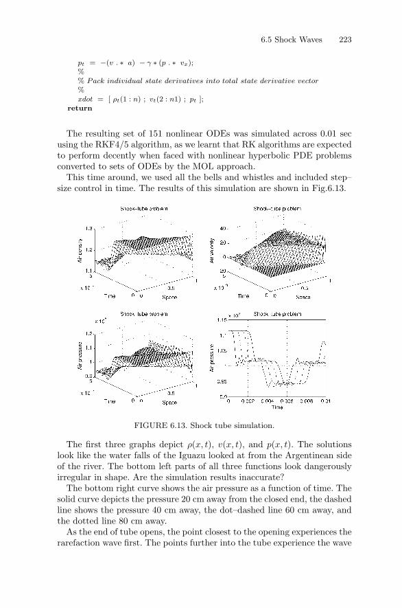
The resulting set of 151 nonlinear ODEs was simulated across 0.01 secusing the RKF4/5 algorithm, as we learnt that RK algorithms are expectedto perform decently when faced with nonlinear hyperbolic PDE problemsconverted to sets of ODEs by the MOL approach.
This time around, we used all the bells and whistles and included step–size control in time. The results of this simulation are shown in Fig.6.13.
Shock−tube problem
Time
Air p
ressure
FIGURE 6.13. Shock tube simulation.
The first three graphs depict ρ(x, t), v(x, t), and p(x, t). The solutionslook like the water falls of the Iguazu looked at from the Argentinean sideof the river. The bottom left parts of all three functions look dangerouslyirregular in shape. Are the simulation results inaccurate?
The bottom right curve shows the air pressure as a function of time. Thesolid curve depicts the pressure 20 cm away from the closed end, the dashedline shows the pressure 40 cm away, the dot–dashed line 60 cm away, andthe dotted line 80 cm away.
As the end of tube opens, the point closest to the opening experiences therarefaction wave first. The points further into the tube experience the wave

224 Chapter 6. Partial Differential Equations
later. From Fig.6.13, it can be concluded that the wave travels through thetube with a constant wave–front velocity of roughly 35 cm per 0.001 sec,or 350.0 m sec−1. This is the correct value of the velocity of sound at sealevel and at a temperature of T = 300 K. Thus, our simulation seems tobe working fine. (There is nothing more healthy in simulation of physicalsystems than a little reality check once in a while!)
As the rarefaction wave reaches the closed end of the tube, the inertiaof the flowing air creates a vacuum. The air flows further, but cannot bereplaced by more air from the left. Consequently, the air pressure now sinksbelow that of the outside air.
As the vacuum reaches the open end of the tube, a new wave is created,this time a compression wave, that races back into the tube.
We ended the simulation at t = 0.01 sec, since shortly thereafter, theRunge–Kutta algorithm would finally give up on us, and die with an errormessage.
How accurate are these simulation results? To answer this question, werepeated the simulation with 100 segments. The simulated air pressure atthe center of the tube, x = 50 cm, is shown in Fig.6.14. For comparison, theresults of the 50–segment simulation are superposed on the same graph. Asthe model itself depends explicitly on the grid width, we set α = β = 0.0for this experiment. In this way, the explicit (artificial) dependence of themodel on the grid width is eliminated.
0 0.001 0.002 0.003 0.004 0.005 0.006 0.007 0.008 0.009 0.010.9
0.95
1
1.05
1.1
1.15x 10
5
100
50
Shock-tube problem
Time
Air
pres
sure
FIGURE 6.14. Consistency error for shock tube simulation.
The simulation results are visibly different. Moreover, the differencesseem to grow over time. Is this a consistency error, or simply the result ofan inaccurate simulation?
To answer this question, we repeated the same experiment, this time us-ing a different integration algorithm. The F–stable Backinterpolation tech-nique is supposed to work at least as well as the RK algorithm.
The simulation results are indistinguishable by naked eye. Whereas thelargest relative distance between the air pressure with 50 and 100 segments:

6.5 Shock Waves 225
err =max(max(abs(p100 − p50)))
max([‖p100‖, ‖p50‖]) (6.68)
is err = 7.5726e − 4, the largest relative distance between the air pressurewith 50 segments comparing the two different integration algorithms iserr = 1.2374e − 7, and with 100 segments, it is err = 6.3448e − 7.
Hence the simulation error is smaller than the consistency error by threeorders of magnitude. Evidently, we are not faced with a simulation problemat all, but rather with a modeling problem. The simulation is as accurateas can be expected.
The BI4 algorithm is considerably less efficient than the RKF4/5 algo-rithm in simulating this problem. Its inefficiency is not caused by the stepsize. In fact, the step–size controlled BI4 algorithm can make use of stepsizes that are quite a bit larger than those used by RKF4/5. The ineffi-ciency is caused by the computation of the Jacobians and of the inverseHessians.
Since the problem is nonlinear, the Jacobians need to be numericallyestimated, using an algorithm such as:
function [J ] = jacobian(x, t)%% Jacobian of shock − tube problem%n = length(x);J = zeros(n, n);xdref = st eq(x, t);for i = 1 : n,
xnew = x;if abs(x(i)) < 1.0e − 6,
xnew(i) = 0.05;else
xnew(i) = 1.05 ∗ x(i);end,xdnew = st eq(x, t);J(:, i) = (xdnew − xdref )/(xnew(i) − x(i));
endreturn
Thus, every single Jacobian, which is being computed once per inte-gration step, requires 152 additional function evaluations in the case of a50–segment simulation, and 302 additional function evaluations in the caseof a 100–segment simulation. No wonder that production codes of implicitODE solvers are frugal in the frequency of Jacobian evaluations.
The Hessian is of the same size as the Jacobian:
H = I(n) + J · h +12!
· (J · h)2 +13!
· (J · h)3 +14!
· (J · h)4 (6.69)
where h = −h/2 is the step size of the right half–step of the BI4 algorithm.

226 Chapter 6. Partial Differential Equations
The Hessian is used in a Gauss elimination step once per iteration step:
while err2 > 0.1 ∗ tol,
[xright4, xright5] = rkf45 step(xnew, tnew,−h/2);nfct = nfct + 6;xnew = xnew − H\(xright4 − xleft4);err2 = norm(xright4 − xleft4, ′inf′)/max([norm(xleft4),norm(xright4), tol]);
end
The computational burden of these algorithms is atrocious. We shall haveto do something about the size of these matrices. This problem shall betackled in the next chapter of this book.
What can we do to reduce the consistency error? From our previousobservation, we know the answer to this question. If we increase the ap-proximation order of the spatial derivatives by two, the consistency erroris expected to decrease by two orders of magnitude.
We modified the partial function to use fourth–order accurate centraldifferences instead of the previously used second–order accurate centraldifferences. To this end, the following formulae were now coded into thepartial function:
∂u
∂x
∣∣∣∣x=xi
≈ 112δx
· (−ui+2 + 8ui+1 − 8ui−1 + ui−2) (6.70)
except near the boundaries, where we used fourth–order accurate biasedformulae:
∂u
∂x(x = x1, t) ≈ 1
12δx·(−3u5 + 16u4 − 36u3 + 48u2 − 25u1) (6.71a)
∂u
∂x(x = x2, t) ≈ 1
12δx·(u5 − 6u4 + 18u3 − 10u2 − 3u1) (6.71b)
∂u
∂x(x = xn, t) ≈ 1
12δx·(3un+1 + 10un − 18un−1 + 6un−2 − un−3)
(6.71c)∂u
∂x(x = xn+1, t) ≈ 1
12δx·(25un+1 − 48 ∗ un + 36un−1 − 16un−2
+ 3un−3) (6.71d)
In the case of a symmetry boundary condition, the central formulae areused all the way to the boundary while folding the values that are outsidethe domain back into the domain, as explained earlier.
The correction formulae are:

6.5 Shock Waves 227
∂u
∂x(x = x1, t) ≈ 0.0 (6.72a)
∂u
∂x(x = x2, t) ≈ 1
12δx· (−u4 + 8u3 + u2 − 8u1) (6.72b)
(6.72c)
for a symmetry boundary condition at the left end, and:
∂u
∂x(x = xn, t) ≈ 1
12δx· (8un+1 − un − 8un−1 + un−2) (6.73a)
∂u
∂x(x = xn+1, t) ≈ 0.0 (6.73b)
for a symmetry boundary condition at the right end.We then simulated the system using RKF4/5. Unfortunately, the ex-
periment failed miserably. The integration step size had to be reduced bythree orders of magnitude to values around h = 10−8, in order to obtain anumerically stable solution, and the results are still incorrect.
What happened? In the previous experiment, the global relative simu-lation error had been around err = 10−7, which is small in comparisonwith the consistency error, but is still quite large, taking into account thatMATLAB computes everything in double precision. With step sizes in theorder of h = 10−5, we had already sacrificed roughly nine digits to shiftout.
In the new experiment with step sizes smaller by three orders of magni-tude, we lose at least another three digits to shiftout, i.e., the simulationerror is now of the same order of magnitude as the former consistency error.Hence we have not gained anything.
In reality, the problem is even worse. With step sizes that small, thehigher order terms of the Taylor–series expansion become irrelevant, andRKF4/5 behaves just like forward Euler. Consequently, also the stabilitydomain of the method shrinks to that of forward Euler, which is totallyuseless with eigenvalues of the Jacobian spreading up and down along theimaginary axis of the complex λ · h–plane.
How did BI4 fare in this endeavor? Unfortunately, its destiny is not muchbetter than that of RKF4/5. Remember that BI4 consists of two semi–stepsof RKF4/5. With larger step sizes, the left forward RKF4/5 semi–stepproduces highly unstable xleft4 values, which the right backward RKF4/5semi–step needs to stabilize in its Newton iteration.
Unfortunately, it cannot do so, because in the statement:
xnew = xnew − H\(xright4 − xleft4); (6.74)
we subtract a potentially very large number, xleft4, from another equallylarge number, xright4, which again leads to an extreme case of roundoff.

228 Chapter 6. Partial Differential Equations
With smaller step sizes, the BI4 algorithm degenerates to a forward Eulersemi–step followed by a backward Euler semi–step, i.e., to an inefficientimplementation of the trapezoidal rule. This is clearly superior to forwardEuler alone, since also BI2 is still F–stable, but unfortunately, the semi–steps themselves still suffer from the shiftout problems of the RKF4/5algorithm, i.e., the simulation error is still of the same order of magnitudeas the former consistency error.
Why did all simulation attempts fail after a little more than 0.01 secondsof simulated time? In flow simulations (and in real flow phenomena), it canhappen that the top of the wave travels faster than the bottom of thewave. When this happens, the wave will eventually topple over, and at thismoment, the wave front becomes infinitely steep. The flow is no longerlaminar , it has now become turbulent .
This is what happens in our shock–tube problem as subsequent versionsof rarefaction and compression waves chase after each other back and forththrough the tube at ever shorter time intervals. No wonder that the bottomof the three–dimensional plots of the shock–tube simulation look like thebottom of a water fall.
The MOL approach doesn’t work for simulating turbulent flows. Thereexist other simulation techniques (such as the vortex methods [6.12]) thatwork well for very high Reynolds numbers (above 100 or 1000), and thatdon’t work at all for laminar flows. Reynolds numbers between 1.0 (transi-tion from laminar to turbulent flow) and 100, is where the real research innumerical solution of hyperbolic PDE problems is to be found. Until thisday, we don’t have any decent simulation methods that can deal appropri-ately with turbulent flows at low Reynolds numbers.
6.6 Upwind Discretization
In the previous section, we have recognized that hyperbolic PDEs, whenconverted to sets of ODEs using the MOL approach, lead to systems thatshare into some of the properties associated with stiff systems, althoughthey do not meet most of the definitions of stiff systems. Yet, the step sizehad to be often reduced in order to obtain stable solutions when usingexplicit integration algorithms. In the case of the shock–tube example, thestep size reduction was detrimental in that it led to a bad shiftout problem,before the consistency error could be reduced to an insignificantly smallvalue.
How can we stabilize the RK algorithms when dealing with hyperbolicPDEs? One successful idea that was first proposed by Carver and Hinds isto bias the spatial discretization formulae of moving waves in the directionof the provenance of the wave [6.3].
Many wave propagation problems can be formulated in the following

6.6 Upwind Discretization 229
way:
∂u
∂t+ v · ∂u
∂x= 0.0 (6.75)
The velocity v determines the direction of flow of the wave. If v > 0, thewave moves from left to right. If v < 0, it moves from right to left.
The upwind discretization scheme can thus be implemented e.g. as fol-lows:
∂u
∂x(x = xi, t) ≈
⎧⎨⎩
(3ui − 4ui−1 + ui−2)/(2δx) , v � 0(ui+1 − ui−1)/(2δx) , v ≈ 0
(−ui+2 + 4ui+1 − 3ui)/(2δx) , v � 0(6.76)
if second–order accurate spatial differences are to be used.Looking once more at the shock–tube problem with α = β = 0.0 :
∂ρ
∂t= −v · ∂ρ
∂x− ρ · ∂v
∂x(6.77a)
∂v
∂t= −v · ∂v
∂x− 1
ρ· ∂p
∂x(6.77b)
∂p
∂t= −v · ∂p
∂x− γ · p · ∂v
∂x(6.77c)
we notice that all three of these PDEs look like Eq.(6.75), each with acorrection term.
We thus encoded the fourth–order accurate upwind formulae in the func-tion:
ux = upwindv(u, δx, bc, bctype, fdirv) (6.78)
where fdirv is a vector of flow directions, and replaced each occurrence ofpartial in the state equations by upwindv, setting the argument fdirv asthe velocity vector, v.
Unfortunately, it didn’t work. The shock–tube model discretized usingany fourth–order accurate spatial discretization scheme seems to be unsta-ble beyond redemption.
Upwind discretization schemes have become quite fashionable in recentyears and come in many different variations. They can be quite effectiveat times. We still like the original scheme [6.3] best for its simplicity. Yet,there doesn’t seem to exist a clean recipe for when and how to use upwinddiscretization. Sometimes, it helps to only discretize one of several PDEsusing an upwind scheme, while discretizing the remaining PDEs using acentral difference scheme. What works best can often only be determinedby trial and error.

230 Chapter 6. Partial Differential Equations
6.7 Grid–width Control
How can we make the solution more accurate without paying too much forit? We already know that it is generally a bad idea to reduce the consistencyerror by decreasing the grid width. It is much more effective to increase theapproximation order of the spatial discretization scheme, whenever possi-ble. Yet, the shock–tube problem has demonstrated that this approach maynot always work.
A more narrow grid may be needed in order to accurately compute awave front. It seems intuitively evident that a more narrow grid widthshould be used where the absolute spatial gradient is large, thus:
δxi(t) ∝∣∣∣∣∂u
∂x(x = xi, t)
∣∣∣∣−1
(6.79)
When applied to hyperbolic PDEs, Eq.(6.79) unfortunately suggests use ofan adaptively moving grid , since the narrowly spaced regions of the gridshould follow the wave fronts through space and time.
As we mentioned earlier, naıvely implemented grid–width control is prob-lematic, to say the least. However when implemented carefully, grid–widthcontrol can provide an answer to containing the consistency error with-out leading to either numerical stability problems or at least unacceptablyexpensive simulation runs. Mack Hyman published some very interestingresults on this topic [6.10]. The general gist of his algorithms is the fol-lowing. We basically operate on a fixed grid as before. However, we wantto make sure that:
δxi(t) ·∣∣∣∣∂u
∂x(x = xi, t)
∣∣∣∣ ≤ kmax (6.80)
at all times. If the absolute spatial gradient grows at some point in spaceand time, we must reduce the local grid size in order to keep Eq.(6.80)satisfied. We do this by inserting a new auxiliary grid point in the middlebetween two existing points. We should do this before the consistency errorgrows too large. It thus makes sense to look at the quantity:
1h
(∣∣∣∣∂u
∂x(x = xi, t = tk)
∣∣∣∣−∣∣∣∣∂u
∂x(x = xi, t = tk−1)
∣∣∣∣)
≈ d
dt
(∣∣∣∣∂u
∂x(x = xi, t)
∣∣∣∣)
(6.81)If Eq.(6.80) is in danger of not being satisfied any longer and if the temporalgradient of the absolute spatial gradient is positive, we insert a new gridpoint. On the other hand, if Eq.(6.80) shows a sufficiently small value andif furthermore the temporal gradient is negative, neighboring auxiliary gridpoints can be thrown out again.
The new grid point solutions are computed using spatial interpolation.These solutions are then used as initial conditions for the subsequent inte-

6.8 PDEs in Multiple Space Dimensions 231
gration of the newly activated differential equations over time. When a gridpoint is thrown out again, so is the differential equation that accompaniesit.
The entire process is completely transparent to the user. Only thosesolution points are reported for which a solution had been requested. Theactually used basic grid width (determined using true grid–width control attime zero) and the auxiliary grid points that are introduced and removedduring the simulation run are internal to the algorithm, and the casual userdoesn’t need to be made aware of their existence. This corresponds to theconcept of communication points and a communication interval discussedin Chapter 4 of this book.
6.8 PDEs in Multiple Space Dimensions
In principle, the MOL methodology can be extended without modificationto the case of PDEs in multiple space dimensions. For example, the two–dimensional heat flow problem:
∂u
∂t= σ
(∂2u
∂x2+
∂2u
∂y2
)(6.82)
discretized using third–order accurate finite difference formulae for boththe discretization in the x– and in the y–directions leads to the followingODE at point x = xi and y = yj :
dui,j
dt≈ σ
(ui+1,j − 2ui,j + ui−1,j
δx2+
ui,j+1 − 2ui,j + ui,j−1
δy2
)(6.83)
but the problems are formidable. The first, and most frightening, problemis concerned with the sheer numbers of resulting ODEs. Everything that wewrote about the consistency error still applies. Except for toy problems, weshall certainly need in the order of 50 segments in each space direction, inorder to obtain sufficiently smooth output curves. In two space dimensions,this leads to 50×50 = 2500 ODEs. In the case of three space dimensions, weobtain 50×50×50 = 125, 000 ODEs. Let us assume the differential equationis linear, and we decided to write it in matrix form. The A–matrix of thethree-dimensional problem consists of 125, 000×125, 000 = 15, 625, 000, 000elements. If you are interested in solving such problems, you better getyourself a fast computer and powerful sparse matrix solvers. This is thekind of problems for which supercomputers were invented.
The second problem has to do with the distribution of the non–zeroelements in the A–matrix. Until now, it always happened that the A–matrix of a single linear PDE converted by use of finite differences wasband–structured with a narrow band width. There exist special matrix
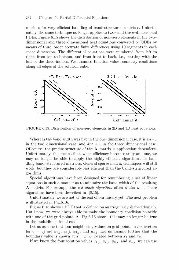
232 Chapter 6. Partial Differential Equations
routines for very efficient handling of band–structured matrices. Unfortu-nately, the same technique no longer applies to two– and three–dimensionalPDEs. Figure 6.15 shows the distribution of non–zero elements in the two–dimensional and three–dimensional heat equations converted to ODEs bymeans of third–order accurate finite differences using 10 segments in eachspace dimension. The differential equations were numbered from left toright, from top to bottom, and from front to back, i.e., starting with thelast of the three indices. We assumed function value boundary conditionsalong all edges of the solution cube.
2D Heat Equation 3D Heat Equation
Columns of AColumns of A
Row
sof
A
Row
sof
A
FIGURE 6.15. Distribution of non–zero elements in 2D and 3D heat equations.
Whereas the band width was five in the one–dimensional case, it is 4n+1in the two–dimensional case, and 4n2 + 1 in the three–dimensional case.Of course, the precise structure of the A–matrix is application dependent.Unfortunately, this means that, when efficiency becomes truly an issue, wemay no longer be able to apply the highly efficient algorithms for han-dling band–structured matrices. General sparse matrix techniques will stillwork, but they are considerably less efficient than the band–structured al-gorithms.
Special algorithms have been designed for renumbering a set of linearequations in such a manner as to minimize the band width of the resultingA–matrix. For example the red–black algorithm often works well. Thesealgorithms have been described in [6.15].
Unfortunately, we are not at the end of our misery yet. The next problemis illustrated in Fig.6.16.
Figure 6.16 shows a PDE that is defined on an irregularly shaped domain.Until now, we were always able to make the boundary condition coincidewith one of the grid points. As Fig.6.16 shows, this may no longer be truein the multidimensional case.
Let us assume that four neighboring values on grid points in x–directionfor y = yj are u1,j , u2,j , u3,j , and u4,j . Let us assume further that theboundary value is known at x = x1.35 located between x1 and x2.
If we know the four solution values u1,j , u2,j , u3,j , and u4,j , we can use
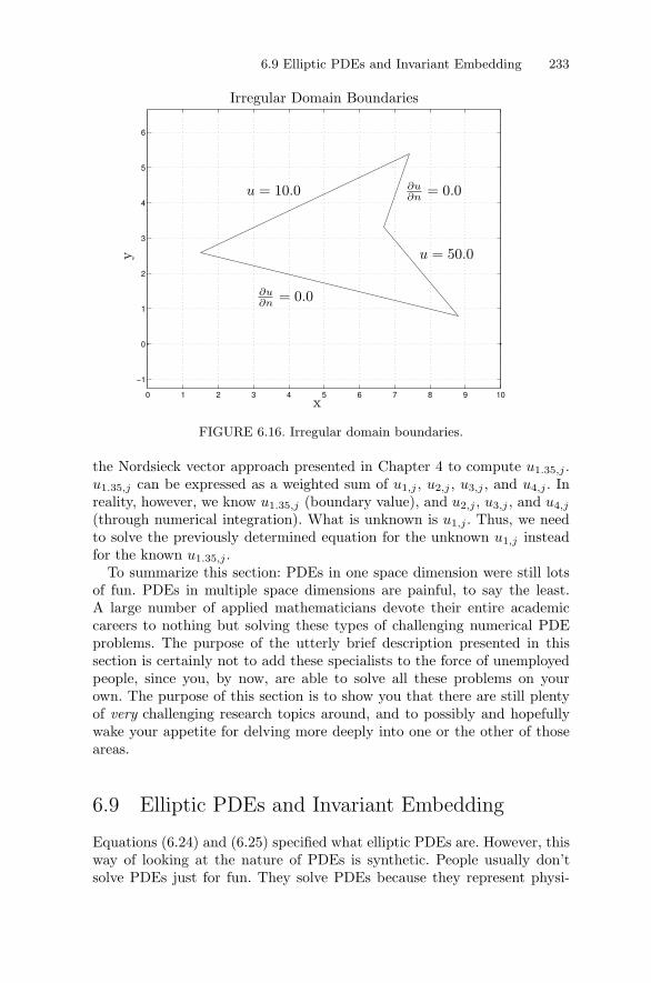
6.9 Elliptic PDEs and Invariant Embedding 233
0 1 2 3 4 5 6 7 8 9 10
−1
0
1
2
3
4
5
6
Irregular Domain Boundaries
x
y
u = 10.0
u = 50.0
∂u∂n = 0.0
∂u∂n = 0.0
FIGURE 6.16. Irregular domain boundaries.
the Nordsieck vector approach presented in Chapter 4 to compute u1.35,j .u1.35,j can be expressed as a weighted sum of u1,j , u2,j , u3,j , and u4,j . Inreality, however, we know u1.35,j (boundary value), and u2,j , u3,j , and u4,j
(through numerical integration). What is unknown is u1,j . Thus, we needto solve the previously determined equation for the unknown u1,j insteadfor the known u1.35,j .
To summarize this section: PDEs in one space dimension were still lotsof fun. PDEs in multiple space dimensions are painful, to say the least.A large number of applied mathematicians devote their entire academiccareers to nothing but solving these types of challenging numerical PDEproblems. The purpose of the utterly brief description presented in thissection is certainly not to add these specialists to the force of unemployedpeople, since you, by now, are able to solve all these problems on yourown. The purpose of this section is to show you that there are still plentyof very challenging research topics around, and to possibly and hopefullywake your appetite for delving more deeply into one or the other of thoseareas.
6.9 Elliptic PDEs and Invariant Embedding
Equations (6.24) and (6.25) specified what elliptic PDEs are. However, thisway of looking at the nature of PDEs is synthetic. People usually don’tsolve PDEs just for fun. They solve PDEs because they represent physi-

234 Chapter 6. Partial Differential Equations
cal problems that they are interested in. Physically meaningful parabolicPDEs represent predominantly heat diffusion or chemical reaction prob-lems, and physically meaningful hyperbolic PDEs describe field problemsin either hydrodynamics, electromagnetism, optics, general relativity the-ory, etc. Elliptic PDEs, on the other hand, are used to model stress andstrain problems in mechanical structural analysis.
The simplest elliptic PDE is the Laplace equation, e.g. in two spacedimensions:
∂2u
∂x2+
∂2u
∂y2= 0.0 (6.84)
Let us assume the Laplace equation is defined in a circular domain of radiusr = 1.0 around the origin. Since the domain is circular, it is much moreappropriate to formulate the problem using polar coordinates .
x = r · cos ϕ (6.85a)y = r · sin ϕ (6.85b)
or:
r =√
x2 + y2 (6.86a)
ϕ = arctan(y
x
)(6.86b)
We can express u(x, y) as u(r(x, y), ϕ(x, y)). Thus,
∂u
∂x=
∂u
∂r· ∂r
∂x+
∂u
∂ϕ· ∂ϕ
∂x(6.87)
or, in short–hand notation:
ux = ur · rx + uϕ · ϕx (6.88)
Using the chain rule and the multiplication rule, we find:
uxx + uyy =(r2x + r2
y
)urr + 2 (rxϕx + ryϕy) urϕ +
(ϕ2
x + ϕ2y
)uϕϕ
+ (rxx + ryy) ur + (ϕxx + ϕyy) uϕ (6.89)
or finally:
∂2u
∂r2+
1r· ∂u
∂r+
1r2
· ∂2u
∂ϕ2= 0.0 (6.90)
The boundary condition could be something like:

6.9 Elliptic PDEs and Invariant Embedding 235
∂u
∂r= f(ϕ, t) (6.91)
Notice that there is no need for any initial condition, since the PDE doesn’tdepend on time at all (except possibly through the boundary condition asin the above example). No numerical integration across time will take placeat all. We are thus in trouble with our MOL methodology.
In some cases, we might still be able to apply the MOL approach byeither differentiating along r and integrating along ϕ, or alternatively, bydifferentiating along ϕ and integrating along r. In both cases, however, wewould be lacking one initial condition, and would instead have one finalcondition too many. This is therefore not an initial value problem, butrather a boundary value problem. We haven’t discussed yet how those canbe solved.
Does this mean that we have to give up for the time being, or is there achance that we may turn this problem into one of our known initial valueproblems after all?
Let us simplify Eq.(6.91) a bit by assuming that the boundary conditiondoes not depend on time. In this case, the problem is totally static in nature,i.e., the solution is not time–dependent at all. The solution consists simplyof a set of u–values at the grid points.
We can now embed this problem within another problem as follows:
∂u
∂t=
∂2u
∂r2+
1r· ∂u
∂r+
1r2
· ∂2u
∂ϕ2(6.92)
with the boundary condition:
∂u
∂r= f(ϕ) (6.93)
and with arbitrary initial conditions.This is now clearly a parabolic initial value problem, which we already
know how to solve. Since the PDE is analytically stable, and since theboundary condition is not a function of time, the solution will eventuallysettle into a steady state. However, once the steady state has been reached,the solution no longer changes with time, thus:
∂u
∂t= 0.0 (6.94)
Therefore we conclude that the steady–state solution of the parabolic PDEis identical with the solution of the original elliptic PDE. This method ofsolving elliptic PDEs is called invariant embedding .1 Of course, the pricethat we have to pay for this comfort is formidable. We were able to convert
1A majority of the references spell “imbedding” with an “i” rather than with an “e,”probably because the inventor of the method didn’t have a dictionary handy when he

236 Chapter 6. Partial Differential Equations
a boundary value problem into an initial value problem at the expense ofincreasing the number of dimensions by one.
6.10 Finite Element Approximations
Those of you who read the companion book Continuous System Modeling[6.5] know our reservations against writing down mathematical formulaedeprived of their physical meaning. Mathematics is no end in itself. Math-ematics is simply the language of physics. Voltages and currents in an elec-tronic circuit don’t change their values as functions of time, because theyobserve some differential equations. They change their values in order tobring the system to a state of minimal energy. A differential equation isnot the cause that makes physics tick, it is only one way of describing,in mathematical terms and after the fact, what happens in the process ofenergy exchange taking place in the physical system.
You may remember also that there are two ways of looking at energyconservation laws:
1. We can look at the energy itself. In the most general case, we writedown a Hamiltonian or possibly a Hamiltonian field of the system(at least if the system is conservative), and from there, we can thenderive a set of differential equations if we so choose.
2. Rather than looking at the stored energy itself, we can look at incre-mental energies, i.e., at power flows . This leads directly to the bondgraph approach to modeling that was advocated in Chapters 7–9 ofthe companion book.
We strongly advocated the latter approach since power flow is a local prop-erty of the system, whereas energy is a global property of the system. Thus,power flow considerations lend themselves directly to an object–orientedapproach to modeling.
In distributed parameter system simulation, the situation is a little differ-ent. As explained earlier, the PDE models that we are dealing with todayare still structurally so simple that object orientation is of little concern.Also, especially if we are solving a boundary value problem anyway, as inthe case of the elliptic PDEs, we need to solve a global optimization prob-lem over the entire definition domain of the PDE, thus, the advantages ofa local model description are gone.
Looking at the solution of the previously discussed Laplace equation,we know that the solution will minimize the amount of energy stored in
wrote his first paper about the method . . . but we cannot bring ourselves to follow thetrend — it looks so ugly (!)
6.11 Summary 237
the system. Consequently, we can write an energy function parameterizedin the (unknown) solution values, and solve a minimization problem overthe set of unknown parameters. This leads to a set of algebraic equations,possibly nonlinear, in the unknown solution vector.
Approaches that follow this line of reasoning are called finite elementmethods. They come in many shades and colors. The technique was origi-nally developed by civil engineers trying to determine the static stress inbridges and other building structures. However, the method has a muchbroader range of possible applications. For all practical purposes, it can beviewed as an alternative to the finite difference approaches. Thus, it canconceptually also be used for other than elliptic PDEs.
The two approaches have their own particular advantages and disadvan-tages. Finite elements usually are less infected by problems with consistencyerrors than finite difference methods. Consequently, we can get by with alarger (and irregular) mesh, and thus, with a smaller number of equations.On the other hand, finite difference approximations always lead to sparsematrices. Finite element approximations do not share this property. As aconsequence, although the number of equations is smaller in the finite el-ement case, we may not be able to use sparse matrix techniques, and itis therefore not evident that the smaller system size truly leads to a moreeconomical algorithm. Also, a finite difference formulation is usually easierto derive and harder to solve than a finite element formulation. However, itis easier to incorporate irregular and even non–convex domain boundariesinto a finite element description.
Meanwhile, finite element methods have also been extended to the solu-tion of non–stationary problems by means of a Galerkin formulation [6.17].Thus, finite elements have suddenly become a contender to finite differenceseven in the context of the MOL methodology. However, more research inthis area is still needed.
6.11 Summary
In this chapter, we have first and primarily discussed the numerical solutionof PDEs in one space dimension. The method–of–lines approach lets usreduce such PDEs to large ODE systems that we can solve using regularODE software.
Parabolic PDEs lead to sets of (artificially) stiff ODEs that can be treatedappropriately using stiff system solvers such as the BDF algorithms. Sinceall of today’s continuous–system modeling and simulation environments,such as Dymola [6.7, 6.8], offer stiff system solvers as part of their simu-lation run–time library, it became clear that they are perfectly capable ofdealing with parabolic PDEs in one space dimension. The most cumber-some part in the conversion process was the derivation of the coefficients for

238 Chapter 6. Partial Differential Equations
the spatial finite difference approximations using Newton–Gregory polyno-mials, but this process can be easily automated.
Hyperbolic PDEs lead to large sets of marginally stable ODEs that canbest be solved by F–stable integration algorithms, such as the backinter-polation techniques. However, explicit algorithms, such as AB3 or RKF4/5may sometimes work just as well, as they avoid the need of computing ex-pensive Jacobians and inverse Hessians. Hyperbolic PDEs are numericallymore demanding than their parabolic cousins due to the occurrence of trav-eling shock waves. Adaptive moving mesh algorithms can provide a solutionto this problem, but then call for special–purpose software, since these al-gorithms are non–trivial in their implementation. It would be too muchof a burden to ask the user to implement such algorithms manually. Yet,powerful modeling environments can make also this process transparent tothe modeler.
Elliptic PDEs in one space dimension are no PDEs at all. They are oneclass of boundary value ODEs, and we shall discuss later in this book howthese can be tackled in general. However, one method was already providedhere, namely the method of invariant embedding, a method that convertsthe boundary value ODE into a parabolic PDE in one space dimension,with which we can then proceed as elaborated above.
Multidimensional PDEs were discussed next. Although they can, in prin-ciple, be treated in exactly the same manner as their one–dimensionalcounterparts, the numerical problems are formidable, and efficiency con-siderations become here an issue of utmost importance.
Does there exist general–purpose PDE software? We had already men-tioned the FORSIM–VI software [6.4]. FORSIM–VI is just a Fortran pro-gram. No preprocessor is involved at all. The user simply provides a Fortransubroutine describing his or her model. This makes FORSIM inappropriatefor use in more complex ODE situations, since not even an equation sorteris offered, lest an object–oriented modeling facility. What makes FORSIMdifferent from any other (simple–minded) ODE simulation system is thatFORSIM provides built–in subroutines for converting spatial derivativesinto finite difference approximations. These routines know how to computethe necessary coefficients, and consequently, the user doesn’t need to worryabout Newton–Gregory polynomials. FORSIM works with both equidis-tantly and non–equidistantly spaced grids. FORSIM also offers built–inroutines for converting general and even nonlinear boundary conditionsinto boundary value conditions. Thus, FORSIM helps the user tremen-dously with the encoding of his or her PDEs. Routines are available forconverting PDEs in one to three space dimensions, however, the two– andthree–dimensional routines are not general since they work only on rect-angular domains. FORSIM is strictly MOL–oriented. Spatial derivativesare discretized by means of finite difference approximations, whereas tem-poral derivatives are kept in the program for numerical integration acrosstime. FORSIM offers a Gear (BDF) algorithm for the solution of parabolic
6.11 Summary 239
problems, and an RKF4/5 algorithm for hyperbolic ones.A fairly similar software system is DSS/2 [6.16]. The two systems,
FORSIM–VI and DSS/2 are in fact so similar that a further discussionof DSS/2 can be skipped.
Other systems, such as PDEL [6.2], went another route. For the benefitof a more finely tuned numerical solution, they sacrificed generality forefficiency. These software systems allow the user to choose between a setof standard frequently occurring PDEs, and then employ different types of(not necessarily MOL) algorithms to solve the problem.
It may be noticed that all of these systems are fairly old. In the early sev-enties, it was hoped that PDE problems could be solved by general–purposePDE software just as ODE problems are solved by general–purpose ODEsoftware. This turned out to be an illusion. The ODE situation is muchsimpler. All we need to do is to provide a tool that allows to choose be-tween a set of different numerical integration algorithms, and we are inbusiness. Moreover, it often doesn’t matter too much what algorithm wechoose. One algorithm may be 30% faster or 20% slower than another, butwho cares. Modern PCs have become so powerful that they can effectivelyand efficiently deal with the simulation of a large majority of lumped pa-rameter models. In contrast, there exist many different techniques to solvePDE problems. Even if we limit our discussion to MOL–solutions, we mustchoose:
1. a numerical integration algorithm for integration across time,
2. a grid for discretization in space,
3. a numerical discretization scheme for differentiation across space,
4. an algorithm to translate boundary conditions specified at an arbi-trary point in space to boundary conditions specified at the nearestgrid point
5. an algorithm for converting general boundary conditions to boundaryvalue conditions,
and this is only one among many approaches for numerically solving PDEs.Furthermore, the sensitivity of the solution to the selection of just the rightcombination of algorithms is much greater in the PDE case than in the ODEcase. Selecting one method may mean that we have to wait for 50 hoursuntil we obtain a (hopefully correct) answer, whereas the same problemmay be solved by the best possible combination of algorithms in just a fewseconds.
For these reasons, general–purpose PDE software hasn’t lived up to itspromise. The “casual” user of PDE software cannot be protected from hav-ing to understand the intricacies of the underlying numerical algorithms,and the numerical solution to all but toy PDE problems is so expensive

240 Chapter 6. Partial Differential Equations
that it is well worth spending some time on understanding what is goingon before starting to crunch numbers. Getting coefficients out of Newton–Gregory polynomials may be but the least of our problems.
The situation is somewhat different in the case of elliptic PDEs. EllipticPDEs are the simplest and most benign of all PDE problems. An extensiveeffort was undertaken by John Rice and his colleagues with large amountsof funding through the national agencies to solve that problem once and forall. They designed the ELLPACK software [6.15]. ELLPACK started outas a collection of useful algorithms to solve general–purpose elliptic PDEsin two and three space dimensions.
It turned out that the situation became soon too messy. Casual usersno longer could learn to use these algorithms without help from the pro-fessional. To remedy the situation, a simple language was designed, and acompiler was written that would translate programs written in that lan-guage into a Fortran program that would then invoke the previously dis-cussed algorithms that now form part of the run–time library. Thus, bythis time, we are in the same situation as with the continuous–system sim-ulation languages.
It turned out that it didn’t work. The approach was too simple–minded.As a new algorithm became available, new keywords had to be added tothe language in order to make this new algorithm accessible, and conse-quently, the compiler had to be updated frequently. This became too muchof a hassle to the software designers. So they decided to parameterize thecompiler. The compiler was generated out of a data template file that de-scribed both syntax and semantics of the ELLPACK language by meansof a compiler–compiler . So, from now on, new features needed only to beincorporated into the data template file, and a new compiler for the somodified language could be generated at once.
Well, you may already have guessed . . . it didn’t work. The researchersfound the manual generation of the data template file much too cumber-some after all. That problem was taken care of easily. The precise detailsof the data template file were generated by a data template compiler outof a more abstract description of the data template file. Of course, alsothe data template compiler wasn’t hand–coded. Why should it? Instead,the data template compiler was generated out of an abstract descriptionof its duties by the same compiler–compiler that also generates the ELL-PACK language compiler. This allows us to also update the data templatecompiler easily and readily.
At this point in time, only one question remains: Who wrote the compiler–compiler? We assume most of you read the story of Munchhausen whopulls himself out of the swamp by pulling on his own hair . . . the compiler–compiler wrote itself. A first (bootstrap) version of the compiler–compilerwas hand–coded. This version was already able to read a language descrip-tion in terms of its syntax and semantics. Well, the first language descrip-tion it got to read was its own. So, by running the bootstrap compiler–

6.12 References 241
compiler through a description of itself, a second and much cleaner versionof the compiler–compiler was obtained that could subsequently be usedto generate new versions of the ELLPACK language compiler, the datatemplate compiler, and –why not– itself.
Was it worth it? As an intellectual stimulus, most certainly. As an ex-perimental toolbox for solving new kinds of elliptic PDEs, probably. As ageneral–purpose production tool for solving specific PDE problems posedin industry, not likely. We acquired the tool some years ago when we helda contract from the microelectronic industry to design a device simulatorthat could predict the breakdown behavior of bipolar power transistors (ef-fectively, of any kind of reverse–biased p–n junction). The results that weobtained using ELLPACK were documented in [6.18]. ELLPACK allowedus to fairly quickly and easily go through a number of different algorithmsand gain a feeling for which combination of algorithms might work decentlywell. However, the simulations obtained in this manner were painfully slow.A simple p–n junction milled for an hour or two on a VAX 11/780. Morecomplex devices could not be handled at all within reasonable time lim-its. Therefore, we then designed our own special–purpose device simulator,ASEPS [6.19]. This program was able to simulate simple p–n junctionsin a few seconds of CPU time on the same machine. ASEPS then enabledus to also study more complex device structures such as special geomet-ric configurations of device termination structures for radiation–hardenedpower MOSFETs [6.6]. These simulation runs took a few minutes each,and optimization studies could be performed in batch mode over night.
Good special–purpose finite element software for structural analysis, suchas NASTRAN, has been around for some time. This software doesn’t at-tempt to solve general–purpose elliptic PDEs. Only one type of problemis solved, but the program is very flexible with respect to the specificationof the domain on which the problem is to be solved and with respect tothe selection of grid points (finite element programs aren’t limited to usingrectangular grids). Special–purpose numerical PDE solvers exist also forseveral other classes of applications, such as fluid dynamics.
It is disappointing to a generalist that the general–purpose approach tonumerical PDE solution didn’t work out. Unfortunately, we don’t see anycure yet. Consequently, special–purpose solutions for specific PDE problemswill be around for years to come.
6.12 References
[6.1] Kathryn E. Brenan, Stephen L. Campbell, and Linda R. Petzold.Numerical Solution of Initial–Value Problems in Differential–AlgebraicEquations. North–Holland, New York, 1989. 256p.
[6.2] Alfonso F. Cardenas and Walter J. Karplus. PDEL — A Language
242 Chapter 6. Partial Differential Equations
for Partial Differential Equations. Comm. ACM, 13:184–191, 1970.
[6.3] Michael B. Carver and H.W. Hinds. The Method of Lines and theAdvective Equation. Simulation, 31:59–69, 1978.
[6.4] Michael B. Carver, D.G. Stewart, J.M. Blair, and W.M. Selander.The FORSIM VI Simulation Package for the Automated Solutionof Arbitrarily Defined Partial and/or Ordinary Differential EquationSystems. Technical Report AECL–5821, Chalk River Nuclear Lab-oratories, Atomic Energy of Canada Limited, Chalk River, Ontario,Canada., 1978.
[6.5] Francois E. Cellier. Continuous System Modeling. Springer Verlag,New York, 1991. 755p.
[6.6] Kenneth R. Davis, Ronald D. Schrimpf, Kenneth F. Galloway,and Francois E. Cellier. The Effects of Ionizing Radiation onPower–MOSFET Termination Structures. IEEE Trans. Nuclear Sci.,36(6):2104–2109, 1989.
[6.7] Hilding Elmqvist. A Structured Model Language for Large ContinuousSystems. PhD thesis, Dept. of Automatic Control, Lund Institute ofTechnology, Lund, Sweden, 1978.
[6.8] Hilding Elmqvist. Dymola — Dynamic Modeling Language, User’sManual, Version 5.3. DynaSim AB, Research Park Ideon, Lund, Swe-den, 2004.
[6.9] C. William Gear. Numerical Initial Value Problems in Ordinary Dif-ferential Equations. Series in Automatic Computation. Prentice–Hall,Englewood Cliffs, N.J., 1971. 253p.
[6.10] J. Mack Hyman. Moving Mesh Methods for Partial DifferentialEquations. In Jerome A. Goldstein, Steven Rosencrans, and Gary A.Sod, editors, Mathematics Applied to Science: In Memoriam EdwardD. Conway, pages 129–153. Academic Press, Boston, Mass., 1988.
[6.11] John D. Lambert. Numerical Methods for Ordinary Differential Sys-tems: The Initial Value Problem. John Wiley, New York, 1991. 304p.
[6.12] R. Ivan Lewis. Vortex Element Methods for Fluid Dynamic Analysisof Engineering Systems. Cambridge University Press, New York, 1991.588p.
[6.13] Anthony Ralston and Herbert S. Wilf. Mathematical Methods forDigital Computers. John Wiley & Sons, New York, 1960. 287p.
[6.14] John R. Rice and Ronald F. Boisvert. Solving Elliptic ProblemsUsing Ellpack. Springer–Verlag, New York, 1985. 497p.

6.13 Bibliography 243
[6.15] Robert D. Richtmyer and K. William Morton. Difference Methodsfor Initial Value Problems. Wiley Interscience, New York, 1967. 405p.
[6.16] William E. Schiesser. The Numerical Method of Lines: Integrationof Partial Differential Equations. Academic Press, San Diego, Calif.,1991. 326p.
[6.17] V. Rao Vemuri and Walter J. Karplus. Digital Computer Treatmentof Partial Differential Equations. Prentice–Hall, Englewood Cliffs,N.J., 1981. 449p.
[6.18] Qiming Wu and Francois E. Cellier. Simulation of High–VoltageBipolar Devices in the Neighborhood of Breakdown. Mathematics andComputers in Simulation, 28:271–284, 1986.
[6.19] Qiming Wu, Chimin Yen, and Francois E. Cellier. Analysis of Break-down Phenomena in High–Voltage Bipolar Devices. Transactions ofSCS, 6(1):43–60, 1989.
6.13 Bibliography
[B6.1] Myron B. Allen, Ismael Herrera, and George F. Pinder. NumericalModeling in Science and Engineering. John Wiley & Sons, New York,1988. 418p.
[B6.2] William F. Ames. Numerical Methods for Partial Differential Equa-tions. Academic Press, New York, 3rd edition, 1992. 433p.
[B6.3] T. J. Chung. Computational Fluid Dynamics. Cambridge Univer-sity Press, Cambridge, United Kingdom, 2002. 800p.
[B6.4] Peter S. Huyakorn and George F. Pinder. Computational Methodsin Subsurface Flow. Academic Press, New York, 1983. 473p.
[B6.5] Leon Lapidus and George F. Pinder. Numerical Solution of Par-tial Differential Equations in Science and Engineering. John Wiley &Sons, New York, 1999. 677p.
[B6.6] Robert Vichnevetsky and John B. Bowles. Fourier Analysis of Nu-merical Approximations of Hyperbolic Equations. SIAM Publishing,Philadelphia, Penn., 1982. 140p.
[B6.7] John Keith Wright. Shock Tubes. John Wiley & Sons, New York,1961. 164p.
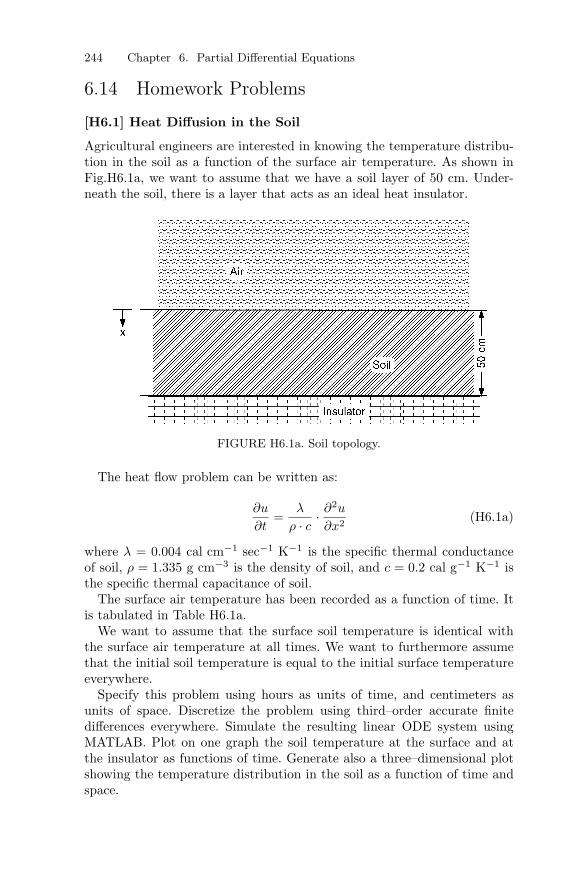
244 Chapter 6. Partial Differential Equations
6.14 Homework Problems
[H6.1] Heat Diffusion in the Soil
Agricultural engineers are interested in knowing the temperature distribu-tion in the soil as a function of the surface air temperature. As shown inFig.H6.1a, we want to assume that we have a soil layer of 50 cm. Under-neath the soil, there is a layer that acts as an ideal heat insulator.
x
FIGURE H6.1a. Soil topology.
The heat flow problem can be written as:
∂u
∂t=
λ
ρ · c · ∂2u
∂x2(H6.1a)
where λ = 0.004 cal cm−1 sec−1 K−1 is the specific thermal conductanceof soil, ρ = 1.335 g cm−3 is the density of soil, and c = 0.2 cal g−1 K−1 isthe specific thermal capacitance of soil.
The surface air temperature has been recorded as a function of time. Itis tabulated in Table H6.1a.
We want to assume that the surface soil temperature is identical withthe surface air temperature at all times. We want to furthermore assumethat the initial soil temperature is equal to the initial surface temperatureeverywhere.
Specify this problem using hours as units of time, and centimeters asunits of space. Discretize the problem using third–order accurate finitedifferences everywhere. Simulate the resulting linear ODE system usingMATLAB. Plot on one graph the soil temperature at the surface and atthe insulator as functions of time. Generate also a three–dimensional plotshowing the temperature distribution in the soil as a function of time andspace.

6.14 Homework Problems 245
t [hours] u oC0 66 16
12 2818 2124 1836 3448 1860 2566 1572 4
TABLE H6.1a. Surface air temperature.
[H6.2] Electrically Heated Rod
We start out with a simple parabolic partial differential equation describingthe temperature distribution in an electrically heated copper rod. Thisphenomenon can be modeled by the following equation:
∂T
∂t= σ
(∂2T
∂r2+
1r· ∂T
∂r+
Pelectr
λ · V)
(H6.2a)
The first two terms represent the standard diffusion equation in polar co-ordinates as described previously in Eq.(6.92), and the constant term de-scribes the electrically generated heat. It can be derived from Fig.8.13 ofthe companion book on Continuous System Modeling [6.5].
σ =λ
ρ · c (H6.2b)
is the diffusion coefficient, where λ = 401.0 J m−1 sec−1 K−1 is the specificthermal conductance of copper, ρ = 8960.0 kg m−3 is its density, andc = 386.0 J kg−1 K−1 is the specific thermal capacitance.
Pelectr = u · i (H6.2c)
is the dissipated electrical power, and
V = π · R2 · � (H6.2d)
is the volume of the rod with the length � = 1 m and the radius R =0.01 m. The rod is originally in an equilibrium state at room temperatureTroom = 298.0 K.

246 Chapter 6. Partial Differential Equations
The boundary conditions are:
∂T
∂r
∣∣∣∣r=0.0
= 0.0 (H6.2e)
∂T
∂r
∣∣∣∣r=R
= −k1
(T (R)4 − T 4
room
)− k2 (T (R) − Troom) (H6.2f)
where the quartic term models the heat radiation, whereas the linear termmodels convective heat flow away from the rod.
We want to simulate this system using the MOL approach with 20 spa-tial segments (in radial direction), and using second–order accurate finitedifference approximations for the first–order spatial derivatives, and third–order accurate finite differences for the second–order spatial derivatives.We are going to treat the boundary condition at the center as a generalboundary condition rather than as a symmetry boundary condition in orderto circumvent the difficulties with computing the term (∂T/∂r)/r, whichevaluates to 0/0 at r = 0.0.
For internal segments, we obtain thus differential equations of the type:
dTi
dt≈ σ
(Ti+1 − 2Ti + Ti−1
δr2+
1r· Ti+1 − Ti−1
2δr+
Pelectr
λ · V)
(H6.2g)
which are straightforward to implement. For the left–most segment, wehave the condition:
∂T
∂r
∣∣∣∣r=0.0
= 0.0 ≈ 12δr
(−T3 + 4T2 − 3T1) (H6.2h)
and therefore:
T1 ≈ 43T2 − 1
3T3 (H6.2i)
Consequently, we don’t need to solve a differential equation at r = 0.0, andthereby, we skip the 0/0 division.
At the right–most segment, we obtain:
∂T
∂r
∣∣∣∣r=R
= −k1
(T 4
21 − T 4room
)−k2 (T21 − Troom) ≈ 12δr
(−3T21 + 4T20 − T19)
(H6.2j)Thus, we obtain a nonlinear equation in the unknown T21:
F(T21) = k1
(T 4
21 − T 4room
)+ k2 (T21 − Troom) − 1
2δr(−3T21 + 4T20 − T19)
≈ 0.0 (H6.2k)

6.14 Homework Problems 247
which can be solved by Newton iteration:
T 021(t) = T21(t − h) (H6.2l)
T 121(t) = T 0
21(t) −F(T 0
21)H(T 0
21)(H6.2m)
T 221(t) = T 1
21(t) −F(T 1
21)H(T 1
21)(H6.2n)
until convergence
where:H(T21) =
∂F∂T21
= 4k1T321 + k2 − 3
2δr(H6.2o)
[H6.3] Wave Equation
The wave equation has been written as:
∂2u
∂t2= c2 · ∂2u
∂x2(H6.3a)
Let us rewrite u(x, t) as u(v, w), where:
v = t + x (H6.3b)w = t − x (H6.3c)
What happens?
[H6.4] Shock Tube Simulation
We wish to analyze the influence of α and β on the accuracy of the sim-ulation. Repeat the same 50 segment simulation with different values forα and β. What do you conclude about the relative influence of α and βin comparison with the consistency error. Assuming a small value of α,which is the largest value of β acceptable before the relative error exceeds1%. Similarly, assuming a small value of β, which is the largest value of αacceptable before the relative error exceeds 1%.
Use one half the maximum values of α and β found above, and simulateacross a longer period of time. Can you reach steady–state? Interpret theresults.
[H6.5] River Bed Simulation
Hydrologists are interested in determining the movement of river beds withtime. The dynamics of this system can be described through the PDE:
∂v
∂t+ v · ∂v
∂x+ g · ∂h
∂x+ g · ∂z
∂x= w(v) (H6.5a)

248 Chapter 6. Partial Differential Equations
where v(x, t) is the absolute value of the flow velocity of the water, h(x, t)is the water depth, and z(x, t) is the altitude of the river bed relative to anarbitrary constant level. g = 9.81 m sec−2 is the gravitational constant.
w(v) is the friction of water at the river bed:
w(v) = − g · v2
s2k · h4/3
(H6.5b)
where sk = 32.0 m3/4 sec−1 is the Strickler constant.The continuity equation for the water can be written as:
∂h
∂t+ v · ∂h
∂x+ h · ∂v
∂x= 0.0 (H6.5c)
and the continuity equation for the river bed can be expressed as:
∂z
∂t+
df(v)dv
· ∂v
∂x= 0.0 (H6.5d)
where f(v) is the transport equation of Meyer–Peter simplified by meansof regression analysis:
f(v) = f0 + c1(v − v0)c2 (H6.5e)
where c1 = 1.272 · 10−4 m, and c2 = 3.5.We want to study the Rhine river above Basel over a distance of 6.3 km.
We want to simulate this system across 20 days of simulated time. Theinitial conditions are tabulated in Table H6.5a.
x [m] v [m/s] h [m] z [m]0.0 2.3630 3.039 59.82
630.0 2.3360 3.073 59.061260.0 2.2570 3.181 58.291890.0 1.6480 4.357 56.752520.0 1.1330 6.337 54.743150.0 1.1190 6.416 54.603780.0 1.1030 6.509 54.454410.0 1.0620 7.001 53.915040.0 0.8412 8.536 52.365670.0 0.7515 9.554 51.336300.0 0.8131 8.830 52.02
TABLE H6.5a. Initial data for river bed simulation.
We need three boundary conditions. We want to assume that the amountof water q = h · v entering the simulated river stretch is constant. Forsimplicity, we shall assume both h and v constant. At the lower end, thereis a weir. Therefore, we can assume that the sum of z and h is constant

6.14 Homework Problems 249
at the lower end of the simulated stretch of river. Since the water movesmuch faster than the river bed, it doesn’t make too much sense to applyboundary conditions to the river bed.
This system is pretty awful. The time constants of the water are measuredin seconds, whereas those of the ground are measured in days. We areinterested in the slow time constant, yet it is the fast time constant thatdictates the integration step size. We can think of the first two PDEs asa nonlinear function generator for the third PDE. Let us therefore modifyEq.(H6.5d) as follows:
∂z
∂t+ β · df(v)
dv· ∂v
∂x= 0.0 (H6.5f)
The larger we choose the tuning parameter, the faster will the river bedmove. Select a value somewhere around β = 100 or even β = 1000. Later,we must analyze the damage that we did to the PDE system by introducingthis tuning parameter. Maybe, we can extrapolate to the correct systembehavior at β = 1.0.
The third boundary condition is analytically correct, but numericallynot very effective since it is specified at the wrong end of the system. Sincewater always flows downhill, a boundary condition at the bottom is aboutas effective as commanding my dog to solve this homework problem. Letus therefore introduce yet another boundary condition at the top end:
∂z
∂x= constant (H6.5g)
However, since we cannot specify a derivative boundary condition for afirst–order equation, we reformulate Eq.(H6.5g) as:
z1 = z2 + constant (H6.5h)
Plot the river bed altitude z(x) measured at the end of every five day periodsuperposed onto one graph.
Rerun the simulation for different values of β. Is it possible to extrapolatewhat the solution would look like for β = 1.0?
[H6.6] Boundary Value Conversion
A PDE in one space dimension is specified in the range [0.0,1.0] with δx =0.1. Unfortunately, one of the boundary values if given as: u(x = 0.98, t) =f(t).
We want to translate this boundary value to an equivalent boundaryvalue at u(x = 1.0, t). Use the Nordsieck vector approach to come upwith a third–order accurate equation for u(x = 1.0, t) as a function ofu(x = 0.98, t), u(x = 0.9, t), u(x = 0.8, t), and u(x = 0.7, t).
[H6.7] Coordinate Transformation
Verify that Eq.(6.92) is indeed correct.

250 Chapter 6. Partial Differential Equations
[H6.8] Coordinate Transformation
We wish to solve the Laplace equation for diffusion along the surface of aglobe, assuming that no diffusion takes place in radial direction. To thisend, we start out with the three–dimensional Laplace equation:(
∂2
∂x2+
∂2
∂y2+
∂2
∂z2
)u(x, y, z) = 0.0 (H6.8a)
We want to rewrite this Laplace equation as a function of three differentcoordinates:
u(x, y, z) = u(ρ, ξ, η) (H6.8b)
where ρ is the radius of the globe, ξ is the longitude, and η is the latitude.We obtain a modified Laplace equation in these coordinates. We then spec-ify that:
∂2u
∂ρ2=
∂u
∂ρ= 0.0 (H6.8c)
It is easy to make mistakes in such transformations. We therefore want tocheck whether the result is at least potentially correct. To this end, we letρ → ∞. Obviously, this must give us the original Laplace equation back,now expressed in ξ and η instead of x and y.
[H6.9] Poiseuille Flow Through a Pipe
The following equations describe the stationary flow of an incompressiblefluid through a pipe:
dv
dρ=
−√2Γ
(τM + 1)2· ρ · τ2 (H6.9a)
d
dρ
(ρ
T· dτ
dρ
)=
−Γ(τM + 1)3
· ρ3 · τ2 (H6.9b)
where:
ρ =r
R(H6.9c)
τ =T (r)TW
(H6.9d)
are two normalized coordinates. r is the distance from the center of thepipe, and R is the radius of the pipe. T (r) is the temperature of the fluidat a distance r from the center, and TW is the temperature of the pipe wall.TW is assumed constant. v = k1 ∗ v is the normalized flow velocity, where
6.15 Projects 251
k1 is a constant that depends on the viscosity, the thermal conductivity,and the average temperature of the fluid.
The boundary conditions are:
dv
dρ(ρ = 0.0) = 0.0 (H6.9e)
dτ
dρ(ρ = 0.0) = 0.0 (H6.9f)
v(ρ = 1.0) = 0.0 (H6.9g)τ(ρ = 1.0) = 1.0 (H6.9h)
Thus, this is a boundary value problem. We could integrate this problemacross ρ in the range ρ = [0.0, 1.0] with unknown initial conditions v(ρ =0.0) = vM and τ(ρ = 0.0) = τM .
However, in the light of what we learnt in this chapter, we shall tryanother approach. We embed this boundary value problem into a parabolicPDE, which we solve with arbitrary initial conditions until we reach steady–state.
Notice that the equations contain two yet unknown parameters. Γ is aconstant that depends on the fluid. Let us assume that Γ = 10.0. τM is thevalue of the normalized temperature at the center of the pipe. We simplyintroduce the momentary value of that temperature into the equation, andmodify that value as the simulation proceeds.
6.15 Projects
[P6.1] Grid–Width Control
Implement a moving grid algorithm for the shock tube problem using theideas that were outlined in this chapter.
6.16 Research
[R6.1] Grid–Width Control
Generalize the idea of a moving grid algorithm to hyperbolic PDEs in twospace dimensions.
Develop a general theory for assessment of the consistency error, andderive a grid–width control algorithm that contains the consistency errorin a reliable and systematic fashion.