Partial Differential Equations

Finite Difference Approximation

A Partial Differential Equation is simply defined as an equation involving partial derivatives of two or more independent variables.

For example, for the function in two independent variables f(x,y), the two partial derivatives are defined as:

y)y,x(f)yy,x(f

limyf

andx

)y,x(f)y,xx(flim

xf

0y0x

A general expression for a Linear Second-Order PDE in two variables would be:

0Dyf

Cyxf

Bxf

A 2

22

2

2

This type of equation is very useful in a number of engineering applications

The most useful types of PDEs are the following (again, in two spatial dimensions or one dimension + time )

Elliptic

Parabolic

Hyperbolic

0yT

xT

2

2

2

2

TxT

k 2

2

2

2

22

2 fc1

xf

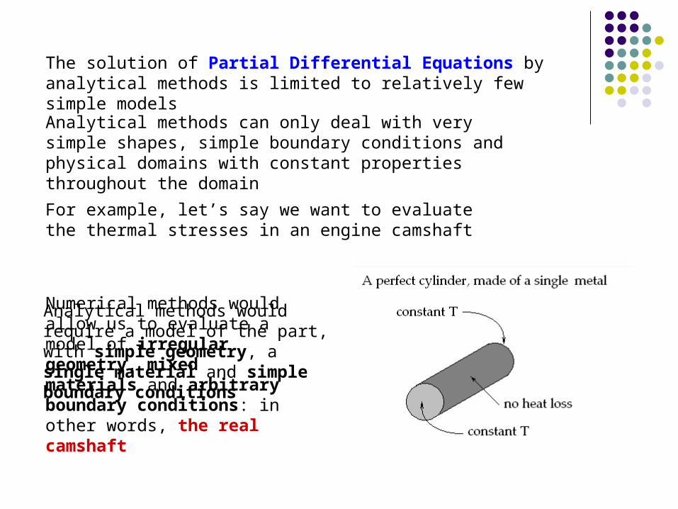
The solution of Partial Differential Equations by analytical methods is limited to relatively few simple models

Analytical methods can only deal with very simple shapes, simple boundary conditions and physical domains with constant properties throughout the domain

For example, let’s say we want to evaluate the thermal stresses in an engine camshaft

Numerical methods would allow us to evaluate a model of irregular geometry, mixed materials and arbitrary boundary conditions: in other words, the real camshaft

Analytical methods would require a model of the part, with simple geometry, a single material and simple boundary conditions

Elliptic PDEs

The Laplace Equation

Let’s review a simple case

Consider the case of a 12 ft. x 12 ft. thin steel plate, perfectly insulated on both sides and touching a pipe that carries steam at 150o C:

The temperature at this edge should be 150o C

Let’s say that the temperature at the other three edges is 20o C

What would be the temperature distribution at all internal points within the plate?

The expression that models this 2-D steady-state problem is Laplace’s Equation:

0yT

xT

2

2

2

2

Each of the terms can be represented by a Centered Second-Order Approximation, as we did for ODEs:

2

1j,iij1j,i

2

j,1iijj,1i

h

TT2Tand

h

TT2T

Note that the sum of these terms is equal to zero, which allows us to eliminate the h2 terms (assuming we use the same h in the x and y directions !)

In two spatial dimensions, we can avoid the double subindices by the use of a visual grid:

In the X direction In the Y direction

1 1

1

1

-2- 2

…but when we combine the two, we generate some overlaps

- 4

To generate the equation set, we superimpose this 5-point template on each interior node

Now we need a discretization grid for our problem

Using an h = 3 ft we would create the following grid:

There are 9 internal nodes in this grid

To generate the equations, we follow the same procedure as with the Boundary Value ODEs

First we express the equation for each interior node…

…and then we incorporate the boundary conditions

The following single-index node numbering will facilitate the process of writing the equations:

T = 20 at these nodes

… and also at these

…and here

Finally, T = 150 at these nodes

Now we write the equations

To illustrate how to use the “4-point star” scheme to write the applicable equations, let’s do node 7

This is what the “star” looks like for node 7:

This leads to the following equation:

T4 – 4 T7 + T8 + 20 + 150 = 0 or

T4 – 4 T7 + T8 = - 170

Note that the nodes are ordered according to their indices

Using the same procedure, we can develop the complete 9 x 9 system of equations

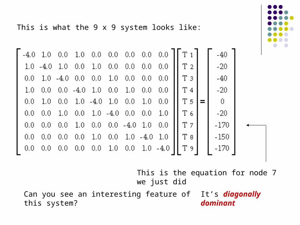
This is what the 9 x 9 system looks like:

This is the equation for node 7 we just did

Can you see an interesting feature of this system? It’s diagonally dominant

Solving the system in Excel produces the following results:

T1 = 29.2857

T2 = 32.7679

T3 = 29.2857

T4 = 44.3750

T5 = 52.5000

T6 = 44.3750

T7 = 75.7143

T8 = 88.4821

T9 = 75.7143

…and this is a crude diagram of selected isotherms

30oC

50oC

80oC

Perhaps you notice the symmetry in the diagram…

…which is a very useful characteristic of this system

Why is symmetry useful in this case?

Because it will allow us to use a finer discretization with a modest increase of the size of the system to be solved

We can use h = 2, which will force more nodes in the “y” direction…

…but will use a total of just 15 internal nodes (in other words, a 15 x 15 system – less than twice those of the first attempt)

However, the effective number of internal nodes will increase to 25 (because of the symmetry)

Let’s have a look at the node diagram

This is what our finer grid looks like:

It has a total of 15 internal nodes

Boundary conditions on these sides are still T = 20o C

…and T=150o C on this side

…but what are the boundary conditions on this side?

In general, Boundary Conditions for an Elliptic Partial Differential Equation of the form:

0zf

yf

xf

ofversioncondensedtheiswhich0f

2

2

2

2

2

2

2

…can be of the following two types:

Dirichlet conditions (value known)

Neumann conditions (gradient known)

k)z,y,x(f iii

kxf

iii z,y,x

In our case, the left boundary of our domain (a line defined by x = constant) is also an axis of symmetry

This means that the boundary is like a mirror: points of the function would have the same value as their reflection

The points shown are mirror images of each other (same y, equal x of opposite sign), and hence have the same functional value

(this is true for any value of h !)

This means that any centered approximation we care to use for the first derivative will result in a value of zero for this derivative at the edge

Another case where this must be true is at an isolated boundary: since no heat flux is permitted, the temperature gradient must be zero

In practical terms, this means that we have to adjust our “star shaped” template for the partial derivatives:

This temperature

…is equal to this temperature

We can “fold the edge” to reflect this

The 15 x 15 system of equations looks like this

The numerical results are:

Axis of simmetry

107.025 101.799 80.929

T = 150o C on this boundary

T = 20o C

on th

is bou

ndary

37.997 35.758 29.332

52.500 48.750 37.500

74.503 69.242 51.918

T = 20o C on this boundary

27.975 26.951 24.071

The isotherm diagram resulting from the refined mesh is

30o C

40o C

60o C

100o C

Note that symmetry allowed us to deal only with the shaded half

Without the use of symmetry, we would have needed 25 internal nodes, and hence a 25 x 25 system of equations, instead of the 15 x 15 we just solved

Earlier in this class I praised Numerical Methods for PDEs, for their ability to deal with real problems, not idealized models of reality

There are three main issues that limit analytical methods:

1. Irregular geometry

2. Arbitrary boundary conditions, and

3. Non-homogeneous material properties

Methods based on Finite Difference Approximations (such as the examples we have seen today), can only deal with the first two issues

To deal with anisotropy (non-constant properties in the medium, perhaps due to the use of mixed materials of construction), we would need to use the Finite Element Method

Arbitrary boundary conditions we have already used; let’s discuss how arbitrary geometry can be dealt with, using the Finite Difference Method

Say you want to model the face of Homer SimpsonWell, just the 2-D profile .You would have to decide on a mesh size, and place it over the model

…and then trim the mesh to approximate the model

You will have to find a mesh size that is practical, and yet accurate enough

Let’s try another problem in Excel

The boiler support problem

(A problem with a high degree of bogusity)

Imagine a tank, in use for storage of boiling water

The tank is made of metal plates, supported from the inside with semi-circular concrete columns

The circular surface of the column is in contact with boiling water (100oC)

The flat surface of the column is in contact with the metal wall (essentially at 0oC)

A cross section of the column

Since the temperatures are the same along the "vertical" dimension z, this can be modeled as a 2-D problem

We want the temperature at this point, which is located at the horizontal center, a distance equal to 0.6R from the "cold side"

Overlaying the grid

The first step to discretization is to lay a square grid over the domain

The actual contour is hard to replicate

This is the best we can do*

We'll assume we know T at the "white" nodes

...and make use of symmetry along this side

* given the limitations of the grid size we have chosen!

The final grid

Even a coarse grid, with symmetry, results in a fairly large number of nodes

We want the T at this node (analytical solution is T = 68.8083 oC)

Let's have a look at the Excel solution, compared to the analytical solution

And now, an assignment

A flat plate made of an experimental metal alloy is insulated on both sides, and subjected to the following boundary conditions: Along the top side: 400o F Along the right side: 160o F

Along the bottom side: 35o F Along the left side: 80oF

The purpose of the experiment is to measure the heat conductivity of the metal under transient conditions, keeping the boundary temperatures constant. At the end of the experiment, the plate is allowed to reach steady state; in steady state conditions, the temperature distribution can be modeled by the Laplace Equation:

0yT

xT

2

2

2

2

The plate measures 60 inches in width and 40 inches in height; hence, the grid spacing is uniform in both “x” and “y” directions, and it is Δx = Δy = 10 inches. Your task is to calculate the required nodal temperatures at steady state, using the grid shown in the diagram provided below. Specifically, you must predict the temperature to be measured at nodes P, Q and Z.

(From a recent final exam!)