finite element analyses of differential shrinkage …
TRANSCRIPT

FINITE ELEMENT ANALYSES OF DIFFERENTIAL SHRINKAGE-INDUCED
CRACKING IN CENTRIFUGALLY CAST CONCRETE POLES
A THESIS SUBMITTED TO THE GRADUATE SCHOOL OF NATURAL AND APPLIED SCIENCES
OF MIDDLE EAST TECHNICAL UNIVERSITY
BY
TUĞRUL TANFENER
IN PARTIAL FULFILLMENT OF THE REQUIREMENTS FOR
THE DEGREE OF MASTER OF SCIENCE IN
CIVIL ENGINEERING
SEPTEMBER 2012

Approval of the thesis:
FINITE ELEMENT ANALYSES OF DIFFERENTIAL
SHRINKAGE-INDUCED CRACKING IN CENTRIFUGALLY CAST CONCRETE POLES
submitted by TUĞRUL TANFENER in partial fulfillment of the requirements for the degree
of Master of Science in Civil Engineering Department, Middle East Technical University by,
Prof. Dr. Canan Özgen
Dean, Graduate School of Natural and Applied Sciences ___________
Prof. Dr. Güney Özcebe Head of Department, Civil Engineering ___________
Asst. Prof. Dr.Serdar Göktepe Supervisor, Civil Engineering Dept., METU ___________
Prof. Dr. İsmail Özgür Yaman
Co-supervisor, Civil Engineering Dept., METU ___________
Examining Committee Members:
Prof. Dr. Barış Binici
Civil Engineering Dept., METU ___________
Asst. Prof. Dr. Serdar Göktepe
Civil Engineering Dept., METU ___________
Prof. Dr. İsmail Özgür Yaman
Civil Engineering Dept., METU ___________
Assoc. Prof. Dr. Afşin Sarıtaş Civil Engineering Dept., METU ___________
Asst. Prof. Dr. Ercan Gürses Aerospace Engineering Dept., METU ___________
Date: 06.09.2012

iii
I hereby declare that all information in this document has been obtained and
presented in accordance with academic rules and ethical conduct. I also declare
that, as required by these rules and conduct, I have fully cited and referenced all
material and results that are not original to this work.
Name, Last Name: TUĞRUL TANFENER
Signature:
iv
ABSTRACT
FINITE ELEMENT ANALYSES OF DIFFERENTIAL SHRINKAGE-INDUCED CRACKING IN CENTRIFUGALLY CAST CONCRETE POLES
Tanfener, Tuğrul
M.Sc., Department of Civil Engineering
Supervisor: Asst. Prof. Dr. Serdar Göktepe
Co-Supervisor: Prof. Dr. İsmail Özgür Yaman
September 2012, 68 pages
Poles are used as an important constituent of transmission, distribution and communication
structures; highway and street lighting systems and other various structural applications.
Concrete is the main production material of the pole industry. Concrete is preferred to steel
and wood due not only to environmental and economic reasons but also because of its high
durability to environmental effects and relatively less frequent maintenance requirements.
Centrifugal casting is the most preferred way of manufacturing concrete poles. However,
misapplication of the method may lead to a significant reduction in strength and durability of
the poles. Segregation of concrete mixture is a frequent problem of centrifugal casting. The
segregated concrete within the pole cross-section possesses different physical properties. In
particular, the shrinkage tendency of the inner concrete, where the cement paste is
accumulated, becomes significantly larger. Differential shrinkage of hardened concrete
across the pole section gives rise to the development of internal tensile stresses, which, in
turn, results in longitudinal cracking along the poles.
There is a vast literature on experimental studies of parameters affecting differential
shrinkage of centrifugally cast poles. This research aims to computationally investigate the
differential shrinkage-induced internal stress development and cracking of concrete poles. To
this end, two and three-dimensional mathematical models of the poles are constructed and

v
finite element analyses of these models are carried out for different scenarios. The
computationally obtained results that favorably agree with the existing experimental data
open the possibility to improve the centrifugal manufacturing technique by using
computational tools.
Keywords: Concrete poles, centrifugal casting, spun-cast, differential shrinkage, finite
element modeling

vi
ÖZ
MERKEZKAÇ DÖKÜMLÜ BETON DİREKLERDE OLUŞAN RÖTRE ÇATLAKLARININ SONLU ELEMANLAR YÖNTEMİ KULLANILARAK İNCELENMESİ
Tanfener, Tuğrul
Yüksek Lisans, İnşaat Mühendisliği Bölümü
Tez Yöneticisi : Yrd. Doç. Dr. Serdar Göktepe
Ortak Tez Yöneticisi : Prof. Dr. İsmail Özgür Yaman
Eylül 2012, 68 sayfa
Aydınlatma, elektrik dağıtımı, iletişim ağları ve benzeri pek çok alanda direkler
kullanılmaktadır. Günümüzde direklerin imalatında kullanılan en ekonomik ve elverişli
malzeme olan beton, ahşap ve metale kıyasla daha ekonomik, uzun süre bakım
gerektirmeyen dayanıklı bir malzemedir. Betonarme direklerin imalatında çoğunlukla
merkezkaç döküm yöntemi kullanılmaktadır. Bu yöntemin kullanımı ile içi boş tüp şeklinde
imal edilen direklerin, dolu gövdeli direklere göre pek çok yönden üstünlüğü bulunmaktadır.
Direk içerisinde oluşan boşluk ağırlığı azaltmakla birlikte çeşitli iletim kablolarının geçişine de
olanak vermektedir.
Merkezkaç döküm, betonarme direklerin üretiminde oldukça iyi bir teknik olmakla birlikte
üretim aşamasında yapılabilecek hatalar direklerin dayanım ve dayanıklılığını önemli ölçüde
azaltabilmektedir. Bu teknikte karşılaşılan yaygın sorunlardan biri de döküm sonrası kalıbın
döndürülmesi esnasında kesitte meydana gelen ayrışmadır. Ayrışma, direğin iç ve dış
yüzeylerinde farklı özelliklere sahip beton karışımlarının oluşmasına sebep olmakta, farklı
özelliklere sahip karışımların aynı zamanda farklı rötre özelliklerine sahip olması nedeniyle
beton direk boyunca çatlaklar meydana gelebilmektedir. Betonun çatlaması, elemanın pek
çok çevresel etkene karşı direncini, dolayısıyla kullanım ömrünü azaltmaktadır.
Üretilen elemanların farklı rötre etkilerine maruz kalmaması için üretim aşamasında
hazırlanan beton karışımı, katkı maddeleri, kalıbın döndürülme hızı ve süresi gibi
parametrelere dikkat edilmelidir. Bu parametrelerin merkezkaç dökümlü elemanlar üzerindeki

vii
etkisini araştıran laboratuvar çalışmaları literatürde mevcuttur. Bu çalışmanın amacı,
literatürdeki deneysel verileri kullanarak, merkezkaç dökümlü beton direklerin farklı rötre
etkisi altındaki davranışlarını sonlu elemanlar yöntemi kullanarak incelemektir. Yapılan
modellemelerden elde edilen sonuca göre bu tür ayrışmalar beton direklerin iç kısımlarında
çatlakların oluştuğunu ve bu çatlakların dışarıya doğru ilerlediğini göstermiştir.
Anahtar Kelimeler: Merkezkaç döküm, farklı rötre, beton direk, rötre çatlakları, sonlu
elemanlar yöntemi

viii
ACKNOWLEDGEMENTS
I would like to express my sincere gratitude to my advisor Asst. Prof. Dr. Serdar Göktepe
and my co-advisor Prof. Dr. İsmail Özgür Yaman for their continuous support, guidance and
motivation throughout the study.
I would also like to thank to the faculty members in Construction Materials and Structural
Engineering Divisions who contributed to my graduate education.
Finally, I wish to thank my family including my parents, brother and fiancée for their
patience and support during the study.

ix
TABLE OF CONTENTS
ABSTRACT .............................................................................................................................. iv
ÖZ .......................................................................................................................................... vi
ACKNOWLEDGEMENTS ........................................................................................................ viii
TABLE OF CONTENTS ............................................................................................................ ix
LIST OF TABLES ..................................................................................................................... xi
LIST OF FIGURES.................................................................................................................. xii
1. INTRODUCTION................................................................................................................. 1
1.1 Concrete Poles .......................................................................................................... 1
1.2 Motivation of the Study ............................................................................................ 1
1.3 Outline ...................................................................................................................... 2
2. LITERATURE REVIEW ........................................................................................................ 4
2.1 Production of Concrete Poles with Centrifugal Casting Method ............................... 4
2.2 Durability Problems Encountered on Concrete Poles ............................................... 6
2.3 Properties of Materials and Specimens Used in the Experimental Studies ............... 7
2.4 Segregation of Concrete during Centrifugal Casting ................................................ 8
2.5 Drying Shrinkage .................................................................................................... 11
2.6 Differential Shrinkage ............................................................................................. 11
3. XFEM CRACK MODELING FOR FRACTURE OF CONCRETE .............................................. 15
3.1 Fracture Mechanics for Concrete ............................................................................ 15
3.1.1 Characteristic Fracture Properties of Concrete ............................................18
3.2 Introduction to Fracture Mechanics of Brittle Materials .......................................20
3.2.1 Linear Elastic Fracture Mechanics (LEFM) ...................................................21
3.2.2 Nonlinear Fracture Mechanics (NLFM) ........................................................27
3.3 Crack modeling Techniques for Concrete Fracture……………………………….………… 31
3.3.1 Local and Non-Local Models for Crack Propagation Analysis ......................... 31
3.3.2 Smeared Crack Model ...................................................................................... 32
3.3.3 Discrete Interface Crack Model ....................................................................... 32
3.3.4 Discrete Cracked-Element Model ..................................................................... 33
3.3.5 Enriched Elements and Other Techniques ...................................................... 33
3.4 The Extended Finite Element Method (XFEM) ....................................................... 34

x
3.4.1 XFEM Formulation ....................................................................................35
3.4.2 Cohesive Crack Growth with XFEM ............................................................36
3.4.3 The Level Set Method ...............................................................................37
3.4.4 Crack Propagation Analysis Example with XFEM in ABAQUS ........................39
4. NUMERICAL MODELING AND ANALYSES......................................................................... 44
4.1 Two-Dimensional Analyses ..................................................................................... 44
4.1.1 Plane-Strain Assumption ...........................................................................45
4.1.2 Model Geometry .......................................................................................45
4.1.3 Designation of the Boundary Conditions ....................................................46
4.1.4 Material Properties ...................................................................................47
4.1.5 Loading Conditions ...................................................................................48
4.2 Two-Dimensional Stress Analyses Results .............................................................. 49
4.2.1 Development of Stresses ..........................................................................49
4.2.2 Interpretation of the Analyses Results .......................................................52
4.3 Two-Dimensional Crack Propagation Analysis ........................................................ 54
4.3.1 Crack Initiation Criterion ...........................................................................54
4.3.2 Crack Propagation Criterion ......................................................................54
4.4 Results of the Two-Dimensional Crack Propagation Analysis ................................. 57
4.5 Multiple Crack Formation ........................................................................................ 59
4.6 Effect of Reinforcement ………………………………………………………………………………60
4.7 Three-Dimensional Analyses .................................................................................. 61
4.7.1 Model Geometry and Properties ................................................................61
4.8 Results of the Three-Dimensional Stress Analysis .................................................. 62
4.9 Results of the Three-Dimensional Crack Propagation Analysis .............................. 62
4.10 Discussion on Limitations of the Study……………………………………………………………63
5. CONCLUSION ................................................................................................................... 65
REFERENCES ........................................................................................................................ 67

xi
LIST OF TABLES
TABLES
Table 1: Concrete mix proportions (Dilger, Ghali and Rao 1996) ........................................ 7
Table 2: Appropriate Theories for Analyzing Failure (Bazant 2002) ....................................18
Table 3: Elastic material properties ..................................................................................48
Table 4: Summary of the results .....................................................................................53

xii
LIST OF FIGURES
FIGURES
Figure 1: Concrete poles (AFG-EL 2012) .......................................................................................... 2
Figure 2: Centrifugal casting method (Rodgers 1984) (Kudzys and Kliukas 2008) ................... 5
Figure 3: (a) Vertical cracking and spalling, (b) Freeze and thaw damage ................................ 7
Figure 4: Pole specimen dimensions and reinforcement arrangement ........................................ 9
Figure 5: Segregated pole section (Dilger, Ghali and Rao 1996) ................................................. 9
Figure 6: Distribution profile of the damaged pole (Dilger, Ghali and Rao 1996) .................... 10
Figure 7: Distribution profile of the pole specimen (Dilger, Ghali and Rao 1996) ................... 10
Figure 8: Drying shrinkage induced stress development (Mehta and Monteiro 2006) ............ 12
Figure 9: Differential shrinkage of bamboo flutes (NavaChing 2008) ........................................ 12
Figure 10: Shrinkage in separate layers of pole wall (Dilger, Ghali and Rao 1996) ................ 13
Figure 11: Free shrinkage across wall thickness after 63 Days (Dilger, Ghali and Rao 1996).
.............................................................................................................................................................. 14
Figure 12: Typical crack pattern in laboratory specimens (Dilger, Ghali and Rao 1996). ....... 14
Figure 13: Different categories of continuities (Mohammadi 2008) ........................................... 16
Figure 14: Spurious mesh sensitivity (ACI Committee 446 1991) .............................................. 17
Figure 15: Load-deflection diagram of ductile and brittle structures (ACI Committee 446
1991) ................................................................................................................................................... 18
Figure 16: (a) Typical tensile load-deformation response and (b) illustration of the fracture
process zone of concrete (Asferg 2006) ......................................................................................... 19
Figure 17: Linear zone (L), nonlinear zone (N) and fracture process zone (F) in fracture of
different materials (ACI Committee 446 1991) ............................................................................. 20
Figure 18: An infinite plate with a central crack subjected to tension (left), and subjected to
shear (right) (Shi 2009) .................................................................................................................... 23
Figure 19: Modes of deformation at the crack-tip ........................................................................ 25
Figure 20: (a) Dugdale cohesive model, (b) Barenblatt cohesive model (Shi 2009) ............... 29
Figure 21: Illustration of the fictitious crack model (Asferg 2006) ............................................. 29
Figure 22: Development phases of FPZ (Shi 2009) ...................................................................... 30
Figure 23: Load-deformation curve and tension softening curve (Shi 2009) ........................... 30
Figure 24: CBM stress-strain curve for crack propagation (Asferg 2006) ................................. 31
Figure 25: Illustration of a smeared crack (Mohammadi 2008) .................................................. 32

xiii
Figure 26: (a) Discrete cracked element (b) Enriched element: crack can propagate through
the elements regardless of the mesh geometry (Mohammadi 2008) ........................................ 34
Figure 27: Regions of a crack for enrichment (Dolbow , Moës and Belytschko 2000) ............ 36
Figure 28: Illustration of normal and tangential coordinates for a smooth crack (ABAQUS
6.10 2010). ......................................................................................................................................... 36
Figure 29: Domain with a crack involving cohesive zone (Moës and Belytschko 2002) ......... 37
Figure 30: Definition of the level set function (Mohammadi 2008) ............................................ 38
Figure 31: Representation of a non-planar crack in three-dimensions by two level set
functions (ABAQUS 6.10 2010) ........................................................................................................ 38
Figure 32: Geometry of the benchmark problem (Mohammadi 2008) ...................................... 39
Figure 33: The expected crack propagation pattern (Mohammadi 2008) ................................. 40
Figure 34: Loading / boundary conditions and mesh geometry of the XFEM model ............... 40
Figure 35: Crack propagation pattern of the XFEM analysis with level set contours ............... 41
Figure 36: Loading / boundary conditions and mesh geometry of the XFEM model ............... 41
Figure 37: Crack propagation pattern of the four-point bending beam example .................... 42
Figure 38: Load-displacement curve of four-point bending beam example .............................. 42
Figure 39: Load-displacement curve of four-point bending beam example from textbook by
Mohammadi (Mohammadi 2008) ..................................................................................................... 43
Figure 40: Plane-strain assumption for two-dimensional pole models ...................................... 45
Figure 41: Selection of the element type in ABAQUS ................................................................... 46
Figure 42: Discretization of the member ........................................................................................ 46
Figure 43: (a) 2D model dimensions, (b) Boundary conditions .................................................. 47
Figure 44: (a) Nonlinear distribution of experimental shrinkage measurements (Dilger and
Rao 1997), (b) Parabolic shrinkage distribution curve ................................................................. 48
Figure 45: Analyses cases with increasing shrinkage gradient ................................................... 49
Figure 46: Maximum in-plane principal stress diagrams – Case 1 ............................................. 50
Figure 47: Maximum in-plane principal stress diagrams – Case 2 ............................................. 51
Figure 48: Maximum in-Plane principal stress diagrams – Case 3 ............................................. 52
Figure 49: Maximum in-plane principal stress diagrams – Case 4 ............................................. 53
Figure 50: Setting the damage initiation criterion ........................................................................ 55
Figure 51: The softening curve of concrete ................................................................................... 56
Figure 52: Setting the crack propagation criterion ....................................................................... 56
Figure 53: Imperfection for the crack initiation ............................................................................. 57
Figure 54 Stages of the crack propagation .................................................................................... 58
Figure 55: Simultaneous multiple crack formation ....................................................................... 59
Figure 56: Crack propagation in reinforced cross-section ........................................................... 60

xiv
Figure 57: Three-dimensional analysis model ............................................................................... 61
Figure 58: Maximum principal stress diagrams – Case 1 ............................................................. 62
Figure 59: Maximum principal stress diagrams – Case 2 ............................................................. 63
Figure 60: Level set contours of three-dimensional crack propagation ..................................... 64

1
CHAPTER I
INTRODUCTION
1.1 Concrete Poles
Poles are widely used as an important constituent of transmission, distribution and
communication structures; highway and street lighting systems and other various structural
applications where piers are needed (Figure 1). Through long ages, the conventional
material for manufacturing poles was wood; however, environmental concerns created the
need for a new material for the pole industry. Steel poles constitute a good alternative for
poles in terms of having sufficient strength properties with lighter sections. But, high cost of
steel production and the requirement of the continuous protection against corrosion make
concrete poles more beneficial. Therefore, concrete has been substituted for wood as the
main production material of the pole industry. Concrete is preferred to steel and wood due
not only to environmental and economic reasons but also because of its high durability to
environmental effects and relatively less frequent maintenance requirements.
1.2 Motivation and Objective of the Study
Concrete poles are needed to be designed by considering various loading conditions such as
wind and seismic loads. Therefore, pre-stressed or regular reinforcements are usually used
to provide sufficient flexural capacity. In that case, corrosion of steel reinforcement turns
into a major durability problem for the concrete poles. Since a transmission, distribution or
lighting system contains a vast number of poles, it is crucial to avoid such durability
problems which would bring a lot of maintenance costs.
The most preferred production method of concrete poles is the centrifugal casting. By use of
this method, hollow sections of concrete poles are produced. The reduced weight of hollow
poles creates the advantage of easier transportation which demands less cost. Moreover, a
high quality concrete can be manufactured, since the centrifugal casting method has a
better capability of compaction. Despite these advantageous properties, severe durability
problems can occur if the method is not applied properly and leads to the segregation of

2
concrete. The centrifugally-cast concrete poles, which have segregated cross-sections,
undergo longitudinal cracking due to differential shrinkage and become prone to severe
durability problems.
This study aims to investigate the abovementioned unique problem by using computational
techniques. In this regard, two and three-dimensional finite element analyses are performed
based on experimental data provided by several researchers. The intention is to provide
quantitative results that support the experimental observations in the literature, and so
contribute to the solution of the problem.
Figure 1: Concrete poles (AFG-EL 2012)
1.3 Outline
Since this study is based on the experimental data provided in the literature, broad
information about these data is given in Chapter 2. In Chapter 2, details of the production
technique and brief theoretical knowledge about the encountered problem are presented.
Chapter 3 aims to provide fundamental principles of fracture mechanics theories. Especially
the failure characteristics of concrete are explained in detail. Moreover, in this chapter, the
extended finite element method for crack propagation analyses is introduced.

3
In Chapter 4, the performed computational analyses within this thesis are presented.
Chapter 4 contains the results of two and three-dimensional finite element analyses and the
comparison of the results with the source experimental data. Furthermore, the initiation of
cracking, crack propagation pattern and the extent of the failure zone are shown in Chapter
4.
Finally, some concluding remarks and outlook are outlined in Chapter 5.

4
CHAPTER II
LITERATURE REVIEW
The review of literature is presented in this chapter to give the fundamental background
about the experimental studies on differential shrinkage-induced cracking of concrete poles.
Quantitative results of these experiments are explained comprehensively, since these results
constitute the source data for computer modeling. Moreover, literature on main components
of the problem; such as the production method, segregation of concrete and differential
shrinkage, is also introduced as part of the literature review.
The literature search has shown that a considerable amount of experimental studies about
the subject is present. However, computer modeling based computational studies;
particularly analyzing the differential shrinkage-induced cracking, are very rare. This is the
reason why there is no computational research mentioned throughout this chapter.
2.1 Production of Concrete Poles with Centrifugal Casting Method
Since the problem is originated because of misapplications made during the production
phase; the method of manufacturing is introduced at the outset. There are two main
methods commonly used in concrete pole production. First one is static casting and the
other one is centrifugal casting (also known as spin casting). The static casting method is
performed by conventional practices of concrete member production by using regular
formwork and vibration process for compaction. The centrifugal casting, on the other hand,
is a special technique for casting concrete poles which requires form spinning equipment for
the compaction of concrete and is generally preferred to the static casting method due to its
several advantages (PCI 1997).
In brief, centrifugal casting is performed by forms having two separable halves with spinning
ring equipment (Figure 2). A prescribed amount of concrete is pumped into the horizontally
placed lower half of the form, following the installation of reinforcements. The lower and
upper parts are assembled together with bolts, after that, wheels of the machine spin the
form at a specified speed for a specified duration. Centrifugal forces provide the desired

5
compaction by compressing concrete to the form surface. In this way, well-compacted spun-
cast concrete poles are produced with a central void. The central void of spun-cast poles
provides the benefits of reducing the weight of concrete poles, and thus the transportation
and installation costs. It also allows a passage of cables or other required installation
through the poles. Centrifugal casting becomes superior to static casting by eliminating the
need of extra formwork for the central void. In addition to the advantages related with the
central void, well produced spun-cast poles have better compaction with a dry unit weight of
2483 to 2643 kg/m3, while that of statically-cast poles ranges from 2323 to 2403 kg/m3.
Besides, spun-cast poles have an improved bond between steel reinforcement and concrete,
also a smoother surface finish (PCI 1997).
Figure 2: Centrifugal casting method (Rodgers 1984) (Kudzys and Kliukas 2008)
Although centrifugal casting is the most preferred way of manufacturing concrete poles,
improper applications of spinning process or inadequately designed concrete mixtures may
lead to segregation of the constituents of concrete and thus serious durability problems.
There are some precautions which should be taken in order to minimize segregation of
constituents. One of them is having a proper design of concrete mixture and the other one is
adjusting the spinning rate and duration appropriately.

6
Concrete mixture needs to be designed to have a consistency which holds constituents
together, also an adequate workability when forms are spun. The duration and rate of
spinning must be high enough to provide satisfactory compaction, and must be limited in
order to prevent segregation as well (Dilger, Ghali and Rao 1996).
2.2 Durability Problems Encountered on Concrete Poles
Durability problems of poles usually arise from the existing cracks in concrete. If pole
structures are exposed to open air conditions, then water can penetrate concrete section
through cracks and initiate detrimental reactions inside concrete, or directly cause damage
by freezing and thawing cycles.
According to the site surveys conducted by utility companies on approximately a hundred
damaged poles in Eastern Canada, one of the most encountered problems was freezing and
thawing cycle damages in the absence of adequate frost resistance. The other frequently
observed type of damage was the extensive vertical cracking of concrete poles (Figure 3),
where the cracks varied from 0.05mm to 12mm in width. A comprehensive laboratory
investigation of a damaged pole by the researchers showed that vertical cracking initiates at
the inside surface of the pole and propagates towards the outside layers. It is clear that
cracks leaved the concrete poles vulnerable to environmental effects when reached to the
outside surface (Dilger, Ghali and Rao 1996).
Earlier assumptions stated that the longitudinal cracking of concrete occurs because of
different drying conditions or differential temperature variation inside and outside of the
poles. Another assumption indicated that freezing of water inside the pole would cause the
excessive tensile stresses thus cracking. Researchers investigated the reasons of longitudinal
cracking of concrete poles by inspecting the abovementioned old damaged pole in laboratory
and further conducting a series of experiments with long term measurements on prepared
specimens. Their experimental studies revealed that if the concrete mixture was not
designed properly or the production technique was inappropriately applied, then segregation
of constituents of the concrete mixture occurred throughout the cross-section. The causes
and effects of segregation will be discussed in detail in the following parts (Dilger, Ghali and
Rao 1996).

7
Figure 3: (a) Vertical cracking and spalling, (b) Freeze and thaw damage
(Dilger, Ghali and Rao 1996)
2.3 Properties of Materials and Specimens Used in the Experimental Studies
The data used in computational modeling are mainly obtained from the experimental studies
of Dilger et al (Dilger, Ghali and Rao 1996). These experimental studies consist of two main
parts; the first part was the examination of causes of the observed damage and the second
part was a parametric study for developing a suitable mix. The analyses of this study are
based on the measurements presented by researchers in the first part. Within the scope of
the first part; subsequent to the investigation of the damaged pole, a laboratory specimen
was produced to simulate a similar damage (Dilger, Ghali and Rao 1996).
Table 1: Concrete mix proportions (Dilger, Ghali and Rao 1996)
Cement 507 kg/m3
Water 193 kg/m3
Sand 611 kg/m3
Gravel 1129 kg/m3
Water-Cement Ratio 0.38
Admixtures
Water-Reducing Agent 0.430 liter/100 kg of cement
Air-Entraining Agent 0.125 liter/100 kg of cement
Sand-to-Gravel Ratio 0.35/0.65
(a) (b)

8
Laboratory specimen was produced by spin-casting at a rate of 300 revolutions per minute
for 10 minutes. The concrete mixtures were prepared by using proportions given in Table 1,
had a 5 cm slump and 4% to 5%air entrainment. The purpose of using air-entrained
concrete was to eliminate frost damage and focus solely on the differential shrinkage-
induced cracking. The pole was 12 m long and composed of eight segments which had
different reinforcement arrangements (Figure 4). The longest segment (segment 4) was
intended to be used for bending test, and the rest were assigned for shrinkage tests. After
the casting process had been completed, concrete members have been reserved at
approximately 60°C for 7 hours. Three of seven segments were kept in laboratory at 20°C
temperature and 40% relative humidity, and the other four segments were kept in the open
air. A piece was cut from the longest segment and further sliced into pieces with the
purpose of measuring shrinkage strains of the different layers through the pole section.
These pieces were kept in laboratory conditions and were tested periodically for 18 months
(Dilger, Ghali and Rao 1996).
2.4 Segregation of Concrete during Centrifugal Casting
A typical concrete mixture contains particles of different sizes. Aggregate sizes of the
mixtures used in the experimental studies varied between approximately 160μm to 20mm in
diameter (Dilger and Rao 1997). The particles of various sizes also have different masses;
accordingly, constituents are affected differently from the centrifugal forces generated by
spinning of the forms. The coarse aggregates with bigger masses are the most affected, and
tend to move towards the outer part of concrete section. Similarly, cement and other
cementitious materials, the finest constituents, affected less, thus tend to accumulate in the
inner part of cross-section (Figure 5) (Dilger, Ghali and Rao 1996).
The provided grain-size distributions clearly show the extent of segregation across the cross-
section of concrete poles. For the investigated old damaged pole, 55% of the inner segment
is composed of hydrated cement paste while the amount of cement decreases to 20% in the
outer part of the cross-section (Figure 6).Similarly for the newly produced pole specimen, it
was observed that 50% of the inner part and 15% to 20% of the outer part comprised
cement paste (Figure 7). Another observation was the accumulation of the entrained air in
the inner surface, which also indicated the less effect of centrifugal forces on lighter
constituents (Dilger, Ghali and Rao 1996).

9
Figure 4: Pole specimen dimensions and reinforcement arrangement
(Dilger, Ghali and Rao 1996)
Figure 5: Segregated pole section (Dilger, Ghali and Rao 1996)

10
Figure 6: Distribution profile of the damaged pole (Dilger, Ghali and Rao 1996)
Figure 7: Distribution profile of the pole specimen (Dilger, Ghali and Rao 1996)
11
The researchers suggested that the poles with segregated sections are the ones which suffer
from the vertical cracking problem. It was concluded that segregation of the concrete
section leads to a phenomenon called differential shrinkage; which results in growth of the
excessive tensile stresses, and as a result the longitudinal cracking of concrete pole sections.
Differential shrinkage will be thoroughly explained in the following parts (Dilger, Ghali and
Rao 1996).
2.5 Drying Shrinkage
The microstructure of concrete is capable of containing water inside by means of the voids.
The water held inside relatively larger voids (>50nm) is called the free water, and removal
of which does not cause any contraction. However, the loss of water in smaller capillaries
(5nm to 50nm), or loss of the interlayer water held by C-S-H structure causes drying
shrinkage of concrete. Drying shrinkage occurs when the ambient relative humidity is below
saturation; in other words, when it is less than 100%. As the concrete microstructure dries,
the hydrostatic pressure provided by the water is lost. Therefore, solid walls of the capillary
pores, which are supported by the hydrostatic pressure, are subjected to compressive
stresses leading to the contraction of the whole structure. A concrete member would dry and
contract if it is exposed to low humidity. But, in case the member is restrained, development
of shrinkage strains will be prevented and tensile stresses will generate instead of
contraction. And consequently the tensile stresses cause cracking of concrete (Mehta and
Monteiro 2006).
2.6 Differential Shrinkage
Concrete is not the only material which suffers from adverse effects of shrinkage, but almost
all brittle materials are affected similarly. As an example, flutes made of bamboo can
undergo cracking when they are subjected to drying (Figure 9). Apparently, the flutes are
not restrained and free to contract without any tensile stresses developed. So normally no
cracking is expected due to shrinkage; however, if the outside and inside surfaces of the
flute lose different amounts of moisture, then these surfaces would have uneven shrinkage
strains. Inhomogeneous distribution of strains over the cross-section generates tensile
stresses concentrated in the more contracted surface (NavaChing 2008). The
abovementioned type of shrinkage is called differential shrinkage.
It was stated in the preceding section that drying shrinkage is caused by the water loss from
hydrated cement paste. In case of the spun-cast concrete poles, cement paste accumulates
in the inner part of pole section due to segregation. As a consequence, shrinkage strains
become higher in the inner circumference and tensile stresses develop throughout the cross-
section because of differential shrinkage.

12
Figure 8: Drying shrinkage induced stress development (Mehta and Monteiro 2006)
Figure 9: Differential shrinkage of bamboo flutes (NavaChing 2008)
The researchers confirmed differential shrinkage behavior of the pole specimen by using two
different methods. The first method was to form a continuous slot along of the pole cross-
section (Figure 4); closure of the slot was intended to point out the higher shrinkage of the
inner circumference, and unchanged width of the slot to point out the uniform shrinkage.
Three unreinforced segments of the pole specimen were produced with a 25 mm width
longitudinal slot. Accordingly, the slots on the pole segments, which were kept in laboratory
conditions for 9 months, closed by 2.4 mm thus indicated differential shrinkage of inner and
outer layers. The second and more precise method of confirmation of differential shrinkage
was the strain monitoring of concrete slices cut from different layers of the pole section.
Concrete slices were stored in relatively dry conditions while their shrinkage strains were
measured. The presented measurements showed that the shrinkage strains of the inner
layer exceeded approximately 10 times the shrinkage strains measured in the outer layer

13
(Figure 10), the researchers plotted the values of free shrinkage to indicate the nonlinear
shrinkage variation of the cross-section (Figure 11) (Dilger, Ghali and Rao 1996).
Figure 10: Shrinkage in separate layers of pole wall (Dilger, Ghali and Rao 1996)
The researchers reported that the differential shrinkage-induced vertical cracking initiated
from the inner surface of the pole specimen (Figure 12). Therefore, the assumptions
regarding the concentration of tensile stresses at the inner layers, where cement paste was
accumulated, were confirmed. It was also observed that, propagation of cracking towards
outer layers stopped where cracks confronted by rebar or larger aggregates (Dilger, Ghali
and Rao 1996).

14
Figure 11: Free shrinkage across wall thickness after 63 Days (Dilger, Ghali and Rao 1996).
Figure 12: Typical crack pattern in laboratory specimens (Dilger, Ghali and Rao 1996).

15
CHAPTER III
XFEM CRACK MODELING FOR FRACTURE OF CONCRETE
Solid materials perform extensively varying load-displacement response when loaded until
reaching to the failure point. In view of that, the appropriate category of material continuity
must be considered for conducting a precise analysis of solid materials. The classical
strength of materials theory and the plastic damage theory deal only with continuous fields
or weak discontinuities. It became possible to model plasticity problems at large
deformations by means of the Finite Element Method (FEM); however, with no strong
discontinuities accounted for, FEM computations still lead to mesh dependent solutions.
The practice of plastic damage and fracture mechanics theories enable the achievement of
more accurate solutions to engineering problems since they are capable of handling
problems with strong discontinuities, where both displacement and strain fields are
discontinuous through a crack surface (Figure 13). Therefore, combining classical fracture
mechanics theories with FEM formulations by means of appropriate methods is essential for
the correct solution of nonlinear problems. In this chapter, fundamentals of the linear elastic
fracture mechanics and the nonlinear fracture mechanics theories will be reviewed, then the
basic concepts of several modeling techniques including the Extended Finite Element Method
(XFEM) will be introduced in order to explain the essentials of computational fracture
modeling of concrete (Mohammadi 2008).
3.1 Fracture Mechanics for Concrete
Concrete is an inhomogeneous material with initial defects and imperfections such as
entrapped air voids, defected aggregates, weak mortar-aggregate bonding and micro-cracks.
These imperfections affect the structural response of concrete members significantly. The
most important consequences of this heterogeneous and defective structure are the tension
softening behavior of concrete and the lower tensile strength. The tension softening takes
place in a region near the crack tip and is a relevant property, which controls the fracture
characteristics of concrete. It is unlikely to obtain the true response of concrete structures
by neglecting this behavior. Tensile strength of concrete is also an important parameter that

16
affects the structural response; however, it is usually neglected in calculations for the sake
of simplicity (Shi 2009), (Asferg 2006).
Figure 13: Different categories of continuities (Mohammadi 2008)
The abovementioned properties of concrete can be incorporated in analyses by use of
fracture mechanics theories. Therefore, the practice of fracture mechanics is important for
the structural analysis of concrete. A precise load-deformation response can be achieved by
predicting the crack initiation and propagation in the calculations.
The report of ACI Committee 446 describes the fracture mechanics as a failure theory, which
is based on energy and strength based criteria. It also explains that fracture mechanics
considers the propagation of failure through the structure. The report emphasizes that,
although the current building codes on concrete structures were prepared by ignoring
fracture mechanics and has been used successfully until now, still there are reasons to
incorporate failure theories into the structural codes. These reasons are listed in five topics
by the Committee (ACI Committee 446 1991):

17
The fracture initiation should be based on an energy based criterion instead of relying on
a stress based one. Surface fracture energy of solid bodies can be used to derive an
energy based measure of crack initiation.
The calculations must give objective results regardless of the mesh sizes of finite
element models or choice of coordinate systems, locations etc. (Figure 14). When the
amount of energy dissipated per unit crack length is specified, it is possible to avoid
such mesh dependent results.
Figure 14: Spurious mesh sensitivity (ACI Committee 446 1991)
The lack of a yield plateau in the load-deflection curve suggests that the subject material
exhibits brittle softening behavior. That implies the propagation of the failure zone
through the structure; hence the spread of failure should be tracked by use of fracture
mechanics (Figure 15).
The ductility and capability of absorbing energy for a material can be determined from
the area under the load-deflection curve. For a material which exhibits softening
behavior, the only way to calculate true ductility is to consider the post-peak response,
in other words the nonlinearity in analyses.
Calculations according to the classical theories may lead to different load-deflection
responses in structures with different sizes. This phenomenon is called the size effect,
and it has been overcome by using empirical formulas in the present structural codes.
However, by means of the fracture mechanics theories, the size effect can be explained
physically and the correct ductility level of concrete structures can be achieved.

18
These reasons, listed by ACI Committee 446, indicate the significance of fracture mechanics
theories for concrete structures in predicting the true post peak load-deflection response,
having mesh-independent results and eliminating the size effect (ACI Committee 446 1991).
Figure 15: Load-deflection diagram of ductile and brittle structures (ACI Committee 446 1991)
3.1.1 Characteristic Fracture Properties of Concrete
Solid materials can be classified into three groups according to their fracture characteristics.
These are brittle (glass-like materials), quasi-brittle (concrete and ceramics), and ductile
materials (metals). Fracture characteristics are based on the type of material behavior in the
boundary of fracture process zone (FPZ). FPZ, by definition, is the zone where the stresses
normal to the crack surface decrease gradually by the increase of strains (Figure 16). In
brittle materials, such as glass, fracture process takes place in a very small FPZ and the
remaining parts possess linear-elastic behavior. Unlike brittle materials, plastic zone of quasi-
brittle and ductile materials is larger thus has a nonlinear fracture response. FPZ of quasi-
brittle materials is spread through the whole nonlinear zone, while ductile materials have a
relatively small FPZ inside their perfectly plastic nonlinear zone (Figure 17). It is the main
difference between quasi-brittle and ductile materials (ACI Committee 446 1991). Fracture
characteristics of materials can be further classified in terms of the structure size, D, and the
length of FPZ, lp, as shown in Table 2.
Table 2: Appropriate Theories for Analyzing Failure (Bazant 2002)
For D/lp ≥ 100 : Linear elastic fracture mechanics
For 5 ≤ D/lp< 100 : Nonlinear quasi-brittle fracture mechanics
For D/lp< 5 : Non-local damage, discrete element models, plasticity

19
In the course of fracture process of a concrete structure, aggregates together with hardened
cement paste perform bridging function until they separate completely from each other. This
is mainly because of the weak bonding between constituents of concrete leading to a
separation mechanism rather than the failure of individual components. Micro-cracking due
to the heterogeneous composition of concrete and the effect of bridging between paste and
aggregates, together, induce a tension softening effect through the cracked surfaces. In
Figure 16, the load-deformation curve of concrete is presented to show the softening
behavior with corresponding points in FPZ. After the peak point is reached, crack surface
proceed to have a descending stress transfer capacity up to a point where the crack is fully
opened (Asferg 2006).
Starting with a crack bridging region and followed by a micro-cracking part, FPZ of concrete
spread through a noticeably large area. With the inelastic fracture behavior inside this
extended FPZ, concrete belongs to the quasi-brittle materials whose fracture must be
investigated by nonlinear fracture mechanics.
Figure 16: (a) Typical tensile load-deformation response and (b) illustration of the fracture
process zone of concrete (Asferg 2006)
20
The approximate length of fracture process zone, lp, for solid materials has been introduced
by Irwin as depicted in Equation (1); where E is the modulus of elasticity, Gf is the fracture
energy, and ft is the tensile strength. There are some other formulations which have been
derived specifically for predicting the FPZ length of concrete. One of them was proposed by
Bazant and Oh, which suggests correlating the effective length and width of FPZ to the
maximum aggregate size, da, of the subject concrete mixture. According to that assumption,
fracture of three point bending specimens occurs in a zone with 12da length and 3da width
(ACI Committee 446 1991).
(1)
Figure 17: Linear zone (L), nonlinear zone (N) and fracture process zone (F) in fracture of
different materials (ACI Committee 446 1991)
3.2 Introduction to Fracture Mechanics of Brittle Materials
The early theories of fracture mechanics were based on the linear elasticity with the
assumption that while the failure process takes place at the crack tip, the other parts remain
elastic. Reasonably, linear elastic theory could result in accurate solutions for brittle
materials, since their fracture process of occurs in an adequately small region. However,
when the subject material of the fracture problem is not brittle, then the practice of the
linear elastic fracture mechanics (LEFM) is not suitable because of the relatively larger FPZ
of non-brittle materials. The investigated material in the scope of this thesis is concrete, and
as mentioned before, concrete belongs to quasi-brittle type of materials thus is not
compliant to linear elastic theory. However, the nonlinear fracture theories developed for
concrete are also initiated from fundamentals of linear elastic fracture mechanics. So, basics
of fracture mechanics will be introduced starting from the LEFM through the next topics.

21
3.2.1 Linear Elastic Fracture Mechanics (LEFM)
3.2.1.1 Basic Elasticity Equations
In the Cartesian coordinate system, strain components can be defined in respect to the
displacement components as follows:
(2)
In Eq. (2) u, ν and ω stand for the displacement components in x, y and z directions
respectively; and εx,εx,εx,γxy, γxy, γxy are the strain components. In conjunction with strains,
the stress components for isotropic materials are as follows according to the Hooke’s Law:
( )
( )
( )
(3)
λ and G are the Lame constant and the shear modulus respectively and are defined as:
(4)
where E is the modulus of elasticity and ν is the Poisson’s ratio.
Three-dimensional elasticity problems can be simplified under certain assumptions regarding
the loading conditions and geometry. The plane-stress assumption is used when thickness is
very small compared to the other two dimensions; hence the displacement components do
not vary and the stress component becomes zero in that dimension. The following simplified
stress-strain relations are valid in case of plane-stress:
( )
( )
(5)
The plane-strain assumption is used to simplify problems when the thickness is significantly
large as is the case with tunnel or dam cross-sections. The body forces or applied loads

22
cannot change nor have components along the third direction. Simplified stress-strain
relations for the plane-strain case are given below:
( )
( )
( )
(6)
Most of the fundamental fracture mechanics laws were derived by using the given plane
elasticity relations. Edge crack and central crack solutions on infinite plates are two popular
examples to the plane elasticity solutions of fracture mechanics. The central crack problem,
shown in the Figure 18, explores the formation of a central crack on an infinite plate.
Solution to this problem by use of complex stress functions provides the elastic crack-tip
stress field equations. Derivation of the crack-tip stress equations and the related complex
stress functions will not be explained in this thesis; further information can be found in the
referenced textbook by Zihai Shi (Shi 2009). The elastic crack-tip stress relations are
presented in Equation (7) in case of the plate subjected to tension, and presented in
Equation (8) for plate subjected to shear (Shi 2009). In these equations r is the crack-tip
radius and, θ is the angle between the crack-tip direction and the horizontal axis.
√
√
(
)
√
√
(
)
√
√
(7)
√
√
(
)
√
√
√
√
(
)
(8)

23
Figure 18: An infinite plate with a central crack subjected to tension (left), and subjected to shear (right) (Shi 2009)
3.2.1.2 Griffith Fracture Theory
Fracture mechanism of brittle materials has been studied since the early years of 19th
century. Research on the LEFM initiated from the fact that fracture of brittle materials
occurred at significantly lower stresses compared to the theoretical estimations of the
fracture strength. After it was understood that the reason of lower actual fracture strength is
due to the presence of flaws inside a solid body, Griffith clarified this case by suggesting an
energy-based fracture principle for brittle materials (Mohammadi 2008).
The early theories of fracture mechanics was depended on the assumption that failure takes
place at a single point near the crack tip. At that point the stress components approach to
infinity as the crack tip radius decreases. This is called the stress singularity, and is the
reason of computing infinitely large stress concentrations near crack tip, regardless of the
scale of external loading. It was not possible to introduce a strength based failure criterion
due to the stress singularity. The energy based fracture theory of Griffith enabled the
derivation of crack initiation and propagation criteria for brittle materials. These criteria will
be explained comprehensively in the upcoming parts (ACI Committee 446 1991).
Through a balance equation similar to the first law of thermodynamics, Griffith derived a
fracture criterion by correlating the increase of crack length with the total change of energy
inside the body. The first law of thermodynamics states that the rate of change of internal
energy in a body is equal to the summation of supplied heat and the rate of work done by
the system (Eq. (9)). Since fracture mechanics problems belong to quasi-static systems, the
internal kinetic energy Uk and the heat flux Q become zero so they are vanished from the

24
equation (Eq. (10)). For a brittle fracture process, the conservation of energy required to
develop a half-length crack (α) can be derived as shown in Equation(11).The terms Us and
UΓ in the Equation (11)represent internal strain energy and surface energy respectively, and
W represents the work done by the loading(Mohammadi 2008).
(9)
(10)
(11)
The total potential energy, Π, of the system can be formulated as the sum of internal elastic
strain energy and the work done by the outer loading (Eq. (13)).
(12)
(13)
If the W term from Equation (11) (the rearranged form is shown in Equation (13)) is
substituted into the total potential energy equation (Eq.(12)) and differentiated with respect
to the half crack length, then the amount of required energy dissipation for crack growth can
be determined as shown in Equation (14).
(14)
Therefore, in case of an ideally brittle material, the total energy during fracture process
becomes equal to only the surface energy of the system. Griffith has symbolized the surface
energy by γs. Accordingly, the total energy becomes 2γs since there are two surfaces
involved during fracture of solid bodies (Eq. (15)) (Mohammadi 2008).
(15)
3.2.1.3 Fracture Modes And Stress Intensity Factor
The idea behind solving a fracture problem is to determine the amplitude of the stresses
near the crack tip, while being in line with the corresponding load and boundary conditions.
Since the stress field is distributed similarly for all problems, the unique fracture
characteristics are identified by means of the amplitude of stress fields specifies. Irwin has
introduced the stress intensity factor (SIF) concept in order to represent this unique
quantity.

25
Type of loading is an important factor that changes the displacement pattern of cracking and
characteristics of the fracture process. There are three possible fracture modes in terms of
the loading conditions (Figure 19). Mode I is the opening mode where the cracking is
governed by loads which are normal to the crack surface. In Mode II, loading makes the
crack surfaces slide through each other. That type of loading forms in-plane shear
throughout the plane. The last mode is Mode III, tearing or out-of-plane shear loading; and
is not valid for the plane elasticity.
Figure 19: Modes of deformation at the crack-tip
In order to obtain accurate solutions to linear elastic fracture problems, the SIF has been
defined separately for three modes of crack displacement. The notations for SIFs are KI, KII
and KIII for Mode I, Mode II and Mode III respectively. Assuming that the crack-tip radius
tends to zero; crack-tip stress field equations, presented in equations (7) and (8), could be
rearranged by using the following equalities:
√ √
(16)
Accordingly, the crack-tip stress field equations turn into:

26
Mode I:
√
(
)
√
(
)
√
(17)
Mode II:
√
(
)
√
√
(
)
(18)
Mode III:
√
√
(19)
Equation (16) indicates that the stress intensity factor is related to the applied load and the
crack length. As those parameters increase, both the value of stress intensity factor and the
rate of stress development at the crack-tip become larger. Taking account of these relations,
the stress intensity factors for three modes of fracture could be summarized as depicted in
equation (20).
√
√
√
(20)
Using the concept of stress intensity factor, the deformation mode of cracking and the
strength of stress singularity in the vicinity of crack-tip can be calculated. Having the K value
obtained, the stress, strain and displacement components could be acquired by the
simplified equations. Also, if the subject material is loaded by more than one configuration,
then the introduced modes could be linearly superposed so as to achieve the crack-tip stress
fields. That kind of fracture is called the mixed-mode cracking.
3.2.1.4 Crack Propagation Criteria
As per the energy based theories of fracture, the formation of a crack is dependent on the
amount of provided elastic energy by the applied external loads. Fracture happens when the

27
internal energy exceeds the critical fracture energy of the material. Accordingly, the Griffith
Fracture Criterion for the growth of a sharp crack with a length of 2a is defined as depicted
below in Equation (21).
As it is mentioned before, the LEFM theories are only valid for perfectly brittle materials.
Therefore the fracture criterion in Equation (21) does not fit to the real problems. Regarding
the contribution of friction induced energy dissipation during fracture, Irwin has replaced the
γs term by the energy release rate. Energy release rate is symbolized by the letter G, and is
a measure for the quantity of energy dissipation required for unit length of crack
propagation (Shi 2009). Fracture begins when G reaches its critical value which is denoted
by Gc. This critical value is also known as the material toughness, and another fracture
criterion can be written by substituting Gc into Equation (21) (Eq. (22)) (Asferg 2006).
√
√
(21)
One more fracture criterion within the context of LEFM can be derived with respect to the
concept of stress intensity factors, which is mentioned before. The critical intensity factors
are defined distinctly for three fracture modes, and denoted as KIc, KIIc and KIIIc. In that
case, the condition for initiation and propagation of a Mode I type crack is KI>KIc.
Furthermore, the critical energy release rate, Gc, and the critical SIF can be associated by
substituting Equation (16) into Equation (22). By this way the equality in Equation (23) could
be obtained.
√
√
(22)
(23)
3.2.2 Nonlinear Fracture Mechanics (NLFM)
According to LEFM theories, energy dissipation takes place at one point during fracture. With
this assumption, infinite stresses are calculated at crack tip which is not possible in reality.
Therefore, LEFM solutions lead to inaccurate results as the investigated type of material
diverges from ideal brittleness. As mentioned before, concrete belongs to quasi-brittle

28
materials with its tension softening behavior and an extended FPZ, thus fracture of which
should not be examined by LEFM. Researchers have introduced several models in order to
obtain more realistic results for nonlinear fracture problems. The first models which suited
for the concrete fracture were cohesive zone models proposed by Dugdale and Barenblatt.
3.2.2.1 Cohesive Zone Models
Cohesive crack models are developed by incorporating plastic zones nearby the crack tips. It
is assumed that there are closing forces acting against crack opening along these plastic
zones. They form a traction-separation behavior in the crack tip. By this means, smooth
crack closure is obtained, rather than the formation of sharp crack edges where stress
singularity occurs. The closure stresses are assumed to be equal to material’s yielding stress,
σyld, in Dugdale’s cohesive model. Alternatively, Barenblatt proposed a varying stress
distribution along the plastic length of crack (Shi 2009) (Figure 20).
These pioneering models for nonlinear fracture mechanics have introduced approximations
to determine the extent of the plastic zone. To explain the approximations, the half-length of
crack is denoted as c, then c is equal to the sum of plastic zone length (ρ) and the traction-
free crack length (α) (Eq. (24)).
(24)
Afterwards, the length of the plastic zone can be determined based on the assumption that
negative cohesive closure stresses (equal to yield stress of material) would cancel the stress
intensity factor in the crack tip (Eq. (25)) (Asferg 2006).
(25)
The concept of cohesive crack modeling was successfully used for concrete fracture in
fictitious crack model (FCM) by Hillerborg. The development of cohesive stresses in FPZ was
explained thoroughly in this model. Hillerborg has correlated the cohesive traction stresses
with the crack opening displacement (COD). As seen in Figure 21, stresses are defined as a
function of COD (Eq. (26)); where ω is used to symbolize COD and σ for traction stresses.
The fictitious part of crack terminates where COD reaches a critical value (ωc); the crack
surface becomes traction-free and linear elastic beyond this critical point. The critical crack
opening displacement, ωc, has been obtained as approximately 160 μm after numerous
experimental studies had performed in order to explore concrete fracture parameters (Shi
2009).
(26)

29
Figure 20: (a) Dugdale cohesive model, (b) Barenblatt cohesive model (Shi 2009)
Figure 21: Illustration of the fictitious crack model (Asferg 2006)
For crack formation, it is assumed that fracture happens when the maximum principle stress
exceeds the tensile strength of material, and a crack opening (Mode I) initiates in the
direction normal to that maximum principle stress. After initiation of cracking, traction
stresses undergo redistribution, concentrating at the crack tip. The redistribution phases
through the crack surface are illustrated in Figure 22; also the corresponding load-
displacement and softening curves are shown in Figure 23. In the course of fracture process,
the tension softening, due to micro-cracking and crack bridging, leads to energy dissipation
which is called the fracture energy, Gf. Theoretically Gf defines the amount of work done by
external loads to create a crack with unit area.

30
There are several assumptions for calculating the concrete fracture energy based on
experimental studies in the literature. However, the most direct approach is to equalize the
area under the softening curve to the fracture energy (Eq. (27)) (Bazant 2002).
∫
(27)
Figure 22: Development phases of FPZ (Shi 2009)
Figure 23: Load-deformation curve and tension softening curve (Shi 2009)
The crack band model (CBM) is an alternative model to FCM which takes the softening
behavior into account in a different manner. CBM, introduced by Bazant and Cedolin,
assumes a micro-cracking zone, which is spread in a band with certain thickness, hc. The
effect of cracking is modeled by a stress-strain curve (Figure 24) (Asferg 2006).

31
Therefore, COD is obtained as the product of fracture strain and crack band width. Similar to
the FCM, fracture energy of concrete becomes equal to the area enclosed by this curve
multiplied by hc (Asferg 2006).
Figure 24: CBM stress-strain curve for crack propagation (Asferg 2006)
3.3 Crack Modeling Techniques for Concrete Fracture
Until this point, it is emphasized that cracking of concrete must be treated as a nonlinear
fracture mechanics problem. Two basic modeling approaches are introduced for
implementing nonlinear response of concrete; however, methods have not been mentioned
yet. This part will provide fundamental information about some of the modeling techniques
for fracture problems. In this manner, the progress of crack modeling beginning with simple
but problematic models, continuing to development of superior techniques such as XFEM
could be better understood.
3.3.1 Local and Non-Local Models for Crack Propagation Analysis
The earliest attempts to solve a crack problem through the finite element method were
based on assigning strength criteria to integration points of the elements. Cracks were
formed when stresses calculated at an integration point exceed the corresponding strength
of that point. However, it was revealed that local models have led to mesh dependent
results. Researchers tried to overcome this problem by developing non-local models.
Surrounding points were also involved in non-local models for determination of strength
criteria rather than relying on a single point (Mohammadi 2008).
32
3.3.2 Smeared Crack Model
Smeared crack modeling is another approach for fracture mechanics problems. This
approach is based on modeling the influence of cracking, rather than modeling cracks
physically (Figure 25). In this case, smeared models are not capable of estimating crack
geometry or crack width individually. The overall amount of strain which is induced by
cracking, εcr, is added to the elastic strain, εe, to calculate the total strain. Then surface
normal traction stresses are correlated to the cracking strains as depicted in Equation (28).
(28)
In some crack modeling techniques, remeshing of the domain is required as the crack
propagates. Since remeshing is a complicated and time consuming process, the smeared
crack models are advantageous in terms of not needing remeshing. Although smeared
models constitute a better alternative for crack modeling than local and non-local models,
they have some difficulties as well. Besides the lack of crack geometry prediction, smeared
models could lead to mesh dependent solutions due to the relation between the width of
crack band and the chosen element size. One more serious problem is the possible false
estimation of softening behavior (Asferg 2006).
Figure 25: Illustration of a smeared crack (Mohammadi 2008)
3.3.3 Discrete Interface Crack Model
Unlike the smeared modeling approach, discrete crack models are able to physically simulate
the crack geometry. In a discrete element model, cracks are located between elements, and
cannot propagate through elements. Therefore, this kind of modeling is only useful with

33
predefined crack-paths. Modeling a crack-propagation problem with discrete interface crack
model is not practical, since it requires changing the mesh geometry at every stage of the
analysis. In addition, it is quite likely to have mesh-dependent results (Mohammadi 2008).
3.3.4 Discrete Cracked-Element Model
Discrete cracked-element models were developed by enabling the crack propagation through
elements. To this end, remeshing procedures have been used to further discretize the
cracked element ensuring the compatibility conditions. This technique provided a successful
way to analyze crack propagation; however, again, it requires much effort and time for
accomplishing the remeshing processes (Mohammadi 2008).
3.3.5 Enriched Elements and Other Techniques
As it is seen from the preceding parts, the most challenging problem in crack modeling is to
avoid unreliable mesh-dependent solutions. Some of the abovementioned techniques give
reasonable results, but they usually need remeshing process and demand a huge effort.
There are also other methods for crack analyses such as the Element-Free Galerkin Method
(EFGM) and the use of singular elements. Both methods have some disadvantages though.
The formulation of EFGM does not need the discretization of the problem domain; hence,
the mesh-related problems disappear. However, use of this method within the classical FEM
formulation is not likely, therefore, computer based modeling is difficult to be used. On the
other hand, the use of singular elements in FEM formulation is achievable and this method
has enabled the crack modeling by only moving element nodes as to the crack formation.
Singular elements removed the necessity of remeshing and resulted in objective results;
nevertheless, it is not capable of modeling discontinuities. Therefore, to model the crack
geometry, one should use the singular elements together with a discrete model formulation.
In this case, the same problems, such as the impracticability of remeshing appear
(Mohammadi 2008).
Embedded crack models have also been used in crack modeling analyses. Being a discrete
approach, these models enable the crack propagation independently through an existing
mesh. But, the obtained results are usually influenced by coupled strain fields through crack
surface, which lead to a spurious estimation of softening response (Asferg 2006).
The aforementioned difficulties in modeling fracture mechanics problems created the need
for a more convenient method that can be used to model crack propagation. In late 1990s
modeling techniques based on enriched elements were introduced. These techniques have
facilitated the solution to crack propagation analyses, especially for the nonlinear fracture
mechanics problems.

34
The enriched elements are formed by using special shape functions within the classical finite
element formulation. Discontinuities are modeled by means of these enriched shape
functions; therefore, cracks are formed inside elements. So, the mesh geometry does not
have to fit to the crack geometry. As a result, the same mesh geometry can be used for
different set of problems, and no remeshing process is demanded (Mohammadi 2008). The
most popular method with enriched elements is the Extended Finite Element Method
(XFEM), which is the subject of the next part.
3.4 The Extended Finite Element Method (XFEM)
The Extended Finite Element Method (XFEM) was developed by incorporation of the
enrichment functions into the classical FEM formulations. This was achieved by use of
partition of unity property of finite elements. Discontinuous fields due to fracture can be
modeled regardless of the mesh geometry, thus cracks can propagate independently without
need of remeshing (Moës and Belytschko 2002).
Figure 26: (a) Discrete cracked element (b) Enriched element: crack can propagate through
the elements regardless of the mesh geometry (Mohammadi 2008)
Belytschko and Black are amongst the pioneering researchers in the development of XFEM,
and they have listed three unique advantages of the method as follows:
Since XFEM is a finite element method, technology and software that have been
developed for finite element method can be used for XFEM analyses.
XFEM is applicable to nonlinear problems.

35
Need for remeshing is usually eliminated, also mesh does not have to match the
geometry of discontinuity (Belytschko and Black 1999, Turkish Standards Institution
2000).
In XFEM formulation, discontinuities are defined inside the finite elements. This is realized by
decomposing the displacement field into continuous and discontinuous parts. Consequently,
crack propagation, independent of meshing, can be successfully modeled with fully
uncoupled crack surfaces.
3.4.1 XFEM Formulation
The XFEM formulation consists of two enrichment parts added to the main shape functions
to model the discontinuity; the first part is for the enrichment of nodes corresponding to the
crack interior, and the second part is for the crack tip enrichment (Figure 27). The general
XFEM formulation appears to be as depicted in Equation (29) (Dolbow , Moës and Belytschko
2000).
∑
∑
∑ ∑
(29)
In Equation (29), “I” represents the set of nodes that belong to the continuous domain,
where cracking does not occur. The second part, “J”, is the set of nodes intersected by
cracking, and finally “K” contains the nodes which surround the crack tips. The nodal
degrees of freedom are included by the terms uI, b
J and c
K in terms of displacements. H(x)
and F(x) are the enrichment functions for modeling the discontinuity. Definition of the jump
function across the crack surface, H(x), is as follows:
{
(30)
The closest point to x on crack is denoted as , and the unit outward normal as n. This
equation basically means that H(x) is equal to 1 above the crack; and -1 below the crack,
implying the discontinuity (Figure 28). The function F(x) is for the enrichment of crack tip
fields, and defined with respect to the local polar coordinates (r,θ). F(x) is as follows for a
plane elasticity problem:
{ }
{√ (
) √ (
) √ (
) √ (
) } (31)
The first term of the crack tip function provides the discontinuous solution across the crack
surface, while the remaining three terms provide the continuous asymptotic crack tip
solution (Dolbow , Moës and Belytschko 2000), (Stolarska, et al. 2001), (ABAQUS 6.10
2010).

36
Figure 27: Regions of a crack for enrichment (Dolbow , Moës and Belytschko 2000)
Figure 28: Illustration of normal and tangential coordinates for a smooth crack (ABAQUS
6.10 2010).
During crack propagation in an XFEM model, when the crack path passes through an edge,
the nodes on the cut edge are enriched by two degrees of freedom in addition to the
existing two classical degrees of freedom (Mohammadi 2008).
3.4.2 Cohesive Crack Growth with XFEM
As it was discussed before, the use of cohesive crack models is the most convenient method
of modeling fracture problems of concrete and the other quasi-brittle materials. With the
purpose of using XFEM for cohesive crack growth, the formulations, which are explained
above, can be derived with regard to a modified domain (Figure 29) so as to include the
cohesive traction stresses in the crack-tip zone.

37
For a cohesive crack growth, only displacement degrees of freedom are involved for
accounting the smooth crack closure. Accordingly the jump functions, which define the
deformation through the crack surface, are connected to the traction stresses of the fracture
process zone in order to simulate the cohesive behavior. In the XFEM formulation, the effect
of cohesive forces is accounted for together with the work done by external forces
(Mohammadi 2008). A more detailed explanation of cohesive crack growth application can
be found in referenced papers by Zi (Zi and Belytschko 2003) and Moës (Moës and
Belytschko 2002).
Figure 29: Domain with a crack involving cohesive zone (Moës and Belytschko 2002)
3.4.3 The Level Set Method
Since the crack propagation analyses are performed independently of the mesh geometry in
XFEM, the formation of crack path and geometry is achieved by use of an additional
numerical method which is called the level set method.
The level set function divides the domain into two non-overlapping subdomains whose
interface represents the discontinuity (Figure 30). The interface is located at the zero level
set of the function. Consequently, the level set function has opposite signed values at the
two sides of this interface. The general definition of the level set function is as follows:
{
(32)
where Ω1 and Ω2 are the opposite signed subdomains, and Γ is the interface. The level set
function, ϕ(x), can also be defined as a signed distance function as shown in Equation (33)
where d stands for the normal distance of x to the interface (Mohammadi 2008).

38
{
(33)
Beyond the two-dimensional domains, a single level set function is not sufficient to track
discontinuities. For tracking the crack propagation, the crack surface is defined as the zero
level set of a function ψ(x). Next, an orthogonal function ϕ(x) is defined and the
intersection of level sets of these functions constitutes the crack geometry (Figure 31)(M.
Stolarska, D. Chopp, et al. 2001)(ABAQUS 6.10 2010).
Figure 30: Definition of the level set function (Mohammadi 2008)
Figure 31: Representation of a non-planar crack in three-dimensions by two level set
functions (ABAQUS 6.10 2010)
ϕ=0
ϕ>0 ϕ<0
Ω1 Ω2 Γ

39
The calculated values of level set functions for representing the crack propagation is stored
in the nodes of finite elements. Therefore, the level set algorithm can be easily used
together with the finite element formulation. Furthermore, the level set algorithm does not
cause a great computational effort since the functions are only required to be updated near
the crack-tips. The remaining parts of the crack surface do not move or change as the crack
propagation continues (M. Stolarska, D. Chopp, et al. 2001).
3.4.4 Crack Propagation Analysis Example with XFEM in ABAQUS
In this part, results of two crack propagation analyses are presented. The purpose of these
analyses is to show that the XFEM tool of ABAQUS can be successfully used to achieve
acceptable cohesive crack propagation results. To this end, two-dimensional benchmark
problems from the referenced textbook (Mohammadi 2008) is modeled via ABAQUS.
BEAM BENDING PROBLEM WITH ASYMMETRIC LOADING
The first XFEM model, which represents an asymmetric loading case of a beam, is
constructed based on geometry, loading conditions and boundary conditions shown in Figure
32. The same material properties which defined in the textbook are used in the model.
Assignment of the material properties and fracture mechanics parameters to prepare an
XFEM model in ABAQUS will be explained comprehensively in the next chapter. The
expected crack propagation pattern is shown in Figure 33.
Figure 32: Geometry of the benchmark problem (Mohammadi 2008)

40
The mesh geometry and the boundary conditions of the XFEM model are shown in Figure
34. The XFEM analysis has been performed and the crack propagation pattern is depicted in
Figure 35. When the results of the crack propagation analysis (Figure 35) and the expected
crack propagation (Figure 33) are compared, it is seen that an accurate prediction of crack
path has been achieved by the ABAQUS model.
Figure 33: The expected crack propagation pattern (Mohammadi 2008)
Figure 34: Loading / boundary conditions and mesh geometry of the XFEM model

41
Figure 35: Crack propagation pattern of the XFEM analysis with level set contours
Figure 36: Loading / boundary conditions and mesh geometry of the XFEM model

42
FOUR-POINT BEAM BENDING PROBLEM
The solution of another example problem from the same textbook (Mohammadi 2008) is
presented in this part. ABAQUS analysis model of the problem is constructed by using the
boundary and loading conditions which are shown in Figure 36. The acquired deformed and
cracked shape of the beam is depicted in Figure 37.
In this example solution, it is aimed to provide not only the crack path, but also the load-
displacement curve of the fracture process. In that way, the softening behavior of the
material can be seen from the provided load-displacement curve (Figure 38). It is possible to
compare the obtained curve with the load-displacement curve presented in the referenced
textbook (Figure 39). The comparison of these two curves indicates that the cohesive crack
model can be effectively applied by using XFEM within ABAQUS software.
Figure 37: Crack propagation pattern of the four-point bending beam example
Figure 38: Load-displacement curve of four-point bending beam example
e3
(P
/2
)

43
Figure 39: Load-displacement curve of four-point bending beam example from textbook by
Mohammadi (Mohammadi 2008)

44
CHAPTER IV
NUMERICAL MODELING AND ANALYSES
The objective of this thesis study is to provide computational analyses of the differential
shrinkage problem encountered on centrifugally-cast concrete members. Details of the
problem are explained in Chapter 2; and theoretical background of modeling assumptions is
given in Chapter 3.
This chapter consists of the comprehensive description of finite element analyses which are
performed with the purpose of revealing the development of stresses induced by the
differential shrinkage problem. Following the FEM analyses, the application of the extended
finite element method for crack propagation simulations will be explained in this chapter as
well. Two and three-dimensional mathematical models are constructed by using ABAQUS
(version 6.10). ABAQUS is a powerful commercial finite element analysis tool; which is also
capable of solving fracture problems by means of several techniques including the XFEM.
In Chapter 3, it was emphasized that the use of cohesive crack modeling is the proper
method of solving concrete fracture problems. Cohesive cracking can be applied through the
XFEM formulation by assigning the corresponding material properties in ABAQUS. The details
of fracture modeling will be described thoroughly.
4.1 Two-Dimensional Analyses
As it was stated before, this study is based on the findings of the experimental studies on
damaged concrete poles. The details of experimental studies are presented in Chapter 2,
along with the information about centrifugal-casting technique, and the differential shrinkage
problem due to segregation. Two-dimensional analyses are implemented so as to represent
the problem by using the same material properties and conditions in the experiments.

45
4.1.1 Plane-Strain Assumption
The first stage of the study is the construction of two-dimensional models. To this end, the
subject case is simplified to a plane elasticity problem by the plane-strain assumption. As
mentioned before, the plane-strain assumption is valid for the members whose third
dimension is much larger than the other two dimensions; and also for the loads that do not
have components in that dimension. Under that circumstance, the displacement component
in the larger dimension becomes so small that it can be neglected in the calculations. The
corresponding stress-strain relations are given in Equation (5). Two-dimensional solution of
pole structures can be achieved by using the plane-strain assumption and neglecting the
displacements and strains through the pole length (Figure 40).
In conjunction with the plane-strain assumption, the CPE4R (4-node bilinear plane strain
quadrilateral) element type of ABAQUS is assigned to the member for the finite element
analysis (Figure 41).
4.1.2 Model Geometry
The finite element models are prepared in accordance with the geometry and dimensions of
specimens presented in the experimental studies (Dilger, Ghali and Rao 1996). It this way,
the results of analyses can be compared with the experimental data. The overall dimensions
of the pole specimens are shown in Figure 4of Chapter 2. In compliance with these
dimensions, a cross-section with 350 mm outer diameter and 60 mm wall thickness is
specified for the two-dimensional analyses as shown in Figure 42a. The member is
discretized into approximately 28000 quadrilateral elements. The edge length of the
elements is determined as 2 mm, so the cross-section thickness is divided into 30 layers
(Figure 42).
Figure 40: Plane-strain assumption for two-dimensional pole models

46
Figure 41: Selection of the element type in ABAQUS
Figure 42: Discretization of the member
4.1.3 Designation of the Boundary Conditions
Analyses are performed with the purpose of revealing the stress growth induced by
differential shrinkage. Therefore, the primary consideration while setting the displacement
boundary conditions is to avoid development of additional stress concentrations due to
improper restraining. To that end, the displacement restraints are arranged in a way that
only the rotation of the member is prevented, while its radial expansion in two directions are
allowed (Figure 43). In this case, no stress would generate when the member is subjected
to uniform shrinkage strains instead of differential shrinkage strains.
30 Elements

47
Figure 43: (a) 2D model dimensions, (b) Boundary conditions
4.1.4 Material Properties
4.1.4.1 Implementation of Differential Shrinkage
As mentioned in the second chapter, non-uniform circumferential strains may be generated
in inner and outer layers of the spun-cast concrete pole section, when the production
method has not been applied properly and cause segregation. In order to investigate this
specific problem, the differential amount of shrinkage needs to be assigned throughout the
cross-section of the member.
The nonlinear distribution of shrinkage over the section was introduced in Figure 11.
Therefore, a parabolic shrinkage distribution is used in the analyses. According to the
experimental data (Dilger and Rao 1997), the amount of shrinkage measured in the
outermost layer of pole specimens is ten times less than the innermost layer (Figure 44).
To assign the described distribution to the member, an “analytical field” is defined in
ABAQUS. Analytical fields are used to assign varying properties to members with respect to a
selected coordinate system. A cylindrical coordinate system, origin of which is located in the
center of member, is created. Next, the varying distribution of shrinkage is defined by
means of an analytical field connected to this coordinate system. After defining the
distribution profile, shrinkage strain of the outermost layer, -250e-6, is assigned to the
material as the coefficient of expansion to the material. This value increases by ten times in
the innermost layer of the cross-section by means of the analytical field definition.

48
4.1.4.2 Elastic Properties
The elastic material properties are specified assuming that the concrete mixture have an
average characteristic compressive strength of 30 MPa. The corresponding values are
depicted in Table 3.
Table 3: Elastic material properties
E (Young's Modulus) 26480 MPa
ν (Poisson Ratio) 0.2
Figure 44: (a) Nonlinear distribution of experimental shrinkage measurements (Dilger and
Rao 1997), (b) Parabolic shrinkage distribution curve
4.1.4.3 Other Material Properties
The density and the specific heat properties, which are necessary for the fulfillment of the
analysis, are also assigned to the material. The values of 2400kg/m3 and 1e-6 joule/kg·C°
are used for these parameters respectively; they have no significance to the results though.
The fracture parameters will be explained in the subsequent parts.
4.1.5 Loading Conditions
Shrinkage of concrete is defined as the coefficient of expansion which is a function of
temperature change. In this problem, the change of temperature stands for the change of
(a) (b)

49
time; therefore a unit temperature change is introduced to the member to represent the
required amount of time to reach the maximum shrinkage strain.
The relation between time and shrinkage is depicted in Equation (34); where εr is the
shrinkage strain, αs is the shrinkage coefficient and Δt is the change in time. Time is defined
by means of “predefined fields” of ABAQUS. Two predefined fields are created; first one is
for the initial condition and equals to zero, the second one equals to the unit time change.
The abovementioned analytical field is used with the second predefined field to realize the
differential shrinkage.
(34)
4.2 Two-Dimensional Stress Analyses Results
The obtained results of two-dimensional plane elasticity models will be introduced in this
part. It is aimed to show the relation between differential shrinkage and tensile stress
development.
4.2.1 Development of Stresses
Development of tensile stresses is observed by gradually increasing the intensity of
differential shrinkage distribution. In that way, the significance of segregation and its effect
could be better seen.
Figure 45: Analyses cases with increasing shrinkage gradient

50
In the first case, the inner and outer shrinkage strains are kept equal to each other. The
maximum shrinkage strain, -2500e-6, is assigned to the whole section. The amount of
shrinkage remains the same in the inner layer in the following cases; however, it is
decreased linearly through the outer layer. The stages of increasing shrinkage distribution
are illustrated in Figure 45. The outermost layer’s shrinkage value is decreased by three-
tenths of the maximum shrinkage at the each case; and so, in the fourth case, the maximum
shrinkage gradient is obtained. The results of these analyses cases are given in the
subsequent parts.
4.2.1.1 Results of the First Case
The maximum principal stress diagrams of the first case are given in Figure 46. The results
indicate that a uniform shrinkage distribution does not cause any in-plane principal stress
concentration, even with the maximum shrinkage strain assigned to the whole section.
Therefore no cracking is expected, if the spun-cast concrete has not segregated during
production.
Figure 46: Maximum in-plane principal stress diagrams – Case 1

51
4.2.1.2 Results of the Second Case
The influence of the differential shrinkage can be seen in the maximum in-plane principal
diagrams of the second case (Figure 47). The generated stresses are depicted at four
distinct stages of the total analysis duration. The gray colored contour is used to indicate the
stresses which exceed the tensile strength of concrete (calculation of concrete tensile
strength is given in Section 4.3.1), thus the initiation of cracking can be traced. According to
the diagrams, the initiation of cracking is expected to occur at one-fourth (0.25Δt) of the
total duration, Δt.
Figure 47: Maximum in-plane principal stress diagrams – Case 2
4.2.1.3 Results of the Third Case
With the further increased shrinkage gradient, effect of the tensile stresses become more
significant, and reach to the cracking level earlier (cracking start at 0.11Δt) than the second
case (Figure 48). Furthermore, it can be seen that the extent of the expected cracking zone
is larger at the end of analysis. Cracking zone spreads beyond the half of cross-section
thickness.

52
Figure 48: Maximum in-Plane principal stress diagrams – Case 3
4.2.1.4 Results of the Fourth Case
The last case of analyses is performed based on the shrinkage measurements of
experimental studies; and represents the steepest shrinkage difference throughout the
cross-section. It can be observed from Figure 49 that the cracking initiates at 0.08 Δt; and
the cracking zone spreads almost over the whole member.
4.2.2 Interpretation of the Analyses Results
The reason of longitudinal cracking problem observed in spun-cast concrete poles has
revealed by experimental studies in literature. Based on the data provided by these studies,
two-dimensional analyses of the pole cross-section are performed within this study. The
analyses have pointed out the distribution and development of stresses induced by
differential shrinkage, throughout the cross-section of poles. The higher shrinkage tendency
leads to concentration of tensile stresses in inner layers of poles, which is accordant with the
results presented by studies in the literature.

53
Figure 49: Maximum in-plane principal stress diagrams – Case 4
With the intention of providing a comparative view of stress development, analyses are
performed in four cases by changing the intensity of shrinkage difference between the layers
of pole cross-section. The analyses results are summarized in Table 4.
Table 4: Summary of the results
Analysis Case Shrinkage
Gradient (tanθ)
Maximum
Shrinkage (-εr)
Initiation of
Cracking
Extent of
Cracking Zone
1 0 -2500e-6 No Cracking No Cracking
2 1/3 θ -2500e-6 0.25Δt ≈1/2 Thickness
3 2/3 θ -2500e-6 0.11Δt ≈3/4 Thickness
4 θ experiment -2500e-6 0.08Δt ≈ Whole Section
Table 4 shows that the last case, which is performed based on the experimental
measurements, exceeds a critical level of shrinkage gradient; and the excessive tensile

54
stresses develop over the whole section. In this case, it is expected that crack propagation
will reach to the outer surface of the pole and lead to durability problems.
4.3 Two-Dimensional Crack Propagation Analysis
The extended finite element method (XFEM) for crack propagation analysis is introduced in
Chapter 3. Briefly, XFEM can be used to model discontinuities by means of enriched shape
functions and it removes the necessity of remeshing techniques for crack propagation. XFEM
is available in ABAQUS; and it can be used by setting parameters in the interaction module.
4.3.1 Crack Initiation Criterion
Crack initiation can be considered on the instant where the material reaches to the peak
point of the load-deformation response. After that point, material begins to undergo a
softening behavior and lose its stiffness gradually. The initiation criteria can be defined by
several ways such as the maximum principal stress (or strain), maximum nominal stress (or
strain) and the quadratic traction (or separation) interaction. In this study, the maximum
principal stress criterion is used. It assumes that the cracking initiates when maximum
principal stress becomes equal to the specified value; however, a pure compressive state of
stress does not cause cracking (ABAQUS 6.10 2010).
The cracking strength is assumed to be equal to the tensile strength of concrete. It is
calculated with Equation (35) (Turkish Standards Institution 2000). According to this
equation, for a concrete class that have 30 MPa of characteristic compressive strength will
have a 1.92 MPa characteristic strength.
√ (35)
In ABAQUS, the damage initiation criterion can be defined by using the material editor in the
property module. From the mechanical properties the “damage for traction separation laws”
is set to “Maxps Damage” as shown in Figure 50.
4.3.2 Crack Propagation Criterion
In Chapter 3, the concept of cohesive crack modeling is introduced. It is an established
approach to represent the fracture characteristics of concrete. It is also mentioned that
cohesive crack models can be successfully achieved by using XFEM. In ABAQUS models, the
tension softening behavior of concrete can be implemented by specifying the maximum
crack opening displacement or the fracture energy. In this study, the fracture energy is
specified for crack propagation.

55
Figure 50: Setting the damage initiation criterion
4.3.2.1 Calculation of the Fracture Energy
The method of calculating fracture energy is described in the Section 3.1.2.2, Equation (27).
Simply, the area enclosed with the softening curve is equal to the fracture energy (Figure
51). To calculate the area, there are two required unknowns; first one is the tensile strength
of the material; and the second one is the critical crack opening displacement. As it is
explained in Section 3.1.2.2, the critical crack opening displacement means that material
loses its capability to transfer loads across the crack surface when it reaches to that
displacement. This displacement value can be taken as 0.16 mm according to experimental
studies in the literature (Shi, Crack Analysis in Structural Concrete 2009). The tensile
strength is taken to be 1.92 MPa. Accordingly, the fracture energy is calculated as (for
concrete having 30 MPa of characteristic compressive strength):
(36)
ABAQUS enables the definition of both linear and nonlinear softening curves. In this study,
the softening curve is taken as linear. The properties of crack propagation are defined by
using the “damage evolution” option inside the material editor as shown in Figure 52.

56
Figure 51: The softening curve of concrete
Figure 52: Setting the crack propagation criterion
4.3.2.2 Location of the Crack Initiation
Without any imperfections cracking can start concurrently from more than one point where
the stresses reach the specified value. However, in real life there are defects within a
material. The tensile strength of these points is lower than the average; therefore, it is

57
statistically expected that cracking will start from one of these points. Especially, in
concrete-like materials, which have an inhomogeneous structure, imperfect points become
significant for a crack initiation. Thus, a distinct material, which has the half of the specified
tensile strength and half of the fracture energy, is assigned to a small region to ensure that
cracking initiates from a single point (Figure 53).
4.4 Results of the Two-Dimensional Crack Propagation Analysis
The same two-dimensional analysis which is described in the preceding section (Step 4:
based on the experimental data) is performed for crack propagation. The same model with
the same material properties and boundary conditions is used; but this time, the calculated
crack initiation and propagation criteria are incorporated. By using the interaction module of
ABAQUS, an interaction is defined to enable the XFEM crack growth within the analysis.
Figure 53: Imperfection for the crack initiation
The result diagrams of the crack propagation stages are shown in Figure 54. As intended, a
single crack initiates from the point, where less strength and fracture energy values are
assigned for representing an imperfection. The initiation of cracking was estimated to
happen at 0.08 of the total duration in the stress analysis. The diagrams show that cracking
begins earlier than this estimation (0.004 Δt). The reason of earlier cracking is the lower
strength of defected point.
As it can be seen from the diagrams, the crack has propagated through the whole cross-
section, and almost reached to the outer surface. In that case, the cracked pole surface
becomes prone to environmental effects. Therefore, this result confirms that the longitudinal
cracking, which initiates from the inner surface of poles, can lead to serious durability
problems.

58
Figure 54 Stages of the crack propagation
Fig
ure
54:
Sta
ges
of
the c
rack
pro
pagation

59
4.5 Multiple Crack Formation
In Figure 12, it is seen that multiple cracks have initiated in the inner surface of the
laboratory specimen. Thus, simultaneous formation of cracking due to differential shrinkage
is possible, so it should be considered. To that end, the same two-dimensional analysis is
performed by removing the imperfect zone. The obtained crack pattern and stress
distribution is shown in Figure 55.
Figure 55: Simultaneous multiple crack formation
The results have shown that cracking can start without an imperfect zone is described. In
that case, all cracks initiate simultaneously when the in-plane principal stress exceeds the
tensile strength of the concrete. The crack spacing of the obtained pattern is significantly
smaller than the actual case. The assigned fracture energy is examined parametrically with
the intent of having more realistic crack spacing; however it has been understood that
fracture energy parameter is not effective on crack spacing. Consequently, this solution only
indicates the prospect of multiple crack formation.

60
4.6 Effect of Reinforcement
In the experimental studies, it is reported for the reinforced specimens that the crack
propagation is usually terminated by a longitudinal rebar which is located near the crack
path. In order to investigate this case, the two-dimensional model is modified by
incorporating a reinforced zone near the crack initiation point (Figure 56a). For accounting
the weak zone between reinforcement and concrete, a smaller modulus of elasticity
(103MPa) is assigned to the reinforced zone.
Figure 56: Crack propagation in reinforced cross-section
Four steps of the crack propagation in reinforced cross-section are presented in Figure 51b.
In the third step, direction of the crack path steers towards the rebar as the crack-tip
approaches to the reinforced zone. Eventually in the fourth step, crack-tip reaches the rebar
and the crack propagation stops. This result is in line with the experimental observations,
and it confirms that crack propagation terminates if there is a rebar in the vicinity of the
crack path.

61
4.7 Three-Dimensional Analyses
After the problem has been investigated with two-dimensional finite element analyses,
three-dimensional finite element models are also constructed. The purpose is to compare
two and three-dimensional solutions in order to check the consistency of the obtained
results.
4.7.1 Model Geometry and Properties
The three-dimensional analysis model is constructed by extruding the two-dimensional
cross-section by 500 mm in the third dimension. Even though the actual lengths of the poles
are much longer, modeling the full length will be computationally impractical. Therefore, a
500 mm thick section of a concrete pole is modeled. It can be observed in Figure 4 that the
investigated poles have a narrowing profile through their length. That means the poles’
cross-section diameter is larger at the bottom. However, this geometrical property of poles is
neglected in the three-dimensional analyses, and the model is constructed with a constant
diameter.
Boundary conditions, material properties, fracture parameters and the loading conditions
remain the same with the two-dimensional models. Besides the three-dimensional geometry,
the only difference between the two models is the element type used. C3D4 (4-node linear
tetrahedron) element type of ABAQUS is used for the analysis, and the domain is discretized
into 557804 elements (Figure 57).
Figure 57: Three-dimensional analysis model
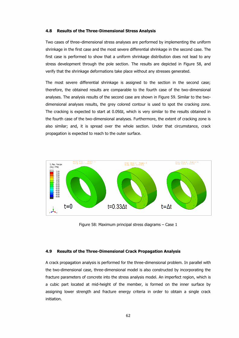
62
4.8 Results of the Three-Dimensional Stress Analysis
Two cases of three–dimensional stress analyses are performed by implementing the uniform
shrinkage in the first case and the most severe differential shrinkage in the second case. The
first case is performed to show that a uniform shrinkage distribution does not lead to any
stress development through the pole section. The results are depicted in Figure 58, and
verify that the shrinkage deformations take place without any stresses generated.
The most severe differential shrinkage is assigned to the section in the second case;
therefore, the obtained results are comparable to the fourth case of the two-dimensional
analyses. The analysis results of the second case are shown in Figure 59. Similar to the two-
dimensional analyses results, the grey colored contour is used to spot the cracking zone.
The cracking is expected to start at 0.09Δt, which is very similar to the results obtained in
the fourth case of the two-dimensional analyses. Furthermore, the extent of cracking zone is
also similar; and, it is spread over the whole section. Under that circumstance, crack
propagation is expected to reach to the outer surface.
Figure 58: Maximum principal stress diagrams – Case 1
4.9 Results of the Three-Dimensional Crack Propagation Analysis
A crack propagation analysis is performed for the three-dimensional problem. In parallel with
the two-dimensional case, three-dimensional model is also constructed by incorporating the
fracture parameters of concrete into the stress analysis model. An imperfect region, which is
a cubic part located at mid-height of the member, is formed on the inner surface by
assigning lower strength and fracture energy criteria in order to obtain a single crack
initiation.

63
Figure 59: Maximum principal stress diagrams – Case 2
The obtained results are presented in Figure 60 in terms of the level set contours. It can be
seen that the crack initiates from the defected point on the inner surface of the pole. The
initiation of cracking occurs at 0.02Δt. Cracking begins earlier than the estimation of stress
analysis due to the lower strength of imperfect zone. The initiated crack propagates in two
directions; the first direction is towards the outer surface and the second is along the
longitudinal dimension of pole. The three-dimensional crack surface is formed with
combination of propagation in these two directions; therefore, the complete longitudinal
crack geometry is obtained.
4.10 Discussion on Limitations of the Study
In this study, a time-dependent behavior of concrete and its effects on structural elements is
investigated. However, in the computational analyses the elastic properties of concrete,
which are also dependent on time, are considered to be constant for sake of simplicity. In
this case, the early-age tensile strength and modulus of elasticity of concrete are
overestimated. If these parameters were regarded as time-dependent parameters, then an
earlier crack initiation would be obtained in fracture analyses.
Another modeling assumption is the absence of lateral reinforcement. The plain concrete
material properties are assigned to the pole sections. As a matter of fact, usually spiral or
hoop steel is incorporated as lateral reinforcement against longitudinal cracking. This study
does not account for any lateral reinforcement, so considers the insufficiently reinforced
members.

64
Figure 60: Level set contours of three-dimensional crack propagation
Fig
ure
60:
Level se
t co
nto
urs
of
thre
e-d
imensi
onal cr
ack
pro
pagation

65
CHAPTER V
CONCLUSION AND RECOMMENDATIONS
Experimental studies of several researchers have revealed the cause of longitudinal cracking
problem encountered on spun-cast concrete poles. As per these studies, uneven shrinkage
of the segregated layers in a concrete pole cross-section results in severe durability
problems by means of cracking.
Based on the measurements presented in the experimental studies, two and three-
dimensional finite element models of segregated concrete pole have been constructed. The
obtained results of analyses have verified that the tensile strength of concrete is exceeded in
the inner layer of cross-section. It has been observed that the cracking zone extends from
the inner layer towards the outer layer as the gradient of the shrinkage increases over the
cross-section. A similar stress development is obtained by the three-dimensional analyses as
well.
The expected concrete fracture has been also modeled by use of XFEM, and a cracking
pattern, complying with experimental findings, is simulated. The analysis has shown that a
crack can propagate until it reaches the outer surface of the pole. In addition, effect of
reinforcements on crack propagation has been studied by a distinct model. The reinforced
model has revealed that crack propagation tends to go toward and terminate at a nearby
reinforced zone. This result is also concurrent with the findings of experimental studies.
Consequently, it can be concluded that the use of such computational tools may aid the
production process and the durability problems can be avoided by conducting a well-
designed production phase, thus eliminating segregation of the concrete. The computational
analyses have shown that a uniformly casted concrete pole will not suffer from excessive
tensile stress formation by uneven shrinkage.

66
For the future research, it would be interesting to include the diffusion-deformation
interaction into the problem to see its effect on the stress development and cracking. Also,
the reinforcement arrangement and the concrete cover thickness could be investigated to
reveal how they affect the crack initiation.
In this thesis study, the material properties are assigned as if concrete is homogeneous. A
more realistic and comprehensive study can be carried out by examining the mesostructure
of concrete through the pole section. By this means, it will become possible to assign
mechanical properties of constituents individually. Thus, more accurate crack propagation
analyses can be conducted.
The XFEM technique in ABAQUS version 6.10 has been used in this thesis study to
investigate a fracture problem. The obtained results have shown that XFEM is a reasonable
method to model fracture of concrete. Therefore, this method can be used to study the
nonlinear behavior of various structural concrete members.

67
REFERENCES
ABAQUS 6.10. “Abaqus Analysis User's Manual.” Dassault Systèmes, 2010.
ACI Committee 446. Fracture Mechanics of Concrete: Concepts, Models and Determination
of Material Properties. American Concrete Institute, 1991.
AFG-EL. Afghanistan Electric. 2012. Available from: http://www.afgel.com/ (cited March
2012).
Asferg, J. L. “Modeling of Concrete Fracture Applying the eXtended Finite Element Method.”
Ph.D. Thesis 2006.
Bazant, Z., P. "Concrete Fracture Models: Testing and Practice." Engineering Fracture
Mechanics, 2002: 165-205.
BelytschkoT., and T. Black. "Elastic Crack Growth in Finite Elements with Minimal
Remeshing." International Journal for Numerical Methods in Engineering, 1999: 601-
620.
Dilger, W. H., A. Ghali, and S. V. K. M. Rao. "Improving the Durability and Performance of
Spun-Cast Concrete Poles." PCI Journal, March/April 1996: 68-90.
Dilger, W. H., and S. V. K. M. Rao. "High Performance Concrete Mixtures for Spun-Cast
Concrete Poles." PCI Journal, July/August 1997: 82-96.
Dolbow J., Moës N., Belytschko T. "Discontinuous Enrichment in Finite Elements with a
Partition of Unity Method." Finite Elements in Analysis and Design, 2000: 235-260.
Fam, A. "Development of a Novel Pole Using Spun-Cast Concrete Inside Glass-Fiber-
Reinforced Polymer Tubes." PCI Journal, May/June 2008: 100-113.
Kudzys, A., and R. Kliukas. "The Resistance of Compressed Spun Concrete Members
Reinforced by High-Strength Steel Bars." Materials and Structures 41 (2008): 419-
430.
Mehta, P. K., and P. J. M. Monteiro. Concrete; Microstructure, Properties, and Materials. New
York: McGraw-Hill, 2006.
Moës N., Belytschko, T. "Extended Finite Element Method for Cohesive Crack Growth."
Engineering Fracture Mechanics, 2002: 813-833.
Mohammadi, S. Extended Finite Element Method: for Fracture Analysis of Structures.
Blackwell Publishing, 2008.
NavaChing. 04 24, 2008. http://www.navaching.com/ (accessed March 2012).
PCI, (Precast / Prestressed Concrete Institute). "Guide for the Design of Prestressed
Concrete Poles." PCI Journal, November/December 1997.

68
Rodgers, T. E. Jr. "Prestressed Concrete Poles: A State-of-the-Art Report." PCI Journal,
September/October 1984.
Shi, Z. Crack Analysis in Structural Concrete. Burlington: Elsevier, 2009.
Stolarska M., Chopp D. L., Moës N., Belytschko T. "Modelling Crack Growth by Level Sets in
the Extended Finite Element Method." International Journal for Numerical Methods
In Engineering, 2001: 943-960.
Turkish Standards Institution. "TS 500: Requirements for Design and Construction of
Reinforced Concrete Structures." 2000.
Zi G., Belytschko T. "New Crack-Tip Elements for XFEM and Applications to Cohesive
Cracks." International Journal for Numerical Methods in Engineering, 2003: 2221-
2240.