Part I. Rudiments

This part provides a rudimentary background of probability and statistical mechanics. It isexpected that the reader has already learned elementary probability theory and equilibriumstatistical mechanics. Therefore, it should be boring to repeat the usual elementary coursesfor these topic.

Chapter 1 outlines the measure-theoretical probability theory as intuitively as possible:the probability of an event is a ‘volume’ of our confidence in the occurrence of the event.Then, the most important law: the law of large numbers and its refinements, large devia-tion and central limit theorems are discussed. The law of large numbers makes statisticalthermodynamics possible, and large deviation theory gives the basis for most elementarynonequilibrium statistical mechanical approaches. Appendix outlines measure theory.

Chapter 2 is a review of the framework of equilibrium statistical mechanics along itshistory. It was born from kinetic theory. Elementary kinetic theory and the basic part ofBoltzmann’s kinetic theory are outlined. However, we are not interested in the theoreticalframework applicable only to special cases (dilute gases in this case). Therefore, kinetictheories are not discussed at length. Based on the expression of work (or equivalently themicroscopic expression of heat) due to Einstein, A = −kBT logZ is derived. Then, Jarzyn-ski’s equality is discussed. Eventually, we will learn that we have not yet understood thenature of the kind of motion we call heat. This is perhaps a major reason why we cannotunderstand nonequilibrium phenomena very well.

9

Chapter 1

Rudiments of Probability andStatistics

Almost surely the reader has already learned elementary probability theory. The purpose ofthis section is not to introduce elementary probability theory. We introduce the measure-theoretical probability as intuitively as possible. The reader should at least briefly reflecton what probability must be. Then, the three pillars of probability theory, crucial to statis-tical physics, are outlined in simple terms. They are the law of large numbers and its tworefinements, large deviation theory and central limit theorems. (Stochastic processes will bedefined in 1.4.2 but will be discussed later).

Their relevance to statistical physics is roughly as follows: the law of large numbersallows us to observe the reproducible macroscopic world (macroscopic phenomenology). Thelarge deviation theory tells us variational principles behind the macroscopic phenomenologyand fluctuations around the macroscopic results. Central limit theorems allow us to extractthe macroscopic picture of the world (= renormalization group theory).

Recommended reference of probability theory (for a second introduction):R Durrett, Probability: Theory and Examples (Wadsworth & Brooks Cole, Pacific Grove,Ca, 1991)1

1.1 Probability, an elementary review

Starting with a reflection on what ‘probability’ should be, we outline very intuitively thebasic idea of ‘measure theoretical probability.’ Appendix to this chapter is an introductionto measure theory.

The following book contains the most pedestrian introduction to measure-theoretical

1This is a role model of a textbook of any serious subject. However, it may not be the first book ofprobability the reader should read; it is a book for those who have firm basic knowledge.

10

probability theory I have ever encountered:Z. Brzezniak and T. Zastawniak, Basic Stochastic Processes — a course through exercises(Springer Verlag, 1999)

1.1.1 Probability as a confidence level.Probability of an event is a measure of our confidence (or conviction) level in 0-1 scale forthe event to happen.Discussion 1. Here, the word ‘confidence’ is used intuitively, but what is it? Your con-fidence must be tested. Your confidence must be useful, if you follow it. This means thatyour confidence must enhance your reproductive success. ut

Suppose there is a box containing white balls and red balls. The balls are all identicalexcept for the colors, and we cannot see inside the box. What is our confidence level ofpicking a red ball from the box? Our confidence level C in 0-1 scale must be a monotone in-creasing function of the percentage 100p% of red balls in the box. We expect on the averagewe pick a red ball once in 1/p picks (assuming that we return the ball after every pick andshake the box well; this is the conclusion of the law of large numbers →1.5.3). Therefore,C = p is a choice. That is, if one can repeat trials, the relative frequency of a success is agood measure of confidence in the success.

Let us consider another example. What do we mean, when we say that there will bea 70% chance of rain tomorrow? In this case, in contrast to the preceding example, wecannot repeat tomorrow again and again. However, the message at least means that theweather person has this much of confidence in the rain tomorrow. We could imagine thatshe looked up all the data of similar situations in the past, or that she did some extensivehydrodynamic calculation and the error bar suggested this confidence level, etc. Thus, evenin this case, essentially, an ensemble of days with similar conditions is conceivable, and therelative frequency gives us a measure of our confidence level.2

1.1.2 Probability is something like volume.If two events never occur simultaneously, we say these two events are mutually exclusive.3

For example, suppose a box contains white, red, and yellow balls. We assume that we cannotsee the inside of the box and the balls are identical except for their colors. Picking a red balland picking a yellow ball are two mutually exclusive events.

Suppose our confidence level of picking a red ball be CR and that for a yellow ball beCY . Then, what is our confidence level of picking a red or a yellow ball? It is sensible torequire that this confidence level is CR + CY . This is just in accordance with the choice‘C = p’ (or the additivity justifies that this choice is the best).Discussion 1. In the above it is said CR + CY is ‘sensible.’ Why or in what sense is itsensible? ut

This strongly suggests that our confidence level in 0-1 scale = probability is somethinglike a volume or weight of an object: if an object R has volume or weight WR and anotherobject Y weight WY , the weight of the nonoverlapping (= mutually exclusive) compoundobject made by joining R and Y must be WR +WY .

Our confidence level for an event that surely happens is one; for example, we can surelypick a ball irrespective of its color in the above box example, so, if CW is our confidence level

2In any case, the confidence level, if meaningful at all to our lives, must be empirically reasonable. Is thereany objective way to check the reasonableness of a confidence level without any use of a kind of ensemble?

3Do not confuse this with the concept of (statistical) independence (→1.2.2). If two events are (statisti-cally) independent, the occurrence of one does not tell us anything about the other event.

11

of picking a white ball, CR + CY + CW = 1. Thus, probability looks like volume or weightwhose total volume (weight or mass) is unity.

Suppose a shape is drawn in a square of area 1. If we pepper points on the squareuniformly, then the probability = our confidence level of a point to land on the shape shouldbe proportional to its area.4 Thus, again it is intuitively plausible that probability and areaor volume are closely related.Discussion 2. ‘Uniformly’ is a tricky word. The reader should have smelled a similardifficulty as encountered in the principle of equal probability in equilibrium statistical me-chanics (→2.6.2). Uniform with respect to what? Even if we could answer this question, isthe thing we base our uniformity really uniform (with respect to what?)? Critically thinkwhether we can really have objective ‘uniformity.’5 (For example, in Euclidean geometry theuniformity of the space must be assumed axiomatically. How is it done? Even if the readerscrutinizes Euclid, she will never find any relevant statement. That is, as is of course wellknown, Euclid’s axiomatic system is (grossly) incomplete.) ut

1.1.3 What is probability theory?A particular measure of the extent of confidence may be realistic or unrealistic (rational orirrational), but this is not the concern of probability theory. Probability theory studies thegeneral properties of the confidence level of an event.

The most crucial observation is that the confidence level behaves (mathematically orlogically) just as volume or weight as we have seen in 1.1.2. Let us write our confidence level= probability of event A as P (A). If two events A and B are mutually exclusive, P (A or Boccurs) = P (A) + P (B) (→1.1.5(2)). Such basic properties were first clearly recognized asaxioms of probability by Kolmogorov in 1933.6,7

1.1.4 Elementary and compound events.An event which cannot (or need not) be analyzed further into a combination of events iscalled an elementary event. For example, to rain tomorrow can be regarded as an elementaryevent, but to rain or to snow tomorrow is a combination of two elementary events, and iscalled a compound event.

Let us denote by Ω the totality of elementary events allowed under a given situation orto a system.8 Any event under consideration can be identified with a subset of Ω. Therefore,a subset of Ω is called an event. When we say an event A occurs, we mean that one of theelements in A occurs.

1.1.5 Definition of probability.Let us denote a probability of A ⊂ Ω by P (A). It is defined as a function whose domain is

4This has a practical consequence. See 1.5.6.5If the reader happens to know the so-called algorithmic probability theory, she may claim that there is

an objective definition of uniform distribution, but there all the symbols are assumed to be equally probable.6This year, Hitler was elected German Chancellor; Stalin began a massive purge; Roosvelt introduced

New Deal.7Kolmogorov’s work is a direct response to Hilbert’s address to the second International Congress of

Mathematicians in Paris held in 1900 (see “Mathematical problems,” Bull. AMS 8 437 (1992)). He namedprobability as one of the subdisciplines of physics whose axiomatic foundations needed investigation. Chapter2 of G. Shafer and V. Vovk, Probability and Finance, it’s only a game! (Wiley-Interscience 2001) is a goodsummary of the history of probability.

8That Ω is treated as a set is implicit here.

12

the totality of the sets in Ω,9 and whose range is [0, 1], satisfying the following conditions:(1) Since probability should measure the degree of our confidence on the 0-1 scale, we demandthat

P (Ω) = 1; (1.1.1)

in other words, something must happen. Then, it is also sensible to assume

P (∅) = 0. (1.1.2)

(2) Now, consider two mutually exclusive events, A and B. This means that whenever anelementary event in A occurs, no elementary event in B occurs and vice versa. That is,A ∩B = ∅. As we have already discussed, it is sensible to demand additivity

P (A ∪B) = P (A) + P (B), if A ∩B = ∅. (1.1.3)

It is convenient to require the additivity to infinitely many sets:(2’) [ σ-additivity ]: Suppose Ai (i = 1, 2, · · ·) are mutually exclusive events (Ai ∩Aj = ∅ forany i and j (6= i)). Then,

P (∪iAi) =∑i

P (Ai). (1.1.4)

In mathematical terms, probability P is a σ-additive measure with total weight unity. InAppendix to this Chapter, measure is explained informally; any statistical physicist shouldknow its rudiments.

(Ω, P ) is called a probability space.10

Note that for a given totality of elementary events Ω, there are many different proba-bilities just as there are many different unfair coins. For a coin Ω = H,T (head and tail),and P (H) = ph and P (T ) = 1− ph define a probability P .Exercise 1. There are 50 people in a room. What is the probability of finding at least twopersons sharing the same birthday? utExercise 2. There is a unit circle on which we wish to draw a chord whose length is longerthan

√3. What is the probability of drawing such a chord by randomly drawing it?11 [Notice

that the word ‘randomly’ is as tricky as ‘uniformly’ (→1.1.2)]. ut

1.1.6 On the interpretation of probabilityMathematicians and philosophers have been thinking about the interpretation of probability;as a branch of mathematics the measure theoretical framework may be enough, but to applyprobability to the real world some interpretation is needed.

There are two major camps in this respect: the frequentists vs. the ‘subjectivists’. Theformer asserts that probability is interpreted as relative frequency (out of an ensemble ofevents). The latter points out the difficulty in the interpretation of a unique event (an eventthat occurs only once, e.g., our lives), and asserts that some probabilities must be interpreteddeductively rather than inductively as the frequentists advocate.12

9Such a function is called a set-theoretical function; volume (→1.A.2) is an example. Not all the setshave volume; not all the events have probability. Therefore, precisely speaking, we must deal only the eventswhose probability is meaningful. See 1.A.20.

10This is not enough to specify a probability (→1.A.20), but we proceed naively here.11There is a very good account of this problem on p21-2 of N G van Kampen, Stochastic Processes in

Physics and Chemistry (North Holland, 1981). This is a nice book, but should be scanned quickly afterlearning the standard probability theory.

12Propensity interpretation by Popper, interpretation in terms of degree of confirmation by Carnap, etc.

13

Our starting point in 1.1.1 was probability = measure of confidence, so the reader mighthave thought that the lecturer was on the subjectivist side. However, this subjective measuremust agree at least to some extent with the actual experience in our lives. Thus, the rela-tion with relative frequency was immediately discussed there. The lecturer’s point of viewis that probability is a measure of confidence inductively supported by relative frequency.‘Non-frequentists’ forget that our mental faculty being used for deduction is a product ofevolution; our confidence may not be tied to our own experience, but is tied to the result ofour phylogenetic learning = the totality of experiences by our ancestors during the past 4billion years.13

Laplace is the founder of probability theory.14 His basic idea was: the relative numberof equally probable elementary events in a given event is the probability of the event. Here,‘equally probable’ implies that there is no reason to have difference. This is exactly theinterpretation of probability used by Boltzmann when he discussed entropy (→2.4.2).

If we feel that there is no reason to have difference between event A and event B, thenwe feel A and B are equally likely. This feeling is often in accordance with our experiencethanks to the evolution process that has molded us. That is, both our feeling and the ‘logic’behind Laplace’s and Boltzmann’s fundamental ideas have the basis supported by phyloge-netic learning.

Probability is always disguised relative frequency. Purely deductive probability conceptis meaningless.Discussion 1. Read the article by N. Williams, “Mendel’s demon” in Current Biology 11,R80-R81 (2001) and discuss the positive meaning of randomness.15

ut

1.2 Conditional Probability and Bayesian Statistics

1.2.1 Conditional probability: elementary definitionSuppose we know for sure that an elementary event in B has occurred. Under this condition

13Wittgenstein thought deeply on related problems. Let us read some passages of Philosophical Inves-tigations [There is a 50th anniversary commemorative edition: the German text with a revised Englishtranslation (by G. E. M. Anscombe), Third Edition; Blackwell, Oxford, 2001].“472. The character of the belief in the uniformity of nature can perhaps be seen most clearly in the case inwhich we fear what we expect. Nothing could induce me to put my hand into a flame — although after allit is only in the past that I have burnt myself.” (p114)“481. If anyone said that information about the past could not convince him that something would happenin the future, I should not understand him. One might ask him: What do you expect to be told, then? Whatsort of information do you call a ground for such a belief? What do you call “ conviction”? In what kind ofway do you expect to be convinced? —If these are not grounds, then what are grounds? — · · ·.” (p115)“483. A good ground is one that looks like this.” (p115)

14The Laplace demon that can predict everything deterministically was introduced to indicate its absurdityand to promote probabilistic ideas in the introduction to his Essai philosophique sur les probabilites (1814,this year Napoleon abdicated; Fraunhofer lines; Berzelius introduced the modern chemical symbols now inuse).

15This article is an introduction to the following book: M. Ridley, The Cooperative Gene— How Mendel’sDemon explains the evolution of complex beings (The Free Press, 2001), “Mendel’s demon is the executiveof gene justice, and we all depend on it for our existence.” Mendel’s demon is five years elder to Maxwell’sdemon.

14

what is the probability of the occurrence of another event A? This question leads us tothe concept of conditional probability. We write this conditional probability as P (A|B), anddefine it through

P (A ∩B) = P (A|B)P (B). (1.2.1)

1.2.2 IndependenceIf two events A and B satisfy

P (A ∩B) = P (A)P (B), (1.2.2)

these two events are said to be (statistically) independent.This definition is intuitively consistent with the definition of the conditional probability

in 1.2.1. If B has no information about A, then P (A|B) = P (A) is plausible. Thus, (1.2.1)reduces to (1.2.2).

Logically, we must define the independence of countably many events such as P (A∩B∩C) = P (A)P (B)P (C), because pairwise independence (1.2.2) does not imply such a relationamong many events as the reader sees in Exercise 1.Exercise 1.16 Let X1, X2 and X3 be independent random variables with P (Xi = 0) =P (Xi = 1) = 1/2. Consider the following three events: A1 = X2 = X3, A2 = X3 = X1and A3 = X1 = X2.(1) Show that these events are pairwisely independent.(2) P (A1 ∩ A2 ∩ A3) 6= P (A1)P (A2)P (A3).ut

Kolmogorov proved:There are infinitely many independent random variables on an appropriate probability space.

1.2.3 Borel-Cantelli lemmaLet A1, A2, · · · be an infinite sequence of events.(1) If

∑∞i=1 P (An) <∞, then with probability 1 only finitely many events among Ai occur.

(2) If all the events Ak are independent and if∑∞i=1 P (An) = ∞, then with probability 1

infinitely many of the events in Ai occur.[Demo] Here, a detailed (pedestrian) demonstration is given, because its logic is quite typical.(1) To demonstrate probabilistic statements, explicitly writing down the event or its comple-ment (negation) is often the best starting point. The negation of ‘only finitely many’ means‘infinitely many.’ If there occur infinitely many of Ak, for any n some Aj (j ≥ n) mustoccur. That is, Bn ≡ ∪j≥nAj must occur for any n. That is, all Bn must occur, or ∩n≥1Bn

must occur. Therefore, to demonstrate (1) we must show

P (∩n≥1 (∪j≥nAj)) = 0. (1.2.3)

This can be shown as follows:

P (∩n≥1 (∪j≥nAj)) ≤ limn→∞

P (∪j≥nAj) ≤ limn→∞

∑j≥n

P (Aj) = 0, (1.2.4)

because the series∑∞i=1 P (An) converges.

(2) Again, the negation is easier to prove: the probability of the occurrence of only finitely

16Taken from Durrett Example 4.1.

15

many of Ak is zero. If only finitely many of them occur, then all of Ω\Ak must occur for k ≥n for some n. That is, ∩k≥n(Ω\Ak) must occur for some n. That is, ∪n≥1 (∩k≥n(Ω \ Ak)) mustoccur. However, this is the negation of the statement we wish to demonstrate. Therefore,we wish to show that ∪n≥1 (∩k≥n(Ω \ Ak)) never occurs: we must show

P (∪n≥1 (∩k≥n(Ω \ Ak))) = 0. (1.2.5)

This can be demonstrated as follows:

P (∪n≥1 (∩k≥n(Ω \ Ak))) ≤ limn→∞

P (∩k≥n(Ω \ Ak)) = limn→∞

∏k≥n

P (Ω \ Ak). (1.2.6)

The last equality is due to the independence of all Ω \ Ak. Since∑k≥n P (Ak) diverges for

any n,∏k≥n(1− P (Ak)) = 0 for any n.17 This implies the product in (1.2.6) vanishes.

1.2.4 Conditional probability: mathematical comment(1.2.1) has no difficulty at all so long as we study a discrete probability space. However,there are many events that can change continuously. Suppose the event B is the event thata molecule in a cube of edge 1m has the speed infinitessimally close to 1m/s (event B). Thereader might say such an event is meaningless because it is ‘measure zero’ or probability zero.However, it is conceivable that the particle has such a speed and in a ball of radius 10cm inthe cube (event A). The conditional probability P (A|B) should be intuitively meaningful.

According to (1.2.1), it is 0/0, so its definition requires some care; since the ratioP (A∩B)/P (B) is 0/0, conceptually it is close to a derivative. Obviously, P (A∩B) < P (B),so this derivative is always well-defined. Such a derivative is called the Radon-Nikodymderivative. We will discuss this when we really need such sophistication.18

1.2.5 Bayes’ formulaSuppose we know the conditional probability P (x|θ) of X with the condition that Θ takesthe value θ. Then,

P (x, θ) = P (x|θ)P (θ) = P (θ|x)P (x). (1.2.7)

Therefore, we have

P (θ|x) =P (x|θ)P (θ)∑θ P (x|θ)P (θ)

. (1.2.8)

This is called Bayes’ formula.This formula is used, for example, as follows. Θ is a set of possible parameter values

that describe (or govern) the samples X we actually observe. Thus, P (x|θ) is the probabilitywe observe x, if the parameter value is θ. However, we do not know the actual θ. Fromthe actual empirical result we can estimate P (x|θ), assuming a model of the observation.Our aim is to estimate θ that is actually behind what we observe; you could interpret this

17A clever way to show this is to usee−x ≥ 1− x.

This impliese−∑

xk ≥∏

(1− xk).

18If you are impatient, A. N. Kolmogorov and S. V. Fomin, Introductory Real Analysis (Revised Englishedition, Englewood Cliffs,1970) is recommended.

16

as a problem selecting a model describing the observed phenomenon. A sensible idea is themaximum a posteriori probability estimation (MAP estimation): Choose θ that maximizeP (θ|x).

However, to use (1.2.8) we need P (θ): the a priori probability. The usual logic is thatif we do not know anything about Θ, P (θ) is uniform. Of course, this is a typical abuse ofOccam’s razor.19

1.2.6 Linear regression from Bayesian point of viewLet us assume that the independent variable values tk ((k = 1, · · · , N) are obtained withoutany error. For tk the observed dependent variable is yk but this is not without error:

yk = atk + b+ εk. (1.2.9)

The problem is to estimate a and b. In the resent problem εk are assumed to be iid20 Gaussianvariables with mean zero and variance V . Then, under the given parameters a, b

P (yk|a, b) =1

√2πV

N exp(− 1

2V

∑(yk − atk − b)2

). (1.2.10)

To use (1.2.8), we need P (a, b) the prior probability. If we assume that the prior is uniform,then the a posteriori probability is

P (a, b|yk) ∝1

√2πV

N exp(− 1

2V

∑(yk − atk − b)2

). (1.2.11)

Therefore, the MAP estimate dictates the least square scheme of determining a and b.

1.2.7 Problem of a priori probabilityBayesian statistics requires a priori probability. Sometimes, as have seen in 1.2.6, we coulddisregard it but the reason for ignoring the a priori probability is not very clear.

The reader must have thought about the principle of equal probability. This is the apriori distribution. Notice that the principle is made of two parts:(1) Designation of microstates (or elementary events).(2) Probability assignment to each elementary event.

In a certain sense, (1) is not a serious problem thanks to quantum mechanics. Sincevery high energy excitations cannot occur, we may totally ignore the structure of the worldat extremely small scales. Thus, Nature dictates what we may ignore.

However, (2) does not disappear even with quantum mechanics as already discussed.Thus, the problem of a priori distribution is a real issue.

If we wish to establish a general statistical framework for nonequilibrium states, (1)may well be the same as in equilibrium statistics. Thus, (2) becomes the key question ofnonequilibrium statistical mechanics.

19“Occam’s razor, in its legitimate application, operates as a logical principle about the complexity ofargument, not as an empirical claim that nature must be maximally simple. · · · Whereas Occam’s razorholds that we should not impose complexities upon nature from non-empirical sources of human argument,the factual phenomena of nature need not be maximally simple — and the Razor does not address thiscompletely different issue at all.” (S. J. Gould, The Structure of Evolution Theory (Harvard UP, 2002)p552). That is, questions about actual phenomena (e.g., whether two events are equally probable or not)should not invoke the razor. However, it seems empirically true that the abuse of the razor often works. Themost natural explanation is that our reasoning utilizes our brain, a product of natural selection.

20A standard abbreviation for “independently and identically distributed.”

17

1.3 Information

This section is not included in the ‘minimum’ to understand rudiments of nonequilibriumstatistical mechanics. Therefore, the reader could skip this section. However, it is a goodoccasion to have some familiarity to the topic. An excellent general introduction to the topicis:T. M. Cover and J. A. Thomas, Elements of Information Theory (Wiley, 1991)

1.3.1 Probability and informationSuppose there are two sets of symbols Ln and Lm that contain n and m symbols, respectively(n > m). Let us assume that all the symbols appear equally probably. Now, we just receivedtwo messages with 20 symbols. Which do we expect to have more information, the messagein symbols in Lm or that in Ln?

Here, the reader must ‘naively’ interpret the word ‘information.’ For example, comparethe English alphabet and the Chinese characters. We would certainly say 20 Chinese char-acters carry more information; with only 20 Chinese characters the world greatest poemswere written. Therefore, we expect the message written in the symbols in Ln should havemore information than that in Lm. Let us introduce (the average) information per symbolHn = H(Ln)

21 in the message written in the symbols in Ln as an increasing function of n.What we are trying to do now is this: it is very hard to characterize ‘information,’ so

let us at least try to quantify it, just as we do for energy. If the probability of encountering aparticular symbol (for Ln this is p = 1/n for any symbol) is small, the information carried bythe symbol is large. This is the fundamental relation between information and probability.

Now, let us use two sets of symbols Ln and Lm to send a message. We could makecompound symbols by juxtaposing them as ab for a ∈ Ln and b ∈ Lm (just as many Chinesecharacters do). The information carried by each compound symbol should be I(mn), be-cause there are mn symbols. To send the message written by these compound symbols, wecould send all the left half symbols first and then the right half symbols later. The amountof information sent by these methods must be equal, so we must conclude that

Hmn = Hm +Hn. (1.3.1)

Here, Hn is defined on positive integers n, but we can extend its definition to all positivereal numbers as

Hn = c log n, (1.3.2)

where c > 0 is a constant. Its choice is equivalent to the choice of unit of information andcorresponds to the choice of the base of the logarithm in the formula.

If c = 1 we say we measure information in nat; if we choose c = 1/ log 2, in bit. One bitis an amount of information obtained by the answer to a single yes-no question.Remark. However, we do not discuss the ‘value’ of information. ut

21In the notation H(Q), Q is a random variable, or a probability space.

18

1.3.2 Shannon’s information formulaAlthough we have assumed above that all the symbols are used evenly, such uniformity doesnot occur usually. What is the most sensible generalization of (1.3.2)?

A hint is already given in 1.3.1. If we write Hn = − log2(1/n) bits, − log2(1/n) is theexpectation value22 of information carried by a single symbol chosen from Ln. 1/n is theoccurrence probability of a particular symbol. Then, for the case with nonuniform occurrencep1, · · · , pn, the expectation value of the information carried by the i-th symbol should bedefined as − log2 pi bits. Therefore, the average information in bits carried by a single symboltaken from Ln should be defined by23

H(Ln) = −n∑i=1

pi log2 pi. (1.3.3)

This is called the Shannon information formula.24

− log2 pi is sometimes called the surprisal of symbol i, because it measures how muchwe are surprised by encountering this symbol. Expected surprisal is the information.Exercise 1.(1) Given a fair die, we are told that the face with 1 is up. What is the information inbit carried by this message? [The information of a message is measured by the change ofinformation (decrease of entropy, because often gain of information is equated with decreaseof entropy) one has due to the knowledge in the message.] (2.58 bits)(2) We are told that the sum of the faces of two fair dice is 7. What is the informationcarried by this message? (2 × 2.58 − 2.58 = 2.58 bits). utExercise 2. Suppose we have a sentence consisting of 100 letters. We know that the infor-mation per letter is 0.7 bit. How many ye-no question s do you need to completely determinethe sentence? utDiscussion 1. If the symbols of English alphabet (+ blank) appear equally probably, whatis the information carried by a single symbol? (4.58 bits) In actual English sentences, it isabout 1.5(?) bits. What happens? Also think about how to determine this actual value.25,26

ut

1.3.3 Information for continuous distributionLet f be the density distribution function on an event space (probability space) that iscontinuous. It is customary to define the Shannon entropy of this distribution as

H = −∫dx f(x) log f(x). (1.3.4)

This formula was originally introduced by Gibbs as we see in 2.1.5.Warning. Notice that the formula has a very serious defect. The formula is not invari-ant under the coordinate transformation. Further worse, it is not invariant even under the

22Here, ‘expectation value’ may be understood intuitively and in an elementary way, but for a moremathematical definition see 1.4.3.

23Notice that the symbol set is actually a probability space (Ln, pj).24for an uncorrelated (or Bernoulli) information source. About Shannon himself, see S. W. Golomb et al.,

“Claude Elwood Shannon (1916-2002),” Notices AMS 49, 8 (2002), and J. F. Crow, “Shannon’s brief forayinto genetics,” Genetics 159, 915 (2001).

25Cf. Cover and Thomas, Chapter 6 “Gambling and Data Compression.”26There is a related ‘fun’ paper, Benedetto et al., “Language tree and zipping,” Phys. Rev. Lett. 88,

048702-1 (2002). This uses Lempel-Ziv algorithm LZ77 (used in gzip, for example) to measure information(or rather mutual information).

19

change of the unit to measure the coordinates, because the scaling transformation of theindependent variable x → αx alters the value of H. Generally speaking, no dimensionfulquantity should appear inside the logarithmic function. ut

The reader must have realized that f inside the logarithm should be a ratio. See 1.6.9.In short, (1.3.4) may be used only under the assumption that x is a priori equally weighted.

1.3.4 Information and entropyH(A) is the expected information we obtain from one sample from A. The information shecan gain on the average from the answer that the symbol is a particular one is given by H(A).Thus, as we have already seen in Exercise 2 in 1.3.2, if we obtain nH(A) information, wecan determine a sentence sn made of n symbols taken from A.27

Suppose we already know the sentence sn. Then, there is no surprise at all, even ifwe are shown sn: the information carried by sn is zero. This means that the informationnH(A) has reduced our ignorance from the initial high level to the final perfectly informedlevel. A convenient measure of the extent of ignorance is entropy in equilibrium statisticalmechanics. Therefore, we could say that nH(A) of information has reduced the entropy tozero. It is sensible to guess that the initial entropy is nH(A). This is the Gibbs-Shannonentropy-information relation seen in (1.3.3) or (1.3.4).

Thus, information and entropy are often used interchangeably. If there is a macroscopicstate whose entropy is S, to specify a single microstate (= elementary event) we need (onthe average) information H = S.Exercise 1. When reaction occurs, the entropy of the reacting chemicals change. This isusually measured in en (entropy unit) = cal/mol·K. How many bits per molecule does 1 encorrespond? Is the reader’s answer reasonable?28 How about in pNnm/K?29 utDiscussion 1. How much energy is required to transfer 1 bit between two communicators?30

ut

1.3.5 Information minimization principleLet us consider the problem of estimating the ‘most likely’ distribution (density distribution

27On the average. However, if n is very large, the accuracy (= density of correctly identified letters)asymptotically reaches unity.

28If the entropy is measured in eu as S eu, then it is 0.72S bits/molecule.29

kB = 1.381× 10−23 J/K,= 1.381× 10−2 pN · nm/K,= 8.617× 10−5 eV/K

The gas constant R is given by

R ≡ NAkB = 8.314 J/mol ·K = 1.986 cal/mol ·K (1.3.5)

Here, 1 cal = 4.18605 J. It is convenient to remember that at room temperature (300K)

kBT = 4.14 pN · nm= 0.026 eV

RT = 0.6 kcal/mol.

30R Landauer, “Energy requirements in communication,” Appl. Phys. Lett. 51, 2056-2059 (1987).

20

function) of a variable describing a system under some known conditions or knowledges, say,the average and the variance.

To answer this question we must interpret the requirement ‘most probable’ appropri-ately. One interpretation is that the most probable distribution is the one with the leastbiased under the extra conditions or knowledges we are at hand. A quantitative version ofthis interpretation uses the Shannon information as follows.

Compare the a priori distribution and the distribution we can infer with the extra knowl-edge. The most unbiased distribution we should infer must correspond to the distributionof the symbols with the least decrease of information per symbol compatible with the extracondition. Therefore, the distribution we wish to infer must be obtained by the maximizationof the Shannon formula (1.3.4) or (1.3.3) under the extra conditions imposed. The decreasein H may be interpreted as the information gained from the extra conditions. Therefore, theprescription is to minimize the information gain from the newly acquired conditions. Thisis the so-called Jaynes’ principle. The principle is useful, if we do not stretch it, or if we useit as a shortcut to known results.

The astute reader should have already realized that the principle works only when weknow that the a priori distribution is uniform (= the principle of equal probability). Fur-thermore, from the warning in 1.3.3, if the event is described by continuous variables, afurther caution is required to use this principle. A typical abuse is the ‘derivation of statis-tical mechanics’ 1.3.6.Discussion 1. The distribution available by the information minimization principle and thetrue distribution are very likely different under nonequilibrium conditions.31 ut

1.3.6 Information-theoretical foundation of statistical mechanics is illusory.The information H is maximized when all the symbols (or events) occur equally probably.Some people wish to utilize this property to justify (or derive) the principle of equal proba-bility (→2.6.2) (the so-called information theoretical foundation of statistical mechanics32).

Let us maximize (1.3.3) under the condition that we know the expectation value ofenergy

∑Eipi = E.

Exercise 1. Using Lagrange’s multipliers, find pi in terms of Ei. utAs the reader has seen, the canonical distribution

pi ∝ e−βEi (1.3.6)

is obtained, where β is determined to give the correct expectation value of the energy.33

The logic is that H measures the amount of the lack of our knowledge, so this is the mostunbiased distribution (→1.3.5). ut

But does Nature care for what we know? Even if She does, why do we have to chooseShannon’s information formula to measure the amount of our knowledge?

The formula (1.3.3) is so chosen that if all the symbols appear equally probably, thenit depends only on the total number of elements (→1.3.1). Therefore, logically, there is avicious circle. The reader will encounter a similar quantity, the Kullback-Leibler entropylater (→1.6.9), and will clearly recognize the fundamental logical defect in the so-called

31For example, see a recent paper: H.-D. Kim and H. Hayakawa, “Test of Information Theory on theBoltzmann Equation,” J. Phys. Soc. Japan, 72 2473 (2003).

32E T Jaynes, Phys. Rev. 106, 620 (1959).33Boltzmann’s argument summarized in Exercise of 2.4.11 just derives Shannon’s formula and uses it. A

major lesson is that before we use the Shannon formula important physics is over. The reader can use theShannon formula as a shortcut, but can never use it to justify what she does.

21

information theoretical foundation of statistical mechanics.Exercise 2. Is (1.3.6) really correct? [Suppose we do not know what the elementary event isin statistical mechanics and (erroneously) assume that elementary states are defined by theirenergy (that is, however many microstates we have for a given energy, they are assumed tobe a single state).] utExercise 3. The use of the least square fit assumes that the error obeys a Gaussian dis-tribution. Suppose we wish to fit the data g(s) (s ∈ [0, 1]) with a function f(s, α) with aparameter, choosing the parameter through minimizing the “L2-error”:∫ 1

0ds|g(s)− f(s, α)|2. (1.3.7)

We could also use an appropriate function M and minimize∫ 1

0ds|M(g(s))−M(f(s, α))|2. (1.3.8)

Show that the answers cannot generally be identical. utThe reader must clearly recognize that information theory can never be used to justify

or derive any fundamental statistical hypothesis.

1.3.7 Joint entropy and conditional entropyLet X = x1, · · · , xn and Y = y1, · · · , ym be the letter sets. If p(x, y) is the probabilityfor a pair of letters x, y (x ∈ X, y ∈ Y ).

H(X, Y ) = −∑

x∈X,y∈Yp(x, y) log p(x, y) (1.3.9)

is the joint entropy of X and Y .Consider H(X, Y )−H(X). This must be the information (per letter pair) we can gain

from x, y, when we already know x, Therefore, this is called the conditional entropy of Y .Thus, the following is a reasonable definition of the conditional entropy:

H(Y |X) = H(X, Y )−H(X) (1.3.10)

Notice that

H(Y |X) = −∑x,y

p(x, y) log p(x, y) +∑x

p(x) log p(x), (1.3.11)

= −∑x,y

p(x, y) log p(x, y) +∑x,y

p(x, y) log p(x), (1.3.12)

= −∑x,y

p(x, y) log p(y|x) =∑x

p(x)

[−∑x,y

p(y|x) log p(y|x)]. (1.3.13)

Here, p(y|x) is the conditional probability of y under condition x. If we introduce

H(Y |x) = −∑y

p(y|x) log p(y|x), (1.3.14)

we can writeH(Y |X) =

∑x

p(x)H(Y |x). (1.3.15)

22

We can writeH(X, Y ) = H(X) +H(Y |X). (1.3.16)

This is sometimes called the chain rule. For example,

H(X, Y, Z) = H(Y, Z) +H(X|Y, Z) = H(Z) +H(Y |Z) +H(X|Y, Z). (1.3.17)

It should be intuitively obvious that

H(X|Y ) ≤ H(X). (1.3.18)

This can be shown algebraically with the aid of the log sum inequality.

1.3.8 Log sum inequalityFor non-negative numbers a1, · · · , an and b1, · · · , bn

n∑i=1

ai logaibi≥(

n∑i=1

ai

)log

∑ni=1 ai∑ni=1 bi

(1.3.19)

with equality iff ai/bi is constant.[Demo] Let f(t) = t log t. The Jensen34 implies for a stochastic vector α∑

αif(ti) ≥ f(∑

αiti). (1.3.20)

Now, set ti = ai/bi and αi = bi/∑bi. ut

1.3.9 Mutual informationThe mutual information I(X, Y ) between X and Y is defined as

I(X, Y ) = H(X) +H(Y )−H(X, Y ) =∑x,y

p(x, y) logp(x, y)

p(x)p(y). (1.3.21)

Obviously, this is symmetric. Intuitively, this must be positive, because non-independenceof X and Y should reduce the information that could have been carried by independent Xand Y .Exercise 1. Demonstrate that I(X, Y ) ≥ 0. ut

1.3.10 Asymptotic equipartition propertyLet Xi be iid variables with probability p(x). Then, in probability

− 1

nlogP (X1, · · · , Xn)→ H(X). (1.3.22)

This is just the weak law of large numbers (→1.5.4).

34If f is a convex function, 〈f(x)〉 ≥ f(〈x〉) (Jensen’s inequality).

23

1.3.11 Typical set of sequencesThe typical set A(n)

ε wrt p(x) is the set of xini=1 such that

2−nH−nε ≤ p(xi) ≤ 2−nH+nε (1.3.23)

for small positive ε.(1) If xi ∈ A(n)

ε , then H − ε ≤ −(1/n) log p(xi) ≤ H + ε.(2) For sufficiently large n P (A(n)

e ) ≥ 1− ε. That is, the typical set is almost probability 1.(3)

(1− ε)2nH−ε ≤ |A(n)ε | ≤ 2nH+ε. (1.3.24)

Here | | denotes the cardinality of the set. The number of typical elements is 2nH and theyare all equally probable.[Demo] (1) is the definition itself. For any δ > 0, there is an N such that ∀n > N

P(∣∣∣∣− 1

nlog p(xi)−H(X)

∣∣∣∣ < ε)> 1− δ. (1.3.25)

This is asymptotic equipartition or weak law of large numbers. We may set δ = ε. This is(2). Since

1 =∑

p(xi) ≤∑

q∈A(n)ε

p(q) ≤∑

q∈A(n)ε

2−nH−nε = |A(n)ε |2−nH−nε, (1.3.26)

we obtain the upper bound in (3). From (2)

1− ε < P (A(n)ε ) ≤

∑q∈A(n)

ε

2−nH+nε = |A(n)ε |2−nH+nε (1.3.27)

we obtain the lower bound.ut

1.3.12 Implication of typical set1.3.11 implies (roughly):If we produce uncorrelated sequences35 of n ( 1 in practice) letters with entropy H, thenonly 2nH of them appear. This typical set is usually vastly smaller than the totality of thepossible sentences and can be written in nH 0 and 1’s.

This is the principle of data compression,36 and is fully used in, e.g., jpeg. Of course,occasionally sentences not in the typical set show up. In such cases we simply accept thesituation as an unfortunate case and send or store such exceptional sequences as they arewithout compression. In any case, they are asymptotically very rare.

1.3.13 Statistical mechanics and law of large numbers revisitedThe fourth law of thermodynamics implies that a macroscopic system may be understoodas a collection of statistically independent macroscopic subsystems. The states of each sub-system may be characterized by the set of states of subsystems xi. We know with almostprobability one what we observe is from the asymptotic equiprobability states. Therefore,almost all the states of a macroscopic system have the same probability. This is an expla-nation of the principle of equal probability.

Thus, essentially the law of large numbers and the fourth law of thermodynamics areexpected to be the two key elements of statistical mechanics.

Then, what is the role of mechanics?

35If there are correlations, we could exploit it to convert the original sentences shorter.36A good exposition (not introductory) can be found in D. L. Donoho, M. Vetterli, R. A. DeVore, and I.

Daubechies, “Data Compression and Harmonic Analysis,” IEEE Transactions on Information Theory, 44,2435 (1998).

24

1.4 Random Variables

Basic tools such as characteristic functions, generating functions, etc., are introduced. Thereader must be familiar with an elementary technique to compute probability densities usingthe δ-function (→1.4.5).

1.4.1 Random variablesLet P be a probability (= probability measure →1.1.5) defined on a set Ω = totality ofelementary events under consideration.37 A function defined on Ω is called a random vari-able.38 A point in Ω (i.e., an elementary event) is often specified by a parameter ω calledthe stochastic parameter. Thus, a random variable can be written as f(ω).

Two random variables X and Y are said to be independent, if for any two real valuesets A and B39

P (X ∈ A ∩ Y ∈ B) = P (X ∈ A)P (Y ∈ B). (1.4.1)

1.4.2 Stochastic parameter and stochastic processRoughly speaking, a stochastic process is a function of time parameterized by a stochasticparameter. That is, a stochastic process is a functional on a probability space: a map froma probability space to a space of functions of time. Analogously, we can define a stochasticfield as a map from a probability space to a function defined on a space. ω specifies eachsample = a particular realization.

1.4.3 Expectation valueLet X(w) be a random variable on Ω and µ a probability on it 40. The expectation valueE[f ] of the random variable f is defined as

E(X) =∫ΩX(ω)dµ(ω). (1.4.2)

For a set (= event) A ⊂ Ω, the following function χA is called its indicator (or indicatorfunction):

χA(ω) =

1 ω ∈ A,0 ω 6∈ A. (1.4.3)

That is, the indicator for an event A is 1, if the event occurs, and 0, otherwise.The probability of an event A ⊂ Ω is µ(A), so

µ(A) =∫ΩχA(ω)dµ(ω) = E(χA). (1.4.4)

37As seen in Appendix to this chapter, not all the events have their probabilities (measurable), so we mustalso specify a family of measurable events = the events whose probability we can discuss, but we will notexplicitly write the so-called ‘triplet’ (→1.A.20).

38Again, we must discuss functions whose expectation values are meaningful, so we must require thatrandom variables must be P -measurable (→2.8.6). However, we will not explicitly write such a condition.

39A,B ⊂ R, but again not all the sets are measurable (have lengths), so we need some disclaimer here;we omit it as usual.

40We say X(ω) is a random variable on the probability space (Ω, µ).

25

That is, the expectation value of the indicator of an event is the probability of the event.If Ω is a discrete set, then the above integral reduces to an appropriate summation.E((X − E(X))n), if exists, is called the n-th moment (around the mean). The second

moment around the mean is called the variance and is often denoted as

V (X) ≡ E((X − E(X))2) = E(X2)− E(X)2. (1.4.5)

A necessary and sufficient condition for two square-integrable random variables (i.e.,random variables having the second moments) X and Y to be independent is: for anybounded functions41 f and g

E(f(X)g(Y )) = E(f(X))E(g(Y )). (1.4.6)

That is, we can average independent variables separately. utExercise 1. If X and Y have second moments, and are independent,

V (X + Y ) = V (X) + V (Y ). (1.4.7)

ut

1.4.4 Distribution functionsLet X(ω) be a real valued random variable.42

F (x) = P (X(ω) ≤ x) (1.4.8)

is called the probability distribution function for X. If we can write

f(x)dx = F (x+ dx)− F (x), (1.4.9)

f is called the probability density distribution function.43 Thus, f(x)dx = P (X(ω) ∈(x, x+ dx]).

If a function F on R satisfies:(i) F is non-decreasing,(ii) limx→−∞ F (x) = 0 and limx→∞ F (x) = 1,(iii) F is right continuous, i.e., limx→a+0 F (x) = F (a),F is a distribution function of a random variable.Exercise 1. The Cauchy distribution whose density is proportional to 1/(x2 + a2) does nothave the second moment.utExercise 2. “If n-th moment does not exit, m(> n)-th moments do not exist, either.” Isthis statement correct? ut

1.4.5 How to compute densityWe have

P (A) = E(χA), (1.4.10)

41Again, we omit the measurability condition.42Often the probability space is implicit.43The Radon-Nikodym derivative of F with respect to the Lebesgue measure is called, if exists, the

probability density function.

26

where χA is the indicator of A. If A ∈ Rn, we can write

χA(x) =∫Aδ(x− y) dny, (1.4.11)

where δ is the (n-dimensional) δ-function.For physicists the density distribution is often more familiar with than distributions:

the density distribution function f(x) of a random variable X is given by

f(x) = E(δ(X(ω)− x)). (1.4.12)

There are two major methods to compute this expectation. One is to use Fourier trans-formation which is equivalent to computing characteristic functions (→1.4.7). The other isto compute the integral directly. A typical problem is: Obtain the density distribution ψ(y)of y = g(x), given the density distribution of ρ(x) of x. This is to compute

ψ(y) = E(δ(g(x)− y)) =∫dx ρ(x) δ(g(x)− y) =

∑xi

ρ(xi)

|g′(xi)|, (1.4.13)

where g(xi) = y (the sum is over all real zeros of g − y) (→1.4.6).An example follows:

Suppose x is uniformly distributed on [−1/2, 1/2]. Find the density distribution functionψ(y) of y = x2. We obtain for y ∈ (0, 1/4]

ψ(y) =∫ 1/2

−1/2dx δ(y − x2) =

1√y. (1.4.14)

Exercise 1. Derive the energy density distribution function of a d-dimensional ideal gas inequilibrium. utExercise 2. Suppose x is distributed uniformly on [0, 1]. Let F (x) be a monotone increas-ing smooth function from R to [0, 1]. Find the density distribution φ of F−1(x) (the inversefunction of F ). utThe result of this exercise is a standard method to convert uniform random number on [0, 1]into the random number whose distribution function is given by F .

1.4.6 Computation of δ-function of complicated variableTo compute E(δ(g(x)− y)), the basic formula we use is

δ(g(x)− y) =∑xi

1

|g′(xi)|δ(x− xi), (1.4.15)

where g(xi) = y (the sum is over all real zeros of g − y).Let us demonstrate (1.4.15). The delta function does not contribute anything to the

integral, if its variable is not zero, so we have only to pay attention to the values of x thatgive zero of g(x)− y. Let x1 satisfy g(x1) = y. Then,

g(x)− y = g′(x1)(x− x1) + · · · . (1.4.16)

We must recall that δ(ax) = (1/|a|)δ(x). Therefore, the contribution from x near x1 must be(1/|g′(x1)|)δ(x− x1). There are other zeros as well. We should sum up all the contributionsfrom the zeros of g − y. This outcome is (1.4.15).

27

1.4.7 Characteristic FunctionThe Fourier transform of a probability measure µ is called its characteristic function:

ϕµ(ξ) ≡∫eiξxµ(dx). (1.4.17)

For a random variable X, the characteristic function of its distribution = probabilitymeasure µX is denoted by ϕX . The most important and useful property of this function is:If X and Y are independent random variables (cf. 1.4.1),

ϕX+Y (ξ) = ϕX(ξ)ϕY (ξ). (1.4.18)

Exercise 1.(1) Find the characteristic function of the Gaussian distribution N(m,V ) (with mean m andvariance V ).(2) Find the characteristic function of the n-dimensional Gaussian distribution with meanm and covariance matrix V .(3) Find the characteristic function of the Poisson distribution with average λ (i.e., µ(k) =(λk/k!)e−λ).(4) Find the characteristic function of the Cauchy distribution whose density is given by1/π(1 + x2). utExercise 2.(1) Find the characteristic function of the binary distribution (for k ∈ 0, 1, · · · , n)

µ(k) =

(n

k

)pk(1− p)n−k. (1.4.19)

(2) Let λ = np, and take the limit n→∞, p→ 0 with fixed λ. The outcome is the charac-teristic function of the Poisson distribution just discussed (cf. ??). ut

1.4.8 Properties of characteristic functionsThe characteristic function of a distribution is positive definite, i.e., for any positive integern, any complex numbers zjnj=1 and real numbers ξjnj=1

n∑j,k=1

zjzkϕµ(ξj − ξk) ≥ 0. (1.4.20)

It is clear thatϕµ(0) = 1. (1.4.21)

Also ϕ is continuous at the origin.44 The converse is also true (→1.4.9), so these threeproperties characterize the characteristic function.

If it is sufficiently smooth, we can compute moments (around the origin) by differenti-ating it:

E(Xn) = (−i)n dn

dξnϕX(ξ)

∣∣∣∣∣ξ=0

. (1.4.22)

44due to an elementary theorem of Lebesgue integration.

28

1.4.9 Bochner’s theorem.A positive definite function (in the sense of 1.4.8) ϕ on Rn that is continuous at the originand ϕ(0) = 1 is a characteristic function of some probability measure on Rn.ut

However, it is not always easy to check that a given function can be a characteristicfunction of a certain distribution. If φ is an even function, convex on (0,∞), and φ(0) = 1,then φ is a characteristic function (Polya’s criterion;45 note that this criterion cannot beapplied to the Gaussian case). For example, exp(−|ξ|α) for α ∈ [0, 1] is a characteristicfunction.Exercise 1. Let x(t, ω) be a continuous stochastic process (x(t, ω) is continuous foralmost all ω as a function of t), and 〈x(0, ω)2〉ω = 1. Also, let us assume that it is stationary(i.e., various expectation values do not depend on the absolute time). Demonstrate that itscorrelation function

C(t) = 〈x(t, ω)x(0, ω)〉ω (1.4.23)

is a characteristic function of a probability distribution. This is related to an importanttopic of spectral analysis of stochastic processes (→??) ut

1.4.10 Laplace transformation and generating functionThe Laplace transform of the measure µ, if exists,

Z(λ) =∫µ(dx)eλx (1.4.24)

is called the generating function of µ, and λ is its parameter. It may be more appropriateto call it the partition function.

Just as we have done for the characteristic function (→1.4.8), we can compute momentswith the aid of differentiation wrt λ. Its logarithmic differentiation is useful as the readerexpects from Gibbs’ work (→2.1.4). For example,

dlogZ

dlam

∣∣∣∣∣λ=0

= 〈x〉. (1.4.25)

Here (and henceforth), 〈 〉 implies the expectation value (averaging). In the case of canonicaldistribution we do not set λ = 0. We also have

d2 logZ

dλ2

∣∣∣∣∣λ=0

= 〈(x− 〈x〉)2〉. (1.4.26)

1.4.11 Cumulant expansionThe derivatives of the generating function at the origin of the parameter (→1.4.10) suggestthat the Taylor expansion of logZ(lam) around λ = 0 would give useful quantities. This is the idea of cumulant expansion:

logZ(lam) = λC1 +1

2λ2C2 + · · ·+ 1

n!λnCn + · · · , (1.4.27)

45Durrett p87.

29

where Cn is called the n-th cumulant, and is very often written as

Cn = 〈Xn〉C . (1.4.28)

It is easy to see that C1 = E(X), and C2 = V (X).With the aid of this notation (1.4.27) is succinctly rewritten (symbolically) as

logZ(λ) =⟨eλX − 1

⟩C

(1.4.29)

With the aid of log(1 +x) = −∑(−1)nxn/n and the multinomial expansion, cumulantsare related to the ordinary moments 〈Xn〉 (around the origin) as

〈Xn〉C = −n!∑

K·N=n

(K · 1− 1)!(−1)K·1 1

K!

(〈XN 〉N !

)K

. (1.4.30)

Here, N is a nonnegative integer vector N = (N1, N2, · · ·) such that N1 ≥ N2 ≥ · · · ≥ 0(of various dimensions), and the summation is over all possible choices of K = (k1, k2, · · ·),where ki specifies the number of Ni (i.e., the summation is over all the possible partition ofn). 1 = (1, 1, · · ·). (Slightly extended) Hadamard’s notation is adopted: for a vector A =

(a1, a2, · · ·), A! =∏ai!, xA =

∏xaii ; xA = (xa1 , xa2 , · · ·); A/N ! = (a1/N1!, a2/N2!, · · ·).

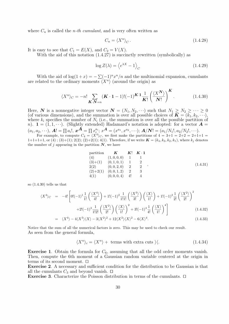
For example, to compute C4 = 〈X4〉C , we first make the partitions of 4 = 3+1 = 2+2 = 2+1+1 =1+1+1+1, or (4) ; (3)+(1); 2(2); (2)+2(1); 4(1). Therefore, if we write K = (k4, k3, k2, k1), where kj denotesthe number of j appearing in the partition N , we have

partition K K! K · 1(4) (1, 0, 0, 0) 1 1(3)+(1) (0, 1, 0, 1) 1 22(2) (0, 0, 2, 0) 2 2(2)+2(1) (0, 0, 1, 2) 2 34(1) (0, 0, 0, 4) 4! 4

, (1.4.31)

so (1.4.30) tells us that

〈X4〉C = −4!

[0!(−1)1

11!

(〈X4〉

4!

)+ 1!(−1)2

11!1!

(〈X3〉

3!

)(〈X〉1!

)+ 1!(−1)2

12!

(〈X2〉

2!

)2

+2!(−1)31

1!2!

(〈X2〉

2!

)(〈X〉1!

)2

+ 3!(−1)414!

(〈X〉1!

)4]

(1.4.32)

= 〈X4〉 − 4〈X3〉〈X〉 − 3〈X2〉2 + 12〈X2〉〈X〉2 − 6〈X〉4. (1.4.33)

Notice that the sum of all the numerical factors is zero. This may be used to check our result.As seen from the general formula,

〈Xn〉c = 〈Xn〉+ terms with extra cuts 〉〈. (1.4.34)

Exercise 1. Obtain the formula for C6, assuming that all the odd order moments vanish.Then, compute the 6th moment of a Gaussian random variable centered at the origin interms of its second moment. utExercise 2. A necessary and sufficient condition for the distribution to be Gaussian is thatall the cumulants C3 and beyond vanish. utExercise 3. Characterize the Poisson distribution in terms of the cumulants. ut

30

1.4.12 Gibbs-Helmholtz relation and generating functionThe internal energy is identified with (or is interpreted as) the average 〈H〉 of the Hamiltonianover the distribution P on the phase space (cf. 2.5.3). Then, the Gibbs-Helmholtz relation

E =∂(A/T )

∂(1/T )

∣∣∣∣∣V

= − ∂(−A/kBT )

∂(1/kBT )

∣∣∣∣∣V

, (1.4.35)

where A is the Helmholtz free energy, may be interpreted as: −A/kBT is the logarithm ofthe generating function of energy Z called the canonical partition function (→2.1.5),46 andβ = 1/kBT is the parameter of the generating function:

Z = e−βA =∑

e−βεw(ε), (1.4.36)

where w(ε) is the statistical weight of the states with energy ε and the sum is over possibleenergies. What Gibbs demonstrated (→2.1.4) is that if w(E)dE is the phase volume of theconstant energy shell between the energy surfaces with energy E and E + dE, then indeedA satisfies the ordinary thermodynamic relation thanks to Liouville’s theorem (→2.7.2).

However, as we have already seen, there is no way to impose this condition based onmechanics. Thus, a needed extra assumption is the principle of equal probability (→2.6.2)which is equivalent to the requirement that w(E)dE is the phase volume of the energy shellbetween energy E and E + dE.

1.5 Law of Large Numbers and Ergodic Theorem

THE Law of large numbers is the most important theorem of probability theory for statisticalmechanics. If we do not pay any attention to fluctuations, this (and Chebyshev’s inequality1.5.5) is the only probability theory we need to understand macroscopic systems. MonteCarlo methods (→1.5.6) are direct application of this theorem. Ergodic theorems (→1.5.8)may be interpreted as its generalization to correlated variables.

1.5.1 Law of large numbers: an illustrationLet Xi be 1 if the i-th coin tossing of a fair coin gives a head, and 0, otherwise. Sn =

∑ni=1Xi

implies the number of heads we get with n tossing experiments. Then, everybody knowsthat surely

Sn/n→ 1/2 (1.5.1)

as n → ∞. Here, Sn/n is called the sample mean or empirical average. This ‘law of largenumbers’ was first recognized by Jacob Bernoulli (1645-1705).47

46However, we do not set β = 0 after differentiation.47The statement given here is much stronger than Bernoulli’s version. His law is the weak law. That

is, if n is large enough, then the average deviation of Sn/n from m becomes less and less (→ 0). Thisstatement does not guarantee that for almost all the sample sequence Sn/n converges to m (for a particularsample sequence Sn/n may occasionally become big). What we intuitively know is that for almost all samplesequences Sn/n→ m. This is the strong law (→1.5.4 footnote).

31

Discussion 1. Make an example of A stochastic sequence such that P (|An| > 0) → 0,but An → 0 never holds. The existence of such a sequence implies that the meaning of theconvergence (1.5.1) is delicate. utExercise 1. For a finite n Sn/n is not exactly equal to 1/2 (that is, it is also a randomvariable), but fluctuates around it. Sketch the probability density distribution function forSn/n for several n, say, 100, 10,000, and 1,000,000.utFrom this exercise, the reader should have realized that the density distribution functionof Sn/n seems to converge to δ(x − 1/2), that is, the distribution converges to an atomicmeasure concentrated at x = 1/2.

1.5.2 Law of large numbers for iid random variablesLet Xi be a sequence of random numbers identically and independently distributed (iidis the standard abbreviation) on a probability space. Let us assume that E(X1) = m andV (X1) = C(<∞). The law of large numbers tells us

Sn/n→ m (1.5.2)

in a certain sense. As the reader expects, there are different ways to interpret this limit.Accordingly, there are different versions of law of large numbers.

1.5.3 Intuitive approach to law of large numbersThe simplest version of the law of large numbers may be to claim that the fluctuation vanishesin the n→∞ limit:

E((Sn/n−m)2)→ 0. (1.5.3)

This is called the L2 weak law. This is obvious, because the LHS is equal to C/n.What the reader has seen in Exercise 2 in 1.5.1 is a statement about the distribution

of Sn/n:P (Sn/n ∈ (x, x+ dx))→ δ(x−m)dx. (1.5.4)

Let us try to compute the (density) distribution fn for Sn/n (cf. 1.4.5):

fn(x) = E

(δ

(1

n

n∑i=1

Xi − x))

. (1.5.5)

Its characteristic function gn(ξ)48 may be given by (cf. 1.2.2)

gn(ξ) ≡∫dx eiξxfn(x) = E

(n∏i=1

eiξXi/n

)= E(eiξX1/n)n. (1.5.6)

Now, let us write the characteristic function (→1.4.7) of X1 as ω(ξ). Then, we have

gn(ξ) = ω(ξ/n)n. (1.5.7)

For very large n, the variable in ω is very close to zero. Since the distribution has a finitemean and variance, ω must be twice differentiable, with the aid of Taylor’s formula, we maywrite ω(ξ/n) = 1 + imξ/n+O(1/n2). Putting this into (1.5.7), we obtain

limn→∞

gn(ξ) = eimξ. (1.5.8)

48We freely exchange the order of integrations. All of them can be justified a la Fubini (sometimes withsome additional technical conditions).

32

This implies that the density distribution of Sn/n (weakly49) converges to δ(x−m). This isexactly what the reader has expected.

We may say that Sn/n converges to m in law (in distribution).

1.5.4 More standard formulation of law of large numbersIf for all ε > 0, P (|Yn − Y | > ε)→ 0, we say Yn converges in probability to Y .

Thus, we expect that Sn/n converges to m in probability. This is called the weak lawof large numbers:[Weak law of large numbers]. Let Xi be iid random variables with E(|X1|) <∞ andE(X1) = m. Then, Sn/n converges to m in probability.

Notice that the weak law does not hold, if Xi obeys a Cauchy distribution (certainly,E(|X1|) <∞ is violated).50

1.5.5 Chebyshev’s inequality and demonstration of weak lawTo demonstrate the weak law of large numbers the most elementary way may be to useChebyshev’s inequality:

a2P (|X −m| ≥ a) ≤ V (X). (1.5.9)

This can be shown as follows (let us write X −m as X):

V (X) =∫x2µ(dx) ≥

∫|x|>a

x2µ(dx) ≥ a2∫|x|>a

µ(dx). (1.5.10)

Exercise 1. A more general inequality (in these days this is called Chebyshev’s inequality)is: Let f be a nonnegative monotone increasing function on [0,∞). Then,

P (X ≥ a) ≤ E[f(max(X, 0))]

f(a). (1.5.11)

utExercise 2. Apply (1.5.9) to Sn/n and demonstrate the weak law. ut

1.5.6 Monte Carlo integrationSuppose we wish to compute the following integral over a very high dimensional cube (N 1):

I =∫[0,1]N

dNx f(x). (1.5.12)

If we wish to sample two values for each coordinate, we need 2N sampling points. If N = 20we need more than a million points, so we realize that numerical computation of a high

49Weak convergence fn → f means∫fnϕdx →

∫fϕ dx for ‘any’ ϕ taken from an appropriate function

set. In the present case we may take the set of smooth functions with bounded support, that is, the functionsthat vanish outside some interval.

50There is a stronger version due to Kolmogorov (the strong law of large numbers):Let Xi be iid random numbers with E(|X1|) < ∞ and E(X1) = m. Then, Sn/n almost surely convergesto m.

If the distribution of Sn/n converges weakly, we say Sn/n converges in law (or in distribution). Almostconvergence ⇒ convergence in probability ⇒ convergence in the mean (if the variance exists). Convergencein the mean ⇒ convergence in probability ⇒ convergence in law. The converses of these ⇒ relations do nothold.

33

dimensional integral using numerical quadrature methods is prohibitively difficult.(1.5.12) may be interpreted as the computation of E(f(X)), where X is a random

variable on µ, [0, 1]N with µ being the Lebesgue measure (the ordinary volume→1.A.13)on RN . Then, the law of large numbers tells us

In =1

nf(X1) + · · ·+ f(Xn) → I. (1.5.13)

How large n is required? If f(x) ∈ [0, 1] (if the integrand is bounded, this can always besatisfied by appropriate shifting and scaling), then V (f(X)) ≤ I(1 − I), so Chebyshev’sinequality tells us

P (|In − I| > ε) ≤ I(1− I)nε2

≤ 1

4nε2. (1.5.14)

Thus, if we wish to have an error less than ε = 1/20 with probability at least 0.99, then100/n < 0.01. Therefore, n = 10, 000 is needed. This is certainly much less than the numberof points needed in the regular sampling methods.51

A remarkable feature of the Monte Carlo integration is that the cost does not dependon the dimensionality of the integral.Discussion 1. Do we really need not to pay any price for high dimensionality? ut

1.5.7 Importance sampling(1.5.12) may be rewritten as

I =∫[0,1]N

dNxf(x) =∫[0,1]N

dNxw(x)f(x)

w(x)(1.5.15)

with a positive function w(x). We may freely choose this function with the normalizationcondition

∫dNxw(x) = 1. If we use the random number whose density distribution is given

by w (→Exercise of 1.4.7 for how to make such random numbers), the law of large numberstells us that

Jn =1

n

(f(X1)

w(X1)+ · · ·+ f(Xn)

w(Xn)

)→ I. (1.5.16)

Exercise 1.(1) Compute the variation of Jn. (Ans., (1/n)

∫(f 2/w)dNx− I2

)

(2) Find w that minimizes the variation just obtained. Notice that if f is of constant sign,this choice makes the variation vanish. ut

1.5.8 Ergodic theorem as a law of large numbersSo far we have discussed the law of large numbers for independent random variables. Thereare many cases in which we wish to compute the sum of statistically not independent randomvariables. There are various extensions of the law of large numbers to such cases, but anultimate version may be ergodic theorems. We will come to this topic much later (in PartIII, not yet written), but it may be a good occasion to learn the meaning of ergodicity, whichwas first conceived by Maxwell and Boltzmann to found equilibrium statistical mechanics

51However, this estimate is not an almost sure estimate. The error for each sample sequence (i.e., therealization of In) decays as

√32 log log n/n. Therefore, the worst case scenario is that the error decays

roughly as 1/√n.

34

(→2.4.1).Let x(t) be a sample time evolution of a dynamical system on a phase space Γ with

the time evolution operator Tt (i.e., Ttx(s) = x(t + s)) and µ be an invariant measure (=time-independent distribution on the phase space Γ →2.7.2).52 Then, the time average ofan observable f(Ttx0) converges to a value dependent only on the initial condition:53

limt→∞

1

t

∫ t

0f(Tsx0) ds = f ∗(x0) (1.5.17)

for almost all x0 ∈ Γ with respect to the measure µ.54 Further more,∫f ∗(x)dµ(x) =

∫f(x)dµ(x). (1.5.18)

This is the famous Birkhoff ergodic theorem.55 It should be obvious that the essence of theergodic theorem is quite analogous to the law of large numbers.

1.5.9 Ergodicity implies time average = phase average.Intuitively speaking, a dynamical system is said to be ergodic, if “for any x0, xt can visiteverywhere in Γ.” (We will see, however, this careless statement contains a fatal flaw.→1.5.10)

Take a set A (⊂ Γ). xt starting from ‘any’ point x0 in Γ can visit it, if the dynamicalsystem is ergodic. Therefore, if A is an invariant set,56 and has some positive weight (µ(A) >0), A and T−1

t A (= the set of points that visit A in time t) must agree for any t. But sincethe points can visit ‘everywhere’ in Γ, we must conclude that A with a positive weight (i.e.,µ(A) > 0) is actually Γ. Therefore, if A is a nonempty invariant set, µ(A) = µ(Γ) (= 1).57

The function f ∗ in (1.5.17) is time independent, so a set x : f ∗(x) < c for any numberc must be an invariant set. Therefore, if the system is ergodic, it must be a constant.Therefore,

limt→∞

1

t

∫ t

0f(Tsx0) ds =

∫f ∗(x)µ(dx) =

∫f(x)µ(dx). (1.5.19)

If the volume of an energy shell corresponding to the microcanonical ensemble is ergodic,what Boltzmann wanted is true: time average = ensemble average.

1.5.10 Is ergodic theory really relevant to us?The discussion in 1.5.9 must be made precise, and the reader will realize that the ergodicproblem is almost irrelevant to equilibrium statistical mechanics.

In 1.5.9 it is written that a dynamical system is said to be ergodic, if for ‘any’ x0, xt

52Let Tt be a one parameter family of maps Γ → Γ such that T0 = 1, TtTs = Tt+s. Then, T,Γ iscalled a dynamical system. If µ is an invariant measure, Tt,Γ, µ is called a measure theoretical dynamicalsystem.

53for almost all initial conditions wrt µ.54That is, (1.5.17) does not hold only on µ-measure zero set. Notice, however, that for a dynamical systemTt,Γ the invariant measure is not unique. Often, there are uncountably many invariant measures. For anyof them, Birkhoff’s theorem holds!

55For a proof, see, for example, Section 1.6 of P. Walters, An Introduction to Ergodic Theory (Springer,1982). This is an excellent (and probably a standard) introduction to the topic.

56That is, µ(T−1t A4A) = 0 for any t. Here, A4B = (A \B) ∪ (B \A).

57A precise definition of µ being ergodic is that µ(A) = 0 or 1 for µ-invariant set A.

35

can visit ‘everywhere’ in Γ. Precisely speaking, there are exceptional points that cannot visitmany places. Therefore, we must specify how to measure the amount of these exceptionalpoints. That is, the concept of ergodicity is a measure-theoretical concept. Thus, preciselyspeaking, we must say:A measure theoretical dynamical system T, µ,Γ58 is ergodic, if µ-almost all points can visitµ-everywhere on Γ.59

The most important message here is that the concept of ergodicity is the concept ofmeasure theoretical dynamical systems = dynamical systems with given invariant measures.The most fundamental question of equilibrium statistical mechanics is the justification of theprinciple of equal probability. As the reader trivially realizes, ergodic theory presupposes aninvariant measure, and the selection of a particular invariant measure is not in the scope ofthe theory.

However, the reader might say that she accepts that ergodic theory has nothing to sayabout the fundamental principle of statistical mechanics, but that after an invariant mea-sure (= stationary state distribution) is given, it is important for the measure to be ergodic.However, we must not forget that macroscopic observables are extremely special observables(= measurable functions in mathematical terms60). That is, the equality of the time averageand the phase average, even if required, need not be true for most measurable functions.Therefore, mathematical ergodicity is not required.

Generally speaking, to understand that the macroscopic observable as the time averageis a wrong point of view, because, time average does not converge very quickly for generalmeasurable functions; it is highly questionable to believe that the time average convergeswithin the microscopic time scale. It is close to the truth that macroscopic observables areinstantaneous values. This point of view will be elaborated in ??. The crucial point is thatphase functions whose averages give macroscopic observables have special properties suchthat they are often sums of functions depending on a few particle coordinates. Needless tosay, such functions do not change in time very much, so even their short time average agreewith their phase average. However, this agreement is not due to the ergodicity of the system.

Thus, there are crucial reasons for ergodicity to be irrelevant to equilibrium statisticalmechanics.61,62

1.5.11 Two refinements of law of large numbersThere are at least two ways to refine the weak law of large numbers 1.5.4. One is to studysmall fluctuations around the expectation value for finite n: Is there any power α that makesthe following limit

limn→∞

P (|Sn/n−m| < εnα) (1.5.20)

a nonsingular function of ε? This is the question of the central limit theorems and has aclose relation to renormalization group theory (→2.6).

58A measure theoretical dynamical system T, µ,Γ is a dynamical system on Γ with an invariant measureµ.

59A non-measure theoretical counterpart is the topological transitivity: there is a trajectory which is densein Γ. Generally speaking, the latter concept is much more strict than ergodicity, but may be closer to theoriginal idea of Maxwell and Boltzmann.

60‘Measurable’ means that any ‘level set’ x : a ≤ f(x) ≤ b for any real a, b is measurable, that is, it hasa probability with respect to µ.

61Or we might be able to say as follows: even if time averages and phase averages should agree, for theagreement ergodicity is not the only reason.

62More radically speaking, invariance of measure is not required even for equilibrium statistical mechanics,either, because we need stationarity for very special observables only.

36

The other question is to ask the speed of convergence of Sn/n to m: How does P (|Sn/n−m| > ε) go to zero as a function of n? This is the question of large deviation (→2.5). For sta-tistical mechanics, large deviation is more important than central limit theorems (→2.8.5;1.6.4).

1.6 Large Deviation Theory

This is a study of macroscopic fluctuations. Its importance to us is obvious, because the studyof fluctuations is one of the keys of nonequilibrium statistical thermodynamics (→4.1.2,5.2.5). We will later see its close relation to Langevin equations and principle of linearnonequilibrium statistical mechanics (→X1.1.3). Notice also a close relation between vari-ational principles and large deviations (→1.6.3, X1.1.10).

There is not a very accessible reference for this topic. For statistical physicists the expla-nation given in this section is almost enough, but mathematically, a more careful statementis needed. A standard textbook the lecturer likes is:63

J D Deuschel and D W Strooke, Large Deviation (Academic Press, 1989).

1.6.1 Large deviation: a simple exampleLet Xi be iid random variables, and Sn = x1 + · · ·+n be the empirical (sample) sum of nvalues. We know from the weak law of large numbers 1.5.4 that

P (|Sn/n−m| > ε)→ 0 (1.6.1)

in the n→∞ limit for any positive ε. An interesting question is the speed of this convergenceto zero; if the fluctuation is large, the decay should be slow. Therefore, studying the decayrate should give us information about fluctuations.

Cramer first considered this type of problem for the coin tossing, that is, we have asequence of iid (identically and independently distributed →1.5.2)) random numbers Xisuch that P (X1 = 1) = P (X1 = −1) = 1/2. Let us estimate the LHS of (1.6.1). UsingStirling’s formula m! ∼ (m/e)m, we may approximate (taking the leading terms only)

P (|Sn/n| > ε) =∑Sn≥nε

n!(n+Sn

2

)!(n−Sn

2

)!2−n +

∑Sn≤−nε

n!(n+Sn

2

)!(n−Sn

2

)!2−n, (1.6.2)

∼ 2−n+1 n!(n+nε

2

)!(n−nε

2

)!, (1.6.3)

∼ exp

[n log n− n(1 + ε)

2log

n(1 + ε)

2− n(1− ε)

2log

n(1− ε)2

],

(1.6.4)

= exp[−n

2[(1 + ε) log(1 + ε) + (1− ε) log(1− ε)]

]. (1.6.5)

63For an outline, Appendix to Y Oono, “Large deviation and Statistical Mechanics,” Prog. Theor. Phys.Supple 99, 165 (1989) may be short.

37

Or, we have

P (|Sn/n| > ε) ∼ exp(−n

2ε2). (1.6.6)

Thus, we have found that the decay is exponential. It is known that exponential decay isthe rule.Exercise 1. If somehow the coin has a strange memory and has a tendency to give the samesurface consecutively, what happens to the above exponent ? Guess the answer and give areason for it (no calculation required).64 ut.

1.6.2 Level-1 large deviation principleConsider the empirical expectation value Sn/n. The theoretical framework to study theconvergence rate of this value to the mean is called the level-1 large deviation theory. Wesay that the set of random variables Xi satisfies the (level-1) large deviation principle, ifthe following holds:

P (Sn/n ∼ x) ∼ e−nI(x), (1.6.7)

where I(x) is called the rate function (large deviation function or Cramer’s function)65 andsatisfies:(i) I(x) is a convex nonnegative function,(ii) I(m) = 0 is the unique minimum.

For an iid random variable sequence with a finite variance, the principle certainly holds.

1.6.3 Large deviation principle and variational principle.Notice that if we know the rate function I, it gives a minimum principle for the mean. Thatis, large deviation and variational principles are closely related; generally, we may claimthat there is a large deviation principle behind a variational principle (at least in statisticalphysics).

The reader would then naturally ask whether the important principle of equilibriumstatistical mechanics, the Gibbs variational principle stating that the equilibrium state isvariationally defined by the minimization principle of the free energy (→2.1.5), has an un-derlying large deviation theoretical framework. The answer is affirmative, and the frameworkis thermodynamic fluctuation theory (1.6.4, →2.8.5).

Furthermore, since we have learned that the Birkhoff ergodic theorem is a kind of weaklaw of large numbers (→1.5.8), the reader must have expected the corresponding large devi-ation framework and its accompanying variational principle for dynamical systems (chaos).This framework is the so-called thermodynamic formalism for Axiom A dynamical systems.66

1.6.4 Thermodynamic fluctuation theory as large deviation principleLet us look at the fundamental principle of thermodynamic fluctuation (→2.8.5). We knowentropy is extensive, so introducing the entropy per particle s = S/N , we have

P (δx) = eNδ2s/kB . (1.6.8)

This implies two things:(i) −δ2s/kB is the rate function for equilibrium thermodynamic observables.(ii) the large deviation theory for iid random variables works.We will see that this picture is correct away from the critical point (→2.8.3; see also ??).

64See Prog. Theor. Phys. Suppl. 99, 165 (1989) for graphs.65A ∼ B implies logA/ logB → 1 asymptotically.66A standard textbook for this is D Ruelle, Thermodynamic Formalism (Addison-Wesley).

38

1.6.5 How to compute rate function: Gartner-Ellis theoremThe relation of the rate function to the fluctuation theory tells us how to compute the ratefunction. Let us compute the partition function = generating function.

ZN(λ) =∫dxP

(1

N

N∑i=1

Xi ' x

)eNλx, (1.6.9)

= E

(∫dx δ

(1

N

N∑i=1

Xi − x)eNλx

), (1.6.10)

= E(eλ∑

Xi

). (1.6.11)

Here, we have used (1.4.11).On the other hand,67

ZN(λ) =∫dx e−NI(x)+Nλx, (1.6.12)

∼ eN supx[λx−I(x)]. (1.6.13)

Therefore, we obtain the ‘thermodynamic potential’ A(λ) as

1

NlnZN(λ)→ A(λ) = sup

x[λx− I(x)]. (1.6.14)

Or, inverse Legendre transformation (→2.6.5) gives

I(x) = supλ

[λx− A(λ)]. (1.6.15)

Thus, we have formally shown the following:if the thermodynamic potential exists, large deviation principle holds (Gartner-Ellis’s theo-rem).

1.6.6 Empirical distribution functionWe can study not only empirical averages but also empirical (density) distribution functions:Let Xi be a sequence of iid random variables. Then, the empirical density fN(x) is givenby

fN(x) =1

N

N∑i=1

δ(Xi − x). (1.6.16)

Notice that this is an empirical average of δ(Xi − x) (cf. 1.4.5), so there must be a corre-sponding version of the weak law of large numbers (→1.5.4). Indeed, this converges (weakly)to the (density) distribution function f of the random variables.68 Then, it is natural to con-sider the large deviation theory for the empirical distribution.

67thanks to WKB approximation or Varadhan’s theorem68Around here, the word ‘function’ is loosely used; generalized functions such as the δ-function are also

called functions.

39

1.6.7 Level-2 large deviation principle and Sanov’s theoremThe large deviation theory for measures (distributions) is called the level-2 large deviationtheory. The level-2 large deviation principle reads

P (fN ∼ g) ∼ e−NI(2)(g), (1.6.17)

where the rate function(al) is a function on the space of distributions, and satisfies:(i) I(g) is a convex nonnegative function,(ii) I(f) = 0 is the unique minimum.

For iid random variables Xi with the density distribution f , Sanov’s theorem tells usthat69

I(2)(g) =∫dx g(x) log

g(x)

f(x). (1.6.18)

‘Theoretical physics style’ demonstration of this is not hard, if we mimic the level-1calculation in 1.6.5.

1.6.8 ‘Demonstration’ of Sanov’s theoremTo estimate P (fN ∼ g) we use the characteristic function(al) technique (→1.6.5).First, notice that

P (fN ∼ g) = E(∆(fN − g)), (1.6.19)

where ∆ is the functional delta function.70 Therefore, we get the ‘partition function’

ZN (ξ) =∫δ[g]P (fN ∼ g)eN

∫ξ(x)g(x)dx = E

[exp

(∑ξ(Xi)

)](1.6.20)

= E(eξ(Xi)

)N

=[∫

dxf(x)eξ(x)

]N

. (1.6.21)

On the other hand, by definition,

ZN (ξ) =∫δ[g] eN

[∫ξ(x)g(x)dx−I(2)(g)

], ∼ eN supg

[∫ξ(x)g(x)dx−I(2)(g)

]. (1.6.22)

Therefore, introducing the ‘free energy’ (thermodynamic potential),71 we obtain

A(ξ) = limN→∞

1N

logZN (ξ) = log∫dxf(x)eξ(x) = sup

g

[∫dx ξ(x)g(x)− I(2)(g)

]. (1.6.23)

This implies

I(2)(g) = supξ

[∫dx ξ(x)g(x)−A(ξ)

]. (1.6.24)

69If we write the probability measure for the random variable as µ and the empirical measure to be ν,then

I(2)(ν) =∫ν(dx) log

dν

dµ.

70A function f(α) may be interpreted as ‘the α-component of the vector f .’ Functional analysis may beinformally interpreted as the analysis of functions regarded as such vectors. The n-dimensional δ-function isdefined as δ(v) = δ(v1) · · · δ(vn). Analogously, ∆(f) = · · · δ(f(α)) · · ·, where the ‘product’ is the ‘continuous’product.

71If the limit does not exist, replace it with lim sup.

40

Let us calculate (1.6.24). To compute the supremum, we functional-differentiate [ ]:

δ

δξ(x)

[∫dx ξ(x)g(x)−A(ξ)

]= g(x)− eξ(x)f(x)

/∫dx eξ(x)f(x) (1.6.25)

Equating this with zero, we obtain an equation for ξ that gives the supremum of [ ]: g(x) = eξ(x)f(x)/eA(ξ).Notice that this implies

∫dx g(x) = 1. From this, we see ξ = log(g/f) + A, so putting this ξ into (1.6.24),

we obtain (1.6.18).

1.6.9 Kullback-Leibler entropyThe rate function appearing in Sanov’s theorem (→1.6.7)

K(g, f) =∫dx g(x) log

g(x)

f(x)(1.6.26)

is called the Kullback(-Leibler) entropy. Notice that if f is constant, this is essentiallythe Gibbs’ entropy (→2.1.5) or Shannon’s information formula (→1.3.2). This becomesminimum if and only if g = f .72

The most important property of K(g, f) is its non-negativity. This is obvious from thelog sum inequality 1.3.8. Or, from the scratch with the aid of the convexity73 of x log x:∫

dx g(x) logg(x)

f(x)=

∫dx f(x)

g(x)

f(x)log

g(x)

f(x)(1.6.27)

≥(∫

dx f(x)g(x)

f(x)

)log

(∫dx f(x)

g(x)

f(x)

)= log 1 = 0.

(1.6.28)

Therefore, I(g) vanishes if and only if g is equal to the true density distribution.

1.6.10 Information gainThe meaning of the Kullback entropy (→1.6.9) may be made intuitive by the followingconsideration.74

Suppose a macroscopic state α consists of microstates i, and all the microstates be-longing to it is equally likely: if the macrostate α contains nα microstates, their probabilityis pα/nα, where pα is the probability for a microstate to be compatible with macrostateα.75 Let us compare the entropy difference between a macrostate specified by pα and themacrostate specified by p0

α whose microstates are all equally probable (i.e., p0α/nα = const

independent of α, certainly this is a characteristics of an equilibrium distribution):

∆S = −∑m

(pα/nα) log(pα/nα) +∑m

(p0α/nα) log(p0

α/nα), (1.6.29)

= −∑m

(pα/nα) log(pα/p0α) +

∑m

[(p0α/nα)− (pα/nα)] log(p0

α/nα) (1.6.30)

= −∑α

pα log(pα/p0α). (1.6.31)

72Precisely speaking, the equality is in the almost sure sense.73If f is a convex function, 〈f(x)〉 ≥ f(〈x〉) (Jensen’s inequality).74due to F Schlogl75that is, a macrostate is a bunch of equally likely microstates under the condition that macroscopic

description is meaningful.

41

Here∑m means the sum over all the microstates, and

∑α means the sum over all the

macrostates. We have used p0α/nα = constant (equidistributed), and

∑m[(p0

α/na)−(pα/nα)] =1− 1 = 0 due to normalization of probabilities.

Therefore, the Kullback entropy K(p, p0) measures the gain of information due to thenon-even distribution at the coarse-grained level. Therefore, sometimes the Kullback entropyis called the information gain.

1.6.11 From level 2 to level 1: contraction principle.Let the level-2 large deviation function be I(2)(g) for the (density) distribution g for a randomvariable X. We must be able to know more from the level-2 rate function (→1.6.7) thanwe can know from the level-1 rate function I(x) for X. Then, we should be able to obtain Ifrom I(2). This is possible by the contraction principle:

I(x) = infg:∫dy yg(y)=x

I(2)(g). (1.6.32)

This implies that the value of the level-1 rate function at x is obtain by minimizing thelevel-2 rate function over the distributions having the same expectation value x. In otherwords, the conditional minimization of I(2)(g) under

∫y g(y) dy = x gives I(x).

The reader may have already guessed this result. It is not hard to demonstrate it. Notice, first, that

1N

∑i

Xi =∫dy y fN (y), (1.6.33)

where fn is the empirical distribution given in (1.6.16). Therefore,

P (SN/N ∼ x) = E (δ(SN/N − x)) = E

[δ

(∫dy yfN (y)− x

)], (1.6.34)

= E

[∫δg∆(g − fN )δ

(∫dy yg(y)− x

)], (1.6.35)

=∫δg P (fN ∼ g)δ

(∫dy yg(y)− x

)=∫δg e−NI(2)(g)δ

(∫dy yg(y)− x

),

(1.6.36)

∼ exp

[−N

(inf

g:∫

dy yg(y)=x

I(2)(g)

)]. (1.6.37)

This implies the desired asymptotic relation (1.6.32).A useful theorem is:

Let Xn be iid sequence obeying a common law µ. Suppose that for each n fn is a symmetricfunction of X1, · · · , Xn and the strong law of large numbers fn → f(µ) holds.76 Then, thelarge deviation principle for fn holds with the rate function I given by the contractionprinciple:

I(y) = infν:∫dy yf(ν)=y

I(2)(ν). (1.6.38)

76N. O’Connell, “A large deviations heuristic made precise,” Math. Proc. Camb. Phil. Soc. 128, 561-569(2000).

42

1.6.12 Derivation of canonical distribution by contractionNow, let us apply the result (1.6.32) to iid random variables X with distribution f . The level-2 rate function is given by Sanov’s theorem (1.6.18), so to obtain the level-1 rate functionaccording to (1.6.32), we must minimize the Kullback entropy (→1.6.9) conditionally.

With the aid of a Lagrangian multiplier, we minimize∫dx g(x) log

g(x)

f(x)+ α

∫dx g(x) + β

∫dx xg(x). (1.6.39)

This is minimized, ifg(x) = f(x)e−βx/Z (1.6.40)

where the numerical constant β is determined to give the average y, and Z is the normal-ization constant (that corresponds to the canonical partition function). In other words, ifthe average is known for an ensemble that is obtained by restricting the original ensemblewhose distribution is f , it is given by the ‘canonical distribution’ (1.6.40).

The usual derivation of the canonical ensemble from the microcanonical ensemble isto select the local energy fluctuations compatible with the temperature (or, equivalently,compatible with a give expectation value of energy). Therefore, we obtain the canonicaldistribution with the aid of contraction principle (→1.6.11). That is, the above derivationof the canonical distribution is equivalent to the standard derivation explained in textbooks(→2.5.2).

It is clear that we must specify f , and this specification is the principle of equal prob-ability (→2.6.2). The method to derive the canonical distribution through maximizingShannon’s information formula conditionally is only a corollary to Sanov’s theorem with theprinciple of equal probability (cf. 1.3.6).

1.6.13 Contraction may be the key to nonequilibrium statistical mechanicsThe idea of sampling right fluctuations to prepare the right ensemble is a fundamental idea,and is the essence of the regression hypothesis (→4.1.2): even nonequilibrium states arerealized by equilibrium fluctuations, so if we collect right fluctuations, we should be ableto prepare statistical ensembles that can describe nonequilibrium phenomena. The strategycertainly works for linear nonequilibrium phenomena, and is expected to be applicable morewidely.

1.6.14 How do we justify ensemble theory?When we observe a macroscopic system, usually we study a single sample. Therefore, there isa criticism that ensemble theories are unphysical.77 Those who criticize the ensemble theoryuse time average to justify statistical mechanics.

When we measure a thermodynamic observable, we measure it for much less than asecond or so. During such short observation times the system can cover only an insignificantportion of the whole phase space (→1.5.10), so the idea is not at all convincing that ergod-icity of the Liouville measure justifies the ensemble.

77Ma’s textbook, Statistical Mechanics (World Scientific) expels ensemble altogether from statistical me-chanics, and interprets all the averages as time averages. This is due to a fundamental misunderstanding ofthe nature of (equilibrium) statistical mechanics.

43

One possibility to rescue this idea of time average might be to pay attention to the ob-servation that thermodynamic observables are very special observables.78 Macroobservablesare the sums of functions that depend only on the extremely small (say, 106-dimensional)subspaces of the whole phase space. For each function of the small subspace the conclusionof the ergodic theory applies: time average during the macroobservation time = its phasespace average. However, notice that the Poincare time of this small sub-phase space is stillastronomical. Therefore, time average theory is hardly relevant. To use time average tojustify the ensemble theory is hopeless.

A much better possibility is based on the idea that these functions on small subspacesare virtually statistically independent, so their averages = macroobservables almost surelyassume their average values thanks to the (strong) law of large numbers. Statistical mechan-ics works due to strong law of large numbers.

1.6.15 Large deviation point of view of nonequilibrium statistical mechanicsThe reader may have wondered why we discuss the general framework of probability theoryin this nonequilibrium course. Here, a preview is given that illustrates why large deviationtheory is crucial. When we wish to discuss a statistical framework, there must be a cleardistinction between the microscopic (mechanical) level and phenomenological (macroobserv-able) level.79 For example, we need a clear separation of time scale between the microscopictime scale tm and the macroscopic time scale tM . That is, tm tM . This implies that wecould introduce the mesoscopic time scale τ such that tm τ tM .

Let us consider an observable x whose long-time average 〈x〉 is a macroscopic observable.The time derivative dx/dt averaged over the mesoscopic level should read

∆x(t)

∆t=

1

τ

∫ t+τ

t

dx

dt=x(t+ τ)− x(t)

τ. (1.6.41)

We assume that this obeys the large deviation principle (Onsager’s principle):

P(

∆x

∆t∼ x

)∼ e−τI(x). (1.6.42)

Notice, that the above average is under the condition that x(t) is given, so I(x) should bewritten as x|x(t)) more precisely. The unique zero of I gives the hydrodynamic (macroscopic)law; at this time scale we should interpret ∆x/∆t as the time derivative, so the unique zeroof I is a function f(x) of x:

dx

dt= f(x). (1.6.43)

We may assume that I is well-behaved near its zero, we may approximate as

I(x|x) =1

2V(x− f(x))2. (1.6.44)

This implies that if we study the time derivative at the time scale of τ

dx

dt= f(x) + ν, (1.6.45)

78This idea was first emphasized by Khinchine: A. Ya. Khinchine, Mathematical Foundation of StatisticalMechanics (1943, Moskow) (Dover, translated by G Gamov).

79It is often called the hydrodynamic level.

44

where the term ν is a noise with 〈ν(t)ν(0)〉 = (V/τ)δ(t) (Gaussian white noise), and thisequation is called a Langevin equation.

Because x(t+ τ) = x(t) + τ∆x/∆t, P(

∆x∆t∼ x

)may be interpreted as P (x(t+ τ)|x(t));

as is noted for I P in (1.6.42) is actually a conditional probability. That is, the transitionprobability can be written in terms of the rate function:

P (x(t+ τ)|x(t)) ∼ e−τI((x(t+τ)−x(t))/τ). (1.6.46)

If the reader is familiar with the Feynman path integral, then she would immediately see thatthe rate function is just the Lagrangian for a path integral (called the Onsager-Machlup pathintegral). Just the the Feynman path integral gives a Green’s function for the Schrodingerequation, we can expect that our path integral solves a partial differential equation (calledthe Fokker-Planck equation).

If f(x) is linear as f(x) = −ζx, then there must be a definite relation between V andζ. This is the fluctuation-dissipation relation and linear nonequilibrium thermodynamicsresults.

1.7 Central Limit Theorems

The basic idea of central limit theorems is the coarse-graining + scaling of renormalizationgroup theory, which may be interpreted as an attempt to generalize the central limit theoremto strongly correlated random variables.

The classic reference for this topic isW Feller, An introduction to probability theory and its applications, vol. II (Wiley, 1971).

Durrett is also excellent.

1.7.1 Central limit theoremLet Xi be iid (= independently and identically distributed) random variables with E(X1) =m and V (X1) = σ2 (→1.4.3). Then, the distribution of Yn ≡ (Sn − nm)/σ

√n converges

weakly to N(0, 1) (= the Gaussian or normal distribution with mean 0 and variance unity).A formal demonstration of this theorem is not hard, if we use the characteristic function (→1.4.7) ω

of X1. Since we can always make the expectation vanish by shifting the variables, we may assume m = 0.First, note that for small ξ

ω(ξ) = 1− σ2ξ2

2+ o(ξ2). (1.7.1)

This follows from the twice differentiability of the characteristic function (→1.4.8). Let us compute thecharacteristic function ωn of Yn:

ωn(ξ) = E(eiξYn) = E

n∏j=1

eiξXj/√

nσ

= E(eiξX1/

√nσ)n

= ω(ξ/√nσ)n. (1.7.2)

Therefore,

limn→∞

ωn(ξ) = limn→∞

(1− ξ2

2nσ2+ o(ξ2/n)

)n

= e−ξ2/2σ2. (1.7.3)

45

The most classic form of this theorem is the de Moivre-Laplace theorem:Let Xi be iid random variables with P (X1 = 1) = P (X1 = −1) = 1/2. Then,

P (a ≤ Sn/√n ≤ b)→

∫ b

a(2π)−1/2e−x

2/2dx. (1.7.4)

In this case the reader should check (1.7.1) explicitly. The result may be interpreted as thedistribution of the position of a random walker along a line (→3.1.8).

1.7.2 Central limit theorem vs. large deviationIf you look at the large deviation theoretical result such as (1.6.7) and if you assume that therate function I is differentiable, then I(x) = ax2/2 is a good approximation.80 Therefore,this is identical to the central limit theorem. However, this coincidence is not the rule.

In the framework of large deviation theory the deviation is fixed and then the largesample number limit N → ∞ is taken. In contrast, in the central limit theorem the size ofthe deviation is not fixed but scaled with an appropriate power of N . Roughly speaking,the central limit theorem tells us the width of the ‘main part’ of the density distribution.On the other hand, the rate function tells us how much is outside the boundary you specify.Therefore, if the distribution is with a fat tail the both estimates need not compliment eachother.

1.7.3 Necessary and sufficient condition for GaussiannessIf the variance is not finite (i.e., the fluctuation is too large), generally speaking, the abovetheorem does not hold (→1.7.4). However, even in that case a careful choice of the scalingfactor bn instead of

√nσ could in some cases still make the distribution of (Sn − nm)/bn

converge to N(0, 1). The last word for this is the following theorem by Levy:Let Xi be iid random variables. For the distribution of (Sn − an)/bn with appropriatechoice of an and bn to converge to N(0, 1), it is necessary and sufficient that

lima→∞

a2P (|X1| > a)

E(|X1|; |X1| ≤ a)= 0. (1.7.5)

That is, the tail of the distribution must not be too fat.For critical fluctuations, and many other phenomena the tail is too fat, and Gaussian

statistics does not hold.

1.7.4 Central limit theorem for distributions with fat tailsIf the distribution has a fat tail (i.e., large fluctuations from the mean can occur ratherfrequently), then (1.7.5) would certainly be violated. Even in such cases the distribution ofthe sample mean Sn/bn with an appropriate choice of bn still converges to a certain limitdistribution (we have assumed that the distribution has the mean 0), called a stable distri-bution. This is a generalization of the standard central limit theorem. See Feller.

80Actually, as we will see, almost all elementary theories of nonequilibrium statistical mechanics are un-derstood within this approximation.

46

1.7.5 Central limit theorem and renormalization group theoryAn important point is that if a sequence of iid random variables Xi obey such a stable dis-tribution (with mean 0), Sn/bn is distributed according to the same stable distribution for anyn. In other words, the stable distribution is a fixed point of the procedure Xini=1 → Sn/bn.

If the reader is already familiar with the renormalization group theory, she should im-mediately see that this procedure is a renormalization transformation: constructing Sn bysumming corresponds to coarse-graining (= making a block spin) and dividing with bn cor-responds to scaling.

This structure can easily be seen for the standard central limit theorem 1.7.1: if Xi

obeys a distribution with a finite variance, then by this renormalization procedure the distri-bution ‘flows into’ N(0, 1). That is, a distribution with a finite variance is in the attractingdomain of N(0, 1).

Such a renormalization group structure was clearly recognized by mathematicians wellbefore the advent of renormalization group theory. Renormalization group theory may be in-terpreted as a(n attempt for) vast generalization of central limit theorems to non-independent(often strongly correlated) random variables.81

We will look at the Wiener process from this point of view (→X1.4.11). Donsker’sinvariance principle (→X1.4.12) is the outcome.Remark. Coarse-graining discards information, but in a certain sense, if the distribution is a fixed point ofan RG, then the information lost by coarsening is exactly compensated by scaling. Therefore, if we appropri-ately define the entropy production rate of the renormalization-group dynamical system, then it is positiveaway from the fixed point but is zero at the fixed point. That is, information can be a Lyapunov functionof the RG dynamics. This idea has been used to understand the central limit theorem.82 ut

81This view point was clearly recognized first by G Jona-Lasinio, “The renormalization group: a proba-bilistic view,” Nuovo Cim. 268, 99-119 (1975).

82E A Carlen and A Soffer, “Entropy production by block variable summation and central limit theorems,”Commun. Math. Phys. 40, 339-371 (1991).

47

Appendix: What is Measure?

In this Appendix the general theory of the Lebesgue measure is outlined. Without measuretheory proper understanding of statistical mechanics and dynamical systems is impossible.

1.A.1 Reader’s guide to this appendix.(1) + (3) is the minimum of this appendix:(1) The ordinary Lebesgue measure = volume is explained up to 1.A.9. These entries should be very easyto digest. Remember that Archimedes reached this level of sophistication more than 2000 years ago.(2) General Lebesgue measure is outlined in 1.A.10-1.A.12. This is an abstract repetition of (1), so theessence should be already obvious.(3) Lebesgue integral is defined in terms of the Lebesgue measure in 1.A.16 with a preparation in 1.A.15.This leads us naturally to the concept of functional and path integrals (1.A.17).(4) Probability is a measure with total mass 1 (i.e., normalized) (1.A.20).(5) If we read any probability book, we encounter the triplet (Ω,B, P ). The reason why we need such anonintuitive device is explained in 1.A.21-1.A.22.

1.A.2 What is volume? — An example of conceptual analysisFor simplicity, we confine our discussion to 2-space, but our discussion can easily be extended to higherdimensional spaces. The question is: what is ‘area’ ? It is not easy to answer this question for an arbitraryshape.83 Therefore, we should start with a seemingly obvious example.

The area of a rectangle [0, a] × [0, b] (a ≥ 0, b ≥ 0) in R2 is ab. Do we actually know this? Why canwe say the area of the rectangle is ab without knowing what area is? To be logically conscientious we mustaccept:Definition. The area of a rectangle which is congruent84 to 〈0, a〉 × 〈0, b〉 (Here 〈 is [ or ( and 〉 is ] or )) isdefined to be ab. Notice that area is defined so that it is not affected by whether the boundary is includedor not.85

1.A.3 Area of fundamental set.A set which is a direct sum (disjoint union) of finite number of rectangles is called a fundamental set. Thearea of a fundamental set is defined by the sum of the areas of constitutive rectangles.

It should be intuitively obvious that the join and the common set of fundamental sets are againfundamental.

1.A.4 Heuristic consideration.For an arbitrary shape, the strategy for defining its area should be to approximate the figure with a sequenceof fundamental sets. We should use the idea going back to Archimedes; we must approximate the figurefrom its inside and from its outside. If both sequences converge to the same area, we should define the areato be the area of the figure.

1.A.5 Outer measure, measure zero.Let A be a set. We consider a cover of A with finite number of rectangles Pk (inclusion or exclusion of theirboundaries can be chosen conveniently →1.A.2), and call it a rectangular cover P = Pk of A. Let usdenote the area of a rectangle Pk by m(Pk). The outer measure m∗(A) of A is defined by

m∗(A) ≡ inf∑

k

m(Pk), (1.7.1)

where the infimum is taken over all the finite or countable rectangular covers of A.If m∗(A) = 0, the set A is called a measure zero set (or a null set).

83As we will see soon in 1.A.22, if we stick to our usual axiomatic system of mathematics ZF+C, thereare figures without area.

84This word is defined by the superposability.85Thus, topological concepts are much more detailed and difficult than measure-theoretical concepts in

the theory of dynamical systems.

48

1.A.6 Inner measure.For simplicity, let us assume that A ⊂ E ≡ [0, 1]× [0, 1]. Then, the inner measure m∗(A) of A is defined by

m∗(A) = 1−m∗(E \A). (1.7.2)

Obviously,m∗(A) ≥ m∗(A) (1.7.3)

for any figure A.

1.A.7 Measurable set, area = Lebesgue measure.Let A be a subset of E.86 If m∗(A) = m∗(A), we say A is measurable (in the sense of Lebesgue), and m∗(A)written as µ(A) is called its area (= Lebesgue measure).

1.A.8 Additivity.Assume that all the sets here are in a bounded rectangle, say, E above. The join and the common set offinitely many measurable sets are again measurable. This is true even for countably many measurable sets.The second statement follows from the preceding statement thanks to the finiteness of the outer measure ofthe join or the common set.

1.A.9 σ-additivity.Let An be a family of measurable sets satisfying An ∩Am = ∅ for n 6= m. Let A = ∪nAn. Then,

µ(A) =∑

n

µ(An). (1.7.4)

This is called the σ-additivity of the Lebesgue measure. ut[Demo] A is measurable due to 1.A.8. Since An covers A, µ(A) ≤

∑µ(An). On the other hand A ⊃

∪Nn=1An, so that for any N µ(A) ≥

∑Nn=1 µ(An).

1.A.10 Measure, general case.A map from a family of sets to R is called a set function. A set function m satisfying the following threeconditions is called a measure.(1) m is defined on a semiring87 S. [Note that the set of all the rectangles is a semiring.](2) m(A) ≥ 0.(3) m is an additive function: If A is direct-sum-decomposed in terms of the elements of S as A = ∪n

k=1Ak,then m(A) =

∑nk=1m(Ak).

Therefore, the area µ defined in 1.A.7 is a measure on the set of all the rectangles. In the case of area,the definition of area is extended from rectangles to fundamental sets (→1.A.3). This is the next step:

1.A.11 Minimum algebra on S, extension of measure.The totality of sets A which is a finite join of the elements in S is called the minimum algebra generated byS. Notice that the totality of fundamental sets in 1.A.3 is the minimum algebra of sets generated by thetotality of rectangles. Just as the concept of area could be generalized to the area of a fundamental set, wecan uniquely extend m defined on S to the measure defined on the algebra generated by S.

1.A.12 Lebesgue extension.We can repeat the procedure to define µ from m∗ and m∗ in 1.A.7 for any measure m on S (in an abstractfashion). We define m∗ and m∗ with the aid of the covers made of the elements in S. If m∗(A) = m∗(A),

86It should be obvious how to generalize our argument to a more general bounded set in R2.87If a family of sets S satisfies the following conditions, it is called a semiring of sets:

(i) S contains ∅,(ii) If A,B ∈ S, then A ∩B and A ∪B are in S,(iii) if A1 and A are in S and A1 ⊂ A, then A \A1 can be written as a direct sum (the join of disjoint sets)of elements in S.

49

we define the Lebesgue extension µ of m with µ(A) = m∗(A), and we say A is µ-measurable.

1.A.13 Remark.When we simply say the Lebesgue measure, we usually mean the volume (or area) defined as in 1.A.7.However, there is a different usage of the word. µ constructed in 1.A.12 is also called a Lebesgue measure.That is, a measure constructed by the Lebesgue extension is generally called a Lebesgue measure. Thisconcept includes the much narrower usage common to physicists.

1.A.14 σ-additivity.(3) in 1.A.10 is often replaced by the following σ-additivity condition: Let A be a sum of countably manydisjoint µ-measurable sets A = ∪∞n=1An. If

µ(A) =∞∑

n=1

µ(An), (1.7.5)

we say µ is a σ-additive measure.The Lebesgue measure defined in 1.A.7 is σ-additive. Actually, if m is σ-additive on a semiring of

sets, its Lebesgue extension is also σ-additive.

1.A.15 Measurable function.A real function defined on a set D is called a µ-measurable function for a Lebesgue measure µ on the set, ifany ‘level set’ x | f(x) ∈ [a, b]∩D is µ-measurable. When we simply say a function is measurable, it meansthat any level set has a well defined volume in the ordinary sense.

1.A.16 Lebesgue integral with measure µ.Let µ be the Lebesgue measure on Rn. Then the Lebesgue integral of a µ-measurable function on U ⊂ Rn

is defined as ∫U

f(x)dµ(x) = limε→0

∑aµ(x | f(x) ∈ [a− ε/2, a+ ε/2) ∩ U), (1.7.6)

where the sum is over all the disjoint level sets of ‘thickness’ ε (> 0).88

1.A.17 Functional integral.As the reader has seen in 1.A.16, if we can define a measure on a set, we can define an integral over theset. The set need not be an ordinary finite-dimensional set, but can be a function space. In this case theintegral is called a functional integral. If the set is the totality of paths from time t = 0 to T , that is, if theset is the totality of continuous functions: [0, T ]→ Rd, we call the integral over the set a path integral. TheFeynman-Kac path integral is an example (→X1.10.2).89

1.A.18 Uniform measure.The Lebesgue measure defined in 1.A.17 is uniform in the sense that the volume of a set does not dependon its absolute location in the space. That is, the measure is translationally invariant (see 1.A.21 belowfor a further comment). However, there is no useful uniform measure in infinite dimensional spaces. Thus,every measure on a function space or path space must be non-uniform (cf., X1.10.5).

1.A.19 Borel measure.Usually, we mean by a Borel measure a measure which makes measurable all the elements of the smallestalgebra (→1.A.11) of sets containing all the rectangles.

88The measures m satisfying µ(A) = 0⇒ m(A) = 0, where µ is a Lebesgue measure, is said to be absolutelycontinuous with respect to µ. If a measure is absolutely continuous with respect to the Lebesgue measure(volume), it has a density as an ordinary function.

89However, the definition of the Feynman path integral is too delicate to be discussed in the properintegration theory.

50

1.A.20 Probability space.A (Lebesgue) measure P with the total mass 1 is called a probability measure. To compute the expectationvalue with respect to P is to compute the Lebesgue integral w.r.t. the measure P .

When we read mathematical probability books, we always encounter the ‘triplet’ (Ω,B, P ) (= a prob-ability space), where P is a probability measure, Ω is the totality of elementary events (the event space;P (Ω) = 1) and B is the algebra of measurable events.Discussion 1. If the base space is not bounded, sometimes the choice of B seems to matter. Read andsummarize T P Hill, The Significant-digit Phenomenon, Am. Math. Month. April 1995, p322. utThis specification is needed, because if we assume that every composite event has a probability, we have para-doxes. This was realized through the characterization of ‘uniform measure’ in a finite dimensional Euclideanspace:

1.A.21 Lebesgue’s measure problem.Consider d-Euclidean space Rd. Is it possible to define a set function (→1.A.10)m defined on every boundedset A ∈ Rd such that(1) The d-unit cube has value 1.(2) Congruent sets have the same value,(3) m(A ∪B) = m(A) +m(B) if A ∩B = ∅, and(4) σ-additive?This is called Lebesgue’s measure problem.

1.A.22 Hausdorff and non-measurable set.Hausdorff demonstrated in 191490 for any d there is no such m satisfying (1)-(4) of 1.A.21. Then, Hausdorffasked what if we drop the condition (4). He showed that m does not exist for d ≥ 3.91 He showed this byconstructing a partition of a 2-sphere into sets A,B,C,D such that A, B, C and B∪C are all congruent andD is countable. Thus, if m existed, we had to conclude 1 = 2. Therefore, we must admit non-measurablesets.92

90WWI began, Panama canal officially opened.91Banach demonstrated in 1923 that there is a solution for d = 1 and for d = 2.92under the current popular axiomatic system ZF + C. The reader might think such a set is far from any

field of physics, but a popular characterization of chaos (Li -Yorke’s theorem) in dynamical systems uses setsthat are not measurable, if it is not measure zero (Baba-Kubo-Takahashi).

51

Chapter 2

Equilibrium Statistical MechanicsRevisited

In this second introductory chapter, we wish to ‘dust’ our equilibrium statistical thermody-namics. It is not interesting to do so by going through the standard textbooks, so let us tryto trace the birth of statistical mechanics. Thus, the main purpose of this chapter is to give a(hopefully) readable story of statistical thermodynamics. The reader will clearly see that itwas born of kinetic theory of gases = study of nonequilibrium processes. Elementary kineticapproaches are covered in this chapter. Also she will recognize that statistical mechanicscannot be justified without thermodynamics.

For those who still feel that they need a standard statistical mechanics course, the lec-turer recommends them to study

R Kubo, Statistical Mechanics, an advanced course with problems and solutions (NorthHolland, 1965)and its sister volume:

R Kubo, Thermodynamics, an advanced course with problems and solutions (North Hol-land, 1968).1

Solve all the problems at least up to level B (these books are problem books with full de-tailed solutions; even ‘passively’ reading the solutions is useful, but a more active learning isrecommended). No course of elementary equilibrium statistical mechanics is needed, if thereader studies these books seriously.

The sister lecture notes, Introductory Equilibrium Statistical Mechanics, are availablefrom http://www.rinst.org. The level of these notes is around Kubo quoted above. A ratherextensive set of problems with complete solutions can be found.

1Actually, the first half of the original book in Japanese, Thermodynamics and Statistical Mechanics(Shokabo, 1951), is “Thermodynamics” and the second half “Statistical Mechanics.” It is designed forundergraduate students and not at all advanced.

52

2.1 Gibbs’s Statistical Mechanics

We are all told that equilibrium statistical mechanics we know now was established by J. W.Gibbs (1839-1903).2 Using the framework, we can compute the Helmholtz free energy A as

A = −kBT lnZ, (2.1.1)

where kB is the Boltzmann constant, T is the absolute temperature, and Z is the (canonical)partition function defined by

Z =∑

microstatese−βH (2.1.2)

with β ≡ 1/kBT , and H being the Hamiltonian (= energy function) of the system.To understand the nature and the scope of statistical mechanics, let us browse through

Gibbs’s famous book.3

2.1.1 Gibbs, “Elementary Principles in Statistical Mechanics” (19024)5

The problem Gibbs wished to solve was: “not to follow a particular system through itssuccession of configurations, but to determine how the whole number of systems in a givenensemble will be distributed among the various conceivable configurations and velocities atany required time, when the distribution has been given for some one time.” (Gibbs pvii).

However, “in the present state of science, it seems hardly possible to frame a dynamictheory of molecular action which shall embrace the phenomena of thermodynamics, of ra-diation and of the electrical manifestations which accompany the union of atoms.” Thisdifficulty “deterred the author from attempting to explain of mystery of nature, and haveforced him to be contented with the more modest aims of deducing some of the more obviousbranch of mechanics.”(px).

The outline of his book6 is as follows: To begin with Gibbs explains the concept ofensemble: a collection of clones of a system satisfying some common conditions (say, identi-cal energy).7 He then considers “especially ensembles of systems in which the logarithm of

2M J Klein, “The physics of J. Willard Gibbs in his time,” Physics Today, September 1990, p40-48; Thisis based on the first paper by the same author in Proceedings of the Gibbs Symposium, Yale University, May15-17, 1989 (edited by D G Caldi and G D Mostow) (AMS & APS, 1990).

3A much more careful summary may be found in the already cited Gibbs Symposium (1989) Proceedings:A S Wightman, “On the Prescience of J. Willard Gibbs,” p23-38.

4What sort of year was it? In these notes, to have a glimpse of the cultural background or the Zeitgeist,the contemporary historical events are mentioned in the footnote. In 1902, Britain and Japan concludeda naval alliance (the Anglo-Japanese Alliance (mainly against Russia)); The Second Boer War ended; IbnSaud recovered Riyadh; V. Pareto’s The Socialist Systems, a refutation of the Marxist economics. As wewill see Einstein should have been completing his system of statistical mechanics.

5M J Klein loc cit writes, “It is not impossible that the pressure to contribute to the Yale Bicentenialseries propelled Gibbs into completing a book that he might otherwise have considered not quite ready topublish.” According to Klein, Gibbs asked himself questions like, “What is the entropy of a system not inequilibrium?” at several places in his notes.

6Its full title read, Elementary Principles in Statistical Mechanics developed with especial reference to theRational Foundation of Thermodynamics (Yale UP 1902, reprinted from Dover).

7In the standard formulation of statistical mechanics, ‘ensemble’ is only a device to visualize probabil-ity distribution (→2.4.1). In this interpretation, do not imagine we actually have that many copies ofmacroscopic systems. Those who feel this approach unphysical, go to 1.6.14.

53

probability of phase is a linear function of energy. This distribution, on account of its uniqueimportance in the theory of statistical equilibrium, I have ventured to call canonical.”(pxi).From this he finds “a differential equation relating to average values in the ensemble whichis identical in form with the fundamental differential equations of thermodynamics, the av-erage logarithm of probability of phase, with change of sign, corresponding to entropy, andthe modulus to temperature” (→2.1.4). These are the contents of his book up to ChapterXIII.8 He discusses microcanonical ensemble and its equivalence to the canonical ensemblein the thermodynamic limit in Chapter XIV. The last chapter deals with multicomponentsystems.

Preface tells us that Gibbs regards statistical mechanics as exact, but thermodynam-ics as the (approximate and empirical) laws of mechanics of systems of a great number ofparticles. This point of view is diametrically different from that of the lecturer’s, but let usfollow his logic for the time being.

2.1.2 Gibbs introduces canonical ensembleLet P be the probability density on the phase space defining a given ensemble.9 Then, Pfor an equilibrium ensemble must satisfy (→2.7.7)

[H,P ]PB = 0, (2.1.3)

where H is the system Hamiltonian, and [ , ]PB is the Poisson bracket (→2.7.1). If P is afunction of energy (i.e., H), this is automatically satisfied. Gibbs introduces the canonicaldistribution:

P = e(ψ−H)/Θ, (2.1.4)

where ψ is determined by normalization (in the original book ε is used for energy):

e−ψ/Θ =∫dΓe−H/Θ (2.1.5)

with dΓ being the volume element of the phase space. Θ is a positive numerical constant.According to Gibbs this is “the most simple case conceivable since it has the property

that when the system consists of parts with separate energies, the laws of the distributionin phase of the separate parts are of the same nature.”(p33). He notes, “Θ has propertiesanalogous to those of temperature in thermodynamics.”(p35); his reasoning is based on thecompound system: combining two systems at the same temperature to make a single system;if we can ignore the interaction energy between system 1 and 2 (because both are macro-scopic and the surface contribution should be negligible), the canonical distribution of thecompound system reads e(ψ−H)/Θ = e(ψ1−H1)/Θe(ψ2−H2)/Θ with ψ = ψ1+ψ2 and H = H1+H2.

2.1.3 Computing differential of ψLet ai be “certain coordinates of bodies which we call external, meaning by this simply that

8Chapter XII is about the approach to equilibrium. There, he points out that spreading of the nearbytrajectories is needed for the approach to equilibrium (p150).

9We must clearly recognize that probability theory was not at all popular in those days. Hilbert’s problemnumber 6 (1900) was meant to be an axiomatization of probability theory with special reference to kinetictheory (Wightman, loc cit). In modern terms, we consider a probability space (Γ, P ), where Γ is the phasespace of the system. See 1.1.5.

54

they are not to be regarded as forming any part of the system, although their positions affectthe forces which act on the system.” Then, from (2.1.5) we get

−dψ +ψ

ΘdΘ =

1

ΘdΘ

∫dΓHe(ψ−H)/Θ +

∑i

dai

∫dΓAie

(ψ−H)/Θ, (2.1.6)

where

Ai ≡∂H

∂ai. (2.1.7)

That is,

dψ =ψ − 〈H〉

ΘdΘ−

∑I

〈Ai〉dai, (2.1.8)

where 〈 〉 implies the ensemble average.If we introduce

η = logP =ψ −H

Θ, (2.1.9)

(2.1.8) may be rewritten asdψ = 〈η〉dΘ−

∑i

〈Ai〉dai. (2.1.10)

2.1.4 Thermodynamics analogueFrom (2.1.10), we have dψ = d〈H〉+ Θd〈η〉+ 〈η〉dΘ, so

d〈H〉 = −Θd〈η〉 −∑i

〈Ai〉dai. (2.1.11)

“This equation, if we neglect the sign of averages, is identical in form with the thermodynamicequation”(Gibbs p44)

dE = TdS +∑i

Xidxi, (2.1.12)

where E is the internal energy, T the absolute temperature, S the entropy, etc. “We mayalso compare (2.1.10) with the thermodynamic equation,”

dA = −SdT +∑i

Xidxi. (2.1.13)

“How far, or in what sense, the similarity of these equations constitutes any demonstra-tion of the thermodynamic equations, or accounts for the behavior of material systems, asdescribed in the theorems of thermodynamics”(Gibbs p45) is the crucial question.

2.1.5 Gibbs’ entropy formula and thermodynamics-mechanics correspondenceThe above analogy suggests the entropy formula (cf., 1.3.2):

S ‘=’ 〈η〉 = −∫dΓP logP. (2.1.14)

Gibbs demonstrates that under the constant Θ condition the canonical distribution minimizes〈η〉 + 〈H〉/Θ (Gibbs p161). “We have thus precisely defined quantities, and rigorously

55

demonstrated propositions, which hold for any number of degrees of freedom, and which,when the number of degrees of freedom is enormously great, would appear to human facultiesas the quantities and propositions of empirical thermodynamics.” (Gibbs p169).

This is Gibbs’ ‘justification’ of −ψ/Θ = logZ, or in the modern notation

A = −kBT logZ (2.1.15)

with

Z =∫dΓe−βH . (2.1.16)

Exercise 1. Demonstrate that 〈η〉+ 〈H〉/Θ is minimum for the canonical distribution. ut

2.1.6 Summary of Gibbs’ logicAs the reader has realized, Gibbs’ logic is based on(1) correspondence ‘in form’ and(2) the demonstration that general thermodynamic properties are satisfied by the analoguequantities.

However, is this really satisfactory?10 Gibbs claims that he demonstrated the perfectparallelism between his statistical mechanical system and thermodynamics. However, forexample, there is no counterpart of heat in his framework, so even the famous equilibriumrelation dS = dQ/T has no statistical mechanical interpretation (also see 2.7.14).11

Gibbs’ canonical ensemble may be a solution to his problem of finding microscopic ex-pressions for thermodynamic quantities, but how unique is the solution? Even Gibbs knewthat microcanonical ensemble would do as well (→2.6.8).

There are a lot of conceptual holes in Gibbs’ statistical mechanics, and we inherit manyof them.

2.1.7 What made Gibbs conceive his equilibrium statistical mechanics?To see this we must go back almost to the starting point of the modern natural science. Wewill eventually realize how modern Einstein is. Learning statistical mechanics, the readerwill recognize that we have hardly progressed since Einstein with respect to fundamentalissues.

2.2 Prehistory of Statistical Mechanics

To understand the prehistory of equilibrium statistical mechanics, we must go almost allthe way back to the birth of the modern science. We will see how equilibrium statistical

10L Navarro, “Gibbs, Einstein and the Foundations of Statistical Mechanics,” Arch. Hist. Exact Sci.53, 147-180 (1998) [kindly informed by R Clegg] criticizes Gibbs almost bitterly, saying “This foundationis however confined to the establishment of analogies between two different frameworks (mechanical andthermodynamics), and therefore its reductionist value is dubious.” The lecturer is fully sympathetic to thiscriticism, but see the last footnote in 2.5.2; he is also very sympathetic to Gibbs.

11It is worth comparing this with what Einstein did. →2.5.3-.

56

mechanics originated from the struggle to understand the second law. However, the successof equilibrium statistical mechanics left many questions about nonequilibrium phenomenaunanswered.

Recommended reading:S G Brush, Statistical Physics and the Atomic Theory of Matter, from Boyle and New-

ton to Landau and Onsager (Princeton UP, 1983) Chapter 1.12

D Lindley, Boltzmann’s Atom, The great debate that launched a revolution in physics(The Free Press, New York, 2001).The second book may be more readable and sometimes more detailed than Brush’s (perhapswith too many gossips).13

2.2.1 Everything started with Descartes and NewtonOne of the main goals of Principia was to demonstrate the inadequacy of Descartes’ theoryof the universe. ‘Therefore’, Newton adopted Boyle’s conception of air pressure due to thespringiness of air particles instead of Descartes’ swirling atoms. This lead to a static modelof gases in which the pressure was attributed to interatomic repulsive forces and hamperedthe development of the kinetic theory (Brush p22).

On the other hand Newton seems to have accepted the atomism in the Greek sensealso: “the Changes of corporeal Things are to be placed only in the various Separations andnew Associations, and Motions of these permanent Particles · · ·” (Optics quoted in Brushp23). However, the static theory dominated the scene. Even Laplace was under the stronginfluence of static repulsion theory of pressure.14

2.2.2 ‘Modern kinetic theory’ of D. BernoulliDaniel Bernoulli’s gas model15 (173816) is the first fully kinetic model: there are indefinitelylarge number of similar particles of diameter d and speed v moving in a closed containerof volume V supporting a piston with pressure p by their impacts. The average distancebetween particles is D, and the temperature T is a function of v.

His conclusions are (Brush p30; as the reader can see these are quite modern →2.3.5):(1) Boyle’s law pV = const. in the d/D → 0 limit.(2) The deviation from Boyle’s law is given as a function of d/D.(3) If v is varied at constant volume, p ∝ v2.(4) A temperature scale may be defined by using pV = CT , where C is a positive constant,so T ∝ v2.

It is noteworthy that Bernoulli did not give his particles any properties other than size;in particular no mass is specified.

12In Japanese, T Yamamoto, Historical Development of Thoughts about Heat (Gendai Sugakusha, 1987)is an excellent book (more detailed in certain respects than Brush).

13The reader will see why Maxwell was not so impressed by Boltzmann’s kinetic theory; why Thomsonand Planck disliked kinetic theory; what the real issue was of the difference between Mach and Boltzmann,etc.

14Laplace got interested in the properties of gases due to the necessity of accurate measurement of thepositions of stars through the atmosphere (Yamamoto p189). Gay-Lussac was his chief experimentalistpartner after Revolution. Note that Gay-Lussac was one of the first generation of scientists who wereeducated by systematic science education and who earned their living doing science.

15This was in his book on hydrodynamics.16This year J S Bach composed Mass in B minor (BWV 232).

57

However, the kinetic theory of the 18th century was totally forgotten by the 19th cen-tury (→2.2.4).

2.2.3 Modern atomism and molecular theoryBetween Daniel Bernoulli and the modern kinetic theory was the general acceptance of chem-ical atomic theory and the birth of physics in the modern sense. The most important resultis Dalton(1766-1844)’s law of partial pressure: the total pressure of a gas mixture is simplythe sum of the pressures each kind of gas would exert if it were occupying the space by itself.This is naturally understood with the aid of kinetic theory.17

Gay-Lussac (1778-1850) then established three important laws (ca 181018):(i) the law of thermal expansion of gases (also called Charles’ law).(ii) the law of constant temperature under adiabatic expansion: if a gas is suddenly allowedto occupy a much larger space by displacing a piston, there is practically no temperaturechange.(iii) the law of combining volume: in gas phase reactions the volumes of reactants and prod-ucts are related to each other by simple rational ratios.(iii) implied that ‘particles’ cannot generally be atoms, but Dalton rejected this interpreta-tion (suggesting, e.g., that Gay-Lussac results were not accurate, etc.)

At last in 181119 Avogadro proposed Avogadro’s hypothesis: every gas contains the samenumber of molecules at the same pressure, volume, and temperature.

However, the molecular theory was not generally accepted until 1860, when Cannizzaropresented it to the Karlsruhe Congress (However, Clausius (→2.2.5) accepted this by 1850(Brush p51); actually, Cannizzaro mentioned Clausius.20).

2.2.4 What is heat?To arrive at the modern kinetic theory, there was one more obstacle: the caloric theory ofheat. Even though the experiments of Rumford (1753-1814) and Davy were well known inthe 1820s, no one considered them to be crucial; the heat generated by friction could beascribed to caloric squeezed out of the bodies.

Rumford stressed that heat was not conserved: in his memoir of 180421 he said that heonly found that heat source was inexhaustible. Thus, heat cannot be matter, because thelatter is conserved. In contrast, the emphasis of the caloric theory was on the conservationlaw; this was reinforced by the theory of latent heat: whenever the conservation law lookedviolated, they generalized the concept of latent heat, and the theory became more versatile.Only after Joule(1818-1889)’s work in 184022 were Rumford’s experiments correctly inter-preted (Yamamoto p241).

The caloric theory was replaced in the 1830s by the wave theory of heat. The identityof heat and light favored the same theory for both. Its definite formulation was by Ampere

17Dalton arrived at his atomic theory not very inductively as is stressed by Brush on p32; Dalton’s writingsare sometimes hard to comprehend due to arbitrary thoughts and their outcomes being nebulously mixedup with real experimental results (Yamamoto p194).

18Napoleon married Marie Louise of Austria.19This year J Austine published Sense and Sensibility.20C. Cercignani, “The rise of statistical mechanics,” in Chance in Physics, Lect. Notes Phys. 574 (edited

by J. Bricmont, D. Durr, M. C. Galavotti, G. C. Ghirardi, F. Petruccione and N. Zanghi) p25 (2001). Thisarticle gives a good summary of Boltzmann’s progress.

21This year Code Napoleon established the principle of equal citizenship; Haiti gained independence.22Opium Wars; Feuerbach’s The essence of Christianity would be published next year.

58

(1832,23 183524): heat flows between vibrating atoms by means of ether vibration. Thistheory provided a fairly smooth transition from the caloric theory of the early 1800s to thekinetic theory of the 1850s.25

In the 1840s the first law of thermodynamics was established by Mayer (1814-1878),26

Joule, Helmholtz (1921-1894), and others. Clausius began developing its application to in-terconversion of heat and mechanical work (185027 and on).

2.2.5 Clausius, “The kind of motion we call heat” (185728)Since Clausius (1822-88) had been working on interconversion of mechanical work and heat,it was very natural that he wished to know the ‘real picture’ : He stated in this paper that hehad been thinking about molecular motion even before his first article on thermodynamicsin 1850.29 He gave a clear molecular picture of the three phases of matter, and explainedlatent heat, evaporation due to fluctuation, etc.Exercise 1. The reader must have a clear molecular picture of the so-called three phasesof matter. (Sample questions: what is the major distinction between gas and liquid?; whatis the difference between the molecular pictures of volume expansion upon heating in solidsand liquids? [Hint. Pay attention to the coordination number.]) ut

He assumed that particles may contain more than one atoms (before Cannizzaro→2.2.3)and that molecules were extremely small: “the space actually filled by the molecules of thegas must be infinitesimal in comparison to the whole space occupied by the gas itself.” Heassumed also that molecular forces could be ignored, and derived the equation of state ofthe ideal gas (→2.3.5).

2.2.6 Mean free pathAt the end of the 1857 paper Clausius calculated the speed of molecules at 0C: oxygen461m/s, nitrogen 492m/s, and hydrogen 1,844m/s.Exercise 1. Are these numbers accurate? ut

Dutch meteorologist C. H. D. Buys-Ballot noticed that if the molecules of gases reallymoved that fast, the mixing of gases by diffusion should have been much faster than weobserved it to be.

Upon this criticism, Clausius (185830) had to assume that the gas molecules have large

23This year Faraday established the laws of electrolysis; Goethe died.24The Boers began the Great Treck; the second Seminor War.25However, J. Herapath (1790-1868) was an exception in the heyday of caloric theory, proposing kinetic

theory of gases; he arrived at his theory through realizing the intrinsic difficulty of caloric theory. But forhim (since he did not know Bernoulli→2.2.2) Newton’s springy particle theory was an obstacle (Yamamotop245). His paper was rejected by the Royal Society in 1820 (Davy rejected it, saying that it was toospeculative), but appeared elsewhere in 1821. His theory almost completely covered the elementary kinetictheory (→1.3), but it took 30 years for the paper to be recognized properly. However, he was much morefortunate than Waterston (1811-83) whose 1845 paper was also rejected by the Royal Society and was notpublished for half a century. The reader can find more about Waterston in Lindley’s book.

26However, it is noteworthy that Mayer explicitly rejected to regard heat as a kind of motion (Yamamotop240).

27Telegraph cable connection across the English Channel.28The Indian Mutiny by the Sepoy troops; Universities were established in Calcutta, Bombay and Madras;

C. Baudraire, Les Fleurs du Mal.)29This is the paper establishing the second law with the concept of entropy.30This year, the Lincoln-Douglas debate, the Government of India Act. However, the most important

event was that the idea of natural selection was officially published by Darwin and Wallace. Physicists

59

enough diameters that a molecule cannot move very far without colliding with another one.In this way Clausius defined a new parameter called the mean free path ` of gas. We canobtain it by dimensional analysis as

` = cV/Nd2, (2.2.1)

where V is the volume, N is the number of molecules in the volume, and c is a numericalconstant (whose precise value was a matter of dispute for some time →2.3.6).Exercise 1. Obtain the above formula. ut

Clausius did not have any independent method to estimate N and d. Then cameMaxwell, who showed that ` could be related to transport properties of gases, and so couldbe determined experimentally (→2.3.6).

2.3 Maxwell and Introduction of Statistics

When Maxwell was 19 years old, he read an article introducing the continental statisticaltheory into British science (e.g., Gauss’s theory, cf. 2.3.2, 1.7.1), and was really fascinated.He wrote to his friend: “the true logic for this world is the Calculus of Probabilities · · ·”(Brush p59)

For the elementary theory of gasesJ Jeans, An Introduction to The Kinetic Theory of Gases (Cambridge UP 1952)

may be of some use.

2.3.1 J. C. Maxwell, “Illustrations of the dynamical theory of gases” (186031)First, Maxwell (1831-79) demonstrates32 that the velocity of the gas particle obeys theMaxwell distribution (→2.3.2). Based on this distribution, he gave the formula for themean free path (→2.3.6):

` =1√

2πnd2. (2.3.1)

Also he derived the equation of state of ideal gas (→2.3.5) and gave an explanation of Avo-gadro’s law.

Next, he computed the shear viscosity of gases (→2.3.7). Comparing his result withStokes’ experimental result, he concluded that the mean free path was 1/447000 inch anda particle collides with other particles 8,077,200,000 times in a second. He demonstratedthat the viscosity was independent of density. He commented that this was remarkable, andthat the existing experiments did not confirm this. Actually, his letter to Stokes (May, 1859)reads, “This is certainly very unexpected, that the friction should be as great in a rare as in a

should recognize that Boltzmann called the 19th century the century of Darwin (not of Maxwell) (see EBroda, Ludwig Boltzmann, Mensch·Physiker·Philosoph (F Deuticke, 1955) Part III). The actual chronologyis as follows: In June 1858 Darwin received a thin well-wrapped package from Ternate sent by Wallace. Thepapers by Darwin and Wallace on natural selection were read at the Linnean Society on July 1, 1858. Formore about this meeting see the footnote for Brown in 3.1.1.

31This year, Lincoln was elected president; the British raided Beijing.32The incomplete nature of this derivation was later remedied by himself in 1866 (→2.3.3).

60

dense gas. The reason is, that in the rare gas the mean path is greater, so that the frictionalaction extends to greater distances. Has the reader the means of refuting this result of thehypothesis?” Did Maxwell believe in the kinetic theory at that time?

It is a good occasion to learn (or review) elementary kinetic theory of gases. Let us seemore details in 2.3.7 and on, but in these lecture notes no stress will be put on the topic.

2.3.2 Maxwell’s velocity distributionIn his “Illustrations of the dynamical theory of gases” (1860) Maxwell introduced the densitydistribution function f(v) of the velocity of gas particles.

Maxwell assumed that the orthogonal components of the velocity are statistically inde-pendent (→1.2.2). This implies that we may write

f(v) = φx(vx)φy(vy)φz(vz), (2.3.2)

where φx, etc., are density distribution functions for individual components. Maxwell alsoassumed the isotropy, so f is a function of v2 ≡ |v|2, f(v) ≡ F (v2) and φx, etc., do notdepend on the suffices specifying the coordinates: ψ(s2) ≡ φx(s) = · · · . Therefore,

F (x+ y + z) = ψ(x)ψ(y)ψ(z). (2.3.3)

If we assume that F and ψ are once differentiable, we obtain

F ′(x+ y + z) = ψ(x)ψ(y)ψ′(z). (2.3.4)

Setting y = z = 0, we obtain

F (x) = ψ(x)ψ(0)ψ(0), F ′(x) = ψ(x)ψ(0)ψ′(0). (2.3.5)

Therefore, F ′(x)/F (x) must be a constant. This implies a Gaussian distribution33

f(v) =

(1√2πσ

)3

e−v2/2σ2

. (2.3.6)

Discussion 1. The reader may have wondered whether there is no other solution, if we dropthe differentiability assumption. Try to demonstrate that the Gaussian form is the uniqueoutcome of (2.3.3), assuming only the continuity of F .34utDiscussion 2. We know from the equilibrium statistical mechanics that the distributionfunction can be obtained as e−βE, where E is the energy of the particle. This was ob-tained from the consistency with thermodynamics (→2.1.5). In the above derivation of theMaxwell distribution, we have used only independence and isotropy, and no mechanics atall. Therefore, these two results seem to suggest that thermodynamics dictates the form ofkinetic energy. Is this really true?35 ut

Maxwell did not like the independence assumption, so he rederived his distribution afew years later (in 186636). The argument relies on detailed balance (→2.7.6), reminiscentof Boltzmann’s argument (→2.4.9).

33The easy way to compute the normalization is:[∫

dx e−x2/2σ2]2

= 2π∫∞0e−r2/2σ2

rdr = 2πσ2.34Certainly, if we do not assume that F is continuous, there are uncountably many solutions.35Considering the relativistic case may clarify the situation. Although most modern textbooks do not cast

any doubt about independence, Maxwell’s doubt about it indicates his correct intuition.36This year Boltzmann published his first attempt to demonstrate the second law from mechanics. This

is one year after Clausius introduced the concept of entropy,

61

2.3.3 Maxwell’s rederivation of Maxwell’s distributionSuppose a binary collision between particle 1 with velocity v1 and particle 2 with v2 pro-duces particle 1 with velocity v′1 and particle 2 with velocity v′2. Then, the detailed balance(→2.3.4) requires37

f(v1)f(v2) = f(v′1)f(v′2) (2.3.7)

for any choice of velocities compatible with the collision. Energy conservation implies

v21 + v2

2 = v′21 + v′

22. (2.3.8)

Therefore, if we assume the isotropy and the continuity of the density distributions, theserelations imply that log f is a linear function of v2.38

2.3.4 Cyclic balance vs. detailed balanceIn equilibrium, we do not observe any macroscopic change (time dependence). For this tobe possible, for example, cyclic balance would do: suppose we have three microscopic states,a, b, and c; if the positive cycle a→b→c→a→b→c→· · · is equally likely as the negativecycle c→b→a→c→b→a→· · ·, we would not see any macroscopic change, even if a→b is notas likely as b→a. However, in equilibrium, there is a detailed balance (→2.7.6): a→b andb→a are equally likely. That is, a microscopic process and its (time) reversed process occurequally likely.

We will learn that detailed balance is crucial in understanding near equilibrium irre-versible processes (→4.1.1).

2.3.5 Pressure of ideal gas - Bernoulli’s formulaThe (kinetic interpretation of) pressure on the wall is the average momentum given to thewall per unit time and area. Consider the wall perpendicular to the x-axis. Then, thenumber of particles with its x-component of the velocity being vx that can collide the unitarea on the wall per unit time is given by nvxf(v),39where n is the number density of thegas molecules. Each particle gives the momentum 2mvx upon collision to the wall, so

p =∫vx≥0

dv 2mnv2xf(v) =

1

3mn〈v2〉. (2.3.9)

Or,

pV =2

3N〈K〉, (2.3.10)

where K is the kinetic energy of the single gas particle, and N is the number of particles inthe volume V . This equation is called Bernoulli’s equation (→2.2.2).

Comparing this with the equation of state of an ideal gas pV = NkBT , we obtain thewell-known relation:

〈v2〉 = 3kBT/m. (2.3.11)

37If the reader wishes to be more elementary, the phase volume element for the two particles must bewritten. The reader can rely on Liouville’s theorem (for the two particle system under consideration)(→2.7.7) to ignore these volume elements.

38Proving this is not so trivial as is quoted in 2.4.8.39Precisely speaking, we must speak about the number of particles in the (velocity) volume element d3v,

that is, nvxf(v)d3v, but throughout these notes, such obvious details may be omitted.

62

If we use (2.3.6) to compute the average, we can fix the parameter σ as σ2 = kBT/m, andwe obtain the Maxwell distribution:40

f(v) =(

m

2πkBT

)3/2

e−mv2/2kBT . (2.3.12)

Remark. Although the Boyle-Charles law is obtained, this does not tell us anything aboutmolecules, because we do not know N . We cannot tell the mass of the particle, either.Remember that kB was not known when the kinetic theory of gases was being developed. Anotable point is that with empirical results that can be obtained from strictly equilibriumstudies, we cannot tell anything about molecules. utExercise 1. The virial theorem tells us

K = −1

2

∑i

qiFi, (2.3.13)

where qi is the position coordinates and Fi is the force (i.e., pi = Fi, where pi is the conjugatemomentum of qi), and the overline is time average.41

(i) Demonstrate (2.3.13) (Hint: d(∑piqi)/dt = 2K +

∑i qiFi).

(ii) Fi consists of the force F0i due to the particle-particle interactions and the force Fwi dueto the wall. If the interaction with the wall is short ranged, near the wall perpendicular tothe x-axis at the x-coordinate Lx we obtain

∑i qiFwi = Lx

∑i Fwi. Show that

∑i Fwi = −pA,

where A is the area of the wall.Thus, we have arrived at the virial equation of state (V = LxA):

pV =2

3K − 1

3

∑i

qiF0i. (2.3.14)

Notice that this is correct both classically and quantum mechanically, irrespective of thephase (not necessarily for the gas phase), and both in and out of equilibrium (if time-independent or change is sufficiently slow). ut

2.3.6 Mean free path: more detailsWe already know that the mean free path ` ∝ 1/nd2, where n is the number density andd the diameter of the molecule (→2.2.6). If the molecule we study were the only movingparticle in a gas,

`πd2n = 1 (2.3.15)

should have been true. That is, ` = 1/πnd2. However, all the molecules are moving.The velocities of different molecules are statistically independent, so on the average the

velocities are orthogonal, but the averages of the speed must be identical. When they collide,the average relative speed must be

√2 times the mean velocity. Therefore,

` =1√

2πnd2(2.3.16)

40About experimental verification, see Jeans, p124 ∼.41With an appropriate reinterpretation of the overline, the theorem holds for quantum mechanical cases

as well.

63

must be the true mean free path length.Exercise 1. Let w be the average relative speed. Then, the number z of collisions per unittime is given by

z = πd2nw. (2.3.17)

Show that the (density) distribution function for w is

f(w) ∝ e−mw2/4kBT , (2.3.18)

so w =√

2v, where v is the speed of a molecule. This is the relation we discussed above.Now,

` =mean displacement per unit time

mean number of collision per unit time=v

z. (2.3.19)

This is (2.3.16). utExercise 2. An explicit calculation of z with the aid of the distribution function is a goodpractice. utExercise 3. Compare the mean distance δ between the molecules and the mean free path.42

utExercise 4. If a particle moves very slowly, its free path length must be short. Therefore,the mean free path is a function of the particle speed v: ` = `(v). What can the reader guessabout this function? Is it a bounded function from above? 43 ut.Exercise 5. The free path length = the distance traversed by a molecule between twosuccessive collisions is not constant. Its distribution function f(x) does not have a simpleanalytic expression but is very accurately approximated by (Jeans p145)

f(x) ∝ e−1.04x/`. (2.3.22)

Show that the free path length distribution fv for a particle of speed v is given by44

fv(x) ∝ e−x/`(v). (2.3.23)

ut

2.3.7 Shear viscosity and mean free pathWe consider gases that are dilute enough to obey the ideal gas law, but with mutual collisionsoccurring sufficiently frequently.

Suppose we have a shear flow with the velocity V in the x-direction and the velocitygradient in the z-direction; we assume ∂Vx(z)/∂z is constant. We further assume that theparticle velocity obeys the “local equilibrium distribution”: this implies that v−V (r) obeys

42Roughly, `/δ = (`/d)2/3.43The mean free path of a gas molecule running at speed v is given by (Jeans p141)

`(v) =βmv2/2

√πnd2ψ(v

√βm/2)

, (2.3.20)

whereψ(x) = xe−x2

+ (2x2 + 1)∫ x

0

e−y2dy. (2.3.21)

44If this is averaged over v, we obtain (2.3.22).

64

the Maxwell distribution at each point r,45 where v is the particle velocity.On the average, the particle reaching the plane z = 0 comes from distance ` away from

the point where the particle crosses this plane. The mean momentum carried by this particleis

mV (−` cos θ) ' mV (0)−m` cos θ∂V

∂z, (2.3.24)

where θ is the angle the particle makes with the z-direction. The number of particles withthis angle that goes through the plane z = 0 in unit time must be

nv cos θ(

1

2sin θdθ

). (2.3.25)

The total momentum flux J = −η∂Vx/∂z must be (2.3.24) times (2.3.25) averaged overangle θ from 0 to π:

J = −mn2v`∂Vx∂x

∫ π

0cos2 θ sin θdθ = −1

3mnv`

∂Vx∂z

. (2.3.26)

Therefore, the shear viscosity η is given by

η =1

3mnvl. (2.3.27)

With the already obtained estimate of ` (2.3.16) and v =√

8kBT/πm, we obtain46

η =2

3d2

√mkBT

π3. (2.3.28)

This is independent of the density n as noted by Maxwell (→2.3.1). Furthermore, the vis-cosity increases with temperature.

Other transport quantities such as heat conductivity may be obtained similarly, but wewill do this in a slightly streamlined fashion later (→2.3.9).Discussion 1. One of the arguments for the caloric theory of heat was as follows: if heatwere a form of motion of molecules, then in solids its propagation should be wave like andshould be much faster than we actually observe. Diffusion like behavior of heat (or temper-ature) is a good evidence of a fundamental conserved substance called caloric whose densitydetermines temperature. ut

2.3.8 Estimating Avogadro’s constant from viscosityWe have noted in 2.3.5 that it is impossible to determine the properties of particles throughequilibrium studies alone.

45More accurately, in the volume element around each point r; we assume that we can choose a volumemacroscopically sufficiently small (so, for example, in our present case V does not change inside), but containssufficiently many microscopic objects that we can consider statistics meaningfully. For local equilibrium tohold, we need sufficiently many collisions among particles.

46If we assume that the particle mass, the cross section (d2) and the particle thermal velocity are onlyrelevant quantities, dimensional analysis gives essentially this result. Even if we try to take the density ofthe gas into account, it automatically drops out of the formula.

65

If we consider a cylinder of diameter d and height `, it should contain on the average asingle molecule. Therefore, Clausius guessed (as we have already seen in 2.2.6)

πd2` = 1/n, (2.3.29)

where n is the number density, but no quantity in this formula was known. mn is measurable,and from the ideal gas law we can estimate 〈v2〉 (→(2.3.9)) or v. Now, the viscosity ismeasurable, so we can determine ` (→(2.3.27)). Still, without any microscopic parameterdirectly related to the molecule (say, its mass m or its size d), there is no way to obtain n(or the Avogadro’s constant NA/molar volume of a gas).

In 187347 van der Waals proposed his equation of state of imperfect gases:

p(V − V0) = NkBT −α

V(1− V0/V ). (2.3.30)

Here, α > 0 is a constant describing the effects of intermolecular attractive interactions, andV0 corresponds to the actual volume occupied by the molecules: V0 ' bNπd3/6, where b is ageometrical constant of order unity. This equation allows us to determine d. Thus, we cancompute NA. The method gives NA ' (4 ∼ 6)× 1023.48

Exercise 1. Compute `, v and the number of collisions per molecule in unit time (or thereciprocal of the mean free time `/v) for appropriate gas samples.ut

2.3.9 General formula of transport coefficients in terms of mean free pathLet X be a physical quantity carried by a volume element (for example, X =

∑dV mvx is

the quantity considered in 2.3.7, where the sum∑dV is taken over all the particles in the

volume element dV around r). We assume a local equilibrium, so the average density of X,indicated by the overline as X, depends on the position r:

〈X〉r/dV = X(r), (2.3.31)

where dV is the volume of the volume element (we are computing the local density). Thez-component of the flux JX of X at r may be computed as

JX(r) = 〈[X(r − `)−X(r)]vz〉θ, (2.3.32)

where ` is the free path vector and 〈 〉θ implies the average over the direction of the particlemotion (that is parallel to `). Expanding the expression, we obtain

JX(r) = −〈vz`〉θ · gradX(r). (2.3.33)

Since, the gradient has only the z-component, we need49

〈vz`z〉θ '1

3v`. (2.3.34)

Thus,

JX(r) = −1

3v`∂X

∂z. (2.3.35)

47Maxwell, A Treatise on Electricity and Magnetism was published this year.48The most accurate method to estimate Avogadro’s constant is to use the X-ray analysis of crystals. See,

Mana, Rivista Nuovo Cim 18(3) (1995); P. Beker, “History and progress in the accurate determination ofthe Avogadro constant,” Rep Prog Phys 64 1945 (2001).

49Note that v and ` are parallel.

66

2.3.10 Viscosity, heat conductivity, and diffusion constant for dilute gasFor viscosity X =

∑dV mvx in 2.3.9, so X(r) = nmV (r), and we recover η (2.3.27) from

(2.3.35).To obtain the heat conductivity λ, X must be the energy contained in the volume

element: X =∑dV mv2/2, so X(r) = 3nkBT (r)/2. Since J = −λ∇T , we obtain

λ =1

2nkB`v. (2.3.36)

For self-diffusion (i.e., isotope diffusion) X =∑dV 1, so X(r) = n(r). J = −D∇n

implies

D =1

3v` =

`2

3τ, (2.3.37)

where τ is the mean free time τ = `/v.Notice that η = nmD, η/λ = 2m/3kB and λ/D = 3nkB/2. The last relation tells us

λ = cVD, where cV is the specific heat per molecule of gas under constant volume. Again,we should note that these relations do not tell us anything about the microscopic propertiesof the gas particles.

2.3.11 What happens at wall?In 1860 Helmholtz and Piotrowski showed that for a small tube the flow behavior of liquidappreciably deviates from Poiseuille’s flow,50 and later (in 1875) Kundt and Warburg showedthe same for gases.51.

If the collision with the wall is specular (that is, the momentum component parallel tothe wall is maintained and that perpendicular to the wall flips its sign), we expect a slip-pery boundary condition for the velocity at the wall. However, if the wall is microscopicallyrough, the reflected momentum is randomized and the average of its components parallel tothe wall may be close to zero. This case we expect a sticky boundary condition we usuallyuse for hydrodynamics. The above experiments clearly say that sometimes randomization isnot complete.

Maxwell used such experimental results to estimate the ratio of specular and randomreflections at the wall, and concluded that their contributions could become comparable forsome surfaces.52

2.3.12 Knudsen flowIf the gas density is low and the mean free path becomes comparable to the representativesize of the system (e.g., the diameter of a pipe), the flow in a pipe behaves like a plug flow.

Consider a thin pipe whose diameter is smaller than the mean free path length. Thelocal average velocity becomes independent of the distance from the wall and is constant uin this case. The gas particles colliding with the tube wall would lose momentum mu on the

50For a modern demonstration using a thin gap, see Granick et al., Limits of the Hydrodynamic No-SlipBoundary Condition, Phys. Rev. Lett. 88, 106102 (2002).

51Read Jeans p168.52The reader might think it is only a mere detail, but if we wish to study nonequilibrium states with the

aid of molecular dynamics, this is one of the sources of headache.

67

average. The number of collisions is proportional to nv/4 per unit time.53 Therefore, alongthe tube of radius R and length L, the lost momentum per unit time must be

2πRL×mu× 1

4nv. (2.3.38)

This must balance with the force due to the pressure difference: πR2∆p. Therefore, we cancompute the average flow velocity

u =2R∆p

Lnmv. (2.3.39)

The total mass flux J is given by

J = nmuπR2 =2R3∆p

Lv. (2.3.40)

Notice that this decreases with an increase of temperature. Its intuitive reason should beobvious to the reader.Exercise 1. The boundary layer is the layer where the effect of the wall is significantly feltby the flow velocity field. Estimate its thickness and argue that it is of the order of the meanfree path for the gas where the kinetic theory works (use the results in 2.3.7). utExercise 2. Discuss the pressure balance between the two vessels at different temperaturesconnected by a very thin tube. utExercise 3. If there is no gas, obviously there should not be any flow nor any viscous drag.Discuss how the gas viscosity behaves as a function of density. ut

2.4 Boltzmann and Modern Kinetic Theory

2.4.1 Maxwell-Boltzmann distributionIn 1868 Boltzmann (24 years old; 1844-1906) extended Maxwell’s distribution theory to thecases with external forces, and introduced the so-called Boltzmann factor e−V/kBT . Noticethat the probability of a microscopic state is explicitly defined by Boltzmann as the ratio ofthe sojourn time of the system in that state and the total time of observation.Exercise 1. Can the reader explain to her lay friend that the Boltzmann factor is indeedplausible? [Consider the balance between the pressure and the force acting on the gas par-ticles for an ideal gas.] ut

Later (1879), Maxwell rederived the result in a much more general fashion; his mo-tivation was to show that Boltzmann’s result was more general than was suggested by thetheoretical method used by Boltzmann applicable only to dilute gases. Maxwell realized thatthe only needed assumption is that sooner or later all the phase points in an energy shellis visited by the trajectory of the system (‘ergodicity’ in Boltzmann’s terminology →1.5.9).To this end Maxwell introduced the concept of ensemble = a set of numerous systems thatare different only for their initial conditions (but with the same total energy).54

Exercise 2. Consider a single component monatomic gas consisting of N atoms of mass

531/2 comes from the fact that the one half of molecules are going away from the wall at any moment; theother 1/2 factor comes from the average of the cos factor.

54Notice that Maxwell introduced the concept of ensemble only to visualize probability.

68

m. Let q, p denote collectively the phase coordinates of all the atoms. We wish to traceMaxwell’s logic.(1) Obtain the phase volume Γ(q) of the state with total energy E and the spatial posi-tions of atoms being in the volume element dq around q (this is the collective expressionof all the spatial coordinates). Assume that V (q) be the potential energy of interatomicinteractions.(2) Suppose V is smaller than E ≡ 3NK, where K is the average kinetic energy per particle,demonstrate that Γ(q) ∝ e−V/2K .ut

By around 1870 it was clearly recognized that:Thermal equilibrium condition in mechanics terms is the equality of average kinetic energyper atom.

2.4.2 Why and how did Boltzmann reach statistical mechanics?Since Boltzmann started his physicist career trying to demonstrate the second law mechan-ically, it was natural for him to ask how the equilibrium Maxwell distribution was reached:Maxwell demonstrated that once the Maxwell distribution was established, it did not change(→2.3.3), but he did not show that the distribution was unique nor was reached from anyinitial distribution.

To complete Maxwell’s program, Boltzmann decided to study the time evolution of theprobability density function f(q, p) of the one particle state of a (monatomic) molecule in agas specified by its position q and momentum p (the probability measure on the µ-space55),and proposed his famous equation, the Boltzmann equation (in 1872,56 →2.4.7). The equa-tion has the following structure

∂f

∂t+p

m

∂f

∂q= effect of binary collisions. (2.4.1)

Boltzmann introduced a quantity corresponding to (negative) entropy (per particle)called H-function defined by

H =∫f log f dpdq, (2.4.2)

and demonstrated that dH/dt < 0 (= only for the Maxwell distribution, if f obeys theBoltzmann equation. This assertion is called the H-theorem →2.4.10). In other words,from any initial condition, the ultimate equilibrium distribution is reached that is given byMaxwell’s distribution. Thus, Boltzmann believed that he could demonstrate the second lawof thermodynamics starting from mechanics.

Then, his colleague Loschmidt commented that mechanics was time-reversal symmetric,so the asymmetry of the Boltzmann equation, if claimed as a result of pure mechanics, was aparadox (the Loschmidt paradox). Boltzmann realized that an extra assumption was needed,and clearly understood the meaning of the second law: the time evolution of the system tothe most probable state. Now, he also realized that then, the most probable distribution hadto be the equilibrium distribution. This is the birth of equilibrium statistical mechanics: wecan study the statistical behavior of a macroscopic system without explicit use of mechanics(→2.4.11).

55µ for ‘molecule’; Γ is actually for ‘gas.’56This year, Yellowstone was established as the first NP; the Challenger expedition began (one year before

Maxwell’s Treatise on electromagnetism); G Elliot, Middlemarch.

69

If the reader is interested in more details about the story outlined here, read the follow-ing entries (2.4.4 -2.4.11).57

2.4.3 Maxwell’s reaction to attempts to derive the second lawMaxwell introduced his demon (Maxwell’s demon) that can segregate molecules with morekinetic energies (faster molecules). A container is divided into two chambers H and C bya wall with a hole. The hole is equipped with a frictionless sliding door. The Demon sitsbesides the door, watching the gas molecules in both chambers. When a molecule in H (resp.,in C) whose speed is slower (resp., faster) than the average in H (resp., in C) comes to thehole, he opens it and let it go into the other room. This way the chamber H becomes hotterand C colder, apparently violating the second law.

From his point of view the second law is equivalent to a denial of our power to performthe operation that the Demon can. “Hence, if the heat consists in the motion of its parts,the separate parts which move must be so small that we cannot in any way lay hold of themto stop them.”58 Thus, the second law cannot be a mere theorem of mechanics. Naturally,Maxwell was not thrilled by the German/Austrian development.

2.4.4 Elementary derivation of Boltzmann’s equation: streaming termThe Maxwell distribution (→2.3.2) is the distribution of the velocity of a single particle.Therefore, Boltzmann wished to study the single-body distribution function f(r,v, t), wheref(r,v, t)drdv is the probability of finding a particle whose state specified by its position rand velocity v in a 6-dimensional volume element dvdr centered at (r,v). That is, f is theprobability density on the µ-space.59

If the particles do not interact with each other, then

∂

∂tf + v · ∂

∂rf = 0 (2.4.3)

in the homogeneous space. The second term on the LHS describes the motion of the particle‘flowing with the stream with velocity v,’ so it is called the streaming term.Exercise 1. This describes a ballistic motion. Its solution with the initial conditionf(r,v, 0) = f0(r,v) reads f(r,v, t) = f0(r − vt,v). Check this statement. utExercise 2. This is the Liouville equation (→2.7.7) for a single body. ut.

If the particle interact with other particles (if there are collisions), the above equationis not true and we must write

∂

∂tf + v · ∂

∂rf =

(∂f

∂t

)col

, (2.4.4)

where the subscript col indicates the contribution of collisions. The reader should immedi-ately realize that the streaming term does not contribute irreversibility at all.

57In these notes the Boltzmann equation will not be discussed in detail; this may be historically important,and may still be relevant to gases, but we are much more interested in condensed phases, for which theequation is irrelevant. Also it should be irrelevant to the foundation of statistical mechanics, because theequation applies only to rather dilute gases.

58J. C. Maxwell, Theory of Heat (Longmans, London 1871).59The ‘true’ µ-space is spanned by the position coordinates and the momentum coordinates instead of

velocities.

70

2.4.5 Two-body collision termTo obtain the collision term, we assume the following:(1) There are only two-body collisions.(2) “Stosszahlansatz”:60 colliding particles are statistically uncorrelated.(3) f does not change as a function of spatial position within the range of the particle-particleinteractions.According to the assumption (2) the probability of collisions between the particles withvelocity v and velocity v′ around r may be written as nf(r,v)f(r,v′)dvdv′drdr, where nis the number density of the particles.

Suppose the relative velocity of the two colliding particles (far before the collision) isg, and the collision parameter is b. The collision parameter is the distance vector betweenthe two colliding particles projected to the subspace orthogonal to g. More precisely, let uswrite the ith particle coordinates be (ri,vi). Then,

g = v2 − v1, (2.4.5)

b = (r2 − r1)(1− ggT/g2), (2.4.6)

where g = |g|. The number of particles coming with the collision parameter b per unit timecan be written as

2πbdb nf(r2,v2, t)g, (2.4.7)

where b = |b|. Therefore, the expected number of collisions with the particle with velocityv2 per unit time experienced by the particle with velocity v1 at r1 may be expected to be

2πbdb nf(r1,v1, t)f(r1,v2, t)g dv1dv2dr1. (2.4.8)

Here, we have used (3) to identify all the spatial coordinates in the density distributionfunctions.

2.4.6 Contribution of collisions to time evolutionThe above collision process describes the collision v1,v2 → v′1,v′2, where the primedvelocities after the collision are determined according to the energy and momentum con-servation. Since mechanics is time reversal symmetric, there must be the collision processv′1,v′2 → v1,v2 as well.61 Therefore, the expectation value of the number of collisionsthat give velocity v1 after collision must be given by

2πb′db′nf(r1,v′1, t)f(r1,v

′2, t)g

′dv1dv2dr1. (2.4.9)

Combining the above results, we may write(∂f

∂t

)col

dr1dv1 = n∫

2πb′db′f(r1,v′1, t)f(r1,v

′2, t)g

′dv′1dv′2dr1

− n∫

2πbdbf(r1,v1, t)f(r1,v2, t)gdv1dv2dr1. (2.4.10)

Now, we use the equality

b′db′g′dv′1dv′2dr

′1 = bdb g dv1dv2dr1 (2.4.11)

60hypothesis of collision numbers61Here, more precisely, we use the detailed balance (→2.7.6).

71

that holds thanks to Liouville’s theorem (→2.7.2) applied to the two-body phase volume.Thus, we finally obtain(

∂f

∂t

)col

= n∫

2πbdbdv2g [f(r1,v′1, t)f(r1,v

′2, t)− f(r1,v1, t)f(r1,v2, t)] . (2.4.12)

After the collision the relative velocity changes its direction to the direction specifiedby the azimuthal angle θ measured from the direction of g = v2 − v1.

2πbdb = σ(θ)dΩ, (2.4.13)

where Ω is the solid angle of the annule between θ and θ+dθ, and σ(θ) is called the differentialscattering cross section.62(

∂f

∂t

)col

= n∫σdΩdv2 g [f(r1,v

′1, t)f(r1,v

′2, t)− f(r1,v1, t)f(r1,v2, t)] . (2.4.14)

2.4.7 Boltzmann equationThus, we have arrived at the Boltzmann equation

∂

∂tf + v · ∂

∂rf = n

∫σdΩg [f(r1,v

′1, t)f(r1,v

′2, t)− f(r1,v1, t)f(r1,v2, t)] . (2.4.15)

Here, v1 + v2 = v′1 + v′2 (and the energy conservation law) must be satisfied when the inte-gration is performed.Exercise 1. If there is an external force field F , the streaming term (→2.4.4) must bemodified. Give a necessary modification and write down the most general Boltzmann equa-tion allowing spatial nonuniform equilibrium distributions. Of course, the external field mustchange spatially sufficiently gently to satisfy our assumption (3) in 2.4.5. ut.

A more careful (but still formal) derivation will be given later from the BBGKY hier-archy (→2.7.10).

The Boltzmann equation is an equation for a one-body distribution function. The actualsystem is an N (→∞) body system, so the justification of the Boltzmann equation is equiv-alent to justification of the reduction of N body description to the single body description.This has been accomplished by Lanford63 for the hard core gas case for a very short time(∼ 1/4 of the mean free time) in the so-called Boltzmann-Grad limit: N → ∞, Nd2 → 1,where d is the hard core diameter). That is, the reliability of the Boltzmann equation hasbeen demonstrated only for this microscopic time scale.Remark. If the limit N → ∞, Nd3 → 1 is considered, then the Enskog equation thatreplaces the collision term of the Boltzmann equation with the one that takes into accountthe spatial difference of the distribution at the scale of d is expected.64 ,65 ut

62There are other definitions as well.63O E Lanford, III, “Time evolution of large classical systems,” Lecture Notes in Physics 38, 1-111 (1975).64The Enskog equation is known to be a good model even for liquid. For example, see T. Scopigno, R.

Di Leonardo, L. Comez, A. Q. R. Baron, D. Fioretto, and G. Ruocco, “ Hard-Sphere-like Dynamics in aNon-Hard-Sphere Liquid,” Phys. Rev. Lett., 94, 155301 (2005).

65See a related paper: F Rezakhanlou, “A stochastic model associated with Enskog equation and its kineticlimit,” Commun. Math. Phys. 232, 327-375 (2003).

72

2.4.8 Collision invariantsLet ϕ be a function of single particle coordinates. Let us write ϕi be the quantity associatedwith particle i before the collision and ϕ′i after the collision. Suppose particles 1 and 2undergo a collision. If

ϕ1 + ϕ2 = ϕ′1 + ϕ′2, (2.4.16)

we say ϕ is a collision invariant.The collision invariant, if continuous, must have the following form

ϕ = A+ B · v + Cv2, (2.4.17)

where A,C are constants and B is a constant vector (actually, they can be functions of theposition r). This is not very trivial to show.66

If ϕ is a collision invariant, then

I =∫σdΩdv1dv2 g ϕ(v1) [f(r1,v

′1, t)f(r1,v

′2, t)− f(r1,v1, t)f(r1,v2, t)] = 0. (2.4.18)

This follows from the following identity that is valid for any function of the single particlecoordinates

I =1

4

∫σdΩdv1dv2 g (ϕ1 + ϕ2 − ϕ′1 − ϕ′2) [f(r1,v

′1, t)f(r1,v

′2, t)− f(r1,v1, t)f(r1,v2, t)] .

(2.4.19)Here, an abbreviation ϕ′2 = ϕ(r′2,p

′2), etc., is adopted.

A demonstration follows:

I =∫σdΩdv1dv2 g (f(1)f(2) − f(1′)f(2′))ϕ1, (2.4.20)

=∫σdΩdv1dv2 g (f(1)f(2) − f(1′)f(2′))ϕ2. (2.4.21)

Here, we have used the abbreviation f(1) = f(r1,v1, t), etc. Now, we change the variable as(v1,v2)→ (v′1,v

′2) to obtain (with the aid of (2.4.11))

I =∫σdΩdv1dv2 g (f(1′)f(2′) − f(1)f(2))ϕ

′1, (2.4.22)

=∫σdΩdv1dv2 g (f(1′)f(2′) − f(1)f(2))ϕ

′2. (2.4.23)

Combining all of them, we reach the desired result.

2.4.9 Local equilibrium distributionA density distribution function satisfying(

∂f

∂t

)col

= 0 (2.4.24)

66A proof can be found in C Cercignani, The Boltzmann Equation and Its Applications (Springer-Verlag,New York, 1988), p74-78. If the reader accepts that there are only four additive constants of motion, theequation (2.4.17) looks trivial, but here, we are actually demonstrating that the additive invariants are onlylinear momenta and kinetic energy (in our case, we do not take into account of the angular momenta of theparticles).

73

is called a local equilibrium distribution. A local equilibrium distribution function must havethe following form

log f = A+ B · v + Cv2, (2.4.25)

where A,C are functions of spatial coordinates and B is a vector dependent only on thespatial coordinates. Therefore, notice that a local equilibrium distribution is not generally astationary distribution function (cf., 5.1.8).

To demonstrate this, we demonstrate the following fundamental inequality

J =∫σdΩdv1dv2 g log f(r1,v1, t) [f(r1,v

′1, t)f(r1,v

′2, t)− f(r1,v1, t)f(r1,v2, t)] ≤ 0

(2.4.26)for any density distribution f . Thanks to (2.4.19) we obtain (for the abbreviations see above(2.4.22))

J =∫σdΩdv1dv2 g log

f(1)f(2)

f(1′)f(2′)(f(1′)f(2′) − f(1)f(2)). (2.4.27)

Let λ = f(1)f(2)/f(1′)f(2′). Then, this can further be rewritten as

J =∫σdΩdv1dv2 g (1− λ) log λ f(1′)f(2′). (2.4.28)

Since (1− λ) log λ ≤ 0,67 we are done.Thus, we have demonstrated that (2.4.24) implies that λ = 1. That is, log f must be

an additive invariant of the collision. This concludes the demonstration of (2.4.25) (with theaid of 2.4.8). That is, for a spatially uniform case, the Maxwell distribution (→2.3.2) isthe unique invariant solution of the (spatially uniform) Boltzmann equation.Remark. Often the Boltzmann equation is approximated with finitely many choices of ve-locity values instead of continuous velocities. If the Galileian invariance is violated as suchcases, the equation is not generally compatible with thermodynamics. See Cercignani.68

2.4.10 H-theoremWe know that if there is no external force, the Maxwell distribution is the unique stationarysolution of the Boltzmann equation as can be seen from 2.4.9). Boltzmann’s original aim wasto show not only that this is the unique stationary state but also that any initial conditionwould reach this state eventually.

To this end Boltzmann devised a Lyapunov function called H-function

H =∫f log fdrdv. (2.4.29)

Let us study its time evolution

dH

dt=∫

(1 + log f)∂f

∂tdrdv =

∫log f

∂f

∂tdrdv. (2.4.30)

The streaming term (→2.4.4) does not change H(dH

dt

)str

=∫

log f

(∂f

∂t

)str

drdv, (2.4.31)

= −∫

log f v∂

∂rfdrdv = 0. (2.4.32)

67f(λ) = (1− λ) log λ takes the unique maximum 0 at λ = 1; it is convex upward.68C. Cercignani, “Temperature, entropy, and kinetic theory,” J. Stat. Phys. 87, 1097-1109 (1997).

74

The collision term does change H as we have just seen in (2.4.26)(dH

dt

)col

=∫σdΩdv1dv2 g log f(1)

[f(1′)f(2′) − f(1)f(2)

]≤ 0. (2.4.33)

That is,dH

dt≤ 0. (2.4.34)

This vanishes if and only if log f is a sum of additive invariant as we have already seen in2.4.9. That is, H is a Lyapunov function whose unique minimum is given by the Maxwelldistribution.

Thus, Boltzmann concluded that his equation describes the irreversible process whoseunique destination is the equilibrium state (for a mathematical statement see 2.4.13).

2.4.11 Boltzmann reaches S ∝ log(Komplexionszahl).Thus, Boltzmann thought he demonstrated the second law purely mechanically. Almost im-mediately, his colleague Loschmidt69 pointed out that without approximation time-reversalsymmetric mechanics could not conclude such an irreversible equation.

Boltzmann realized the probabilistic element had been smuggled into his argument70

and wrote a fully statistical paper:71 basically, he asserts that the mechanical content of thesecond law was that the macroscopic state evolves to the direction that increases the numberof Komplexions = microscopic states compatible with the macroscopic state.

The most important conclusion is that the equilibrium state is the most probable macro-scopic state allowed to the system, so it can be studied without explicit dynamical considera-tion. This way, the study of nonequilibrium states receded from the main stage of statisticalmechanics.Exercise 1. I wish you to trace Boltzmann’s logic, answering the following questions.

Suppose there are N gas particles. Let wn be the number of particles with the energybetween (n− 1)ε and nε (ε > 0).(1) Obtain the number of Komplexions (ignoring the energy constraint), and (with the aidof Stirling’s formula) show that its maximization condition is equivalent to the minimizationcondition of

M =∑

wi logwi. (2.4.35)

(2) Write wi = w(x)ε and simultaneously take the n → ∞ and ε → 0 limits, maintainingx = nε finite. Show that minimizing M is equivalent to minimizing

M ′ =∫w(x) logw(x)dx. (2.4.36)

(3) We should not ignore the constraints that the total number of particles is N and the totalenergy is K. Under this condition, derive Maxwell’s distribution in 3-space by minimizingM ′. [In the original paper Boltzmann first reduced the problem to a single particle problem,

69About him and his relation to Boltzmann see the book by Lindley.70This will be discussed when we rederive the Boltzmann equation from the BBGKY hierarchy (→2.7.10).71“Uber der Beziehung zwischen dem zweiten Hauptsatze der mechanischen Warmetheorie und der

Warscheinlichkeitsrechnung respective den Satzen uber des Warmegleichgewicht,” Wiener Ber. 76, 373-435 (1877) [On the relation between the second principle of mechanical heat theory and probability theorywith respect to theorems of thermal equilibrium].

75

and wrote w(x) as f(u, v, w), where u, v, w are three components of the velocity. AlsoBoltzmann understands w to be the probability density distribution function.](4) Now, Boltzmann realized that M ′ gives the entropy of the ideal gas. Show this.Based on this finding, he proposed

S ∝ log (Number of Komplexions). (2.4.37)

At the end of this same paper he says, although the relation could be demonstrated rigor-ously (sic) with the aid of kinetic gas theory, he cannot do so for other phases. However, healso claims that the relation is likely. ut

2.4.12 What is statistical mechanics?: Fundamental problemWe have just witnessed the moment of the birth of statistical mechanics in 2.4.11.

Since the fundamental assumption is that any macroscopic system is governed by me-chanics, in principle, we only need mechanics to understand its state. The essence of statis-tical mechanics is to get rid of mechanic with the aid of a statistical principle. In modernterms, what Boltzmann found is: the probability of a state with a given energy is propor-tional to the number of microscopic states. That is, all the microscopic states with the sameenergy have the same statistical weight.

In this sense nonequilibrium statistical mechanics general enough to be a counterpart ofequilibrium statistical mechanics does not yet exist. The fundamental problem of nonequi-librium statistical mechanics is to find a statistical principle as general as possible to removeexplicit mechanical considerations.

Equilibrium thermodynamics is the key to establish a statistical principle as we see inGibbs’s work (→2.1.5) or in Einstein’s work (→2.5.3). This tells us that if one wishesto establish nonequilibrium statistical mechanics, one must first establish a nonequilibriumphenomenology. If there is no general phenomenological framework, there is no generalstatistical framework. Therefore, the only thing those who are interested in extending therealm of statistical mechanic must do at present is to try to find such a phenomenologicalframework.72

2.4.13 What did actually Boltzmann demonstrate?In the course of replying to Loschmitd’s criticism Boltzmann realized that the choice of theinitial condition is very crucial. Irreversibility is not derived but produced or smuggled intothe result through the statistical assumption that the correlation produced by collision isalways ignored. This point will be much clearer to the reader later (→2.7.10).

Logically speaking, even without such extra assumption, since we can justify the Boltz-mann equation only for a very short time (→2.4.7), we are not entitled to discuss any longtime asymptotic behavior with the aid of the Boltzmann equation. Therefore, demonstrationof irreversibility from mechanics is out of question. Only when we accept the Boltzmannequation as a model of the gas dynamics can we discuss the irreversibility of gases in termsof the Boltzmann equation.

72Certainly, the lecturer has been trying this; Y Oono and M Paniconi, “Steady state thermodynamics,”Prog. Theor. Phys. Suppl. 130, 29-44 (1998). See also T. Hatano and S. Sasa, “Steady-State Thermody-namics of Langevin Systems,” Phys. Rev. Lett. 86, 346 (2001). At least the generalized second law seemsexperimentally verified very recently, E. Trepagnier, C. Jarzynski, F. Ritort, G. E. Crooks, C. Bustamante,and J. Liphardt, “Experimental test of Hatano and Sasa’s nonequilibrium steady-state equality,” Proc. Nat.Acad. Sci., 101, 15038 (2004).

76

Even in this case the H-theorem can imply something meaningful only when the Boltz-mann equation has a solution. The initial value problem of the Boltzmann equation is so farproved to be solvable only when the initial distribution is close to the equilibrium distribu-tion. Therefore, even under the assumption that Boltzmann equation can describe a system,we can say that the irreversible behavior is demonstrated only for near equilibrium states.

2.5 Einstein’s Equilibrium Statistical Mechanics

It is well known that in 1902-4 Einstein wrote three papers to found thermodynamics onmechanics.73 These are virtually his first papers. From the physicist’s point of view hisapproach, albeit not polished, may be more appealing than Gibbs’s approach. As the readerwill realize, the current standard way of teaching statistical mechanics (as can be seen inKubo’s problem book) is closer to Einstein’s logic (although without one very crucial physicsas will be seen) than Gibbs’ supposedly orthodox framework.

Let us see an elementary introduction to equilibrium statistical mechanics roughly fol-lowing Einstein.74

2.5.1 Einstein’s statistical mechanics: microcanonical ensemble as starting pointEinstein’s starting point is the principle of equal probability on the energy shell. In the firstpaper Einstein ‘derives’ this with the aid of Liouville’s theorem (→2.7.2). In the secondpaper Einstein ‘derives’ this from the generalized Liouville equation (→3.5.1) and the con-dition that only energy is the constant of motion.75 His interpretation of probability is therelative sojourn time: the probability of a system being in a phase volume dΓ ∝ (time spentin the phase volume). That is, he is requiring that the phase space average is identical tothe time average (this is the ergodic hypothesis due to Boltzmann).76

In short, Einstein assumes that the microscopic states (corresponding to each phasepoint) of an isolated system in equilibrium are all equally probable. Such a set of states withuniform probability is called a microcanonical ensemble.77

2.5.2 Introduction of canonical ensemble = canonical measureTo study a system at constant temperature, Einstein regards the total system = system +thermostat as an isolated system in equilibrium.

Let H be the system Hamiltonian and HT the Hamiltonian of the thermostat (= heatbath). Since we consider a macroscopic system, we ignore the interaction energy.78 Let

73Ann. Phys. 9 417 (1902); “Eine Theorie der Grundlagen der Thermodynamik,” 11, 170 (1903) and 14,354 (1904); One of its culminations is his Brownian motion paper →3.1.3.

74This is the closest to the best introduction, although the ergodicity requirement must be weakenedconsiderably (→1.5.10).

75As to the impossibility of deriving the principle from mechanics, see 2.6.2.76Ergodicity is neither necessary nor sufficient condition for statistical mechanics to hold. See 1.5.9∼.

Also we now know that to interpret macroscopic observables as time averaged quantities is not a good wayof understanding equilibrium statistical mechanics.

77It is much better to say that the set of microscopic states is equipped with a microcanonical measure(or at least microcanonical distribution).

78This is allowed if the molecular interaction potentials decays faster than 1/rd.

77

Ω(E)dE be the number of microstates for the system with energy in the energy shell E ∼E + dE, and ΩT (E) the analogous quantity for the thermostat. Then, the the probabilityp(E) of the system energy E to be in the energy shell79 is proportional to

W (E)WT (E0 − E) = W (E) exp logWT (E0 − E), (2.5.1)

where E0 is the total energy of the system + heat bath. To evaluate the second factor weTaylor-expand the exponent as

logWT (E0 − E) = logWT (T0)− Ed

dE0

logWT (E0) + · · · . (2.5.2)

Thermodynamically, we know that E0 is proportional to the size of the thermostat, and thatlogWT is bounded by at most N logN ,80 so the higher order derivatives are much smallerthan order unity. Therefore, we may write

p(E) ∝ W (E)e−βE, (2.5.3)

where β = d logWT (E0)/dE0 is a constant determined by the thermostat. We can identifyit with 1/Θ of Gibbs or 1/kBT , if we refer to the ideal gas. This is the canonical ensembledefined by Gibbs (→2.1.2).81

Exercise 1. Let us consider a system which is enclosed in a diathermal freely deformablemembrane and which is placed in a large reservoir system. The whole system is isolated ina rigid container. Find the simultaneous distribution function of the energy and the volumeof the system, mimicking Einstein. ut

2.5.3 Relation between thermodynamics and statistical mechanicsAn interesting point is beyond 2.5.2. Gibbs ‘did not derived’ the relation between ther-modynamics and statistical mechanics; he ‘demonstrated’ a parallelism (→2.1.5): ‘A’ =−kBT logZ was shown to be consistent with the Helmholtz free energy A. In contrast, Ein-stein ‘derived’ A = −kBT logZ.

To make a contact between statistical mechanics and thermodynamics we need twoingredients. One is the identification of internal energy with the expectation value of thesystem energy. This is straightforward and not at all controversial. Since thermodynamicsdiscusses heat, we must have a certain interpretation of heat or related quantities in termsof mechanical quantities (in terms of microscopic quantities); the reader can equivalently saythat we need a microscopic interpretation of entropy.

In thermodynamics heat cannot be defined without the concept of adiabatic walls.Therefore, Einstein proposes a mechanical interpretation of adiabaticity.

Suppose the system Hamiltonian contains parameters λ that can be controlled exter-nally (these correspond to ai of Gibbs in 2.1.3). The total change of energy may be writtenas

dE =∑i

∂E

∂λidλi +

∑i

∂E

∂yidyi, (2.5.4)

79More precisely, p(E)dE is the probability we discuss.80If we properly take into account the indistinguishability of identical particles, this is bounded by N .81However, Gibbs noted (on p183) that a small portion of a large microcanonical ensemble is canonical;

It is likely that Gibbs knew everything Einstein wrote but refrained from writing ‘theoretical physics-stylehand-waving arguments.’

78

where yi are the canonical coordinates. The first sum is the change of energy when the controlparameters are varied, so this can be done adiabatically. Therefore, Einstein concludes that

dQ ≡∑i

∂E

∂yidyi = 0 (2.5.5)

is the adiabatic condition.82 Then, this dQ must be the heat, and the first term in (2.5.4)must be the work.83

2.5.4 Derivation of A = −kBT log ZLet P = ec−βE be the canonical distribution (→2.5.2), where c is determined by the nor-malization condition. Let us vary the temperature (i.e., β) and λ:

0 = δ∫Pdy =

∫dy

[δc− Eδβ − β ∂E

∂λiδλi

]P. (2.5.6)

Using the microscopic expression of heat in (2.5.5), we may rewrite this as (we will write〈Q〉 again as Q)

βdQ = −dc+ d(β〈E〉). (2.5.7)

We identify 〈E〉 with the internal energy E, so (let us ignore the constant kB) according tothermodynamics

dS = βdQ = d(E − TcT

)(2.5.8)

or dc = d(A/T ). Integrating this and ignoring the arbitrary integration constant,84 we arriveat

A = −kBT logZ. (2.5.9)

2.5.5 How satisfactory is Einstein’s derivation of equilibrium statistical mechan-ics?The crucial point of Einstein’s approach 2.5.4 is his mechanical interpretation of adiabatic-ity in 2.5.3. Certainly, the wall satisfying Einstein’s requirement is adiabatic. However,as can be seen from its consequent definition of mechanical work, the characterization ofadiabaticity is still excessively microscopic. As we will see later (→2.7.19), the conclusionderived from this interpretation is still contradictory to thermodynamics.

We will have to conclude (→2.7.18) that there is still a grave incompleteness in ourunderstanding of the “kind of motion we call heat.”

82We should regard this equivalence as the fundamental identification. Notice the vital importance of theconcept of adiabatic condition.

83The splitting (2.5.4) is actually not required in Einstein’s derivation of A = −kBT logZ. What we needis that inside (2.5.6) δE is the work part of the total energy change. No explicit form of heat as (2.5.5) isrequired.

84This can be set zero by appropriately choosing the origin of energy.

79

2.5.6 What can we learn from history?(1) Initially, they wished to understand thermodynamics in terms of mechanics. However,Boltzmann clearly realized that no truly dynamical study was needed to understand thermo-dynamic equilibrium (→2.4.2). This line was perfected by Einstein and Gibbs as we haveseen in 2.1.4 and up to 2.5.4 of this section.(2) As is clear from the preface of Gibbs’ book, he thought mechanics was much betterestablished than thermodynamics that is “an approximate empirical result.” However, whatactually Gibbs did is to find a system compatible with mechanics and thermodynamics si-multaneously. It is clear that even though Gibbs claimed mechanics was more fundamental(→2.1.1), without thermodynamics he could not build his statistical theory.

This is clearer from Einstein’s derivation of equilibrium statistical mechanics with theaid of thermodynamics (→2.5.3, 2.5.4). The subsequent history eloquently tells us thatmechanics was less reliable than thermodynamics (cf. 2.7.15). Thus, it is fair to say thatalthough the founding fathers of statistical thermodynamics wished to construct the wholetheory exclusively on mechanics, they failed (cf. 2.4.2). This failure was actually an impetusfor Boltzmann’s statistical mechanics.(3) The success of equilibrium statistical mechanics that is virtually independent of mechan-ics left many basic questions untouched or at best incompletely answered. For example,no one has been successful in computing thermodynamic entropy change due to irreversibleprocesses using mechanics except for dilute gases with the aid of the Boltzmann equation(→2.4.10) (if we could trust it →2.4.7). We do not have a good microscopic expression forentropy; Einstein’s expression in 2.5.1 is hardly usable.

There are many physicists who confess that they have really understood entropy afterlearning statistical mechanics. However, as we have seen, we still do not have a good under-standing of entropy. Only those who do not carefully think about entropy may be able tofeel that statistical mechanics really makes us understand entropy.

2.6 Equilibrium Statistical Thermodynamics — Brief

Summary

This section summarizes important rudiments of equilibrium statistical thermodynamics aswe now know it. However, the reader should not regard this section as a substitute for anintroduction to the topic. The emphasis here is on the topics more or less directly related tofluctuations and dynamics. As already seen, to understand statistical mechanics, the readerneeds good understanding of thermodynamics. Recommended references are repeated here.

Recommended thermodynamics references:85

H B Callen, Thermodynamics (Wiley, 1960)86

R Kubo, Thermodynamics (North-Holland, original 1951).

85In Japanese, H. Tasaki, Thermodynamics (Baifu-kan, 2002) is recommended; better than the booksmentioned here.

86Do NOT confuse this with H B Callen, Thermodynamics and an introduction to thermostatistics (Wiley,1985).

80

Recommended statistical mechanics references:R Kubo, Statistical Mechanics (North-Holland, original 1951),Landau-Lifshitz, Statistical Mechanics (Pergamon),M Toda, R Kubo, and N Saito, Statistical Physics I (Springer Series in Solid-State Sci-

ence 30, 1985)87

2.6.1 Fundamental postulate of statistical descriptionThe assumption that mechanical description is the most detailed description of any systemis the most fundamental assumption of statistical mechanics.Discussion 1. If one can demonstrate that the assumption is true, then it is no morean assumption. Try to demonstrate that the above assumption is actually true. (Can thereader demonstrate that a piece of chalk is governed by mechanics, say, quantum mechan-ics?) Clearly recognize its metaphysical nature (= beyond any empirical demonstration).ut

2.6.2 Principle of equal probabilityIf we could derive the fundamental relation between statistical mechanics and thermody-namics stated at the beginning of 2.1 purely in terms of mechanics, the microscopic worldview could be said to be complete. However, this dream has never come true; recall thatwhat Gibbs really showed was only that statistical mechanics is apparently consistent withthermodynamics (→2.1.4, 2.1.5). Actually, this dream cannot in principle come true, be-cause the equation of motion is not enough to describe the mechanical motion of any system;we need an initial condition that is not governed by the equation of motion. Recall thatBoltzmann himself recognized the importance of initial conditions in ‘demonstrating’ thesecond law (→2.4.2, 2.7.10).

Thus, we need an extra assumption that is independent of mechanics laws (cf., 2.4.12).Usually, it is the principle of equal probability for an isolated mechanical system:

On a constant energy surface H = E, the a priori probability distribution isuniform with respect to the Liouville measure, restricted to H = E.

Here, H is the system Hamiltonian, and the Liouville measure means the phase volume(→2.7.2). This principle means that the equilibrium probability of a classical state withenergy E is proportional to

δ(H − E)dqdp. (2.6.1)

Here, dqdp is, as usual in these notes, a short-hand notation of∏i dqidpi, where i runs over

all the degrees of freedom of the system (canonical coordinate pairs).Exercise 1. Let dσ be the surface element of the constant energy surface. Then, demonstratethat

µE(dqdp) ∝ dσ

|gradH|, (2.6.2)

where µE is the uniform probability measure (i.e., the microcanonical measure; for a measurein general see Appendix to Chapter 1) on the constant energy surface, and grad is takenwith respect to the phase coordinates. ut

If a system is not isolated but in contact with a heat bath at constant temperature T ,

87Not Statistical Physics II.

81

the Gibbs postulate is that the equilibrium probability for the system to be in the phasevolume element dqdp is given by88

1

ZN !e−βHdqdp, (2.6.3)

where β ≡ 1/kBT and the canonical partition function Z is defined by

Z =1

N !

∫e−βHdΓ, (2.6.4)

with dΓ = dqdp being the volume element of the phase space.The relation between the canonical and the microcanonical ensembles is discussed in

2.5.2, but rigorizing it, even if possible, is not trivial, so it is not a bad attitude to acceptthis as another principle.89

We must clearly recognize that these postulates transcend mechanics (any mechanics);they dictate the way we observe Nature and even transcend physics.90

However, some authors, especially authors of popular statistical mechanics textbooks(e.g., Huang), tend to assert, explicitly or implicitly, that ‘from a purely logical point of viewthere is no room for an independent postulate.’ For the reader of this notes, it should be clearthat this is a statement due to a fundamental misunderstanding of nature of mechanics.Remark. However, there is a serious attempt to derive the canonical distribution fromquantum mechanics by Tasaki.91ut

2.6.3 Postulate about expression of free energy.Usually, we say the principle of equal probability (→2.6.2) is the fundamental postulate,and tend to regard it is the only postulate. However, the purpose of statistical mechanics isto study macroscopic properties of matter in terms of microscopic states, so we must spec-ify how to interpret expectation values obtained by statistical mechanics. First of all, theidentification of the expectation value of energy with the internal energy in thermodynamicsmust be required. This is, so to speak, the relation corresponding to the first law of thermo-dynamics.92

We need a relation between statistical mechanics and the aspect of thermodynamicsrelated to the second law as well. As we have learned in 2.5.3, Einstein obtained this

88As was noted in 2.5.2 this can be derived from the microcanonical ensemble in an asymptotic sense.Cf., the contraction principle 1.6.11.

89There is an approach from the so-called zeroth law of thermodynamics (i.e., the transitivity of equilibriumrelations): A Frigeiro, V Gorini and M Verri, “The zeroth law of thermodynamics,” Physica 137A 573-602(1986). See 2.7.19.

90If we accept quantum mechanics, the uncertainty principle seems to suggest that δpδq ≥ h is notcompatible with the states confined on a Lebesgue measure zero set (i.e., not compatible with a measurenot absolutely continuous with respect to the Riemann volume of the phase space). Thus, the absolutecontinuity of the invariant measure with respect to the Riemann volume seems to be a consequence ofquantum mechanics. This sounds like a very appealing proposal, but we must recall the meaning of theuncertainty principle: if p and q are measured for a given state of a particle, the product of the variance ofobserved p and that of q cannot be smaller than some positive number. This does not mean anything aboutthe nature of the support of the distribution of p; it could be an everywhere dense measure zero set.

91H Tasaki, “From quantum dynamics to the canonical distribution: general picture and a rigorous exam-ple,” Phys. Rev. Lett. 80, 1373-1376 (1998).

92In the accompanying equilibrium lecture notes (section 1.2), it is clearly stated that we need two prin-ciples: interpretation and statistical principles to establish statistical mechanics.

82

relation through microscopic identification of heat. This is based on an interpretation ofadiabatic processes. This interpretation is not without problems (→2.7.18) and the sub-sequent derivation is not easily regorizable, either. Therefore, mathematically, it is safe topostulate the outcome: the Helmholtz free energy in thermodynamics is written in terms ofthe canonical partition function as

A = −kBT logZ. (2.6.5)

2.6.4 Quantum equilibrium statistical mechanicsIf we interpret that the internal energy is the average of the eigenvalues of the systemHamiltonian, we readily arrive at a quantum counterpart of (2.6.4):

Z = Tre−βH . (2.6.6)

This is, strictly speaking, a postulate (with (2.6.5)).To obtain the relation between this and (2.6.4), perhaps the most elegant method is to

use the path integral expression of (2.6.6) (see Feynman p77). A more elementary methodmay be as in Landau-Lifshitz. The correction should start with h2, because h always appearswith i in quantum mechanics.Exercise 1. A ≥ Aclassic? (Feynman and Landau give opposite inequalities!) ut

2.6.5 Laplace transformation vs. Legendre transformationWe know that the Gibbs free energy G is obtained from A as93

G = infV

(A+ pV ) = − supV

((−p)V − A). (2.6.7)

This is called Legendre transformation.94 Recall that A is the maximum work we can gainfrom the system (or the minimum work we need to make a desired change in the system)under constant temperature.95 Now, G is the maximum work we can gain from the systemunder constant temperature and pressure.

The Gibbs free energy is given by the pressure ensemble:

G = −kBT log γ(p), (2.6.8)

where

γ(p) =∫Z(V )e(−p)V/kBTdV. (2.6.9)

Here, Z(V ) is the canonical partition function with fixed volume V . Thus, we see that instatistical thermodynamics Legendre transformation corresponds to Laplace transformation.

Let us see why there is such a relation: (2.6.9) can be written as

γ(p) =∫dV e(−pV−A)/kBT . (2.6.10)

93sup implies supremum = the smallest value that is not smaller than any values allowed to the set; infimplies infimum = the largest value that is not larger than any values allowed to the set. The open interval(a, b) does not have any maximum or minimum, but its infimum is a and supremum is b.

94Large deviation theorists call it the Legendre-Fenchel transformation.95Never forget this constant temperature condition. The same should be true for ∆G; never forget the

constancy of T and p.

83

The integrand is dominated by its maximum value, so we may approximate this as

γ(p) ' esupV (−pV−A)/kBT = e− infV (pV+A)/kBT . (2.6.11)

Taking the logarithm of this formula, we obtain (2.6.7).

2.6.6 Laplace-Legendre correspondence: summary and practiceThe correspondence between Laplace transformation in statistical mechanics and Legendretransformation in thermodynamics is quite a general relation that may be summarized inthe following commutative diagram:

JJ=−kBT logQ(x)←→ Q(x)yLg

yLp

K = infx(J + xX)K=−kBT logR(X)←→ R(X) =

∫dxQ(x)e−xX/kBT

Here, Lg implies the Legendre transformation, and Lp implies the Laplace transformation.A practical way to find an appropriate partition function for a given thermodynamic

potential may be as follows: Let us take G as an example. We know A = G − pV andZ = e−βA, so Z(V ) = e−β(G−pV ), where we clearly recognize that Z is under a fixed V .Therefore, formally, Z(V )e−βpV = e−βG, but this must be the result of the maximum termapproximation of the integral γ(p) ≡

∫dV Z(V )e−βpV . We have obtained (2.6.9).

Exercise 1. If the system is connected not only to a heat bath but to a chemostat, theappropriate thermodynamic potential is obtained by the following Legendre transformation

q = infN

(G− µN) = − supN

(µN −G). (2.6.12)

(1) What is the physical (thermodynamic) meaning of q?(2) Construct an appropriate partition function (which is called the grand (canonical) parti-tion function). utExercise 2. We wish to study a magnet under constant magnetic field. What is a conve-nient partition function to study the system statistical mechanically? utExercise 3. The Helmholtz free energy A is obtained by a Legendre transformation fromthe internal energy E. How can one understand the relation between A and the canonicalpartition function with the aid of the above commutative diagram? utExercise 4. Let us consider an ideal rubber band96 whose number of microscopic states isgiven by N(L) when its length is L. The first law may be written as dE = TdS + FdL,where F is the tensile force. Under a constant force we wish to obtain the average length ofthe rubber band. Construct the most convenient partition function. ut

We will learn that large deviation theory in probability theory is a closely related topic(→2.5). If the reader knows convex analysis, she would immediately realize that statisticalmechanics is an elementary application of large deviation theory.

96Here, ‘ideal’ means that the total energy of the band does not depend on its length (just as the energyof an ideal gas does not depend on its volume). We can imagine an ideal rubber band as a very flexiblepolymer chain. Can the reader demonstrate that under an adiabatic condition relaxing the band decreasesits temperature?

84

2.6.7 Ensemble equivalence is always correct in the thermodynamic limitThere are numerous ensembles, and it is practically important to choose the most conve-nient one when we study a particular system. However, the choice is strictly a matter ofconvenience and the obtained thermodynamics is independent of the choice of the ensemble.This is called the equivalence of ensembles.

The precise meaning of the equivalence of ensembles is:In the thermodynamic limit (or for sufficiently large N) any thermodynamic observable isobtained correctly (up to logN correction to the extensive quantities; logN/N correction tothe intensive quantities) irrespective of the ensemble used to compute it.

For a demonstration and details read 1.8.16-1.8.18 in IESM.

2.6.8 OrthodicityGibbs realized (cf. 2.1.1) that the ensembles that are compatible with thermodynamics arenot unique. We learn in elementary statistical mechanics that in the thermodynamic limitmicrocanonical, canonical, and grand canonical ensembles all give the same thermodynamics.Thus, their weighted averages are also compatible with thermodynamics: there are infinitelymany ensembles that are compatible with thermodynamics.

Boltzmann posed the question: when can an ensemble = stationary probability distri-bution on the phase space (= invariant measure, we will come back to this later →2.7.4)be interpreted as a macroscopic state of a system governed by equilibrium thermodynamics?This problem is called the orthodicity problem, because Boltzmann called such ensemblesorthodic ensembles.

We do not know what characterizes ‘orthodicity’; the problem is widely open.97

97The problem is stressed by G Gallavotti, Statistical Mechanics, a short treatise (Springer, 1999). ‘Com-plete’ understanding of this question could reveal itself equivalent to the dynamical foundation of thermody-namics: the very problem that one is hoping to circumvent by deciding to only “build a mechanical modelof thermodynamics, i.e., an orthodic ensemble.”

85

Appendix: Convex Analysis

The standard textbook is:R. T. Rockafeller, Convex Analysis (Princeton UP 1970)98

2.A.1 Convex set and convex hullA subset C of Rn99 is a convex set, if

x ∈ C, y ∈ C ⇒ (1− λ)x+ λy ∈ C (2.A.1)

for any λ ∈ [0, 1].If A,B ⊂ Rn are convex, then A ∩B is convex.The convex hull of a set A ⊂ Rn is the smallest convex set containing A, and is denoted

by convA.Let x1, · · · , xn ∈ Rn. The convex hull of the finite set x1, · · · , xn is called the convex

combination of the points in the set, and may be written as λ1x1+· · ·+λnxn |λ1+· · ·+λn =1, λi ≥ 0.Exercise 1. Let C be a convex set. Then, the convex combination of any n points in C iscontained in C. The converse also holds.utExercise 2. convA contains all the convex combination of the elements of A. utExercise 3. If A and B are convex, then x+ y |x ∈ A, y ∈ B is convex. ut

2.A.2 Supporting hyperplane and supporting half spaceLet C be an open convex set in Rn.100 If there is an affine set M such that C ∩M = ∅, thenthere is a hyperplane H containing M such that C is contained on one side of H. This isthe Hahn-Banach theorem.

Let C be a closed convex set. Then, it is a common set of all the closed half spacescontaining C.101 This should be intuitively obvious.

A hyperplane H is called a supporting hyperplane of a convex set C, if the open kernelof C is contained in one side of this hyperplane and H ∩ C 6= ∅ (that is, if H is ‘touchingC’). The closed half space defined by a supporting hyperplane and containing C is called asupporting half space.

2.A.3 Epigraph and convex functionLet f : S(⊂ Rn)→ [−∞,+∞].102 The epigraph of f denoted by epif is defined as

epif = (x, µ) |x ∈ S, µ ≥ f(x). (2.A.2)

A function on S is a convex function, if epif is a convex set. A convex function f on S isregarded as a convex function on Rn by setting f(x) = +∞ for x 6∈ S. Therefore, here,following Rockafeller, we suppress the domain of a convex function.

98reprinted as a book in the series Princeton Landmarks in Mathematics in 1997.99This can be any affine space. An affine space is a space containing the line passing through any pair of

the points in it.100To assert this in the general affine space, the openness of the set must be more carefully defined. See

Rockafeller p44.101Rockafeller, Theorem 11.5.102Here, ±∞ are allowed as the values of f .

86

Exercise 1. Let f1 and f2 be convex. Then f1 + f2 is convex. utExercise 2. Let f : S → R be convex and ϕ : R→ R be a non-decreasing function. Then,ϕ f is convex. ut.

2.A.4 Bottom.103 Let F be a subset of Rn+1, and S be its projection to Rn. The bottomof F over S denoted by botF is a function on S defined as

botxF = botF (x) = infµ | (x, µ) ∈ F, x ∈ S (2.A.3)

If f is a convex function, thenf(x) = botx(epif). (2.A.4)

The convex hull of a function g denoted by convg is a function defined by

convg(x) = botx(conv(epig)). (2.A.5)

Exercise 1. Let fi be a family of convex functions. Then, f = supi fi is a convex function.ut

2.A.5 Convex function is continuousLet us consider a typical case (proper convex function): f is a proper convex function, if itis a finite convex function on an open domain C that is convex. Then, f is continuous onC.104

To demonstrate this, first we show that f is lower semicontinuous: f is lower semicon-tinuous at x, if lim infy→x f(y) = f(x).

The closure of a function f , denoted as clf , is defined by

clf(x) = botx([epif ]), (2.A.6)

where [ ] denotes the closure of the set. It is easy to see that clf is lower semicontinuous.If f is as assumed above (proper convex function), then on C clf = f , because epif is

a closed set. Therefore, f is lower semicontinuous.105

The remaining thing is to demonstrate that for any α x | f(x) < α is an open set.Then, f is upper semicontinuous, so f must be continuous. To show the closedness ofx | f(x) ≥ α we note that the common set of epif and (x, µ) |µ ≥ α is a closed set.Therefore, its complement must be open.Remark. Actually, a convex function is Lipschitz continuous on a closed bounded set: fis Lipschitz continuous on any closed bounded subset in the domain of f .106 Notice thatLipschitzian implies uniform continuity as well. ut.

103This terminology is not generally used, but is convenient.104For a precise statement see Rockafeller Theorem 10.1.105If you wish to have a formal proof, see Rockafeller Theorem 7.1.106Rockafeller Theorem 10.4; The basic idea of the proof is as follows: Let S be a closed set in the open

kernel of the domain of f . Then, we can find ε > 0 such that for any ε ball B S +B is again in the domain.Let x, y ∈ S and take z on the small extension of the segment connecting x to y: z = y + ε(y − x)/|y − x|which is in some S +B. Since f is convex on this S +B, we have

f(y) ≤ f(x) + |y − x|f(z)− f(x)ε+ |y − x|

.

This inequality is valid for any x and y in S. Since f is bounded on S + B, this implies the Lipschitzcontinuity of f on S.

87

2.A.6 Pointwise convergence preserves convexityLet fi be a sequence of finite convex functions on a relative open convex set C, and ispointwise convergent on a dense subset C ′. Then, the sequence converges pointwisely on Cto a convex function.107

We first note that on any closed subset S of C, the set fi is equi-Lipschitzian:108 thatis, we can find α > 0 such that

|fi(x)− fi(y)| < α|x− y| (2.A.7)

for any x, y ∈ S. This follows from f ≡ supi fi majorizing all the functions is convex, andg(x) = botxconv(∪epifi) minorizing all the functions is also convex.

Now, we make an ε/3α net N of S (that is, any point of S is within ε/3α of N). Then,thanks to the equi-Lipschitzian nature of fi, for any x ∈ S and z ∈ C ′ within ε/3α of x

|fi(x)−fj(x)| < |fi(x)−fi(z)|+|fi(z)−fj(z)|+|fj(z)−fj(x)| < 2ε/3+|fi(z)−fj(z)|. (2.A.8)

By assumption we may find k ∈ N such that |fi(z) − fj(z)| < ε/3 for i, j > k. Therefore,for each x fi is a Cauchy sequence, so fi converges on C. Clearly, this convergence isuniform on S. The convexity inequality is preserved, so the limit is convex.Remark. It should be clear from this that if fi is a sequence of convex functions majorizedby a bounded function on a relatively open convex set C, then we may choose a uniformlyconverging subsequence to a convex function on closed bounded subsets of C.109

2.A.7 One-sided differentiabilityThe one-sided directional derivative of f at x in the direction of y is defined as

f ′(x; y) = limλ→0+

f(x+ λy)− f(x)

λ, (2.A.9)

if it exists. The two-sided directional derivative exists if and only if

f ′(x; y) = −f ′(x;−y). (2.A.10)

Notice that if f is differentiable, then110

f ′(x; y) = ∇f(x) · y. (2.A.11)

For a convex function, the one-sided derivative exists in its domain everywhere, and

−f ′(x;−y) ≤ f ′(x; y) (2.A.12)

for all y.111

To show the existence everywhere, we first note that the ratio defining the directionalderivative is a convex function of y. Let h(y) = f(x+ y)− f(x). Then, we may write

f(x+ λy)− f(x)

λ= λ−1h(λy) = boty(λ

−1 epih). (2.A.13)

107Rockafeller Theorem 10.8.108Rockafeller Theorem10.6.109Rockafeller Theorem 10.9.110We do not discuss subgradient, so ∇ always implies the usual gradient.111Rockafeller Theorem 23.1.

88

Since epih contains the origin, λ−1epih112 is an increasing set as λ → 0. This implies thatλ−1h(λy) is monotone decreasing for any y as λ → 0. This is obviously bounded frombelow,113 so the directional derivative exists everywhere for any y.

Notice that f ′(x; y) is a convex function of y, and by definition f ′(x; 0) = 0. Therefore,

1

2f ′(x;−y) +

1

2f ′(x; y) ≥ 0. (2.A.14)

This is (2.A.12).Exercise 1. Let f be a bounded convex function on a closed interval. Let us write its rightderivative as f ′+ and the left derivative f ′−.114 Then, for any interior point of the intervalz1 < x < z2, we have115

f ′+(z1) ≤ f ′−(x) ≤ f ′+(x) ≤ f ′−(z2). (2.A.15)

Moreover,

limzx

f ′+(z) = f ′+(x), limzx

f ′+(z) = f ′−(x), (2.A.16)

limzx

f ′−(z) = f ′+(x), limzx

f ′−(z) = f ′−(x). (2.A.17)

ut

2.A.8 Differentiability except on null setThe fundamental theorem of the gradient of a convex function is as follows:116

Let f be a bounded convex function on a bounded closed set C (i.e., a proper convex func-tion). Then, f is differentiable on the set C ′ ⊂ C with C \C ′ being a null set. Furthermore,∇f is continuous on C ′.

The basic assertion is that for any vector y the directional derivative exists on C ′′ ⊂ Cwith C\C ′′ being a null set.117 In essence all the assertions are reduced to the one-dimensionalcase along the line in the y direction.

First, note that when f ′(x; y) is continuous, f ′(x; y) = f ′(x;−y) or

lim infz→x

f ′(z; y) = −f ′(x;−y). (2.A.18)

This follows from: the existence of the directional derivatives implies the continuity of theone-sided directional derivatives. The computation of directional derivative for a fixed y isjust that for g(λ) = f(x + λy). Therefore, Exercise in 2.A.7 implies the assertion. C \ C ′′

consists of points x such that q(x) ≡ f ′(x; y) + f ′(x;−y) > 0. That is, this set is a union of

Skx : q(x) ≥ 1/k, x ∈ C. (2.A.19)

However, Sk must be a finite set.

112λA for a set A = x means λA = λx. That is, uniform linear scaling of the space around the origin.113because there is a hyperplane going through the origin, below which λepih cannot invade114f+(x) = f ′(x; +1) and f−(x) = f ′(x;−1).115Rockafeller Theorem 24.1.116Rockafellar Theorem 25.5.117Rockafellar Theorem 25.4.

89

2.A.9 Convergence of derivativeLet f be a convex function which is finite and differentiable on an open convex set C. Letfi be a sequence of convex functions which are finite and differentiable on C such thatfi → f pointwisely on C. Then,

limi∇fi(x) = ∇f(x) (2.A.20)

on C. That is, if the limit is differentiable, its derivative can be computed from the limit ofderivatives.118

We know the derivative is continuous.

2.A.10 Conjugate function and Legendre transformation119

Let f : Rn → R be a convex function. Then, epi f is a convex set, so there is a hyperplaney = bx−β, where b ∈ Rn and β ∈ R, such that epif is above it (→2.A.2) That is, obviouslyfor any x, we may choose b and β such that

f(x) ≥ bx− β. (2.A.21)

Since epi f is convex, it can be reconstructed from the totality of such hyperplanes (we knowthat supporting hyperplanes will do). That is,

F ∗ ≡ (x∗, µ∗) | f(x) ≥ x∗x− µ ∗ for ∀x ∈ Rn (2.A.22)

contains the same information as f . The inequality in the definition of F ∗ may be rearrangedas

µ∗ ≥ x∗x− f(x), (2.A.23)

so we can define a function f ∗ of x∗ as

f ∗(x∗) ≡ supx

[xx∗ − f(x)]. (2.A.24)

Notice that epi f ∗ = F ∗. Since F ∗ is a convex set, f ∗ is a convex function, and is called theconjugate function of f . By construction f ∗ and f have exactly the same information: onecan be reconstructed from the other. Indeed,

f(x) = supx∗

[xx∗ − f ∗(x∗)] (2.A.25)

obviously from the symmetry. f and f ∗ are called the conjugate pair. Notice that

f1 ≤ f2 ⇐⇒ f ∗1 ≥ f ∗2 . (2.A.26)

andf ∗∗ = f. (2.A.27)

Exercise 1. Show:(1) For f(x) = ex

f ∗(x∗) =

x∗ log x∗ − x∗ if x∗ > 0,

0 if x∗ = 0,+∞ if x∗ < 0.

(2.A.28)

(2) For f(x) = |x|p/p (p > 1) f ∗(x∗) = |x∗|q/q (q > 1 and 1/p+ 1/q = 1).(3) Let Q be a regular matrix. Then, for f(x) = x′Qx/2 f ∗(x∗) = x∗′Q−1x∗/2.ut

118Rockafeller Theorem 25.7.119This transformation = the Legendre transformation is called the Legendre-Fenchel transformation in the

large deviation theory community, because Legendre never considered non-smooth cases.

90

2.A.11 Fenchel’s inequality.Let f and f ∗ be a conjugate pair. Then,

f(x) + f ∗(x∗) ≥ xx∗. (2.A.29)

This is immediate from (2.A.24). The equality holds if and only if f(x) = xx∗/2. This canbe explicitly checked.

2.7 Mechanics vs. Thermodynamics

Let us summarize basic analytical mechanics and quantum mechanics relevant to statisticalmechanics. Needless to say, this section cannot substitute any introductory course of thetopic. It is a good lesson to learn that although the founding fathers of statistical mechanicsthought mechanics was fundamental and reliable, it was thermodynamics that was muchmore reliable.

Recommended textbooks of mechanics areLandau-Lifshitz, Mechanics,J J Sakurai or G Baym, Quantum Mechanics.

2.7.1 Classical mechanicsLet q, p collectively denote the positions and momenta of (point) particles in a system, andthe system Hamiltonian H = K + U , where K is the kinetic energy and U the potentialenergy. Then, the equation of motion of particles is written as

dq

dt=∂H

∂p,dp

dt= −∂H

∂q. (2.7.1)

This is called the canonical equation of motion. These equations can be written in a sym-metric form with the aid of the Poisson bracket:

[A,B]PB ≡∑i

(∂A

∂qi

∂B

∂pi− ∂B

∂qi

∂A

∂pi

)(2.7.2)

asdq

dt= [q,H]PB,

dp

dt= [p,H]PB. (2.7.3)

In general, if F is a phase function (a function of the canonical coordinates q, p, andtime t) and is differentiable,

dF

dt=∂F

∂t+ [F,H]PB. (2.7.4)

This is the Hamilton’s equation of motion for a phase function (dynamical observable) F .

91

2.7.2 Liouville’s theoremLet q(t), p(t) be a solution to the equation of motion (2.7.1) whose initial condition is givenby q(0), p(0). Then, the following Jacobian is unity:

∂(q(t), p(t))

∂(q(0), p(0))=∣∣∣∣ ∂q(t)/∂q(0) ∂q(t)/∂p(0)∂p(t)/∂q(0) ∂p(t)/∂p(0)

∣∣∣∣ = 1. (2.7.5)

This is called Liouville’s theorem (see Exercise 1 below).120 Note that even if the Hamilto-nian is time-dependent, the assertion is true.

This may also be interpreted that the Hamiltonian flow is incompressible.Exercise 1. Demonstrate the incompressibility of the Hamiltonian flow. (This is a demon-stration of Liouville’s theorem.)utExercise 2. Suppose the system is not Hamiltonian, but its equations for the momenta aremodified as

dp

dt= [p,H]− αp, (2.7.6)

where α > 0 is a constant. What happens to the phase volume? ut

2.7.3 Time evolution of distribution on phase spaceSuppose A0 is a set with a finite volume in the phase space of a Hamiltonian mechanicssystem. Studying the solutions of the equation of motion with the initial conditions chosenin A0, we may study the fate of this volume flowing in the phase space riding on the dynamics.

Let µ0 be a measure121 assigned to the phase space at time t = 0. That is, the readermay regard µ0(A) be the number of systems whose states are in A for the initial ensemble.

Let us introduce the time evolution operator Tt such that Ttx(0) = x(t), where x(0) isthe initial coordinates of the system under consideration in its phase space, and x(t) thoseat time t. For a set A, we can introduce T−1

t A ≡ y : Tty ∈ A, that is, the set of all thepoints that visit A in time t.

The number of systems in the ensemble does not change, so in order to determine thetime evolution of the measure we may require

µ0(T−1t A) = µt(A) (2.7.7)

for any set A of finite measure in the phase space. This is the equation of motion for thedistribution (= ensemble).Exercise 1. Why does the invariance condition (2.7.7) use T−1

t instead of Tt itself to writeµ0(A) = µt(TtA)? [Hint: Consider the case when the trajectories can merge. It is true thatthis never happens within a finite time for a system described by a differential equation, butif we consider reduced systems (e.g., dynamics projected on a subspace of its phase space),we often encounter such cases.]ut

120This implies that the Lebesgue measure of the phase space is an invariant measure of a Hamiltoniansystem. →2.7.4

121See Appendix to Chapter 1, if the reader wishes to have some notion of this concept. However, here thereader may simply understand it as a weighted volume, or weight; µ(A) implies the (statistical) weight ofthe set A.

92

2.7.4 Invariant distribution = invariant measureIf a measure µ (= weight of sets) satisfies

µ(T−1t A) = µ(A) (2.7.8)

for any set A, this weight does not change in time. If µ satisfies (2.7.8), we say µ is aninvariant measure (stationary distribution, stationary measure) for the time evolution Tt.

Liouville’s theorem 2.7.2 tells us that the ordinary phase volume (= Lebesgue measureof the phase volume) is an invariant measure of any Hamiltonian system. If there were onlyone such measure, then statistical mechanics could have been founded firmly on mechanics,but generally speaking there are infinitely many (uncountably many) invariant measures, sowe must confront the selection problem. The selection is done by the way we set up theset of initial conditions. This is the reason why we need an extra-mechanical assumption(→2.6.2).Exercise 1. Suppose y = G such that its i-component Gi does not depend on yi. Then,the Lebesgue measure of the phase space dy1 · · · dyn is obviously invariant. ut.122

2.7.5 Time reversal symmetry of mechanicsIn classical mechanics, we know that even if the time is reversed: (t, q, p)→ (−t, q,−p), theequation of motion is intact. Therefore, a movie of a mechanical motion played backward isagain a solution to the equation of motion; to obtain it we have only to flip the directionsof all the momenta in the final state of the original trajectory and solve the equation ofmotion with this initial condition. That is, there is a one-to-one correspondence betweena trajectory and its time reversed counterpart. This is the implication of the time reversalsymmetry in classical mechanics.

Consider a bunch of trajectories (for a time span t) starting from a set V . Let the setof the totality of the end points of this bunch of trajectories be W . We can also imagine thetime reversed bunch of trajectories.

Intuitively speaking, the number of trajectories in both bunches are identical due to theone-to-one correspondence between a trajectory and its time reversed counterpart. There-fore, if each trajectory is evenly weighted when being counted, then according to the naturalmotion of the system

P (V → W ) = P (W → V ), (2.7.9)

where P is the measure of the initial conditions for the bunches and the tilde implies the timereversal operation (i.e., p → −p; formally W = (q,−p) : (q, p) ∈ W). The principle ofequal probability (→2.6.2) just requires an even weighting of trajectories, so in equilibriumstates (2.7.9) holds.

In quantum mechanics, the transition probability from state |a〉 to |b〉 is written asPa→b = |〈b|Tt|a〉|2, where Tt is the time evolution operator. Tt is a unitary operator, soPa→b = |〈a|T−t|b〉|2 which is indeed the transition probability from |b〉 to |a〉 with the timereversed motion.

2.7.6 Detailed balanceLet A and B be two sets in the phase space of a Hamiltonian system. Also let us assume

122An application may be found in F Legoll and R Monneau, “Designing reversible measure invariantalgorithm with applications to molecular dynamics,” J. Chem. Phys. 117, 10452-10464 (2002).

93

these sets are invariant under time reversal symmetry. That is, if (q, p) is in A (in B),(q,−p) is also in A (in B).123 Let AB be the set of all the points in A that visit B in t,and BA the set of all the points in B that visit A in t (What are they in terms of Tt?).

Let the time reversed set of AB be AB.In t this set goes into B, so AB is TtBA,where Tt is the time evolution operator.

Let us reverse all the momenta in AB and make AB(→2.7.5). Since A is invariantunder time reversal, AB is also in A. In t this set goes into B, so AB is TtBA, where Tt isthe time evolution operator. Let µ be a stationary distribution (invariant measure) on thephase space. Then, obviously, µ(AB) = µ(AB) = µ(BA).

If we use the conclusion of 2.7.5, µ(AB) = µ(BA).If we make the ratio µ(AB)/µ(A), this is the transition probability from A to B in t.

Let us writeT (A→ B) = µ(AB)/µ(A), T (B → A) = µ(BA)/µ(B). (2.7.10)

Then, µ(AB) = µ(BA) can be rewritten as

µ(A)T (A→ B) = µ(B)T (B → A). (2.7.11)

If this holds for any t, it is called the detailed balance condition for µ. For microcanonicaland canonical distributions, this holds. Its essence is just µ(AB) = µ(BA). However, do notforget that A and B must be time reversal symmetric.124

The detailed balance condition is extremely important in equilibrium.125 For example,if a chemical reaction system is in equilibrium, all the reactions are canceled in detail bytheir reverse reactions. A quasiequilibrium process is retraceable thanks to this detailedbalance condition. The importance of detailed balance was first emphasized by Onsager.126

However, detailed balance alone does not imply that the distribution is in equilibrium.

2.7.7 Liouville’s equationIf the measure µt (= probability distribution) has a density f(q, p, t) such that

f(q, p, t)dqdp = µt(dqdp), (2.7.12)

then, thanks to Liouville’s theorem (cf. 2.7.2), we have

f(q, p, t) = f0(T−1t q, T−1

t p). (2.7.13)

123If we are interested in a set corresponding to a macroscopic state, then this is not a very strong constraint,especially in equilibrium.

124A more general version is in X1.11.1.125The mechanical detailed balance implies the detailed balance at the macroscopic level. However, even

if there is no mechanical (microscopic) detailed balance, there may still be a detailed balance condition formacroscopic processes.

126L Onsager, “Reciprocal relations in irreversible processes I,” Phys. Rev. 37, 405-426 (1931).

94

Now, let us assume the infinitesimal time evolution (→(2.7.3))

f(q, p, t+ dt) = f(T−1dt q, T

−1dt p, t) = f(q − [q,H]PBdt, p− [p,H]PBdt, t),

(2.7.14)

= f(q, p, t)− ∂f(q, p, t)

∂q[q,H]PBdt−

∂f(q, p, t)

∂p[p,H]PBdt,

(2.7.15)

= f(q, p, t)− [f(q, p, t), H]PBdt. (2.7.16)

That is,∂f(t)

∂t= [H, f(t)]PB, (2.7.17)

which is called Liouville’s equation.127

If the ensemble is time-independent, the corresponding measure (= weight) µ = µt mustbe time-independent (i.e., an invariant measure →2.7.4)), and its density f must also betime independent: [f,H]PB = 0.

2.7.8 Active and passive time evolutionsCompare the Liouvilles equation (→2.7.7) and the Hamilton’s equation of motion (→2.7.1).If we use the time evolution Tt introduced in 2.7.3, then we realize (see (2.7.13))

f(q, p, t) = f(q(−t), p(−t), 0) = T−tf(q, p, 0). (2.7.18)

Therefore, the ensemble average at time t of an observable F denoted by 〈F 〉t can be writtenas

〈F 〉t =∫dqdpF (q, p)f(q, p, t) =

∫dqdpF (q, p)f(T−tq, T−tp, 0). (2.7.19)

Using Liouville’s theorem, we can rewrite this as

〈F 〉t =∫dqdpF (q(t), p(t))f(q, p, 0) = 〈Ft〉0, (2.7.20)

where Ft is the observable F at time t and 〈 〉0 is the average over the initial ensemble.In (2.7.19) the dynamical observable F does not evolve in time. That is, the values of

F are averaged over the time-evolving distribution. This is the passive description (passivepicture) of the system dynamics.

In contrast, in (2.7.20) the dynamical observable evolves in time, but the probabilitymeasure to average it is as given at the initial time. Therefore, this description of dynamicsis called the active description (active picture).

As the reader realizes the passive picture corresponds to the Schrodinger picture and theactive to the Heisenberg picture in quantum mechanics (→2.7.12). As she will learn later, inthe theory of stochastic processes Kolmogorov’s forward equation (Fokker-Planck equation→??) corresponds to the passive picture and Kolmogorov’s backward equation (→X1.9.2)to the active one.

127This can be written as df/dt = 0.

95

2.7.9 BBGKY hierarchyThe Liouville equation (→2.7.7) is for all the particles in the system. Suppose the systemconsists of N identical particles of mass m interacting with each other through binary in-teractions whose potential may be written as φ(|q|), where q is the vector connecting twointeracting particles. Its Hamiltonian is

H =∑i

p2i

2m+

1

2

∑i6=j

φ(|qi − qj|). (2.7.21)

Therefore, the Liouville equation (→2.7.7) for the whole N particle system reads

∂fN∂t

= −∑i

pim· ∂∂qi

fN +1

2

∑i6=j∇iφ ·

(∂

∂pi− ∂

∂pj

)fN , (2.7.22)

where fN is the probability density distribution on the phase space of the N particles.On the other hand, we know that the Boltzmann equation (→2.4.7) is an equation for

a single body density distribution function (an equation on the µ-space). The single bodydistribution may be derived as the following marginal distribution, because the first particlemay be used as a representative:

‘f1(q1, p1, t)’ =∫dq2dp2dq3dp3 · · · fN(p, q, t). (2.7.23)

However, in the thermodynamic limit V → ∞ (with N/V = n being kept constant), thisquantity vanishes.128 Therefore, it is convenient to define the single body distribution witha multiplication of V :

f1(q1, p1, t) ≡ V∫dq2dp2dq3dp3 · · · fN(p, q, t). (2.7.24)

Let us integrate out the variables for i ≥ 2 from the Liouville equation to derive theequation for f1.

∂

∂tf1 = −p1

m· ∂

∂q1

f1 +∑j( 6=1)

∫∇1φ(|q1 − qj|) ·

(∂

∂p1

− ∂

∂pj

)1

Vf2(q1,p1, qj,pj, t)dqjdpj,

(2.7.25)where

f2(q1,p1, qj,pj, t) ≡ V 2∫ without dqjdpj︷ ︸︸ ︷dq2dp2dq3dp3 · · · dqNdpN fN(p, q, t). (2.7.26)

Using the permutation symmetry wrt the particles, we arrive at

∂

∂tf1 = −p1

m· ∂∂q1

f1+n∫dq2dp2∇1φ(|q1−q2|) ·

(∂

∂p1

− ∂

∂p2

)f2(q1,p1, q2,p2, t), (2.7.27)

128See, for example, for an ideal gas∫dpf1 = 1/V .

96

where n is the particle number density.Since (2.7.27) is not a closed equation for f1, we need an equation for f2. As the

reader easily guesses, the equation for f2 will not be closed, because it depends on thethree-body distribution function f3 defined analogously as (2.7.26). This way we obtaina hierarchy of equations for reduced distribution functions. The hierarchy is called theBBGKY-hierarchy.129

2.7.10 Derivation of Boltzmann equation from BBGKY hierarchyTo study f1 to the lowest order in n, we need not worry about the higher order contribution

to f2, so we may regard the equation for f2 be closed. Let T(2)t be the time evolution operator

for the two body dynamics. Then,

f2(q, p, t) = T(2)−t f2(q, p, 0), (2.7.28)

because in the Liouville equation the Poisson bracket with H appears as [H, f ]PB in contrastto [f,H]PB in Hamilton’s equation of motion (→2.7.8).

Assume that the initial two-body distribution is given by

f2(q, p, 0) = f1(q1,p1, 0)f1(q2,p2, 0). (2.7.29)

This is to assume that colliding particles are statistically independent (the so-called Stosszahlansatz→2.4.5) at the initial time.130 Now, (2.7.27) reads

∂

∂tf1 = −p1

m· ∂∂q1

f1 +n∫dq2dp2∇1φ(|q1−q2|) ·

(∂

∂p1

− ∂

∂p2

)T

(2)−t f1(q1,p1, 0)f1(q2,p2, 0),

(2.7.30)This is equivalent to the Boltzmann equation. The rest is to rewrite this in a more appealingform.

2.7.11 Derivation of Boltzmann equation: technical partThanks to the 2-body Liouville equation, notice that

∇1φ(|q1 − q2|) ·(∂

∂p1

− ∂

∂p2

)T

(2)−t =

(v1

∂

∂q1

+ v2∂

∂q2

)T

(2)−t , (2.7.31)

= (v1 − v2) ·∂

∂q12

T(2)−t , (2.7.32)

where q12 = q1 − q2. Therefore, the collision terms reads

−n∫dq2dp2 g · ∂

∂q12

T(2)−t f1(q1,p1, 0)f1(q2,p2, 0). (2.7.33)

If we perform the integration over q2, we can rewrite this expression with the aid of Gauss’stheorem as

n∫dp2dS · gT

(2)−t f1(q1,p1, 0)f1(q2,p2, 0). (2.7.34)

129Bogoliubov-Born-Green-Kirkwood-Yvon hierarchy.130This probabilistic assumption smuggles in irreversibility.

97

Here, dS is the surface element of a sphere centered at particle 1 with a radius small comparedwith the mean free path length but large enough to include the interaction range of ϕ.

Up to the surface from outside, the two-body dynamics is a simple ballistic motion, sowe may write the above formula as

n∫dp2dS · gf1(q1,p1, t)f1(q2,p2, t). (2.7.35)

There are two contributions from the surface integral g · dS < or > 0. They correspond, re-spectively, to pre and post collision configurations. Thus, we have arrived at the Boltzmannequation (→2.4.7).

2.7.12 Quantum mechanicsThe equation of motion corresponding to Hamilton’s equation of motion (→2.7.1) in quan-tum mechanics is Heisenberg’s equation of motion:

ihdFtdt

= [Ft, H], (2.7.36)

where [ , ] is the commutator, and H is the energy operator (Hamiltonian). This may beobtained by the canonical quantization from (2.7.4): the commutator is ih times the resultof Poisson bracket (→2.7.1), if we interpret classical phase functions as observables.

The time evolution operator Ut is defined by the following operator equation (called theSchrodinger equation)

ihdUtdt

= HUt (2.7.37)

with the initial condition U0 = 1. Then, the solution to (2.7.36) with the initial conditionF0 at t = 0 can be written as131

Ft = U−1t F0Ut. (2.7.38)

If we introduce the state ket at time t as |t〉, we have Ut|0〉 = |t〉. Therefore,

〈t|F (0)|t〉 = 〈0|U−1t F (0)Ut|0〉, (2.7.39)

so132 (cf. (2.7.20) for the classical counterpart)

〈t|F (0)|t〉 = 〈0|F (t)|0〉. (2.7.40)

2.7.13 Density operator and von Neumann’s equationLet ρt be an operator, called a density operator, that gives the expectation value of anobservable F at time t through

〈F 〉t = Tr ρtF. (2.7.41)

131If we introduce A×B = [A,B], then dF/dt = A×F can be formally solved as F (t) = exp(tA×)F (0).Assuming that t is not large, we can expand this as

F (t) = 1 + tA×F (0) + · · · = (1 + tA+ · · ·)F (0)(1− tA+ · · ·).

This gives the desired result.132This is the relation between the Schrodinger picture and the Heisenberg picture.

98

If we require (cf. 2.7.8)〈F 〉t = Tr ρ0Ft (2.7.42)

for ρ0 for any observable F ,133

ρt = Utρ0U−1t . (2.7.43)

Therefore, the time dependence of the density operator must be governed by

ihdρtdt

= [H, ρt]. (2.7.44)

This is the quantum counterpart of Liouville’s equation (→2.7.7) and is called von Neu-mann’s equation.

2.7.14 Gibbs’ entropy is invariantGibbs proposed the following microscopic interpretation of entropy as we have seen in 2.1.5

S = −kB∫ρ log ρ dΓ, (2.7.45)

where ρ is the density distribution function of microscopic states on the phase space. Weknow in the thermodynamic limit that this is in agreement with the Boltzmann entropy(→2.4.2; as we have seen, the formula was fist written down by Boltzmann).

An interesting feature of this formula is that this entropy is a constant of motion:dS/dt = 0. Let us check this invariance.

dS

dt=∫dΓ(1 + log ρ)

∂ρ

∂t, (2.7.46)

so with the aid of Liouville’s equation (→2.7.7) and an integration by parts we obtain

dS

dt=∫dΓ(1 + log ρ)[ρ,H]PB =

∫dΓ∂ρ

∂t= 0. (2.7.47)

What does this mean?Exercise 1. Demonstrate the quantum version. utExercise 2. The reader must immediately see that the Boltzmann entropy SB = kB log Ωis also invariant. (If the phase volume Ω is replaced by the number of states in quantummechanics, the assertion does not change.)134 utComment. In classical mechanics suppose the measure does not have a density.135 Then,neither Gibbs nor Boltzmann entropy can be defined. For a closed (isolated) classical me-chanical system, unless the initial measure is singular, this never happens.

133If (2.7.43) is assumed, certainly (2.7.42) holds. Is the choice unique? We need more conditions such asthe KMS condition (→X2.4.11) that is assumed to be true in equilibrium (or is used to characterize theequilibrium state).

134However, if Ω is replaced by Ω(Et), that is, the phase volume of the set of phase points whose energydoes not exceed Et at time t, this entropy increases under nonequilibrium adiabatic condition. Then, is thisa better microscopic interpretation of entropy? Another possibility is to interpret Ω(E) as the phase volumeof the energy shell of energy E.

135i.e., the measure is not absolutely continuous wrt the phase volume

99

2.7.15 Thermodynamics as precursor of quantum mechanicsWe know that Quantum Revolution left thermodynamics intact. It is fair to say that ther-modynamics paved the road to Quantum Revolution as can be seen from Planck’s derivationof black-body radiation law. Gibbs’ paradox136 may be considered as an example of the in-compatibility of classical picture of atoms and thermodynamics, if we stick to his statisticalframework.

Titeica (1955137) demonstrated the following. Let p(E) be the statistical weight of statesup to the energy E with the lowest possible energy being taken as its origin. Then, unless

limE→0

p(E) > 0, (2.7.48)

the entropy is not bounded from below in the T → 0 limit. That is, classical mechanics con-tradicts thermodynamics, because classically the above limit must vanish. The zero-pointenergy represents the discontinuous onset of the energy spectrum of the whole system.Exercise 1. The energy spectrum of a single particle may not have this discontinuity atE = 0. Still, the energy spectrum of the whole many-body system must have this discon-tinuity. Check that this is indeed the case for fermions or bosons (for weakly interactingquantum gases).ut

2.7.16 Second law and equilibrium statistical mechanicsThe driving motivation for Boltzmann when he was around 20 years old was to understandthe second law in terms of mechanics.138 Boltzmann wished to have a clear picture of howa system reaches its equilibrium state (→2.4.2).

However, to demonstrate the second law we need not worry about how a system relaxesto its equilibrium state. We have only to show, e.g., Thomson’s principle:

∆A ≤ W, (2.7.49)

that is, the work needed to change a system from an equilibrium state a to another equilib-rium state b cannot be smaller than the free energy difference ∆A = Ab − Aa, where Ax isthe free energy of state x.Exercise 1 [Adiabatic small systems are never reversible]. Read K Saito et al, “Ir-reversibility resulting from contact with a heat bath caused by the finiteness of the system,”Phys. Rev. E 66, 016119 (2002), and summarize their argument to demonstrate that foralmost all small systems adiabatic processes cannot be reversible.

However, thermodynamic adiabaticity and the adiabatic condition used in this paperare different, so the conclusion of the paper should be taken with caution. ut

2.7.17 Equilibrium statistical mechanics implies second lawConsider a quantum system with the Hamiltonian H(λ) with a parameter. The initial stateis with λ = 0 and the final one is with λ = 1. |iλ〉 is the totality of the eigenstates ofH(λ). We assume H(λ)|iλ〉 = Ei(λ)|iλ〉 and Ei(λ) ≤ Ei+1(λ) for all λ ∈ [0, 1].

136Distinguishability of particles violates extensivity of entropy.137Einstein died (Mar 14, 1879 ∼ Apr 18).138His first long paper (his second paper) “Uber die mechanische Bedeutung des zweiten Hauptsatzes der

Warmetheorie” (Wiener Berichte 53, 195-220 (1886)) was written when he was 22. This year Liszt died;Jeronimo surrendered; Statue of Liberty erected (what an irony!).

100

If we change the parameter sufficiently slowly (adiabatic change), the adiabatic theoremtells us that there would be no level crossing, so |i0〉 would end up with |i1〉 for all i. Supposethe initial distribution is given by the canonical distribution (i.e., the density matrix isgiven by ρ(0) = e−βH(0)/Z). Let U be the time evolution operator corresponding to theparameter change from λ = 0 to 1. The density matrix at the end of this process is givenby ρU = Uρ(0)U−1. Then,139

〈H〉U ≥ 〈H〉ad, (2.7.50)

where 〈 〉U is the average over the final density matrix ρU and 〈 〉ad is the average after theadiabatic evolution.

If the initial average of energy Trρ(0)H(0) is subtracted from this, we obtain

W ≥ ∆A. (2.7.51)

Therefore, the second law is a consequence of equilibrium statistical mechanics.140

2.7.18 Physical vs. mechanical adiabatic conditionHowever, there is one thing we have not understood. For the quantum adiabatic theoremto hold, the necessary time for the time evolution is of order h/δE, where δE is the suit-ably averaged spacing of the adjacent energy levels. This spacing is exponentially small formany-body systems ∼ 10−N , where N is the number of degrees of freedom. That is, we cannever realize such a slow change for reasonably macroscopic systems.

Still, in reality, we know the inequality in (2.7.51) holds for practically slow processes,so to really demonstrate the second law, we must be able to demonstrate that the equalityin (2.7.51) holds for much faster changes than required for the adiabatic theorem to hold.We have no clear theory for this. In short, we have not yet understood the nature of themotion we call heat.

2.7.19 Canonical ensemble is ‘implied’ by the second law141

Conversely, Lenard demonstrated that essentially the second law and the fourth law142 ofthermodynamics imply the canonical ensemble.

More precisely, the assumptions are:(1) Passivity: This is essentially the second law. Let H(t) be a time-dependent Hamiltonianand the density operator ρ(t) obeys von Neumann’s equation with this Hamiltonian with notime dependence for t outside [0, 1] and H(0) = H(1). Then, the work needed for this cycleis nonnegative:

W (K, ρ0) =∫ 1

0dt Trρ(t)

dH(t)

dt≥ 0 (2.7.52)

(2) Structural stability: any small perturbation of the Hamiltonian does not destroy thesystem passivity.(3) Let a compound system consist of two subsystems and in a passive structurally stable

139See, e.g., H Tasaki, Statistical mechanical derivation of the second law of thermodynamics, cond-mat/0009206. The statement is more general.

140However, obviously, we cannot take the thermodynamic limit before the proof. Therefore, we must takethe statement with caution that equilibrium statistical framework implies the second law.

141A Lenard, “Thermodynamical proof of the Gibbs formula for elementary quantum systems,” J. Statist.Phys. 19, 575 (1978).

142“There are only extensive and intensive quantities in thermodynamics.”

101

state. Its density operator is the product143 of the density operators of the two subsystems.(1) implies that H and ρ are commutative and the simultaneous eigenvalues have a con-

sistent order: the eigenvalue of ρ is larger for the smaller energy eigenvalue. This is actuallythe converse of 2.7.16.(2) then implies that ρ = f(H), i.e., the density operator is an operator function of H.Finally, (3) implies that log ρ is proportional to H.

Combining 2.7.16 and the above result, the reader might conclude that the orthodicityquestion (→2.6.8) is solved. This contradicts our knowledge that the canonical ensemble isnot the only orthodic ensemble. What is wrong? A hint has already been discussed at theend of 2.7.16. The passivity is unrealistically strict. Perhaps this is in accordance with theunrealistically strict adiabatic condition (→2.7.18). We need a much more realistic expres-sion of the second law than (2.7.52).Remark. The zeroth law can be used to obtain the canonical form as well.144 The keyidea is that the equilibrium condition is not destroyed by small perturbations of the systemHamiltonian.(1) If the state ρ is stable under small perturbations of the system Hamiltonian, thenρ = f(H) (ρ is an operator function of H).(2) If the equilibrium contact condition is stable under small perturbations, then the eigen-values have the consistent order (see (1) above; 2.7.16 implies that the systems are passive).(3) If the equilibrium contact among three systems is stable under small perturbations, thenρ ∝ e−βH . ut

2.7.20 Jarzynski’s equality145

Another related theorem is due to Jarzynski. This is an equality that leads to the secondlaw (2.7.49).

Suppose a thermostated system has a parameter λ(t) that can be changed experimentallyexternally from λ(0) to λ(1). Let W be the work needed to perform this change. Then, thefree energy change ∆A from the equilibrium state with λ(0) and to that with λ(1) may beobtained by

〈e−βW 〉 = e−β∆A, (2.7.53)

where the average is over many experiments with the same protocol. This is called Jarzyn-ski’s equality.146,147

More precisely, suppose a system is described classically with the Hamiltonian H(x, λ(t)) with a time-dependent parameter λ(t), which may be externally controlled. The initial state a is distributed canonicallyat the temperature T = kB/β and with the Hamiltonian H(x, λ0). Let state b be an equilibrium state with

143More precisely, tensor product144A Frigeiro, V Gorini and M Verri, “The zeroth law of thermodynamics,” Physica 137A 573-602 (1986)145C. Jarzynski, “Nonequilibrium equality for free energy differences”, Phys. Rev. Lett. 78, 2690-2693

(1997). The latest note dispelling misunderstanding is: C. Jarzynski, J. Stat. Mech. 2004, P09005, “Nonequi-librium work theorem for a system strongly coupled to a thermal environment.” Chris Jarzynsky calls hisequality, ‘nonequilibrium work theorem.’ In this latest paper, Jarzynski discusses how H may be interpretedas the effective Hamiltonian of the system when the system interacts strongly with the heat bath; this isdirectly relevant to ‘single molecule physiology.’ How did he arrive at this remarkable formula? He realizedthe relation when he was analyzing a numerical experimental result. That is, the relation was suggested firstempirically.

146The equality holds if the system obeys a Markov process as seen in 6.5.9.147For a cycle (i.e., ∆A = 0), this was demonstrated by Bochkov and Kuzovlev in the 1980’s (according to

C. Jarzynski); G. N. Bochkov and Yu. E. Kuzovlev, Zh. Eksp. Teor. Fiz. 72, 238 (1977) [Sov. Phys.-JETP45, 125 (1977)]; Physica 106A, 443, 480 (1981).

102

the Hamiltonian H(x, λ1) at the same temperature. We fix the protocol to change the system by fixing thefunction λ(t) (λ(0) = λ0 and λ(tf ) = λ1, where tf is the last time to modify the parameter). We embed thissystem in a large thermostat that can be described by a Hamiltonian H0. Let us write the Hamiltonian ofthe whole system as Hw(z, λ(t)), where z denotes the phase variables of the whole system collectively. ThisHamiltonian includes the interaction Hamiltonian between the system and the thermostat. We assume thiseffect may be ignored.

Now, W is the work done on the system during the change under the condition that the whole systemis isolated.148 Then, the above equality holds.Warning. The final state actually reached by the protocol at time tf is usually very differentfrom the final equilibrium state we are interested in. utExercise 1. There is a macromolecule whose end-to-end distance can be controlled. Wechange its length from L0 to L1 in one second (linearly in time). The free energy difference ofthe equilibrium states with parameters L0 = 1nm and L1 = 3nm is given by ∆A = 40pNnm(= pico newton × nanometer) (i.e., the stretching increases the free energy this much if onedoes this in a quasiequilibrium fashion). The experiments told us that the work done to themolecule W was distributed according to a Gaussian distribution, and the average work was〈W 〉 = 60pNnm. Assuming that the temperature is 300K, find the variance of the work.(Check that 300kB = 4pNnm). utExercise 2. It is often hard to obtain equilibrium free energy change with actual experimentsperformed at finite speeds. Thus, sometimes Jarzynski’s equality is practically meaningful.Read the paper: “Equilibrium information from nonequilibrium measurements in an exper-imental test of Jarzynski’s equality” by Liphardt et al.149 in Science 296, 1832-1835 (2002),and summarize the content.150 utDiscussion 1. There is a box separated into two compartments with a separating wall. Onecompartment is empty but the other is filled with gas. Now, the separating wall is removedby sliding quickly without any work. In this case, the free energy decreases because entropyincreases. However, there is definitely no external work. Therefore, Jarzynski’s equalitycannot hold. ut

2.7.21 Demonstration of Jarzynski’s equalityThe work done on the system is given by W = Hw(z(tf ), λb)−Hw(z(0), λa), because it is asa whole isolated. Therefore,

〈e−βW 〉 =1

Ya

∫dz(0)e−βH(z(0),λa)−βW (2.7.54)

=1

Ya

∫dz(0)e−βH(z(tf ),λb). (2.7.55)

Here, Ya is the partition function for the system with the Hamiltonian H(x, λa) + thethermostat. According to Liouville’s theorem (→2.7.2), this reads

〈e−βW 〉 =1

Ya

∫dz(tf )e

−βH(z(tf ),λb) =YbYa, (2.7.56)

148For the following equality to be correct, the temperature of the whole system must not change, but ifthe bath is large enough, this is not a constraint.

149by J. Liphardt, S. Dumont, S. B. Smith, I. Tinoco, Jr., and C. Bustamante.150See also a recent paper by the same group: PNAS 99 13544-13548 (2002), and Jensen et al. on GlpF

PNAS 99 6731 (2002).

103

where Yb is the partition function for the system with the Hamiltonian H(x, λb) + thethermostat. Since the Hamiltonian of the thermostat is intact, and we ignore the interac-tion Hamiltonian that may depend on the parameter λ, Yb/Ya = Zb/Za, where Zc is thecanonical partition function for the system with the Hamiltonian H(x, λc). Thus, we havedemonstrated (2.7.53).151

Since e−x is convex, (2.7.53) implies

〈W 〉 ≥ ∆A. (2.7.57)

This is Thomson’s principle.Warning. Notice that the whole system is isolated, so if the total work done to the system islarge, then the final temperature would be definitely higher than the initial one. Still (2.7.53)holds. However, ∆A compared there is not the free energy change between the initial andthe actual final equilibrium states experiments realize.

2.7.22 Jarzynski’s equality and rare fluctuationsWe know that the difference W −∆A can be made large without bound. Still, Jarzynski’sequality (2.7.53) holds. What does this mean?

Let us consider the simplest case; we make a cycle, and the initial and the final equilibriaare identical. ∆A = 0, so

〈e−βW 〉 = 1. (2.7.58)

If we make a rapid change, very likely W > 0; maybe it is often very large. Still, the equalitymust hold, so we need fairly large negative W occasionally. That is, we must wait for a fairlylarge scale ‘violation’ of the second law (cf. 4.1.3). This implies that we must wait for a verylong time to use (2.7.53) for a macroscopic system or for a process with large dissipation,even if a system under study is not macroscopic.Exercise 1. Imagine a cylinder with a piston containing an ideal gas. The whole system isin a thermostat. Let us pull out the piston extremely rapidly (ignore the mass of the piston),and then very slowly and gently we return the piston to the original position. [Do not believethat all the questions below can be answered with the conditions given here; Appropriateinformation must be added.](1) What is the total work needed on the average?(2) What is the heat generated?(3) What sort of fluctuations does one have to wait for (2.7.53) to hold?(4) Estimate their probabilities.(5) How long should we wait for such fluctuations? ut

2.8 Equilibrium Fluctuation and Response

Einstein thought fluctuations were the window to the more microscopic level of the worldbelow the thermodynamic level (→3.1.3). The study of fluctuations is a crucial key to statis-tical mechanics. Furthermore, violent fluctuations could relatively easily happen at smaller

151This is the derivation given in the original paper, but it is hardly justifiable, because ‘no change’ in theheat bath does not imply the ratio of its partition functions before and after the change of the heat bath isunity (it is ∞/∞). If we can model the whole system as a Markov process, we can justify the formula as wewill see in 6.5.9.

104

scales, so studying them may give considerable hints at nonequilibrium processes. This wasthe leitmotif of Onsager’s study (→4.1.2).

For the study of fluctuations in equilibrium IESM Section 1.9 is more detailed than thissection.

2.8.1 Response and second momentSuppose we have an ensemble with constant intensive parameter x. Let X be its conjugatevariable (wrt energy, i.e., +xdX appears in the differential form dE). Then, the thermody-namic potential suitable for this ensemble is

A = −kBT log Z (2.8.1)

with

Z =∫dX Z(X)exX/kBT , (2.8.2)

where Z(X) is the canonical partition function under the constant X (say, V ) condition.Therefore,

χ ≡ ∂X

∂x

∣∣∣∣∣T,V

= kBT∂2log Z

∂x2=

1

kBT(〈X2〉 − 〈X〉2) =

1

kBT〈δX2〉. (2.8.3)

Here, δX = X − 〈X〉. The left-hand side is the susceptibility of X. For example, if x = H(magnetic field) and X = M (magnetization), then χ is the magnetic susceptibility, describ-ing the response of the magnetization to the change of magnetic field.

We have found that susceptibility is essentially a second moment.Warning. (2.8.3) is derived using classical statistical mechanics, so the result is generallynot applicable to non-classical cases. The reason is seen from (2.8.6). There, the Taylorexpansion formula ea+δa = ea + δa ea + · · · is used, but this equation is not correct when aand δa do not commute. See 4.3.5.ut.

2.8.2 Fluctuation-response relationMore generally, the cross correlation should give the cross susceptibility (no summationconvention):

〈δXi〉 = β〈δXiδXj〉xj, (2.8.4)

where xi152 is the conjugate variable of Xi (with respect to energy, not entropy), and δ

implies the difference from the average before the perturbation. This is called the fluctuation-response relation. This can be obtained easily as follows (classically):

〈Xi〉 =∫dΓXie

−β(H−xjXj)/∫dΓ e−β(H−xjXj) (2.8.5)

= 〈Xi〉0 + β〈XiXj〉0xj − β〈Xi〉0〈Xj〉0xj + · · · . (2.8.6)

Here 〈 〉0 implies the average without perturbation. (In the RHS of (2.8.4), 〈 〉0 and 〈 〉 makeonly a higher order difference, so you need not write 〈XiXj〉0.)

(2.8.4) is equivalent to

〈δXiδXj〉 = kBT∂Xi

∂xj. (2.8.7)

152= δxi; we assume the unperturbed state is with xi = 0 for simplicity.

105

Notice that Maxwell relations follow from this.Exercise 1. Obtain the magnetic susceptibility in terms of the fluctuation of the magneti-zation. utExercise 2. Obtain the isothermal compressibility in terms of fluctuation. utExercise 3. What fluctuation gives the constant volume specific heat? What does thereader think happens if the compressibility diverges? utExercise 4. Let us take the ideal rubber band discussed in 2.6.5. Obtain the Hooke’sconstant in terms of the length fluctuation. utExercise 5. The above exercise is a prototype of an experimental technique to determine‘spring constants’ of molecular machines. Suppose there is a torsional spring with the tor-sional stiffness K (i.e, τ = Kθ, where τ is the torsion, and θ is the angle displacement). Themean square average of the angle is 44. What is the torsional stiffness?153

2.8.3 Magnitude of fluctuationNotice that χ in (2.8.3) is an extensive quantity, so we know that the fluctuation around an

equilibrium state is of order√N , where N is the total number of particles in the system.

The reader may wonder what happens near the critical point, where fluctuations becomelarge. As we can see from the central limit theorem (→1.7.1), the most natural interpre-

tation of order√N is that there are O[N ] independent stochastic variables in the region of

space we study the fluctuation. This means that the correlation length of the fluctuation ismuch smaller than the region we observe fluctuations. Thus, it is clear that even if the sys-tem is close to a critical point, if the diameter of the region on which we observe fluctuationsis much larger than (say, 5 times as large as) the correlation length, the O[

√N ] behavior of

fluctuations holds.However, exactly at the critical point the correlation does not decay exponentially, so

the correlation length is infinitely long. Still, the correlation decays algebraically, and thefluctuation should decay as the system size. It is no more as fast as

√N . For example, for

the magnetization at the critical point 〈M2〉 = O[N1+(2−η)/d], where η > 0 but small, so thefluctuation is significantly larger than the noncritical cases (critical fluctuations).

2.8.4 Importance of studying fluctuationsTo study nonequilibrium processes the time correlation function of x, assuming that x is afunction of time x(t), defined as

C(t) = 〈(x(t)− 〈x〉)(x(0)− 〈x〉)〉 (2.8.8)

is a very important quantity; its Fourier transform is called the power spectrum (→ around3.7.4) and is often experimentally directly measurable. Note that the ‘equal time correla-tion’ (i.e., C(0)) gives equilibrium (or thermodynamic) response. Then, it is a natural guessthat response to time-dependent perturbation must be closely related to time correlationfunctions. This is indeed the case as we will learn later (→3.2.8).

153This is the stiffness of the kinesin dimer neck taken from W Hua, J Chung and J Gelles, Science 295,844 (2002). Their estimate seems wrong. The assertion of the paper on kinesin has been totally disprovedby many people in 2003; see, for example, A. Yildiz, M. Tomishige, R. D. Vale, and P. R. Selvin, “Kinesinwalks hand-over-hand,” Science 303, 676 (2004).

106

2.8.5 Thermodynamic fluctuation theoryEinstein (in 1910154 →2.8.8) inverted the Boltzmann formula (2.4.37) as

W (X) = eS(X)/kB , (2.8.9)

where x collectively denotes extensive variables. Since we know the statistical weights, wecan compute the probability of observing X as

P (x) =W (x)∑xW (x)

. (2.8.10)

The denominator may be replaced with the largest term in the summands, so we may rewritethe formula as

P (x) ' W (x)W (xeq)

= e[S(x)−S(xeq)]/kB , (2.8.11)

where ' implies the equality up to a certain unimportant numerical coefficient, and xeq isthe value of x that gives the largest W (maximizes the entropy), that is, the equilibriumvalue.

The reader must have wondered why (2.8.9) may be used, even though the system (ora small portion of a system) is not isolated; we should look at the general partition functiondictated by the general relation 2.6.5. Thus, the probability of deviations x must read

P (x) = e[S(x)−S(xeq)−∑

(xj−xj,eq)Fj ]/kB . (2.8.12)

Here, we have assumed that the intensive variables Fj are maintained by appropriate reser-voirs. Notice that Fj = ∂S/∂xj (the conjugate intensive variable of x with respect toentropy).

To the second order in δx = x−xeq, (2.8.11) and (2.8.12) give identical results, because

S(x) = S(xeq) +∑

δxjFj +1

2

∑ ∂2S

∂xixjδxiδxj + · · · . (2.8.13)

That is, both approaches give the following famous result

P (δx) = eδ2S/2kB . (2.8.14)

However, the agreement is up to this order, and (2.8.12) is more general (→2.8.6).The second law implies that the quadratic form logP in this approximation is negative

semidefinite. Notice that this is the stability condition of the equilibrium state; this stabilityimplies that the fluctuations are bounded on the average.

Strictly speaking, since we are discussing deviations from equilibrium states, we cannotuse equilibrium thermodynamics to derive (2.8.9). Therefore, if we wish to be logicallyfastidious, we must regard

P (δx) = Y (x)/Y (xeq) (2.8.15)

to be the fundamental principle of thermodynamic fluctuation theory, where Y is the par-tition function for an appropriate ensemble corresponding to the intensive variables keptconstant in the observation region in space of the fluctuation (cf. 2.6.5).

154This year Cannizzaro died.

107

Exercise 1. Show that (2.8.15) may be interpreted asP ∝ exp(− minimum work needed to create the fluctuation/kBT ).

This relation was also recognized by Einstein. utExercise 2. Compute the second moment of entropy fluctuation under constant volumeand constant pressure. [A more systematic and practical formula is in 2.8.7.] utExercise 3. Generally speaking, (2.8.3) is consistent with thermodynamic fluctuation the-ory. Discuss the relation between the fluctuation theory and (2.8.7). ut

2.8.6 Massieu functionsThe functions obtained from entropy S through Legendre transformations are generallyknown as Massieu functions. The thermodynamic fluctuation principle (2.8.15) is mostconveniently written in terms of these functions. The principle says that for an isolatedsystem (as Einstein said)

P (δx ' eδS/kB . (2.8.16)

Here ' implies ‘modulo unimportant numerical factors.’ If an intensive quantity X is fixed,and this quantity appears in dE as Xdx (x is its conjugate extensive quantity), (2.8.15)reads

P (δx) ' eδΨ/kB , (2.8.17)

whereΨ = S +Xx/T. (2.8.18)

This is called the (generalized) Massieu function.155 Note that

dΨ =1

TdE + xd

(X

T

). (2.8.19)

Exercise 1. Obtain the Massieu function for the pressure ensemble (the ensemble withconstant T and p). ut

2.8.7 Practical formula for thermodynamic fluctuations156

Let dE = TdS − pdV + µdN +Xdx. From this

δS =1

T(δE + pδV − µδN −Xδx). (2.8.20)

To study the fluctuation we need δ2S. This can be computed from the above formula as(this is the second order term of the Taylor expansion, so do not forget 1/2)

δ2S =1

2

[δ(

1

T

)(δE + pδV − µδN −Xδx) +

1

T(δpδV − δµδN − δXδx)

],

(2.8.21)

= − δT

2T 2TδS +

1

2T(δpδV − δµδN − δXδx). (2.8.22)

Therefore, we arrive at the following useful expression worth remembering

δ2S =−δTδS + δpδV − δµδN − δXδx

2T. (2.8.23)

155The original Massieu function is for the temperature ensemble, so Ψ = −A/T .156See IESM 1.9.13 may slightly be kinder.

108

As an example, let us study the fluctuations of V and T , assuming that N and x arefixed. To this end we express δS and δp in terms of δV and δT .

δS =∂S

∂T

∣∣∣∣∣V

δT +∂S

∂V

∣∣∣∣∣T

δV =CVTδT +

∂p

∂T

∣∣∣∣∣V

δV, (2.8.24)

δp =∂p

∂T

∣∣∣∣∣V

δT +∂p

∂V

∣∣∣∣∣T

δV. (2.8.25)

Therefore,

δTδS − δpδV =CVT

(δT )2 − ∂p

∂V

∣∣∣∣∣T

(δV )2. (2.8.26)

Hence, we find

〈δT 2〉 =T 2

CV, 〈δV 2〉 = −T ∂V

∂p

∣∣∣∣∣T

, 〈δTδV 〉 = 0. (2.8.27)

Note that 〈δV 2〉 = O[V ] as expected in 2.8.3.Exercise 1. Again, let us assume N and x are kept constant. Study the fluctuation of Sand p. utExercise 2. Study the energy fluctuation 〈δE2〉. [Hint. We have already computed thefluctuations of V and T , so let us write δE = TδS − pδV in terms of δV and δT .] utExercise 3. If an extensive variable x and an intensive variable Y are not conjugate, then〈δxδY 〉 = 0. ut.Exercise 4. What can we say generally about the sign of 〈δXiδxi〉? [The reader mustexplain why.] ut

2.8.8 Einstein’s motivation to study fluctuationsThe purpose of Einstein to construct the theory of fluctuation was to understand criticalfluctuations (critical opalescence) quantitatively. As a byproduct he explained why the skywas blue.

Let us humbly take note that it is still only less than 100 years since we first understoodwhy the sky was blue.

109

Part II. Outline of Nonequilibrium StatisticalMechanics

Part II consists of two parts, the Outline part (Chapters 3-5) and more detailed auxil-iary chapters (X1-X3). The Outline part may be used as an introductory (or undergraduatelevel) course of nonequilibrium statistical mechanics; the reader is expected to become ac-quainted with several narratives of nonequilibrium processes, and to pick up typical modes ofthinking and rudimentary techniques of nonequilibrium statistical mechanics as well as someimportant keywords such as the fluctuation-dissipation relation. Chapters X1-X3 explainmore advanced topics and technically complicated matter. These chapters tend to containmore typos, etc., than not-X-rated chapters. Please be careful.

Elementary kinetic theory will not be discussed (→2.3.9). The Boltzmann equation(→2.4.7, 2.7.10) will not be discussed, either; in short, we do not emphasize topics thatare not useful to understand nonequilibrium statistical physics in general. We wish to focuson the general theoretical framework applicable to condensed phases or systems immersedin condensed phases.

If the reader wishes to review equilibrium statistical mechanics briefly, go to Section2.6. If she wishes to do so at a leisurely pace, read the historical account in Chapter 2. Ifshe wishes to review rudiments of probability theory, read Chapter 1. All the contents ofthese previous chapters will be extensively and in detail referred to at the places where weneed them, so the reader need not review these materials before they become needed.

Chapter 3 outlines the Brownian motion. After describing the historical background,Einstein’s work is explained, and its fundamental importance to nonequilibrium statisticalthermodynamics is stressed. Then, the basic tools to study the Brownian motion (Langevinand Fokker-Planck equations) are explained. Several important consequences such as thefluctuation dissipation relations and the Green-Kubo relations are illustrated with simpleexamples. The relation between mechanics and stochastic models with the aid of projectionsis discussed. Also stochastic differential equations (Ito calculus) are intuitively introduced.The chapter concludes with the noise analysis (the Wiener-Khinchine theorem) and dynam-ical form factors (the van Hove theory).

Chapter 4 is an outline of Onsager’s work, the regression principle and nonequilibriumthermodynamics. The Green-Kubo relations are derived from the study of fluctuations (bothclassical and quantum cases) and Onsager’s reciprocity is explained. A general kinematicframework of linear response theory and an outline of the usual formal derivation of linear-response theory conclude the Chapter. Detailed examples, NMR (the Kubo-Tomita theory),electric conductivity (the Nakano theory) are relegated to Chapter X3.

Chapter 5 discusses the hydrodynamic limit and hydrodynamic equations. First, theproblem is discussed from the conventional conservation law side. Then, the same problemis studied from Onsager’s regression point of view.

110

Chapter 3

Brownian Motion

The standard rudiments such as Langevin equations and Fokker-Planck or Smoluchowskiequations and their elementary applications (e.g., barrier crossing) are covered. (The entriesfor Brownian ratchets will be further augmented.) Advanced topics such as spectral analysisand stochastic calculus are also discussed at an elementary level.

3.1 Brownian Motion

First, the history of the topic is followed, and then the fundamental mode of thinking ofnonequilibrium statistical mechanics due to Einstein is outlined (→3.1.7). The relation be-tween diffusion and random walk is also discussed.1

3.1.1 What did Mr. Brown really do?Robert Brown (1773-1858)2(1773-1858) discovered in the summer of 18275 the Brownian

1F. Yonezawa, Brownian Motion (Kyoritsu, 1986) is an excellent and admirable book (in Japanese) onthe Brownian motion in general.

2He was perhaps the greatest botanist (and a great microscopist; Alexander von Humboldt called him‘the glory of Great Britain’) in the first half of the 19th century. He wrote (1810) a classic of systematicbotany describing the Australian flora, following his expedition (1801-5). He recognized the nucleus of thecell3 and so named it (1831; This name was later imported by Bohr to atomic physics). Before departing forhis Beagle expedition (Dec., 1831 - Oct., 1836),4 Darwin asked for Brown’s advice in 1831, buying a portabledissecting microscope recommended by Brown; after returning to England, Brown encouraged Darwin tovisit him every Sunday morning. Later, Brown was regularly invited to parties at Darwin’s home. Theparticipants of the now historical Linnean Society meeting, where the theory of natural selection was firstread (July 1, 1858), were there mainly to listen to Lyell reading the eulogy for Brown and to praise hiscareer. Cf. J. Browne, Charles Darwin, voyaging (Knopf, 1995), Charles Darwin, the power of place (Knopf,2002).

5Beethoven died in March; Democratic party was founded.

111

motion of particles, coming from ruptured pollens, suspended in water.6 We are usuallygiven an impression that he simply observed the “Brownian motion.” However, he did avery careful and thorough research to establish the universal nature of the motion.

Since the particles came from living cells, initially he thought that it was a vital phe-nomenon. Removing the effect of advection, evaporation, etc., carefully, he tested manyflowers. Then, he tested old pollens in the British Museum (he was the director of theBotanical Division), and still found active particles. He conjectured that this was an organiceffect, testing even coal with no exception found. This suggested him that not only vitalbut organic nature of the specimens were irrelevant. He then tested numerous inorganicspecimens (including a piece of Sphinx; he also roasted his specimens).

He really deserves the name of the motion.See Philip Pearle, Brian Collett, Kenneth Bart, David Bilderback, Dara Newman, and ScottSamuels, “What Brown saw and you can too,” AJP 78, 1278 (2010).

3.1.2 Before EinsteinThere was no work published on the Brownian motion between 1831 and 1857, but the phe-nomenon was well known. From 1850s new experimental studies began by Gouy and others.The established facts included:7

(1) Its trajectory is quite erratic without any tangent lines anywhere (→3.4.1).(2) Two Brownian particles are statistically independent even when they come within theirdiameters.(3) Smaller particles move more vigorously.(4) The higher the temperature, the more vigorous the Brownian motion.(5) The smaller the viscosity of the fluid medium, the more vigorous the motion (→3.1.3).(6) The motion never dies out.etc.In the 1860s there were experimentalists who clearly recognized that the motion was due tothe impact of water molecules. Even Poincare mentioned this motion in 1900,8 but somehowno founding fathers of kinetic theory and statistical mechanics paid any attention to Brow-nian motion.9

3.1.3 Einstein’s paper10 of 1905; Einstein’s formulaEinstein’s key idea was that a Brownian particle may be treated both as a large moleculeand as a tiny macroscopic particle at the same time:(a) its diffusion obeying Fick’s law must be driven by the osmotic pressure gradient.(b) its mean velocity under an external force is obtained with the aid of fluid dynamics

6The work was published the next year, but was communicated to Stokes very soon in August, 1827.7Yonezawa p45-.8His student Bachelier published in 1900 a paper on the dynamics of stock market in terms of numerous

but small random variations. L Bachelier, “Theorie de la speculation.” Ann. Sci. de L’Ecole Normal Superier17, 21 (1900). This is the first paper of mathematical finance.

9The fact that the equipartition of energy did not seem to hold for Brownian particles seems to havebeen a big obstacle (See Editorial note p206 of Collected Papers of Albert Einstein vol.2); it was not hard tomeasure the mass of the particle (about 1pg), but to measure the velocity was the problem (→3.1.5). Onlythe average velocity was measured, so it was slow and the kinetic energy (that must be equal to 3kBT/2(→2.3.5)) was grossly underestimated. Einstein was successful, because he avoided any direct discussion ofthe true velocity.

10“Uber die von der molekularkinetischen Theorie der Warme geforderten Bewegung von in ruhendenFlussigkeiten suspendierten Teilchen,” Ann. Phys. 17, 549 (1905) [On the motion of suspended particles instationary fluid required by the molecular kinetic theory of heat.]

112

(Stokes’ law).First of all, according to van’t Hoff, the osmotic pressure Π of a solute is given by

Π = nkBT, (3.1.1)

where n is the number density of the suspended particles.11 If there is a concentrationgradient, there is an osmotic pressure gradient. If a stationary gradient is caused by anexternal force (e.g., gravity) f (per molecule), there must be a force balance:

−∇Π = nf . (3.1.2)

Therefore, the force per molecule due to the osmotic pressure gradient must be given by

f = −kBT∇ log n. (3.1.3)

This is the consequence of (a).On the other hand, the average molecular velocity v is given by ζv = f , where ζ is the

friction constant that may be measured or computed for a given particle. If we use Stokes’law, ζ = 6πaη, where a is the radius of the particle, and η is the viscosity of the fluid inwhich the particle is suspended.12 Therefore, the consequence of (b) is

6πaηv = f . (3.1.4)

nv must be the diffusion flux. This must be equal to the result given by Fick’s law, so

−D∇n = nv. (3.1.5)

Therefore, we concludeD = kBT/6πaη. (3.1.6)

This equality is called the Einstein relation. This equation allows us to obtain kB or, sincethe gas constant R is known, to calculate Avogadro’s constant.

3.1.4 Mean square displacement of Browning particleDue to the bombardment of water molecules, the Brownian particle executes a zigzag motion,and on the average it is displaced.

Einstein derived the diffusion equation for the particle and computed the mean squaredisplacement.

The diffusion flux j must be given by

j = −Dgrad n. (3.1.7)

Therefore, the conservation of the number of particles implies the diffusion equation:

∂n

∂t= −divj = D∆n. (3.1.8)

Its Green’s function13 describes the displacement distribution in d-dimensional space

G(r, t) =(

1

4πDt

)d/2e−r2/4Dt. (3.1.9)

11Einstein actually derived this from statistical mechanics in this 1905 paper12For a proof see Landau-Lifshitz, Fluid Dynamics.13on the whole 3-space with the boundedness condition everywhere.

113

Therefore, after t, the mean square displacement must be

〈r(t)2〉 = 2dDt. (3.1.10)

That is, if we observe the mean square displacement of a particle, then D of the ensembleof such particles may be measured.

The left are four sample paths and their average is on the right. [Courtesy of Prof. Nishizakaof Gakushuin Univ.]

3.1.5 Experimental verification of Einstein’s theoryNow in the 21st century, we feel Einstein’s argument is impeccable, but his theory was notimmediately accepted, because of several logical or physical gaps in his argument outlinedin 3.1.3.

The ingredient (a) is not immediately clear, because it is not obvious whether such alarge particle as a Brownian particle obeys exactly the same law as ordinary molecules (theformula for the osmotic pressure). The ingredient (b) is also not very obvious due to anopposite reason; we are not very sure whether the macroscopic fluid dynamics (i.e., Stokes’law) is applicable to the average velocity of such a small particle as a Brownian particle.14

Perrin experimentally checked that these premises were right.Then, Perrin used (3.1.10) and measured D. With the aid of (3.1.6) it is possible to

determine kB. That is, we may obtain Avogadro’s constant NA. Perrin performed suchstudies and consistently obtained NA (various methods all gave ∼ 6.5× 1023). Thus, Perrindeclared that it had become difficult to deny the existence of atoms.Remark 1. However, do not naively conclude that the observation of erratic motion ‘proves’the existence of atoms and molecules. It only tells us that around a Brownian particle is apressure fluctuation. The consistency of several different measurements of Avogadro’s con-stant is the key. ut

14The reader may suggest a molecular dynamic simulation to check this and might add that there is alreadysuch a paper (e.g., M Vergeles, P Keblinski, K Koplik, and J R Banavar, “Stokes drag at the molecular level,”Phys. Rev. Lett. 75, 232 (1995); this paper suppresses the fluctuation of the Brownian particle by choosingthe particle mass very large). However, since the hydrodynamic effect is long-ranged (→5.2.6), realisticsimulation requires a huge system and is not easy.

114

Exercise 1. The diffusion constant of insulin is about 8.2× 10−11m2/s. What is the typicaltime scale for the insulin molecule to diffuse across a typical cell? utExercise 2. How about ribosomes in a cell? How long will it take for a complete ribosometo diffuse across a eukaryotic cell or a prokaryotic cell?15 ut

3.1.6 Einstein’s remark on instantaneous velocity of Brownian particleIn 1907 Einstein remarked: for a Brownian particle its average velocity may be obtainedfrom its short-time displacement, but a very short time average does not make sense. Anargument very similar to the one we have seen in (3.1.10) shows that the mean displacementduring time t is proportional to

√t. This implies that the instantaneous velocity must be

undefinable; the motion is very erratic. Perrin commented that the Brownian path is every-where nondifferentiable. See 3.4.1 (cf. X1.4.6).Exercise 1. A Brownian particle of radius 0.1 µm is suspended in water. Estimate thetime needed for the initial speed to decay to its 1/10. What does this tell you about theobservability of the speed of the particle? ut

3.1.7 Fundamental idea of EinsteinEinstein’s fundamental ideas dominate nonequilibrium statistical mechanics:

Microscopic fluctuations can build up (semi)macroscopic fluctuations whose dy-namics is on the average governed by the laws of macroscopic time evolution.

Brownian motion is a semimacroscopic (mesoscopic) motion that is a result of building upof microscopic fluctuations. Its decay is described by Stokes’ law, a macroscopic dissipativedynamics.

This was later more clearly stated by Onsager as the regression hypothesis (→4.1.2).

3.1.8 Random walk and diffusionDue to the pressure fluctuation caused by microscopic motion of fluid molecules, a Brow-nian particle executes an erratic motion. We know that its velocity is hardly well-defined(→3.1.6). However, we can observe its displacement vectors for a fixed time interval, say τ(stroboscopic observation). Let ri be the i-th total displacement between time (i− 1)τ andiτ . Thus, we may model the movement of a gas molecule by a random walk: for every τ thepoint makes a displacement r

After N steps (after Nτ), the total displacement R is given by

R = r1 + · · ·+ rN . (3.1.11)

For a Brownian particle we know that 〈ri〉 = 0 (there is no systematic movement) and thesteps may be regarded mutually statistically independent (→1.2.2). Therefore, the mean-square displacement is (notice that (3.1.11) is a sum of iid random variables, cf., 1.7.1)

〈R2〉 = 〈r21〉+ · · ·+ 〈r2

N〉 = N〈r21〉 = N`2, (3.1.12)

where 〈r2〉 = `2 which may be observable. Comparing this with (3.1.10) with t = Nτ , weobtain

D = `2/2dτ. (3.1.13)

Here, d is, as before, the spatial dimensionality.15This tells us why we eukaryotes need molecular transport devices.

115

Actual observation results of a latex particle trajectory for 3.3 sec. The left every 1/8000sec, and the right every 1/30 sec. [Courtesy of Prof Nishizaka of Gakushuin U]

3.1.9 Diffusion equation and central limit theoremWe can also apply the central limit theorem 1.7.1 to the stroboscopic observation in 3.1.8:

each component of R/√N`2/d = R/

√2Dt obeys asymptotically N(0, 1) (here, D is given

by (3.1.13))

f(R, t) =(

1

4πDt

)d/2e−R2

/4Dt. (3.1.14)

This of course agrees with the Green’s function of the diffusion equation (→(3.1.9)).Let us more directly arrive at the diffusion equation in a theoretical physicists’ fash-

ion. Let us consider the characteristic function (→1.4.7) ψ(k, N) of R. Let ω(k) be thecharacteristic function of each step r. Then,

ψ(k, N) = ω(k)N . (3.1.15)

Assuming that N is very large, we can differentiate this as

∂

∂Nψ(k, N) = [logω(k)]ψ(k, N). (3.1.16)

We are interested in small k, so ω(k) = 1− `2k2/2d+ · · ·, and (3.1.16) reads

∂

∂Nψ(k, N) = − `

2

2dk2ψ(k, N). (3.1.17)

This is just parallel to the demonstration of the central limit theorem in 1.7.1. ReplacingN with t/τ , this is the spatial Fourier transform of the diffusion equation (3.1.8):

∂

∂tψ(k, N) = −Dk2ψ(k, N). (3.1.18)

There is a way to make the above argument rigorous due to Lindeberg.

116

3.1.10 Chapman-Kolmogorov equation, Markov propertySuppose the probability to find the random walker in a volume element centered at positionr′ at time t is known as P (r′, t)d3r′. If we know the distribution p of the next one step `,we should be able to obtain the probability to find the walker around a specified location rat time t+ τ . We can write

P (r, t+ τ) =∫d` p(`)P (r − `, t). (3.1.19)

This type of equation is called the Chapman-Kolmogorov equation. It is nothing but a con-sistency condition among various probabilities and transition probabilities.16

The reason why we can write down the Chapman-Kolmogorov equation (3.1.19) is thatwhat happens next depends only on the knowledge about the present (more precisely, whathappens after time t0 is dependent only on the state of the system at t0 and not on the statesat t < t0).

17 Such a process is called a Markov process (→6.1.3).

3.1.11 From Chapman-Kolmogorov equation to diffusion equationSince we assume |`| is small (or P does not change appreciably for this length scale), weshould be able to reduce the Chapman-Kolmogorov equation to a differential equation. Tothis end it is convenient to rewrite (3.1.19) as

P (r, t+ τ) =∫d` p(`)e−`· ∂

∂rP (r, t). (3.1.20)

Here, we have used the formal expression that can easily be guessed from the Taylor series18

ea(d/dx)f(x) =

[1 + a

d

dx+

1

2!a2 d

2

dx2+ · · ·+ 1

n!an

dn

dxn+ · · ·

]f(x), (3.1.21)

= f(x) + af ′(x) +1

2!a2f ′′(x) + · · ·+ 1

n!f (n)(x) + · · · , (3.1.22)

= f(x+ a). (3.1.23)

Or, this is equivalent to the statement that the momentum is the generator of translation inquantum mechanics.

Let us compute the average over `. We assume that p is Gaussian.19∫d` p(`)e−`· ∂

∂r = exp

[〈`i`j〉

2

∂

∂ri

∂

∂rj

]= exp

[〈`2〉2d

∆

]. (3.1.24)

16p governs the transition from the position at present to the position at the next time step, so it is calledthe transition probability.

17Of course, the past influences the future in this case, but only through the state at time t0.18This is only formal; or more precisely, this is used only inside the integration symbol, we may use the

theory of generalized function. For an operator A eA is defined by the operator series

eA ≡ 1 +A+A2/2! + · · ·+An/n! + · · · .

This is meaningful only when A is a bounded operator. Differential operators are unbounded, so our calcu-lation is only formal.

19One plausibility argument for this is that this displacement is a result of numerous collisions, so thecentral limit theorem (→1.7.1) suggests the Gaussianness of p.

117

Therefore,

P (r, t) + τ∂

∂tP (r, t) + · · · = exp

[〈`2〉2d

∆

]P (r, t) =

(1 +

`2

2d∆ + · · ·

)P (r, t). (3.1.25)

That is, if we set D = `2/2dτ as before (→(3.1.10)), we arrive at the diffusion equation again

∂P

∂t= D∆P. (3.1.26)

3.2 Introduction to Langevin Equation

Langevin’s original:Langevinfs paper in translation: Am. J. Phys. 65 (11), November 1997, 1079.

3.2.1 Path space description of random phenomenonEinstein’s original treatment of Brownian particles is to study them through averages.20 De-scription of Brownian particles in terms of distribution functions is the next step (the nexttheoretical refinement). We have already glimpsed this approach through the study of diffu-sion equation (→3.1.8): it is an equation governing the time evolution of the spatial densitydistribution of Brownian particles.21 We will further discuss this approach later (→3.3).

The reader must have thought that the ultimate description of the Brownian motionis to study the ‘trajectory’ of each sample particle; that is, we should describe the time-dependent phenomenon in its path space = history space.22 To this end we need a detailedmodeling of the motion of each Brownian particle.

3.2.2 Langevin introduced path space description of Brownian motionSuch a description was proposed by Langevin (1872-1946): he tried to model the equationof motion of a Brownian particle:

mdv

dt= −ζv + F (t) + w(t), (3.2.1)

where v is the velocity of the particle, m is its mass, ζ is the friction constant, F is asystematic mechanical force that may be time-dependent, and w is the noise correspondingto the impacts of water molecules on the particle. This is Newton’s equation of motion,but the nature of the noise force w is very different from the ordinary forces in mechanics(→3.2.3; 3.7.6).

In modern terms Langevin introduced a stochastic differential equation (→3.4.4. 6.5)

mdv(t, ω)

dt= −ζv(t, ω) + F (t) + w(t, ω), (3.2.2)

20This is the ‘level 1’ in the terminology we have used in large deviation theory (→1.6.2).21This is the ‘level 2’ in the terminology we have used in large deviation theory (→1.6.7).22This is the ‘level 3’ in the terminology of large deviation theory.

118

where ω is the stochastic parameter (see 1.4.1, 1.4.2) . For each sample (for each observa-tion) a different ω is chosen from a probability space.

To model a Brownian particle, we need a stochastic process (→1.4.2) w(t, ω), a mapfrom a probability space to a function of time that should not be differentiable.

3.2.3 How to specify noise driving forceWe may assume that the random force is, on the average, zero: the average 〈w〉 = 0, where〈 〉 implies the ensemble average = average wrt the stochastic parameter ω. Therefore, atleast we must specify its fluctuation (second moments).

Let us specify its time correlation function (in this case it is a matrix)

C(t, s) = 〈w(t, ω)wT (s, ω)〉, (3.2.3)

where t ≥ s, T denotes the transposition of the vector, and the average is over ω.23 Langevin’sidea is as follows:24 Even at the same time different components are statistically indepen-dent; the same component (say, x-component) at different times may be correlated, but its‘memory’ is very short. Also he assumes that the noise is stationary. That is, statisticalproperties do not depend on the absolute time. Thus, C(t, s) = C(t− s, 0); We may simplywrite C(t, 0) as C(t). The ultimate short memory model is defined by the following ‘whitenoise,’25

C(t) ≡ 〈w(t)wT (0)〉 = 2αIδ(t). (3.2.4)

Here, α is a positive constant, and I is the 3× 3 unit matrix.26

Although we have not completed the specification of the noise,27 we do not need anymore detail, if we wish to compute only two-time correlation functions.

3.2.4 Langevin model of free Brownian particle: introductionLet us assume that there is no external force in (3.2.1):

mdv

dt= −ζv + w(t). (3.2.5)

With the initial condition v(0) we can solve it as

v(t) =1

m

∫ t

0w(s)e−(ζ/m)(t−s)ds+ v(0)e−(ζ/m)t. (3.2.6)

If a particle is with radius a and the viscosity of the fluid medium is η, ζ = 6πaη with asticky particle-surface-fluid boundary condition (Stokes’ law).28

Using this result, let us compute the mean square velocity:

〈v(t) · v(t)〉 =3α

mζ+

(〈v(0)2〉 − 3α

mζ

)e−2(ζ/m)t. (3.2.7)

23If the existence of the stochastic parameter ω is obvious from the context, it will be suppressed.24of course, in the modern notation25It is said to be ‘white’, because the noise changes so rapidly in time that all the frequencies appear. We

will outline harmonic analysis of Langevin equations soon (→3.7.4).26The prefactor 2 is very convenient (cf. X1.2.10). 3 is the spatial dimensionality, so in d-space I should

be the d× d unit matrix.27Often we say we assume the Gaussian white noise. Then, the statistical specification of the noise is

complete in terms of correlation functions, because any higher order moments are completely determined bythe second moment for a Gaussian distribution.

28If we use a slippery boundary condition, it is 4πaη. See Landau-Lifshitz, Fluid Mechanics.

119

Here, we have assumed that the noise and the initial velocity are statistically independent.

3.2.5 Fluctuation-dissipation relation of the second kindWe are studying a Brownian particle suspended in an equilibrium fluid. Therefore, aftera sufficiently long time 〈v2〉 must be time independent and the equipartition of energy〈v2〉 = 3kBT/m must hold. Therefore, (3.2.7) implies α = kBTζ. That is,

〈w(t, ω)wT (s, ω)〉 = 2ζkBTIδ(t) (3.2.8)

is required. This is called a fluctuation dissipation relation of the second kind (for a generalform see X1.2.6, X2.3.15): it relates the noise amplitude and the magnitude of the damp-ing factor through the requirement that they are compatible with equilibrium statistics: ifthe damping factor is large, the random driving force must be large to maintain sufficientlyvigorous thermal motion. Notice that this relation automatically makes 〈v(t) · v(t)〉 time-independent as it should be.

3.2.6 Langevin model of Brownian particle: summaryLet us summarize the Langevin model of a particle subject to the equilibrium noise. Theequation may be used to describe a suspended particle of radius a in a fluid of viscosity η andtemperature T subject to an external force F .29 The equation is called a Langevin equation:

mdv

dt= −ζv + F (t) + w(t, ω), (3.2.9)

where ζ = 6πηa and the noise is a stationary Gaussian white noise:

〈w(t, ω)〉 = 0, (3.2.10)

〈w(t, ω)w(0, ω)T 〉 = 2ζkBTIδ(t). (3.2.11)

The last equation is the fluctuation dissipation relation of the second kind, and is required tomaintain the Maxwell distribution of the particle velocity. In classical statistical mechanics,the velocity distribution is always the same independent of the external force. Therefore,our consideration for a free particle in 3.2.3 should work.

3.2.7 Equilibrium time correlation function of Brownian velocityEven in equilibrium there are fluctuations that are explicitly time dependent. The study oftime evolution of various quantities in equilibrium is an important topic of ‘nonequilibrium’statistical mechanics (→Onsager’s principle 3.2.10).

Since we know v(t, ω) for any initial condition (and for any noise sample specified bythe stochastic parameter ω),30 we can compute the equilibrium time correlation function ofthe velocity of a free (i.e., F = 0) Brownian particle: for t > 0

〈v(t, ω)vT (0, ω)〉 = 〈v(0, ω)vT (0, ω)〉e−(ζ/m)t =kBT

mIe−(ζ/m)t. (3.2.12)

29Here, v also depends on ω, but this dependence is not explicitly written.30Here, the stochastic parameter ω only specifies a noise sample, but does not specify the initial condition

for the velocity randomly sampled from the equilibrium ensemble. Mathematically, v is a sample path,so it may be better to let ω specify both the stochastic objects, the noise and the initial velocity. Here,mathematically-oriented readers may interpret the notation as follows. We could introduce two stochasticparameters for these two stochastic = random objects to make the situation explicit, but the stochasticparameter for the initial condition is suppressed, since v(0) appears explicitly.

120

Here, as above, I is the 3 × 3 unit matrix, and T denotes the transposition of vectors. Inobtaining this we have used the statistical independence of noise and the initial velocity, andhave assumed that the initial velocity distribution is Maxwellian (→2.3.2).

Equilibrium dynamics should be time reversal symmetric (cf. 3.7.4, X2.3.2), so for allt, the Langevin model of the Brownian dynamics tells us that

〈v(t, ω)vT (0, ω)〉 =kBT

mIe−(ζ/m)|t|. (3.2.13)

Notice that this is not differentiable at t = 0. We will discuss its implication later (→3.3.3),but the reader should start thinking about it (cf., 3.1.6). Here, it is simply pointed outthat the inertia should make the time correlation differentiable at t = 0. Thus, the Langevinequation should not be reliable for a very short time scale.Discussion 1. Experimentally, we can obtain some information about dynamics from thetime correlation. Read the following paper and summarize the content:M. A. Digman, P. Sengupta, P. W. Wiseman, C. M. Brown, A. R. Horwitz, and E. Gratton,“Fluctuation Correlation Spectroscopy with a Laser-Scanning Microscope: Exploiting theHidden Time Structure,” Biophys. J, 88, L33-L36 (2005). ut

3.2.8 Fluctuation-dissipation relation of the first kind: a prototypeNow, let us apply an external force F as described by (3.2.1). We use the noise satisfyingthe fluctuation-dissipation relation of the second kind (3.2.8).

It is easy to solve the equation as

v(t, ω) =1

m

∫ t

0(F (s) + w(s, ω)) e−(ζ/m)(t−s)ds+ v(0)e−(ζ/m)t. (3.2.14)

Its noise ensemble average (this is the average over the stochastic parameter ω) reads

〈v(t, ω)〉 =1

m

∫ t

0F (s)e−(ζ/m)(t−s)ds+ v(0)e−(ζ/m)t. (3.2.15)

Furthermore, if we average over the initial condition that is sampled from an equilibriumensemble, we obtain the response of the velocity of the Brownian particle in equilibrium:

〈v(t, ω)〉 =1

m

∫ t

0F (s)e−(ζ/m)(t−s)ds. (3.2.16)

This implies that the response has the following form:

〈v(t, ω)〉 =∫ t

0φ(t− s)F (s)ds, (3.2.17)

where φ is called the response function (in our case it is a 3×3 diagonal matrix) and is givenby (cf. (3.2.12), X2.2.1)

φ(t) = 〈v(t, ω)vT (0)〉/kBT. (3.2.18)

Here, the average is over ω (thermal noise) and the initial velocity v(0). Such a relationexpressing the response function in terms of the correlation function of the quantity underconsideration is called the fluctuation-dissipation relation of the first kind (→X2.3.11).

The reader must have thought that she had already encountered an analogous relationin equilibrium (fluctuation-response relation →2.8.2).

121

3.2.9 Prototype of Green-Kubo relationLet us study the diffusion constant D of the Brownian particle. It is defined by (see 3.1.4,3.1.8)31

D = limt→∞〈r(t)2〉/6t, (3.2.19)

where r(t) is the position of the particle at time t that started from the origin at t = 0.Since r(t) =

∫ t0 v(s)ds,

D = limt→∞

1

6t

∫ t

0ds∫ t

0ds′〈v(s) · v(s′)〉. (3.2.20)

With the aid of l’Hospital’s rule,32

D =1

3

∫ ∞

0〈v(s) · v(0)〉ds. (3.2.21)

That is, transport coefficients can be computed by the time integral of correlation functions.Such a relation is called the Green-Kubo relation (→4.1.12, 4.1.14, X2.3.12). Note anintimate relation between the response function and the transport coefficient (3.2.18).Exercise 1. Compute D for the Brownian particle of radius a in a viscous fluid of viscosityη with the aid of the Green-Kubo relation. utDiscussion 1. The self-diffusion constant of a liquid is not easy to measure, but viscosityis much easier to measure. If Einstein’s relation (3.1.6) holds for a single atom or molecule,we could easily obtain the diffusion constant. How reliable is the result? Study noble gasliquids and simple organic liquids (e.g., benzene, methane, etc.). utDiscussion 2. In Discussion 1 try the slippery fluid velocity boundary condition. For argonit is known that the relation with the slippery boundary condition is quantitative. In anycase, as the reader has seen there, the order of the diffusion constant is roughly correct. Apossible argument explaining this success is dimensional analysis: the relevant length scaleis only a, so if we perform dimensional analysis taking into account kBT , η, and the generalbelief that the numerical constant appearing in the dimensional analytic result is of orderunity, we must conclude that the Einstein relation is correct even for atoms. Is this a soundargument? ut

3.2.10 Large deviation, Onsager’s principle, and Langevin equationThis entry is largely a repetition of 1.6.15. In 3.2.7, it is pointed out that the Langevinequation is not reliable for short times. This implies that the microscopic mechanics timescale and the time scale tM we observe the Brownian motion must be well separated, andthat the time scale of the Langevin equation must be the intermediate time scale. Let uswrite this time scale as τ .

Suppose dx/dt is the true derivative (in the sense used in mechanics). Then, it fluctuatesviolently. However, if we average it for τ ,

∆x

∆t≡ 1

τ

∫ τ

0dsdx(t+ s)

dt=x(t+ τ)− x(t)

τ(3.2.22)

fluctuates much less violently. Its expectation value is, however, not constant at the scaleof tM , and obeys a certain macroscopic law of evolution (regression principle →3.1.7 and

31Here, 6 is 2× d.32We must assume that the system is infinitely large. This is an example of noncommutativity of space

and time infinity limits. That is, macroscopic limit is a singular limit. Cf. X2.3.7.

122

4.1.2) on the average: ⟨∆x

∆t

⟩= f(x) in the mean. (3.2.23)

Here, 〈 〉 is the equilibrium ensemble average.33 Notice that for us macroscopic observers themesoscopic time scale τ may be interpreted as infinitesimal dt, so we may write ∆x/∆t =dx/dt in Langevin equations.34

For a Brownian particle, the expectation value (the equilibrium ensemble average) ofdv/dt averaged over τ , that is, the ensemble average of (1/τ)(v(t+ τ)− v(t)), is −ζv(t).

We assume that the large deviation principle (→1.6.2) holds for the short time averageintroduced just above (denoted by an overline):

P (dx/dt ∼ x|x(t)) ' e−τI(x|x(t)), (3.2.24)

where x(t) is written after | to denote explicitly that the noise is studied for a given ‘macro-scopic state,’ and I is the rate function, whose form we will discuss later. Here, the x(t)dependence of the rate function I is explicitly denoted with the added x(t) after the verticalline; the rate function is under the condition that the initial condition is x(t). Let us callthis Onsager’s principle.35 Roughly, we may say (for a more detail →X1.1.3):

Onsager’s Principle: Large deviation principle holds for the time average overthe mesoscopic time scale.

We know the value x(t) that minimizes I (that is, I = 0) must be the most probablevalue we observe. This should be identical with the macroscopically observable result. Thisis Onsager’s regression hypothesis. Thus, it may be better to call the following slightlyrestricted version as Onsager’s principle:

Onsager’s Principle (more conventional): Large deviation principle holds for thetime average over the mesoscopic time scale. The rate function vanishes for themacroscopically expected result.

The rate function I is convex and vanishes for the most probable value (expectation value)(→1.6.2). Therefore, I must vanish if and only if the phenomenological law holds. Thisis the above restricted version. I is usually differentiable, so we may assume that near theorigin I has a quadratic form. Therefore, for the velocity of a Brownian particle in a viscousmedium, we can write

I(v(t)|v(t)) =1

4ζkBT(v + ζv)2. (3.2.25)

This rate function is compatible with the Langevin equation. That is, the Langevin equationis an expression of Onsager’s principle in the Gaussian approximation. Here, the overallcoefficient of the quadratic term is chosen to be compatible with what we already know (thefluctuation dissipation relation of the second kind), we will discuss how to determine this

33under the condition that x(t) is specified; precisely speaking, short time average of x(t) is specified.34Do not confuse this notation and the ‘true’ time derivative in the integrand of (3.2.22).35Needless to say, the naming is anachronistic, because large deviation theory being used in these lecture

notes is much newer than Onsager. Hashitsume named the Onsager’s original proposal the Onsager’s prin-ciple after correcting it (→4.1.19); the large deviation theoretical form given here is due to the lecturer,because he believes that if Onsager knew large deviation theory, he should have written down this form ashis fundamental proposal.

123

within Onsager’s principle later (→4.1.18).Since x(t)τ = x(t+ τ)− x(t), P (x(t)|x(t)) = P (x(t+ τ)|x(t)). Therefore, (3.2.24) may

be interpreted as the transition probability of a Markov process:36

P (x(t+ τ)|x(t)) ' e−τI(x(t)|x(t)). (3.2.26)

From this we can define a path integral (→4.1.16) that describes the solution to the Fokker-Planck equation.37

3.3 Langevin Equation: relation to mechanics

3.3.1 How realistic is Langevin model?What is −ζv in the Langevin equation (→3.2.2)? Is the v really instantaneous velocity inthe genuine sense of the word in mechanics? Its square average satisfies the equipartition ofenergy,38 so it looks as a microscopic true velocity. However, the friction constant ζ which isusually obtained as ζ = 6πaη is not applicable to such an instantaneous velocity (cf. 3.1.5).This implies that there is a certain inconsistency (or at least a mismatch) in the Langevinequation. This is saved by the ‘artificial choice’ of the noise amplitude according to thefluctuation dissipation relation (→3.2.5). Therefore, the equation should not be trusted forvery short time scales.

We have noticed that the time correlation function of the velocity at the origin is notdifferentiable (→3.2.7); there is a cusp as |t| there. Since velocity is differentiable due toinertia, this is inconsistent with (classical) mechanics.

Therefore, again we reach the same conclusion: the Langevin model of the Brownianmotion must not be trusted for very short times (a time scale much shorter than the macro-scopic scale).

This feature is very clear from the large deviation interpretation of the Langevin equa-tion (→3.2.10); the Langevin equation is a result of short-time average of the microscopicdynamics.

3.3.2 Realistic energy consideration is possible with Langevin equationIt is stressed that the Langevin equation is reliable only in the time scale longer than thenoise memory time scale in 3.3.1. However, beyond the memory time scale of the noise theLangevin equation or, more generally, the models with stochastic noises could be sufficientlyreliable.

(3.2.1) is a Newton’s equation of motion, so the RHS must be the force acting on theBrownian particle. F is a systematic force exerted by an external agent. Then, the remainingforce

FB ≡ −ζv + w (3.3.1)

must be the force due to the interaction of the particle and its surrounding environment(fluid).

36See 6.2.1; we will discuss this in a much more detailed fashion in Chapter 6.37The reader should have recalled the relation between the Schrodinger equation and the Feynman path

integral. Formally, they are equivalent.38This is NOT a consequence of the equation, but is imposed. However, we must recognize that the

Langevin equation can accommodate this requirement.

124

What is the work done by the force FB on the Brownian particle? The resultant energyflow must be heat: the work done by FB may be consistently interpreted as heat importedto the particle from the surrounding fluid.39 This is the theory of stochastic energetics dueto Sekimoto (→X1.6).40 With this framework we can discuss the second law of thermody-namics and efficiency of thermal ratchets, etc.

3.3.3 Mechanics and stochastic processesThe reader may have complaints about the nature of the Langevin equation, because it iswritten down apparently independent of mechanics, although it is said that it is a Newton’sequation of motion. As she has worried, it is even inconsistent with mechanics (→3.3.1).We certainly have the definite microscopic mechanical picture of a Brownian particle and itssurrounding liquid medium. What is the relation between this true (many-body) mechanicsand the Langevin equation that contradicts mechanics?

In this section one strategy (the ‘projection strategy’) is outlined. The form of theLangevin equation can be derived (or the equation of motion can be recast in this form;Mori theory →3.3.6). The basic idea is to single out the slow (or systematic) coordinatesdescribing the center of mass of the Brownian particle and derive a closed equation for themwith the aid of the formal solution to the equation of motion for the remaining variables(Nakajima-Zwanzig projection method→3.3.4). After this formal reduction we introduce anapproximation that the time correlation function of the noise decays to zero instantaneously(white noise approximation or Markovian approximation) to reach the Langevin equationintroduced in 3.2.2. Thus, we see that the result may be reliable for longer time scales, butnot so for microscopic time scales as expected.

Whenever we wish to derive a stochastic process from mechanics, we need some extraprobabilistic assumptions (→X1.2.10; recall that even the Boltzmann equation needed suchan assumption→2.4.11, 2.7.10). However, we cannot freely assume an arbitrary stochasticprocess. In equilibrium the most important requirement is the consistency with the equi-librium distribution: the solution to the Langevin equation must be compatible with theequilibrium distribution after a sufficiently long time. We have just seen such a typical ar-gument (fluctuation-dissipation relation →3.2.5).

The lesson we must learn is that a reasonable stochastic model can be constructed onlywhen we know the equilibrium (or more generally, steady state) distribution, because wehave no argument based solely on mechanics to model the noise.

This implies that if we are away from equilibrium, we have no firm basis for any stochas-tic model that is guaranteed by mechanics. No stochastic model can be used to answerfundamental questions of nonequilibrium statistical mechanics.

3.3.4 Idea of projection operatorWe have learned that the essence of the Brownian motion is the possibility of separatingtwo time scales, microscopic and macroscopic, clearly. Therefore, if we can remove rapidfluctuating motions from the true microscopic mechanical equation of motion of the systemconsisting of the Brownian particle and the surrounding water molecules, then the remainingdynamics would describe the systematic part (long time and large length scale motion) ofthe Brownian particle.

A natural idea is to project out the noise part of dynamics to obtain the systematiclong time global dynamic.41 This can be formally accomplished by applying a projection P

39As usual, the sign convention is: importing is positive.40K. Sekimoto, Stochastic Energetics (Iwanami, Tokyo, 2004) [in Japanese].41The idea of projection was introduced by Nakajima and (later) by Zwanzig and was utilized by Zwanzig

and Mori (→X1.2.6) to derive mesoscopic dynamic equations.

125

to the equation of motion. P is a linear operator acting on a linear space of functions orvectors such that

PP = P. (3.3.2)

If P is a projection, then Q ≡ 1− P is also a projection. Of course, PQ = 0.Notice that local time averaging is a projection.

3.3.5 Kawasaki identityWe can write the equation of motion as

d

dtA = iLA (3.3.3)

for both classical and quantum mechanics. L is often called the Liouvillian (Liouville opera-tor). Here, A may be a phase function (classically) or an operator (quantum-mechanically).Exercise 1. What is iL? (cf., 2.7.1,2.7.12) utLet P be a time-independent projection operator. Then, the following identity called theKawasaki identity42 holds:

d

dteiLt = eiLtPiL+

∫ t

0ds eiL(t−s)PiLeQiLsQiL+ eQiLtQiL. (3.3.4)

where Q = 1− P .[Demo] The equation of motion for the evolution operator (propagator) is

d

dteiLt = eiLtPiL+ eiLtQiL. (3.3.5)

We wish to separate the ‘noise’ part eQiLtQiL:

d

dteiLt = eiLtPiL+ (eiLt − eQiLt)QiL+ eQiLtQiL (3.3.6)

Now, we use the identity:

eiLt − eQiLt =∫ t

0ds eiL(t−s)PiLeQiLs, (3.3.7)

and we get (3.3.4).The easiest way to demonstrate (3.3.7) is to use Laplace transformation: LeiLt = (s −

iL)−1. Then, (3.3.7) is nothing but the so-called resolvent identity:

(s− A)−1 − (s−B)−1 = (s− A)−1(A−B)(s−B)−1. (3.3.8)

Exercise 2. Demonstrate the above identity (note that A and B may not commute). utBy choosing an appropriate projection P , the Kawasaki identity becomes various known

useful equations.43

42K. Kawasaki, J. Phys. A 6, 1289 (1973).43Here, the identity is introduced abruptly, but a more natural derivation may be found in Chapter X1.

126

3.3.6 Mori’s generalized Langevin equationMori44 cast Heisenberg’s equation of motion (3.3.3) to quantum Langevin equation.

First, the projection operator P must be chosen physically correctly. Because (→4.3.5)

e−β(H−xjXj) = e−βH[1 +

∫ β

0ds esHxje

−sHXj + · · ·], (3.3.9)

the effect of perturbation can be written as

〈δxi〉 =

⟨∫ β

0ds esHδxje

−sHδxi

⟩Xj. (3.3.10)

Thus, it is natural to introduce the following ‘scalar product’ symbol (called the canonicalcorrelation)45

〈A;B〉 = β−1∫ β

0ds Tr(ρee

sHAe−sHB). (3.3.11)

Here, ρe is the equilibrium distribution (density operator).Let us define P as

PB = A〈A;B〉/〈A;A〉. (3.3.12)

This may be expressed more conveniently as

P |B〉 = |A〉〈A|B〉/〈A|A〉 (3.3.13)

with the interpretation of the bracket product as the canonical correlation.Using this projection the Kawasaki identity reads Mori’s generalized Langevin equation

d

dt|A(t)〉 = iΩ|A(t)〉+

∫ t

0dsKAA(t− s)|A(t)〉+ |f(t)〉, (3.3.14)

where|f(t)〉 = eitQLQQiL|A〉, (3.3.15)

which is supposedly the noise term, and

KAA(t) = 〈f(0)|f(t)〉/〈A|A〉, iΩ = 〈A|iL|A〉/〈A|A〉. (3.3.16)

The iΩ term represents the reversible term. The first relation is the fluctuation-dissipationrelation of the second kind (→3.2.5) generalized to the case with memory.

3.3.7 Markov approximation of Mori’s Langevin equation(3.3.14) or

d

dtA(t) = iΩA(t) +

∫ t

0dsKAA(t− s)A(t) + f(t), (3.3.17)

has a memory, so dA/dt is not determined by A(t) (and f(t)) alone. That is, the equationdoes not describe a Markovian stochastic process. Actually, the equation is obtained by a

44H. Mori, Prog. Theor. Phys. 33, 423 (1965).45That this correlation defines a scalar product may be seen from the general properties summarized in

X2.5.7.

127

formal transformation of the equation of motion, so it is still a mechanical equation and hasno direction of time. By discarding the memory, (3.3.17) becomes a (Markovian) stochasticequation. This procedure is called the Markov approximation. The result reads

d

dtA(t) = iΩA(t)− ζAA(t) + f(t), (3.3.18)

where

ζA =∫ ∞

0KAA(t)dt (3.3.19)

and〈f(t)f(0)〉 = 2kBTζAδ(t). (3.3.20)

Notice that discarding short=time detailed information is crucial to derive stochasticequations.

3.3.8 Limitations of Mori’s Langevin equation and projection onto space spannedby gross variablesMori’s Langevin equation projects the motion onto the space spanned by |A〉 (i.e., by anobservable A). Therefore, e.g., A2, which is not expressible as a constant multiple of A, istreated as nonsystematic noise. However, A2 surely contains a systematic part that does notaverage out even if A averages out. Therefore, Mori’s Langevin equation (3.3.14) is reliableonly when |A| A2.

If we really wish to study a nonlinear system with noise, we must project the dynamicsonto the space spanned by all the functions of macrovariables = gross variables A. Let usdiscuss the classical cases only.

For the linear case the projection operator we use should reduce to Mori’s choice (itsclassical version). Therefore, as its natural extension we introduce the set of (real) orthonor-mal polynomials φn(A) of gross variables A (φn(A) are multivariate polynomials of A) suchthat ∫

dΓρe(Γ)φn(A(Γ))φm(A(Γ)) = δnm, (3.3.21)

where ρe is the equilibrium distribution function on the phase space. The gross variables areconsidered as functions of microscopic variables Γ in the calculation of projection; A withoutexplicit specification of Γ-dependence means gross variables as macroscopic variables. Theprojection operator P is defined as

PX =∑n

φn(A)∫dΓρe(Γ)φn(A(Γ))X(Γ) =

∑n

φn(A)〈φn(A(Γ))X(Γ)〉, (3.3.22)

where 〈 〉 is the equilibrium average. On the right-hand side X is expressed in terms ofmechanical (microscopic) variables, but after projection PX is a function of A.

3.3.9 Zwanzig’s nonlinear Langevin equation46

We use the projection introduced in 3.3.8 in the Kawasaki identity 3.3.5. The result, calledZwanzig’s nonlinear Langevin equation, reads (for a derivation, see X1.3.5)

d

dtAj = vj(A(t)) +

∫ t

0ds

1

Pe(A(t− s))∑k

∂

∂Ak(t− s)[Kkj(s; A(t− s))Pe(A(t− s))] + fj(t),

(3.3.23)

46R Zwanzig, Memory effects in irreversible thermodynamics, Phys. Rev. 124, 983-992 (1961).

128

where

Pe(A) =∫dΓδ(A−A(Γ))ρe(Γ). (3.3.24)

and

vj(A) = 〈iLAj|A〉, (3.3.25)

Kij(t; A) = 〈fifj(t)|A〉, (3.3.26)

and the conditional average is defined as

〈B|A〉 = Pe(A)−1∫δ(A−A(Γ))B(Γ)ρedΓ. (3.3.27)

vj is called the streaming term and Kij is called the memory kernel. (3.3.26) is thefluctuation dissipation relation of the second kind (for a prototype see 3.2.5). Very shorttime dynamics is governed by the streaming term, and is the instantaneous time-reversalpart of dynamics. The streaming term has an important property that it does not affect theequilibrium distribution (→X1.3.6, cf. X1.11.6).

3.3.10 Markov approximation of Zwanzig’s nonlinear Langevin equationIf the noise is close to the white noise, we may use the ‘Markov approximation’47 (seecautionary remarks in X1.3.9). If we write the equilibrium distribution as Pe(A) ∝ e−βF ,where F is the free energy, the nonlinear Langevin equation reads, ignoring the explicitA-dependence of the Onsager coefficients, (3.3.23) reads

d

dtAi = vi(A)−

∑j

Lij∂F

∂Aj+ fi, (3.3.28)

〈fi(0)fj(t)〉 = 2LijkBTδ(t). (3.3.29)

This is the starting point of the study of critical dynamics (mode coupling theory initiatedby Fixman and fully developed by Kawasaki →X1.3.8).

3.4 Brownian Path and Stochastic Differential Equa-

tion

3.4.1 How zigzag is Brownian path?As we have seen, Perrin said that the Brownian path is nowhere differentiable, and Einsteinremarked that the instantaneous velocity of a Brownian particle is not definable (→3.1.5).However, since a Brownian particle is a classical object, if we magnify the time scale suffi-ciently, we should observe inertial effects. Then, the trajectory must be twice differentiablewith respect to time.

The point is that there are two time scales: tm the microscopic time scale of themolecules, and tM the time resolution of our macroscopic observation (such as done by

47dA/dt is governed by the state of the system at time t; the effect of the past is only through the stateat time t. There is no memory.

129

Perrin). For t ∼ tm we should see full Newtonian mechanics behavior, but for t > tM we seewhat Perrin saw. Usually, tM/tm 1, so mathematically perhaps it is better to idealize thesituation by taking the tm → 0 limit.

This implies that we ignore the short-time inertial effect, and as we have already ob-served, the time correlation function of velocity loses differentiability at t = 0 (→3.2.7).In this limit the noise is accurately modeled by a white noise (→3.7.3). The velocity vof a particle obeying classical mechanics (i.e., no damping ζ = 0 in (3.5.8)) driven by thiswhite noise is the mathematical Brownian motion (Wiener process →X1.4.4; an intuitiveintroduction is in 3.4.2).

How rugged is the graph of, say, vx(t) for this mathematical Brownian motion? As Per-rin said it is nowhere differentiable with probability one (→X1.4.6). An interesting propertyis: if the reader lands on this graph, ‘she will surely land on a peak’. That is, for any t wecan take two times t1 and t2 on both sides of t : t1 < t < t2 within any positive ε (i.e.,t− t1 < ε, t2 − t < ε) such that vx(t1) < vx(t) > vx(t2) (with probability one).48

A Brownian path is almost surely nondifferentiable and its Hausdorff dimension is 2.

3.4.2 Intuitive introduction to Wiener processLet us start with the Langevin equation summarized in 3.2.6 without any systematic force.We can write it as

m

ζ

d2r

dt2+dr

dt= ν(t), (3.4.1)

where ν is a Gaussian stationary noise with 〈ν〉 = 0 and 〈ν(t)νT 〉 = (2kBT/ζ)δ(t). If themass is small and the viscosity is large enough, we may ignore the inertial effect.49 That is,we have only to study

dr

dt= ν. (3.4.2)

This is a model of what Brown and Perrin observed (see an illustration in 3.1.8); they sawonly the position of the particle at long time scales. Notice that without inertia the velocityneed not be differentiable. Solving this equation is easy:

r(t) = r(0) +∫ t

0dsν(s). (3.4.3)

From this, we obtain (let us assume that the initial position is the origin)

〈r(t)2〉 =∫ t

0ds∫ t

0ds′ 〈ν(s) · ν(s′)〉 =

2kBT

ζd t = 2dDt. (3.4.4)

Here, D = kBT/ζ (Einstein’s relation →3.1.3 with ζ = 6πaη). Einstein concluded fromthis that the Brownian trajectory was not differentiable (its velocity was not well defined)(→3.1.6). Thus, the differential equation (3.4.2) is self-contradictory.

To clarify the problem further, let us consider B(t) formally introduced as

dB(t)

dt= w(t), (3.4.5)

48Adelman, Israel J. Math. 50, 189 (1985) is a good summary; the statement is due to Dvoretsky, Erdosand Kakutani.

49If you are interested in the time scale beyond m/ζ, this can be justified.

130

where w is a Gaussian noise50 with mean zero and

〈w(t)w(s)〉 = δ(t− s). (3.4.6)

We already know that (3.4.5) does not make sense. How about, then

B(t) =∫ t

0w(s)ds ? (3.4.7)

We can formally calculate 〈B(t)〉 = 0 and

〈B(t)B(s)〉 = mint, s. (3.4.8)

We can define a Gaussian process B(t) by these expectation values. This is called the Wienerprocess (→X1.5.7).

We will see later that w may be understood as white noise. Intuitively,

w(t) =∑ω

cωeiωt, (3.4.9)

where cω obeys N(0, 1) and statistically independent for different ω’s.51 We have indeed

〈w(t)w(s)〉 =∑ω

∑ω′〈cwcω′〉eiωt+iω

′s =∑ω

e−iω(t−s) ∝ δ(t− s). (3.4.10)

Thus, intuitively, the Wiener process B(t) is an integral of white noise; it is continuousbut not differentiable. As already mentioned in 3.4.1 the sample path is extremely rugged.

3.4.3 How to interpret Langevin equation for velocityWe have seen that (3.4.2) is not well defined but its formal integrated version can make sense.Then, we should follow the same idea to make sense of the Langevin equation summarizedin 3.2.6:

v(t) = v(0)e−t/ζ +∫ t

0e−(t−s)/ζ

√2kBTζdB(s). (3.4.11)

Here, in the last term a formal calculation∫ t

0e−(t−s)/ζw(s)ds =

∫ t

0e−(t−s)/ζdB(s). (3.4.12)

is used. B is a 3D version of the Wiener process.52 It is not hard to show that this ismathematically respectable.53

Our trouble with w and B is due to its white-noise limit; this causes extremely rapidviolent changes in functions, and we must stretch the use of the ordinary calculus as we havemanaged up to this point. We could do this because the noise amplitude is constant. If not,we are in real trouble; if we wish to take the white noise limit before solving the differentialequations, we have a severe difficulty.

50Precisely speaking, that A(t) is a Gaussian process means that for any countably many time points tk,the simultaneous distribution of the sample values A(tk)Nk=1 is a N -dimensional Gaussian distribution.

51Here, cw is a complex number, so 〈cwcω′〉 = δω,−ω′ .52If we have 1D Wiener process, then we prepare three statistically independent 1D Wiener processes and

regard them as components of the vector B(t).53For

∫f(t)dg(t) to exist for any continuous function f g must be of bounded variation. Unfortunately,

B(t) is not of bounded variation, but if f is of bounded variation, we may formally use an integration byparts to write

∫ t

0f(s)dg(s) = f(t)g(t)− f(0)g(0)−

∫ t

0g(s)df(s) that makes sense.

131

3.4.4 What is stochastic or Ito calculus?As we have discussed in 3.4.3 a mathematically respectable interpretation of the Langevinequation (3.2.1) (here we pay attention only to one component) is in terms of a stochasticdifferential equation (the stochastic parameter ω is suppressed)

dv = −ζvdt+√

2kBTζdB, (3.4.13)

that is interpreted as a short-hand notation of the following integral equation:

v(t) = v(0)− ζ∫ t

0ds v(s) +

√2kBTζB(t), (3.4.14)

where B is the Wiener process.Mathematically, (3.4.13) is an example of the general stochastic differential equation

(SDE)dx = f(x, t)dt+ σ(x, t)dB, (3.4.15)

that is understood as a short-hand notation of the following integral equation:

x(t) = x(0) +∫ t

0f(x(s), s)ds+

∫ t

0σ(x(s), s)dB(s). (3.4.16)

The problem now is that σ is no more constant, and contains nondifferentiable x, so the(formal) Riemann-Stieltjes integral in (3.4.16) (the last term) does not make sense. If thenoise is physical (without strong high frequency components), then we may use the ordinarycalculus to compute (3.4.16), but we know memory terms are the source of nuisance, so wewish to take the memoryless white-noise limit before any calculation. This simplificationcannot be obtained for free.

The minimum price we must pay may be stochastic calculus. It is defined so that theabove diagram becomes commutative. The last integral in (3.4.16) with respect to B isdefined as an Ito integral. That is, a new calculus (Ito calculus→X1.5.6) is needed.54 How-ever, practically (at least for physicists and other practitioners), its intuitive understandingand mastering one or two calculation rules must be enough (i.e., the rest of this entry, 3.4.5,3.4.6 and a summary 3.4.7).

The most notable feature of (3.4.15) is that the noise increment dB is statistically in-dependent of x up to time t (i.e, dB is non-anticipating). The physical noise with finitecorrelation time cannot have this property, so the calculation of the cross terms such asf(x)dB is a source of nuisance; its effect remains even after the white noise limit.55 Withthe Ito calculus, however, this problem can be avoided completely.

54The reason is, as already noted in other entries, that this formal Stieltjes integral is not uniquely definedin the usual Riemann-Stieltjes fashion, because B is not of bounded variation.

55This is a big reason why the white noise limit and the calculus do not commute.

132

3.4.5 Ito’s lemma, a previewPerhaps, the most conspicuous feature of Ito calculus is the following rule (Ito’s lemma→X1.5.10). Let x be a solution to (3.4.15) and u a smooth function of x and t. Then,56

du(x, t) =∂u

∂tdt+

∂u

∂xdx+

1

2

∂2u

∂x2dx2 (3.4.17)

with the interpretation dx2 = σ2dt (i.e. dB2 = dt). That is, (3.4.17) is the followingstochastic differential equation:

du(x, t) =

(∂u

∂t+∂u

∂xf(x, t) +

1

2σ2∂

2u

∂x2

)dt+

∂u

∂xσ(x, t)dB. (3.4.18)

This is physically very appealing, because the small displacement dx is of order√dt as Ein-

stein pointed out (→3.1.6).

3.4.6 Physical and mathematical Langevin equationsAs we have discussed, physical noises are all of bounded variation before idealization. Math-ematicians write physical Langevin equations with physical noise as

dx = a(x, t)dt+ σ(x, t) dB, (3.4.19)

where is used to denote clearly that the term is NOT interpreted in Ito’s sense, but in theusual calculus sense. Since Ito’s lemma tells us

d∫ B(t)

0σ(x)dx = σ(B(t))dB(t) +

1

2

dσ

dx

∣∣∣∣∣x=B

dt, (3.4.20)

and since the LHS can be calculated as the ordinary calculus formula, the product mustbe interpreted as

σ(B(t)) dB = σ(B(t))dB(t) +1

2σ′(B(t))dt. (3.4.21)

This implies that, if we wish to apply Ito calculus to (3.4.19), we must interpret (→X1.5.13)

σ(x, t) dB = σ(x, t)dB +1

2

∂σ

∂xdxdB = σ(x, t)dB +

1

2σ∂σ

∂xdt. (3.4.22)

Thus, the physical Langevin equation (3.4.19) with the noise term dependent on x must bemathematically interpreted as

dx =

(a(x, t) +

1

2σ∂σ

∂x

)dt+ σ(x, t)dB. (3.4.23)

The relation between (3.4.19) and (3.4.23) is called Wong-Zakai’s theorem.

56The equality is in the almost sure sense. That is, with probability 1.

133

3.4.7 Practical summary of Ito calculusLet

dx = f(x, t)dt+ σ(x, t)dB. (3.4.24)

Then,(1) dB is statistically independent of x(t) (consequently, independent of σ(x(t), t)),and(2) when you calculate du(x, t), regard dx ∼

√dt57 and truncate at O[dt]. Then, replace

(dx)2 with σ2dt.To apply Ito calculus, the Langevin equation must be rewritten as a proper stochastic

differential equation. See 3.4.6 or X1.5.13.Some examples follow:

d(x2) = 2xdx+ (dx)2 = (2xf + σ2)dt+ 2xσdB. (3.4.25)

This implies that d〈x2〉/dt = 〈2xf + σ2〉.

deB(t)−t/2 = eB(t)−t/2(dB(t)− 1

2dt)

+1

2eB(t)−t/2dB(t)2 = eB(t)−t/2dB(t). (3.4.26)

This implies⟨eB(t)−t/2

⟩= 1 or

⟨eB(t)

⟩= et/2. This is, of course, directly obvious from the

definition of B(t).

3.4.8 Simple example of Wong-Zakai’s theoremLet us consider an oscillator whose frequency fluctuates: we introduce z = x + iy, where(x, y) is the (appropriately normalized) canonical coordinates. The equation of motion maybe modeled (physically) as

dz

dt= i

(1 +

√2ζw

)z. (3.4.27)

This is supposedly a physical model, so should be interpreted as a physical Langevin equation:

dz = izdt+ i√

2ζz dB. (3.4.28)

With the aid of Wong-Zakai’s theorem (→3.4.6, or X1.5.13), we have

dz = (i− ζ)zdt+ i√

2ζzdB. (3.4.29)

Therefore,d〈z〉 = (i− ζ)〈z〉dt. (3.4.30)

Notice that the average decays to zero. Its implication to irreversibility will be discussed in3.5.12.Exercise 1. Show that d|z|2 = 0. ut

57Actually, it may be written as√dtχ, where χ obeys N(0, 1) and is statistically independent from any

time increment at other instant.

134

3.4.9 Numerical computation of Langevin equations: simplest schemeIf (3.2.1) is not solvable analytically as is often the case with a force F , we need a numericalscheme to solve this equation. A modification of the simple Euler scheme works that is alsohelpful in building our intuition. For simplicity, we consider the following one dimensionalequation

dx

dt= −γx+ φ(x) + w. (3.4.31)

Integrating this from t to t+ δt, we obtain

x(t+ δt)− x(t) = −γ∫ δt

0dδs x(t+ δs) +

∫ δt

0dδsw(t+ δs). (3.4.32)

The expectation value of the last term is zero, but its variance is of order δt:⟨[∫ δt

0dδsw(t+ δs)

]2⟩= 2αδt. (3.4.33)

This implies that the ‘instantaneous value’ of the last term of (3.4.32) is of order√δt, which

is much bigger than δt. We may replace this with (approximation in law!)∫ δt

0dδsw(t+ δs) =

√2αδtχ, (3.4.34)

where χ is a Gaussian random variable obeyingN(0, 1),58 and is uncorrelated with incrementsat different times.

This implies that x(t+ δs)− x(t) is not of order δs but of order√δs, but still we may

ignore it in the first term of (3.4.32): we have arrived at the following difference scheme59

x(t+ δt) = x(t)− gx(t)δt+√

2αδtχ. (3.4.35)

Exercise 1. The above equation is correct to order δt, so the error should not accumulateto order 1 after integration. However, this is not always good enough. For simplicity, setg = 0 and study the time evolution of x2(t) with this difference scheme.(1) What do you have to conclude?(2) You might say that such a pathology is not harmful, if g > 0. Really?60 ut

3.5 Introduction to Fokker-Planck Equation

The ensemble of Brownian particles may be described by their density distribution function.Its time evolution is governed by the Fokker-Planck equation (or by the Smoluchowski equa-tion when overdamped).

58Mnemonics: the square of a random variable obeying N(0, 1) obeys the χ2-distribution.59For a crude simulation, this may be OK, but this scheme has a defect of systematic increase of 〈x2〉, if

the systematic part is not linear. For the simple equation without external force, this is fine.60Sekimoto’s comment (1999): The wrong difference scheme produces its own heat, so even if the solution

may look all right with damping, the resultant state may not realize an equilibrium state, but a driven steadystate.

135

3.5.1 Generalized Liouville equationTo study the time evolution of the density distribution function of the Brownian particleposition, first, we discuss the so-called generalized Liouville’s equation approach.

Suppose an equation of motion is given as a differential equation

x(t) = f(x(t)). (3.5.1)

Instead of following each trajectory (solution curve), we could follow the cloud of points;this is the basic idea of ensemble. This would give us an equation governing the densitydistribution on the phase space (= the space spanned by the basic dynamical variables x).

Suppose µ is a measure (= distribution) on the phase space. Since no sample disappears(→2.7.7), the equation of motion of the measure reads

µt(dx(t)) = µt+dt(dx(t+ dt)). (3.5.2)

Here, dx denotes symbolically the volume element around x riding on the solution curves(on the flow determined by the equation of motion). If we introduce its density61 φ(t,x),this equation reads

φ(t+ dt,x(t+ dt))∂(x(t+ dt))

∂(x(t))= φ(t,x(t)), (3.5.3)

where ∂(x(t+ dt))/∂(x(t)) is the Jacobian and is given by (to the first order in dt)62

∂(x(t+ dt))

∂(x(t))= 1 + divfdt. (3.5.4)

In our case we usually do not have an analogue of Liouville’s theorem (divf = 0 for aHamiltonian dynamical system, →2.7.2), so we cannot ignore the second term.

Combining (3.5.3) and (3.5.4), we obtain

∂φ

∂t+ div(fφ) = 0. (3.5.5)

This is the generalized Liouville equation.Exercise 1. Show that (3.5.5) may be rewritten as

dlog φ

dt= −divf . (3.5.6)

divf is called the phase compression factor. [Notice that the time derivative on the LHS isnot a partial derivative.]utExercise 2. For dq/dt = [q,H], dp/dt = [p,H] − αp, where H is the system Hamiltonian,find the phase compression factor. ut

61As usual, we allow densities in the distribution sense, so even if µt is not absolutely continuous wrt theRiemann volume of the phase space (i.e., no Radon-Nikodym derivative exists in the conventional sense), wefreely introduce the density.

62Note that det(1 + εA) = 1 + εTrA+ · · ·, and that the trace of the Jacobi matrix is the divergence.

136

3.5.2 Stochastic Liouville equationThe position r of a Brownian particle is described by (→3.2.2)63

dr(t)

dt= v(t), (3.5.7)

∂v(t)

∂t= − ζ

mv(t) +

F

m+

w(t, ω)

m. (3.5.8)

Here, F is the external force, and as before, ζ is the friction constant, m is the particlemass, and w is the fluctuating force (noise). Let us apply the generalized Liouville equation(→3.5.1) straightforwardly to this coupled equation: our phase space is spanned by r and v,so the probability density function φ is a function of these variables and time. The obtainedequation64

∂φ

∂t+

∂

∂v·[(− ζ

mv +

F

m

)φ

]+

∂

∂v·[w

mφ]

+∂

∂r· [vφ] = 0 (3.5.9)

is called a stochastic Liouville equation. Notice that the equation depends on the stochasticparameter (→1.4.2) through w.

3.5.3 Derivation of Fokker-Planck equationWe wish to average (3.5.9) over the stochastic parameter (average over the noise ensemble).Since φ is a solution to this equation, it also depends on ω, so the technical point is how tocompute the cross term 〈wφ〉.65 An important point to realize is that w is, intuitively, of

order√dt as can be seen from 〈(

∫ t+∆tt wdt)2〉 ∼ ∆t.66

Perhaps the most transparent method (if we avoid Ito calculus; if not →3.5.4) tocompute the noise average is to use the formal solution for φ at time t+ dt in terms of thatat time t written as

φ|t+dt = edtL0+dtL1φ|t, (3.5.10)

where the differential operators are defined as

L0 = − ∂

∂v·(− ζ

mv +

F

m

)− ∂

∂rv, L1 = − ∂

∂v· wm. (3.5.11)

Although these two operators do not commute, since dt is infinitesimal, we may approximateexp(dtL0 + dtL1) = exp(dtL0) exp(dtL1) + o(dt).67 We obtain68

〈edtL1〉 = exp(

1

2

⟨(dtL1)

2⟩)

, (3.5.12)

63Since w depends on the stochastic parameter ω, r and v must also depend on ω, but ω is not explicitlywritten in them.

64 ∂∂x is used interchangeably with ∇x.

65The reader might say that there are other terms such as vφ, but in this partial differential equation vis an independent variable, not a function of time or the stochastic parameter. Incidentally, the calculationof the cross terms becomes transparent with the aid of stochastic calculus (→3.4.5, X1.5.14).

66We have already encountered this in 3.4.5. If you are not satisfied with an intuitive explanation, seeX1.5.9.

67Although obvious, it is a very important observation basic to Trotter’s formula, important in constructingpath integrals (→4.3.5).

68We need an extracondition to guarantee that the tail of the noise is not very fat, and the moments(cumulants, more precisely, →1.4.11) higher than the second order must be assumed to be ignored; if weassume the noise to be Gaussian, there is no problem at all.

137

= exp

(1

2m2

∂

∂v〈wdtwTdt〉 ∂

∂v

)= exp

(dtζkBT

m2

∂2

∂v2

). (3.5.13)

Here, 〈wwT 〉dt = 2ζkBTI (→(3.2.8)) has been used (i.e., δ(t)dt = 1, formally). Therefore,if we introduce P (r,v, t) = 〈φ(r,v, t)〉, the outcome of averaging reads

∂P

∂t= − ∂

∂rvP − ∂

∂v

[− ζ

mv +

F

m− kBTζ

m2

∂

∂v

]P, (3.5.14)

which is called the Fokker-Planck equation (or this particular equation for the Brownianparticle is sometimes called the Kramers equation).Exercise 1. The more standard way to derive the Fokker-Planck equation is to use Chapman-Kolmogorov equation as we did in 3.1.10:

P (r,v, t+ dt) =∫d`duφ(`,u|r − `,v − u)P (r − `,v − u, t), (3.5.15)

where φ is the transition probability between t and t + dt. This transition probability maybe obtained from the stochastic equations (3.5.7) and (3.5.8) (Hint: 3.4.9). Derive (3.5.14)with the aid of (3.5.15).69utExercise 2. Demonstrate that the Maxwell-Boltzmann distribution is the equilibrium so-lution for (3.5.14) (cf. 3.5.9). Discuss that this condition implies the fluctuation-dissipationrelation of the second kind (→3.2.5). [That is, assume that the noise is generally defined as3.2.3, and then impose that the Maxwell-Boltzmann distribution is the stationary solution.What is the condition imposed on the noise amplitude?] ut

3.5.4 Derivation of Fokker-Planck equation via Ito calculusThe most standard derivation is in 3.5.3, but if we use the Ito calculus (especially, Ito’slemma →3.4.5), then the derivation becomes very transparent (easy). We start with thedefinition of the density distribution (→1.4.5)

P (r,v, t) = 〈δ(r − r(t))δ(v − v(t))〉, (3.5.16)

where the average is over the noise; r and v without t dependence are the variables inthe density distribution and r(t) and v(t) are dynamical variables obeying the equation ofmotion (3.5.7) and (3.5.8). Thus, r(t) and v(t) depend on the stochastic parameter ω. wdtis mathematically

√2ζkBTdB(t), where B is a three dimensional vector whose components

are independent Wiener processes (i.e., 3D Wiener process). We use Ito’s lemma as

d[δ(r − r(t))δ(v − v(t))] =

[−dr(t)

∂

∂r− v(t)

∂

∂v+ (dv(t))2 1

2

∂2

∂v2

][δ(r − r(t))δ(v − v(t))].

(3.5.17)Here, r(t) is at least once differentiable, so we may ignore (dr(t))2. However, v(t) is notsmooth, so we need the second order term:

dvi(t)dvj(t) =2ζkBT

m2δijdt. (3.5.18)

69A more general discussion may be found in 6.2.16.

138

Precisely speaking, the third term in the square brackets must be interpreted as

(dv(t))2 1

2

∂2

∂v2=

1

2dvi(t)dvj(t)

∂

∂vi

∂

∂vj. (3.5.19)

Thus, we see

d[δ(r − r(t))δ(v − v(t))] =∂

∂r(−v(t)dt) [δ(r − r(t))δ(v − v(t))]

+∂

∂v

[− ζ

mv(t)dt+

F

mdt+

√2ζkBT

mdB(t)

][δ(r − r(t))δ(v − v(t))] +

∂2

∂v2

[ζkBT

m2dt

]δ[(r − r(t))δ(v − v(t))].

. (3.5.20)

Taking the expectation value of (3.5.20), we obtain the Fokker-Planck equation (3.5.14); no-tice that the average of the term containing dB simply disappears due to its non-anticipatingnature.

3.5.5 Smoluchowski equationIn many cases, the effect of inertia is unimportant,70 so we may ignore v(t)/ζ in (3.5.8) (fora detail →X1.7.4). Thus, we obtain the following reduced equation that is also called aLangevin equation — physicists call all the equations with noise terms (especially additivenoise terms) Langevin equations:

dr

dt=

1

ζ(F + w) =

1

ζF + ν, (3.5.21)

where we have introduced the new noise ν which has mean zero and the time correlationfunction (cf. (3.2.8))

〈ν(t)νT (0)〉 = (2kBT/ζ)Iδ(t). (3.5.22)

Notice that the fluctuation-dissipation relation of the second kind holds (→3.2.5).71

Now, we can apply the stochastic Liouville equation (→3.5.2) to obtain the equationfor the position distribution of the particles

∂P (r)

∂t=

∂

∂r

(−F

ζ+kBT

ζ

∂

∂r

)P. (3.5.23)

This reduced Fokker-Planck equation is often called the Smoluchowski equation.72

3.5.6 Does Smoluchowski equation have a solution?Generally, a constant diffusion coefficient equation

dφ

dt= D∆φ−∇ · (vφ), (3.5.24)

where v is a vector field on an oriented manifold has a solution for initial value problems. Itis shown that if v is Cm (m ≥ 1), then the equation has a unique steady state (of smoothnessCm−1) to which all the solutions tend.73

70For example, for proteins the dynamics slower than the time scale of 1ps is surely overdamped.71In this case the relation may also be interpreted as a fluctuation-dissipation relation of the first kind.72There is a way to reduce the Fokker-Planck equation directly to the Smoluchowski equation (→X1.7.5).73C. S. C. Lin, B. Yang, and F. Chen, “On stability of a dynamical system,” SIAM J. Math. Anal. 26,

428-435 (1995).

139

3.5.7 Thermodynamic interpretation of Smoluchowski equation(3.5.23) can be rewritten as

∂P/∂t = −divJ (3.5.25)

with

J =

[F

ζ−(∂

∂r

kBT

ζlogP

)]P, (3.5.26)

which is the probability flux.Look at the quantity in the square brackets above. kBT logP is the chemical potential

for an ideal gas, if we interpret P as the particle density. F − ∇kBT logP is the total‘thermodynamic’ force on the ideal gas particle in this interpretation. This produces thevelocity

u = (F −∇kBT logP )/ζ (3.5.27)

under the overdamping condition. Thus, J = Pu is the probability flux. The conservationlaw of probability (3.5.25) is the Smoluchowski equation. That is, if we interpret the ensem-ble as an ideal gas of sample points, we can introduce a thermodynamic driving force thatis the gradient of the chemical potential for this ideal gas.Exercise 1. A similar interpretation is possible for Fokker-Planck equations.ut

3.5.8 Detailed balance and equilibrium conditionIn equilibrium we know the system must satisfy the detailed balance condition (→2.7.6).

For the Smoluchowski equation the state of the system described by it is specified byr. Any state (that is, r) is trivially invariant under time reversal, so the detailed balancecondition must hold between any pair of states in equilibrium. If we write the probabilityflux as J = Pu (→3.5.7), u describes the imbalance of transitions between infinitesimallydifferent adjacent states (i.e., between r and r + dr). Therefore, u = 0 or J = 0 everywhereis a necessary and sufficient condition for an equilibrium density distribution P . See alsoX1.11.3.Exercise 1. What happens, if F is not conservative (that is, does not have a potential)?74 ut

3.5.9 H-theorem for Smoluchowski equationWe are discussing irreversible processes, so we should have a guarantee that the solutionof the Smoluchowski equation for any time-independent potential force field can reach itsequilibrium distribution (that certainly exists →3.5.6).

First of all, we must obtain the equilibrium distribution. Let us assume that the forceF is a potential force F = −∇V . Then, the probability flux (3.5.26) for the Smoluchowskiequation can be written as

J = −kBTζe−βV∇(PeβV ). (3.5.28)

Therefore, in the equilibrium state J = 0 and Peq ∝ e−βV as we expect. Can all theinitial conditions eventually reach this distribution? Remember that this was the questionBoltzmann asked as to the Maxwell distribution (→2.4.2).

We know the Kullback-Leibler entropy (→1.6.9)

K(P, Peq) =∫dxP log(P/Peq) ≥ 0, (3.5.29)

74Far away from equilibrium, detailed balance does not generally hold, and an interesting thing couldhappen (→6.7.5).

140

where the integral is all over the domain under consideration. K vanishes if and only ifP = Peq. Therefore, if we could show that its time derivative is negative definite for P 6= Peq,we are done.75

Let us compute dK/dt:

dK

dt= −kBT

ζ

∫ 1

P[βP∇V +∇P ]2. (3.5.30)

This is negative except when [ ] vanishes,76 but the latter condition is the equilibrium con-dition. Such a theorem guaranteeing the relaxation to the unique equilibrium is generallycalled an H-theorem after the celebrated original H-theorem by Boltzmann for the Boltz-mann equation (→2.4.10).Discussion 1. What happens if F does not have any potential? utExercise 1. Find the corresponding statement for the Fokker-Planck equation and demon-strate it.77 ut

3.5.10 Passivity of Smoluchowski equationConsider a system described by the Smoluchowski equation (3.5.23). Here, we interpret r tobe generalized coordinates (we imagine that the system has many parts each of which mayhave its own coordinates) on some orientable manifold M . The net power W done to thesystem by the force F may be written as

W =∫M

F · uPdr, (3.5.31)

where u is the velocity (generalized velocity) that has appeared in 3.5.7: Pu = J . In thesteady state div J = 0. Since F = (ζJ + kBT∇P )/P , we can compute

W = ζ∫M

J · JP

dr + kBT∫Mdiv(J logP )dr. (3.5.32)

The last term is zero, so W ≥ 0. That is, we cannot obtain any work from the steady state.78

The above argument was used to demonstrate that Maxwell’s demon could not violatethe second law of thermodynamics.79 However, what we have to show is for any time-dependent choice of F , we cannot gain any free lunch. Thus, the above calculation is notthe demonstration of the assertion.

3.5.11 No demon can gain net work in the long runLet us change the force by controlling it. Now, the system is governed by the Smoluchowskiequation with F (t), and P is of course not a steady state. Still, we should not be able to

75This is the so-called Lyapunov’s second method to prove the stability of Peq. Although it is said here“we are done,” needless to say, we must show that the solution does exist. In contrast to the Boltzmannequation (→2.4.13), this is not a problem in this case (→3.5.6).

76The reader might wonder whether P is everywhere nonzero. This is actually guaranteed for any positivet even if the initial P is delta-function like, thanks to the parabolic nature of the equation.

77In the case of the Smoluchowski equation, the H-theorem is directly related to the work, but this caseit does not seem so.

78For the Fokker-Planck equation, see X1.6.8.79M. O. Magnasco, “Szilard’s heat engine,” Europhys. Lett. 33, 583-588 (1996).

141

gain work from the system. Let W (t) be the net power at time t. What we should assertis that the long time average of W (t) cannot be negative. That is, even if the demon has ahigh intelligence and control the force (or the system) in a clever fashion, no net work canbe gained in the long run. Let us demonstrate this.∫ t

0W (t)dt =

∫ t

0dt∫

F (t) · Jdr, (3.5.33)

=∫ t

0dt

[ζ∫ J · J

Pdr + kBT

∫J · ∇ logPdr

](3.5.34)

=∫ t

0dt

[ζ∫ J · J

Pdr + kBT

∫div(J logP )dr − kBT

∫logPdivJdr

](3.5.35)

=∫ t

0dt

[ζ∫ J · J

Pdr + kBT

∫logP

∂P

∂tdr

]. (3.5.36)

Now, integrating by parts with respect to time, we know that the last term can be rewrittenas the difference of entropy S = −kB

∫P logPdr:

kBT∫P (t) logP (t)dr − kBT

∫P (0) logP (0)dr, (3.5.37)

so the time average of the power reads

1

t

∫ t

0ζ∫ J · J

Pdr − T

t[S(t)− S(0)] . (3.5.38)

Therefore, if the entropy is bounded, then no work can be obtained in the long run. See alsoX1.6.7.

3.5.12 Where does irreversibility come from?Consider a particle going around the unit circle with a slightly fluctuating angular velocity.Its (x, y) coordinate may be expressed in terms of a complex number z = x + iy, and theevolution equation is

dz

dt= i(1 + ω(t))z, (3.5.39)

where ω is a stationary Gaussian white noise with mean zero and 〈ω(t)ω(0)〉 = 2ζδ(t). Then,as already discussed in 3.4.8,

〈z(t)〉 = z(0)eit−ζt. (3.5.40)

Therefore, the average eventually vanishes, never to recover any finite value. This is nothingbut clear irreversibility.

Now, look at individual oscillators. There is no damping of its oscillation at all; we onlysee dephasing. The reader may have thought about the spin echo experiment.Exercise 1. If we have only a finite number of such oscillators, we do not have an irreversiblebehavior. What is the expected ‘recovery time’ as a function of the number of oscillators?ut

142

3.6 Applications of Smoluchowski Equation

3.6.1 Sedimentation or centrifugation equilibriumConsider a column of liquid along the z-axis in which small particles (macromolecules orcolloidal particles) are suspended. We assume that the bottom of the column is closed andis at the origin. Applying a uniform gravitational or centrifugal force f in the negativez-direction, we wish to study the distribution of these particles along the z-axis.

We may assume that the viscosity is sufficiently high, so we may use the Smoluchowskiequation (→3.5.5):

∂P

∂t=mg

ζ

∂P

∂z+kBT

ζ

∂2P

∂z2, (3.6.1)

where m is an effective mass with the buoyancy effect taken into account.Notice that mg/ζ is the sedimentation speed — if there were no bottom of the column

(but if some how the fluid column is kept stationary), the particle reaches this average speed(in the negative direction of z) eventually.

The particle flux is proportional to (→(3.5.27))

J =1

ζ

(−mg − kBT

∂

∂zlogP

)P. (3.6.2)

In equilibrium we may assume J = 0 (why? →3.5.8), so we obtain a familiar Boltzmannresult: P (z) = P (0)e−βmgz (immediate from the form of J given in 3.5.9).

To solve (3.6.1) we need an initial and a boundary condition. The initial condition isthe initial distribution. For a column of liquid with a solid bottom the upper boundarycondition is that P should be zero at infinity,80 and at the bottom, no particle can go thoughthe bottom, so the flux must vanish there for t > 0:

−mgP (0)− kBT∂P

∂z

∣∣∣∣∣z=0

= 0. (3.6.3)

The rest is technicality.Exercise 1. Sedimentation coefficient s is defined by v = sα where v is the speed of thesedimenting particle, and α is the acceleration α = g in sedimentation or in the case ofultracentrifugation α = rω2, where ω is the rotor angular velocity and r is the distancebetween the particle and the center of the rotor axis. For proteins s is measured in the unitof 10−13s and is called Svedberg (S). For example, eukaryote ribosome has 80S (4.2 ×106 D).(1) Derive

s = Dm(1− vρ)kBT

, (3.6.4)

where D is the diffusion constant, m is the molecular mass (=M/NA), v is the specific vol-ume (1/density)81 of the particle, and ρ is the density of the fluid medium.(2) An eukaryotic ribosome consists of two particles with 30S and 50S. Why is its sedimen-tation coefficient only 70S? ut

80Actually, assuming the boundedness at infinity is enough. For a general discussion of auxiliary conditions,see X1.8.1 and on.

81For proteins this is about 0.7 cm3/g.

143

3.6.2 Escape through potential barrier — Kramers theory82

Suppose there is a constant probability flux across a potential barrier along the x-axis (=reaction coordinate). See the figure.

Integrating (3.5.28) ×eβV from xA to xB, we get

J∫ xB

xA

eβV dx =kBT

ζ

[PeβV

]xA

xB

. (3.6.5)

Therefore,

J =kBT

ζ

P (xA)eβV (xA) − P (xB)eβV (xB)∫ xBxA

eβV dx. (3.6.6)

If we prepare the particle in state xA and remove all the particles from xB, then

J =kBT

ζP (xA)eβV (xA)

/∫ xB

xA

eβV dx. (3.6.7)

We wish to make this formula easier to use when the barrier height E 6= is significant. If nA is the totalprobability of finding the particle in the potential well around xA, then Pesc = J/nA is the escape probabilityper unit time. This nA may be computed as

nA =∫P (xA)e−βV dx, (3.6.8)

where the integration is over the potential well around xA. If we approximate the potential well witha harmonic potential mω2

Ax2/2 (we may identify mω2

A with the potential curvature around xA: mω2A =

V ′′(xA)), then

nA =P (xA)ωA

√2πkBT

m. (3.6.9)

Therefore,

Pesc =kBT

ζωA

√m

2πkBT

/∫ xB

xA

eβV dx. (3.6.10)

Now, the denominator must be dominated by the contribution from the potential barrier whose heightwe assume to be E 6= (see the figure). Then, near this peak we may approximate V = E 6=−mω2

E(x−x6=)2/2

82Cf. M Dresden, Kramers’s contributions to statistical mechanics, Physics Today, September 1988 p26-33.

144

(V (xA) = 0 is assumed for convenience), where x6= is the location of the barrier peak (mω2E = −V ′′(x6=)).

Then, ∫ xB

xA

eβV dx ' eβE 6=∫dy eβmωEy2/2 = eβE 6= 1

ωE

√2πkBT

m. (3.6.11)

Combining this result and (3.6.10), we finally obtain Kramers’ escape probability formula:83

Pesc =ωAωE

2π(ζ/m)e−βE

6==

√V ′′(xA)|V ′′(x 6=)|

2πζe−βE

6=(3.6.12)

By the way, if the friction is small, the particle crosses the barrier and reach the lowerpotential well without losing energy very much, so the particle may be bounced back tothe original metastable state. This implies that there is a right friction that can maximizethe rate of successful transition. Let ω be the frequency in the metastable well (1/ω is thenumber of trials per unit time to cross the barrier). The time constant is m/ζ, where mis the mass of the particle, so dimensional analytically ζ = cmω, where c is a numericalconstant, is the optimal friction.84

3.6.3 Brownian particle in periodic potentialLet us consider an overdamped Brownian particle in a periodic potential V such that V (r+L) = V (r). The Langevin equation reads as usual with an equilibrium noise ν satisfying thefluctuation-dissipation relation:

dr

dt= −1

ζ

dV

dr+ ν. (3.6.13)

The corresponding Smoluchowski equation is

∂P

∂t= −1

ζ

∂

∂r

(−dVdrP − kBT

∂P

∂r

). (3.6.14)

Since the space is infinite, no normalizable steady (= time-independent) state can exist(steady solutions are spatially extended). To study a steady state, we have only to solve(3.6.14) on one period with a periodic boundary condition: P and J are continuous (P (0) =

P (L), J(0) = J(L)). The continuity of J may be replaced with the continuity of ∇(PeβV

)thanks to (3.5.28). Notice that in the steady state J must be constant. This constant mustbe zero for a periodic system, so no particle net flow is possible.

The particle current is defined as 〈r〉. The simplest way to obtain this is to average(3.6.13)

〈r〉 = −1

ζ〈V ′(r)〉 = −1

ζ

∫ L

0dr V ′(r)P (r, t). (3.6.15)

Since J = uP and u is the particle velocity, we can also write

〈r〉 =∫ L

0dr J(r, t). (3.6.16)

83There is another derivation based on the waiting time for escape. See X1.9.6.84H. Frauenfelder and P. G. Wolynes, Rate theories and puzzles of hemoprotein kinetics, Science 229, 337

(1985) around page 341 may be readable. Also see, G. R. Fleming and P. G. Wolynes, Chemical dynamicsin solution, Physics Today, May 1990, p36-43 (esp., Figure 5).

145

That is, generally, we can write〈r〉 = LJst, (3.6.17)

where Jst is the steady state flux.If the system is periodic, then the distribution is an equilibrium distribution in each

periodic portion of the space, so there cannot be any flux. That is. the particle current mustbe zero.

3.6.4 Brownian particle in tilted periodic potentialLet us tilt the ratchet.

dx

dt= −1

ζV ′(x(t)) + F + ν(t), (3.6.18)

The steady state85 can be obtained as

P st(x) = N ζ

kBTe−βV (x)+βFx

∫ x+L

xdy eβV (y)−βFy, (3.6.19)

〈x〉 = LN[1− e−βLF

], (3.6.20)

where N is the normalization constant for Pst.i) It can be proved that the current is monotonic in F .ii) The current is maximum for a fixed F when V = const.iii) Linear response is symmetric wrt F .

If F is not very small, the system is far away from equilibrium, and the Einstein relation

Deff = kBTd〈x〉dF

(3.6.21)

does not hold.If the thermal energy is sufficiently smaller than the barrier height, we can apply the

saddle point method to evaluate (3.6.19), etc. However, the reader should have realized thatthat is nothing but an application of the Kramers theory of barrier crossing (→3.6.2). Weobtain

〈x〉 = L(k+ − k−), (3.6.22)

k+ =|V ′′eff (xM)V ′′

eff (xm)|1/2

2πζe−β∆Veff , (3.6.23)

k− = k+e−βFL. (3.6.24)

3.6.5 Brownian ratchetWe have learned that no particle net motion is possible on a periodic structure, if the systemis in a steady state (→3.6.3). Actually, there is no steady state other than the equilibriumstate, so to have a steady particle current, we need a condition that prevent the systemfrom reaching an equilibrium state. A system with spatial periodicity (on the average) that

85This must be maintained by the source and the sink of the particles at infinity.

146

exhibits a nonzero particle current is called a Brownian ratchet.86

To realize a Brownian ratchet we must1) break thermal equilibrium (detailed balance),2) break the spatial inversion symmetry.Let us write down a general Langevin equation (overdamped):87

dx

dt= − ∂

∂xW (x, t) + F (x, t), (3.6.25)

Here, W is the potential that can change in time (maintaining the periodicity on the aver-age), and F is the external force including the noise. A Brownian ratchet may be realizedby1) Changing force: W is fixed but without inversion symmetry. F is a noise violating thefluctuation-dissipation relation, or a non-thermal chaotic force.88

2) Changing potential: F is the usual noise satisfying the fluctuation-dissipation relation,but W changes.

There are two typical cases:Pulsating ratchet W oscillates between two periodic shapes W1 and W2. The transition maybe periodic or stochastic.Tilting ratchet W oscillates between two shapes W± = W0 ± Fr tilted in the opposite di-rections (on the average, they are periodic), where W0 lacks inversion symmetry. This casemay be an example of 1).

Curie’s principle tells us that what is not forbidden by symmetry principles will occur.Thus, nonequilibrium spatially noninvertible system should exhibit nonzero particle currentin general.

3.6.6 How does pulsating ratchet work?The following figure tells us why a periodically pulsating ratchet can produce a non-zeroparticle current. Notice that the direction of the current is given by the sign of the steeperslope. This is true for saw-tooth potential; generally the relation between the potential shapeand the sign of the current is highly delicate.

86F. Julicher, A. Ajdari and J. Prost, “Modeling molecular motors,” Rev. Mod. Phys. 69, 1269 (1997); P.Reimann, “Brownian motors: noisy transport far from equilibrium,” Phys. Rep. 361, 57-265 (2002). Theformer is an introductory review by the group initiated the Brownian ratchet study and the latter is anencyclopedic review including many realization experiments.

87Usually, we do not discuss the inertial effect. Although the Brownian ratchet has no direct relevanceto molecular motors, these motors are overdamped; also many transport experiments discuss overdampedsituations.

88A beautiful example is due to Hondou: T. Hondou, and S. Sawada, “Dynamical behavior of a dissipativeparticle in a periodic potential subjected to chaotic noise: Retrieval of chaotic determinism with brokenparity,” Phys. Rev. Lett. 75, 3269 (1995).

147

The potential oscillates periodically be-tween W1 (flat) and W2 (asymmetricsaw-tooth). When the potential is flat, theparticle diffuses from the sharper spatialdistribution to a broader one above. Theright tail of the distribution will fall into thenext potential minimum.

Even if the transition between the potentials is stochastic, qualitatively there is no dif-ference.

3.6.7 How does tilting ratchet work?We know that if there is no tilt, there is no net flux. That is, in (3.6.13) if F = −dV/dr iszero on the spatial average, we cannot have any systematic flux. In the tilting ratchet, weperiodically change the tilt as a function of time (but its time average is still zero).89 Thisratchet was inspired by the ratchet model that changes V periodically in time due to Ajdariand Prost:90

The following figure tells us why a periodically tilting ratchet can produce a non-zeroparticle current. Notice that the opposite direction of the current is given by the sign ofthe steeper slope. This is true for saw-tooth potential; generally the relation between thepotential shape and the sign of the current is highly delicate.

Red: +Fx tilt. The distribution stayssharply localized in the potential minimum.Green: −Fx tilt. In this case free diffusionis possible, and a significant portion of thedistribution could be in the next potentialminimum, almost never to return.

89M. O. Magnasco, “Forced thermal ratchet,” Phys. Rev. Lett. 71, 1477 (1993).90A. Ajdari and J. Prost, CR Acad Sci Paris 315, Ser II 1635 (1992).

148

3.7 Analyzing Fluctuations and Noises

In this section harmonic analysis of noises is introduced. The relation between the correla-tion function and the power spectrum is experimentally vital. As a related topic dynamicalscattering factor S(ω,k) is also briefly discussed.

3.7.1 Importance of time correlation functionsWe have already encountered time correlation functions of various observables. We havelearned that the friction constant is determined by the noise correlation function (→3.2.5).The system response is governed by the time correlation function (→3.2.8). Transportcoefficients and kinetic coefficients are given in terms of time correlation functions (theGreen-Kubo formulas →3.2.9). Fourier analysis is a very useful method to study correla-tion functions.

3.7.2 Time correlation is maximum at t = 0Let C(t) = 〈q(t)q(0)〉 for some observable q. Then, for a stationary system

|C(t)| ≤ |C(0)|. (3.7.1)

Exercise 1. Demonstrate this, using 〈[q(t)± q(0)]2〉 ≥ 0 and stationarity. ut.

3.7.3 Fourier transform of noiseWhen we introduced the Langevin equation (→3.2.4), it was mentioned that the noise is‘white.’ Such a statement is best understood by analyzing the frequency spectrum of thenoise. To this end we must Fourier transform the noise.

Let us define the (time-domain) Fourier transform of a function f(t) by91

f(ω) =∫ ∞

−∞dt f(t)e−iωt. (3.7.2)

Its inverse is

f(t) =1

2π

∫ ∞

−∞dω f(ω)eiωt. (3.7.3)

|f(ω)|2 is related to the power spectrum of f(t). There is a device called the spectrum analyzerthat gives us the power spectrum of the signal.92

Let us compute the power spectrum of the noise appearing explicitly in the Langevinequation (here, ω is NOT the stochastic parameter; we suppress it). Let w be, say, thex-component of w in 3.2.4.

w(ω) =∫ ∞

−∞dtw(t)e−iωt. (3.7.4)

91There are many different conventions, but the choice in these notes is the standard one in statisticalmechanics.

92|f(ω)| is called the voltage spectrum, and is also often considered, but as the reader will learn soon, thepower spectrum is more fundamental.

149

Then,

〈w(ω)w(ω′)〉 =∫ ∞

−∞dt∫ ∞

−∞ds 〈w(t)w(s)〉e−iωt−iω′s, (3.7.5)

= 2ζkBT∫ ∞

−∞dt e−i(ω+ω′)t (3.7.6)

= 4πζkBTδ(ω + ω′), (3.7.7)

≡ 2πσ(ω)δ(ω + ω′). (3.7.8)

Here, (the multiplicative factor for 2πδ(ω + ω′))

σ(ω) = 2ζkBT (3.7.9)

is called the spectral density or power spectrum of w.93

The power spectrum σ(ω) of our noise appearing in the Langevin equation is constant(independent of ω). Thus, the Langevin noise is deservingly called a white noise. However,this is an idealization. We have already discussed that there is a time scale τ that corre-sponds to the ‘cutoff’ frequency (→3.4.1); for shorter time scales the noise cannot changeappreciably, so σ(ω) for ω > 1/τ must decay to zero (→3.7.6).

3.7.4 Relation between power spectrum and correlation function: an illustrationAs an example of ‘harmonic analysis of stochastic systems’ let us study the power spectrumof a free Brownian particle discussed in 3.2.4.

Let C(t) = 〈v(t)v(0)〉 be the correlation function of the x-component of the velocity vof a Brownian particle governed by (3.5.8). Then, (again ω is NOT a stochastic parameterbut the angular frequency)

v(ω) =w(ω)

iωm+ ζ. (3.7.10)

Therefore,

〈v(ω)v(ω′)〉 =2πσw(ω)

ω2m2 + ζ2δ(ω + ω′), (3.7.11)

where σw(ω) is the spectral density of the (x-component of the) noise w, given by σw(ω) =2ζkBT (cf. (3.7.8)). Therefore, the power spectrum of the velocity σv(ω) reads

σv(ω) =2ζkBT

ζ2 +m2ω2. (3.7.12)

Let us Fourier-transform this back to the time domain: with the aid of the residuetheorem we get

1

2π

∫dω σv(ω)eiωt =

kBT

me−ζ|t|/m. (3.7.13)

Compare this with the result in 3.2.7. We have

〈v(t)v(0)〉 =1

2π

∫dω σv(ω)eiωt, (3.7.14)

or

σv(ω) =∫dt〈v(t)v(0)〉e−iωt. (3.7.15)

That is, the Fourier transform of the power spectrum is the time correlation function, andvice versa. This is actually a general theorem. See 3.7.5.

93Again, other definitions choose different numerical factors.

150

3.7.5 Wiener-Khinchine theoremLet q(t) be a stochastic process with integrable stationary time correlation function C(t) =〈q(t)q(0)〉. Let us compute its power spectrum σ(ω):

〈q(ω)q(ω′)〉 =∫ ∞

−∞dt∫ ∞

−∞dsC(t− s)e−iωt−iω′s, (3.7.16)

=∫ ∞

−∞dt∫ ∞

−∞dτ C(τ)e−i(ω+ω′)t−iω′τ , (3.7.17)

= 2πδ(ω + ω′)∫ ∞

−∞dtC(t)e−iωt. (3.7.18)

That is (→3.7.3),

σ(ω) =∫ ∞

−∞dtC(t)e−iωt, (3.7.19)

or

C(t) =1

2π

∫ ∞

−∞dt σ(ω)eiωt. (3.7.20)

This is called Wiener-Khinchine’s theorem.This is a practically very important theorem, because the equality (3.7.20) is the most

convenient method to compute the correlation function: the power spectrum is easy to com-pute numerically from the original data thanks to the fast Fourier transformation (FFT).Discussion 1 If you have never heard of the FFT, study the Cooly-Tukey algorithm.94 utExercise 1. Show that the time correlation function is positive definite in the sense ap-pearing in Bochner’s theorem (→1.4.8). This implies that if the correlation function iscontinuous at the origin and if normalized as C(0) = 1, it is a characteristic function of acertain probability distribution. We know that this ‘certain function’ is the correspondingpower spectrum. Therefore, the power spectrum may be interpreted as a probability distri-bution function (of what?). Then, the information minimization technique (→1.3.5) maybe used to infer or model the time correlation function. Suppose the power spectrum is cen-tered around the origin, and its second moment 〈ω2〉 is given. What kind of time correlationfunction do you get? utExercise 2. There is a small rotator whose equation of motion may be written as

Id2θ

dt2= −ζ dθ

dt− kθ + w, (3.7.21)

where I, ζ and k are positive constants (the inertial moment, the viscous damping factor,and the spring constant, if you wish to interpret them). w is an appropriate equilibriumthermal noise. Assume that the damping factor is not large, and we can observe a dampedoscillatory behavior.(1) What is the average of θ2 in equilibrium?(2) Find the solution to the initial value problem for the equation of motion, assuming thatthere is no noise, and the initial angular velocity is zero.(3) Find the autocorrelation function 〈θ(t)θ(0)〉.(4) What is the amplitude of the white noise w?(5) Find the power spectrum of θ.(6) Are the reader’s answer to (3) and (5) consistent? utExercise 3. The noise current being observed consists of uncorrelated pulse of intensity I0

94As usual, Gauss used this method long before Cooly and Tukey.

151

and duration τ . It is known that λ pulses occur on the average per unit time. You mayassume the signal is statistically stationary.(1) Find the correlation function of the current.(2) Find the power spectrum of the current.(3) Confirm the Wiener-Khinchine theorem. ut

3.7.6 Long correlation means sharp spectrumAs we have learned, the power spectrum is easy to observe, so it is advantageous to havesome ‘feeling’ about the relation between correlation functions and power spectra. A sum-mary statement is: “A signal that has a short time correlation has a broad band.” This isintuitively obvious, because short time correlation means rapid changes that must have highfrequency components.

There may be several mathematical statements that are related to the above assertion.Perhaps the most elementary is to look at the result in 3.7.4, or

C(t) = e−α|t| ↔ σ(ω) =2α

ω2 + α2. (3.7.22)

That is, the half-width of the power spectrum is the reciprocal of the ‘life-time’ of the signal.(The power spectrum with the Cauchy distribution is often called the Lorentzian spectrum;for its natural meaning see X2.6.8)

The result can be understood intuitively with the aid of dimensional analysis τω ∼ 1.Exercise 1. The Riemann-Lebesgue lemma tells us that lim|ω|→∞ σ(ω) = 0 for time-continuous signals. Learn about this lemma. This tells us that white noise (→3.7.3) wehave discussed is NOT continuous.95utExercise 2. The Riemann-Lebesgue lemma also tells us that the decay rate of the powerspectrum for large |ω| gives information about the smoothness of the signal.(1) Demonstrate that if the signal is m-times continuously differentiable with respect to time,σ(ω) = o(ω−2m) for large ω.(2) What is the general behavior of the power spectrum of the velocity of a Brownian particlein the high frequency limit? Is (3.7.12) physically sensible? Discuss in terms of time scalesused in 3.4.1.(3) What can you say about the signal whose power spectrum decays exponentially? ut.

3.7.7 Thermal noise in circuits: Nyquist’s theoremThe idea of the regression hypothesis that goes back to Einstein’s Brownian motion theory(→3.1.7) implies that if a system dissipates energy due to a decay of some (macroscopic)flow J , then the reverse process, that is, creation of J from thermal noise can occur byfluctuation, albeit the created flow is at most mesoscopic.

Thus, if we have an electric circuit with a resistance R,96 the thermal noise in the resistor(the noise voltage V (t) in the resistor) should create a current. This must be detected asnoise; this was observed by Johnson, and is called the Johnson noise. Nyquist explained thisnoise along the line of the idea just discussed.97

95However, its integral called Wiener process (→X1.4.4) is continuous with probability one.96One must have an element that destroys macroscopic effects, if one wishes to observe their spontaneous

creation. This is quite general; think about the role of mutation in evolution, or the role of viscosity inHelmholtz’s vortex theorem.

97Johnson and Nyquist were friends, Swedish immigrants to the US. See D. Abbott, B. R. Davis, N. J.Phillips, and K. Eshraghian, “Simple derivation of the thermal noise using window-limited Fourier trans-forms,” IEEE Trans. Educ. 39, 1 (1996).

152

Let us consider an RC circuit. The macroscopic equation (that may be obtained byaveraging a more microscopic equation over noise) reads

dQ

dt= − 1

RCQ, (3.7.23)

where Q is the charge stored in the capacitor of capacitance C. What actually happens maybe modeled in terms of the noise voltage as

dQ

dt= − 1

RCQ+

V (t)

R. (3.7.24)

Due to thermal noise, Q does not settle down to zero, but fluctuates around 0. This fluctua-tion changes the energy stored in the capacitorQ2/2C. From 2.8.1 (or from the equipartitionof energy), we obtain

〈Q2〉 = kBTC. (3.7.25)

The fluctuation-dissipation relation of the second kind (→3.2.5) should determine thevoltage noise. Let us compute the power spectrum σQ of Q in terms of that of V (→3.7.4):

σQ(ω) = σV (ω)/(R2ω2 + 1/C2). (3.7.26)

We expect that the correlation function for Q is given by 〈Q2〉eqe−|t|/RC , so (3.7.22) gives itspower spectrum immediately, and we conclude

σV (ω) = kBTR. (3.7.27)

This is called Nyquist’s theorem.

Exercise 1. What is the current fluctuation for the above circuit? utExercise 2. If a resistor R is short circuited, what can you imagine to happen? utExercise 3. A resistor of resistance R and the capacitor of capacitance C are connected inseries.(1) What is the voltage fluctuation between the two ends of the open circuit?(2) Suppose the input is the voltage across the open ends, and the response the currentthrough R. Find the response function.(3) State the fluctuation-dissipation relation for the current. utExercise 4. There is a circuit consisting of an inductor L and a resistor R.(1) Write down the Langevin equation governing the equilibrium thermal noise current. (Youneed not determine the noise.)(2) What is the variation of the equilibrium current? (Think about the average energy storedin L; this is an equilibrium statistical mechanics question.)(3) What is the average Joule heat loss at the resistor?(4) Determine the white noise in your Langevin equation.(5) We know the answer to (3) is positive. Does not this violate the second law? ut

3.7.8 Nyquist’s theorem: quantum correctionNyquist’s theorem (3.7.27) is not correct for very low temperatures or very high frequencies,because the thermodynamic fluctuation theory does not hold under such conditions. The

153

most natural guess is that kBT should be replaced by the average energy of a quantumharmonic oscillator

Eω(T ) =1

2hω cot

(βhω

2

). (3.7.28)

Notice that this asymptotically agrees with 1/β in the βhω → 0 limit. Therefore, the mostgeneral Nyquist’s theorem applicable to any temperature and frequency reads

σV (ω) = REω(T ). (3.7.29)

Of course, the constancy of R is an idealization: we should replace it with T and ω dependentR.

We will see that the replacement of kBT with Eω(T ) is widely applicable in linear re-sponse theory (cf 4.4.15).

3.7.9 Space-time correlation functions and its Fourier transformEven if the system is spatially uniform, the fluctuations of various quantities are generally notuniform in space. This implies that we should study not only the time-correlation functionbut also space-time correlation functions. We will encounter such correlation functions inthe calculation of transport coefficients (→4.1.14).

As a concrete example, let ρ(r, t) be the density field.

C(r, t) = 〈ρ(r, t)ρ(0, 0)〉 (3.7.30)

is the space-time correlation function of ρ, where 〈 〉 implies the ensemble average.98 Here,we have assumed that the system is in equilibrium and spatially uniform on the average.

C(r, 0) is an equilibrium density correlation function, so its Fourier transform is the formfactor S(k) that can be observed by a scattering experiment. In such an experiment transferof momentum of particles to the scatterer (elastic scattering) gives us the information aboutS(k).

The space-time Fourier transform of C(r, t) is called dynamical form factor:

S(k, ω) =∫d3r

∫dtC(r, t)ei(k·r−ωt). (3.7.31)

The reader may expect that this can also be obtained by some sort of scattering experiment.This time, perhaps the transfer of energy in the scattering process (inelastic scattering)gives the time-dependent information (van Hove theory). This is exactly the case, and suchscattering experiment is called a dynamical scattering experiment.Exercise 1. Let ρ(r, t) be the number density field of a monatomic dense fluid.

S(r, t) = 〈ρ(0, 0)ρ(r, t)〉 (3.7.32)

is observable as the space-time Fourier inverse transform of the dynamical form factor. Ex-plain (illustrate) the time dependence of S(r, t). ut

3.7.10 Van Hove theory: dynamical scattering experiment99

Dynamical form factors can be directly observed experimentally. To show this, we must

98In practice, this is the space-time average over a sample.99L van Hove, Phys. Rev. 95, 249 (1954).

154

analyze the scattering process: a monochromatic projectile of energy hω and momentumhk hits the target whose state is specified by its eigenstate with energy En. The state ofthe whole system is specified by (En,k, ω). The outcome of this collision is assumed to be(Em,k

′, ω′).Let us assume that the density distribution function of the scatterers in the system

be ψ(r), and the interaction potential between the scatterer and the projectile be V : theinteraction Hamiltonian h between the projectile and the system may be written as

h(r) =∫dr′ V (r − r′)ψ(r′). (3.7.33)

The state ket of state (En,k, ω) may be written as |En〉|k, ω〉.With the aid of the perturbation theory (the Fermi golden rule) the scattering transition

rate may be written as

P =2π

h|〈k′, ω′|〈Em|h|En〉|k, ω〉|2δ(h(ω − ω′) + En − Em). (3.7.34)

If we introduce ∆k = k − k′ and ∆ω = ω − ω′, and write the above P as P (∆k,∆ω), then

P (∆k,∆ω) ∝ S(∆k,∆ω). (3.7.35)

That is, studying the scattering rate with momentum and energy transfer of h∆k, and h∆ωdirectly gives the dynamical form factor.

A demonstration is as follows. Since the plane wave is given by

〈r|k, ω〉 =(

12π

)3/2

eik·r (3.7.36)

〈k′, ω′|〈Em|h|En〉|k, ω〉 =1

(2π)3

∫dr

∫dr′ eik·r−ik′·r′

δ(r − r′)〈Em|h(r)|En〉

(3.7.37)

=1

(2π)3

∫dr ei(k−k′

)·r〈Em|∫dxV (r − x)ψ(x)|En〉

(3.7.38)

=1

(2π)3

∫dρ ei(k−k′

)·ρV (ρ)∫dx 〈Em|ei(k−k′

)·xψ(x)|En〉

(3.7.39)

Let us define (here, ∆k = k − k′)

W (∆k) =∣∣∣∣∫ dρ e−i∆k·ρV (ρ)

∣∣∣∣2 . (3.7.40)

Then, the transition rate reads

P =2πhW (∆k)

1(2π)6

∫dx

∫dx′〈En|e−i∆k·xψ(x)|Em〉

× 〈Em|ei∆k·x′ψ(x′)|En〉δ(h(ω − ω′) + En − Em).

(3.7.41)

=2πhW (∆k)

1(2π)6

∫dx

∫dx′ e−i∆k·x+i∆k·x′

〈En|ψ(x)|Em〉

× 〈Em|ψ(x′)|En〉δ(h(ω − ω′) + En − Em).(3.7.42)

155

Now, we rewrite the delta function as (here, ∆ω = ω − ω′)

δ(h∆ω + (En − Em)) =1h

∫dt e−i(∆ω+(En−Em)/h)t (3.7.43)

With this we may rewrite (here, H is the system Hamiltonian)

〈En|ψ(x)|Em〉〈Em|ψ(x′)|En〉δ(h(ω − ω′) + En − Em)

=1h

∫dt ei∆ωt〈En|ψ(x)|Em〉〈Em|eiHt/hψ(x′)e−iHt/h|En〉. (3.7.44)

Now, recall the Heisenberg picture eiHt/hψ(x)e−iHt/h = ψ(x, t). We arrive at

P ∝W (∆k)∫dx

∫dx′ ei∆k·(x′−x)

∫dt e−i∆ωt〈En|ψ(x)|Em〉〈Em|ψ(x′, t)|En〉 (3.7.45)

What we observe is the average of P over the equilibrium distribution of the system initial energy En

1ZTre−βEn〈En|ψ(x)|Em〉〈Em|ψ(x′, t)|En〉 =

1ZTre−βHψ(x)ψ(x′, t), (3.7.46)

but this is the definition of the space-time correlation function

C(r, t) = Tr ρψ(0, 0)ψ(r, t), (3.7.47)

so we have (for neutron scattering W is almost constant)

P ∝∫dr

∫dtei(∆k·r−∆ωt)C(r, t). (3.7.48)

The calculation may look acrobatic, but it is a rather routine calculation in linear re-sponse theory (→X2.4.2).

3.7.11 Long-range correlation under nonequilibrium conditions100

A typical dynamics of the fluctuation of a conserved quantity obeys

dρ(k, t)

dt= −Dk2q(k, t) + ik ·w(k, t). (3.7.49)

Here, we have already space-Fourier transformed the Langevin equation. If we write

〈w(k, t)w(k′, s)T 〉 = 2(2π)3Rδ(k + k′)δ(t− s), (3.7.50)

we may solve this just as we have done in 3.2.4, and after the initial memory is lost, we have

〈q(k, t)q(k′, 0)〉 = (2π)3kRk′

Dk2e−Dk

2tδ(k + k′). (3.7.51)

The fluctuation-dissipation relation (the condition to guarantee the stationary state to bethe equilibrium state) implies kRk′/Dk2 = S(k), the static form factor; if we coarse-grainthe system spatially, S(k) ∼ χ, where χ is the compressibility.101 so there is no long-range

100P. L. Garrido, J. L. Lebowitz, C. Maes, and H. Spohn, “Long-range correlation for conserved dynamics,”Phys. Rev. A 42, 1954-1968 (1990).

101Just as Wiener-Khinchine (→3.7.5), S(k) is the spatial Fourier transform of the spatial correlationfunction 〈q(r)q(0)〉, so 〈q(0)2〉 = (1/2π)3

∫S(k)d3k = V χ, where χ is the compressibility, so 〈q(k)q(−k)〉 ∝

χ.

156

correlation; the spatial correlation is ∼ δ(r), very short-ranged.However, if the system is not isotropic, or not in equilibrium, kRk′/Dk2 gives a long

range correlation ∼ 1/rd (like an electrostatic potential due to a quadrupole).102.This result may be understood easily, if we accept the long time tail for conserved quan-

tities (→5.2.6) (actually, this can be derived from (3.7.51)). Due to the long time tail, twopoints at a distance r apart are under the influence of a common disturbance that happenedt ∼ r2 ago. This effect decays as t−d/2, so the correlation between these two points shouldbe of order (r2)−d/2 = r−d.Exercise 1. Show that 〈q(r, t)q(0, 0)〉 for fixed r behaves as t−d/2, using (3.7.51). utWarning. The generality of the above result is not known. There are different nonequilib-rium systems. For example, experimentally, the system driven at the boundary (the systemwall) is definitely different from the system considered above. This entry will hopefully beexpanded in the near future.

102Remember the Poisson equation. It is easy to see the correspondence k2 ⇐⇒ 1/rd−2, so the Fouriertransform of kRk′/k2 ⇐⇒ ∇R∇(1/rd−2).

157

Chapter 4

Fluctuations and Phenomenology

Let us pursue the line initiated by Einstein (→3.1.7): we can understand phenomenologicallaws through the study of fluctuations. Onsager’s reciprocity, linear nonequilibrium ther-modynamics, and the Green-Kubo relations are typical outcomes of this line of thoughts.The reader will realize how crucial the study of fluctuations is (and large deviation theory is).

4.1 Dynamics of Fluctuations and Phenomenological

Laws

4.1.1 Large fluctuations in equilibriumBig fluctuations can eventually be observed if we are patient enough. Its probability is con-trolled by the thermodynamic theory of fluctuation (→2.8.5 = large deviation theory for anequilibrium ensemble 1.6.4).Exercise 1. There is a macromolecular chain that may be regarded as a harmonic springwith the spring constant k = 10pN/nm. What is the probability of its reaching the displace-ment of 20nm? Can you tell how long, on the average, we have to wait to encounter such afluctuation? [You may have to supply needed information to answer the questions.] ut

If we are patient enough, extremely big fluctuations may be observed. If we sample allthe members of the equilibrium ensemble with such extreme fluctuations (i.e., a conditionalensemble), then the resultant ensemble (= a conditional ensemble) is certainly a nonequi-librium ensemble. A natural generalization of Einstein’s fundamental idea (→3.1.7) is thatsuch an ensemble may be used to study nonequilibrium phenomena. We do not know yethow legitimate this idea is. We know, as we will see soon, that Onsager’s articulation ofEinstein’s idea near equilibrium (regression hypothesis →4.1.2) seems to hold.Discussion 1. F1ATPase is a rotary molecular motor that rotates stepwisely 2π/3 per oneATP molecule when it is immersed in a solution of ATP.1 The molecule contains a central

1K. Kinoshita, Jr., K. Adachi and H. Ito ,“Rotation of F1 -ATPase: How an ATP-driven molecularmachine may work” Annu. Rev. Biophys. Biochem. Struct., 33 245-268 (2004). The original paper demon-

158

shaft that rotates when ATP is consumed in the surrounding ring. A molecule of ATP goesinto a catalytic pocket and is hydrolyzed. The released energy is used to rotate the shaft.In equilibrium in the ATP solution there are appropriate amounts of ADP molecules andphosphate ions as well. Now, from this equilibrium ensemble construct a collection of F1-ATPases that just received ATP in their pockets. Is it an equilibrium ensemble? ut

Notice that equilibrium dynamics is time reversible (due to detailed balance →2.7.6),so on the average such extreme fluctuations should be produced quickly by the time rever-sal of the decay process, once the building up process really starts.2 This symmetric quickbuilding up of large fluctuations can be illustrated nicely in an experiment on an electroniccircuit.3

Discussion 2. If the building up process is so quick, then why is the second law of thermo-dynamics not violated often? [We have almost thought about this in Discussion 1]. ut

4.1.2 Large fluctuations and regression principleEinstein’s theory of Brownian motion (→3.1.3) assumes, as a key idea, that the mesoscaledynamics driven by fluctuations decay following macroscopic laws (in his case Fick’s law).This already contains the idea that spontaneously formed fluctuations and the ‘same’ fluctu-ations created through applying certain external perturbations are indistinguishable. Moreprecisely speaking, a local spontaneous fluctuation described by the deviation of thermody-namic quantities δx is indistinguishable mesoscopically from the same deviation createdby an external means (say, by modifying conjugate thermodynamic fields).4

Then, the instantaneous time evolution (i.e., the differential equation governing the timeevolution) of the spontaneous fluctuation when it decays should be, on the average, identicalto the macroscopic equation describing the decay of the macroscopically prepared initialcondition. This idea is called Onsager’s regression hypothesis (19315).6

We could state Onsager’s regression hypothesis as follows:

In order to specify the macroscopic state of a system uniquely we can find a setof macroscopic state variables αi the decay behaviors of whose spontaneousfluctuations are on the average described by the macroscopic phenomenologicallaws governing the time derivatives of αi.

This should be a principle. Accordingly, Onsager’s original hypothesis should be called On-sager’s regression principle. A much more direct and transparent statement will be given inthe large deviation framework later (→4.1.15).

strating the rotation unequivocally is an many-vba award-winning paper by R. Yasuda, H. Noji, and K.Kinosita, Jr, “F1-ATPase is a highly efficient molecular motor that rotates with discrete 120 steps,” Cell93, 1117 (1998).

2See 4.1.33D. G. Luchinsky and P. V. E. McClintock, “Irreversibility of classical fluctuations studied in analogue

electrical circuit,” Nature 389, 463-466 (1997). As demonstrated in this paper under the nonequilibriumdriven condition, the formation process and the decay process of a large fluctuation is not symmetric in time,because detailed balance is violated.

4There may be microscopic differences, but such differences are irrelevant at the larger scale we observethe system.

5This year, Japan occupied Manchuria; nylon invented by Carothers; Empire State Bldg completed.6L. Onsager, “Reciprocal relations in irreversible processes. II.” Phys. Rev. 38, 2265-2279 (1931).

Section 3 explains this idea.

159

4.1.3 Probability of violation of the second lawWe have seen that fluctuation can go to a considerable extent against the second law(→4.1.1). After all, fluctuation decreases (local) entropy and without such fluctuationsJarzynski’s equality (→2.7.20, also 4.1.4) cannot hold.

Let the classical system7 under study be described by its canonical coordinates y andexternally controllable parameters λ. The system history may be expressed by y(t), λ(t).We assume that the system satisfies the following microscopic reversibility:

P (x, λt0|x(0))/P (x, λ0t |x(t)) ≡ P (→)/P (←) = e−βQ(x,λt0), (4.1.1)

where x, λt0 is the path = history with a given protocol λ(t), and the overline indicates thetime reversal operation.8 Q is the energy absorbed by the system from the heat bath duringthe forward process.

If the initial and the final states are in equilibrium, the difference of the surprisal(→1.3.2) − log ρ is interpreted as the entropy change. Therefore, we may assume9

Σ = log ρ(x(0))/ρ(x(t))− βQ, (4.1.2)

where Σ is the entropy production, ρ(x(t)) is the distribution of canonical coordinates attime t.10 Notice that the probability of the entropy production to be Σ by the forwarddynamics is given by

PF (Σ) =∑

ρ(x(0))P (→), (4.1.3)

where the sum is over all the transitions compatible with the entropy production Σ. Ananalogous formula can be written for the backward dynamics PR

PR(−Σ) =∑

ρ(x(t))P (←). (4.1.4)

There is a one to one correspondence between the forward and reversed paths, so the sumabove is over exactly the same paths (although reversed in time) in the sum for PF . We wishto compute

PF (+Σ)

PR(−Σ)=

∑ρ(x(0))P (→)∑ρ(x(t))P (←)

. (4.1.5)

Combining (4.1.1) and (4.1.2), we obtain for each path

ρ(x(0))P (→)

ρ(x(t))P (←)= eΣ (4.1.6)

Now, take the following trivial identity:

a

b=c

d⇒ a

b=c

d=a+ c

b+ d. (4.1.7)

7not necessarily a deterministic system, but must be Markovian. Cf. 6.5.9.8The conditional probability implies that we do not take into account the (equilibrium or stationary)

distribution of the states into account.9The original paper: G. E. Crooks, “Entropy production fluctuation theorem and the nonequilibrium work

relations from free energy differences,” Phys. Rev. E 60, 2721 (1999) claims that the result is applicable faraway from equilibrium, but it is questionable simply because we have no clear definition of entropy awayfrom equilibrium.

10Precisely speaking, this ratio must be the reciprocal of the Radon-Nikodym derivative dρ(x(t))/dρ(x(0)).

160

Therefore, (4.1.5) impliesPF (Σ)/PR(−Σ) = eΣ. (4.1.8)

This is called the fluctuation theorem. This type of theorems hold for sufficinetly chaoticdynamical systems (→7.6.3).11

Exercise 1. The fluctuation theorem may be experimentally checked with a small system.Read Wang et al. Phys. Rev. Lett. 89, 050601-1 (2002)12 and summarize its content. utRemark. There have been numerical and empirical attempts to check the fluctuation the-

orem: M. Dolowschi(a)k and Z. Kovacs, “Fluctuation formula for nonreversible dynamicsin the thermostated Lorentz gas,” Phys. Rev. E 65 066217-1-4 (2002). This is for a drivenperiodic Lorentz gas, and is consistent. ut

4.1.4 Relation of fluctuation theorem to Jarzynski’s equalityLet Wd be the dissipated part of the work done to the system. Then,

Σ = βWd (4.1.9)

Therefore, from (6.7.22) we have〈e−βWd〉F = 1. (4.1.10)

We know Wd = W −∆F , this is Jarzynski’s equality (→2.7.20).Discussion 1.13 We can also derive

〈eΣ〉R = 1. (4.1.11)

This is, so to speak, an anti-Jarzynski equality. Can we use it? ut

4.1.5 Decay dynamics and time reversal symmetryThe regression principle (→4.1.2) asserts that the ‘macroscopic decay dynamics’ is on theaverage identical to the decay dynamics of fluctuations. The dynamics of fluctuation maycontain non-decaying components, so we must separate thermodynamic effects and purelymechanical (time reversible) effects.

Let a mesoscopic observable14 X be zero on the average in equilibrium, but be displacedfrom zero due to fluctuation. Its time derivative may be described by a sum of the systematicpart (with suffix s) and noise w as in the Langevin equation (→3.2.2):

dX

dt=

(dX

dt

)s

+ w. (4.1.12)

The systematic part may be defined by averaging the microscopic time derivative over theensemble whose members are specified by a particular initial condition for macrovariables

11This type of relation was first found numerically by D. J. Evans, E. G. D. Cohen and G. P. Morriss,Phys. Rev. Lett. 71, 2401 (1993), and later proved for Anosov dynamical systems by G. Gallavotti and E.G. D. Cohen, J. Stat. Mech. 80, 931 (1995) ( see 7.6.3). The form given here is due to G. E. Crooks, Phys.Rev. E 60, 2721 (1999).

12by G. M. Wang, E. M. Sevick, E. Mittag, D. J. Searles and D. J. Evans, “Experimental demonstrationof violations of the second law of thermodynamics for small systems and short time scales.”

13from the question by Mr Y. Liu14here, mesoscopic means the scale between microscopic and macroscopic and well-separated from both;

recall that this is the condition that Langevin equations may be used.

161

and various realizations (samples) of the noise.15

The systematic part may be further classified into reversible and irreversible parts.Under the time reversal transformation (→4.1.6 more systematically), the former shouldbehave as X times t (or as X/t or as computed according to pure mechanics), and the latterbehaves oppositely. For example, consider the velocity: dr/dt = v is a mechanical result,and the both sides behave similarly, so there is no irreversible component. Or, look at theSmoluchowski equation (→3.5.5) or the corresponding Langevin equation. Its systematicpart is F /ζ and is invariant under time reversal (behaves differently from dr/dt), so thisterm describes an irreversible effect as we know.

4.1.6 Time reversal symmetry operatorThe time reversal symmetry operation I is formally defined by I(q, p, t) = (q,−p,−t)). Thus, if everythingis purely macroscopically mechanical, we should not detect the effect of this operation.16 The reversible andirreversible parts of a microscopically expressible observable X are defined formally as(

dX

dt

)r

=12

[(dX

dt

)s

− εXI(dX

dt

)s

], (4.1.13)(

dX

dt

)ir

=12

[(dX

dt

)s

+ εXI(dX

dt

)s

]. (4.1.14)

We have assumed that IX = εXX.Notice that the above equations are to be used to judge the reversible and irreversible parts in the

equation for X. Therefore, the force F is a reversible part in the Langevin equation for v, but not in theequation for x. For the Langevin equation (3.2.1) for v, we know (dv/dt)s = −ζv + F , so (4.1.13) reads as

12[(−ζv + F ) + I(−ζv + F )] =

12[(−ζv + F ) + (ζv + F )] = F . (4.1.15)

Therefore, as we easily guess, F is the reversible part and −ζv is the irreversible part. However, for theLangevin equation for x (dx/dt)s = ζF . Therefore, (4.1.13) reads in this case as

12[F − IF ] = 0. (4.1.16)

That is, the term containing F is the irreversible part.

4.1.7 Implication of regression principleThe regression principle (→4.1.2) implies that on the average (denoted by the overline) thedynamics of fluctuations is governed by

dX

dt=

(dX

dt

)s

(4.1.17)

with the right hand side being identical with that given by the macroscopic phenomenologicallaws (the law governing the dynamics of small macroscopic deviation from equilibrium).17

15However, as we will learn soon, this interpretation is not quite right (→4.1.13); only if we ignore shorttime dynamics (of the time scale of tm in 3.4.1), the argument is right. Notice that the initial ensemble maybe obtained by selecting samples with extra conditions just as we do in the contraction principle (→1.6.11).

16This is not the same as the backward play of a movie. In that case (q, p, t)→ (q,−p, t) occurs, becauseobserver’s time still flows in the ordinary direction.

17A more precise statement may be as follows: make a subensemble of an equilibrium ensemble with thecondition that the mesocopic variable X be close to a particular value x. Then, the expectation value ofdX/dt for this ensemble is given by the macroscopic phenomenological law.

162

Therefore, the overline denoting averaging.The irreversible part of this macroscopic dynamics (the phenomenological law) is driven

by the thermodynamic potential δ2S18(→2.8.5). The dynamics may be assumed to be linear,so we may write the irreversible phenomenological law as (henceforth X will be written asx; we assume that the equilibrium values are defined to be zero)

dx

dt= L∇xS,

that is,dxidt

=∑j

Lij∂S

∂xj

(4.1.18)

where L is a positive semidefinite (→4.1.8) constant matrix whose elements are called ki-netic coefficients.

This macroscopic law is assumed as given in linear irreversible thermodynamics (→4.2.2).Some examples follow later (→4.2.4 and on). We will learn that fluid dynamic laws are alsoexamples (→5.2.5).Warning. Up to 4.1.14 we discuss only spatially uniform systems. Thus, no spatial coor-dinates appear in the argument. ut

How reliable is the regression principle? We can compute the dynamical form factorwith the aid of hydrodynamic fluctuation, and the result can be compared with experimentalresults.

Is this a principle of nonequilibrium statistical mechanics? Yes, it is. As we have clearlylearned from the history and the logic of equilibrium statistical mechanics, we need someextra mechanical principle (→2.6.2). However, no one knows how general the principle is;at least very close to equilibrium it seems to be correct.

4.1.8 Second law implies positive semidefiniteness of kinetic coefficient matrixLet us compute the change of entropy due to the decay of fluctuation. Since the startingpoint is a large fluctuation, the entropy of the initial state must be low. Therefore, thedynamics of fluctuation must increase the entropy on the average. That is, dS/dt ≥ 0.

Let us compute the entropy production σ

σ =dx

dt· ∂S∂x

= L∂S

∂x· ∂S∂x≥ 0. (4.1.19)

Therefore, the second law implies that the kinetic coefficient matrix L must be positivesemidefinite.

4.1.9 Expression of kinetic coefficients in terms of correlation functions19

Integrating (4.1.12) with (4.1.18) for a short time ∆t, we obtain

x(t+ ∆t|t)− x(t) = LkB∂logP

∂x(t)∆t+ ∆w. (4.1.20)

18Although we say ‘potential’, in contrast to the ordinary potential it drives the system to the directionto ‘increase it.’ That is, the driving force due to this ‘potential’ is given by the + gradient of the ‘potential,’and not by the negative gradient of the potential.

19This argument is in L. Onsager, “Reciprocal relations in irreversible processes. I.” Phys. Rev. 37, 405(1931).

163

We have used δ2S/kB = logP+ const. Here, x(t+∆t|t) is the value of x at time t+∆t underthe condition that x is given at time t. If we multiply xT (t) (transposition) and average overthe initial condition at time t and over the noise, we obtain

〈x(t+ ∆t|t)xT (t)〉 − 〈x(t)xT (t)〉 =∫dx(t)LPkB

∂logP

∂x(t)xT (t)∆t, (4.1.21)

= kBL∫dx(t)

∂P

∂x(t)xT (t)∆t, (4.1.22)

= −kBL∫dx(t)P

∂xT (t)

∂x(t)∆t. (4.1.23)

We have used integration by parts. We conclude

L = − 1

kB∆t[〈x(∆t)xT 〉 − 〈xxT 〉], (4.1.24)

where x(∆t) is the value of deviations after ∆t with the initial condition x.

4.1.10 Onsager’s reciprocity relationLet us apply the time reversal operation to the correlation function. We assume that eachvariable has a definite parity ε = ±1 under this operation:

Ixi(t) = εixi(−t). (4.1.25)

If the system is under the influence of magnetic field B or is being rotated with angularvelocity ω, we must take their time reversal into account IB = −B and Iω = −ω.20

Let us study the time reversal symmetry of the time correlation function

〈xi(t)xj(0)〉B,ω = εiεj〈xi(−t)xj(0)〉−B,−ω. (4.1.26)

If we assume classical statistical mechanics,21 all the quantities commute, so we obtain

〈xi(t)xj(0)〉B,ω = εiεj〈xj(t)xi(0)〉−B,−ω. (4.1.27)

That is,LijB,ω = εiεjLji−B,−ω. (4.1.28)

This relation is called Onsager’s reciprocity relation.22

20Onsager clearly recognized this comment as a trivial side remark, saying “Barring certain exceptionalcases∗ which can readily be recognized and sorted out, · · ·,” and with a footnote at *[Coriolis forces, externalmagnetic fields (and permanent magnets).] He discussed the system under magnetic field briefly in Section7.

21Even for quantum cases essentially the same proposition holds, cf., 4.4.13, X2.5.7.22For experimental verification of this symmetry, see, e.g., D. D. Fitts, Nonequilibrium Thermodynamics

(McGraw-Hill, 1962). However, originally such a symmetry was semiempirically recognized by Thomson andothers as summarized in Onsager’s paper I.

164

4.1.11 What happens to quantum systems? Nakajima’s Theory23

In the above derivation of the reciprocity relation, the commutativity of dynamical variableshas been used. Furthermore, honestly speaking, thermodynamic fluctuation theory cannotbe used generally for quantum systems, so (4.1.20) cannot be used as a starting point. Thus,a slightly more careful approach is needed, which will be discussed in Section 4.3.

Nakajima’s approach is to start with (4.1.20) and iterpret it as

Tr [ρ(t+ ∆t|t)x]− x(t) = L∂S

∂x∆t = −LX

T∆t, (4.1.29)

where ρ(t+ ∆t|t) is the conditional density matrix conditioned at time t. The, “It seems tous that the most natural answer for the form of” this density matrix is

ρ(t+ ∆t|t) = exp[β(F −H) + βxX], (4.1.30)

where X is the conjugate variable to x (wrt energy).24 To compute (4.1.30) the followingformula is used (→3.3.6, 4.3.5)

exp[−β(H − xX)] = e−βH(

1 +∫ β

0Xx(−ihλ)dλ+ · · ·

). (4.1.31)

Therefore, the LHS of (4.1.29) reads

Tr [ρ(t+ ∆t|t)x] = 〈x〉+X∫ β

0〈x(−ihλ)x(t+ ∆t)〉dλ+ o[X]. (4.1.32)

Setting ∆t = 0, we get

Tr [ρ(t|t)x] = x(t) = 〈x〉+X∫ β

0〈x(−ihλ)x(t)〉dλ+ o[X]. (4.1.33)

Combining these two, we obtain

Tr [ρ(t+ ∆t|t)x]− x(t) = X∫ β

0〈x(−ihλ)[x(t+ ∆t)− x(t)]〉dλ (4.1.34)

Therefore,

−kBL∆t =1

β

∫ β

0〈x(−ihλ)[x(∆t)− x(0)]〉dλ. (4.1.35)

That is, corresponding to (4.1.24), we obtain

L = − 1

kB∆t[〈x;x(∆t)T 〉 − 〈xxT 〉]. (4.1.36)

Practically, if the correlation functions are replaced by the canonical correlation functions(→3.3.6, 4.3.5), many classical results survive.

23The correct quantum formula for thermal distrubances was obtained by Nakajima: R. Kubo, M. Yokotaand S. Nakajima, “Statistical-mechanical theory of irreversible processes. II. Response to thermal distur-bance,” J. Phys. Soc. Jpn., 12, 1203 (1957).

24In the original paper, this form is thought to be natural from the information theoretical argument(maximization of entropy).

165

4.1.12 Green-Kubo formula for kinetic coefficientsWe are studying equilibrium fluctuations, so time correlations depend only on the relativetime. Therefore,

d2

dt2

⟨x(t)xT (0)

⟩=

d

dt

⟨dx(t)

dtxT (0)

⟩, (4.1.37)

=d

dt

⟨dx(0)

dtxT (−t)

⟩, (4.1.38)

= −⟨dx(0)

dt

dxT (−t)d(−t)

⟩, (4.1.39)

= −⟨dx(t)

dt

dxT (0)

dt

⟩. (4.1.40)

Integrating this formula twice with respect to t, we obtain (remember that T denotes trans-position; the dot ˙ denotes the time derivative)

〈x(∆t)xT 〉 − 〈xxT 〉 = −∫ ∆t

0ds∫ s

0dsT 〈x(s′)xT (0)〉. (4.1.41)

That is (→4.1.9),

L =1

kB∆t

∫ ∆t

0ds∫ s

0ds′〈x(s′)xT (0)〉. (4.1.42)

Here, ∆t is macroscopically small, but compared with the noise correlation time scale itis very long. Therefore, we may take ∆t→∞ limit, keeping the values of macrovariables.25

Using l’Hospital’s rule, we get

L =1

kB

∫ ∞

0ds〈x(s)xT (0)〉. (4.1.43)

This is called the Green-Kubo formula (for a prototype see 3.2.9).Exercise 1. Let us interpret the formula for the diffusion constant as (4.1.43). Accordingto Einstein D = kBT/ζ (→(3.1.6)), so v = F /ζ = βDF . βF = ∇x logP , where P ∝ e−βV

with V being the potential of the force F . That is, we may identify D/kB and L, so (4.1.43)implies (3.2.21).ut

4.1.13 Warning: noise ensemble average is not enoughWe have interpreted 〈 〉 up to this point in this section as a noise ensemble average. Let usdemonstrate that this interpretation contradicts equilibrium statistical mechanics.

Let us consider a simple situation that only x1 deviates from equilibrium. Then,

〈x1x1〉 =

⟨L11

dS

dx1

x1

⟩= −kBL11 < 0, (4.1.44)

so something must be wrong.The reader should have realized that in the derivation of the Green-Kubo relation we

25If you wish to mathematize the procedure we are using, we must take that ratios of time scales meso/microand macro/meso and take both to infinity.

166

have ignored the correlations such as 〈xi(0)xj(0)〉. This is not the problem so long as ˙ isinterpreted as the true time derivative: it is easy to demonstrate that 〈x1x1〉 = 0.26

The time derivative in the phenomenological linear law is actually calculated, accordingto (4.1.20), as a short time average of the true time derivative:

A(t+ ∆t)− A(t)

∆t=

1

∆t

∫ t+∆t

tdsA(s). (4.1.45)

The paradox above is caused by careless identification of macroscopic time derivatives andmechanically true time derivatives.

What is the lesson to learn? Although we introduced the Langevin equation as a truemechanical equation of motion, if the driving force is thermodynamic, it is extremely dan-gerous to interpret it this way. It should be interpreted as a semimacroscopic equationwhose time derivative is not the true mechanical time derivative but its short time averageas (4.1.45).

4.1.14 Green-Kubo formula for transport coefficientsWe have given a general expression for the Onsager coefficients L in 4.1.12, but for spatiallyuniform systems. We have already discussed spatial fluctuations and transport in nonuniformsystems, so let us derive a more convenient formula for general nonuniform systems.

Probably, the easiest approach is to divide the space into cells and the variables in eachcell x are denoted with the representative cell position as x(r). Then, we interpret(4.1.18) as (we write ∂S/∂x = F )

∂x(r)

∂t=∑r′L(r, r′)F (r′). (4.1.46)

Using (4.1.43), let us first proceed quite formally without paying attention to the convergenceof the time integral:

∑r′L(r, r′)F (r′) =

1

kB

∫ ∞

0dt∑r′

⟨∂x(r, t)

∂t

∂x(r′)T

∂t

⟩F (r′), (4.1.47)

=1

kB

∫ ∞

0dt∑r′〈div j(r, t) div j(r′)T 〉F (r′), (4.1.48)

= −divr∫ ∞

0dt∑r′〈j(r, t)j(r′)T 〉∇r′F (r′) (4.1.49)

Here, j is the fluctuating part of the flux (non-systematic part).On the other hand, the phenomenological law has the form in 4.2.1, i..e.,

∂x(r)

∂t= −div(L∇F ). (4.1.50)

If F changes slowly compared with the correlation length of fluctuating flux, we may setr′ = r in F , and we arrive at

L =1

kB

∫ ∞

0dt∫dr⟨j(r, t)j(0)T

⟩. (4.1.51)

26Obviously, 〈x1x1〉+ 〈x1x1〉 = 0. Also, 〈x1(t)x1(0)〉 = ε21〈x1(0)x1(t)〉, so even quantum mechanically, thisaverage vanishes.

167

If we introduce

J(t) =∫dr j(r, t), (4.1.52)

then

L =1

V kB

∫ ∞

0dt⟨J(t)J(0)T

⟩. (4.1.53)

Here, V is the volume of the system (or the domain being paid attention). This is almostthe final result.

However, the time integral in (4.1.53) may not exist, because limt→∞ J may not be zero.To avoid this, we can simply subtract this value from J , and define J− = J − limt→∞ J toobtain the final result:

L =1

V kB

∫ ∞

0dt 〈J−(t)J−(0)T 〉. (4.1.54)

This is the Green-Kubo formula for transport coefficients.

4.1.15 Onsager’s principleThis is a continuation of 3.2.10. Onsager’s principle takes the following large deviationprinciple form:

P (∆x/∆t ∼ x|x(t)) ' e−τI(x|x(t)). (4.1.55)

Here, x(t) is explicitly written to denote the starting point of the change ∆x(t). Combiningthis with the regression principle (→4.1.2), we conclude that the rate function is written interms of macroobservables.

The basic idea of Onsager’s principle (interpreted in the large deviation principle sense)has a clear intuitive and computational meaning:If we wish to study a macroscopic evolution law, take statistics of a macroscopically shorttime (= mesoscopic time) changes; their average provides the most probable time derivative= the macroscopic evolution law. The distribution of the fluctuation around the most prob-able evolution law is governed by the rate function that dictates the kinetic level stochasticbehavior of the system. Thus, there is a possibility that we can use short time simulationsto obtain coarse-grained evolution rule to accelerate simulations.

As noted in 1.6.3 some sort of variational principle is also expected for the mesoscopicdynamics (→4.1.22).

4.1.16 Onsager-Hashitsume path integralAs already noted in 3.2.10, Onsager’s principle gives the transition probability:

P (x(t+ τ)|x(t)) ' e−τI(x(t)|x(t)). (4.1.56)

Therefore,P (x(t+ 2τ)|x(t)) '

∑x(t+τ)

e−τ [I(x(t+τ)|x(t+τ))+I(x(t)|x(t))], (4.1.57)

where the summation (that may be an integration) over x(t+ τ) means the summation forall the values of x at the intermediate time step t+ τ between t and t+ 2τ .

Repeating this procedure, we can bridge the macroscopic time span [t0, t1] as

P (x(t1)|x(t0)) '∑

x1,x2,···,xn−1

e−τ∑n−1

i=1I(xi|xi), (4.1.58)

168

where xi = x(t0 + iτ) and we assume t1 = t0 + nτ . Since τ is macroscopically very small(in the mathematical idealization, infinitesimal and may be regarded macroscopically as dt),(4.1.58) is understood as a path integral, and may be formally rewritten as (→X1.10.5)

P (xF , t1|xI , t0) '∫ x(t1)=xF

x(t0)=xI

D[x(t)] exp[−∫ t1

t0ds I(x(s)|x(s))

], (4.1.59)

This is often called the Onsager-Machlup path integral, but should better be called theOnsager-Hashitsume path integral.27

Thus, Onsager’s principle may be restated as follows:The Lagrangian is a rate function: the Lagrangian for the path integral representation ofthe time evolution of probability of observing a macroscopic state is given by the rate func-tion for the microscopic time scale average of the time derivative of macroscopic quantitiesspecifying the state.

4.1.17 Gaussian approximation and Langevin equationThe rate function I is convex and vanishes for the most probable value (expectation value)(→1.6.2). Therefore, I must vanish if and only if the phenomenological law

x = f(x) (4.1.60)

holds. I is usually differentiable, so we may assume that near the origin I has a quadraticform:28

I(x(t)|x(t)) =Γ

4(x− f(x))2. (4.1.61)

This rate function is compatible with

x = f(x) + w (4.1.62)

where w is a Gaussian noise such that 〈w〉 = 0 and

〈w(t)w(s)〉 =2

Γδ(t− s), (4.1.63)

where 〈 〉 is the ensemble average (= average over the stochastic parameter →1.4.1). Thatis, the Langevin equation (4.1.62) is another expression of Onsager’s principle in the Gaus-sian approximation.

The numerical factor Γ may be related to the variance of x. Let us compute it. Obvi-ously,

2/Γ = τ〈x2〉 − τ〈x〉2. (4.1.64)

Notice that the first term on RHS is of order 1 and the second term of order τ .29 Therefore,we may write for the use at our time scale

1

Γ=

1

2τ〈x2〉 =

1

2τ

∫ τ

0ds∫ τ

0ds′

⟨dx

dt(s)

dx

dt(s′)

⟩'∫ ∞

0ds

⟨dx

dt(s)

dx

dt(0)

⟩. (4.1.65)

27The transition probability (4.1.56) was essentially proposed by Onsager. Hashitsume introduced thepath integral in 1951; Onsager introduced the same path integral with his student Machlup in 1953. Thus,it is fair to call this path integral the Onsager-Hashitsume path integral. We will learn its relation to theFeynman-Kac formula later (→X1.10.5).

28Of course, more generally, I is a general quadratic functional of x−f(x). This is equivalent to assuminga noise with memory as in 3.3.6.

29Roughly speaking, 〈x〉 = O[1], and 〈x2〉 = O[1/τ ].

169

Here, dx/dt denotes the true mechanical time derivative, and we have assumed that the noisecorrelation decays sufficiently fast in the time scale of tM , so we have replaced the upperlimits of the integrals with infinity.

4.1.18 Onsager’s principle near equilibrium and fluctuation dissipation relationThe original Onsager principle was proposed for the linear nonequilibrium regime. Here, thephenomenological law reads (→4.1.7)

x = L∂S

∂x, (4.1.66)

so that the Langevin equation is

x = L∂S

∂x+ w, (4.1.67)

where the correlation function of the noise is given in (4.1.63). The steady distribution ofthis Langevin equation may be obtained as

P (x) ∝ eLΓS (4.1.68)

as can be seen from the result in 3.5.5 (a good exercise30 ).The equilibrium distribution of x is given by ∝ eS/kB (→2.8.5), so

Γ = 1/kBL. (4.1.69)

Combining this and (4.1.65), we obtain the Green-Kubo relation (→4.1.12):

L =1

kB

∫ ∞

0ds

⟨dx

dt(s)

dx

dt(0)

⟩. (4.1.70)

Thus, Onsager’s principle stated in the large deviation theoretical form + thermody-namic fluctuation theory can construct a self-contained nonequilibrium statistical theoreticalframework.

4.1.19 Original Onsager’s principleThe transition probability in 4.1.15 close to equilibrium reads with the aid of 4.1.18

P (x(t+ τ)|x(t)) ' exp

− τ

4LkB

(x− L∂S

∂x

)2 , (4.1.71)

30The Fokker-Planck equation reads

− ∂

∂x

(L∂S

∂xP

)+

1Γ∂2

∂x2P = 0.

The equilibrium state satisfies

L∂S

∂xP − 1

Γ∂P

∂x= 0,

which implies (4.1.68).

170

so the joint probability at two different times reads (see thermodynamic fluctuation theory2.8.5)

P (x(t+ τ), x(t)) ∝ P (x(t+ τ)|x(t))eS(t)/kB . (4.1.72)

To study its structure further, let us consider the exponents of (4.1.72):

1

kB

S(t)− τ

4L

(x− L∂S

∂x

)2 =

S(t)

kB− τ

2kB

1

2L−1x2 +

1

2L

(∂S

∂x

)2+

τ

2kB

dS

dt. (4.1.73)

Now, τdS/dt = S(t+ τ)− S(t), so we arrive at

P (x(t+ τ), x(t)) ' exp1

2kB

[S(t+ τ) + S(t)]− τ

1

2L−1x2 +

1

2L

(∂S

∂x

)2 . (4.1.74)

This is the original Onsager’s principle (with Hashitsume’s correction).The transition probability reads

P (x(t+ τ)|x(t)) ' exp1

2kB

[S(t+ τ)− S(t)]− τ

1

2L−1x2 +

1

2L

(∂S

∂x

)2 . (4.1.75)

In these formulas the overall factor 1/2kB instead of 1/kB is due to Hashitsume.

4.1.20 Onsager principle for many variables near equilibriumLet us summarize what we have learned, while generalizing the formulas to the many variablecase.

The phenomenological law is (corresponding to (4.1.66))

xi =∑j

Lij∂S

∂xj, (4.1.76)

where Lij are Onsager coefficients (a good occasion to review 4.1.12). The rate function forxi is (corresponding to (4.1.61))

I(xi(t)|xi(t)) =1

4

∑ij

Γij

(xi(t)−

∑i′Lii′

∂S(t)

∂xi′(t)

)xj(t)−∑j′Ljj′

∂S(t)

∂xj′(t)

, (4.1.77)

wherekBΓij = (L−1)ij (4.1.78)

is the fluctuation dissipation relation with an explicit form corresponding to (4.1.70):

Lij =1

kB

∫ ∞

0ds

⟨dxidt

(s)dxjdt

(0)

⟩. (4.1.79)

The Langevin equation is (corresponding to (4.1.67)

xi =∑j

Lij∂S

∂xj+ wi. (4.1.80)

171

with the noise satisfying 〈wi〉 = 0 and

〈wi(t)wj(s)〉 = 2LijkBδ(t− s). (4.1.81)

The transition probability reads (corresponding to (4.1.75))

P (xi(t+ τ)|xi(t))

' exp1

2kB

[S(t+ τ)− S(t)]− τ

1

2

∑ij

(L−1)ijxixj +1

2

∑ij

Lij

(∂S

∂xi

)(∂S

∂xj

) .(4.1.82)

This is the original Onsager’s principle.These formulas can easily be guessed from the single variable case (4.1.75) discussed in

detail above.

4.1.21 Variational principles near equilibriumA large deviation principle implies a variational principle (→1.6.3). In our case, the varia-tional principle implies that what we actually observe phenomenologically is the most prob-able behavior of the system. The most probably behavior corresponds to the path from x(t)to x(t + τ) that maximizes the transition probability. Therefore, x(s) that maximizes theformula inside the curly brackets in (4.1.82) should correspond to the phenomenology. Thisis a tautology for us.

The term inside the curly brackets in (4.1.82) may be rewritten as follows:

τ σ(t)− [Φ(xi) + Ψ(Fi)] , (4.1.83)

where σ is the entropy production rate, and

Φ(xi) ≡1

2

∑ij

(L−1)ijxixj, (4.1.84)

Ψ(Fi) ≡1

2

∑ij

LijFiFj (4.1.85)

with ∂S/∂xi = Fi (the conjugate driving force for xi). Φ is called the dissipation function.31

4.1.22 Onsager’s principle of minimum energy dissipationIf the thermodynamic forces Fi are given (i.e., xi are fixed), xi are determined by the conditionof maximizing (4.1.83), or equivalently, by the minimization of

Φ(xi)− σ(t). (4.1.86)

This is called Onsager’s principle of minimum energy dissipation. Differentiating the aboveformula with respect to xi, we obtain∑

i

(L−1)ijxj =∂σ

∂xi. (4.1.87)

31One thing we must be careful about is that in the above formalization F is a function of xi(t) thatare given as the state from which the transition occurs. However, F evaluated at xi(t+ τ) (the outcomeof the transition) and the original F differs by a quantity only of order some positive power of τ (likely tobe O[τ1/2]), so we may interpret all the variables in (4.1.83) are after the transition.

172

The entropy production rate can be written as

σ(t) =dS

dt=∑i

∂S

∂xixi =

∑i

Fixi. (4.1.88)

Therefore, (4.1.87) indeed implies the phenomenological law xi =∑j LijFj (→4.1.7).

4.2 Linear Irreversible Thermodynamics

4.2.1 Macroscopic phenomenological lawsTo discuss heat and electric currents, we must discuss the spatially nonuniform fluctuations.

For the deviation of a quantity q(r) at r, the thermodynamic driving force is F (r) =∂S/∂q evaluated at r; here for simplicity we assume only one quantity q fluctuates. Thisdriving force tries to change (actually to diminish) the deviation q at r. Thus, we canimagine at each point there is F (r), and, if quantity q is conserved (like energy or matter→5.2.4), its flow occurs only when F is not uniform; its gradient is the actual driving forceof the flow (flux) J of q:

J = Lqq∇∂S

∂q

∣∣∣∣∣r

. (4.2.1)

There is no negative sign, because the driving direction is opposite to the ordinary potentialas discussed in 4.1.7 (footnote).

Generalizing this to cases with simultaneously fluctuating quantities, the basic phe-nomenological law reads

J i =∑j

Lij∇∂S

∂xj. (4.2.2)

Here, ∇ is the gradient with respect to the actual spatial coordinates, and L is the Onsager’skinetic coefficient matrix introduced in 4.1.7.32 The expression of Lij in terms of flux cor-relations is called the Green-Kubo formula for transport coefficients (→4.1.14).

4.2.2 Linear irreversible thermodynamic frameworkAs we have seen in Chapter 1, thermodynamics was the key in constructing equilibrium sta-tistical mechanics. Then, it should be useful to summarize nonequilibrium phenomenologyat least for the cases close to equilibrium. This is the linear irreversible thermodynamics.

The standing assumption is:[0] The macroscopic state of a system is described by the field of equilibrium thermodynamicvariables. At each space-time point ordinary thermodynamic relations (e.g., the Gibbs rela-tion) hold.

That is, if the equilibrium state is described by a thermodynamic space spanned byextensive quantities xi, then the macroscopic state of the system is uniquely described by

32Not all the quantities couple each other; for example a scalar quantity does not couple with a vectorquantity, IF a system is isotropic (the so-called Curie’s theorem). This is understood easily by consideringthe rotational symmetry of the quantities.

173

the field of the corresponding densities. This is called the local equilibrium assumption.33

[1] Macroscopic phenomenology holds: i.e.,

J i =∑j

Lij∇Fi, (4.2.3)

where J i is the flux of xi, and Fi is the conjugate (intensive) variable (wrt entropy).This becomes simpler without ∇, if we do not pay attention to the spatial nonuniformity.[2] Onsager’s reciprocity relation holds: Lij = Lji.

34

This general theoretical framework is illustrated with thermoelectric effects in 4.2.4-.

4.2.3 Minimum entropy production in linear regimeLet us differentiate σ, assuming that L is symmetric and constant. With the summationconvention, we have

dσ

dt= 2Lij

∂S

∂xi

∂2S

∂xjxk

dxkdt

= 2dxjdt

∂2S

∂xjxk

dxkdt

. (4.2.4)

but this is non-positive, because of the stability of equilibrium (which is again a consequenceof the second law):

dσ

dt≤ 0. (4.2.5)

This implies that if there is an entropy production minimum state, it is stable.35 This iscalled the principle of minimum entropy production (due to Prigogine). Notice that con-stancy of L is crucial for this principle.

Thomson’s principle of minimum heat production is a classic example.

4.2.4 Thermoelectric effects: setting up theoretical frameworkConsider a system that allows heat and electrical current conductions. Here, with the aidof the thermoelectric effect as an example, a step-by-step explanation of how to use linearirreversible thermodynamics is given.(1) First, we must identify the thermodynamic variables whose change cause currents. Forheat, it is energy (density) u, and for electric current its carrier density n.(2) We must know the dependence of entropy (density) on these variables:

ds =1

Tdu− µ

Tdn+ · · · . (4.2.6)

Here, µ is the electrochemical potential of the charge carrier (that is, the ordinary chemicalpotential + eφ, where φ is the electric potential, and e is the charge carried by the carrier

33The word ‘local equilibrium’ appears in different contexts with different meanings. In statistical mechan-ics ‘local equilibrium’ distribution (→5.2.3) implies the equilibrium distribution function with space-timedependent parameters as we have already seen in the context of the Boltzmann equation (→2.4.9). This‘local equilibrium state’ cannot properly describe transport properties (→4.3.3). In contrast, ‘local equi-librium state’ in linear irreversible thermodynamics describes transport phenomena. Thus, thermodynamiclocal equilibrium states cannot be described by the local equilibrium distribution functions of statisticalmechanics. Mori’s theory of thermal transport properties (→4.3.4) clearly tells us the difference.

34Here, we simplify this, assuming that there is no magnetic field nor Coriolis force (see 4.1.10 for thedetail).

35Again, we follow Lyapunov’s argument.

174

under consideration).(3) Now, identifying F , we can write down the linear phenomenological law:

Ju = Luu∇1

T+ Lun∇

(−µT

), (4.2.7)

Jn = Lnu∇1

T+ Lnn∇

(−µT

). (4.2.8)

Here, all the kinetic coefficients are assumed to be constant.(4) Onsager’s reciprocity relation (→4.1.10) implies Lun = Lnu,

36 and the positive semidef-initeness of L (→4.1.8) implies Luu > 0, Lnn >, and LuuLnn − L2

nu ≥ 0.

4.2.5 Thermoelectric effect in terms of more convenient fluxesThe remaining task is to make the phenomenological relation easier to use. Perhaps the firstthing to do is to introduce more practical fluxes.

To consider an ordinary metal, we assume the charge carriers are electrons, and let usintroduce the charge flux (current density) i and heat flux j as

i = −eJn, j = Ju − µJn. (4.2.9)

Here, Tds = du − µdn has been used to obtain the second relation. e is the elementarycharge (> 0). We can rewrite (4.2.8) as

i = L111

T∇µ+ L12∇

1

T, (4.2.10)

j = L211

T∇µ+ L22∇

1

T. (4.2.11)

Exercise 1. As is warned in (4) of 4.2.4, there is no automatic guarantee of L12 = L21

for such a ‘non-thermodynamic’ choice of driving forces. However, in this case we haveL12 = L21. Demonstrate this symmetry. Also show that this is a positive definite matrix. ut

4.2.6 Thermoelectric effects: practical resultsNow, our starting point is (4.2.10) and (4.2.11).(1) First, we should write electrical conductivity σ and thermal conductivity κ in terms ofLij. σ is measured under constant temperature, and the measurement is done for a uniformmaterial ∇µ = −e∇φ = eE, where E is the electric field. Therefore,

i = L11e

TE ⇒ σ =

eL11

T. (4.2.12)

To study thermal conductivity, there is no current i = 0. However, we cannot say µ isconstant, because temperature changes: i = 0 implies ∇µ = (L12/TL11)∇T . Putting thisinto (4.2.11), we obtain

j = −(|L|/TL11)∇T, ⇒ κ = |L|/T 2L11, (4.2.13)

36This relation is automatically guaranteed only when we correctly choose thermodynamic driving forceand so forth as we have done.

175

where |L| is the determinant of L and is positive.Interesting phenomena are due to the cross effects among various currents.

(2) If there is no electrical current,

L11T∇µ = L12∇T, (4.2.14)

so ∆µ = (L12/L11)∆ log T . This allows us to translate the temperature difference intothe electrochemical potential difference, which can be measured as an electrical potentialdifference, if we make an electrical cell connecting two different metals. This is the principleof thermocouple and is called the Seebeck effect.(3) Suppose we keep T constant everywhere and maintain the electrical current. Then, wehave

j = (L21/L11)i. (4.2.15)

If two different materials are connected, the kinetic coefficients are generally different, so if iis constant, j cannot be constant. Thus, we may make a cooling device. This effect is calledthe Peltier effect. You can generate electricity by maintaining j as well.Exercise 1. The thermoelectric effect is essentially due to the change of electrochemicalpotential depending on temperature. Therefore, temperature gradient can induce materialdiffusion as well. This is called thermal diffusion. Discuss the Soret effect and Dufour effect.What are they? utExercise 2. Two chemical fluxes or two chemical reactions couple. Discuss typical exam-ples. ut

4.3 Fluctuation and Response: Introduction to Gen-

eral theory

If we wish to have a general theory of fluctuation and response, purely mechanical theorycannot be constructed, because not all the perturbations can naturally be treated as me-chanical perturbations and because even a purely mechanical perturbation usually inducesvarious thermal effects.

Therefore, in these introductory lecture notes a physically very natural approach due toMori is adopted to explain the general framework. The usual formally mechanical approachis given only for the completeness of the notes later in Section 4.5.

4.3.1 Impossibility of purely mechanical studyThe reader may suggest that since we know the fundamental equation of motion of the dis-tribution function (or the density operator), the Liouville (→2.7.7) or the von Neumannequation (→2.7.13), we have only to solve the equation under an appropriate initial condi-tion and boundary condition.37 One choice of the initial condition is a canonical distributionimposed at t = −∞ (infinite past). The Liouville operator is a linear operator, so we canwrite down the formal solution, if we know the Hamiltonian and the boundary conditionsfor all t.

37Studying an infinite system is out of any serious question.

176

The reader may assert the system Hamiltonian is not hard to write down. The Hamilto-nian includes the effect of external mechanical perturbations. Due to the passivity (→2.7.19)the system becomes hotter unless the heat is discarded. This must be accomplished by theinteraction with the external world. It may be possible to model the environment (heatbath)-system interaction in terms of a certain interaction Hamiltonian. However, the vari-ables describing the external thermal environment is not governed by the system and in-teraction Hamiltonians. Therefore, purely mechanical description of the system turns outto be difficult. Just as in the case of equilibrium statistical mechanics what is outside thedescription of mechanics dictates the ensemble (= distribution).

4.3.2 Local equilibrium stateWe have realized that pure mechanical study is out of question in 4.3.1. The easiest con-ceivable strategy may be to use the values of macroobservables at t to construct the mostprobable distribution, following the strategy outlined in 1.6.12. The resultant distributionis called the local equilibrium distribution.38 It has the following form (→5.1.4):

ρL =1

Zexp

−∑i

β(xi)

m(vi − v(xi))2

2+

1

2

∑j

φ(xi − xj)− µ(xi)

, (4.3.1)

where xi is the position of the i-th particle, vi is the velocity of the i-th particle, β (localinverse temperature), µ (local chemical potential) and v (local flow velocity) are functionsof positions (i.e., they are classical fields) that change very slowly in space (→5.1.4, i.e., mi-croscopically almost constant); φ is the pairwise particle-particle interaction potential that isassumed to be short-ranged (i.e., at the length scale where φ changes appreciably, the fieldsintroduced above, i.e., v, β and µ, almost do not change).39

4.3.3 Local equilibrium state does not describe transport phenomenaUnfortunately, this distribution cannot describe transport phenomena (→5.1.8). At eachpoint x, it is just the ordinary equilibrium distribution, so if we compute fluxes, they arefluxes of ideal fluid. Or, intuitively speaking, each particle cannot tell whether the ‘local’equilibrium it is in is local or global, so there is no irreversible process (→5.1.10).

For example, the energy flux jE is microscopically defined as

jE(x) =∑i

m(vi − v(xi))2

2+

1

2

∑j

φ(xi − xj)

vi. (4.3.2)

Here, the summation over i is just for particles in the volume element in dx around x.40 Ifwe average this with the local equilibrium distribution, we obtain

jE(x) = u(x)v(x), (4.3.3)

38In the framework of linear nonequilibrium thermodynamics (→4.2.2), it is assumed that the system isin local equilibrium. Its meaning is that the Gibbs relation holds in each volume element. This assumptionis not the same as the local equilibrium assumption here in the statistical mechanics sense (→5.1.8). In theformer, the thermodynamic observables are assumed to satisfy the usual thermodynamic relations, but thisdoes not mean that the distribution is the local equilibrium distribution being discussed here. As we will seesoon, Mori constructs the distribution that is not a local equilibrium distribution but whose thermodynamicvariables take the same values dictated by the local equilibrium distribution.

39The binary interaction need not be assumed; any type of interactions are admissible if short ranged.40Notation: Henceforth, the quantities with hats imply their microscopic expressions, and their averages

(macroscopic observables) will be without hats.

177

where u(x) is the internal energy density (the total energy seen from the co-moving or thecenter of mass coordinates), because the product of the fluctuation of energy (even underspatial inversion) and that of the velocity (odd under spatial inversion) vanishes by symme-try. Therefore, there is no conduction of energy (only advection) is possible; →5.1.9). Thatis, there is no heat conduction.

The same is true for the particle flux, so there is no diffusion process (again, only ad-vection is possible). With a similar argument we can show that the momentum flux has onlythe advection terms. Therefore, there is no viscosity.

In short, local equilibrium distribution does not describe irreversible processes.Notice that this distribution is not even a stationary solution of the Liouville equation

(→2.7.7).

4.3.4 Mori’s approach from local equilibrium: ideaWe have seen that the local equilibrium distribution cannot describe nonequilibrium statesproperly (→4.3.3). However, the distribution can give correct expectation values of staticobservables at each time t of a system that is not in equilibrium. Therefore, if the thermo-dynamic fields (= the intensive variable fields) are correct, the local equilibrium distributionmust be in a certain sense close to the true nonequilibrium distribution.

If we use the local equilibrium distribution at time t as the initial condition and solvethe Liouville (→2.7.7) or von Neumann equation (→2.7.13) for a very short time (for amesoscopic time scale which is a macroscopically negligibly short time), we should obtainthe true nonequilibrium distribution compatible with the static observables at present. Thisis Mori’s fundamental idea.41

4.3.5 Technical interlude: canonical correlation, etc., revisitedBecause of the noncommutativity of operators, various calculations become complicated, sohere some useful formulas are summarized.

Since generally eA+B 6= eAeB, we cannot write eA+εB = eA(1 + εB + · · ·), even if ε is asmall number, so even the differentiation of eA+xB with respect to x becomes nontrivial. Wehave

d

dxeA+xB =

∫ 1

0dλ e(1−λ)(A+xB)Beλ(A+xB) =

∫ 1

0dλ eλ(A+xB)Be(1−λ)(A+xB). (4.3.4)

An intuitive way to guess this is to use Trotter’s formula42

eA+B = limn→∞

(eA/neB/n

)n. (4.3.5)

Therefore, approximately

d

dxεA+xB

∣∣∣∣∣x=0

'∑j

1

n

(eA/neB/n

)n−jB(eA/neB/n

)j. (4.3.6)

41H Mori, Phys. Rev. 112, 1829 (1958).42This formula holds if at least A or B is a bounded operator. See J. Glimm and A. Jaffe, Quantum

Mechanics, a functional integral point of view, second edition, Section 3.2 (Springer, 1987). The idea ofTrotter’s formula is very important in numerical solutions of (nonlinear) partial differential equations.

178

This is a Riemann sum formally converging to the above formula. A more respectabledemonstration is to check the following formal relation:

d

dt

e−t(A+xB) d

dxet(A+xB) −

∫ t

0dλ e−λ(A+xB)Beλ(A+xB)

= 0. (4.3.7)

Integrating this from t = 0 to 1, we obtain the desired formula.With the aid of (4.3.6) we can Taylor expand as

eA+xB = eA(1 + x

∫ 1

0dλ e−λABeλA + · · ·

). (4.3.8)

From this we have a more convenient formula for statistical physics:

e−β(A+B) = e−βA(

1−∫ β

0dλ eλABe−λA + · · ·

). (4.3.9)

We have already used this (→3.3.6). Notice that

eβHAe−βH = A(−iβh). (4.3.10)

This is a pure imaginary time evolution of the observable (Recall the Heisenberg picture).Therefore, if we wish to compute the perturbation effect on an equilibrium system whose

density operator is ρe ∝ e−βH , we have

Tr(e−β(H+h)B

)= Tr

e−βH

(1−

∫ β

0dλ h(−iλh)

)B

= Tre−βH(B − β〈h;B〉), (4.3.11)

i.e., for an observable B whose equilibrium average vanishes,43

〈B〉 = −β〈h;B〉, (4.3.12)

where we have used the canonical correlation 〈X;Y 〉 defined as

〈X;Y 〉 ≡ kBT∫ β

0dλ〈X(−iλh)Y 〉e. (4.3.13)

This was introduced in 3.3.6.

4.3.6 Time evolution of local equilibrium stateThe local equilibrium distribution ρL(t) may be written in the following form:44

ρL(t) =1

Z(t)e−βH−βTF (t)B. (4.3.14)

If we may assume that the system is sufficiently close to equilibrium, we may use the linearapproximation (4.3.9):

ρL(t) = ρe

(1− TF (t)

∫ β

0dλ eλHBe−λH + φ(t) + · · ·

), (4.3.15)

43Notice that under this condition the effect of the perturbation on the normalization constant does notappear in the final result.

44F is the conjugate intensive variable with respect to entropy, so we need T .

179

where ρe is the unperturbed canonical density operator ρe = (1/Z)e−βH , and φ(t) is anumerical factor coming from the mismatch between the normalization constant Z(t) forρL(t) and Z.

Now, we use this as the initial condition and solve the von Neumann equation:

∂ρ

∂t= −iLρ = −i[H, ρ]/h =

1

ihH×ρ. (4.3.16)

The Hamiltonian in the above is the system Hamiltonian without any external perturbation,because we are performing a perturbative calculation.

The symbol × implies the following: for an operator A, A×B = [A,B]. We have the following formula:

eA×B = eABe−A. (4.3.17)

This may be shown by expanding the exponential functions.45

The solution we want reads at time t+ τ (t is the starting time of our natural motion,and τ is a mesoscopic time)

ρ(t+ τ) = ρe

(1− TF (t)

∫ β

0dλ eτH

×/iheλHBe−λH + φ(t) + · · ·), (4.3.18)

= ρe

(1− TF (t)

∫ β

0dλB(−τ − iλh) + φ(t) + · · ·

). (4.3.19)

Here, note that in the von Neumann equation and in the Heisenberg’s equation of motion theplace of H in the commutator is different. Thus, we need − in front of τ in B (cf. 2.7.10).Remark. Notice that the proper choice of the variables (or rather, variable pairs x,X(wrt to energy) or x, F (wrt entropy)) relies heavily on thermodynamics. ut

4.3.7 Mori’s derivation of quantum Green-Kubo relation: prototypeLet J(t) be a flux of a certain physical observable. Then, its average over ρ(t+ τ) in (4.3.19)is regarded as the average over the true distribution at time t (that is, τ is macroscopicallyignored).

J(t) = −TF (t)∫ β

0dλ 〈B(−τ − iλh)J〉e. (4.3.20)

This may be rewritten as (assuming B(0) = 0)46

J(t) = −TF (t)∫ β

0dλ 〈B(−τ − iλh)J〉e, (4.3.21)

= −TF (t)∫ β

0dλ

∫ τ

0ds

⟨d

dsB(−s− iλh)J

⟩e

. (4.3.22)

If we introduce the flux for B

JB =dB(t)

dt, (4.3.23)

45Or, in a smarter way by the following ‘Heisenberg’s equation of motion’

d

dtetA×

= [A, etA×] = A×etA×

.

46The equilibrium average of J vanishes, so even φ(t) disappears from the result.

180

(4.3.22) reads

J(t) = TF (t)∫ β

0dλ

∫ τ

0ds⟨JB(−s− iλh)J

⟩e, (4.3.24)

= TF (t)∫ τ

0ds∫ β

0dλ

⟨JB(−iλh)J(s)

⟩e

(4.3.25)

=1

kB

∫ τ

0ds 〈JB; J(s)〉F (t). (4.3.26)

Since τ is the time scale longer than the microscopic relaxation time, we may assumethat the correlation function decays by then, so we may set τ →∞. Thus, we have arrivedat the Green-Kubo formula for the transport coefficient for the flux J when there is a drivingforce F that produces the flux of B:

σ =1

kB

∫ ∞

0ds⟨JB(0); J(s)

⟩. (4.3.27)

If we compare this result with the formulas obtained in 4.1.14, we see that the quantumversion can simply be obtained by replacing the correlation in the classical version with thecanonical correlation.

4.3.8 Quantum Green-Kubo formula for transport coefficientsUp to this point we have not assumed that the auxiliary field F to be space-dependent. Letus generalize the simple case discussed up to 4.3.7 to this case (→4.1.14). Actually, we donot have anything extra to do than the classical case we have already discussed (→4.1.14).For convenience, let us virtually repeat the argument.

To this end we first replace

BF (t)→∫dr

∑j

Fj(r, t)Aj(r), (4.3.28)

where Aj is a microscopic description of the density of a macroscopic observable Aj, and Fj isits conjugate (with respect to entropy) intensive variable (a classical field, not an operator).

Let us compute the flux density ji(r, t) of Ai. We must identify the counterpart of

dB/dt. It must be related to the derivative of (4.3.28). If we may assume all Aj areconserved quantities, then, the conservation law

∂

∂tAj = −∇ · jj (4.3.29)

tells us that the substitute of dB/dt must be

dB

dtF (t)→ −

∫dr

∑j

Fj∇ · jj. (4.3.30)

Therefore, (4.3.22) reads47

ji(r, t) = − 1

kB

∑j

∫dr′

∫ ∞

0ds 〈∇ · jj(r′, 0); ji(r, s)〉Fj(r′, t), (4.3.31)

=1

kB

∑j

∫dr′

∫ ∞

0ds 〈jj(r′, 0); ji(r, s)〉∇Fj(r′, t). (4.3.32)

47The components are not carefully or explicitly written, but the outcome should be clear.

181

Therefore, we obtain the formula we can easily guess from the classical case (→X2.3.13,4.1.14):

σij =1

kB

∫dr∫ ∞

0dt 〈jj(0, 0); ji(r, t)〉. (4.3.33)

Again, the replacement of the correlation with the canonical correlation can be seen; it is notthe replacement with the symmetrized correlation function initially guessed even by Kubo.

4.4 General Framework of Linear Response Theory

Recommended References:R. Kubo, Rep. Prog. Phys. 29, 255 (1966),H. Nakano, Int. J. Mod. Phys. B 7, 2397 (1993).48

R. Kubo, M. Toda, and N. Hashitsume, Statistical Physics II (Springer, 1985) is perhaps akinder introduction, although it is not critical. Not recommended.49 The book covers thematerials in Chapters X1 and X2 of these notes.

4.4.1 Fluctuation and Response: what we already knowWe have already seen in the static case that the response of the system is governed by thefluctuation (→2.8.1)

〈δxi〉 = β〈δxjδxi〉Xj (4.4.1)

or in the quantum case (→3.3.6)

〈δxi〉 =

⟨∫ β

0dλ eλHδxje

−λHδxi

⟩Xj = β〈δxj; δxi〉Xj, (4.4.2)

where we have used the canonical correlation (→3.3.6; summary in 4.3.5). This suggeststhat if the perturbation Xj is time-dependent, then

〈xi(t)〉 = β∫ t

0ds 〈δxj(s); δxi(t)〉Xj(s). (4.4.3)

This is true as we will see later (→4.4.12).50 Also we have learned that the response functionis given by the fluctuation-dissipation relation of the first kind (→3.2.8). This has just theform guessed above.

More generally, we have learned that the Onsager coefficients can be calculated in termsof the time correlation of fluctuations (→4.1.12). Transport coefficients can be written interms of the correlation function of fluxes (the Green-Kubo relation→4.1.14). Also we havelearned that the Green-Kubo relation can be obtained directly from the Onsager principle(→4.1.18).

The reader will see that all the important key concepts and results have already beendiscussed at least in their simplest forms in Chapter 3.

48This contains an episode of Feynman on electric conductivity.49However, the first volume of this book is strongly recommended.50The dot is the time derivative; its necessity is easily guessed from the dimensional reason.

182

4.4.2 Response function.We believe that if the external perturbation of the system parameter or the change of thethermodynamic force x(r, t),51 which may depend on space and time coordinates, is small,the system response described by the change G(r, t) of thermodynamic densities (= theextensive variables per volume)52 should also be small, and G is linearly related to X:

G(r, t) = L(X(r, t)). (4.4.4)

Here, G(r, t) could depend on the values of X at the point away from r at a differenttime from t (in the past only; this is causality →4.4.8). In these notes, we assume X isthe thermodynamic force (defined with respect to energy) and G is the conjugate density(extensive quantities conjugate to x per unit volume). They may be vectors or tensors.

According to the Riesz representation theorem,53 such a linear functional can always bewritten in the following form

G(r, t) =∫dr′

∫ t

−∞dt′ φ(r − r′, t− t′)X(r′, t′). (4.4.5)

Here, we have assumed that the system is space-time uniform (no absolute position in timeand space matters) for simplicity. The function φ is called the response function in general(see for a prototype 3.2.8).

4.4.3 AdmittanceThe space-time Fourier transform of the response function (→3.2.8, 4.4.2) is called theadmittance.

To define this unambiguously we must specify the convention of space-time Fouriertransformation. We adopt the following definition (consistent with the time Fourier trans-formation already introduced):

f(k, ω) =∫dr∫dt e−i(ωt−k·r)f(r, t). (4.4.6)

The corresponding inverse transformation reads

f(r, t) =1

(2π)4

∫dk∫dω ei(ωt−k·r)f(k, ω). (4.4.7)

Notice that each harmonic component behaves as a plane wave54

ei(ωt−k·r) (4.4.8)

with the velocity ω/|k| in the direction of k.Thus, the admittance χ is defined as

χ(k, ω) =∫dr∫dt e−i(ωt−k·r)φ(r, t). (4.4.9)

51In these notes, X is used for the thermodynamic intensive parameter appearing in the ordinary Gibbsrelation. The intensive variable in the entropy formula will be denoted by F . That is dE = · · ·+Xdx+ · · ·,and dS = · · ·+ Fdx+ · · ·. This choice is different from IESM Lecture notes.

52Here, we define thermodynamic densities as the conjugate of x with respect to energy.53e.g., K. Yosida, Functional Analysis (Springer, Berlin, 1965; Sixth edition 1980), p90. Here, it is a

theorem on the continuous (= bounded) linear map on the Hilbert space.54We choose our convention so that the plane wave can be written as eixjkj

in terms of 4-vectors and therelativistic scalar product with the usual indefinite metric (+,−,−,−).

183

Therefore,G(k, ω) = χ(k, ω)X(k, ω). (4.4.10)

4.4.4 Real and imaginary parts of admittanceSince X and G in our case are observable quantities, they must be real, and so must be theresponse function. Therefore,

χ(k, ω) =∫dr∫dt ei(ωt−k·r)φ(r, t) = χ(−k,−ω). (4.4.11)

We introduce the real and imaginary parts of the admittance as (the names will becomeclear in 4.4.5)

χ′(k, ω) = Reχ(k, ω) called dispersive or storage part, (4.4.12)

χ′′(k, ω) = −Imχ(k, ω) called dissipative or loss part, (4.4.13)

orχ(k, ω) = χ′(k, ω)− iχ′′(k, ω). (4.4.14)

Here, do not forget the inclusion of − in the definition of χ′′. This negative sign is neededto make this quantity positive definite as we will see later (→4.4.5).

We may write

χ′(k, ω) =∫dr∫dt cos(ωt− k · r)φ(r, t), (4.4.15)

χ′′(k, ω) =∫dr∫dt sin(ωt− k · r)φ(r, t). (4.4.16)

(4.4.11) now reads in terms of χ′ and χ′′ as

χ′(k, ω) = χ′(−k,−ω), (4.4.17)

χ′′(k, ω) = −χ′′(−k,−ω). (4.4.18)

That is, the real part of the admittance is an even function, and the imaginary part an oddfunction.Warning about conventions: If the definition of the space-time Fourier transformationis different, then the signs may be flipped. If

f(k, ω) =∫dr∫dt ei(ωt−k·r)f(r, t), (4.4.19)

then, χ = χ′ + iχ′′ is the definition of χ′ and χ′′ (but (4.4.12) and (X2.2.10) are intact; thatis, their definitions are consistent in different conventions). For example, the conventionof D. Forster, Hydrodynamic Fluctuations, Broken Symmetry, and Correlation Functions(Benjamin, 1975) and L. P. Kadanoff and P. C. Martin, “Hydrodynamic Equations and Cor-relation Functions,” Ann. Phys. 24, 419-469 (1963) is different from ours.

184

4.4.5 Dissipation and admittanceThe power p(r, t)dr supplied by the force X to the volume element dr around r of thesystem is the product of X and the rate of change of the conjugate density G. Here, forsimplicity, let us assume that X is a scalar (for many-variable cases →X2.2.8). Therefore,

p(r, t) = X(r, t)∂

∂tG(r, t). (4.4.20)

Let us compute the time average of the power for the following special ‘monochromatic’perturbation

X(r, t) = Re(ei(ωt−k·r)X

). (4.4.21)

Here, X is called the phasor representation of the monochromatic force X (the definition isthe same as in the AC circuit theory). X may be a complex number due to the phase.

The time average per unit volume 〈p〉 of the power p(r, t) is, as shown in 4.4.6, givenby

〈p〉 =1

2ωχ′′(k, ω)|X|2. (4.4.22)

In the steady state, the power supplied by the perturbation of X must be dissipated as heatto the heat bath. Therefore, 〈p〉 must be the energy dissipation rate by the system per unitvolume. Therefore, the second law implies that χ′′ must be nonnegative definite, or moregenerally,

ωχ′′ ≥ 0. (4.4.23)

4.4.6 Computation of average power lossPostponing a smart derivation to 4.4.7, let us compute p(t) according to its definition(4.4.20). Since

G(r, t) =1

2

[χ(k, ω)ei(ωt−k·r)X + χ(−k,−ω)e−i(ωt−k·r)X∗

](4.4.24)

according to (4.4.5), we can obtain its time derivative easily. The time averaged power perunit volume 〈p〉 may be computed as

〈p〉 =1

V

ω

2π

∫ 2π/ω

0dt∫Vdr p(r, t). (4.4.25)

Here, V is the system volume.55

Putting (4.4.24) and the formula for X into (4.4.25), we obtain

〈p〉 =1

4[iωχ(k, ω)− iωχ(−k,−ω)] |X|2. (4.4.26)

This is what we wished to demonstrate (do not forget χ′′ is defined with the negative signin (4.4.14)).

55We take the V →∞ limit after all the calculations are over.

185

4.4.7 Phasor representation and dissipationLet the plane wave be given as

A(t) = Re(eiωtA

). (4.4.27)

We call the complex number A the phasor representation of A. We have introduced thephasor representation of the thermodynamic force X in 4.4.5. The time average of theproduct of two plane waves in the form of (4.4.27) is given by (the overline implies timeaverage)

AB =1

2Re A∗B. (4.4.28)

The space-time average is just a simple generalization of the above result.The perturbation result G has the following phasor representation as clearly seen from

(4.4.24):G = χ(k, ω)X. (4.4.29)

Therefore, (the overline implies time and space average; not complex conjugate)

〈p〉 = X∂G

∂t=

1

2Re X∗(iωG) =

1

2Re

(iωχ(k, ω)|X|2

). (4.4.30)

This is exactly (4.4.22).Remark. The many variable case is discussed in X2.2.8.

4.4.8 Causality and analyticity of admittanceAlthough the perturbation result G(r, t) may depend on X(r, s) at time s different from t,it cannot depend on X for s > t. This is causality.

Therefore, in terms of the response function φ(r, t) (→4.4.2), the causality can bewritten as

φ(r, t) = 0 if t < 0. (4.4.31)

This may be written in terms of the admittance as

0 =∫dk∫dω ei(ωt−k·r)χ(k, ω), (4.4.32)

if t < 0.For t < 0 eiωt decays exponentially for |ω| → ∞ if Imω < 0 (that is, on the lower half

complex ω-plane). Therefore, (4.4.32) implies that∮Cdω ei(ωt−k·r)χ(k, ω) = 0. (4.4.33)

Since the exponential factor is analytic56 in the lower half plane, this implies that χ must beanalytic in the lower half complex ω plane.57 Conversely, if χ is analytic on the lower halfcomplex ω-plane, then the causality holds.

In short:Causality ⇐⇒ Analyticity of admittance on the lower half complex ω-plane.58

56More precisely, we should use the term, holomorphic.57This is not a trivial statement. This depends on the definition of the Fourier transformation. It is the

lower half plane with our convention.58This was first recognized by H. Takahashi (1942).

186

4.4.9 Kramers-Kronig relation — dispersion relationSince the admittance is analytic on the lower half ω-plane, Cauchy’s theorem tells us

0 =∮C

χ(k, z)

z − ωdz, (4.4.34)

where the integration contour C is the infinite semicircle on the lower half plane with thestraight line portion coinciding with the real axis. If ω is real, then there is a simple pole onthe contour, so we may use the Plemelij formula (→4.4.10) to obtain

P∫ ∞

−∞

χ(k, z)

z − ωdz + iπχ(k, ω) = 0. (4.4.35)

That is,

χ(k, ω) =i

πP∫ ∞

−∞

χ(k, z)

z − ωdz. (4.4.36)

Now, we split this into real and imaginary parts of χ.

χ′(k, ω) =1

πP∫ ∞

−∞

χ′′(k, x)

x− ωdx, (4.4.37)

χ′′(k, ω) = − 1

πP∫ ∞

−∞

χ′(k, x)

x− ωdx. (4.4.38)

Here, P denotes the Cauchy principal value. These relations are known as the Kramers-Kronig relation (dispersion relation) to physicists.59 As we will see soon, the dissipative partof χ is experimentally easier to access (that is, χ′′ is easier to observe), so these relationsmay be of practical importance to obtain χ experimentally.60

4.4.10 Plemelij formulaThe following formula is called the Plemelij formula

1

x± iε= P

1

x∓ δ(x), (4.4.39)

where ε is an infinitesimal positive number. The equality holds inside the integral with re-spect to x.61

There are several ways to demonstrate this. Perhaps the most elementary one is to usethe complex function theory. A simple pole on the integral path contributes one half of itsresidue to the integral, and the remaining integral becomes the Cauchy principal value.

4.4.11 Spectral representationLet us reconstruct χ from its imaginary part χ′′ with the aid of the Kramers-Kronig relation4.4.9:

χ(k, ω) =1

πP∫ ∞

−∞dx

χ′′(k, x)

x− ω− iχ′′(k, ω). (4.4.40)

59Well known formulas for the Hilbert transformation.60However, to use these formulas the frequency range must be sufficiently widely observed.61so, the limit ε→ +0 is the weak limit.

187

With the aid of the Plemelij formula (→4.4.10), this can be rewritten as

χ(k, ω) = limε→+0

1

π

∫ ∞

−∞

χ′′(k, x)

x− (ω − iε). (4.4.41)

Let us define the analytical continuation of χ′′ that is analytic on the lower half ω-planeto the upper half ω-plane as

χ(k, z) =1

π

∫ ∞

−∞dxχ′′(k, x)

x− z. (4.4.42)

This has no singularity if Im z 6= 0. That is, the real axis is a branch cut. (4.4.43) impliesthat

χ(k, ω) = limε→+0

= χ(k, ω − iε). (4.4.43)

That is, the continuation from the lower half ω-plane gives the physically meaningful value.Therefore, we call the lower half ω-plane as the physical sheet. Its analytical continuationbeyond the real axis gives the Riemann surface that contains the physically observable valuesfor real z.

The representation of χ in terms of χ′′ is called the spectral representation.

4.4.12 Response functionLet us consider a system under a perturbation that perturb A directly. For simplicity, weassume that the system is spatially uniform. Let us assume the perturbative Hamiltonianto be

h = −X(t)A. (4.4.44)

We can perturbatively solve the von Neumann equation to obtain the perturbed densityoperator as

ρ(t) = ρe

[1 +

∫ 0

−∞duX(t+ u)

∫ β

0dλ

˙A(u− iλh)

]. (4.4.45)

Here, we set −TF = X. The average of another observable B is given by (let us assume, forsimplicity, that its average is zero in equilibrium (without the perturbation))

〈B〉(t) =∫ 0

−∞duX(t+ u)

∫ β

0dλ 〈 ˙A(u− iλh)B〉e, (4.4.46)

=∫ t

−∞duX(s)β〈 ˙A(s− t);B〉e. (4.4.47)

Therefore, the response function φBA reads

φBA(t) = β〈 ˙A;B(t)〉e. (4.4.48)

This can be further transformed to our familiar form in terms of the commutator (→X2.4.8)with the aid of Kubo’s identity

[ρe, A] = ih∫ β

0dλ ρe

˙A(−iλh). (4.4.49)

188

To show (4.4.53) we start with62

d

dβ[A, ρe] = −ih ˙

Aρe −H[A, ρe]. (4.4.50)

Now, let us write[A, ρe] = ρeC(β). (4.4.51)

Put this into (4.4.50), and we obtain

C(β) = −ih ˆA(−iβh). (4.4.52)

This is

[ρe, A] = ih∫ β

0dλ ρe

˙A(−iλh) (4.4.53)

This is called Kubo’s identity.Now, we can rewrite (4.4.48) as

φBA(t) =1

ihT r

([ρe, A(−t)]B

), (4.4.54)

=1

ih

∫ β

0dλTr(ρe[A(−t), B]). (4.4.55)

Therefore, we have arrived at

φBA(t) =i

hT rρe[B(t), A]. (4.4.56)

It should be almost obvious that

φBA(r, t) =i

hT rρe[B(r, t), A(0, 0)]. (4.4.57)

for the spatially nonuniform case.

4.4.13 Canonical correlation function: summaryWe have already introduced the canonical correlation function (→4.3.5)63

〈X;Y 〉 = kBT∫ β

0dλTr(ρeX(−iλh)Y ). (4.4.58)

In terms of this the response function may be written, as we know well by now (→4.4.12)

φBA(t) = β〈 ˆA(0);B(t)〉 = −β〈A; B(t)〉. (4.4.59)

We have already seen how natural the canonical correlation function is in various contexts.64

Let us summarize its properties.

62This can be obtained by a straightforward differentiation and Heisenberg’s equation of motion.63Here, for simplicity, we discuss only the cases with X and Y being self-adjoint.64It is the retarded two time Green’s function in the field theoretical approach to many body theory.

189

[A] 〈X;Y 〉 is a scalar product. That is,(i) 〈X;Y 〉 = 〈Y ;X〉,(ii) bilinear,(iii) 〈X;X〉 ≥ 0 and X = 0 iff 〈X;X〉 = 0.

[B] Stationarity: 〈X(t);Y (t+ s)〉 = 〈X;Y (s)〉.[C] 〈X;Y 〉 is real.65

[D] Symmetry: 〈X;Y 〉 = 〈Y ;X〉.[E] Let L be the Liouvillian (→3.3.5) of the natural motion. Then

〈LX;Y 〉 = 〈X;LY 〉. (4.4.60)

[F] Reciprocity:〈X;Y (t)〉H ,ω = εXεY 〈Y ;X(t)〉−H ,−ω. (4.4.61)

Here, H is the magnetic field and ω is the rotation angular velocity.Using [F] and (4.4.59), we conclude

φBA(t)H ,ω = εAεBφAB(t)−H ,−ω. (4.4.62)

It is a good exercise to demonstrate [A] - [F].

4.4.14 Symmetrized correlation functionsWe know that replacing the correlation function with the canonical correlation function, wecan generalize the classical results to their quantum counterparts. However, initially it wasthought that symmetrization of correlations 〈AB〉 → 〈AB+BA〉/2 was the right procedurefor this generalization. Let us define the symmetrized correlation function

C(X;Y ) ≡ 1

2Trρe[XY + Y X]. (4.4.63)

Its salient features may be summarized as follows:[A] C(X;Y ) is a scalar product:

(i) C(X;Y ) = C(Y ;X),(ii) bilinear,(iii) C(X;X) ≥ 0 and X = 0 iff C(X;X) = 0.

[B] Stationarity: C(X(t);Y (t+ s)) = C(X;Y (s)).[C] C(X;Y ) is real.66

[D] Symmetry: C(X;Y ) = C(Y ;X).[E] Let L be the Liouvillian (→) of the natural motion. Then

C(LX;Y ) = C(X;LY ). (4.4.64)

[F] Reciprocity:C(X;Y (t))H ,ω = εXεYC(Y ;X(t))−H ,−ω. (4.4.65)

Here, H is the magnetic field and ω is the rotation angular velocity.Thus, there is a very good parallelism between the canonical and symmetrized cor-

relation functions. Their precise relation is the fluctuation dissipation relation originallyobtained by Callen and Welton.67

65if X and Y are self-adjoint, but here we assume this.66if X and Y are self-adjoint, but throughout this section we assume dynamical operators are all self-

adjoint.67H. B. Callen and T. A. Welton, Phys. Rev. 83, 34 (1951).

190

4.4.15 Relation between canonical and symmetrized correlationsThe canonical correlation is closely related to responses, and (symmetrized) correlations aremore directly related to observable quantities such as scattering functions and power spectra.Therefore, it should be very convenient, if we have a direct relation between them. Actually,this direct relation is the essence of fluctuation dissipation relations.

The relation we seek is

βhω

2coth

βhω

2

∫dt 〈X−k(0);Yk(t)〉e−iωt =

∫dtC(X−k;Yk(t))e−iωt. (4.4.66)

Let us start from the canonical correlation: Since Y ρe = ρeY (−iβ) (→(??))∫dt e−iωtTr(ρeX−k(0)Yk(t)) =

∫dt e−iωtTr(X−k(0)ρeYk(t− βih)), (4.4.67)

=∫dt e−iωtTr(ρeYk(t− iβh)X−k(0)). (4.4.68)

Now, we assume the KMS condition (→X2.4.12):

=∫dt e−iω(t+iβh)Tr[ρeYk(t)X−k(0)), (4.4.69)

= eβhω

∫dt e−iωt〈Yk(t)X−k(0)〉e. (4.4.70)

Therefore, with the aid of symmetry, from this we obtain∫dt e−iωtC(X−k;Yk(t)) =

12(1 + eβhω)

∫dt e−iωt〈X−kYk(t)〉e. (4.4.71)

On the other hand, we have∫dt e−iωtTr(ρe[X−k, Yk(t)]) = (1− eβhω)

∫dt e−iωt〈X−kYk(t)〉e. (4.4.72)

Now, we use the two expressions of the response function (→(4.4.56), (4.4.59))

i

hT r(ρe[X−k, Yk(t)]) = −β〈X−k; Yk(t)〉. (4.4.73)

Therefore, (4.4.72) reads∫dt e−iωt〈X−k; Yk(t)〉 =

i

βh(1− eβhω)

∫dt e−iωt〈X−kYk(t)〉e. (4.4.74)

Combining this and (4.4.71), we obtain the desired relation (X2.5.40).

4.4.16 How to calculate response functionsThe typical examples can be found in X2.6 (Kubo-Tomita’s spectral line shape of NMR)and in X2.7 (Nakano’s electric conductivity formula; that is, the famous formula erroneouslycalled the Kubo formula).

191

Chapter 5

Hydrodynamics

Standard references for this topic are

D. Forseter, Hydrodynamic Fluctuations Broken Symmetry and Correlation Functions (Addison-Wesley, 1989).H. Spohn, Large Scale Dynamics of Interacting Particles (Springer-Verlag, 1991).

5.1 Review of Hydrodynamics

5.1.1 What is hydrodynamic description?The reader may feel that ‘hydrodynamics’ is a word used as an old name for fluid dynamics.In statistical mechanics, this word is used to denote a level of description of macroscopicdynamics in terms of quantities averaged over the macroscopic volume elements. Indeed, theusual fluid dynamics is in this sense a kind of hydrodynamic description.

If a macroscopic system is away from critical point (or phase transition point), theatomic scale (the correlation scale) is microscopic (say, ∼1nm). On the other hand macro-scopic observable, say, the fluid velocity field, is at our space-time scale. We have alreadyknown that between these two levels, atomic and hydrodynamic levels (= micro and macroscales), is the level described in terms of coarse-grained distribution functions or in termsof stochastic processes (the mesoscopic scales). This is called the kinetic level. In the fluidsystem Langevin equations (→3.2.2) are the tool to describe this level, and for gases, theBoltzmann equation (→2.4.7). It is a traditional wisdom of nonequilibrium statistical me-chanics that there are these three levels of describing nonequilibrium systems as has beenstressed already.

If the correlation length is too large, we must use raw mechanics. If this length is verysmall, then the law of large numbers (→1.5.4) tells us the average is everything. When wecannot ignore the scale of correlation, we must respect fluctuations. Therefore, we need largedeviation theory (→1.6.2).

192

5.1.2 Why only three levels?Why is it usually said that there are only three distinct levels to describe nonequilibriumsystems?

In equilibrium, there are three levels of descriptions, microscopic (mechanical or kinetic),mesoscopic (fluctuational), and macroscopic (thermodynamic). The length scales character-izing these levels are the size of molecules or atoms a, the correlation length ξ, and our scale(perhaps larger than 1 µm). At our scale the world is not homogeneous, but in equilibriumwe regard the world consists of piecewise homogeneous equilibrium macroscopic systems.Thus, there are only three crucial levels that may be clearly distinguished.

It is natural to expect three description levels for a nonequilibrium system near equi-librium. There may be a larger scale structure (e.g., the Karman vortex train) produced bya large scale fluid dynamics, but if we do not pay attention to such large scales, then it isplausible that a system that may be described by a local equilibrium state has only threelevels of description.

Therefore, the answer to the question ‘why three?’ may be that if we can describe asystem with a local phenomenological framework (e.g., local equilibrium), then there is onlyone length scale ξ between the macroscopic and the microscopic descriptions. If the systemis driven by an external perturbation sufficiently away from equilibrium, then perhaps newdynamical scales (dynamical correlation length) appear between the microscopic and macro-scopic levels. In this case the materials properties would be different from the ones we know.However, it seems such drastic nonequilibrium processes are rare.1

5.1.3 What is hydrodynamic limit?Let us introduce the scaling parameter ε

ε =mesoscopic length scale

macroscopic length scale, (5.1.1)

where the mesoscopic length scale is of the order of the correlation length ξ (usually a fewto a few tens of molecular diameters), and the macroscopic scale is the ‘size of the volumeelement,’ i.e., the scale where the macroscopic observable does not change appreciably.2

The limit ε → 0 is called the hydrodynamic limit. That is, in this limit we consider amacroscopic system whose macroscopic observables3 change only gently with space.

If ε 1, then locally around a point x (in the volume element around this point), thesystem looks to be in an equilibrium state with the macroscopic (thermodynamic) parame-ters sampled in the volume element. That is, the microscopic distribution function in thisvolume element must be close to a local equilibrium distribution (→2.4.9).

The law of large numbers (→1.5.4) tells us that the averaged observables in the volumeelement tend to lose fluctuations, and should behave as deterministic variables.

1Perhaps because the equilibrium fluctuation is sufficiently fast from our macroscopic standard.2Spohn defines as

ε =variation of average density over one interparticle distance

average density

3Macroscopic observables are the average of microscopic mechanical observables over the scale of ξ/ε.

193

5.1.4 Local equilibrium distribution: explicit formLet us consider a classical particle system whose Hamiltonian may be written as (as in 2.7.9)

H =∑i

mv2i

2+

1

2

∑i6=j

φ(|xi − xj|). (5.1.2)

The local equilibrium distribution function around x may be written as

P ∝ exp(−∫β(x)u(x)d3x

), (5.1.3)

where β is the ‘local temperature,’ and u is the internal energy density defined as

u(x) =∑i

1

2m(vi − v(x))2 +

1

2

∑j( 6=i)

φ(ri − rj)

δ(ri − x), (5.1.4)

where v(x) is the local velocity of the volume element, and φ is the two-body interactionpotential.

Notice that the behavior of β(x) and that of u(x) are diametrically different. Theformer does not change appreciably within the volume element, but the latter is a wildlyvarying function of position x. Therefore, if we regard x as a macroscopic coordinate, thena very small change of |x|/ε ∼ 1 would significantly alter the local energy density u. If wewish to express this property explicitly, it is better to write u(x) → u(x/ε), etc. Thus, thelocal equilibrium distribution (5.1.3) may be rewritten as

P ∝ exp(−∫β(x)u(x/ε)d3x

), (5.1.5)

Let us choose a volume Λε centered at x such that in the ε → 0 limit |Λε| → ∞ butε3Λε → 0. That is, from the macroscopic scale it is tiny enough, but is big enough from themicroscopic point of view. Then, the hydrodynamic observables around x is defined as (cf.4.3.3)

ϕ(x) = limε→0

1

|Λε|

∫Λε(x)

dx′ϕ(x′/ε). (5.1.6)

Thanks to the law of large numbers, this is not a stochastic variable.Henceforth, we will not explicitly scale the microscopic variable.

5.1.5 Local form of conservation laws and balance equationSuppose ϕ is a hydrodynamic observable defined as (5.1.6) (we omit the overline for simplic-ity). If it is a density of a conserved quantity, then

∂

∂tϕ = −div jϕ (5.1.7)

must hold, where jϕ is the flux of ϕ. This equation is called the conservation equation.If the quantity whose density is ϕ may not be conserved but could be produced, then

we introduce the source σϕ, and write

∂

∂tϕ = −div jϕ + σϕ. (5.1.8)

This is called the balance equation. The source term is the production rate per unit volume.

194

5.1.6 Microscopic expression of conserved densitiesTo describe a fluid, we pay attention to conserved quantities, the particle number, momen-tum, and energy.4

The particle number density n0 has the following expression

n0(x) =∑i

δ(xi − x), (5.1.9)

where xi is the position vector of the i-th particle.The momentum density nα (α = 1, 2, 3, 1 corresponds to the x-component, 2 to the y,

and 3 the z-component.)nα(x) =

∑i

pαiδ(xi − x), (5.1.10)

where pαi is the α-component of the momentum of the i-th particle. The total energy densityn4 is defined as

n4(x) =∑i

p2i

2m+

1

2

∑j( 6=i)

φ(xi − xj)

δ(xi − x). (5.1.11)

5.1.7 Microscopic expression of fluxWe expect the macroscopic conservation law in 5.1.5 is the averaged version of microscopiccounterpart. Let us compute the time derivative of the densities.

∂

∂tn0 =

∑i

(−∇xδ(xi − x))dxidt, (5.1.12)

= −div(∑

i

pimδ(xi − x)

), (5.1.13)

= −div j0, (5.1.14)

where

j0 =1

m

∑i

piδ(xi − x), (5.1.15)

which is the momentum density/m. That is, the particle number flux is the velocity field.More complicated but analogous computations give a microscopic expression of conser-

vation of momentum∂nα∂t

= −div jα, (5.1.16)

where the β component of jα is given by

jαβ =∑i

1

mpiαpiβδ(xi − x)

+1

2Fα(xi − xj)(xiβ − xjβ)

∫ 1

0dλ δ(λxi + (1− λ)xj − x), (5.1.17)

4The reason why we pay attention to these quantities is discussed in 5.2.4.

195

where F = −∇φ.Also for the energy density, we have

∂

∂tn4 = −div j4, (5.1.18)

where

j4 =∑i

1

mpi

p2i

2m+

1

2

∑J( 6=i)

φ(xi − xj)

δ(xi − x)

+1

2

∑i,j

1

2m

[(pi + pj) · F (xi − xj)

](xi − xj)

∫ 1

0dλ δ(λxi + (1− λ)xj − x).

(5.1.19)

5.1.8 Local equilibrium state and local distribution functionWe have noted that the local equilibrium state is the state that can be uniquely specifiedby the thermodynamic fields (→4.2.2), but the state is not perfectly described by the localequilibrium distribution function. The difference between the true distribution function forthe local equilibrium state and the local equilibrium distribution function should be of orderε, because the difference is related to the gradient of the thermodynamic fields. Therefore, ifwe ignore the O[ε] corrections, we can use the local equilibrium distribution to average themicroscopic quantities to obtain hydrodynamic descriptions.

Let us write this average as 〈 〉0. Let the microscopic expression of the density of anobservable to be ϕ(x, t). Precisely speaking, for the above procedure to be consistent, theaverage 〈ϕ(x, t)〉0 over the initial condition with respect to the local equilibrium distributionat time t = 0 must be equal (to O[ε]) to the average of ϕ(x) with respect to the localdistribution function at time t (cf. 2.7.8):

〈ϕ(x, t)〉0 = 〈ϕ(x)〉t +O[ε]. (5.1.20)

Here, 〈 〉t is the average with respect to the local equilibrium distribution at time t:

P ∝ exp(−∫β(x, t)u(x)d3x

), (5.1.21)

Notice that the time dependence of thermodynamic fields is slow; we must observe the sys-tem for sufficiently long time to detect the time dependence.

5.1.9 Euler’s equationIf we average the conservation laws with respect to the local equilibrium distribution, weobtain Euler’s equation (= the conservation equation for the momentum) and associatingequations for the number density and energy. By construction, the resultant macroscopicequations are without dissipation (describe only advection).

The resultant set of equations is:

∂

∂tρ = −div(ρv), (5.1.22)

∂

∂tmρvα = −div(mρvαv)− grad p, (5.1.23)

∂

∂te = −div(e+ p)v. (5.1.24)

196

Here, the pressure p is given as a a function of u and ρ (the equilibrium equation of state isused, consistent with the local equilibrium assumption), and e = u+ρv2/2, the total energydensity.

5.1.10 Origin of irreversibilityWe see clearly that to have irreversible effects in fluids, we must take into account the orderε corrections to the local equilibrium distribution (cf 4.3.3). Then, the equation for theconserved quantities should have the following form

∂

∂tϕ = −div[reversible flux + ε(irreversible flux)]. (5.1.25)

The time scale of 1/ε describes the reversible hydrodynamic flux. Therefore, the above equa-tion implies that the dissipation sets in in the time scale of 1/ε2.

5.1.11 Navier-Stokes equationTo augment Euler’s equation with the dissipative fluxes (the order ε terms, at the phe-nomenological level), we use the linear irreversible laws. That is, we adopt linear irreversiblethermodynamics (→4.2.2) in the local form. The resultant equation is called the Navier-Stokes equation (→5.2.5).5

Thus, it is clear that the supposedly fundamental equation of fluid dynamics is not de-rived, but proposed as a plausible model of fluid motion at our scale. The present theoreticalstatus of the Navier-Stokes equation may be summarized as follows:Microscopic derivation. As just said, there is no general derivation. There is a veryserious attempt for a system with some stochasticity (i.e., not pure classical mechanics) byYau and coworkers. A summary review is available.6 The Navier-Stokes equation is derivedfrom the Boltzmann equation, but this is unsatisfactory, because it is only for dilute gaseseven if the starting point is reliable, which is not justifiable beyond microscopic time scales(→2.4.13).Empirical check. We could solve the Navier-Stokes equation numerically, and compare theresult with the actual flow experiments. For slow flows numerical analysis is reliable, and wemay safely conclude that empirically the Navier-Stokes equation is reliable for slow flows (forsmall Reynolds numbers). However, for larger Reynolds numbers, there is no guarantee thatthe numerical schemes actually solve the Navier-Stoke equation, so even if the numerical re-sults agree with experiments (and such is often the case), this does not mean the correctnessof the original Navier-Stokes equation.Mathematical studies. If the Reynolds number is sufficiently small, then the unique ex-istence of the solution to the Cauchy problem is proven. However, generally speaking, theexistence of the solution is still questionable for the 3D Navier-Stokes equation.7

In short, the Navier-Stokes equation has never been derived nor empirically verified,and we do not know whether it has a physically meaningful solution or not.

5Navier derived it in 1824, but the meaning of η was clarified by Stokes in 1845. See M. Cannone and S.Friedlander, “Navier: Blow-up and Collapse,” Notices AMS 50, 7-13 (2003).

6H.-T. Yau, “Asymptotic solutions to dynamics of many-body systems and classical continuum equa-tions,” in Current Development in Mathermatics, 1998, p155-236.

7For the 2D case, the unique existence of the solution is demonstrated, but as we see in 5.2.6, 2D fluiddynamics is physically meaningless. For 3D the condition that guarantees the existence of the solution isknown, but the uniqueness condition is not known. So far, all the attempts to impose uniqueness destroysall the solutions. Thus, it is a “million dollar” prize problem offered by the Clay Mathematics Institute. Seehttp://www.claymath.org/prizeproblems/navier stokes.pdf.

197

5.2 Hydrodynamics from Onsager’s Point of View

5.2.1 Fluctuation of velocity fieldIn Chapter 4 we have considered fluctuations of quantities usually considered as thermody-namic quantities. The key is the regression hypothesis or principle (→4.1.7), asserting thatthe starting point of a nonequilibrium process may be created spontaneously by equilibriumfluctuations.

As a Brownian particle can have nonzero velocity, fluctuation can spontaneously gener-ate systematic (at least mesoscopic scale) velocity. Then, the study of velocity fluctuationsshould give us the ordinary hydrodynamics outlined in 5.1, if we believe in Einstein andOnsager.

To consider spontaneous creation of velocity field, the internal energy is inconvenient.We should use the total energy per unit volume (total energy density) e = u+ ρv2/2 as thefundamental quantity.8 The local Gibbs relation reads (if you are not very sure, see 5.2.2)

de = du+ v · d(ρv), (5.2.1)

= Tds+ µdn+ · · ·+ v · d(ρv). (5.2.2)

Here, · · · denotes the usual terms coming from the ordinary Gibbs relation. In other words,

ds =1

Tde− µ

Tdn− v

T· d(ρv). (5.2.3)

This equality clearly tells us that if a mesoscopic velocity is organized (i.e., v 6= 0), certainlyentropy goes down. The driving force for the dissipating dynamics of velocity is given by−v/T . This is consistent with the systematic part of the Langevin equation (3.2.1).

Here, s is the entropy seen from the observer moving with the volume element that isriding on the local velocity field.

5.2.2 Local form of Gibbs relationLet us review the Gibbs relation and derive its local form in terms of thermodynamic den-sities. The Gibbs relation is of the following form:

dU = TdS − pdV + µdN +Xdx. (5.2.4)

Since extensive quantities are homogeneous functions of degree one of the number of particles,we have

U = TS − pV + µN +Xx. (5.2.5)

Therefore, we obtain the Gibbs-Duhem relation

SdT − V dp+Ndµ+ xdX = 0. (5.2.6)

Let us introduce the densities as u = U/V , s = S/V , n = N/V , and ρx = x/V . Then, theGibbs-Duhem relation and (5.2.5) tell us that

du = Tds+ µdn+Xdρx. (5.2.7)

Now, we introduce the total energy density e = u+ ρv2/2. Then, we have

de = Tds+ µdn+Xdρx + v · dρv. (5.2.8)

This is the local form of the Gibbs relation with explicit velocity or momentum density as athermodynamic variable.

8Y. Oono, “Physical meaning of δ2z of Glansdorff and Prigogine,” Phys. Lett. 57A, 207-208 (1976). Thepaper indicates that Prigogine did not pay serious attention to fluctuations.

198

5.2.3 Local equilibrium stateIn a true equilibrium state, there is no flow field. In the above, we have assumed thatequilibrium thermodynamic relation holds locally despite flows. If this holds throughoutthe system, we say the system is in a local equilibrium state. Thus, in the application ofirreversible thermodynamics (→4.2.2), we assume that the system is in such a state. Wehave seen in 5.1 that the above assumption is asymptotically exact in the hydrodynamiclimit.

Local equilibrium distributions are convenient to compute local thermodynamic quanti-ties, but they cannot correctly describe nonequilibrium states. For a state described by thelocal equilibrium distribution the collisions of molecules cannot change the local equilibriumstate (cf. 2.4.9), so, for example, the temperature cannot change. From our point of view(at the scale of 1/ε) the system is never in equilibrium, so there must be irreversible timeevolution of the system. The lesson is: to describe nonequilibrium processes we must paycareful attention to the deviation of microscopic states from the local equilibrium distribu-tion (→5.1.8).

If the evolution equations such as (4.2.2) are assumed to be given, we can use the localequilibrium distribution, assuming that the parameters in it evolve according to these evo-lution equations. However, it must be stressed again that the evolution equations cannot beobtained with the aid of the local equilibrium distribution.

5.2.4 Decay dynamics of slow variablesWhen we look at fluctuations, there are a few long lasting ones that are governed by slowdynamics compared with majority of fluctuations. A typical example is a fluctuation of aconserved quantity. If q is conserved, it cannot be created nor annihilated, so it stays thereunless it goes somewhere else. Moving things always takes time. This is the reason why thefluctuations of conserved quantities are slow.

Another important class of slow variables consists of variables associated with symmetrybreaking.9 For example, close to the phase transition point that breaks symmetry, a longspatial correlation arises. Due to the long correlation, it is hard to change things locally, sotheir dynamics become slow. Order parameters close to second order phase transitions aresuch variables.Exercise 1. Suppose the correlation length is 100nm. Estimate how many molecules arecorrelated.10 utWe will not discuss such slow modes in detail.

The dynamics of conserved quantities always take the form of conservation law (→5.1.5):

∂x

∂t= −div(Jx + w), (5.2.9)

where Jx is the systematic part of flux of x, and w is its fluctuating part.11

The systematic part of flux consists of reversible and irreversible fluxes (cf. 4.1.5, 4.1.6).This can be done by studying the time reversal symmetry of various terms (if x has a definiteparity). If the term J times x changes its sign under time reversal, it is a part of reversibleflux. If the sign changes, then it is a part of irreversible flux.

9If the distribution function does not have the full symmetry of the system Hamiltonian, we say thestate has a spontaneously broken symmetry. Most realistic systems break its symmetry spontaneously at lowtemperatures. A recommended reference is P. W. Anderson, Basic Notions of Condensed Matter Physics(Benjamin/Cummings Publ. Co. Menlo Park, CA, 1984) Chapter 2.

10Critical fluctuations easily reach this correlation length.11If the conserved quantity can be imported from outside, we must add terms describing it.

199

5.2.5 Outline of hydrodynamics from regression point of viewThe main problem is to write down the irreversible and reversible parts of various fluxes in(5.2.9).

The reversible fluxes may be obtained by mechanical considerations. The representativereversible flux is the one due to advection having the form qv, where q is the density underconsideration. For mass this is ρv, for momentum ρvv + pv, where p is pressure, and forenergy ev. For momentum bodily forces (gravity, etc.) creates momentum, so we must addterms describing it (e.g., ρF ) as a source term.

It is not very simple to write down irreversible parts, so here only an outline is given.The crucial point is that the regression hypothesis works; that is, the forms guessed fromthe consideration of fluctuations indeed agree with the phenomenological laws.

The irreversible flux can have a general form given in 4.2.2. Therefore, for mass, thereis no irreversible flux, because there is no corresponding term in (5.2.2). Therefore,

∂ρ

∂t= −div(ρv). (5.2.10)

For momentum (its density is ρv), we have the following general form: the a-componentof the flux for the b-component of momentum reads

(J irr,ρvb)a = Lab,cd∇c

(−vdT

)+ Lab,c∇c

1

T. (5.2.11)

The second term is the cross term between the energy flux and momentum flux.12 There isa very strong constraint due to translational symmetry: the equation of motion for v mustnot depend on the absolute value of v. This implies −∑d Lab,cdvd + Lab,c = 0.13 Assumingthe isotropy of the system, this reduces to the usual form of the viscous stress tensor withonly two scalar parameters corresponding to shear η and bulk ζ viscosities.

The irreversible flux for energy e is of the following form:

(J irr,e)a = La,bc∇b

(−vcT

)+ λ∇a

1

T. (5.2.12)

We may use Onsager’s reciprocity (→4.1.10) for the cross term coefficients La,bc.This way, we can derive the Navier-Stokes equation

∂ρv

∂t= −div(ρvv) + η∆v +

(η

3+ ζ

)∇(div v)−∇p. (5.2.13)

and the equation describing the energy balance in fluid. Notice that the irreversible con-tribution in the Navier-Stokes equation comes from higher order spatial derivatives of thevelocity field.

5.2.6 Long time tailWe have discussed the correlation function of the Brownian particle in ??, but an importanteffect of the surrounding fluid medium is not included: the slowness of the dynamics of excessmomentum.

12The reader might say that such coupling ‘should not’ appear according to the so-called Curie’s theoremmentioned in the footnote of 4.2.2. Notice that this ‘theorem’ applies only when no translational motionexists; this motion violates the isotropy of the system.

13Simply set v is spatially uniform.

200

When the Brownian particle decreases its speed, its momentum must be imparted tothe surrounding fluid. If it returns to the particle, the speed does not decay, so for furtherdecay, the momentum imparted to the fluid layer immediately surrounding the particle mustbe handed over to the surrounding outer fluid layer, and so on. The process is mediated byviscosity, which is a diffusion process of momentum (→3.1.8): the decay process of the par-ticle speed is the diffusion process of momentum to a wider and wider domain surroundingthe particle.

Let R(t) be the domain the momentum is imparted by diffusion within time t. Its sizeincreases as t1/2 (think about the random walk →3.1.8, or use dimensional analysis), so themass of this ball is ∝ t3/2. The momentum in the ball must be conserved, so the speed ofthe center of mass of the ball decays as ∼ t−3/2. The Brownian particle is riding on the ball,so its velocity correlation has a positive tail decaying as t−3/2. This is called the long timetail.Exercise 1. What happens in 2D? What is its grave consequence (see (3.2.21))? If a particleis floating on the surface of water, what happens? (Note that in the real world there is notwo dimensional fluid with momentum conservation; physically; 2D Navier-Stokes equationis nonsensical.) ut

In the actual liquid, its microscopic structure must also relax to its equilibrium struc-ture. This process may not be very fast, even though there is no conservation law. Thus,this can cause a long time correlation that is often much more important than the abovelong time tail. Such long time correlation due to the sluggishness of the structural relaxationis called the molasses tail.

The reader may have wondered whether there is a long range spatial correlation as well,if we have conserved quantities. As we see in 3.7.11, miraculously, this does not happen, ifwe have a fluctuation-dissipation relation (→3.2.5). However, under non-equilibrium con-ditions, generally we expect log-range spatial correlation as well.

5.2.7 Shear viscosity and thermal conductivity in Green-Kubo formLet us give two examples of (4.1.54). The key is to identify the phenomenological law.

Let us consider the shear viscosity: Looking at the general form j = L∇F , we mustidentify j that is proportional to η. Consider the transport of the x-component of themomentum to the y-direction by shear stress. The xy-component of the stress tensor σxy

is the corresponding flux, so j is chosen to be the xy-component of the stress tensor. Thedriving force F in the present case is v/T , so L∂(vx/T )/∂y = η∂vx/∂y, or η = L/T ; that is,we must divide (4.1.54) by T :

η =1

kBT

∫ ∞

0dt∫dr 〈σxy(r, t)σxy(0, 0)〉. (5.2.14)

For thermal conductivity, we must isolate the conducting energy flux. The driving forceis 1/T , so q = L∇(1/T ) = −κ∇T . That is, to obtain κ (4.1.54) must be divided with T 2:

κ =1

kBT 2

∫ ∞

0dt∫dr 〈jxu(r, t)jxu(0, 0)〉. (5.2.15)

where ju is the energy flux due to conduction (advection terms must be subtracted; if we donot, we must define j− as in the previous entry, but the outcome is the same as this formula).

201

Part II Details for Chapters 3-5

Part II Details consists of three chapters about Brownian dynamics, Response theoryand Modeling. They may be read largely independently of Chapters 3-5 (most topics arerepeated with more details), butperhaps they contain too many materials for the first timereading.

Chapter X1 discusses the so-called Brownian dynamics. Langevin equations (stochasticequations) are frequently used modeling tools of nonequilibrium phenomena. Therefore, itmay be convenient to summarize their derivation, general properties and associated partialdifferential equations (Fokker-Planck equations and the backward equations). Stochasticcalculus and path integrals (Feynman-Kac formulas) are outlined as well. The chapterbegins with an overview from the large deviation point of view.

Chapter X2 summarizes the (linear) response theory. Fluctuation dissipation relationsand Green-Kubo formulas are discussed with representative examples (the NMR line shapeand the electric conductivity formula by Nakano). This is a standard topic of the currentnonequilibrium statistical mechanics, but to stress it as its main topic is a very biased pointof view, deflecting our attention from the real problems of nonequilibrium statistical physics.

202

Chapter X1

Brownian Dynamics II

The main purpose of this chapter is to give a reasonably detailed theory and practicaltips to study dynamics of fluctuations to deepen what we have learned in our introductorysurvey (Sections 3.2 and 3.3) summarized in X1.1.1.

X1.1 is a unified overview from the modern statistical physics point of view (unified fromthe large deviation point of view). X1.2 explains the projection technique to reduce systemsto stochastic models. X1.3 is its continuation to derive nonlinear Langevin equations thatare the starting point of kinetic theory of phase transitions and critical phenomena. Sincenonlinear Langevin equations have mathematically subtle problems, we then go on to definewhite noise properly in X1.4. This is the section about the idealization. The Wiener processis introduced and we will learn how to interpret nonlinear Langevin equations properly, andhow to analyze them with the aid of stochastic calculus in X1.5.

With these preparations, we discuss stochastic energetics — how to discuss the energybalance of the system described by a Langevin equation in X1.6.

Beyond X1.7 is the study of fluctuations in terms of partial differential equations andpath integrals. For example, we will learn the famous Feynman-Kac formula.

X1.1 Onsager’s Principle

The purpose of this section is to outline the theory of Brownian motion from a unified pointof view: a large deviation point of view (→Section 2.4). Although many statements are notyet fully justified mathematically, the lecturer believes that something close to the followingscenario will be mathematically justified.

X1.1.1 Brownian motion: ReviewIn Chapter 3, we have learned the history and elementary theories of Brownian motion. Itis essentially the motion driven by equilibrium thermal noise.

We have learned its model due originally to Langevin (→3.2.4)

mdv

dt= −ζv + F + w (X1.1.1)

that allows us to describe each sample path (→3.2.1). The crucial problem in this modelingis to choose the correct noise w that drives the motion (→3.2.5). The requirement is thatthe noise has only a very short memory, and that the solution to the model equation to becompatible with equilibrium statistical mechanics: the fluctuation dissipation relation (ofthe second kind) (→3.2.5). We have also seen that the Brownian paths are likely to beextremely jagged (→3.4.1).

We have had a glimpse of important relations such as the Green-Kubo relation (→3.2.9)and the fluctuation dissipation relation of the first kind (→3.2.8).

203

The solution to a Langevin equation is a stochastic process, so its value at time t has adistribution. Its density distribution is governed by a parabolic equation called the Fokker-Planck equation (→3.5.3). Under the overdamping condition we may ignore the velocityand obtain the Smoluchowski equation (→3.5.5). We have studied its relaxational propertyto equilibrium (→3.5.9) and the relation to the second law (→3.5.10).

X1.1.2 Separation of time scalesAs has already been discussed in 3.4.1, the motion of a Brownian particle is characterizedby the existence of two time scales that are well separated. They are the time scale tMwe observe the particle and the time scale tm of microscopic noise correlation. If these twotime scales are not separated, the Brownian particle behaves just as an ordinary mass pointgoverned by a Newton’s equation of motion. Thus, the most crucial property of a Brownianparticle is the mesoscopic time scale ]tau such that tM τ tm.

Mathematically, the simultaneous limits tm/τ → 0 and τ/tM → 0 are the idealizationsdescribing the situation, but then, the noise becomes discontinuous (→ Exercise 1 of 3.7.6),and dx/dt in the Langevin equation must be interpreted properly, because x becomes ev-erywhere non-differentiable. This is the topic of the Wiener process (→Section X1.4) andstochastic calculus (→Section X1.5).

X1.1.3 Onsager’s principleSuppose dx/dt is the true derivative (in the sense used in mechanics). Then, it fluctuatesviolently. However, if we average it for τ ,

x(t) ≡ 1

τ

∫ τ

0dsdx(t+ s)

dt=x(t+ τ)− x(t)

τ(X1.1.2)

fluctuates much less violently. Its ensemble expectation value14 is, however, not constantat the scale of tM , and obeys a certain macroscopic law of evolution (regression principle→4.1.2) asymptotically15

x = f(x) in the mean. (X1.1.3)

Notice that for us macroscopic observers the mesoscopic time scale τ may be interpreted asinfinitesimal time, dt.

We assume that the large deviation principle (→1.6.2) holds for the short time averageintroduced just above:

P (x|x(t)) ' e−τI(x), (X1.1.4)

where x(t) is written after | to denote explicitly that the noise is studied for a given macro-scopic state of the system specified by the hydrodynamic variable (→5.1.4) x(t) from timet, and I is the rate function, whose form we will discuss later. Let us call this Onsager’sprinciple.16 Roughly, we may say:

14Notice that x still fluctuates. The ensemble expectation value here means the average of this over manysamples

15This is in the τ →∞ limit. Physically, it means that τ is much larger than the correlation time of thefluctuations (noise). To formulate this mathematically, we must introduce the ratio tM/τ and take the limitof this ratio to go to infinity first, and then take the τ →∞ limit.

16Needless to say, the naming is anachronistic, because large deviation theory being used in these lecturenotes is much newer than Onsager. Hashitsume named the Onsager’s original proposal the Onsager’s prin-ciple after correcting it (→X1.1.8); the large deviation theoretical form given here is due to the lecturer,because he believes that if Onsager knew large deviation theory, he should have written down this form ashis fundamental proposal.

204

Onsager’s Principle: Large deviation principle holds for the time average overthe noise time scale around the phenomenological relation.

This already incorporates the regression principle (→4.1.2), and we conclude that the ratefunction is written in terms of macroobservables.

X1.1.4 Intuitive picture of Onsager’s principle.The basic idea of Onsager’s principle (interpreted in the large deviation principle sense) hasa clear intuitive meaning.

If we wish to study a macroscopic evolution law, take statistics of a macroscopicallyshort time changes: their average provides the most probable time derivative = the macro-scopic evolution law. The distribution of the fluctuation around the most probable evolutionlaw is governed by the rate function that dictates the kinetic level (= mesoscopic) stochasticbehavior of the system.

As noted in 1.6.3 some sort of variational principle is also expected for the mesoscopicdynamics (→X1.1.11).

X1.1.5 Onsager-Hashitsume path integralSince x(t)τ = x(t + τ) − x(t), P (x(t)|x(t)) = P (x(t + τ)|x(t)). Therefore, (X1.1.4) may beinterpreted as the transition probability of a Markov process:17

P (x(t+ τ)|x(t)) ' e−τI(x(t)|x(t)). (X1.1.5)

Here, the x(t) dependence of the rate function I is explicitly denoted with the added x(t)after the vertical line; the rate function is under the condition that the initial condition isx(t). Therefore,

P (x(t+ 2τ)|x(t)) '∑

x(t+τ)

e−τ [I(x(t+τ)|x(t+τ))+I(x(t)|x(t))], (X1.1.6)

where the summation (that may be an integration) over x(t+ τ) means the summation forall the values of x at the intermediate time step t+ τ between t and t+ 2τ .

Repeating this procedure, we can bridge the macroscopic time span [t0, t1] as

P (x(t1)|x(t0)) '∑

x1,x2,···,xn−1

e−τ∑n−1

i=1I(xi|xi), (X1.1.7)

where xi = x(t0 + iτ) and we assume t1 = t0 + nτ . Since τ is macroscopically very small(in the mathematical idealization, infinitesimal and may be regarded macroscopically as dt),(X1.1.7) is understood as a path integral, and may be formally rewritten as (→X1.10.5)

P (xF , t1|xI , t0) '∫ x(t1)=xF

x(t0)=xI

D[x(t)] exp[−∫ t1

t0ds I(x(s)|x(s))

], (X1.1.8)

This is often called the Onsager-Machlup path integral, but should better be called theOnsager-Hashitsume path integral.18

17See 6.2.1; we will discuss this in a much more detailed fashion in Chapter 8.18The transition probability (X1.1.5) was essentially proposed by Onsager. Hashitsume introduced the

path integral in 1951; Onsager introduced the same path integral with his student Machlup in 1953. Thus,it is fair to call this path integral the Onsager-Hashitsume path integral. We will learn its relation to theFeynman-Kac formula later (→X1.10.5).

205

Thus, Onsager’s principle may be restated as follows:The Lagrangian is a rate function: the Lagrangian for the path integral representation ofthe time evolution of probability of observing a macroscopic state is given by the rate func-tion for the microscopic time scale average of the time derivative of macroscopic quantitiesspecifying the state.

X1.1.6 Gaussian approximation and Langevin equationThe rate function I is convex and vanishes for the most probable value (expectation value)(→1.6.2). Therefore, I must vanish if and only if the phenomenological law

x = f(x) (X1.1.9)

holds. I is usually differentiable, so we may assume that near the origin I has a quadraticform:19

I(x(t)|x(t)) =Γ

4(x− f(x))2. (X1.1.10)

This rate function is compatible with

x = f(x) + w (X1.1.11)

where w is a Gaussian noise such that 〈w〉 = 0 and

〈w(t)w(s)〉 =2

Γδ(t− s), (X1.1.12)

where 〈 〉 is the ensemble average (= average over the stochastic parameter →1.4.1). Thatis, the Langevin equation (X1.1.11) is another expression of Onsager’s principle in the Gaus-sian approximation.

The numerical factor Γ may be related to the variance of x. Let us compute it. Obvi-ously,

2/Γ = τ〈x2〉 − τ〈x〉2. (X1.1.13)

Notice that the first term on RHS is of order 1 and the second term of order τ .20 Therefore,we may write for tM τ

1

Γ=

1

2τ〈x2〉 =

1

2τ

∫ τ

0ds∫ τ

0ds′

⟨dx

dt(s)

dx

dt(s′)

⟩'∫ ∞

0ds

⟨dx

dt(s)

dx

dt(0)

⟩. (X1.1.14)

Here, dx/dt denotes the true mechanical time derivative, and we have assumed that the noisecorrelation decays sufficiently fast in the time scale of tM , so we have replaced the upperlimits of the integrals with infinity.

X1.1.7 Onsager’s principle near equilibrium and fluctuation dissipation relationThe original Onsager principle was proposed for the linear nonequilibrium regime. Here, thephenomenological law reads (→4.1.7)

x = L∂S

∂x, (X1.1.15)

19Of course, more generally, I is a general quadratic functional of x−f(x). This is equivalent to assuminga noise with memory as in X1.2.6.

20Roughly speaking, 〈x〉 = O[1], and 〈x2〉 = O[1/τ ].

206

so that the Langevin equation is

x = L∂S

∂x+ w, (X1.1.16)

where the correlation function of the noise is given in (X1.1.12). The steady distribution ofthis Langevin equation may be obtained as

P (x) ∝ eLΓS (X1.1.17)

as can be seen from the result in 3.5.5 (a good exercise).The equilibrium distribution of x is given by ∝ eS/kB (→2.8.5), so

Γ = 1/kBL. (X1.1.18)

Combining this and (X1.1.14), we obtain the Green-Kubo relation (→4.1.12):

L =1

kB

∫ ∞

0ds

⟨dx

dt(s)

dx

dt(0)

⟩. (X1.1.19)

X1.1.8 Original Onsager’s principleThe transition probability in X1.1.3 close to equilibrium reads with the aid of X1.1.7

P (x(t+ τ)|x(t)) ' exp

− τ

4LkB

(x− L∂S

∂x

)2 , (X1.1.20)

so the joint probability at two different times reads (see thermodynamic fluctuation theory2.8.5)

P (x(t+ τ), x(t)) ∝ P (x(t+ τ)|x(t))eS(t)/kB . (X1.1.21)

To study its structure further, let us consider the exponents of (X1.1.21):

1

kB

S(t)− τ

4L

(x− L∂S

∂x

)2 =

S(t)

kB− τ

2kB

1

2L−1x2 +

1

2L

(∂S

∂x

)2+

τ

2kB

dS

dt. (X1.1.22)

Now, τdS/dt = S(t+ τ)− S(t), so we arrive at

P (x(t+ τ), x(t)) ' exp1

2kB

[S(t+ τ) + S(t)]− τ

1

2L−1x2 +

1

2L

(∂S

∂x

)2 . (X1.1.23)

This is the original Onsager’s principle (with Hashitsume’s correction).The transition probability reads

P (x(t+ τ)|x(t)) ' exp1

2kB

[S(t+ τ)− S(t)]− τ

1

2L−1x2 +

1

2L

(∂S

∂x

)2 . (X1.1.24)

In these formulas the overall factor 1/2kB instead of 1/kB is due to Hashitsume.

207

X1.1.9 Onsager principle for many variables near equilibriumLet us summarize what we have learned, while generalizing the formulas to the many variablecase.

The phenomenological law is (corresponding to (X1.1.15))

xi =∑j

Lij∂S

∂xj, (X1.1.25)

where Lij are Onsager coefficients (a good occasion to review 4.1.12). The rate function forxi is (corresponding to (X1.1.10))

I(xi(t)|xi(t)) =1

4

∑ij

Γij

(xi(t)−

∑i′Lii′

∂S(t)

∂xi′(t)

)xj(t)−∑j′Ljj′

∂S(t)

∂xj′(t)

, (X1.1.26)

wherekBΓij = (L−1)ij (X1.1.27)

is the fluctuation dissipation relation with an explicit form corresponding to (X1.1.19):

Lij =1

kB

∫ ∞

0ds

⟨dxidt

(s)dxjdt

(0)

⟩. (X1.1.28)

The Langevin equation is (corresponding to (X1.1.16))

xi =∑j

Lij∂S

∂xj+ wi. (X1.1.29)

with the noise satisfying 〈wi〉 = 0 and

〈wi(t)wj(s)〉 = 2LijkBδ(t− s). (X1.1.30)

The transition probability reads (corresponding to (X1.1.24))

P (xi(t+ τ)|xi(t))

' exp1

2kB

[S(t+ τ)− S(t)]− τ

1

2

∑ij

(L−1)ijxixj +1

2

∑ij

Lij

(∂S

∂xi

)(∂S

∂xj

) .(X1.1.31)

This is the original Onsager’s principle.These formulas can easily be guessed from the single variable case (X1.1.24) discussed

in detail above.

X1.1.10 Variational principles near equilibriumA large deviation principle implies a variational principle (→1.6.3). In our case, the varia-tional principle implies that what we actually observe phenomenologically is the most prob-able behavior of the system. The most probably behavior corresponds to the path fromx(t) to x(t + τ) that maximizes the transition probability. Therefore, x(s) that maximizesthe formula inside the curly brackets in (X1.1.31) should correspond to the phenomenology.

208

This is a tautology for us.The term inside the curly brackets in (X1.1.31) may be rewritten as follows:

τ σ(t)− [Φ(xi) + Ψ(Fi)] , (X1.1.32)

where σ is the entropy production rate, and

Φ(xi) ≡1

2

∑ij

(L−1)ijxixj, (X1.1.33)

Ψ(Fi) ≡1

2

∑ij

LijFiFj (X1.1.34)

with ∂S/∂xi = Fi (the conjugate driving force for xi). Φ is called the dissipation function.21

X1.1.11 Onsager’s principle of minimum energy dissipationIf the thermodynamic forces Fi are given (i.e., xi are fixed), xi are determined by the conditionof maximizing (X1.1.32), or equivalently, by the minimization of

Φ(xi)− σ(t). (X1.1.35)

This is called Onsager’s principle of minimum energy dissipation. Differentiating the aboveformula with respect to xi, we obtain

∑i

(L−1)ijxj =∂σ

∂xi. (X1.1.36)

The entropy production rate can be written as

σ(t) =dS

dt=∑i

∂S

∂xixi =

∑i

Fixi. (X1.1.37)

Therefore, (X1.1.36) indeed implies the phenomenological law xi =∑j LijFj (→4.1.7).

X1.1.12 Derivation of Fokker-Planck equation via Chapman-Kolmogorov rela-tionWe can write the Chapman-Kolmogorov equation (→3.1.10, 6.2.2) in terms of the (density)distribution ψ of the increment as

P (x, t+ dt) =∫d∆xψ(∆x|x−∆x)P (x−∆x, t), (X1.1.38)

whereψ(∆x|x−∆x) ' e−dtI(x|x−∆x) (X1.1.39)

21One thing we must be careful about is that in the above formalization F is a function of xi(t) thatare given as the state from which the transition occurs. However, F evaluated at xi(t+ τ) (the outcomeof the transition) and the original F differs by a quantity only of order some positive power of τ (likely tobe O[τ1/2]), so we may interpret all the variables in (X1.1.32) are after the transition.

209

with

I(x|x−∆x) =1

4L[∆x/dt− f(x−∆x)]2. (X1.1.40)

Let us expand (X1.1.38) as

P (x, t) +∂P

∂tdt+ · · ·

=∫d∆x

[ψ(∆x|x)P (x, t)− ∂

∂xψ(∆x|x)P (x, t)∆x+

1

2

∂2

∂x2ψ(∆x|x)P (x, t)∆x2 + · · ·

].

(X1.1.41)

We know (ignoring higher order terms)∫d∆xψ(∆x|x)∆x = f(x)dt,

∫d∆xψ(∆x|x)∆x2 = 2Ldt, (X1.1.42)

Therefore, calculating the averages, we obtain to order dt (be careful about the ordering ofderivatives and averaging; here we assume L to be constant)

∂P

∂tdt+ · · · = − ∂

∂xf(x)dtP (x, t) + Ldt

∂2

∂x2P (x, t) + · · · , (X1.1.43)

or we have obtained the Fokker-Planck (or Smoluchowski) equation

∂P

∂t=

∂

∂x

(−f(x) + L

∂

∂x

)P. (X1.1.44)

We have already encountered this equation (→3.5.3).

X1.2 Projection and Generalized Langevin Equation

X1.2.1 Idea of projectionWe have learned that the essence of the Brownian motion is the possibility of separating twotime scales, microscopic and macroscopic, clearly (→X1.1.2). Therefore, if we can removerapid fluctuating motions from the true microscopic mechanical equation of motion of thesystem consisting of the Brownian particle and the surrounding water molecules, then theremaining dynamics would describe the systematic part (long time and large length scalemotion) of the Brownian particle.

A natural idea is to project out the noise part of dynamics to obtain the systematiclong time global dynamic. The idea of projection was introduced by Nakajima and (later)by Zwanzig and was utilized by Zwanzig (→X1.3) and Mori (→X1.2.6) to derive meso-scopic dynamic equations.

X1.2.2 ProjectionA projection P is a linear operator acting on a linear space of functions or vectors such that(the property is called the idempotency of projections)

PP = P. (X1.2.1)

210

If P is a projection, then Q ≡ 1− P is also a projection. Of course, PQ = 0. If P1 and P2

are projections and if they commute, then P1P2 is a projection.If the domain of P is a vector space, we can introduce the concept of orthogonal projec-

tion: If P is a projection, and is Hermitian P ∗ = P , then it is called an orthogonal projection.In this case PX and QX are orthogonal vectors, so an orthogonal projection defines an or-thogonal decomposition of the vector space.

Suppose V is an n-dimensional vector space with an orthonormal basis e1, e2, · · · , en.Then,22

Pi ≡ eie†i (X1.2.2)

is an orthogonal projection, and all the Pi’s commute. For example, P1 +P3 is an orthogonalprojection, and its range is the subspace spanned by e1 and e3.

X1.2.3 Separation of unityLet an n-dimensional vector space V have an orthonormal basis e1, e2, · · · , en. If we definethe orthogonal projection (→X1.2.2) Pi ≡ eie

†i , we have the separation of unity:

n∑i=1

Pi = I. (X1.2.3)

Notice that X =∑i(eie

†i )X is a coordinate representation of X.

If we use Dirac’s bra-ket notation and write the orthonormal basis of V as |1〉, · · · , |n〉,then

Pi = |i〉〈i|, (X1.2.4)

and (X1.2.3) is the famous separation of unity:

n∑i=1

|i〉〈i| = 1. (X1.2.5)

X1.2.4 Projective separation of time evolution equationWe wish to ‘derive’ the Langevin equation from mechanics. The Langevin equation we knowis the equation for an observable. Therefore, the starting equation of motion must be theequation of motion for an observable (Heisenberg’s equation or Hamilton’s equation→2.7.1,2.7.12). The equation is a linear equation of the following form

dA

dt= iLA, (X1.2.6)

where LA = [H,A]/h for Heisenberg’s equation, and iLA = [H,A]PB for Hamilton’s equationwith [ , ]PB the Poisson bracket. L is sometimes called the Liouville operator or Liouvillian.

We consider this equation as an equation of motion in the space of observables. Thus,the projection we wish to apply on the equation must act on this space.

Let Q = 1− P and assume that the projection is time independent. We have

d

dtQA(t) = QiLPA(t) +QiLQA(t) = QiLP [PA(t)] +QiLQ[QA(t)]. (X1.2.7)

22† implies the Hermitian conjugate. That is, transposition + complex conjugation a† = aT .

211

If we wish to make PA (the systematic part of A), Q should be the projection extractingthe erratic noisy component of dynamics. Therefore, the above equation is regarded to bethe equation governing the Langevin noise. We assume that the initial condition for theequation (X1.2.6) is given macroscopically (i.e., QA(0) = 0). Solving (X1.2.7), we obtain

QA(t) =∫ t

0e(t−s)QiLQQiL[PA(s)]ds =

∫ t

0esQiLQQiL[PA(t− s)]ds. (X1.2.8)

The term whose time evolution is governed by QiLQ is the best candidate of noise inthe Langevin equation. Therefore, let us try to extract such a term from (X1.2.6).

Differentiating A = PA+QA with respect to time, we obtain with the aid of (X1.2.8)(note that PA(0) = A(0))

dA

dt=dPA

dt+∫ t

0eisQLQQiL

d

dt[PA(t− s)]ds+ eitQLQQiLA(0). (X1.2.9)

To cook this further, we need a more explicit specification of the projection P .

X1.2.5 Mori theory: choice of projectionThe above separation holds for any choice of time-independent projection P . We must choosea physically useful one. Let us look closely the simplest Langevin equation in 3.2.4. Thefriction term is related to the correlation function of the noise. Therefore, the scalar productwe need to define the orthogonal projection in X1.2.4 should be the correlation. We knowthat the correlation occurs naturally in the formula describing the response (e.g., 2.8.1).

To have a quantum counterpart, we should have the quantum version of the cross suscep-tibility in 2.8.1. The difference from the classical case is due to the fact that e−β(H−xjXj) 6=e−βHeβxjXj (here, Xj is a number)

e−β(H−xjXj) = e−βH[1 +

∫ β

0ds esHxje

−sHXj + · · ·]. (X1.2.10)

Therefore,

〈δxi〉 =

⟨∫ β

0ds esHδxje

−sHδxi

⟩Xj. (X1.2.11)

Exercise 1. Derive the above formula. (Notice that if all the quantities commute, the resultagrees with the one in 2.8.1.)23ut

Let us introduce the following ‘scalar product’ symbol (called the canonical correlation)24

〈A;B〉 = β−1∫ β

0ds Tr(ρee

sHAe−sHB). (X1.2.12)

Here, ρe is the equilibrium distribution (density operator).Using this correlation, we may introduce the projection P as

PB = A〈A;B〉/〈A;A〉. (X1.2.13)

This may be expressed more conveniently as

P |B〉 = |A〉〈A|B〉/〈A|A〉 (X1.2.14)

with the interpretation of the bracket product as the canonical correlation.23Actually, a detailed explanation is given in 4.3.5.24That this correlation defines a scalar product may be seen from the general properties summarized in

X2.5.7.

212

X1.2.6 Mori’s generalized Langevin equationUsing the projection introduced in X1.2.5, (X1.2.9) reads (for simplicity, let us assume〈A;A〉 = 1; we can always recover this multiplicative factor easily)

d

dt|A(t)〉 = |A〉 d

dt〈A|A(t)〉+

∫ s

0eisQLQQiL|A〉 d

dt〈A|A(t− s)〉ds+ eitQLQQiL|A〉. (X1.2.15)

Let us introduce|f(t)〉 = eitQLQQiL|A〉, (X1.2.16)

which is supposedly the noise.(X1.2.8) reads

Q|A(t)〉 =∫ t

0ds |f(s)〉〈A|A(t− s)〉, (X1.2.17)

so we may write

|A(t)〉 = |A〉〈A|A(t)〉+∫ t

0ds |f(s)〉〈A|A(t− s)〉. (X1.2.18)

(X1.2.15) reads

d

dt|A(t)〉 = |A〉 d

dt〈A|A(t)〉+

∫ s

0ds |f(s)〉 d

dt〈A|A(t− s)〉+ |f(t)〉. (X1.2.19)

The strategy beyond this point is to derive the equation of motion for the time correlation〈A|A(t)〉, and convert (X1.2.19) to an equation for |A(t)〉 (→X1.2.8).

The result is Mori’s generalized Langevin equation

d

dt|A(t)〉 = iΩ|A(t)〉+

∫ t

0dsKAA(t− s)|A(t)〉+ |f(t)〉, (X1.2.20)

where (if we recover 〈A|A〉)

KAA(t) = 〈f(0)|f(t)〉/〈A|A〉, iΩ = 〈A|iL|A〉/〈A|A〉. (X1.2.21)

The first relation is the fluctuation dissipation relation of the second kind (→3.2.5) general-ized to the case with memory.

X1.2.7 Memory function equationIf we apply 〈A| to (X1.2.20), we obtain

d

dtCAA(t) = iΩCAA(t)−

∫ t

0dsKAA(t− s)CAA(s), (X1.2.22)

whereCAA(t) = 〈A;A(t)〉 (X1.2.23)

is the canonical correlation function for A (→X1.2.5). The above equation is called thememory function equation.

213

X1.2.8 Demonstration of Mori’s generalized Langevin equationIf the reader is familiar with Laplace transformation, go immediately to Exercise 1 below.To study the time derivative of the correlation function apply 〈A| to the original equation of motion

d|A(t)〉dt

= iLP |A(t)〉+ iLQ|A(t)〉 (X1.2.24)

and use (X1.2.8). We obtain

d

dt〈A|A(t)〉 = iΩ〈A|A(t)〉+ 〈A|iL

∫ s

0

ds eisQLQQiL|A〉〈A|A(t− s)〉. (X1.2.25)

where iΩ = 〈A|iL|A〉. This must be a pure imaginary number. Notice that the second term reads

〈A|iL∫ s

0

ds eisQLQQiLP |A(t− s)〉 = −∫ s

0

ds 〈f(0)|f(s)〉〈A|A(t− s)〉, (X1.2.26)

Here, 〈A|iL · · · = −〈iLA| · · · is used (integration by parts, essentially). Therefore, (X1.2.25) becomes

d

dt〈A|A(t)〉 = iΩ〈A|A(t)〉 −

∫ s

0

ds 〈f(0)|f(s)〉〈A|A(t− s)〉. (X1.2.27)

Let us put this into (X1.2.19) to obtain

d

dt|A(t)〉 = |A〉

(iΩ〈A|A(t)〉 −

∫ s

0

〈f(0)|f(s)〉〈A|A(t− s)〉ds)

(X1.2.28)

+∫ t

0

ds |f(s)〉(iΩ〈A|A(t− s)〉 −

∫ t−s

0

〈f(0)|f(s′)〉〈A|A(t− s− s′)〉ds′)

+ |f(t)〉.(X1.2.29)

We can rearrange this as

d

dt|A(t)〉 = iΩ

(|A〉〈A|A(t)〉 −

∫ t

0

ds |f(s)〉〈A|A(t)〉)

−∫ t

0

ds 〈f(0)|f(s)〉(|A〉〈A|A(t− s)〉+

∫ t−s

0

|f(s′)〉〈A|A(t− s− s′)〉ds′)

+ |f(t)〉.(X1.2.30)

Therefore, with the aid of (X1.2.18) we finally obtain Mori’s generalized Langevin equation (X1.2.20).Exercise 1. If the reader is familiar with Laplace transformation, the above derivationbecomes considerably transparent. Define the Laplace transform of f as∫ ∞

0e−stf(t)dt = f [s]. (X1.2.31)

Then, withC(t) = 〈A|A(t)〉, (X1.2.32)

(X1.2.18) reads|A[s]〉 = (|A〉+ |f [s]〉)C[s], (X1.2.33)

(X1.2.15) reads (this can be obtained directly from the time derivative of (X1.2.18))

s|A[s]〉 − |A〉 = iL(|A〉+ |f [s]〉)C[s], (X1.2.34)

214

and (X1.2.27) reads (this can be obtained directly from (X1.2.34) by multiplying 〈A|)

sC[s]− 1 = (iΩ−K[s])C[s]. (X1.2.35)

(The RHS must be divided with 〈A|A〉, if |A〉 is not normalized.) We can easily obtain theLaplace-transformed (X1.2.20) from these. If you have still trouble, read the original: H.Mori, Prog. Theor. Phys. 33, 423 (1965). ut

X1.2.9 Kawasaki identityLet us streamline the projection method with the aid of the following Kawasaki identity:25

d

dteiLt = eiLtPiL+

∫ t

0ds eiL(t−s)PiLeQiLsQiL+ eQiLtQiL. (X1.2.36)

The equation of motion for the evolution operator (propagator) is

d

dteiLt = eiLtPiL+ eiLtQiL. (X1.2.37)

We wish to separate the ‘noise’ part eQiLtQiL:

d

dteiLt = eiLtPiL+ (eiLt − eQiLt)QiL+ eQiLtQiL (X1.2.38)

Now, we use the identity:

eiLt − eQiLt =∫ t

0ds eiL(t−s)PiLeQiLs, (X1.2.39)

and we get (X1.2.36).The easiest way to demonstrate (X1.2.39) is to use Laplace transformation: LeiLt =

(s− iL)−1. Then, (X1.2.39) is nothing but the so-called resolvent identity:

(s− A)−1 − (s−B)−1 = (s− A)−1(A−B)(s−B)−1. (X1.2.40)

Exercise 1. Demonstrate the above identity (note that A and B may not commute). utExercise 2. Using the Kawasaki identity, derive Mori’s Langevin equation (X1.2.20) withP = |A〉〈A| (for the definition of the bra-ket notation in this context, see X1.2.5). ut

X1.2.10 Structure of generalized Langevin equationLet us look at Mori’s generalized Langevin equation (X1.2.20):

d

dt|A(t)〉 = iΩ|A(t)〉 −

∫ t

0dsKAA(t− s)|A(t)〉+ |f(t)〉, (X1.2.41)

whereKAA(t) = 〈f(0)|f(t)〉. (X1.2.42)

25K Kawasaki, J Phys A 6, 1289 (1973).

215

The term with iΩ is an explicitly reversible term (→4.1.5).26

Since the original equation is a microscopic equation of motion, and since the derivationof the above equation uses identities only, the result (X1.2.41) must also be time reversalsymmetric. We know, however, that the Langevin equation is not time reversal symmetric(→4.1.5 or 4.1.6), so to derive the Langevin equation we must introduce some further ap-proximations (= some more physics) into (X1.2.41).27

Whether we can utilize this equation to obtain a physical insight or not depends on howto choose the projection P . If |f(t)〉 still contains some systematic motion or correlationsthat do not decay quickly, (X1.2.41) is very different from the usual Langevin equation weare already familiar with (→??).

If we could find the projection P that gives the noise |f(t)〉 with a short time correlation,then we could replace the noise with a stochastic process with no correlation (white noise).With this approximation (X1.2.41) reduces to the usual Langevin equation. However, thereader may well say that this is not a derivation of a Langevin equation from microscopicmechanics. She is right. Discarding the microscopic mechanical correlation in f(t) makesthe system irreversible.Exercise. If the reader wishes to justify a stochastic equation microscopically, what doesshe have to demonstrate (or what properties do you wish to demand)? (Cf. X1.3.10) ut

X1.2.11 Brownian particle suspended in fluidConsider a box of size L (with a periodic boundary condition) containing a single Brownian particle of massM whose canonical coordinates are Q and P (3-vectors) and N fluid particles of mass m whose canonicalcoordinates are qi and pi. The Hamiltonian of the system reads

H = P 2/2M +∑

i

V (Q− qi) +∑

i

p2i /2m+ Φ(qi), (X1.2.43)

where V is the potential of the force between each fluid particle and the Brownian particle, and Φ is thepotential energy of the fluid molecular interactions. The equation of motion for the Brownian particle reads

dQ

dt=

P

M, (X1.2.44)

dP

dt= −

∑i

∇QV (Q− qi). (X1.2.45)

26The time reversal operator I that acts on an operator in the Heisenberg picture is defined as A(t) =IA(t)I−1 = A(−t), where · · · is complex conjugate (not Hermitian conjugate). This complex conjugationis required, because we wish to keep the canonical commutation relation intact (i.e., if [A,B] = C, then wedemand [A, B] = C). Note that, in particular, IiI−1 = −i. That is, I is antilinear: I

∑ciAi =

∑ciIAi.

We wish to keep 〈ψ|ψ〉 = Tr|ψ〉〈ψ| intact under time reversal, so Tr(I|ψ〉〈ψ|I†) = 〈ψ|I†I|ψ〉 = 〈ψ|ψ〉.Therefore, we may demand I†I = II† = 1. That is, the time reversal I may be defined as an antiunitaryoperator (= a linear operator that is unitary but antilinear).

For example, as we know well the time reversal parity of the momentum is −1:

IpI = I(−ih∇)I = ih∇ = −p

The time reversal of the Heisenberg equation of motion is, if H is time-reversal symmetric as is often thecase,

ihdA

dt= [A,H] → ih

dA

dt= [A,H].

According to our definition IiLI = −iL, so under time reversal iΩ must change its sign, and behaves asdA/dt. That is, this term is a reversible term (→4.1.5).

27Mori once told me that a theory without approximation is not a theory in physics.

216

The coordinates we wish to pay particular attention are Q and P , so the projection operator we choosemust project the dynamics onto the space spanned by these two coordinates. Therefore, the projection weuse is formally

Pf = Q〈Qf〉/〈Q2〉+ P 〈Pf〉/〈P 2〉. (X1.2.46)

Here, 〈 〉 implies the equilibrium average. 〈P 2〉 = 3kBT/M . 〈Q2〉 is a big quantity.Let us compute the reversible part (i.e., iΩ in (X1.2.20); here, the dot implies the true time derivative

in mechanics).

PQ = P 〈PQ〉/〈P 2〉 = P/M, (X1.2.47)PP = = Q〈QP 〉/〈Q2〉 = 0. (X1.2.48)

Next, let us compute the fluctuation force at t = 0 (i.e., |f(0)〉). For Q, the random force at t = 0 isgiven by

(1− P)Q = Q− P/M = 0. (X1.2.49)

This must be obvious without any work, because the equation for Q is purely mechanical:

dQ

dt=

P

M. (X1.2.50)

The random force fP for P at time t = 0 is

fP (0) = (1− P)P = P −Q〈QP 〉/〈Q2〉 = P = −∑

i

∇V (Q− qi). (X1.2.51)

To compute fP (t) defined by (X1.2.16), we must apply et(1−P)iL(1−P) to fP (0). We Taylor-expand theexponetiated operator in t and perform the calculation order by order. The first order term reads

t(1− P)iL(1− P)fP (0) = t(1− P)iLfP (0) = t(1− P)d

dt[−∑

i

∇QV (Q− qi)]

= t(1− P)[−∑

i

∇2QV (Q− qi)(Q− qi)]. (X1.2.52)

We assume that Q and the velocities are uncorrelated. Then, we may replace 1− P with 1− P 〈P · 〉/〈P 2〉.This implies that the term containing Q disappears. Thus,

t(1− P)iL(1− P)fP (0) = t∑

i

∇2V (Q− qi)qi. (X1.2.53)

The second order is obtained by applying (t/2)(1−P)iL to this result. The result becomes quickly compli-cated, but notice that the term containing Q disappears. Therefore, under this projected time evolution Qis being fixed, and only qi evolves in time:

fP (t) = et(1−P)iL(1−P)fP (0) = −∑

i

∇V (Q− qi(t)). (X1.2.54)

We need the time correlation function of fP (t). Notice that fP is the force due to the fluid particleson the Brownian particle with Q being fixed at the initial position. Therefore,

dQ

dt=

P

M, (X1.2.55)

dP

dt= −

∫ t

0

dsKff (t− s)P (s) + fP (t). (X1.2.56)

If the force correlation is very short lived, we may write Kff (t) = 2ζδ(t), and the second equation abovereads

dP

dt= − ζ

MP + fP , with 〈fP (t)fP (0)〉 = 2ζkBTδ(t). (X1.2.57)

217

Here,

ζ/M =∫ ∞

0

Kff (s)ds (X1.2.58)

which is the fluctuation-dissipation relation of the second kind.28 If we assume further that the noise isGaussian, this Langevin equation defines the Ornstein-Uhlenbeck process (→X1.8.9).

We know, however, that the above reduction is not quite right, because it does not exhibit the longtime tail (→5.2.6). What is wrong? Up to (X1.2.56), nothing is wrong. The assumption that the correlationKff is short-lived and/or that P , Q are the only slow variables must be wrong. Which or both?

X1.2.12 Further dissection of noiseIn the Mori generalized Langevin equation (X1.2.20), the noise may still contain a systematicmotion that should not be treated as noise. In such a case, we should extract systematicparts further from |f(t)〉. One possible method is to apply Mori’s theory X1.2.6 again tothis “noise.”

Let P1 = |f(0)〉〈f(0)|. Now, the time evolution operator of the system is (1−P )iL ≡ iL1,the natural Liouvillian governing the evolution of f . Then,

d

dt|f(t)〉 = iΩ1|f(t)〉 −

∫ t

0K2(t− s)|f(t)〉+ |f2(t)〉, (X1.2.59)

where|f2(t)〉 = et(1−P1)iL1(1−P1)(1− P1)iL1|f(0)〉, (X1.2.60)

andK2(t) = 〈f2(t)|f2(0)〉. (X1.2.61)

This should easily be guessed (and derived) from the result in X1.2.6.Now, it is clear that we can repeat this procedure recursively:

d

dt|fn(t)〉 = iΩn|fn(t)〉 −

∫ t

0dsKn+1(t− s)|fn(t)〉+ |fn+1(t)〉 (X1.2.62)

with |f0(t)〉 = |A(t)〉, |f1(t)〉 = |f(t)〉 in X1.2.6. Here, (we assume that vectors are notnormalized)

Pn = |fn〉〈fn|/〈fn|fn〉, (X1.2.63)

Ln = (1− Pn−1)Ln−1, (X1.2.64)

iΩn = 〈fn|iLn|fn〉/〈fn|fn〉, (X1.2.65)

Kn(t) = 〈fn|fn(t)〉/〈fn−1|fn−1〉, (X1.2.66)

|fn(t)〉 = eiLn+1tiLn+1|fn〉. (X1.2.67)

The reader may say that there are two questions remaining:(i) Can we make the noise really short-time correlated without any trace of systematic mo-tion after a finite number of iterations of the above procedure?(ii) If we cannot remove systematic parts with a finite number of the above recursive proce-dure, is the infinite procedure meaningful?

There is actually a much more important question not yet asked: does the originalequation for A properly capture the systematic motion? (→X1.2.11, X1.3.1)

28The relation between Kff and fP is Kff (t) = 〈fp(0)fP (t)〉/〈P 2〉 = β〈fP (t)fP (0)〉/M (calculated com-ponentwisely).

218

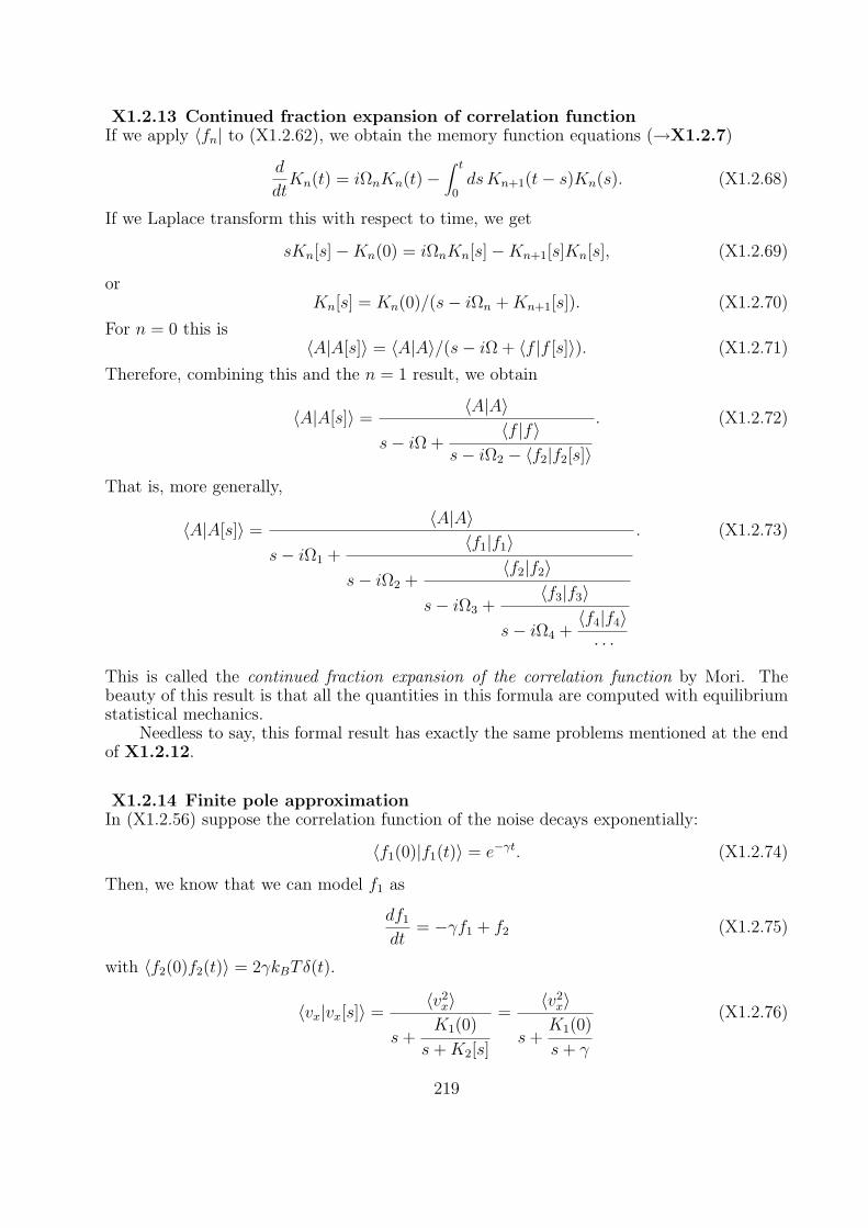
X1.2.13 Continued fraction expansion of correlation functionIf we apply 〈fn| to (X1.2.62), we obtain the memory function equations (→X1.2.7)

d

dtKn(t) = iΩnKn(t)−

∫ t

0dsKn+1(t− s)Kn(s). (X1.2.68)

If we Laplace transform this with respect to time, we get

sKn[s]−Kn(0) = iΩnKn[s]−Kn+1[s]Kn[s], (X1.2.69)

orKn[s] = Kn(0)/(s− iΩn +Kn+1[s]). (X1.2.70)

For n = 0 this is〈A|A[s]〉 = 〈A|A〉/(s− iΩ + 〈f |f [s]〉). (X1.2.71)

Therefore, combining this and the n = 1 result, we obtain

〈A|A[s]〉 =〈A|A〉

s− iΩ +〈f |f〉

s− iΩ2 − 〈f2|f2[s]〉

. (X1.2.72)

That is, more generally,

〈A|A[s]〉 =〈A|A〉

s− iΩ1 +〈f1|f1〉

s− iΩ2 +〈f2|f2〉

s− iΩ3 +〈f3|f3〉

s− iΩ4 +〈f4|f4〉· · ·

. (X1.2.73)

This is called the continued fraction expansion of the correlation function by Mori. Thebeauty of this result is that all the quantities in this formula are computed with equilibriumstatistical mechanics.

Needless to say, this formal result has exactly the same problems mentioned at the endof X1.2.12.

X1.2.14 Finite pole approximationIn (X1.2.56) suppose the correlation function of the noise decays exponentially:

〈f1(0)|f1(t)〉 = e−γt. (X1.2.74)

Then, we know that we can model f1 as

df1

dt= −γf1 + f2 (X1.2.75)

with 〈f2(0)f2(t)〉 = 2γkBTδ(t).

〈vx|vx[s]〉 =〈v2x〉

s+K1(0)

s+K2[s]

=〈v2x〉

s+K1(0)

s+ γ

(X1.2.76)

219

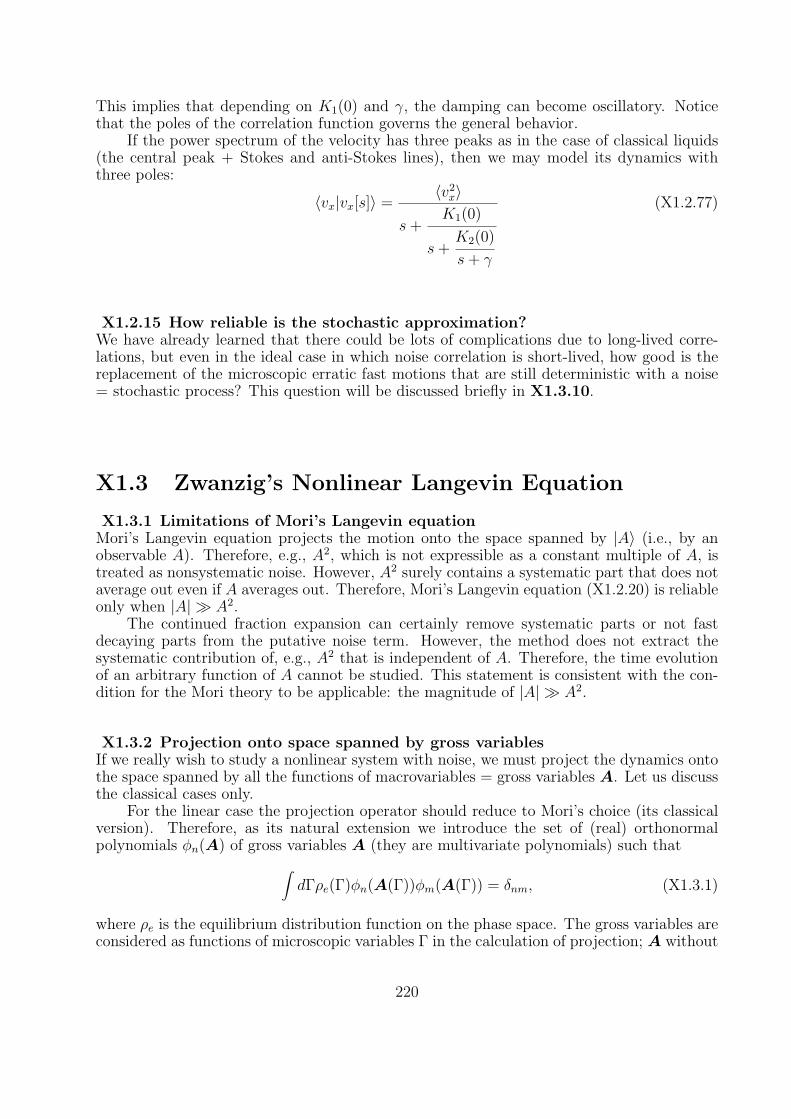
This implies that depending on K1(0) and γ, the damping can become oscillatory. Noticethat the poles of the correlation function governs the general behavior.

If the power spectrum of the velocity has three peaks as in the case of classical liquids(the central peak + Stokes and anti-Stokes lines), then we may model its dynamics withthree poles:

〈vx|vx[s]〉 =〈v2x〉

s+K1(0)

s+K2(0)

s+ γ

(X1.2.77)

X1.2.15 How reliable is the stochastic approximation?We have already learned that there could be lots of complications due to long-lived corre-lations, but even in the ideal case in which noise correlation is short-lived, how good is thereplacement of the microscopic erratic fast motions that are still deterministic with a noise= stochastic process? This question will be discussed briefly in X1.3.10.

X1.3 Zwanzig’s Nonlinear Langevin Equation

X1.3.1 Limitations of Mori’s Langevin equationMori’s Langevin equation projects the motion onto the space spanned by |A〉 (i.e., by anobservable A). Therefore, e.g., A2, which is not expressible as a constant multiple of A, istreated as nonsystematic noise. However, A2 surely contains a systematic part that does notaverage out even if A averages out. Therefore, Mori’s Langevin equation (X1.2.20) is reliableonly when |A| A2.

The continued fraction expansion can certainly remove systematic parts or not fastdecaying parts from the putative noise term. However, the method does not extract thesystematic contribution of, e.g., A2 that is independent of A. Therefore, the time evolutionof an arbitrary function of A cannot be studied. This statement is consistent with the con-dition for the Mori theory to be applicable: the magnitude of |A| A2.

X1.3.2 Projection onto space spanned by gross variablesIf we really wish to study a nonlinear system with noise, we must project the dynamics ontothe space spanned by all the functions of macrovariables = gross variables A. Let us discussthe classical cases only.

For the linear case the projection operator should reduce to Mori’s choice (its classicalversion). Therefore, as its natural extension we introduce the set of (real) orthonormalpolynomials φn(A) of gross variables A (they are multivariate polynomials) such that∫

dΓρe(Γ)φn(A(Γ))φm(A(Γ)) = δnm, (X1.3.1)

where ρe is the equilibrium distribution function on the phase space. The gross variables areconsidered as functions of microscopic variables Γ in the calculation of projection; A without

220

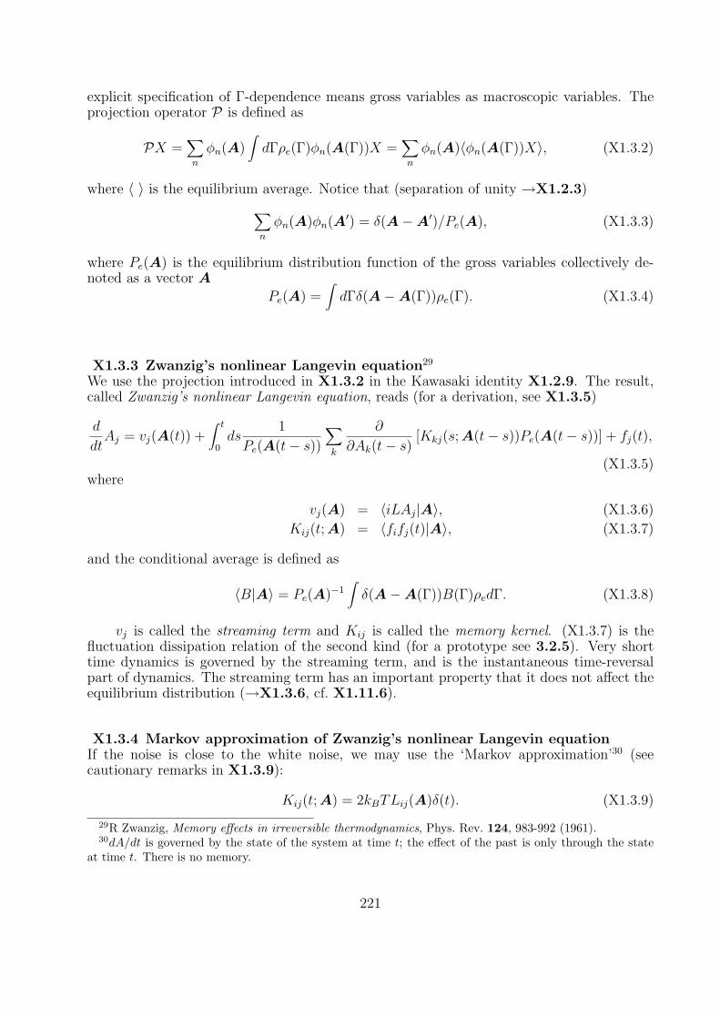
explicit specification of Γ-dependence means gross variables as macroscopic variables. Theprojection operator P is defined as

PX =∑n

φn(A)∫dΓρe(Γ)φn(A(Γ))X =

∑n

φn(A)〈φn(A(Γ))X〉, (X1.3.2)

where 〈 〉 is the equilibrium average. Notice that (separation of unity →X1.2.3)∑n

φn(A)φn(A′) = δ(A−A′)/Pe(A), (X1.3.3)

where Pe(A) is the equilibrium distribution function of the gross variables collectively de-noted as a vector A

Pe(A) =∫dΓδ(A−A(Γ))ρe(Γ). (X1.3.4)

X1.3.3 Zwanzig’s nonlinear Langevin equation29

We use the projection introduced in X1.3.2 in the Kawasaki identity X1.2.9. The result,called Zwanzig’s nonlinear Langevin equation, reads (for a derivation, see X1.3.5)

d

dtAj = vj(A(t)) +

∫ t

0ds

1

Pe(A(t− s))∑k

∂

∂Ak(t− s)[Kkj(s; A(t− s))Pe(A(t− s))] + fj(t),

(X1.3.5)where

vj(A) = 〈iLAj|A〉, (X1.3.6)

Kij(t; A) = 〈fifj(t)|A〉, (X1.3.7)

and the conditional average is defined as

〈B|A〉 = Pe(A)−1∫δ(A−A(Γ))B(Γ)ρedΓ. (X1.3.8)

vj is called the streaming term and Kij is called the memory kernel. (X1.3.7) is thefluctuation dissipation relation of the second kind (for a prototype see 3.2.5). Very shorttime dynamics is governed by the streaming term, and is the instantaneous time-reversalpart of dynamics. The streaming term has an important property that it does not affect theequilibrium distribution (→X1.3.6, cf. X1.11.6).

X1.3.4 Markov approximation of Zwanzig’s nonlinear Langevin equationIf the noise is close to the white noise, we may use the ‘Markov approximation’30 (seecautionary remarks in X1.3.9):

Kij(t; A) = 2kBTLij(A)δ(t). (X1.3.9)

29R Zwanzig, Memory effects in irreversible thermodynamics, Phys. Rev. 124, 983-992 (1961).30dA/dt is governed by the state of the system at time t; the effect of the past is only through the state

at time t. There is no memory.

221

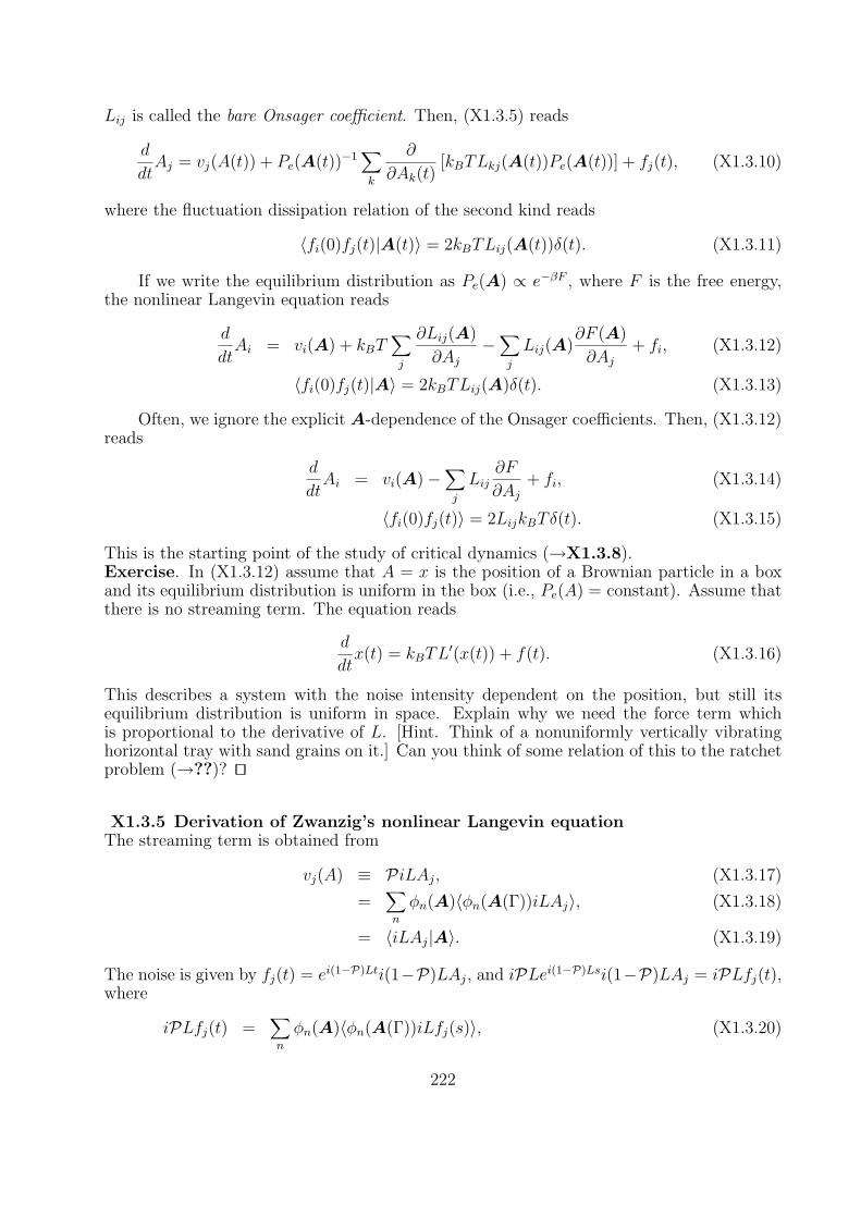
Lij is called the bare Onsager coefficient. Then, (X1.3.5) reads

d

dtAj = vj(A(t)) + Pe(A(t))−1

∑k

∂

∂Ak(t)[kBTLkj(A(t))Pe(A(t))] + fj(t), (X1.3.10)

where the fluctuation dissipation relation of the second kind reads

〈fi(0)fj(t)|A(t)〉 = 2kBTLij(A(t))δ(t). (X1.3.11)

If we write the equilibrium distribution as Pe(A) ∝ e−βF , where F is the free energy,the nonlinear Langevin equation reads

d

dtAi = vi(A) + kBT

∑j

∂Lij(A)

∂Aj−∑j

Lij(A)∂F (A)

∂Aj+ fi, (X1.3.12)

〈fi(0)fj(t)|A〉 = 2kBTLij(A)δ(t). (X1.3.13)

Often, we ignore the explicit A-dependence of the Onsager coefficients. Then, (X1.3.12)reads

d

dtAi = vi(A)−

∑j

Lij∂F

∂Aj+ fi, (X1.3.14)

〈fi(0)fj(t)〉 = 2LijkBTδ(t). (X1.3.15)

This is the starting point of the study of critical dynamics (→X1.3.8).Exercise. In (X1.3.12) assume that A = x is the position of a Brownian particle in a boxand its equilibrium distribution is uniform in the box (i.e., Pe(A) = constant). Assume thatthere is no streaming term. The equation reads

d

dtx(t) = kBTL

′(x(t)) + f(t). (X1.3.16)

This describes a system with the noise intensity dependent on the position, but still itsequilibrium distribution is uniform in space. Explain why we need the force term whichis proportional to the derivative of L. [Hint. Think of a nonuniformly vertically vibratinghorizontal tray with sand grains on it.] Can you think of some relation of this to the ratchetproblem (→??)? ut

X1.3.5 Derivation of Zwanzig’s nonlinear Langevin equationThe streaming term is obtained from

vj(A) ≡ PiLAj, (X1.3.17)

=∑n

φn(A)〈φn(A(Γ))iLAj〉, (X1.3.18)

= 〈iLAj|A〉. (X1.3.19)

The noise is given by fj(t) = ei(1−P)Lti(1−P)LAj, and iPLei(1−P)Lsi(1−P)LAj = iPLfj(t),where

iPLfj(t) =∑n

φn(A)〈φn(A(Γ))iLfj(s)〉, (X1.3.20)

222

= −∑n

φn(A)〈iLφn(A(Γ))fj(s)〉, (X1.3.21)

= −∑n

φn(A)∑k

〈iLAk(Γ) ∂φ

∂Ak(Γ)fj(s)〉, (X1.3.22)

= −∫dΓ∑k

iLAk(Γ) ∂

∂Ak(Γ)δ(A−A(Γ))Pe(A)−1fj(s)ρe(Γ),

(X1.3.23)

= −∫dΓ∑k

iLAk(Γ)fj(s)∂

∂Ak(Γ)δ(A−A(Γ))ρe(Γ)/Pe(A),

(X1.3.24)

= Pe(A)−1∑k

∂

∂Ak

∫dΓiLAk(Γ)fj(s)δ(A−A(Γ))ρe(Γ),

(X1.3.25)

= Pe(A)−1∑k

∂

∂Ak〈fkfj(s)|A〉Pe(A). (X1.3.26)

Combining all of these results, we obtain (X1.3.5).

X1.3.6 Streaming term does not affect equilibriumThe streaming term (X1.3.6) may be calculated further as

vj(A) = Pe(A)−1∫dΓδ(A−A(Γ))[Aj(Γ), H]PBρe(Γ), (X1.3.27)

= kBTPe(A)−1∫dΓδ(A−A(Γ))[Aj(Γ), ρe(Γ)]PB, (X1.3.28)

= kBTPe(A)−1∫dΓδ(A−A(Γ))

∑k

[Aj(Γ), Ak(Γ)]PB∂

∂Ak(Γ)ρe(Γ),

(X1.3.29)

= kBTPe(A)−1∑k

∂

∂Ak(〈[Aj(Γ), Ak(Γ)]PBA〉Pe(A)) . (X1.3.30)

Here, the conditional average in the last line is defined in (X1.3.8). To go from line 3 to 4,we have used integration by parts.

This term should not affect the equilibrium distribution function given by e−βF . Thatis, (→X1.7.1 or ??) ∑

j

∂

∂Ajvj(A)Pe(A) = 0. (X1.3.31)

This is immediate from the antisymmetry of the Poisson bracket in (X1.3.30).

X1.3.7 Mode coupling termsIf we use the expression of the projection in terms of the orthonormal polynomials, we have

vj(A) =∑n

φn(A)∫dΓφn(A(Γ))[Aj(Γ), H]ρe(Γ), (X1.3.32)

223

= −∑n

φn(A)∫dΓ kBTφn(A(Γ))[Aj(Γ), ρe(Γ)]PB, (X1.3.33)

=∑n

φn(A)∫dΓ kBT [Aj(Γ), φn(A(Γ))]PBρe(Γ). (X1.3.34)

That is,

vj(A) = kBT∑n

〈[φn(A(Γ)), Aj(Γ)]PB〉eφn(A) ≡∑n

v(n)v φn(A), (X1.3.35)

where 〈 〉e is the equilibrium average. In many applications we truncate this expansion atn = 2. The n = 2 terms are called mode-coupling terms.

X1.3.8 Mode-coupling equation for critical dynamicsIf we wish to study nonlinear dynamics of fluctuations, Pe is given by the thermodynamictheory of fluctuation (→2.8.5) as

Pe(A) ∝ exp(−∑j

A2j/2χj), (X1.3.36)

where χj is the susceptibility (→2.8.1). Since this is Gaussian, the multidimensional Her-mite polynomials are the most suitable orthonormal polynomials to construct projections(→X1.3.2):

φ(1)i = Ai/

√χi, (X1.3.37)

φ(2)ij = (AiAj − 〈AiAj〉e)/

√χiχj. (X1.3.38)

Here, 〈 〉e is the equilibrium average. From this it is easy to compute v(1)j and v

(2)j . Thus, we

obtain

vj(A) =∑k

iωjkAk +i

2

∑kl

Vjkl[AkAl − 〈AkAl〉e] (X1.3.39)

with

ωjk = −ikBT 〈[Aj, Ak]〉e/χk, (X1.3.40)

Vjkl = −ikBT 〈[Aj, AkAl]〉e/χkχl. (X1.3.41)

(X1.3.31) impliesωjk/χj = ωkj/χk (X1.3.42)

andVjkl/χj + Vklj/χk + Vljk/χl = 0. (X1.3.43)

The Langevin equation

dAjdt

=∑k

iωjkAk +i

2

∑kl

Vjkl[AkAl − 〈AkAl〉e]−∑k

LjkAkχk

+ fj (X1.3.44)

with 〈fifj(t)〉 = 2kBTLijδ(t) is the starting point of the mode coupling theory for criticaldynamics.31

31K. Kawasaki, Ann. Phys. 61, 1 (1970). The author told me that if he had known beforehand that thispaper was to be quoted so often, he should have written a better paper, but still this is a readable paper.

224

X1.3.9 Warning about white noise approximationIt has repeatedly been stressed that the essence of Brownian motion is that there are twodisparate time scales, macroscopic tM and mesoscopic τ 32 such that τ/tM 1 (e.g., X1.1.2).Also we have discussed that τ/tM → 0 is the limit to idealize this situation mathematically.However, we already know that in this limit the noise loses its continuity as a function of time(→3.7.6), so in (X1.3.12) A changes very rapidly, and deciding clearly whether a certainchange in A(t) (A at time t) is ‘before the delta function peak in (X1.3.13), after it, or witha more delicate relation to it’ becomes an important issue.

For physicists, the most sensible attitude is the following: Nothing is discontinuousdynamically: the fundamental equation of motion is a differential equation, so the coordi-nates q and p are at least once differentiable. Therefore, the idealization τ/tM → 0 mustbe performed after solving the differential equations (or after finishing all the integrations).Even quantum mechanically the basic equation of motion is a differential equation, so allthe natural changes of expectation values must be smooth.

However, it is also true that if we take this idealization limit and can assume that therapid increment of the noise term is always statistically independent of the A at the moment(this is equivalent to assuming the noise increment is independent; ‘after the delta functionpeak in (X1.3.13),’ so to speak), many calculations become simple.

In this idealization, the result of the calculation must agree with the physicists’ way ofcalculation: the idealization limit is taken after everything is over. To this end, we mustinvent a different calculus (Ito calculus) as already explained briefly in 3.4.4). This is thetopic of Section X1.5.

X1.3.10 Reliability of nonlinear reduction: Khas’minskii’s theoremConsider the following equation with two time scales

x(t) = f(x(t), ξ(t/ε)), (X1.3.45)

where f is a function, and ξ is a fast motion that does not depend on x. The reader mayimagine this is an external noise. Let the following limit exist:

limT→∞

1

T

∫ T

0dtf(u, ξ(t/ε)) = F (u), (X1.3.46)

where the time average is for fixed u. Modulo technical assumptions, Khas’minskii33 demon-strated the following:Up to the time scale of 1/ε2 xε(t) defined by the following set of equations (→X1.5.7 for aprecise definition) with the same initial condition as x(t) deviates at most of order ε fromx(t):

dxε(t) = F (xε(t)) +√εdη(t), (X1.3.47)

dη(t) = F ′(xε(t))η(t)dt+√D(xε(t))dB(t), (X1.3.48)

where B is the Wiener process (→X1.4.4), and

D(x) = limT→∞

1

T

∫ T

0dt∫ T

0ds (f(x, ξ(t/ε))− F (x))(f(x, ξ(s/ε))− F (x)). (X1.3.49)

32Often it is called the microscopic timescale.33R. Z. Khas’minskii, “A limit theorem for the solutions of differential equations with random right-hand

sides,” Theor. Prob. Appl. 11, 390-406 (1966).

225

That is, the effect of a rapidly changing perturbation may be mimicked by a systemwith a noise that is an Ornstein-Uhlenbeck process (→X1.8.9). The reader would say thisis not quite the assertion we wish to have, because in our case ξ depends on x(t).

In this case we wish to have an assertion like the following:Consider

x(t) = f(x(t), y(t)), y(t) =1

εg(x(t), y(t)). (X1.3.50)

In the ε → 0 limit, y is the fast variable. If the second member of the equation for each xdescribes a sufficiently chaotic dynamics,34 (X1.3.47) holds with F being defined as

F (x) = limT→∞

1

T

∫ T

0f(x, y(t))dt (X1.3.51)

and with the noise governed by (X1.3.48) with an appropriate replacement of D that caneasily be guessed. This type of theorems are now being proved by Kifer.35

Notice that these theorems are up to the time scale of 1/ε2. Beyond this scale we donot have any control. Hopefully, with the whole dynamics being sufficiently ergodic at leaston the average the solution to the reduced equation mimics the original system.

X1.4 Idealization of Brownian Motion: Wiener Pro-

cess

X1.4.1 Idealization of Brownian motionNow, we wish to idealize the Brownian motion, taking the time scale ratio τ/tM → 0 (fastnoise limit), where tM is the macroscopic time scale (the time scale of our observation; thismay perhaps be 1µs) and τ the mesoscopic time scale (this may be 10ps,36 so the ratio is10−5).

The simplest model of the Brownian motion in 1-space is

dx

dt= w(t), (X1.4.1)

where x is the position vector of the center of mass of a Brownian particle, and w describesthe effect of random noise; this equation describes an overdamped Brownian particle bom-barded by molecular collisions in a uniform space (ignoring the hydrodynamic effect).

Its idealization in the fast noise limit is, intuitively at least, to interpret w as a whitenoise. However, if we carefully think over the problem, we realize that ‘white noise’ has notbeen defined; we assert 〈w(t)w(s)〉 ∝ δ(t − s) (→3.2.4), so the equal-time correlation isunthinkable. This implies that w(t) is not a stochastic process in the usual sense = a mapfrom a probability space to a set of functions of time (→1.4.2).

34A precise characterization of this requirement is, for example, that for each x, the second member hasa unique SRB measure.

35Cf. Y. Kifer, “Averaging and climate models” in Progress in Probability, vol. 49 (P. Imkeller editor,Birkhauser, Basel, 2000).

36The oscillation of the CH bond stretching is of the order of 1fs = 1 ×10−15s.

226

X1.4.2 Heuristic construction of white noiseLet us try to construct a white noise w(t, ω). Here, the stochastic parameter ω is explicitlywritten. What we wish to require are:(i) ‘Whiteness’: all the frequency components have the same amplitudes.37

(ii) ‘Randomness’: all the frequency components are statistically independent.Let us make such a noise on the time span [0, 1].

If w(t, ω) is expanded in a Fourier series

w(t, ω) =∞∑

k=−∞ak(ω)ei2πkt, (X1.4.2)

(i) and (ii) imply that ak(ω)∞k=−∞ must be modeled as a set of iid (identically and inde-pendently distributed, cf. ??) stochastic variables. We choose they are Gaussian variables38

〈a†k(ω)aj(ω)〉 = δkj, 〈ak(ω)〉 = 0. (X1.4.3)

w(t, ω) is real, so a†−k = ak must be demanded.39

The convergence of the sum in (X1.4.2) is a non-trivial question, so we proceed intu-itively: the average must vanish

〈w(t, ω)〉 = 0. (X1.4.4)

The time correlation function reads40

〈w(s, ω)w(t, ω)〉 =∞∑

k=−∞e2πk(t−s) = δ(t− s). (X1.4.5)

X1.4.3 Construction of idealized Brownian motion = Wiener processLet us formally solve (X1.4.1) with the initial condition x(0, ω) = 0:41

x(t, ω) =∫ t

0w(s, ω)ds =

∞∑k=−∞

ak(ω)

2πik(ei2πkt − 1). (X1.4.6)

Here, the adverb ‘formally’ means that the summation and any operation are treated ascommutative.42 We see, then

〈x(t, ω)〉 = 0. (X1.4.7)

37This implies that all the harmonic modes have the same energy, so the total energy of a white noisediverges; that is why white noise is unthinkable as an ordinary stochastic process.

38If the simultaneous distribution of any finite subset of ak(ω)∞k=−∞ is Gaussian, we say the originalinfinite set is Gaussian-distributed.

39Then, how can we claim that ai(ω)∞k=−∞ is iid? In this case the interpretation is that the real and theimaginary parts of ak∞k=0 are iid stochastic variables (note that 〈ak(ω)2〉 = 0; what should 〈(Re ak(ω))2〉be?).

40Recall the Poisson summation formula.41For t = 1 x(1, ω) = a0(ω).42The reader who is familiar with the theory of Fourier series may suggest that we should use the Cesaro

sum, following the idea of Fejer. A similar idea indeed works (a theorem by Paley and Wiener; see Ito-McKean p21-2).

227

The correlation function reads

〈x(s, ω)x(t, ω)〉 = min(t, s). (X1.4.8)

We have constructed x with the aid of linear operations (summation and integration), so wemay intuitively expect that it is a Gaussian stochastic process.

The constructed process is in conformity with our intuitive picture of diffusing particles(cf. 3.1.8):

〈[x(t, ω)− x(s, ω)]2〉 = |t− s|. (X1.4.9)

That is, the displacement during time t behaves as√t.

A Gaussian process43 x(t, ω) satisfying (X1.4.7) and (X1.4.8) is called the Wiener pro-cess.

From the mathematician’s point of view that such a Gaussian process is indeed well-defined is a major triumph. Our construction can be fully justified with the aid of a stochas-tic process in the distribution sense, but a more traditional approach is outlined below inX1.4.5.

X1.4.4 Wiener process: definitionThrough our heuristic construction of the dynamics of a particle driven by a white noise,we have clearly grasped what sort of stochastic process we should study mathematically.Although we have only studied the process on [0, 1], it should not be hard to extend this forall nonnegative time.

An official definition of the Wiener process (mathematicians often call this Brownianmotion) is:Definition: Wiener processThe Wiener process B is a stochastic process B(t, ω) : t ∈ [0,∞), ω ∈ Ω44 satisfying thefollowing conditions:(A) B(0, ω) = 0 with probability one.(B) for any positive integer n and 0 < t1 < · · · < tn the increments

B(t1), B(t2)−B(t1), · · · , B(tn)−B(tn−1) (X1.4.10)

are independently and normally distributed (i.e., Gaussian) with mean 0 and variance

t1, t2 − t1, · · · , tn − tn−1 (X1.4.11)

(C) B(t, ω) is continuous with probability 1.The conditions are not minimal: the reader can say that if a process satisfies (A) and

(B), then it is possible to construct a model with (C). Or, for physicists it should be appeal-ing that (A) + (C) + independent increments (the first part of (B)) implies the second partof (B) (that is, if we assume continuity and independent increments, then the central limittheorem (→1.7.1) forces us to swallow Gaussianness).45

Giving a definition is one thing, and demonstrating the existence is another; we could

43A stochastic process whose any finite dimensional marginal distribution is Gaussian is called a Gaussianprocess.

44on a probability space Ω,F , P.45See Durrett, p334.

228

define a unicorn! The existence was first shown by Wiener in 1923.46 An argument probablymost appealing to physicists (except for the renormalization group approach →X1.4.10) isoutlined in X1.4.5.47

X1.4.5 Outline of mathematical construction of Wiener process.This is essentially a rigorization of our intuitive construction: X1.4.3 suggests

Bn(t, ω) =n∑j=0

ηj(ω)Φj(t) (X1.4.12)

converges to B in the n→∞ limit, where ηi are iid stochastic variables obeying N(0, 1) and

Φj(t) =∫ t

0ds φj(t) (X1.4.13)

with φj(t) being a complete orthonormal function set on [0,∞). We can show that Bn(t, ω)almost surely converges to B(t, ω)48 with the aid of Levy’s three series convergence theorem:Theorem [Levy] Let Xn be independently distributed. Then, for the sum

∑Xn, its con-

vergence in probability, almost sure convergence, and convergence in law are equivalent.49 utTherefore, we have only to show the convergence in the mean (that implies convergence inprobability) of Bn, but this is a mere exercise.Exercise. Demonstrate that E[Bn(t, ω)2] ≤ t. ut

X1.4.6 Important properties of Wiener processWe are interested in the properties of sample paths: the properties of B(t, ω) for a fixed ω.

By construction, it is almost surely50 continuous. However,Non-differentiability: B(t, ω) is nowhere differentiable with probability one.51

This is exactly what Perrin asserted (→3.1.5, 3.4.1).Stationarity (or translational symmetry): for any positive number a B(t+a, ω)−B(a, ω), t ≥0 is again the Wiener process.This is easy to check. This means that if we can show that some statement holds withprobability one at one time, we may claim the same statement at any other time.Scaling invariance (or self-similarity): for any positive number λ λ−1B(λ2t, ω), t ≥ 0 isagain the Wiener process.This is also easy to check.Conformal invariance: tB(1/t, ω), t ≥ 0 is again the Wiener process.This is easy to check. The very short time behavior magnified appropriately looks like a longtime behavior.

46This year: France occupied the Ruhr, Munchen Putsch; Hubble discovered extragalactic spiral galaxies;the first issue of Time magazine.

47Perhaps the easiest proof may be found in D. Freedman, Brownian Motion and Diffusion (Springer,1983). As always, a smart proof is in Durrett, p335.

48It is known that the convergence is actually uniform in t.49Convergence in law may be understood as the convergence of characteristic functions.50This is a statement equivalent to “with probability 1.”51Not Lipschitz at any point. However, it is Holder continuous with exponent less than 1/2 with probability

one. The Hausdorff dimension of a sample path is 2 with probability 1.

229

X1.4.7 Increments are roughly of order√t

The translational and scaling invariance (→X1.4.6) imply that statistically B(t + δt, ω) −B(t, ω) and

√δtB(1, ω) are indistinguishable. Therefore, short time increment behaves like√

t. This is of course what Einstein pointed out (→3.1.5).There are two related statements:

2n∑m=1

[B(mt

2n

)−B

((m− 1)t

2n

)]2

→ t (X1.4.14)

with probability one as n→∞. However,

lim supt→0

B(t, ω)/√t =∞. (X1.4.15)

That is, the amplitude ‘overshoots’√t.

A more precise statement about this overshoot is the law of iterated logarithm:

sup |B(t+ h)−B(t)| ∼√

2h log log(1/h) (X1.4.16)

in the h→ 0 limit. Or, using the conformal invariance (→X1.4.6), almost surely

lim supt→∞

B(t, ω)/√

2t log log t = 1. (X1.4.17)

This is Khintchine’s celebrated law of iterated logarithm.52

X1.4.8 Markov property of Wiener processBy definition (→X1.4.4) the Wiener process has independent increments, so the conditionalprobability of B(t, ω) under the condition that we know ‘everything’ about it up to time smust be identical to the conditional probability under the condition that we know onlyB(s, ω). This is mathematically expressed as

P (B(t, ω)|Fs) = P (B(t, ω)|B(s, ω)), (X1.4.18)

where Fs is the set of all the events up to time s.53

X1.4.9 n-dimensional Wiener processPrepare n statistically independent Wiener processesB1(t, ω), · · · , Bn(t, ω). B(t, ω) = (B1(t, ω), · · · , Bn(t, ω))T

is called the n-dimensional Wiener process.

〈B(t, ω) ·B(t, ω)〉 = nt. (X1.4.19)

52This is a refinement of the central limit theorem. For a proof see Durrett p392.53Here, ‘all’ implies, as usual, all the probabilistically meaningful events. See 1.A.20. The Markov process

will be discussed later in Chapter 9.

230

X1.4.10 From random walk to Wiener process: ideaConsider an isotropic random walk (→3.1.8) on a line. At time k (k = 0, 1, 2, 3, · · ·) awalker at a lattice point moves to its left or right nearest neighbor lattice point with equalprobability 1/2. Let x(n) be the walker’s position at time n, and ak be the k-th step (i.e.,the step between time k − 1 and k). Then,

x(n) =n∑k=1

ak. (X1.4.20)

This exactly has the form of the empirical sum Sn in the central limit theorem (→1.7.1).What does the walk look like if seen from distance, when the duration of the random

walk is sufficiently long (that is, n 1)? To answer this question, we mimic the observationby an observer with a limited eyesight. To mimic a limited resolution, we define a coarse-grained ‘block step’ Sn by connecting n consecutive steps. To mimic an observation fromdistance we scale it with

√n, because the span of the random walk is of order

√n (→3.1.8).

Finally, we take the n → ∞ limit. The limit should be what we wish to have. This idea isfollowed in X1.4.11.

X1.4.11 Construction of coarse-grained and scaled random walkWe introduce a piecewise linear continuous time version of a discrete time random walkthrough linear interpolation:

S(nt) = a1 + · · ·+ a[nt] + (nt− [nt])a[nt]+1, (X1.4.21)

where the i-th step ai is ±1, and t ∈ [0, 1]. These steps are identically and independentlydistributed. Now, we scale this to define

Bn(t) =1√nS(nt). (X1.4.22)

We may say this is a renormalized random walk.Thanks to the central limit theorem (→1.7.1), for any fixed t, it is easy to show that

the distribution of Bn(t) converges to N(0, t). To check this we have only to compute thevariance. Obviously,

E(S([nt])2) = [nt]. (X1.4.23)

Due to the construction, for any finite time points t1, t2, · · · , tN ∈ [0, 1], the simultaneousdistribution of Bn(t1), · · · , Bn(tN) converges weakly to that of B(t1), · · · , B(tN), whereB is the Wiener process (→X1.4.4). This is almost trivial. Thus, we expect Bn convergesto B in a certain sense.

X1.4.12 Donsker’s invariance principle (continuation of X1.4.11)Theorem [Donsker (1951)] Bn converges to the Wiener process B in distribution (i.e., theweak convergence of the corresponding measure). utThis is called Donsker’s invariance principle. Here, ‘invariance’ implies that “many differentrandom walks converge invariably to the Wiener process.” The procedure in X1.4.11 is arenormalization-group procedure, so a better name may be ‘Donsker’s universality principle’and for physicists Donsker’s theorem should be remembered as:

231

Theorem [Donsker restated] The fixed point of the renormalization transformation RBn =B2n (defined according to X1.4.11) is the Wiener Process (i.e., RB = B). ut

In X1.4.11 the convergence of the any finite-dimensional marginal distribution is men-tioned, but this does not necessarily imply the convergence in the function space, becausesimple counter examples can be found.54 Therefore, the nontrivial part is to show the con-vergence in distribution of Bn(t) to B(t).

X1.4.13 Idea for demonstrating Donsker’s theorem.We need ‘stochastic compactness’, so to speak, to be able to choose a convergent sequence. In essence weneed a probabilistic version of the Arzela-Azcoli theorem called Prohorov’s theorem:Theorem [Prohorov] Let Π be a set of probability measures on a probability space. The set is relativelycompact iff it is tight. utHere, the technical terms are:Relative compactness: every sequence has a weakly convergent subsequence.Tightness: For any ε > 0 there is a compact set K such that for any element µ in Π µ(K) > 1− ε.

The tightness of Π is characterized as follows:(i) Probabilistic boundedness: For any η there is a such that µn(|x(0)| ≥ a) < η.(ii) Probabilistic equicontinuity: For any ε and η, there is δ ∈ (0, 1) such that µn(sup|s−t|<δ |x(s)− x(t)| ≥ε) ≤ η.This is, so to speak, ‘a probabilistic version of the Arzela-Azcoli theorem.’

Note the following theorem:Theorem A necessary and sufficient condition for Pn to converge to P weakly is that each subsequencePni contains a further subsequence converging weakly to P . utNecessity is obvious. The other direction is also easy; if not, there must be a subsequence not converging toP , and this subsequence cannot have a further subsequence with the required property.

Therefore, if we accept Prohorov, we haveTheorem Let Pn and P be probability measures.55 Suppose all the finite dimensional marginal distributionsof Pn converge to those of P , and Pn is tight, then Pn converges to P weakly. ut

Since we know the existence of B, we have only to check the tightness of Bn.

X1.4.14 Global properties of random walks survive RGIf we compare the starting point (lattice random walk) and the final product (the Wienerprocess) of the ‘renormalization-group (RG) construction’ in X1.4.11, we clearly understandwhat RG does: it washes away details, and only the features we can observe from distancesurvive.

Look at the following table in which d is the spatial dimensionality.

Lattice Random Walk Wiener Processd = 2 recurrent d = 2 recurrentd > 2 transient d > 2 transient〈R2〉 ∝ N 〈R2〉 ∝ t∃ double points in any d ∃ double points only for d ≤ 3For all d the numbers of n(≥ 3)-tuple ∃ n(≥ 3)-tuplepoints are proportional to N points only in d = 2.†

54Recall that the joint set of countably many finite sets is a countable set, so most points in R are alwaysexcluded.

55on C([0, 1]) with the uniform topology and with the usual construction of the Borel family.

232

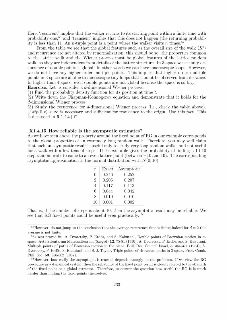
Here, ‘recurrent’ implies that the walker returns to its starting point within a finite time withprobability one,56 and ‘transient’ implies that this does not happen (the returning probabil-ity is less than 1). An n-tuple point is a point where the walker visits n times.57

From the table we see that the global features such as the overall size of the walk 〈R2〉and recurrence are not altered by renormalization; this should be so: the properties commonto the lattice walk and the Wiener process must be global features of the lattice randomwalk, so they are independent from details of the lattice structure. In 3-space we see only oc-currence of double points is global. In other words we can have macroscopic loops. However,we do not have any higher order multiple points. This implies that higher order multiplepoints in 3-space are all due to microscopic tiny loops that cannot be observed from distance.In higher than 4-space, even double points are not global because the space is so big.Exercise. Let us consider a d-dimensional Wiener process.(1) Find the probability density function for its position at time t.(2) Write down the Chapman-Kolmogorov equation and demonstrate that it holds for thed-dimensional Wiener process.(3) Study the recurrence for d-dimensional Wiener process (i.e., check the table above).[∫dtp(0, t) < ∞ is necessary and sufficient for transience to the origin. Use this fact. This

is discussed in 6.1.14.] ut

X1.4.15 How reliable is the asymptotic estimates?As we have seen above the property around the fixed point of RG in our example correspondsto the global properties of an extremely long random walk. Therefore, you may well claimthat such an asymptotic result is useful only to study very long random walks, and not usefulfor a walk with a few tens of steps. The next table gives the probability of finding a 1d 10step random walk to come to an even lattice point (between −10 and 10). The correspondingasymptotic approximation is the normal distribution with N(0, 10)

r Exact Asymptotic0 0.246 0.2522 0.205 0.2074 0.117 0.1136 0.044 0.0428 0.010 0.01010 0.001 0.002

That is, if the number of steps is about 10, then the asymptotic result may be reliable. Wesee that RG fixed points could be useful even practically. 58

56However, do not jump to the conclusion that the average recurrence time is finite; indeed for d = 2 thisaverage is not finite.

57∗ was proved in: A. Dvoretsky, P. Erdos, and S. Kakutani, Double points of Brownian motion in n-space, Acta Scientarum Matematicarum (Szeged) 12, 75-81 (1950); A. Dvoretsky, P. Erdos, and S. Kakutani,Multiple points of paths of Brownian motion in the plane, Bull. Res. Council Israel, 3, 364-371 (1954); A.Dvoretsky, P. Erdos, S. Kakutani, and S. J. Taylor, Triple points of Brownian paths in 3-space, Proc. Camb.Phil. Soc. 53, 856-862 (1957).

58However, how easily the asymptopia is reached depends strongly on the problems. If we view the RGprocedure as a dynamical system, then the reliability of the fixed point result is closely related to the strengthof the fixed point as a global attractor. Therefore, to answer the question how useful the RG is is muchharder than finding the fixed points themselves.

233

X1.5 Stochastic Calculus

This section is an informal introduction to stochastic calculus now famous thanks to theBlack-Scholes equation. Motivations of needed ideas are explained rather slowly, so thosewho are impatient can read the summary X1.5.1 and the quoted final results.

X1.5.1 Stochastic calculus: practical summary of this sectionA nonlinear Langevin equation

dx

dt= a(x, t) + σ(x, t)w, (X1.5.1)

where w is the normalized white noise is mathematically the stochastic differential equation

dx = a(x, t) + σ(x, t)dB, (X1.5.2)

which is defined as a shorthand notation of the following integral equation (→X1.5.7):

x(t)− x(0) =∫ t

0ds a(x(s), s) +

∫ t

0σ(x(s), s)dB(s). (X1.5.3)

Here, the last term is defined as an Ito integral X1.5.6.The difficulty is due to dB ∼

√dt (→X1.4.7). To use the above machinery first

we must properly interpret the Langevin equation (→X1.5.8, X1.5.13). With stochasticcalculus, we can have the most straightforward derivation of the Fokker-Planck equation(→X1.5.14). Stochastic calculus is a prerequisite for easy access to the Feynman-Kac for-mulas (→X1.10.1) and path integrals (→X1.10.2).

X1.5.2 How to rationalize idealized Langevin equationWe have rationalized the Wiener process (→X1.4.4) that is supposedly a solution to (X1.4.1),so the white noise in this equation is the ‘derivative’ of the Wiener process. However, wehave seen that it is not differentiable anywhere with probability one (→X1.4.6). Therefore,for example,

dx

dt= −ηx+ ‘

dB

dt’ (X1.5.4)

does not make sense yet. Its formal solution can be written as

x(t) = e−ηtx(0) +B(t)− η∫ t

0dse−η(t−s)B(s)ds, (X1.5.5)

if we use the following formal integration by parts:∫ t

0f(s)dB(s) = f(t)B(t)−

∫ t

0f ′(s)B(s)ds. (X1.5.6)

Its right-hand-side is mathematically well-defined, because B is continuous, so we wish todefine the Riemann-Stieltjes integral (→X1.5.4) on the left-hand-side in terms of the right-hand side.

234

The solution (X1.5.5) agrees with the result obtained by the following ‘non-ideal’ calcu-

lation. Assuming that w = dB/dt with B being a noise that is differentiable (its correlationfunction is an ordinary continuous function at worst). Our familiar ordinary calculus can beused freely, and we obtain

x(t) = e−ηtx(0) + B(t)− η∫ t

0dse−η(t−s)B(s)ds. (X1.5.7)

Now, we take the white noise limit. The result is consistent with (X1.5.5).Thus, when the noise amplitude does not depend on x (may depend on t), we interpret

dx

dt= a(x) + σ(t)‘

dB

dt’ (X1.5.8)

asdx(t) = a(x(t))dt+ σ(t)dB(t), (X1.5.9)

which is interpreted as a short-hand notation of the following integral equation

x(t)− x(0) =∫ t

0ds a(x(s)) +

∫ t

0σ(s)dB(s). (X1.5.10)

The last term is interpreted as (X1.5.6).That is, we define (X1.5.9) as a short hand notation of the integral equation (X1.5.10).

X1.5.3 How to rationalize nonlinear Langevin equationWe are tempted to interpret (define) the general nonlinear Langevin equation, e.g., Zwanzig’snonlinear Langevin equation (→X1.3.3), with the normalized white noise w

dx

dt= a(x, t) + σ(x, t)w (X1.5.11)

as the following integral equation:

x(t)− x(0) =∫ t

0ds a(x(s), s) +

∫ t

0σ(x(s), s)dB(s), (X1.5.12)

interpreting the last integral as a Riemann-Stieltjes integral (→X1.5.4).As we will see later (→X1.5.7), this idea works eventually, but there are obstacles.

The difficulty is essentially the one we have already pointed out: it is not clear whether thenoise-increment could affect x(s) or not. If dB(t) = B(t + dt) − B(t) were of order dt, wedid not have to worry about such details at all; the difference is at worst dt2. However, inour case this quantity is roughly of order

√dt (→X1.4.7), so its square cannot be ignored.

In short, rapid change of noise causes a headache; if a system is sufficiently nonlinear, thenoise effect does not simply average out.

Therefore, if we wish to invent a method of calculation that allows taking the whitenoise limit before any calculation, we must scrutinize the last term in (X1.5.12).

X1.5.4 Riemann-Stieltjes integrationThe Riemann-Stieltjes integral is defined as the following limit∫ b

af(x)dg(x) = lim

‖∆‖→0

∑∆

f(xi)[g(bi)− g(ai)], (X1.5.13)

235

where xi ∈ ∆i ≡ [ai, bi] and ‖∆‖ = maxbi−ai.59 It is known that a necessary and sufficientcondition60 for this limit to exist is that g is of bounded-variation:

v(g) ≡ sup∆

∑i

|g(bi)− g(ai)| <∞. (X1.5.14)

Here, v(g) is called the total variation of g on [a, b]. Here, sup is taken over all possible finitepartition (chopping up) of [a, b].

If g is not of bounded variation, the sum in (X1.5.13) depends on the position of thesampling points xi on each ∆i.

If the function g is Lipschitz continuous,61 this is finite. However, mere continuity doesnot guarantee the boundedness of its total variation v(g).

What happens in the case of the Wiener process B (→X1.4.4)? We can easily guessthat B(t, ω) on [0, 1] is not of bounded variation: Let us chop up [0, 1] into small intervals

of width ∆t. Then, we have 1/∆t intervals on each of which B varies of order√

∆t, so

v(B) ∼ 1/√

∆t.Therefore, the integral

∫ t0 σ(x(s))dB(s) must be defined more carefully. Indeed, as we

seen in X1.5.5 the integral depends on the sampling method of the representative values.

X1.5.5 Backward and forward integralsLet us take a smooth function f and consider the following sums:

SF (n) =n∑k=1

f

(B

((k − 1)t

n

))[B

(kt

n

)−B

((k − 1)t

n

)], (X1.5.15)

SB(n) =n∑k=1

f

(B

(kt

n

))[B

(kt

n

)−B

((k − 1)t

n

)], (X1.5.16)

where B is the Wiener process (→X1.4.4). SF is called the forward sum, because the noiseincrement goes ahead of the sampling time; SB is called the backward sum.

It is easy to see that they give different values even if convergent: the expectation valueof SF vanishes because of the independence of the increment (→X1.4.4), but SB is generallynonzero. We can easily guess that the difference is

limn→∞

(SB(n)− SF (n)) =∫ t

0dsf ′(B(s)). (X1.5.17)

It is clear that if we can define the ‘stochastic integral’ by the limit of the forward sum,then calculation of expectation values should be easy. The integral defined in this forwardway is called Ito integral.

59Precisely speaking, if the limit exists for any choice of the partition sequence and the sampling pointsxi.

60See, for example, P. Protter, Stochastic Integration and Differential Equations (Springer, 1990) Section1.7.

61A function is Lipshitz continuous at x, if we can find a positive constant L such that

|f(x)− f(y)| < L|x− y|

for any y in the domain of f . For example, |x| is Lipshitz continuous everywhere, but√|x| is not so at

x = 0.

236

X1.5.6 Definition of Ito integralWe define the stochastic integral (Ito integral) as the limit of the regular forward Riemann-Stieltjes sum (for a motivation →X1.5.5):

∫ t

0f(s)dB(s) ≡ lim

n→∞

n∑k=1

f

(B

((k − 1)t

n

))[B

(kt

n

)−B

((k − 1)t

n

)]. (X1.5.18)

The convergence (that must be demonstrated for continuous functions f) is in the almostsure sense.

X1.5.7 Definition of stochastic differential equationWe interpret the nonlinear Langevin equation (X1.5.11) as a shorthand notation of (X1.5.12)with the last integral interpreted in Ito’s sense. That is:The differential relation (called a stochastic differential equation):

dx = a(x, t) + σ(x, t)dB (X1.5.19)

is defined as a shorthand notation of the following integral equation:

x(t)− x(0) =∫ t

0ds a(x(s), s) +

∫ t

0σ(x(s), s)dB(s), (X1.5.20)

where the last term is defined as an Ito integral X1.5.6.Notice that Zwanzig’s Langevin equation must, by derivation (→X1.3.5),62 be inter-

preted in Ito’s sense.

X1.5.8 Physical equations with noise vs stochastic differential equationsFor physicists physical noises are all of bounded variation (→X1.5.4), so Ito’s specificationis often unphysical. That is, the ideal white noise limit of the solution to the following‘physical’ Langevin equation

dx

dt= a(x, t) + σ(x, t)

dB

dt(X1.5.21)

and the solution to the stochastic differential equation

dx(t) = a(x, t)dt+ σ(x, t)dB(t) (X1.5.22)

generally do not agree.Since mathematically and even from the practical computational point of view, Ito’s

interpretation is far more superior than other interpretations, and since for physicists thisinterpretation is not necessarily natural, we should have a way to translate different inter-pretations (→X1.5.13; X1.5.9 is a preparation).Warning: However, if a stochastic differential equation is derived through projection, youmust scrutinize the derivation before deciding the interpretation. ut

62Notice that the noise f(t) is always computed with the condition A(t) and then evolving in time, so theincrement df is not affecting A(t).

237

X1.5.9 Ito’s lemma: heuristic considerationLet u be a function of t and the Wiener process B(t) (→X1.4.4). Taylor-expanding u, wehave

u(t+ ∆t, B(t+ ∆t))− u(t, B(t))

= ∆t∂u

∂t+ ∆B(t)

∂u

∂B+

1

2(∆t)2∂

2u

∂t2+ ∆t∆B

∂2u

∂t∂B+

1

2(∆B)2 ∂

2u

∂B2+ · · · ,

(X1.5.23)

where ∆B(t) = B(t + ∆t) − B(t). Among the formally second order terms, the dangerous

term is only the last term, because ∆B ∼√

∆t (→X1.4.7).Summing this from t = 0 to T , we can express u(T,B(T )) as an integral of the following

form

u(T,B(T ))− u(0, 0) =∫ T

0

∂u

∂tds+

∫ T

0

∂u

∂BdB(s) +

1

2

∫ T

0

∂2u

∂B2dt. (X1.5.24)

Here, the stochastic integral (the second term on the right hand side) is in Ito’s sense(→X1.5.6). That is, almost surely

du(t, B) =

(∂u

∂t+

1

2

∂2u

∂B2

)dt+

∂u

∂BdB. (X1.5.25)

To demonstrate (X1.5.24), the nontrivial part is to show that almost surely

∑ 1

2(∆B)2 ∂

2u

∂B2→ 1

2

∫ T

0

∂2u

∂B2dt. (X1.5.26)

The first step is to show this is true in the mean (in the L2-sense), and then we use the factthat we can choose a subsequence that almost surely converges.

X1.5.10 Ito’s lemma: general caseIf dx = adt+ σdB, it is easy to generalize (X1.5.25) as63

du(t, x) =

(∂u

∂t+σ2

2

∂2u

∂x2

)dt+

∂u

∂xdx. (X1.5.27)

This is called Ito’s lemma. An easy way to memorize it is

du =∂u

∂tdt+

∂u

∂xdx+

1

2

∂2u

∂x2dx2 (X1.5.28)

with the rule dB2 = dt (so dx2 = σ2dt; other cross terms are of higher order).Exercise.(1) Compute d sinB(t). Then, check that d〈sinB(t)〉 = −〈sinB〉dt/2.(2) Compute d sin(ωt+ εB(t)). Demonstrate that its average decays eventually to zero. (Wealready did this calculation!).(3) Compute d exp(B(t)− t/2), and then find the general solution to df = fdB(t) for f .(4) Suppose dx = −xdt+

√2xdB. Compute dx2. Then, study the time-dependence of 〈x2〉.64

ut63A fairly readable (but you must be patient when you read math books) proof can be found in Z. Brzezniak

and T. Zastawniak, Basic Stochastic Processes (Springer, 1998).64This is a very pathological example. Think how pathological it is. Is there any stationary distribution?

238

X1.5.11 Ito integral: examplesLet us first compute the forward sum SF (→X1.5.5) in the n → ∞ limit for an integrablefunction f . According to Ito’s lemma65 (→X1.5.10)

d[∫ x

0f(x′)dx′

]x=B(t)

= f(B(t))dB(t) +1

2f ′(B(t))dt. (X1.5.29)

Here, the integral on the left-hand side is an ordinary integral. Thus, we have obtained

limn→∞

SF (n) =∫ t

0f(B(s))dB(s) =

∫ B(t)

0f(x)dx− 1

2

∫ t

0dsf ′(B(s)). (X1.5.30)

Notice that the average must be zero. Therefore,⟨∫ B(t)

0f(x)dx

⟩=

1

2

∫ t

0ds〈f ′(B(s))〉. (X1.5.31)

More concrete examples follow:∫ t

0B(s)dB(s) =

1

2(B(t)2 − t). (X1.5.32)

Indeed, its average vanishes by definition of the Winer process: 〈B(t)2〉 = t.∫ t

0eBdB =

∫ B

0exdx− 1

2

∫ t

0eB(s)ds. (X1.5.33)

Since B(t) is Gaussian 〈eB〉 = e〈B2〉/2 = et/2, we can explicitly check that this is correct.

Exercise.(1) Compute

∫e3BdB and demonstrate that its expectation value vanishes.

(2) Let dp = −(ζ/m)pdt+√

2kBTζdB. Compute dp2, and then study the time dependenceof its average 〈p2〉.ut

X1.5.12 Wong-Zakai’s theorem: motivationFor physicists all the noises are of bounded variation (→X1.5.4), so

I =∫ t

0f(B(s))dB(s) =

∫ B(s)

0f(x)dx. (X1.5.34)

Therefore, taking the ideal white noise limit of this integral, we must have

I →∫ B(t)

0f(x)dx =

∫ t

0f(B(s))dB(s) +

1

2

∫ t

0f ′(B(s))ds. (X1.5.35)

This follows from the usual Ito’s lemma (→X1.5.10):

d∫ B(t)

0f(x)dx = f(B(t))dB(t) +

1

2f ′(B(t))dt, (X1.5.36)

65Warning: If the integral inside the square brackets is understood as Ito’s integral, by definition(→X1.5.7) d

∫f(x)dx = f(x)dx. No extra term appears. Here, it is an ordinary integral; after finish-

ing the integral we put B in the integral result (in the primitive function of f).

239

The short-hand notation for this integral relation is

f(B) dB = f(B)dB +1

2f ′(B)(dB)2, (X1.5.37)

where implies that we take the white noise limit after performing the integral, assumingthat the noise of B is of bounded variation (→X1.5.4).

More, generally, if dx = adt+ σdB, then the idealization limit should read

f(x) dB = f(x)dB +1

2f ′(x)dxdB = f(x)dB +

1

2f ′(x)σdt. (X1.5.38)

X1.5.13 Wong-Zakai’s theoremSuppose we write down a stochastic differential equation (Langevin equation) physically,assuming that the noise is of bounded variation (→X1.5.4) as (→X1.5.12 for )

dx = a(x, t)dt+ σ(x, t) dB. (X1.5.39)

Here, is used to denote clearly that the term is NOT interpreted in Ito’s sense, but in theusual calculus sense.66 If we wish to use the Ito calculus, we must rewrite this as (→(X1.5.38))

dx =

(a(x, t) +

1

2σ∂σ

∂x

)dt+ σ(x, t)dB. (X1.5.40)

That is, we must augment the extra term in (X1.5.38). The relation between (X1.5.39) and(X1.5.40) is called Wong-Zakai’s theorem.Exercise 1. Suppose a variable is described by the following stochastic differential equation(in the standard sense)

dx =√f(x)dB. (X1.5.41)

We know the average of x is time independent. That is, the noise cannot drive the particleon the average. Suppose we wish to model this with a physical noise. If we study

dx

dt=√f(x)w, (X1.5.42)

where w is a random noise (not quite white), then we see that x is time dependent on theaverage.(1) Find the equation for the average 〈x(t)〉.(2) Therefore, the reader realizes that to model (X1.5.41) she must add a systematic drive.Find a physical model that mimics (X1.5.41). [This is a trivial question if the reader hasanswered (1).] ut

X1.5.14 Derivation of Fokker-Planck equation: a smart wayLet dx = adt+σdB. We know the density distribution function of x at time t reads (→1.4.5)

P (y, t) = 〈δ(y − x(t))〉. (X1.5.43)

66Often we say in Stratonovich’s sense.

240

Let us derive the Fokker-Planck equation with the aid of Ito calculus (→X1.5.10):

dδ(y − x(t)) = − ∂

∂yδ(y − x(t))dx(t) +

1

2

∂2

∂y2δ(y − x(t))σ2(x(t), t)dt (X1.5.44)

= − ∂

∂yδ(y − x(t))[a(x(t), t)dt+ σ(x(t), t)dB(t)] +

1

2

∂2

∂y2δ(y − x(t))σ2(x(t), t)dt.

(X1.5.45)

Let us take the average over the stochastic parameter:

dP (y, t) = − ∂

∂ya(y, t)P (y, t)dt+

1

2

∂2

∂y2σ(y, t)2P (y, t)dt. (X1.5.46)

Thus, we have arrived at

∂

∂tP (y, t) = − ∂

∂ya(y, t)P (y, t) +

1

2

∂2

∂y2σ(y, t)2P (y, t). (X1.5.47)

This is the stochastic Liouville approach (→??) combined with the Ito’s lemma (→X1.5.10);perhaps this is the easiest derivation of the Fokker-Planck (or Smoluchowski) equation.

241

X1.6 Stochastic Energetics

This section is largely dependent on Ken Sekimoto’s lecture notes in 1999 for a graduatecourse at Kyoto University (but perhaps uses stochastic calculus more extensively).

X1.6.1 How good is Langevin equation?We have ‘derived’ the Langevin equation through separating slow and fast variables with theaid of projection (→X1.2.4), and then approximating the fast variable with a white noise(→Section 6.2, 6.3). By this last step, the time reversal symmetry of the original mechanicsis lost.

Considerdp

dt= −ζ p

m+√

2ζkBTw(t), (X1.6.1)

where w is the normalized white noise constructed in X1.4.2 (intuitively, the ‘derivative’ ofthe Wiener process, dB/dt; 〈w〉 = 0, 〈w(s)w(t)〉 = δ(t − s)). Its coefficient is due to thefluctuation dissipation relation (→3.2.5).67 If we average this over the stochastic parameters(i.e., the ensemble average), we obtain

∂〈p〉∂t

= −η 〈p〉m, (X1.6.2)

so indeed the average decays irreversibly.However, this irreversibility is caused by the choice of the ‘unnatural’ initial ensemble

that is away from equilibrium. For an ensemble with 〈p〉 = 0 there is no explicit irreversibil-ity. Actually, the stationary correlation function of p is given by the Langevin equationrealistically except for a very short time (cf. 3.2.7) and is time reversal symmetric.Exercise. Confirm the above assertion. Solve (X1.6.1) for p(t) for very large t (sufficient toforget the initial condition) and then compute the correlation function 〈p(t)p(s)〉 (the answercan be read off from 3.2.4). ut

How natural is the motion described by the Langevin equation? From the large deviationapproach explained in X1.1.6, we see that the Langevin equation describes the ‘semimacro-scopic’ fluctuations faithfully. Therefore, we can expect that reversible fluctuations aroundthe equilibrium state can be described accurately.

Sekimoto68 has realized that even energetically the Langevin equation is a good descrip-tion of mesoscopic scale dynamics.

X1.6.2 Langevin equation is a force-balance equationConsider

dx

dt=

p

m, (X1.6.3)

dp

dt= −ζ p

m+√

2ζkBTw −∂U(x, λ)

∂x, (X1.6.4)

67Mathematically, the equation is (→X1.5.7)

dp = −ζ pmdt+

√2ζkBTdB(t).

68K. Sekimoto, J. Phys. Soc. Jpn. 66, 1234 (1997).

242

where w is the normalized white noise (→X1.6.1, X1.4.2), and λ is the control parameterjust as in Einstein’s statistical mechanics (→2.5.3). The second equation above is theequation of motion, so the right-hand side describes the total force acting on the particle.

What is the interaction with the heat bath? The damping term produces heat andis returned to the heat bath, so it is an interaction with the bath. The thermal noise iscertainly the interaction with the heat bath. The potential term appearing in the Langevinequation is already the systematic part alone, because it is a function of the systematic grossvariable(s) and the control parameter λ. Therefore,

fHB = −ζ pm

+√

2ζkBTw (X1.6.5)

is the force exerted on the particle by the heat bath.In the overdamped case (corresponding to the Smoluchowski equation 3.5.5)

0 = −ζ dxdt

+√

2kBTζw −∂U(x, λ)

∂x, (X1.6.6)

where w is the normalized white noise. The first two terms on the right-hand side must befHB in agreement with (X1.6.5) in form.

X1.6.3 Heat: with inertiaThe work done by the force f when the displacement due to the force is dx is fdx in theusual mechanics. If we wish to take the white noise idealization limit, it must be interpretedas f dx (→X1.5.13).69Therefore, the work done by the heat bath on the particle must bewritten as

∆Q =∫ t

0fHB dx(t), (X1.6.7)

and is interpreted as the heat imported to the system. That is, we must interpret thestochastic integral in the Stratonovich sense irrespective of the interpretation of the Langevinequation being used to describe the stochastic motion.

For the case of (X1.6.4)

∆Q =∫ t

0

(−ζ p

m+ w

) dx (X1.6.8)

Let us compute dQ:

dQ =(−ζ p

m+√

2ζkBTw) dx, (X1.6.9)

= −ζ pmdx+

√2ζkBT

p

m dB, (X1.6.10)

= −ζ(p

m

)2

dt+√

2ζkBT(p

mdB +

1

2mdpdB

), (X1.6.11)

= −2ζ

m

(p2

2m− kBT

2

)dt+

√2ζkBT

mpdB. (X1.6.12)

69Whether we choose fdx in the Ito sense or in the Stratonovich sense depends on the order of calculationand idealization. Since fdx is a formula of mechanics, the white-noise idealization must be done after allthe calculations are finished. Therefore, f dx is the proper interpretation. An intuitive explanation mightbe give as follows as well. Mechanics assumes that the increment dx and f are simultaneous; the change inx and that in f are simultaneous and actually neither one is the cause of the other. Also mechanics is timereversal symmetric, so f dx must be the most natural interpretation.

243

We have used Wong-Zakai’s theorem X1.5.13:

f(x, t) dxk = f(x, t)dxk +1

2

∑j

∂

∂xjf(x, t)dxjdxk (X1.6.13)

with an appropriate interpretation of the formally second order terms (see Ito’s lemmaX1.5.10); in (X1.6.11) dpdB =

√2ζkBTdt.

The ensemble average gives

d〈Q〉dt

= −2ζ

m

(〈p2〉2m− kBT

2

). (X1.6.14)

That is, if the kinetic energy is excessive, it is discarded to the heat bath (recall that oursign convention is: import > 0; export < 0).

X1.6.4 Energy balance: with inertiaThe energy balance equation can be written in a thermodynamically familiar form for eachsample (the following argument is NOT ensemble-averaged).

∆Q =∫ t

0

(dp

dt+∂U

∂x

) dx(t) =

[p2

2m+ U

]t0

−∫ t

0

∂U

∂λdλ(t). (X1.6.15)

We have thus obtained

∆E ≡[p2

2m+ U

]t0

= ∆Q+∫ t

0

∂U

∂λdλ(t). (X1.6.16)

Therefore, we must conclude that the work given to the system ∆W must be

∆W =∫ t

0

∂U

∂λdλ(t) (X1.6.17)

as Einstein did (→2.5.3).

X1.6.5 Energy balance: overdamped caseIn the overdamped case we must use (X1.6.6), and

∆Q =∫ t

0

(−ζ dx

dt+√

2kBTζw

) dx(t). (X1.6.18)

With the aid of (X1.6.6) this implies

∆E = U(t)− U(0) = ∆Q+∫ t

0

∂U

∂λdλ(t). (X1.6.19)

Since we assume that the velocity is totally damped, there is no kinetic energy. Again, thisenergy balance equation is not an averaged equation, but holds for each sample (for eachchoice of the stochastic parameter).

244

X1.6.6 Heat: overdamped caseLet us compute the ensemble average as well.

dQ =∂U

∂x dx, (X1.6.20)

=∂U

∂xdx+

1

2

∂2U

∂x2(dx)2 (X1.6.21)

= −1

ζ

(dUdx

)2

− kBT∂2U

∂x2

dt+

√2kBT

ζ

∂U

∂xdB. (X1.6.22)

Therefore, the ensemble average gives us

d〈Q〉dt

= −1

ζ

⟨(dU

dx

)2

− kBT∂2U

∂x2

⟩. (X1.6.23)

For example, if the potential is harmonic U = αx2/2,

d〈Q〉dt

= −2α

ζ

[1

2α〈x2〉 − 1

2kBT

]. (X1.6.24)

That is, the deviation from the equipartition of energy is adjusted as heat.Exercise. Using the fact that in equilibrium 〈x2〉 must be constant, compute 〈x∂U/∂x〉.(First, compute d(x2).) ut

X1.6.7 Passivity revisitedWe have discussed the passivity of the Smoluchowski equation in 3.5.10. We can hopewe will have a more direct understanding of passivity = the second law with stochasticenergetics.

The Langevin equation we are interested in is

ζdx

dt=√

2ζkBTw −∂U

∂x+ F (t). (X1.6.25)

Here, F (t) is the external force we can change freely (that is why it is explicitly time-dependent), but is uncorrelated with noise (controllable only macroscopically)

dQ =

[∂U

∂x− F

] dx, (X1.6.26)

=

[∂U

∂x− F

]dx+

1

2

∂2U

∂x2(dx)2, (X1.6.27)

= −1

ζ

[∂U

∂x− F

]2

dt+

[∂U

∂x− F

]√2kBT

ζdB +

kBT

ζ

∂2U

∂x2dt. (X1.6.28)

Now, we must consider the long time average of this. If the long time average may beequated as the ensemble average, then it is easy to show that the second law holds (→3.5.10;we obtain −W ): We can obtain

dQ =∫dx

(∂U

∂xJ

)dt, (X1.6.29)

245

where J is the probability flux introduced in 3.5.7. This is just −Wdt in 3.5.10, so we aredone. Or, more precisely,

dQ = −∫dxJ2

Pdt+ TdS, (X1.6.30)

where S is the entropy defined by S = −kB∫dxP logP . That is, heat is on the average

going out of the system; no perpetual motion of the second kind is possible.

X1.6.8 Passivity of Fokker-Planck equationWe have obtained (X1.6.14):

dQ

dt= −2ζ

m

(〈p2〉2m− kBT

2

). (X1.6.31)

This may be rewritten as

dQ

dt=∫dxdp

[− ζ

mp− kBTζ

∂

∂plogP

]· Jx. (X1.6.32)

Here, Jx = vP (the x-component of the probability flux). Similarly, Jp appearing below isthe p-component and is given by

Jp = (−ζp/m+ F − kBTζ∇p logP )P. (X1.6.33)

Exercise. Check the above equality. utWe may rewrite the above equation further into

dQ

dt=

∫dxdp

[Jp − FP ] · [Jp − FP + kBT∇pP ]

P, (X1.6.34)

=∫dxdp

[Jp − FP ]2

P+ kBT∇p logP · (Jp − FP )]

, (X1.6.35)

=∫dxdp

[Jp − FP ]2

P− kBT

∫dxdp [logP∇p · Jp + F · ∇pP ].

(X1.6.36)

The last term with F vanishes, so

dQ

dt=

∫dxdp

[Jp − FP ]2

P− kBT

∫dxdp logP∇p · Jp, (X1.6.37)

=∫dxdp

[Jp − FP ]2

P− kBT

∫dxdp logP

[∂P

∂t+∇x · Jx

]. (X1.6.38)

The contribution of the second term in the last integral vanishes, and using the definition ofentropy S = −kB

∫dxdpP logP , we have

dQ

dt= T

dS

dt−∫dxdp

[Jp − FP ]2

P. (X1.6.39)

That is, on the average the heat must be discarded.

246

X1.6.9 Contact with heat baths at different temperaturesConsider a system in contact with n heat baths at different temperatures Ti (i = 1, · · · , n).

dxi = − 1

ζi

∂

∂xiU +

∑i

√2kBTiζ

dBi. (X1.6.40)

The heat exchange with the i-th bath may be written as

dQi =∂U

∂xi dxi (X1.6.41)

Following the calculation in X1.6.7, it is easy to show

dS =∑i

dQi

Ti+∑i

1

Ti

∫dxi

J2i

Pdt, (X1.6.42)

where Ji = −(∂U/∂xi)P − (kBTi/ζi)∂P/∂xi. The net entropy production is dS/dt −∑i(dQi/dt)/Ti, and is nonnegative.

As a concrete example, let us consider the conduction of heat from a high temperaturebath to the low temperature one. We have two baths 1 and 2. Using the above model withU(x1, x2) = U(x1 − x2), and introducing X = (x1 + x2)/2, x = x1 − x2, we obtain

dQ1 = U ′(x) dx1 =1

2dU + U ′ dX =

1

2dU + U ′dX +

1

2U ′′dxdX (X1.6.43)

dQ2 = −U ′(x) dx2 =1

2dU − U ′ dX =

1

2dU − U ′dX − 1

2U ′′dxdX.

(X1.6.44)

Immediately, we can confirm the conservation of energy:

dQ1 + dQ2 = dU. (X1.6.45)

Taking the ensemble average, we obtain

d〈Q1〉 =1

2d〈U〉 − 1

2〈U ′2〉

(1

ζ1− 1

ζ2

)dt+

1

2kB〈U ′′(x)〉

(T1

ζ1− T2

ζ2

)dt. (X1.6.46)

Therefore,

J =1

2ζ1

[kBT1〈U ′′〉 − 〈U ′2〉

]− 1

2ζ2

[kBT2〈U ′′〉 − 〈U ′2〉

]. (X1.6.47)

To compute the entropy production in a steady state, we need the steady P .Exercise 1. Assuming that U is harmonic, explicitly check that J > 0, if T1 − T2 > 0.Remember that heat coming into the system is +.(1) Show that there is no heat flow when T1 = T2 (that is, the system is in equilibrium asshould be).(2) Assume that the temperature of the spring is at the mean temperature (T1 + T2)/2 (ifζ1 is close to ζ2, it is reasonable). Check Clausius is correct.(3) The reader should have realized that she can generally check Clausius’ principle. Do it.(4) If we wish to be quantitative, how should we proceed? ut

247

The flux itself must fluctuate. This must be obtained by the fluctuating part of dQ1 +dQ2. That is,

U ′dX = U ′(kBT1

ζ1+kBT2

ζ2

)1/2

dB. (X1.6.48)

Exercise 2. Calculate the fluctuation of the heat flux when U = αx2/2. ut

X1.7 Fokker-Planck Equations

X1.7.1 From stochastic differential equation to Fokker-Planck equation70

We have already demonstrated in X1.5.14 the following (here, the result is generalized forthe case of vectors): Consider the following vector stochastic differential equation71

dx = a(x, t)dt+ σ(x, t)dB(t), (X1.7.1)

where B is the d-dimensional Wiener process (→X1.4.9). In components this reads

dxi = ai(x, t)dt+∑k

σik(x, t)dBk. (X1.7.2)

The density distribution function P (x, t) of x is governed by the equation (symbolically; interms of components see the next equation)

∂P

∂t= − ∂

∂xa(x, t)P (x, t) +

1

2

∂2

∂x2σ(x, t)σ(x, t)TP (x, t). (X1.7.3)

Its meaning may be easier to understand in a componentwise expression:

∂P (x, t)

∂t= −

∑i

∂

∂xi[ai(x, t)P (x, t)] +

1

2

∑ij

∂

∂xi

∂

∂xj

[(∑k

σik(x, t)σjk(x, t)

)P (x, t)

](X1.7.4)

Let the solution to this equation with the initial condition P (x, t0) = δ(x − x0) bewritten as P (x, t|x0, t0). It is clear that P (x, t|x0, t0)dx gives the transition probability: theprobability of finding the sample process to be in the volume element dx at time t underthe condition that at time t0 it is at x0. Thus, we may understand that the Fokker-Planckequation governs the transition probabilities.Exercise 1. Derive the above equation, following X1.5.14. It is convenient to use thesummation convention of repeated indices. utExercise 2. Derive the Fokker-Planck equation corresponding to (X1.3.12):

dP

dt=∑i

∂

∂Ai

−vi +∑j

Lij∂F∂Aj

+∑j

kBTLij∂

∂Aj

P. (X1.7.5)

ut70A. D. Fokker, “Die mittlere Energie rotierender elektrischer Dipole im Strahlungsfeld,” Ann. Phys. 43,

810-820 (1914); later more generally by M. Planck, “Uber einen Satz der statistischen Dynamik und seineErweiterung in der Quantentheorie,” Sitz. der preuss. Akad. p324-341 (1917). A mathematically respectablederivation was first given by A. N. Kolmogorov, “Uber die analytischen Methoden in der Wahrscheinlichkeit-srechnung,” Math. Ann. 104, 415-458 (1931).

71When we say a stochastic differential equation (SDE), it implies the SDE in Ito’s sense (→X1.5.7).

248

X1.7.2 Physical stochastic differential equation vs stochastic differential equa-tionIn many cases, especially when we simply write down an equation with the aid of physicalintuition, we assume the noise is of bounded variation (→X1.5.4), so when we write

dx

dt= a(x, t) + σ(x, t)w(t) (X1.7.6)

it should be interpreted as (→X1.5.13)

dx(t) = a(x, t)dt+ σ(x, t) dB(t). (X1.7.7)

The Wong-Zakai’s theorem X1.5.13 tells us that this must be read as

dxi =

αi(x, t) +1

2

∑jk

∂σij∂xk

σkj

dt+∑j

σij(x, t)dBj(t), (X1.7.8)

if we wish to use stochastic calculus (→X1.5.7) .However, as warned before (→X1.5.8), not all the stochastic differential equations de-

rived in physics are interpretable as physical (or Stratonovich) stochastic differential equa-tions. Equations derived by the projection technique must be scrutinized before decidingits interpretation. A rule of thumb is: if the stochastic increment is treated as independentfrom the current state, then the obtained equation is in the standard (i.e., Ito) sense. Atypical example is Zwanzig’s Langevin equation (→X1.3.3) in the white noise limit.

X1.7.3 Kramers equation and Smoluchowski equationWe call the equation governing the density distribution function of the solution to a stochasticdifferential equation generally a Fokker-Planck equation.72 For a Brownian particle, thereseems to be a tradition to call the equation with the inertial effect the Kramers equation andthe one without it the Smoluchowski equation. We have studied their properties relevantto physics in 3.5.9, 3.5.10, X1.6.7, X1.6.8, etc. The relation to detailed balance will bediscussed in 6.11.

As an exercise let us derive the Kramers and the Smoluchowski equations according toX1.7.1.

The stochastic differential equation describing a Brownian particle under a force F (thatmay depend on time, the particle position, and external control parameters) reads (cf. 3.5.2,??)

dx = (p/m)dt, (X1.7.9)

dp = [−(ζ/m)p + F (x, t)]dt+√

2kBTζdB, (X1.7.10)

where B is the d-dimensional Wiener process. In this case, the noise term is with a constantcoefficient, so this physical stochastic differential equation may be interpreted as a stochasticdifferential equation. Therefore, (X1.7.4) immediately gives us

∂P (x,p, t)

∂t= −(∂x, ∂p)T (p/m,−ζ/m)p + F )P + kBTζ

∂2

∂p2P, (X1.7.11)

72Mathematicians sometimes call it a Kolmogorov’s forward equation. For the backward equation, seeX1.9.2.

249

= − ∂

∂x

p

mP − ∂

∂p

[− ζ

mp + F − kBTζ

∂

∂p

]P, (X1.7.12)

= −∑i

∂

∂xi

pimP −

∑i

∂

∂pi

[− ζ

mpi + Fi − kBTζ

∂

∂pi

]P. (X1.7.13)

This is in agreement with (3.5.14). This is sometimes called the Kramers equation.Without inertia, the starting point is (→3.5.5)

dx = (F /ζ)dt+√

2kBT/ζdB(t). (X1.7.14)

Again, we may interpret this as a proper stochastic differential equation, so the correspondingFokker-Planck equation reads, as we already know,

∂P (x, t)

∂t=

∂

∂x

[−F (x)

ζ+kBT

ζ

∂

∂x

]P. (X1.7.15)

This is often called the Smoluchowski equation.

X1.7.4 From Kramers to Smoluchowski equation: directly from Langevin equa-tionWe simply reduced (6.3.7) to (6.3.11), saying that if the friction is large, then inertia shouldbe ignorable (→3.5.5). We should be able to do this reduction more systematically.

To perform the reduction directly from the Langevin equation, we stretch the time asτ = ζt = t/ε; Let us write a small quantity 1/ζ = ε. In terms of this new time (6.3.7) reads

dr = ε(p/m)dτ, (X1.7.16)

dp = (−p/m+ F /ζ)dτ +√

2kBT/ζdB(τ), (X1.7.17)

where the time-scaled Wiener process dB(τ) is defined as 〈dB(τ)dB(τ)〉 = dτ ; since this isζdt, the multiplicative factor is scaled with ζ. We expand the solution as r = r0 + εr1 + · · ·,p = p0 + εp1 + · · ·.

To the zeroth order we have

dr0 = 0, (X1.7.18)

dp0 = −(p0/m)dτ +√

2kBT/ζdB(τ). (X1.7.19)

Notice that the second equation is a closed equation for the momentum. In the ζ →∞ limit,p0 relaxes to its equilibrium distribution extremely rapidly. This is what we can intuitivelyexpect: the velocity field equilibrates very quickly around the Brownian particle.

Simple order-by-order calculation to the second order gives

dr = ε(p0(t)/m)dτ + ε2(1− e−τ/m)F dτ, (X1.7.20)

= (p0(t)/m)dt+ (F /ζ)dt. (X1.7.21)

In the last line we have discarded the transcendentally small term e−ζt/m. The first term isa noise: its correlation function reads (let us consider only its x-component) (assuming thatζ 1) ⟨

p0(t)

m

p0(s)

m

⟩=kBT

me−ζ|t−s|/m. (X1.7.22)

250

In the ζ → ∞ limit, this becomes proportional to the delta function, because (1/2τ)e−|t|/τ

becomes very sharp in the τ → 0 limit, but its area below the graph is always unity. Thus,we know

kBT

me−ζ|t−s|/m ' 2kBT

ζδ(t− s). (X1.7.23)

We have arrived at

dx =F

ζ+

√2kBT

ζdB(t). (X1.7.24)

X1.7.5 From Kramers to Smoluchowski equation: using Fokker-Planck equationLet us reduce (6.3.10) to (6.3.12). We can easily guess to the lowest order approximation

P (x,p, t) ' Pe(p)ρ(x, t), (X1.7.25)

where Pe is the Maxwell distribution (→2.3.2). This is easy to guess, but we should get this approximationsystematically.

Our starting point is the Fokker-Planck equation (Kramers equation, →X1.7.3)

∂P (x, p, t)∂t

= − ∂

∂x

p

mP − ∂

∂p

[− ζ

mp+ F − kBTζ

∂

∂p

]P. (X1.7.26)

That is, in terms of the stretched time,

∂

∂τP =

∂

∂p

[1mp+ kBT

∂

∂p

]P + ε

[− ∂

∂x

p

m− ∂

∂pF

]P. (X1.7.27)

Expanding naively as P = P0 + εP1 + ε2P2+, we can solve the equation order by order. P0 has the struc-ture P0 = f(x)p0(p, t) We immediately realize that P1 and P2 have secular terms proportional to τ . Afterrenormalizing f(x) and absorbing the secular terms, we obtain, as the renormalization group equation, theSmoluchowski equation after integrating the momentum out.73

X1.8 Elementary methods to solve Fokker-Planck equa-

tions

This section briefly discusses how to solve the Fokker-Planck equation. It is a parabolicequation, so the general approaches for parabolic equations work. The relation to the (Wickrotated) Schrodinger equation (→6.3.12) is useful, because the latter is much better studiedthan the Fokker-Planck equation.

X1.8.1 Auxiliary conditions for Fokker-Planck equationLet us consider the following general Fokker-Planck equation. The Fokker-Planck equationis a linear parabolic partial differential equation:

∂P (x, t)

∂t= −∇ · [a−D∇]P (x, t), (X1.8.1)

73This renormalization group approach is the best; see an introductory review “Renormalization andAsymptotics,” Int. J. Mod. Phys. B 14, 1327-1361 (2000).

251

where D is a symmetric positive semidefinite matrix. We consider it in a spatial domain Dfor t ≥ 0. To solve (X1.8.1) we need auxiliary conditions: initial and boundary conditions.

We know that (X1.8.1) may be interpreted as the conservation law of probability andthe probability flux J is given by (→3.5.7)

J = aP −D∇P. (X1.8.2)

It is a first order differential equation in time, so the initial value of P on D is needed.On the boundary ∂D of the domain D, we need a boundary condition. An intuitive

and practical way to understand what sort of boundary conditions we can impose is to dis-cretize (X1.8.1) on a space-time lattice and ask whether we can uniquely obtain P (x, t).Typical boundary conditions are the no flux condition (→X1.8.2), the absorbing boundarycondition (→X1.8.3), and the periodic boundary condition (→X1.8.4):74 If the domain isnot bounded, we need some condition to check the possible wild growth of the solution(→X1.8.5).

X1.8.2 No flux conditionThat is, at the boundary, the outward normal component of the flux J = [a −D∇]P van-ishes. The physical meaning of the flux tells us that this condition implies that the particlescannot get out of the domain: the particles are reflected by the boundary. Therefore, thiscondition is also called the reflecting boundary condition.75

X1.8.3 Absorbing boundary conditionP = 0 at the boundary implies that there is no particle at the boundary (infinitesimallyclose inside the boundary). This implies that the particle is killed there (i.e., the boundaryabsorbs the coming particle). This condition destroys the conservation of probability, so if(X1.8.1) is interpreted as the equation governing the probability density, we cannot imposethis condition.76 However, if (X1.8.1) is interpreted as the equation governing the concen-tration (particle number density) of noninteracting particles (as in the ideal gas or solution)(particle interpretation), we may impose this condition.77

The crucial point is that the flux must be continuous where there is no annihilation orcreation of particles in the particle interpretation of (X1.8.1) or the conservation of proba-bility must not be violated in the probability interpretation.

X1.8.4 Periodic boundary conditionWe must impose the continuity of the flux across the boundary (i.e., the normal componentof J is continuous across the boundary). To have the continuity of the flux, we must alsoimpose the continuity of P itself. These two conditions are the periodic boundary condition.Exercise. Consider the 1D Fokker-Planck equation, and discretize it using the simplestEuler scheme.

74If the diffusion matrix D becomes singular at the boundary, the problem becomes complicated, so herewe ignore such cases, and assume that D is positive definite.

75This is a special case of the so-called Robin condition. Neumann conditions are usually not discussedin our context. However, the no flux condition is nothing but a mere homogeneous Neumann condition,if the Fokker-Planck equation is conveniently rewritten as an equation for Q = eβV P (try to rewrite theFokker-Planck equation as an equation for Q).

76except for the escape problem or the first passage problems. See, e.g., X1.9.5.77This is a homogeneous Dirichlet condition. We may impose inhomogeneous conditions as well.

252

(1) Check that the above conditions imposed at time t = 0 indeed allows us to compute thesolution at the next time step uniquely.(2) Suppose the diffusion constant is discontinuous at x = 0 (e.g., D = 1 for x < 0 andD = 2 for x > 0). What kind of extra condition should we impose at this singular point? ut

X1.8.5 Unbounded domainIf the domain D is not bounded, we must require that the solution is bounded.78

Exercise. The diffusion equation may be regarded as the simplest Fokker-Planck equation.Consider the equation in a semiinfinite domain x ≥ 0 with the condition P (0, t) = 0 andP (x, 0) = 0. There is a solution P (x, t) 6= 0 apparently violating the conservation law. Thatis why at least some condition must be imposed on an unbounded domain. Can you explainwhy such a bizarre thing is ever possible? ut

X1.8.6 Change of spatial coordinatesSometimes it is convenient to change the independent variables of the Fokker-Planck equation

∂P (x, t)

∂t=

−∑i

∂

∂xiai +

∑ij

∂2

∂xi∂xjDij

P (X1.8.3)

from x to y. Through this coordinate change, the density distribution function P must alsobe transformed to P ′: P (x, t)dx = P ′(y, t)dy, that is

P (x, t) = JP ′(y, t), (X1.8.4)

where J is the Jacobian: J ≡ det(dy/dx). The Fokker-Planck equation (X1.8.5) must betransformed to another Fokker-Planck equation:

∂P ′(y, t)

∂t=

−∑i

∂

∂yia′i +

∑ij

∂2

∂yi∂yjD′ij

P ′. (X1.8.5)

To relate the coefficients in these two equations, the technically the smartest way is togo back to the corresponding stochastic differential equations. The stochastic differentialequation corresponding to (X1.8.3) is (→X1.7.1)

dxi = aidt+∑k

σikdBk (X1.8.6)

with Dij =∑k σikσjk. From this, with the aid of Ito’s lemma (→X1.5.10)

dyi =∑j

∂yi∂xj

dxj +1

2

∑jk

∂2yi∂xj∂xk

dxjdxk (X1.8.7)

=∑j

∂yi∂xj

[ajdt+∑k

σjkdBk] +1

2

∑jk

∂2yi∂xj∂xk

σjkdt (X1.8.8)

78Physically, it is sensible to require that P vanishes at infinity, but this follows if we require the bound-edness of the solution. Actually, if the solution is required not to grow faster than some power of time, thenthe solution must be bounded. That is, a weaker condition may be imposed instead of the boundednesscondition.

253

Therefore, we may conclude

a′i =∑j

∂yi∂xj

aj +1

2

∑jk

∂2yi∂xj∂xk

σjk, D′ij =

∑nm

∂yi∂xn

∂yj∂xm

Dnm. (X1.8.9)

The last line is obtained fromσ′ij =

∑k

(∂yi/∂xk)σkj. (X1.8.10)

X1.8.7 Reduction to constant diffusion coefficient equationIf we look at (X1.8.10), sometimes we could make σ′ constant by choosing y appropriately.Therefore, it is useful to consider a method to solve the Fokker-Planck equation with constantDij. For simplicity, let us consider a 1D Fokker-Planck equation:

∂P

∂t= − ∂

∂xa(x)P +

∂2

∂x2D(x)P. (X1.8.11)

Let us introduce a new spatial coordinate y so that (see (X1.8.10))

dy/dx =√D/D(x). (X1.8.12)

Then, the result of X1.8.6 tells us that

∂P ′(y, t)

∂t= − ∂

∂xa′(y)P ′ +D

∂2

∂y2P ′ (X1.8.13)

with

a′(y) =

√D

D(x)

[a(x)− 1

2

dD(x)

dx

]. (X1.8.14)

The Jacobian J reads J =√D(x)/D.

X1.8.8 Equilibrium solutionIf the diffusion matrix is a constant matrix D(x) = DI and if a is a gradient field a = −∇U ,then the time independent solution must satisfy[

∂

∂yU

]P +D

∂

∂yP = const. (X1.8.15)

If the problem is considered in the whole space, P and its derivatives must vanish at infinity,so the constant in the equation must vanish. Therefore,

Peq ∝ e−U/D (X1.8.16)

is the time independent (supposedly equilibrium) solution.

254

X1.8.9 Ornstein-Uhlenbeck processThere are not many examples of Fokker-Planck equations whose time-dependent solutionscan be obtained analytically. One rare example is the Fokker-Planck equation correspondingto the Ornstein-Uhlenbeck process defined by

dp = −(ζ/m)p +√

2kBTζdB. (X1.8.17)

The corresponding Fokker-Planck equation is

∂P

∂t=

[∂

∂p

ζ

mp + ζkBT

∂2

∂p2

]P. (X1.8.18)

Let us impose the initial condition P (p, 0) = δ(p − p0) (That is, we wish to solve thetransition probability (density) P (p, t|p0, 0).).

Perhaps the easiest method to solve the problem (without the use of the Langevinequation) is to use the Fourier transformation. We have the following correspondence

∂/∂p↔ ik, p↔ −i∂/∂k. (X1.8.19)

Therefore, we obtain∂P

∂t=

ζ

mk∂

∂kP − ζkBTk2P . (X1.8.20)

This is a quasilinear first order partial differential equation, so it can be solved by the methodof characteristics.

The characteristic equation reads

dt

1=

dkiζki/m

=dP

ζkBTk2P. (X1.8.21)

Therefore, the solution with the initial condition above reads

P = exp−ik · p0e−ζt/m − ζkBTk2(1− e−2ζt/m)/2(ζ/m). (X1.8.22)

That is,

P (p, t|p0, 0) =

(1

2πmkBT (1− e−2ζt/m)

)3/2

exp

[− (p− e−ζt/mp0)

2

2mkBT (1− e−2ζt/m)

]. (X1.8.23)

However, in this case, there is a much simpler method to obtain the solution as seen inX1.8.10.

X1.8.10 Ornstein-Uhlenbeck process: direct approach from stochastic differen-tial equationIt would be illuminating to obtain this result without the use of partial differential equation.The stochastic differential equation (6.3.26) describing the Ornstein-Uhlenbeck process isa linear equation, so the process must be a Gaussian process. Therefore, we have only to

255

compute the mean and the covariance.From (6.3.26) we obtain

d〈p〉 = −(ζ/m)〈p〉 ⇒ 〈p(t)〉 = p0e−ζt/m. (X1.8.24)

Also for each component, say for the x-component, we can obtain

d〈(px − px0e−ζt/m)2〉 = −2(ζ/m)〈(px − px0e−ζt/m)2〉dt+ ζkBTdt. (X1.8.25)

From this we can almost immediately read off the needed variance.

X1.8.11 Relation of Smoluchowski equation to Schrodinger equationIf a Smoluchowski equation can be mapped to a Schrodinger equation, then all the (well-developed) standard methods to solve the Schrodinger equation may be applied. Theyinclude eigenfunction expansion, variational methods, and WKB methods. These are verystandard topics, so we will not discuss them here.

The Smoluchowski equation

∂P/∂t = ∇ · [(∇U)P ] +D∆P (X1.8.26)

may be mapped to the following Schrodinger equation (with imaginary time) (→X1.10.4,X1.10.5)

∂ψ/∂t = D∆ψ + V ψ (X1.8.27)

with

ψ(x, t) = P (x, t|x0)e[U(x)−U(x0)]/2D, V = −1

2

[1

2D∇U · ∇U −∆U

]. (X1.8.28)

Notice that the potential condition for the streaming term of the Smoluchowski equation isneeded for this rewriting.

Although the above relation is discussed in conjunction to path integrals later (→X1.10.5),it is easy to check it directly by putting (6.3.33) into the Schrodinger equation.

X1.9 Backward Equations

X1.9.1 Transition probability and Fokker-Planck equationLet us consider the stochastic process defined by the following Langevin equation:

dx

dt= a(x, t) + σ(x, t)w, (X1.9.1)

where w is a normalized Gaussian white noise (say, d-dimensional vector). Mathematically,we interpret this as (→X1.5.7)

dx = a(x, t)dt+ σ(x, t)dB, (X1.9.2)

256

where B is the d-dimensional Wiener process (→X1.4.9). The corresponding Fokker-Planckequation is, with the definition of D = σσT , (→X1.7.1)

∂P

∂t= − ∂

∂x

[a− 1

2

∂

∂xD

]P. (X1.9.3)

If the interpretation of the formula seems ambiguous, refer to its detailed expression (X1.7.4).Let the initial condition given at time t0 be P (x, t0) = δ(x − x0), and the solution to

(X1.9.3) with an appropriate boundary conditions be written as P (x, t|x0, t0). It is clearthat P (x, t|x0, t0)dx is the probability of finding the sample process to be in the volumeelement dx at time t under the condition that at time t0 it started from x0. Thus, we mayunderstand that the Fokker-Planck equation governs the transition probabilities as discussedalready in X1.7.1.

X1.9.2 Kolmogorov’s backward equationLet f(x) be a well-behaved function of x. We wish to study its expectation value (average)Ex0 [f ](t) at time t, when the initial value of x is x0:

Ex0 [f ](t) ≡∫dx f(x)P (x, t|x0, 0). (X1.9.4)

To obtain the equation governing Ex0 [f ](t), it is convenient to find an equation thatgoverns P (x, t|x0, 0) as a function of t and x0. We can use the Chapman-Kolmogorovequation (→3.1.10);

P (x, t|x0, t0) =∫d∆xP (x, t|x0 + ∆x, t0 + ∆t)P (x0 + ∆x, t0 + ∆t|x0, t0). (X1.9.5)

Here, P (x0 + ∆x, t0 + ∆t|x0, t0) corresponds to the probability density φ(∆x|x0) for thetransition step ∆x we have encountered in ?? (Exercise 1):

P (x, t|x0, t0) =∫d∆xP (x, t|x0 + ∆x, t0 + ∆t)φ(∆x|x0). (X1.9.6)

Taylor expanding P (x, t|x0 + ∆x, t0 + ∆t) in the above equation, we obtain

0 =∫d∆xφ(∆x|x0)

∂P∂t0

+∑i

∆xi∂P

∂x0i

+1

2

∑ij

∆xi∆xj∂2P

∂x0ix0j

=

∂P

∂t0+∑i

ai(x0)∂P

∂x0i

+1

2

∑ij

Dij(x0)∂2P

∂x0i∂x0j

. (X1.9.7)

Therefore,∂P (x, t|x0, t0)

∂t0= −

∑i

ai∂P

∂x0i

− 1

2

∑ij

Dij∂2P

∂x0i∂x0j

. (X1.9.8)

This is the backward equation.79 Note that all the independent variables are the variablesdescribing the initial condition (so are the variables in ai and Dij).

Given a Fokker-Planck equation, it is easy to write down the corresponding backwardequation: identifying the coefficient functions, the drift term a and the diffusion term D,immediately we can write down (X1.9.8) with switching the variables to the initial variables.

79(X1.9.8) is sometimes called Kolmogorov’s backward equation, but more often (6.4.13) is called so.

257

X1.9.3 Equation for expectation values for time homogeneous processLet f(x) be a well-behaved function of x and

Ex0 [f ](t) ≡∫dx f(x)P (x, t|x0, 0). (X1.9.9)

Its time derivative is∂

∂tEx0 [f ](t) =

∫dx f(x)

∂

∂tP (x, t|x0, 0). (X1.9.10)

Let us assume that the stochastic process governed by (X1.9.2) is time homogeneous (thatis, the coefficients do not depend on time explicitly, and the system is independent of theabsolute time). Notice that P is homogeneous in t and is a function of t− t0, so

∂

∂tP (x, t|x0, t0) = − ∂

∂t0P (x, t|x0, t0). (X1.9.11)

Therefore, (6.4.11) reads with the aid of the backward equation in X1.9.2

∂

∂tEx0 [f ](t) =

∫dx f(x)

∑i

ai∂

∂x0i

+1

2

∑ij

Dij∂2

∂x0i∂x0j

P (x, t|x0, 0). (X1.9.12)

That is, the solution to the following equation called Kolmogorov’s backward equation:

∂

∂tu(x, t) =

∑i

ai(x)∂

∂xi+

1

2

∑ij

Dij(x)∂2

∂xi∂xj

u(x, t). (X1.9.13)

with the initial condition u(x, 0) = f(x) is given by

u(x, t) = Ex[f ](t) = Ex[f(x(t))]. (X1.9.14)

Here, t is the time to observe the expectation value (that is, now), and x is the startingposition of all the paths at t = 0. This is the most important use of the backward equation.This is also a special case of the Feynman-Kac formula (→X1.10.1).Exercise. Write down the backward equation for the Ornstein-Uhlenbeck process (→X1.8.9).ut

X1.9.4 Streamlined demonstration of (6.4.13)Let u(x, t) be the solution to the backward equation (→X1.9.3)

∂u

∂t=∑i

ai∂

∂xiu+

1

2

∑ij

Dij∂2

∂xi∂xju (X1.9.15)

with the initial condition u(x, 0) = f(x) (and with appropriate boundary conditions).80

Then, for any fixed time T > 0 it is ‘easy’81 to demonstrate that the expectation value of

80Actually, if u grows only algebraically with |x|, any solution with the initial condition u(x, 0) = f(x)may be used.

81Formally, straightforward as seen here. Mathematically, some care is needed, but essentially the formalcalculation is justified.

258

g(t) ≡ u(T − t,x(t)) is not t-dependent with the aid of Ito’s lemma (→X1.5.10). Here, x(t)obeys the stochastic differential equation associated with the above backward equation (i.e.,(X1.9.2)) with the initial condition x(0) = x.

Using Ito’s lemma (→X1.5.10), we can differentiate g as follows.

dg(t) = − ∂u(s, x(t))

∂s

∣∣∣∣∣s=T−t

dt+∑i

∂u

∂xidxi +

1

2

∑i,j

∂2u

∂xi∂xjdxidxj, (X1.9.16)

= −

∑i

ai∂

∂xiu+

1

2

∑ij

Dij∂2

∂xi∂xju

dt+∑i

∂u

∂xi(aidt+

∑k

σikdBk) +1

2

∑i,j

Dij∂2u

∂xi∂xj,

(X1.9.17)

=∑i,j

∂u

∂xiσijdBj. (X1.9.18)

We have used Dij =∑k σikσjk. Therefore, its average vanishes and Ex[u(T − t,x(t))] is time

independent.Setting t = 0, we have

Ex[u(T − t,x(t))] = u(T,x). (X1.9.19)

On the other hand, from the initial condition for u

Ex[u(0,x(T ))] = Ex[f(x(T ))]. (X1.9.20)

Therefore, indeed,u(x, t) = Ex[f(x(t))] (X1.9.21)

is the solution to the initial value problem of (6.5.1) as asserted in X1.9.3.

X1.9.5 First passage or exit timeLet U be a set in the domain of the stochastic process x(t) defined by the stochasticdifferential equation (X1.9.2). Let P (y, t|x, 0) be the solution to the corresponding Fokker-Planck equation (the forward equation associated with (X1.9.8)) with the initial conditionP (y, 0|x, 0) = δ(y − x) and the absorbing boundary condition (= homogeneous Dirichletcondition, →X1.8.1) at ∂U . Let x ∈ U and

G(x, t) ≡∫UdyP (y, t|x, 0). (X1.9.22)

This is the probability of finding x(t) that started at time t = 0 from x in U without evergetting out of U because of the absorbing boundary condition (→X1.9.2). Therefore, thisis the probability for the exit time T from U not to be smaller than t:

P (T > t|x(0) = x) = G(x, t). (X1.9.23)

From the backward equation, we see that

∂

∂tG(x, t) =

∑i

ai∂

∂xi+

1

2

∑ij

Dij∂2

∂xi∂xj

G(x, t) (X1.9.24)

259

with the initial condition G(x, 0) = 1U(x) which is the indicator (→??) of U , and theboundary condition G = 0 at ∂U .Exercise 1. Let f(T ) be a smooth function of the exit time for a particle starting from xin U as above. Show that its expectation value for U is given by

〈f(T )〉x = −∫ ∞

0dt f(t)

∂

∂tG(x, t). (X1.9.25)

In particular, the mean exit time 〈T 〉x for x(t) starting from x in U is given by

〈T 〉x =∫ ∞

0G(x, t)dt. (X1.9.26)

utExercise 2. Derive the differential equation that governs 〈T 〉x in Exercise 1 (note thatG(x, 0) = 1 and G(x,∞) = 0):∑

i

ai∂

∂xi+

1

2

∑ij

Dij∂2

∂xi∂xj

〈T 〉x = −1. (X1.9.27)

The boundary condition is a homogeneous Dirichlet condition on ∂U . utExercise 3. Let us consider the simplest case: the 1d Wiener process (but starting fromsome point x at time t = 0).(1) Find the mean exit time from [−1, 2] of the Wiener process starting from x (x ∈ [−1, 2]).(2) Consider an interval [−L, 0]. In the L→∞ limit, however close the starting point is tothe origin, the mean exit time seems to diverge. Is this intuitively plausible?(3) Now, let us add a drift term, so that the Langevin equation reads dx = vdt+ dB. Findthe mean exit time from [−1, 1], assuming the starting point x is in this interval. utExercise 4. For the following overdamped Brownian particle on the x-axis

dx = −(U ′(x)/ζ)dt+√

2kBT/ζdB(t) (X1.9.28)

find the mean exit time from [−1, 1], assuming that the particle is initially at the origin. ut

X1.9.6 Potential barrier crossing: Kramers formula revisitedWe studied this problem already in 3.6.2. Let us compute the mean exit time from apotential well. Our system is described by

dx = −(U ′(x)/ζ)dt+√

2kBT/ζdB(t), (X1.9.29)

so a = −U ′/ζ and D = kBT/ζ in (X1.9.2).Let us assume that the potential U has two wells around A and C with the separating

barrier around B. We are interested in the exit time from the left well A into the right oneC. Therefore, we consider the exit time from (−∞, X), where X is some point between Band C. Solving (6.4.21), we have

〈T 〉A = βζ∫ X

Adx′

∫ x′

−∞dye−βU(y)eβU(x′). (X1.9.30)

We must introduce some approximations under the condition that the barrier crossingis not easy (the peak at B is high). We may use the same approximation as in 3.6.2, and itis an exercise to recover Kramers’ result there.

260

X1.10 Feynman-Kac formula

X1.10.1 Feynman-Kac formulaLet us try to extend X1.9.4. Instead of (X1.9.15), consider

∂u

∂t=∑i

ai∂

∂xiu+

1

2

∑ij

Dij∂2

∂xi∂xju+ V (x)u (X1.10.1)

Here, V is a well-behaved function, Dij =∑k σikσjk, and we consider the following stochastic

differential equation:dxi = aidt+

∑j

σijdBj. (X1.10.2)

This stochastic differential equation is compatible with the backward equation (→X1.9.3)given by V = 0 in (X1.10.1). Let x(t) be the solution to this equation with the initialcondition x(0) = x. Let u be a solution to (X1.10.1) with the initial condition u(0,x) = f(x).

Consider82 (similar to X1.9.4)

d[u(T − t,x(t)) exp

(∫ t

0V (x(s))ds

)]=

[− ∂

∂tu+

∑i

ai∂

∂xiu+

1

2Dij

∂2

∂xi∂xju+ V u

]exp

(∫ t

0V (x(s))ds

)dt+Q,

(X1.10.3)

where Q is the term proportional to dB. Therefore,

dEx

[u(T − t,x(t)) exp

(∫ t

0V (x(s))ds

)]= 0. (X1.10.4)

That is, this average is time independent. Therefore,

Ex

[u(0,x(T )) exp

(∫ T

0V (x(s))ds

)]= Ex[u(T,x(0))], (X1.10.5)

that is,

u(t,x) = Ex

[f(x(t)) exp

(∫ t

0V (x(s))ds

)]. (X1.10.6)

This is the celebrated Feynman-Kac formula.83

The implication of the formula is this: prepare a sample path x(t, ω) obeying the stochas-tic equation (X1.10.2) starting from x. Compute for each path (here ω is the stochasticparameter specifying each sample)

f(x(t, ω)) exp(∫ t

0V (x(s, ω)ds

)(X1.10.7)

and then make the ensemble average of this quantity. This procedure solves (X1.10.1) withthe initial condition u = f at t = 0.84

82Again, the following formal calculation as it is cannot be justified (why?), but ‘essentially correct.’83Mathematicians often call this the Kac formula. What Feynman suggested is not this formula but the

one in X1.10.3. Kac realized the relation to the backward equation. Feynman discussed only the forwardequations.

84If the boundary conditions are imposed, they must be interpreted in terms of the path.

261

X1.10.2 Feynman-Kac path integral: general caseThe formula in X1.10.1 is not so familiar to physicists. The idea of the backward equationis not popular in any case.

Let us consider the following differential with x(t) as in X1.10.1:

d

[δ(x(t)− y) exp

(∫ t

0

V (x(s))ds)]

= −∑

i

∂

∂yiδ(x(t)− y)dxie

∫V ds

+12

∑ij

∂2

∂yi∂yjδ(x(t)− y)dxidxje

∫V ds + V (x)δ(x(t)− y)dxie

∫V dsdt. (X1.10.8)

Let us define

φ(y, t|x) ≡ Ex

[δ(x(t)− y) exp

(∫ t

0V (x(s))ds

)]. (X1.10.9)

Then, averaging (X1.10.8) over the stochastic process, we get

∂

∂tφ(y, t|x) =

∑i

∂

∂yi(−ai) +

1

2

∑ij

∂2

∂yi∂yjDij + V

φ(y, t|x) (X1.10.10)

with the initial condition φ(y, 0|x) = δ(y − x). That is, the solution to (X1.10.10) underthe initial condition φ(y, 0|x) = δ(y−x) may be expressed as (X1.10.9), or more pictorially

φ(y, t|x) =∫ x(t)=y

x(0)=xDFP [x(t)] exp

[∫ t

0ds V (x(s))

]. (X1.10.11)

This is called the Feynman-Kac path integral over the stochastic process compatible withthe Fokker-Planck equation that is (X1.10.10) without V . In this formula

∫ x(t)=y

x(0)=xDFP [x(t)] (X1.10.12)

symbolically expresses that we average the integrand with respect to all the sample paths ofthe stochastic process starting from x and ending up at y whose density distribution obeysthe Fokker-Planck equation.

X1.10.3 Feynman-Kac path integral: diffusion caseThe most basic Feynman-Kac path integral is: the solution to

∂ψ

∂t= D∆ψ + V ψ (X1.10.13)

with the initial condition ψ(x, 0) = δ(x− x0) is given by

ψ(x, t) =∫ x(t)=x

x(0)=x0

DW [x(t)] exp[∫ t

0ds V (x(s))

], (X1.10.14)

where x(t) is the solution to

dx =√

2DdB (X1.10.15)

262

with the initial condition x(0) = x0.DW is called the Wiener measure and is a measure defined on a set of continuous

functions: ∫ x(t)=y

x(0)=xDW [x(t)] (X1.10.16)

symbolically expresses that we average the integrand with respect to all the sample pathsof the (d-dimensional) Wiener process (→X1.4.4) (scaled with

√2D) starting from x85 and

ending up at y.

X1.10.4 Feynman-Kac path integral for Smoluchowski equationThen, how can we devise a similar formula for the Smoluchowski equation (→X1.7.3, 3.5.5)

∂φ

∂t= D∆φ+∇ · [(∇U)φ] (X1.10.17)

?The most elementary way to answer this question is to note the following relation: If

we identify

V = −1

2

[1

2D(∇U)2 −∆U

]. (X1.10.18)

Then,ψ(x, t) = e[U(x)−U(x0)]/2Dφ(x, t), (X1.10.19)

where ψ is the solution to (X1.10.13) with the same initial condition. That is, the solutionto (X1.10.17) with the initial condition φ(x, 0) = δ(x− x0) is given by

φ(x, t) = e[U(x)−U(x0)]/4D∫ x(t)=x

x(0)=x0

DW [x(t)] exp[∫ t

0ds V (x(s))

](X1.10.20)

with V given by (X1.10.18).Notice that, with the aid of Ito’s lemma (→X1.5.10),

1

2D[U(x)− U(x0)] =

1

2D

∫ t

0ds∇U(x(s)) dx(s), (X1.10.21)

=1

2D

[∫ t

0∇U(x(s)) · dx(s) +D

∫ t

0∆U(x(s)ds

].

(X1.10.22)

Here, the integral in the second line is interpreted as the Ito integral. That is,

φ(x, t) =∫ x(t)=x

x(0)=x0

DW [x(t)] exp[− 1

4D

∫ t

0ds [∇U(x(s))]2 − 1

2D

∫ t

0∇U · dx(s))

].

(X1.10.23)In X1.10.5 we see this is naturally related to the Onsager-Hashitsume path integral.

Thus, if the reader traces the logic backward, it gives a derivation of the relation betweenthe Schrodinger equation and the Smoluchowski equation.

85The standard Wiener process is defined as starting from x = 0, but here we generalize its definitionslightly by allowing the starting point to be any point.

263

X1.10.5 Onsager-Machlup-Hashitsume path integralWe know that Onsager’s principle allows us to write down the solution to the Smoluchowskiequation more directly in a path integral form (→4.1.16, X1.1.8). That is the Onsager-Machlup-Hashitsume path integral: For

dx = −∇Udt+√

2DdB (X1.10.24)

formally we have

φ(x, t) =∫ x(t)=x

x(0)=x0

δ[x(t)] exp[− 1

4D

∫ t

0ds(x(s) +∇U(x(s))2

], (X1.10.25)

where δ[x(t)] denotes the ‘uniform measure’ (even weighting) on the path space.86 Thisresult must be equal to (X1.10.23).

Let us formally compute the integral as the stochastic integral:

− 1

4D

∫ t

0ds [x(s) +∇U(x(s)]2,

= − 1

4D

[∫ t

0x(s)2ds+

∫ t

0ds [∇U(x(s))]2 + 2

∫ t

0∇U · dx(s)

]. (X1.10.26)

Therefore, if we identify (→X1.10.3)

DW [x(t)] = δ[x(t)] exp[− 1

4D

∫ t

0x(s)2ds

](X1.10.27)

and interpret∫∇U · xdt =

∫∇U · dx(s) as the Ito integral, we can mathematically properly

interpret the path integral in the white noise idealization.The result may, with the aid of (X1.10.23), be interpreted as a derivation of (X1.10.19)

with (X1.10.18) with the aid of the Feynman-Kac path integral (→X1.10.3), which is math-ematically defined without any ambiguity.

X1.11 Detailed Balance and Fokker-Planck Operator

X1.11.1 Detailed balance revisitedWe have discussed that in equilibrium the most important property of the transition prob-ability between macroscopic states (that are invariant under time-reversal) is the detailedbalance condition (→2.7.6).

A slightly more general version of detailed balance does not require the macroscopicstates to be invariant under time-reversal operation. Let a tilde imply the time reversedstate (e.g., classically, A is obtained from A by flipping the sign of momenta; this corre-sponds to the movie played backward). Consider two states A and B and identify themas sets consisting of microscopic states. Tt be the evolution operator of the system andAB = A ∩ T−1

t B (as before, →2.7.6). Let Tt(AB) = C. Then, this is a subset of B.

86The reader who studied Appendix to Chapter 2 immediately see that this concept is very tricky, if notoutright nonsense.

264

Now, we play the movie describing the above transition backward. Then, due to thereversibility of mechanics, all the states in C return to A; no other points in B can go backto A. Therefore, C = BA. This implies that for an invariant measure µ (= time independentdistribution →2.7.4) that is time reversal symmetric

µ(AB) = µ(BA). (X1.11.1)

This is true for equilibrium distribution. Since the equilibrium distribution is symmetricunder time reversal, we have

P (A, t;B) = P (B, t; A) ⇒ P (A, t|B)Peq(B) = P (B, t|A)Peq(A). (X1.11.2)

This is the most general form of the detailed balance condition.The detailed balance condition may be expressed as∫

dxdy f(x)P (x, t|y)Peq(y)g(y) =∫dxdy f(x)P (y, t|x)Peq(y)g(y), (X1.11.3)

where f and g are arbitrary well-behaved functions (test functions; they must satisfy somegeneral boundary conditions, e.g., fPeq must vanish at infinity or at the boundary of thedomain).

X1.11.2 Detailed balance condition for Fokker-Planck equation: abstract formEven after coarse-graining the dynamics in equilibrium should satisfy the detailed balancecondition (→X1.11.1). Therefore, the Fokker-Planck equation describing the equilibriumdynamics must satisfy the detailed balance condition.

Let us consider the general Fokker-Planck equation (→X1.7.1, X1.8.6) and write it inthe operator equation form as

dP

dt= LP, (X1.11.4)

where L in the position representation reads

L = −∑i

∂

∂xiai +

∑ij

∂2

∂xi∂xjDij. (X1.11.5)

The transition probability can be formally written as (→X1.9.1)

P (x, t|y) = etLxδ(x− y). (X1.11.6)

Here, the variables on which L operates are explicitly shown as the subscript of the operatoras Lx.

We can write the detailed balance condition (X1.11.3) as∫dxdy f(x)etLxδ(x− y)Peq(y)g(y) =

∫dxdy f(x)e

tLyδ(x− y)Peq(x)g(y). (X1.11.7)

Here, we have used the invariance of the delta function under time reversal (because x = yis equivalent to x = y).

Let us perform the integration. The left-hand side reads

LHS =∫dx f(x)etLPeq(x)g(x). (X1.11.8)

265

This can be checked order by order in t. Here, we have used the fact that∫dyLxδ(x− y)f(y) = Lf(x). (X1.11.9)

We have analogously

RHS =∫dy g(y)

[∫dx e

tLyδ(x− y)Peq(x)f(x)]

=∫dx g(x)etLPeq(x)f(x). (X1.11.10)

Therefore, (X1.11.7) implies∫dx f(x)etLPeq(x)g(x) =

∫dx g(x)etLPeq(x)f(x). (X1.11.11)

(Note that operators act on everything on their right sides.)If we introduce the adjoint of L by∫

dxf(x)Lg(x) =∫dxg(x)L†f(x), (X1.11.12)

(X1.11.13) implies∫dx f(x)etLPeq(x)g(x) =

∫dx f(x)Peq(x)etL

†g(x). (X1.11.13)

Therefore, the detailed balance condition may be written as87

LPeq = PeqL†. (X1.11.14)

X1.11.3 Detailed balance condition in terms of coefficientsLet

L = −∑i

∂

∂xiai(x) +

∑ij

∂

∂xi

∂

∂xjDij(x). (X1.11.15)

Its adjoint reads

L† =∑i

ai(x)∂

∂xi+∑ij

Dij(x)∂

∂xi

∂

∂xj. (X1.11.16)

Notice that the backward equation (→X1.9.2) is just ∂tu = L†u.Let us compute (X1.11.14) in terms of these explicit expressions. For simplicity, let

us assume that all the variables have definite parity under time reversal: xi = εixi, whereεi = ±1. Applying the LHS of (X1.11.14) to a test function f , we have−∑

i

∂

∂xiai(x) +

∑ij

∂

∂xi

∂

∂xjDij(x)

Peqf= −

∑i

aiPeq∂

∂xif +

∑ij

[2∂

∂xjDijPeq

]∂

∂xif +

∑ij

DijPeq∂

∂xi

∂

∂xjf.

(X1.11.17)

87If we do not assume that the equilibrium state is not time reversal symmetric, e.g., due to the presenceof the magnetic field, then this should read LPeq = PeqL†.

266

Here, the symmetry of Dij and LPeq = 0 have been used.Similarly, the RHS operated on f reads

∑i

εiaiPeq∂

∂xif +

∑ij

εiεjDij∂

∂xi

∂

∂xjf. (X1.11.18)

Here, ai, etc., imply that the variables are time-reversed. Therefore, comparing the coeffi-cients of corresponding differential operators, we conclude that the detailed balance conditionis equivalent to

−aiPeq + 2∑j

∂

∂xjDijPeq = εiaiPeq, (X1.11.19)

Dij = εiεjDij. (X1.11.20)

If the variables are all of even parity εi = +1, then the above condition reduces to

−aiPeq +∑j

∂

∂xjDijPeq = 0. (X1.11.21)

This is exactly the condition that the probability flux vanishes in equilibrium (→3.5.8).

X1.11.4 Symmetric operator associated with L(X1.11.14) may be rewritten as

Ls ≡ P−1/2eq LP 1/2

eq = P 1/2eq L†P−1/2

eq . (X1.11.22)

That is,Ls = L†s. (X1.11.23)

Therefore, if all the variables are time-reversal symmetric as is often the case, then Ls is asymmetric operator under the condition of detailed balance (cf. ??).88

X1.11.5 Detailed balance condition for Zwanzig’s nonlinear Langevin equationTo be concrete let us consider Zwanzig’s Langevin equation (simplified version in X1.3.3)or rather the corresponding Fokker-Planck equation;

∂P

∂t= −

∑i

∂

∂Ai

vi −∑j

Lij

(∂F

∂Aj

)P +∑ij

∂

∂AikBTLij

∂

∂AjP. (X1.11.24)

Here, we assume that the equilibrium distribution of the system is ∝ e−βF .The symmetric operator associated with this Ls defined in (X1.11.22) reads

Ls =∑i

(∂

∂Ai− 1

2

∂βF

∂Ai

)vi +

∑ij

(∂

∂Ai− 1

2

∂βF

∂Ai

)kBTLij

(∂

∂Aj+

1

2

∂βF

∂Aj

). (X1.11.25)

88It may not be self-adjoint; to show the self-adjointness we must demonstrate that the domains agree.

267

Notice that the combination∂

∂Ai

∂

∂AjLij (X1.11.26)

is time-reversal symmetric (→4.1.10), and so is F . Therefore, the second term of Ls satisfiesthe detailed-balance condition (X1.11.23).

For the first term to satisfy the detailed balance condition, we must require (this is anoperator identity, so do not forget that it operates on a test function)(

∂

∂Ai− 1

2

∂βF

∂Ai

)vi = −εivi

(∂

∂Ai+

1

2

∂βF

∂Ai

). (X1.11.27)

This relation must hold for any choice of F (because perturbed system must also have theequilibrium state), so

vi = −εivi, (X1.11.28)

∂vi∂Ai− 1

2vj∂βF

∂Ai= −1

2εi∂βF

∂Aivi (X1.11.29)

are required. Therefore, the second condition implies

∑i

∂

∂Ai(viPeq) = 0. (X1.11.30)

This is exactly what we have shown in X1.3.6.

X1.11.6 Relaxation to equilibriumWe expect that due to irreversibility the system governed by the Fokker-Planck equationsatisfying the detailed balance condition starting from any initial distribution P0 shouldrelax to the equilibrium state. Formally, the solution has the form etLP0, so L should be anegative semidefinite operator. Indeed, this is the case. We can show∫

dA fLsf ≤ 0. (X1.11.31)

Ls consists of two different types of terms: the first term and the second term in (X1.11.25).The second law implies that the contribution to the second term is negative semidefinite. Itis easy to show that the contribution of the first term vanishes under the detailed balancecondition (→X1.11.2).

X1.11.7 H-theorem for Fokker-Planck equation: detailed studyX1.11.6 tells us that the Fokker-Planck equation drives any initial condition to the subspacewhere the equilibrium distribution function resides. However, without a further detailedstudy of the operator L we cannot assert that the destination (normalized) is definitelyPeq. The best way to demonstrate this is to construct a Lyapunov function whose uniqueminimum is the equilibrium distribution function. This is the basic spirit of the H-theoremdue to Boltzmann (→2.4.2).

Let us study the time derivative of the following Kullback-Leibler entropy (→1.6.9).

K(P, Peq) =∫dAP (A, t) log

P (A, t)

Peq. (X1.11.32)

268

As we already know (→1.6.9), this is nonnegative and is zero if and only if P = Peq.Therefore, if we can show that dK/dt < 0 for P 6= Peq, we are done.

Let us again stick to Zwanzig’s nonlinear Langevin equation (→X1.3.3). Its Fokker-Planck equation (X1.11.24) has the following structure: the streaming terms + diffusionterms

∂P

∂t=

(∂P

∂t

)str

+

(∂P

∂t

)dif

, (X1.11.33)

where (∂P

∂t

)str

≡ −∑i

∂

∂AiviP, (X1.11.34)(

∂P

∂t

)dif

≡∑ij

∂

∂Ai

[Lij

∂F

∂Aj+ kBTLij

∂

∂Aj

]P. (X1.11.35)

We know that the streaming terms do not affect the equilibrium distribution (→X1.3.6),and its origin is an instantaneous reversible dynamics (→X1.3.5). Therefore, we expect thisterm should not produce any entropy:(

∂P

∂t

)str

K(P, Peq) = 0. (X1.11.36)

This is indeed the case. The diffusion term represents irreversibility, so we expect(∂P

∂t

)dif

K(P, Peq) < 0. (X1.11.37)

This is also the case.Therefore, under the detailed balance condition, we have demonstrated that the solution

to the Fokker-Planck equation eventually settles down to the unique equilibrium distribu-tion.

The case without detailed balance will be discussed in 8.4.

269

Chapter X2

Response to Perturbation

Linear response theory (LRT) is perhaps the most cultivated subfield of nonequilibriumstatistical physics. Some people even claim that LRT is the main pillar of nonequilibriumstatistical mechanics. However, linear response functions are straightforward generalizationof static susceptibilities (→2.8.1) to time dependent perturbations, and, needless to say, cal-culation of susceptibility is not a central problem of statistical mechanics at all. The centralproblem of statistical mechanics is to compute the partition function; there is no counterpart (at least so far) in nonequilibrium statistical mechanics. This is the reason why such aperipheral question as LRT looks central.

Still, it is true that LRT is a major part of the current nonequilibrium statistical me-chanics, so we wish to pay a reasonable respect. In this chapter LRT is discussed critically,and typical examples (Kubo-Tomita’s spectral line shape of NMR X2.6, and Nakano’s elec-tric conductivity formula X2.7) will be outlined.

The structure of this chapter is as follows:Kinematics of linear systems. In X2.2 a general kinematics of linear systems is summa-rized (consequences of causality and passivity). This is a prerequisite and important.Elementary approaches to LRT. Pure microscopic mechanical approaches to LRT are im-possible (→X2.4.4), so to construct LRT mechanics and phenomenology (macroscopic laws)are skillfully (or nonchalantly) knit into a single texture. This makes the theory opaque (orerroneously transparent as if ‘theorems’ could be proved purely mechanically as in Kubo’sfamous paper89). Therefore, in this chapter, several routes to LRT are shown. In X2.3 inthe classical case it is shown that the basic theoretical framework of LRT (fluctuation dis-sipation relations and Green-Kubo relations) may be derived from the pure phenomenology+ linear kinematics of X2.2. No microscopic input is used in this derivation, so there is avery strong reason to believe that LRT is rigorous. In the quantum case discussed in X2.4,unfortunately, this seems impossible, so the loss part of the admittance is computed withthe aid of the Fermi golden rule. Then, with the aid of kinematics everything is derived.90

Computation of nonequilibrium distribution. There are two ways to perturb a system,mechanically and thermally. In the former case, we can easily describe the perturbation witha perturbative Hamiltonian added to the system Hamiltonian. Mechanical perturbations canat least formally be treated within the framework of the ordinary perturbation theory. Incontrast, for thermal perturbations (e.g., temperature modification), there is no simple nat-ural perturbative Hamiltonian, so LRT cannot be derived purely mechanically.91 Therefore,in X2.5 a unified approach is given that computes the evolution of the density operator(called the nonequilibrium statistical operator) in the spirit of statistical thermodynamics.

89R Kubo, J. Phys. Soc. Jpn. 12, 570 (1957).90A more phenomenological, i.e., a more reliable, derivation of quantum mechanical cases is possible, if we

admit the KMS condition (→X2.4.12) as given. Since the KMS is regarded fundamental, also for quantumcases LRT is expected to be rigorous.

91With some contrivance, this is possible as can be seen in J. M. Luttinger, “Theory of Thermal TransportCoefficients,” Phys. Rev. 135, A1505-A1514 (1964). This is a very nice paper worth reading.

270

The reader can skip X2.3 and X2.4 to understand the general framework of LRT;from X2.2 she may directly go to X2.5.

Those who are impatient should first go to X2.1.3.

Recommended References:R. Kubo, Rep. Prog. Phys. 29, 255 (1966),H. Nakano, Int. J. Mod. Phys. B 7, 2397 (1993).92

R. Kubo, M. Toda, and N. Hashitsume, Statistical Physics II (Springer, 1985) is perhaps akinder introduction, although it is not critical. The book covers the materials in ChaptersX1 and X2 of these notes.

X2.1 Linear Response — Introduction

X2.1.1 Fluctuation and Response: what we already knowWe have already seen in the static case that the response of the system is governed by thefluctuation (→2.8.1)

〈δxi〉 = β〈δxjδxi〉Xj (X2.1.1)

or in the quantum case (→X1.2.5)

〈δxi〉 =

⟨∫ β

0dλ eλHδxje

−λHδxi

⟩Xj = β〈δxj; δxi〉Xj, (X2.1.2)

where we have used the canonical correlation (→X1.2.5; summary in 4.3.5). This suggeststhat if the perturbation Xj is time-dependent, then

〈xi(t)〉 = β∫ t

0ds 〈δxj(s); δxi(t)〉Xj(s). (X2.1.3)

This is true as we will see later (→X2.3.3, X2.5.3).93 Also we have learned that the re-sponse function is given by the fluctuation-dissipation relation of the first kind (→3.2.8).This has just the form guessed above.

More generally, we have learned that the Onsager coefficients can be calculated in termsof the time correlation of fluctuations (→4.1.12). Transport coefficients can be written interms of the correlation function of fluxes (the Green-Kubo relation→4.1.14). Also we havelearned that the Green-Kubo relation can be obtained directly from the Onsager principle(→X1.1.7).

The reader will see that all the important key concepts and results have already beendiscussed at least in their simplest forms in Chapter 3.

X2.1.2 Hydrodynamics and responseWe have outlined the derivation of hydrodynamic equations from the study of fluctuation

92This contains an episode of Feynman on electric conductivity.93The dot is the time derivative; its necessity is easily guessed from the dimensional reason.

271

dynamics (→5.2.5). Green-Kubo relations are derived almost phenomenologically with On-sager’s regression hypothesis (→4.1.2; its more complete version is Onsager’s principle ??).Study of the hydrodynamic behavior of the system with the analysis of its fluctuation dy-namics must allow us to understand almost everything about nonequilibrium properties ofthe system close to equilibrium. This is the approach summarized in X2.3 and X2.4.

Even when we wish to start from microscopic mechanics, we need a selection principle ofthe distribution (measure) just as in the case of equilibrium statistical mechanics (→2.7.4).Thus, our guiding principle is always the same. Even in nonequilibrium, statistical mechan-ics is a framework to try to understand the effect of microscopic degrees of freedom with thetheoretical framework compatible with phenomenology and mechanics. This is the approachin X2.6.

Without a reliable phenomenological framework, we cannot construct a reliable statis-tical framework.

X2.1.3 User’s guide: practical summaryIf the reader wishes a clean outline of the framework of linear response theory, read X2.6.All the important basic results already outline in Chapter 3 are derived quantum mechan-ically within the statistical thermodynamic framework. All the theoretical summaries arealso there.

It is, however, important to understand the general kinematics of linear systems sum-marized in X2.2.

The consequence of the second law constrains the imaginary part (skew-Hermitian part)of admittance (→X2.2.5, X2.2.8). The relation between causality and analytic propertiesof admittance X2.2.9 and its consequence (the Kramers-Kronig relation, dispersion relationX2.2.10) must clearly be understood.

Classical applications of the general framework are illustrated in X2.7 and X2.8.

X2.2 Linear Irreversible Process — General Frame-

work

Before going into dynamics, we wish to summarize the kinematics of small perturbationsand responses to them. Clearly recognize the consequences of the second law (→X2.2.7)and causality (→X2.2.9).

X2.2.1 Response function.We believe that if the external perturbation of the system parameter or the change of thethermodynamic force X(r, t),94 which may depend on space and time coordinates, is small,the system response described by the change G(r, t) of thermodynamic densities (= the

94In these notes, X is used for the thermodynamic intensive parameter appearing in the ordinary Gibbsrelation. The intensive variable in the entropy formula will be denoted by F . That is dE = · · ·+Xdx+ · · ·,and dS = · · ·+ Fdx+ · · ·.

272

extensive variables per volume)95 should also be small, and G is linearly related to X:

G(r, t) = L(X(r, t)). (X2.2.1)

Here, G(r, t) could depend on the values ofX at the point away from r at a different time t (inthe past only; this is causality→X2.2.9). In these notes, we assumeX is the thermodynamicforce (defined with respect to energy) and G is the conjugate density (extensive quantitiesconjugate to X per unit volume). They may be vectors or tensors.

According to the Riesz representation theorem,96 such a linear functional can always bewritten in the following form

G(r, t) =∫dr′

∫ t

−∞dt′ φ(r − r′, t− t′)X(r′, t′). (X2.2.2)

Here, we have assumed that the system is space-time uniform (no absolute position in timeand space matters) for simplicity. The function φ is called the response function in general(see for a prototype 3.2.8).

X2.2.2 AdmittanceThe space-time Fourier transform of the response function (→3.2.8, X2.2.1, X2.5.3) iscalled the admittance.

To define this unambiguously we must specify the convention of space-time Fouriertransformation. We adopt the following definition (consistent with the previous sections):

f(k, ω) =∫dr∫dt e−i(ωt−k·r)f(r, t). (X2.2.3)

The corresponding inverse transformation reads

f(r, t) =1

(2π)4

∫dk∫dω ei(ωt−k·r)f(k, ω). (X2.2.4)

Notice that each harmonic component behaves as a plane wave97

ei(ωt−k·r) (X2.2.5)

with the velocity ω/|k| in the direction of k.Thus, the admittance χ is defined as

χ(k, ω) =∫dr∫dt e−i(ωt−k·r)φ(r, t). (X2.2.6)

Therefore,G(k, ω) = χ(k, ω)X(k, ω). (X2.2.7)

95Here, we define thermodynamic densities as the conjugate of X with respect to energy.96e.g., K Yosida, Functional Analysis (Springer, Berlin, 1965; Sixth edition 1980), p90. Here, it is a

theorem on the continuous (= bounded) linear map on the Hilbert space.97We choose our convention so that the plane wave can be written as eixjkj

in terms of 4-vectors and therelativistic scalar product with the usual indefinite metric (+,−,−,−).

273

X2.2.3 Real and imaginary parts of admittanceSince X and G in our case are observable quantities, they must be real, and so must be theresponse function. Therefore,

χ(k, ω) =∫dr∫dt ei(ωt−k·r)φ(r, t) = χ(−k,−ω). (X2.2.8)

We introduce the real and imaginary parts of the admittance as (the names will becomeclear in X2.2.5)

χ′(k, ω) = Reχ(k, ω) called dispersive or storage part, (X2.2.9)

χ′′(k, ω) = −Imχ(k, ω) called dissipative or loss part, (X2.2.10)

orχ(k, ω) = χ′(k, ω)− iχ′′(k, ω). (X2.2.11)

Here, do not forget the inclusion of − in the definition of χ′′. This negative sign is neededto make this quantity positive definite as we will see later (→X2.2.5).

We may write

χ′(k, ω) =∫dr∫dt cos(ωt− k · r)φ(r, t), (X2.2.12)

χ′′(k, ω) =∫dr∫dt sin(ωt− k · r)φ(r, t). (X2.2.13)

(X2.2.8) now reads in terms of χ′ and χ′′ as

χ′(k, ω) = χ′(−k,−ω), (X2.2.14)

χ′′(k, ω) = −χ′′(−k,−ω). (X2.2.15)

That is, the real part of the admittance is an even function, and the imaginary part an oddfunction.

X2.2.4 Warning about conventionsIf the definition of the space-time Fourier transformation is different, then the signs may beflipped. If

f(k, ω) =∫dr∫dt ei(ωt−k·r)f(r, t), (X2.2.16)

then, χ = χ′ + iχ′′ is the definition of χ′ and χ′′ (but (X2.2.9) and (X2.2.10) are intact; thatis, their definitions are consistent in different conventions). For example, the conventionof D. Forster, Hydrodynamic Fluctuations, Broken Symmetry, and Correlation Functions(Benjamin, 1975) and L. P. Kadanoff and P. C. Martin, “Hydrodynamic Equations and Cor-relation Functions,” Ann. Phys. 24, 419-469 (1963) is different from ours.

X2.2.5 Dissipation and admittanceThe power p(r, t)dr supplied by the force X to the volume element dr around r of thesystem is the product of X and the rate of change of the conjugate density G. Here, forsimplicity, let us assume that X is a scalar (for many-variable cases →X2.2.8). Therefore,

p(r, t) = X(r, t)∂

∂tG(r, t). (X2.2.17)

274

Let us compute the time average of the power for the following special ‘monochromatic’perturbation

X(r, t) = Re(ei(ωt−k·r)X

). (X2.2.18)

Here, X is called the phasor representation of the monochromatic force X (the definition isthe same as in the AC circuit theory). X may be a complex number due to the phase.

The time average per unit volume 〈p〉 of the power p(r, t) is, as shown in X2.2.6, givenby

〈p〉 =1

2ωχ′′(k, ω)|X|2. (X2.2.19)

In the steady state, the power supplied by the perturbation of X must be dissipated as heatto the heat bath. Therefore, 〈p〉 must be the energy dissipation rate by the system per unitvolume. Therefore, the second law implies that χ′′ must be nonnegative definite, or moregenerally,

ωχ′′ ≥ 0. (X2.2.20)

X2.2.6 Computation of average power lossPostponing a smart derivation to X2.2.7, let us compute p(t) according to its definition(X2.2.17). Since

G(r, t) =1

2

[χ(k, ω)ei(ωt−k·r)X + χ(−k,−ω)e−i(ωt−k·r)X∗

](X2.2.21)

according to (X2.2.2), we can obtain its time derivative easily. The time averaged power perunit volume 〈p〉 may be computed as

〈p〉 =1

V

ω

2π

∫ 2π/ω

0dt∫Vdr p(r, t). (X2.2.22)

Here, V is the system volume.98

Putting (X2.2.21) and the formula for X into (X2.2.22), we obtain

〈p〉 =1

4[iωχ(k, ω)− iωχ(−k,−ω)] |X|2. (X2.2.23)

This is what we wished to demonstrate (do not forget χ′′ is defined with the negative signin (X2.2.11)).

X2.2.7 Phasor representation and dissipationLet the plane wave be given as

A(t) = Re(eiωtA

). (X2.2.24)

We call the complex number A the phasor representation of A. We have introduced thephasor representation of the thermodynamic force X in X2.2.5. The time average of the

98We take the V →∞ limit after all the calculations are over.

275

product of two plane waves in the form of (X2.2.24) is given by (the overline implies timeaverage)

AB =1

2Re A∗B. (X2.2.25)

The space-time average is just a simple generalization of the above result.The perturbation result G has the following phasor representation as clearly seen from

(X2.2.21):G = χ(k, ω)X. (X2.2.26)

Therefore, (the overline implies time and space average; not complex conjugate)

〈p〉 = X∂G

∂t=

1

2Re X∗(iωG) =

1

2Re

(iωχ(k, ω)|X|2

). (X2.2.27)

This is exactly (X2.2.19).

X2.2.8 Dissipation and admittance in many-variable case.Now, let us generalize what we have accomplished in X2.2.5 to the case with many simul-taneous perturbations. X is regarded as a vector, and so is G in X2.2.5. Therefore, theresponse function or the admittance must be a matrix.

The power p(r, t)dr supplied by the force X to the volume element dr around r of thesystem now reads

p(r, t) = X(r, t)T∂

∂tG(r, t). (X2.2.28)

Therefore, If we introduce the phasor representation (→X2.2.7) of the perturbation:

X(r, t) = Re ei(ωt−k·r)X, (X2.2.29)

we have

〈p〉 =1

2Re

(X†iωχ(k, ω)X

). (X2.2.30)

Here, † is the Hermitian conjugate (transposition + complex conjugation). This should easilybe guessed from (X2.2.27).

Since iXX† is a skew-Hermitian matrix, only the skew-Hermitian part χ− of the admit-tance matrix χ

χ− ≡1

2(χ− χ†) (X2.2.31)

contributes 〈p〉. Therefore,

〈p〉 =1

2ωReTr

(iχ−XX

†). (X2.2.32)

This must be non-negative definite due to the second law, but the constraints cannot bewritten in a compact fashion.Exercise. Suppose we have a circularly polarized magnetic field. Its phasor representationcan be (H,−iH, 0)T . Show that the power absorption rate is given by (we assume a spatiallyuniform system)

p =1

2(χ′xy − χ′yx + χ′′xx + χ′′yy)ωH

2. (X2.2.33)

ut

276

X2.2.9 Causality and analyticity of admittanceAlthough the perturbation result G(r, t) may depend on X(r, s) at time s different from t,it cannot depend on X for s > t. This is causality.

Therefore, in terms of the response function φ(r, t) (→X2.2.1), the causality can bewritten as

φ(r, t) = 0 if t < 0. (X2.2.34)

This may be written in terms of the admittance as

0 =∫dk∫dω ei(ωt−k·r)χ(k, ω), (X2.2.35)

if t < 0.For t < 0 eiωt decays exponentially for |ω| → ∞ if Imω < 0 (that is, on the lower half

complex ω-plane). Therefore, (X2.2.35) implies that∮Cdω ei(ωt−k·r)χ(k, ω) = 0. (X2.2.36)

Since the exponential factor is analytic99 in the lower half plane, this implies that χ must beanalytic in the lower half complex ω plane.100 Conversely, if χ is analytic on the lower halfcomplex ω-plane, then the causality holds.

In short:Causality ⇐⇒ Analyticity of admittance on the lower half complex ω-plane.101

X2.2.10 Kramers-Kronig relation — dispersion relationSince the admittance is analytic on the lower half ω-plane, Cauchy’s theorem tells us

0 =∮C

χ(k, z)

z − ωdz, (X2.2.37)

where the integration contour C is the infinite semicircle on the lower half plane with thestraight line portion coinciding with the real axis. If ω is real, then there is a simple pole onthe contour, so we may use the Plemelij formula (→X2.2.11) to obtain

P∫ ∞

−∞

χ(k, z)

z − ωdz + iπχ(k, ω) = 0. (X2.2.38)

That is,

χ(k, ω) =i

πP∫ ∞

−∞

χ(k, z)

z − ωdz. (X2.2.39)

Now, we split this into real and imaginary parts of χ.

χ′(k, ω) =1

πP∫ ∞

−∞

χ′′(k, x)

x− ωdx, (X2.2.40)

χ′′(k, ω) = − 1

πP∫ ∞

−∞

χ′(k, x)

x− ωdx. (X2.2.41)

99More precisely, we should use the term, holomorphic.100This is not a trivial statement. This depends on the definition of the Fourier transformation. It is the

lower half plane with our convention.101This was first recognized by H. Takahashi (1942).

277

Here, P denotes the Cauchy principal value. These relations are know as the Kramers-Kronigrelation (dispersion relation) to physicists.102 As we will see soon, the dissipative part of χis experimentally easier to access (that is, χ′′ is easier to observe), so these relations may beof practical importance to obtain χ experimentally.103

X2.2.11 Plemelij formulaThe following formula is called the Plemelij formula

1

x± iε= P

1

x∓ δ(x), (X2.2.42)

where ε is an infinitesimal positive number. The equality holds inside the integral with re-spect to x.104

There are several ways to demonstrate this. Perhaps the most elementary one is to usethe complex function theory. A simple pole on the integral path contributes one half of itsresidue to the integral, and the remaining integral becomes the Cauchy principal value.

X2.2.12 Spectral representationLet us reconstruct χ from its imaginary part χ′′ with the aid of the Kramers-Kronig relationX2.2.10:

χ(k, ω) =1

πP∫ ∞

−∞dx

χ′′(k, x)

x− ω− iχ′′(k, ω). (X2.2.43)

With the aid of the Plemelij formula (→X2.2.11), this can be rewritten as

χ(k, ω) = limε→+0

1

π

∫ ∞

−∞

χ′′(k, x)

x− (ω − iε). (X2.2.44)

Let us define the analytical continuation of χ′′ that is analytic on the lower half ω-planeto the upper half ω-plane as

χ(k, z) =1

π

∫ ∞

−∞dxχ′′(k, x)

x− z. (X2.2.45)

This has no singularity if Im z 6= 0. That is, the real axis is a branch cut. (X2.2.46) impliesthat

χ(k, ω) = limε→+0

= χ(k, ω − iε). (X2.2.46)

That is, the continuation from the lower half ω-plane gives the physically meaningful value.Therefore, we call the lower half ω-plane as the physical sheet. Its analytical continuationbeyond the real axis gives the Riemann surface that contains the physically observable valuesfor real z.

The representation of χ in terms of χ′′ is called the spectral representation.

102Well known formulas for the Hilbert transformation.103However, to use these formulas the frequency range must be sufficiently widely observed.104so, the limit ε→ +0 is the weak limit.

278

X2.3 Hydrodynamics and Response — Classical case

X2.3.1 What do we know?If we understand the dynamics of the fluctuation of a density ψ, we can understand therelaxation dynamics of ψ when it is displaced from the equilibrium value (0). The idea isformulated by Onsager as the regression hypothesis (→4.1.2). We have seen that the equa-tions of hydrodynamics can be constructed from this point of view (→5.2.5).

On the other hand, then, if we know (e.g., from experiments) the hydrodynamic behav-ior of small deviations, we should be able to know the fluctuation dynamics (with the aid ofgeneral kinematics in X2.2).

X2.3.2 Simple conservation law and correlation functionLet ψ be a thermodynamic density (say, the particle number density). The hydrodynamicbehavior after linearization (for small fluctuations) reads105

∂ψ

∂t= −Lψ (X2.3.1)

with a linear operator L. The space-time correlation function S(r, t):

S(r, t) = 〈ψ(0, 0)ψ(r, t)〉 (X2.3.2)

obeys∂

∂tS(r, t) = −LS(r, t). (X2.3.3)

This is obtained from (X2.3.1) by multiplying ψ(0, 0) and averaging over repeated experi-ments (sample average).106

Notice that (X2.3.3) can be used only for t > 0, but

〈ψ(0, 0)ψ(r, t)〉 = 〈ψ(−r,−t)ψ(0, 0)〉, (X2.3.4)

soS(r, t) = S(−r,−t) (X2.3.5)

classically.107 To obtain the Fourier transform of the space-time correlation function (if ψ isthe particle number density, we are computing the dynamical form factor as we have seen in3.7.10), we must study the analytical properties of the Laplace and the Fourier transformsof the correlation function.

X2.3.3 Fourier and Laplace transformations of correlation functions: conventionThe space-time Fourier transform of S(r, t) has been introduced as

S(k, ω) =∫dr∫ ∞

−∞dt e−i(ωt−k·r)S(r, t). (X2.3.6)

105To be faithful to Onsager’s program (→??), there must be a noise. For the time being we do not needit. We will discuss the fluctuation-dissipation relation of the second kind later (→X2.3.15).

106There is a fluctuation due to thermal noise, but that does not contribute the averaged result.107As we will see later (→X2.4.5), in quantum cases, ψ at different space-time points may not commute,

so this symmetry is not generally correct.

279

The Fourier-Laplace transform of S(r, t) is defined as (spatially it is just the Fourier trans-form as above, and s = iz in the usual convention of the Laplace transformation)

S[k, z] =∫dr∫ ∞

0dt e−i(zt−k·r)S(r, t). (X2.3.7)

X2.3.4 Fourier-Laplace transform of correlation functionFrom (X2.3.3) we obtain

izS[k, z]− S(k, t = 0) = −LkS[k, z], (X2.3.8)

or

S[k, z] =S(k, t = 0)

iz + Lk, (X2.3.9)

where Lk is the Fourier transform of L, and S(k, t = 0) is

S(k, t = 0) =∫drS(r, 0)eik·r. (X2.3.10)

S(k, t = 0) is related to the static susceptibility χ(k) as we see in X2.3.5. Therefore,in terms of the k-dependent (static) susceptibility, we have

S[k, z] =kBTχ(k)

iz + Lk. (X2.3.11)

X2.3.5 k-dependent static susceptibilityBy definition,

S(k, t = 0) =∫dr 〈ψ(0)ψ(r)〉eik·r (X2.3.12)

where 〈 〉 is the equilibrium average. If we introduce the spatial Fourier transformation ofψ, we have

〈ψkψ−k〉 =∫dr∫dr′〈ψ(r′)ψ(r)〉eik·(r−r′) (X2.3.13)

= V∫dr〈ψ(0)ψ(r)〉eik·r. (X2.3.14)

Here, V is the system volume. That is,

S(k) ≡ S(k, t = 0) =1

V〈ψkψ−k〉. (X2.3.15)

If k = 0 (uniform perturbation), then we have

S(0) =1

V〈ΨΨ〉 = kBTχ, (X2.3.16)

280

where Ψ = ψk=0, which is the space integral of ψ(r) = the total amount. The susceptibilityχ here is defined per volume. Therefore, it is sensible to define the wave vector dependentsusceptibility χ(k) according to108

S(k) = kBTχ(k) =1

V〈ψkψ−k〉. (X2.3.17)

Note that χ(k) is real positive.

X2.3.6 Fourier transform of space-time correlation functionLet us relate the Fourier transform and the Fourier-Laplace transform.

S(k, ω) =∫dr∫ ∞

−∞dte−i(ωt−k·r)S(r, t), (X2.3.18)

= S[k, ω] +∫dr∫ 0

−∞dte−i(ωt−k·r)S(r, t), (X2.3.19)

= S[k, ω] +∫dr∫ ∞

0dtei(ωt−k·r)S(−r,−t). (X2.3.20)

If we assume that the system is space-inversion symmetric, then S(r, t) is an even functionof r and t (→(X2.3.5)), so the above result implies

S(k, ω) = S[k, ω] + S[−k,−ω]. (X2.3.21)

We know the complex conjugate of S[k, ω] is S[−k,−ω], because S(r, t) is real. There-fore,

S(k, ω) = 2ReS[k, ω]. (X2.3.22)

This should be valid for sufficiently small ω and k. Theoretically, as we have seen, it is easierto compute S[k, z] than S(k, ω), but experimentally, as we have already seen in 3.7.10, thelatter is more direct.

X2.3.7 Macroscopic limit is delicateHowever, notice that the macroscopic limit (k, ω)→ (0, 0) is a limit to a genuine singularity:

lim|k|→0

limω→0

S(k, ω) = +∞, (X2.3.23)

limω→0

lim|k|→0

S(k, ω) = 0. (X2.3.24)

This implies that really infinitely large nonequilibrium systems are very delicate.

X2.3.8 Adiabatic turning on of perturbationThe relaxation of ψ may be studied by the linearized hydrodynamic equation (X2.3.1). Therelaxation process is started by removing the external intensive field h(r) at t = 0. Therefore,the starting state is the equilibrium state with the external field h(r). In our setting ofthe problem, we cannot obtain this state with the aid of equilibrium statistical mechanics,

108For small fluctuations, we may assume that the distribution is Gaussian: ∝ exp[−β∑

k ψkψ−k/2V χ(k)].This agrees with our definition of χ(k). See X2.3.12.

281

because we do not know the system Hamiltonian. However, the hydrodynamic equationmust be compatible with the equilibrium statistical mechanics. Therefore, we should be ableto make the equilibrium starting state with the aid of the hydrodynamic equation.

The starting point of this relaxation process is prepared by the following “adiabaticswitching on” of the conjugate force h:

h(r, t) =

0 t > 0,h(r)eεt t < 0.

(X2.3.25)

Here, ε > 0 is an infinitesimal positive number describing the very slow turning-on of theperturbation (adiabatic turning-on).

The result of this perturbation may be written with the aid of the response function as

〈ψ(r, t)〉R =∫dr′

∫ 0

−∞dt′ φ(r − r′, t− t′)h(r′)eεt′ . (X2.3.26)

From now on, let us write the suffix R to indicate that the calculated quantity is for therelaxational experiment. Beyond t = 0 this formula describes the relaxation of the systemfrom the initial condition

〈ψ(r, 0)〉R =∫dr′

∫ ∞

0dt′ h(r′)φ(r − r′, t′). (X2.3.27)

This value must be identical to the equilibrium response to the static field h(r). There-fore,

〈ψ(k, t = 0)〉R = χ(k)h(k). (X2.3.28)

Exercise. Check that the above statement is consistent with (X2.3.17). ut

X2.3.9 Admittance from hydrodynamicsFrom (X2.3.26) we obtain

∂

∂t〈ψ(r, t)〉R = −

∫dr′ φ(r − r′, t)h(r′). (X2.3.29)

From thisiω〈ψ[k, ω]〉R − 〈ψ(k, t = 0)〉R = −χ(k, ω)h(k). (X2.3.30)

Here, we have used a consequence of causality (→X2.2.9): χ[k, ω] = χ(k, ω). The initialcondition is obtained from (X2.3.27) as

〈ψ(k, t = 0)〉R = χ(k)h(k). (X2.3.31)

Therefore, (X2.3.30) reads

〈ψ[k, ω]〉R =χ(k)− χ(k, ω)

iωh(k). (X2.3.32)

We can also compute the relaxation of ψ with the initial condition (X2.3.27) with theaid of the hydrodynamic equation (X2.3.1) as

iω〈ψ[k, ω]〉R − χ(k)h(k) = −Lk〈ψ[k, ω]〉R. (X2.3.33)

282

That is,

〈ψ[k, ω]〉R =χ(k)

iω + Lkh(k). (X2.3.34)

Equating (X2.3.32) and (X2.3.34), we obtain

χ(k, ω) =Lkχ(k)

iω + Lk. (X2.3.35)

X2.3.10 Relaxation in terms of the loss part of admittanceIf we use the Kramers-Kronig relation (→X2.2.10), we have

χ(k) =1

πP∫ χ′′(k, z)

zdz, (X2.3.36)

χ(k, ω) =1

πP∫ χ′′(k, z)

z − (ω − iε)dz. (X2.3.37)

Using these relations in (X2.3.32), we obtain

〈ψ[k, z]〉R =1

iπP∫dz

χ′′(k, z)

z(z − (ω − iε))h(k). (X2.3.38)

X2.3.11 Fluctuation dissipation relation of the first kindComparing (X2.3.35) with the correlation function obtained from hydrodynamics (X2.3.22),and noting that χ(k) is real, we may conclude that

χ′′(k, ω)

ω=β

2S(k, ω). (X2.3.39)

This is called the fluctuation-dissipation relation of the first kind.Exercise. This is easy to see if Lk is real, but this need not be assumed. Demonstrate(X2.3.39). ut.

Clearly recognize that this general relation is based on (i) the existence of linear phe-nomenological law (X2.3.1), (ii) space-time reversal symmetry (X2.3.5), and (iii) causality.The statistical assumption is hidden in deriving the equation for the correlation functionfrom (i). That is, we have used Onsager’s regression principle (→4.1.2). Then, no micro-scopic consideration is needed.

X2.3.12 Green-Kubo relation from hydrodynamicsLet us write the hydrodynamic equation with noise

∂ψ

∂t= −Lψ + w. (X2.3.40)

Fourier-transforming this with space, we can regard this as a set of ordinary Langevin equa-tions:

dψk

dt= −Lkψk + wk. (X2.3.41)

283

Then, the fluctuation dissipation relation of the first kind (→X1.1.7) should give us Lk. Touse this we must rewrite (X2.3.41) in the following form:

dψk

dt= −Λk

∂S

∂ψ−k+ wk. (X2.3.42)

Here, (recall the fluctuation theory, →2.8.1, 2.8.5)

S = S0 −∑k

ψ−kψk

2V kBTχ(k), (X2.3.43)

and from (X1.1.19)

Λk =∫ ∞

0ds

⟨dψ−k(0)

dt

dψk(s)

dt

⟩. (X2.3.44)

Therefore, Λk/V kBTχ(k) = Lk:

χ(k)Lk = β1

V

∫ ∞

0ds

⟨dψ−k(0)

dt

dψk(s)

dt

⟩. (X2.3.45)

This can be rewritten in terms of the flux, if ψ is conserved, as we see in X2.3.13.

X2.3.13 Generalized diffusion constant from hydrodynamicsFrom (X2.3.35) we obtain

limω→0

limk→0

ω

k2χ′′(k, ω) = Dχ, (X2.3.46)

where χ = χ(0) andD ≡ lim

k→0Lk/k

2. (X2.3.47)

With the aid of the fluctuation-dissipation relation (X2.3.39), this implies109

Dχ = limω→0

limk→0

βω2

2k2S(k, ω), (X2.3.48)

= limω→0

limk→0

βω2

2k2

∫dr∫ ∞

−∞dt e−i(ωt−k·r)〈ψ(0, 0)ψ(r, t)〉, (X2.3.49)

= limω→0

limk→0

β

2k2

∫dr∫ ∞

−∞dt e−i(ωt−k·r)

⟨∂

∂tψ(0, 0)

∂

∂tψ(r, t)

⟩. (X2.3.50)

Now, we assume that the hydrodynamic equation has the following conservation law form:

∂

∂tψ(r, t) = −div j(r, t). (X2.3.51)

109Detail:

ω2

∫dt e−iωt〈ψ(0)ψ(t)〉 = −

∫dt

(d2

dt2e−iωt

)〈ψ(0)ψ(t)〉 =

∫dt

(d

dte−iωt

)〈ψ(0)

d

dtψ(t)〉,

=∫dt

(d

dte−iωt

)〈ψ(−t) d

dtψ(0)〉 = −

∫dt e−iωt

⟨d

dtψ(−t) d

dtψ(0)

⟩=∫dt e−iωt

⟨d

dtψ(0)

d

dtψ(t)

⟩.

The last equality is the same as the calculation in 4.1.12.

284

Then, (X2.3.50) reads110

Dχ = limω→0

limk→0

β

2k2

∫dr∫ ∞

−∞dt e−i(ωt−k·r) 〈∇ · j(0, 0)∇ · j(r, t)〉 , (X2.3.52)

= limω→0

limk→0

β

2

∫dr∫ ∞

−∞dt e−i(ωt−k·r) 1

k2〈k · j(0, 0) k · j(r, t)〉 . (X2.3.53)

That is,111

Dχ = limω→0

β

2d

∫dr∫dt e−iωt〈j(0, 0) · j(r, t)〉. (X2.3.54)

This is the Green-Kubo relation for D. The time integration may be from 0 to ∞ in thisformula (but without 2 in the prefactor), so for an isotropic system, we have

Dχ =β

d

∫ ∞

0dt∫dr 〈j(0, 0) · j(r, t)〉. (X2.3.55)

As is noted in X2.3.12, again this relation has been derived almost without microscopicconsideration, so it should be a reliable result.

X2.3.14 Example: particle flux and diffusion constantConsider the solute particle number density ρ that obeys the diffusion equation:

∂ρ

∂t= D∆ρ = −div j, (X2.3.56)

where j = −D∇ρ. Then, D in this equation is exactly the D we computed in X2.3.13, andχ must be β〈δρδρ〉. If we may assume that solute particles are all independent, then

〈j j(t)〉 =∑i

〈vi vi(t)〉 = ρ〈v v(t)〉. (X2.3.57)

Also, β〈δρδρ〉 may be computed by assuming the ideal gas law, and we recover the equationfor D obtained in 3.2.9.

X2.3.15 Fluctuation-dissipation relation of the second kindWe have learned that there are two kinds of fluctuation dissipation relations. Up to thispoint we have been studying the first kind. The second kind relates the noise w in theequation in (X2.3.1) + noise (cf. 3.2.5, X1.2.6):

∂

∂tψ = −Lψ + w (X2.3.58)

110We assume the spatial translational symmetry. We need the same trick as used in (X2.3.50) or see4.1.14.

111We assume the isotropy of the system:

〈kijikljl〉 = kiki〈j · j〉/d

with the summation convention.

285

with L.Let us study the same time average 〈ψ−k(t)ψk(t)〉 for a sufficiently large t. Let us write

1

V〈w−kwk(t)〉 = 2σ(k)δ(t). (X2.3.59)

From the solution to (X2.3.58) (we may ignore the initial condition)

〈ψ−k(t)ψk(t)〉 = L−1k σ(k). (X2.3.60)

Here, we can relate 〈ψ−k(t)ψk(t)〉 to the susceptibility in (X2.3.17), so

σ(k) = kBTLkχ(k). (X2.3.61)

This is an expression of the fluctuation-dissipation relation of the second kind, but itcan be rewritten in a more appealing form. Also notice that this is a generalization of theEinstein relation (→3.1.3)

X2.3.16 Random current and systematic currentWe have rewritten the hydrodynamic equation in the conservation form (X2.3.51). We mustalso take into account the noise contribution:

∂ψ

∂t= −div(j + j ′), (X2.3.62)

where j is the systematic flux that can be written as

−divj = −Lψ (X2.3.63)

orik · jk = −Lkψk = (Dk2 + o[k2])ψk. (X2.3.64)

For the long wave length limit, if we introduce the diffusion constant D as above, consistentwith the D calculated in X2.3.13,

j = −D∇ψ. (X2.3.65)

Therefore, the fluctuation dissipation relation of the second kind should relate the randomflux j ′ with D.

X2.3.17 Diffusion constant in terms of random currentSince

d

dtψk = −Dk2ψk + ik · j ′k, (X2.3.66)

(X2.3.61) may be written in terms of the random current as

Dk2χ(k) =β

V

∫ ∞

0〈k · j ′k k · j ′−k〉. (X2.3.67)

That is,

Dχ = limk→0

β

dV

∫ ∞

0〈j ′k · j

′−k〉. (X2.3.68)

Thus, we have arrived at a different expression ofD, but must be equal to the result (X2.3.55).Note that in our case time decay is fast enough. In such cases, this equality is a general result.

286

X2.4 Hydrodynamics and Response — Quantum case

The correlation function S(r, t) for a classical case is an even function of time (→X2.3.2)thanks to the commutativity of observables. However, in the quantum case, this is notgenerally true, so the Fourier-Laplace transform of the correlation function and its Fouriertransform are not related simply as in X2.3.6. If we admit the following manifestly quantummechanical relation (→X2.4.5)

S(k, ω) = e−βhωS(−k,−ω), (X2.4.1)

where h is the Dirac constant, as a macroscopic relation, then we can almost mimic whatwe have done for the classical case.112

However, this may not be very intuitive. Therefore, our strategy is to derive the aboverelation from the calculation of the loss part of the admittance χ′′ (→X2.2.3).

X2.4.1 Quantum transition rate due to external forceLet us apply a monochromatic stimulus (in phasor representation →X2.2.7)

h(r, t) = Reh(k, ω)ei(ωt−k·r). (X2.4.2)

Then, the space-time-averaged power loss reads (→X2.2.7)

〈p〉 =1

2ωV χ′′(k, ω)|h(k, ω)|2, (X2.4.3)

where V is the system volume.The power absorbed by the system is lost as heat, so the power loss can be computed,

if we can compute the transition probability due to the perturbation (X2.4.2).If we assume that h to be the (energetic) conjugate variable of the thermodynamic

density ψ, the perturbation Hamiltonian (in the Schrodinger picture; the observable ψ is nottime-dependent) reads113

h = −∫dr h(r, t)ψ(r) = −Reh(k, ω)ψ(−k)eiωt. (X2.4.4)

The golden rule tells us that the transition probability rate (probability per unit time) isgiven by114

Wi→f =π

2h2 |〈i|h(k, ω)ψ(−k)|f〉|2δ(ωf − ωi − ω), (X2.4.5)

where ωf = Efinal/h and ωi = Einitial/h.

112This is essentially the Callen and Welton theory generalizing Nyquist’s theorem: H. B. Callen and T.A. Welton, “Irreversibility and generalized noise,” Phys. Rev. 83, 34-40 (1951).

113Why is there a minus sign such as −HM , even though in the Gibbs relation dE = · · · + HdM + · · ·?Here, H is given, and we do not pay any attention to the energy required to change the field. Therefore,we must consider the energy change of the system under the given H; if due to H M changes by dM , theenergy of the magnetic system actually decreases by HdM .

114Spontaneous emission is negligible.

287

X2.4.2 Transition rate in terms of equilibrium averageWith the transition rate given by (X2.4.5), the absorption rate p(k, ω) of the energy quantumhω from the monochromatic perturbation (X2.4.2) is given by

p(k, ω) =∑i,f

ρiWi→f , (X2.4.6)

where ρi is the initial distribution ρi ∝ e−βEinitial = e−βhωi (ρi = 〈i|ρe|i〉, where |i〉 is theinitial eigenstate; there are many different initial states). Introducing (X2.4.5) into this, weobtain (cf., calculation in 3.7.10)

p(k, ω) =∑i,f

ρi1

4h2 |〈i|h(k, ω)ψ(−k)|f〉|2∫ ∞

−∞dt eit(ωf−ωi−ω), (X2.4.7)

=1

4h2 |h(k, ω)|2∑if

∫ ∞

−∞dt 〈i|ρeψ(−k)|f〉〈f |eiHt/hψ(k)e−iHt/h|i〉e−iωt,

(X2.4.8)

=1

4h2 |h(k, ω)|2∫ ∞

−∞dt e−iωtTr(ρeψ(−k)ψ(k, t)), (X2.4.9)

=1

4h2 |h(k, ω)|2∫ ∞

−∞dt e−iωt〈ψ(−k)ψ(k, t)〉. (X2.4.10)

Here, ψ(k, t) is the Heisenberg representation

ψ(k, t) = eiHt/hψ(k)e−iHt/h. (X2.4.11)

Thus, the final result reads

p(k, ω) =V

4h2S(k, ω)|h(k, ω)|2. (X2.4.12)

Since ψ is real, notice ψ(k)∗ = ψ(−k). If the reader recalls the spectral analysis of noise(→3.7.4), she should have seen that the last term in p(k, ω) is related to the space-timecorrelation function of ψ (→(X2.3.15)).

X2.4.3 Relation between transition rate and correlation functionWe have

〈ψ(−k)ψ(k, t)〉 =∫dr1

∫dr2 〈e−ik·r1ψ(r1, 0)eik·r2ψ(r2, t)〉, (X2.4.13)

=∫dρ∫dr1 e

ik·ρ〈ψ(r1, 0)ψ(r1 + ρ, t)〉, (X2.4.14)

= V S(k, t), (X2.4.15)

which is the spatial Fourier transform of the space-time correlation function

C(r, t) = 〈ψ(0, 0)ψ(r, t)〉, (X2.4.16)

S(k, ω) =∫dr∫dtC(r, t)e−i(ωt−k·r). (X2.4.17)

288

This is essentially the Wiener-Khinchine theorem (→3.7.5).Combining (X2.4.10) and (X2.4.15), we obtain

p(k, ω) =V

4h2S(k, ω)|h(k, ω)|2. (X2.4.18)

X2.4.4 Power absorption or energy dissipation ratep(k, ω) given by (X2.4.18) is the transition rate of the system in equilibrium by absorbing theenergy quantum hω. The same perturbation (X2.4.2) also induces the opposite transition:the emission hω. This rate is given by

p(−k,−ω) =V

4h2S(−k,−ω)|h(k, ω)|2. (X2.4.19)

Therefore, the net power absorption (loss) by the system is given by

〈p〉 = hω[p(k, ω)− p(−k,−ω)]. (X2.4.20)

With the aid of (X2.4.18) and (X2.4.3), we arrive at

χ′′(k, ω) =1

2h[S(k, ω)− S(−k,−ω)]. (X2.4.21)

As seen from h in the denominator, this is purely quantum mechanical. That is why thisformula cannot be derived without mechanical considerations.

However, never regard the above derivation of (X2.4.21) a respectable first principlecalculation. We have assumed that the system is in equilibrium despite the steady energyinput due to the perturbation (X2.4.2). Our system Hamiltonian H is the Hamiltonian ofan isolated system, so with this perturbation the system, honestly computed as a quan-tum mechanical system, must eventually be hot, but the dissipated energy is assumed to beharmlessly discarded.115

X2.4.5 Relation between S(k, ω) and S(−k,−ω)To obtain the relation corresponding to (X2.3.39), we need a relation between S(k, ω) andS(−k,−ω). In the classical case this is easy (→X2.3.6), and everything could be donewithout detailed mechanics, so we could totally avoid the serious difficulty inherent in itspurely mechanical derivation mentioned at the end of X2.4.4.

Notice thatS(k, ω)

S(−k,−ω)=

p(k, ω)

p(−k,−ω)=

∑i,f ρiWi→f∑i,f ρfWf→i

(X2.4.22)

thanks to (X2.4.18) and (X2.4.6).For all the pairs (i, f) there is a one to one correspondence between the terms i→ f on

the denominator and f → i on the numerator. Wi→f = Wf→i due to the Hermitian nature of

115If there is no dissipation, then the mechanical derivation can even be regorized. This is the case of theHall conductance. In this case the electrical current and the driving electric field are orthogonal, so there isno dissipation due to the Hall effect.

289

the perturbative Hamiltonian.116 For each pair (i, f) for which Wi→f 6= 0 Efinal − Einitial =hω. Hence,

ρf = e−βhωρi. (X2.4.23)

Thus we have arrived at the following fundamental relation (an example of the KMS conditionX2.4.11):

S(−k,−ω) = e−βhωS(k, ω). (X2.4.24)

X2.4.6 Fluctuation dissipation relation for quantum caseWith the aid of (X2.4.24) (X2.4.21) reads

χ′′(k, ω) =1

2h(1− e−βhω)S(k, ω). (X2.4.25)

This is the fluctuation dissipation relation of the first kind.Notice that the classical limit h→ 0 of the above formula indeed reduces to the classical

result (X2.3.39).

X2.4.7 Relation between χ′′ and commutatorLet us rewrite (X2.4.21) with the aid of (X2.4.17) as

χ′′(k, ω) =1

2h

∫dr∫dt 〈ψ(0, 0)ψ(r, t)〉

[e−i(ωt−k·r) − e−i(−ωt+k·r)

], (X2.4.26)

=1

2h

∫dr∫dt [〈ψ(0, 0)ψ(r, t)〉 − 〈ψ(r, t)ψ(0, 0)〉] e−i(ωt−k·r).

(X2.4.27)

Therefore,

χ′′(k, ω) =1

2h

∫dr∫dt 〈[ψ(0, 0), ψ(r, t)]〉e−i(ωt−k·r). (X2.4.28)

Here, we have assumed that the system is translationally symmetric in space and time.

X2.4.8 Response function is essentially a commutatorWe know we can reconstruct the whole admittance from its loss part with the aid of theKramers-Kronig relation (the spectral representation →X2.2.12).

We make (X2.2.45):

χ(k, z) =1

2hπ

∫dr∫dt∫ ∞

−∞dω

e−i(ωt−k·r)

ω − z〈[ψ(0, 0), ψ(r, t)]〉, (X2.4.29)

= − ih

∫dr∫dt〈[ψ(0, 0), ψ(r, t)]〉Θ(t)e−i(ωt−k·r), (X2.4.30)

where Θ(t) is the Heaviside step function. Therefore, (X2.2.46) tells us

χ(k, ω) =i

h

∫dt∫dr〈[ψ(0, 0), ψ(r, t)]〉e−i(ωt−k·r)Θ(t). (X2.4.31)

That is,

φ(r, t) =i

h〈[ψ(0, 0), ψ(r, t)]〉Θ(t). (X2.4.32)

116This is a perturbative version of the detailed balance (→2.7.6) of mechanics.

290

X2.4.9 Green-Kubo relation: quantum versionWe have derived the Green-Kubo relation for the classical case (→X2.3.12, X2.3.13).There, the diffusion constant is related to the correlation function.

Quantum mechanically, let us consider the symmetrized correlation first:∫dr∫dt 〈[ψ(0, 0), ψ(r, t)]+〉e−i(ωt−k·r) = S(k, ω) + S(−k,−ω). (X2.4.33)

Here, [A,B]+ = AB+BA is the anticommutator. Thanks to the following relations obtainedfrom (X2.4.25), we have

1

2hS(k, ω) =

χ′′(k, ω)

1− e−βhω, (X2.4.34)

1

2hS(−k,−ω) =

χ′′(k, ω)

eβhω − 1. (X2.4.35)

(X2.4.33) now reads

1

2h

∫dr∫dt 〈[ψ(0, 0), ψ(r, t)]+〉e−i(ωt−k·r) = χ′′(k, ω) coth

βhω

2. (X2.4.36)

Since the relation (X2.3.46) comes from the phenomenological equation that defines D,we compute this with the aid of (X2.4.36):

Dχ = limω→0

limk→0

1

2htanh

βhω

2

ω

k2

∫dr∫dt 〈[ψ(0, 0), ψ(r, t)]+〉e−i(ωt−k·r),

(X2.4.37)

= limω→0

β

4d

∫dr∫dt e−iωt〈[j(0, 0), j(r, t)]+〉. (X2.4.38)

This is the quantum version of the Green-Kubo relation for D.

X2.4.10 Relation between S(k, ω) and S(−k,−ω) revisitedIn X2.4.5 we have related S(k, ω) and S(−k,−ω) with the aid of physical reasoning. Here,let us reconsider the relation from the symmetry point of view.

S(−k,−ω) =∫dr∫dt ei(ωt−k·r)〈ψ(0, 0)ψ(r, t)〉, (X2.4.39)

=∫dr∫dt e−i(ωt−k·r)〈ψ(0, 0)ψ(−r,−t)〉. (X2.4.40)

Here, we have changed the integration variables as t→ −t and r → −r. Explicitly writingthe equilibrium average in terms of the canonical density operator, we have

S(−k,−ω) =1

Z

∫dr∫dt e−i(ωt−k·r)Tr

(e−βHψ(r, t)ψ(0, 0)

), (X2.4.41)

=1

Z

∫dr∫dt e−i(ωt−k·r)Tr

(ψ(0, 0)e−βHψ(r, t)

). (X2.4.42)

291

Here, in the first line we have translated the coordinates, and then cyclic permutation ofoperators has been done in the trace.

Now, we wish to explicitly write ψ(r, t) as an operator in the Heisenberg picture:

S(−k,−ω) =1

Z

∫dr∫dt e−i(ωt−k·r)Tr

(ψ(0, 0)e−βHψ(r, t)eβHe−βH

), (X2.4.43)

=1

Z

∫dr∫dt e−i(ωt−k·r)Tr

(e−βHψ(0, 0)e(i/h)H(t+iβh)ψ(r, 0)e−(i/h)H(t+iβh)

).

(X2.4.44)

That is,

S(−k,−ω) =∫dr∫dt e−i(ωt−k·r)

⟨ψ(0, 0)e(i/h)H(t+iβh)ψ(r, 0)e−(i/h)H(t+iβh)

⟩. (X2.4.45)

Introducing the new variable τ = t+ iβh, and noting that A(τ) = eiHτ/hAe−iHτ/h, the aboverelation reads

S(−k,−ω) = e−βhω∫dr∫ ∞+iβh

−∞+iβhdτ e−i(ωτ−k·r)〈ψ(0, 0)ψ(r, τ)〉, (X2.4.46)

This is close to what we wish to have:

S(−k,−ω) = e−βhωS(k, ω). (X2.4.47)

We need an extra condition, the KMS condition X2.4.11, to reach it.

X2.4.11 Kubo-Martin-Schwinger condition If S(r, t) is analytic as a function of t onthe strip Im z ∈ (0, βh), we may move the integration path for τ in (X2.4.47) to the realaxis, so, we obtain

S(−k,−ω) = e−βhωS(k, ω). (X2.4.48)

This equality is what we have used in the derivation of the fluctuation dissipation relation(→(X2.4.24)).

The analyticity condition on the strip Im t ∈ (0, βh) of the correlation function is calledthe Kubo-Martin-Schwinger condition (KMS condition).

X2.4.12 Importance of KMS conditionThe KMS condition may be summarized as follows:KMS condition. Let Tt be the time evolution operator of a system and A and B bearbitrary observables of the system (e.g., TtA(s) = A(s+ t)). The density operator ρ (oftencalled a state) is said to satisfy the KMS condition for a positive number β and for Tt, if

FAB(t) = TrρATtB = 〈AB(t)〉 (X2.4.49)

is analytic on the strip Im t ∈ (0, βh). utNotice that

FBA(t) = 〈BA(t)〉 = FAB(t+ iβh). (X2.4.50)

The KMS condition characterizes the equilibrium Gibbs state. A remarkable thing isthat Gibbs state dictates the time evolution operator conversely:Roughly speaking,(1) Tt = eiHt/h and ρ satisfies the KMS condition for some β and for Tt, then ρ ∝ e−βH .117

(2) ρ ∝ e−βH satisfies the KMS condition for some β and for Tt, then Tt = eiHt/h.118ut

117Cf. R B Israel, Convexity in the Theory of Lattice Gases (Princeton UP).118The Tomita-Takesaki theory, there is no good introduction.

292

X2.5 Linear Response — General Theory

X2.5.1 Time evolution of entropy operator in open system119,LetHu be the Hamiltonian of an isolated system that consists of a system under consideration+ its surrounding reservoirs

Hu = H +Hr + U, (X2.5.1)

where H is the system’s intrinsic Hamiltonian, Hr the Hamiltonian of the reservoirs, and Uthe system-reservoir interaction Hamiltonian. The equation of motion for the full densityoperator ρu is

ihdρudt

= [Hu, ρu] (X2.5.2)

The system density operator ρ is obtained as ρ = Trrρu, where Trr traces out the bathstates. Therefore,120

ihdρ

dt= [H, ρ] + Trr[U, ρu]. (X2.5.3)

The last term is the effect of the baths. If we could write

Trr[U, ρu] = [h, ρ] (X2.5.4)

with the aid of a certain operator h, then the system virtually behaves just as an isolatedsystem. Therefore, such a rewriting should not be possible. Since the equation must be alinear equation, (X2.5.3) should have the following form

ihdρ

dt= [H ′, ρ] + ihqρ, (X2.5.5)

where the operator q describes the effects of baths that cannot be absorbed in an effectiveHamiltonian H ′ and will be specified later with the aid of phenomenology.

Let us introduceη ≡ log ρ, (X2.5.6)

which is called the entropy operator of the system. It is easy to check

ihd

dtη = [H ′, η] + ihq. (X2.5.7)

We must express q with the aid of phenomenological considerations. (X2.5.7) suggeststhat q must be related to the surface term in the entropy balance equation expressed in termsof the fluxes corresponding to thermodynamic densities. Therefore, q is the divergence ofthe entropy flux.

q = −div(k−1B

∑i

·Fiji). (X2.5.8)

119The exposition here is based on J. A. McLennan, Introduction to Nno-Equilibrium Statistical Mechanics,(Prentice Hall, 1989), but there may be sign mistakes.

120Only an honest calcualtion is needed: for example, Trr(Hρu) = Hρ and Trr[Hr, ρ] = 0, because thesystem variables not traced out are just mere parameters.

293

Here, ji are understood as functions of the dynamical variables of the system. Let the timeevolution operator corresponding to H ′ be T (t). Then, starting from the local equilibrium

distribution specified by Ai as ρ0 ∝ exp(

1kB

∑i Fi(r)Ai(r)

), we obtain

η(t) = φ(t) +1

kB

∑i

∫dr Fi(r)T (−t)Ai(r)− 1

kB

∑i

∫ t

0ds∫∂SdS · Fi(r, s)T (s− t)ji(r, s),

(X2.5.9)where φ is determined by the normalization condition, ∂S is the boundary of the system,and S is the surface element.

Now, note the following relations (we have only to compute (X2.5.9) for each i) :

F (r)T (−t)A(r) = F (r)A(r,−t) = −∫ t

0ds

∂

∂s[F (r, s)A(r, s− t)] + F (r, t)A(r),

= F (r, t)A(r)−∫ t

0ds∂F (r, s)

∂sA(r, s− t)−

∫ t

0dsF (r, s)

∂A(r, s− t)∂s

,

(X2.5.10)

and∫ t

0ds∫∂SdS · F (r, s)T (s− t)j(r, s) =

∫ t

0ds∫dr div [F (r, s)T (s− t)j(r, s)] . (X2.5.11)

Therefore,∫dr F (r)T (−t)A(r)−

∫ t

0

∫∂SdS · F (r, s)T (s− t)j(r, s)

=∫dr F (r, t)A(r)−

∫ t

0ds∫dr

∂F (r, s)

∂sA(r, s− t)−

∫ t

0ds∫dr F (r, s)

∂A(r, s− t)∂s

−∫ t

0

∫dr div [F (r, s)T (s− t)j(r, s)] ds,

(X2.5.12)

=∫dr F (r, t)A(r)−

∫ t

0ds∫dr

(∂F (r, s)

∂sA(r, s− t) +∇F (r, s) · j(r, s− t)

)(X2.5.13)

=∫dr F (r, t)A(r)−

∫ 0

−tds∫dr

(∂F (r, t+ s)

∂sA(r, s) +∇F (r, t+ s) · j(r, s)

).

(X2.5.14)

Here, we have used the conservation law:

∂A

∂t= −divj. (X2.5.15)

Taking into account the time scales as Mori’s original approaches, the above result can bemolded into the final form:

η(t) = φ(t)+1

kB

∫dr F (r, t)A(r)− 1

kB

∫ 0

−tds∫dr

(∂F (r, t+ s)

∂sA(r, s) +∇F (r, t+ s) · j(r, s)

).

(X2.5.16)

294

X2.5.2 Nonequilibrium statistical operator121

Now, to obtain the nonequilibrium statistical operator = density operator for nonequilibriumstates we exponentiate η as ρ = eη. To use it for the first order calculation, we must expandit in terms of δη. This can be done with the aid of (4.3.9). Thus,

ρ(t) = ρL(t)

1− T∫ 0

−∞du∫dr

∑j

eεu∫ β

0dλ

[∇Fj(r, t+ u) · jj(r, u+ iλh)

+∂

∂uFj(r, t+ u)Aj(r, u+ iλh)

]. (X2.5.17)

For the case without spatial dependence this reads

ρ(t) = ρe

1− T ∫ 0

−∞du

∑j

eεuFj(t+ u)∫ β

0dλ ˆAj(u+ iλh)

. (X2.5.18)

X2.5.3 Response functionLet us consider a system under a perturbation that perturb A directly. For simplicity, weassume that the system is spatially uniform. Let us assume the perturbative Hamiltonianto be

h = −X(t)A. (X2.5.19)

The effect may be expressed in terms of the nonequilibrium statistical operator (→(X2.5.18))as follows122

ρ(t) = ρe

[1 +

∫ 0

−∞duX(t+ u)

∫ β

0dλ

˙A(u− iλh)

]. (X2.5.20)

Here, we set −TF = X. The average of another observable B is given by (let us assume, forsimplicity, that its average is zero in equilibrium (without the perturbation))

〈B〉(t) =∫ 0

−∞duX(t+ u)

∫ β

0dλ 〈 ˙A(u− iλh)B〉e, (X2.5.21)

=∫ t

−∞duX(s)β〈 ˙A(s− t);B〉e. (X2.5.22)

Therefore, the response function φBA reads

φBA(t) = β〈 ˙A;B(t)〉e. (X2.5.23)

This can be further transformed to our familiar form in terms of the commutator (→X2.4.8)with the aid of Kubo’s identity (→X2.5.4).

121This form was obtained by Nakajima (1957) and Zubarev (1961-5). D. N. Zubarev, NonequilibriumStatistical Mechanics (Consultants Bureau, New York, 1974).

122The mismatch of the normalization constants due to perturbation does not contribute the final result,so long as we use the operator to compute the expectation values of the obaservables whose equilibriumaverages vanish.

295

X2.5.4 Kubo identityTo show (X2.5.27) we start with

d

dβ[A, ρe] = −ih ˙

Aρe −H[A, ρe]. (X2.5.24)

Now, let us write[A, ρe] = ρeC(β). (X2.5.25)

Put this into (X2.5.24), and we obtain

C(β) = −ih ˆA(−iβh). (X2.5.26)

This is

[ρe, A] = ih∫ β

0dλ ρe

˙A(−iλh) (X2.5.27)

This is called Kubo’s identity.

X2.5.5 Response function in terms of commutatorLet us use Kubo’s identity (X2.5.27) to rewrite (X2.5.23) as

φBA(t) =1

ihT r

([ρe, A(−t)]B

), (X2.5.28)

=1

ih

∫ β

0dλTr(ρe[A(−t), B]). (X2.5.29)

Therefore, we have arrived at the formula we already know:

φBA(t) =i

hT rρe[B(t), A]. (X2.5.30)

This is essentially the form we already know (→X2.4.8).

X2.5.6 Response function: spatially nonuniform caseIt should be almost obvious that

φBA(r, t) =i

hT rρe[B(r, t), A(0, 0)]. (X2.5.31)

X2.5.7 Canonical correlation function: summaryWe have already introduced the canonical correlation function (→4.3.5)123

〈X;Y 〉 = kBT∫ β

0dλTr(ρeX(−iλh)Y ). (X2.5.32)

123Here, for simplicity, we discuss only the cases with X and Y being self-adjoint.

296

In terms of this the response function may be written, as we know well by now (→X2.5.3)

φBA(t) = β〈 ˆA(0);B(t)〉 = −β〈A; B(t)〉. (X2.5.33)

We have already seen how natural the canonical correlation function is in various contexts.124

Let us summarize its properties.[A] 〈X;Y 〉 is a scalar product. That is,

(i) 〈X;Y 〉 = 〈Y ;X〉,(ii) bilinear,(iii) 〈X;X〉 ≥ 0 and X = 0 iff 〈X;X〉 = 0.

[B] Stationarity: 〈X(t);Y (t+ s)〉 = 〈X;Y (s)〉.[C] 〈X;Y 〉 is real.125

[D] Symmetry: 〈X;Y 〉 = 〈Y ;X〉.[E] Let L be the Liouvillian (→X1.2.4) of the natural motion. Then

〈LX;Y 〉 = 〈X;LY 〉. (X2.5.34)

[F] Reciprocity:〈X;Y (t)〉H ,ω = εXεY 〈Y ;X(t)〉−H ,−ω. (X2.5.35)

Here, H is the magnetic field and ω is the rotation angular velocity.Using [F] and (X2.5.33), we conclude

φBA(t)H ,ω = εAεBφAB(t)−H ,−ω. (X2.5.36)

It is a good exercise to demonstrate [A] - [F].

X2.5.8 Symmetrized correlation functionsWe know that replacing the correlation function with the canonical correlation function, wecan generalize the classical results to their quantum counterparts. However, initially it wasthought that symmetrization of correlations 〈AB〉 → 〈AB+BA〉/2 was the right procedurefor this generalization. Let us define the symmetrized correlation function

C(X;Y ) ≡ 1

2Trρe[XY + Y X]. (X2.5.37)

Its salient features may be summarized as follows:[A] C(X;Y ) is a scalar product:

(i) C(X;Y ) = C(Y ;X),(ii) bilinear,(iii) C(X;X) ≥ 0 and X = 0 iff C(X;X) = 0.

[B] Stationarity: C(X(t);Y (t+ s)) = C(X;Y (s)).[C] C(X;Y ) is real.126

[D] Symmetry: C(X;Y ) = C(Y ;X).[E] Let L be the Liouvillian (→) of the natural motion. Then

C(LX;Y ) = C(X;LY ). (X2.5.38)

124It is the retarded two time Green’s function in the field theoretical approach to many body theory.125if X and Y are self-adjoint, but here we assume this.126if X and Y are self-adjoint, but throughout this section we assume dynamical operators are all self-

adjoint.

297

[F] Reciprocity:C(X;Y (t))H ,ω = εXεYC(Y ;X(t))−H ,−ω. (X2.5.39)

Here, H is the magnetic field and ω is the rotation angular velocity.Thus, there is a very good parallelism between the canonical and symmetrized cor-

relation functions. Their precise relation is the fluctuation dissipation relation originallyobtained by Callen and Welton.127

X2.5.9 Relation between canonical and symmetrized correlationsThe canonical correlation is closely related to responses, and (symmetrized) correlations aremore directly related to observable quantities such as scattering functions and power spectra.Therefore, it should be very convenient, if we have a direct relation between them. Actually,this direct relation is the essence of fluctuation dissipation relations.

The relation we seek is

βhω

2coth

βhω

2

∫dt 〈X−k(0);Yk(t)〉e−iωt =

∫dtC(X−k;Yk(t))e−iωt. (X2.5.40)

Let us start from the canonical correlation: Since Y ρe = ρeY (−iβ) (→(4.3.10))∫dt e−iωtTr(ρeX−k(0)Yk(t)) =

∫dt e−iωtTr(X−k(0)ρeYk(t− βih)), (X2.5.41)

=∫dt e−iωtTr(ρeYk(t− iβh)X−k(0)). (X2.5.42)

Now, we assume the KMS condition (→X2.4.12):

=∫dt e−iω(t+iβh)Tr[ρeYk(t)X−k(0)), (X2.5.43)

= eβhω

∫dt e−iωt〈Yk(t)X−k(0)〉e. (X2.5.44)

Therefore, with the aid of symmetry, from this we obtain∫dt e−iωtC(X−k;Yk(t)) =

12(1 + eβhω)

∫dt e−iωt〈X−kYk(t)〉e. (X2.5.45)

On the other hand, we have∫dt e−iωtTr(ρe[X−k, Yk(t)]) = (1− eβhω)

∫dt e−iωt〈X−kYk(t)〉e. (X2.5.46)

Now, we use the two expressions of the response function (→(X2.5.30), (X2.5.33))

i

hT r(ρe[X−k, Yk(t)]) = −β〈X−k; Yk(t)〉. (X2.5.47)

Therefore, (X2.5.46) reads∫dt e−iωt〈X−k; Yk(t)〉 =

i

βh(1− eβhω)

∫dt e−iωt〈X−kYk(t)〉e. (X2.5.48)

Combining this and (X2.5.45), we obtain the desired relation (X2.5.40).

127H. B. Callen and T. A. Welton, Phys. Rev. 83, 34 (1951).

298

X2.6 NMR Spectrum

Here is a highly simplified exposition of the Kubo-Tomita theory128 of magnetic resonancespectrum.

This is the first systematic and general statistical mechanical study of phenomena in-volving dissipation. However, spins do not flow under the external perturbation, so thereis a considerable difference between the spectrum problem and the electrical conductivitydiscussed in the next section.

X2.6.1 Magnetic resonance spectrumMagnetic resonance spectrum observes the energy absorption by a sample from the magneticfield. Therefore, the driving force is H , and the conjugate displacement is the systemmagnetization M . The response function describing the response of the magnetization dueto the perturbative magnetic field is φMM (→X2.5.3):

φMM (t) = β〈M ; M(t)〉. (X2.6.1)

The absorption spectrum is determined by the loss part of the admittance, the Fouriertransform of the response function. We know the power absorption is (→X2.2.8)

p =1

2Re

(iωχMM (ω)HH

†). (X2.6.2)

X2.6.2 Circularly and linearly polarized magnetic fieldsThe phasor representation of the magnetic field is H = (H,−iH, 0)T . Therefore, (→X2.2.8)

p =1

2(χ′xy − χ′yx + χ′′xx + χ′′yy)ωH

2. (X2.6.3)

Here, ′ implies the real part, and ′′ implies the imaginary part.For linearly polarized magnetic field,

p =1

2ωχ′′xxH

2. (X2.6.4)

X2.6.3 Admittance in terms of canonical correlationDue to causality (→X2.2.9), the Fourier transformation is given by

χMM (ω) =∫ ∞

0dt e−iωtφMM (t). (X2.6.5)

In particular, 〈Mx;Mx(t)〉 is real from [E] of X2.5.7, so we obtain

χ′′xx(ω) = ω∫ ∞

0dt cosωt β〈Mx;Mx(t)〉. (X2.6.6)

128R. Kubo and K. Tomita, “A general theory of magnetic resonance absorption, ”J. Phys. Soc. Jpn. 9,888-919 (1954).

299

X2.6.4 Calculation of canonical correlation function: strategyTo compute the canonical correlation function, we need M(t). To compute this we need itsequation of motion. To this end we write down the Hamiltonian H:

H = H1 +H2 +H ′ = H0 +H ′, (X2.6.7)

where H1 is the Hamiltonian of the spin system (the system that absorbs the energy from themagnetic field), H2 is the so-called lattice system (the Hamiltonian governing the degreesof freedom of the system other than spins), and H ′ is the interaction between these twosubsystems. We assume

[H1, H2] = 0, [H2,M ] = 0. (X2.6.8)

Therefore, the equation of motion for the total magnetization in the Heisenberg picture reads

ihdM

dt= [M,H1 +H ′]. (X2.6.9)

Here, deliberately M lacks any suffix. Any component or linear combination of them obeysthis equation.

We solve this equation (at least formally), and then compute the canonical correlationfunction. Since we do not honestly study the motion of the whole system, the perturbativeHamiltonian H ′ must be appropriately modeled. Usually, we assume that this interactionfluctuates stochastically.

X2.6.5 Approximate expression of the canonical correlationLet the time evolution operator for the system be T :

ihdT

dt= (H0 +H ′)T. (X2.6.10)

Let T0 be the time evolution operator of the unperturbed (non-interacting) system:

T0 = e−iH0t/h. (X2.6.11)

and define τ as T = T0τ . Then,

T0ihdτ

dT 0= H ′T0τ, (X2.6.12)

Introducing the Dirac representation of H ′:

H ′ = T−10 H ′T0 = eiH0t/hH ′e−iH0t/h, (X2.6.13)

we obtain the equation of motion for τ :

ihd

dtτ = H ′(t)τ. (X2.6.14)

Here, the time dependence of the interaction Hamiltonian is explicitly denoted. Its formalsolution reads

τ = T exp[i

h

∫ t

0H ′(t)dt

], (X2.6.15)

300

where T is the chronological operator that rearranges everything on its right hand side in theincreasing order of time t.129 The Heisenberg representation of M can be written formallyas130

M(t) = τ−1Mτ = T exp[i

h

∫ t

0H ′×(t)dt

]M(0) = T exp

[i

h

∫ t

0H ′×(t)dt

]M(0). (X2.6.16)

Therefore,

Φ(t) ≡ 〈M(0);M(t)〉

= β−1∫ β

0dλTr

ρ0e

λH0/hMe−λH0/he−iH0t/hT exp[i

h

∫ t

0H ′×(t)dt

]MeiH0t/h

(X2.6.17)

= β−1∫ β

0dλTr

ρ0e

i(−iλ+t)H0/hMe−i(−iλ+t)H0/hT exp[i

h

∫ t

0H ′×(t)dt

]M.

(X2.6.18)

Here, ρ0 ∝ e−βH0 . Kubo and Tomita computed this with the high temperature approxima-tion:

Φ(t) = Trρ0M exp[i

h

∫ t

0H ′×(t)dt

]M. (X2.6.19)

X2.6.6 Stochastic approximation of the canonical correlationNow we assume that H ′ is fluctuating stochastically, and apply the second cumulant approx-imation to Φ:131

Φ(t) = exp[− 1

h2

∫ t

0dt1

∫ t1

0dt2 Tr

ρ0MH ′×(t1)H

′×(t2)M]. (X2.6.20)

To go further we write the interaction Hamiltonian as132

H ′(t) =∑α

eiωαtH ′α(t). (X2.6.21)

Notice that H ′∗α (t) = H ′

−α(t) due to the Hermitian property of the Hamiltonian.We must compute

Tr(ρ0MH ′×

α (t1)H′×β (t2)M

)= Tr

(MH ′×

α (t1)H′×β (t2)Mρ0

), (X2.6.22)

= Tr([M,H ′

α(t1)] [H′β(t2),Mρ0]

), (X2.6.23)

= Tr([M,H ′

α(t1)] ([H′β(t2),M ]ρ0] +M [H ′

β, ρ0])). (X2.6.24)

129This is the usual starting point of the Dyson expansion.130Thanks to T, H ′ and τ commutes, so it is easy to see that for any fixed s

ihτ−1A(s)τ = [τ−1A(s)τ,H ′],

so

τ−1A(s)τ = Texp[i

h

∫ t

0

H ′×(t)dt]A(s).

Then, set s = t.131The average is assumed to be zero; if not, it causes shifts in spectral lines through the first order

perturbation effect, but the line shape is not affected. Therefore, we can safely subtract the average, if it isnot zero.

132That is, into the eigenstates of H1 the interaction representation is decomposed.

301

Now, we ignore the last factor:[H ′

β, ρ0] ∼ hωβH ′βρ0, (X2.6.25)

assuming that there is no contribution from the high frequency components. Thus, we have

Tr(ρ0MH ′×

α (t1)H′×β (t2)M

)' Tr

(ρ0[M,H ′

α(t1)][H′β(t2),M ]

). (X2.6.26)

Defining

fα,β(t) =Tr

([M,H ′

α(t)] [H′β,M ]ρ0

)Tr

([M,H ′

α] [H′β,M ]ρ0

) , (X2.6.27)

∆2αβ =

Tr([M,H ′

α] [H′β,M ]ρ0

)h2〈M2〉

, (X2.6.28)

we haveTr

(ρ0MH ′×

α (t1)H′×β (t2)M

)' ∆2

αβfαβ(t1 − t2)h2〈M2〉. (X2.6.29)

Thus,

Φ(t) = 〈M2〉 exp

− ∫ t

0dt1

∫ t1

0dt2

∑α,β

eitωαeitωβ∆2αβfαβ(t1 − t2)

. (X2.6.30)

If fαβ decays quickly, then ωα + ωβ ' 0 would survive, so

Φ(t) = 〈M2〉 exp

[−∫ t

0dτ(t− τ)

∑α

eiτωα∆2αfα(τ)

], (X2.6.31)

where fα ≡ fα−α and ∆α ≡ ∆α−α. Here, the term with ωα = 0 describes the adiabatic effect(secular effect), and the rest nonadiabatic.

X2.6.7 Spectral line shapeThe spectral line shape is given by the Fourier transform of (normalized) Φ:

I(ω) ∝ 1

2π

∫dt e−iωtΦ(t). (X2.6.32)

To compute this we need fα in X2.6.6, which is a time correlation function of M drivenby the spin-lattice interaction; due to this interaction dephasing of the spin motion occurs.Therefore, we wish to study the effect of this dephasing on the spectrum.

Although we need a further detailed modeling of the system to compute fα, the genericbehavior may be captured by

fα(t) = e−|t|/τc , (X2.6.33)

which is a very familiar form since the simple model of Brownian motion (→3.2.7). Thisgives (normalized)

I(ω) =1

2π

∫dt e−iωt exp

[−∑α

∆2α(τc + iτ 2

c ωα)t/(1 + ω2aτ

2c )

]. (X2.6.34)

302

Therefore, the line shape is Lorentzian

I(ω) =1

π

T2

1 + (ω − δ)2T 22

(X2.6.35)

with1

T2

=∑α

∆2α

τc1 + ω2

ατ2c

, δ = −∑α

∆2α

τ 2c ωα

1 + ω2ατ

2c

. (X2.6.36)

Here, T2 is called the transverse relaxation time representing the time scale of the spin de-phasing.133 Notice that the dephasing causes a Lorentzian line shape (cf. 3.7.6).

X2.6.8 Motional narrowingIf the dephasing of spins occurs rapidly (i.e., if τc is small⇒ T2 large), the line shape becomesnarrow as can be seen from (X2.6.35). This is called the motional narrowing, because oftenthe dephasing is due to the random motion of nuclei on which spins ride.

The line shape is a very important topic, but truly microscopic studies are often pro-hibitively hard, so there are many model studies based of Markov chains and processes(→6.5.10∼) that are very reasonable and highly useful.

X2.6.9 Infrared spectra and corresponding correlation functions134

NMR and EPR spectra study the response of magnetic moments to the perturbing magneticfield, so the perturbation Hamiltonian reads, as we have seen,

h = −M ·H(t). (X2.6.37)

As we know from this we can read off what correlation function we observe: 〈M ;M(t)〉.A direct analogue is the infrared absorption (or generally VL and UV photon absorption)

spectrum in which the electrical dipole moment P is studied. Therefore, the perturbativeHamiltonian is

h = −P ·E, (X2.6.38)

so that we observe the correlation 〈P ; P (t)〉. Its analogy with NMR is straightforward.

X2.7 Electrical Conductivity

Although the Kubo-Tomita theory outlined in X2.6 was the first systematic study of sys-tems with dissipation, the spin system does not dissipate energy when the magnetic fieldis time independent.135 Therefore, this theory was not regarded as a real breakthrough innonequilibrium statistical mechanics.

133The longitudinal relaxation time T1 is the relaxation time of the energy of the spin system that is lostto the lattice system.

134B. J. Berne, “Time-dependent properties of condensed media,” Chapter 9 of Physical Chemistry, anadvanced treatise Vol VIIIB (Academic Press, New York, 1971) is an excellent intermediate level exposition.

135Since there is no monopole, it is absolutely impossible to have a DC current.

303

Then, stimulated by the formalism of Kubo and Tomita, Nakano gave the general for-mula for conductivity in 1955.136 This was the real breakthrough in nonequilibrium statisticalmechanics, and many papers followed this including Kubo’s supposedly purely mechanicalgeneral framework of linear response theory. However, as we have clearly seen up to thispoint, and as Nakano stresses very explicitly in his review quoted at the beginning of thisChapter, the linear response theory is an eclectic theory.

X2.7.1 Nakano’s approach137

If the reader wishes to apply a static electric field to the system, the perturbative Hamiltonianmust contain infinitely large electric potential. Therefore, Nakano avoided this, and usedthe vector potential A. Thus, the perturbation Hamiltonian reads

h = −j ·A(t), (X2.7.1)

where j is the (microscopic expression of) electrical current. Then, at least formally, thisbecomes very similar to the spin system we have discussed in X2.6. Beyond this point hefollowed roughly the calculation outlined in X2.6 and obtained the perturbative solution tothe von Neumann equation:

ρ(t) = ρe

[1−

∫ t

−∞ds∫ β

0dλeλH

˙j(s− t) ·A(s)e−λH + · · ·

]. (X2.7.2)

Integrating this by parts, we obtain

ρ(t) = ρe

[1−A(t)

∫ β

0dλeλH j(0)e−λH +

∫ t

−∞ds∫ β

0dλeλH j(s− t) · ∂

∂sA(s)e−λH + · · ·

].

(X2.7.3)Now, we assume

A(t) = E(t0)Θ(t0 − t)eεt. (X2.7.4)

That is, we assume a pulse-like electric field.138 Putting this into (X2.7.3), we obtain(→X2.5.1)

ρ(t, t0) = ρe

[1−

∫ β

0dλeλH j(t0 − t) ·E(t0)e

−λH + · · ·]. (X2.7.5)

The current can be computed as

j(t) = Trρ(t, t0)j =∫ β

0dλ⟨eλH j(0) ·E(t0)e

−λH j(t− t0)⟩e. (X2.7.6)

Thus, the ‘Green’s function’ (the pulse response) of the current is given by

jµ(t) = β∑ν

〈jν ; jµ(t− t0)〉Eν(t0). (X2.7.7)

The corresponding admittance is the (frequency-dependent) conductivity.136The first-hand record of this development may be found in: H. Nakano, “Linear response theory: a

historical perspective,” Int. J. Mod. Phys. B 7, 2397-2467 (1993). This also contains the way to compute theconductivity using the Boltzmann equation, and a detailed calculation of some of the conductivity formulas(with, e.g., impurity, phonon scattering) from the pedagogical point as well.

137If the reader is interested only in the modern approach, begin at X2.7.2.138Notice that E = −∂A/∂t.

304

X2.7.2 Electrical conductivity from the standard formulaWe have already developed a general theoretical framework. The electrical current is theflux of charge, and the conjugate variable is the electrical potential V . Since

j = −σ∇V, (X2.7.8)

the general theory tells us that the conductivity tensor reads

σ =∫ ∞

0β〈j; j(t)〉dt. (X2.7.9)

This is the most famous Green-Kubo relation called somehow the Kubo formula, but it isderived in the way explained in X2.7.1 by Nakano, so should be called the Nakano formulaof electrical conductivity.

X2.7.3 High temperature approximation for conductivityUnder high temperature, we may identify the canonical and ordinary correlation functions,so (X2.7.9) can be symmetrized as

σ =1

kBT

∫ ∞

0Γ(t)dt, (X2.7.10)

Γ(t) =1

2〈jµ(t)jµ + jµ(−t)jµ〉. (X2.7.11)

To compute this we need jµ(t). Let H ′ be the interaction Hamiltonian, e.g., between theelectrons and phonons, and we can almost follow the calculation we have done in the NMRspectrum shape, and we get

Γ(t) = 〈j2µ〉 exp

[−∫ t

0(t− τ)F (τ)dτ

], (X2.7.12)

where

F (t) =1

h2〈j2µ〉∑ω

〈[H ′ω, jµ] [jµ, H

′−ω]〉 cosωt. (X2.7.13)

This is essentially the correlation function of microscopic dynamics, so we may assumethat it decays very quickly. Therefore, we may approximate this further as

Γ(t) = 〈j2µ〉e−γt (X2.7.14)

with

γ =∫ ∞

0F (τ)dτ =

π

h2〈j2µ〉∑ω

〈[H ′ω, jµ] [jµ, H

′−ω]〉δ(ω). (X2.7.15)

Thus, finally we have obtained the following formula

σ =〈j2µ〉

γkBT=

h2〈j2µ〉2

πkBT∑ω〈[H ′

ω, jµ] [jµ, H′−ω]〉δ(ω)

. (X2.7.16)

305

X2.7.4 Resistance due to electron-phonon interactionsLet us take the electron-phonon interaction Hamiltonian to be

H ′ =∑k,q

Cqa+k+qak(bq + b+−q), (X2.7.17)

where a+, a are creation and annihilation operators for conduction electrons, and b+, b arecreation and annihilation operators for phonons. Cq is the coupling constant:

Cq = αq1/2, α =

(2h

9NMs

)1/2

C (X2.7.18)

with N being the number of lattice ions of mass M per unit volume, C the phonon heatcapacity, and s the sound velocity. The current operator reads

j =∑k

j(k)a+kak. (X2.7.19)

From this

〈j2µ〉 = −

(eh

m

)kBT

∑k

k2µ

∂f0(εk)

∂εk=nkBTe

2

m, (X2.7.20)

where n is the conduction electron number density, and m is the electron (effective) mass.Here, the summation over k can be computed as∑

k

→ 1

4π3

∫ ∞

0k2dk

∫ +1

−1d cos θ

∫ 2π

0dφ. (X2.7.21)

Next, we compute the commutators139

[H ′ω, jµ] =

heα

m

∑k,svq

√qqµ(a

+k+qakbq − a+

kak+qb+q ), (X2.7.22)

Using this, we obtain∑ω

〈[H ′ω, jµ] [jµ, H

′−ω]〉δ(ω)

=

(heα

m

)2∑k,q

qq2µ f ′0(1− f0)(n0 + 1) + f0(1− f ′0)n0 hδ(εk+q − εk − ωq),

(X2.7.23)

= 2

(heα

m

)2∑k,q

qq2µ(f0 − f ′0)n0(n0 + 1)hδ(εk+q − εk − ωq). (X2.7.24)

Here, f0 = f0(εk) and f ′0 = f0(εk+q). Next, this sum is computed as integrals as in (X2.7.21).

The result reads140

∑ω

〈[H ′ω, jµ] [jµ, H

′−ω]〉δ(ω) =

4πC2Ne2T 6

3MΘ6J5(T/Θ), (X2.7.25)

139In the original paper√qqµ reads

√qkµ. This is a typo.

140Slightly more details can be seen in Nakano’s review article already quoted.

306

where

J5(x) =∫ x

0dy

y5

(ey − 1)(1− e−y)(X2.7.26)

is one of the Debye functions, and Θ is the Debye temperature.Thus we arrive at Gruneisen’s formula, which was derived with the aid of the Boltzmann

equation:

σ =nhe2k3

FMkBΘ

4π3NC2m2

(Θ

T

)5 1

J5(Θ/T ). (X2.7.27)

307

Chapter 7

Dynamical Systems TheoreticalApproaches

Note:This chapter should contain many figures, but they have not been included here yet. In thelectures many concepts will be maximally visualized.

The theory of dynamical systems is another theoretical subject every physicists shouldknow its rudiments. Introductory textbooks are

D. Ruelle: Elements of Differentiable Dynamics and Bifurcation Theory (Academic Press,1989),1

A. Katok and B. Hasselblatt Introduction to the Modern Theory of Dynamical Systems (Cam-bridge UP, 1995).2

This will be quoted as Katok-Hasselblatt.

An authoritative reference series isDynamical Systems I- (Encyclopaedia of Mathematical Sciences, Springer)

There is no readable, thin, and serious-error-free introductory textbooks.3

1An Amazon review says, “An undergrad nightmare as a text, a graduate student’s dread as a coursetext but a postgraduate student’s delight...” Therefore, this is a good book for serious students.

2This is an 800 page textbook containing most important topics.3E. A. Jackson, “Perspectives of Nonlinear Dynamics,” two volumes (Cambridge UP 1989) is a readable

and enjoyable introductory survey, but very thick (but much more humane than this chapter and withexcellent illustrations). It contains many topics such as solitons, but the level is far short of that we needhere.

355

7.1 Dynamical Systems, Introduction

7.1.1 What is dynamical system?Let T be a set on which addition + is defined. This is the set of time. If there is a oneparameter family of maps φt (t ∈ T ) from a set M (phase space) into itself (endomorphism),satisfying

φ0 = 1 ( identity on M ), (7.1.1)

φs+t = φtφs (∀t, s ∈ T ), (7.1.2)

that is, φtt∈T is a group or semigroup acting on M , then (M,φt) is called a dynamical sys-tem. If the time set T is continuous (discrete), then (M,φt) is called a continuous (discrete)dynamical system.4

Let x ∈M . Then, φt(x) (t ∈ T ) defines an orbit in M that passes x at t = 0 (that is, xis an initial condition).

The time one map φ1 represents the property of the dynamical system (M,φt) very well.For example, if φ1 is ‘chaotic,’ then the original dynamical system is ‘chaotic.’ Therefore,the study of discrete dynamical systems is essentially the study of dynamical systems.

7.1.2 Vector fieldIf (M,φt) is a continuous time dynamical system, and if it is differentiable with respect totime, then

d

dtφt(x) = X(x) (7.1.3)

is called the vector field (on M). If a vector field on a manifold M is given, then constructingφt is a problem of ordinary differential equation. The theory of dynamical systems origi-nated from the qualitative theory of ordinary differential equations, so sound knowledge ofordinary differential equations is advantageous.5

For discrete dynamical systems, the time one map φ = φ1 generates all φt as φt = φt.

7.1.3 Limit setsThe ultimate destination of the orbit stating from x is called the ω-limit set for x. To makethis concept precise, we need the concept of ω-limit point: y is an ω-limit point for x, if thereis an infinite sequence φti(x) (t1 < t2 < · · · → ∞) converging to y. The totality of theω-limit points for x is called the ω-limit set for x, and is denoted by ω(x). The ω-limit setΩ of a dynamical system (M,φt) is Ω = ∪x∈Mω(x).

Similarly, we can introduce the α-limit set α(x) for x. α(x) is the totality of α-limitpoints; y is an α-limit point for x, if there is an infinite sequence φti(x) (t1 > t2 > · · · →−∞) converging to y.

If the trajectory starting from a point x eventually goes away from this point, x is calleda wandering point. That is, x is a wandering point, if there is a neighborhood U of x suchthat for some τ > 0

(∪t>τφt(U)) ∩ U = ∅. (7.1.4)

4A Cr-class invertible dynamical system is a Cr-class Lie group isomorphic to R or Z acting on M .5M. Hirsch and S. Smale, Differential equations, dynamical systems, and linear algebra (Academic Press,

1974) is an excellent introduction.

356

if x is not a wandering point, it is called a non-wandering point. That is, x is a non-wanderingpoint, if for any neighborhood U of x and for any τ > 0 there is t > τ such that

φt(U) ∩ U 6= ∅. (7.1.5)

A set consisting of nonwandering points is called a nonwandering set.N ⊂M is called an invariant set, if

φt(N) = N (7.1.6)

for all t ∈ T .(1) ω-limit and α-limit sets are nonwandering closed sets.(2) The totality of nonwandering points is an invariant set.(3) Let A be a non-empty compact invariant set. Then, A contains an ω-limit set.

7.1.4 Attracting set and attractorA closed invariant set A is called an attracting set of a dynamical system (M,φt), if withinits any neighborhood is a set B (called a trapping region) such that

∩t>0φt(B) = A. (7.1.7)

Notice that this set need not be connected.The concept “attractor” is more restricted. There are different definitions, but in essence

we wish to call an attracting set an attractor if the restriction of the original dynamics onit defines a nice dynamics that can capture typical long time asymptotic behaviors of theoriginal system. Therefore, inseparability as a set and lack of any genuinely smaller attract-ing set in it are often required. Thus, one possibility is to say that an invariant set is anattractor of (M,φt) , if it is an attracting set containing a dense orbit.

A sink and a stable limit cycle are typical attractors. There are other types of attrac-tors, and they are vaguely called strange attractors.

7.1.5 Fixed point, periodic pointIf φt(x) = x for some t ∈ T , x is called a periodic point. In this case, if φs(x) 6= x for0 < s < t, then t is called the period of x. If φt(x) = x for all t ∈ T , x is called a fixed point.A fixed point is called a hyperbolic fixed point, if the linearization of the map φt at x ishyperbolic for any t, that is, the eigenvalues of dφt(x)/dx are not on the unit circle.

The hyperbolicity of dynamics near a fixed point x implies that the dynamical systemis essentially described by the linearized approximation near x. This is guaranteed by thefollowing theorem:Theorem [Hartman].6 Near a hyperbolic fixed point, the structure of φ1

7 is determinedby its linear approximation. More precisely, let L = Dxφ1 be the linear approximation of φ1

around the fixed point x. Then, there is a homeomorphism8 h such that h(x) = x and

φ1 = hLh−1. (7.1.8)

utBetween two maps φ and ψ, if we have a homeomorphisms h such that hφ = ψh, we

6For a proof, see, e.g., Katok-Hasselbratt p260. There, it is called the Hartman-Grobman theorem.7It should be clear that for any t ∈ T φt is also determined.8One to one map that is continuous in both ways.

357

say φ and ψ are conjugate. Thus, if x is a hyperbolic fixed point of φ, then the dynamicalsystems defined by φ and Dxφ are conjugate in an appropriate neighborhood of x.Remark 1. This is the theorem justifying the linear stability analysis around a fixed pointof an ordinary differential equation. This implies that the reliability of linear stability anal-ysis of a fixed point of an ordinary differential equation is guaranteed only when the fixedpoint is hyperbolic.utRemark 2. h is not unique, because the theorem is only local.utRemark 3. h may not be differentiable (that is, it cannot generally be a diffeomorphism9

). ut

7.1.6 Poincare mapLet x be a periodic point of a continuous dynamical system (M,φt). Furthermore, let usassume that dφt(x)/dt (the velocity along the orbit going through x) is not zero. Then, wecan imagine a hyperplane10 perpendicular to this orbit passing through x. All the nearbyorbits (the orbits going through the points in a sufficiently small neighborhood of x) mustalso be nearly orthogonal to this plane.11 If the neighborhood is taken small enough, afteralmost one period all the trajectories return to this hyperplane. Therefore, we can definea map in a neighborhood of x from a transversal hyperplane into itself. This is called thePoincare map or the first-return map. The periodic point x becomes a fixed point of thismap.

If x is a hyperbolic fixed point of the Poincare map, the periodic orbit is called a hyper-bolic periodic orbit, and x is called a hyperbolic periodic point.

In a certain sense, for a generic differentiable dynamical system all the periodic orbitsare hyperbolic.12

7.1.7 How can we tell two dynamical systems are similar or not?There are many occasions where we wish to judge how close two dynamical systems (M,φ)and (M,ψ) are. They may be the original system and its perturbed counterpart. In thiscase, we wish to know how stable the original dynamical system is against structural pertur-bations.

To answer this question, we must introduce a metric in the set of all the dynamical sys-tems defined on M . Or, if we wish to be more specific, we must study the totality Cr(M,M)of Cr endomorphisms of M with its natural metric given by the Whitney norm.

We assume M is a compact manifold.13 On each chart, we can introduce the usual

9A homeomorphism that is differentiable both ways is called a diffeomorphism.10= codimension one manifold11more precisely, transversal, that is not tangential.12Theorem [Kupka-Smale]. For diffeomorphisms from M into itself, it is generic that all the periodic

orbits are hyperbolic. ut(I. Kupka, Contrib. Diff. Eqs. 2, 457-84 (1963); 3, 411-420 (1964); S. Smale, Ann. Scuola Normale SuperiorePisa 17, 97-116 (1963); M. M. Peixoto, J. Diff. Eq., 3, 214-227 (1966).)

Here, generic is a Baire categorical terminology. A property holds generically for (or the property is ageneric property of) a set A, if the subset on which the property does not hold can be written as at mostcountably many join of totally sparse sets; a set is totally sparse, if its closure does not have any internalpoint. Genericity is a much stronger concept than being dense, but much weaker than being open dense.

13For such differential topological concepts, I. M. Singer and J. A. Thorpe, “Lecture notes on elemen-tary topology and geometry,” (Scott, Foresman and Co., 1967) is strongly recommended. M. Spivak, “Acomprehensive introduction to differential geometry,” Vol. 1 (Publish or Perish 1979) is also readable.

358

Cs-norm.14 Then, take the supremum of Cs-norms for all the charts in the atlas for M . Thissupremum value is called the Whitney norm W s.

The metric is, as usual, defined by the norm. IfM is a compact manifold, then Cr(M,M)becomes a complete metric space with the Whitney metric.

We say two Cr-dynamical systems (M,φt) and (M,ψt) are close if ‖φt − ψt‖r is smallfor all t.

7.1.8 Dynamical systems can be approximated by smoother counterpartsSuppose M is a compact manifold. A Cs-dynamical system may be approximated as muchas one wishes with a smoother dynamical system (i.e., with a Cr-dynamical system withr > s).

More precisely, Cr(M,M) is dense in Cs(M,M) with the Whitney norm ‖ · ‖s for s < r.

7.2 Stable and Unstable Manifolds

As was already noted in 7.1.1, a dynamical system (M,φt) may be studied through a mapφ = φ1 defined on M irrespective of the nature of the time set T . Therefore, in this section,we mainly concentrate our attention to a discrete dynamical system (M,φ).

7.2.1 Local stable manifold and stable manifoldLet x be a fixed point: φ(x) = x and Bε be the ball of radius ε centered at x.

W sε (x) = y ∈ Bε |φn(y) ∈ Bε,∀n ∈N (7.2.1)

is called the local stable manifold of size ε of x. If φ is replaced by φ−1, we obtain the localunstable manifold:

W uε (x) = y ∈ Bε |φ−n(y) ∈ Bε,∀n ∈N (7.2.2)

We can extend the local manifold into global stable and unstable manifolds:

W s(x) = ∪∞n=0φ−n(W s

ε (x)) (7.2.3)

is called the stable manifold of x. Analogously, the unstable manifold can be defined as

W u(x) = ∪∞n=0φn(W u

ε (x)). (7.2.4)

That is, (for diffeomorphic systems) the stable manifold of φ−1 is the unstable manifold ofφ.Remark 1. Unstable and stable manifolds need not be submanifolds of M (look, e.g., atthe horseshoe system in 7.3.5). However, if there are only a finite number of fixed points,then these manifolds are submanifolds. ut

14For example, we can write ‖f‖s =∑s

k=0 ‖f (k)‖, where ‖f‖ is the usual sup norm: ‖f‖ = supx∈D |f(x)|with D being the domain.

359

7.2.2 Stable manifold theorem15

Let φ be a r-times continuously differentiable diffeomorphism on M (i.e., Dr-dynamicalsystem), and x be a hyperbolic fixed point (→7.1.5) of φ. Let Es be the stable subspace ofDφ at x.16 Then,(1) W s(x) is a Cr-manifold injectively immersed in M .(2) Es is the tangent space of W s(x) at x.(3) Let J be the immersion map17 of W s(x) into M . Then, there is a contraction mapg : W s(x)→ W s(x) such that

Jg = fJ. (7.2.5)

7.2.3 Homoclinic and heteroclinic pointsStable manifolds and unstable manifolds need not be disjoint. A point y belonging to W s(x)and W u(x) (i.e., y ∈ W s(x) ∩W u(x)) is called a homoclinic point.

If y belongs simultaneously to an unstable manifold of a fixed point x and to a stablemanifold of another fixed point x′ (i.e., y ∈ W s(x) ∩W u(x′)), then y is called a heteroclinicpoint.

The orbit going through a homoclinic point consists of homoclinic points only.There are infinitely many periodic points in any neighborhood of a homoclinic point.Roughly speaking, for a generic diffeomorphism stable and unstable manifolds cross

transversally.18,19

7.3 Structural Stability

7.3.1 Various stabilitiesIf a dynamical system is given, there are many ways to study its stability = robustness ina certain sense against certain perturbations.20 We can perturb an orbit and then ask whathappens to the orbit. This is a standard method to analyze the stability of a solution.

There are other kinds of perturbations we can impose to the system. Now, the systemitself (the dynamical law, map, or the vector field) can be modified, and we can ask whathappens to the general behavior of its orbits. In this case the structure of the dynamicalsystem is modified, so such a perturbation is called a structural perturbation. If the behaviorof the system does not change by this perturbation, we call the system to be structurallystable.

15See, e.g., Katok-Hasselblatt, Section 6.2.; S. Smale, Bull. Amer. Math. Soc., 73, 747-817 (1967). Thelatter is a famous article worth reading.

16That is, the subspace of TxM corresponding to the eigenvalues inside the unit disk.17If DxJ is injective, we say J is an immersion.18That two manifolds A and B cross transversally at x means that TxA ∩ TxB = 0.19Theorem [Kupka-Smale]. For a generic diffeomorphism, for any fixed points x and y W s(x) and

Wu(y) cross transversally, if they cross at all. ut(The reference for this theorem is the same as the previous Kupka-Smale theorem.)

20Incidentally, the ‘stability’ question of an ecosystem includes an interesting conceptual problems.

360

7.3.2 Structural stability, Ω-stabilityLet φ be a diffeomorphism. We say φ is structurally stable, if there is a neighborhood U of φ(with respect to the Whitney norm →7.1.7) such that ∀ψ ∈ U is homeomorphic to φ (thatis, there is a homeomorphism h such that hψ = φh), we say φ is structurally stable.

If φ is structurally stable when restricted to the ω-limit set Ω, φ is said to be Ω-stable.

7.3.3 Peixoto’s theorem21

The following Peixoto’s theorem was one of the break throughs that initiated the modernstudy of dynamical systems.

A vector field X is structurally stable if it has a neighborhood whose elements are allhomeomorphic to X.Theorem [Peixoto]. A necessary and sufficient condition for a vector field X on a compact2-manifold to be structurally stable is that X satisfies the following four conditions:(1) There are only finitely many singular points22 and they are all hyperbolic.(2) All the ω- and α-limit sets are singular points or periodic orbits.(3) There is no orbit connecting saddles.(4) There are only finitely many periodic orbits and they are all hyperbolic. utTheorem [Peixoto]. Structural stable vector fields on a compact 2-manifold are open-dense with respect to the W 1-norm.23 ut

Can we generalize this to higher dimensional manifolds? This was a major driving forceto study dynamical systems. The answer is, unfortunately, no.

7.3.4 Morse-Smale dynamical systemAbstracting the Peixoto conditions (1)-(4) in 7.3.3 Smale introduced the Morse-Smale sys-tem defined as a diffeomorphism satisfying the following three conditions:(MS-1) The Ω-limit set (the totality of the ω-limit sets) consists of periodic points only.(MS-2) All the periodic orbits are hyperbolic.(MS-3) For any x, y ∈ Ω, W s(x) and W u(y) are transversal.Theorem [Palis-Smale].24 Let M be a compact C∞- manifold without boundary. Then,the totality of Morse-Smale systems on M is structurally stable in C∞(M.M). ut

However, not all the structurally stable systems are Morse-Smale. Actually, it is knownthat the Morse-Smale systems are not even dense if the dimension of M is not smaller than3.Theorem [Shub].25 In the set Dr(M) of Cr-diffeomorphisms structurally stable dynamicalsystems are C0-dense. ut

Even if a set A is open dense in B, it does not mean that most elements of B are inA.26 Thus, the reader should clearly recognize that Shub’s theorem is a very week result.

7.3.5 Smale’s horseshoe dynamical systemSmale constructed an apparently simple dynamical system to understand a complicated

21M. M. Peixoto, Topology 1, 101-120 (1962); however, a large part is in M. C. Peixoto and M. M. Peixoto,Ann. Acad. Brasil. Sci., 31, 135-160 (1959) as far as I remember.

22the points where X vanishes23This is the Whitney norm made of local C1-norm.24S. Smale, Bull. Amer. Math. Soc., 66, 43 (1960); J. Palis, Topology 8, 385 (1969). It is also explained

in Smale’s review article that introduced the horseshoe system.25M. Shub, Am. J. Math., 91, 175-199 (1969).26For example, there is an open dense set whose total length is indefinitely close to zero in [0, 1]. See, e.g.,

B. R. Gelbaum and J. M. H. Olmsted, Counterexamples in analysis (Dover version, 2003). Incidentally, thisis a book recommended to every careful thinker.

361

dynamics a periodically perturbed nonlinear oscillator exhibits.27,28 It is constructed by su-perposing a square on itself after stretching and bending as shown in the figure.

Notice that a complicated kneading occurs in the horseshoe as seen in the following figure.We can embed this structure into a diffeomorphism on S2.The resultant diffeomorphism iscalled the Smale horseshoe dynamical system.

Theorem [Smale] The horseshoe dynamical system is structurally stable. utTheorem [Smale] The ω-limit set of the horseshoe system consists of a source, a sink, anda Cantor set29 Ω0 . If the system is restricted to Ω0, it is isomorphic to the full shift on

0, 1Z .30 Therefore, there are infinitely many periodic orbits with arbitrary periods. utHowever, Ω0 is not an attracting set, so we can see complicated dynamical behavior

only transiently.

27N. Levinson, “A second order differential equation with singular solutions,” Ann. Math., 50, 127-153(1949) [See also, M. Levi, “Quantitative analysis of the periodically forced relaxation oscillators,” Mem.Amer. Math. Soc., 244 (1981)]. This paper wanted to understand what was found by Cartwright andLittlewood.

28S. Smale, “Differentiable dynamical systems,” Bull. Amer. Math. Soc. 73, 747-817 (1967). This is areadable review article every serious student interested in dynamical systems should read.

29= a nowhere dense perfect set; perfect set = set without any isolated point30For a shift dynamical system see 7.4.7.

362

7.3.6 Anosov system31

The Morse-Smale system has only finitely many periodic orbits, but we already know thathomoclinicity implies infinitely many periodic orbits (see 7.2.3). Furthermore, as we haveseen in 7.3.5, there are definitely non-Morse-Smale systems that are structurally stable.Anosov introduced the following dynamical systems motivated by the example below:

A diffeomorphism on a manifold M such that the closure of its Ω (the ω-limit set) is M(i.e., Ω is dense in M) and hyperbolic.

Such a system is called an Anosov system.Example 1 [Thom diffeomorphism or Arnol’d cat map]. Let f : T 2 → T 2 such thatit is described by the application of the following linear map(

1 21 1

)(7.3.1)

on the universal covering space of T 2 (i.e., R2). W s(0) and W u(0) transversally cross eachother, and the homoclinic points are dense in T 2. Consequently, periodic orbits are denseon T 2. That is, this is an Anosov system. utTheorem [Anosov]. Anosov systems are structurally stable. If there is a Riemann volumedefined on M , then it is an invariant measure and the system is ergodic.32 ut

7.3.7 Axiom A dynamical system33

All the systems we have so far discussed satisfy the following two conditions called AxiomA:34

(a) The Ω-limit set is hyperbolic.(b) Periodic orbits are dense in Ω.Theorem [Spectral decomposition theorem]. Let (M,φ) be an axiom A system. Then,its Ω-limit set can be decomposed into disjoint sets Ωi such that Ωi is invariant, closed, andφΩi

is topologically transitive.35 utIt is known that Axiom A systems are not dense among diffeomorphisms.36

7.4 Measure Theoretical Dynamical Systems

An excellent introductory textbook for this section is:

P. Walters, An Introduction to Ergodic Theory (Springer, 1982).

31An excellent reference is R. Bowen, Equilibrium states and the ergodic theory of Anosov diffeomorphisms,Lect. Notes Math. 490 (Springer, 1975).

32Actually, it is much more ‘chaotic’ than mixing.33Bowen quoted already is excellent.34Axiom B is not popular in these days. It requires, roughly speaking, if a stable and unstable manifolds

of periodic orbits cross, there must be a transversal crossing point.35A dynamical system (M,φ) is topologically transitive if there is an orbit that can go through in any

neighborhood of any point of M ,36However, Pugh demonstrated that (b) is generic.

363

Up to this point in this Chapter we have discussed dynamical systems without measure.Since the main topic of statistical mechanics is the distribution = measure, we must discussmeasure theoretical dynamical systems.

7.4.1 Measure theoretical dynamical systemsIf a dynamical system (M,φt) has an invariant measure µ (→2.7.4)

φ−1t µ = µ (7.4.1)

we can construct a measure theoretical dynamical system (M,φt, µ).37

For a given dynamical system (M,φ) there is at least one invariant measure (Theoremdue to Krylov and Bogoliubov). Generally speaking, for a given dynamical system there aremany (often uncountably many) distinct invariant measures. Consequently, many distinctmeasure theoretical dynamical systems can be constructed for a given dynamical system. Forphysicists, thus, a major question is which is natural (which can describe the phenomenonat hand). As we have seen, a lot of difficulty arises from this question. A dynamical systemhas no intrinsic preference of a particular invariant measure. Thus, the choice of a measuretheoretical dynamical system is always extrinsic from the dynamical system’s point of view.That is why we need an extra input to do statistical physics.

7.4.2 Ergodicity and transitivityLet (M,φt, µ) be a measure-theoretical dynamics. It is called ergodic if for any integrablefunction

limT→∞

1

T

∫ T

0ds f(φs(x)) =

∫Mdµ(x) f(x). (7.4.2)

The following theorem was mentioned before, but is reproduced here:Theorem [Birkhoff].38 For any φt-invariant measure µ and for any µ-integrable functionf(1) There is a time average function f such that

f(x) = limT→∞

1

T

∫ T

0ds f(φs(x)) (7.4.3)

for µ-almost all x ∈M . This average is invariant under φt.(2) For any invariant set A ∫

Adµ(x) f(x) =

∫Adµ(x) f(x). (7.4.4)

(3) If φ−1t = φ−t, then we can define a backward time average f(x)

f(x) = limT→∞

1

T

∫ T

0ds f(φ−s(x)) (7.4.5)

and for µ-almost all x f = f .If any invariant set A satisfies µ(A)(1 − µ(A)) = 0, then the dynamical system is said

to be metrically transitive. Metrical transitivity and ergodicity are equivalent for measuretheoretical dynamical systems.

37(7.4.1) implies for ‘any’ set A µ(A) = µ(φ−1t (A)). Precisely speaking, we must set up a measurable space

with a σ-field F of measurable sets, and for any A ∈ F (7.4.1) holds. As usual, we ignore such details justas we ignored it when we discussed probability.

38See Walters for a proof.

364

7.4.3 Mixing and decay of correlationLet A and B be arbitrary sets in M . Then, if

limn→∞

µ(A ∩ φ−1t (B)) = µ(A)µ(B), (7.4.6)

we say the dynamical system is (strongly) mixing.It is known that the time correlation function decays to zero for mixing systems, so we

definitely have irreversible behaviors (or relaxational behaviors). We cannot, however, sayanything about the decay rate.

7.4.4 Partition and entropy of partitionLet (M,µ) be a measurable space. A family ξ = Xλ |λ ∈ Λ of subsets of M is called ameasurable partition of M , if Xλ ∩Xλ′ = ∅ for λ 6= λ′, and M = ∪Xλ.

39

If we have two measurable partitions of M ξ = Xii∈Λ and η = Yjj∈K , their joinξ ∨ η (the smallest partition compatible with both) is defined as

ξ ∨ η = Xi ∩ Yj | i ∈ Λ, j ∈ K. (7.4.7)

The entropy H(ξ) of a partition ξ is defined as

H(ξ) = −∑i∈Λ

µ(Xi) log µ(Xi). (7.4.8)

A motivation to introduce a partition of a phase spaceM is to introduce a coarse-grainedobservable. That is, a partition A = Ai corresponds to a macro observable, and each ele-ment Ai corresponds to a particular outcome of a macroscopic observation of A. ObservingA∨B corresponds to a simultaneous observation of two observables corresponding toA and B.

7.4.5 Kolmogorov-Sinai entropyLet φ be the map (unit-time map in the case of the continuous dynamical system) from Monto itself and has an invariant measure µ. Let A be a measurable partition of M . Then,

h(µ,A) = limn→∞

1

nH(A ∨ φ−1A ∨ · · · ∨ φ−n+1(A)) (7.4.9)

is well defined.The supremum with respect to the partition is called the Kolmogorov-Sinai entropy:

h(µ) = supAh(µ,A). (7.4.10)

The Kolmogorov-Sinai entropy for φt is proportional to t, so we can compute it from habove.

If there is a partition G such that h(µ,G) = h(µ), G is called a generator.The most important property of the Kolmogorov-Sinai entropy is its invariance under

isomorphisms. That is, h is isomorphism invariant. Two dynamical systems (M,φ, µ),(M ′, φ′, µ′) are isomorphic (we also say two dynamical systems are conjugate), if there is a

39Of course these subsets must be µ-measurable, but such conditions are not explicitly stated in thesenotes. Each element of a partition can be any so long as it is measurable, It need not be connected norsingly connected,

365

one-to-one map q : M → N such that µ′(q(A)) = µ(A) and φ′ q = q φ. The Kolmogorov-Sinai entropy is invariant under q.

Let x ∈M and G be a generator. Let gn(x) be the member of G ∨· · ·∨φ−n+1(G). Then,Theorem [Shannon-McMillan-Breiman].

− limn→∞

1

nlog µ(gn(x)) = hµ (7.4.11)

for µ-almost all x ∈M . ut

7.4.6 Small tube and Brin-Katok’s theorem.40

The Kolmogorov-Sinai entropy tells us how complicated (on the average) the dynamics is.This complication is due to the sensitivity of each trajectory to small change of the initialcondition. If we can measure the ‘volume’ (probability) of the initial conditions that giveorbits staying close to the orbit stating from x, then we could quantitatively study the extentof sensitivity of the orbit to the initial condition.

For x ∈M consider

BT (x, ε) = y ∈M | d(φtx, φty) ≤ ε, t ∈ [0, T ). (7.4.12)

This is the volume of the initial conditions that give orbits that are within distance ε of theorbit starting at x for time span of T .Theorem [Brin-Katok]. Suppose (M,φ, µ) is an ergodic dynamical system. Then, forµ-almost all x ∈M

h(µ) = − limε→0

limT→∞

1

Tlog µ(BT (x, ε)). (7.4.13)

utThe theorem is sometimes called the local entropy theorem. This should not be a sur-

prise, if one knows the Shannon-McMillan-Breiman theorem (→7.4.5).

7.4.7 Bernoulli shift, Bernoulli system and Ornstein’s theorem41

Let M be the totality of both-side infinite sequences qn∞n=−∞, where qn ∈ a1, · · · , ap.The shift σ is an operation to shift the sequence as

σxi = yi, (7.4.14)

where yi = xi−1. If we introduce an invariant measure through the following probability ofcylinder sets,

µ(xiβi=α

)=

β∏i=α

p(xi), (7.4.15)

where p(xi) = ps if xi = as with∑ps=1 ps = 1 and ps > 0. The dynamical system (M,σ, µ) is

called the Bernoulli shift B(p1, · · · , pp).A dynamical system conjugate (i,.e., isomorphic) to a Bernoulli shift is called a Bernoulli

dynamical system (Bernoulli automorphism).Theorem [Ornstein]. The Kolmogorov-Sinai entropy is a perfect invariant of Bernoulliautomorphisms. ut

40M. Brin and A. Katok, On local entropy Lect. Notes Math.,41D. Ornstein, Ergodic theory, randomness, and dynamical systems, (Tale UP, 1974).

366

That is, if the Kolmogorov-Sinai entropy is identical, then two Bernoulli automorphismsare isomorphic. Actually, the Kolmogorov-Sinai entropy was initially introduced to classifyBernoulli systems.Example 1 [Baker’s transformation]. Let M = [0, 1)2 and µ be the Lebesgue measureµ. Let φ be defined as

φ(x, y)) =

(2x, y/2) x ∈ [0, 1/2)(2x− 1, y/2 + 1/2) x ∈ [1/2, 1).

(7.4.16)

The dynamical system (M,µ, φ) is called the baker’s transformation. This is a Bernoullisystem conjugate to B(1/2, 1/2).ut

7.4.8 ChaosLet (M,φ, µ) be a measure-theoretical dynamical system. If there is an invariant set A witha positive measure of φn for some n > 0 such that (A, φn, µ) is isomorphic to a Bernoullisystem,42 we say the dynamical system exhibits chaos.43

Let φ : I → I be a continuous map from an interval I into itself. This is called aninterval C0-endomorphism.Theorem [Oono-Osikawa].44 The following conditions are necessary and sufficient condi-tions for a C0-endomorphism of an interval to exhibit chaos:(1) There is an orbit with period 6= 2n.(2) The Kolmogorov-Sinai entropy is positive.(3) There is a positive integer n such that φn has a mixing invariant measure.These can be proved from the equivalence to(4) There are two intervals A,B ∈ I sharing at most one point such that for some positiveintegers n and m, φn(A) ∩ φm(B) ⊃ A ∪B. ut

This implies that positivity of the Kolmogorov-Sinai entropy is a good characteristics of achaotic system. Later, Ornstein simply defined that the system with a positive Kolmogorov-Sinai entropy as a chaotic system.45

Li and Yorke introduced the following definition of chaos and wrote the famous paper,“Period 3 implies chaos.”46 They use the scrambled set: S is a scramble set if(1) ∀x, y ∈ S

lim supn→∞

d(φn(x), φn(y)) > 0, lim infn→∞

d(φn(x), φn(y)) = 0, (7.4.17)

(2) For any periodic point p ∈M and for any x ∈ S

lim supn→∞

d(φn(x), φn(p)) > 0, lim infn→∞

d(φn(x), φn(p)) = 0, (7.4.18)

42Or to a Bernoulli endomorphism, when the system is not invertible.43due to Y. Oono “Period 6= 2n implies chaos,” Prog. Theor. Phys. 59, 1029-30 (1978). The equivalence

of this definition and the currently popular Devaney’s definition proposed much later is shown in S.-H Li,“ω-chaos and topological entropy,” Trans. Amer. Math. Soc. 339, 243-249 (1993).

44Y. Oono and M. Osikawa, “Chaos in nonlinear difference equations I qualitative study of (formal) chaos,”Pror. Theor. Phys., 64, 54-67 (1980); M. Osikawa and Y. Oono, “Chaos in C0-endomorphisms of intervals,”Publ. RIMS 17, 165-77 (1981).

45D. S. Ornstein, “In what sense can a deterministic system be random?” Chaos, Solitons & Fractals 5,139 (1995),

46T.-Y. Li and J. A. Yorke, “Period three implies chaos,” Am. Math. Month. 82, 985-992 (1975). Althoughthis is very similar to “Period 6= 2n implies chaos,” the definition of chaos in these statements are distinct.Li and Yorke’s chaos does not imply the positivity of the Kolmogorov-Sinai entropy.

367

Theorem [Li-Yorke]. If the system has a periodic orbit of period 3, then there is a scram-bled set. utLi-Yorke’s chaos implies chaos, but the converse is not true. Thus, the Li-Yorke chaos lacksnice equivalent characterizations. Furthermore, for typical chaos S is, if measurable, it ismeasure zero:Theorem [Baba-Kubo-Takahashi].47 If φ is piecewise C1 with an absolutely continuousinvariant measure with a positive Kolmogorov-Sinai entropy, S is, if measurable, measurezero. ut

7.4.9 Shift and random numberThe definition of chaos given in 7.4.8 and random sequences are intimately connected, be-cause we may interpret Bernoulli dynamical systems as a model of coin-tossing or some othergambling games. It is not an easy task to characterize randomness, but intuitively chaosis something like a deterministic mechanism to ‘produce’ randomness. Thus, the definition7.4.8 achieves to capture this intuition without explicitly characterizing randomness.

To be more direct, we must mathematically clarify the concept of randomness to char-acterize chaos. Perhaps currently the most popular definition of random sequences is due toSolomonov, Kolmogorov and Chaitin.48 The idea is roughly as follows:Let x = xn be an infinite sequence, and qn is the shortest program required by a universalTuring machine49 to print out the first n symbol sequence [x]n of x. If the length of theprogram `n of pn grows linearly with n (i.e., `n/n > 0 for all n), we say x is an algorithmi-cally random sequence. That is, if we cannot compress the sequencex efficiently (because wecannot find any regularity in x), we say x is a random sequence.

There is a theorem (Brudno’s theorem50) asserting that `n/n converges to the Kolmogorov-Sinai entropy of the dynamical system for µ-almost all initial condition x

7.4.10 Lyapunov exponent and Oseledec’s theoremLet x ∈ M and v ∈ TxM (that is, v is a vector in the tangent space of M at x). TheLyapunov exponent of v at x is defined by

λ(x, v) = lim supn→∞

1

nlog ‖Dφn(x)v‖. (7.4.19)

For each x, λ(x, ·) can take only finitely many distinct values:

λ(1)(x) > · · · > λ(q)(x), (7.4.20)

where q depends on x (but no more than the dimension of M). If the dynamical system isergodic, there is no x-dependence for µ-almost all x.

Oseledec’s theorem asserts not only the existence of these exponents for µ-almost all x,

47Y. Baba, I. Kubo and Y. Takahashi, “Li-Yorke’s scrambled sets have measure 0” Nonlinear Analysis 26,1611-3 (1996).

48Perhaps the best introductory textbook is: M. Li and P. Vitanyi, An introduction to Kolmogorov com-plexity and its applications (Springer 1993). An outline may be found in my lecture notes for ApplicableAnalysis (the last section).

49Roughly, it is an ordinary digital computer with infinite memory.50A. A. Brudno, “Entropy and the complexity of trajectories of a dynamical system,” Trans. Mosc. Math.

Soc., 44, 127-151 (1983); a readable paper.

368

but also asserts that Tx ' Rn (n = dimM) is decomposed into the direct sum of eigenspaces:Theorem [Oseledec].51 At each x ∈M TxM (' Rn) is decomposed as

TxM =q(x)⊕i=1

Hi(x) (7.4.21)

and if v ∈ Hj(x)

lim supn→∞

1

nlog ‖Dφn(x)v‖ = λj(x). (7.4.22)

utIf the dynamical system (M,φt, µ) is continuous, and the support of µ is not a single

point, then there must be at least one exponent that vanishes (whose eigendirection is tan-gent to the orbits).

The Lyapunov exponents of the time reversed system are the same with opposite sign.Since Hamiltonian systems are time reversal symmetric, if λ is a Lyapunov exponent, so is−λ. That the total sum of all the Lyapunov exponents vanishes is nothing but Liouville’stheorem.

The directions of the eigenspaces corresponding to the positive exponents may be under-stood as sensitive directions to perturbation. Therefore, if a dynamical system has invariants(e.g., conserved quantities), then some exponents must be zero. This implies that a closedHamiltonian system must have at least two vanishing Lyapunov exponents.

7.4.11 Ruelle inequalityLet

λ+(x) =∑

i:λi(x)>0

λi(x). (7.4.23)

Here, the summation is calculated with the multiplicity of these eigenvalues taken into ac-count. Then,

hµ(φ) ≤∫λ+(x)dµ. (7.4.24)

This is called the Ruelle inequality.52 If a system is ergodic, then, the Kolmogorov-Sinaientropy is bounded from above by the sum of positive Lyapunov exponents.

Notice that the exponential growth rate of the volume element dx1 ∧ · · · ∧ dxk in thelocal unstable manifold W u(x) is given by the exponent λ+(x).

For ‘typical chaotic systems’ (e.g., axiom A systems) the above inequality becomesequality (Pesin’s equality). More precisely, if a system is chaotic, then there is an invariantmeasure that is observable (→7.5.2) experimentally that satisfies Pesin’s equality as we willsee later (→7.5.3).

Just as the relation between the tube volume around the orbit and the Kolmogorov-Sinaientropy (→7.4.6), we can have the following theorem as a version of Oseledec’s theorem:Theorem. BT (x, ε) is defined as in 7.4.6. Then,

λ+ = − limε→0

limT→∞

1

Tlog vol(BT (x, ε)) (7.4.25)

for µ-almost all x. ut

51For a proof, see Katok-Hasselblatt p665. The original Oseledec’s theorem is about the general cocycleof a dynamical system, and is called Oseledec’s multiplicative ergodic theorem, but here we confine ourselvesto Dφ.

52D. Ruelle, “An inequality for the entropy of differentiable maps,” Bol. Soc. Brasil. Mat., 9, 83-87 (1978).

369

7.5 Thermodynamic Formalism

Standard references areR. Bowen, Equilibrium states and the ergodic theory of Anosov diffeomorphisms, Lect. NotesMath. 490 (Springer, 1975).This is a real classic.D. Ruelle, Thermodynamic Formalism (Addison-Wesley, 1978).

There are (usually) uncountably many invariant measures for a given dynamical system(M,φ), so a serious question arises about the ‘natural’ measure-theoretical dynamical system(M,φ, µ). What is the best choice of µ? The question is answered by the large deviationtheoretical principle. The large-deviation theoretical framework for dynamical systems iscalled the thermodynamic formalism for dynamical systems.

In this section, the thermodynamical formalism is explained from the large deviationpoint of view in the style of theoretical physics as much as possible (i.e., demonstrations arethrough formal manipulation of formulas as much as possible).53

7.5.1 Probability of observing an invariant measureLet us estimate the probability to observe an invariant measure µ of a diffeomorphism φ. Ifthis is positive, then it is fair to say that such a statistical behavior of a given dynamicalsystem can be actually observed experimentally or computationally. Needless to say, wemust choose an appropriated sampling measure m of the initial condition. We choose thisto be the ordinary Lebesgue measure.54

We need essentially the level-2 large deviation problem to estimate:55

P

(1

T

T−1∑k=0

δφk(x) ∼ µ

)(7.5.1)

However, for a diffeomorphism, it is better to use a time-symmetric quantity:

P

1

2T + 1

T∑k=−T

δφk(x) ∼ µ

(7.5.2)

We use the generating function (partition function) to compute this:56

ZT (U) =∫dm(x) exp

T∑k=−T

U(φk(x))

. (7.5.3)

53The exposition freely uses unpublished lecture notes of and private communications with Y. Takahashi(RIMS, Kyoto University).

54the reason why we choose this transcends physics as we have already discussed in conjunction to theprinciple of equal probability.

55Introducing symbolic dynamics and discuss this problem from the level-3 point of view may be moretransparent, but here we minimize our tools. See, e.g., Y Oono, “Large deviation and Statistical Mechanics,”Prog. Theor. Phys. Supple 99, 165 (1989)

56The reader might wonder what happens if we introduce a temperature parameter β. This parametercontrols the Hausdorff dimension of the support of the invariant measure.

370

Here, m is the sampling measure of the initial condition (the Lebesgue measure in thissection).

If we introduce the ‘free energy density’ (or it is often called in the present context astopological pressure):57

p(U) = limT→∞

1

2T + 1logZT (U), (7.5.4)

then, the probability we wish can be written (formally) as the following functional integral(our exposition is informal = theoretical physics level, so T → ∞ is not always explicitlywritten; if T is sufficiently large, these formulas should be accurate):

P

1

2T + 1

T∑k=−T

δφk(x) ∼ µ

=∫D(U) exp

((2T + 1)

∫U(x)dµ(x)− (2T + 1)p(U)

).

(7.5.5)The calculation above is quite parallel to the formal calculation explained in the demonstra-tion of Sanov’s theorem (→1.6.8). Thus, if we introduce the rate function Im(µ) as58

P

1

2T + 1

T∑k=−T

δφk(x) ∼ µ

∼ e−(2T+1)I(µ), (7.5.6)

we obtain

I(µ) = supU

[∫dµ(x)U(x)− p(U)

]. (7.5.7)

7.5.2 Observable measureFollowing the formal calculation we did long ago (→1.6.8), the functional derivative of theRHS of (7.5.7) wrt U gives

µ(δx) = limT→∞

1

2T + 1

∫dm(y)

∑j

δ(x− φj(y))e∑T

k=−TU(φky)

/m(e∑T

k=−TU(φky)

),

(7.5.8)where δx is an atomic measure concentrated at a, so formally µ(δx)dx = dµ(x). This equationdetermines U that gives I(µ).

Consider

µ(x) = limT→∞

∫dm(y)δ(x− y)e

∑kU(φky)/m

(e∑

kU(φky)

). (7.5.9)

Then,

µ(φ(x)) = limT→∞

∫dm(y)δ(φ(x)− y)e

∑kU(φky)/m

(e∑

kU(φky)

), (7.5.10)

57The existence of the thermodynamic limit is assumed. The correspondence between the dynamicalsystems and the 1D equilibrium lattice system was first realized by Sinai. The Gibbs measure in equilibriumstatistical mechanics corresponds to the invariant measure with potential U given in (7.5.13). A goodexposition is Bowen quoted at the beginning of this section; this also explains a lot about axiom A systems.

58Mathematically speaking, we must show that the rate function exists. However, the existence is essen-tially the ‘extensivity condition.’ We assume this or equivalently we assume the large deviation principle forµ just as physicists always assume that the thermodynamic limit exists.

371

Now, let y = φ(z). Then,

µ(φ(x)) = limT→∞

∫dm(z) |φ′(z)| δ(φ(x)− φ(z))e

∑kU(φk+1z)/m

(e∑

kU(φky)

),(7.5.11)

= limT→∞

∫dm(z)δ(x− z)e

∑kU(φk+1z)/m

(e∑

kU(φky)

). (7.5.12)

If the convergence in the T →∞ is assumed, then this must be the same as µ(x). Therefore,µ = µ.

This impliesdµ

dm(x) = lim

T→∞e∑

kU(φkx)/m

(e∑

kU(φkx)

), (7.5.13)

Notice that this has the form of the canonical distribution function. If we know U , we canhave an ‘explicit’ expression of an observable invariant measure.

Using this formula, we obtain a counterpart of Sanov’s theorem as follows. Taking thelogarithm of (7.5.13), we obtain

1

2T + 1log

dµ

dm(x) =

1

2T + 1

∑k

U(φkx)− p(U). (7.5.14)

Integrating this with respect to µ as

1

2T + 1

∫dµ(x) log

dµ

dm(x) =

∫dµ(x)U(x)− p(U), (7.5.15)

we obtain the rate function:

I(µ) =1

2T + 1

∫dµ(x) log

dµ

dm(x). (7.5.16)

This formula is a strange formula, because the integrand does not seem to have T -dependence.However, we must carefully look at the approximate formula for dµ/dm. The problem isin µ(δx) already, We need a slightly more careful formulation. For finite T , we shouldalso coarse-grain the space appropriately so that the volume ∆x containing x satisfies thecondition that φi(∆x) for each i ∈ −T, · · · , T is in a ball of radius ε (a small positivenumber; this automatically goes to zero as T →∞). Now, (7.5.13) reads

µ(∆x)

m(∆x)= e

∑kU(φk∆xx)/m

(e∑

kU(φk∆x)

). (7.5.17)

Thus, (7.5.16) reads, more precisely,

I(µ) = limT→∞

1

2T + 1

∫dµ(x) log

µ(∆x)

m(∆x). (7.5.18)

Remember that ∆x shrinks to zero as T →∞.(7.5.13) tells us that it is convenient to have an explicit formula for U that realizes the

infimum. To this end, we must study the structure of I(µ).

372

7.5.3 Expression of rate function for ergodic systemsThe Radon-Nikodym derivative in (7.5.16) can be computed as

dµ

dm(x) = lim

T→∞

µ(∆x)

m(∆x). (7.5.19)

logµ(∆x)

m(∆x)=∑(

logµ(φ−j∆x)

µ(φ−j+1∆x)− log

m(φ−j∆x)

m(φ−j+1∆x)

). (7.5.20)

so (recall that m is the Lebesgue measure)

I(µ) = limε→0

limT→∞

1

Tlog

µ(BT (x, ε))

m(BT (x, ε))= λ+ − h(µ). (7.5.21)

The above formula can be proved for compact M .Since the rate function cannot be negative, (7.5.21) implies Ruelle’s inequality. For µ

to be observable, P > 0, so I(µ) must vanish. This implies Pesin’s equality.

7.5.4 The relation between equilibrium lattice system and dynamical systemIf we could identify U = Uµ that gives the equality (7.5.21) from

I(µ) =∫Uµdµ− p(Uµ), (7.5.22)

we can identify the observable measure. However, an oversimplified exposition up to thispoint59 seems to prevent an easy identification.

Therefore, a new ingredient, actually the original form of the thermodynamic formalismdue to Sinai is briefly outlined here.60

The basic idea is that a discrete dynamical system may be mapped to a shift dynamicalsystem by a suitable coding (→7.4.7).61 If an orbit containing x ∈ M is coded as an,then we can interpret this as a spin configuration on a 1D lattice. A bunch of orbits sharingn symbols a1, · · · , an is called a cylinder set of length n and is denoted as [an · · · , an].

The partition function for the lattice system reads62

Z(U) ' Zn(U) =∑

[a1,···,an]

exp

(n−1∑k=0

U(φkx)

), (7.5.23)

where the sum is take over all the cylinder sets of length n, x ∈ [an · · · , an] is a representativepoint in the cylinder set, and U is, as before, a function (potential function). Here, ' impliesthat we must take the thermodynamic limit (n→∞) appropriately.

The entropy per spin in this correspondence just becomes the Kolmogorov-Sinai entropyof the dynamical system.63 Therefore, if we introduce ‘free energy’ (this is called topological

59In essence, the oversimplification corresponds to a level-3 large deviation theory told as if it were a level-2theory (→3.2.1 for levels); since the system is deterministic, a single point (i.e., the level-2 specification) onan orbit completely determines the orbit (= the elementary object of the level-3 theory). Perhaps I shouldhave started with this entry and reorganized this chapter more statistical mechanically, but for now therevision is kept to a minimum.

60For details, see Bowen Chapters 1 and 2.61To be concrete a lot of devices such as Markov partition etc., are needed.62This is with a hat, because this partition function is distinct from Z considered up to this point.63This may be intuitively obvious, but more formally, we can show this relation by going back to the

definitions of the both quantities.

373

pressure, because mathematicians regard the sum as the grand canonical partition function)P (U) as64

P (U) = lim1

nlog Zn(U) (7.5.24)

Then, the Gibbs variational principle reads

P (U) = supµ

h(µ) +

∫Udµ

. (7.5.25)

The equilibrium distribution function (that is, µ maximizing (7.5.25)) is given by (7.5.13)or, more precisely, by (7.5.17). It is just the canonical distribution.

7.5.5 Characterization of observable measureWe must choose an appropriate U to make the canonical distribution (7.5.13) as the observ-able measure, which is characterized by I(µ) = λ+ − h(µ) = 0 according to 7.5.3.

Let U = −λ+(x) (→7.4.11). Then, P (−λ+) ≤ 0: in this case the partition functioncan be written as

Zn =∑

e−∑

λ+(φkx) ≤ m(∪xBn(ε, x)), (7.5.26)

where Bn(ε, x) is defined in (7.4.12). We have used the relation between λ+ and the volume

of the small tube according to Oseledec (→7.4.10). Thus, Z(−λ+) ≤ 1, so P ≤ 0.We already know (→7.5.3) that for the observable measure Pesin’s equality holds, so

P (−λ+) = 0. That is, if we choose U = −λ+(x) the resultant canonical distribution is theobservable measure.

7.5.6 Sinai-Ruelle-Bowen measureIf we apply the thermodynamic formalism to Axiom A systems, the observable measure iscalled the SRB measure (Sinai-Ruelle-Bowen measure).

Axiom A systems are characterized by the hyperbolic Ω-set in which periodic orbits aredense. Consider the set of points starting from a small ball. The ball will be pushed towardW u and then be spread along W u. λ+ is the spreading rate of the volume along the unstablemanifold. As is already clear from this explanation, the support of the SRB measure is theunstable manifold in the Ω-limit set.65 U = −λ+ implies that the weight is inversely propor-tional to the spreading rate along the unstable manifold. This is a natural weight, becausethe weight is proportional to the sojourn time of the point along the unstable manifold.

The support of a SRB measure is generally locally isomorphic to the direct product of aCantor set and an interval. Notice that the actual volume of the support of the SRB measureis usually zero. That is, the ball discussed above spreads along the unstable manifold, butalso it is compressed toward Wu and loses its volume.

64Throughout this chapter if the limit does not exist, replace it with lim sup,65For an axiom A system, its Ω-limit sets are decomposed into disjoint sets Ωi (the spectral decomposition

theorem for axiom A system →7.3.7). Therefore, invariant measures must be considered for individualspectral components.

374

7.6 Chaotic Hypothesis and Fluctuation Theorem

7.6.1 Chaotic hypothesisThe hypothesis reads, according to its proposer66

A many-particle system in a stationary state can be regarded, for the purpose ofcomputing macroscopic properties, as a smooth dynamical system with a transi-tive axiom A global attractor. In the reversible case it can be regarded, for thesame purpose, as a smooth transitive Anosov system.

No one knows whether this can be a reliable principle.There are at least two motivations for this hypothesis. One is that any open system

cannot be modeled by a Hamiltonian system (cf., X2.5.1), and often (computationally)modeled by a dissipative (i.e., phase volume non-conserving) dynamical system.67 The otheris that for highly chaotic system, as we will see, the fluctuation theorem (→4.1.3) becomesa theorem.

7.6.2 Phase contraction and entropy productionConsider a dynamical system whose equation of motion is given by

d

dtx = f(x). (7.6.1)

The density distribution function ρ obeys the following conservation law (→3.5.1):

∂

∂tρ = −div(fρ). (7.6.2)

Now, let us compute the time derivative of the Gibbs-Shannon entropy:

dS

dt= − d

dt

∫dx ρ log ρ = −

∫dx (1 + log ρ)

∂ρ

∂t, (7.6.3)

=∫dx (1 + log ρ)div(fρ) = −

∫dx f · grad f, (7.6.4)

=∫dx ρ divf (7.6.5)

Thus, in the steady statedS

dt= 〈divf〉. (7.6.6)

Notice that divf is the growing rate of the phase volume.If the system is a finite system, then S must be bounded from above. Therefore, 〈divf〉

cannot be positive. Recall that this is indeed negative for axiom A systems.68 If we

66G. Gallavotti, “Chaotic hypothesis: Onsager reciprocity and fluctuation-dissipation theorem,” J. Stat.Phys., 84, 899 (1996).

67A typical example is the Nose-Hoover algorithm. See, for example, D. J. Evans and G. P. Morriss,Statistical Mechanics of Nonequilibrium Liquids (Academic Press, 1990).

68A rigorous proof of this is found in D. Ruelle, “Positivity of entropy production in nonequilibriumstatistical mechanics,” J. Stat. Phys., 85, 1 (1996).

375

may interpret S as entropy,69 then this decrease should be due to the escape of dissipatedenergy into the bath. Therefore, we interpret

〈σ〉 = −〈divf〉 (7.6.7)

as the entropy production rate.Remark 1. In reality, there must be an interaction with the heat bath of the system that isnot explicitly described in (7.6.1). With such a term added the effect of the phase contrac-tion is compensated by the interaction. Thus, the situation is just as the ordinal Langevinequation. utRemark 2. For a Hamiltonian system with a stochastic term (+ dissipation), the absolutecontinuity of the stationary measure with respect to the phase volume is believed to be pre-served. Thus, the steady distribution purported by Chaotic Hypothesis is unrealistic. Theremust be a macro observable that denies this hypothesis.

7.6.3 Entropy production and fluctuation theoremLet us consider the level-1 large deviation theory for entropy production rate:

P(

1

T

∫σdt ∼ s

)∼ e−Tζ(s). (7.6.8)

Here, ζ is the rate function. The needed probability for an axiom A system may be writtenas

P(

1

T

∫σdt ∼ s

)∝∑σ=s

T/2∏k=−T/2

exp(−λ+(φkx)

). (7.6.9)

Here, we have adopted the observable measure (the SRB measure) constructed in the previous

section, and the summation is over all x satisfying σ = s with σ = (1/T )∫ T/2−T/2 σdt. On the

other hand

P(

1

T

∫σdt ∼ −s

)∝

∑σ=−s

T/2∏k=−T/2

exp(−λ+(φkx)

). (7.6.10)

We wish to study its time-reversed version. Let I be the time reversal operator. IW ux = W s

Ix,and Iσ(x) = −σ(Ix). Therefore,

P(

1

T

∫σdt ∼ −s

)∝∑σ=s

T/2∏k=−T/2

exp(λ−(φkx)

). (7.6.11)

Here, λ− is the sum of negative Lyapunov exponents. From this we can compute the ratio

P(

1T

∫σdt ∼ s

)P(

1T

∫σdt ∼ −s

) =

∑σ=s

∏T/2k=−T/2 exp

(−λ+(φkx)

)∑σ=s

∏T/2k=−T/2 exp (λ−(φkx))

. (7.6.12)

69This is actually a big if. We do not know how to measure nonequilibrium entropy, so no operationaldefinition of S is available. That is, there is no physically respectable characterization of nonequilibriumentropy.

376

Notice that the terms in the numerator and those in the denominator are one to one corre-spondent. Consider the following ratio:

∏T/2k=−T/2 exp

(−λ+(φkx)

)∏T/2k=−T/2 exp (λ−(φkx))

=T/2∏

k=−T/2exp

(−λ+(φkx)− λ−(φkx)

). (7.6.13)

Becauseexp

(−λ+(φkx)− λ−(φkx)

)(7.6.14)

is the reciprocal of the volume ratio at time T/2 and −T/2, (7.6.13) is the volume contractionratio in time T . Therefore (→(7.6.7)),

exp(−T [ζ(s)− ζ(−s)]) = exp(−Ts) (7.6.15)

orζ(s) = ζ(−s) + s (7.6.16)

This is the fluctuation theorem.

377

Index

Aabsolute continuity...94absorbing boundary condition...204active vs. passive...46activity...288adiabaticity...35, 36, 52adiabatic turn-on...234additivity (probability)...64admittance...225, 226advection...148Ampere...16auxiliary condition...203Avogadro...15Avogadro’s constant, estimation...23, 100

Bbackward sum...186balance equation...142BBGKY-hierarchy...48Bernoulli, D...13Bernoulli, J...75Bernoulli’s equation...20Bernoulli process...273binary distribution...72Birkhoff ergodic theorem...79birth and death process...291bit...66Boltzmann...25, 33Boltzmann equation...26, 29, 33, 48Boltzmann factor...25Boltzmann-Grad limit...29Borel measure...95bounded-variation...186Brown, Robert...97Brownian motion...97, 152, 166, 176Brownian motion, mathematician’s sense...108,

178

CCannizzaro...15 itemcanonical correlation...162,

249, 255

canonical ensemble...11, 34, 38, 86canonical equation of motion...42canonical partition function...75Cauchy distribution...72Cauchy principal value...230causality...229central limit theorem, Gaussian case...89chaos...273Chapman-Kolmogorov equation...101, 112, 159,

276characteristic function...72Chebyshev’s inequality...77chemical equilibrium constant...288circulation of fluctuation...295Clausius...16closed state, of Markov chain...268collision invariant...29conservation equation...142continued fraction expansion, of correlation

function...169contraction principle...86, 87convergence in law...77, 179convergence in probability...77convex analysis...41Cramer’s function...82critical fluctuation...57cumulant...73cumulant expansion...74Curie’s theorem...137cyclic balance...19, 295

DDalton...15Darwin...17, 97Davy...15, 16density operator...50de Moivre-Laplace theorem...89Descartes...14detailed balance...19, 114, 279detailed balance condition...45, 217

, for Markov chain...273differential scattering cross section...28

378

diffusion constant...24, 99, 101, 106, 238, generalized...237, 239

diffusion equation...99, 102diffusion term...282Dirichlet condition...203dispersion relation...230dispersive part, of admittance...226dissipation...5, 227, 228dissipation function...158dissipative part, of admittance...226distribution function...69Donsker’s invariance principle...181doubly stochastic matrix...271drift term...282dynamical form factor...125dynamical scattering...125dynamical system...79

EEinstein...33, 57, 60, 98, 100, 128Einstein relation...99electrical conductivity...139, 263elementary reactions...287empirical average...75ensemble (theory)...25, 41, 87, 88entropy...13, 32, 50, 57, 85entropy operator...252entropy production...132entropy production rate...158entropy unit...66equilibrium...3equilibrium constant...288equilibrium thermodynamics, summary...5ergodic...80ergodicity...25, 79, 270escape time...211event...63

, compound...63, elementary...63

Euler’s equation...144evolution operator...281expectation value...70extent of reaction...287

FFeynman-Kac formula...155, 213, 283Feynman-Kac path integral...214fluctuation-dissipation relation...108, 242fluctuation-dissipation relation, of the first kind...42,

236

fluctuation dissipation relation, the second kind...105,163

fluctuation, aroud steady state...295, equilibrium...57, 91, equilibrium, rare...55, 128, chemical reaction...287, velocity field...146

fluctuation theorem...130flux...142Fokker-Planck equation...112, 113, 159, 191,

199, 200, 202, 208, 217, 293form factor...125forward sum...186Fourier transformation...120, 232Fourier-Laplace transformation...232functional integral...94fundamental set...92

GGartner-Ellis’s theorem...83Gaussian process...178Gay-Lussac...15generalized Langevin equation...164generalized Liouville equation...111generating function...73Gibbs-Duhem relation...146Gibbs relation...12

, local form...146Gibbs state...245grand canonical ensemble...41Green-Kubo formula...135, 136, 137, 224, 251Green-Kubo relation...107, 156, 236, 243Gruneisen’s formula...265

HHamilton’s equation of motion...42Hausdorff (on non-measurable set)...95hard mode instability...296heat...35, 194, 196, 198heat conductivity...24heat of reaction...289Heisenberg’s equation of motion...49Heisenberg’s picture...49Herapath...16H-function...31H-theorem...26H-theorem, for Fokker-Planck equation...220

, for Smoluchowski equation...115, for Markov chain...271, for Markov process...280

379

hydrodynamic limit...141hydrodynamics...140, 224

Iidempotency...160iid...76importance sampling...78independence (probability)...62independent, event...69indicator...70

, variables...70infimum...40information...65information gain...85invariant measure...44irreducible (Markov chain)...268irreducible component, of Markov chain...268irreducible matrix...268irreversibility...4, 116irreversible part...131irreversible thermodynamics...137Ito calculus...109, 175Ito integral...187Ito’s lemma...109, 188, 189

JJarzynski’s equality...53, 130, 284Jaynes’ principle...67Jensen’s inequality...85Johnson noise...123jump term...282

KKac formula...213Kawasaki identity...164, 170Khas’minskii’s theorem...175Khinchine...87kinetic coefficients...132, 133kinetic level...140KMS condition...242, 245Knudsen flow...24Kolmogorov...63Kolmogorov’s backward equation...209, 210,

278Kolmogorov’s forward equation...209, 278Kolmogorov-Sinai entropy...272Komplexionzahl...31Kramers’ escape probability formula...118, 212Kramers equation...113, 200, 201Kramers-Kronig relation...230

Kramers-Moyal expansion...281, 292Kubo’s identity...254Kullback(-Leibler) entropy...85, 220, 271, 280

LL2 weak law...76Langevin equation...103, 105, 109, 155, 184,

185, 193, comment on derivation...166

Laplace...65Laplace transformation...40, 73large deviation...152large deviation function...82large deviation principle...154

, level-2...83large deviation...80, 81large deviation theory, level-1...82large deviation theory, level-2...84law of iterated logarithm...180law of large numbers...75

, L2...76, strong...77, 88, weak...77

law of mass action...288law of partial pressure...15law of small numbers...90Lebesgue extension...94Lebesgue’s measure problem...95Lebesgue measure...93le Chatelier’s principle...289Legendre-Fenchel transformation...40linear irreversible thermodynamics...132, 137Liouville’s theorem...43, 45Liouville’s equation...46Liouville operator...161Lipshitz continuous...186Li-Yorke’s theorem...95local equilibrium assumption...137local equilibrium distribution...30, 144, 246local equilibrium state...144, 147, 246, 247longitudinal relaxation time...261long time tail...149Lorentzian spectrum...123Loschmidt...31loss part, of admittance...226Lyapunov’s second method...114

MMarkov approximation166, 171, 174Markov chain...267

380

, ergodic...270, periodic...270, irreducible...268, stationary...267

Markov process...102, 275, countable...277, ergodic...277, stationary...277

Markov property...101, 180Massieu functions...58, 59master equation...280Maxwell...17Mawell-Boltzmann distribution...25Maxwell distribution...18, 20mean free path...16mean free time...24mean recurrence time...269measurable...94measurable function...94measure...64, 93measure, in the sense of Lebesgue...93measure zero set...92Metropolis algorithm...274microcanonical distribution...34, 38minimum algebra (of subsets)...93minimum work...40mixing...270memory function equation...163memory kernel...171microscopic reversibility...129mode-coupling term...173mode coupling theory...174molasses tail...149moment...70momentum density...143Monte Carlo integration...78Monte Carlo method...78, 274, 275Mori’s generalized Langevin equation...163,

165Mori theory, of generalized Langevin equa-

tion...108motional narrowing...261

NNakajima-Zwanzig projection method...108Nakano’s formula, for electrical conductivity...263nat...66Navier-Stokes equation...145, 149NMR spectrum...257null set...92

null state, of Markov chain...269no flux condition...203nonequilibrium...3nonequillibrium statistical operator...253nonlinear Langevin equation, interpretation...187normal state, of Markov chain...269

OΩ-expansion...292Onsager...45Onsager coefficients...171, 224Onsager-Hashitsume path integral...155Onsager-Machlup path integral...155Onsager’s principle...154, 156Onsager’s principle of minimum energy dissi-

pation...159Onsager’s reciprocity relation...134Onsager’s regression principle...129order parameter...147Ornstein-Uhlenbeck process...167orthodic ensemble...41orthodicity...41outer measure...92

Pparticle number density...143passive vs. active...46passivity...52, 115, 196, 197path integral...94, 155, 282path space...103periodic boundary condition...204periodic potential...118Perrin...100Perron-Frobenius eigenvalue...269Perron-Frobenius theorem...268phase compression factor...111phase function...42phasor representation...227, 228phenomenological law...138, 231Plemelij formula...230Poisson bracket...42Poisson distribution...72, 90Polya’s criterion...73positive definite...72power spectrum...120pressure ensemble...40principle of equal probability...34, 38, 75principle of minimum entropy production...133probability...62, 64, 95

381

probability density distribution function...69,71

probability distribution function...69probability flux...114probability measure...95probability space...64probability vector...271projection...160projection,. orthogonal...160Prohorov’s theorem...182proposal matrix, of Monte Carlo method...274

Rrandom variable...69random walk...101, 181, 182rate function...82reaction rate constants...290recurrence...269recurrent state...269reflecting boundary condition...203regression hypothesis...129relative compactness...182renormalization group...90, 181resolvent identity...165response...55, 223, 224, 234response function...106, 224, 225, 254, 255reversible part...131Riemann-Lebesgue lemma...123Riemann-Stieltjes integral...186Rumford...15

Ssample mean...75Sanov’s theorem...84Schrodinger equation...49, 207Schrodinger picture...49second law, of thermodynamics...5, 16, 26, 31,

50, 51, 52, 54, 115, 129Sedimentation coefficient...117Seebeck effect...139semiring (of subsets)...93separation of unity...160set function...93shear viscosity...22, 24, 149Shannon information formula...66σ additivity...64, 93, 94slow variable...147Smoluchowski equation...113, 201, 207, 215source...142space-time correlation functions...124, 241

spectral density...121spectral line shape...261, 286spectral representation...231spectrum analyzer...120spontaneously broken symmetry...147stability condition...58stable distribution...89state (in C∗-sense)...245state space, of Markov chain...267statistical mechanics...10, 26, 32, 34, 36, 80,

88, fundamental postulate...37, quantm...39

statistical physics...6stochastic calculus...109, 184stochastic differential equation...109, 187stochastic Liouville equation...112stochastic matrix...267stochastic parameter...69stochastic process...103, 266stoichiometric coefficients...287storage part, of admittance...226Stosszahlansatz...27Stratonovich’s sense...190streaming term...27, 171strong law...75strong law of large numbers...77subchain, of Markov chain...268supremum...40surprisal...66susceptibility...56, 222, 233Svedberg...117symmetrized correlation function...256

Tthermal conductivity...139, 150thermal diffusion...139thermal noise...123thermal ratchet...119thermocouple...139thermodynamic fluctuation theory...58, 82thermodynamic formalism...82thermodynamic limit...88thermodynamics-mechanics correspondence...13,

35, 39three series convergence theorem...179tightness...182time correlation function...57, 104, 120

, in equilibrium...105time evolution operator...43

382

time reversal operator...165time reversal symmetry...44, 131Titeica...51topological transitivity...79total energy density...143total variation...186transient state...269transition diagram...267transition probability...102, 54, 199, 276

, of Markov chain...267transition rate...279transition rate, for Markov process...278transverse relaxation time...261Trotter’s formula...248

Vvan der Waals’ equation of state...23van Hove theory...125van’t Hoff’s equation...289variance...70variational principle...82velocity field, as thermodynamic variable...146virial theorem...20virial equation of state...20voltage spectrum...120von Neumann’s equation...50

WWaterston...16weak law...75weak law of large numbers...77white noise...104, 121, 166, 176Wiener-Khinchine’s theorem...122Wiener measure...214Wiener process...108, 123, 178, 179Wong-Zakai’s theorem...190

ZZwanzig’s nonlinear Langevin equation...171,

187, 219

383