PART I. Basic Concepts

1.1 Introduction1.2 Basic Terminology of Structural Vibration1.2.1 Common Vibration Sources 1.2.2 Forms of Vibration1.3 Structural Vibration

1.2 Basic Terminology of Structural Vibration

• The term vibration describes repetitive motion that can be measured and observed in a structure

• Unwanted vibration can cause fatigue or degrade the performance of the structure. Therefore it is desirable to eliminate or reduce the effects of vibration

• In other cases, vibration is unavoidable or even desirable. In this case, the goal may be to understand the effect on the structure, or to control or modify the vibration, or to isolate it from the structure and minimize struc-tural response.

1.2.1. Common Vibration Sources

• Industrial operations such as pressing or forging are common sources of ground-borne vibration

• It can be critically important to ensure that the natural frequencies of the structural system do not match the operating frequencies of the equipment

• The dynamic amplification which can occur if the frequencies do coincide can lead to hazardous structural fatigue situations, or shorten the life of the equipment.

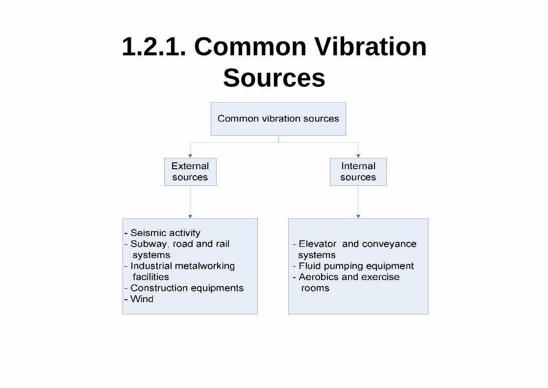
1.2.1. Common Vibration Sources

1.2.2 Forms of Vibration• Free vibration is the natural response of a structure to

some impact or displacement • Forced vibration is the response of a structure to a

repetitive forcing function that causes the structure to vibrate at the frequency of the excitation

• Sinusoidal vibration is a special class of vibration. The structure is excited by a forcing function that is a pure tone with a single frequency

• Random vibration is very common in nature. The vibration you feel when driving a car result from a complex combination of the rough road surface, engine vibration, wind buffeting the car's exterior, etc

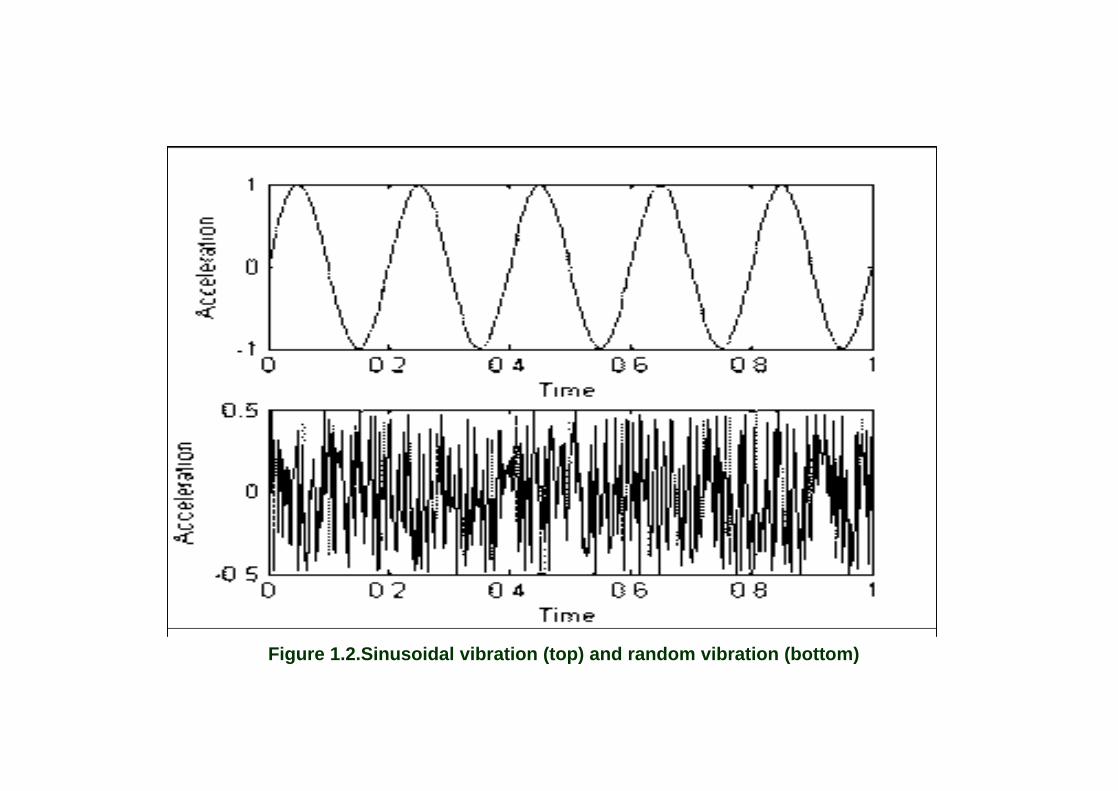
Figure 1.2.Sinusoidal vibration (top) and random vibration (bottom)

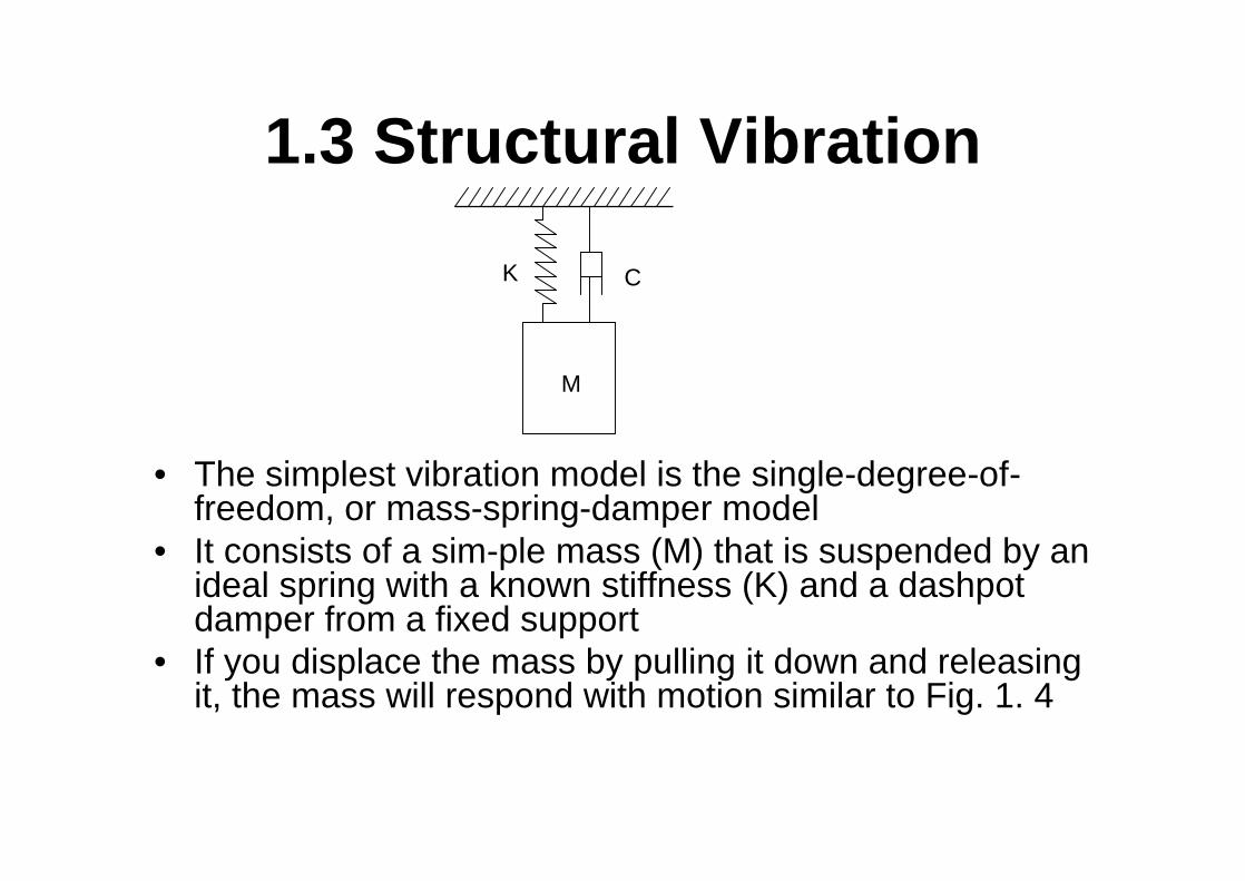
1.3 Structural Vibration

• The simplest vibration model is the single-degree-of-freedom, or mass-spring-damper model

• It consists of a sim-ple mass (M) that is suspended by an ideal spring with a known stiffness (K) and a dashpot damper from a fixed support

• If you displace the mass by pulling it down and releasing it, the mass will respond with motion similar to Fig. 1. 4

M

K C

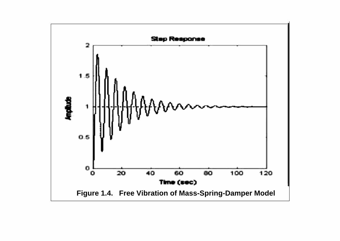
Figure 1.4. Free Vibration of Mass-Spring-Damper Model

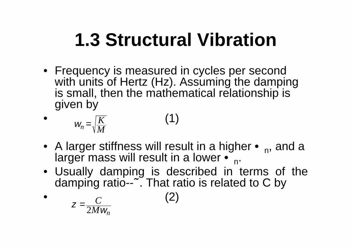
1.3 Structural Vibration• Frequency is measured in cycles per second

with units of Hertz (Hz). Assuming the damping is small, then the mathematical relationship is given by

• (1)

• A larger stiffness will result in a higher •n, and a larger mass will result in a lower •n.

• Usually damping is described in terms of the damping ratio--˜. That ratio is related to C by

• (2)

nKMω =

2 nC

Mζ ω=

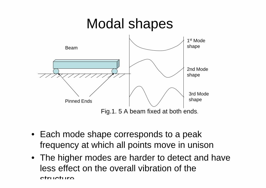
Modal shapes

• Each mode shape corresponds to a peak frequency at which all points move in unison

• The higher modes are harder to detect and have less effect on the overall vibration of the structure.

1st Mode shape

2nd Mode shape

3rd Mode shape

Beam

Pinned Ends

Fig.1. 5 A beam fixed at both ends.

PART II. Vibration of Plates

2.1 General Theory2.2 Transverse Vibration of a rectangular

plate.

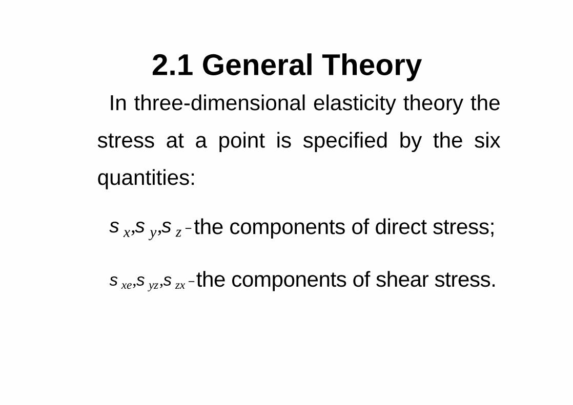
2.1 General TheoryIn three-dimensional elasticity theory the

stress at a point is specified by the six

quantities:

, , zx yσ σ σ − the components of direct stress;

, ,xe yz zxσ σ σ −the components of shear stress.

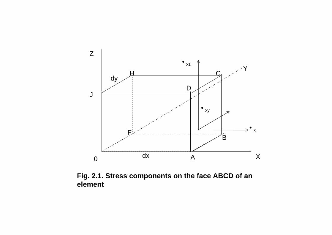
X

Y

•x

0

H C

D

B

A

F

dx

•xy

•xz

J

Z

dy

Fig. 2.1. Stress components on the face ABCD of an element

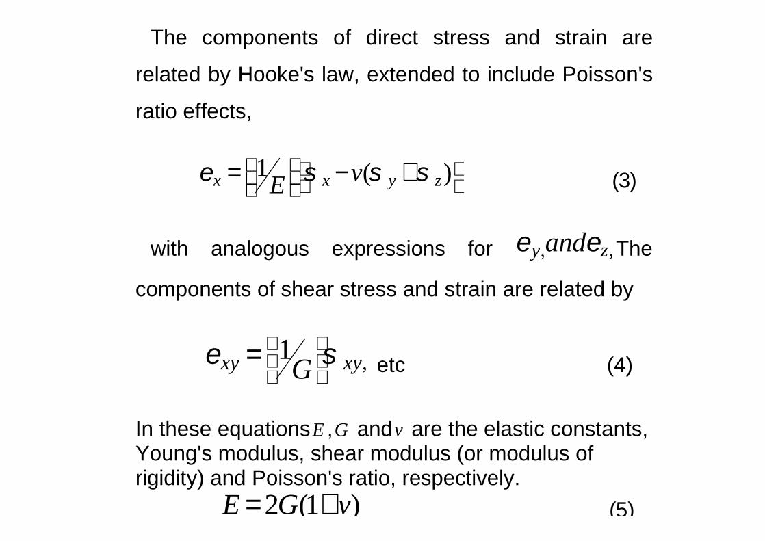
The components of direct stress and strain are

related by Hooke's law, extended to include Poisson's

ratio effects,

1 ( )x x y zvEε σ σ σ = − + (3)

with analogous expressions for ,, zy andε ε The

components of shear stress and strain are related by

,1xy xyGε σ

= etc (4)

In these equationsE ,G andv are the elastic constants, Young's modulus, shear modulus (or modulus of rigidity) and Poisson's ratio, respectively.

2 (1 )E G v= + (5)

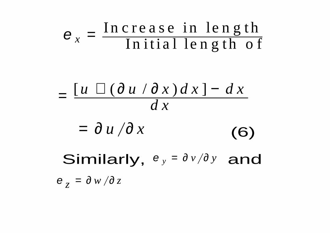
I n c r e a s e i n le n g t h o f e le m e n tI n i t i a l l e n g t h o f e le m e n txε =

[ ( / ) ]u u x d x d xd x

+ ∂ ∂ −=

u x= ∂ ∂ (6)

Similarly, y v yε = ∂ ∂ andw zzε = ∂ ∂

u

˜

•

v

A B

C1

B1

D1

D

A1

xy

X

Y

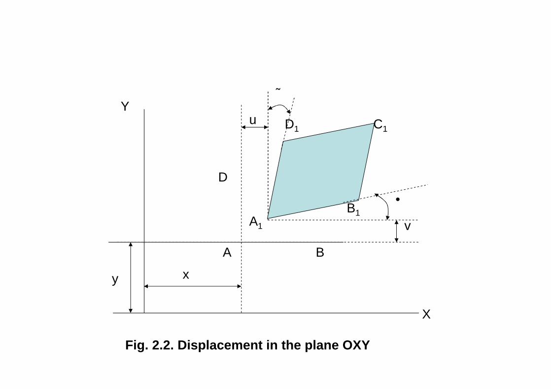
Fig. 2.2. Displacement in the plane OXY

The deformed shape of the element is the

parallelogram A1 B1 C1 D1 and the shear

strain is (a + •). Thus for small angles

xyv ux yε α β ∂ ∂= + = +∂ ∂ (7)

Similarly,

yzw vy zε ∂ ∂= +∂ ∂ and zx

u wz xε ∂ ∂= +∂ ∂

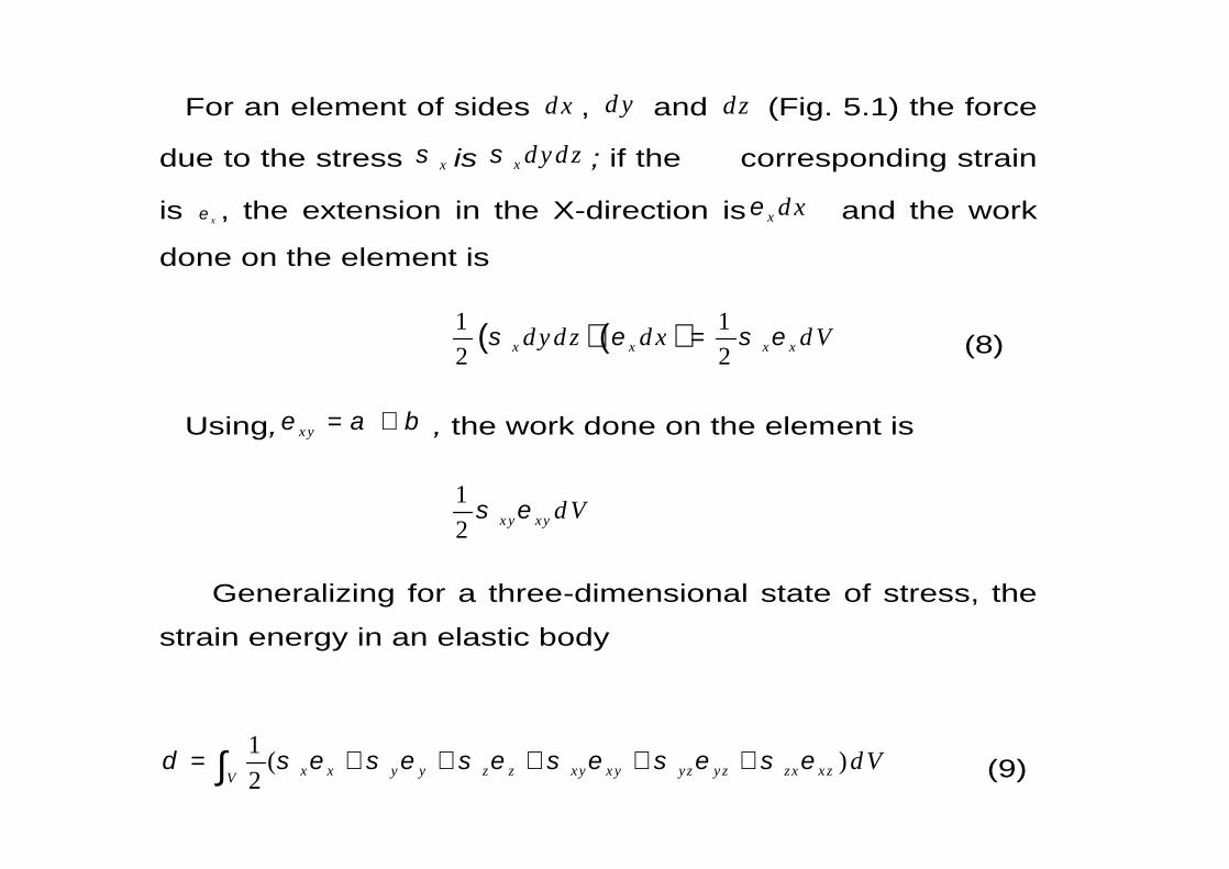
For an element of sides d x , d y and dz (Fig. 5.1) the force

due to the stress xσ is x d y d zσ ; if the corresponding strain

is xε , the extension in the X-direction is x d xε and the work

done on the element is

( )( )1 12 2x x x xd y d z d x d Vσ ε σ ε= (8)

Using, x yε α β= + , the work done on the element is

12 x y xy d Vσ ε

Generalizing for a three-dimensional state of stress, the

strain energy in an elastic body

1 ( )2 x x y y z z xy x y yz y z zx x zV

d Vδ σ ε σ ε σ ε σ ε σ ε σ ε= + + + + +∫ (9)

2.2 Transverse Vibrations of Rectangular Plate

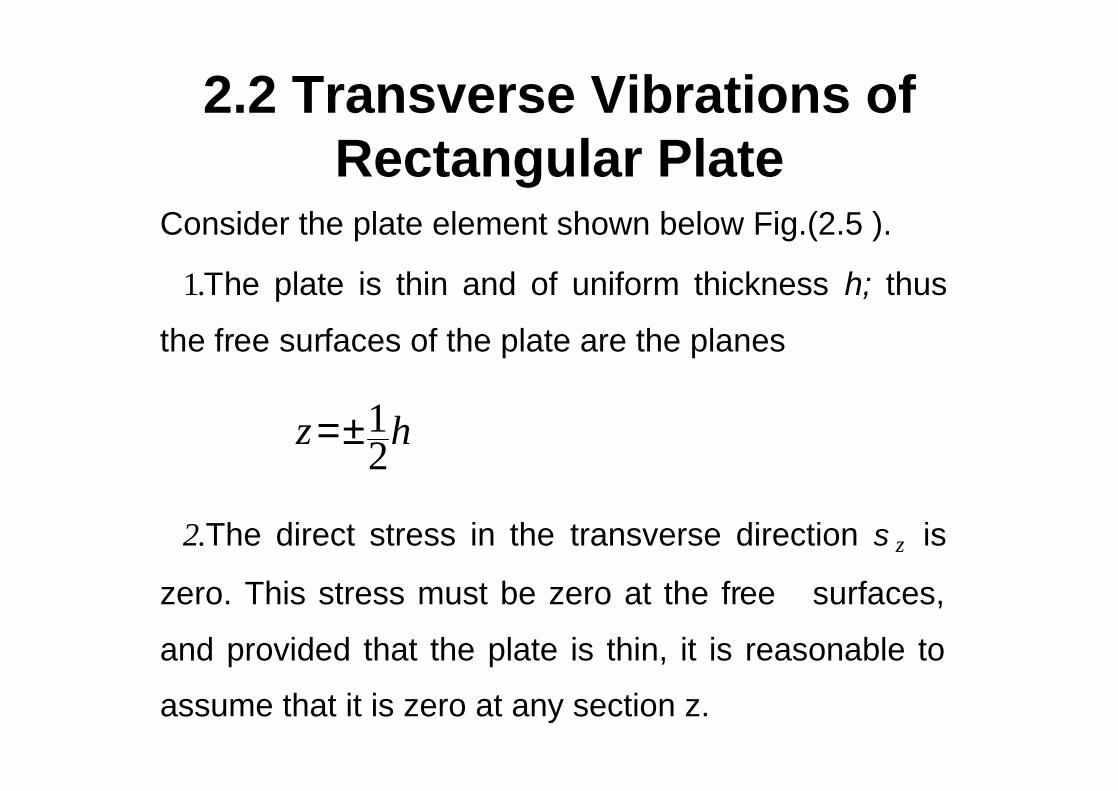
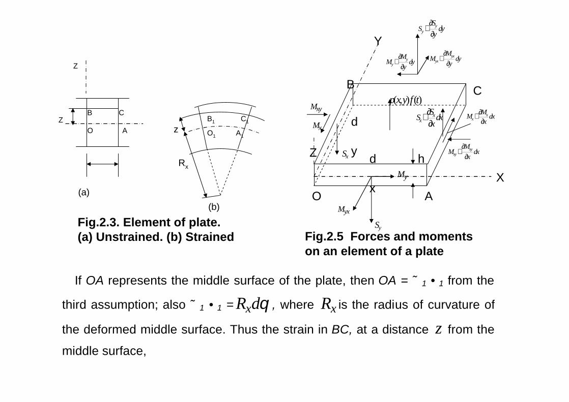
Consider the plate element shown below Fig.(2.5 ).

1.The plate is thin and of uniform thickness h; thus

the free surfaces of the plate are the planes

12z h=±

2.The direct stress in the transverse direction zσ is

zero. This stress must be zero at the free surfaces,

and provided that the plate is thin, it is reasonable to

assume that it is zero at any section z.

˜Stresses in the middle plane of the plate

(membrane stresses) are neglected, i.e. transverse

forces are supported by bending stresses, as in

flexure of a beam.

˜Plane sections that are initially normal to the middle

plane remain plane and normal to it. Thus with this

assumption the shear strains xzσ and yzσ are zero.

˜Only the transverse displacement w (in the Z-

direction) has to be considered.

X

yy

MM dy

y∂

+∂

yyS

Sdy

y∂

+∂

yxyx

MM dy

y∂

+∂

xyxy

MM dx

x∂

+∂

xx

MM dxx

∂+∂

xxS

S dxx

∂+∂

d

x

d

yxS

yS

xM

yxM

xyM

yM

Y

Z

O A

CB( , ) ( )p x y f t

Fig.2.5 Forces and moments on an element of a plate

h

C

AO

B

Z

Z C1

(a)

A1

B1

O1

Rx

z

(b)

Fig.2.3. Element of plate. (a) Unstrained. (b) Strained

If OA represents the middle surface of the plate, then OA = ˜1 •1 from the

third assumption; also ˜1 •1 = xR dθ , where xR is the radius of curvature of

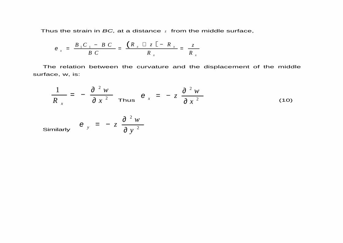
the deformed middle surface. Thus the strain in BC, at a distance z from the

middle surface,

Thus the strain in BC, at a distance z from the middle surface,

1 1 x xx

x x

R z RB C BC zR RBCε

+ −−= = =

The relation between the curvature and the displacement of the middle

surface, w, is:

22

1x

wR x

∂=−∂

Thus

22xwz

xε ∂=−

∂ (10)

Similarly

22ywz

yε ∂= −

∂

Thus the strain in BC, at a distance z from the middle surface,

( )1 1 x x

xx x

R z RB C B C zB C R R

ε+ −−

= = =

The relation between the curvature and the displacement of the middle

surface, w, is:

2

2

1

x

wR x

∂= −

∂ Thus

2

2xwz

xε

∂= −

∂ (10)

Similarly

2

2ywz

yε

∂= −

∂

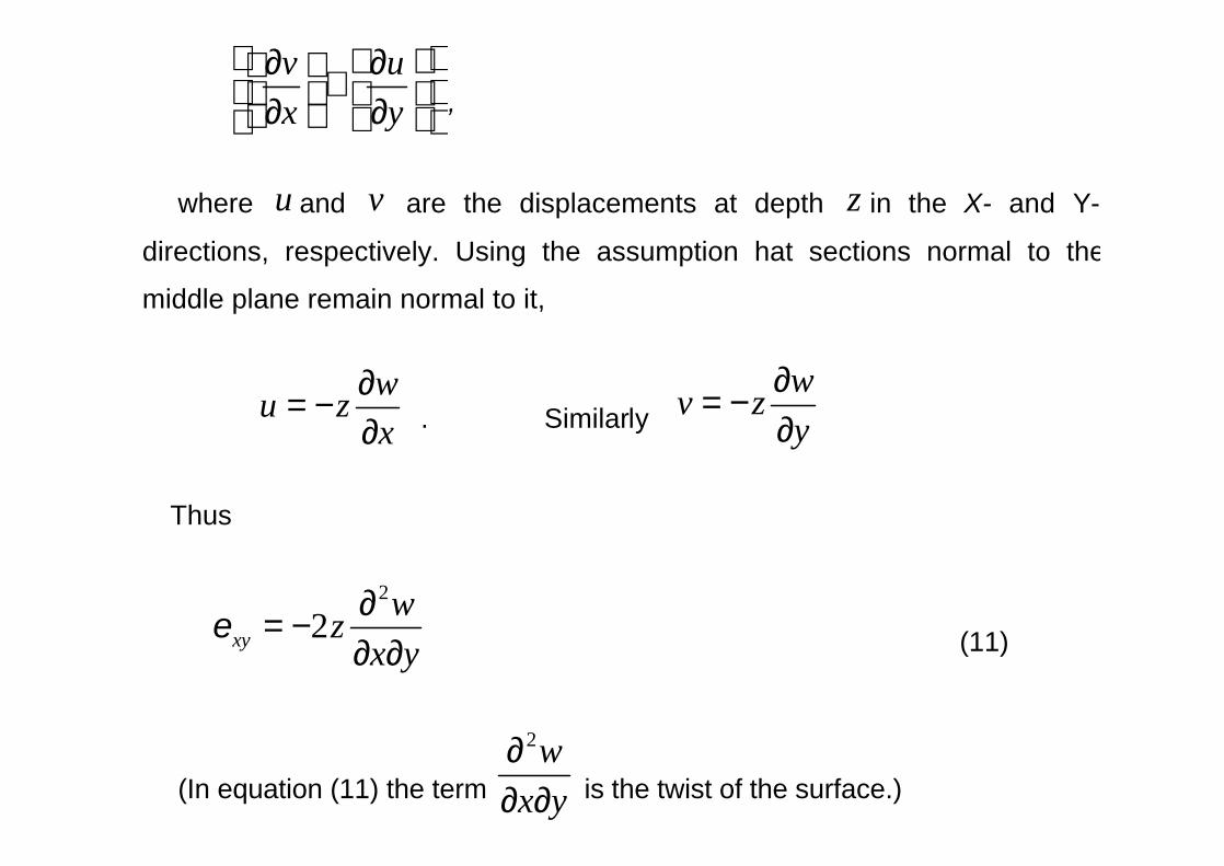
v ux y

∂ ∂ + ∂ ∂ ,

where u and v are the displacements at depth z in the X- and Y-

directions, respectively. Using the assumption hat sections normal to the

middle plane remain normal to it,

wu zx

∂= −

∂ . Similarly wv zy

∂= −

∂

Thus

2

2xywz

x yε

∂= −

∂ ∂ (11)

(In equation (11) the term

2wx y

∂∂ ∂ is the twist of the surface.)

( )21x x yE vv

σ ε ε= +−

( )21y y xE vv

σ ε ε= +−

( )2 1xy xyE

vσ ε=

−

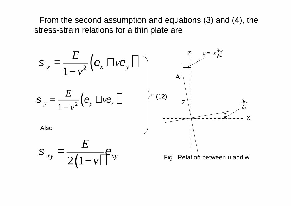
From the second assumption and equations (3) and (4), the stress-strain relations for a thin plate are

(12)

Also

Z

A

Z

X

wu z x∂= −∂

wx

∂∂

Fig. Relation between u and w

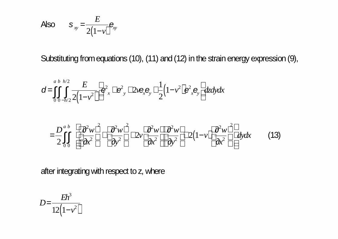
Also ( )2 1xy xyE

vσ ε=

−

Substituting from equations (10), (11) and (12) in the strainenergy expression (9),

( ) ( )/2

2 2 2 22

0 0 /2

12 122 1

a b h

x y x y x yh

E v v dzdydxv

δ ε ε ε ε ε ε−

= + + + − − ∫∫ ∫

( )2 2 22 2 2 2 2

2 2 2 2 20 0

2 2 12

a bD w w w w wv v dydxx y x y x

∂ ∂ ∂ ∂ ∂= + + + − ∂ ∂ ∂ ∂ ∂

∫∫ (13)

after integrating with respect toz, where

( )3

212 1EhD

v=

−

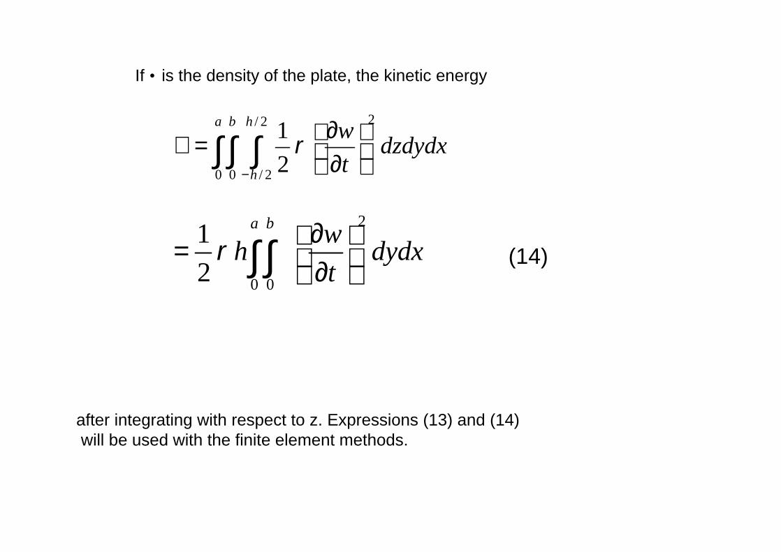
2/ 2

0 0 / 2

12

a b h

h

w dzdydxt

ρ−

∂ ℑ = ∂ ∫ ∫ ∫

2

0 0

12

a b wh dydxt

ρ∂ = ∂ ∫ ∫

If • is the density of the plate, the kinetic energy

after integrating with respect to z. Expressions (13) and (14)will be used with the finite element methods.

(14)

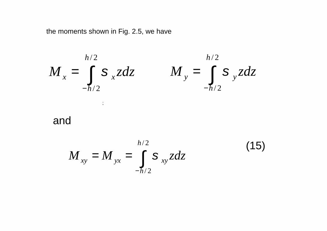
/ 2

/ 2

h

x xh

M zdzσ−

= ∫/ 2

/ 2

h

y yh

M zdzσ−

= ∫

/ 2

/ 2

h

xy yx xyh

M M zdzσ−

= = ∫

the moments shown in Fig. 2.5, we have

;

and

(15)

2

2( , ) ( ) yx SS wp x y f t hx y t

ρ∂∂ ∂

+ + =∂ ∂ ∂

0yxxx

MM Sx y

∂∂+ − =

∂ ∂0y xy

y

M MS

y x∂ ∂

− + + =∂ ∂

2 22 2

2 2 2( , ) ( )xy yx M MM wp x y f t hx x y y t

ρ∂ ∂∂ ∂

+ + + =∂ ∂ ∂ ∂ ∂

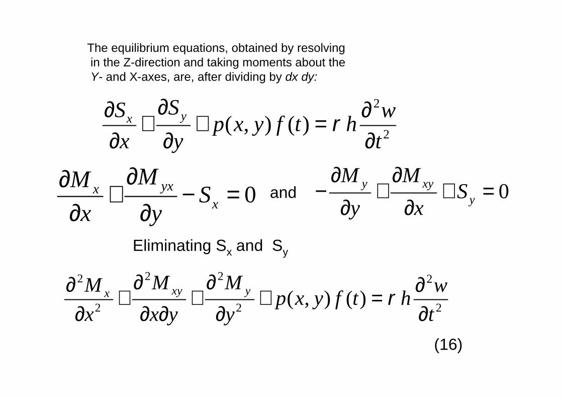
The equilibrium equations, obtained by resolvingin the Z-direction and taking moments about theY- and X-axes, are, after dividing by dx dy:

and

Eliminating Sx and Sy

(16)

2 2

2 2xw wM D v

x y ∂ ∂

= − + ∂ ∂

2 2

2 2yw wM D v

y x ∂ ∂

= − + ∂ ∂

2

(1 ) wMxy D vx y

∂= − −

∂ ∂

w

4 4 4 2

4 2 2 4 22 ( , ) ( )w w w wD h p x y f tx x y y t

ρ ∂ ∂ ∂ ∂

+ + + = ∂ ∂ ∂ ∂ ∂

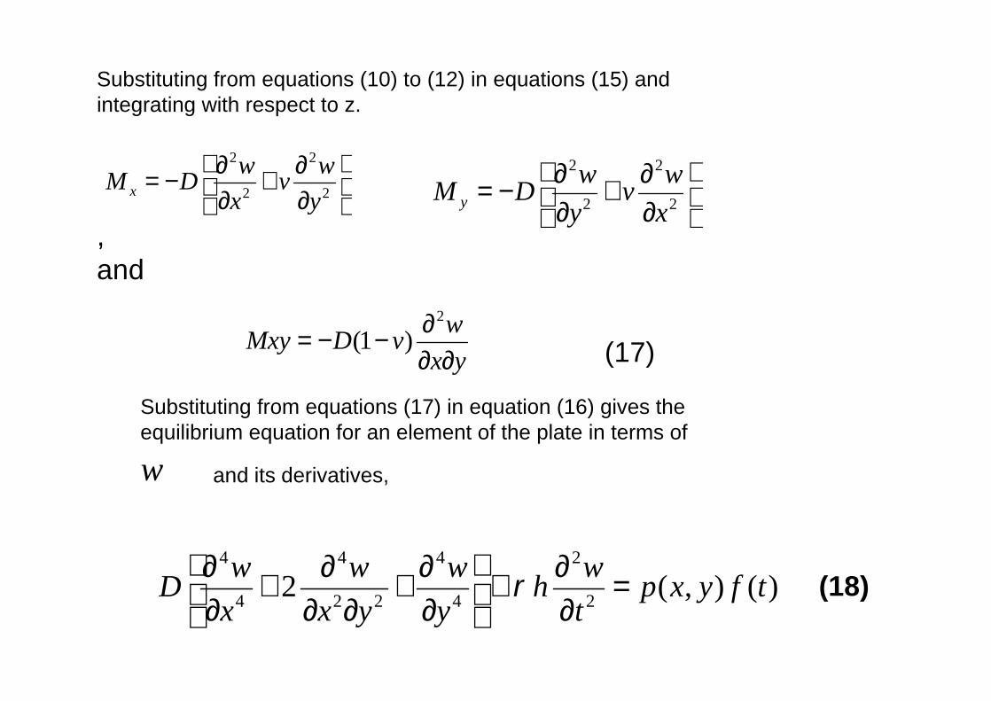
Substituting from equations (10) to (12) in equations (15) and integrating with respect to z.

; , and

Substituting from equations (17) in equation (16) gives the equilibrium equation for an element of the plate in terms of

and its derivatives,

(17)

(18)

PART III. Application of FEM

3.1 Finite Element Method (FEM)3.2 Element Stiffness and Mass Matrices3.2.1 Axial Element3.3 FEM for In-plane Vibration3.4 FEM for Transverse Vibration.

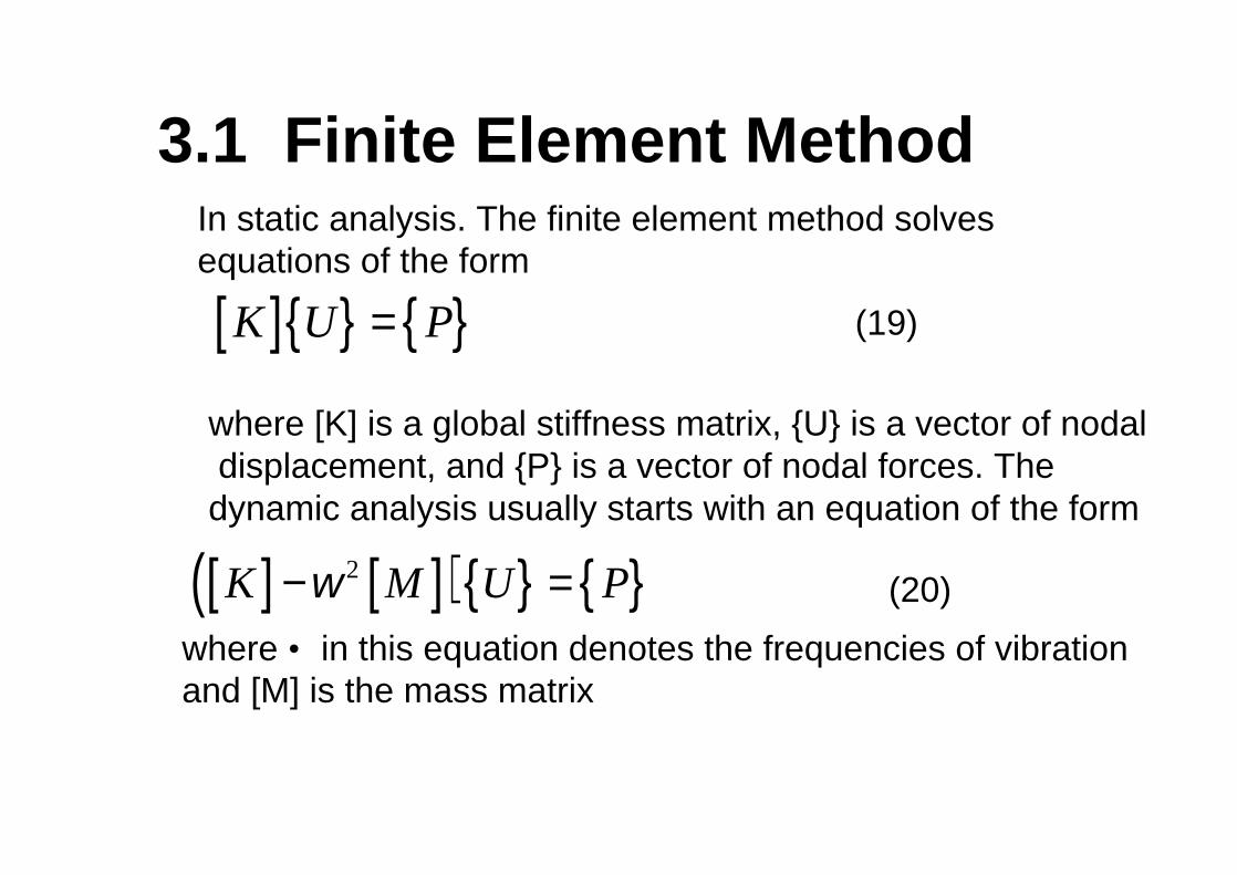
3.1 Finite Element Method

[ ]{ } { }K U P=

[ ] [ ]( ){ } { }2K M U Pω− =

In static analysis. The finite element method solves equations of the form

where [K] is a global stiffness matrix, {U} is a vector of nodaldisplacement, and {P} is a vector of nodal forces. The

dynamic analysis usually starts with an equation of the form

where • in this equation denotes the frequencies of vibration and [M] is the mass matrix

(19)

(20)

[ ] [ ]( ){ } { }2 0K M Uω− =

[ ] [ ]2K Mω=

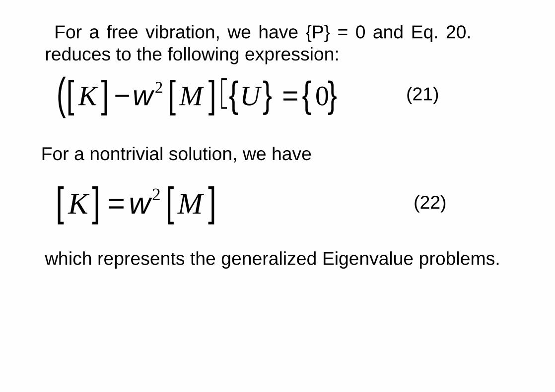
For a free vibration, we have {P} = 0 and Eq. 20. reduces to the following expression:

For a nontrivial solution, we have

(21)

(22)

which represents the generalized Eigenvalue problems.

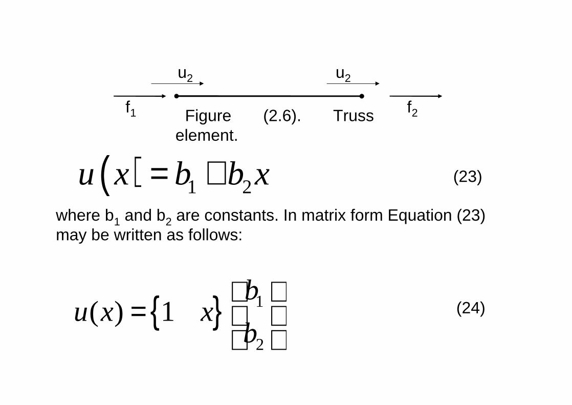
( ) 1 2u x b b x= +

{ } 1

2

( ) 1b

u x xb

=

u2 u2

where b1 and b2 are constants. In matrix form Equation (23) may be written as follows:

(24)

Figure (2.6). Truss element.

f1 f2

(23)

( ) 1 20 (0)u b b= +

( ) 2 2u L b Lb= +

1 1

2 2

1 01

u bu bL

=

1 1

2 2

01 1

b uLb u

= −

1

2

( ) 1ux xu xuL L

= −

{ } 11 2

2

( )u

u x H Hu

=

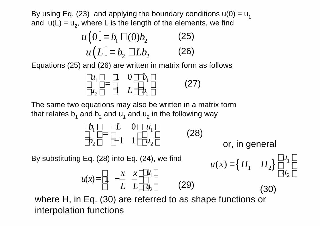
By using Eq. (23) and applying the boundary conditions u(0) = u1and u(L) = u2, where L is the length of the elements, we find

Equations (25) and (26) are written in matrix form as follows

The same two equations may also be written in a matrix form that relates b1 and b2 and u1 and u2 in the following way

By substituting Eq. (28) into Eq. (24), we find

or, in general

where H, in Eq. (30) are referred to as shape functions or interpolation functions

(25)(26)

(27)

(28)

(30)(29)

ε ( )u xx

−=

2

111uu

LLε

εσ E=

The axial strain in Fig 2.7 is the rate change of with respect to

. Therefore, by differentiating Eq. (29) with respect to x, we find

By applying Hooke's law, the normal stress ˜ at cross sectionsalong the length of the element is given by the expression

where • is Young's modulus of elasticity and ˜ is given by Eq. (31).

(30)

(31)

∏

221102

1 ufufdxdxdu

dxduEA

TL

−−

=∏ ∫

{ } { }

−

−

−=∏ ∫

2

121

2

1

021

111

1

21

uu

ffdxuu

LLL

LuuEAL

∫ =L

Ldx0

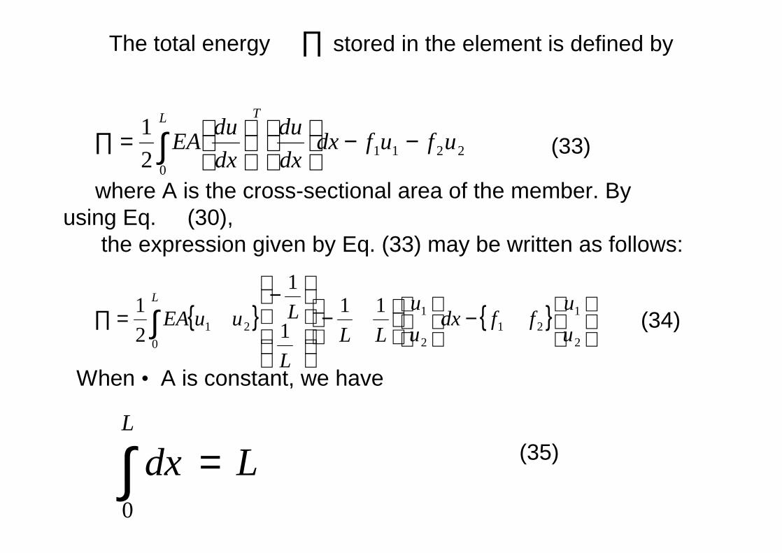
The total energy stored in the element is defined by

where A is the cross-sectional area of the member. By using Eq. (30),

the expression given by Eq. (33) may be written as follows:

When • A is constant, we have

(35)

(33)

(34)

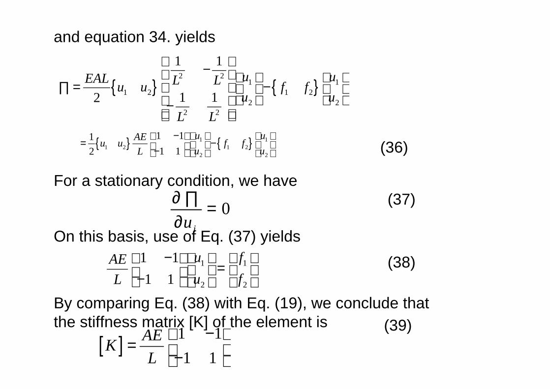
{ } { }2 2

1 11 2 1 2

2 22 2

1 1

1 12u uEAL L Lu u f fu u

L L

− ∏ = −

−

{ } { }1 11 2 1 2

2 2

1 111 12

u uAEu u f fu uL

− = − −

0iu

∂ ∏=

∂

1 1

2 2

1 11 1

u fAEu fL

− = −

[ ] 1 11 1

AEKL

− = −

and equation 34. yields

For a stationary condition, we have

On this basis, use of Eq. (37) yields

By comparing Eq. (38) with Eq. (19), we conclude that the stiffness matrix [K] of the element is

(36)

(37)

(38)

(39)

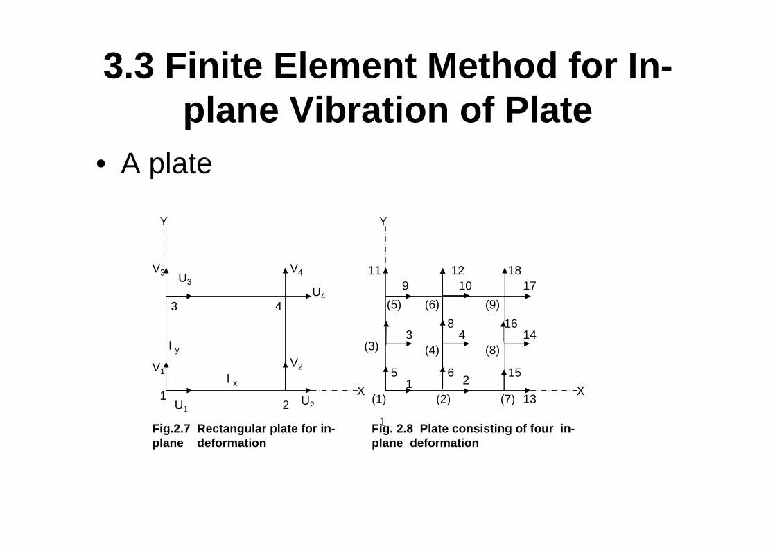
3.3 Finite Element Method for In-plane Vibration of Plate

• A plate

Y

X

V3

V1

Fig.2.7 Rectangular plate for in-plane deformation

Y

X

1

(5) (9)(6)17

18

1

(8)

Fig. 2.8 Plate consisting of four in-plane deformation

5

3

(1) (2) (7)

(3) (4)

6 2 15

13

84

1614

119

1210

1

3 4

2

U3U4

V4

U1U2

V2l x

l y

0 0

1 ( )2

y xl l

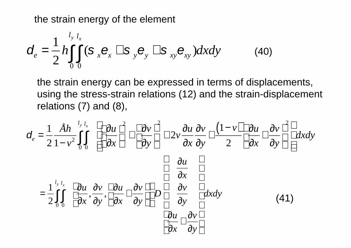
e x x y y xy xyh dxdyδ σ ε σ ε σ ε= + +∫ ∫

( )2 22

20 0

11 22 1 2

y xl l

e

vÅh u v u v u vv dxdyv x y x y x y

δ − ∂ ∂ ∂ ∂ ∂ ∂ = + + + + − ∂ ∂ ∂ ∂ ∂ ∂

∫ ∫

0 0

1 , ,2

y xl l

ux

u v u v vD dxdyx y x y y

u vx y

∂

∂ ∂ ∂ ∂ ∂ ∂

= + ∂ ∂ ∂ ∂ ∂ ∂ ∂

+ ∂ ∂

∫ ∫

the strain energy of the element

the strain energy can be expressed in terms of displacements,using the stress-strain relations (12) and the strain-displacementrelations (7) and (8),

(41)

(40)

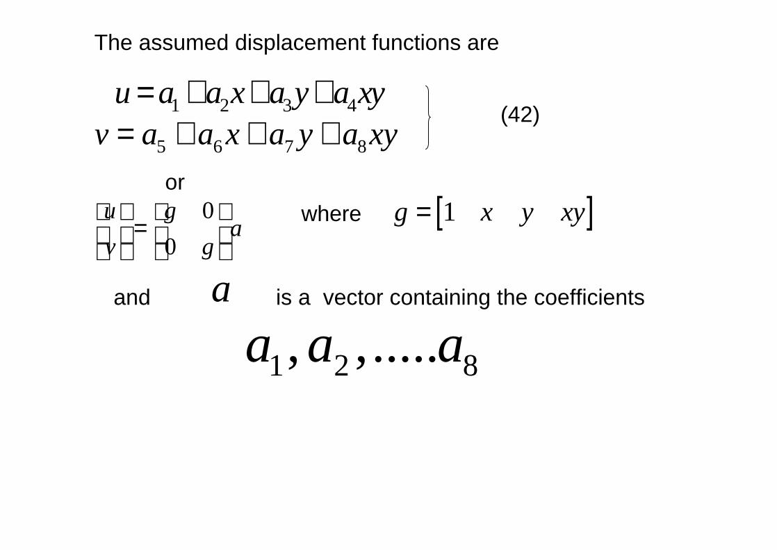
1 2 3 4u a a x a y a xy= + + +5 6 7 8v a a x a y a xy= + + +

00

u ga

v g

=

[ ]1g x y xy=

a

1 2 8, ,.....a a a

The assumed displacement functions are

(42)

where

and is a vector containing the coefficients

or

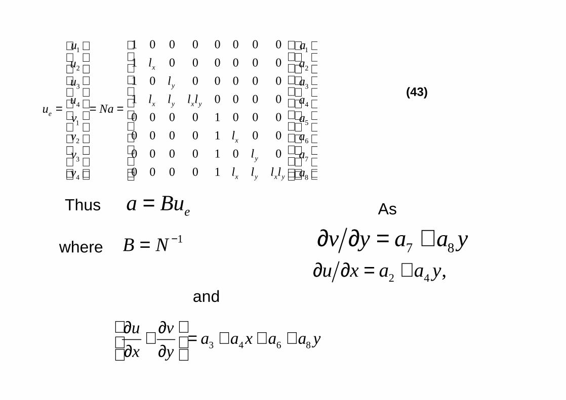
11

22

33

44

51

62

73

84

1 0 0 0 0 0 0 01 0 0 0 0 0 01 0 0 0 0 0 01 0 0 0 00 0 0 0 1 0 0 00 0 0 0 1 0 00 0 0 0 1 0 00 0 0 0 1

x

y

x y x ye

x

y

x y x y

aul au

l aul l l l au

u Naav

l avl av

l l l l av

= = =

ea Bu=1B N −=

2 4 ,u x a a y∂ ∂ = +7 8v y a a y∂ ∂ = +

3 4 6 8u v a a x a a yx y

∂ ∂+ = + + + ∂ ∂

Thus

where

As

and

(43)

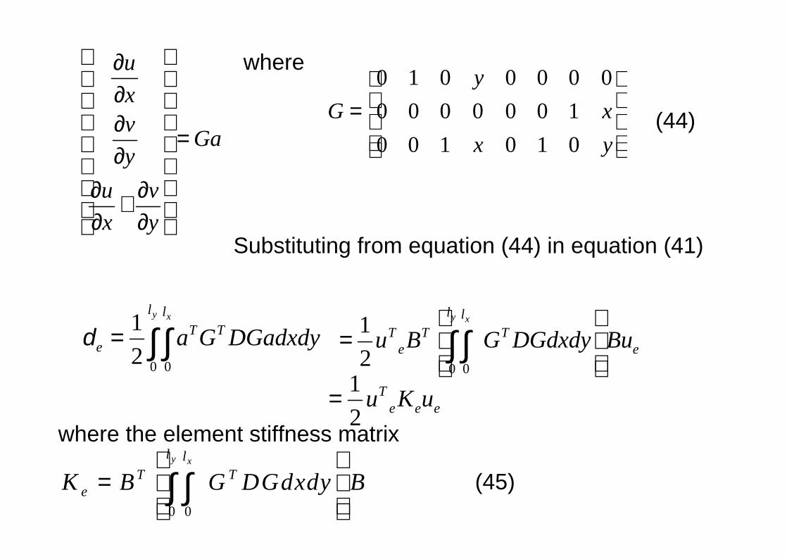
uxv Gay

u vx y

∂

∂ ∂

= ∂ ∂ ∂

+ ∂ ∂

0 1 0 0 0 0 00 0 0 0 0 0 10 0 1 0 1 0

yG x

x y

=

0 0

12

y xl lT T

e a G DGadxdyδ = ∫ ∫0 0

12

y xl lT T T

e eu B G DGdxdy Bu

= ∫ ∫

12

Te e eu K u=

0 0

y xl lT T

eK B G DGdxdy B

= ∫ ∫

where

Substituting from equation (44) in equation (41)

where the element stiffness matrix

(44)

(45)

2 2

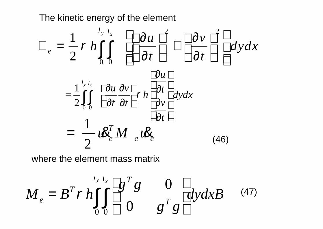
0 0

12

y xl l

eu vh dydxt t

ρ ∂ ∂ ℑ = + ∂ ∂

∫ ∫

0 0

12

y xl lu

u v th dydxvt tt

ρ

∂ ∂ ∂ ∂= ∂∂ ∂ ∂

∫ ∫

12

Te e eu M u= & &

0 0

00

y xl l TT

e T

g gM B h dydxB

g gρ

=

∫ ∫

The kinetic energy of the element

where the element mass matrix

(46)

(47)

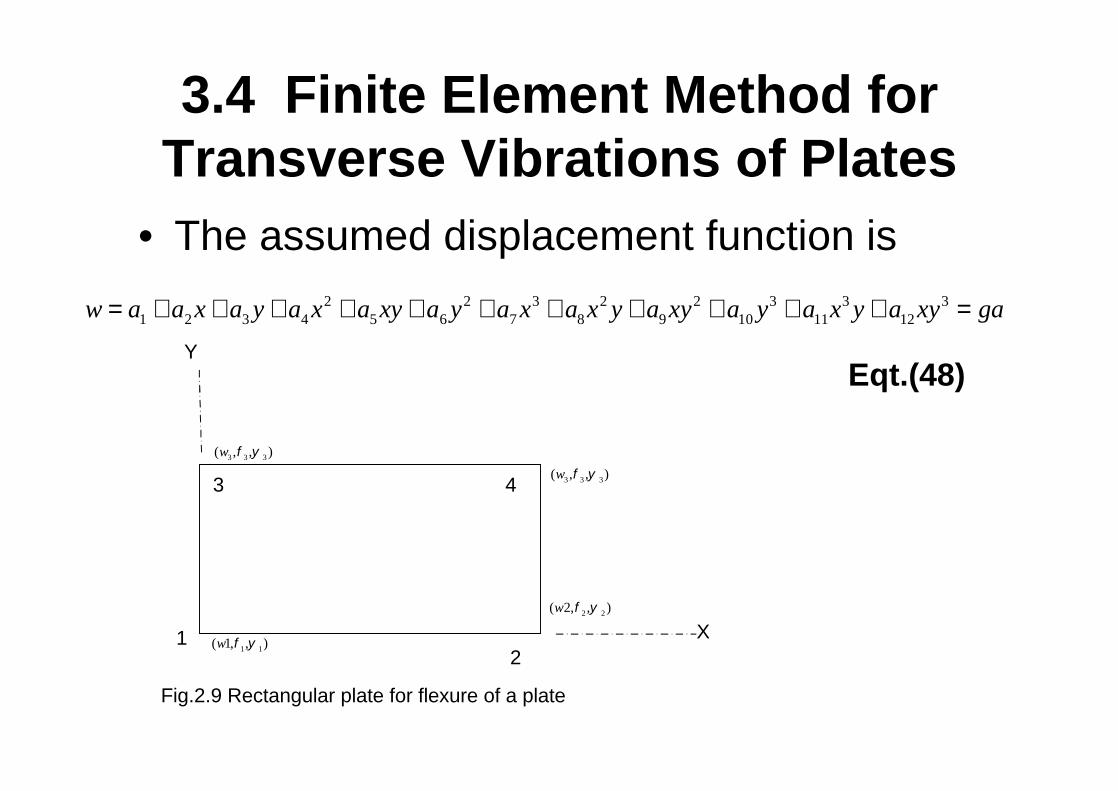
3.4 Finite Element Method for Transverse Vibrations of Plates

• The assumed displacement function is

Y

X1

3 4

2

Fig.2.9 Rectangular plate for flexure of a plate

3 3 3( , , )w φ ψ

1 1( 1, , )w φ ψ

2 2( 2, , )w φ ψ

3 3 3( , , )w φ ψ

2 2 3 2 2 3 3 31 2 3 4 5 6 7 8 9 10 11 12w a a x a y a x a xy a y a x a x y a xy a y a x y a xy ga= + + + + + + + + + + + =

Eqt.(48)

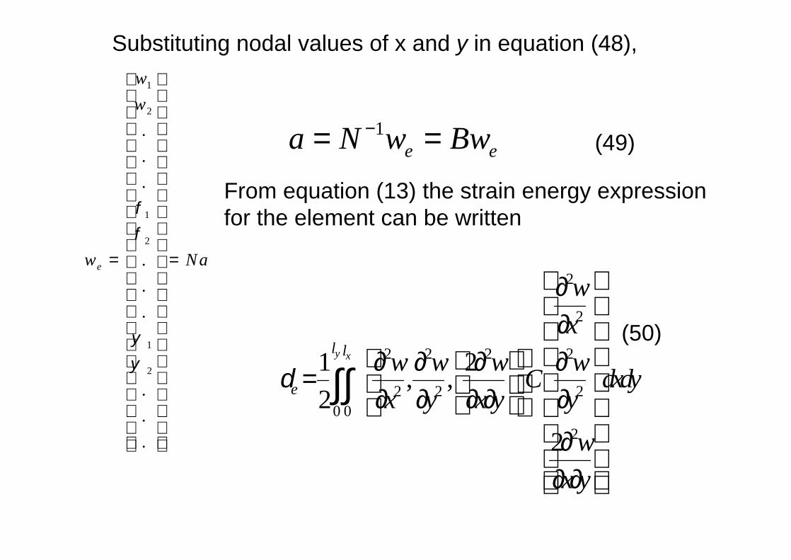
Substituting nodal values of x and y in equation (48),1

2

1

2

1

2

.

.

.

.

.

.

.

.

.

e

ww

w Na

φφ

ψψ

= =

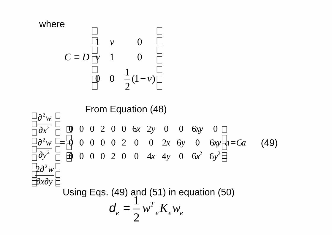
1e ea N w Bw−= =

2

2

2 2 2 2

2 2 20 0

2

1 2, ,2

2

y xl l

e

wx

w w w wC dxdyx y x y y

wx y

δ

∂

∂ ∂ ∂ ∂ ∂

= ∂ ∂ ∂ ∂ ∂ ∂ ∂ ∂

∫∫

From equation (13) the strain energy expression for the element can be written

(50)

(49)

1 01 0

10 0 (1 )2

vC D v

v

=

−

2

2

2

2

22

wxw

yw

x y

∂

∂ ∂

∂ ∂

∂ ∂

2 2

0 0 0 2 0 0 6 2 0 0 6 00 0 0 0 0 2 0 0 2 6 0 60 0 0 0 2 0 0 4 4 0 6 6

x y xyx y xy a Ga

x y x y

= =

12

Te e e ew K wδ =

where

From Equation (48)

Using Eqs. (49) and (51) in equation (50)

(49)

0 0

y xl lT T

eK B G CGdxdy B

= ∫ ∫

2

0 0

12

y xl l

ewh dydxt

ρ∂ ℑ = ∂ ∫ ∫

ew gBwt

∂=

∂&

12

Te e e ew M wℑ = & &

0 0

y xl lT T

eM B h g dydx Bρ

=

∫ ∫

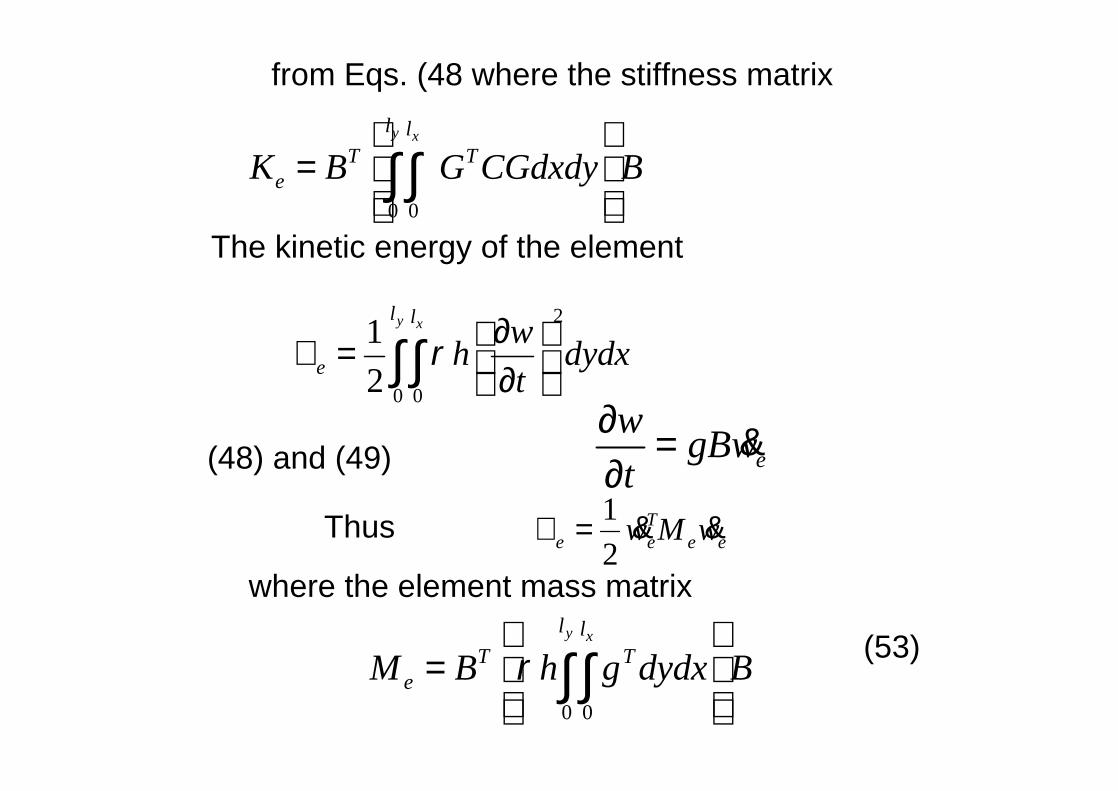
from Eqs. (48 where the stiffness matrix

The kinetic energy of the element

(48) and (49)

Thus

where the element mass matrix

(53)

For forced vibration the matrix equation

Mw Kw p+ =&& (54)

( , ) ( )p x y f t

0 0

( , ) ( ) ( , )y xl l

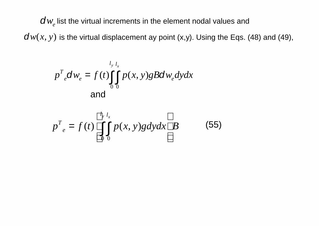
Te ep w p x y f t w x y dydxδ δ=∫∫

Considering the con-tribution to p from a particularelement, pe, and supposing that this element is

subjected to a transverse applied force per unit area of

,application of the principle of virtual work gives.

( , )w x yδ

0 0

( ) ( , )y xl l

Te e ep w f t p x y gB w dydxδ δ= ∫ ∫

0 0

( ) ( , )y xl l

Tep f t p x y gdydx B

=

∫ ∫

list the virtual increments in the element nodal values and

is the virtual displacement ay point (x,y). Using the Eqs. (48) and (49),

and

(55)

ewδ

PART IV.

• References • Demeter G. Fertis – “Mechanical and

Structural Vibration.• J. F. Hall - “Finite Element Analysis in

Earthquake Engineering to the international handbook of Earthquake Engineering and Engineering Seismology part B, 2003 .

• G. D.Manolis and D.E. Beskos - Boundary Element Method in Elastodynamics, 1988.