machine vibration basic

Chapter 23

Machine vibration measurement

Unlike most process measurements, the measurement of a rotating machine’s vibration is primarilyfor the benefit of the process equipment rather than the process itself. Vibration monitoring on anammonia vapor compressor, for instance, may very well be useful in extending the operating life ofthe compressor, but it offers little benefit to the control of the ammonia vapor.

Nevertheless, the prevalence of machine vibration measurement technology is so widespreadin the process industries that it cannot be overlooked by the instrument technician. Rotatingmachinery equipped with vibration sensors are often controlled by protection equipment designedto automatically shut down the machine in the event of excessive vibration. The configuration andmaintenance of this protection equipment, and the sensors feeding vibration data to it, is often thedomain of instrument technicians.

23.1 Vibration physics

One very convenient feature of waves is that their properties are universal. Waves of water in theocean, sound waves in air, electronic signal waveforms, and even waves of mechanical vibration mayall be expressed in mathematical form using the trigonometric sine and cosine functions. This meansthe same tools (both mathematical and technological) may be applied to the analysis of differentkinds of waves. A strong example of this is the Fourier Transform, used to determine the frequencyspectrum of a waveform, which may be applied with equal validity to any kind of wave1.

1The “spectrum analyzer” display often seen on high-quality audio reproduction equipment such as stereo equalizersand amplifiers is an example of the Fourier Transform applied to music. This exact same technology may be appliedto the analysis of a machine’s vibration to indicate sources of vibration, since different components of a machine tendto generate vibratory waves of differing frequencies.

1467

shimon

Tony Lesson

1468 CHAPTER 23. MACHINE VIBRATION MEASUREMENT

23.1.1 Sinusoidal vibrations

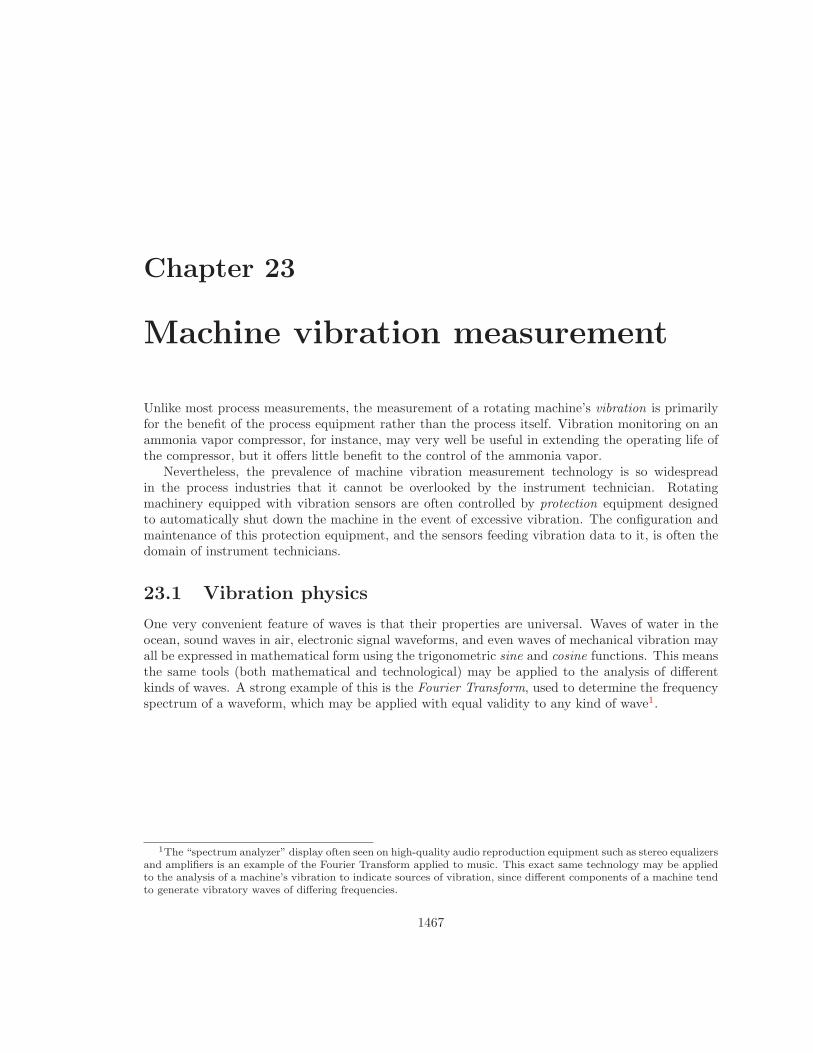
If a rotating wheel is unbalanced by the presence of an off-center mass, the resulting vibration willtake the form of a cosine wave as measured by a displacement (position) sensor near the peripheryof the object (assuming an angle of zero is defined by the position of the displacement sensor). Thedisplacement sensor measures the air gap between the sensor tip and the rim of the spinning wheel,generating an electronic signal (most likely a voltage) directly proportional to that gap:

Off-center mass

Displacement sensor

wires

Rotating wheel

TimeDisplacement

Cosine waveNear

Far

Since the wheel’s shaft “bows” in the direction of the off-center mass as it spins, the gap betweenthe wheel and the sensor will be at a minimum at 0o, and maximum at 180o.

23.1. VIBRATION PHYSICS 1469

We may begin to express this phenomenon mathematically using the cosine function:

x = D cos ωt + b

Where,x = Displacement as measured by sensor at time tD = Peak displacement amplitudeω = Angular velocity (typically expressed in units of radians per second)b = “Bias” air gap measured with no vibrationt = Time (seconds)

Since the cosine function alternates between extreme values of +1 and -1, the constant D isnecessary in the formula as a coefficient relating the cosine function to peak displacement. Thecosine function’s argument (i.e. the angle given to it) deserves some explanation as well: the productωt is the multiple of angular velocity and time, angular velocity typically measured in radians persecond and time typically measured in seconds. The product ωt, then, has a unit of radians. Attime=0 (when the mass is aligned with the sensor), the product ωt is zero and the cosine’s value is+1.

For a wheel spinning at 1720 RPM (approximately 180.1 radians per second), the angle betweenthe off-center mass and the sensor will be as follows:

Time Angle (radians) Angle (degrees) cos ωt0 ms 0 rad 0o +1

8.721 ms π2 rad 90o 0

17.44 ms π rad 180o -126.16 ms 3π

2 rad 270o 034.88 ms 0 rad 360o or 0o +1

We know from physics that velocity is the time-derivative of displacement. That is, velocity isdefined as the rate at which displacement changes over time. Mathematically, we may express thisrelationship using the calculus notation of the derivative:

v =dx

dtor v =

d

dt(x)

Where,v = Velocity of an objectx = Displacement (position) of an objectt = Time


Since we happen to know the equation describing displacement (x) in this system, we maydifferentiate this equation to arrive at an equation for velocity:

v =dx

dt=

d

dt(D cos ωt + b)

Applying the differentiation rule that the derivative of a sum is the sum of the derivatives:

v =d

dt(D cos ωt) +

d

dtb

Recall that D, ω, and b are all constants in this equation. The only variable here is t, whichwe are differentiating with respect to. We know from calculus that the derivative of a simple cosinefunction is a negative sine ( d

dxcos x = − sin x), and that the presence of a constant multiplier in the

cosine’s argument results in that multiplier applied to the entire derivative2 ( ddx

cos ax = −a sin ax).

We also know that the derivative of any constant is simply zero ( ddx

C = 0), which eliminates the bterm:

v = −ωD sinωt

What this equation tells us is that for any given amount of peak displacement (D), the velocityof the wheel’s “wobble” increases linearly with speed (ω). This should not surprise us, since weknow an increase in rotational speed would mean the wheel displaces the same vibrating distance inless time, which would necessitate a higher velocity of vibration.

We may take the process one step further by differentiating the equation again with respect totime in order to arrive at an equation describing the vibrational acceleration of the wheel’s rim,since we know acceleration is the time-derivative of velocity (a = dv

dt):

a =dv

dt=

d

dt(−ωD sin ωt)

From calculus, we know that the derivative of a sine function is a cosine function ( ddx

sin x =cos x), and the same rule regarding constant multipliers in the function’s argument applies here aswell ( d

dxsin ax = a cos ax):

a = −ω2D cos ωt

What this equation tells us is that for any given amount of peak displacement (D), theacceleration of the wheel’s “wobble” increases with the square of the speed (ω). This is of greatimportance to us, since we know the lateral force imparted to the wheel (and shaft) is proportionalto the lateral acceleration and also the mass of the wheel, from Newton’s Second Law of Motion:

F = ma

2This rule makes intuitive sense as well: if a sine or cosine wave increases frequency while maintaining a constantpeak-to-peak amplitude, the rate of its rise and fall must increase as well, since the higher frequency represents lesstime (shorter period) for the wave to travel the same amplitude. Since the derivative is the rate of change of thewaveform, this means the derivative of a waveform must increase with that waveform’s frequency.


Therefore, the vibrational force experienced by this wheel grows rapidly as rotational speedincreases:

F = ma = −mω2D cos ωt

This is why vibration can be so terribly destructive to rotating machinery. Even a small amountof lateral displacement caused by a mass imbalance or other effect may generate enormous forceson the rotating part(s), and these forces grow with the square of the rotating speed (e.g. doublingthe speed quadruples the force; tripling the speed increases force by 9 times). Worse yet, thesecalculations assume a constant displacement (D), which we know will also increase with speedowing to the increased centrifugal force pulling the off-center mass away from the shaft centerline.In practice, doubling or tripling an imbalanced machine’s speed may multiply vibrational forces wellin excess of four or nine times, respectively.

In the United States, it is customary to measure vibrational displacement (D) in units of mils,with one “mil” being 1

1000 of an inch (0.001 inch). Vibrational velocity is measured in inches persecond, following the displacement unit of the inch. Acceleration, although it could be expressedin units of inches per second squared, is more often represented in the unit of the G : a multiple ofEarth’s own gravitational acceleration.

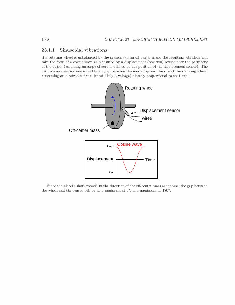
To give perspective to these units, it is helpful to consider a real application. Suppose we have arotating machine vibrating in a sinusoidal (sine- or cosine-shaped) manner with a peak displacement(D) of 2 mils (0.002 inch) at a rotating speed of 1720 RPM (revolutions per minute). The frequencyof this rotation is 28.667 Hz (revolutions per second), or 180.1 radians per second:

Time

f = 1720 RPM = 28.667 Hz

T = 34.88 ms

D = 0.002 in

ω = 2πf = 180.1 rad/s


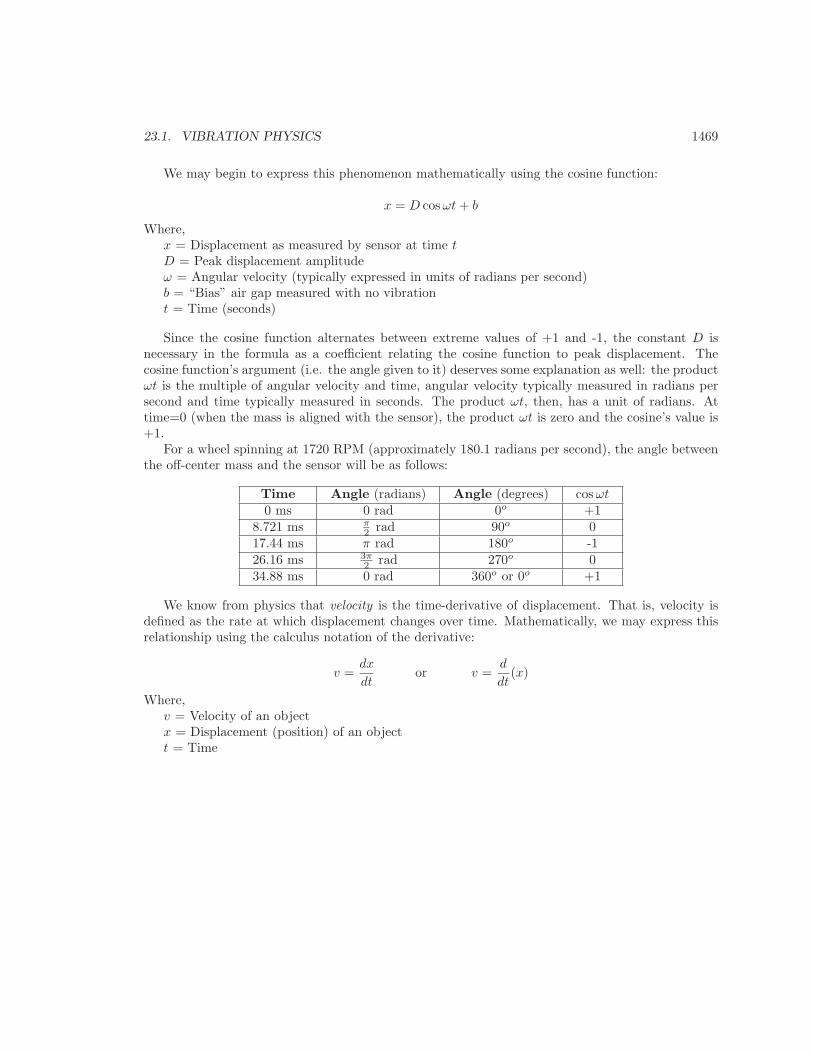
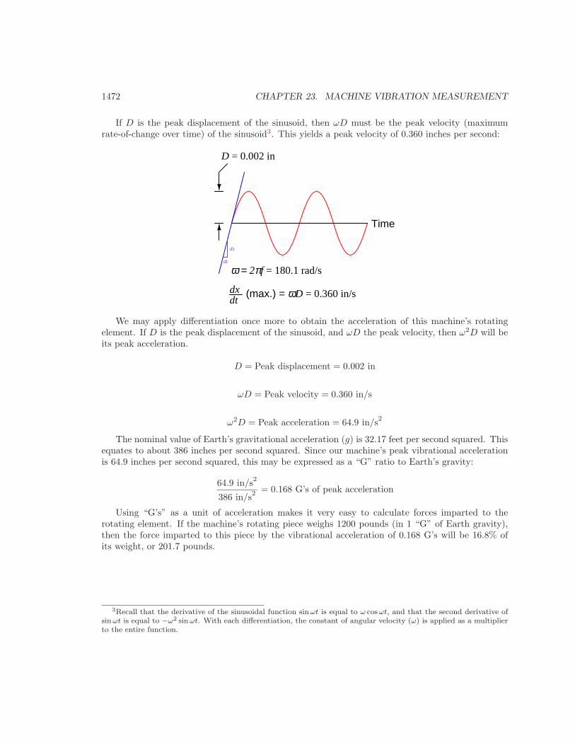
If D is the peak displacement of the sinusoid, then ωD must be the peak velocity (maximumrate-of-change over time) of the sinusoid3. This yields a peak velocity of 0.360 inches per second:

Time

D = 0.002 in

ω = 2πf = 180.1 rad/s

dxdt

(max.) = ωD = 0.360 in/s

dx

dt

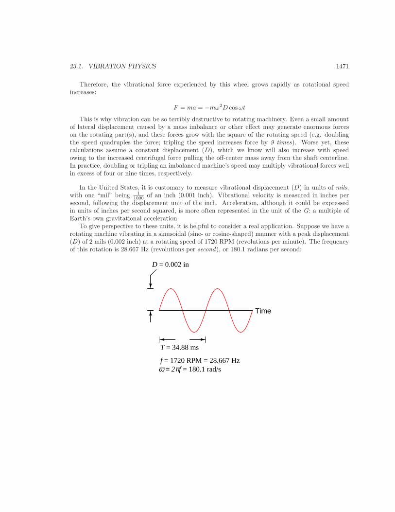
We may apply differentiation once more to obtain the acceleration of this machine’s rotatingelement. If D is the peak displacement of the sinusoid, and ωD the peak velocity, then ω2D will beits peak acceleration.

D = Peak displacement = 0.002 in

ωD = Peak velocity = 0.360 in/s

ω2D = Peak acceleration = 64.9 in/s2

The nominal value of Earth’s gravitational acceleration (g) is 32.17 feet per second squared. Thisequates to about 386 inches per second squared. Since our machine’s peak vibrational accelerationis 64.9 inches per second squared, this may be expressed as a “G” ratio to Earth’s gravity:

64.9 in/s2

386 in/s2 = 0.168 G’s of peak acceleration

Using “G’s” as a unit of acceleration makes it very easy to calculate forces imparted to therotating element. If the machine’s rotating piece weighs 1200 pounds (in 1 “G” of Earth gravity),then the force imparted to this piece by the vibrational acceleration of 0.168 G’s will be 16.8% ofits weight, or 201.7 pounds.

3Recall that the derivative of the sinusoidal function sin ωt is equal to ω cos ωt, and that the second derivative ofsin ωt is equal to −ω2 sin ωt. With each differentiation, the constant of angular velocity (ω) is applied as a multiplierto the entire function.


23.1.2 Non-sinusoidal vibrations

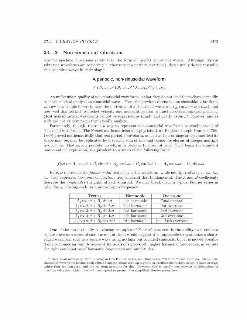
Normal machine vibrations rarely take the form of perfect sinusoidal waves. Although typicalvibration waveforms are periodic (i.e. they repeat a pattern over time), they usually do not resemblesine or cosine waves in their shape:

A periodic, non-sinusoidal waveform

An unfortunate quality of non-sinusoidal waveforms is that they do not lend themselves as readilyto mathematical analysis as sinusoidal waves. From the previous discussion on sinusoidal vibrations,we saw how simple it was to take the derivative of a sinusoidal waveform ( d

dtsin ωt = ω cos ωt), and

how well this worked to predict velocity and acceleration from a function describing displacement.Most non-sinusoidal waveforms cannot be expressed as simply and neatly as sinωt, however, and assuch are not as easy to mathematically analyze.

Fortunately, though, there is a way to represent non-sinusoidal waveforms as combinations ofsinusoidal waveforms. The French mathematician and physicist Jean Baptiste Joseph Fourier (1768-1830) proved mathematically that any periodic waveform, no matter how strange or asymmetrical itsshape may be, may be replicated by a specific sum of sine and cosine waveforms of integer-multiplefrequencies. That is, any periodic waveform (a periodic function of time, f(ωt) being the standardmathematical expression) is equivalent to a series of the following form4:

f(ωt) = A1 cos ωt + B1 sin ωt + A2 cos 2ωt + B2 sin 2ωt + · · ·An cos nωt + Bn sinnωt

Here, ω represents the fundamental frequency of the waveform, while multiples of ω (e.g. 2ω, 3ω,4ω, etc.) represent harmonic or overtone frequencies of that fundamental. The A and B coefficientsdescribe the amplitudes (heights) of each sinusoid. We may break down a typical Fourier series intable form, labeling each term according to frequency:

Terms Harmonic OvertoneA1 cos ωt + B1 sinωt 1st harmonic Fundamental

A2 cos 2ωt + B2 sin 2ωt 2nd harmonic 1st overtoneA3 cos 3ωt + B3 sin 3ωt 3rd harmonic 2nd overtoneA4 cos 4ωt + B4 sin 4ωt 4th harmonic 3rd overtoneAn cos nωt + Bn sinnωt nth harmonic (n − 1)th overtone

One of the most visually convincing examples of Fourier’s theorem is the ability to describe asquare wave as a series of sine waves. Intuition would suggest it is impossible to synthesize a sharp-edged waveform such as a square wave using nothing but rounded sinusoids, but it is indeed possibleif one combines an infinite series of sinusoids of successively higher harmonic frequencies, given justthe right combination of harmonic frequencies and amplitudes.

4There is an additional term missing in this Fourier series, and that is the “DC” or “bias” term A0. Many non-sinusoidal waveforms having peak values centered about zero on a graph or oscilloscope display actually have averagevalues that are non-zero, and the A0 term accounts for this. However, this is usually not relevant in discussions ofmachine vibration, which is why I have opted to present the simplified Fourier series here.


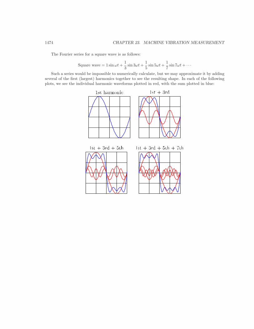
The Fourier series for a square wave is as follows:

Square wave = 1 sin ωt +1

3sin 3ωt +

1

5sin 5ωt +

1

7sin 7ωt + · · ·

Such a series would be impossible to numerically calculate, but we may approximate it by addingseveral of the first (largest) harmonics together to see the resulting shape. In each of the followingplots, we see the individual harmonic waveforms plotted in red, with the sum plotted in blue:1st harmoni 1st + 3rd

1st + 3rd + 5th 1st + 3rd + 5th + 7th


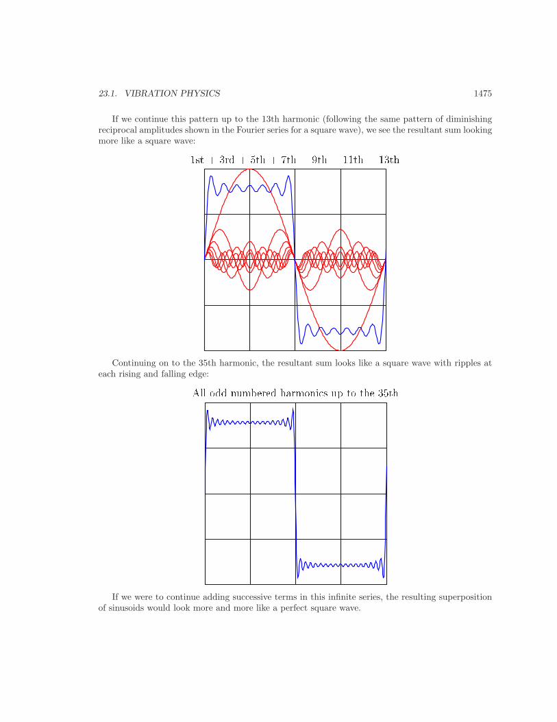
If we continue this pattern up to the 13th harmonic (following the same pattern of diminishingreciprocal amplitudes shown in the Fourier series for a square wave), we see the resultant sum lookingmore like a square wave:1st + 3rd + 5th + 7th + 9th + 11th + 13th

Continuing on to the 35th harmonic, the resultant sum looks like a square wave with ripples ateach rising and falling edge:All odd-numbered harmoni s up to the 35th

If we were to continue adding successive terms in this infinite series, the resulting superpositionof sinusoids would look more and more like a perfect square wave.


The only real question in any practical application is, “What are the A, B, and ω coefficientvalues necessary to describe a particular non-periodic waveform using a Fourier series?” Fourier’stheorem tells us we should be able to represent any periodic waveform – no matter what its shape– by summing together a particular series of sinusoids of just the right amplitudes and frequencies,but actually determining those amplitudes and frequencies is a another matter entirely. Fortunately,modern computational techniques such as the Fast Fourier Transform (or FFT ) algorithm makeit very easy to sample any periodic waveform and have a digital computer calculate the relativeamplitudes and frequencies of its constituent harmonics. The result of a FFT analysis is a summaryof the amplitudes, frequencies, and (in some cases) the phase angle of each harmonic.

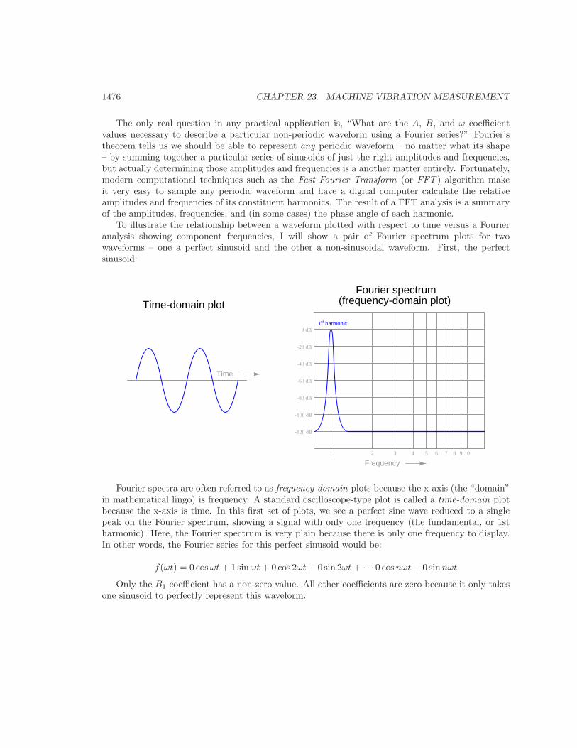
To illustrate the relationship between a waveform plotted with respect to time versus a Fourieranalysis showing component frequencies, I will show a pair of Fourier spectrum plots for twowaveforms – one a perfect sinusoid and the other a non-sinusoidal waveform. First, the perfectsinusoid:

0 dB

-20 dB

-40 dB

-60 dB

-80 dB

-100 dB

-120 dB

1 2 3 4 5 6 7 8 9 10

Time-domain plot

Frequency

Time

Fourier spectrum(frequency-domain plot)

1st harmonic

Fourier spectra are often referred to as frequency-domain plots because the x-axis (the “domain”in mathematical lingo) is frequency. A standard oscilloscope-type plot is called a time-domain plotbecause the x-axis is time. In this first set of plots, we see a perfect sine wave reduced to a singlepeak on the Fourier spectrum, showing a signal with only one frequency (the fundamental, or 1stharmonic). Here, the Fourier spectrum is very plain because there is only one frequency to display.In other words, the Fourier series for this perfect sinusoid would be:

f(ωt) = 0 cos ωt + 1 sin ωt + 0 cos 2ωt + 0 sin 2ωt + · · · 0 cos nωt + 0 sin nωt

Only the B1 coefficient has a non-zero value. All other coefficients are zero because it only takesone sinusoid to perfectly represent this waveform.


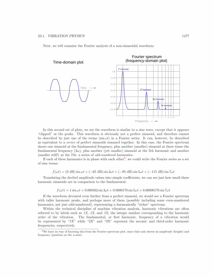
Next, we will examine the Fourier analysis of a non-sinusoidal waveform:

0 dB

-20 dB

-40 dB

-60 dB

-80 dB

-100 dB

-120 dB

1 2 3 4 5 6 7 8 9 10

Time-domain plot

Frequency

Time

Fourier spectrum(frequency-domain plot)

1st harmonic

3rd harmonic

5th harmonic

7th harmonic

In this second set of plots, we see the waveform is similar to a sine wave, except that it appears“clipped” at the peaks. This waveform is obviously not a perfect sinusoid, and therefore cannotbe described by just one of the terms (sin ωt) in a Fourier series. It can, however, be describedas equivalent to a series of perfect sinusoids summed together. In this case, the Fourier spectrumshows one sinusoid at the fundamental frequency, plus another (smaller) sinusoid at three times thefundamental frequency (3ω), plus another (yet smaller) sinusoid at the 5th harmonic and another(smaller still!) at the 7th: a series of odd-numbered harmonics.

If each of these harmonics is in phase with each other5, we could write the Fourier series as a setof sine terms:

f(ωt) = (0 dB) sin ωt + (−65 dB) sin 3ωt + (−95 dB) sin 5ωt + (−115 dB) sin 7ωt

Translating the decibel amplitude values into simple coefficients, we can see just how small theseharmonic sinusoids are in comparison to the fundamental:

f(ωt) = 1 sin ωt + 0.000562 sin 3ωt + 0.0000178 sin 5ωt + 0.00000178 sin 7ωt

If the waveform deviated even further from a perfect sinusoid, we would see a Fourier spectrumwith taller harmonic peaks, and perhaps more of them (possibly including some even-numberedharmonics, not just odd-numbered), representing a harmonically “richer” spectrum.

Within the technical discipline of machine vibration analysis, harmonic vibrations are oftenreferred to by labels such as 1X, 2X, and 3X, the integer number corresponding to the harmonicorder of the vibration. The fundamental, or first harmonic, frequency of a vibration wouldbe represented by “1X” while “2X” and “3X” represent the second- and third-order harmonicfrequencies, respectively.

5We have no way of knowing this from the Fourier spectrum plot, since that only shows us amplitude (height) andfrequency (position on the x-axis).


On a practical note, the Fourier analysis of a machine’s vibration waveform holds clues to thesuccessful balancing of that machine. A first-harmonic vibration may be countered by placing anoff-center mass on the rotating element 180 degrees out of phase with the offending sinusoid. Giventhe proper phase (180o – exactly opposed) and magnitude, any harmonic may be counterbalancedby an off-center mass rotating at the same frequency. In other words, we may cancel any particularharmonic vibration with an equal and opposite harmonic vibration.

If you examine the “crankshaft” of a piston engine, for example, you will notice counterweightswith blind holes drilled in specific locations for balancing. These precisely-trimmed counterweightscompensate for first-harmonic (fundamental) frequency vibrations resulting from the up-and-down oscillations of the pistons within the cylinders. However, in some engine designs such asinline 4-cylinder arrangements, there are significant harmonic vibrations of greater order than thefundamental, which cannot be counterbalanced by any amount of weight, in any location, on therotating crankshaft. The reciprocating motion of the pistons and connecting rods produce periodicvibrations that are non-sinusoidal, and these vibrations (like all periodic, non-sinusoidal waveforms)are equivalent to a series of harmonically-related sinusoidal vibrations.

Any weight attached to the crankshaft will produce a first-order (fundamental) sinusoidalvibration, and that is all. In order to counteract harmonic vibrations of higher order, the enginerequires counterbalance shafts spinning at speeds corresponding to those higher orders. This is whymany high-performance inline 4-cylinder engines employ counterbalance shafts spinning at twice thecrankshaft speed: to counteract the second-harmonic vibrations created by the reciprocating parts.If an engine designer were so inclined, he or she could include several counterbalance shafts, eachone spinning at a different multiple of the crankshaft speed, to counteract as many harmonics aspossible. At some point, however, the inclusion of all these shafts and the gearing necessary toensure their precise speeds and phase shifts would interfere with the more basic design features ofthe engine, which is why you do not typically see an engine with multiple counterbalance shafts.

The harmonic content of a machine’s vibration signal in and of itself tells us little about thehealth or balance of that machine. It may be perfectly normal for a machine to have a very “rich”harmonic signature due to convoluted motions of its parts6. However, Fourier analysis provides asimple way to quantify complex vibrations and to archive them for future reference. For example, wemight gather vibration data on a new machine immediately after installation (including its Fourierspectra on all vibration measurement points) and store this data for safe keeping in the maintenancearchives. Later, if and when we suspect a vibration-related problem with this machine, we maygather new vibration data and compare it against the original “signature” spectra to see if anythingsubstantial has changed. Changes in harmonic amplitudes and/or the appearance of new harmonicsmay point to specific problems inside the machine. Expert knowledge is usually required to interpretthe spectral changes and discern what those specific problem(s) might be, but at least this techniquedoes have diagnostic value in the right hands.

6Machines with reciprocating components, such as pistons, cam followers, poppet valves, and such are notoriousfor generating vibration signatures which are anything but sinusoidal even under normal operating circumstances!

23.2. VIBRATION SENSORS 1479

23.2 Vibration sensors

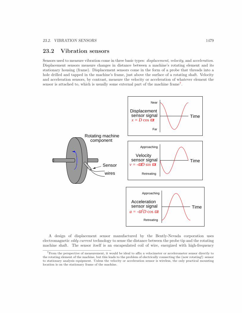
Sensors used to measure vibration come in three basic types: displacement, velocity, and acceleration.Displacement sensors measure changes in distance between a machine’s rotating element and itsstationary housing (frame). Displacement sensors come in the form of a probe that threads into ahole drilled and tapped in the machine’s frame, just above the surface of a rotating shaft. Velocityand acceleration sensors, by contrast, measure the velocity or acceleration of whatever element thesensor is attached to, which is usually some external part of the machine frame7.

wires

TimeDisplacement

Near

Far

TimeVelocity

Approaching

Retreating

x = D cos ωt

v = -ωD sin ωt

Time

Approaching

Retreating

Acceleration

a = -ω2D cos ωt

Sensor

sensor signal

sensor signal

sensor signal

Rotating machinecomponent

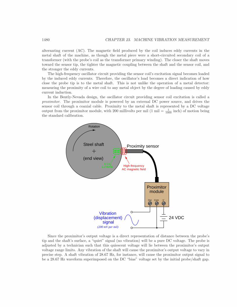
A design of displacement sensor manufactured by the Bently-Nevada corporation useselectromagnetic eddy current technology to sense the distance between the probe tip and the rotatingmachine shaft. The sensor itself is an encapsulated coil of wire, energized with high-frequency

7From the perspective of measurement, it would be ideal to affix a velocimeter or accelerometer sensor directly tothe rotating element of the machine, but this leads to the problem of electrically connecting the (now rotating!) sensorto stationary analysis equipment. Unless the velocity or acceleration sensor is wireless, the only practical mountinglocation is on the stationary frame of the machine.


alternating current (AC). The magnetic field produced by the coil induces eddy currents in themetal shaft of the machine, as though the metal piece were a short-circuited secondary coil of atransformer (with the probe’s coil as the transformer primary winding). The closer the shaft movestoward the sensor tip, the tighter the magnetic coupling between the shaft and the sensor coil, andthe stronger the eddy currents.

The high-frequency oscillator circuit providing the sensor coil’s excitation signal becomes loadedby the induced eddy currents. Therefore, the oscillator’s load becomes a direct indication of howclose the probe tip is to the metal shaft. This is not unlike the operation of a metal detector:measuring the proximity of a wire coil to any metal object by the degree of loading caused by eddycurrent induction.

In the Bently-Nevada design, the oscillator circuit providing sensor coil excitation is called aproximitor. The proximitor module is powered by an external DC power source, and drives thesensor coil through a coaxial cable. Proximity to the metal shaft is represented by a DC voltageoutput from the proximitor module, with 200 millivolts per mil (1 mil = 1

1000 inch) of motion beingthe standard calibration.

Steel shaft

(end view)

Proximity sensor

Proximitor

24 VDCsignal

High-frequencyAC magnetic field

Rotation

Eddycurrents

module

ComOut -V

Vibration(displacement)

(200 mV per mil)

Since the proximitor’s output voltage is a direct representation of distance between the probe’stip and the shaft’s surface, a “quiet” signal (no vibration) will be a pure DC voltage. The probe isadjusted by a technician such that this quiescent voltage will lie between the proximitor’s outputvoltage range limits. Any vibration of the shaft will cause the proximitor’s output voltage to vary inprecise step. A shaft vibration of 28.67 Hz, for instance, will cause the proximitor output signal tobe a 28.67 Hz waveform superimposed on the DC “bias” voltage set by the initial probe/shaft gap.

23.2. VIBRATION SENSORS 1481

An oscilloscope connected to this output signal will show a direct representation of shaft vibration,as measured in the axis of the probe. In fact, any electronic test equipment capable of analyzingthe voltage signal output by the proximitor may be used to analyze the machine’s vibration:oscilloscopes, spectrum analyzers, peak-indicating voltmeters, RMS-indicating voltmeters, etc.

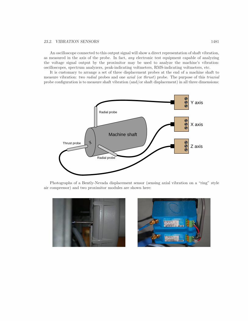
It is customary to arrange a set of three displacement probes at the end of a machine shaft tomeasure vibration: two radial probes and one axial (or thrust) probe. The purpose of this triaxialprobe configuration is to measure shaft vibration (and/or shaft displacement) in all three dimensions:

Machine shaft

Y axis

X axis

Z axis

Radial probe

Radial probe

Thrust probe

Photographs of a Bently-Nevada displacement sensor (sensing axial vibration on a “ring” styleair compressor) and two proximitor modules are shown here:


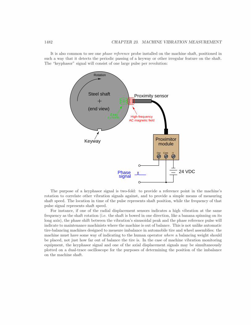
It is also common to see one phase reference probe installed on the machine shaft, positioned insuch a way that it detects the periodic passing of a keyway or other irregular feature on the shaft.The “keyphasor” signal will consist of one large pulse per revolution:

Steel shaft

(end view)

Proximity sensor

Proximitor

24 VDCsignal

High-frequencyAC magnetic field

Rotation

Eddycurrents

moduleKeyway

Phase

ComOut -V

The purpose of a keyphasor signal is two-fold: to provide a reference point in the machine’srotation to correlate other vibration signals against, and to provide a simple means of measuringshaft speed. The location in time of the pulse represents shaft position, while the frequency of thatpulse signal represents shaft speed.

For instance, if one of the radial displacement sensors indicates a high vibration at the samefrequency as the shaft rotation (i.e. the shaft is bowed in one direction, like a banana spinning on itslong axis), the phase shift between the vibration’s sinusoidal peak and the phase reference pulse willindicate to maintenance machinists where the machine is out of balance. This is not unlike automatictire-balancing machines designed to measure imbalance in automobile tire and wheel assemblies: themachine must have some way of indicating to the human operator where a balancing weight shouldbe placed, not just how far out of balance the tire is. In the case of machine vibration monitoringequipment, the keyphasor signal and one of the axial displacement signals may be simultaneouslyplotted on a dual-trace oscilloscope for the purposes of determining the position of the imbalanceon the machine shaft.

23.3. MONITORING HARDWARE 1483

23.3 Monitoring hardware

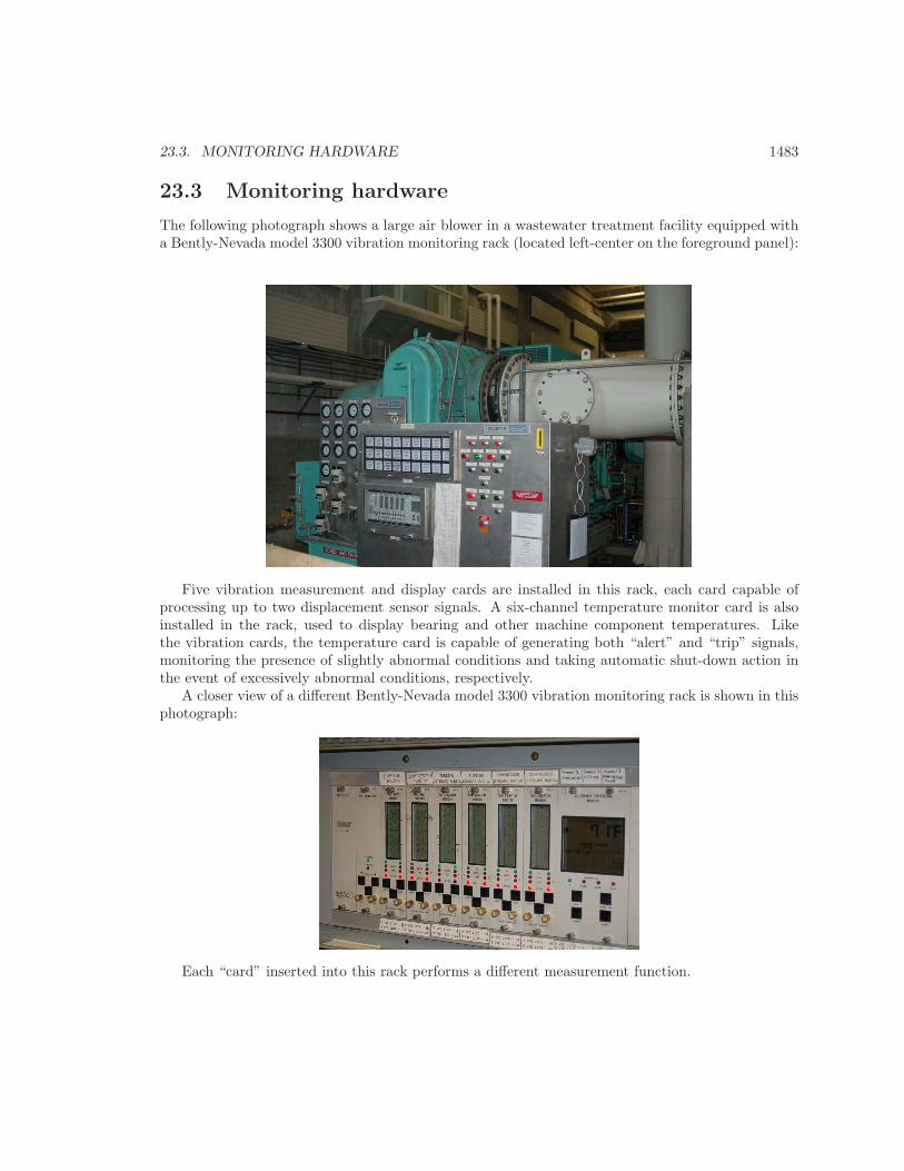
The following photograph shows a large air blower in a wastewater treatment facility equipped witha Bently-Nevada model 3300 vibration monitoring rack (located left-center on the foreground panel):

Five vibration measurement and display cards are installed in this rack, each card capable ofprocessing up to two displacement sensor signals. A six-channel temperature monitor card is alsoinstalled in the rack, used to display bearing and other machine component temperatures. Likethe vibration cards, the temperature card is capable of generating both “alert” and “trip” signals,monitoring the presence of slightly abnormal conditions and taking automatic shut-down action inthe event of excessively abnormal conditions, respectively.

A closer view of a different Bently-Nevada model 3300 vibration monitoring rack is shown in thisphotograph:

Each “card” inserted into this rack performs a different measurement function.


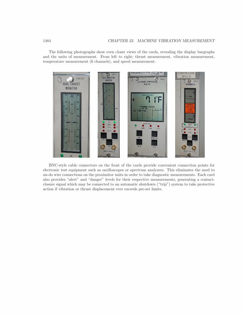
The following photographs show even closer views of the cards, revealing the display bargraphsand the units of measurement. From left to right; thrust measurement, vibration measurement,temperature measurement (6 channels), and speed measurement:

BNC-style cable connectors on the front of the cards provide convenient connection points forelectronic test equipment such as oscilloscopes or spectrum analyzers. This eliminates the need toun-do wire connections on the proximitor units in order to take diagnostic measurements. Each cardalso provides “alert” and “danger” levels for their respective measurements, generating a contact-closure signal which may be connected to an automatic shutdown (“trip”) system to take protectiveaction if vibration or thrust displacement ever exceeds pre-set limits.

23.3. MONITORING HARDWARE 1485

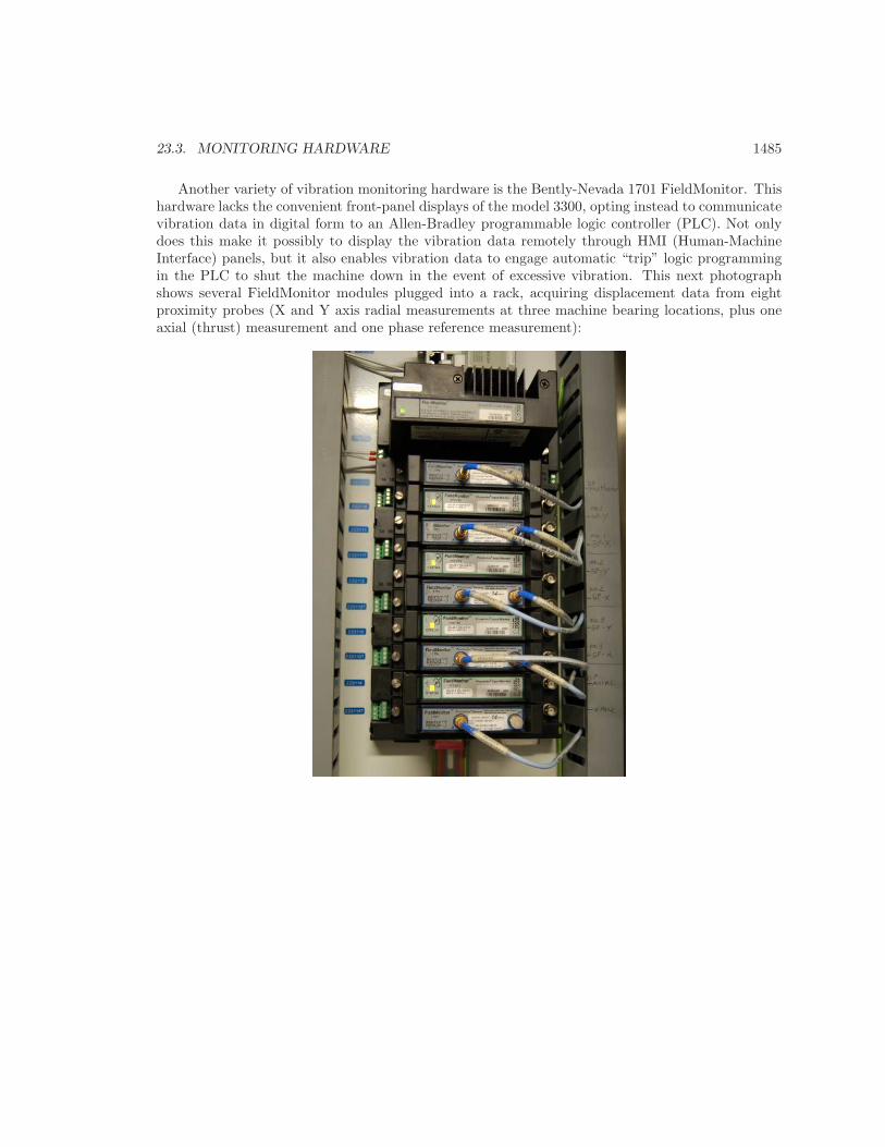
Another variety of vibration monitoring hardware is the Bently-Nevada 1701 FieldMonitor. Thishardware lacks the convenient front-panel displays of the model 3300, opting instead to communicatevibration data in digital form to an Allen-Bradley programmable logic controller (PLC). Not onlydoes this make it possibly to display the vibration data remotely through HMI (Human-MachineInterface) panels, but it also enables vibration data to engage automatic “trip” logic programmingin the PLC to shut the machine down in the event of excessive vibration. This next photographshows several FieldMonitor modules plugged into a rack, acquiring displacement data from eightproximity probes (X and Y axis radial measurements at three machine bearing locations, plus oneaxial (thrust) measurement and one phase reference measurement):


23.4 Mechanical vibration switches

A much simpler alternative to continuous vibration sensors (displacement or acceleration) andmonitoring equipment suitable for less critical applications is a simple mechanical switch actuated bya machine’s vibration. These switches cannot, of course, quantitatively analyze machine vibrations,but they do serve as qualitative indicators of gross vibration.

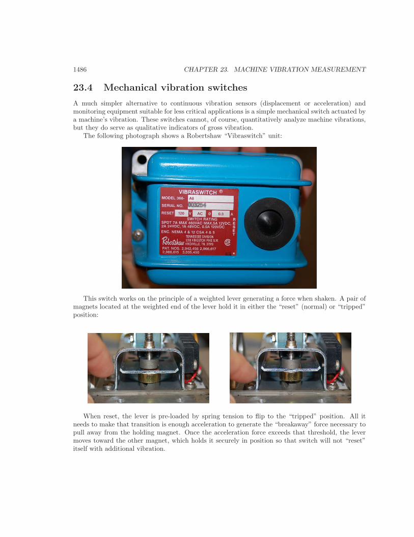
The following photograph shows a Robertshaw “Vibraswitch” unit:

This switch works on the principle of a weighted lever generating a force when shaken. A pair ofmagnets located at the weighted end of the lever hold it in either the “reset” (normal) or “tripped”position:

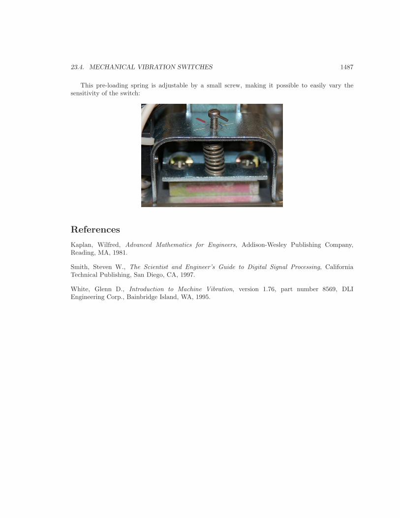
When reset, the lever is pre-loaded by spring tension to flip to the “tripped” position. All itneeds to make that transition is enough acceleration to generate the “breakaway” force necessary topull away from the holding magnet. Once the acceleration force exceeds that threshold, the levermoves toward the other magnet, which holds it securely in position so that switch will not “reset”itself with additional vibration.

23.4. MECHANICAL VIBRATION SWITCHES 1487

This pre-loading spring is adjustable by a small screw, making it possible to easily vary thesensitivity of the switch:

References

Kaplan, Wilfred, Advanced Mathematics for Engineers, Addison-Wesley Publishing Company,Reading, MA, 1981.

Smith, Steven W., The Scientist and Engineer’s Guide to Digital Signal Processing, CaliforniaTechnical Publishing, San Diego, CA, 1997.

White, Glenn D., Introduction to Machine Vibration, version 1.76, part number 8569, DLIEngineering Corp., Bainbridge Island, WA, 1995.

machine vibration basic

Documents