ABSTRACT PINE, WILLIAM EARL, III. Population Ecology of Introduced Flathead Catfish. (Under

the direction of Dr. Thomas J. Kwak and Dr. James A. Rice.)

Invasive aquatic species are becoming increasingly problematic for aquatic ecologists

and resource managers, as the ecological and economic impacts of introductions become

better known. The flathead catfish Pylodictis olivaris is a large piscivorous fish native to

most of the interior basin of the United States. Via legal and illegal introductions, they have

been introduced into at least 13 U.S. states and one Canadian province primarily along the

Atlantic slope. I used a variety of capture-recapture models to estimate flathead catfish

population parameters in three North Carolina coastal plain rivers (Contentnea Creek,

Northeast Cape Fear River, and Lumber River). My estimates using a Jolly-Seber model

were hindered by low capture probabilities and high temporary emigration. Reasonable

estimates were possible using a robust-design framework to estimate population size and

temporary emigration with supplemental information from a radio-telemetry study to

examine model assumptions. Population size estimates using a robust design model

including temporary emigration ranged from 4 to 31 fish/km (>125-mm total length, TL) of

sampling reach. Additional analyses showed high rates of temporary emigration (>90%),

independently supported by radio-telemetry results. I also examined flathead catfish diet in

these rivers and found that flathead catfish fed on a wide variety of freshwater fish and

invertebrates, anadromous fish, and occasionally estuarine fish and invertebrates. Fish or

crayfish comprised more than 50% of the stomach contents by percent occurrence, percent-

by-number, and percent-by-weight in all rivers and years. A significant difference in the diet

composition percent-by-number was found between Contentnea Creek and the Northeast

Cape Fear River. Significant differences were not detected between years within Contentnea

Creek but were found within the Northeast Cape Fear River. Feeding intensity (as measured

by stomach fullness) was highest in the Northeast Cape Fear River associated with a lower

mean size of feeding flathead catfish in this river than of those in Contentnea Creek or the

Lumber River. A significant correlation between diet item length and flathead catfish total

length was found for Contentnea Creek in 2001. This relationship was not significant in the

Northeast Cape Fear River in either year. Based on the diet composition data collected in

this study and those published on native and introduced flathead catfish populations, I am not

able to support or refute the hypothesis that flathead catfish are preferentially feeding on

specific species or families. However, the flathead catfish populations examined here are

well established, and the greatest impact from selective predation may have occurred

immediately following introduction. Based on my findings, flathead catfish could restructure

or suppress native fish communities in coastal rivers through direct predation because of their

primarily piscivorous food habits. To evaluate the potential ecosystem impact of this

invasive species on the native fish community, I developed an ecosystem simulation model

(including flathead catfish) based on empirical data collected for a North Carolina coastal

river. Model results suggest that flathead catfish suppress native fish community biomass by

5-50% through both predatory and competitive interactions. However, these reductions

could be mitigated through sustained exploitation of flathead catfish by recreational or

commercial fishers at levels equivalent to those for native flathead catfish populations (6-

25% annual exploitation). These findings demonstrate the potential for using directed

harvest of an invasive species to mitigate the negative impacts to native species.

POPULATION ECOLOGY OF INTRODUCED FLATHEAD CATFISH

by

WILLIAM E. PINE, III

A dissertation submitted to the Graduate Faculty of North Carolina State University

in partial fulfillment of the Requirements for the Degree of

Doctor of Philosophy

Department of Zoology

Raleigh

2003

APPROVED BY:

__________________________________ _________________________________ Dr. Thomas J. Kwak Dr. James A. Rice Co-chair of Advisory Committee Co-chair of Advisory Committee _____________________________ ____________________________ Dr. Joseph E. Hightower Dr. Kenneth H. Pollock

ii

BIOGRAPHY

I was born William (Bill) Earl Pine, III to Loye Zeanah Pine and William (Kip) Earl

Pine, Jr. on 20 August 1975, in Grove Hill, Alabama. My academic and career path is an

extension of childhood opportunities and experiences across the great state of Alabama. I

began my fisheries education at Auburn University in the fall of 1993. My experiences at

Auburn University were formative in shaping me into the person that I am now. An early

mentor, Dr. Bill Davies, helped me to secure a position working with Dr. Dennis DeVries, in

whose lab I remained during my four years at Auburn. It was through my work with the

outstanding members of this lab that I developed the professional skills and friendships that

have carried me through my Ph.D. Following graduation from Auburn in 1997, I began my

M.S. degree with Dr. Mike Allen at the University of Florida. Dr. Allen was both generous

in the learning and research opportunities he provided, and rigorous in his expectations of

my performance. I thrived in this work environment and consider Mike to be one of my best

professional and personal friends. Following graduation from the University of Florida in

the fall of 1999, I was recruited by a long-time friend, Dr. Rich Noble, for the Ph.D. program

in Zoology at North Carolina State University. I moved to Raleigh in the summer of 2000

and enrolled in the Zoology Department under the supervision of Drs. Tom Kwak and Jim

Rice. My research on introduced riverine populations of flathead catfish has been the most

challenging fisheries project with which I have been involved. I defended my dissertation in

the fall of 2003, and I am now looking forward to the next learning opportunity.

iii

ACKNOWLEDGMENTS

A Federal Aid in Sport Fish Restoration grant (F-68) through the North Carolina

Wildlife Resources Commission, Division of Inland Fisheries supported this research. I

would like to thank my advisors Dr. Tom Kwak and Dr. Jim Rice for this opportunity and

their support throughout my research and academic program. I would also like to thank my

committee members Dr. Joe Hightower and Dr. Ken Pollock for their active participation

and insight into this project. Special thanks also to Dr. Rich Noble for his mentorship during

this project and throughout my career.

This project was a massive undertaking requiring careful planning and a large field

effort. The name “Team Flathead” developed early and remains appropriate– this project

was truly a team effort. I thank Scott Waters, NCSU Research Associate, for his efforts and

participation in every aspect of the project. Drew Dutterer and Ed Malindzak provided good

attitudes and outstanding technical support throughout long and difficult field days. Wendy

Moore, NC Coop Unit Program Assistant provided tremendous logistical support. Christian

Waters, Keith Ashley, Tom Rachels, Kent Nelson, Pete Kornegay, and Scott Van Horn from

the NCWRC readily provided field assistance and technical insight throughout this project.

I owe tremendous thanks to my family, particularly my wife Julie. She has

graciously and lovingly supported my learning efforts in every way asked. My parents

recognized my early interest in science and have unwaveringly supported me. The cost of

this support cannot be measured and simple thanks is not enough– I can assure you that I

will do the same for my children in your honor. My brother David and sister Rebekah have

always provided loving support and inspiration to me. I have a large extended family of

iv

Aunts, Grandparents, and in-laws to which I am grateful. Knowing that your family

supports you is a tremendous help in the often solo pursuit of knowledge.

v

TABLE OF CONTENTS

Page

LIST OF TABLES vii LIST OF FIGURES ix CHAPTER 1. INTRODUCTION 1 Introduction and Justification 2 CHAPTER 2. A REVIEW OF TAGGING METHODS FOR ESTIMATING FISH POPULATION SIZE AND COMPONENTS OF MORTALITY Abstract 5 Introduction 6 Capture-recapture Models 10 Closed Models 11 Open Models 17 Robust Design 20

Tag Return Models 22 Telemetry Methods 25 Combined Tagging-telemetry Models 28

Conclusions 29 References 31

CHAPTER 3. ESTIMATING POPULATION SIZE OF AN INVASIVE CATFISH IN COASTAL RIVERS Abstract 44 Introduction 45 Methods 47 Results 53 Jolly-Seber 54 Robust Design 57 Discussion 60 Recommendations and Conclusions 69 References 72 CHAPTER 4. FOOD HABITS OF INTRODUCED FLATHEAD CATFISH Abstract 92 Introduction 93 Methods 95

vi

Results 97 Contentnea Creek 98 Northeast Cape Fear River 99 Lumber River 99

Discussion 101 Future Work 109 Conclusions and Management Recommendations 110

References 112 CHAPTER 5. MODELING THE EFFECTS OF AN INTRODUCED APEX PREDATOR ON A COASTAL RIVERINE FISH COMMUNITY Abstract 129 Introduction 129 Methods 133 Results 138 Invasion Simulation 138 Eradication Simulation 139 Resiliency Simulation 140 Discussion 140 Management Implications 145 References 149 Appendices 162 CHAPTER 6. SYNTHESIS AND DIRECTION OF FUTURE RESEARCH Synthesis 169 Future Research 173 References 175

vii

LIST OF TABLES

Page

Table 2.1 Product name, description, and World Wide Web address for various software packages to assist with analyzing data from tagging studies. 37

Table 2.2 Model, type of mark required (batch or individual), source of fish used in study (research collection or fishery dependent), typical study duration, reporting rate requirement, key parameters, additional information generated, and principal software for estimating population size and mortality components from tagging models discussed in this review. 38

Table 3.1 Name and description of each model fit to capture-recapture data

collected in each river during either 2001, 2002, or both. 77 Table 3.2 Year, river, sample reach, number of samples, catch-per-unit-effort

(CPUE), and standard error (SE) of flathead catfish catch for each river during 2001 and 2002. 78

Table 3.3 Open population model results for each year, river, and reach where

an open model was able to fit the data. 79 Table 3.4 River, reach, model name, AICc value, delta AICc, AICc weight, and

number of model parameters for each robust design model fit to the data. 80

Table 3.5 River name, sample reach, model name survival rate (Φ + SE,

emigration rate (G" + SE) between primary periods 1 and 2, emigration rate (G" + SE) between primary periods 2 and 3, immigration rate (G' + SE), capture probability ( $p+ SE), recapture probability ( $c + SE, and population size (N + SE) for each primary period in 2002. 81

Table 3.6 River, reach, model name, AICc value, delta AICc, AICc weight,

and number of model parameters for random temporary emigration robust design models to data collected in 2002. Models were fit with and without empirical estimates of capture and recapture probability from radio-tagged fish. Bold indicates best-fit model with lowest AICc value and highest AICc weight. 83

viii

Table 3.7 River name, sample reach, model name survival rate (Φ + SE), emigration rate (G" + SE ) between primary periods 1 and 2, emigration rate (G" + SE) between primary periods 2 and 3, capture probability ( $p+ SE), recapture probability ( $c+ SE), and population size per-km (N+ SE) for each primary period in 2002 using the random temporary emigration model with and without capture probability information from radio tags. 84

Table 3.8 Flathead catfish population biomass and density with associated standard

error and approximate 95% confidence intervals (±2SE) estimated for each river, reach, and month. 86

Table 4.1 Family and common names of typical representatives from each family

found in flathead catfish stomachs in Contentena Creek, Northeast Cape Fear River, and the Lumber River, 2001-2002. 115

Table 4.2 Year, river, prey item, frequency of occurrence, and rank (in ascending

order) of stomach items. 116 Table 4.3 Year, river, prey item, mean percent frequency of that item, standard

error and rank (ascending order) of stomach items found in flathead catfish. 118

Table 4.4 Year, river, prey family, total weight of family in stomach contents,

percentage of the total weight for all stomach contents, and rank (ascending order) of stomach items found in flathead catfish. 120

Table 4.5 Year, river, prey family, number of identifiable prey from that family,

mean weight identifiable items, standard error of the mean, and rank (ascending order) of stomach items found in flathead catfish. 122

Table 4.6 Sample year, sample month, river, sample size, TL (mm) ± SE,

weight (g) ± SE, and stomach fullness ± SE of flathead catfish with stomach contents. 124

Table 5.1 Species composition of each functional group included in the Ecopath

model. 153

ix

LIST OF FIGURES Page Figure 2.1 Diagram demonstrating assumptions about capture probabilities

for each type of capture-recapture model discussed in this chapter. 39 Figure 2.2 Schematic drawing of the robust-design model demonstrating open and

closed periods as well as estimable parameters at each period. 40 Figure 3.1 Seasonal CPUE (number of fish / hour) for reach 1 in Contentnea

Creek during preliminary sampling in 2000 and Jolly-Seber open population sampling in 2001. 87

Figure 3.2 Open population model estimates for reach 1 and reach 2 in Contentnea

Creek during 2001. 88 Figure 3.3 Estimated population size (+ SE) for each sample reach during each

primary period from Contentnea Creek during 2001 and 2002 using the best fit model (see text), a robust design model with random temporary emigration. 89

Figure 3.4 Estimated population (+ SE) size kilometer of sample reach during each

primary period from the Northeast Cape Fear River during 2002. 90

Figure 4.1 Correlation between diet item size (mm) and flathead catfish (FHC) total length (mm) for Contentnea Creek and the Northeast Cape Fear River in 2001 and 2002. 126

Figure 5.1 Simplified food web schematic demonstrating linkages among functional

groups in Contentnea Creek. 154 Figure 5.2 Simulated ecosystem response to flathead catfish introduction in a

coastal river. 155 Figure 5.3 Relative percent change in biomass of freshwater, estuarine, and

anadromous fish groups to changes in flathead catfish exploitation rates over a 20-year period. 156

Figure 5.4 Simulated ecosystem response to flathead catfish eradication through

intensive exploitation measured as relative percent change in biomass of freshwater, estuarine, and anadromous fish groups. 158

Figure 5.5 Simulated resiliency of flathead catfish of flathead catfish populations to

intensive exploitation. 160

x

Figure 5.6 Maintenance control simulation demonstrating the response of native fish groups to oscillating levels of flathead catfish exploitation. 161

1

CHAPTER 1

INTRODUCTION

2

Introduction and Justification

The introduction of non-native species is an ecologically significant, yet poorly

understood component of anthropogenic aquatic habitat alteration. The impact of non-native

species can be evaluated ecologically via functional or species changes within the introduced

ecosystem or economically by cost estimates to mitigate ecosystem changes following

species introduction. The purpose of this dissertation is to evaluate the ecological

interactions between native fish communities and a non-native, piscivorous flathead catfish

Pylodictis olivaris, in three coastal North Carolina rivers.

Flathead catfish are large predatory fish native to most river systems within the

interior basin of the United States and now introduced along much of the mid-Atlantic slope

and portions of the Pacific slope. Flathead catfish have currently established reproducing

populations in at least 13 US States and one Canadian province (Jackson 1999). Flathead

catfish have frequently been introduced as a recreational sportfish species because of their

potential for large size, fighting ability when hooked, and palatable flesh. No ecologically

similar native species exist within the introduced range. Following the introduction of

flathead catfish, there have been corollary declines in a wide variety of native fish species

including native catfishes and sunfishes. This has led to widespread concern that the

establishment of flathead catfish may come at the expense of native fish diversity and

inherent biological stability.

To study these interactions between native fish communities and flathead catfish, I

estimated population size and sampled stomach contents of flathead catfish and determined

native fish community composition and abundance in three coastal North Carolina rivers. I

3

then linked this information for flathead catfish and native fish groups in a mass balance

(Ecopath) model to examine energy transfer linkages between the native fish community and

flathead catfish. Finally, I used the mass balance model to simulate changes in ecosystem

structure following intensive harvest of flathead catfish at various exploitation rates. These

findings were then compiled and presented as a potential impact scenario following flathead

introduction and compared to the original flathead catfish introduction in North Carolina.

Also, several potential management scenarios related to flathead catfish harvest as a tool to

assist with native fish community restoration were evaluated.

This dissertation is presented as five manuscripts. Chapter Two is a review of

capture-recapture methods for estimating population size. This chapter has been accepted

for publication in Fisheries and is written in first-person plural tense to reflect the joint

authorship among myself, Ken Pollock, Joe Hightower, Tom Kwak, and Jim Rice. Other

chapters are written in first-person singular tense. Chapter Three is a capture-recapture study

to estimate flathead catfish population size in each study river. Chapter Four is an analysis

of the flathead catfish stomach content data. Chapter Five is a series of models which

synthesize each of the above components and evaluate ecosystem response to flathead

catfish introduction and harvest. Chapter Six discusses how these findings fit a set of

empirically derived rules describing other invasive aquatic species and provides

recommendations for future research related to introduced flathead catfish ecology.

4

CHAPTER 2

A REVIEW OF TAGGING METHODS FOR ESTIMATING FISH POPULATION SIZE AND COMPONENTS OF MORTALITY

5

Abstract

Techniques to improve estimation of animal population size and mortality from

tagging studies have received substantial attention from terrestrial biologists and statisticians

during the last 20 years. However, these techniques have received little notice from fisheries

biologists, despite the widespread applicability to fisheries research, the wide variety of tag

types used in fisheries research (from traditional fin clips to telemetry tags), and the

development of new computer software to assist with analyses. We present a brief review of

population models based on recaptures, returns, or telemetry relocations of tagged fish that

can be used to estimate population size, total mortality, and components of mortality (i.e.,

fishing and natural) that are frequently of interest to fisheries biologists. Recommended

strategies include (1) use closed population models (e.g., Lincoln-Petersen) to estimate

population size for short term studies where closure assumption can be met, (2) use the

robust design to estimate population size for studies of longer duration, (3) use high-reward

tags in conjunction with other methods of estimating reporting rate in tag-return studies, (4)

combine a subset of telemetry tagged fish with either a high-reward tagging program or a

traditional capture-recapture study to improve mortality estimates and understanding of

mortality components, and (5) use pilot studies and simulation analyses to assess precision of

estimated parameters to evaluate study feasibility. Incorporation of these improved

techniques could lead to greater accuracy and precision of parameter estimates from tagging

studies and thus to improved understanding and management of fish populations.

6

Introduction

Effective fisheries management often requires reliable information on population size,

survival, and mortality. For example, the population size of imperiled fish species is often a

critical factor in determining its protected status, and recovery plans often focus on ways to

increase species abundance by understanding mortality components and reducing mortality

rates (Pine et al. 2001). Management actions such as the evaluation of marine protection

areas also frequently use indices of animal abundance to assess the effectiveness of

restrictions on fishing mortality (Russ and Alcala 1996). Fish stocks with commercial and

recreational value are usually managed with a goal of maintaining sustainable harvests

through regulation of fishing mortality (Hilborn and Walters 1992).

Capture-recapture methods with tagged animals are a primary means of estimating

the abundance and survival of animal populations. These methods have received

considerable attention over the last century from wildlife biologists and statisticians

interested in developing applied statistical models to estimate animal abundance (Pollock

1991; Williams et al. 2002). Tag-return methods are also a primary means of estimating a

population’s total mortality rate, and in some fisheries settings, the natural and fishing

components of mortality (Brownie et al. 1985; Hoenig et al. 1998a; Pollock et al. 2001a).

Such tag return models are basically special extensions of capture-recapture models used to

estimate population size, survival rates, and recruitment (i.e., “Jolly-Seber” models, Seber

1982). The key difference is, for a capture-recapture model, the biologist conducts the

sampling at specific points in time to recapture tagged fish alive. For application of a tag-

7

return model, returns of harvested fish come from one or more fisheries over an extended

period of time (e.g., fishing season).

It is our observation that fisheries biologists have been less aggressive in adopting

these models for estimating population size, survival rates, and mortality rates, relative to our

wildlife counterparts. This may be due to unfamiliarity with the methods or software as well

as practical concerns. We also have observed that tagging studies to estimate population size

and survival rates (e.g., Jolly-Seber) are frequently considered separately from tagging

studies used to estimate mortality rates (e.g., Brownie models). Information from both study

types is useful to fisheries managers, and the purpose of this article is to review tagging

methods for estimating population size and mortality components for fisheries applications.

Our review is intended to assist fisheries biologists in designing tagging studies by

summarizing the underlying assumptions and basic models available within the framework of

available specialized software (Box 1, Tables 1 and 2). Our hope is that this review will

encourage fisheries biologists to utilize these techniques in their research efforts.

Capture-recapture versus Catch-per-unit-effort

Catch-per-unit-effort (CPUE) data are often used as a relative index of population

size. However, this approach assumes that catchability or probability of capture is consistent

over time. The relationship between catch rate and actual abundance is not generally

considered, and it is unlikely that capture probability will be constant over time and under

varying sampling conditions (Williams et al. 2002). That relationship is important, because

fish sampling techniques rarely collect all animals present in an area and fish behaviors (e.g.,

schooling) may concentrate fish such that catches remain high, even if populations are

8

declining (Hilborn and Walters 1992). Capture-recapture models provide direct estimates of

both population size and the probability of capturing an individual while CPUE only

demonstrates trends in catches which may (or may not) be related to population abundance

(Williams et al. 2002). In general, if the primary study objective is to detect large (e.g.,

>50%) changes in population abundance, then CPUE data may be adequate. In situations

where more precise information on population size and trends, or information on mortality

and its components are of interest, then a tagging study is likely the best approach.

The two approaches can be compared by considering the common situation of

sampling largemouth bass (Micropterus salmoides) in reservoirs with shoreline electrofishing

transects. Due to gear avoidance or sampling difficulties related to physical structure, it is

unlikely that every largemouth bass along the shoreline is collected. Instead, we can

conceptualize a model where each fish will have a capture probability ( pi ), which can then

be used to estimate the number of largemouth bass in the transect ( $Ni ) from the number of

fish collected in the sample (Ci), where

$NCpi

i

i= . (1)

The capture probability, pi , is the probability of a fish being caught at that time (i) and

location with the gear employed. The use of estimates of capture probability ( $p ) to account

for individuals that are not collected in an area is critical to generating precise and accurate

estimates of population size.

Because capture probability is rarely constant, it is not possible to separate changes

in pi from changes in population size if CPUE is considered alone (Pollock et al. 2002;

9

Williams et al. 2002). Returning to our example, if an electrofishing sample collected along

the same transect six months later included only 10% of the number of fish caught in the

previous transect, is this because fewer fish are present along the shoreline, or has

the pi changed because of a change in water temperature, vegetative cover, or some other

environmental factor? Bayley and Austen (2002) demonstrated wide variation in the

catchability of lentic fishes across a range of fish species, fish size, and varying

environmental conditions. This is not surprising to field biologists who routinely notice

changes in catch rate with changes in environmental conditions (e.g., weather) or seasonal

patterns in recruitment and movement.

A key parameter in a capture-recapture study is the capture probability, which can be

defined as the probability that an individual animal is captured on a sampling occasion. In

practical terms, it can also be thought of as the fraction of the study population captured on

that occasion. It is generally estimated from the recapture of tagged individuals, and should

be as high as possible in order to obtain reliable estimates of population parameters.

Unfortunately, the literature and our own experiences in conducting these types of studies

have shown that capture probability is low in most fisheries studies, resulting in “sparse”

data. The typically low efficiency of fisheries sampling methods is illustrated by Bayley and

Austen (2002). They sampled known populations of various species in reservoirs and ponds

and reported empirical estimates of catchability (the fraction of fish collected in a single pass

in an electrofishing boat) that ranged from 2 –14%.

Tagging studies require that fish that are collected, tagged, and released be in good

condition and as likely to be captured (or harvested) as untagged fish in a future sample.

10

This compels biologists to use non-lethal collection techniques that may not be the most

efficient gears available. Collection restrictions placed on researchers by permitting agencies

may also limit the use of some techniques or sampling programs (e.g., placing limits on

gillnet soak time or electrofishing settings), particularly with imperiled species (Pine et al.

2001; Holliman et al. 2003). Because capture probability drives accuracy and precision of

parameter estimates, biologists should design their sampling programs to maximize capture

probability.

Capture-recapture models

One approach to estimating capture probability and population size is to use capture-

recapture (mark-recapture) methods. These methods have been intensively studied by

biostatisticians and applied widely to terrestrial wildlife populations (Lancia et al. 1994;

Williams et al. 2002). In these studies, fish are recaptured alive on multiple occasions, unlike

tag-return studies (described below) where there is only one “recapture” in the harvest - and

the fish is dead.

Capture-recapture models can be broadly defined as open or closed population

models, each with specific assumptions. Closed population models are “closed” to changes

in the population due to births, deaths, emigration, or immigration, whereas open models

allow for these changes. Both closed and open models estimate capture probability and

population size. In addition, open models are able to estimate apparent survival, recruitment,

and population change. Detailed explanations and examples of each are discussed below.

11

Closed Models

Models that assume equal catchability among individuals and sample dates, such as

Lincoln-Petersen and Schnabel models (Figure 1), have a long history of use in fisheries

applications (Ricker 1975). These models have strict assumptions that are frequently

violated to varying degrees, which results in biased population estimates. The basic Lincoln-

Petersen model is based on a sample of n1 animals caught, marked with individual (e.g., PIT

tag) or batch marks (e.g., fin clip), and released at time one. A second sample n2, is then

taken at time two and the number of marked animals m2 is noted. The equation for the

population estimate (Ricker 1975) is

$Nn nm

=1 2

2

. (2)

The rationale for this model is that the fraction of marked fish in the second sample (2

2

nm ),

should on average equal the fraction of the population that is marked (Nn1 ).

The widely used “Schnabel” model (Ricker 1975) is basically an extension of the

Lincoln-Petersen model that allows for more than two samples with a batch mark. The

assumptions for both models are that (1) the population is closed to additions (recruitment or

immigration) or deletions (deaths or emigration), (2) capture probability is equal among all

animals in each sample, and (3) marks are not lost or overlooked.

In capture-recapture studies lasting longer than a few days, the closed model

assumption of no additions or deletions occurring in the population may be unrealistic.

Although recruitment and mortality may be negligible or low for a species over a period of

12

time longer than a few days (perhaps even a season), movement into or out of the study area

often precludes the use of closed population models. A variety of studies have revealed

movement patterns in adult and juvenile fishes that would violate the closure assumption

(e.g., Cleary and Greenbank 1954; Skalski and Gilliam 2000; Hightower et al. 2001; Mitro

and Zale 2002).

Heterogeneity in capture probability may be an important source of bias if traditional

Lincoln-Petersen and Schnabel models are used. Heterogeneity can be related to differences

in fish size, sex, or social status (assumption 2, equal catchability). Many fisheries gears are

strongly size selective. For example, electrofishing is known to select for larger individuals

(Reynolds 1996), which likely leads to electrofishing samples containing disproportionate

numbers of large individuals relative to their actual abundance. Lincoln-Petersen and

Schnabel models do not account for such heterogeneity (which leads to strong negative bias

in population size). Estimates may be produced separately for important strata, (size, sex, or

status), to minimize heterogeneity within a stratum (Kwak 1992), but this approach results in

reduced sample sizes for each estimate and corresponding reduced precision. Program SPAS

can be used to analyze 2-sample capture-recapture data over several strata to account for

heterogeneity provided sufficient recaptures are collected within each strata (Table 1).

An additional source of variation in capture probability is “trap response” or

behavior, where capture probability depends on an animal’s previous capture experience. An

animal may be less or more likely to be caught in future samples because it has learned to

avoid, or is attracted to, a trap. For example, fish behavior was shown to be altered for at

least 24 h following electrofishing and marking (Mesa and Schreck 1989).

13

Tag loss is common in fisheries studies (Guy et al. 1996, violation of assumption 3)

and can result in very serious bias in $N . Tag loss can be estimated by double tagging some

individuals (Guy et al. 1996) and then adjusting the number of recaptures to account for this

loss. For this approach, tag loss must be assumed to be independent for the two tags. If

possible, tag type and location should be evaluated with a pilot study to ensure that tag

retention will be adequate, and provide the researcher with experience in tagging procedures.

The Lincoln-Petersen and Schnabel models are widely used in fisheries applications

because they are easily implemented, computationally simple, and most importantly,

individual fish do not have to be uniquely marked. Despite these advantages, we recommend

applying individual marks to obtain the complete capture history of each fish, so that the

degree of heterogeneity and trap response in capture probabilities may be assessed and

accounted for. Capture histories are often recorded as a series of 1s and 0s, where 1 indicates

an animal was caught in that sampling period, and 0 indicates the animal was not caught.

This method of recording capture histories of individual animals is the standard means of

entering data into capture-recapture software packages.

A suite of eight closed models has been developed to allow for variation in capture

probability related to physical, behavioral, and temporal attributes of the study species or

sampling design (Otis et al. 1978). These models are available in program CAPTURE, a

computer software program designed to assist with analyzing capture-recapture data

available at no cost through the World Wide Web as a stand alone program or accessed

through another free software program, MARK, discussed later (Table 1). Model Mo is the

simplest model for closed populations and does not allow for changes in capture probability

14

due to heterogeneity, behavior, or time (Pollock et al. 1990; Lancia et al. 1994). The

heterogeneity model (Mh) allows each animal to have a unique capture probability (due to

size, sex, etc.) but this capture probability must remain constant among all sampling periods

i. The trap response/behavior model Mb estimates an initial capture probability $p and

recapture probability ( $c ), which may differ from each other. Model Mt allows capture

probability to vary among sampling periods, but it must remain constant among individuals

for each period. This model is the same as the Schnabel model. Models Mtb, Mbh, Mth, and

Mtbh are combinations of the above, but require additional assumptions (for more detail see

Norris and Pollock 1995; Pledger 2000; Williams et al. 2002). Program CAPTURE is the

only specialized program available that can be used to fit each of these heterogeneity models

to capture histories from a capture-recapture study. Program CAPTURE also uses a model

selection approach based on a large number of goodness-of-fit tests to assist with choosing

the model that best fits the data. However, the model selection routine in CAPTURE does

not perform well with sparse data; thus, biologists should evaluate models closely in terms of

meeting assumptions to select the simplest model that best describes the data (Pollock et al.

1990; Williams et al. 2002).

The Schnabel model is simple in design and analysis and has been widely used in

fisheries applications (Ricker 1975; McInerny and Cross 1999; Kocovsky and Carline 2001).

Capture probability can vary among sampling periods with this model (analogous to model

Mt in CAPTURE). Although the Schnabel model is computationally simple (Table 2, no

need for computer analysis), we suggest using program CAPTURE for analyzing such data

because CAPTURE can fit and evaluate several models in addition to the Schnabel model.

15

For example, CAPTURE can compare the Mt (Schnabel) model, which does not allow for

heterogeneity, with the Mth model, which allows for varying capture probabilities among

individuals (heterogeneity) and among sampling occasions. The Mth model may be more

realistic because it accounts for heterogeneity, whereas the Mt is highly biased by unequal

capture probabilities (heterogeneity) within each time period (Lancia et al. 1994). We

consider heterogeneity in capture probability to be present in almost all fisheries applications

and suggest that the Schnabel model (Mt in CAPTURE) be used only if it is chosen by a

model selection procedure. However, in samples with extremely low capture probability

(<0.05), Mt (or the similar Chao Mt model also available in CAPTURE, Chao 1989) may be

the only model that CAPTURE is able to fit to the data for a population estimate (Mitro and

Zale 2002). In this case, estimates should be evaluated in terms of the severity of potential

assumption violations, particularly that for heterogeneity.

Removal Studies

Depletion or removal studies are widely used in fisheries applications and are

analogous to closed capture-recapture model Mb in CAPTURE (Ricker 1975; Otis et al.

1978). Mb allows for animals that have been captured previously to demonstrate a different

capture probability than those that have not been captured. This “trap response” is

mathematically analogous to a removal model because only initial captures of animals are

used in estimating population size (Pollock et al.1990). Model Mb assumes that the initial

capture probability is constant among animals. Model Mbh as applied to removal studies

relaxes that equal catchability assumption by allowing individual animals to have different

16

removal probabilities between animals but requires that the removal probability does not

change over time.

Similar to closed models, accurate population size estimates from removal studies

rely on minimally adequate capture probabilities and initial population size. White et al.

(1982) recommended capture probabilities of 0.2 and population sizes of 200 individuals

based on simulation studies for reliable population size estimates. There is also the question

of the number of samples. We recommend removal studies that incorporate four or more

samples to allow the possibility of accounting for heterogeneity among individuals.

CAPTURE’s maximum-likelihood estimation of N generates similar estimates to

those of the regression technique commonly used in removal studies (Lancia et al. 1994). A

disadvantage of the regression approach is the potential for violating assumptions required

for linear regression, such as homogenous variances among regressed points (Pollock 1991).

Because of this and other potential violations, the wider range of models available, and

model selection assistance provided in program CAPTURE, we re-emphasize the

recommendation of Lancia et al. (1994) and Pollock (1991) to use CAPTURE for removal

studies.

Design of short-term studies

Biologists estimating population size should carefully consider designing their study

to meet the assumptions of the closed population models available in CAPTURE. Sampling

areas that cannot be closed physically might be treated as closed over short time periods

(Pollock 1982), as did Osmundson and Burnham (1998) for Colorado squawfish

(Ptychocheilus lucius) and Mitro and Zale (2002) for rainbow trout (Oncorhynchus mykiss).

17

However, we strongly recommend that emigration be closely examined by either searching

for tagged fish outside of the sample reach or through the use of a subset of radio-tagged

individuals (e.g., Zehfuss et al. 1999).

Mitro and Zale (2002) used a pilot study and computer simulation to evaluate the

precision of population size estimates using the closed models in CAPTURE before

conducting the major field component of their study. We encourage careful study planning

(Box 1) to help evaluate precision of population parameter estimates prior to conducting a

large field study. We also believe that Mh or Mth often will be the most realistic models to fit

in fisheries applications. Closed models are less complex (fewer parameters) than open

population models and are reasonable approaches for sparse data. We caution that

population estimates from closed models should be closely evaluated in terms of sensitivity

to model assumptions.

Open Population Capture-Recapture Models

The Jolly-Seber model (Jolly 1965; Seber 1965) and its variations (Cormack 1964;

Pollock et al. 1990; Williams et al. 2002) are the primary open population capture-recapture

models suitable for fisheries applications. Three computer programs, JOLLY (Pollock et al.

1990), MARK (White and Burnham 1999), and POPAN (Aarnason and Schwarz 1999), are

capable of analyzing capture-recapture data from open populations (Table 2). These

programs are also available at no cost through the World Wide Web (Table 1). The Jolly-

Seber model allows population size estimation at each sampling date (excluding the first and

last), estimation of apparent survival between samples, and the addition of new recruits

between samples. Survival rates and recruitment numbers apply to the pool from which

18

marked animals are sampled. For example, if tagged individuals are adults, then recruits into

this population are juveniles entering the pool of tagged adult fish and not new individuals

being born into the population. The “survival” estimated here actually is apparent survival

(Φ = 1-mortality-emigration); for apparent survival to be true survival (S), emigration must

not occur (Pollock et al. 1990). It is not possible to estimate true survival and emigration

separately unless one collects additional data on emigration. For example, a telemetry study

could be simultaneously conducted with the tagging study to help determine the rate and

extent of emigration from the study site. The differences between true and apparent survival

should be considered when comparing survival estimates from capture-recapture studies with

traditional fisheries estimates (e.g., catch-curves Fabrizio et al. 1997).

The Jolly-Seber model assumes the following: (1) every animal present in the

population at sampling time i has an equal probability of capture, (2) survival is equal for

every marked animal that is present from one sampling period to the next, (3) tags or marks

are not overlooked or lost, (4) all animals are released immediately after the sample and all

sample periods have a short duration (i.e., instantaneous) (Seber 1982). Violation of the

equal catchability (no heterogeneity) assumption (number one above) will overestimate the

actual proportion of marked animals in the population and lead to a negative bias in

population size (Pollock et al. 1990). Negative bias in the estimated survival rate occurs

when survival is affected by the tag or tagging procedure (assumption 2 above) (Arnason and

Mills 1981). In fisheries applications, tagging trauma may cause lower survival for newly

tagged fish. Models have been developed to detect this initial decrease in survival and adjust

estimates accordingly (Brownie and Robson 1983). Tag loss can lead to serious

19

underestimation of survival rates and overestimation of population size by decreasing the

number of recaptures in the population. Double-tagging experiments can help estimate and

adjust for tag loss (Arnason and Mills 1981).

An assumption of the Jolly-Seber model is that all emigration is permanent. Natural

movement patterns of the study animal can lead to “temporary” emigration, where the animal

is entering and leaving the study site repeatedly. There are two types of temporary

emigration, “Markovian” emigration where an animal “remembers” that it has left the study

area and returns based on some time-dependent function, and “random” emigration where the

animal randomly leaves and returns on a continual basis (Kendall et al. 1997). The presence

of a Markovian emigrant in a sample depends on the location of the animal in the previous

sampling period (i.e., was the animal available for capture in the sampled area?), whereas a

random emigrant does not depend on its location in the previous sample period. Temporary

emigration may occur in some fisheries studies, resulting in biased survival and population

size estimates. Zehfuss et al. (1999) showed that unbiased estimates of N could be obtained

from Jolly-Seber models, even with random temporary emigration, if capture probabilities

remained high ( $pi >0.5, unlikely in most field applications). However, in situations with low

$pi values and Markovian temporary emigration, estimates of N can be negatively biased

(Zehfuss et al. 1999).

Several fisheries examples of Jolly-Seber model applications for imperiled fish

species appear in the literature. Douglas and Marsh (1998) used Jolly-Seber and Cormack-

Jolly-Seber models (which emphasize survival estimation, Cormack 1964) to estimate

population size and survival for rare catostomids in the Little Colorado River over a four-

20

year period. Fabrizio et al. (1997) estimated survival of a recovering lake trout (Salvelinus

namaycush) population using Jolly-Seber and catch-curve methods in Lake Michigan. They

found similar estimates for survival between the two methods. Jolly-Seber models have also

been successfully applied in several studies of Gulf of Mexico sturgeon (Acipenser

oxyrinchus desoti) to estimate population size, population growth, and survival (Chapman et

al. 1997; Zehfuss et al. 1999; Pine et al. 2001).

Robust Design Models

There are several major distinctions between closed and open models that we should

now reiterate. Closed models are more likely to provide useful estimates from sparse data

than open models. Closed models are also able to account for heterogeneity in capture

probability and trap response. However, the “closure” assumption of these models generally

restricts their applicability to short-term studies (i.e., < 1-month, Table 2). Open models such

as the Jolly-Seber model are appealing because they are “open” to population changes due to

movement, mortality, and recruitment. The difficulty in applying open models is that there

are many parameters to be estimated, so these models perform poorly with sparse data.

Pollock (1982) presented a sampling design that combines the strengths of both closed and

open models and has widespread potential use in fisheries studies. This “robust design” is a

series of short-term closed population studies (which allow for heterogeneity and trap

response in capture probability) linked by open population models (which are used to

estimate survival). This design allows population size to be estimated during the short-term

studies (with closed population models) and survival and recruitment to be estimated with a

Jolly-Seber model for the intervals between the closed periods (Figure 2). Versions of the

21

robust design model in MARK allow for random or Markovian temporary emigration

(Kendall et al. 1997).

The robust design approach performs well for fisheries studies composed of a series

of short-term samples (secondary sampling periods) clustered within primary sampling

periods that occur at longer time intervals. For example, a typical robust-design study would

be a series of short-term population studies where fish are collected three times per week

(noted l1-l3), once per month, over a four-month sampling season (K1-K4). During the

“closed” portion of the study (three samples within a week), the closed population models in

CAPTURE or MARK would be used to estimate population size for each of the one-week

samples. We would then use a Jolly-Seber open model (in JOLLY or MARK) to estimate

survival between each of the primary periods (Figure 2).

Incorporation of additional information

Another improvement on a standard capture-recapture study would be the use of

auxiliary information. For example, capture probabilities could be estimated empirically by

using known numbers of a species in the sampling area (e.g., radio-tagged individuals

present) or using a model to predict catchability for a sampling gear given various species,

habitats, and environmental conditions (Bayley and Austen 2002). These empirical estimates

can then be compared to capture-probability estimates from capture-recapture studies.

Individual covariates (e.g., fish length) can also be used to help reduce bias due to capture

heterogeneity (Pollock 2002). The use of individual covariates is also appealing to biologists

because it allows study of the relationship between the covariate and independent model

parameters such as survival. These covariates can be fit in program MARK.

22

Model Selection

One useful approach for evaluating estimates from a capture-recapture study is to

compare results of several different models used to analyze the same data set. The different

estimates of population size can be evaluated in part by examining how well the assumptions

for each model are met and how well each model fits the data. MARK evaluates how well

each model fits the data using Akaike’s Information Criterion (Akaike 1973; White and

Burnham 2002; Burnham and Anderson 2002), which in many cases is a better model

selection approach than the goodness-of-fit tests used in CAPTURE. For the typical fisheries

situation with limited data, we recommend using the model selection criteria in conjunction

with the biologist’s knowledge of the system to select the most biologically meaningful and

parsimonious model.

Tag return models

Tag-return models use harvest of previously tagged fish to estimate total mortality or

survival rate (S) and tag-recovery rates (f). For a multi-year tag-return study, these

“Brownie” models (Brownie et al. 1985) are the standard method of analyzing wildlife tag-

return data (Williams et al. 2002) and can be widely applied in fisheries settings (Youngs and

Robson 1975; Hoenig et al. 1998 a, b).

Many of the assumptions for tag-return models are the same as capture-recapture

models, namely that the tagged fish sample is representative of the target population, tags are

not lost, survival rates are not affected by tagging, and the fates of each tagged fish are

independent. In addition, tag-return models assume (1) the year of the tag recoveries is

23

correctly reported, (2) all tagged fish within a cohort have the same annual survival and

recovery rates, and (3) fishing and natural mortality are additive.

In this type of study, annual cohorts of fish are tagged in different years, and then the

tags from harvested fish (commercially or recreationally) are collected from fishers over a

period of years. These tag returns are then used to estimate mortality parameters. Assuming

that the individual cohorts are independent, then the overall likelihood function for the model

is the product of each of the individual cohort likelihoods (Brownie et al. 1985). Programs

MARK and SURVIV can be used to generate mortality estimates for multiple groups (ages,

sexes) and examine dependence in S and f. Although an estimate of survival can

theoretically be obtained from only two years of tagging and recovery, in practice at least

three and preferably five years are needed (Brownie et al. 1985; Wiliams et al. 2002). The

number of fish tagged each year will depend on the tag-recovery rate and desired precision,

and can be explored using the methods outlined in Box 1. Brownie et al. (1985) suggest that

tagging 300 individuals per year is a useful minimum sample size in order to obtain reliable

estimates of survival for waterfowl.

By combining total mortality estimates from a Brownie model with information about

the tag-reporting rate, mortality can be partitioned into fishing and natural-mortality rates

(Pollock et al. 1991; Hoenig et al. 1998 a, b). The tag-return rate f is defined as

f u= λ , (3)

where λ is the probability that a tag on a harvested fish is reported, and u is the exploitation

rate. If λ can be estimated, then and estimate of the exploitation rate u can be solved for.

24

To separate components of mortality, we do not need to assume that all tags are

reported (Table 2), but we require an estimate of the tag-reporting rate. Methods for

estimating reporting rate vary widely and include relying on surreptitiously planted tags,

angler or port surveys, high-reward tags, or catch information from multi-component

fisheries. These methods are reviewed in Pollock et al. (2001a), and each has their own

assumptions that may be difficult to meet. Exploitation rates should be examined across a

range of possible reporting rates to assess how errors in reporting rate influence the estimates

of exploitation and alter possible management strategies.

One common method of estimating tag reporting rate in wildlife and fisheries studies

is to use two tag types, standard tags and high-reward tags, and assume 100% reporting rate

for the high-reward tags (Henny and Burnham 1976; Conroy and Blandin 1984; Pollock et al.

1991). The standard tag-return rate can then be estimated as the relative recovery rate of

standard tags to the recovery rate of the high-reward tags. If high-reward tags are not 100%

reported, then the standard tag-reporting rate is positively biased (Pollock et al. 2001a).

Angler behavior may also change as a result of the high reward tags. Anglers may report

regular tags at a higher rate due to publicity associated with the high-reward tags. Pollock et

al. (2001a) recommended that reward tags be used every year of tagging so that angler

behavior is not altered. Although this may increase the cost of the tagging program, the

tradeoff of having more accurate estimates may justify the higher cost. Denson et al. (2002)

used the high reward tagging method and estimated the reporting rate for red drum

(Sciaenops ocellatus) was approximately 60%.

25

Exploitation rate (u) can also be estimated from a single release of tagged fish, based

on the fraction of tags that are returned from harvested individuals. The most important

assumption of this method is that all recovered tags are reported, or that a precise external

estimate of the reporting rate is available (see above). For the typical fishery in which

fishing mortality (F) and natural mortality (M) are operating concurrently, the exploitation

rate is defined as

( )( )Z

FuMF−−−

=exp1 . (4)

Because the instantaneous total mortality rate (Z) is defined as F + M, the only two

unknowns in this equation are F and M. If an estimate or (more likely) an assumed value of

M is available, the estimate of u from a tagging study can be used to calculate an estimate of

Z. Alternatively, if Z had been estimated externally (e.g., through a catch-curve analysis),

then the equation can be solved for F and M. In situations where catch-curves cannot

reliably estimate Z, the multi-year approach (above) would be required to obtain direct

estimates of total mortality. Henry (2002) conducted an annual tagging program on Rodman

Reservoir, Florida, to estimate tournament exploitation rate for largemouth bass. Variable

reward tags of US $5 to $100 were used to estimate the reporting rate and F, a catch-curve

was used to estimate Z, and then equation 4 was solved for M.

Telemetry methods

Telemetry methods have been widely used to estimate survival rates in terrestrial

systems (White and Garrott 1990). They are becoming important in aquatic systems as well,

largely because of improvements in transmitter and receiver technology that have increased

reliability and dramatically decreased cost (see Voegeli et al. 2001). For example, remote

26

sonic receivers are now available that allow continuous automatic monitoring of an area for

several months and operate simply on one lithium cell battery (e.g., Heupel and

Simpfendorfer 2002).

Transmitter characteristics that are important for mortality studies include (1) small

size for implantation with no effect on the fish, allowing full recovery from capture and

handling; (2) relatively long battery life; (3) adequate detection range, so that relocation

probability is high; and (4) unique signal so that individuals can be distinguished.

The approach is to release a sample of telemetered animals, then locate each

individual until it dies or is censored (e.g., excluded from the study because the animal is

harvested, leaves the study area, or transmitter battery life is exceeded). An important

difference between aquatic and terrestrial studies is that it is not generally possible to observe

telemetered fish, so viability of the fish is inferred from movement between relocations.

Skalski et al. (2001) used radio telemetry to estimate survival rates of outmigrating

salmon smolts in the Columbia River. They released radio-tagged smolts between successive

dams and used automated receivers to estimate the fraction of fish that survived and passed

each dam. Similar to the multiyear tagging approach, the ratio of detected transmitters from

successive upstream release sites was an estimate of the survival rate because the "older"

group of tagged fish would have passed one additional dam.

Telemetry methods are also effective for estimating components of the total mortality

rate, including non-harvest rate (Hightower et al. 2001). An important advantage of this

approach is that information about the tag reporting rate is not required. Also, unlike

traditional tagging studies that provide information only through return of tags from

27

harvested fish, telemetry studies can provide direct information about natural mortalities as

well as fish that are alive (and moving between relocations).

The information that can be gained about sources of mortality depends on the study

site and organism. Direct information about natural mortality can sometimes be obtained

from telemetered fish that stop moving, whereas fishing mortality may be detected indirectly

through the disappearance of telemetered fish from the study area (Hightower et al. 2001;

Heupel and Simpfendorfer 2002). Natural mortality can also be detected from an atypical

movement pattern or change in signal strength. For example, Jepsen et al. (1998, 2000)

detected predation on radio-tagged Atlantic salmon (Salmo salar) and brown trout (S. trutta)

smolts by a decrease in transmitter signal strength (after telemetered smolts were eaten by

northern pike [Esox lucius] or pikeperch [Stizostedion lucioperca]) or by tracking a

transmitter into shallow water typically occupied by pike. Jepsen et al. (1998, 2000)

confirmed that predation had occurred by electrofishing to capture pike and pikeperch with

ingested transmitters. Predation by birds was established by tracking birds with ingested

transmitters, locating a transmitter at an avian colony, or by disappearance of transmitters

from the study area. Heupel and Simpfendorfer (2002) used an array of automated monitors

to maintain continuous contact with telemetered juvenile blacktip sharks (Carcharhinus

limbatus) in a nursery area. They inferred predation by a larger shark on two telemetered

juveniles, based on the change in swimming speed and the location of both juveniles at

exactly the same (moving) position.

Unlike traditional tagging studies, telemetry methods can also provide detailed

information about the timing and spatial location of mortalities. For example, Jepsen et al.

28

(1998) conducted daily searches for radio-tagged salmonid smolts and established that

predation mortality was concentrated in several areas, including a narrow constriction where

a bridge crossed the reservoir. Heupel and Simpfendorfer (2002) monitored juvenile blacktip

sharks during their first six months of life and established that natural and fishing mortality

were concentrated within the first 12-15 weeks. Waters (1999) used telemetry methods to

document that largemouth bass natural mortality varied seasonally in concert with seasonal

patterns of spawning activity. Hightower et al. (2001) showed that natural mortality of

striped bass (Morone saxatilis) was restricted to periods in summer and fall when suitable

habitat was lacking.

Combined tagging-telemetry methods

A new approach that has considerable promise for estimating mortality rate is a

combination of the tag-return and telemetry methods (Pollock et al., In Press). The tag-return

method can be based on a large sample of fish, because tags are inexpensive, and it provides

direct information about harvest from returned tags. The telemetry method is restricted to a

small sample size (because transmitters are expensive) and is more labor-intensive, but

provides direct information about natural mortality and does not require an estimate of the

reporting rate. In simulation studies based on an annual sample size of 500 conventional tags

and 50 transmitters, Pollock et al. (In Press) demonstrated that the combined method draws

on the strengths of both and results in improved estimates of fishing and natural mortality

rates, as well as an estimate of the reporting rate. For this combined method, estimates of M

are best when F is low, but estimates of the reporting rate are best when F is high. Telemetry

29

and capture-recapture models can also be combined to improve the precision of survival and

emigration estimates (Nasution et al. 2001, 2002).

Conclusions

We emphasize the use of pilot and simulation studies prior to conducting a large-scale

field study to help evaluate precision of parameter estimates. As described in Box 1, this can

provide a good indication of whether study objectives can be met with the available sampling

resources, and will establish realistic expectations for study results.

In planning a closed capture-recapture study, the assumption of closure should be

carefully evaluated through preliminary field studies if possible. Careful consideration

should be granted to heterogeneity models (Mh and Mth), given that heterogeneity in capture

probability is likely in fisheries sampling and can lead to strong negative bias in population

size estimates. Five or more sampling periods are recommended for any closed capture-

recapture experiment, particularly if heterogeneity models are to be used.

In planning an open capture-recapture study, temporary emigration should be

evaluated because it can lead to large biases in parameter estimates. Apparent survival

estimates from Jolly-Seber models are not highly biased by heterogeneity, so that is less of an

issue here than for closed models. If the capture-recapture experiment will be longer-term

(e.g., > 1-month), the assumptions of an, open population model are more likely to be met

than those of closed models. Temporary emigration can be assessed with a sub-set of

telemetry tagged animals.

We strongly encourage the use of the robust capture-recapture design because (1)

both heterogeneity and temporary emigration can be accounted for, resulting in less biased

30

estimates of population parameters, (2) it utilizes strengths of both closed and open

population models, and (3) design is simple and easily incorporated into many standard

fisheries sampling programs.

Key points related to tagging studies to estimate mortality include (1) information on

reporting rate is not required if total mortality is the primary parameter of interest, and (2) if

total mortality is partitioned into F and M then reporting rate must be estimated (e.g., reward

tagging). Important aspects of telemetry methods of estimating mortality are (1) uncertainty

associated with relocations of telemetered fish can be minimized by conducting multiple

searches over short time intervals to locate every tagged fish or by combining searches with

remote receivers to assist with documenting location (or absence) of tagged fish, (2) an

estimate of the reporting rate is not required in order to partition total mortality into F and M,

(3) researchers should attempt to account for emigration and hooking mortality (sources of

positive bias for F and M, respectively), and (4) combining multiple methods such as tagging

with telemetry studies should be considered to improve mortality estimates and provide a

complete assessment of mortality components.

We hope that this review will encourage fisheries biologists to consider making

broader use of the wide array of tagging models available. We covered only a few of the

principal approaches to estimating population parameters from tagging data. The design,

implementation, and analysis of tagging studies are a dynamic field that exists at the interface

between management and applied statistics. Both of these fields can benefit via increased

communication between the two groups of scientists to better define the needs of

management biologist and increase the application of the statistical modeler’s efforts.

31

References Akaike, H. 1973. Information theory and an extension of the maximum likelihood

principle, in B. Petrov and F. Cazakil editors. Proceedings of the 2nd International Symposium Information Theory, Akademiai Kidao, Budapest, Hungary.

Arnason, A. N. and K. H. Mills. 1981. Bias and loss of precision due to tag loss in Jolly-

Seber estimates for mark-recapture experiments. Canadian Journal of Fisheries and Aquatic Sciences 38:1077-1095.

Arnason, A. N. and C. J. Schwarz. 1999. Using POPAN-5 to analyse banding data. Bird

Study 46 (supplement), S157-168. Bayley, P. B. and D. J. Austen. 2002. Capture efficiency of a boat electrofisher.

Transactions of the American Fisheries Society 131:435-451. Brownie, C., and D. S. Robson. 1983. Estimation of time-specific survival rates from tag-

resighting samples: a generalization of the Jolly-Seber model. Biometrics 41:411-420.

Brownie, C., D. R. Anderson, K. P. Burnham, and D. S. Robson. 1985. Statistical

inference from band recovery data: a handbook. U. S. Fish and Wildlife Service Resource Publication 156. Washington, District of Columbia.

Burnham, K. P., and D. R. Anderson. 2002. Model selection and inference: a practical

information-theoretic approach. Springer-Verlag, New York. Chao, A. 1989. Estimating population size for sparse data in capture-recapture experiments.

Biometrics 45:427-438. Chapman, F. A., C. S. Hartless, and S. H. Carr. 1997. Population size estimates of sturgeon

in the Suwannee River, Florida, U.S.A. Gulf of Mexico Science 2:88-91. Cleary, R. E. and J. Greenbank. 1954. An analysis of techniques used in estimating

fish populations in streams, with particular reference to large non-trout streams. Journal of Wildlife Management 18:461-477.

Conroy, M. J., and W. W. Blandin. 1984. Geographic and temporal differences in band

reporting rates for American black ducks. Journal of Wildlife Management 48:23-36. Cormack, R. M. 1964. Estimates of survival from the sighting of marked animals.

Biometrika 5:429-438.

32

Denson, M. R., W. E. Jenkins, A. G. Woodward, and T. I. J. Smith. 2002. Tag-reporting levels for red drum (Sciaenops ocellatus) caught by anglers in South Carolina and Georgia estuaries. Fishery Bulletin 100:35-41.

Douglas, M. E., and P. C. Marsh. 1998. Population and survival estimates of Catostomus

latipinnis in northern Grand Canyon, with distribution and abundance of hybrids with Xyrauchen texanus. Copeia 1998:915-925.

Fabrizio, M. C., M. E. Holey, P. C. McKee, and M. L. Toneys. 1997. Survival rates of

adult lake trout in northwestern Lake Michigan, 1983-1993. North American Journal of Fisheries Management 17:413-428.

Guy, C. S., H. L. Blankenship, and L. A. Nielsen. 1996. Tagging and Marking.

Pages 353-39 in B. R. Murphy and D. W. Willis, editors. Fisheries techniques, 2nd edition. American Fisheries Society, Bethesda, Maryland.

Henny, C. J., and K. P. Burnham. 1976. A reward band study of mallards to estimate

reporting rates. Journal of Wildlife Management 40:1-14. Henry, K. R. 2002. Evaluation of largemouth bass exploitation and potential harvest

restrictions at Rodman Reservoir, Florida. Master's thesis. The University of Florida. Gainesville.

Heupel, M. R., and C. A. Simpfendorfer. 2002. Estimation of mortality of juvenile

blacktip sharks, Carcharhinus limbatus, within a nursery area using telemetry data. Canadian Journal of Fisheries and Aquatic Sciences 59:624-632.

Hightower, J. E., J. R. Jackson, and K. H. Pollock. 2001. Use of telemetry models to

estimate natural and fishing mortality of striped bass in Lake Gaston, North Carolina. Transactions of the American Fisheries Society 130:557-567.

Hilborn, R., and C. J. Walters. 1992. Quantitative fisheries stock assessment: choice, dynamics and uncertainty. Chapman and Hall, New York. Hoenig, J. M., N. J. Barrowman, W. S. Hearn and K. H. Pollock. 1998a. Multiyear

tagging studies incorporating fishing effort data. Canadian Journal of Fisheries and Aquatic Sciences 55:1466-1476.

33

Hoenig, J. M., N. J. Barrowman, K. H. Pollock, E. N. Brooks, and W. S. Hearn, and T. Polacheck. 1998b. Models for tagging data that allow for incomplete mixing of newly tagged animals. Canadian Journal of Fisheries and Aquatic Sciences 55:1477-1483.

Holliman, F. M., and J. B. Reynolds, and T. J. Kwak. 2003. A predictive risk model for

electroshock-induced mortality of the endangered Cape Fear Shiner. North American Journal of Fisheries Management 23:905-912.

Jepsen, N., K. Aarestrup, F. Okland, and G. Rasmussen. 1998. Survival of radio-tagged

Atlantic salmon (Salmo salar L.) and trout (Salmo trutta L.) smolts passing a reservoir during seaward migration. Hydrobiologia 371/372:347-353.

Jepsen, N., S. Pedersen, and E. Thorstad. 2000. Behavioural interactions between prey

(trout smolts) and predators (pike and pikeperch) in an impounded river. Regulated Rivers: Research and Management 16:189-198.

Jolly, G. M. 1965. Explicit estimates from capture-recapture data with both death and

immigration - stochastic model. Biometrika 52:225-247. Kendall, W. L., J. D. Nichols, and J. E. Hines. 1997. Estimating temporary

emigration using capture-recapture data with Pollock’s robust design. Ecology 78:563-578.

Kocovsky, P. M., and R. F. Carline. 2001. Dynamics of the unexploited walleye

population of Pymatuning Sanctuary, Pennsylvania, 1997-1998. North American Journal of Fisheries Management 21:178-187.

Kwak, T. J. 1992. Modular microcomputer software to estimate fish population

parameters, productions rates, and associated variance. Ecology of Freshwater Fish 1:73-75.

Lancia, R. A., J. D. Nichols, and K. H. Pollock. 1994. Estimating the number of animals

in wildlife populations. Pages 215-253 in T. A. Bookhout, editor. Techniques for wildlife and habitats, 5th edition. The Wildlife Society, Bethesda, Maryland.

McInerny, M. C., and T. K. Cross. 1999. Comparison of three mark-recapture sampling

designs for estimating population size of largemouth bass in Minnesota Lakes. North American Journal of Fisheries Management 19:758-764.

Mesa, M. G., and C. B. Schreck. 1989. Electrofishing mark-recapture and depletion

methodologies evoke behavioral and physiological changes in cutthroat trout. Transactions of the American Fisheries Society 118: 644-658.

34

Mitro, M. G., and A. V. Zale. 2002. Estimating abundances of age-0 rainbow trout by mark-recapture in a medium-sized river. North American Journal of Fisheries Management 22:188-203.

Nasution, M. D., C. Brownie, K. H. Pollock, and R. E. Bennetts. 2002. Estimating

survival from joint analysis of resighting and radiotelemtry capture-recapture data from wild animals. Journal of Agricultual, Biological, and Environmental Statistics 6:461-478.

Nasution, M. D., C. Brownie, and K. H. Pollock. 2000. Optimal allocation of sample

sizes between regular banding and radio-tagging for estimating annual survival and emigration rates. Journal of Applied Statistics 29:443-457.

Norris, J. L., and K. H. Pollock. 1995. A capture-recapture model with heterogeneity

and behavioural response. Environmental and Ecological Statistics 2:305-313. Osmundson, D. B., and K. P. Burnham. 1998. Status and trends of the endangered

Colorado squawfish in the upper Colorado River. Transactions of the American Fisheries Society 127:957-970.

Otis, D. L., K. P. Burnham, G. C. White, and D. R. Anderson. 1978. Statistical

inference from capture data on closed populations. Wildlife Monograph 62. Pine, W. E., III, M. S. Allen, and V. J. Dreitz. 2001. Population viability of the Gulf of

Mexico sturgeon: inferences from capture-recapture and age-structured models. Transactions of the American Fisheries Society 130:1164-1174.

Pledger, S. 2000. Unified maximum likelihood estimates for closed capture-recapture

models using mixtures. Biometrics 56:434-442. Pollock, K. H. 1982. A capture-recapture design robust to unequal probability of

capture. Journal of Wildlife Management 46:757-760. Pollock, K. H. 1991. Modeling capture, recapture, and removal statistics for estimation

of demographic parameters for fish and wildlife populations: past, present, and future. Journal of the American Statistical Association 86:225-238.

Pollock, K. H. 2002. The use of auxiliary variables in capture-recapture modeling: an

overview. Journal of Applied Statistics 29:85-102. Pollock, K. H., H. Jiang, and J. E. Hightower. In Press. Combining radio-telemetry

and fisheries tagging models to estimate fishing and natural mortality rates. Transactions of the American Fisheries Society.

35

Pollock, K. H., J. M. Hoenig, W. S. Hearn and B. Calingaert. 2001. Tag reporting rate estimation: 1. An evaluation of the high reward tagging method. North American Journal of Fisheries Management 21:521-532.

Pollock, K. H., J. M. Hoenig, and C. M. Jones. 1991. Estimation of fishing and natural

mortality when a tagging study is combined with a creel survey or port sampling. American Fisheries Society Symposium 12:423-434.

Pollock, K. H., J. D. Nichols, C. Brownie, and J. E. Hines. 1990. Statistical inference

for capture-recapture experiments. Wildlife Monograph 107. Pollock, K. H. J. D. Nichols, T. R. Simons, G. L. Farnsworth, L. L. Bailey, and J.

R. Sauer. 2002. Large scale wildlife monitoring studies: statistical methods for design and analysis. Environmetrics 13:105-119.

Reynolds, J. B. 1996. Electrofishing. Pages 221-251 in B. R. Murphy and D. W.

Willis, editors. Fisheries techniques, 2nd edition. American Fisheries Society, Bethesda, Maryland.

Ricker, W. E. 1975. Computation and interpretation of biological statistics of fish

populations. Fisheries Research Board of Canada Bulletin 191. Russ, G. R., and A. C. Alcala. 1996. Do marine reserves export adult fish biomass?

Evidence from Apo Island, central Philippines. Marine Ecology Progress Series 132:1-9.

Seber, G. A. F. 1965. A note on the multiple recapture census. Biometrika

52:249-259. Seber, G. A. F. 1982. The estimation of animal abundance and related parameters,

2nd edition. Charles Griffin, London. 654 pages. Skalski, G. T. and J. F. Gilliam. 2000. Modeling diffusive spread in a heterogeneous

population: a movement study with stream fish. Ecology 81:1685:1700. Skalski, J. R., J. Lady, R. Townsend, A. E. Giorgi, J. R. Stevenson, C. M. Peven, and R.

D. McDonald. 2001. Estimating in-river survival of migrating salmonid smolts using radiotelemetry. Canadian Journal of Fisheries and Aquatic Sciences 58:1987-1997.

Voegeli, F. A., M. J. Smale, D. M. Webber, Y. Andrade, and R. K. O'Dor. 2001.

Ultrasonic telemetry, tracking and automated monitoring technology for sharks. Environmental Biology of Fishes. 60:267-281.

36

Waters, D. S. 1999. Spawning season and mortality of adult largemouth bass (Micropterus salmoides) in a tropical reservoir. Master's thesis. North Carolina State University, Raleigh.

White, G. C., D. R. Anderson, K. P. Burnham, and D. L. Otis. 1982. Capture-recapture

and removal methods for sampling closed populations. Los Alamos National Laboratory Report LA-8787-NERP, Los Alamos, New Mexico.

White, G. C., and R. A. Garrott. 1990. Analysis of wildlife radio-tracking data.

Academic Press, San Diego, California. White, G. C. and K. P. Burnham. 1999. Program MARK: Survival estimation from

populations of marked animals. Bird Study 46 (Supplement):120-138. Williams, B. K., J. D. Nichols, and M. J. Conroy. 2002. Analysis and management of animal populations: modeling, estimation, and decision making. Academic Press,

San Diego, California. Youngs, W. D. and D. S. Robson. 1975. Estimating survival rate from tag returns:

model tests and sample size determination. Journal of the Fisheries Research Board of Canada 32:2365-2371.

Zehfuss, K. P., J. E. Hightower, and K. H. Pollock. 1999. Abundance of Gulf sturgeon in

the Apalachicola River, Florida. Transactions of the American Fisheries Society 128:130-143.

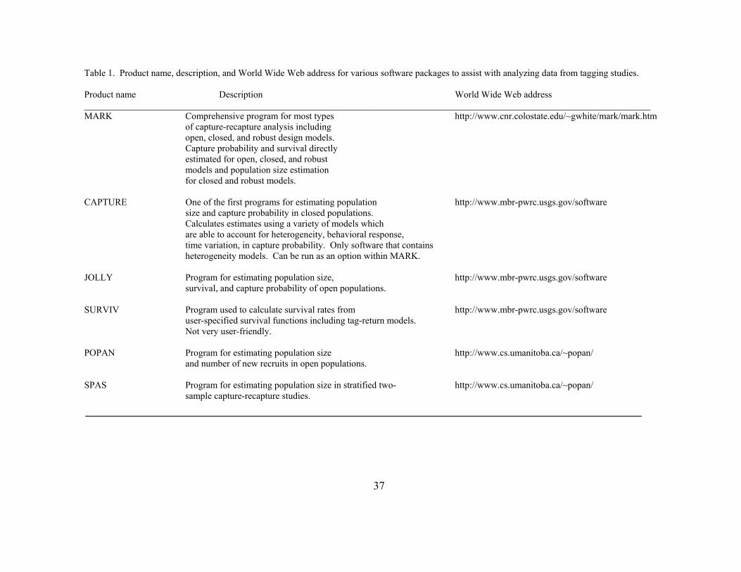
37

Table 1. Product name, description, and World Wide Web address for various software packages to assist with analyzing data from tagging studies. Product name Description World Wide Web address _________________________________________________________________________________________________________________________ MARK Comprehensive program for most types http://www.cnr.colostate.edu/~gwhite/mark/mark.htm

of capture-recapture analysis including open, closed, and robust design models. Capture probability and survival directly estimated for open, closed, and robust models and population size estimation for closed and robust models.

CAPTURE One of the first programs for estimating population http://www.mbr-pwrc.usgs.gov/software

size and capture probability in closed populations. Calculates estimates using a variety of models which are able to account for heterogeneity, behavioral response,

time variation, in capture probability. Only software that contains heterogeneity models. Can be run as an option within MARK.

JOLLY Program for estimating population size, http://www.mbr-pwrc.usgs.gov/software survival, and capture probability of open populations. SURVIV Program used to calculate survival rates from http://www.mbr-pwrc.usgs.gov/software user-specified survival functions including tag-return models. Not very user-friendly. POPAN Program for estimating population size http://www.cs.umanitoba.ca/~popan/ and number of new recruits in open populations. SPAS Program for estimating population size in stratified two- http://www.cs.umanitoba.ca/~popan/ sample capture-recapture studies.

38

Table 2. Model, type of mark required (batch or individual), source of fish used in study (research collection or fishery dependent), typical study duration, reporting rate requirement, key parameters, additional information generated, and principal software for estimating population size and mortality components from tagging models discussed in this review.

Model name Type of mark

required

Source of fish Typical study duration

Reporting rate

required?

Key demographic parameters

Additional information generated

Principal software

Lincoln-Petersen

Batch Research < 1 month No Population size Calculator, spreadsheet, SPAS

Schnabel Batch Research < 1 month No Population size Calculator, spreadsheet, or

CAPTURE Removal No mark Research < 1 month No Population size CAPTURE or

MARK Closed-

CAPTURE models

Unique individual

Research < 1 month No Population size, capture probability

CAPTURE for all closed models or MARK for non-

heterogeneity Jolly-Seber and Cormack-Jolly-

Seber

Unique individual

Research >1 month No Population size, apparent survival

Individual growth from recaptures

POPAN, JOLLY, or MARK

Robust Unique individual

Research >1 month No Population size and growth, apparent survival,

temporary emigration

Individual growth from recaptures

CAPTURE and JOLLY together

or MARK Brownie Unique

individual Fishery >1 year No Survival, total mortality BROWNIE

MARK Hoenig/ Hearn

Unique individual

Fishery >1 year Yes Survival, fishing and natural mortality

AVOCADO

Telemetry Unique individual

Research = 1 year No Survival, fishing and natural mortality

Movement, habitat use

SURVIV

Combined telemetry/ Tagging

Unique individual

Research/ Fishery

> 1 year No Survival, fishing and natural mortality

Movement, habitat use

SURVIV

39

Sampling Interval

Lincoln-Peterson

Schnabel

Closed-capture

Jolly-Seber

Robust

Figure 1. Diagram demonstrating assumptions about capture probabilities for each type of capture-recapture model discussed in this chapter. Each marker represents a sampling event. The solid lines connecting markers indicate closed populations with equal capture probabilities. Dashed lines between samples indicate closed populations with unequal capture probabilities. Gaps represent intervals where populations are open.

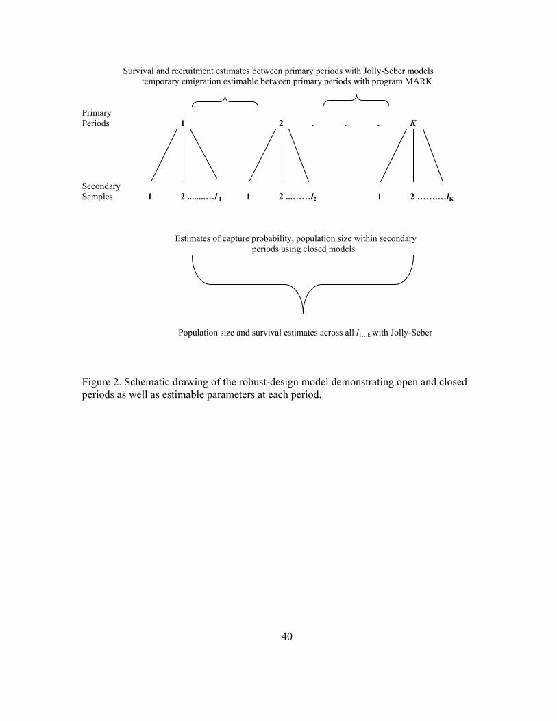
40

Survival and recruitment estimates between primary periods with Jolly-Seber models temporary emigration estimable between primary periods with program MARK

Primary Periods 1 2 . . . K Secondary Samples 1 2 ........…l 1 1 2 ...……l2 1 2 …….…lK

Estimates of capture probability, population size within secondary

periods using closed models

Population size and survival estimates across all l1…k with Jolly-Seber

Figure 2. Schematic drawing of the robust-design model demonstrating open and closed periods as well as estimable parameters at each period.

41

Box 1. Planning a capture-recapture study.

A key step in planning a capture-recapture study is to examine the possible precision

of parameter estimates before conducting the study. This helps determine if study objectives

can be met given the expected sample sizes and variances. For example, population size

estimates of an endangered species may require higher precision (as part of a recovery plan)

than estimates associated with an annually stocked game fish. One simple way to do this is

to use estimates or assumed values for capture probability and population size to generate

expected frequencies of the possible capture histories by hand (Box 1, Table 1) or on a

spreadsheet. These capture histories can then be analyzed using the software and models

discussed in this review to evaluate approximate precision at different capture histories,

population sizes, and number of samples.

As an example, there are eight (23) possible capture histories in a closed population

study with three samples. Excluding the case with no captures (000), there are seven of

interest to us (Box 1, Table 1). If we assume the capture probability (p) to be 0.10 based

either on pilot field work or published studies, and our approximate estimate of population

size (N) is 1,000 individuals, then we can calculate the expected number of fish for each

capture history (Box 1, Table 1). The expected frequencies of each capture history could

then be analyzed in MARK or CAPTURE to evaluate precision of parameter estimates using

the various closed models discussed in this review. This very simple example does not

incorporate heterogeneity. But assigning different capture probabilities to portions of the

estimated population size would simulate heterogeneity.

This approach also provides insight into the amount of effort required to obtain

precise parameter estimates. Precision can be improved by increasing the capture-probability

42

(which may be difficult), increasing the number of samples, or a combination of the two.

This allows biologists to examine if the potential gain in precision justifies the expense

associated with increasing the sampling effort.

This approach can also be generalized in two ways. We could generate expected

capture histories under a heterogeneity model and examine bias and precision of different

estimators (i.e., Mt vs. Mh). We could also generate expected capture histories under an open

model (i.e., Jolly-Seber) and examine precision issues under that scenario.

We encourage the use of simple pre-study evaluations such as this before conducting

a capture-recapture study. Biologists should find the information from these simple

simulations very useful in evaluating and planning the feasibility of a capture-recapture

study. This approach should lead to savings in both time and money by implementing the

most efficient study design and establishing realistic expectations for study results.

Box 1, Table 1

Approximate expected capture frequencies for a three sample closed population study with a capture probability p = 0.1, and estimated population size Nt = 1,000.

Capture history Formula to calculate expected frequency

Approximate expected frequency

111 p x p x p x N 1 110 p x p x (1-p) x N 9 101 p x (1-p) x p x N 9 011 (1-p) x p x p x N 9 100 p x (1-p) x (1-p) x N 81 010 (1-p) x p x (1-p) x N 81 001 (1-p) x (1-p) x p x N 81

43

CHAPTER 3

ESTIMATING POPULATION SIZE OF AN INVASIVE CATFISH IN COASTAL RIVERS

44

Abstract

Invasive aquatic species are becoming increasingly problematic for aquatic ecologists and

resource managers, as the ecological and economic impacts of introductions become better

known. The flathead catfish Pylodictis olivaris is a large piscivorous fish native to most of the

interior basin of the United States. Via legal and illegal introductions, they have been introduced

into at least 13 U.S. states and one Canadian province, primarily along the Atlantic slope. I used

a variety of capture-recapture models to estimate flathead catfish population parameters in three

North Carolina coastal plain rivers. My estimates using a Jolly-Seber model were hindered by

low capture probabilities and high temporary emigration. Reasonable estimates were calculated

using a robust-design framework for population size and temporary emigration with

supplemental information from a radio-telemetry study to examine model assumptions.

Population size estimates ranged from 4 to 31 fish/km (>125-mm total length) of sampling reach.

Additional analyses showed high rates of temporary emigration (>90%), independently

supported by radio-telemetry results. This approach to population assessment, integrating the

robust design with radio-telemetry, provides insights into demographics and behavior that are

applicable to developing a broad understanding of flathead catfish and other invasive aquatic

species.

45

Introduction

The introduction and establishment of exotic species in aquatic environments is a poorly

understood phenomenon widely considered to threaten most aquatic ecosystems. The impact of

non-native species on aquatic ecosystems is varied and unpredictable (Moyle and Light 1996).

Reported impacts of exotic species introduction range from integration into the introduced area

with no apparent impact to natives (Wikramanayake 1990), to widespread declines or extinctions

of native species and cascading negative impacts on ecosystems and their human users (Moyle

and Light 1996; Folkerts 1999; Kolar and Lodge 2000).

Knowing the abundance of an invasive species is particularly important in assessing the

“success” of the invasion, the threat of spread, or options related to potential control activities.

Estimating the relative abundances of native and exotic species within estuaries and monitoring

these populations through time was recently identified as the second highest research priority by

the U.S. National Estuarine Research Reserve System (Wasson et al. 2002). Aquatic

environments present unique challenges to researchers in assessing exotic and native species

abundance beyond those of terrestrial studies because of logistic and sampling difficulties

imposed by aquatic habitats. These sampling difficulties further exacerbate the central problem

in many capture-recapture studies of obtaining sufficient accuracy and precision in estimation

methods to develop a meaningful inference of population size.

Investigations of population dynamics often employ a wide variety of parameters,

including population size, population and individual growth rates, emigration, immigration, and

birth/death rates. Complete censuses of a population are rarely possible (Pollock et al. 1990;

Lancia et al. 1994) and determining population size of an aquatic invader is potentially more

46

difficult due to limited knowledge of the invader’s habitat use, life history, or uncertain

susceptibility to standard sampling gears.

A diverse array of models and techniques has been developed to generate estimates of

population demographics for animal populations using capture-recapture methods (Williams et

al. 2002). Under appropriate sampling conditions, these approaches are well suited to generate

accurate and precise estimates of population size and examine the population parameters (births,

deaths, immigration, emigration) shaping exotic populations.

Capture-recapture models are classified by whether the populations are open to births,

deaths, immigrants, emigrants, and permanent deletions (open models) or the population size is

constant during the study period (closed models). These models and their application are

reviewed in Chapter 2. I incorporate both approaches in this study and discuss how violations of

these assumptions affect model estimates. I also utilize auxiliary information from a concurrent

radio-telemetry study to evaluate how well the assumptions of the capture-recapture models were

met and to enhance our understanding of this aquatic invader.

Study Species

The flathead catfish Pylodictis olivaris is a large piscivorous catfish native to the Rio

Grande River, Mississippi River, and Mobile river drainages (Smith-Vaniz 1968; Jenkins and

Burkhead 1994) and introduced into at least 13 other states, including North Carolina (Jackson

1999). The only documented introduction of flathead catfish into North Carolina waters was in

1966 by an unauthorized release of 11 adults (total weight 107 kg) into the Cape Fear River near

Fayetteville (Guier et al. 1981). Within 15 years following introduction, flathead catfish had

expanded to populate a 200-km section of the river and had emerged as the dominant predator

47

within the Cape Fear River system (Guier et al. 1981). The current distribution of this species in

North Carolina includes most major river drainages.

Flathead catfish demonstrate high individual and population growth rates (Guier et al. 1981;

Quinn 1989; Munger et al. 1994; Nash and Irwin 1999), rapid range expansion (Guier et al. 1981;

Ashley and Buff 1987; Jenkins and Burkhead 1994), and carnivorous food habits (Swingle 1967;

Quinn 1989; Ashley and Buff 1987). Maximum size of flathead catfish in North Carolina (from

angling records) is currently 56% by weight of the world record collected in Kansas (31.8 kg NC;

56.4 kg KS). Stomach content analysis of this species in introduced areas has shown high

occurrence of native ictalurids, centrarchids, and clupeids (Guier et al. 1981; Ashley and Buff 1987)

leading to widespread angler and management agency concern over declining populations of native

redbreast sunfish Lepomis auritus (Guier et al. 1981; Ashley and Rachels 1998) in several rivers

along the southeastern Atlantic slope.

Given the characteristics and observations described above, resource managers in areas

where flathead catfish have been introduced are concerned with the potential impacts to native

fish communities following flathead catfish introduction. Here I examine population size for

introduced populations of flathead catfish and relate these demographic parameters to time

elapsed since each population’s introduction.

Methods

Study Sites

Three primary study rivers of similar size (mean width ~50 m each; Northeast Cape Fear

River, Cape Fear River Drainage; Contentnea Creek, Neuse River Drainage; Lumber River,

PeeDee River Drainage) located in the coastal plain region of eastern North Carolina were

48

selected for study with assistance from North Carolina Wildlife Resources Commission

(NCWRC) biologists. Flathead catfish presence in each of these rivers had been documented by

routine sampling as part of a long-term fish community monitoring conducted by NCWRC

personnel with the Northeast Cape Fear River supporting the oldest documented population

(introduced for about 30 years), followed by Contentnea Creek (about 15 years) and the Lumber

River (< 5 years). I sampled flathead catfish in fixed sample reaches adjacent to long-term

NCWRC sampling locations. Two adjacent 1-km reaches were sampled in both Contentnea

Creek and the Lumber River, and 3 adjacent 1-km reaches were sampled in the Northeast Cape

Fear River. Due to debris blocking the river (2001 and 2002) and low water conditions (2002)

in the Lumber River, one of the reaches was divided into two parts, thus catch per unit effort is

reported from three reaches in that river.

Collection

Fish were collected using low-frequency electrofishing (Smith-Root Inc. Model GPP 7.5

pulsed-DC, 1.5-2.0 A, 15 pulses/sec), a capture technique that has been shown to be the most

effective non-lethal collection technique for flathead catfish (Justus 1996; Stauffer and Koenen

1999). All flathead catfish collected were weighed (g) and measured (TL mm). Flathead catfish

>115 mm but <254 mm TL were tagged with a 12-mm Passive Integrated Transponder tag (PIT)

in the dorsal musculature behind the dorsal spine (as documented for channel catfish Ictalurus

punctatus, Moore 1992). An alternative location to the dorsal musculature was employed for

large (>254-mm TL) fish to reduce possibility of tag consumption by anglers. Fish > 254-mm

were tagged in the head musculature posterior to the eye socket with 14-mm PIT tags. Tag

insertion locations were sealed with surgical adhesive (butyl cyanoacrylate). All fish also

49

received a circular anal fin clip as a secondary batch mark to estimate tag loss. Prior to field

studies, preliminary lab experiments indicated that tag retention was high, fish behavior did not

appear to be affected by tagging, and mortality (from tag implantation or increased predation risk

due to tagging) did not appear to differ from non-tagged flathead catfish (W. E. Pine,

unpublished data).

Population Models

Because sampling efforts usually do not collect every individual in a population,

estimates of population size should incorporate a probability function of detecting an animal

(capture probability), given that the animal is available to be captured (animal is alive and

present in the sample area; Chapter 2). This capture probability is especially important in

establishing the presence of an invasive species and may be used to adjust counts of fish

collected to actual abundance by estimating animals that are present, yet not collected.

Although flathead catfish are widely distributed throughout the interior of the US and

support important recreational and commercial fisheries throughout their range (Pitlo 1997;

Travnichek and Clemmons 2001), little published information exists on their life history,

behavior, or population demographics. Because of this dearth of information, particularly related

to movement patterns, which should be considered in designing a capture-recapture study, I

initially used Jolly-Seber open population models to estimate population size (Method 1 below).

I then incorporated information from these Jolly-Seber models and auxiliary radio telemetry data

into a combined open and closed population modeling framework (Method 2 below; Pollock’s

Robust Design, Pollock 1982; Pollock et al. 1990; Chapter Two) and compared the two

approaches. Fish were collected in each reach from late spring through early fall, during the

50

times fish were susceptible to electrofishing (generally when water temperatures exceeded 18 C,

Figure 1).

Method 1: Jolly-Seber Open Models

Estimates of population size ( iN̂ ), capture probability ( $pi ), and apparent survival ( $φi )

among all samples were generated for each reach on all rivers. Low recapture rates precluded

estimation of some parameters on the Northeast Cape Fear River and many parameters on the

Lumber River.

Population size was calculated in 2001 and 2002 for each sample reach using models

developed by Cormack (1964), Jolly (1965), and Seber (1965) (Jolly-Seber models, JS) with a

general form of:

i

i

pnNi ˆ

ˆ = (1)

where:

iN̂ = estimated population size,

ni = number of marked and unmarked animals captured in the ith sample, and

ip̂ = estimated recapture probability for animals collected in the i th sample.

The population size estimates were averaged over all of the sampling periods to generate an

annual estimate of population size ( N̂ year). Estimates of population size, capture probabilities,

and associated variances were calculated using program MARK (Burnham and Anderson 1998).

Four possible open population models were fit to data from each reach in program

MARK (Table 1). These models contained two parameters, survival ( $φi ) and estimated capture

probability ( $pi ), and allowed each parameter to be either constant across all sampling events (.)

51

or variable for each sampling event (t) (Table 1). Parameter estimates were constrained between

zero and one.

Model selection was based on Akaike’s Information Criterion (AICc) (Akaike 1973)

adjusted to account for small sample size (Burnham and Anderson 1998). Parameters with

nonsensical values (e.g., infinitely large standard errors) were used as an indicator of poor model

fit to the data. I used the AICc value and biological information to select the most realistic model

with the highest precision and least amount of bias (Burnham and Anderson 1998).

Method 2: Robust Design Models

Open population models assume that all animals are equally likely to be captured in each

sampling period and any emigration is permanent (Pollock 1982; Pollock et al. 1990). These

assumptions are often difficult to meet, and several modifications to open population models

have been designed to compensate for violating the emigration assumption (Kendall et al 1999;

Williams et al. 2002). I used Pollock’s (1982) “robust design” to estimate population size within

5-day “secondary” sample periods, and open JS type models to estimate survival, immigration,

and emigration between monthly “primary” periods (Pollock 1982; Pollock et al. 1990; Kendall

et al. 1997). This sampling design requires that secondary samples are collected over short time

periods where the population is assumed closed (Chapter 2).

Traditional open population models assume that all emigration from the study area is

permanent. However natural movement patterns of the study animal can lead to situations where

individuals are entering and leaving the study reach repeatedly, creating temporary emigration

(Chapter 2). Kendall et al. (1997) described temporary emigration as either “Markovian” where

an animal “remembers” that it has left the study area and returns based on some time-dependent

52

function, or “random” where the animal leaves for one sampling event, then returns (but can

emigrate randomly again). Basically the presence of a Markovian emigrant in a sample is

dependent on the location of the animal in the previous sampling period (i.e., was the animal

available for capture in the sampled area?), whereas the presence of a random emigrant does not

depend on its location in the previous sample period. I fit models to the data collected under a

robust framework that accounted for both types of emigration.

Four robust design models were fit to each reach in each river for the 2002 data (Table 1).

I fit two “classic” robust design models; one model fixed apparent survival equal to 1, and the

other allowed survival to vary across sampling time. The classic robust models did not allow for

temporary emigration. I then fit two models incorporating temporary emigration (random, G"

and Markovian, G'). Apparent survival across primary periods was fixed at 1 for each temporary

emigration model to allow model convergence. Fishing and natural mortality were likely low for

this species over the short summer period evaluated in this study.

Incorporating radio-telemetry information

A concurrent study on flathead catfish habitat use and movement patterns in the same

study reaches in each river (NCWRC Final Report) provided important information related to

population model assumptions. Twenty-two fish were collected in Contentnea Creek, and twelve

each in the Northeast Cape Fear River and Lumber River (within the sample reaches) and

surgically implanted with radio transmitters. I used these radio-tagged fish as a known

population to help evaluate whether emigration was occurring from my study reaches and also to

empirically estimate capture probability. Capture probability was estimated by examining the

number of radio-tagged fish collected in electrofishing samples vs. the number of radio-tagged

53

fish available for capture in the sampled reach. Searches for radio-tagged fish in the sample

reaches occurred immediately after processing fish collected during the electrofishing sampling.

This auxiliary information was then incorporated when possible into population models

described above and used to evaluate population model assumptions.

Results

Catch-per-effort

During the intensive sample period from mid-May to early-September, mean catch-per-

hour was low and variable in each year at all sample reaches on each river (Table 2). Mean

flathead catfish catch-per-hour ranged from 8.8-16.6 in Contentnea Creek, 3.2-6.9 in the

Northeast Cape Fear River, and 0.3-15.2 in the Lumber River. In 2001 sampling was

concentrated in Contentnea Creek because of low capture rates in the Northeast Cape Fear and

Lumber Rivers, while in 2002 sampling was evenly distributed across rivers.

Seasonal catch rates

Catch rates varied substantially between seasons. Highest catch rates were generally

observed in each river during late spring through fall when water temperatures exceeded 18 C.

Because of low catch rates during cool seasons (Figure 1), sampling was conducted during late

spring through early fall.

Tag loss

Approximate tag loss based on recapture rates of fin-clipped fish that lost their PIT tag

show that tag loss is about 4% (2000-2002 Contentnea Creek 7 tags lost / 157 recaptures of

previously PIT tagged fish). Tag loss can positively bias population size and negatively bias

survival estimates and recapture probabilities. My population and survival estimates presented

54

are not adjusted for this minimal rate of tag loss and this should be considered in evaluating

results for all parameter estimates.

Jolly-Seber Results

Contentnea Creek

Reaches 1 and 2 were sampled 19 and 15 times, respectively, each in 2001. Ninety-six

fish were collected once in reach one, 14 were captured twice, 5 were captured three times, 1 was

captured four times, and 1 was captured five times. In reach two, 108 fish were captured once,

13 were captured twice, and 4 fish were captured three times. Unfortunately, the only model that

was able to fit the data for either reach was a fixed apparent survival and capture probability

model for reach 2 ( $.φ , $p ., Table 3, Figure 1). Other models would not fit the data because of

extremely low recapture rates and violations of several of the assumptions of open population

models (see discussion). Capture probability estimates for the model ( $pi = 0.03, SE = 0.01,

Table 3) were expectedly low given the infrequency with which I collected PIT tagged fish.

Apparent survival estimates were high ( $φ = 0.80, SE = 0.03, Table 3). However, it is not

possible to separate mortality from emigration (true survival = 1 – mortality – emigration); thus,

any emigration confounds survival estimates. Based on additional information provided by my

subset of radio-tagged fish, emigration (permanent and temporary) was occurring from sample

reaches.

Population size estimates were generated using equation 1. The mean population size for

the $.φ , $p . model (mean = 333, SE = 54, Table 3) fluctuated greatly throughout the sampling

period (Figure 2). I evaluated model sensitivity to moderate changes in apparent survival and

found that parameter estimates using these models did not change between $φ = 0.85 to 1.0.

55

My empirical estimate of capture probability for 2001 was similar to the estimate from

the $.φ , $p . model. There were 82 possible collections of radio-tagged fish in the sample reaches

(reaches 1 and 2 combined) during 2001. Only four radio-tagged fish were captured resulting in

a capture probability estimate of 0.05. Two models with this capture probability were then fit to

the data from reach 1 and 2 using MARK ( $φt , $p = 0.05 and $.φ , $p = 0.05). Only the $.φ , $p = 0.05

model from reach 2 adequately fit the data (Table 3). Survival estimates were higher for this

model ( $φ = 0.99, SE = 0.004) than for the $.φ , $p . model ( $.φ = 0.80, SE = 0.03, Table 3).

Again, this estimate is likely confounded by temporary emigration. Population size estimates

were lower for this model with mean population size = 200 (SE = 32).

Each reach was sampled 12 times during 2002, and I attempted to fit these data with Jolly-

Seber models. Forty-six fish were collected once and 12 fish were collected twice in reach 1. In

reach 2, fifty-one fish were collected once, 5 fish twice, and 2 were collected three times. For

comparative purposes, the same four open models were fit for both reaches during year two. The

only open population model that adequately fit the data was a $.φ , $p . (constant survival and capture

probability) for reach 1 in 2002. No open population model adequately fit the data for reach 2 in

2002 (parameter estimates were nonsensical). Capture probability estimates for reach 1 were

expectedly low ( $p = 0.10, SE=0.02, Table 3). Survival estimates were high for reach 1 (reach 1 $.φ

=0.95, SE = 0.02, Table 3). Population size estimates were made for the 12 samples using equation

1 (mean = 116, SE = 17, Table 3).

In 2002, 4 out of 57 possible captures of radio-tagged fish were made. Open population

models were fit to the data for reach 2 using the empirical capture probability estimate (empirical

56

$p = 0.07) . I was only able to fit a $.φ , $p = 0.07 model to the data. Survival estimates using the

empirical capture probability were higher than the $.φ , $p . model ( $.φ = 0.98, SE = 0.01). Mean

population size was similar for this reach (mean = 138, SE = 38, Table 3) as for reach 1 using a

$.φ , $p . model.

Northeast Cape Fear River

Because of low catch rates in each reach, I combined the three contiguous 1-km reaches

into a single reach. Low recaptures precluded parameter estimation using all models in 2001. In

2002, 47 fish were collected once and five fish collected twice. The $.φ , $p . model was the only

open model that fit data collected in 2002 (Table 3). Survival estimates using this model were

extremely low ( $φ = 0.02, SE = 0.04, Table 3), likely due to high emigration rates (Table 5).

Capture probability was also low ( $p = 0.04, SE = 0.02, Table 3). Estimated population size for

each km of the reach averaged 9 fish (SE = 2). As in Contentnea Creek, the radio-tagged

flathead catfish demonstrated temporary emigration occurring within the sample reach in

Northeast Cape Fear River with most radio-tagged fish leaving the sampling area for varying

time periods only to return to the sample area.

In 2002, there were 70 possible collections of radio-tagged fish in the Northeast Cape

Fear River. Only 3 of these fish were collected resulting in an empirical $p of 0.04, the same as

the model estimated $p . I fixed capture probability to the empirical estimate and re-fit the data to

the same open models as described above. Again, only the $.φ , $p 0.04 model fit, and parameter

estimates were the same as those from the $.φ , $p . model ( $φ = 0.02, SE = 0.04; N̂ = 9, SE =2,

Table 3).

57

Lumber River

Due to low catch and recapture rates, likely due to low water levels resulting from record

drought (USGS Water Resources of North Carolina), estimating population size for the Lumber

River flathead catfish population was not possible. During 2002, only 19 fish were collected

once and two fish were collected twice. Thus, a minimum population size for those reaches is 11

fish/km based on the number of fish collected divided by the river length sampled.

Meeting open-model assumptions

Because of additional insight into flathead catfish behavior provided by the subset of radio-

tagged fish, it is unlikely that any of the estimates from the open population models are accurate.

Open population models assume that any emigration is permanent. Analysis of the radio-tagged fish

movement patterns revealed flathead catfish were exhibiting temporary emigration from the study

reach in both Contentnea Creek and the Northeast Cape Fear River. The implications of this

emigration are examined in the discussion.

Robust Design Results

Contentnea Creek

2002 sampling data were collected under a robust design with month as the primary

period (four months; May, June, July, and August), and three, one-day samples within a one-

week period as the closed secondary samples each month. The best-fit model for reach 1 was the

random temporary emigration model (Table 4). Temporary emigration was very high

(temporary emigration, G" = 0.94, SE = 0.03, Table 5). Capture probability estimated with this

model was higher than with the Jolly-Seber open population model (robust design temporary

emigration model $p = 0.36, SE 0.11, Table 5). Robust design models also estimate recapture

58

probability (probability of being recaptured in the secondary sampling period). Recapture

probability ( $c ) was 0.11 (SE = 0.04, Tables 4, 5). Population size estimated for each primary

period was lower for the robust models than the Jolly-Seber open population models (N range

14-26 fish/km, Table 5, Figure 4). The classic robust design model fit nearly as well as the

random temporary emigration model (Table 4). The survival estimate under this model was low

( $φ = 0.15, SE = 0.07), likely because it was confounded with emigration (which was high).

Population size estimates were similar between the random temporary emigration model and the

classic robust model ( N̂ range 16-30 fish/km, Table 5).

The information from the radio-tagged fish was then incorporated by fitting three

additional random temporary emigration models fixing $p 0.07, $c 0.07, and both $p and $c = 0.07

while keeping $φ = 1 and allowing population size to change through time. These three models

were then compared to the best random temporary emigration described above which did not

incorporate information from the telemetered fish (Table 6). The best fit model was the random

temporary emigration model with capture probability from the radio tags ( $c 0.07) while the second

best model was the original random temporary emigration model without temporary emigration

(Table 6). Initial capture probabilities ( $p ) were the same between these two models as were

other parameter estimates (G" = 0.94, SE = 0.03; $p = 0.36, SE 0.11; N̂ range 14-26 fish/km,

Table 7). Using only the empirical capture probabilities from the radio-tagged fish ( $p 0.07, $c 0.07)

resulted in larger population size estimates ( N̂ range 20–143 fish/ km) than the other models

( N̂ range 14-26 fish/km, Table 7).

59

In reach 2, the random temporary emigration model was again the best model with high

random emigration (temporary emigration, G" = 0.93, SE = 0.02, Table 5). Estimated capture

probability was higher in reach 2 than in reach 1 ( $p = 0.53, SE 0.08, Table 5) but recapture

probability was lower ( $c = 0.01 SE = 0.01, Table 5). Population size estimates in reach 2 were

similar in size ( N̂ range 14-31 fish/km, Table 5) to reach 1 (Table 5, Figure 3).

The same three additional random temporary emigration models using information from

the radio-tag fish were also fit to the data from reach 2 as in reach 1. In reach 2, the best fitting

model did not include any fixed parameters based on information from the radio-tagged fish

(Table 6). The second best fitting model was the random temporary emigration model with fixed

capture probability from the radio tags ( $c 0.07). Again, parameter estimates were similar between

the models (G" = 0.93, SE = 0.02; $p = 0.53, SE 0.08; N̂ range 14-31 fish/km, Table 7). The

model with the highest AICc, value used only the empirical capture probabilities from the radio-

tagged fish ( $p 0.07, $c 0.07) and population size estimates were larger ( N̂ range 20–143 fish/ km)

than population estimates from the other models ( N̂ range 14-31 fish/km, Table 7).

Northeast Cape Fear River

In 2002, sampling in the Northeast Cape Fear River was conducted in a similar robust

design framework as in Contentnea Creek. The best-fit model was a classic robust design model

with fixed survival (Table 4). The survival estimate from this model was extremely low ( $φ =

0.05, SE = 0.04, Table 5), likely because of high emigration from the study reach. Capture

probability was much higher ( $p = 0.41, SE = 0.11, Table 5) than recapture probability ( $c =

0.05, SE = 0.03, Table 5). The population size range for the reach ( N̂ range 4-9 fish/km) for the

60

robust design model was similar to the mean for the open model (open model mean N̂ = 9, SE =

4, Tables 3, 5, Figure 4).

The random temporary emigration model also fit fairly well (Table 4), but gave very

different estimates. Temporary emigration was high (G" = 0.97, SE = 0.02, Table 5). Capture

and recapture probabilities were similar to the classic robust design model ( $p = 0.41, SE = 0.11;

$c = 0.05, SE = 0.03, Table 5). Population size estimates were similar to the classic robust model

( N̂ range 4-9 fish/km, Table 5, Figure 4). Although the classic robust design estimate with

fixed survival had the lowest AICc value, the random temporary emigration model is likely a

more biologically meaningful model because temporary emigration was occuring and can be

accounted for in the model.

As in Contentnea Creek, information from the radio-tagged fish was incorporated into

additional random temporary emigration models. In the Northeast Cape Fear River, the best

fitting model included a fixed $c based on recaptures of the radio-tagged fish ( $c 0.04) (Table 6).

This is similar to the results for reach 1 in Contentnea Creek. The second best fitting model was

the same random temporary emigration model as above which did not include any fixed

parameters from the radio-tagged fish. Population parameter estimates were again similar

between the models (G" = 0.97, SE = 0.02; $p = 0.41, SE 0.11; N̂ range 4-9 fish/km, Table 7).

Population estimates using only the empirical capture probabilities from the radio-tagged fish

( $p 0.04, $c 0.04) were larger ( N̂ range 26–61 fish/km) than population estimates from the other

models ( N̂ range 4-9 fish/km, Table 7).

61

Discussion

Population size estimation

Low recapture rates observed in all rivers prevented most population models from fitting

the data. These low recapture rates are possibly a function of the flathead catfish population

frequently “turning over” with the majority of the tagged fish moving out of the sampling area

and a new sub-population of fish moving in regularly. The cue for this turnover is not apparent,

but possible factors include changes in water level or prey availability. Strong annual movement

patterns appear to be related to spawning migration (NCWRC Final Report). Low catch rates are

also likely a function of poor efficiency of electrofishing gear for collecting flathead catfish in

these waters.

Temporary emigration is known to bias estimates of many population parameters

(N,φ , p ) (Pollock et al. 1990; Kendall et al. 1995; Kendall et al. 1997; Zehfuss et al. 1999). I

quantified temporary emigration under a completely random framework using the robust design.

The estimates of G" from each reach and river indicated that most tagged fish (~90%) emigrated

from the sample reach and were thus unavailable for capture at the following sample event. The

number of these PIT tagged fish that are “temporary” emigrants and later return to the sampling

reach during the sampling time is not known. Further examination of the radio-tagged fish

provides insight as to which fish are permanent emigrants and which are temporary emigrants.

The majority of radio-tagged fish in this study in each river demonstrated strong seasonal

movement patterns from the tributary to mainstem rivers beginning in late spring and

progressing through summer (NCWRC Final Report). Flathead catfish then returned to the

tributaries in the spring, only to repeat the same movement process. However, the radio-tagged

62

fish revealed temporary emigration in all rivers within the summer. In each river, individual

radio-tagged fish left for several days or weeks, and then returned to the sample reach. The

radio-tagged fish provided valuable information with which to evaluate sample design and

population model assumptions in addition to the migration and life history information provided

(NCWRC Final Report).

Burnham (1993) demonstrated that under a completely random emigration model, traditional

Jolly-Seber survival estimates are relatively unbiased by emigration, although their precision is

reduced. My survival estimates under the best Jolly-Seber models in Contentnea Creek were high

(>80%) and corresponding standard errors low (Table 3). I expected survival to be high given low

rates of angling or natural mortality, as well as the short time period (about 4 months) over which

this analysis was conducted. Although standard errors were low over the time period I evaluated,

over a longer time period the precision may be reduced as in Burnham (1993).

Kendall et al. (1997) and Kendall (1999) demonstrated that when the primary research

interest is in the “superpopulation” inhabiting the general area around the study reach that

parameters of interest ( p ,φ , N) are not biased by temporary emigration. Thus, under the

completely random emigration model, my parameter estimates within the specific primary reach

or secondary may apply to a more general area of Contentnea Creek. It is difficult to define the

geographic bounds of a superpopulation in a riverine setting. Although it is not likely that the

superpopulation in this case would characterize flathead catfish population size for the entire

Neuse River basin, it may represent a short-term carrying capacity for an area of river that offers

“desirable” habitat (e.g., based on spawning sites early in the spring or optimal deep water

structure later in the summer) at that time. For example, the general area of Contentnea Creek

63

between the upstream boundary of my sampling reach and the creek mouth (approximately 7-

km) contains about 3 km of “optimal” habitat, two of which include my sample reaches

(NCWRC Final Report). My estimates of population size and survival may apply then to a

superpopulation (the population of fish in the 3-km section of preferred habitat) in this area of

Contentnea Creek. The relationship between population size estimates collected from defined

areas (e.g., 1-km sampling reach) and an area with very large boundaries (e.g., Neuse River

system), which may contain a superpopulation, should be explored further.

One option to increase capture probability would be to increase the size of the area

sampled. However, additional analysis using combined data from the two sample reaches in

Contentnea Creek did not result in an increase in capture probability. This is likely because

flathead catfish moved a greater distance than the combined 2-km sample reach. However,

increasing the sampling area by combining the three continuous reaches in the Northeast Cape

Fear River allowed estimates to be generated, whereas individual 1-km reaches estimates were

not possible.

For some fish populations, increasing sampling effort (time expended electrofishing) may

increase capture probability, but this is not the case with flathead catfish. On several occasions I

attempted to collect additional flathead catfish known to be present in the area ( radio-tagged

fish) using multiple electrofishing passes through the sample reach. Using this approach I rarely

collected the known fish, or any additional flathead catfish. Mesa and Schreck (1989)

demonstrated that trout behavior was altered for at least 24-h following electrofishing and

marking. A similar response in flathead catfish could explain why it was difficult to capture

flathead catfish with additional sampling in the area.

64

Incorporating radio-telemetry information

I used the observed capture rates of the radio-tagged fish as empirical estimates of

capture probability and recapture probability and these estimates were similar to the $p estimates

from the Jolly-Seber models (Table 3). However, the radio-tag based estimates are not similar to

any of the $p estimates from the best robust design models (Table 5). Surprisingly, in each of

temporary emigration robust design models, the estimated $p from the radio tags is actually

much closer to the $c (recapture probability) (Table 5). In the Northeast Cape Fear River and in

reach 1 in Contentnea Creek, the additional robust design models incorporating telemetry

information were selected as the best model only if the radio-tag capture rate was used as a $c

(Table 6). Using the radio-tag capture rate as either $p or $p and $c resulted in higher AICc values

(poorer model fit) than not using the radio-tag information, or using the radio-tag information

only as a $c (Table 6). This indicates a lack of statistical support for using the empirical capture

rates from the radio tags to fit population models.

The higher capture than recapture probabilities could demonstrate a “behavioral

response” where the capture probability changes as a result of being collected previously

(Williams 2002). Several closed population models exist that can account for a behavioral

response (Chapter 2); however, the data collected in each of the primary periods here were too

sparse to fit those models. The learning ability of fish has recently been given new attention and

is likely much greater than was formerly thought (Laland et al. 2003). It may be possible that

following initial capture, flathead catfish learn to avoid collection in subsequent sampling events.

Mesa and Schreck (1989) documented that trout behavior was altered for 24 h following

electrofishing collection and tagging and a similar behavioral response could persist longer than

65

24-hours in flathead catfish. If so, my samples within the primary sampling periods (collected

48-hours apart) could be affected. The learning ability or behavioral response to sampling by

flathead catfish following electrofishing and tagging to avoid collection requires additional

research before conclusions can be drawn.

Population estimates between the model fitted $c , or the $c from the radio-tags do not

differ because initial capture probability determines the estimates of N in a robust design model

(Williams et al. 2001). However, the differences between using the model fit estimates of $p and

the $p from the radio-tags is large (Table 7). This is because in each case the $p estimates from

the radio-tags are much lower than the model fit estimates (Table 7). Given the low statistical

support for using the radio-tag $p (Table 6) and the closer agreement between the model fit $c

with the capture probability of the radio-tagged fish, the best population estimates are likely the

estimates which do not include capture or recapture probability information from the radio-

tagged fish (Tables 5, 8). However, other than a behavioral response to electrofishing and radio-

tag implementation, I am unable to speculate why $p estimates differ between the PIT-tagged

fish and the radio-tagged fish.

Comparisons to other populations

Quinn (1988) reported limited movement in an introduced flathead catfish population in

Georgia. Dames et al. (1989) and Skains and Jackson (1993) both suggest that flathead catfish

populations generally exhibit restricted movements and that relatively small river sections (2-km,

Skains and Jackson 1993) could be treated as unique management units. These reports are

similar to many fish movement studies based on tag returns or radio telemetry in that little

attention is directed to the proportion of the tagged population not recaptured (Gowan et al.

66

1994). In studies with passive tags Quinn (1988), Dames et al. (1989), and Skains and Jackson

(1993), found flathead catfish recapture rates were low (not reported, but approximately 10%,

8%, and 5%, respectively based on the number of fish recaptured / number of fish tagged in each

study) and similar to the recapture rates in this study. These authors drew their conclusions of

limited movement based on locations of recaptured fish. For example, Quinn (1988) reported

that, “…79% of recaptured flathead catfish showed no detectable movements…” but this

percentage is based on only 159 recaptures of 1,636 tagged fish. Gowan et al. (1994) review

movement studies in salmonids and other fish species and suggested that, “The large number of

fish never recaptured [in the study reach] certainly leaves open the possibility that many fish

moved beyond the boundaries.” In each of the flathead catfish studies mentioned above, the

large number of tagged fish that were never recaptured are not accounted for, possibly because

these fish had left the study area and thus were not available to be captured, similar to my results.

Skains and Jackson (1993) simultaneously used radio-tagged flathead catfish in conjunction with

their traditional passive tags in their study. These authors tagged 20 fish with radio tags, 3 of

which were immediately “lost” and were assumed to have malfunctioned, been caught and

removed, or move outside the study area. These authors searched outside of their study reaches

(ca. 30 km) for these tagged fish and did not locate them. However, given the movement

patterns I observed and other large-scale movements of flathead catfish (including tag returns

>300 km from original tagging location in 76 days, Dames et al. 1989), it is possible that several

of the “missing” fish in Skains and Jackson (1993) migrated large distances outside of the search

area.

67

Few published estimates of flathead catfish population size or density, for native or

introduced populations, exist for rivers or lakes to compare with my estimates. The flathead

catfish population sizes in the rivers I examined are within the range of published estimates for

both native and introduced populations. For native populations, Dettmers et al. (2001) report

flathead catfish densities of 0.31 and 0.53 fish/ha in Pool 26 of the Mississippi River and lower

Illinois River, respectively, from trawl samples. Orth (1980) reported flathead catfish density of

between 3-64 fish/ha (mean = 27) from Lake Carl Blackwell, Oklahoma, collected from cove

rotenone samples. In introduced populations in the Flint River, Georgia, Quinn (1988) reported

flathead catfish densities of 13 fish/ha (153 fish/river km) estimated using a Schnabel estimate

and 14 fish/ha (161 fish/km) using a Schumacher-Eschmeyer estimate. Quinn’s estimates are

much higher than abundances reported for native populations in the Missouri River (9-17

fish/km) using similar methods (Morris et al. 1971 as in Quinn (1988)). Dobbins et al. 1999

estimated the size of an introduced flathead catfish population in the Apalachicola River, Florida,

to range from 35-58 fish/km of fish ≥ 380-mm TL. Population density estimates in my study

ranged from 1-8 fish/ha (4-31 fish/km) > 125-mm TL (Table 8).

It is likely that in several of the studies above, some of the assumptions for the capture-

recapture methods used were violated in estimating population size, biasing population

estimates. Several of these studies in both native (Morris et al. 1971) and introduced populations

(Quinn 1988) used closed population estimates, which are sensitive to assumption violations.

The Schnabel and Schumacher-Eschmeyer are both closed population models that assume the

population is “closed” to births, deaths, immigration or emigration during the study period

(Chapter 2). The Quinn (1988) study took place over a six-month period from late May through

68

November. It is possible that during this period some changes in the population size occurred

from the demographic factors listed above (e.g., births or deaths). Immigration and emigration

may be less of a problem in Quinn’s (1988) study than here, given the large (50-km) study area

they used. Dobbins et al. also used a Schnabel estimator to estimate population size, and likely

met many of the assumptions of the Schnabel model by sampling relatively large areas (8.1-km

sample reaches) intensively (4-6 samples per reach) over a fairly short period (each sample

separated by 5-16 days). Dobbins et al. (1999) also carefully evaluated movement patterns of

flathead catfish within their sample sites by sampling in “buffer” zones that separated each

sample reach to check for flathead catfish movement out of each reach. The affect that violating

these assumptions would have on the population estimate would depend on which and how each

assumption is violated (Williams et al. 2002) but the most likely violations of mortality or

emigration from the study site would lead to positive biases in population size. However, even

with the potential biases in each of the above population estimates, I suspect that North Carolina

coastal rivers support flathead catfish populations that are smaller in size than introduced

populations in Georgia and Florida (Table 8).

Estimated emigration rates and observed movement patterns clearly demonstrate that my

sample reaches within tributaries are not discrete flathead catfish populations unique to each

tributary (NCWRC Final Report). I conclude that the tributary “populations” of flathead catfish

are actually extensions of populations found within each mainstem river. The information on

flathead catfish movement patterns in native and introduced populations is conflicting (some

suggest large movements (Dames et al. 1989), others do not (Dobbins et al. 1999 for an

introduced population). Based in part on my work, I clearly showed that flathead catfish in

69

coastal North Carolina rivers move extensively (NCWRC Final Report). These large movement

patterns are presumably conducive to rapid dispersal and invasion success.

Implications for presence/absence monitoring

Electrofishing appears to be a poor early indicator of flathead catfish presence or absence.

Bayley and Austen (2002) empirically estimated capture probability in ponds for a variety of fish

species using an AC boat-mounted electrofisher. For their group of several catfish species, they

estimated catchability to be 0.18%. My empirical capture probability (from the radio tags) and

estimated capture probability from the PIT-tagged fish was much higher for flathead catfish,

likely because I used direct current, lower output voltages, and pulse-rate frequency than those of

Bayley and Austen (2002). The “low-frequency” DC electrofishing technique that I used is

similar to that described by Quinn (1986) and is thought to be a more effective electrofishing

technique for collecting catfish species (Justus 1996) than the less applicable AC electrofishing

settings used by Bayley and Austen (2002).

Recommendations and conclusions

My experiences studying flathead catfish are likely similar to the difficulties encountered

in studying other invasive fish species. The low capture probability for flathead catfish

demonstrates the difficulty in detecting invasive species as a component of routine monitoring

efforts. This could result in flathead catfish not being detected in introduced areas until

populations are well established and expanding in both numbers and area occupied. By

combining the capture-recapture information from my study and telemetry information from the

larger NCWRC project, I was able to quickly learn detailed information on detection probability,

population size, movement patterns, and habitat use– critical information required to evaluate the

70

level of establishment and risk of spread of an aquatic invasive species. Further, my findings on

migration and capture probability begin to resolve seemingly conflicting results from other

flathead catfish populations. I recommend the use of a combined capture-recapture and radio

telemetry study in assessing other aquatic invasive animal populations.

The ecological impact of flathead catfish in coastal North Carolina rivers is difficult to

discern because of other confounding anthropogenic impacts on these river systems including

introduction of other exotic species, poor water quality, and habitat degradation. Flathead catfish

are well established in most major coastal North Carolina river systems and may be present at

lower densities in others as well. I had originally hoped to evaluate population size estimates in

relation to time of introduction at each of my study reaches. However, there appears to be no

clear relationship between the age of flathead catfish introduction and my estimates of

population size. While in general, Contentnea Creek appears to support slightly higher

populations than the other two rivers, the high variance of most models precludes a precise

statistical comparison.

Management efforts for flathead catfish should be focused on preventing the spread of

this species within North Carolina and elsewhere through outreach programs designed to

heighten public awareness of the threats imposed by invasive species on native fish communities.

In areas where flathead catfish have become established (such as the rivers in this study), efforts

should be made to encourage recreational and commercial harvest of this species (Chapter 5).

Given the popularity of flathead catfish as a food fish in its native and introduced range (Jackson

1999), the large recreational and commercial fisheries interest in North Carolina (National

Marine Fisheries Service 2001), the seemingly insatiable global demand for fish products, and

71

the ability of humans to impact aquatic ecosystems through intensive fishing efforts, introduced

flathead catfish may be an ideal candidate species for developing a new harvest oriented fishery.

72

References

Akaike, H. 1973. Information theory and an extension of the maximum likelihood principle, in B. Petrov and F. Cazakil editors. Proceedings of the 2nd International Symposium Information Theory, Akademiai Kidao, Budapest, Hungary.

Ashley, K. W., and B. Buff. 1987. Food habits of flathead catfish in the Cape

Fear River, North Carolina. Proceedings of the Annual Conference Southeastern Association of Fish and Wildlife Agencies 41:93-99.

Ashley, K. W., and R. T. Rachels. 1998. Changes in redbreast sunfish population

characteristics in the black and lumber rivers, North Carolina, 1994-1997. Proceedings of the Annual Conference Southeastern Association of Fish and Wildlife Agencies 52:29-38.

Bayley, P. B., and D. J. Austen. 2002. Capture efficiency of a boat electrofisher.

Transactions of the American Fisheries Society 131:435-451. Burnham, K. P., and D. R. Anderson. 1998. Model selection and inference: a

practical information-theoretic approach. Springer-Verlag, New York. Burnham, K. P. 1993. A theory for combined analysis of ring recovery and recapture

data. Pages 199-214 in J. D. Lebreton and P. M. North, editors. Marked individuals in the study of bird population. Birkhauser-Verlag, Basel, Switzerland.

Cormack, R. M. 1964. Estimates of survival from the sighting of marked animals.

Biometrika 5:429-438. Dames, H. R., T. G. Coon, and J. W. Robinson. 1989. Movements of channel and

flathad catfish between the Missouri River and a tributary, Perche Creek. Transactions of the American Fisheries Society 118:670-679.

Dettmers, J. M., S. Gutreuter, D. H. Wahl, and D. A. Soluk. 2001. Patterns in

abundance of fishes in main channels of the upper Mississippi River system. Canadian Journal of Fisheries and Aquatic Science 58:933-942.

Dobbins, D. A., R. L. Cailteux, and J. J. Nordhaus. 1999. Flathead catfish abundance

and movement in the Apalachicola River, Florida. Pages 199-201 in E. R. Irwin, W. A. Hubert, C. F. Rabini, H. L. Schramm, Jr., and T. Coon, editors. Catfish 2000: proceedings of the international ictalurid symposium. American Fisheries Society, Symposium 24, Bethesda, Maryland.

73

Folkerts, G. W. 1999. State and fate of the world’s aquatic fauna. Pages 1-16 in G. W. Benz and D. E. Collins, editors. Aquatic fauna in peril: the southeastern perspective. The Southeastern Aquatic Research Institute Special Publication Number 1. Lenz Design and Communications, Inc., Decatur, Georgia.

Funk, J. L. 1955. Movement of stream fishes in Missouri. Transactions of the American

Fisheries Society 85:39-57. Gowan, C, M. K. Young, K. D. Fausch, S. C. Riley. 1994. Restricted movement in

resident salmonids: a paradigm lost?. Canadian Journal of Fisheries and Aquatic Sciences 51:2626-2637

Guier, R. C., L. E. Nichols, and R. T. Rachels. 1981. Biological investigation of

flathead catfish in the Cape Fear River. Proceedings of the Annual Conference Southeastern Association of Fish and Wildlife Agencies 35:607-621.

Jackson, D. C. 1999. Flathead catfish: biology and management. Pages 23-36 in E.

R. Irwin, W. A. Hubert, C. F. Rabini, H. L. Schramm, Jr., and T. Coon, editors. Catfish 2000: Proceedings of the international ictalurid symposium. American Fisheries Society, Symposium 24, Bethesda, Maryland.

Jenkins, R. E., and N. M. Burkhead. 1994. Freshwater fishes of Virginia. American

Fisheries Society, Bethesda, Maryland. Jolly, G. M. 1965. Explicit estimates from capture-recapture data with both death and

immigration stochastic model. Biometrika 52:225-247. Justus, B. 1996. Observations on electrofishing techniques for three catfish species in

Mississippi. Proceedings of the Annual Conference Southeastern Association of Game and Fish Commissioners 48:524-532.

Kolar, C. S. and D. L. Lodge. 2000. Freshwater nonindigenous species: interactions

with other global changes. in H. A. Mooney and R. J. Hobbs, editors. Invasive species in a changing world. Island Press, Washington, D.C.

Kendall, W. L., and J. D. Nichols. 1995. On the use of secondary capture-recapture

samples to estimate temporary emigration and breeding proportions. Journal of Applied Statistics 22:751-762.

Kendall, W. L., J. D. Nichols, and J. E. Hines. 1997. Estimating temporary

emigration using capture-recapture data with Pollock’s robust design. Ecology 78: 563-578.

74

Kendall, W. L. 1999. Robustness of closed capture-recapture methods to violations of the closure assumption. Ecology 80:2517-2525.

Laland, K. N., C. Brown, and J. Krause. 2003. Learning in fishes: From three-second

memory to culture. Fish and Fisheries 4:199-202. Lancia, R. A., J. D. Nichols, and K. H. Pollock. 1994. Estimating the number of

animals in wildlife populations. Pages 215-253 in T. A. Bookhout, editor. Techniques for Wildlife and Habitats, 5th edition. The Wildlife Society, Bethesda, Maryland.

Mesa, M. G., and C. B. Schreck. 1989. Electrofishing mark-recapture and depletion

methodologies evoke behavioral and physiological changes in cutthroat trout. Transactions of the American Fisheries Society 118:644-658.

Moore, A. 1992. Passive integrated transponder tagging of channel catfish.

The Progressive Fish-Culturist 54:125-127. Moyle, P. B. and T. Light. 1996. Biological invasions of fresh water: Empirical rules and

assembly theory. Biological Conservation 78:148-161. Munger, C. R., G. R. Wilde, and B. J. Follis. 1994. Flathead catfish age and size at

maturation in Texas. North American Journal of Fisheries Management 14:403-408. Nash, M. K., and E. R. Irwin. 1999. Use of otoliths versus pectoral spines for aging

adult flathead catfish. Pages 309-316 in E. R. Irwin, W. A. Hubert, C. F. Rabini, H. L. Schramm, Jr., and T. Coon, editors. Catfish 2000: proceedings of the international ictalurid symposium. American Fisheries Society, Symposium 24, Bethesda, Maryland.

National Marine Fisheries Service. 2001. 2000 fisheries of the United States. B.

K. O’Bannon, editor. National Marine Fisheries Service, Office of Science and Technology, Fisheries Statistics and Economics Division. Silver Spring, Maryland.

Otis, D. L., K. P. Burnham, G. C. White, and D. R. Anderson. 1978. Statistical

inference from capture data on closed populations. Wildlife Monographs 62. Orth, D. J. 1980. Changes in fish community of Lake Carl Blackwell, OK (1967-1977)

and a test of the reproductive guild concept. Proceedings of the Oklahoma Academy of Science 60:10-17.

Pitlo, J., Jr. 1997. Response of upper Mississippi River channel catfish populations to

changes in commercial harvest regulations. North American Journal of Fisheries Management 17:848-859.

75

Pollock, K. H. 1982. A capture-recapture design robust to unequal probability of capture. Journal of Wildlife Management 46:757-760.

Pollock, K. H., J. D. Nichols, C. Brownie, and J. E. Hines. 1990. Statistical inference

for capture-recapture experiments. Wildlife Monographs 107. Quinn, S. P. 1986. Effectiveness of an electrofishing system for collecting flathead

catfish. Proceedings of the Annual Conference Southeastern Association of Fish and Wildlife Agencies 40:85-91.

Quinn, S. P. 1988. Stomach contents of flathead catfish in the Flint River, Georgia.

Proceedings of the Annual Conference of Southeastern Associate of Fish and Wildlife Agencies 41(1987):85-92.

Quinn, S. P. 1989. Flathead catfish abundance and growth in the Flint River, Georgia.

Proceedings of the Annual Conference Southeastern Association of Fish and Wildlife Agencies. 42:141-148.

Seber, G. A. F. 1965. A note on the multiple recapture census. Biometrika 52:249-259. Skains, J. A., and D. C. Jackson. 1995. Linear ranges of large flathead catfish in two

Mississippi streams. Proceedings of the Annual Conference of Southeastern Association of Fish Wildlife Agencies 42:141-148.

Smith-Vaniz, W. F. 1968. Freshwater fishes of Alabama. Auburn University

Agricultural Experiment Station. Paragon Press, Montgomery, Alabama. Stauffer, K. W. and B. D. Koenen 1999. Comparison of methods for sampling flathead

catfish in the Minnesota river. Pages 329-339 in E. R. Irwin, W. A. Hubert, C. F. Rabini, H. L. Schramm, Jr., and T. Coon, editors. Catfish 2000: proceedings of the international ictalurid symposium. American Fisheries Society. Symposium 24, Bethesda, Maryland.

Swingle, H. S. 1967. Experiments with the flathead catfish (“Pylodictis olivaris”) in

ponds. Proceedings of the Annual Conference Southeastern Association of Game and Fish Commissioners. 18:303-308.

Thomas, M. E. 1993. Monitoring the effects of introduced flathead catfish on sport fish populations in the Altamaha River, Georgia. Proceedings of the Annual Conference Southeastern Association of Fish and Wildlife Agencies 47:531-538.

Travnickek, V. H. and H. D. Clemmons. 2001. Utility of tournament data for assessing

effects of eliminating commercial catfish harvest in the Missouri river. North American Journal of Fisheries Management 21:688-691.

76

Wasson, K., D. Lohrer, M. Crawford, S. Rumrill. 2002. Non-native species in our

nation’s estuaries: A framework of an invasion monitoring program. National Estuarine Research Reserve System. Technical Report Series 2002:1.

Wikramanayake, E. D. 1990. Conservation status of the endemic rain forest fishes of

Sri Lanka: results of a translocation experiment. Conservation Biology 4:32-37. Williams, B. K., J. D. Nichols, and M. J. Conroy. 2002. Analysis and management of

animal populations: modeling, estimation, and decision making. Academic Press, San Diego, California.

Zehfuss, K. P., J. E. Hightower, and K. H. Pollock. 1999. Abundance of Gulf sturgeon in

the Apalachicola River, Florida. Transactions of the American Fisheries Society 128: 130-143.

77

Table 1. Name and description of each model fit to capture-recapture data collected in each river during either 2001, 2002, or both.

Model Description

Open Models

MARK Φ(t), p(t) Survival and capture probability variable, parameters constrained from 0 to 1

MARK Φ(t), p(.) Survival varies with time, capture probability fixed, parameters constrained from 0 to 1

MARK Φ(.), p(t) Survival fixed, capture probability varies with time, parameters constrained from 0 to 1

MARK Φ(.), p(.) Survival and capture probability fixed, parameters constrained from 0 to 1

Robust Design Models

Φ =1, p(..), $c (..), Nt, E=0, I=0 Classic robust design

Survival=1, fixed capture and recapture probability, population size varies for each primary period, no emigration or immigration, parameters constrained from 0 to 1

Φ(..), p(..), $c (..), Nt, E=0, I=0 Classic robust design

Survival, capture and recapture probability fixed, population size varies for each primary period, no emigration or immigration, parameters constrained from 0 to 1

Φ = 1, p(..), $c (..), Nt, E.t, I. Robust design with Markovian temporary emigration

Survival=1, capture and recapture probability fixed, population size varies for each primary period, Markovian temporary emigration, parameters constrained from 0 to 1

Φ =1, p(..), $c (..), Nt, E. = I. Robust design with random temporary emigration

Survival=1, capture and recapture probability fixed, population size varies for each primary period, random temporary emigration, parameters constrained from 0 to 1

78

Table 2. Year, river, sample reach, number of sampling days, mean catch-per-unit-effort (CPUE, fish/hour), and standard error (SE) of flathead catfish catch for each river during 2001 and 2002. All samples were collected using low-frequency electrofishing described in text. Low water in the Lumber River in 2002 prevented sampling in reach 3.

Year River Reach Number of sampling days

Mean CPUE (SE)

2001 Contentnea 1 18 9.04 (4.49) 2001 Contentnea 2 18 16.62 (8.23) 2002 Contentnea 1 12 8.77 (2.53) 2002 Contentnea 2 12 11.15 (2.35)

2001 Northeast Cape Fear 1 10 5.11 (1.27) 2001 Northeast Cape Fear 2 10 6.93 (2.01) 2001 Northeast Cape Fear 3 10 5.33 (1.82) 2002 Northeast Cape Fear 1 12 3.95 (0.82) 2002 Northeast Cape Fear 2 12 4.70 (1.73) 2002 Northeast Cape Fear 3 12 3.23 (0.80)

2001 Lumber 1 8 3.52 (1.30) 2001 Lumber 2 9 3.66 (1.22) 2001 Lumber 3 6 9.46 (1.79) 2002 Lumber 1 12 2.25 (1.01) 2002 Lumber 2 12 0.32 (0.22) 2002 Lumber 3 1 15.25 (0.00)

79

Table 3. Open population model results for each year, river, and reach where an open model was able to fit the data. Estimated capture probability ( $p ), survival ( $φ ), and mean population size per kilometer over the summer sampling period and associated standard errors are shown. Population estimates are biased by temporary emigration (see text).

Year River Reach Open Population Model $p (SE) Survival (SE) Summer period mean N/km (SE)

2001 Contentnea 2 $.φ , p.

Fixed survival, capture probability 0.03 (0.01) 0.80 (0.03) 333 (54)

2001 Contentnea 2 $.φ , p 0.05

Fixed survival, empirical capture probability 0.05 based on radios

0.99 (0.004) 200 (32)

2002 Contentnea 1 $.φ , p.

Fixed survival, capture probability 0.10 (0.02) 0.95 (0.02) 116 (17)

2002 Contentnea 2 $.φ , p 0.07

Fixed survival, empirical capture probability 0.05 based on radios

0.99 (0.01) 138 (38)

2002 NECFR All $.φ , p.

Fixed survival, capture probability 0.04 (0.02) 0.02 (0.04) 9 (2)

80

Table 4. River, reach, model name, AICc value, delta AICc, AICc weight, and number of model parameters for each robust design model fit to the data. Bold indicates best-fit model with lowest AICc value and highest AICc weight.

River Reach Robust Design Model AICc Delta AICc AICc Weight Number of parameters

Contentnea 1 $φ = 1, p.., $c .., Nt, E=0, I=0 Classic robust design

13.43 4.98 0.05 6

Contentnea 1 $.φ , p.., $c .., Nt, E=0, I=0

Classic robust design

10.18 1.73 0.24 7

Contentnea 1 $φ = 1, p.., $c .., Nt, E.t, I. Markovian temporary emigration

11.21 2.75 0.14 9

Contentnea 1 $φ = 1, p.., $c .., Nt, E. = I. Random temporary emigration

8.45 0.00 0.57 7

Contentnea 2 $φ = 1, p.., $c .., Nt, E = 0, I = 0 Classic robust design

-32.46 20.22 0.00 6

Contentnea 2 $.φ , p.., $c .., Nt, E = 0, I = 0

Classic robust design

-30.13 22.55 0.00 7

Contentnea 2 $φ = 1, p.., $c .., Nt, E.t, I. Markovian temporary emigration

-51.76 0.92 0.39 8

Contentnea 2 $φ = 1, p.., $c .., Nt, E. = I. Random temporary emigration

-52.7 0.00 0.61 6

NECFR ALL $φ = 1, p.., $c .., Nt, E=0, I=0 Classic robust design

-2.85 9.55 0.01 6

NECFR ALL $.φ , p.., $c .., Nt, E=0, I=0

Classic robust design

-12.40 0.00 0.78 7

NECFR ALL $φ = 1, p.., $c .., Nt, E.t, I. Markovian temporary emigration

-6.87 5.53 0.05 9

NECFR ALL $φ = 1, p.., $c .., Nt, E. = I. Random temporary emigration

-9.27 3.13 0.16 7

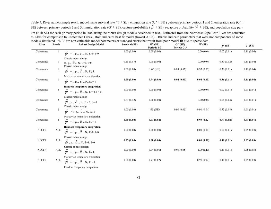
81

Table 5. River name, sample reach, model name survival rate (Φ ± SE), emigration rate (G″ ± SE ) between primary periods 1 and 2, emigration rate (G″ ± SE) between primary periods 2 and 3, immigration rate (G′ ± SE), capture probability ( $p ± SE), recapture probability ( $c ± SE), and population size per-km (N ± SE) for each primary period in 2002 using the robust design models described in text. Estimates from the Northeast Cape Fear River are converted to 1-km for comparison to Contentnea Creek. Bold indicates best fit model (lowest AICc). Blanks indicate parameters that were not components of some models simulated. “NE” are non-estimable model parameters or standard errors that result from poor model fit due to sparse data.

River Reach Robust Design Model Survival (SE) G'' (SE) Periods 1-2

G'' (SE) Periods 2-3

G' (SE) $p (SE) $c (SE)

Contentnea 1 $φ = 1, p.., $c .., Nt, E=0, I=0

Classic robust design

1.00 (0.00) 0.00 (0.00) 0.00 (0.0) 0.02 (0.01) 0.11 (0.04)

Contentnea 1 Φ., p.., $c .., Nt, E=0, I=0 Classic robust design

0.15 (0.07) 0.00 (0.00) 0.00 (0.0) 0.30 (0.12) 0.11 (0.04)

Contentnea 1 $φ = 1, p.., $c .., Nt, E.t, I.

Markovian temporary emigration

1.00 (0.00) 1.00 (NE) 0.89 (0.07) 0.97 (0.03) 0.36 (0.11) 0.11 (0.04)

Contentnea 1 $φ = 1, p.., $c .., Nt, E. = I.

Random temporary emigration

1.00 (0.00) 0.94 (0.03) 0.94 (0.03) 0.94 (0.03) 0.36 (0.11) 0.11 (0.04)

Contentnea 2 $φ = 1, p.., $c .., Nt, E = 0, I = 0

Classic robust design

1.00 (0.00) 0.00 (0.00) 0.00 (0.0) 0.02 (0.01) 0.01 (0.01)

Contentnea 2 $.φ , p.., $c .., Nt, E = 0, I = 0

Classic robust design

0.81 (0.42) 0.00 (0.00) 0.00 (0.0) 0.04 (0.04) 0.01 (0.01)

Contentnea 2 $φ = 1, p.., $c .., Nt, E.t, I.

Markovian temporary emigration

1.00 (0.00) NE (NE) 0.90 (0.05) 0.91 (0.04) 0.53 (0.08) 0.01 (0.01)

Contentnea 2 $φ = 1, p.., $c .., Nt, E. = I.

Random temporary emigration

1.00 (0.00) 0.93 (0.02) 0.93 (0.02) 0.53 (0.08) 0.01 (0.01)

NECFR ALL $φ = 1, p.., $c .., Nt, E=0, I=0

Classic robust design

1.00 (0.00) 0.00 (0.00) 0.00 (0.00) 0.01 (0.01) 0.05 (0.03)

NECFR ALL $.φ , p.., $c .., Nt, E=0, I=0

Classic robust design

0.05 (0.04) 0.00 (0.00) 0.00 (0.00) 0.41 (0.11) 0.05 (0.03)

NECFR ALL $φ = 1, p.., $c .., Nt, E.t, I.

Markovian temporary emigration

1.00 (0.00) 0.94 (0.06) 0.95 (0.05) 1.00 (NE) 0.41 (0.11) 0.05 (0.03)

NECFR ALL $φ = 1, p.., $c .., Nt, E. = I.

Random temporary emigration

1.00 (0.00) 0.97 (0.02) 0.97 (0.02) 0.41 (0.11) 0.05 (0.03)

82

Table 5. Continued. River Reach Robust Design Model N (SE), May N (SE), June N (SE), July N (SE), August

Contentnea 1 $φ = 1, p.., $c .., Nt, E=0, I=0 Classic robust design

226 (129) 411 (219) 349 (189) 287 (159)

Contentnea 1 $.φ , p.., $c .., Nt, E=0, I=0

Classic robust design

16 (5) 30 (9) 26 (8) 21 (7)

Contentnea 1 $φ = 1, p.., $c .., Nt, E.t, I. Markovian temporary emigration

14 (3) 27 (6) 22 (5) 18 (4)

Contentnea 1 $φ = 1, p.., $c .., Nt, E. = I. Random temporary emigration

14 (3) 26 (6) 22 (5) 18 (4)

Contentnea 2 $φ = 1, p.., $c .., Nt, E = 0, I = 0 Classic robust design

410 (159) 190 (83) 308 (123) 58 (35)

Contentnea 2 $.φ , p.., $c .., Nt, E = 0, I = 0

Classic robust design

279 (282) 129 (133) 209 (213) 39 (44)

Contentnea 2 $φ = 1, p.., $c .., Nt, E.t, I. Markovian temporary emigration

31 (3) 14 (2) 23 (2) 4 (NE)

Contentnea 2 $φ = 1, p.., $c .., Nt, E. = I. Random temporary emigration

31 (3) 14 (2) 23 (2) 4 (NE)

NECFR ALL $φ = 1, p.., $c .., Nt, E=0, I=0 Classic robust design

322 (79) 199 (49) 169 (43) 138 (36)

NECFR ALL $.φ , p.., $c .., Nt, E=0, I=0

Classic robust design

9 (2) 5 (1) 4 (1) 4 (1)

NECFR ALL $φ = 1, p.., $c .., Nt, E.t, I. Markovian temporary emigration

9 (1) 16 (3) 13 (3) 11 (2)

NECFR ALL $φ = 1, p.., $c .., Nt, E. = I. Random temporary emigration

9 (2) 5 (1) 4 (1) 4 (1)

83

Table 6. River, reach, model name, AICc value, delta AICc, AICc weight, and number of model parameters for random temporary emigration robust design models fit to data collected in 2002. Models were fit with and without empirical estimates of capture and recapture probability from radio-tagged fish. Bold indicates best-fit model with lowest AICc value and highest AICc weight.

River Reach Robust Design Model AICc Delta AICc AICc Weight Number of parameters

Contentnea 1 $φ = 1, p.., $c .., Nt, E. = I. 8.45 1.04 0.31 7

Contentnea 1 $φ = 1, p 0.07, $c .., Nt, E. = I. 11.60 4.19 0.06 6

Contentnea 1 $φ = 1, p.., $c 0.07, Nt, E. = I. 7.41 0.00 0.52 6

Contentnea 1 $φ = 1, p 0.07, $c 0.07, Nt, E. = I. 10.64 3.22 0.10 5

Contentnea 2 $φ = 1, p.., $c .., Nt, E. = I. -52.68 0.00 0.92 6

Contentnea 2 $φ = 1, p 0.07, $c .., Nt, E. = I. -35.25 17.43 0.0002 6

Contentnea 2 $φ = 1, p.., $c 0.07, Nt, E. = I. -47.85 4.83 0.08 6

Contentnea 2 $φ = 1, p 0.07, $c 0.07, Nt, E. = I. -30.42 22.26 0.00001 5

NECFR ALL $φ = 1, p.., $c .., Nt, E. = I. -9.27 2.56 0.20 7

NECFR ALL $φ = 1, p 0.04, $c .., Nt, E. = I. -4.01 7.82 0.01 6

NECFR ALL $φ = 1, p.., $c 0.04, Nt, E. = I. -11.83 0.00 0.73 6

NECFR ALL $φ = 1, p 0.04, $c 0.04, Nt, E. = I. -6.46 5.37 0.05 5

84

Table 7. River name, sample reach, model name survival rate ( $φ + SE), emigration rate (G″ + SE ) between primary periods 1 and 2, emigration rate (G″ +

SE) between primary periods 2 and 3, capture probability ( $p + SE), recapture probability ( $c + SE), and population size per-km (N+ SE) for each primary period in 2002 using the random temporary emigration model with and without capture probability information from radio tags. Bold indicates best fit model (lowest AICc). Blanks indicate parameters that were not components of some models simulated. “NE” are non-estimable model parameters or standard errors that result from poor model fit due to sparse data.

River Reach Robust Design Model Survival (SE) G'' (SE) Periods 1-2

G'' (SE) Periods 2-3

$p (SE) $c (SE)

Contentnea 1 $φ = 1, p.., $c .., Nt, E. = I. 1.00 (0.00) 0.94 (0.03) 0.94 (0.03) 0.36 (0.11) 0.11 (0.04)

Contentnea 1 $φ = 1, p 0.07, $c .., Nt, E. = I. 1.00 (0.00) 0.77 (0.11) 0.77 (0.11) 0.07 (NE) 0.11 (0.04)

Contentnea 1 $φ = 1, p.., c 0.07, Nt, E. = I. 1.00 (0.00) 0.94 (0.03) 0.94 (0.03) 0.36 (0.11) 0.07 (NE)

Contentnea 1 $φ = 1, p 0.07, $c 0.07, Nt, E. = I. 1.00 (0.00) 0.77 (0.11) 0.77 (0.11) 0.07 (NE) 0.07 (NE)

Contentnea 2 $φ = 1, p.., $c .., Nt, E. = I. 1.00 (0.00) 0.93 (0.02) 0.93 (0.02) 0.53 (0.08) 0.01 (0.01)

Contentnea 2 $φ = 1, p 0.07, $c .., Nt, E. = I. 1.00 (0.00) 0.68 (0.11) 0.68 (0.11) 0.07 (NE) 0.01 (0.01)

Contentnea 2 $φ = 1, p.., $c 0.07, Nt, E. = I. 1.00 (0.00) 0.93 (0.02) 0.93 (0.02) 0.53 (0.08) 0.01 (0.01)

Contentnea 2 $φ = 1, p 0.07, $c 0.07, Nt, E. = I. 1.00 (0.00) 0.68 (0.11) 0.68 (0.11) 0.07 (NE) 0.07 (NE)

NECFR ALL $φ = 1, p.., $c .., Nt, E. = I. 1.00 (0.00) 0.00 (0.00) 0.01 (0.01) 0.05 (0.03)

NECFR ALL $φ = 1, p 0.04, $c .., Nt, E. = I. 1.00 (0.00) 0.00 (0.00) 0.41 (0.11) 0.05 (0.03)

NECFR ALL $φ = 1, p.., $c 0.04, Nt, E. = I. 1.00 (0.00) 0.94 (0.06) 0.95 (0.05) 0.41 (0.11) 0.05 (0.03)

NECFR ALL $φ = 1, p 0.04, $c 0.04, Nt, E. = I. 1.00 (0.00) 0.97 (0.02) 0.41 (0.11) 0.05 (0.03)

85

Table 7. Continued.

River Reach Robust Design Model N (SE), May N (SE), June N (SE), July N (SE), August Contentnea 1 $φ = 1, p.., $c .., Nt, E. = I. 14 (3) 26 (6) 22 (5) 18 (3)

Contentnea 1 $φ = 1, p 0.07, $c .., Nt, E. = I. 56 (15) 102 (21) 86 (19) 71 (17)

Contentnea 1 $φ = 1, p.., $c 0.07, Nt, E. = I. 14 (3) 26 (6) 22 (5) 18 (3)

Contentnea 1 $φ = 1, p 0.07, $c 0.07, Nt, E. = I. 56 (15) 102 (21) 86 (19) 71 (17)

Contentnea 2 $φ = 1, p.., $c .., Nt, E. = I. 31 (3) 14 (2) 23 (2) 4 (NE)

Contentnea 2 $φ = 1, p 0.07, $c .., Nt, E. = I. 143 (24) 66 (17) 107 (21) 20 (9)

Contentnea 2 $φ = 1, p.., $c 0.07, Nt, E. = I. 31 (3) 14 (2) 23 (2) 4 (NE)

Contentnea 2 $φ = 1, p 0.07, $c 0.07, Nt, E. = I. 143 (24) 66 (17) 107 (21) 20 (9)

NECFR ALL $φ = 1, p.., $c .., Nt, E. = I. 9 (2) 5 (1) 4 (1) 4 (1)

NECFR ALL $φ = 1, p 0.04, $c .., Nt, E. = I. 61 (12) 37 (6) 32 (9) 26 (8)

NECFR ALL $φ = 1, p.., $c 0.04, Nt, E. = I. 9 (2) 5 (1) 4 (1) 4 (1)

NECFR ALL $φ = 1, p 0.04, $c 0.04, Nt, E. = I. 61 (12) 37 (10) 32 (9) 26 (8)

86

Table 8. Flathead catfish population biomass and density with associated standard error and approximate 95% confidence intervals (±2 SE) estimated for each river, reach, and month. Estimates were made using the best population estimate for each reach (see text) and average flathead catfish weights for that month of sampling.

Year River Reach Month Biomass (kg/km)

SE 95% Confidence

interval

Biomass(kg/ha)

SE 95% Confidence

interval

Density(N/km)

SE 95% Confidence

interval

Density (N/ha)

SE 95% Confidence

interval 2002 Contentnea 1 May 38.4 37.5 0 – 113.4 12.4 21.3 0 – 66.8 14 3 8 – 20 5 1.7 1.1 – 7.9 2002 Contentnea 1 June 54.9 72.0 0 – 198.9 17.8 41.0 0 – 126.9 26 6 14 – 38 8 3.4 1.6 – 15.2 2002 Contentnea 1 July 46.0 57.4 0 – 160.8 14.9 32.6 0 – 99.9 22 5 12 – 32 7 2.8 1.4 – 12.8 2002 Contentnea 1 August 21.8 31.9 0 – 85.6 7.1 18.2 0 – 49.9 18 3 10 – 26 6 2.3 1.3 – 10.4 2002 Contentnea 2 May 65.7 60.05 0 – 185.8 5.0 16.6 0 – 43.5 31 3 25 – 37 2 0.8 0.7 – 4.0 2002 Contentnea 2 June 21.7 31.3 0 – 84.3 1.7 8.7 0 – 20.1 14 2 10 – 18 1 0.6 0 – 2.2 2002 Contentnea 2 July 35.0 44.33 0 – 123.6 2.7 12.3 0 – 28.6 23 2 18 – 26 2 0.6 0.6 – 2.8 2002 Contentnea 2 August 5.6 NE NE 0.4 NE 0 – 4.4 4 NE NE 0.3 NE NE 2002 NECFR All May 7.5 12.3 0 – 32.2 0.7 3.7 0 – 9.2 9 0.8 0 – 19 2 1.5 0 – 3.8 2002 NECFR All June 1.8 3.6 0 – 8.9 0.2 1.1 0 – 2.4 5 0.5 0 – 11 1 0.9 0 – 2.3 2002 NECFR All July 3.5 4.7 0 – 12.9 0.3 1.4 0 – 3.6 4 0.4 0 – 10 1 0.9 0 – 2.2 2002 NECFR All August 2.3 3.3 0 – 90. 0.2 1.0 0 – 2.4 4 0.3 0 – 8 1 0.6 0 – 1.5

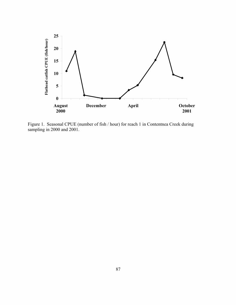
87

0

5

10

15

20

25

Flat

head

cat

fish

CPU

E (f

ish/

hour

)

Figure 1. Seasonal CPUE (number of fish / hour) for reach 1 in Contentnea Creek during sampling in 2000 and 2001.

August 2000

December April October 2001

88

0

100

200

300

400

500

600

700

800

900

Num

ber

of fi

sh /

kmSite 1Site 2

Figure 2. Open population model estimates for reach 1 and reach 2 in Contentnea Creek during 2001. Population estimates are biased by temporary emigration although population trends may be accurate (see text).

May June July August

89

0

5

10

15

20

25

30

35

May June July August

Num

ber

of fi

sh /

km

0

5

10

15

20

25

30

35

May June July August

Num

ber

of fi

sh /

km

Figure 3. Estimated population size (+ SE) for each sample reach during each primary period from Contentnea Creek during 2002 using the best fit model (see text), a robust design model with random temporary emigration.

Site 2

Site 1

90

0

5

10

15

20

25

30

35

May June July August

Num

ber

of fi

sh /

km

Figure 4. Estimated population (+ SE) size of sample reach during each primary period from the Northeast Cape Fear River during 2002 using the best fit model (see text), a classic robust design model with fixed survival.

91

CHAPTER 4

FOOD HABITS OF INTRODUCED FLATHEAD CATFISH

92

Abstract

I found that in three North Carolina coastal rivers (Contentnea Creek, Northeast Cape

Fear River, Lumber River), over two years, flathead catfish fed on a wide variety of

freshwater fish and invertebrates, anadromous fish, and occasionally estuarine fish and

invertebrates. Fish or crayfish comprised more than 50% of the stomach contents by percent

occurrence, percent-by-number, and percent-by-weight in all rivers and years. A significant

difference in the diet composition percent-by-number was found between Contentnea Creek

and the Northeast Cape Fear River (p < 0.0001). Significant differences were not found

between years within Contentnea Creek (p = 0.32) but were found within the Northeast Cape

Fear River (p = 0.009). Feeding intensity (as measured by stomach fullness) was highest in

the Northeast Cape Fear River and was associated with a lower mean size of feeding flathead

catfish in this river than in those in Contentnea Creek or the Lumber River. This may be

because of an allometric bias in the stomach fullness index used which does not account for

small fish having a proportionally larger stomach size : fish body size ratio than large fish. A

significant correlation between diet item length and flathead catfish total length was found

for Contentnea Creek in 2001 (R = 0.221, p = 0.006) but not in 2002 (R = -0.053, p = 0.435).

This relationship was not significant in the Northeast Cape Fear River in either year (2001 R

= 0.15, p = 0.24; 2002 R = -0.05, p = 0.67). Based on the diet composition data collected in

this study and those published on native and introduced flathead catfish populations, I am not

able to support or refute the hypothesis that flathead catfish are preferentially feeding on

specific species or families. However, the flathead catfish populations examined here are

well established, and the greatest impact from selective predation may have occurred

immediately following introduction. Based on my findings, flathead catfish could restructure

93

or suppress native fish communities in coastal rivers through direct predation because of their

primarily piscivorous food habits.

Introduction

The flathead catfish Pylodictis olivaris is a large piscivorous catfish native to the Rio

Grande, Mississippi, and Mobile river drainages (Smith-Vaniz 1968; Jenkins and Burkhead

1994) and has been introduced by legal and illegal means into at least 13 states and one

Canadian province (Jackson 1999). The only known flathead catfish introduction into North

Carolina waters occurred in 1966 when 11 adults (total weight 107 kg) were released into the

Cape Fear River near Fayetteville, North Carolina (Guier et al. 1981). Within 15 years the

flathead catfish distribution had expanded to cover a 200-km section of the river, and it had

emerged as the dominant predator within the Cape Fear River system (Guier et al. 1981).

Flathead catfish demonstrate high individual and population growth rates (Guier et al.

1981; Quinn 1989; Munger et al. 1994; Nash and Irwin 1999), rapid dispersal (Guier et al. 1981;

Ashley and Buff 1987; Jenkins and Burkhead 1994), and carnivorous food habits (Swingle 1967;

Quinn 1989; Ashley and Buff 1987). Individual flathead catfish growth rates in introduced

populations are generally higher than those in native riverine systems, but are similar to those

reported in reservoirs (Guier et al. 1981; Quinn 1989; Munger et al. 1994). Maximum size of

flathead catfish in North Carolina (from angling records) is currently 56% of the world record

collected in Kansas (31.8 kg NC; 56.4 kg KS).

Throughout their introduced range, feeding patterns of flathead catfish have been widely

studied to discern their impact on native fish communities. Swingle (1967) documented that

flathead catfish >254-mm TL “may compete with fishermen for fish of harvestable size” in

ponds. Results from studies such as those of Swingle (1967), as well as widespread angler

94

concern over declining populations of native sport fishes following flathead catfish introductions,

have led several state agencies to study flathead catfish food habits in the fish’s introduced range.

Several of these studies generally suggest a decline in native fish populations following

introduction of flathead catfish (Guier et al. 1981; Thomas 1995) while others detected no

impact on native fisheries following introduction (Ashley and Buff 1987; Quinn 1987).

Information on native fish community composition prior to invasion is usually limited

for any given area, and introduced species introductions often occur simultaneously with

other anthropogenic impacts that may alter native fish abundance (Townsend and Crowl

1991; White and Harvey 2001). This phenomenon often results in a time-series bias, where

the present fish assemblage suffers from the “ghost of predation past” (i.e., the impact

resulting from predation pressure that occurred in the past remains evident) such that any

potential impact on native species by the introduced species occurred prior to the study.

Further, it may be assumed that declines in native species are the result of species (i.e.,

flathead catfish) introduction, when it is also possible that a suite of biotic (e.g., poor

recruitment) or anthropogenic abiotic changes could alter fish assemblage composition

(Williamson 1997; White and Harvey 2001).

In this chapter, I examine diet patterns in introduced populations of flathead catfish

from three coastal river systems in North Carolina and compare these results to published

foraging information for native and other introduced flathead catfish populations. It is

widely thought that invasive species, at least initially, exploit an abundance of prey types that

did not co-evolve with the mode of predation by the invader (Moyle and Light 1996a, b). I

attempt to ascertain if foraging patterns exist that fit current conceptual models of invasive

species foraging theory to address this question: do introduced flathead catfish selectively

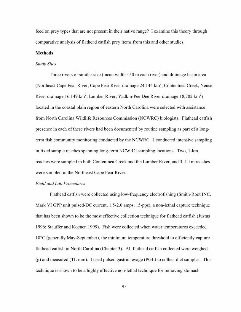
95

feed on prey types that are not present in their native range? I examine this theory through

comparative analysis of flathead catfish prey items from this and other studies.

Methods Study Sites Three rivers of similar size (mean width ~50 m each river) and drainage basin area

(Northeast Cape Fear River, Cape Fear River drainage 24,144 km2; Contentnea Creek, Neuse

River drainage 16,149 km2; Lumber River, Yadkin-Pee Dee River drainage 18,702 km2)

located in the coastal plain region of eastern North Carolina were selected with assistance

from North Carolina Wildlife Resources Commission (NCWRC) biologists. Flathead catfish

presence in each of these rivers had been documented by routine sampling as part of a long-

term fish community monitoring conducted by the NCWRC. I conducted intensive sampling

in fixed sample reaches spanning long-term NCWRC sampling locations. Two, 1-km

reaches were sampled in both Contentnea Creek and the Lumber River, and 3, 1-km reaches

were sampled in the Northeast Cape Fear River.

Field and Lab Procedures Flathead catfish were collected using low-frequency electrofishing (Smith-Root INC.

Mark VI GPP unit pulsed-DC current, 1.5-2.0 amps, 15-pps), a non-lethal capture technique

that has been shown to be the most effective collection technique for flathead catfish (Justus

1996; Stauffer and Koenen 1999). Fish were collected when water temperatures exceeded

18°C (generally May-September), the minimum temperature threshold to efficiently capture

flathead catfish in North Carolina (Chapter 3). All flathead catfish collected were weighed

(g) and measured (TL mm). I used pulsed gastric levage (PGL) to collect diet samples. This

technique is shown to be a highly effective non-lethal technique for removing stomach

96

contents from flathead catfish (>95% effective, Waters et al. 2003). Stomach contents were

individually labeled, sealed, and placed on wet ice. All extracted diet materials were

returned to the laboratory and frozen. Prior to analysis samples were thawed, and extracted

stomach contents identified to the lowest possible taxon, blotted and weighed wet (± 0.01 g),

then measured along the longest axis (± 0.5 mm). Items that were not identifiable to family

(e.g., a few bones, scales, or pieces of tissue) were grouped as either unidentified fish or

unidentified invertebrates.

Stomach contents were quantified using several standard techniques (Bowen 1996).

The frequency of occurrence of prey items was measured by compiling a cumulative list of

all of the families found in the stomach contents. I then recorded the presence or absence of

each stomach item from the list for each fish. For example, if 23 of the 84 flathead catfish

stomachs with contents examined in Contentnea Creek during 2002 contained the family

Cambaridae, then the frequency of occurrence of Cambaridae was 0.27 or 27%.

I also examined the percent composition by number of stomach contents for

individual fish by calculating the percent composition of each prey group in the flathead

catfish stomachs, and then calculating a mean percent composition value for each group in

each year and river. I then pooled the samples for each year by river and used a repeated

measures multivariate analysis of variance (MANOVA) to compare diet composition by

number between rivers (years combined) and between years within each river. In this

comparison, the treatment was river or year, the repeatedly measured response variable was

percent by number of each prey group in the stomach contents, and the replicates were

individual fish within each river. The Lumber River was not included in this analysis

because of low sample sizes.

97

Stomach fullness was calculated ([stomach contents wet weight/fish wet body weight]

x 100) as a measure of feeding intensity and reported as a percent of the flathead catfish

weight. Correlations between stomach item length and fish TL were examined for trends in

prey size and fish size in each river and year. Percent composition by weight of stomach

contents was summed across all flathead catfish prey items in each year and river and

presented as mean weights of each prey group by year and river.

Results

Most stomach items were highly digested and often difficult to identify.

Identification to the family level was common and each family was considered a group for

analysis (Table 1). Flathead catfish have a well developed jaw and pharyngeal teeth, which

masticated many of the food items when eaten. Unidentifiable material in the stomach

contents was classified as unidentified fish or unidentified invertebrates and included as a

group (similar to family) for analysis. Typical unidentified contents included pieces of fish

flesh, scales, bones, or spine fragments. Unidentified invertebrates were usually pieces of

insect wing, thorax, or legs.

Contentnea Creek

Flathead catfish in Contentnea Creek were primarily piscivorous with fish comprising

the majority of stomach contents by frequency of occurrence, percent by number, and weight

each year (Tables 2-4). In 2001, stomach contents from 176 fish were examined, of which

80 contained food items (45%) from 7 identifiable fish families and 4 invertebrate families.

In 2002, contents from 158 stomachs were examined, and 84 contained food items (53%)

from 6 fish families and 5 invertebrate families. Unidentifed fish material was the most

common prey item by occurrence (57.5%) and number (49.0%) (Tables 2 and 3), but the

98

group Centrarchidae (mostly Lepomis spp., “sunfish”) was the most common item by weight

(48.2%, Table 4). On average, individual prey items from the group Percidae (perch and

darters) were the largest by weight (Table 5, mean = 28.5 g), although this average was

heavily skewed by one large yellow perch Perca flavescens (168 g). If this yellow perch was

not included, the group Centrarchidae would be the largest by weight. Similar results were

found in 2002 for frequency of occurrence (Table 1, unidentified fish = 45.4%), percent-by-

number (Table 2, unidentifiable fish = 45.39%), and percent total weight (Table 3,

unidentifiable fish = 48.2%, Tables 1-3). Sunfish were the heaviest individual prey item

(Table 4, mean = 14.5 g). The group Cambaridae (crayfish) was also a common prey item by

occurrence, number, and total weight (Tables 2, 3). In 2001, crayfish ranked second in both

occurrence (Table 2, 26.3%) and number (Table 3, 18.7%) and were fourth in weight (Table

4, 3.91%). In 2002, crayfish were again the second most commonly occurring stomach item

(Table 2, 19.3%), the third most common item by number (Table 3, 13.6%) and by total

weight (Table 4, 10.1%). Diet percent composition was not significantly different between

years (Wilks’ Lambda F 14,149 = 1.16, p = 0.32). Feeding intensity as measured by stomach

fullness was low (<1.0 % of flathead catfish body weight) and variable during 2001 and 2002

in Contentnea Creek (Table 6). The relationship between flathead catfish total length and

diet item length was significant in 2001 (R = 0.22, p= 0.006, Figure 1) but was not significant

in 2002 (R = -0.05, p = 0.43, Figure 1).

Northeast Cape Fear River

Stomachs of flathead catfish from the Northeast Cape Fear contained primarily

crayfish and fish material from unknown families. In 2001, stomach contents from 100

flathead catfish were examined, of which 29 contained food items (29.0%) from 3

99

identifiable fish and 4 invertebrate families. In 2002 contents from 115 stomachs were

examined, and 58 contained food items (50.4%) from 2 identifiable fish and 3 invertebrate

families. In 2001, unidentified fish material was the most common prey item by occurrence

(Table 2, 55.2%) and number (Table 3, 38.8%), but sunfish were the most common item by

total weight (Table 4, 45.9%). Sunfish were also the largest prey item by weight (Table 5,

mean = 9.49 g). In 2002, crayfish were the leading stomach item by frequency of occurrence

(Table 2, crayfish = 60.3%), number (Table 3, crayfish = 53.4%), and percent total weight

(Table 4, crayfish = 52.4%). Sunfish were the largest prey group by average weight (Table

5, mean = 8.08 g). Overall in 2001, all fish material comprised about 50% of the stomach

contents by occurrence, number, and total weight, while invertebrates (primarily crayfish)

were the dominant items in 2002. Diet percent composition was significantly different

between years (MANOVA Wilks’ Lambda F 9, 77 =2.68, p = 0.009). Feeding intensity in the

Northeast Cape Fear River was also low (stomach fullness range 0.2 - 3.8%) and variable

during 2001 and 2002 (Table 6). No correlation was detected between flathead catfish total

length and stomach item length in 2001 (R = 0.15, p = 0.24, Figure 1) or 2002 (R = -0.45, p =

0.67, Figure 1).

Lumber River

Flathead catfish catch rates in the Lumber River were low (Chapter 3) which reduced

sample sizes for diet analyses and eliminated the Lumber River from some analyses. In

2001, stomach contents from 23 fish were analyzed, and 7 of these contained prey items

(30.4%) from 1 identifiable fish and 1 invertebrate group. In 2002, 24 stomachs were

analyzed, and 15 contained prey items (62.5%) from 2 identifiable fish and 2 invertebrate

families. As in the other rivers, stomach contents were primarily composed of unidentified

100

fish remains and crayfish. Unidentified fish were the most common stomach item in 2001 by

occurrence (Table 2, 57.1%) and number (Table 3, 47.6%) while sunfish were the most

common group by weight (Table 4, 51.8%) and the largest group by mean weight (0.66 g).

In 2002, unidentified fish were the most common group by occurrence (Table 2, 60.0%),

while crayfish were the most common group by number (Table 3, 48.1%), and Ictaluridae

(catfish) by weight (Table 4, 55.8%). Ictalurids were also the largest item by mean weight

(Table 5, mean = 27.9 g). Feeding intensity in the Lumber River was low (Table 6, stomach

fullness range 0.0001 - 0.95 %).

Summary and Between Year and River Comparison

Diet percent composition between Contentnea Creek and the Northeast Cape Fear

River was significantly different (MANOVA Wilks’ Lambda F 15, 245 = 4.71, p < 0.0001).

Because of low sample sizes, the Lumber River was not included in this comparison. The

percent-by-number data show that the two most common food types were either unidentified

fish material (4 of 6 estimates) or crayfish (2 of 6 estimates). The results from the percent-

by-number results correspond well with the frequency of occurrence results; most flathead

catfish are consuming other fish in their diet (Table 3), and the most commonly occurring

prey items were fish material. Fish material comprised >50% of all stomach items in 5 of the

6 estimates. The MANOVA results between years within each river are clearly supported by

closely examining the frequency-by-number data. In Contentnea Creek, the ranked

composition of the diet material by number did not change between 2001 and 2002 (Table 3)

and the MANOVA test for differences in percent-by-number of each group was not

significant (p = 0.32). However, in the Northeast Cape Fear River, the rankings of the diet

composition changed fairly dramatically between years from unidentified fish as the leading

101

group with about 39% of the total diet to crayfish as number one in 2002 with about 53% of

the diet (Table 3). As a result of this change, the MANOVA between 2001 and 2002 was

significant (p = 0.009).

Discussion

Identification of stomach contents may be difficult due to digestion of the prey item

between the time it is consumed by the predator and sampled by the researcher (Bowen 1996). I

found a high frequency of empty stomachs, low stomach fullness values, and highly digested

condition of most stomach contents that made identification below the family level difficult.

This also biased my assessment of the actual length or weight of a prey item towards an

underestimate. Bowen (1996) recommended collecting fish for diet analysis when their

stomachs are at the fullest. Minckley and Deacon (1959) found the highest average number of

organisms in flathead catfish stomachs in fish collected between 6:30 a.m. and 12:30 p.m., which

includes the time period I collected most of my samples. Bowen (1996) also cautioned that some

capture gears may cause fish to regurgitate their stomach contents. I used low frequency

electrofishing to collect my fish and occasionally noticed some regurgitation of food while fish

were being held in the live-well prior to processing. However, the amount of regurgitated

material observed was low, and I attempted to minimize collection stress and process collected

fish as rapidly as possible to minimize regurgitation.

My frequency of occurrence data (Table 2), clearly demonstrate that more than 50% of

flathead catfish consume other fish. In 5 of 6 estimates (3 rivers x 2 years), other fish (identified

families + unidentified fish) were found in more than 85% of the flathead catfish stomachs with

food items. Of the identified fish families, sunfish frequently occurred in each river and year and

were found in the top 3 in occurrence ranking in 4 of the 6 estimates (Table 2).

102

Crayfish occurrence ranked either first or second in all estimates. Invertebrates were

found in less than 50% of flathead catfish stomachs in 5 of the 6 estimates. Six other

invertebrate families were identified in stomach contents, but occurrences of these families were

rare. Surprisingly, juvenile marine shrimp (Penaidae, most likely white shrimp Litopenaeus

setiferus) were found in about 7% of the flathead catfish stomachs in Contentnea Creek but were

not found in stomach contents from the other rivers. It is not clear where flathead catfish

encountered these prey items, because Contentnea Creek is about 25 km from the beginning of

the Neuse River estuary, the closest known white shrimp habitat. As soft-bodied invertebrates,

the digestion rate of shrimp would be rapid (Bowen 1996). It is highly unlikely that a flathead

catfish consuming shrimp in the estuary and then swimming the 25-km to Contentnea Creek

would not fully digested these items. Flathead catfish must be encountering white shrimp much

closer then the Neuse River estuary, perhaps within the mainstem Neuse River via a counter-

current river flow which may be transporting small marine invertebrates up river. The use of

marine derived food items by flathead catfish is discussed in more detail below and warrants

further investigation.

The percent-by-weight data were not compiled on an individual fish level, but were

instead pooled by river and year because the condition of the stomach items was more conducive

to assessing prey size from length that weight. For example, a complete fish spine in the

stomach contents provided an adequate estimate of the minimum length of the fish prey eaten,

but it would not provide a good indicator of the weight of the prey item. Unidentified fish or

crayfish were usually the leading prey groups from the frequency of occurrence (Table 2) and the

percent-by-number analysis (Table 3). When I examine the overall contribution of the various

prey groups by weight (Table 4), fish material again contributes more than 70% of the diet by

103

weight in 5 of the 6 estimates and it usually (4 of 5) contributes more than 85% of the diet by

weight. This is further evidence that fish provides most of the food items to flathead catfish.

The largest prey groups by weight are usually in the family Centrarchidae, Percidae, and

Ictaluridae based on the percent-by-weight data and the mean weight of prey items data (Table

5). Although crayfish often ranked first or second by occurrence and frequency, by percent

weight and average weight they usually ranked third or forth (Tables 4, 5).

Because most stomach contents were highly digested, feeding intensity as measured by

stomach fullness was often < 1.0 (Table 7). In seven of the nine month x year x river

combinations when more than one estimate of stomach fullness was available for each river, the

Northeast Cape Fear River had the highest stomach fullness values of the three rivers (Table 6).

In these seven instances, the mean size of the flathead catfish with stomach contents was lower

in the Northeast Cape Fear than the other rivers (Table 6). These results are likely because of an

allometric bias in the stomach fullness index used, which has been documented for several fish

species across a range of sizes (Kwak et al. 1992) where the stomach size : fish size ratio is

larger for small fish. This could also indicate that smaller fish may be feeding more intensively

than larger fish. Weight- specific metabolic demands increase with decreasing size (Diana

1995). Also, as fish grow larger they may switch prey types or sizes of prey (Werner and Hall

1974). A combination of either of these could be occurring with flathead catfish in these rivers

and affecting estimates of feeding intensity. Differential feeding intensity by size classes of

flathead catfish should be explored further.

Often as predator size increases, prey size increases to a certain level until predators

begin to make choices related to prey availability, handling time, and energy value of the prey

(Diana 1995). This is likely true for flathead catfish. However, I found few large prey items in

104

the stomach contents although there was indications from some items (such as large scales) from

larger flathead catfish that came from large prey items.

Flathead catfish stomachs from Contentnea Creek contained twice as many identifiable

fish families as did those from the Northeast Cape Fear River. Although the comparison

between Contentnea Creek and the Lumber River was not performed due to low numbers of

stomach samples from the Lumber River, flathead catfish from Contentnea Creek had six times

as many identifiable fish families as did flathead catfish in the Lumber River. Of the 16 prey

groups considered here (14 identifiable prey families, 2 unidentifiable groups) only six were

common between the Northeast Cape Fear River and Contentnea Creek in 2001 and 2002, and of

these six, two were the unidentified fish and invertebrate groups. The MANOVA result also

serves as supporting evidence for the ecological conclusion that flathead catfish in Contentnea

Creek fed on a wider range of prey types than in the Northeast Cape Fear River. Although not

supported by a statistic, the same conclusion is apparent between the Lumber River and

Contentnea Creek (Tables 2, 3); flathead catfish fed on a wider range of prey types in Contentena

Creek.

My results are similar to an early study describing flathead catfish feeding patterns

(Minckley and Deacon 1959) who found that the “Kinds [sic] of foods eaten {by flathead

catfish} evidently depended on its [sic] availability.” Similar to findings in native systems

(Layher and Bloes 1980; Roell and Orth 1992), crayfish were also commonly consumed by

flathead catfish in my study (Tables 2-3). Roell and Orth (1992) estimated that flathead catfish

consumed 10% of the annual production of age-1 and age-2 crayfish in the New River, West

Virginia. The frequency of crayfish occurrence in flathead stomachs may be somewhat biased

by the slow digestion rate of the hard crayfish exoskeleton. Bowen (1996) cautioned that slowly

105

digested prey items may accumulate in the digestive system of a predator relative to more rapidly

digested items. Even if crayfish remains accumulated in the digestive tract of flathead catfish

and positively biased crayfish abundance in the diet, they are still likely an important component

of flathead catfish diet.

Juvenile anadromous shad were found in flathead catfish stomachs in Contentnea

Creek (Tables 1-3). As part of other fisheries research sampling efforts within the Neuse

River basin, flathead catfish were incidentally collected and found to be feeding on adult

hickory shad Alosa mediocris (J. Hightower, North Carolina State University unpublished

data). Ashley and Buff (1987) also found adult anadromous shad in flathead stomachs from

the Cape Fear River, North Carolina. Adult shad were not present in the rivers I sampled

during the time periods I could effectively collect flathead catfish. Within their native and

introduced range flathead catfish have been documented to forage heavily on juvenile and

adult gizzard shad Dorosoma cepedianum (Layer and Bloes 1980; Quinn 1987). This further

indicates that adult clupeids do not pose gape limitations to adult flathead catfish. The

impacts of flathead catfish predation on juvenile and adult anadromous shad could be

important to managers involved with anadromous shad restoration efforts along the Atlantic

slope. This is explored further in Chapter 5.

The overall contribution of marine-derived prey items to flathead catfish diets in this

study (i.e., shrimp, hogchokers Trinectes maculatus, and anadromous shad) is relatively low

(Tables 1-3) but potentially ecologically important. MacAvoy et al. (2000) examined the use

of marine derived nutrients by blue catfish Ictalurus furcatus, an introduced omnivore in the

James River, Virginia using stable isotope techniques. These authors found that introduced

blue catfish derived a significant proportion of their nutrition from spawning anadromous

106

Alosa spp. (MacAvoy et al. 2001) and suggested that the impact of introduced piscivores

along the Atlantic coast be examined.

Comparisons among flathead catfish diet studies

Prey species are thought to be unusually vulnerable to the predation style of a newly

introduced predator (Williamson 1996; Moyle and Light 1996a). Guier et al. (1981) reported

large abundance changes (by change in percent composition by weight of total population

biomass) in the native fish community in the Cape Fear River, North Carolina following

flathead catfish introduction. The largest changes were found in the native ictalurids,

primarily brown bullheads Ameiurus nebulosus and flat bullheads Ictalurus platycephalus.

Bluegill Lepomis macrochirus, black crappie Pomoxis nigromaculatus, and blue catfish were

the most frequently occurring items found in flathead catfish stomachs by Guier et al. 1981

(and all of these species were found in samples from my study). Ashley and Buff (1986) in

a follow-up study to that of Guier et al. (1981) found that “…there is no evidence to support

anglers’ claims that flathead catfish may be responsible for the reputed decline in sunfish

populations….” Moser and Roberts (1999) did not collect any native ictalurids in river

reaches to examine the effects of introduced ictalurids and recreational electrofishing on

ictalurid populations in the Cape Fear River. It is possible that flathead catfish and blue

catfish extirpated native ictalurids in the section of the Cape Fear studied by Moser and

Roberts (1999). Ashley and Rachels (1998) noted a decline in electrofishing catch rates for

native red breast sunfish in the Black and Lumber rivers, North Carolina, and considered

predation by flathead catfish as a possible reason for this decline.

Quinn (1987) examined diet patterns in the introduced flathead catfish population in

the Flint River, Georgia and suggested, “…adverse impacts on traditional fisheries are

107

unlikely,” based on findings that small flathead catfish fed primarily on crayfish and darters

(Etheostoma spp.), and larger flatheads fed on gizzard shad Dorosoma cepedianum, sunfish

(Lepomis spp.), and suckers (Catostomidae). In the Altamaha River, Georgia, Thomas

(1995) documented an 80% decline in redbreast sunfish abundance and near elimination of

native bullheads following flathead catfish introduction. Over the same time period,

electrofishing catch rates for flathead catfish increased nearly 400%. This led Thomas

(1995) to implicate flathead catfish as the cause for changes in the Altamaha River’s fish

assemblage. In other lotic systems with introduced flathead populations such as the

Ocmulgee River, Georgia, abundances of silver redhorse Moxostoma anisurum, robust

redhorse M. robustum, snail bullhead Ameiurus brunneus, flat bullhead, and redbreast sunfish

were all negatively correlated with flathead catfish presence and abundance likely due to

direct predation by flathead catfish (Bart et al. 1994). Silver redhorse is the only species of

this group found in the native range of flathead catfish.

Flathead catfish may be contributing to the decline of the federally threatened Gulf

sturgeon Acipenser oxyrinchus desotoi in the Apalachicola River, Florida by consuming

young sturgeon (Fuller et al. 1999). Flathead catfish are not native to the Apalachicola River,

but flathead catfish and Gulf sturgeon distributions overlap in rivers west of Mobile Bay (i.e.,

Pearl River, Mississippi). Flathead catfish are also thought to be contributing to the decline

of the federally endangered razorback sucker Xyrauchen texanus in the San Pedro River,

Arizona, due to intensive predation on juveniles, and are likely to prevent re-establishment of

this species in its native range (Marsh and Brooks 1989). Fuller et al. (1999) considered the

introduction of flathead catfish as probably the most biologically harmful of all fish

introductions in North America.

108

My results correspond well with general trends from a range of published studies

examining flathead catfish feeding patterns. Juvenile flathead catfish generally prey

intensively on invertebrates when small, and then feed on progressively larger prey items

(mostly fish) as they grow larger (Minckley and Deacon 1959). These results are similar,

and based on my findings and other published studies, it appears that flathead catfish are

obligate carnivores that prefer fish prey.

When I examine the few piscine prey items identifiable in my study to species from

all the rivers combined, flathead catfish preyed both on species which co-evolved with them

and species which did not. The paradigm that introduced predators selectively feed on prey

species unfamiliar with a particular predation style is not strongly supported or refuted from

my diet information alone, or by the published information on flathead catfish diets (see

above). Indirect evidence demonstrating a correlation in declines of specific prey species

with the introduction of flathead catfish found in other studies supports the hypothesis that

flatheads may affect certain species or families. Direct evidence of flathead catfish

selectively feeding on a prey species may be difficult to ascertain given the variety of animal

prey items and the difficulty I encountered in identifying stomach contents. However, the

impact of the additional predation pressure from flathead catfish, even at low levels, may

exceed the sustainable mortality level for a particular prey species population; a modeling

exercise may further resolve this hypothesis (Chapter 5).

In both Contentnea Creek and the Northeast Cape Fear River, flathead catfish have a

broader range of available forage items, including anadromous and estuarine species, than

those in the Lumber River. These species may serve as a predation buffer to resident native

freshwater fishes by diffusing flathead catfish predation pressure across a larger prey base.

109

This finding supports the suggestion by Ashley and Rachels (1998) that declines in native

redbreast sunfish (which did not co-evolve with flathead catfish) populations observed in the

Lumber River may be a result of direct predation by flathead catfish, because fewer potential

prey types are available in the Lumber River than in the other rivers I examined.

Future work

Quantitative evaluation of prey selectivity by flathead catfish would provide clearer

insight into whether flathead catfish selectively prey on certain species or families.

However, this evaluation is difficult to accomplish, not only because of the limitations in

readily identifying stomach contents I observed, but other logistic reasons as well. I was able

to estimate the relative proportion of prey items in the stomach contents, yet it is much more

difficult to define the relative abundance of prey items that were available as prey to flathead

catfish. Ideally, prey abundance estimates would need to be quantified simultaneously with

flathead catfish diet samples. Even if the abundance of potential prey items was quantified

with the diet samples, this does not necessarily describe the abundance of prey organisms

encountered by feeding flathead catfish. Diurnal monitoring of radio-tagged flathead catfish

would provide insight into the habitat types flathead catfish are most active in, possibly

providing insight into the habitat areas and times that should be sampled to evaluate what

prey are available to flathead catfish while they are feeding. Some salmonids are known to

feed on invertebrates during the nighttime invertebrate drift and shift to feeding on fish

during the day (Bowen 1996). The flathead catfish diet composition in this study may be

similarly diurnal, with flathead catfish feeding at night on crayfish (when crayfish are

emergent from burrows) and on other fish either at night or during the day. A diel

110

comparison of stomach samples from several 24-hour sampling periods may help answer this

question.

The use of marine prey items by flathead catfish is an important area of research that

should be explored. Comparative stable isotope studies of flathead catfish isotopic signatures

in areas accessible to estuarine environments and in areas separated from marine

environments (e.g., above dams) would provide insight into the extent of use of marine-

derived resources. Sonic telemetry of flathead catfish in areas adjacent to estuarine

environments coupled with diet sampling as in my study could provide information on the

extent of estuarine habitat use and feeding by flathead catfish. This result is particularly

important to resource managers concerned with anadromous fish stocks and in managing

marine species that use estuarine environments as nursery areas where juveniles may be

susceptible to flathead catfish predation.

Conclusions and management implications

I have shown that introduced flathead catfish in coastal North Carolina are primarily

piscivorous and feed on a wide variety of fish families. Flathead catfish also frequently

consume crayfish, another important component of their diet. Many of the fish families I

found in the flathead catfish diet contain species that represent important recreational

fisheries in coastal North Carolina rivers such as bluegill sunfish, largemouth bass, red breast

sunfish, and anadromous shad. Other families represented in the diet contain species of

special concern due to their imperiled population status. Based on the findings of this study

and from reviewing published flathead catfish food habits papers, I am not able to clearly

confirm or refute the hypothesis that flathead catfish selectively feed on certain prey species

including recreationally important sportfishes or species which did not co-evolve with

111

flathead catfish. However, the flathead catfish populations examined here are established,

reproducing populations, and if selective feeding by flathead catfish did occur, the impact

would likely be greatest initially following introduction. Restoration and management efforts

for native fish communities should consider the presence of invasive species, such as flathead

catfish, in coastal Atlantic slope rivers. The presence of a voracious predator such as

flathead catfish could hamper the success of these efforts via direct predation of species of

interest to managers.

112

References

Ashley, K. W., and B. Buff. 1987. Food habits of flathead catfish in the Cape Fear River, North Carolina. Proceedings of the Annual Conference Southeastern Association of Fish and Wildlife Agenices 41:93-99.

Ashley, K. W., and R. T. Rachels. 1998. Changes in redbreast sunfish population

characteristics in the black and lumber rivers, North Carolina, 1994-1997. Proceedings of the Annual Conference Southeastern Association of Fish and Wildlife Agenices 52:29-38.

Bowen, S. H. 1996. Quantitative descript of the diet. Pages 513-532 in B. R. Murphy

and D. W. Willis, editors. Fisheries techniques, 2nd edition. American Fisheries Society, Bethesda, Maryland.

Diana, J. S. 1995. Biology and ecology of fishes. Cooper Publishing Group, Carmel,

Indiana. Foster, J. R. 1977. Pulsed gastric lavage: an efficient method of removing the

stomach contents of live fish. The Progressive Fish-Culturist 39:166-169. Fuller, P. L., L. G. Nico, and J. D. Williams. 1999. Nonindigenous fishes

introduced into inland waters of the United States. American Fisheries Society, Special Publication 27, Bethesda, Maryland.

Guier, R. C., L. E. Nichols, and R. T. Rachels. 1981. Biological investigation of

flathead catfish in the Cape Fear River. Proceedings of the Annual Conference Southeastern Association of Fish and Wildlife Agencies 35:607-621.

Jackson, D. C. 1999. Flathead catfish: biology and management. Pages 23-36

in E. R. Irwin, W. A. Hubert, C. F. Rabini, H. L. Schramm, Jr., and T. Coon, editors. Catfish 2000: proceedings of the international ictalurid symposium. American Fisheries Society, Symposium 24, Bethesda, Maryland.

Jenkins, R. E., and N. M. Burkhead. 1994. Freshwater fishes of Virginia.

American Fisheries Society, Bethesda, Maryland. Kwak, T. J., M. J. Wiley, L. L. Osborne, and R. W. Larimore. 1992. Application of

diel feeding chronology to habitat suitability analysis of warmwater stream fishes. Canadian Journal of Fisheries and Aquatic Sciences 49:1417-1430.

Layher, W. G., and R. J. Boles. 1980. Food habits of the flathead catfish, Pylodictis

olivaris (Rafinesque), in relation to length and season in a large Kansas reservoir. Transactions of the Kansas Academy of Sciences 83:200-214.

113

MacAvoy, S. E., S. A. Macko, S. P. McIninch, and G. C. Garman. 2000. Marine nutrient contributions to freshwater apex predators. Oecologia 122:568-573.

MacAvoy, S. E., S. A. Macko, and G. C. Garman. 2001. Isotopic turnover in aquatic

predators: quanitifying the exploitation of migratory prey. Canadian Journal of Fisheries and Aquatic Science 58:923-932.

Marsh, P. C., and J. E. Brooks. 1989. Predation by ictalurid catfishes as a deterrent to

re-establishment of hatchery-reared razorback suckers. Southwestern Naturalist 34:188-195.

Minckley, W. L., and J. E. Deacon. 1959. Biology of the flathead catfish in Kansas.

Transaction of the American Fisheries Society 88:344-355.

Moser, M. L., and S. B. Roberts. 1999. Effects of nonindigenous ictalurids and recreational electrofishing on the ictalurid community of the Cape Fear River drainage, North Carolina. Pages 479-486 in E. R. Irwin, W. A. Hubert, C. F. Rabini, H. L. Schramm, Jr., and T. Coon, editors. Catfish 2000: proceedings of the international ictalurid symposium. American Fisheries Society, Symposium 24, Bethesda, Maryland.

Moyle, P. B., 1986. Fish introductions into North America: Patterns and ecological

impact. Pages 27-43 in H. A. Mooney and J. A. Drake, editors Ecology of biological invasions of North America and Hawaii. Springer, New York.

Moyle, P. B., and T. Light. 1996 A. Biological invasions of fresh water: empirical rules

and assembly theory. Biological Conservation 78:149-161. Moyle, P. B. and T. Light. 1996 B. Fish invasions in California: Do abiotic factors

determine success? Ecology 77:1666-1670. Munger, C. R., G. R. Wilde, and B. J. Follis. 1994. Flathead catfish age and size at

maturation in Texas. North American Journal of Fisheries Management 14:403-408. Nash, M. K., and E. R. Irwin. 1999. Use of otoliths versus pectoral spines for aging adult

flathead catfish. Pages 309-316 in E. R. Irwin, W. A. Hubert, C. F. Rabini, H. L. Schramm, Jr., and T. Coon, editors. Catfish 2000: proceedings of the international ictalurid symposium. American Fisheries Society, Symposium 24, Bethesda, Maryland.

Pimm, S. L. 1991. The balance of nature. University of Chicago Press, Chicago,

Illinois.

114

Quinn, S. P. 1989. Flathead catfish abundance and growth in the Flint River, Georgia. Proceedings of the Annual Conference Southeastern Association of Fish and Wildlife Agencies 42:141-148.

Quinn, S. P. 1987. Stomach contents of flathead catfish in the Flint River, Georgia.

Proceedings of the Annual Conference Southeastern Association of Fish and Wildlife Agencies. 41:85-92.

Roell, M. J., and D. J. Orth. 1992. Production of three crayfish populations in the

New River of West Virginia. Hydrobiologia 228:185-184 Smith-Vaniz, W. F. 1968. Freshwater fishes of Alabama. Auburn University

Agricultural Experiment Station. Paragon Press, Montgomery, Alabama. Swingle, H. S. 1967. Experiments with the flathead catfish (Pylodictis olivars) in ponds.

Proceedings of the Annual Conference Southeastern Association of Game and Fish Commissioners 18:303-308.

Thomas, M. E. 1995. Monitoring the effects of introduced flathead catfish on sportfish

populations in the Altamaha River, Georgia. Proceedings of the Annual Conference Southeastern Association of Fish and Wildlife Agencies 47:531-538.

Townsend, C. R., and T. A. Crowl. 1991. Fragmented population structure in a native New Zealand fish: an effect of introduced brown trout? Oikos 61:347-354.

Waters, D. S., T. J. Kwak, J. B. Arnott, and W. E. Pine, III. 2003. Evaluation of stomach tubes and gastric levage for sampling diets from blue catfish and flathead catfish. North American Journal of Fisheries Management. In Press.

Werner, E. E., and D. J. Hall. 1974. Optimal foraging and size selection of prey by the bluegill sunfish Lepomis macrochirus. Ecology 55:1042-1052.

White, J. L., and B. C. Harvey. 2001. Effects of an introduced piscivorous fish on native

benthic fishes in a coastal river. Freshwater Biology 46:987-995.

Williamson, M. 1996. Biological invasions. Chapman and Hall, London, England.

115

Table 1. Frequent representatives from each diet group found in flathead catfish stomachs in Contentena Creek, Northeast Cape Fear River, and the Lumber River, 2001-2002. Group Common names of typical representatives

Baetidae Mayflies

Cambaridae Crayfish

Catostomidae Suckers

Centrarchidae Sunfish, i.e. bluegill, red breast, and largemouth bass

Clupeidae Hickory shad

Corbiculadae Asian clam

Corydalidae Hellgrammites

Cyprinidae Coastal shiners, eastern silvery minnows, and others

Ictaluridae Catfish, i.e. channel, blue, and flathead catfish

Odontidae Dragonflies

Penaidae White shrimp

Percidae Darters, yellow perch

Soleidae Hogchokers

Trichoptera Caddisflies

Unknown Invertebrates Insect wings, carapace pieces

Unknown Fish Fish flesh, backbone, scales

116

Table 2. Year, river, prey item, frequency of occurrence, and rank of stomach items. Zero values indicate a group that was not identified in the stomach contents for that year and river.

2001

Contentnea Creek Northeast Cape Fear River Lumber River

Group Percent Rank Percent Rank Percent Rank___

Baetidae 0.0 10.3 5 0.0 Cambaridae 26.3 2 27.6 2 28.6 2 Catostomidae 2.5 9 0.0 0.0 Centrarchidae 18.8 3 20.7 3 28.6 2 Clupeidae 3.8 6 0.0 0.0 Corbiculadae 2.5 9 0.0 0.0 Corydalidae 3.8 6 0.0 0.0 Cyprinidae 7.5 4 0.0 0.0 Ictaluridae 1.3 11 6.9 6 0.0 Odontidae 0.0 3.5 0.0 Penaidae 7.5 4 0.0 0.0 Percidae 3.8 6 0.0 0.0 Soleidae 2.5 9 17.2 4 0.0 Trichoptera 0.0 3.5 7 0.0 Unknown Invertebrates 1.3 11 3.5 7 0.0 Unnknown Fish 57.5 1 55.2 1 57.1 1 Number of flathead catfish stomachs: with contents 80 29 7 empty 96 71 16

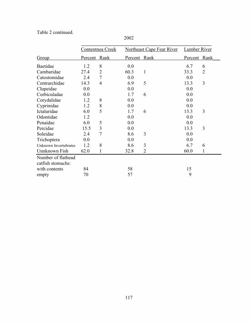
117

Table 2 continued. 2002

Contentnea Creek Northeast Cape Fear River Lumber River

Group Percent Rank Percent Rank Percent Rank___

Baetidae 1.2 8 0.0 6.7 6 Cambaridae 27.4 2 60.3 1 33.3 2 Catostomidae 2.4 7 0.0 0.0 Centrarchidae 14.3 4 6.9 5 13.3 3 Clupeidae 0.0 0.0 0.0 Corbiculadae 0.0 1.7 6 0.0 Corydalidae 1.2 8 0.0 0.0 Cyprinidae 1.2 8 0.0 0.0 Ictaluridae 6.0 5 1.7 6 13.3 3 Odontidae 1.2 0.0 0.0 Penaidae 6.0 5 0.0 0.0 Percidae 15.5 3 0.0 13.3 3 Soleidae 2.4 7 8.6 3 0.0 Trichoptera 0.0 0.0 0.0 Unknown Invertebrates 1.2 8 8.6 3 6.7 6 Unnknown Fish 62.0 1 32.8 2 60.0 1 Number of flathead catfish stomachs: with contents 84 58 15 empty 70 57 9

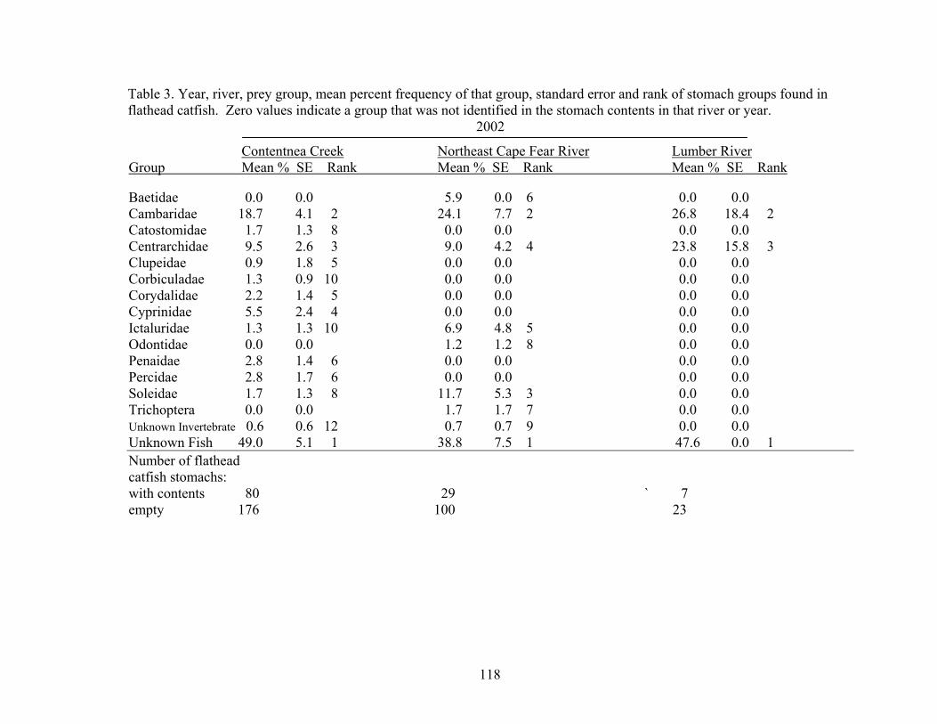
118

Table 3. Year, river, prey group, mean percent frequency of that group, standard error and rank of stomach groups found in flathead catfish. Zero values indicate a group that was not identified in the stomach contents in that river or year.

2002

Contentnea Creek Northeast Cape Fear River Lumber River Group Mean % SE Rank Mean % SE Rank Mean % SE Rank Baetidae 0.0 0.0 5.9 0.0 6 0.0 0.0 Cambaridae 18.7 4.1 2 24.1 7.7 2 26.8 18.4 2 Catostomidae 1.7 1.3 8 0.0 0.0 0.0 0.0 Centrarchidae 9.5 2.6 3 9.0 4.2 4 23.8 15.8 3 Clupeidae 0.9 1.8 5 0.0 0.0 0.0 0.0 Corbiculadae 1.3 0.9 10 0.0 0.0 0.0 0.0 Corydalidae 2.2 1.4 5 0.0 0.0 0.0 0.0 Cyprinidae 5.5 2.4 4 0.0 0.0 0.0 0.0 Ictaluridae 1.3 1.3 10 6.9 4.8 5 0.0 0.0 Odontidae 0.0 0.0 1.2 1.2 8 0.0 0.0 Penaidae 2.8 1.4 6 0.0 0.0 0.0 0.0 Percidae 2.8 1.7 6 0.0 0.0 0.0 0.0 Soleidae 1.7 1.3 8 11.7 5.3 3 0.0 0.0 Trichoptera 0.0 0.0 1.7 1.7 7 0.0 0.0 Unknown Invertebrate 0.6 0.6 12 0.7 0.7 9 0.0 0.0 Unknown Fish 49.0 5.1 1 38.8 7.5 1 47.6 0.0 1 Number of flathead catfish stomachs: with contents 80 29 ` 7 empty 176 100 23

119

Table 3 continued.

2002

Contentnea Creek Northeast Cape Fear River Lumber River Group Mean % SE Rank Mean % SE Rank Mean % SE Rank Baetidae 0.3 0.2 13 0.0 0.0 1.7 1.7 7 Cambaridae 19.3 3.9 2 53.4 6.1 1 42.8 9.9 1 Catostomidae 2.5 1.7 7 0.0 0.0 0.0 0.0 Centrarchidae 7.0 2.3 4 4.8 2.7 4 5.1 3.5 3 Clupeidae 0.0 0.0 0.0 0.0 0.0 0.0 Corbiculadae 0.0 0.0 0.4 0.4 7 0.0 0.0 Corydalidae 0.6 0.6 11 0.0 0.0 0.0 0.0 Cyprinidae 1.2 1.2 8 0.0 0.0 0.0 0.0 Ictaluridae 3.4 1.8 5 0.9 0.9 6 3.3 3.3 5 Odontidae 0.4 0.4 12 0.0 0.0 0.0 0.0 Penaidae 3.1 1.5 6 0.0 0.0 0.0 0.0 Percidae 9.1 2.8 3 0.0 0.0 4.3 3.4 4 Soleidae 0.7 0.6 10 4.6 2.2 5 0.0 0.0 Trichoptera 0.0 0.0 0.0 0.0 0.0 0.0 Unknown Invertebrate 1.2 1.2 8 7.5 3.3 3 1.9 1.9 6 Unknown Fish 51.5 4.9 1 28.5 5.7 2 38.7 10.1 2 Number of flathead catfish stomachs: with contents 84 58 ` 15 empty 74 57 9

120

Table 4. Year, river, prey group, total weight (g) of group in stomach contents, percentage of the total weight for all stomach contents, and rank (ascending order) of stomach items found in flathead catfish. Zero values indicate a group that was not identified in the stomach contents in that river or year.

2001

Contentnea Creek Northeast Cape Fear River Lumber River Group Total weight % Rank Total weight % Rank Total weight % Rank Baetidae 0.0 0.0 0.04 0.03 6 0.0 0.0 Cambaridae 23.6 4.0 4 34.3 27.7 2 0.5 12.1 3 Catostomidae 5.8 1.0 7 56.9 0.0 0.0 0.0 Centrarchidae 286.1 48.2 1 13.4 45.9 1 2.0 51.8 1 Clupeidae 16.7 2.8 5 0.0 0.0 0.0 0.0 Corbiculadae 0.8 0.1 10 0.0 0.0 0.0 0.0 Corydalidae 0.9 0.1 10 0.0 0.0 0.0 0.0 Cyprinidae 2.4 0.4 9 0.0 0.0 0.0 0.0 Ictaluridae 5.1 0.9 8 13.4 10.9 5 0.0 0.0 Odontidae 0.0 0.0 0.3 0.02 7 0.0 0.0 Penaidae 0.4 0.1 12 0.0 0.0 0.0 0.0 Percidae 170.9 28.8 2 0.0 0.0 0.0 0.0 Soleidae 6.8 1.2 6 6.8 5.5 5 0.0 0.0 Trichoptera 0.0 0.0 0.0 0.0 0.0 0.0 Unknown Invertebrate 0.01 0.0 0.01 0.01 8 0.0 0.0 Unknown Fish 74.0 12.5 3 12.4 10.0 4 1.4 36.1 2 All fish total 95.7 72.3 87.9 All invertebrate total 4.3 27.8 12.1 Number of flathead catfish stomachs: with contents 80 29 ` 7 empty 96 71 16

121

Table 4 continued.

2002

Contentnea Creek Northeast Cape Fear River Lumber River Group Total weight % Rank Total weight % Rank Total weight % Rank Baetidae 0.02 0.1 11 0.0 0.0 0.01 0.1 7 Cambaridae 38.1 10.1 3 114.2 52.4 1 18.5 14.6 4 Catostomidae 13.7 3.6 4 0.0 0.0 0.0 0.0 Centrarchidae 245.9 65.0 1 40.4 18.5 3 27.4 21.7 2 Clupeidae 0.0 0.0 0.0 0.0 0.0 0.0 Corbiculadae 0.0 0.0 5.2 2.4 0.0 0.0 Corydalidae 0.2 0.0 11 0.0 0.0 0.0 0.0 Cyprinidae 1.3 0.3 8 0.0 0.0 0.0 0.0 Ictaluridae 8.8 2.3 6 6.6 0.0 55.8 44.1 1 Odontidae 0.2 0.1 12 0.0 3.0 4 0.0 0.0 Penaidae 1.0 0.3 9 0.0 0.0 0.0 0.0 Percidae 12.8 3.4 5 0.0 0.0 0.5 0.4 5 Soleidae 2.5 0.7 7 3.5 1.6 6 0.0 0.0 Trichoptera 0.0 0.0 0.0 0.0 0.0 0.0 Unknown Invertebrate 0.8 0.2 10 1.2 0.5 7 0.2 0.1 6 Unknown Fish 53.4 14.1 2 46.9 21.5 2 24.1 19.1 3 All fish total 89.3 44.7 85.3 All invertebrate total 10.7 55.3 14.8 Number of flathead catfish stomachs: with contents 84 58 ` 15 empty 74 57 9

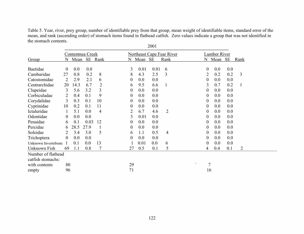
122

Table 5. Year, river, prey group, number of identifiable prey from that group, mean weight of identifiable items, standard error of the mean, and rank (ascending order) of stomach items found in flathead catfish. Zero values indicate a group that was not identified in the stomach contents.

2001

Contentnea Creek Northeast Cape Fear River Lumber River Group N Mean SE Rank N Mean SE Rank N Mean SE Rank Baetidae 0 0.0 0.0 3 0.01 0.01 6 0 0.0 0.0 Cambaridae 27 0.8 0.2 8 8 4.3 2.5 3 2 0.2 0.2 3 Catostomidae 2 2.9 2.1 6 0 0.0 0.0 0 0.0 0.0 Centrarchidae 20 14.3 6.7 2 6 9.5 6.6 1 3 0.7 0.2 1 Clupeidae 3 5.6 3.2 3 0 0.0 0.0 0 0.0 0.0 Corbiculadae 2 0.4 0.1 9 0 0.0 0.0 0 0.0 0.0 Corydalidae 3 0.3 0.1 10 0 0.0 0.0 0 0.0 0.0 Cyprinidae 10 0.2 0.1 11 0 0.0 0.0 0 0.0 0.0 Ictaluridae 1 5.1 0.0 4 2 6.7 4.6 2 0 0.0 0.0 Odontidae 0 0.0 0.0 3 0.01 0.0 0 0.0 0.0 Penaidae 6 0.1 0.03 12 0 0.0 0.0 0 0.0 0.0 Percidae 6 28.5 27.9 1 0 0.0 0.0 0 0.0 0.0 Soleidae 2 3.4 3.0 5 6 1.1 0.5 4 0 0.0 0.0 Trichoptera 0 0.0 0.0 0 0.0 0.0 0 0.0 0.0 Unknown Invertebrate 1 0.1 0.0 13 1 0.01 0.0 6 0 0.0 0.0 Unknown Fish 69 1.1 0.8 7 27 0.5 0.1 5 4 0.4 0.1 2 Number of flathead catfish stomachs: with contents 80 29 ` 7 empty 96 71 16

123

Table 5 Continued.

2002

Contentnea Creek Northeast Cape Fear River Lumber River Group N Mean SE Rank N Mean SE Rank N Mean SE Rank Baetidae 1 0.02 . 11 0 0.0 0.0 1 0.01 . 7 Cambaridae 30 1.3 0.3 4 43 2.7 0.4 3 16 1.2 0.2 4 Catostomidae 4 3.4 1.7 2 0 0.0 0.0 0 0.0 0.0 Centrarchidae 17 14.5 7.3 1 5 8.1 3.8 1 4 6.9 0.2 2 Clupeidae 0 0.0 0.0 0 0.0 0.0 0 0.0 0.0 Corbiculadae 0 0.0 0.0 2 2.6 0.0 4 0 0.0 0.0 Corydalidae 1 0.2 . 0 0.0 0.0 0 0.0 0.0 Cyprinidae 1 1.3 . 4 0 0.0 0.0 0 0.0 0.0 Ictaluridae 5 1.8 0.7 3 1 6.6 . 2 2 27.9 27.9 1 Odontidae 1 0.2 . 10 0 0.0 0.0 0 0.0 0.0 Penaidae 5 0.2 0.03 10 0 0.0 0.0 0 0.0 0.0 Percidae 42 0.3 0.03 9 0 0.0 0.0 4 0.1 0.04 5 Soleidae 2 1.2 0.9 6 5 0.7 0.5 6 0 0.0 0.0 Trichoptera 0 0.0 0.0 0 0 0.0 0.0 0 0.0 0.0 Unknown Invertebrate 1 0.8 . 7 5 0.2 0.2 7 2 0.1 0.0 6 Unknown Fish 110 0.5 0.2 8 24 2.0 0.1 5 15 1.6 1.2 3 Number of flathead catfish stomachs: with contents 84 58 ` 15 empty 74 57 9

124

Table 6. Sample year, sample month, river, sample size, TL (mm) ± SE, Weight (g) ± SE, and stomach fullness ± SE of flathead catfish with stomach contents. Year Month River N TL (mm) ± SE Wt (g) ± SE Fullness ± SE

2001 July Contentnea 15 492 ± 45 1,827 ± 432 0.67 ± 0.33 August Contentnea 53 455 ± 25 1,636 ± 305 0.33 ± 0.08 September Contentnea 13 428 ± 61 1,785 ± 960 0.73 ± 0.35 2002 May Contentnea 19 498 ± 27 1,688 ± 295 0.20 ± 0.05 June Contentnea 23 512 ± 38 2,164 ± 446 0.44 ± 0.17 July Contentnea 24 438 ± 35 1,390 ± 366 0.27 ± 0.60 August Contentnea 11 301 ± 72 1,504 ± 621 0.30 ± 0.09 2001 July Lumber 2 572 ± 291 4,225 ± 4025 0.42 ± 0.40 August Lumber 2 563 ± 117 2,225 ± 1275 0.95 ± 0.72 2002 April Lumber 9 654 ± 50 3,823 ± 882 0.27 ± 0.15 May Lumber 5 493 ± 67 1,552 ± 452 2.20 ± 1.60 June Lumber 1 867 ± 0 7,550 ± 0 0.001 ± 0 July Lumber 0 August Lumber 1 447 ± 0 910 ± 0 0.95 ± 0 2001 July NE Cape Fear 10 407 ± 53 1,205 ± 547 2.40 ± 0.76 August NE Cape Fear 12 409 ± 46 1,237 ± 476 3.00 ± 1.32 September NE Cape Fear 2 413 ± 139 1,083 ± 867 3.70 ± 3.1 October NE Cape Fear 5 420 ± 76 1,029 ± 647 0.47 ± 0.4 2002 April NE Cape Fear 8 555 ± 88 4,681 ± 3344 1.50 ± 0.53 May NE Cape Fear 15 381 ± 46 1,096 ± 390 3.80 ± 1.4 June NE Cape Fear 9 298 ± 40 444 ± 265 1.50 ± 1.0 July NE Cape Fear 5 449 ± 58 1,216 ± 473 0.28 ± 0.1 August NE Cape Fear 19 379 ± 40 989 ± 295 0.41 ± 0.13 September NE Cape Fear 5 239 ± 79 1,043 ± 88 0.18 ± 5

125

Figure Caption

Figure 1. Correlation between diet item size (mm) and flathead catfish (FHC) total length (mm) for Contentnea Creek and the Northeast Cape Fear River in 2001 and 2002. Correlation coefficient (R) and p values are shown.

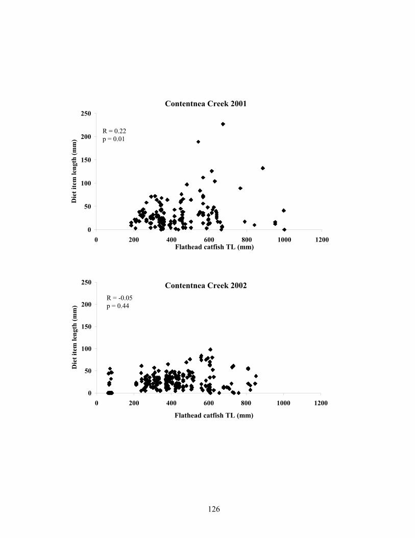
126

0

50

100

150

200

250

0 200 400 600 800 1000 1200Flathead catfish TL (mm)

Die

t ite

m le

ngth

(mm

)

0

50

100

150

200

250

0 200 400 600 800 1000 1200

Flathead catfish TL (mm)

Die

t ite

m le

ngth

(mm

)

R = 0.22 p = 0.01

Contentnea Creek 2001

Contentnea Creek 2002 R = -0.05 p = 0.44

127

0

50

100

150

200

250

0 200 400 600 800 1000 1200Flathead catfish TL (mm)

Die

t ite

m le

ngth

(mm

)

0

50

100

150

200

250

0 200 400 600 800 1000 1200

Flathead catfish TL (mm)

Die

t ite

m le

ngth

(mm

)

R = 0.15 p = 0.24

Northeast Cape Fear River 2001

Northeast Cape Fear River 2002

R = -0.045 p = 0.668

128

CHAPTER 5

MODELING THE EFFECTS OF AN INTRODUCED APEX PREDATOR

ON A COASTAL RIVERINE FISH COMMUNITY

129

Abstract

The flathead catfish, a carnivorous fish species native to most of the central interior

basin of North America, has been introduced into at least 13 U.S. states and one Canadian

province. Concurrent declines in abundance of native fishes have been reported in areas

where flathead catfish have been introduced. To evaluate the impact of this invasive species

on the native fish community, I developed an ecosystem simulation model (including

flathead catfish) based on empirical data collected for a North Carolina coastal river. Model

results suggest that flathead catfish suppress native fish community biomass by 5-50%

through both predatory and competitive interactions. However, these reductions could be

mitigated through sustained exploitation of flathead catfish by recreational or commercial

fishers at levels equivalent to those for native flathead catfish populations (annual

exploitation = 6-25%). These findings demonstrate the potential for using directed harvest

of an invasive species to assist in restoring native ecosystems and contribute to the growing

global demand for fish products as a human food source.

Introduction

The introduction and establishment of non-native species is a widespread and poorly

understood global phenomenon. While most species introductions fail or persist unnoticed

(Williamson 1996), some lead to declines in the abundance or diversity of native species–

and occasionally cascading negative ecosystem level effects which impact human

populations (Folkerts 1997). The annual economic impact of the 50,000 nonnative species

that have been introduced into the United States is about U.S. $137 billion (Pimentel et al.

2000)– an amount 13 times larger than the 2003 budget for the Department of Interior, the

130

primary United States governmental agency charged with conservation and management

(U.S. Department of the Interior, Office of the Budget Director). This cost does not include

the impacts of species that have been translocated within the United States and their potential

effect (Pimentel et al. 2000).

Generalizations describing the biotic and abiotic characteristics that regulate the

success or failure of an invasive species have been derived based on field, experimental, and

theoretical studies (Elton 1958; Williamson 1996), and the resulting body of literature

describing invasive species is immense. Invading species encounter environmental (e.g.,

suitable habitat), biotic (e.g., competition), and demographic (e.g., reproductive traits)

resistance that must be overcome to establish a self-sustaining population (Moyle and Light

1996a). Failure in any one of these areas usually leads to the invasion failing (as most do).

However, in situations where invasive species have been purposefully introduced for food or

recreation, humans have often selected species with desirable (to humans) physical traits

(e.g., large size, palatable flesh) and introduced these species repeatedly into ecosystems that

are more vulnerable to invasion (e.g., highly disturbed or degraded systems) (Moyle and

Light 1996b). This human intervention increases the likelihood of a successful invasion by

circumventing many of the naturally existing invasion obstacles.

While often not as captivating as introductions from regions outside of the United

States, translocations of nonnative species within the country have had dramatic impacts on

aquatic ecosystems. Community compositions in both coastal and inland aquatic ecosystems

in the United States have been widely and severely altered by species introductions. For

example, two endemic Atlantic slope fishes, striped bass Morone saxatilis and American

shad Alosa sapidissima, were both introduced and established along the United States west

131

coast in the 19th century, and largemouth bass Micropterus salmoides, with a native range

primarily in the Mississippi River valley and southern Atlantic slope, is now found

throughout North America and around the world (Li and Moyle 1993; Nielsen 1993). It is

clear that fish faunas across the continental United States are becoming more similar through

widespread introductions of fish species intended to enhance food and sport fisheries (Rahel

2000). However the effects of these species introductions are not fully understood and are

rarely considered until after the introduced species has become established, greatly limiting

management options.

The flathead catfish Pylodictis olivaris is a large piscivorous catfish native to most of

the interior US throughout the Rio Grande, Mississippi, and Mobile River drainages (Smith-

Vaniz 1968; Jenkins and Burkhead 1994). Flathead catfish have been legally and illegally

introduced into at least 13 United States (primarily along the Atlantic slope) and one

Canadian province (Jackson 1999) usually in an effort to establish recreational fisheries.

Within 15 years following their introduction into North Carolina (only documented

introduction is of 11 individuals), flathead catfish have expanded to cover a 200-km reach of

the Cape Fear River and have emerged as the dominant predator within the drainage basin

(Guier et al. 1981).

Flathead catfish are widely prized throughout their native range as a trophy sportfish

due to their large size (current world angling record 56.4 kg), fighting ability when hooked,

and highly palatable flesh. These qualities support recreational and commercial fisheries

throughout their native range and developing fisheries throughout their introduced range

(Quinn 1993; Jackson 1999; Travnicheck and Clemmons 1999). Unlike most other catfishes,

flathead catfish are obligate carnivores and primarily piscivorous, and given their potential to

132

reach large sizes, their feeding patterns have been widely studied to discern their interactions

with other fish species. Swingle (1967) documented that flathead catfish >254-mm total

length “may compete with fishermen for fish of harvestable size” in ponds. Results from

similar diet studies, as well as widespread concern over declining populations of native fishes

following flathead catfish introduction, have compelled study of flathead catfish food habits

in their introduced range (Guier et al. 1981; Ashley and Buff 1987; Quinn 1987; Thomas

1995). These studies generally document a decline in native sportfish populations (likely via

predation) following introduction of flathead catfish. The species affected are usually native

centrarchids and ictalurids, but other natives including the federally endangered razorback

sucker Xyrauchen texanus in the San Pedro River, Arizona, are thought to be threatened by

flathead catfish introduction (Marsh and Brooks 1989).

In this paper, I develop an ecosystem model including flathead catfish in a North

Carolina coastal plain river based on empirical data from the system. Given the seemingly ever

increasing global demand for fish products, the ability of humans to alter aquatic ecosystems

through intensive fishing efforts (Jackson et al. 2001), the popularity of flathead catfish as a food

fish in its native range (Jackson 1999), and the large recreational and commercial fisheries

interest in North Carolina (National Marine Fisheries Service 2001), flathead catfish may be an

excellent candidate species to promote for more intensive harvest. Flathead catfish harvest

would provide a desired food product and may also help restore native ecosystems by reducing

the biomass of an invasive species. Here I examine how manipulating exploitation rates of

flathead catfish affects their abundance and ecological role in structuring the native fish

community. These simulations may prove useful in management scenarios for established and

133

newly introduced populations of flathead catfish and for understanding the ecological

consequences of this and other introduced species.

Methods

Model Design

I developed an ecosystem simulation model based on Contentnea Creek (35°20’03”N

77°22’73”W), a large tributary of the Neuse River in eastern North Carolina, using an

Ecopath and Ecosim framework (Walters et al. 1997; Christianson et al. 2000). The initial

model is a static mass balance of the production and losses of the biomass for each

component of an ecosystem. Balance is achieved when production and immigration is equal

to predatory losses, nonpredatory mortality, harvest, and emigration. Because all variables

are linked within a food web, changes in one variable are expressed as changes in other

(often many) components of the web. Flow and linkages are established among different

components of the food web model. A second model (Ecosim) simulates changes in the

initial “balanced” steady-state of the food web (the Ecopath model) with altered exploitation

rates, species interactions, environmental changes, or a combination of factors. Similar

models have been used to examine the linkages between primary production, fish production,

and fishery exploitation in marine and freshwater systems and also the linkage between plant

community biomass, herbivore density, and predator density in the Canadian arctic (Krebs et

al. 2003). Explicit details of the modeling approach are published elsewhere (Walters et al.

1997; Christianson et al. 2000).

My model was developed incorporating empirical data from a multi-investigator

project evaluating the interaction between flathead catfish and native fish communities in

North Carolina coastal plain rivers (NCWRC report). Most field sampling efforts occurred

134

during spring through early fall of 2000-2003 when warm water temperatures were

conducive to sampling both introduced and native fishes (Chapter 3). My model was

composed of 12 functional groups: nine fish, one invertebrate, one plankton, and one detritus

(Table 1). Fish were grouped based on similar morphometric, feeding, and life-history

functional attributes (Table 1). For example, flathead catfish were placed in an “exotic

piscivore” group while all darters (Percina and Etheostoma spp.) and minnows (Notropis

spp.) were placed in a single “omnivore-collector” group.

Model initialization required estimates for each functional group of habitat area used,

biomass (B), production:biomass ratio (P:B), consumption:biomass ratio (Q:B), diet

information, and biomass harvested. As much as possible, this information was derived

empirically for each functional group. For example, estimates of instantaneous mortality (Z)

were obtained for flathead catfish using catch-curve analysis (NCWRC report), while

mortality estimates for other functional groups were calculated by dividing the annual

production for each functional group by its biomass. Biomass for each fish functional group

was estimated by first calculating the abundance for each individual species using a three-

pass removal method (Seber 1982). Individual fish weights were measured in the field, and

the average weight was assigned to each species in the functional group. A weighted average

(weighted by species abundance) was then used to calculate the mean biomass for that entire

functional group. Capture histories from the removals were pooled for each functional group

to develop a group-wide capture-probability to allow abundance estimation for the species

where removal estimates were not possible (Appendix 1). Contentnea Creek supports spring

runs of anadromous shad (Alosa spp.) and striped bass, which occurred prior to my sampling.

For this modeling effort, I only considered the sizes and densities of each genus collected

135

during my sampling period. Thus, only juvenile alosids (a prey item) and resident striped

bass (a predator found in low numbers, which does not return to the marine environment in a

given year) are included in my model.

Removal population estimates were conducted in late spring and early fall, thus

approximate annual P:B ratio values could be calculated by subtracting the biomass of a

functional group in the fall from that group’s biomass in the spring and dividing by the spring

biomass. Q:B ratios for each species were calculated using the online estimator available

through Fishbase (www.fishbase.org), which is based on equations provided in Pauly (1986)

and Palomares and Pauly (1989). An average Q:B for each functional group was then

calculated using a weighted mean (by abundance of each individual species). Diet matrices

were developed from empirical diet samples conducted in conjunction with this study (for

flathead catfish) or from published reports (Appendix 2).

Exploitation rates for all fish species in Contentnea Creek are relatively low,

primarily due to the remote location and limited stream access. Harvest occurs for several

species included in my model, primarily native Lepomis spp., Micropterus spp., striped bass,

and flathead catfish. I used an estimated annual biomass exploitation level (u) for flathead

catfish for modeling efforts of 4% based on harvest rates of a group of fish radio-tagged as

part of another aspect of my study (W. E. Pine, unpublished data). Because of uncertainty

associated with this exploitation rate, I simulated a wide range of exploitation rates that cover

most potential exploitation levels for flathead catfish in this and other systems. Exploitation

estimates for other species were derived from the literature. Recreational fisheries for

flathead catfish in native rivers are estimated to have annual exploitation rates of 25% or

more (Vince Travnichek, Missouri Department of Conservation and Natural Resources,

136

Columbia, Missouri, personal communication) and in introduced populations between 14 and

25% (Quinn 1993). Combined with commercial fisheries, total exploitation rates could be

higher. All model parameters are provided in Appendix 2.

Model Application and Scenarios

Following the introduction of an invasive species, resource management agencies

frequently focus their efforts on eradication options for the invader. However, invasive

species may become well established before management actions occur, and complete

removal is rarely a viable option. Instead, resource management agencies may become

interested in the impacts of the invasive species on native species and how manipulation of

invasive species abundance might impact native populations. Because many fish species

(including flathead catfish) represent a marketable food product, and fisheries management

agencies, commercial fishing interests, and recreational anglers have a history of

manipulating and exploiting fish populations, I used this model to evaluate how native fish

communities would respond to varying reductions in flathead catfish populations via

intensive exploitation. I evaluated three different model scenarios (1) changes in the native

fish community under a modeling scenario which emulates the original introduction of

flathead catfish in a coastal North Carolina river, (2) evaluation of ecosystem response to

high levels of flathead catfish exploitation in an attempt to extirpate flathead catfish from a

coastal river, and (3) native fish response to sustained exploitation of flathead catfish across a

range of exploitation levels similar to those found for native populations of flathead catfish.

Historical Invasion Analysis

I used historical information on the introduction of flathead catfish in North Carolina

to evaluate the predicted response and rate of change by the native fish community to

137

flathead introduction. The only documented release of flathead catfish into North Carolina

waters was a single release of 11 individuals with a total weight of 107 kg into the Cape Fear

River, a large North Carolina coastal plain river about 75 km southeast of Contentnea Creek

(Guier et al. 1981). The source or date of the flathead catfish introduction in Contentnea

Creek is not known. As a general assessment of my overall modeling approach, I evaluated

how early reports of the rapid growth in the flathead catfish population and subsequent

changes within the native fish community compare to the predictions of my model. Because

this model is based on an ecosystem that already contains flathead catfish, the invasion

scenario was developed differently than the scenarios below. First, flathead catfish

exploitation was simulated to be very high, in effect removing flathead catfish from the

system. The ecosystem without flathead catfish was then allowed to reach equilibrium. This

equilibrium was considered to simulate the ecosystem in the absence of flathead catfish.

Flathead catfish were then added to the ecosystem at the same population biomass as the

Cape Fear River introduction, and the ecosystem response was measured from this point.

Sustained Fishing Pressure

I simulated the population level responses of the native fish groups to a variety of

flathead catfish exploitation levels. The simulated exploitation levels (u) of 6 and 25%

cover the range of reported flathead catfish exploitation in native and introduced populations.

Each of these exploitation levels were sustained for 10 years. The resiliency of both flathead

catfish and native fish populations to increased flathead catfish exploitation was then

examined by reducing exploitation to current levels and monitoring ecosystem response.

I then evaluated a “maintenance control” option where flathead catfish exploitation

oscillates between a 5-year high exploitation period (u = 25%) and a reduced exploitation

138

period (u = 6%) for 5 years. Again, simulated exploitation levels mimic actual reported rates

for native populations of flathead catfish. These reported rates are exclusively from

recreational fishing although commercial fishing could also have the same or greater impact.

Flathead Catfish Eradication

Management agencies often consider efforts to remove invasive species to help restore

ecosystems to their native condition. I examined ecosystem response to an effort to eliminate

flathead catfish by simulating an intensive removal effort via simulated exploitation of 33 and

54% (10 and 20 times current levels) sustained for 10 years. Intensive exploitation was then

stopped, and ecosystem response was monitored for 10 years as above. Additionally, long-term

resiliency to intensive exploitation was evaluated by conducting the same eradication

simulations, but monitoring the ecosystem for longer time periods, 50 years for the u= 33% and

100 years for the u= 54% scenario. These exploitation rates could be achieved through resource

agency personnel targeting flathead catfish for removal through scientific sampling in

conjunction with commercial and recreational fishing efforts.

Results

Invasion

My invasion simulation was initiated with the same “introduction” biomass as the

original flathead catfish release into the Cape Fear River. This simulation resulted in

declines of about 30% in the anadromous shad and native insectivore groups and about a

50% decline in the anadromous and native piscivore groups (Figure 1). Other groups

declined by about 5-15% with the exception of native detritivores, which increased by about

30% (Figure 1). In this invasion scenario, flathead catfish were predicted to become the

dominant apex piscivore by population biomass in less than 50 years.

139

Sustained Fishing Pressure

Currently exploitation for flathead catfish in Contentnea Creek is low, about 4% per

year. My model predicted that reducing flathead catfish biomass via increasing exploitation

rates to 6% would lead to only a 2-3% increase in most native fish groups (Figure 2). As

exploitation rate increases, flathead catfish biomass declines, and native fish biomass

increases. Increases in population biomass of about 25-75% were predicted for native

piscivores, native insectivores, anadromous piscivores, and estuarine species in less than 10

years following an increase in flathead catfish exploitation to either 25 or 33% (Figure 2).

Other native fish groups including omnivores and omnivore collectors also showed

population biomass increases of 2-10%. If higher fishing pressure is not sustained,

population biomass of all functional groups are predicted to return to pre-increased fishing

levels in less than 10 years.

Eradication Efforts

Simulated flathead catfish exploitation levels of more than 33% were not sustainable, and

at this level flathead catfish were nearly eliminated from the system by harvest. At 33%

exploitation, flathead catfish biomass was reduced by about 90% within 10 years (Figure 3). A

larger increase in exploitation (54% exploitation) reduced flathead catfish biomass by about 95%

within 5 years nearly extirpating flathead catfish from the system for at least 15 years. This

reduction in flathead catfish biomass resulted in the biomass doubling for native and anadromous

piscivores, an approximate 50% increase for native insectivores, anadromous shad, and estuarine

species, and biomass increases of 5-15% for native omnivores and omnivore-collectors.

140

Resiliency to Exploitation

My simulations demonstrate flathead catfish resiliency to exploitation. If exploitation

ranges from 6 - 33% for a period of 10 years and then is reduced to current levels (about 4%),

flathead catfish populations will return to their initial biomass within 5-50 years, and

subsequently reduce native fish populations to pre-exploitation levels (Figures 2, 4). Under a

modeling scenario of very high exploitation levels (54% exploitation) sustained for 10 years

flathead catfish populations were predicted to crash (0.01% of original biomass), yet recover

from this intense harvest and return to original levels in about 80 years (Figure 4).

The maintenance control management scenario (alternating 5-year periods of high

and low exploitation) dampened the observed resiliency to decreased fishing pressure and

maintained relatively high positive increases in native fish biomass (Figure 5). As previously

predicted, the greatest change in native fish abundance came when flathead catfish

abundance was lowest (u = 25%). However, even when fishing pressure was reduced (u

=6%) following five years of high fishing pressure, biomass of most native fish was still

much higher than it would have been at the low fishing rate alone. Average biomass

response during the maintenance control simulations for recreationally important species was

highest for native and anadromous piscivores (approximately 70% increase each), followed

by native insectivores and anadromous shad (approximately 30% increase each). Average

flathead catfish biomass reductions were approximately 70%.

Discussion

The results of this modeling exercise suggest that reduction of flathead catfish

biomass via exploitation may allow an increase in population biomass of a variety of native

fish groups. Native apex predators in my model (native and anadromous piscivore groups)

141

showed the greatest response to the initial introduction and reductions in flathead catfish

populations, likely because of interspecific competition with flathead catfish for available

food resources. Native insectivores also showed strong positive increases in biomass

following increased exploitation. Native omnivores and the omnivore-collector group were

both predicted to increase following reductions in flathead biomass. Although neither of

these groups competes directly with adult flathead catfish for food resources, they are both

comprised of flathead catfish prey items– thus reduction in flathead catfish biomass reduces

total mortality of these groups, increasing biomass. The native-omnivore collector group is

comprised of native darter and minnow species, groups that are particularly sensitive to

anthropogenic changes in aquatic environments. The additional survival pressure on these

groups induced by an invasive predator species could be particularly detrimental in an

already stressed physical environment.

Two groups showed unexpected results associated with declines in flathead catfish

biomass. The estuarine group was composed primarily of hogchokers Trinctes maculatus,

and the unique body shape of this benthic flatfish was easily identified in the flathead catfish

diet samples. This may have led to an over-representation of hogchokers in the model diet

matrix for flathead catfish, and coupled with their natural low biomass in the system, their

response to reductions in flathead catfish biomass may be exaggerated.

Native detritivores generally declined in biomass as exploitation rates increased for

flathead catfish. The mechanism for these declines may be greater predation mortality on

this group from the native and anadromous piscivore groups that were released from

competition with flathead catfish. My native detritivores group included several redhorse

(Moxostoma spp.) species, a group which corollary declines in abundance have been found in

142

areas where flathead catfish have been introduced (Bart et al. 1994). Conversely, Guier et al.

(1981) observed an increase in percent occurrence of Moxostoma sp. in the Cape Fear River

following flathead catfish introduction, similar to the results of my modeling for the native

detritivore group. These conflicting findings are not unexpected given the varying impacts

invasive species can have on different ecosystems (Chapter 6). This model was developed

for a very similar system as Guier et al. (1981) thus similarity between the model predictions

and empirical observations are expected. An Ecopath model for the systems examined by

Bart et al. (1984) may be similar to those systems.

Restoration efforts for anadromous shad are currently underway in several rivers

along the Atlantic slope of the United States (Beasley and Hightower 2000). My model

included a juvenile anadromous shad component from my summer sampling of these fish

before they outmigrated to the ocean. The predicted increase in biomass for anadromous

shad as flathead catfish exploitation increased is particularly important to these restoration

efforts. In many fish species growth and survival during early life can affect adult fish

abundance (Houde 1987). Decreasing mortality at early life stages (such as the juveniles)

can potentially have large impacts on adult abundance. Resource managers should consider

increased juvenile and adult predation mortality from invasive predators such as flathead

catfish in designing restoration programs for anadromous shad species across the Atlantic

slope.

Complete elimination of flathead catfish is likely difficult from Contentnea Creek or

any coastal river where flathead catfish have become established. I documented flathead

catfish migration from Contentnea Creek throughout most of the Neuse River (NCWRC

Final Report). Because of this movement, the flathead catfish population is continuous

143

throughout the Neuse River basin instead of smaller discrete population units making

erradication options unrealistic. Aquatic plant managers are accustomed to dealing with

similar issues in designing control options for invasive aquatic plant species where efforts are

directed at maintaining the population of the invasive species at the lowest feasible levels

rather than complete eradication (Pieterse and Murphy 1990). By using maintenance control

techniques to keep populations at low densities, less time and financial resources are actually

expended by continuously harvesting populations, rather than by allowing population to

expand to large levels, and then attempting to reduce them. My maintenance control

simulations clearly demonstrate that this approach is possible with invasive flathead catfish.

In fact, the average population response for each native species group in the maintenance

control scenario (Figure 3) was at least twice as large as it would be from sustained harvest at

the “low” level (6%) (Figure 2).

Apex predators are often the most successful invasive species (Moyle and Light 1996

a, b). This conclusion is based on theory and observations that prey species are usually

highly vulnerable to the predation style of the newly introduced predator (Moyle and Light

1996 a). In my model, the groups most strongly affected by changes in flathead catfish

biomass are not species that are likely to be heavily preyed upon by flathead catfish (native

and anadromous piscivores), but instead are groups competing with flathead catfish for

available prey resources (primarily native insectivores). Coastal plain rivers in North

Carolina are anthropogenically disturbed (Benniger and Wells 1993; Glasgow and

Burkholder 2000) and relatively unproductive with low biomass of native fish species.

Because of this low productivity in a disturbed environment, competition for already limited

144

available prey resources with an introduced predator dampens native and anadromous

piscivore abundance.

The resiliency of flathead catfish populations to fishing pressure is largely a function

of the absence of any natural predator of this species. While several native piscivores in

Contentnea Creek are also found in the native range of flathead catfish, and these native

predators likely feed on juvenile flathead catfish, this predation pressure is not intensive

enough to suppress flathead catfish populations. This is similar to the cane toad Bufo

marinus invasion in Australia where population densities of cane toads are often much higher

in Australia than in the native South American habitats (Lamp and De Leao 1998). This

difference in population density between the two continents is primarily a function of higher

adult survival in Australia due to a lack of cane toad predators, pathogens, and parasites.

Moyle and Light (1996a) concluded that among environmental, biotic, and

demographic factors determining invasion success, environmental factors were the most

important, yet overall invasion success depends on the interaction of all three. Contentnea

Creek and the larger Neuse River watershed have been broadly affected by anthropogenic

and natural disturbance including flow regime alterations, poor land use practices, nutrient

enrichment and hurricanes (Cahoon et al. 1999; Paerl et al. 2001). All of these factors may

combine to lessen the invasion resistance of the native fish community. From an

ecologically detrimental invasive species perspective, flathead catfish represent the ideal

aquatic invader due to its predatory nature, broad habitat use (small and large lentic and lotic

systems), and appealing sporting characteristics to human users who have fostered their

introduction into new areas. However, while these traits may lend the species to successful

145

introducton and establishment in a wide variety of systems, they make the management of

this invasive species much more difficult.

Management Implications

My modeling results have shown that moderate, sustained levels of flathead catfish

exploitation may release native fish groups from predation by and competition with flathead

catfish. This finding is important for resource managers involved in restoring native fish

populations in areas where flathead catfish have been introduced. Management agencies

could promote harvest of flathead catfish populations by offering a bounty or subsidy system

to commercial fishers in an effort to establish an interest in harvesting this species (by

guaranteeing an attractive price) and simultaneously developing a market for the fish

product. Increasing the size and intensity of the recreational fishery is an equally important

aspect of any effort to reduce flathead catfish biomass and provide sustained fishing pressure.

Schramm et al. (1999) found that Mississippi catfish anglers preferred to fish in rivers and

streams and that anglers found it very important to “keep a lot of fish” leading those authors

to note that “…increased fishing effort and high harvest could deplete these [catfish]

resources.”

I found that flathead catfish exploitation rates in native systems (25%) would be more

than adequate to provide a large (>30%) increase in most native fish groups. However, this

level of exploitation would not likely be sustainable in the rivers I studied, leading to

overexploitation of the flathead catfish population—and subsequent declines in catch rates

and subsequently a loss of participants in the fishery. Given the resiliency of flathead catfish

populations to exploitation, the predicted benefits to native fish groups are only achievable if

flathead catfish fishing pressure is sustained to some degree. Declines in exploitation would

146

allow flathead catfish populations to rebound, subsequently losing the gains realized in the

native fish communities while flathead catfish populations were suppressed.

Although my simulations suggest that reducing flathead catfish biomass by increasing

exploitation rate could release most native fish groups from competition and predation

pressures leading to increases in biomass, there are several issues that should be considered

in evaluating these results. I examined changes in population biomass of a variety of fish

groups in response to exploitation of flathead catfish, which resulted in subsequent changes

in other components of the ecosystem through changes in predation mortality or resource

competition with other groups. However, size structure of individuals within each of these

groups is also likely to change, not just population biomass. For example, flathead catfish

exploitation may reduce the number of large individuals in the population, restructuring the

population to be dominated by smaller individuals. These smaller individuals may have

greater physiological energetic demands than the larger individuals that were removed from

the population. Increasing abundance of smaller flathead catfish could result in equal or

greater predation pressure on the native fish groups by the exploited flathead catfish

population, than by the unexploited population.

My modeling efforts also assume constant recruitment of all fish species. Allen and

Pine (2000) showed that changes in population biomass from altering exploitation rates could

be masked by variable recruitment in 3 or 5-year study periods for largemouth bass and white

crappie Pomoxis annularis. Recruitment variability is common in nearly all fish species,

thus changes in biomass for any species may be expedited (in years following low

recruitment) or delayed (in years following high recruitment). My manipulation of flathead

catfish biomass by altering mortality rates also alters total mortality of all other species in the

147

food web by changing predation mortality and competition. Thus, variable recruitment could

change the rate at which various components of the ecosystem respond to flathead catfish

exploitation.

My model was developed from information collected from an ecosystem that may

have already been altered by the invasion of flathead catfish. The current fish assemblage in

Contentnea Creek may suffer from the “ghost of predation past” (i.e., the ecosystem impact

resulting from predation pressure that occurred in the past remains evident today) such that

any potential impact to native species by the exotic was likely prior to this study. It is

possible that flathead catfish have extirpated species from Contentnea Creek or reduced

population levels below detectable levels. These species would obviously not be included in

my model and the interaction between species which no longer exist and other components of

the ecosystem cannot be evaluated. My model is based on the current conditions within the

ecosystem including impacts of flathead catfish. By manipulating flathead catfish biomass

and examining the population release in the native community based on current conditions, I

am not basing my predictions on uncertain estimates of past conditions.

Modeling exercises and empirical data both include error and many models may be

unreliable for quantitative predictions (Johnson 1995). Models such as the one used here are

useful for examining trends in ecosystem dynamics and providing insight into the cascading

effects of an invasive species on coastal riverine ecosystems. Given the impossibility of

controlled, replicated field studies involving invasive species a modeling method such as this

is ecologically the safest approach to elucidate species interactions.

My simulation results suggesting positive responses in native fish biomass following

flathead catfish harvest could be considered as a part of a broader ecosystem restoration

148

effort to mitigate the variety of anthropogenic ecosystem alterations in coastal rivers. While

many aspects of aquatic ecosystem restoration remain in an experimental phase (Lenihan et

al. 1999), our ability to harvest fish populations is well established, and directed harvest

toward flathead catfish may represent a conceptually simple, but important step in helping

restore native ecosystems.

149

References

Allen M. S., and W. E. Pine, III. 2000. Detecting fish population responses to a minimum length limit: effects of variable recruitment and duration of evaluation. North American Journal of Fisheries Management 20:672-682.

Ashley, K. W., and B. Buff. 1987. Food habits of flathead catfish in the Cape Fear River,

North Carolina. Proceedings of the Annual Conference Southeastern Association of Fish and Wildlife Agenices 41:93-99.

Bart, H. L., M. S. Taylor, J. T. Harbaugh, J. W. Evans, S. L. Schleiger, and W. Clark.

1994. New distribution records of Gulf Slope drainage fishes in the Ocmulgee River system, Georgia. Southeastern Fishes Council Proceedings. 30:4-9.

Beasley, C. A., and J. E. Hightower. 2000. Effects of a low-head dam on the distribution and

characteristics of spawning habitat used by striped bass and American shad. Transactions of the American Fisheries Society 129:1316-1330.

Benniger, L. K., and J. T. Wells. 1993. Sources of sediment to the Neuse River estuary, North

Carolina. Marine Chemistry 43:127-156. Cahoon, L. B., J. A. Mikucki, and M. A. Mallin. 1999. Nitrogen and phosphorus imports to

the Cape Fear and Neuse River basins to support intensive livestock production. Environmental Science and Technology 33:410-415.

Christiensen V., C. J. Walters, and D. Pauly. 2000. Ecopath with Ecosim: a user’s guide.

Vancouver: Fisheries Centre, University of British Columbia Research Report Series. Vancouver.

Davies, J. H. 1981. Food habits of largemouth bass in two coastal streams of North

Carolina. Pages 346-350 in L. A. Krumholz, editor. The warmwater streams symposium. American Fisheries Society Southern Division, Bethesda, Maryland.

Elton, C. S. 2000. The ecology of invasions of plants and animals. University of Chicago Press,

Chicago, Illinois. Folkerts, G. W. 1999. State and fate of the world’s aquatic fauna. Pages 1-16 in G. W.

Benz and D. E. Collins, editors. Aquatic fauna in peril: the southeastern perspective. The Southeastern Aquatic Research Institute Special Publication Number 1. Lenz Design and Communications, Inc., Decatur, Georgia.

Glasgow, H. B., and J. J. Burkholder. 2000. Water quality trends and management

implications from a five-year study of a eutrophic estuary. Ecological Applications 10:1024-1046.

150

Guier, R. C., L. E. Nichols, and R. T. Rachels. 1981. Biological investigation of flathead catfish in the Cape Fear River. Proceedings of the Annual Conference Southeastern Association of Fish and Wildlife Agencies 35:607-621.

Houde, E. D. 1987. Fish early life dynamics and recruitment variability. Pages 17-29 in R. D.

Hoyt, editor. 10th annual larval fish conference. American Fisheries Society, Symposium 2. Bethesda, Maryland.

Jackson, D. C. 1999. Flathead catfish: biology and management. Pages 23-36

in E. R. Irwin, W. A. Hubert, C. F. Rabini, H. L. Schramm, Jr., and T. Coon, editors. Catfish 2000: proceedings of the international ictalurid symposium. American Fisheries Society, Symposium 24, Bethesda, Maryland.

Jackson, J. B. C., M. X. Kirby, W. H. Berger, K. A. Bjorndal, L. W. Botsford, B. J.

Bourque, R. H. Bradbury, R. Cooke, J. Erlandson, J. A. Estes, T. P. Hughes, S. Kidwell, C. B. Lange, H. S. Lenihan, J. M. Pandolfi, C. H. Peterson, R. S. Steneck, M. J. Tegner, R. R. Warner. 2001. Historical overfishing and the recent collapse of coastal ecosystems. Science 293:629-638.

Jenkins, R. E., and N. M. Burkhead. 1994. Freshwater fishes of Virginia. American

Fisheries Society, Bethesda, Maryland. Johnson, B. L. 1995. Applying computer simulation models as learning tools in fishery

management. North American Journal of Fisheries Management 15:736-747. Kitchell, J. F., S. P. Cox, C. J. Harvey, T. B. Johnson, D. M. Mason, K. K. Shoen, K.

Aydin, C. Bronte, M. Ebner, M. Hansen, M. Hoff, S. Schram, D. Schreiner, C. J. Walters. 2000. Sustainability of the Lake Superior fish community: interactions in a food web context. Ecosystems 3:545-560.

Krebs, C. J., K. Danell, A. Angerbjörn, J. A. Dominque Berteaux, K. A. Bråthen, Ö. Danell,

S. Erlinge, V. Fedorov, K. Fedga, J. Hjältén. G. Högstedt, I. S. Jóngdóttir, A. J. Kenney, N. Kjellén, T. Nordin, J. Roininen, M. Svensson, M. Tannerfeldt, and C. Wiklund. 2003. Terrestrial trophic dynamics in the Canadian Arctic. Canadian Journal of Zoology 81:827-843.

Lampo, M., and G. A. De Leo. 1998. The invasion ecology of the toad Bufo marinus:

from South America to Australia. Ecological Applications 8:388-396. Lenihan, H. S., F. Micheli, S. W. Shelton, C. H. Peterson. 1999. The influence of multiple

environmental stressors on susceptibility to parasites: An experimental determination with oysters. Limnology and Oceanography 44:910-924.

151

Li, H. W., and P. B. Moyle. 1993. Management of introduced fishes. Pages 287-308 in C. C. Kohler and W. A. Hubert, editors. Inland fisheries management in North America. American Fisheries Society, Bethesda, Maryland.

Marsh, P. C., and J. E. Brooks. 1989. Predation by ictalurid catfishes as a deterrent to

re-establishment of hatchery-reared razorback suckers. Southwestern Naturalist 34:188-195.

Moyle, P. B., and T. Light. 1996 A. Biological invasions of fresh water: empirical rules and

assembly theory. Biological Conservation 78:149-161. Moyle, P. B., and T. Light. 1996 B. Fish invasions in California: Do abiotic factors determine

success? Ecology 77:1666-1670. Neal, J. W., R. L. Noble, and J. A. Rice. 1999. Fish community response to hybrid striped

bass introduction in small warmwater impoundments. North American Journal of Fisheries Management 4:1044-1053.

Nielsen, L. A. 1993. History of inland fisheries management in North America. Pages 3-31 in

C. C. Kohler and W. A. Hubert, editors. Inland fisheries management in North America. American Fisheries Society, Bethesda, Maryland.

Palomares, M. L., and D. Pauly. 1989. A multiple regression model for predicting the

food consumption of marine fish populations. Australian Journal of Marine and Freshwater Research 40:259-273.

Paerl, H. W., J. D. Bales, L. W. Ausley, C. P. Buzzelli, L. B. Crowder, L. A. Eby, J.

M. Fear, M. Go, B. L. Peierls, T. L. Richardson, J. S. Ramus. 2001. Ecosystem impacts of three sequential hurricanes (Dennis, Floyd, and Irene) on the United States’ largest lagoonal estuary, Pamlico Sound, NC. Proceedings of the National Academy of Science 98:5655-5660.

Pauly, D. 1986. A simple method for estimating the food consumption of fish populations from

growth data and food conversion experiments. Fisheries Bulletin 84:827-839. Pieterse, A. H., and K. J. Murphy. 1990. Aquatic weeds- the ecology and management of

nuisance aquatic vegetation. Oxford University Press. Oxford, England. Pimentel, D., L. Lach, R. Zuniga, and D. Morrison. 2000. Environmental and economic cost

of nonindigenous species in the United States. BioScience 50:53-65. Quinn, S. P. 1987. Stomach contents of flathead catfish in the Flint River, Georgia.

Proceedings of the Annual Conference Southeastern Association of Fish and Wildlife Agencies 41:85-92.

152

Quinn, S. P. 1993. Description of a multiple use fishery for flathead catfish. North American Journal of Fisheries Management 13:594-599.

Rahel, F. J. 2000. Homogenization of fish faunas across the United States. Science 288:854-

856. Schramm, H. L., Jr., J. T. Forbes, D. A. Gill, and W. D. Hubbard. 1999. Fishing

environment preferences and attitudes toward overharvest: are catfish anglers unique? Pages 417-426 in E. R. Irwin, W. A. Hubert, C. F. Rabini, H. L. Schramm, Jr., and T. Coon, editors. Catfish 2000: proceedings of the international ictalurid symposium. American Fisheries Society, Symposium 24, Bethesda, Maryland.

Seber, G. S. 1982. The estimation of animal abundance and other parameters. Macmillan

Publishing, New York. Smith-Vaniz, W. F. 1968. Freshwater fishes of Alabama. Paragon Press. Montgomery,

Alabama. Swingle, H. S. 1967. Experiments with the flathead catfish (“Pylodictis olivaris”) in

ponds. Proceedings of the Annual Conference Southeastern Association of Game and Fish Commissioners. 18: 303-308.

Thomas, M. E. 1995. Monitoring the effects of introduced flathead catfish on

sport fish populations in the Altamaha River, Georgia. Proceedings of the Annual Conference Southeastern Association of Fish and Wildlife Agencies 47:531-538.

Walters, C. J., V. Christensen, D. Pauly. 1997. Structuring dynamic models of

exploited ecosystems from trophic mass-balance assessments. Reviews in Fish Biology and Fisheries 7:1-37.

Waters, T. F. 1977. Secondary production in inland waters. Advances in Ecological

Research 10:91-164. Williamson, M. 1996. Biological invasions. Chapman and Hall, London, England.

153

Table 1. Species composition of each functional group included in the Ecopath model Functional Grouping Species Name Exotic Piscivore Pylodictis olivaris, Flathead catfish Native Piscivore Pomoxis nigromaculatus, Black crappie Amia calva, Bowfin Esox niger, Chain pickerel Esox americanus, Redfin pickerel Micropterus salmoides, Largemouth bass Lepisosteus osseus, Longnose gar Native Omnivore Ictalurus punctatus, Channel catfish Erimyzon oblongus, Creek chubsucker Native Omnivore-collector Umbra pygmaea, Eastern mudminnow Hybognathus regius, Eastern silvery minnow Aphredoderus sayanus, Pirate perch Cyprinella analostana, Satinfin shiner Notropis procne, Swallowtail shiner Notropis amoenus, Comely shiner Etheostoma serrifer, Sawcheek darter Percina peltata, Shield darter Etheostoma olmstedi, Tessellated darter Etheostoma vitreum, Glassy darter Native Insectivore Lepomis macrochirus, Bluegill Lepomis gibbosus, Pumpkinseed Lepomis microlophus, Redear sunfish Lepomis auritus, Redbreast sunfish Gambusia holbrooki, Eastern mosquitofish Native Detritivore Dorosoma cepedianum, Gizzard shad Moxostoma macrolepidotus, Shorthead redhorse Moxostoma anisurum, Silver redhorse Anadromous Piscivore Morone saxatilis, Striped bass Estuarine Trinectes maculatus, Hogchoker Invertebrates Cambaridae, Crayfish Baetidae, Mayfly Plankton Detritus

154

Figure 1. Simplified food web schematic demonstrating linkages among functional groups in Contentnea Creek. Vertical position of each box indicates approximate trophic level. Diagonally shaded boxes represent functional groups which primarily compete with flathead catfish for available food resources, and boxes shaded by dots represent groups consumed by flathead catfish.

Invertebrates

Native insectivore

Native omnivore-collector

Native omnivore

Estuarine Anadromous shad

Plankton

Detritus

Native detritivore

Anadromous piscivore

Native piscivore

Exotic piscivore

155

0.00

0.20

0.40

0.60

0.80

1.00

1.20

1.40R

elat

ive

% c

hang

e

Introduced Piscivore Native Piscivore Native Detritivore Native Insectivore Native omnivore collector Native Omnivore

0.00

0.20

0.40

0.60

0.80

1.00

1.20

1.40

Rel

ativ

e %

cha

nge

Introduced Piscivore Anadromous Piscivore Anadromous Shad Estuarine

Figure 2. Simulated ecosystem response to flathead catfish introduction in a coastal river. Response is measured as change in the relative percent biomass of each fish functional group. Initial flathead catfish biomass in this simulation is the same as the biomass of the original North Carolina introduction (see text). Top panel is freshwater fish species and bottom panel is estuarine and anadromous species.

0 15 30 45 60 75 Year

156

0.00

0.25

0.50

0.75

1.00

1.25

1.50

1.75

2.00

2.25

1 18 35 52 69 86 103 120137154171 188205222239

Rel

ativ

e %

cha

nge

Exotic Piscivore Native Piscivore Native Detrit ivore

Native Insectivore Native Omnivore Collector Native Omnivore

0.00

0.25

0.50

0.75

1.00

1.25

1.50

1.75

2.00

2.25

1 18 35 52 69 86 103

120

137

154

171

188

205

222

239

Rel

ativ

e %

cha

nge

Exotic Piscivore Anadromous Piscivore Anadromous Shad Estuarine

Figure 3. Relative percent change in biomass of freshwater, estuarine, and anadromous fish groups to changes in flathead catfish exploitation rates over a 20-year period. Simulated exploitation levels of 6 and 25% include the range or reported flathead catfish exploitation levels for native and introduced populations. Each exploitation level was applied for 10 years (left of dashed vertical line), and then exploitation was allowed to return to the current exploitation level (4%) for 10 years to monitor fish community response to changes in flathead catfish biomass (right of dashed line). Top panels are freshwater fish species and bottom panel is estuarine and anadromous species.

6% Exploitation 4% Exploitation

0 5 10 15 20

Year

6% Exploitation 4% Exploitation

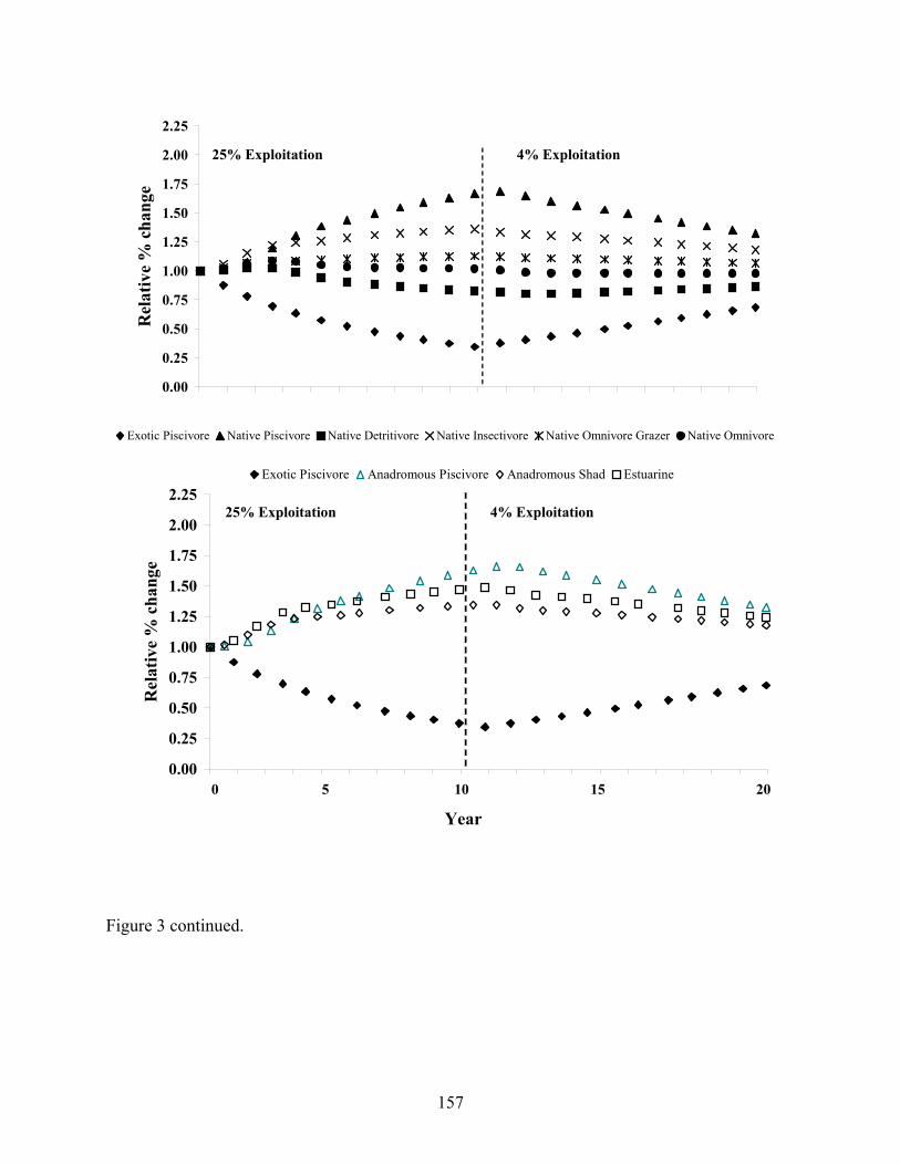
157

0.00

0.25

0.50

0.75

1.00

1.25

1.50

1.75

2.00

2.25R

elat

ive

% c

hang

e

Exotic Piscivore Native Piscivore Native Detritivore Native Insectivore Native Omnivore Grazer Native Omnivore

0.00

0.25

0.50

0.75

1.00

1.25

1.50

1.75

2.00

2.25

Rel

ativ

e %

cha

nge

Exotic Piscivore Anadromous Piscivore Anadromous Shad Estuarine

Figure 3 continued.

0 5 10 15 20

Year

25% Exploitation 4% Exploitation

25% Exploitation 4% Exploitation

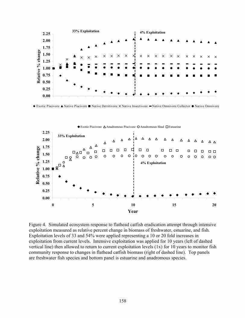
158

0.000.25

0.500.75

1.001.25

1.501.75

2.002.25

1 18 35 52 69 86 103

120

137

154

171

188

205

222

239

Rel

ativ

e %

cha

nge

Exotic Piscivore Native Piscivore Native Detrit ivore Native Insectivore Native Omnivore Collector Native Omnivore

0.00

0.25

0.50

0.75

1.00

1.25

1.50

1.75

2.00

2.25

1 18 35 52 69 86 103

120

137

154

171

188

205

222

239

Rel

ativ

e %

cha

nge

Exotic Piscivore Anadromous Piscivore Anadromous Shad Estuarine

Figure 4. Simulated ecosystem response to flathead catfish eradication attempt through intensive exploitation measured as relative percent change in biomass of freshwater, estuarine, and fish. Exploitation levels of 33 and 54% were applied representing a 10 or 20 fold increases in exploitation from current levels. Intensive exploitation was applied for 10 years (left of dashed vertical line) then allowed to return to current exploitation levels (1x) for 10 years to monitor fish community response to changes in flathead catfish biomass (right of dashed line). Top panels are freshwater fish species and bottom panel is estuarine and anadromous species.

33% Exploitation 4% Exploitation

33% Exploitation

4% Exploitation

0 5 10 15 20

Year

159

0.00

0.25

0.50

0.75

1.00

1.25

1.50

1.75

2.00

2.25

1 18 35 52 69 86 103

120

137

154

171

188

205

222

239

Rel

ativ

e %

cha

nge

Exotic Piscivore Native Piscivore Native Detritivore Native Insectivore Native Omnivore Collector Native Omnivore

54% Exploitation 4% Exploitation

0.00

0.25

0.50

0.75

1.00

1.25

1.50

1.75

2.00

2.25

1 18 35 52 69 86 103

120

137

154

171

188

205

222

239

Rel

ativ

e %

cha

nge

Exotic Piscivore Anadromous Piscivore Anadromous Alosa Estuarine

54% Exploitation 4% Exploitation

Figure 4 continued.

0 5 10 15 20

Year

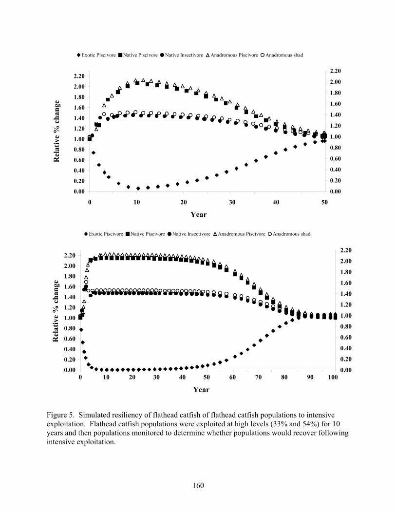
160

0.00

0.20

0.40

0.60

0.80

1.00

1.20

1.40

1.60

1.80

2.00

2.20

1

Rel

ativ

e %

cha

nge

0.00

0.20

0.40

0.60

0.80

1.00

1.20

1.40

1.60

1.80

2.00

2.20

Exotic Piscivore Native Piscivore Native Insectivore Anadromous Piscivore Anadromous shad

0.000.200.400.600.801.001.201.401.601.802.002.20

1 856

Rel

ativ

e %

cha

nge

0.00

0.20

0.40

0.60

0.80

1.00

1.20

1.40

1.60

1.80

2.00

2.20

Exotic Piscivore Native Piscivore Native Insectivore Anadromous Piscivore Anadromous shad

Figure 5. Simulated resiliency of flathead catfish of flathead catfish populations to intensive exploitation. Flathead catfish populations were exploited at high levels (33% and 54%) for 10 years and then populations monitored to determine whether populations would recover following intensive exploitation.

0 10 20 30 40 50

Year

0 10 20 30 40 50 60 70 80 90 100

Year

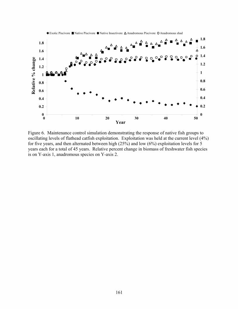
161

0

0.2

0.4

0.6

0.8

1

1.2

1.4

1.6

1.8

1

Rel

ativ

e %

cha

nge

0

0.2

0.4

0.6

0.8

1

1.2

1.4

1.6

1.8Exotic Piscivore Native Piscivore Native Insectivore Anadromous Piscivore Anadromous shad

Figure 6. Maintenance control simulation demonstrating the response of native fish groups to oscillating levels of flathead catfish exploitation. Exploitation was held at the current level (4%) for five years, and then alternated between high (25%) and low (6%) exploitation levels for 5 years each for a total of 45 years. Relative percent change in biomass of freshwater fish species is on Y-axis 1, anadromous species on Y-axis 2.

0 10 20 30 40 50 Year

162

Appendix 1. Estimating population biomass of each functional group.

Population estimates for each functional group were calculated by summing three-

pass removal estimates for each species within that functional group. Often, removal

estimates for an individual species were not possible because catch did not decline with each

sampling pass (as required in a removal estimate, [Seber 1982]). However, at the functional

group level there was usually a decline in group abundance among sampling passes. I

combined the catch of each species, in each pass, within a functional group to create a three-

pass “overall group removal.” I then used this combined removal to estimate capture

probability for that functional group. I then fixed capture probability for each species within

the group to the group-wide capture probability and re-ran the removal model (using a closed

capture model in program MARK) to estimate population size. Population biomass for each

functional group (used in the Ecopath model) was then calculated by assigning an average

weight (based on field measurements) to each species within the functional group, and then

calculating a weighted average biomass for that functional group, weighted by the abundance

of the individual members of the functional group (see text).

Appendix Table 1. Species name, functional group, functional group capture probability, number of individuals of each species caught in each pass, sum of catch from the three passes, estimated population size (fish/km), and standard error for each removal in Contentnea Creek

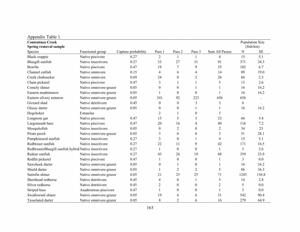
163

Appendix Table 1. Contentnea Creek Spring removal sample

Population Size (fish/km)

Species Functional group Capture probability Pass 1 Pass 2 Pass 3 Sum All Passes N SE Black crappie Native piscivore 0.27 2 1 1 4 15 5.1 Bluegill sunfish Native insectivore 0.27 33 27 31 91 371 24.3 Bowfin Native piscivore 0.47 19 7 9 35 102 6.7 Channel catfish Native omnivore 0.15 4 6 4 14 89 19.0 Creek chubsucker Native omnivore 0.69 24 0 2 26 66 2.3 Chain pickerel Native piscivore 0.47 3 1 1 5 13 2.6 Comely shiner Native omnivore-grazer 0.05 0 0 1 1 16 16.2 Eastern mudminnow Native omnivore-grazer 0.05 1 0 0 1 16 16.2 Eastern silvery minnow Native omnivore-grazer 0.05 341 92 223 656 656 . Gizzard shad Native detritivore 0.45 0 0 3 3 8 . Glassy darter Native omnivore-grazer 0.05 0 0 1 1 16 16.2 Hogchoker Estuarine . 2 1 0 3 . . Longnose gar Native piscivore 0.47 15 5 3 23 66 5.4 Largemouth bass Native piscivore 0.47 20 16 4 40 116 7.2 Mosquitofish Native insectivore 0.05 0 2 0 2 34 23 Pirate perch Native omnivore-grazer 0.05 3 0 0 3 51 28.1 Pumpkinseed sunfish Native insectivore 0.27 3 0 1 4 15 5.1 Redbreast sunfish Native insectivore 0.27 22 11 9 42 171 16.5 RedbreastxBluegill sunfish hybrid Native insectivore 0.27 1 0 0 1 3 2.6 Redear sunfish Native insectivore 0.27 43 26 19 88 359 23.9 Redfin pickerel Native piscivore 0.47 1 0 0 1 3 0.0 Sawcheek darter Native omnivore-grazer 0.05 0 1 0 1 16 16.2 Shield darter Native omnivore-grazer 0.05 1 2 2 5 86 36.3 Satinfin shiner Native omnivore-grazer 0.05 21 25 25 71 1243 136.8 Shorthead redhorse Native detritivore 0.45 4 0 1 5 14 2.8 Silver redhorse Native detritivore 0.45 2 0 0 2 5 0.0 Striped bass Anadromous piscivore 0.47 1 0 0 1 3 0.0 Swallowtail shiner Native omnivore-grazer 0.05 19 6 6 31 542 90.4 Tesselated darter Native omnivore-grazer 0.05 8 2 6 16 279 64.9

164

Appendix Table 1 continued. Contentnea Creek Fall removal sample

Population Size (fish/km)

Species Functional group Capture probability Pass 1 Pass 2 Pass 3 Sum All Passes N SE American shad Anadromous shad . 0 2 3 5 . . Bluegill sunfish Native insectivore 0.25 13 10 9 32 137 15.9 Bowfin Native piscivore . 0 2 2 4 . . Channel catfish Native omnivore . 2 1 2 5 . . Creek chubsucker Native omnivore . 7 0 0 7 . . Coastal shiner Native omnivore-grazer 0.06 0 3 1 4 58 27.0 Eastern silvery minnow Native omnivore-grazer 0.06 5 26 47 78 1150 118.8 Gizzard shad Native detritivore 0.43 0 1 0 1 3 0.0 Hickory shad Anadromous shad . 7 0 0 7 . . Largemouth bass Native piscivore 0.48 18 13 7 38 109 6.8 Longnose gar Native piscivore 0.48 1 3 2 6 15 0.0 Mosquitofish Native insectivore 0.25 1 1 4 6 25 7.0 Mullet Esturarine . 1 1 1 3 . . Pirate perch Native omnivore-grazer 0.06 1 0 0 1 14 13.5 Redbreast sunfish Native insectivore 0.25 15 14 19 48 206 19.5 Redear sunfish Native insectivore 0.25 11 8 13 32 137 15.9 Sawcheek darter Native omnivore-grazer 0.06 1 0 1 2 28 19.0 Shield darter Native omnivore-grazer 0.06 3 0 10 13 191 3.5 Satinfin shiner Native omnivore-grazer 0.06 1 6 2 9 132 40.3 Shorthead redhorse Native detritivore 0.43 3 2 2 7 20 3.5 Silver redhorse Native detritivore 0.43 1 1 0 2 5 0.0 Tesselated darter Native omnivore-grazer 0.06 2 9 20 31 456 74.9 Warmouth Native insectivore 0.25 0 1 0 1 3 0.0

165

Appendix Table 2. Model parameter estimates used in the mass-balance Ecopath model. Functional group name Biomass in habitat area (t/km²) Source

Exotic piscivore 0.237 This study Native piscivore 0.165 This study Native detritivore 0.022 This study Native insectivore 0.185 This study Native omnivore collector 0.390 This study Native omnivore 0.025 This study Anadromous piscivore 0.003 This study Anadromous shad 0.035 This study Estuarine 0.015 This study Invertebrates 4.000 Range from Waters 1977 Plankton 1.000 Range from literature Detritus 100.00 Range from literature

Functional group name Production/ biomass Source Exotic piscivore 0.150 This study, catch-curve Native piscivore 1.050 This study, multiple 3-pass removals Native detritivore 1.750 This study, multiple 3-pass removals Native insectivore 2.800 This study, multiple 3-pass removals Native omnivore collector 1.890 This study, multiple 3-pass removals Native omnivore 1.750 This study, multiple 3-pass removals Anadromous piscivore 2.000 This study, multiple 3-pass removals Anadromous shad 2.200 This study, multiple 3-pass removals Estuarine 2.600 This study, multiple 3-pass removals Invertebrates 5.500 Range from Waters 1977 Plankton 35.000 Range from literature Detritus -

Functional group name Consumption/ biomass (per year) Source Exotic piscivore 3.600 Fishbase Native piscivore 3.930 Fishbase Native detritivore 14.100 Fishbase Native insectivore 10.000 Fishbase Native omnivore collector 36.700 Fishbase Native omnivore 4.800 Fishbase Anadromous piscivore 6.000 Fishbase Anadromous shad 5.000 Fishbase Estuarine 10.000 Fishbase Invertebrates 16.500 Fishbase Plankton - Not estimable Detritus - Not estimable

166

Appendix Table 2 continued. Diet percent-composition for each functional group. Exotic piscivore functional group information is based on diet samples collected in this study, while other groups are estimated from the literature. Exotic

piscivore Native piscivore

Native detritivore

Native insectivore

Native omnivore- collector

Native omnivore

Anadromous piscivore

Anadromous shad

Estuarine Invertebrates Plankton Detritus

Exotic piscivore

0.0% 0.4% 0.4% 35.0% 31.0% 1.2% 0.0% 5.0% 2.5% 24.5% 0.0% 0.0%

Native piscivore

0.0% 10.0% 5.0% 27.5% 20.0% 5.0% 0.0% 5.0% 2.5% 25.0% 0.0% 0.0%

Native detritivore

0.0% 0.0% 0.0% 0.0% 0.0% 0.0% 0.0% 0.0% 0.0% 0.0% 0.0% 100.0%

Native insectivore

0.0% 0.0% 0.0% 0.0% 0.0% 0.0% 0.0% 0.0% 0.0% 50.0% 40.0% 10.0%

Native omnivore- collector

0.0% 0.0% 0.0% 0.0% 0.0% 0.0% 0.0% 0.0% 0.0% 40.0% 40.0% 20.0%

Native omnivore

0.0% 0.0% 0.0% 5.0% 5.0% 0.0% 0.0% 0.0% 0.0% 50.0% 0.0% 40.0%

Anadromous piscivore

0.0% 0.0% 10.0% 25.0% 35.0% 5.0% 0.0% 0.0% 5.0% 20.0% 0.0% 0.0%

Anadromous shad

0.0% 0.0% 0.0% 0.0% 0.0% 0.0% 0.0% 0.0% 0.0% 0.0% 80.0% 20.0%

Estuarine 0.0% 0.0% 0.0% 0.0% 20.0% 0.0% 0.0% 0.0% 0.0% 40.0% 10.0% 30.0%

Invertebrates 0.0% 0.0% 0.0% 0.0% 0.0% 0.0% 0.0% 0.0% 0.0% 0.0% 0.0% 100.0%

167

Appendix Table 2 continued. Functional group name Diet information source Exotic piscivore This study

Native piscivore Davies 1981; Fishbase

Native detritivores Fishbase

Native insectivore Fishbase

Native omnivore-collector Fishbase

Native omnivore Fishbase

Anadromous piscivore Neal et al. 1999; Fishbase

Anadromous shad Fishbase

Estuarine Fishbase

Invertebrates Assumed

Plankton Assumed

Detritus Not estimable

168

CHAPTER 6

SYNTHESIS AND DIRECTION OF FUTURE RESEARCH

169

Synthesis

Based on the results presented in this dissertation, I conclude that introduced flathead

catfish populations in North Carolina have likely altered native fish community biomass

through both predatory and competitive interactions. I developed this conclusion based on

estimates of flathead catfish population size (Chapters 2, 3), diet information (Chapter 4), and

simulation models based on empirical diet information, native fish community composition

and abundance, and flathead catfish exploitation levels from native populations (Chapter 5).

I found that flathead catfish population size in coastal North Carolina rivers can be assessed

using a robust design population model as outlined in Chapters 2 and 3. The robust design

model performed well because I was able to account for temporary emigration by flathead

catfish, which would not be possible with closed or open population models. Population size

estimates for flathead catfish in my study (4-31 fish/km) were within the broad range of sizes

previously reported for both native and introduced riverine populations (Chapter 3).

Estimated population size of introduced flathead catfish populations in the coastal North

Carolina rivers I examined are smaller than in other introduced populations in the

southeastern US (Chapter 3).

I found that in coastal North Carolina rivers, flathead catfish are strict, obligate

carnivores that mainly feed on other fishes and crayfish. When available, flathead catfish

also utilize marine derived fish and invertebrate food resources. The use of these resources

by flathead catfish could be particularly important in planning restoration efforts for

anadromous species in coastal rivers with flathead catfish populations.

I combined demographic information for flathead catfish and the native fish

community, with diet information for both groups, in an ecosystem simulation model to

170

examine the interactions between flathead catfish and the native fish community. These

simulation models indicate that flathead catfish have altered native fish communities via both

direct predation of, and indirect competition with, native fishes. However, these impacts

might be mitigated through intensive harvest of flathead catfish at levels similar to those

found for native flathead catfish populations, about 10-25%.

Aquatic Invasion Rules

Moyle and Light (1996) developed a series of empirical “rules” to predict the fate of

species introduced in stream and estuarine environments. Although originally derived for

California waters, several of these rules appear to characterize the flathead catfish invasion

along the Atlantic slope. I review these rules below as a framework in which to summarize

my findings and describe areas of future research that could be used to develop testable

hypotheses to further our understanding of invasive species in aquatic environments.

Moyle and Light (1996) Rule: Most invaders fail to become established.

While most invasions fail, those that have been successful are often predators

(particularly piscivores) (Moyle and Light 1996). Flathead catfish are well established in the

coastal rivers I examined as evident by the range of sizes collected and population size

estimates. Given the low detectability for flathead catfish in coastal rivers (Chapter 3), they

may be established elsewhere, but not yet detected.

Moyle and Light (1996) Rule: In the long term, or in relatively undisturbed aquatic systems, success of an invader will depend on a close match between its physiological and life history requirements and the characteristics of the system being invaded.

Many invasive fish species are part of a small group of widely and frequently

introduced sportfish, including flathead catfish (Moyle 1986; Heidinger 1993; Moyle and

Light 1996). These sportfish species have successfully invaded new systems and established

171

self-sustaining populations not because of some intrinsic adaptability of these species, but

instead, their success is a function of the frequency which they have been introduced and the

successful pairing of the introduced species with the environment in which it is released–

often by well meaning anglers or management agencies (Moyle 1986; Moyle and Light

1996).

Moyle and Light (1996) Rule: Most successful invaders are integrated without major negative effects (e.g., extirpations) on the communities being invaded.

While I have no evidence of any native fish species extirpations related to direct

predation by flathead catfish within the rivers I studied, I was able to demonstrate (via

simulation modeling, Chapter 5) that flathead catfish have probably caused reductions in

native fish biomass via both competitive and predatory interactions (Chapters 4, 5). Invasive

piscivorous fish have been shown to alter native fish assemblages in other systems (White

and Harvey 2001), and although my results are derived from simulations, they provide

guidance into how the native fish community would respond to reductions in flathead catfish

biomass through intensive exploitation– a widely considered management action for

introduced flathead catfish populations.

Moyle and Light (1996) Rule: Major community effects of invasions are most often observed where the number of species is low.

The impact on native fish communities following flathead catfish introduction may

primarily be a function of the type of system into which they are introduced. Thus, the

greatest impact of flathead catfish predation likely occurs in relatively unproductive systems

(e.g., small streams and rivers, many with few species) while their impact may not be as

noticeable in larger systems with more species. This rule was originally developed for high

mountain California streams with only 5-7 fish species, but it may apply here in systems with

172

more (20-30) species. The availability of anadromous and estuarine food items for flathead

catfish in Contentnea Creek and the Northeast Cape Fear River may lessen the impact of

flathead catfish predation on native fishes as compared to that in the Lumber River. These

marine based prey items may serve as flathead catfish predation buffers to the native fish

community. Thus, flathead catfish in the Lumber River, with fewer available prey species,

may concentrate their feeding pressure on a smaller group of species, potentially causing

greater change to the native fish community and making their impact more readily apparent

(Chapters 4, 5).

Moyle and Light (1996) Rule: In aquatic systems with intermediate levels of human disturbance, any species with the right physiological and morphological characteristics can become established.

Flathead catfish are not the only aquatic invasive species in each of these river

systems. Several of the identifiable prey items in my study and that of Guier et al. (1981)

were themselves introduced species into the mid-Atlantic slope. These species included

redear sunfish, blue catfish, and flathead catfish. The Neuse River drainage supports 20

aquatic invasive species, the Cape Fear River drainage contains 31, while the Little Pee Dee

“only” supports 11. Disturbed aquatic ecosystems are more likely than undisturbed systems

to support invasive species (Moyle and Light 1996). Both the Neuse and the Northeast Cape

Fear rivers are anthropogenically impacted rivers (nutrient enrichment, sedimentation, flow

regime alterations; Cahoon et al. 1999; Paerl et al. 2001), while large portions of the Lumber

River retain “National Wild and Scenic River” status from the US National Park Service for

their relatively pristine condition.

173

Future Research

My simulation results suggesting positive responses in native fish biomass following

flathead catfish harvest could be considered as a part of a broader ecosystem restoration

effort to mitigate the variety of anthropogenic ecosystem alterations in coastal rivers. While

many aspects of coastal river ecosystem restoration remain in an experimental phase

(Lenihan et al. 1999), our ability to harvest fish populations is well established, and directed

harvest toward flathead catfish may represent a conceptually simple, but important step in

helping restore degraded ecosystems. Interest in flathead catfish as a sportfish within both

native and introduced river systems is growing as evident by the increasing number of

popular press publications devoted to this species, increasing specialization among angler

groups (including tournaments), and the creation of specialized fishing equipment designed

to target large catfish (Quinn 1993; Jackson 1999). Efforts should be made to encourage

these developing fisheries and to monitor angler effort, expectations, and ecosystem response

to flathead catfish harvest. Future research along the Atlantic slope should also focus on

understanding the linkages flathead catfish create between marine and freshwater foodwebs.

Efforts should also be made to determine if in the absence of marine derived food resources,

flathead catfish have a greater impact on native fish communities.

Flathead catfish are a remarkable animal, capable of eliciting excitement, and even

respect, from both resource users and managers in native and introduced ecosystems. These

attitudes towards an animal with few charismatic qualities (to some) may stem largely

because of their ability to attain large physical size, potential to restructure ecosystems, and

maybe even from the mystery that surrounds large aquatic animals that we cannot readily see

and do not completely understand. Although my research has provided new information on

174

this species in coastal North Carolina rivers, much remains to be learned about this amazing

creature by future researchers fortunate to work with this species.

175

References

Cahoon, L. B., J. A. Mikucki, and M. A. Mallin. 1999. Nitrogen and phosphorus imports to the Cape Fear and Neuse river basins to support intensive livestock production. Environmental Science and Technology 33:410-415.

Heidinger, R. C. 1993. Stocking for sport fisheries enhancement. Pages 309-334 in C. C.

Kohler, and W. A. Hubert, editors. Inland fisheries management in North America. American Fisheries Society, Bethesda, Maryland.

Jackson, D. C. 1999. Flathead catfish: biology and management. Pages 23-36 in E. R.

Irwin, W. A. Hubert, C. F. Rabini, H. L. Schramm, Jr., and T. Coon, editors. Catfish 2000: proceedings of the international ictalurid symposium. American Fisheries Society, Symposium 24, Bethesda, Maryland.

Lenihan, H. S., F. Micheli, S. W. Shelton, C. H. Peterson. 1999. The influence of

multiple environmental stressors on susceptibility to parasites: An experimental determination with oysters. Limnology and Oceanography 44:910-924.

Moyle, P. B. 1986. Fish introductions into North America: Patterns and ecological impact.

Pages 27-43 in H. A. Mooney and J. A. Drake, editors. Ecology of biological invasions of North America and Hawaii. Springer, New York.

Moyle, P. B., and T. Light. 1996 A. Biological invasions of fresh water: empirical rules

and assembly theory. Biological Conservation 78:149-161. Quinn, S. P. 1993. Description of a multiple use fishery for flathead catfish. North

American Journal of Fisheries Management 13:594-599. Paerl, H. W., J. D. Bales, L. W. Ausley, C. P. Buzzelli, L. B. Crowder, L. A. Eby, J.

M. Fear, M. Go, B. L. Peierls, T. L. Richardson, J. S. Ramus. 2001. Ecosystem impacts of three sequential hurricanes (Dennis, Floyd, and Irene) on the United States’ largest lagoonal estuary, Pamlico Sound, NC. Proceedings of the National Academy of Science 98:5655-5660.

White, J. L., and B. C. Harvey. 2001. Effects of an introduced piscivorous fish on native

benthic fishes in a coastal river. Freshwater Biology 46:987-995.