parametric transition of stationary and axisymmetric ... · parametric transition of stationary and...
TRANSCRIPT
Parametric Transition of Stationaryand Axisymmetric Bodies to Black
Holes
Dissertationzur Erlangung des akademischen Gradesdoctor rerum naturalium (Dr. rer. nat.)
vorgelegt dem Rat der Physikalisch-AstronomischenFakultat der Friedrich-Schiller-Universitat Jena
von M.Sc. Hendrick Labranchegeboren am 2. Juli 1979 in Quebec, Kanada
Gutachter
1. Prof. Dr. Reinhard Meinel (Friedrich-Schiller-Universitat Jena)
2. PD Dr. Claus Lammerzahl (Universitat Bremen)
3. Prof. Dr. Jutta Kunz (Carl von Ossietzky Universitat Oldenburg)
Tag der Disputation: 11. Mai 2010

Contents
Zusammenfassung (auf Deutsch) iii
Abstract (in English) iv
1. Introduction 1
2. An Overview of Stationary and Axisymmetric Spacetimes 4
2.1. The Metric Potentials and the Einstein Equations . . . . . . . . . . . . . 4
2.1.1. The Metric of Stationary and Axisymmetric Spacetimes . . . . . . 4
2.1.2. Uniformly Rotating Cold Perfect Fluids as Gravitational Source . 5
2.1.3. The Einstein Field Equations . . . . . . . . . . . . . . . . . . . . 7
2.2. The Vaccum Domain . . . . . . . . . . . . . . . . . . . . . . . . . . . . . 8
2.2.1. The Ernst Equation . . . . . . . . . . . . . . . . . . . . . . . . . 9
2.2.2. The Multipole Moments . . . . . . . . . . . . . . . . . . . . . . . 10
2.3. The Black Hole Limit of Fluid Bodies in Equilibrium . . . . . . . . . . . 11
2.3.1. Necessary and Sufficient Condiditions for a Black Hole Limit . . . 12
2.3.2. The Extreme Kerr Black Hole Geometry . . . . . . . . . . . . . . 14
3. Strange Matter Stars and their Parametric Transition to a Black Hole 17
3.1. Model and Method used for Relativistic Strange Stars . . . . . . . . . . . 17
3.1.1. Equation of State . . . . . . . . . . . . . . . . . . . . . . . . . . . 17
3.1.2. The Ansorg-Kleinwachter-Meinel Numerical Method . . . . . . . . 20
3.2. Solutions of Strange Quark Matter . . . . . . . . . . . . . . . . . . . . . 21
3.2.1. The Schwarzchild Class of Strange Quark Matter . . . . . . . . . 21
3.2.2. The Ring Class of Strange Quark Matter . . . . . . . . . . . . . . 27
3.3. Parametric Transition to a Black Hole . . . . . . . . . . . . . . . . . . . 28
3.3.1. Multipole Moments of Rings . . . . . . . . . . . . . . . . . . . . . 28
3.3.2. Throat Geometry . . . . . . . . . . . . . . . . . . . . . . . . . . . 35
3.3.3. Escape Energy . . . . . . . . . . . . . . . . . . . . . . . . . . . . 36
i
Contents ii
4. Ernst Potentials near the Black Hole Limit 41
4.1. Reformulation of the Conjecture . . . . . . . . . . . . . . . . . . . . . . . 41
4.1.1. Normalized Multipoles . . . . . . . . . . . . . . . . . . . . . . . . 41
4.1.2. The Multipoles and the First Law of Thermodynamics . . . . . . 43
4.1.3. A Taylor Series Near the Black Hole Limit . . . . . . . . . . . . . 45
4.2. Ernst Potential of the Kerr Black Hole . . . . . . . . . . . . . . . . . . . 47
4.3. Ernst Potential of the Uniformly Rotating Disk of Dust . . . . . . . . . . 49
4.3.1. Ernst Potential of the Disk . . . . . . . . . . . . . . . . . . . . . . 50
4.3.2. Ernst Potential of the Disk in the Black Hole Limit . . . . . . . . 53
4.3.3. Derivatives of the Ernst Potential in the Black Hole Limit . . . . 54
4.4. Taylor Series of the Disk . . . . . . . . . . . . . . . . . . . . . . . . . . . 60
4.4.1. Series of Functions of µ . . . . . . . . . . . . . . . . . . . . . . . . 61
4.4.2. Series of Functions of (µ, ζ) . . . . . . . . . . . . . . . . . . . . . 62
4.4.3. Series of the Ernst Potential of the Disk . . . . . . . . . . . . . . 69
5. Conclusion 75
Bibliography 77
A. Elliptic Integrals and Functions 81
B. Some Useful Functions for the Disk of Dust 84
B.1. List of Functions in the Ernst Potential of the Disk . . . . . . . . . . . . 84
B.2. Some Other Useful Relations . . . . . . . . . . . . . . . . . . . . . . . . . 86
Danksagung 87
Ehrenwortliche Erklarung 88
Lebenslauf 89
Zusammenfassung
Diese Dissertation behandelt Losungen stationarer und axialsymmetrischer Korper und
ihren parametrischen Ubergang zu Schwarzen Lochern. Numerische Losungen von Flus-
sigkeiten im Gleichgewicht werden unter Annahme einer “strange quark matter”-Zu-
standsgleichung mit sehr hoher Genauigkeit berechnet. Verschiedene Sequenzen von
Konfigurationen werden fur spharoidale und toroidale Korper untersucht, um die wesent-
lichen Eigenschaften dieser Familie von Objekten aus “strange matter” aufzuzeigen.
Konfigurationen mit maximaler Masse und maximalem Drehimpuls wurden in der Nahe
von - aber nicht an - der “mass-shedding”-Grenze gefunden, im Gegensatz zu den Er-
wartungen.
Außerdem zeigen wir, dass “strange matter”-Ringe einen kontinuierlichen Ubergang
zur extremen Kerr-Losung erlauben. Die von Geroch und Hansen definierten Multi-
polmomente wurden untersucht und deuten auf ein universelles Verhalten von Korpern
hin, die sich parametrisch der extremen Kerr-Losung annahern. Das Auftreten einer
“throat geometry” als charakteristisches Merkmal der extremen Kerr-Raumzeit wird
diskutiert. Dann zeigen wir, im Hinblick auf die Stabilitat, dass ein Testteilchen, das
auf der Oberflache des Ringes liegt, niemals genug Energie besitzt, um entlang einer
Geodaten ins Unendliche zu gelangen.
Ausgehend vom universellen Verhalten, welches die Multipolmomente andeuten, for-
mulieren wir eine Vermutung bezuglich der parametrischen Annaherung gleichformig
rotierender Flussigkeiten an die extreme Kerr-Losung. Die Vermutung wird fur ein Mul-
tipolmoment (den Drehimpuls) anhand eines “thermodynamischen Gesetzes” beschrie-
ben, welches fur alle gleichformig rotierenden Flussigkeiten im Gleichgewicht gilt. Die
selbe Vermutung wird dann in ihrer Gesamtheit fur die Staubscheibe gezeigt.
Abschließend wird das Ernst-Potential der Staubscheibe auf der Achse in eine Taylor-
Reihe in der Umgebung der extremen Kerr-Losung entwickelt. Diese Reihe scheint
uberall auf der Achse zu konvergieren, ausgehend vom Grenzfall des Schwarzen Lochs
bis hin zur Newton’schen Grenze der Scheibenlosung, außerhalb einer kleinen Region in
der Nahe der Scheibe. Die benutzte Methode erlaubt es uns sehr effizient, die Reihe in
beliebig hoher Ordnung zu entwickeln.
iii
Abstract
This thesis deals with solutions of stationary and axisymmetric relativistic bodies and
their parametric transition to black holes. Highly accurate numerical solutions were pro-
duced for perfect fluids in equilibrium made of strange quark matter. Several sequences
of configurations, including spheroidal bodies and rings, were produced to sketch the
main features of the family of strange matter bodies. The maximal mass and maximal
angular momentum configurations were found close to but not at the mass-shedding
limit, contrary to what was believed.
We also show numerically that strange matter rings permit a continuous transition
to the extreme Kerr black hole. The multipoles as defined by Geroch and Hansen
are studied and suggest a universal behaviour for bodies approaching the extreme Kerr
solution parametrically. We discuss the appearence of a “throat geometry”, a distinctive
feature of the extreme Kerr spacetime. Then we verify, with regard to stability, that a
particle sitting on the surface of the ring never has enough energy to escape to infinity
along a geodesic.
From the universal behaviour suggested by the multipoles, we formulate a conjecture
related to the parametrical approach of uniformly rotating fluids to the extreme Kerr
black hole. The conjecture is explained for one multipole (the angular momentum) using
a “law of thermodynamics” valid for all uniformly rotating bodies in equilibrium. The
same conjecture is then proved in its entirety for the disk of dust.
Finally, the Ernst potential on the axis of the disk of dust is expanded in a Taylor
series anchored at the extreme Kerr black hole limit. This series seems to converge
everywhere on the axis, from the black hole limit to the Newtonian limit of the disk
solution, except for a tiny region near the disk. The method used allows us to generate
the series efficiently to arbitrarily high orders.
iv
1. Introduction
Once stars exhaust their capacity to generate energy through thermonuclear reactions,
it is understood that they die by a variety of dynamical prosesses, which combine rapid
ejection of matter and contraction of the stellar core. Depending mainly on the initial
mass of the star, its final remnant is expected to be either a white dwarf, a neutron
star or a black hole. These remnants and the dynamical processes leading to them are
all configurations where relativistic effects are important, so relevant modelling needs to
be done in full accordance with general relativity. The dynamical transition to a stellar
remnant is still today an arduous task and not completely understood, but interesting
achievements have been published. Making use of the introduction of a local (3-D)
and dynamic notion of a “horizon” such as is described in [AK04], numerical work has
followed the collapse of an initial distribution of matter to a “black hole”, see e.g. [Fon03].
For sufficiently long run-times, a (4-D) event horizon can be located a postiori and there
exist simulations, e.g. [BHM+05], supporting the widely held expectation that after
collapse, the configuration will settle down to a Kerr black hole. Many questions are
still open however regarding the initial data, the matter model, the accuracy of the time
evolution, etc.
On the other hand, the modelling of the final remnants is a much easier task and
better understood, since the computation can take advantage of symmetries such as
stationarity, axial and equatorial symmetries, and because of the extremely high Fermi
energy expected for the degenerate fermion gas in white dwarfs and neutron stars, we
can assume that their particles have zero temperature. Many discussions conclude that
relativistic stellar models made of uniformly rotating cold perfect fluids are indeed rea-
sonable simplifications of real astronomical stars such as neutron stars [Lin92,MAK+08].
Within the class of stationary and axisymmetric bodies, the static cases (non-rotating
bodies) are the easiest to model and the best known properties are often found from
(and sometimes restricted to) this category. Among these interesting properties, it was
found that between static white dwarfs, neutron stars and black holes, no “smooth”
(quasi-static) transition exists: such transitions imply dynamical collapses. One of these
transitions assumes that the electron-degeneracy pressure in white dwarfs must fail near
the so-called “Chandrasekhar limit” [Cha31] and the dwarf must suddently collapse into
1
1. Introduction 2
a neutron star. For the second transition, the equation of state (EOS) of neutron stars
is still very speculative today, but under the assumption that the energy density in the
star does not increase outwards, it can be shown that stars in hydrostatic equilibrium
must satisfy the so-called “Buchdahl inequality”: they must have a radius greater than
9/8 times the radius1 of a black hole with the same mass [Buc59]. So a static star can
become a black hole only through the process of a dynamical collapse. Contrary to the
dynamics of the first transition, which is dependent on our knowledge of the EOS, the
dynamical collapse in the second transition is valid for any relevant EOS.
This “Buchdahl inequality” is true only for static stars, but it would be legitimate to
ask if, for the entire class of stationary and axisymmetric bodies, a smooth or “quasi-
stationary” transition between a star and a black hole could exist. In [Mei04,Mei06],
necessary and sufficient conditions for a quasi-stationary transition were presented and
it was proved that an extreme Kerr black hole necessarily results. Using the analytic
solution for the relativistic disk of dust [NM95], a transition to a black hole was found
explicitly [Mei02]. Transitions have also been found numerically for rings with a variety
of EOS [AKM03b,FHA05].
In this thesis, we want to investigate in detail the parametric (or quasi-stationary)
transition of stationary and axisymmetric bodies to black holes. Such a transition is
not plagued by all the problems of modelling dynamical collapses, but at the price of
being very highly idealized. A parametric sequence of configurations can at best model
a “non-dynamic” collapse. In astrophysical collapse scenarios, there may well be matter
that does not fall into the centre, and the time evolution of a non-stationary spacetime
will determine how gravitational radiation leaves the system and leads to changes in the
angular momentum of the central region. Thus the transition to a black hole considered
in this work should be seen as an instructive limit capable of shedding some light on
issues regarding the path matter could take in evolving to a black hole.
The conditions for a quasi-stationary transition between a star and a black hole de-
pends on the gravitational potential at the surface of the star, but not directly on the
EOS. So many stellar models with different EOS can be candidates for a parametric
transition to black holes. For this work, we wanted to focus our investigation on a stel-
lar model with an astrophysically plausible EOS. Among the several running candidates
for EOS of neutron stars, we decided to focus on a stellar model made of strange quark
matter: a type of “neutron star” made of equal numbers of deconfined up, down and
strange quarks.
1radius in Schwarzschild coordinates
1. Introduction 3
The work that we present here is planned as follows. We begin by summarizing in
Chapter 2 the essential concepts and equations of general relativity that are needed for
our work. Then, our investigation is divided in two parts.
In a first part (Chapter 3), we present solutions of a star model made of strange quark
matter. The first pages are devoted to a brief description of the equation of state used
here to model strange matter and the numerical method that we use to compute solutions
(Sec. 3.1). Then, sequences of solutions are presented, for strange stars with spheroidal
and toroidal topologies, and some extremal configurations are discussed (section 3.2).
Finally, we follow the progression of multipole moments of rings as they tend to those of
the extreme Kerr black hole, we discuss the appearance of a “throat region” separating
an “inner” from an “outer world”, and we verify numerically that a particle resting on
the ring’s surface is always gravitationally bound, a condition, which can be considered
to be a minimal requirement for stability (Sec. 3.3).
In a second part (Chapter 4), we explore a property of the Ernst potential that fluid
bodies in equilibrium share with black holes near the extreme Kerr black hole limit. This
property, which is conjectured in chapter 3, is partially explained by a “thermodynamical
law” and can take a nice form if the Ernst potential is written as a Taylor series with a
suitable choice of normalized coordinates (Sec. 4.1). As an example, we write down the
beginning of this Taylor series for the Ernst potential of the Kerr black hole (Sec. 4.2). We
prove that this conjecture indeed holds for the uniformly rotating disk of dust (Sec. 4.3).
And finally, we generate a Taylor series for the Ernst potential of the disk of dust near
its black hole limit (Sec. 4.4).
Throughout this thesis, units are used in which the gravitational constant G and
speed of light c are equal to one, and our sign convention of the metric signature is
(+, +, +,−).
2. An Overview of Stationary and Axisymmetric
Spacetimes
This chapter gives a quick and concise overview of the concepts and equations of general
relativity for stationary and axisymmetric spacetimes. It shows the essential information,
definitions and conventions that we make use for this work. For further information on
the theory of equilibrium configurations of rotating fluids, we recommend you to refer
to the book Relativistic Figures of Equilibrium [MAK+08].
2.1. The Metric Potentials and the Einstein Equations
2.1.1. The Metric of Stationary and Axisymmetric Spacetimes
A spacetime with axial symmetry and stationarity requires that the metric potentials gµν
be independent of a time coordinate t and an azimuthal angle ϕ. Restricting ourselves
to spacetimes filled only by vacuum and a rigidly rotating perfect fluid, a decomposition
of the metric into orthogonal 2-spaces becomes possible by virtue of the theorem given
in [KT66].1 The line element for such spacetimes can be written, with use of the Lewis-
Papapetrou coordinates, in the form
ds2 = e−2U [e2k(dρ2 + dζ2) + W 2dϕ2] − e2U(adϕ + dt)2, (2.1)
with the functions e2k, e2U , W and a depending on ρ and ζ only. The equatorial plane is
given by ζ = 0 and the axis of rotation by ρ = 0. These potentials should behave in such
a way that the metric becomes the Minkowski metric at spatial infinity (ρ2 + ζ2 → ∞)
and also corresponds to Newton’s theory of gravity far from the gravitational source:
gtt = −e2U = −1 +2M
r+ O
( 1
r2
), (2.2a)
gtϕ = −ae2U = −2J sin2 θ
r+ O
( 1
r2
), (2.2b)
1This is the so-called “circularity condition”, which holds for a large class of energy-momentum tensor.which includes rigidly rotating perfect fluid bodies.
4
2. An Overview of Stationary and Axisymmetric Spacetimes 5
gϕϕ = W 2e−2U − a2e2U = r2 sin2 θ[1 + O
( 1
r2
)], (2.2c)
gρρ = gζζ = e2k−2U = 1 +2M
r+ O
( 1
r2
)(2.2d)
where M and J are respectively the gravitational mass and the angular momentum, and
where we use r :=√
ρ2 + ζ2 and tan θ := ρ/ζ . Since we want to deal with uniformly
rotating sources, we introduce a coordinate system with a constant angular velocity Ω
around the rotation axis with respect to the frame of an observer at infinity:
ρ′ = ρ , ζ ′ = ζ , ϕ′ = ϕ − Ωt , t′ = t . (2.3)
The metric potentials of the “rotating frame” are related to those of the “non-rotating
frame” as follow:
e2U ′
= e2U [(1 + Ωa)2 − Ω2W 2e−4U ] , (2.4a)
(1 − Ωa′)e2U ′
= (1 + Ωa)e2U , (2.4b)
e2k′−2U ′
= e2k−2U (2.4c)
and W ′ = W is unaffected by the coordinate transformation.
2.1.2. Uniformly Rotating Cold Perfect Fluids as Gravitational Source
If we consider a perfect fluid body in thermodynamic equilibrium as the source of the
gravitational field, the energy-momentum tensor becomes
T αβ = (ǫ + p)uαuβ + p gαβ, (2.5)
where uα, ǫ and p are respectively the 4-velocity field, the energy density and the pressure
of the fluid.2
The independence of the metric potentials in (2.1) on the time t and the azimuthal
angle ϕ can be expressed using two associated Killing vectors: ξα = (0, 0, 0, 1) for
stationarity and ηα = (0, 0, 1, 0) for axisymmetry; the order of the components follows
xα = (ρ, ζ, ϕ, t). For solutions that are strictly stationary and axially symmetric, the
source must be in thermodynamic equilibrium, which is achieved for a fluid of zero
temperature and rigid rotation, and the 4-velocity must follow a time-like direction
which is a linear combination of the two Killing vectors. To satisfy all these conditions,
2Greek indices run from 1 to 4.
2. An Overview of Stationary and Axisymmetric Spacetimes 6
the 4-velocity field must be
uα = e−U ′
(ξα + Ω ηα) = e−U ′
(0, 0, Ω, 1) or u′α = e−U ′
(0, 0, 0, 1) (2.6)
where uα and u′α are respectively in the frame of an observer at infinity and in the
“co-rotating frame” (rotating with the fluid), and we see that Ω becomes the angular
velocity of the source with respect to infinity. For a fluid in hydrostatic equilibrium, the
constant Ω can be expressed through several different concepts [HS67]:
Ω =dϕ
dt=
uϕ
ut= − ∂ ut
∂ uϕ=
∂M
∂J
∣∣∣∣MB=constant
,
where the two last partial derivatives refer to nearby configurations in equilibrium, with
MB being the baryonic mass of the source.
The baryonic mass, the angular momentum J and the gravitational mass M can
be obtained from the energy-momentum tensor with the following integrals over a 3-
dimensional volume containing the source:
MB = 2π
∫∫ǫB e2k′−3U ′
W dρ dζ , (2.7a)
J = − 2π
∫∫(ǫ + p) a′ e2(k′−U ′) W dρ dζ , (2.7b)
M = 2ΩJ + 2π
∫∫(ǫ + 3p) e2(k′−U ′) W dρ dζ , (2.7c)
where ǫB is the baryonic mass density, corresponding to the total energy density of a
volume element less the internal energy density (ǫB = ǫ − ǫint). The mass and angular
momentum from the volume integrals are the same as those measured in the asymptotic
behaviour at infinity in Eqs(2.2) [HS67], so the two methods of measurement provide an
important test of consistency for numerical solutions.
To describe the surface of a fluid body, the co-rotating potential U ′ has a useful
and intuitive meaning: the function is constant along isobaric surfaces. We rename the
potential V ≡ U ′, and the surface of the fluid body, defined to be the surface of vanishing
pressure, can thus be denoted by V = V0. The constant V0 is related to the relative
redshift Z0, the redshift of zero angular momentum photons emitted from the surface of
the body and observed at infinity:
e−V0 − 1 = Z0. (2.8)
2. An Overview of Stationary and Axisymmetric Spacetimes 7
For zero temperature fluid bodies, one can relate the baryonic mass density ǫB to ǫ and
p through
ǫB =ǫ + p
h(p), (2.9)
where h(p) is the specific enthalpy, and has the property that at any location in the
source, the product h(p) eV is always constant.
Nearby configurations in equilibrium with the same equation of state are related by
a law which looks like an analogue of the first law of thermodynamics at zero tempera-
ture [HS67]:
dM = ΩdJ + µcdMB , µc = h(0) eV0 . (2.10)
For sequences of constant angular momentum J , which contain an extremum of the
gravitational mass M within the sequence, it can be shown from the last equation that
the configuration with extremal M marks a limit of stability, provided that there exists
a dissipative mechanism which conserves J and MB. The unstable part of the sequence
near the extremum can be identified by the condition
d2M
dM2B
> 0 . (2.11)
With the arbitrary 4-velocity uα of a test particle and the Killing vector ξα correspond-
ing to stationarity, one can define the specific energy of a test particle with respect to
infinity, i.e. the energy per unit mass, as E = −uαξα, which is a conserved quantity
along any geodesic. For a fluid element, the specific energy is thus
E = −uαξα = eV (1 − Ωa′) . (2.12)
This quantity can tell us how the matter is gravitationally bound. If E < 1, then the
test particle is bound and cannot escape to infinity on a geodesic; if E > 1, then the
particle has enough energy to escape.
2.1.3. The Einstein Field Equations
The computation of the Einstein field equations (without cosmological constant)
Rαβ − 1
2Rgαβ = 8πT αβ
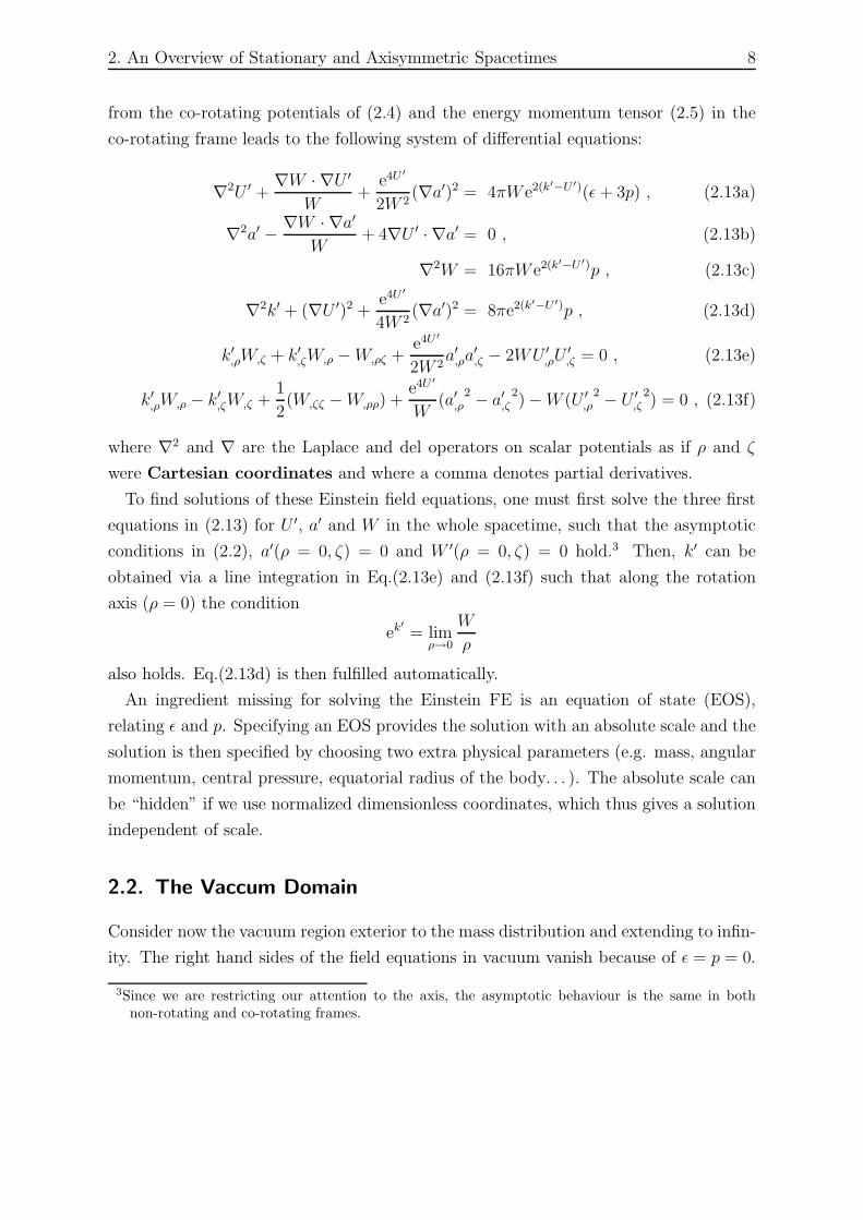
2. An Overview of Stationary and Axisymmetric Spacetimes 8
from the co-rotating potentials of (2.4) and the energy momentum tensor (2.5) in the
co-rotating frame leads to the following system of differential equations:
∇2U ′ +∇W · ∇U ′
W+
e4U ′
2W 2(∇a′)2 = 4πW e2(k′−U ′)(ǫ + 3p) , (2.13a)
∇2a′ − ∇W · ∇a′
W+ 4∇U ′ · ∇a′ = 0 , (2.13b)
∇2W = 16πW e2(k′−U ′)p , (2.13c)
∇2k′ + (∇U ′)2 +e4U ′
4W 2(∇a′)2 = 8πe2(k′−U ′)p , (2.13d)
k′,ρW,ζ + k′
,ζW,ρ − W,ρζ +e4U ′
2W 2a′
,ρa′,ζ − 2WU ′
,ρU′,ζ = 0 , (2.13e)
k′,ρW,ρ − k′
,ζW,ζ +1
2(W,ζζ − W,ρρ) +
e4U ′
W(a′
,ρ2 − a′
,ζ2) − W (U ′
,ρ2 − U ′
,ζ2) = 0 , (2.13f)
where ∇2 and ∇ are the Laplace and del operators on scalar potentials as if ρ and ζ
were Cartesian coordinates and where a comma denotes partial derivatives.
To find solutions of these Einstein field equations, one must first solve the three first
equations in (2.13) for U ′, a′ and W in the whole spacetime, such that the asymptotic
conditions in (2.2), a′(ρ = 0, ζ) = 0 and W ′(ρ = 0, ζ) = 0 hold.3 Then, k′ can be
obtained via a line integration in Eq.(2.13e) and (2.13f) such that along the rotation
axis (ρ = 0) the condition
ek′
= limρ→0
W
ρ
also holds. Eq.(2.13d) is then fulfilled automatically.
An ingredient missing for solving the Einstein FE is an equation of state (EOS),
relating ǫ and p. Specifying an EOS provides the solution with an absolute scale and the
solution is then specified by choosing two extra physical parameters (e.g. mass, angular
momentum, central pressure, equatorial radius of the body. . . ). The absolute scale can
be “hidden” if we use normalized dimensionless coordinates, which thus gives a solution
independent of scale.
2.2. The Vaccum Domain
Consider now the vacuum region exterior to the mass distribution and extending to infin-
ity. The right hand sides of the field equations in vacuum vanish because of ǫ = p = 0.
3Since we are restricting our attention to the axis, the asymptotic behaviour is the same in bothnon-rotating and co-rotating frames.
2. An Overview of Stationary and Axisymmetric Spacetimes 9
In this region, there exists a conformal coordinate transformation4 z′ = z′(z), where
z′ := ρ′ + iζ ′ and z := ρ + iζ allowing one to choose ρ′(ρ, ζ) = W (ρ, ζ), which then leads
to
ds2 = e−2U [e2k′
(dρ′2 + dζ ′2) + ρ′2dϕ2] − e2U(adϕ + dt)2 . (2.14)
This is the metric in canonical Weyl coordinates. The Cauchy-Riemann conditions for
the transformation from (2.1) to (2.14) imply W,ρρ +W,ζζ = 0, which is valid only in the
vacuum domain by virtue of (2.13c) and thus justifies our restricting ourselves to that
region here. Now, we need to introduce two interesting formalisms which are valid in this
domain of spacetime: a complex gravitational potential defined by Ernst, Kramer and
Neugebauer, and the gravitational multipole moments defined by Geroch and Hansen.
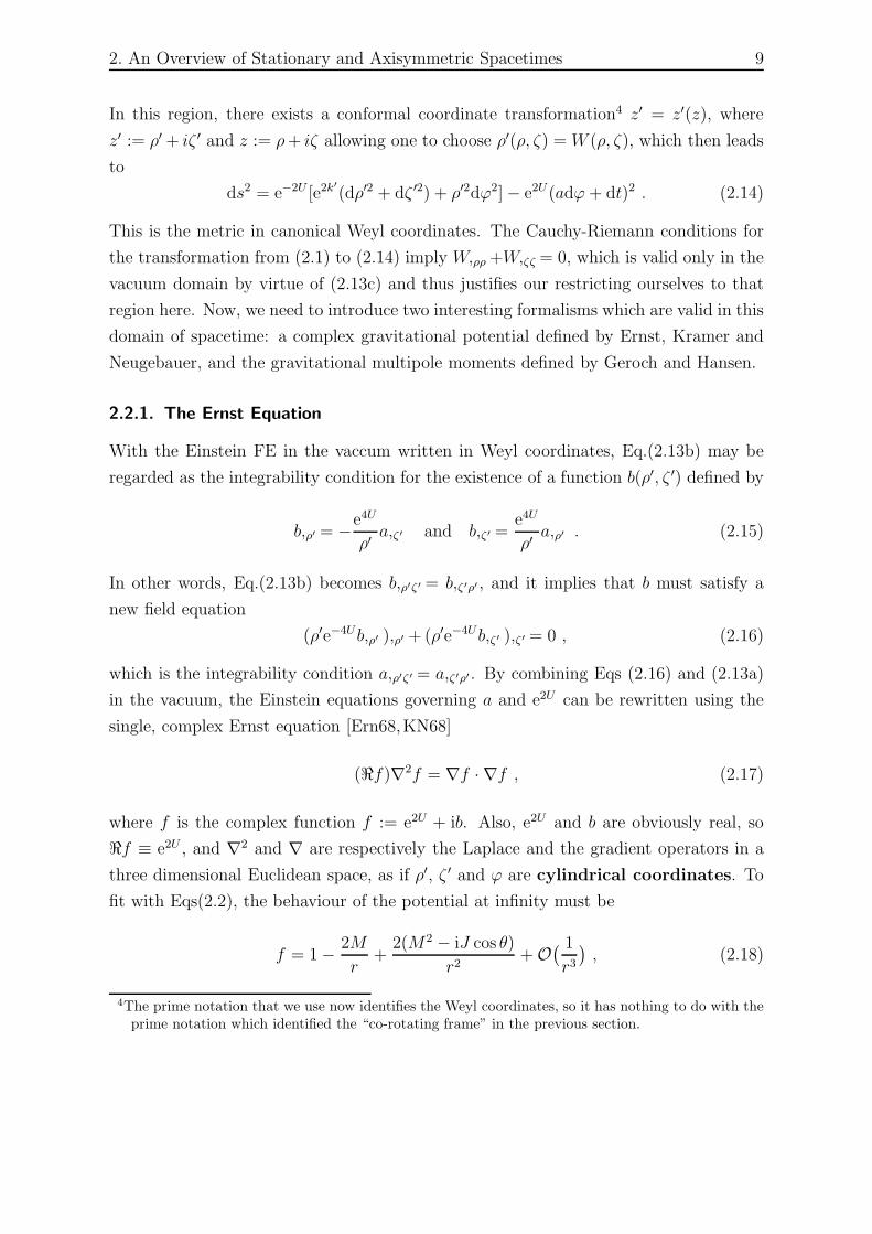
2.2.1. The Ernst Equation
With the Einstein FE in the vaccum written in Weyl coordinates, Eq.(2.13b) may be
regarded as the integrability condition for the existence of a function b(ρ′, ζ ′) defined by
b,ρ′ = −e4U
ρ′a,ζ′ and b,ζ′ =
e4U
ρ′a,ρ′ . (2.15)
In other words, Eq.(2.13b) becomes b,ρ′ζ′ = b,ζ′ρ′ , and it implies that b must satisfy a
new field equation
(ρ′e−4Ub,ρ′ ),ρ′ + (ρ′e−4Ub,ζ′ ),ζ′ = 0 , (2.16)
which is the integrability condition a,ρ′ζ′ = a,ζ′ρ′. By combining Eqs (2.16) and (2.13a)
in the vacuum, the Einstein equations governing a and e2U can be rewritten using the
single, complex Ernst equation [Ern68,KN68]
(ℜf)∇2f = ∇f · ∇f , (2.17)
where f is the complex function f := e2U + ib. Also, e2U and b are obviously real, so
ℜf ≡ e2U , and ∇2 and ∇ are respectively the Laplace and the gradient operators in a
three dimensional Euclidean space, as if ρ′, ζ ′ and ϕ are cylindrical coordinates. To
fit with Eqs(2.2), the behaviour of the potential at infinity must be
f = 1 − 2M
r+
2(M2 − iJ cos θ)
r2+ O
( 1
r3
), (2.18)
4The prime notation that we use now identifies the Weyl coordinates, so it has nothing to do with theprime notation which identified the “co-rotating frame” in the previous section.
2. An Overview of Stationary and Axisymmetric Spacetimes 10
where r :=√
ρ′2 + ζ ′2 and tan θ := ρ′/ζ ′.
Once a and U have been solved for, the metric function k′ can be calculated via a line
integral. Solutions of the Ernst equation lead to solutions of the Einstein equations and
the metric potentials in the vacuum can be calculated from:
a,ρ′ = ρ′e−4Ub,ζ′ (2.19a)
a,ζ′ = −ρ′e−4Ub,ρ′ (2.19b)
k′,ρ′ = ρ′[U,2ρ′ −U,2ζ′ +e−4U
4(b,2ρ′ −b,2ζ′ )] (2.19c)
k′,ζ′ = 2ρ′[U,ρ′ U,ζ′ +e−4U
4b,ρ′ b,ζ′ ]. (2.19d)
Not only the form (2.17) of the Ernst equation is valid in both the “co-rotating” and
“non-rotating” frame, the Laplace and gradient operators can also be used in other
3-dimensional Euclidean coordinate systems.
The Ernst equation is a powerful tool to solve the Einstein field equations of axisym-
metric and stationary spacetimes in the vacuum since once we have a solution for f ,
the whole metric (2.14) can then be systematically determined. On the other hand, this
formalism cannot be extended inside matter, so it is not sufficient to generate global
solutions.
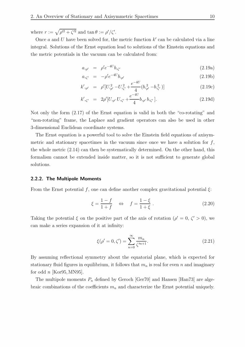
2.2.2. The Multipole Moments
From the Ernst potential f , one can define another complex gravitational potential ξ:
ξ =1 − f
1 + f⇔ f =
1 − ξ
1 + ξ. (2.20)
Taking the potential ξ on the positive part of the axis of rotation (ρ′ = 0, ζ ′ > 0), we
can make a series expansion of it at infinity:
ξ(ρ′ = 0, ζ ′) =
∞∑
n=0
mn
ζ ′n+1. (2.21)
By assuming reflectional symmetry about the equatorial plane, which is expected for
stationary fluid figures in equilibrium, it follows that mn is real for even n and imaginary
for odd n [Kor95,MN95].
The multipole moments Pn defined by Geroch [Ger70] and Hansen [Han73] are alge-
braic combinations of the coefficients mn and characterize the Ernst potential uniquely.
2. An Overview of Stationary and Axisymmetric Spacetimes 11
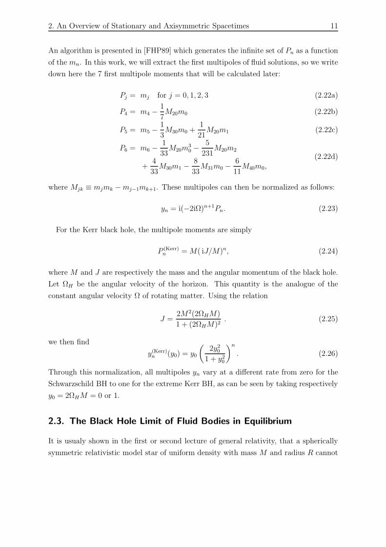
An algorithm is presented in [FHP89] which generates the infinite set of Pn as a function
of the mn. In this work, we will extract the first multipoles of fluid solutions, so we write
down here the 7 first multipole moments that will be calculated later:
Pj = mj for j = 0, 1, 2, 3 (2.22a)
P4 = m4 −1
7M20m0 (2.22b)
P5 = m5 −1
3M30m0 +
1
21M20m1 (2.22c)
P6 = m6 −1
33M20m
30 −
5
231M20m2
+4
33M30m1 −
8
33M31m0 −
6
11M40m0,
(2.22d)
where Mjk ≡ mjmk − mj−1mk+1. These multipoles can then be normalized as follows:
yn = i(−2iΩ)n+1Pn. (2.23)
For the Kerr black hole, the multipole moments are simply
P (Kerr)n = M( iJ/M)n, (2.24)
where M and J are respectively the mass and the angular momentum of the black hole.
Let ΩH be the angular velocity of the horizon. This quantity is the analogue of the
constant angular velocity Ω of rotating matter. Using the relation
J =2M2(2ΩHM)
1 + (2ΩHM)2. (2.25)
we then find
y(Kerr)n (y0) = y0
(2y2
0
1 + y20
)n
. (2.26)
Through this normalization, all multipoles yn vary at a different rate from zero for the
Schwarzschild BH to one for the extreme Kerr BH, as can be seen by taking respectively
y0 = 2ΩHM = 0 or 1.
2.3. The Black Hole Limit of Fluid Bodies in Equilibrium
It is usualy shown in the first or second lecture of general relativity, that a spherically
symmetric relativistic model star of uniform density with mass M and radius R cannot
2. An Overview of Stationary and Axisymmetric Spacetimes 12
be compressed beyond the limit R/RS = 9/8 (RS is the Schwarzschild radius) without
dynamically collapsing, since the pressure in the centre of the body becomes infinite.
The same logic can be extended to a larger class of equations of state for which the
energy density decreases monotonically from the centre of the star to its surface: static
stars can only be in equilibrium for R/RS > 9/8. There is no continuous sequence of
static fluid bodies in equilibrium leading to a black hole.
However, we could ask if a continuous sequence of fluid bodies in equilibrium can
exist for the more general class of stationary and axisymmetric spacetimes. For the
static case, the Tolman-Oppenheimer-Volkoff equation is used to relate the radius of a
star to its pressure in the centre. With such an approach in the rotating case, we would
probably be restricted to searching for a black hole limit through numerical methods for
different rotating star configurations near the infinite pressure limit. Instead, we should
begin by asking what conditions need to be satisfied for a fluid body in equilibrium to
realize in the limit a black hole.
2.3.1. Necessary and Sufficient Condiditions for a Black Hole Limit
The horizon of a black hole can be intuitively described as a hypersurface boundary,
where it becomes impossible for events “inside the boundary” to have time-like or null-
like curves that can reach and influence the future of the domain “outside the boundary”.
The usual mathematical approach to define a horizon is to identify it as a null hyper-
surface, i.e. a hypersurface whose normal at every point is a null vector (nαnα = 0). In
the case of the Kerr BH, the horizon corresponds to the condition e2V = 0 and a normal
vector can be obtained by the gradient
e2V ,α = −2κ(ξα + ΩH ηα) ,
where κ and ΩH are respectively the surface gravity and the angular velocity of the
horizon, related to the mass M and angular momentum J of the black hole by
κ =
√M2 − (J/M)2
2M[M +
√M2 − (J/M)2
] , ΩH =J
2M2[M +
√M2 − (J/M)2
] . (2.27)
Thus, the only linear combination of Killing vectors which does not become space-like
on the horizon of a black hole is a null one:
(ξα + ΩH ηα)(ξα + ΩH ηα) = 0 . (2.28)
2. An Overview of Stationary and Axisymmetric Spacetimes 13
On the other hand, the surface of a fluid body, characterized by the 4-velocity field of
Eq.(2.6) and the constant potential U ′ ≡ V = V0, has the surface condition
(ξα + Ω ηα)(ξα + Ω ηα) = −e2V0 , (2.29)
because the norm of 4-velocities is always uαuα = −1. If a continuous sequence of fluid
figures in equilibrium can reach a black hole limit, it must be a sequence of bodies with
time-like rotating velocity. Then, the surface of the body can only approach the limit
of a BH horizon for Ω = ΩH , the only non-space-like Killing vector combination on
a horizon. Comparing Eqs (2.29) and (2.28), we see that a sequence of fluid surfaces
requires V0 → −∞ to approach, in the limit, a horizon surface. We will see now that
this condition puts a constraint on the mass and angular velocity of a fluid body.
From Eqs(2.7), the mass and angular momentum of a rotating fluid are related through
M = 2ΩJ +
∫ǫ + 3p
ǫBeV dMB ,
where we use the short form dMB ≡ ǫB e2k′−3V W dρ dζdϕ. Substituting the baryonic
mass with Eq.(2.9) and using the property h(p)eV = h(0)eV0 , we get
M = 2ΩJ + eV0h(0)
∫ǫ + 3p
ǫ + pdMB .
We can easily see that the integral can range only from MB to 3MB. If we assume that
h(0)MB is always finite, the limit V0 → −∞ gives the constraint
M = 2ΩJ .
The Kerr BH that has a mass and angular momentum such that M = 2ΩHJ is the
extreme Kerr BH, where ΩH = ±1/(2M) and J = ±M2. Since we stated above that
the black hole limit can only be reached for Ω = ΩH , the conclusion from [Mei04] is that
the only possible candidate for a black hole limit of fluid bodies in equilibrium is the
extreme Kerr BH, characterized by J = ±M2.
A question that arises now: does a fluid body with V0 → −∞ necessarily have an event
horizon? If we consider the specific energy of Eq.(2.12) for particles of fluid resting on
the surface of the source, with the 4-velocity of Eq.(2.6), it reads
−eV0E = (ξα + Ω ηα)ξα .
2. An Overview of Stationary and Axisymmetric Spacetimes 14
Assuming that particles on the surface are at least marginally bound (E ≤ 1), the last
equation implies in the limit V0 → −∞ that
(ξα + Ω ηα)ξα → 0 , and thus (ξα + Ω ηα)ηα → 0 .
Thus, the Killing vector (ξα + Ω ηα) becomes orthogonal to ξα and ηα on the surface
of the fluid, and because the Killing vectors ξα and ηα are always orthogonal to sur-
faces of constant (ϕ, t), it can be seen that the vector (ξα + Ω ηα) becomes orthogonal
to three linearly independent tangent vectors at each point of the fluid hypersurface.
Then, (ξα + Ω ηα) is a normal vector at every point of that hypersurface, and because
of Eq.(2.29) and e2V0 = 0, this normal vector is a null vector. The surface of the fluid
corresponds to a null hypersurface and then satisfies the conditions for a horizon. There-
fore, the metric of an extreme Kerr BH results outside the horizon, whenever a sequence
of fluid bodies admits the limit V0 → −∞ [Mei06].
2.3.2. The Extreme Kerr Black Hole Geometry
Because the extreme Kerr solution results in the black hole limit of fluid bodies, some
basic information should be given about it. Some properties of the spacetime are par-
ticular and unique compared to the Kerr solution in general. The extreme Kerr BH is
uniquely characterized by a single physical parameter; it is usual to choose either M , J
or Ω, which are related through:
J = M2 , M = 2ΩJ or 2ΩM = 1. (2.30)
With the spherical-like version of Weyl coordinates r =√
ρ′2 + ζ ′2 and tan θ = ρ′/ζ ′,
the Ernst potential of the extreme Kerr BH reads
f =r/M − 1 − i cos θ
r/M + 1 − i cos θ. (2.31)
The metric can be rewritten using Eqs(2.19), and it takes the form
ds2 = e−2U [e2k(dr2 + r2dθ2) + r2 sin2 θdϕ2] − e2U(adϕ + dt)2 ,
with the following metric potentials:
e2U =r2 − M2 sin2 θ
(r + M)2 + M2 cos2 θ,
2. An Overview of Stationary and Axisymmetric Spacetimes 15
a =2M2(r + M) sin2 θ
r2 − M2 sin2 θ,
e2k =r2 − M2 sin2 θ
r2.
The transformation of the metric into the better known Boyer-Lindquist coordinates can
be achieved using the substitution r = rBL−M , with rBL being Boyer-Lindquist’s radial
coordinate. Note that this last substitution holds only for the extreme Kerr BH; more
complicated transformation relations are needed to link the Weyl-Lewis-Papapetrou co-
ordinates with Boyer-Lindquist coordinates for the whole class of the Kerr solution.
The most particular property of the extreme Kerr BH is certainly its degenerated
horizon. The event horizon of the black hole is the surface where grr goes to infinity,
which occurs here at r = 0, i.e. in a single point at the origin of the coordinate system.
The Weyl coordinates do not show it very well, but the horizon still has a finite area
A = 8πM2 and the point r = 0 contains an infinite 3-dimensional volume, as we can see
by measuring a proper radial distance from the centre
δ(R) =
R∫
0
√grr dr =
R∫
0
√(1 +
M
r
)2
+M2 cos2 θ
r2dr = ∞ (2.32)
for any radial coordinate R outside the origin (R > 0). The geometry at the origin can
be better described by transforming the Weyl coordinates into a new set of coordinates
proposed by Bardeen and Horowitz [BH99]:
r = λr′ , θ = θ′ , ϕ = ϕ′ +t′
2Mλ, t =
t′
λ.
In the limit λ → 0, a new line element reveals a infinitely long “throat geometry” for
the corresponding origin in Weyl coordinates:
ds2 =1 + cos2 θ′
2
[2M2
r′2dr′2 + 2M2dθ′2 − r′2
2M2dt′2]
+4M2 sin2 θ′
1 + cos2 θ′
[dϕ′ +
r′
2M2dt′]2
.
This metric is no longer asymptotically flat at spatial infinity. In the case of fluid
bodies reaching the black hole limit, the throat geometry realizes a separation between
two infinitely distant worlds. At one extremity of the throat, an outside world has the
expected extreme Kerr BH solution, with the throat located near the horizon. At the
other extremity, an inner world contains the source around its centre and has the throat
2. An Overview of Stationary and Axisymmetric Spacetimes 16
geometry at its spatial infinity. It should be noted that the horizon is a feature of
the throat geometry, so the surface of the fluid does not become a horizon. When we
required in 2.3.1 that the body’s surface needs to satisfy the conditions on the horizon,
it was from a typical point of view of the outside world, where it becomes impossible to
distinguish the throat from the source: they are both located at the origin of the Weyl
coordinate system.
Thus, it is possible to fit different solutions with matter in the inner world without
affecting the gravitational field of the outside world, as long as the parameters in (2.30)
are kept constant. It has been found that the inner world can contain matter such as
rings of perfect fluid or a rigidly rotating disk of dust. Moreover, continous sequences of
stationary and axisymmetric solutions exist for these bodies, from the Newtonian limit
to the extreme Kerr-BH limit. These given examples will be the central topics of the
next two chapters.
3. Strange Matter Stars and their Parametric Transition
to a Black Hole
Today, astronomical observations have identified more than a thousand compact objects
thought to be neutron stars, most of them being pulsars. Although there is little doubt
as to their existence, there is still much debate as to the properties of the extremely high
density matter that comprises them. One of the competing models to describe neutron
stars includes strange quark matter: matter that contains a mixture of strange quarks
along with the usual up and down quarks. It is even suggested that strange quark matter
could be more stable than nuclear matter, in which case “neutron stars” could in fact
be mainly composed of a pure quark matter core surrounded by a thin nuclear matter
crust [Web05].
In this chapter, we will consider a stellar model made entirely of strange quark mat-
ter. Solutions are produced by numerical methods. We first produce a class of solutions
with spheroidal topology, then we will look in detail at the parametric transition of
strange matter rings to a black hole. The approach we use to study this transition
differs from those in other papers [NM95,Mei02,AKM03b,FHA05], since we here con-
centrate on the behaviour of multipole moments and on the appearance of a region of
spacetime typical of metrics close to the extreme Kerr limit. The properties of axially
symmetric and stationary strange matter have already been studied for spheroidal con-
figurations [GHL+99], but they have not yet been considered for ring topologies and
their parametric transition to a black hole. Moreover, we include a comparison with the
corresponding transitions of rings governed by other equations of state.
The main results of this chapter were published in [LPA07].
3.1. Model and Method used for Relativistic Strange Stars
3.1.1. Equation of State
Our equation of state is based on the MIT bag model [CJJ+74,CJJT74,FJ84,AFO86].
Under extremely high pressure, the nuclear boundaries of “neutron star” matter may
dissolve to create a phase of a deconfined Fermi gas of quarks, i.e. quarks do not
17
3. Strange Matter Stars and their Parametric Transition to a Black Hole 18
form hadrons anymore. Up (u) and down (d) quarks could convert to other flavours
with the weak interactions in order to reach a state of lower Fermi energy. But if we
consider the mass of each flavour of quarks, only the strange (s) quark (ms ≈ 0.1 GeV)
would be added to the quark population since the others have much larger masses
(mc, mb, mt > 1 GeV) than the chemical potentials involved (∼ 0.3 GeV). Electrons
can also be present in order to keep the star electrically neutral. Chemical equilibrium
between the different fermions is maintained via weak interactions:
d ↔ u + e− + νe , s ↔ u + e− + νe , s + u ↔ d + u . (3.1)
The two first reactions involve neutrino escape which cools down the star to near zero
temperature in comparison to the Fermi energy of the quarks. One obtains from the
weak interactions of Eq.(3.1) the following chemical potential relations:
µu + µe = µd = µs ≡ µ .
In its simplest form, the bag model ignores the strong interaction and assumes the
mass of the three light quark flavours to be zero. The equilibrium configuration of
massless quarks has equal numbers of each flavour. Thus, the quark population becomes
electrically neutral and the electron population vanishes. With all these considerations,
the thermodynamic Landau potential of each flavour reads
Ωq = −µ4
q
4π2for q = u, d, s .
The QCD confinement of the quarks is established by a constant energy density B, the
“bag constant”, which describes the energy difference between the QCD vacuum and
the true vacuum. When summed, the pressures pq and energy densities ǫq of each quark
flavour are related to the total pressure p and total energy density ǫ in the star according
to
ǫ − B =∑
q
ǫq =∑
q
(Ωq − µq
∂Ωq
∂µq
)=
9µ4
4π2,
p + B =∑
q
pq =∑
q
−Ωq =3µ4
4π2.
3. Strange Matter Stars and their Parametric Transition to a Black Hole 19
These two last equations lead to a simple equation of state (EOS):
ǫ − 3p = 4B . (3.2)
One can see that for any pressure, the bag constant maintains the quark gas at finite
density. The limits of the bag correspond in our case to the surface of the star, such that
the star is entirely composed of strange matter. Thus, like the homogeneous EOS, but
unlike polytropic models, the density of strange matter is discontinuous at the surface.
Sometimes, we will compare results of strange quark stars with homogeneous fluids which
has the EOS ǫ = constant.
The bag constant B constitutes a natural unit to normalize most physical quantities
into dimensionless values. A typical estimate of this constant is B = 60 MeV fm−3 =
9.6×1033 J/m3 [GHL+99]. Using the solar mass as a second natural unit (with G = c =
1), this estimate translates to B−1/2 = 76.0 M⊙ (e.g. a star with M = 2 × 10⁻²B−1/2
would mean M = 1.52 M⊙). For the baryonic mass, dimensionless values should be
given by taking into account the specific enthalpy from Eq.(2.9). The enthalpy of our
model is given by
h(0) =E
(uds)0
E(ud)0
which is the ratio between the energy per unit baryon number of strange quark versus
normal matter at zero pressure. A typical estimate for this ratio is h(0) = 0.899, which
leads to(h(0)
√B)−1
= 84.5 M⊙ with the values given here. It is interesting to note
that E(uds)0 < E
(ud)0 suggests that strange quark matter would be the true ground state
of matter at zero pressure.
In the Newtonian limit, the pressure p is low and negligible in comparison to B, so
the EOS takes the form ǫ = constant. Therefore, all the known Newtonian solutions
for homogeneous bodies will be found in the Newtonian limit of the MIT bag model.
If unstable at low pressure, a quark model of matter is not relevant in the Newtonian
limit, but it is taken as a limiting case of our EOS. In the most relativistic equilibrium
configurations, the star can reach either infinite central pressure or infinite redshift on
its surface. This first relativistic limit concerns stars with spheroidal topology, while the
latter corresponds to the extreme Kerr BH limit for a class of stars with ring topology.
3. Strange Matter Stars and their Parametric Transition to a Black Hole 20
3.1.2. The Ansorg-Kleinwachter-Meinel Numerical Method
To generate relativistic solutions of stationary and axially symmetric fluid configura-
tions, we used a numerical method described in [AKM03a]. In the AKM-method, the
entire spacetime is compactified and divided in several domains. Because of stationarity,
axial and equatorial symmetries, only one quadrant of the ρ − ζ half-plane needs to be
represented in the compactification. For a given solution, the metric potentials from
Eq.(2.1) are written, using the proper coordinate mapping of each domain, as a spectral
expansion in the form of Chebyshev polynomials of the first kind. The Chebyshev poly-
nomial must reproduce a numerically accurate solution of Einstein field Eqs(2.13) on a
finite set of discrete grid-points covering the domain and the inter-domain boundaries.
To avoid a “Gibbs phenomenon” on the fluid surface discontinuity, one of the domain
boundaries is chosen to coincide with the surface.
By giving an initial solution, the AKM-method calls iteratively the Newton-Raphson
method in order to simultaneously find the metric potentials of a targeted nearby
fluid configuration which must be a solution of Einstein’s FE on the given grid-points.
Through each iteration, the search is constrained by inter-domain boundary conditions
and regularity conditions on the rotation axis and at spatial infinity. However, the
search has to determine the shape of the fluid surface where the metric potentials and
their first derivatives inside and outside the matter must behave continously through
the boundary. By fixing two independent physical parameters and by choosing a scaling
parameter for the coordinates, it should lead to a unique neighbouring solution. The
solution is finally given in a numerical list of Chebyshev coefficients from which one can
compute the metric potentials.
In our search of new configurations, we use some physical parameters not yet men-
tioned, such as the ratio rp/re of polar to equatorial coordinate radius and a mass-shed
parameter β defined as:
β = −r2e
r2p
d(ζ2s )
d(ρ2)
∣∣∣∣∣ρ=re
= − re
r2p
limρ→re
ζsdζs
dρ
where ζs = ζs(ρ) is the ζ-axis position of the surface as a function of ρ. The mass-
shedding limit (also called Keplerian limit in other texts) is characterized by β = 0, while
the case where β = 1 holds for static solutions and Maclaurin spheroids. Fig. 3.1 shows
an example of a strange star configuration in equilibrium, here at the mass-shedding
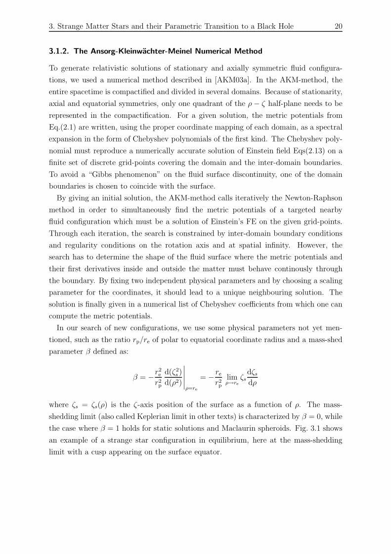
limit with a cusp appearing on the surface equator.
3. Strange Matter Stars and their Parametric Transition to a Black Hole 21
ρ
ζ
re
rp
Figure 3.1: Example of a meridional cross-section of a strange matter star.The star in this example is at the mass-shedding limit, near the maximalgravitational mass configuration of the “Schwarzschild” class, with
√B M =
3.72 × 10⁻².
3.2. Solutions of Strange Quark Matter
3.2.1. The Schwarzchild Class of Strange Quark Matter
For homogeneous stars, it was shown that not all relativistic configurations in equilibrium
are connected continously to each other [SA03, AFK+04]. Starting with a static star
(Ω = 0) with an arbitrary central pressure pc, one can then change the parameters to
find continuous sequences of nearby equilibrium configurations that are bound by
• static solutions (Ω = J = 0 or β = rp/re = 1) with pc ∈ [0,∞],
• stars at infinite central pressure pc = ∞ with β ∈ [0, 1],
• stars at the mass-shedding limit β = 0 with pc ∈ [0,∞],
• Newtonian (non-Maclaurin) flat stars at pc = 0 with β ∈ [0, 1],
• Newtonian Maclaurin spheroids (pc = 0 and β = 1) with rp/re ∈ [0.17126..., 1].
We call it the Schwarzschild class, although it obviously does not contain only static
bodies. It is the class of bodies which contains the most relevant configurations for
astrophysics.
In the case of strange quark matter, we can confirm that a Schwarzschild class exists
with the same five boundaries as for homogeneous stars. Since the Newtonian limit
of strange matter has the same EOS as homogeneous fluids, the two Newtonian limit
sequences (Maclaurin and non-Maclaurin) have in all aspects the same physical char-
acteristics as those of homogeneous fluids with the same constant energy density. But
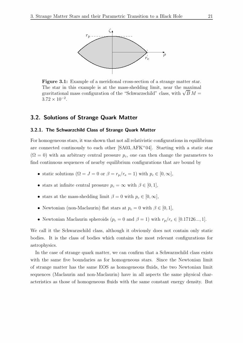
3. Strange Matter Stars and their Parametric Transition to a Black Hole 22
0.0 0.2 0.4 0.6 0.8 1.0
0.01
0.02
0.03
0.04
rp/re
√B M
×
×
×
×× (a)
(b)
(c)
(e) (d)
Figure 3.2: Gravitational mass of the Schwarzschild class for strange matterstars as a function of the flatness (rp/re-ratio). Equilibrium configurations(grey zone) are bounded by sequences of static (a-b), infinite central pressure(b-c), mass-shedding (c-d), non-Maclaurin Newtonian flat stars (d-e) andMaclaurin spheroids (e-a) configurations. The class is folded on the upperright and the dashed line marks the maximal extension of the mass withinthe class.
as the configurations become more relativistic, the behaviour of strange stars differs
significantly.
An important property of strange matter stars is well illustrated by comparing our
Fig. 3.2 with the analogous Fig. 3 in [SA03] for homogeneous density. The Schwarzschild
class of strange matter is such that for typical sequences running from zero pressure to
infinite central pressure, the configuration with maximal mass is one with finite pressure.
In the case of homogeneous stars on the other hand, the mass increases monotonically
as the central pressure increases.
For strange matter, such a sequence of maximal mass dividing the class suggests that
a region of this class might be unstable. Indeed, a test of stability using Eq.(2.11) shows
us that configurations with higher central pressures are unstable. In articles concerning
strange matter stars, the stability with respect to axisymmetric perturbations is usually
illustrated by showing the mass-radius relationship [KWWG95]. This is done here in
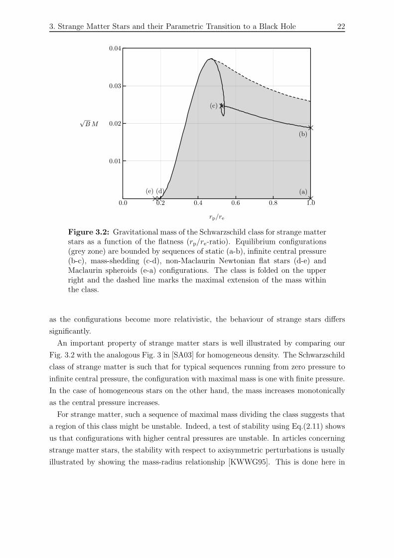
3. Strange Matter Stars and their Parametric Transition to a Black Hole 23
0.00 0.04 0.08 0.12 0.16
0.01
0.02
0.03
0.04
√B Req
√B M
J0
J3
J6
J9
Figure 3.3: Relation between the circumferential radius Req on the equa-tor and the gravitational mass M . Curves of constant angular momentumJ0, J3, J6, J9 are respectively for BJ = 0, 3 × 10⁻⁴, 6 × 10⁻⁴, 9 × 10⁻⁴. Thedots mark maximal masses, the dashed lines are the unstable part of the con-stant J sequences. The dotted line represents the sequence of configurationsat mass-shedding limit and the Newtonian configurations are at origin.
Fig. 3.3, where we plot different sequences of constant angular momentum J . Each
sequence with non-zero angular momentum begins with a relatively low mass along the
mass-shedding limit, then the mass increases until it reaches maximum before decreasing
again. The maximal mass of each sequence marks the limit of stability. On the unstable
side of the sequences, J0 (static) and J3 evolve until the central pressure becomes infinite,
while J6 and J9 are examples of sequences which end again on a mass-shedding limit.
Considering again that a configuration with extremal mass marks a limit of stability
along sequences of constant angular momentum, we can notice in Fig. 3.3 that minima
seem to exist along the mass-shedding limit. By looking more carefully, it appears that
a tiny “valley” of minimal mass exists very near of this limit. Although our numerical
solutions show with confidence these tiny minima inside the class, the resolution was
insufficient to conclude which side of the “valley” should be unstable.
3. Strange Matter Stars and their Parametric Transition to a Black Hole 24
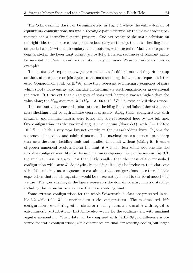
The Schwarzschild class can be summarized in Fig. 3.4 where the entire domain of
equilibrium configurations fits into a rectangle parameterized by the mass-shedding pa-
rameter and a normalized central pressure. One can recognize the static solutions on
the right side, the infinite central pressure boundary on the top, the mass-shedding limit
on the left and Newtonian boundary at the bottom, with the entire Maclaurin sequence
degenerated in the lower right corner (white dot). Different sequences of constant angu-
lar momentum (J-sequences) and constant baryonic mass (N -sequences) are shown as
examples.
The constant N -sequences always start at a mass-shedding limit and they either stop
on the static sequence or join again to the mass-shedding limit. These sequences inter-
ested Gourgoulhon et al. [GHL+99] since they represent evolutionary sequences of stars
which slowly loose energy and angular momentum via electromagnetic or gravitational
radiation. It turns out that a category of stars with baryonic masses higher than the
value along the Ncrit-sequence, h(0)MB = 3.106 × 10⁻² B−1/2, exist only if they rotate.
The constant J-sequences also start at mass-shedding limit and finish either at another
mass-shedding limit or with infinite central pressure. Along them, configurations with
maximal and minimal masses were found and are represented here by the full line.
One configuration has the maximal angular momentum (black dot), with J = 1.226 ×10⁻⁴ B−1, which is very near but not exactly on the mass-shedding limit. It joins the
sequences of maximal and minimal masses. The maximal mass sequence has a sharp
turn near the mass-shedding limit and parallels this limit without joining it. Because
of poorer numerical resolution near the limit, it was not clear which side contains the
unstable configurations, like for the minimal mass sequence. As can be seen in Fig. 3.3,
the minimal mass is always less than 0.1% smaller than the mass of the mass-shed
configuration with same J . So physically speaking, it might be irrelevent to declare one
side of the minimal mass sequence to contain unstable configurations since there is little
expectation that real strange stars would be so accurately bound to this ideal model that
we use. The grey shading in the figure represents the domain of axisymmetric stability
including the inconclusive area near the mass shedding limit.
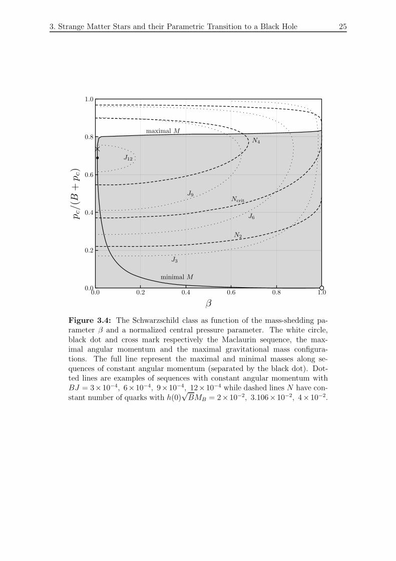
Some extreme configurations for the whole Schwarzschild class are presented in ta-
ble 3.2 while table 3.1 is restricted to static configurations. The maximal red shift
configurations, considering either static or rotating stars, are unstable with regard to
axisymmetric perturbations. Instability also occurs for the configuration with maximal
angular momentum. When data can be compared with [GHL+99], no difference is ob-
served for static configurations, while differences are small for rotating bodies, but larger
3. Strange Matter Stars and their Parametric Transition to a Black Hole 25
0.0 0.2 0.4 0.6 0.8 1.00.0
0.2
0.4
0.6
0.8
1.0
β
pc/(
B+
pc)
maximal M
minimal M
J12
J9
J6
J3
N4
Ncrit
N2
×
Figure 3.4: The Schwarzschild class as function of the mass-shedding pa-rameter β and a normalized central pressure parameter. The white circle,black dot and cross mark respectively the Maclaurin sequence, the max-imal angular momentum and the maximal gravitational mass configura-tions. The full line represent the maximal and minimal masses along se-quences of constant angular momentum (separated by the black dot). Dot-ted lines are examples of sequences with constant angular momentum withBJ = 3×10⁻⁴, 6×10⁻⁴, 9×10⁻⁴, 12×10−4 while dashed lines N have con-stant number of quarks with h(0)
√BMB = 2×10⁻², 3.106×10⁻², 4×10⁻².
3. Strange Matter Stars and their Parametric Transition to a Black Hole 26
Configuration ǫ∗c M∗ M∗B R∗
circ Z0
max. circ. rad. 10.260 2.3653 2.7960 9.9545 0.38041max. mass 19.251 2.5842 3.1061 9.5453 0.47678
max. red shift 42.241 2.4340 2.8802 8.6750 0.50953
Table 3.1: Configurations of static (no rotation) strange stars with max-imal circumferential radius, mass and red shift. The physical quantitiesare as follows: central energy density ǫc = B ǫ∗c , gravitational mass M =0.01B−1/2 M∗, baryonic mass MB = 0.01h(0)−1 B−1/2 M∗
B, circumferentialradius Rcirc = 0.01B−1/2 R∗
circ and red shift Z0.
Configuration rp/re β ǫ∗c M∗ M∗B J∗ Ω∗ Z0
max. flatness 0.1713 1.00 0.000 0.000 0.000 0.000 2.094 0.0000max. ang. moment. 0.4567 0.01 10.64 3.701 4.394 12.26 3.500 0.7775
max. mass 0.4687 0.01 12.37 3.721 4.437 12.13 3.614 0.8177max. pol. red shift 0.5065 0.01 25.27 3.477 4.145 9.841 4.084 0.8895max. ang. velocity 0.5452 0.04 197.6 2.432 2.706 4.202 4.719 0.6882
Table 3.2: Configurations of the entire Schwarzschild class with maximalflatness, angular momentum, mass, polar red shift and angular velocity. Someparameters are the same as in table 3.1 and the others are: polar to equatorradius ratio rp/re, mass shedding parameter β, angular momentum J =10−4B−1J∗, angular velocity Ω =
√B Ω∗ and polar red shift Z0.
than expected considering their accuracy; e.g. our maximal mass is M = 2.828M⊙ and
Gourgoulhon et al. give M = 2.831M⊙ (using B−1/2 = 76.0 M⊙). Although this is
a 0.1% difference for the mass, this configuration from the same authors has a central
density ǫc = 1.261× 10¹⁸ kg m3 while our computation gives ǫc = 1.323× 10¹⁸ kg m3, a
5% difference.
A quark matter model that takes into account the mass of quarks, such as Kettner
et al. [KWWG95], suggests that heavier charm (c) quarks would begin to populate the
matter at energy densities ǫ > 9×1036 J/m3, where the constant B = 57.5 MeV fm−3 =
9.22 × 1033 J/m3 is used. Based on our EOS in Eq.(3.2), such density needs a pressure
beyond B−1 p > 324. With the help of Fig. 3.4, one can identify the stable configuration
with the highest central pressure, which is the most massive static configuration. The
pressure reaches B−1 p = 5.0835, which means that our simple model excludes the
existence of stable stars with heavier quarks than the strange quarks.
The configuration with maximal flatness (table 3.2) lies at a bifurcation point between
Maclaurin spheroids and non-Maclaurin Newtonian stars. This special configuration
connects the Schwarzschild class to a new class of configurations: the ring class. It is
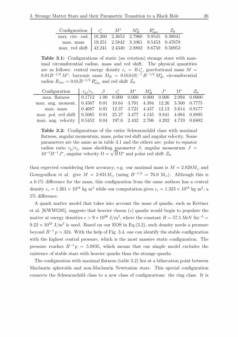
3. Strange Matter Stars and their Parametric Transition to a Black Hole 27
ρi ρo
ρ
ζ
Figure 3.5: Example of a meridional cross-section of a strange matter ring.The ring in this example has the parameters ρi/ρo = 0.7 and e2V0 = 0.1.
the only configuration that allows sequences of strange matter and homogeneous stars in
equilibrium to exit the Schwarzschild class [AFK+04]. No configuration of this first class
has an infinite red shift (the maximum reaches Z0 = 0.8895) and so no star in equilibrium
approaches the black hole limit: only a dynamical collapse can bridge a strange star to
a black hole. On the other hand, the ring class contains figures of equilibrium that reach
the black hole limit, so this class will interest us in the remaining part of this chapter.
3.2.2. The Ring Class of Strange Quark Matter
The ring class includes strange stars that have either spheroidal or toroidal topologies.
The cross-section of a ring is given in Fig. 3.5 as an example. The ratio between the
inner and outer radius ρi/ρo is a parameter of choice to characterize ring configurations.
To represent rings and spheroids consistently, we introduce here a parameter A which
takes the negative value A = −ρi/ρo when it is a ring and the positive value A = rp/re
for spheroids.
Sequences of strange matter bodies are again bound in the same way as for homoge-
neous bodies (see [AFK+04] for details):
• Newtonian “Dyson ring” sequence (V0 = 0) with A ∈ [0.17126...,−1],
• a ring singularity (A = −1) with two possible potentials (V0 = 0 or −∞),
• extreme Kerr black holes (V0 = −∞) containing rings with A ∈ [−1,−0.58428...],
• bodies at the mass-shedding limit (β = 0) with V0 ∈ [−∞, 0],
• Newtonian (non-Maclaurin) flat spheroids at V0 = 0 with β ∈ [0, 1],
• Newtonian Maclaurin spheroids with rp/re ∈ [0.11160..., 0.17126...].
The Newtonian limit of strange matter is always identical to that of homogeneous bodies.
The ring singularity, an infinitely thin ring, is a limiting case where the surface potential
3. Strange Matter Stars and their Parametric Transition to a Black Hole 28
V0 jumps to infinity if the ring is given a non-zero mass. The density of the ring would
jump also to infinity and so, the physical interpretation of such a body is problematic.
The ring singularity should be seen as a limiting case of the ring class and not as a
physically relevant object.
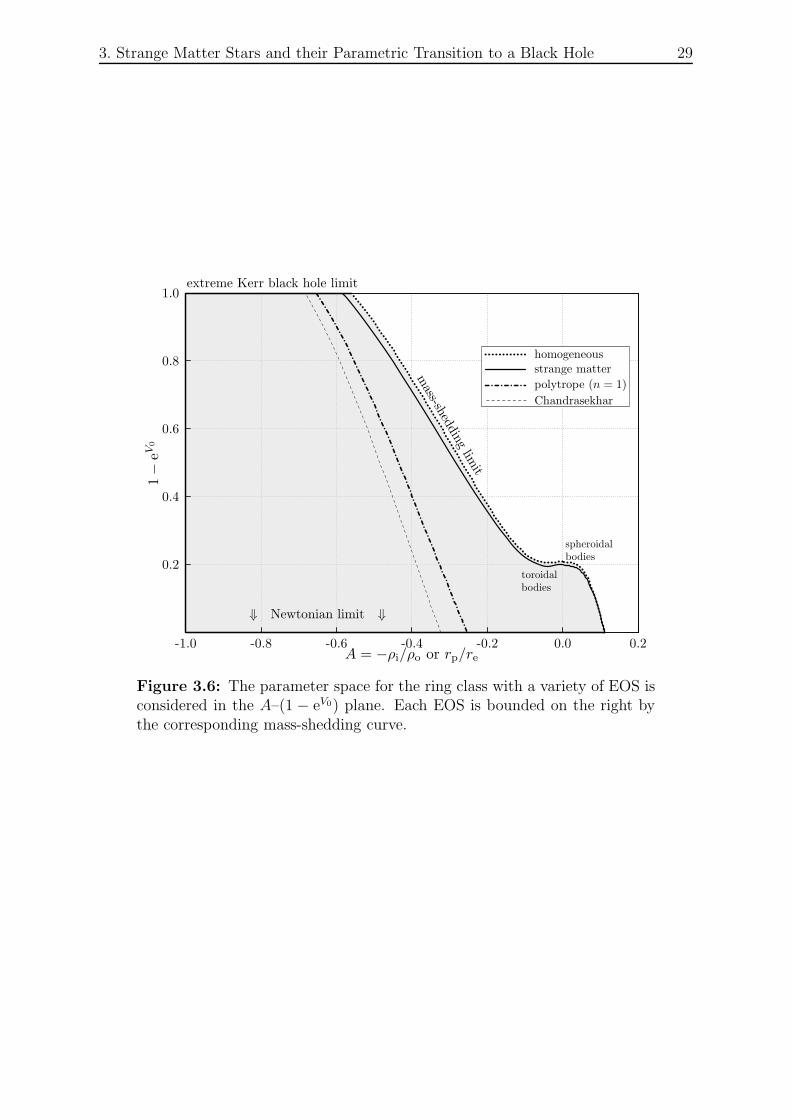
A further comparison of rings of various EOS can be found in Fig. 3.6. Sequences of
rings rotating at the mass-shedding limit, are plotted in a two-dimensional parameter
space with 1 − eV0 on the y-axis and ρi/ρo on the x-axis. The mass-shedding limit is
reached when the path followed by a particle rotating at the outer edge of the ring
becomes a geodesic. For a given EOS, other ring configurations (i.e. not rotating at
the mass-shedding limit) lie to the left of the corresponding curve. One can see that
a transition to the extreme Kerr black hole is a generic feature of all rings considered
here. The transition to spheroidal bodies exists for strange matter rings, but not for
all EOS. What is particularly striking is how close together the curves for strange and
homogeneous rings remain right up to the black hole limit. This figure is a modified
version of Fig. 1 of [FHA05]. A discussion of the polytropic and Chandrasekhar EOS
can also be found in that paper.
3.3. Parametric Transition to a Black Hole
We explained in section 2.3 that the extreme Kerr solution is the only black hole limit of
rotating perfect fluid bodies in equilibrium. The extreme Kerr black hole is characterized
by the relation
J = ±M2,
where M is the mass and J the angular momentum. To study quasi-stationary transi-
tions (sequences of bodies in equilibrium) that lead to black holes, we use bodies with
a ring topology, since spheroidal bodies do not seem to have stationary sequences that
lead to black holes [AFK+04]. For spheroidal bodies, a finite upper bound is observed
for Z0, defined in Eq.(2.8). In contrast, the transition to a black hole occurs if and only if
Z0 → ∞ (see 2.3.1). We will explore now such transitions with the concept of multipole
moments.
3.3.1. Multipole Moments of Rings
The multipole moments that we use were defined in section 2.2.2. As V0 tends to −∞,
we expect the multipole moments to become closer and closer to those of an extreme
Kerr black hole. We tested this numerically by making use of a (slightly modified version
3. Strange Matter Stars and their Parametric Transition to a Black Hole 29
-1.0 -0.8 -0.6 -0.4 -0.2 0.0 0.2
0.2
0.4
0.6
0.8
1.0
A = −ρi/ρo or rp/re
1−
eV0
homogeneousstrange matter
polytrope (n = 1)
Chandrasekhar
mass-shedding
limit
spheroidalbodies
toroidalbodies
extreme Kerr black hole limit
⇓ Newtonian limit ⇓
Figure 3.6: The parameter space for the ring class with a variety of EOS isconsidered in the A–(1 − eV0) plane. Each EOS is bounded on the right bythe corresponding mass-shedding curve.
3. Strange Matter Stars and their Parametric Transition to a Black Hole 30
of a) highly accurate computer program as described in [AKM03a]. This program was
used for all the results presented in this chapter.
The numerical solutions given by the AKM-method are the four potentials corre-
sponding to the metric of Eq.(2.1) inside the body and in the vacuum domain. Since the
multipoles must be read from the Ernst potential, the three potentials U(ζ), a(ζ), W (ζ)
on the ζ-axis in the vacuum must be expressed as two potentials U(ζ ′), a(ζ ′) in the Weyl
coordinate ζ ′ of Eq.(2.14). First, we write the three potentials on the axis as series of ζ
in the form:
limρ→0
e2U = 1 +∞∑
j=1
uj
ζj(3.3a)
limρ→0
a
W 2=
∞∑
j=3
qj
ζj(3.3b)
limρ→0
W
ρ= 1 +
∞∑
j=1
c2j
ζ2j. (3.3c)
By integrating the last equation, one can express ζ on the axis as a function of the Weyl
coordinate ζ ′:
ζ ′ =
∫W
ρdζ = ζ +
∞∑
j=1
c2j
(1 − 2j)ζ2j−1=⇒ ζ = ζ ′ +
∞∑
j=1
c′2j−1
ζ ′ 2j−1.
The Weyl coordinate can be directly introduced into Eq.(3.3a) to find U(ζ ′). Then, the
potential b(ζ ′) can be calculated using all three series from Eqs(3.3), with the help of an
integral from Eq.(2.15) and the property on the axis where a ∝ ρ2 implies a,ρ′ ∝ 2ρ′ :
b(ζ ′) = limρ′→0
∫e4U
ρ′
∂a
∂ρ′dζ ′ = lim
ρ′→02
∫e4U a
W 2dζ ′.
The multipole moments can then be extracted from the Ernst potential f(ζ ′) = e2U(ζ ′)+
ib(ζ ′).
Figures 3.7 and 3.8 show the first seven multipole moments for homogeneous and
strange matter rings where the ratio between the inner coordinate radius ρi and the
outer radius ρo is held constant at a value of ρi/ρo = 0.7. The left side of the plots
corresponds to the Newtonian limit and the right side tends to the black hole limit. As
V0 → −∞, the normalized multipoles all tend to one, demonstrating that this sequence
indeed approaches the extreme Kerr solution.

3. Strange Matter Stars and their Parametric Transition to a Black Hole 31
10−210−110.0
0.2
0.4
0.6
0.8
1.0
eV0
yn
y0
y6
Figure 3.7: The normalized multipoles yn versus eV0 for homogeneous ringswith ρi/ρo = 0.7 .
10−210−110.0
0.2
0.4
0.6
0.8
1.0
eV0
yn
y0
y6
Figure 3.8: The normalized multipoles yn versus eV0 for strange matterrings with ρi/ρo = 0.7.
3. Strange Matter Stars and their Parametric Transition to a Black Hole 32
It is interesting to note, with respect to eV0 (or Z0), how slowly the exterior spacetime
approaches that of a Kerr black hole. Consider, for example, the configuration from
Fig. 3.8 with eV0 = 10−2. Whereas the value J/M2 = 1.00014 is very close to the
limiting value of one reached in the extreme Kerr limit, the product 2ΩM = 0.9813
deviates rather significantly from it. This makes itself felt particularly for the higher
multipole moments where powers of Ω are in play. The moment y4, for example, has
reached only a value of y4 ≈ 0.91 for this configuration.
To understand better the nature of the transition to the black hole, we compare the
multipole moments of the above strange matter ring sequence with those of the Kerr
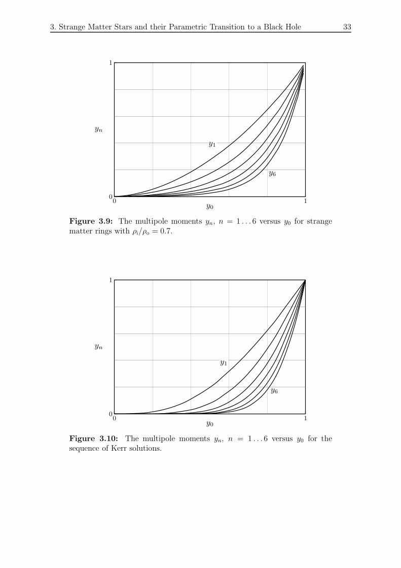
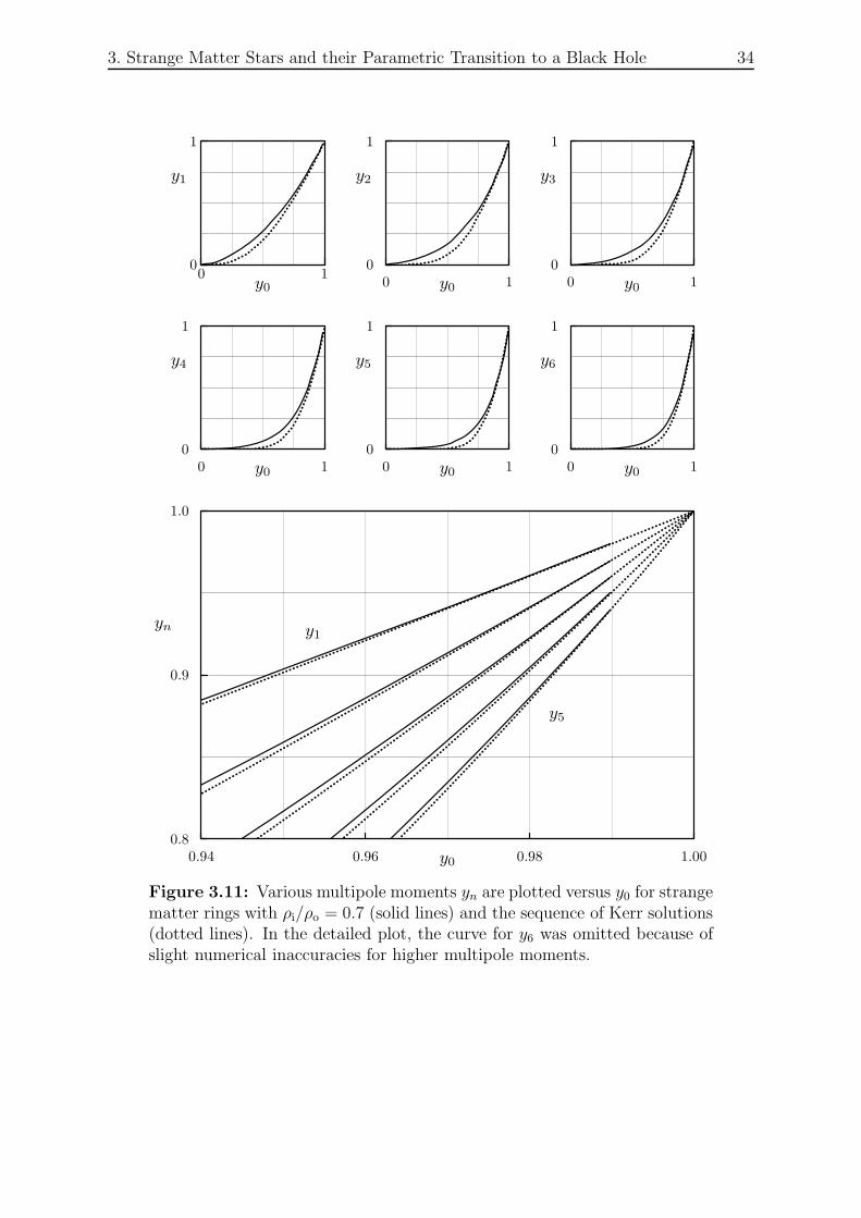
solution. In Fig. 3.9 the yn for n = 1 . . . 6 are plotted against y0 = 2ΩM for the strange
matter ring sequence from above. A corresponding picture for the sequence of Kerr
solutions (see (2.26)) is displayed in Fig. 3.10. The clear similarity between these plots
is emphasized in Fig. 3.11 where each yn for the ring (solid line) and the Kerr solution
(dotted line) is compared in a small figure over its whole range. The region very close
to the extreme Kerr limit is then shown for y1–y5 in detail. The graphs strongly suggest
that the slopesdyn
dy0
(y0 = 1) (3.4)
are the same for the Kerr family and for the strange matter ring sequence discussed
here. In fact, we found these slopes to be independent of the specific EOS being used.1
For the Kerr solutions, it follows from (2.26) that
dyn
dy0(y0 = 1) = n + 1, (3.5)
which leads us to the conjecture that (3.5) holds true for all sequences of rotating bodies
that admit the transition to an extreme Kerr black hole. This conjecture provides a
universal growth rate with which the yn approach unity.
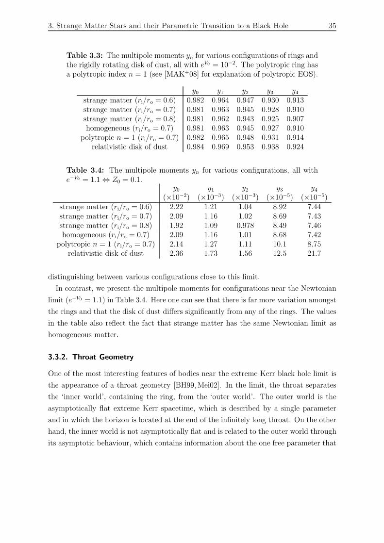
In Table 3.3, a comparison of the values of the first five moments yn for a variety of
configurations all with eV0 = 10−2 is provided. The set of configurations chosen includes
rings with various different EOS and various radius ratios and also includes the uniformly
rotating disk of dust. A discussion of the multipoles of this last configuration as well
as plots analogous to Fig. 3.8 can be found in [KMN95]. Since all multipole moments
tend to one in the limit V0 → −∞, these multipoles will provide almost no way of
1We checked this for ring sequences governed by homogeneous, polytropic and Chandrasekhar EOSas well as for the rigidly rotating dust family (this will be shown for the disk in section 4.3.3). TheChandrasekhar EOS describes a completely degenerate, zero temperature, relativistic Fermi gas.
3. Strange Matter Stars and their Parametric Transition to a Black Hole 33
0 10
1
y0
yn
y1
y6
Figure 3.9: The multipole moments yn, n = 1 . . . 6 versus y0 for strangematter rings with ρi/ρo = 0.7.
0 10
1
y0
yn
y1
y6
Figure 3.10: The multipole moments yn, n = 1 . . . 6 versus y0 for thesequence of Kerr solutions.
3. Strange Matter Stars and their Parametric Transition to a Black Hole 34
0 10
1
y0
y1
0 10
1
y0
y2
0 10
1
y0
y3
0 10
1
y0
y4
0 10
1
y0
y5
0 10
1
y0
y6
0.94 0.96 0.98 1.000.8
0.9
1.0
y0
yn y1
y5
Figure 3.11: Various multipole moments yn are plotted versus y0 for strangematter rings with ρi/ρo = 0.7 (solid lines) and the sequence of Kerr solutions(dotted lines). In the detailed plot, the curve for y6 was omitted because ofslight numerical inaccuracies for higher multipole moments.
3. Strange Matter Stars and their Parametric Transition to a Black Hole 35
Table 3.3: The multipole moments yn for various configurations of rings andthe rigidly rotating disk of dust, all with eV0 = 10−2. The polytropic ring hasa polytropic index n = 1 (see [MAK+08] for explanation of polytropic EOS).
y0 y1 y2 y3 y4
strange matter (ri/ro = 0.6) 0.982 0.964 0.947 0.930 0.913strange matter (ri/ro = 0.7) 0.981 0.963 0.945 0.928 0.910strange matter (ri/ro = 0.8) 0.981 0.962 0.943 0.925 0.907homogeneous (ri/ro = 0.7) 0.981 0.963 0.945 0.927 0.910
polytropic n = 1 (ri/ro = 0.7) 0.982 0.965 0.948 0.931 0.914relativistic disk of dust 0.984 0.969 0.953 0.938 0.924
Table 3.4: The multipole moments yn for various configurations, all withe−V0 = 1.1 ⇔ Z0 = 0.1.
y0 y1 y2 y3 y4
(×10−2) (×10−3) (×10−3) (×10−5) (×10−5)strange matter (ri/ro = 0.6) 2.22 1.21 1.04 8.92 7.44strange matter (ri/ro = 0.7) 2.09 1.16 1.02 8.69 7.43strange matter (ri/ro = 0.8) 1.92 1.09 0.978 8.49 7.46homogeneous (ri/ro = 0.7) 2.09 1.16 1.01 8.68 7.42
polytropic n = 1 (ri/ro = 0.7) 2.14 1.27 1.11 10.1 8.75relativistic disk of dust 2.36 1.73 1.56 12.5 21.7
distinguishing between various configurations close to this limit.
In contrast, we present the multipole moments for configurations near the Newtonian
limit (e−V0 = 1.1) in Table 3.4. Here one can see that there is far more variation amongst
the rings and that the disk of dust differs significantly from any of the rings. The values
in the table also reflect the fact that strange matter has the same Newtonian limit as
homogeneous matter.
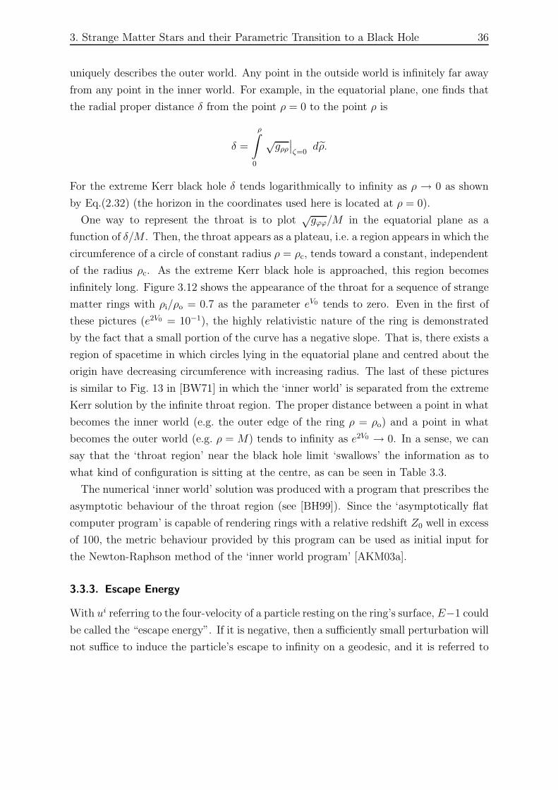
3.3.2. Throat Geometry
One of the most interesting features of bodies near the extreme Kerr black hole limit is
the appearance of a throat geometry [BH99,Mei02]. In the limit, the throat separates
the ‘inner world’, containing the ring, from the ‘outer world’. The outer world is the
asymptotically flat extreme Kerr spacetime, which is described by a single parameter
and in which the horizon is located at the end of the infinitely long throat. On the other
hand, the inner world is not asymptotically flat and is related to the outer world through
its asymptotic behaviour, which contains information about the one free parameter that
3. Strange Matter Stars and their Parametric Transition to a Black Hole 36
uniquely describes the outer world. Any point in the outside world is infinitely far away
from any point in the inner world. For example, in the equatorial plane, one finds that
the radial proper distance δ from the point ρ = 0 to the point ρ is
δ =
ρ∫
0
√gρρ
∣∣ζ=0
dρ.
For the extreme Kerr black hole δ tends logarithmically to infinity as ρ → 0 as shown
by Eq.(2.32) (the horizon in the coordinates used here is located at ρ = 0).
One way to represent the throat is to plot√
gϕϕ/M in the equatorial plane as a
function of δ/M . Then, the throat appears as a plateau, i.e. a region appears in which the
circumference of a circle of constant radius ρ = ρc, tends toward a constant, independent
of the radius ρc. As the extreme Kerr black hole is approached, this region becomes
infinitely long. Figure 3.12 shows the appearance of the throat for a sequence of strange
matter rings with ρi/ρo = 0.7 as the parameter eV0 tends to zero. Even in the first of
these pictures (e2V0 = 10−1), the highly relativistic nature of the ring is demonstrated
by the fact that a small portion of the curve has a negative slope. That is, there exists a
region of spacetime in which circles lying in the equatorial plane and centred about the
origin have decreasing circumference with increasing radius. The last of these pictures
is similar to Fig. 13 in [BW71] in which the ‘inner world’ is separated from the extreme
Kerr solution by the infinite throat region. The proper distance between a point in what
becomes the inner world (e.g. the outer edge of the ring ρ = ρo) and a point in what
becomes the outer world (e.g. ρ = M) tends to infinity as e2V0 → 0. In a sense, we can
say that the ‘throat region’ near the black hole limit ‘swallows’ the information as to
what kind of configuration is sitting at the centre, as can be seen in Table 3.3.
The numerical ‘inner world’ solution was produced with a program that prescribes the
asymptotic behaviour of the throat region (see [BH99]). Since the ‘asymptotically flat
computer program’ is capable of rendering rings with a relative redshift Z0 well in excess
of 100, the metric behaviour provided by this program can be used as initial input for
the Newton-Raphson method of the ‘inner world program’ [AKM03a].
3.3.3. Escape Energy
With ui referring to the four-velocity of a particle resting on the ring’s surface, E−1 could
be called the “escape energy”. If it is negative, then a sufficiently small perturbation will
not suffice to induce the particle’s escape to infinity on a geodesic, and it is referred to
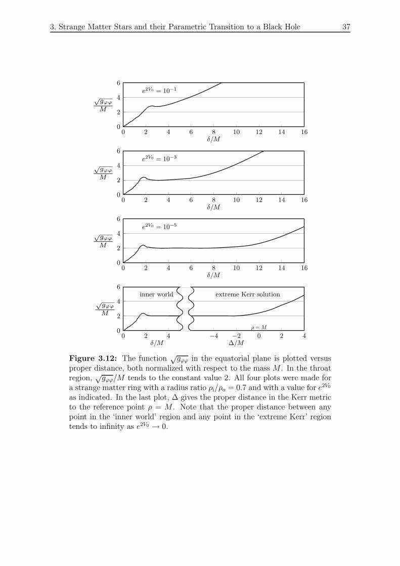
3. Strange Matter Stars and their Parametric Transition to a Black Hole 37
0 2 4 6 8 10 12 14 160
2
4
6
δ/M
√gϕϕ
M
e2V0 = 10−1
0 2 4 6 8 10 12 14 160
2
4
6
δ/M
√gϕϕ
M
e2V0 = 10−3
0 2 4 6 8 10 12 14 160
2
4
6
δ/M
√gϕϕ
M
e2V0 = 10−5
0 2 4 −4 −2 0 2 4
ρ = M0
2
4
6
δ/M ∆/M
√gϕϕ
M
inner world extreme Kerr solution
Figure 3.12: The function√
gϕϕ in the equatorial plane is plotted versusproper distance, both normalized with respect to the mass M . In the throatregion,
√gϕϕ/M tends to the constant value 2. All four plots were made for
a strange matter ring with a radius ratio ρi/ρo = 0.7 and with a value for e2V0
as indicated. In the last plot, ∆ gives the proper distance in the Kerr metricto the reference point ρ = M . Note that the proper distance between anypoint in the ‘inner world’ region and any point in the ‘extreme Kerr’ regiontends to infinity as e2V0 → 0.
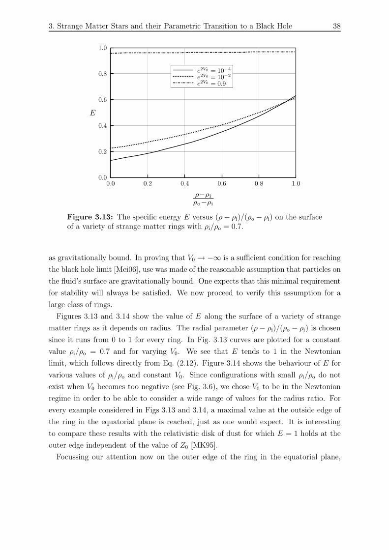
3. Strange Matter Stars and their Parametric Transition to a Black Hole 38
0.0 0.2 0.4 0.6 0.8 1.00.0
0.2
0.4
0.6
0.8
1.0
ρ−ρi
ρo−ρi
E
e2V0 = 10−4
e2V0 = 10−2
e2V0 = 0.9
Figure 3.13: The specific energy E versus (ρ − ρi)/(ρo − ρi) on the surfaceof a variety of strange matter rings with ρi/ρo = 0.7.
as gravitationally bound. In proving that V0 → −∞ is a sufficient condition for reaching
the black hole limit [Mei06], use was made of the reasonable assumption that particles on
the fluid’s surface are gravitationally bound. One expects that this minimal requirement
for stability will always be satisfied. We now proceed to verify this assumption for a
large class of rings.
Figures 3.13 and 3.14 show the value of E along the surface of a variety of strange
matter rings as it depends on radius. The radial parameter (ρ − ρi)/(ρo − ρi) is chosen
since it runs from 0 to 1 for every ring. In Fig. 3.13 curves are plotted for a constant
value ρi/ρo = 0.7 and for varying V0. We see that E tends to 1 in the Newtonian
limit, which follows directly from Eq. (2.12). Figure 3.14 shows the behaviour of E for
various values of ρi/ρo and constant V0. Since configurations with small ρi/ρo do not
exist when V0 becomes too negative (see Fig. 3.6), we chose V0 to be in the Newtonian
regime in order to be able to consider a wide range of values for the radius ratio. For
every example considered in Figs 3.13 and 3.14, a maximal value at the outside edge of
the ring in the equatorial plane is reached, just as one would expect. It is interesting
to compare these results with the relativistic disk of dust for which E = 1 holds at the
outer edge independent of the value of Z0 [MK95].
Focussing our attention now on the outer edge of the ring in the equatorial plane,
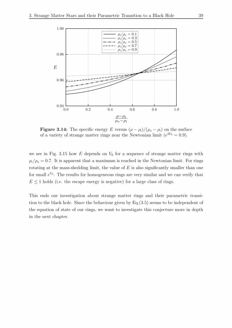
3. Strange Matter Stars and their Parametric Transition to a Black Hole 39
0.0 0.2 0.4 0.6 0.8 1.00.94
0.96
0.98
1.00
ρ−ρi
ρo−ρi
E
ρi/ρo = 0.1ρi/ρo = 0.3ρi/ρo = 0.5ρi/ρo = 0.7ρi/ρo = 0.9
Figure 3.14: The specific energy E versus (ρ − ρi)/(ρo − ρi) on the surfaceof a variety of strange matter rings near the Newtonian limit (e2V0 = 0.9).
we see in Fig. 3.15 how E depends on V0 for a sequence of strange matter rings with
ρi/ρo = 0.7. It is apparent that a maximum is reached in the Newtonian limit. For rings
rotating at the mass-shedding limit, the value of E is also significantly smaller than one
for small eV0 . The results for homogeneous rings are very similar and we can verify that
E ≤ 1 holds (i.e. the escape energy is negative) for a large class of rings.
This ends our investigation about strange matter rings and their parametric transi-
tion to the black hole. Since the behaviour given by Eq.(3.5) seems to be independent of
the equation of state of our rings, we want to investigate this conjecture more in depth
in the next chapter.
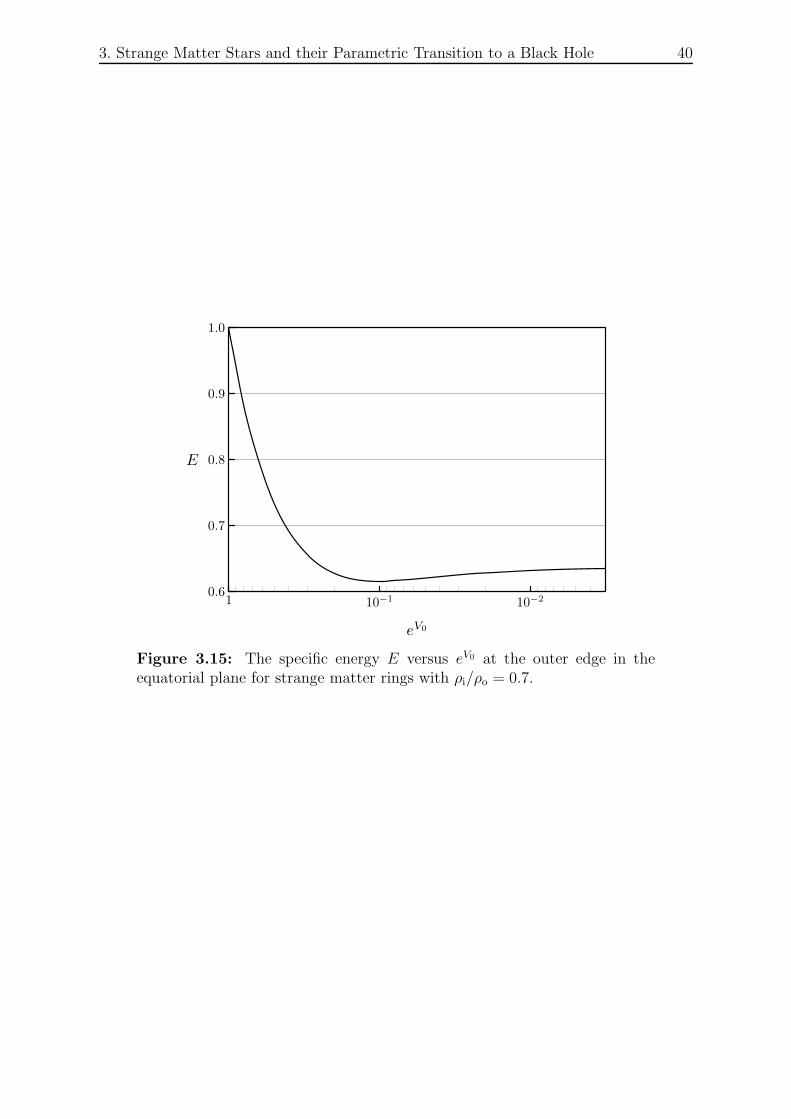
3. Strange Matter Stars and their Parametric Transition to a Black Hole 40
10−210−110.6
0.7
0.8
0.9
1.0
eV0
E
Figure 3.15: The specific energy E versus eV0 at the outer edge in theequatorial plane for strange matter rings with ρi/ρo = 0.7.
4. Ernst Potentials near the Black Hole Limit
Among stationary and axisymmetric solutions containing a black hole or a fluid in equi-
librium as the source, three categories of continuous sequences of solutions are known
to reach the extreme Kerr BH: various rings of fluids [AKM03b, FHA05], the rigidly
rotating disk of dust [BW71,NM93], and obviously, the Kerr BH sequence. Sequences
of rings made of strange quark matter were studied in the previous chapter, and similar
sequences of rings with other equation of states were also produced in the literature
mentioned just above. For the rigidly rotating disk of dust and the Kerr BH, exact
analytical solutions are known.
In the previous chapter, we observed that the multipole moments on the rotation axis
of the rings and the Kerr black hole have a common behaviour near the extreme Kerr
black hole limit, a behaviour characterized by Eq.(3.5). In this chapter, we make use
of (3.5) to write down the beginning of a Taylor series of the Ernst potential of fluids
in equilibrium near the black hole limit, with suitable coordinates. Then, we apply this
Taylor series to the analytical solutions of the Meinel/Neugebauer disk of dust and the
Kerr BH.
4.1. Reformulation of the Conjecture
4.1.1. Normalized Multipoles
Staying in the vacuum domain where we can use of the Weyl coordinates1 and the Ernst
potential, let us first introduce two new pairs of dimensionless Weyl coordinates, one
normalized with the angular velocity Ω of the source, and a second one normalized with
the mass M of the same source:
ρ := 2Ωρ , ζ := 2Ωζ, and (4.1a)
ρ :=ρ
M, ζ :=
ζ
M. (4.1b)
1We drop here the prime notation from section (2.2.1).
41
4. Ernst Potentials near the Black Hole Limit 42
From the potential ξ in Eq.(2.20), one can calculate the same series (2.21) with the
dimensionless coordinates and get the same general form:
ξ =∞∑
n=0
mn
ζn+1=
∞∑
n=0
mn
ζn+1=
∞∑
n=0
mn
ζn+1. (4.2)
The new dimensionless coefficients have the following relations, deduced from (4.2):
mn = (2Ω)n+1mn , mn =mn
Mn+1and mn = (2ΩM)n+1mn . (4.3)
Since the zeroth multipole moment is the gravitational mass of the source, P0 = m0 = M ,
it follows that M = 2ΩM and we can then also say mn = (M)n+1mn. It follows also
that m0 = 1 is an identity.
To avoid becoming lost with the “tilde” and “hat” notation, keep in mind that a
“tilde” is added to a variable when this variable is multiplied by a power of 2Ω such that
it becomes dimensionless, and the same is done with a “hat” when it involves powers
of M to make it dimensionless. The multipole moments can also be transformed into
normalized and dimensionless moments in a similar fashion as the mn coefficients:
Pn = (2Ω)n+1Pn and Pn =Pn
Mn+1(4.4)
These relations seem naively copied from Eq.(4.3) when in fact the Pn for n > 3 are
indeed long algebraic combinations of mn, but a dimensional analysis shows that they
agree.
Because of equatorial symmetry, as stated in section 2.2.2, coefficients and multipoles
with even index are real and the odd ones are purely imaginary. The absolute values
of mn and Pn have a domain going from 0 to 1 for fluid bodies2 and black holes. With
mn and Pn, their absolute values vary from 0 to ∞ for fluid bodies, except for the fixed
number P0 = m0 = 1, while black holes are again restricted to [0,1]. When Pn = 0
for all n, or when Pn = 0 for n > 0, we obtain the Schwarzschild geometry outside the
source, and the scenario where Pn = in or Pn = in for all n corresponds to the extreme
Kerr geometry. More generally, the Kerr black hole has Pn = inMn−1Jn or Pn = inJn,
and it was also found empirically in [FK09] that for a rigidly rotating perfect fluid in
2But only rings and the rigid disk of dust are known to reach 1
4. Ernst Potentials near the Black Hole Limit 43
equilibrium, surrounded by vacuum,
∣∣∣Pn
∣∣∣ ≥∣∣∣Jn∣∣∣ ,
where the right hand side is equivalent to the∣∣∣Pn
∣∣∣ of a Kerr black hole with the same
mass and angular momentum as the fluid body. Also, the equality in this relation is
only reached for the extreme Kerr black hole limit∣∣∣Pn
∣∣∣ = 1.
The normalized multipoles yn defined in Eq.(2.23), which always gives real positive
values for black holes and rings, are related here in this new notation by Pn = inyn. Pn
has the same absolute value as yn, but it is not systematically real positive. This leads
to Pn = mn = in in the extreme Kerr black hole limit, and Eq.(3.5), which we believe
to hold for any sequences of rotating bodies in equilibrium that admit a transition to a
black hole, becomes
dPn
dM(M = 1) =
dmn
dM(M = 1) = (n + 1) in . (4.5)
Note here that the algebraic structure that links Pn and mn is such that choosing Pn or
mn in the derivative of (4.5) is equivalent for M = 1; at least, this is verified for the 11
first multipoles shown in [FHP89], and we are confident that it holds for n > 10.
If we substitute Pn by Pn in the derivative, we get
dPn
dM=
d(Mn+1Pn)
dM= (n + 1)MnPn + Mn+1 dPn
dM.
Putting this last result into Eq.(4.5) with Pn(M = 1) = in, it turns out that the
conjecture takes a nicer form:
dPn
dM(M = 1) =
dmn
dM(M = 1) = 0 . (4.6)
4.1.2. The Multipoles and the First Law of Thermodynamics
It can be shown that a part of our conjecture is indeed explained by the analogous form
of the “first law of thermodynamics” for rotating bodies. In “classical” thermodynamics,
the first law states that for an infinitesimal change in a system of N particles with a
temperature T , an entropy S, a volume V , a pressure p and a chemical potential µc, the
4. Ernst Potentials near the Black Hole Limit 44
internal energy U is changed by
dU = TdS − pdV + µcdN .
When we refer to astrophysical bodies, their physical properties can be also related to
analogous “thermodynamic laws” (or mechanics laws). Nearby configurations between
black holes or between bodies of fluid in equilibrium are governed respectively by the
following “first laws”:
dM = 18π
κ dA + Ω dJ + ∅ ,
dM = ∅ + Ω dJ + µc dMB .
Here, κ is the surface gravity of the black hole, given by Eq.(2.27), and is the black
hole analogue of the temperature. The surface area of the horizon A is analogous to the
entropy. The second equation is from Eq.(2.10). The empty sets (∅) emphasize that black
holes have no “chemical potential-particle” term, while our equation for fluid bodies
shows no “temperature-entropy” term since we consider that our bodies in equilibrium
have zero temperature.
We can see that these laws govern a relation between the two first multipole moments
(M and J). As was explained in section 2.3.1, the parameters κ for black holes and µc
for fluid bodies vanish as they approach the extreme Kerr BH limit. The result is that
the “first law” of both black hole and fluid body configurations become identical in the
limit:
dM = Ω dJ (4.7)
This show that in the extreme Kerr BH limit, not only the mass and angular momentum
is fixed at J = M2, but but the trend of M and J for configurations near this limit is
the same for black holes and fluid bodies.
If we translate the normalized multipoles M , P1 and P1 in terms of M and J and Ω,
we get for infinitesimal changes
dM = d(2ΩM) = 2 (Ω dM + M dΩ) ,
dP1 = d(4iΩ2J) = 4 i (Ω2 dJ + 2 Ω J dΩ) ,
dP1 = d(iM−2J) = i M−2 (dJ − 2 J M−1 dM) .
In the extreme Kerr BH limit, we can subtitute Ω, J and dJ in terms of M and dM
4. Ernst Potentials near the Black Hole Limit 45
thanks to Eqs (2.30) and (4.7). Then we find
dP1
dM(M = 1) =
4i (Ω dM + M dΩ)
2 (Ω dM + M dΩ)= 2i ,
dP1
dM(M = 1) =
0
2 (Ω dM + M dΩ)= 0 .
These results are exactly what is expected in Eqs(4.5) and (4.6) for n = 1. This proves
that what we conjectured for n = 1 is simply a consequence of the first thermodynamic
law for fluid bodies, where its law becomes identical to the black hole thermodynamic
law in the limit of the extreme Kerr BH (2ΩM → 1). No analogous “first law of
thermodynamics” that implies the further multipole moments (n > 1) exists, so we
cannot extend this proof to the entire conjecture.
4.1.3. A Taylor Series Near the Black Hole Limit
Suppose now that we have a list of coefficients mn that can be parameterized as functions
of M . We can thus write the normalized multipoles as a Taylor series at M ≡ 2ΩM → 1
and then use the extreme Kerr black hole result mn(M = 1) = in and the conjecture in
Eq.(4.5) for the two first terms:
mn(M) = mn(1) +dmn
dM(1)(M − 1) +
1
2
d2mn
dM2(1)(M − 1)2 + · · ·
= in[1 + (n + 1)(M − 1) + O[(M − 1)2]
]
It will be more suitable from now on to use the parameter ε := 1−2ΩM , which becomes
ε = 0 in the extreme Kerr black hole limit, and is small and positive near the limit. If
we introduce the last result for the multipoles into Eq.(4.2), we get two sums that can
be substituted into short rational functions:
ξ(ε; ζ) =1
ζ
∞∑
n=0
(i
ζ
)n [1 − (n + 1)ε + O(ε2)
]
=1
ζ
∞∑
n=0
(i
ζ
)n
− 1
ζ
∞∑
n=0
(i
ζ
)n
(n + 1)ε +1
ζ
∞∑
n=0
(i
ζ
)n
O(ε2)
=1
ζ − i− ζ
(ζ − i)2ε + O(ε2) .
4. Ernst Potentials near the Black Hole Limit 46
We can reconstitute from this result the original form of the Ernst potential f using
Eq.(2.20), which yields as a series of ε
f(ε; ζ) =ζ − 1 − i
ζ + 1 − i+
2ζ
(ζ + 1 − i)2ε + O(ε2) . (4.8)
The first part of the series can be easily recognized as the Ernst potential of the extreme
Kerr BH on the ζ-axis. The second part, coming from the conjecture in Eq.(3.5), is
the leading term describing the behaviour of the Ernst potential for a parameterized
transition of a fluid body in equilibrium to the extreme Kerr BH solution. In other
words, the Ernst potential of a black hole and any fluid body in equilibrium with the
same mass M and angular velocity3 Ω, near the limit 2ΩM = 1, have the same Ernst
potential in normalized coordinates on the rotation axis up to O(ε2).
Similar series can be written using the mass as normalization. The Ernst potential is
produced in the same manner as above, and it yields
ξ(ε; ζ) =1
ζ − i+ ∅ + O(ε2) ,
f(ε; ζ) =ζ − 1 − i
ζ + 1 − i+ ∅ + O(ε2) . (4.9)
Again, the extreme Kerr solution occupies the first part of the series, but the next order
correction, corresponding to the conjecture, vanishes (∅). So the Ernst potential on the
axis of a fluid in equilibrium would have sequences of solutions near the extreme Kerr
solution with a first correcting term in O(ε2). The conjecture from Eq.(3.5) or (4.6) is
then equivalent, in normalized Weyl coordinates (ρ, ζ), saying
df
dM(M = 1) = 0 . (4.10)
Moreover, the “extreme Kerr term” in (4.9) already gives the exact mass term 2Mr−1 in
the series expansion at infinity of Eq.(2.18), so the remainder terms O(ε2) of this series
are not expected to contribute in r−1:
ζ − 1 − i
ζ + 1 − i= 1 − 2
ζ+ O
(1
ζ2
)= 1 − 2M
ζ+ O
(1
ζ2
). (4.11)
This is not expected to hold in the former normalization, since the “extreme Kerr term”
3The angular velocity of the horizon in the case of a black hole.
4. Ernst Potentials near the Black Hole Limit 47
in Eq.(4.8) represents a black hole with the same angular momentum as the source of
f , not the same mass.
Using the extreme Kerr black hole as the “anchor” term of a parametric Taylor series
of the Ernst potential near the black hole limit is certainly a relevant choice, since it was
demonstrated in section 2.3 that the extreme Kerr BH is the only candidate for a BH
limit of a stationary and axisymmetric rotating body in equilibrium [Mei06], and such
limits exist for rings and disks of dust. We will turn our work now to two analytically
solved Ernst potentials, the Kerr BH and the the rigidly rotating thin disk of dust,
investigating the property that was conjectured from the rings, and deriving the Taylor
series for these solutions.
4.2. Ernst Potential of the Kerr Black Hole
It is not difficult to make the Taylor series of the Kerr metric, since this metric is not
only already exact, but also, it can be written in a very concise form. Much has been said
about this metric in comparison to other stationary and axisymmetric solutions. The
metric was first found by Kerr [Ker63], then Boyer and Lindquist provided a suitable
coordinate transformation which shed light on the “black hole nature” of the metric
[BL67]. More physical processes concerning rotating black holes were studied, especially
by Bardeen, Press and Teukolsky in [BPT72]; of particular interest in this last article
is the description of the extreme Kerr BH (J = ±M2), with its special infinitely long
“throat geometry”.
Thus, it is not our goal to write down a series expansion for the purpose of investigating
the Kerr solution itself, but instead, it can be used for comparison with other series of
the same kind, and in particular, with the disk of dust in the next section. The Ernst
potential of a Kerr BH of mass M and angular momentum J is
f = 1 − 4M
r− + r+ + 2M + iJ(r− − r+)√
M4 − J2
(4.12)
where r± are positive quantities defined by
r2± = r2
[sin2 θ +
(cos θ ±
√M4 − J2
Mr
)2]
and the coordinates are the “spherical version” of the Weyl coordinates, with ρ = r sin θ
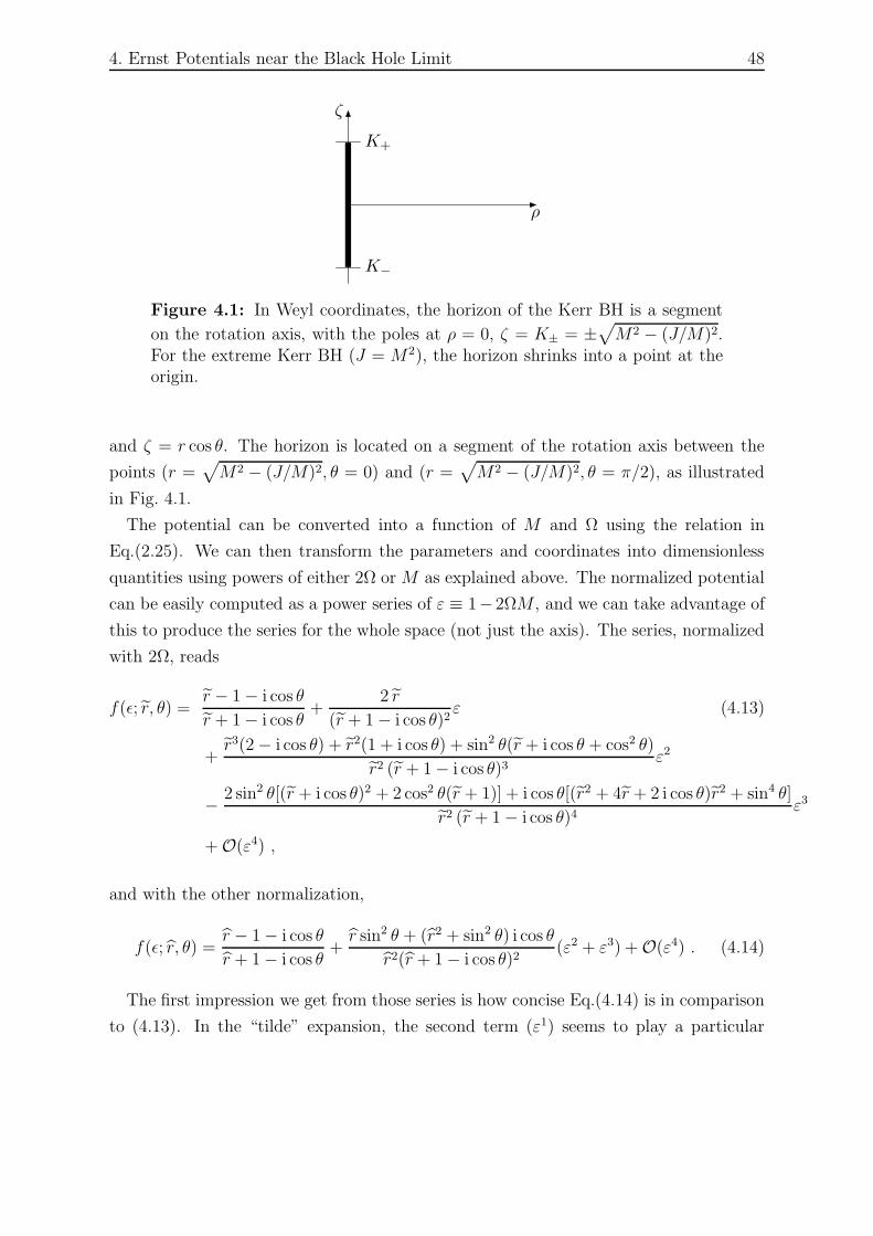
4. Ernst Potentials near the Black Hole Limit 48
K+
K−
ρ
ζ
Figure 4.1: In Weyl coordinates, the horizon of the Kerr BH is a segment
on the rotation axis, with the poles at ρ = 0, ζ = K± = ±√
M2 − (J/M)2.For the extreme Kerr BH (J = M2), the horizon shrinks into a point at theorigin.
and ζ = r cos θ. The horizon is located on a segment of the rotation axis between the
points (r =√
M2 − (J/M)2, θ = 0) and (r =√
M2 − (J/M)2, θ = π/2), as illustrated
in Fig. 4.1.
The potential can be converted into a function of M and Ω using the relation in
Eq.(2.25). We can then transform the parameters and coordinates into dimensionless
quantities using powers of either 2Ω or M as explained above. The normalized potential
can be easily computed as a power series of ε ≡ 1−2ΩM , and we can take advantage of
this to produce the series for the whole space (not just the axis). The series, normalized
with 2Ω, reads
f(ǫ; r, θ) =r − 1 − i cos θ
r + 1 − i cos θ+
2 r
(r + 1 − i cos θ)2ε (4.13)
+r3(2 − i cos θ) + r2(1 + i cos θ) + sin2 θ(r + i cos θ + cos2 θ)
r2 (r + 1 − i cos θ)3ε2
− 2 sin2 θ[(r + i cos θ)2 + 2 cos2 θ(r + 1)] + i cos θ[(r2 + 4r + 2 i cos θ)r2 + sin4 θ]
r2 (r + 1 − i cos θ)4ε3
+ O(ε4) ,
and with the other normalization,
f(ǫ; r, θ) =r − 1 − i cos θ
r + 1 − i cos θ+
r sin2 θ + (r2 + sin2 θ) i cos θ
r2(r + 1 − i cos θ)2(ε2 + ε3) + O(ε4) . (4.14)
The first impression we get from those series is how concise Eq.(4.14) is in comparison
to (4.13). In the “tilde” expansion, the second term (ε1) seems to play a particular
4. Ernst Potentials near the Black Hole Limit 49
function: it introduces the sole correction that the series needs to read the exact mass
of the black hole at spatial infinity. If we expand Eq.(4.13) at r → ∞, we find:
f = 1 − 2(1 − ε)
r+ O
(1
r2
)= 1 − 2M
r+ O
(1
r2
)
Compared with Eq.(4.11) on the axis, we can also say that no further orders of ε are
expected to contribute in r−1 for the black hole.
A second observation concerns the horizon. For the extreme Kerr BH, the horizon
is degenerated to a single point at r = 0. A parametric transition from the extreme
Kerr to the Schwarzschild BH is illustrated in Weyl coordinates by a point-like horizon
becoming a small line on the rotation axis and then growing until its length becomes
2M in the static case (see Fig. 4.1). If we set θ = 0, so we stay on the “positive part”
of the rotation axis, the north pole of the horizon should be met at the point where
e2U ≡ ℜf = 0. In Eq.(4.13), if we consider only the two first terms, we always find
ℜf = 0 at r = r = 0, which suggests that we do not move away from the extreme
Kerr geometry until we consider terms in εn with n > 1, as is obviously the case for
Eq.(4.14).
4.3. Ernst Potential of the Uniformly Rotating Disk of Dust
The Ernst equation simplifies significantly the form of Einstein’s field equations. But
this formalism is restricted to vacuum, and thus, it is insufficent for solving a global
problem where matter fills a part of the spacetime. On the other hand, solving the full
stationary and axisymmetric Einstein field equations with a source is still an arduous
task today, and almost all fully relativistic solutions with matter have been obtained
through numerical methods. Well, not all... If it is possible to model an astrophysical
body where the pressure p vanishes everywhere (also in the body), this would set to zero
the r.h.s. of each equation in (2.13), except (2.13a). Even more, the fact that the r.h.s.
of Eq.(2.13c) becomes zero allows us to adopt the Weyl coordinates (W = ρ) for the
whole spacetime, including inside the body. It is then possible to describe the interior of
the body in the same coordinate system as is needed for the use of the Ernst equation in
empty space. Such a model could be realized if we imagine a uniformly rotating fluid ball
which flattens until it becomes an infinitely thin pressureless fluid disk, more commonly
called the rigidly rotating disk of dust.
The relativistic uniformly rotating disk of dust was already well studied numerically
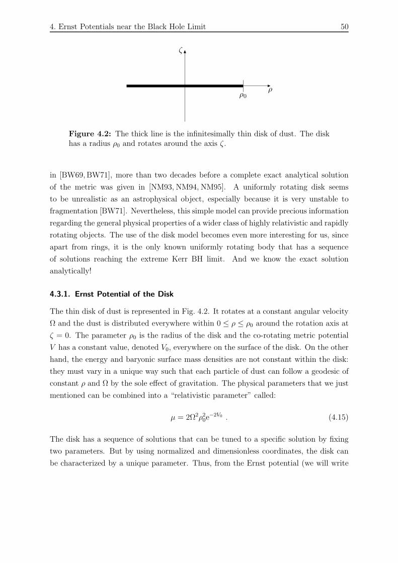
4. Ernst Potentials near the Black Hole Limit 50
ρ0
ρ
ζ
Figure 4.2: The thick line is the infinitesimally thin disk of dust. The diskhas a radius ρ0 and rotates around the axis ζ .
in [BW69,BW71], more than two decades before a complete exact analytical solution
of the metric was given in [NM93, NM94, NM95]. A uniformly rotating disk seems
to be unrealistic as an astrophysical object, especially because it is very unstable to
fragmentation [BW71]. Nevertheless, this simple model can provide precious information
regarding the general physical properties of a wider class of highly relativistic and rapidly
rotating objects. The use of the disk model becomes even more interesting for us, since
apart from rings, it is the only known uniformly rotating body that has a sequence
of solutions reaching the extreme Kerr BH limit. And we know the exact solution
analytically!
4.3.1. Ernst Potential of the Disk
The thin disk of dust is represented in Fig. 4.2. It rotates at a constant angular velocity
Ω and the dust is distributed everywhere within 0 ≤ ρ ≤ ρ0 around the rotation axis at
ζ = 0. The parameter ρ0 is the radius of the disk and the co-rotating metric potential
V has a constant value, denoted V0, everywhere on the surface of the disk. On the other
hand, the energy and baryonic surface mass densities are not constant within the disk:
they must vary in a unique way such that each particle of dust can follow a geodesic of
constant ρ and Ω by the sole effect of gravitation. The physical parameters that we just
mentioned can be combined into a “relativistic parameter” called:
µ = 2Ω2ρ20e
−2V0 . (4.15)
The disk has a sequence of solutions that can be tuned to a specific solution by fixing
two parameters. But by using normalized and dimensionless coordinates, the disk can
be characterized by a unique parameter. Thus, from the Ernst potential (we will write
4. Ernst Potentials near the Black Hole Limit 51
it soon), we can extract dimensionless combinations of physical parameters as functions
of only µ. If we consider also the gravitational mass M and the imaginary part of the
Ernst potential at the centre of the disk b0, we have the following relations
e2V0 =h′cn(I, h′)2
h, b0 = −sn(I, h′) dn(I, h′)
h, (4.16a)
Ω0 ≡ Ωρ0 =1
2
√1 − h′2
h2cn(I, h′) , (4.16b)
M ≡ 2ΩM = − b0 − Ω0c1 , (4.16c)
where am(u, k), sn(u, k), cn(u, k) and dn(u, k) are the Jacobian elliptic functions, and
h, h′, I and c1 are the following functions of µ:4
h =
√1
2
(1 +
1√µ−2 + 1
), h′ =
√1
2
(1 − 1√
µ−2 + 1
), (4.16d)
I =4
√1 + µ2
π
µ∫
0
g(x)√µ − x
dx , g(x) =ln(
√1 + x2 + x)√1 + x2
, (4.16e)
c1 =1õ
2 4
√1 + µ2 E(am(I, h′), h′) − (µ +
√1 + µ2)I0 + I1
, (4.16f)
and In =1
π
µ∫
0
g(x)xn
√µ − x
dx . (4.16g)
We will make extensive use of elliptic functions from now, so we refer you to the def-
initions and conventions that we use in Appendix A. To make our equations easier to
read, we will not specify the argument and modulus of the Jacobian elliptic functions
when they mean 5:
am ≡ am(I, h′), sn ≡ sn(I, h′), cn ≡ cn(I, h′), dn ≡ dn(I, h′). (4.16h)
The Ernst potential for a uniformly rotating disk of dust is given in [NM95] for the
whole spacetime. The form given there uses integrals that need to follow particular
paths on a Riemann surface, but it is possible to rewrite it in the form of Rosenhain’s
4We need to introduce here a function called I with a “hat”, but this “hat” (written a little bit smaller),is not related to our normalization notation (written with a bigger “hat”). We prefer to write it likethis to stay consistent with the notation used in other works in Jena, and hope it will not lead toconfusion.
5Notice italic vs roman fonts to distinguish
4. Ernst Potentials near the Black Hole Limit 52
theta function where it is not necessary to consider the Riemann surface anymore. We
could decide to face up to this full form of the potential and compute the derivatives that
interest us, but although the disk of dust is considered a simple model, its associated
Ernst potential is lengthy and complicated. Since the multipole moments of stationary
and axisymmetric configurations can be entirely obtained from the axis potential, and
thus all information of the gravitation in the vacuum domain can be derived from the
axis potential, it is sufficient to restrict ourselves to the rotation axis, where the potential
becomes simpler. The representation of the potential that we will use is considerably
different form the one given in [NM95], but the transformations are provided in detail
in [MAK+08] (as well as other interesting information concerning the disk solution).
To make the Ernst potential of the disk a function of one physical parameter, in our
case µ, we begin by introducing the normalized and dimensionless coordinates x := ρ/ρ0
and y := ζ/ρ0. The potential on the axis is obtained by evaluating it in the limit x → 0;
it then becomes a function of two variables: f(µ; x = 0, y) → f(µ; y). By restricting
ourselves to the positive part of the axis (y > 0), the Ernst potential can be written as
follows:
f(µ; y) =1 − iNQ−
N + iQ+, (4.17a)
with the following functions defined as real functions of µ and y:
Q± =1 − 2Ω2
0(y2 + 1 +
√(y2 + 1)2 + µ−2)
−b0 ∓ 2Ω0y, (4.17b)
N = expR − 2I(S + V + Z + U) + T
, (4.17c)
R =y√
µ
π√
(y2 + 1)2 + µ−2
µ∫
0
x(y2 + 1) + µ−1
µ(y2 + 1) − x· g(x)√
µ − xdx , (4.17d)
S =h′(y2 − τ 2)
2√
(y2 + 1)2 + µ−2, (4.17e)
V = sign(y − τ)h√
P (1 − hP )(P − h)
1 − hP − h′, (4.17f)
Z = X − E(h′)
K(h′)Y , (4.17g)
U =π
4K(h)
(2Y
K(h′)− 1
), (4.17h)
T = ln ϑ2
(W+ ,−π
K(h′)
K(h)
)− ln ϑ2
(W− ,−π
K(h′)
K(h)
), (4.17i)
4. Ernst Potentials near the Black Hole Limit 53
W± =π
2K(h)
[I ±
(Y − K(h′)
2
)], (4.17j)
X = sign(y − τ)E(υ, h′) , (4.17k)
Y = sign(y − τ)F (υ, h′) , (4.17l)
υ = arcsin
[√1 − hP
h′
], (4.17m)
P =
√(y2 + 1)2 + µ−2 + 2hτy
(y + τ)2(4.17n)
and all the other functions (also real) depend on µ only, namely the Eqs(4.16) and
τ = 4
√µ−2 + 1 .
The function Z is a Jacobian Zeta function like the general form given in Eq.(A.9), and
ϑ2 is the Jacobian theta function given in Eqs(A.10).
The disk solution is physically relevant between the Newtonian limit given by µ → 0
and the ultra-relativistic limit, the black hole limit, given by the smallest positive value
of µ for which cn(I, h′) = 0. This “upper limit”, called µ0, is:
0 ≤ µ ≤ µ0 = 4.6296618434743420427...
Because we are interested in the behaviour of the disk near the black hole limit, where
2ΩM → 1, we will later need the two normalized coordinates of Eq.(4.1). This can be
achieved by substituting y = y(µ) in the Ernst potential with the help of 2ΩM = M(µ)
and Ωρ0 = Ω0(µ):
y(µ) =ζ
ρ0=
2ΩM
2Ωρ0
ζ
M=
M(µ)
2Ω0(µ)ζ , (4.18a)
y(µ) =ζ
ρ0
=2Ωζ
2Ωρ0
=ζ
2Ω0(µ). (4.18b)
It has the consequence that ζ := ζ/M makes the mass M independent of µ and ζ := 2Ωζ
makes the angular velocity Ω independent of µ.
4.3.2. Ernst Potential of the Disk in the Black Hole Limit
The black hole limit is reached for µ → µ0. But simply calculating f(µ0, y) will not give
us the expected black hole potential of Eq.(2.31) on the axis, because the normalized
4. Ernst Potentials near the Black Hole Limit 54
coordinate y becomes the axis coordinate of the inner world (see section 2.3.2). So the
limit µ → µ0 must be achieved with a second condition that guarantees that we end
up with the axis of the outside world. This is achieved by using the non-normalized
coordinate ζ instead of y, which permits the radius of the disk to shrink to zero, or by
evaluating the functions in the limit y → ∞ along with µ → µ0.
Because of Eq.(4.16b), it is also equivalent to saying that the limit is reached for
Ω0 → 0 or ρ0 → 0 (Ω cannot be zero). If we evaluate all the functions in the black hole
limit, we find
am =π
2, sn = 1 , cn = 0 , dn = h(µ0) , I = K(h′(µ0)) ,
ρ0 = 0 , Ω0 = 0 , b0 = −1 , 2ΩM ≡ M = 1 ,
P = 1 , X =E(h′(µ0)
)+ 1 − h′(µ0)
2, Y =
K(h′(µ0)
)
2,
R = 0 , S =h′(µ0)
2, V =
h(µ0) − h′(µ0) − 1
2, Z =
1 − h(µ0)
2,
S + V + Z = 0 , U = 0 , T = 0
which give all together N = 1, and with the help of 2Ω0y = 2Ωζ and 2ΩM = 1:
Q± = 1 ± 2Ωζ or equivalently Q± = 1 ± ζ
M. (4.19)
Finally, the Ernst potential of the disk from Eq.(4.17a) becomes identical to the po-
tential of the extreme Kerr BH on the axis:
f(µ0; ζ) =ζ − 1 − i
ζ + 1 − ior f(µ0; ζ) =
ζ − 1 − i
ζ + 1 − i. (4.20)
This is again the Ernst potential of the extreme Kerr solution on the axis, and the
solution can be uniquely extended to the whole spacetime by performing a Backlund
transformation, which gives Eq.(2.31).
4.3.3. Derivatives of the Ernst Potential in the Black Hole Limit
The next step would be to verify if the conjecture that we observed for rings is also true
for the disk. In this sense, we want to verify if Eq.(4.10) holds. It can be verified by
computing the derivative of the Ernst potential in the normalized parameter set f(µ; ζ),
or equivalently, by using the non-normalized parameter set f(M, µ; ζ) and keeping the
4. Ernst Potentials near the Black Hole Limit 55
mass M constant for the derivatives. So we would expect, considering M constant,
f ′(M, µ; ζ) ≡ df
dM=
df
dµ
/dM
dµ(4.21)
to vanish in the black hole limit. From the chain rule, the last equation can be decom-
posed into
df
dµ=
−1
N + iQ+
[(f + iQ−)
dN
dµ+ if
dQ+
dµ+ iN
dQ−
dµ
], (4.22a)
dM
dµ= − db0
dµ− c1
dΩ0
dµ− Ω0
dc1
dµ(4.22b)
where we expect in the limit that either the first derivative vanishes or the second one
blows up to infinity.
With the help of derivatives of elliptic functions in appendix A and also with Eqs(B.3),
let us first compute the derivatives for Eq.(4.22b):
db0
dµ= 2h′cn
2h′2sn cn dn +
[1 − 2dn2
][E(am , h′) − h2I +
√1 + µ2
dI
dµ
],
dΩ0
dµ=
h′2cn
2
√1 − h′2
h2
[ 1
µ+
sn2
√1 + µ2
]− h′sn dn
4
√µ−2 + 1
[√1 + µ2
dI
dµ+ E(am , h′) − h2I
],
dc1
dµ=
−I1
2µ3/2+
4
√µ−2 + 1
2
[ I − 2E(am , h′)
µ(1 + µ2)+ 4
dE(am , h′)
dµ− 2
dI
dµ
]
and
dE(am , h′)
dµ=
1√1 + µ2
I sn2
1 + µ2+ h′2
(E(am , h′)cn2 − sn cn dn
)+ dn2 dI
dµ,
dI
dµ=
4
√1 + µ2
2π
2g(µ)√µ
+
µ∫
0
g(µ) − g(x)
(µ − x)3/2dx +
µ
1 + µ2
µ∫
0
g(x)√µ − x
dx
.
For the derivative of I, we used the following substitution to have a regular function,
which avoids the presence of a zero in the denominator:
limx→µ
g(x)√µ − x
−µ∫
0
g(x)
2(µ − x)3/2dx ≡ g(µ)√
µ+
µ∫
0
g(µ) − g(x)
2(µ − x)3/2dx . (4.25)
4. Ernst Potentials near the Black Hole Limit 56
We can now evaluate Eq.(4.22b) in the limit µ → µ0:
dI
dµ= 0.2404694628... ,
E(am , h′) = E(h′) = 1.566360837... ,dE(am , h′)
dµ= 0.2414654076... ,
db0
dµ= 0 ,
dΩ0
dµ=
1
2τ
[h2K(h′) − E(h′)√1 + µ2
− dI
dµ
]= −0.1197970406... ,
dc1
dµ= 0.1263305681...
And we can see now that the derivative of M does not become zero and stays finite:
dM
dµ(µ0) = −c1(µ0)
dΩ0
dµ(µ0) = 0.1256363714... (4.26)
Since (4.22b) stays finite, then we expect Eq.(4.22a) to vanish in the limit.
Most terms in (4.22a) are already known by taking the results in section (4.3.2), so
only the three derivatives of N , Q+ and Q− need extra computations. We first use
Eqs(4.18) to express the Eqs(4.17a) as functions of M , µ and ζ , then we split Q± into
numerator and denominator parts to perform the derivative:
Q± =2M2 − M2(ζ2 + ρ2
0 +√
(ζ2 + ρ20)
2 + µ−2ρ40)
2M(∓Mζ − Mb0)=
QNUM
QDEN ±
,
where M , ρ0 and b0 are functions of µ. The derivative gives:
dQ±
dµ=
1
QDEN ±
[dQNUM
dµ− Q±
dQDEN ±
dµ
], (4.27)
dQNUM
dµ= − 2M
[ζ2 + ρ2
0 +√
(ζ2 + ρ20)
2 + µ−2ρ40
]dM
dµ
− 2M2ρ0
[1 +
ζ2 + (1 + µ−2)ρ20√
(ζ2 + ρ20)
2 + µ−2ρ40
]dρ0
dµ+
M2ρ40
µ3√
(ζ2 + ρ20)
2 + µ−2ρ40
,
dQDEN ±
dµ= 2M(∓ ζ
dM
dµ− M
db0
dµ) ,
4. Ernst Potentials near the Black Hole Limit 57
with the derivatives of M and b0 already calculated and
dρ0
dµ=
2M
M
[dΩ0
dµ− Ω0
M
dM
dµ
]. (4.28)
In the limit µ → µ0 (involving ρ0 → 0), Eqs (4.28) and (4.27) become:
dρ0
dµ(µ0) = 2M
dΩ0
dµ(µ0) ≈ −0.2395940813 M , (4.29)
dQ±
dµ(µ0) = ± dM
dµ(µ0)
ζ
M= ∓c1(µ0)
dΩ0
dµ(µ0)
ζ
M≈ ± 0.1256
ζ
M. (4.30)
The last derivatives that remain are those needed for N :
dN
dµ= N
dR
dµ− 2I
[dS
dµ+
dV
dµ+
dZ
dµ+
dU
dµ
]− 2
dI
dµ
[S + V + Z + U
]+
dT
dµ
. (4.31)
The derivative of R is finite for any value of 0 < µ ≤ µ0, but this becomes evident only
if we use a similar substitution like in Eq.(4.25) to keep all terms regular. The result
yields
dR
dµ=
ζ4 − ρ4
0τ4
ρ0
dρ0
dµ+
(ζ2 + ρ20)
2 − µ−2ρ40
2µ
R
(ζ2 + ρ20)
2 + µ−2ρ40
+ρ0
π√
(ζ2 + ρ20)
2 + µ−2ρ40
(ζ2 + ρ2
0τ4)
g(µ)
ζ+ ζ
õ
µ∫
0
G(x, µ, ζ)dx√µ − x
,
with the integrand function
G(x, µ, ζ) =g(µ)
2(µ − x)
(1 +
ρ20τ
4
ζ2
)+
g(x)
µ(ζ2 + ρ20) − xρ2
0
[2(x + µ−1)ρ0
dρ0
dµ− ρ2
0
µ2
− x(ζ2 + ρ20) + µ−1ρ2
0
2(µ − x)− x(ζ2 + ρ2
0) + µ−1ρ20
µ(ζ2 + ρ20) − xρ2
0
(ζ2 + ρ2
0 − 2(µ − x)ρ0dρ0
dµ
)].
The derivatives for S, V , U and Z give
dS
dµ=
S ρ0
(ζ2 + ρ20)
2 + µ−2ρ40
[ρ3
0
µ3− 2(ζ2 + τ 4ρ2
0)dρ0
dµ
]
− 1√(ζ2 + ρ2
0)2 + µ−2ρ4
0
[h(ζ2 − τ 2ρ2
0)
4(1 + µ2)+ h′τ 2ρ0
(dρ0
dµ− ρ0
2µ(1 + µ2)
)],
dV
dµ= V
h′3h
[2 − hP
1 − hP− h
P − h+
2h(h′P − h)
h′(1 − hP − h′)
]
4. Ernst Potentials near the Black Hole Limit 58
+1
2
dP
dµ
[ 1
P− h
1 − hP+
1
P − h+
2h
1 − hP − h′
],
dZ
dµ=
dX
dµ− E(h′)
K(h′)
dY
dµ− Y√
1 + µ2
[h2 +
E(h′)
K(h′)
(E(h′)
K(h′)− 2h2
)],
dU
dµ=
π
4K(h)
1√1 + µ2
[E(h)
K(h)− h′2 − 2Y
K(h′)
(E(h)
K(h)− E(h′)
K(h′)+
µ√1 + µ2
)]
+2
K(h′)
dY
dµ
,
where the derivatives of X, Y and P are
dY
dµ= sign(ζ − τρ0)
dF (υ, h′)
dµ,
dX
dµ= sign(ζ − τρ0)
dE(υ, h′)
dµ,
dF (υ, h′)
dµ=
1√hP
dυ
dµ+
1√1 + µ2
[h2F (υ, h′) − E(υ, h′) +
√(1 − hP )(1 − h/P )
],
dE(υ, h′)
dµ=
√hP
dυ
dµ+
h2
√1 + µ2
[F (υ, h′) − E(υ, h′)
],
dυ
dµ=
1√h(P − h)
[ −h
2√
1 − hP
(dP
dµ+
h′2P√1 + µ2
)+
h2√
1 − hP√1 + µ2
],
dP
dµ=
1
(ζ + τρ0)2
ρ0√(ζ2 + ρ2
0)2 + µ−2ρ4
0
[2(ζ2 + τ 4ρ2
0)dρ0
dµ− ρ3
0
µ3
]
+ hτρ0ζ[ 1√
1 + µ2− 1
µ
]+ 2hτζ
dρ0
dµ− 2Pτ(ζ + τρ0)
[ −ρ0
2µ(1 + µ2)+
dρ0
dµ
].
Finally, only the derivative of T remains, which is made of theta functions. Later in
this work, we will need an elegant way to produce a series of the theta functions of T . So
we spend some effort on writing the derivative of T in a form which involves functions
that were already familiar or used above and where no theta functions are called anymore.
If we consider in general a function ϑ2(w, B) where w and B are functions of a variable
x, one can obtain with the help of Eq.(A.12), Eq.(A.11) and Heuman’s Lambda function
(A.8) the following result:
d
dxln ϑ2(w, B) = Λ0
dw
dx+
Λ2
0
4+
K2(k)
π2
[dn2(u, k′) − 1 +
E(k)
K(k)
]dB
dx(4.32)
with w =πu
2K(k), B = −π
K(k′)
K(k)and Λ0 ≡ Λ0(am(u, k′), k) .
4. Ernst Potentials near the Black Hole Limit 59
This can be used for the theta functions of T , so we get
dT
dµ= Λ0+
dW+
dµ− Λ0−
dW−
dµ(4.33a)
+
Λ2
0+ − Λ20−
4+
K2(h)
π2
[dn2(u+, h′) − dn2(u−, h′)
] dB
dµ,
dW±
dµ=
π
2K(h)
h′2K(h) − E(h)
K(h)√
1 + µ2u± +
dI
dµ± dY
dµ∓ h2K(h′) − E(h′)
2√
1 + µ2
, (4.33b)
dB
dµ=
π
K(h)√
1 + µ2
[E(h′) − K(h′)
(1 − E(h)
K(h)
)], (4.33c)
with the use of the short forms B ≡ −πK(h′)/K(h), Λ0± ≡ Λ0(am(u±, h′), h) and
u± ≡ I ± (Y − K(h′)/2). The derivative of the Ernst potential with respect to the
relativistic parameter µ for disks of constant mass is now fully known.
Only the derivatives in Eq.(4.31) remain to be evaluated in the black hole limit. First,
we need the following derivatives in the limit µ → µ0:
dP
dµ= 4τ(h − 1)
M
ζ
dΩ0
dµ(µ0) ,
dυ
dµ=
√h[2τ
M
ζ
dΩ0
dµ(µ0) +
h − 1
2√
1 + µ20
],
dY
dµ= +
dF (υ, h′)
dµ= 2τ
M
ζ
dΩ0
dµ(µ0) +
h2K(h′) − E(h′)
2√
1 + µ20
,
dX
dµ= +
dE(υ, h′)
dµ= h
[2τ
M
ζ
dΩ0
dµ(µ0) +
hK(h′) − hE(h′) − h′2
2√
1 + µ20
],
dW±
dµ=
π
2K(h)
K(h′)√1 + µ2
0
(h′2 − E(h)
K(h)
)+
dI
dµ± 2τ
M
ζ
dΩ0
dµ(µ0)
,
Λ0± = Λ0
(π
2, h′(µ0)
)= 1 ,
where τ , h and h′ are obviously evaluated at µ0. Then, the limit µ → µ0 for the
derivatives of R, S, V , Z, U and T gives
dR
dµ=
2I1(µ0)√µ0
M
ζ
dΩ0
dµ(µ0) ,
dS
dµ=
−h
4(1 + µ20)
,
dV
dµ=
h′ + h
4(1 + µ20)
+ 2τh(h − 1)M
ζ
dΩ0
dµ(µ0) ,
dZ
dµ=(h − E(h′)
K(h′)
)2τ
M
ζ
dΩ0
dµ(µ0) −
h′
4(1 + µ20)
,
dU
dµ=
πτ
K(h)K(h′)
M
ζ
dΩ0
dµ(µ0) ,
dT
dµ=
2πτ
K(h)
M
ζ
dΩ0
dµ(µ0) .
4. Ernst Potentials near the Black Hole Limit 60
The identities (B.2) are helpful to simplify the results. Now, we can combine these last
results with the functions evaluated at µ0 in section 4.3.2 to write down the black hole
limit of Eq.(4.31), which becomes:
dN
dµ=
2M
ζ
dΩ0
dµ(µ0)
I1(µ0)√
µ0
− 2τh2K(h′) + 2τE(h′)
.
What is found between the brackets is just c1 evaluated at µ0 (see Eq.(4.16f)). So the
limit can be simply written:
dN
dµ(µ0) =
2M
ζc1(µ0)
dΩ0
dµ(µ0) . (4.34)
We are now able to evaluate the derivative for the Ernst potential, in Eq.(4.22a). With
N(µ0) = 1, Eqs (4.19), (4.20), (4.30) and (4.34), we find the expected result:
df
dµ(µ0) = 0 .
This also means that (4.21) vanishes since the denominator given by (4.26) remains
finite:df
dM(M = 1) = 0 .
4.4. Taylor Series of the Disk
Beyond the single task of verifiying if Eq.(4.10) holds for the disk, we can expand the
Ernst potential of the disk using a Taylor series near the BH limit, written in an explicit
form similar to Eqs(4.8) and (4.9). Since the functions of the disk are all written as
function of µ and ζ , we choose to keep the relativistic parameter (µ−µ0) in the expansions
instead of converting everything into the more universal parameter ε = 1 − 2ΩM .
To realize an explicit form of the Taylor series, we make use of a “computer algebra
system” (i.e. Maple and Mathematica) and we divide the work in two steps. First, we
write down the series of all functions that depend on µ only. Then, we do the same for
the remaining functions which depend on µ and ζ . To perform these calculations, the
technical challenge was to program the series such that the time and memory space of
the computation do not blow up. We present here some technical choices to compute
efficiently and compare the series with the exact functions in the context of physics. For
functions depending on ζ , the computation is done twice with using the two normaliza-
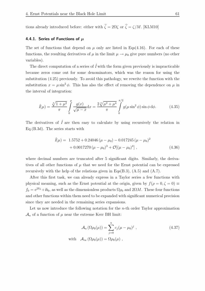
4. Ernst Potentials near the Black Hole Limit 61
tions already introduced before: either with ζ = 2Ωζ or ζ = ζ/M . [KLM10]
4.4.1. Series of Functions of µ
The set of functions that depend on µ only are listed in Eqs(4.16). For each of these
functions, the resulting derivatives of µ in the limit µ → µ0 give pure numbers (no other
variables).
The direct computation of a series of I with the form given previously is impracticable
because zeros come out for some denominators, which was the reason for using the
substitution (4.25) previously. To avoid this pathology, we rewrite the function with the
substitution x = µ sin2 φ. This has also the effect of removing the dependence on µ in
the interval of integration:
I(µ) =4
√1 + µ2
π
µ∫
0
g(x)√µ − x
dx =2 4
√µ2 + µ4
π
π/2∫
0
g(µ sin2 φ) sin φ dφ. (4.35)
The derivatives of I are then easy to calculate by using recursively the relation in
Eq.(B.3d). The series starts with
I(µ) = 1.5752 + 0.24046 (µ− µ0) − 0.017245 (µ− µ0)2
+ 0.0017270 (µ− µ0)3 + O[(µ − µ0)
4] , (4.36)
where decimal numbers are truncated after 5 significant digits. Similarly, the deriva-
tives of all other functions of µ that we need for the Ernst potential can be expressed
recursively with the help of the relations given in Eqs(B.3), (A.5) and (A.7).
After this first task, we can already express in a Taylor series a few functions with
physical meaning, such as the Ernst potential at the origin, given by f(ρ = 0, ζ = 0) ≡f0 = e2V0 +ib0, as well as the dimensionless products Ωρ0 and 2ΩM . These four functions
and other functions within them need to be expanded with significant numerical precision
since they are needed in the remaining series expansions.
Let us now introduce the following notation for the n-th order Taylor approximation
An of a function of µ near the extreme Kerr BH limit:
An (Ωρ0(µ)) =n∑
j=0
cj(µ − µ0)j , (4.37)
with A∞ (Ωρ0(µ)) = Ωρ0(µ) ,
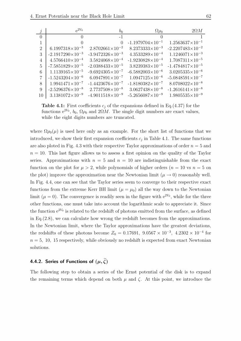
4. Ernst Potentials near the Black Hole Limit 62
j e2V0 b0 Ωρ0 2ΩM0 0 -1 0 11 0 0 -1.1979704×10⁻¹ 1.2563637×10⁻¹
2 6.1997318×10⁻³ 2.8702661×10⁻² 8.2373333×10⁻³ -2.2207483×10⁻²
3 -2.1917290×10⁻³ -3.9472326×10⁻³ 4.3533289×10⁻⁴ 1.1246071×10⁻³
4 4.5766410×10⁻⁴ 3.5824068×10⁻⁴ -1.9230828×10⁻⁴ 1.7087311×10⁻⁵
5 -7.5851829×10⁻⁵ -2.0388433×10⁻⁵ 3.8239383×10⁻⁵ -1.4784817×10⁻⁵
6 1.1139165×10⁻⁵ -9.6924305×10⁻⁷ -6.5882003×10⁻⁶ 3.0205335×10⁻⁶
7 -1.5243204×10⁻⁶ 6.0947891×10⁻⁷ 1.0947125×10⁻⁶ -5.0848591×10⁻⁷
8 1.9941471×10⁻⁷ -1.4423676×10⁻⁷ -1.8180382×10⁻⁷ 8.0708022×10⁻⁸
9 -2.5296376×10⁻⁸ 2.7737508×10⁻⁸ 3.0627438×10⁻⁸ -1.2616141×10⁻⁸
10 3.1381072×10⁻⁹ -4.9011518×10⁻⁹ -5.2656087×10⁻⁹ 1.9805535×10⁻⁹
Table 4.1: First coefficients cj of the expansions defined in Eq.(4.37) for thefunctions e2V0 , b0, Ωρ0 and 2ΩM . The single digit numbers are exact values,while the eight digits numbers are truncated.
where Ωρ0(µ) is used here only as an example. For the short list of functions that we
introduced, we show their first expansion coefficients cj in Table 4.1. The same functions
are also ploted in Fig. 4.3 with their respective Taylor approximations of order n = 5 and
n = 10. This last figure allows us to assess a first opinion on the quality of the Taylor
series. Approximations with n = 5 and n = 10 are indistinguishable from the exact
function on the plot for µ > 2, while polynomials of higher orders (n = 10 vs n = 5 on
the plot) improve the approximation near the Newtonian limit (µ → 0) reasonably well.
In Fig. 4.4, one can see that the Taylor series seem to converge to their respective exact
functions from the extreme Kerr BH limit (µ = µ0) all the way down to the Newtonian
limit (µ = 0). The convergence is readily seen in the figure with e2V0 , while for the three
other functions, one must take into account the logarithmic scale to appreciate it. Since
the function e2V0 is related to the redshift of photons emitted from the surface, as defined
in Eq.(2.8), we can calculate how wrong the redshift becomes from the approximations.
In the Newtonian limit, where the Taylor approximations have the greatest deviations,
the redshifts of these photons become Z0 = 0.17691, 9.0567 × 10⁻³, 4.2302 × 10⁻⁴ for
n = 5, 10, 15 respectively, while obviously no redshift is expected from exact Newtonian
solutions.
4.4.2. Series of Functions of (µ, ζ)
The following step to obtain a series of the Ernst potential of the disk is to expand
the remaining terms which depend on both µ and ζ . At this point, we introduce the
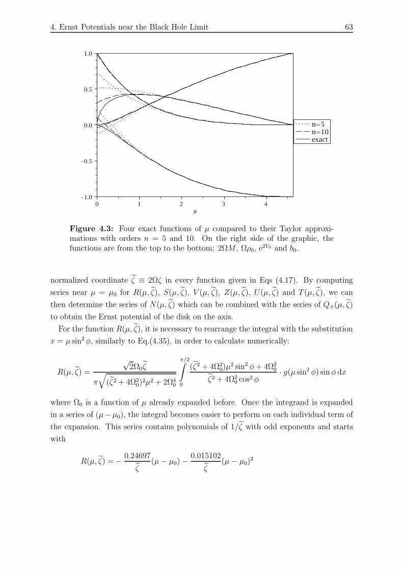
4. Ernst Potentials near the Black Hole Limit 63
n=5n=10exact
m0 1 2 3 4
K1.0
K0.5
0.0
0.5
1.0
Figure 4.3: Four exact functions of µ compared to their Taylor approxi-mations with orders n = 5 and 10. On the right side of the graphic, thefunctions are from the top to the bottom: 2ΩM , Ωρ0, e2V0 and b0.
normalized coordinate ζ ≡ 2Ωζ in every function given in Eqs (4.17). By computing
series near µ = µ0 for R(µ, ζ), S(µ, ζ), V (µ, ζ), Z(µ, ζ), U(µ, ζ) and T (µ, ζ), we can
then determine the series of N(µ, ζ) which can be combined with the series of Q±(µ, ζ)
to obtain the Ernst potential of the disk on the axis.
For the function R(µ, ζ), it is necessary to rearrange the integral with the substitution
x = µ sin2 φ, similarly to Eq.(4.35), in order to calculate numerically:
R(µ, ζ) =
√2Ω0ζ
π
√(ζ2 + 4Ω2
0)2µ2 + 2Ω4
0
π/2∫
0
(ζ2 + 4Ω20)µ
2 sin2 φ + 4Ω20
ζ2 + 4Ω20 cos2 φ
· g(µ sin2 φ) sinφ dx
where Ω0 is a function of µ already expanded before. Once the integrand is expanded
in a series of (µ−µ0), the integral becomes easier to perform on each individual term of
the expansion. This series contains polynomials of 1/ζ with odd exponents and starts
with
R(µ, ζ) = − 0.24697
ζ(µ − µ0) −
0.015102
ζ(µ − µ0)
2
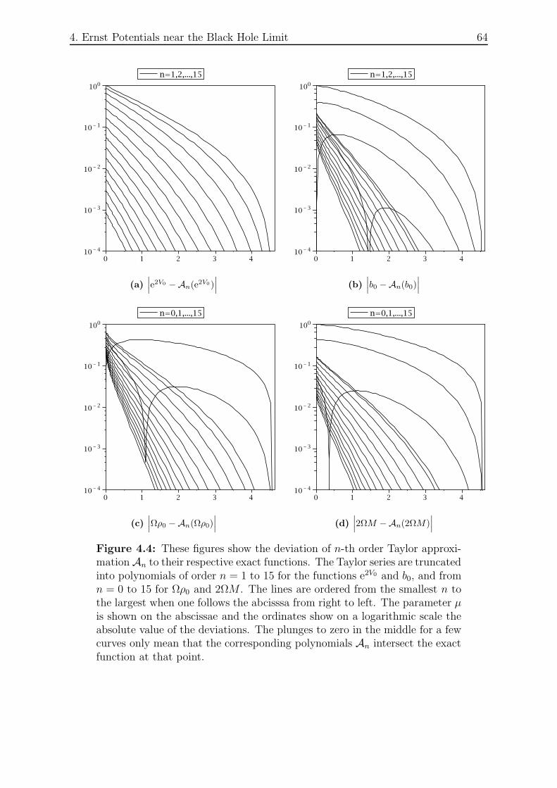
4. Ernst Potentials near the Black Hole Limit 64
n=1,2,...,15
0 1 2 3 4 10 - 4
10 - 3
10 - 2
10 - 1
100
(a)∣∣∣e2V0 −An(e2V0)
∣∣∣
n=1,2,...,15
0 1 2 3 4 10 - 4
10 - 3
10 - 2
10 - 1
100
(b)∣∣∣b0 −An(b0)
∣∣∣
n=0,1,...,15
0 1 2 3 4 10 - 4
10 - 3
10 - 2
10 - 1
100
(c)∣∣∣Ωρ0 −An(Ωρ0)
∣∣∣
n=0,1,...,15
0 1 2 3 4 10 - 4
10 - 3
10 - 2
10 - 1
100
(d)∣∣∣2ΩM −An(2ΩM)
∣∣∣
Figure 4.4: These figures show the deviation of n-th order Taylor approxi-mation An to their respective exact functions. The Taylor series are truncatedinto polynomials of order n = 1 to 15 for the functions e2V0 and b0, and fromn = 0 to 15 for Ωρ0 and 2ΩM . The lines are ordered from the smallest n tothe largest when one follows the abcisssa from right to left. The parameter µis shown on the abscissae and the ordinates show on a logarithmic scale theabsolute value of the deviations. The plunges to zero in the middle for a fewcurves only mean that the corresponding polynomials An intersect the exactfunction at that point.
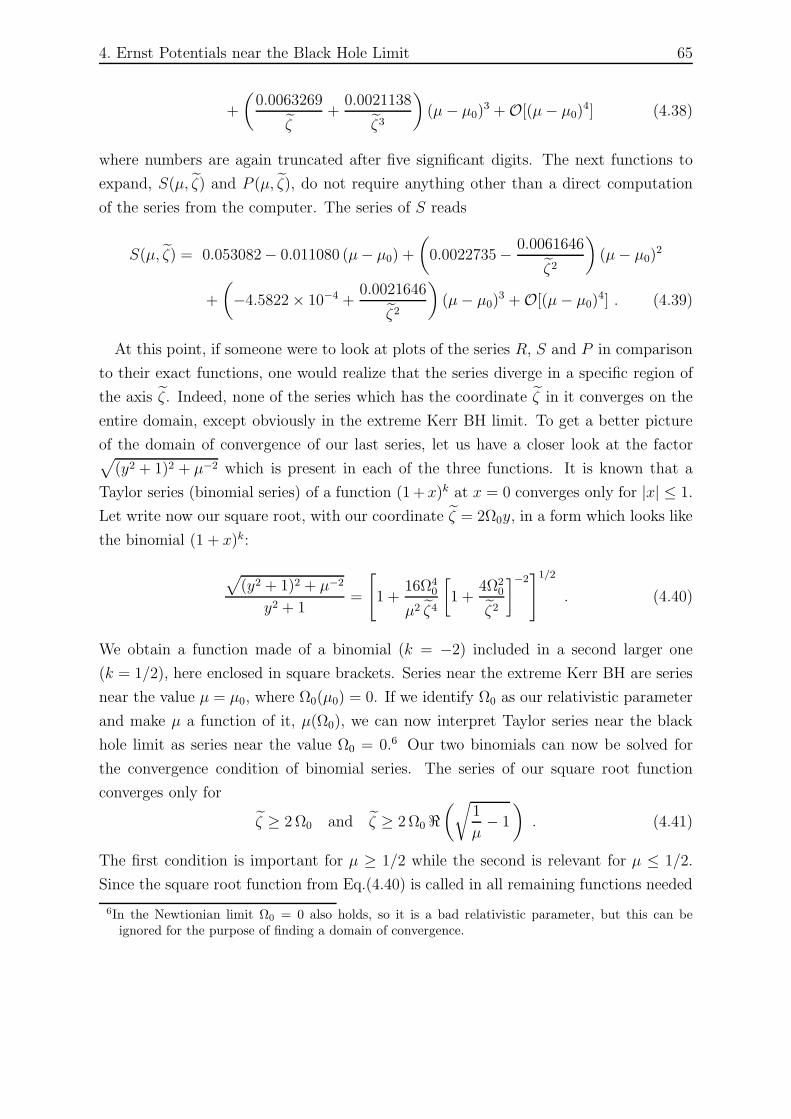
4. Ernst Potentials near the Black Hole Limit 65
+
(0.0063269
ζ+
0.0021138
ζ3
)(µ − µ0)
3 + O[(µ − µ0)4] (4.38)
where numbers are again truncated after five significant digits. The next functions to
expand, S(µ, ζ) and P (µ, ζ), do not require anything other than a direct computation
of the series from the computer. The series of S reads
S(µ, ζ) = 0.053082− 0.011080 (µ− µ0) +
(0.0022735− 0.0061646
ζ2
)(µ − µ0)
2
+
(−4.5822 × 10⁻⁴ +
0.0021646
ζ2
)(µ − µ0)
3 + O[(µ − µ0)4] . (4.39)
At this point, if someone were to look at plots of the series R, S and P in comparison
to their exact functions, one would realize that the series diverge in a specific region of
the axis ζ. Indeed, none of the series which has the coordinate ζ in it converges on the
entire domain, except obviously in the extreme Kerr BH limit. To get a better picture
of the domain of convergence of our last series, let us have a closer look at the factor√(y2 + 1)2 + µ−2 which is present in each of the three functions. It is known that a
Taylor series (binomial series) of a function (1 + x)k at x = 0 converges only for |x| ≤ 1.
Let write now our square root, with our coordinate ζ = 2Ω0y, in a form which looks like
the binomial (1 + x)k:
√(y2 + 1)2 + µ−2
y2 + 1=
[1 +
16Ω40
µ2 ζ4
[1 +
4Ω20
ζ2
]−2]1/2
. (4.40)
We obtain a function made of a binomial (k = −2) included in a second larger one
(k = 1/2), here enclosed in square brackets. Series near the extreme Kerr BH are series
near the value µ = µ0, where Ω0(µ0) = 0. If we identify Ω0 as our relativistic parameter
and make µ a function of it, µ(Ω0), we can now interpret Taylor series near the black
hole limit as series near the value Ω0 = 0.6 Our two binomials can now be solved for
the convergence condition of binomial series. The series of our square root function
converges only for
ζ ≥ 2 Ω0 and ζ ≥ 2 Ω0 ℜ(√
1
µ− 1
). (4.41)
The first condition is important for µ ≥ 1/2 while the second is relevant for µ ≤ 1/2.
Since the square root function from Eq.(4.40) is called in all remaining functions needed
6In the Newtionian limit Ω0 = 0 also holds, so it is a bad relativistic parameter, but this can beignored for the purpose of finding a domain of convergence.
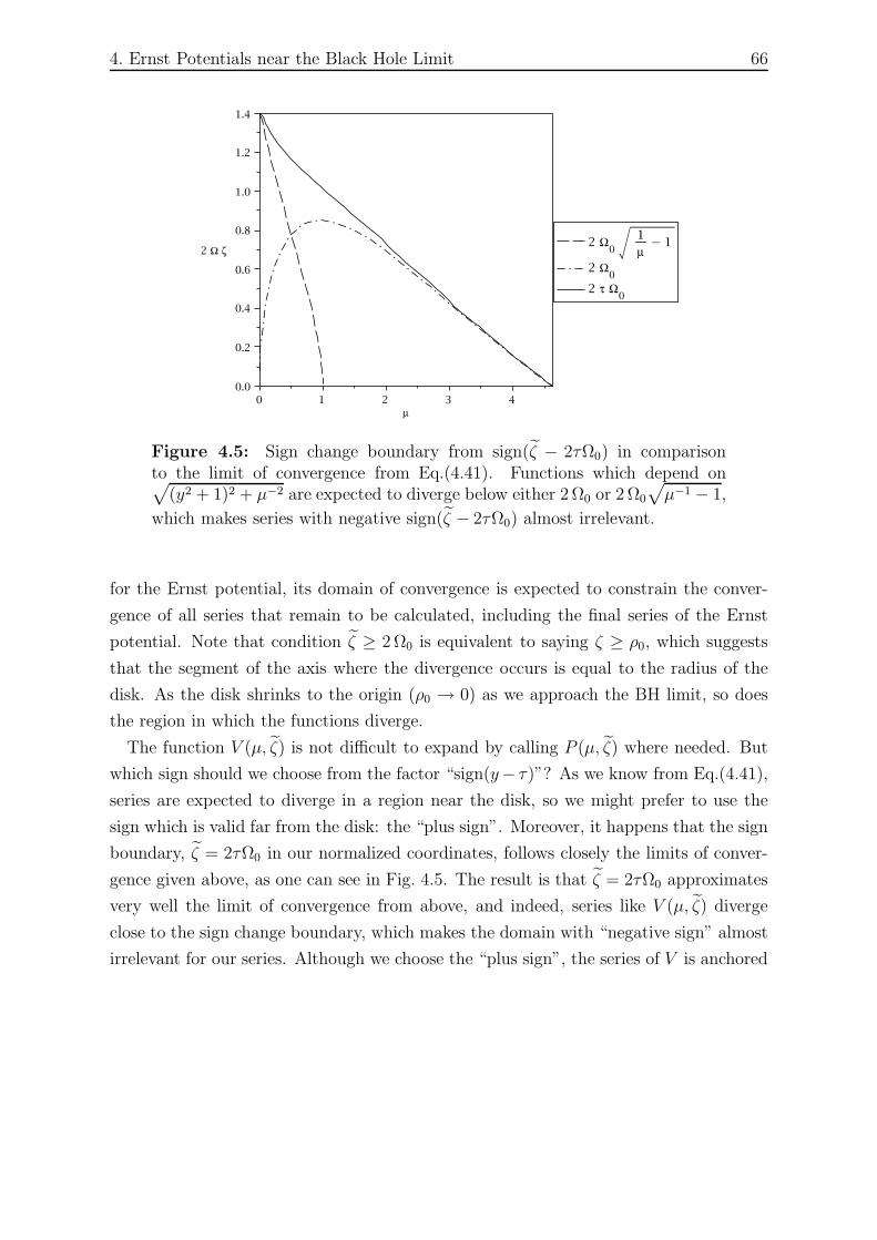
4. Ernst Potentials near the Black Hole Limit 66
2 W0
1mK 1
2 W0
2 t W0
m0 1 2 3 4
2 W z
0.0
0.2
0.4
0.6
0.8
1.0
1.2
1.4
Figure 4.5: Sign change boundary from sign(ζ − 2τΩ0) in comparisonto the limit of convergence from Eq.(4.41). Functions which depend on√
(y2 + 1)2 + µ−2 are expected to diverge below either 2 Ω0 or 2 Ω0
√µ−1 − 1,
which makes series with negative sign(ζ − 2τΩ0) almost irrelevant.
for the Ernst potential, its domain of convergence is expected to constrain the conver-
gence of all series that remain to be calculated, including the final series of the Ernst
potential. Note that condition ζ ≥ 2 Ω0 is equivalent to saying ζ ≥ ρ0, which suggests
that the segment of the axis where the divergence occurs is equal to the radius of the
disk. As the disk shrinks to the origin (ρ0 → 0) as we approach the BH limit, so does
the region in which the functions diverge.
The function V (µ, ζ) is not difficult to expand by calling P (µ, ζ) where needed. But
which sign should we choose from the factor “sign(y− τ)”? As we know from Eq.(4.41),
series are expected to diverge in a region near the disk, so we might prefer to use the
sign which is valid far from the disk: the “plus sign”. Moreover, it happens that the sign
boundary, ζ = 2τΩ0 in our normalized coordinates, follows closely the limits of conver-
gence given above, as one can see in Fig. 4.5. The result is that ζ = 2τΩ0 approximates
very well the limit of convergence from above, and indeed, series like V (µ, ζ) diverge
close to the sign change boundary, which makes the domain with “negative sign” almost
irrelevant for our series. Although we choose the “plus sign”, the series of V is anchored

4. Ernst Potentials near the Black Hole Limit 67
(µ = µ0) on a negative value:
V (µ, ζ) = − 0.055908 +
(0.012264 +
0.0013618
ζ
)(µ − µ0)
+
(−0.0026412 − 6.6713 × 10⁻⁴
ζ+
0.0064947
ζ2
)(µ − µ0)
2
+
(5.5869 × 10⁻⁴ − 2.1410 × 10⁻⁴
ζ− 0.0023506
ζ2− 2.3723 × 10⁻⁴
ζ3
)(µ − µ0)
3
+ O[(µ − µ0)4] . (4.42)
The remaining functions Z(µ, ζ), U(µ, ζ) and T (µ, ζ) depend all on the elliptic inte-
grals given by X(µ, ζ) and Y (µ, ζ). Since we restrict ourselves from now on to the “plus
sign” domain, the latter functions become simply X = E(υ, h′) and Y = F (υ, h′). The
derivatives needed for the series are all defined in Appendix A, but one must be careful
to compute a routine which generates series out of elliptic functions in a reasonable
amount of computation time and memory. Instead of using recursivly Eqs(A.7) for each
derivative of the Jacobian elliptic functions, a better strategy is to produce instead series
of these functions by expanding the right hand sides of
υ = am(Y, h′) = arcsin
[√1 − hP
h′
],
sin(υ) = sn(Y, h′) =
√1 − hP
h′,
cos(υ) = cn(Y, h′) =
√h (P − h)
h′,
√1 − h′2 sin2(υ) = dn(Y, h′) =
√hP .
Then, the Taylor series of F (υ, h′) and E(υ, h′) can be computed as series containing
derivatives of the Jacobian elliptic functions. Each time that the derivatives of Jacobian
elliptic functions need to be evaluated, the answer can be easily picked up in the four
series obtained from above. By properly combining the series of F (υ, h′), E(υ, h′), K(h),
K(h′) and E(h′), we obtain:
Z(µ, ζ) = 0.0028257 +
(−0.0011830 +
1.9350 × 10⁻⁶
ζ
)(µ − µ0)
+
(3.6763 × 10⁻⁴ − 1.7627 × 10⁻⁶
ζ− 3.3002 × 10⁻⁴
ζ2
)(µ − µ0)
2
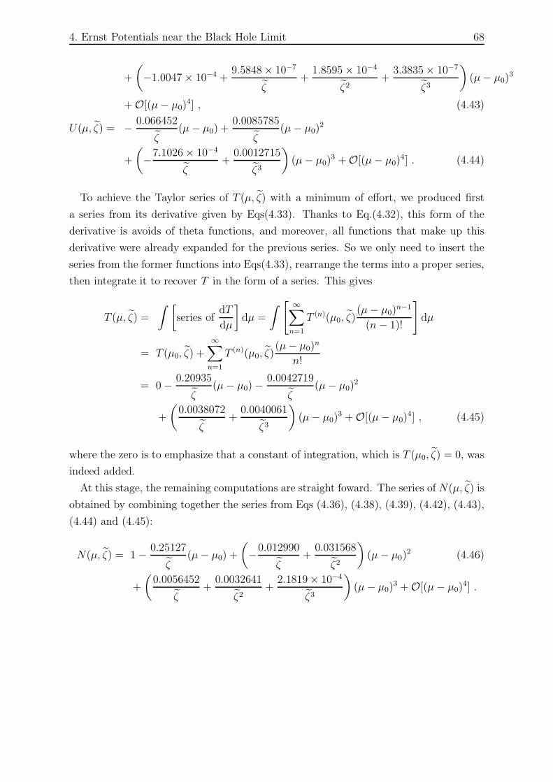
4. Ernst Potentials near the Black Hole Limit 68
+
(−1.0047 × 10⁻⁴ +
9.5848 × 10⁻⁷
ζ+
1.8595 × 10⁻⁴
ζ2+
3.3835 × 10⁻⁷
ζ3
)(µ − µ0)
3
+ O[(µ − µ0)4] , (4.43)
U(µ, ζ) = − 0.066452
ζ(µ − µ0) +
0.0085785
ζ(µ − µ0)
2
+
(−7.1026 × 10⁻⁴
ζ+
0.0012715
ζ3
)(µ − µ0)
3 + O[(µ − µ0)4] . (4.44)
To achieve the Taylor series of T (µ, ζ) with a minimum of effort, we produced first
a series from its derivative given by Eqs(4.33). Thanks to Eq.(4.32), this form of the
derivative is avoids of theta functions, and moreover, all functions that make up this
derivative were already expanded for the previous series. So we only need to insert the
series from the former functions into Eqs(4.33), rearrange the terms into a proper series,
then integrate it to recover T in the form of a series. This gives
T (µ, ζ) =
∫ [series of
dT
dµ
]dµ =
∫ [ ∞∑
n=1
T (n)(µ0, ζ)(µ − µ0)
n−1
(n − 1)!
]dµ
= T (µ0, ζ) +
∞∑
n=1
T (n)(µ0, ζ)(µ − µ0)
n
n!
= 0 − 0.20935
ζ(µ − µ0) −
0.0042719
ζ(µ − µ0)
2
+
(0.0038072
ζ+
0.0040061
ζ3
)(µ − µ0)
3 + O[(µ − µ0)4] , (4.45)
where the zero is to emphasize that a constant of integration, which is T (µ0, ζ) = 0, was
indeed added.
At this stage, the remaining computations are straight foward. The series of N(µ, ζ) is
obtained by combining together the series from Eqs (4.36), (4.38), (4.39), (4.42), (4.43),
(4.44) and (4.45):
N(µ, ζ) = 1 − 0.25127
ζ(µ − µ0) +
(−0.012990
ζ+
0.031568
ζ2
)(µ − µ0)
2 (4.46)
+
(0.0056452
ζ+
0.0032641
ζ2+
2.1819 × 10⁻⁴
ζ3
)(µ − µ0)
3 + O[(µ − µ0)4] .
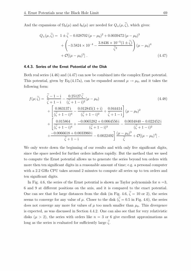
4. Ernst Potentials near the Black Hole Limit 69
And the expansions of Ω0(µ) and b0(µ) are needed for Q±(µ, ζ), which gives:
Q±(µ, ζ) = 1 ± ζ − 0.028702 (µ− µ0)2 + 0.0039472 (µ− µ0)
3
+
(−3.5824 × 10⁻⁴ − 3.8436 × 10⁻⁵(1 ± ζ)
ζ2
)(µ − µ0)
4
+ O[(µ − µ0)5] . (4.47)
4.4.3. Series of the Ernst Potential of the Disk
Both real series (4.46) and (4.47) can now be combined into the complex Ernst potential.
This potential, given by Eq.(4.17a), can be expanded around µ → µ0, and it takes the
following form:
f(µ; ζ) =ζ − 1 − i
ζ + 1 − i− 0.25127 ζ
(ζ + 1 − i)2(µ − µ0) (4.48)
+
[0.063137 i
(ζ + 1 − i)3− 0.012845(1 + i)
(ζ + 1 − i)2+
0.044414
ζ + 1 − i
](µ − µ0)
2
+
[0.015864
(ζ + 1 − i)4+
−0.0065282 + 0.0064556 i
(ζ + 1 − i)3− 0.0034840− 0.022452 i
(ζ + 1 − i)2
+−0.0066618 + 0.0033960 i
ζ + 1 − i− 0.0022492
](µ − µ0)
3
ζ+ O[(µ − µ0)
4] .
We only wrote down the beginning of our results and with only five significant digits,
since the space needed for further orders inflates rapidly. But the method that we used
to compute the Ernst potential allows us to generate the series beyond ten orders with
more then ten significant digits in a reasonable amount of time; e.g. a personal computer
with a 2.2 GHz CPU takes around 2 minutes to compute all series up to ten orders and
ten significant digits.
In Fig. 4.6, the series of the Ernst potential is shown as Taylor polynomials for n =3,
6 and 9 at different positions on the axis, and it is compared to the exact potential.
One can see that for large distances from the disk (in Fig. 4.6, ζ = 10 or 2), the series
seems to converge for any value of µ. Closer to the disk (ζ = 0.5 in Fig. 4.6), the series
does not converge any more for values of µ too much smaller than µ0. This divergence
is expected, as was discussed in Section 4.4.2. One can also see that for very relativistic
disks (µ > 2), the series with orders like n = 3 or 6 give excellent approximations as
long as the series is evaluated for sufficiently large ζ.
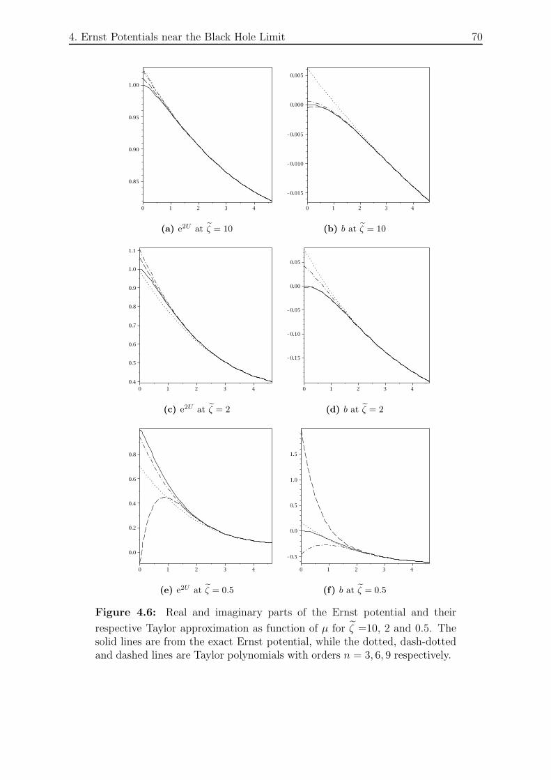
4. Ernst Potentials near the Black Hole Limit 70
0 1 2 3 4
0.85
0.90
0.95
1.00
(a) e2U at ζ = 10
0 1 2 3 4
K0.015
K0.010
K0.005
0.000
0.005
(b) b at ζ = 10
0 1 2 3 40.4
0.5
0.6
0.7
0.8
0.9
1.0
1.1
(c) e2U at ζ = 2
0 1 2 3 4
K0.15
K0.10
K0.05
0.00
0.05
(d) b at ζ = 2
0 1 2 3 4
0.0
0.2
0.4
0.6
0.8
(e) e2U at ζ = 0.5
0 1 2 3 4
K0.5
0.0
0.5
1.0
1.5
(f) b at ζ = 0.5
Figure 4.6: Real and imaginary parts of the Ernst potential and their
respective Taylor approximation as function of µ for ζ =10, 2 and 0.5. Thesolid lines are from the exact Ernst potential, while the dotted, dash-dottedand dashed lines are Taylor polynomials with orders n = 3, 6, 9 respectively.
4. Ernst Potentials near the Black Hole Limit 71
Analogous Taylor series can be computed using the other normalized and dimension-
less coordinate, ζ ≡ ζ/M , which we already introduced earlier in this work. The method
to find these series is the same as before, so we do not need to present each step again.
The final result starts with:
f(µ; ζ) =ζ − 1 − i
ζ + 1 − i− 0.025836 i
(ζ + 1 − i)2(µ − µ0)
2 (4.49)
+−0.0062737 + 0.0032261 i ζ
ζ (ζ + 1 − i)2(µ − µ0)
3 + O[(µ − µ0)4] .
The latter normalization (ζ) shows again series that are systematically more concise
than the former normalization; this was also true for the black hole series in section 4.2.
We can already see that the beginning of Eq.(4.49) agrees with what we conjectured in
Eq.(4.9) since the first order correction vanishes, although the two series do not use the
same expansion term for the next orders (ε vs (µ − µ0)). Similarly, the two first terms
of Eq.(4.48) should agree with what we conjectured in Eq.(4.8). This can be seen if ε
from this second series is expanded in a power series of the disk parameter (µ − µ0):
ε = 1 − M(µ) = −dM
dµ(µ0)(µ − µ0) + O[(µ − µ0)
2].
By picking the numerical value from Eq.(4.26), we find then that both series agree since
the second term of the black hole becomes:
2ζ
(ζ + 1 − i)2ε = − 2ζ
(ζ + 1 − i)2
dM
dµ(µ0)(µ − µ0) + O[(µ − µ0)
2]
= −0.2512727428 ζ
(ζ + 1 − i)2(µ − µ0) + O[(µ − µ0)
2] .
It means that the coefficient 0.25127... does not represent a quantity which distinguishes
the disk from a black hole with the same mass M and angular velocity Ω: it is a mere
effect of the choice of the expansion parameter (within the class of uniformly rotating,
stationary and axisymmetric bodies).
On the other hand, the coefficients of further expansion terms vary depending on what
kind of body the source is. In this manner, they allow us to identify whether we have
a black hole or some uniformly rotating fluid. Comparing Eqs(4.14) and (4.49), we find
that both the black hole and the disk of dust have potentials with the following structure
4. Ernst Potentials near the Black Hole Limit 72
on the axis:
f(ε; ζ) =ζ − 1 − i
ζ + 1 − i+
C2 i
(ζ + 1 − i)2ε2 + O(ε3) (4.50)
where C2 is a coefficient which is different for both bodies. If we take the series for 2ΩM
in Table 4.1, we find:
ε = 1 − 2ΩM = −1.2563637 × 10⁻¹(µ − µ0) + O[(µ − µ0)2] ,
(µ − µ0)2 = 63.353298 ε2 + O(ε3) .
The last result can be used to substitute (µ−µ0)2 by ε2 in Eq.(4.49), which thus provides
the series with the same relativistic parameter ε used for the black hole. We finally find
out that the characteristic coefficient C2 is, for the two bodies:
C2 = +1 for the Kerr black hole,
C2 = −1.636816606... for the disk of dust.
It would be interesting to know if other bodies such as rings have also the same form as
given in Eq.(4.50).
In Fig. 4.7, we compare Eq.(4.50) up to ε2 with the respective exact functions for the
disk and the black hole, using the coordinate ζ. The different behaviours can be seen
near the source (ζ < 3) for the Ernst potentials and their approximations; in the far
field, the correction terms wane and the Ernst potentials are essentially identical to a
extreme Kerr BH of the same mass (see Eq.(4.11)). For the black hole, the series up to
ε2 follows the exact potential closely. The approximation for e2U even crosses zero into
negative values near the centre, suggesting that the source might have a horizon7. For
the disk, both curves of e2U stay positive everywhere.
If we compare the series of the Ernst potential at the centre of the disk8, f0 = e2V0 +ib0,
with our two series (4.48) and (4.49) at the origin of the normalized axis, ζ = ζ = 0, the
result might look surprising as they are not the same:
f0(µ) = −i + (0.0061997 + 0.028702 i) (µ − µ0)2 + O[(µ − µ0)
3] ,
f(µ; ζ = 0) = −i + 0.012918 (µ− µ0)2 +
(higher orders diverge to ∞ as ζ → 0
),
f(µ; ζ = 0) = −i + 0.012918 (µ− µ0)2 +
(higher orders diverge to ∞ as ζ → 0
).
7on the axis, the horizon is situated where e2U = 0.8The Ernst potential is identical on the axis ζ with either non-rotating or co-rotating coordinate.
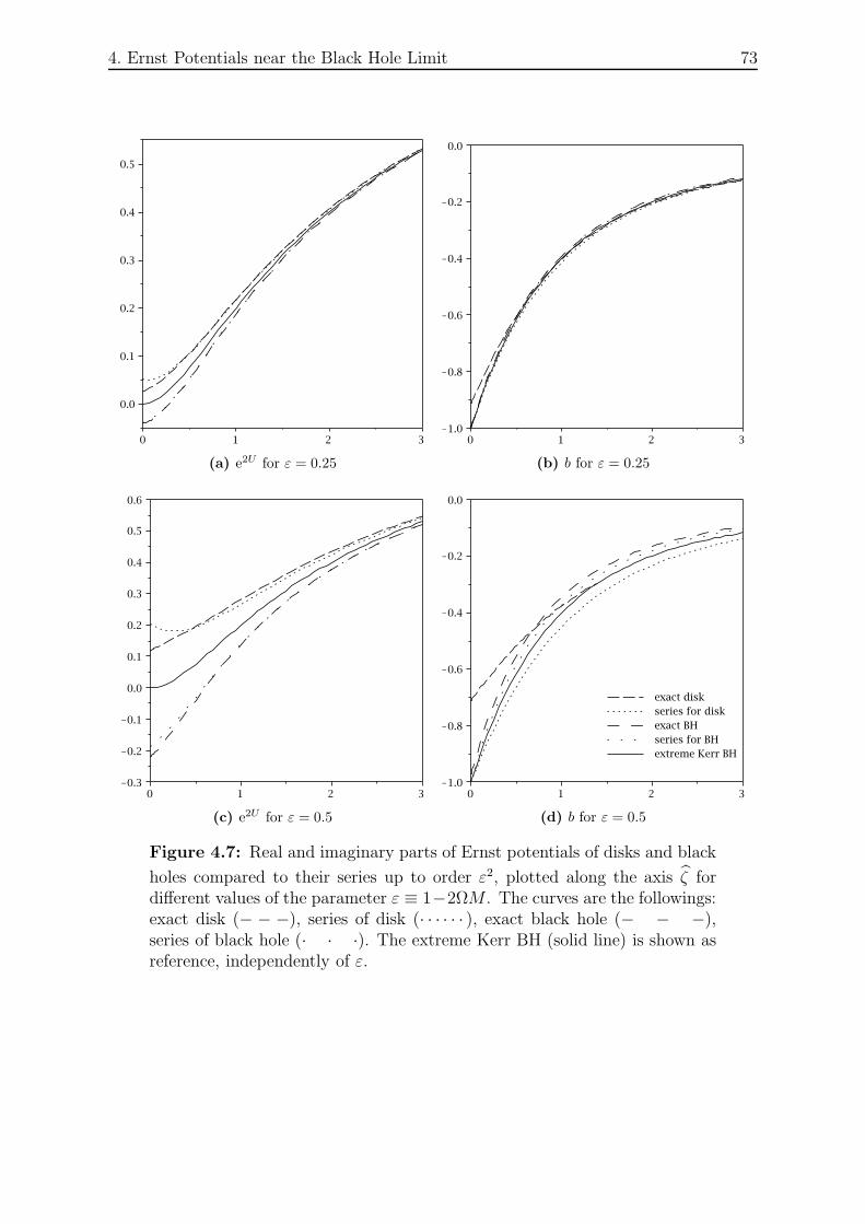
4. Ernst Potentials near the Black Hole Limit 73
0 1 2 3
0.0
0.1
0.2
0.3
0.4
0.5
(a) e2U for ε = 0.25
0 1 2 3K1.0
K0.8
K0.6
K0.4
K0.2
0.0
(b) b for ε = 0.25
0 1 2 3K0.3
K0.2
K0.1
0.0
0.1
0.2
0.3
0.4
0.5
0.6
(c) e2U for ε = 0.5
series for diskexact BHseries for BHextreme Kerr BH
exact disk
0 1 2 3K1.0
K0.8
K0.6
K0.4
K0.2
0.0
(d) b for ε = 0.5
Figure 4.7: Real and imaginary parts of Ernst potentials of disks and black
holes compared to their series up to order ε2, plotted along the axis ζ fordifferent values of the parameter ε ≡ 1−2ΩM . The curves are the followings:exact disk (− − −), series of disk (· · · · · · ), exact black hole (− − −),series of black hole (· · ·). The extreme Kerr BH (solid line) is shown asreference, independently of ε.
4. Ernst Potentials near the Black Hole Limit 74
This difference can be explained by the normalization of the coordinate system and the
unique property of the extreme Kerr BH geometry. As explained in section 2.3.2, the
disk of dust, in its extreme Kerr BH limit, is contained in an “inner world” which is
separated from an “outer world” by an infinitely long “throat geometry”. The normalized
coordinate that we chose for the series, ζ ≡ 2Ωζ and ζ ≡ ζ/M , are such that the disk
shrinks to the origin as we approach the BH limit: it describes then an asymptotically
flat spacetime with a degenerate black hole horizon at the origin. If we had chosen a
different normalization such as y = ζ/ρ0, the coordinate system would have ended up
describing the inner world: a disk of dust with finite radius surrounded by the throat
geometry in the far field.
5. Conclusion
We began our work by investigating in chapter 3 the relativistic solutions of fluid bodies
made of strange quark matter. Through sequences of highly accurate numerical solu-
tions, it was possible to identify extremal solutions (maximal mass, angular momentum,
etc.) and to define the limits of these fluids in equilibrium with great precision.
Whereas it is known analytically that the EOS describing strange matter tends to
that of a homogeneous body in the Newtonian limit, we saw here that sequences of
configurations with these two EOS are similarly bounded by a mass-shedding limit,
an infinite central pressure, the extreme Kerr black hole limit, etc. All continuously
connected solutions are said to form a “class”. Strange matter bodies can be divided
up into the same classes as for homogeneous fluids: a “Schwarzschild class” containing
only spheroids, and a “ring class” where continuous transitions between spheroidal and
toroidal bodies exist, etc. But strange stars also have characteristics which distinguish
them from homogeneous bodies. We have shown in Figs 3.2, 3.3 and 3.4, that a domain
of the Schwarzschild class is unstable. Indeed, along sequences of constant angular
momentum, maximal masses are found at intermediate configurations. The accuracy of
our solutions allowed us to find that the configurations in the class with maximal mass
or maximal angular momentum are not exactly at the mass-shedding limit, contrary to
what was believed.
It was also shown numerically that a parametric transition exists from strange matter
rings to the extreme Kerr BH. It is expected that E ≤ 1 always holds on the surface
of a fluid body. Indeed, this inequality was used to prove that for rotating fluids the
extreme Kerr black hole necessarily results if e2V0 → 0 [Mei06]. We have verified that
this inequality is correct for a large class of rings. Figs 3.7 and 3.8 suggest that the
transition to the black hole is rather slow as e2V0 → 0. This can be made more precise
through the comparison with the Kerr solution, which leads us to conjecture that for
every stationary rotating body permitting a transition to a black hole, the multipole
moments yn tend to one according to the formula
dyn
dy0(y0 = 1) = n + 1 . (5.1)
75
5. Conclusion 76
The plots of the multipole moments provide evidence suggesting that any given moment
yn, n > 0, of such bodies is always greater than that of the Kerr solution with the
same y0. It then follows that the Kerr metric could never represent the exterior of these
configurations.
In chapter 4, we discussed again the multipoles and the result from Eq.(5.1) by using
two types of normalization. There it was found that the conjecture for n = 1 in Eq.(5.1)
is a consequence of the first “law of thermodynamics” for uniformly rotating fluids. If
the Ernst potential of a uniformly rotating fluid can be expanded by the relativistic
parameter 2ΩM near the extreme Kerr BH limit, we showed that Taylor series on the
positive part of the axis would read
f =ζ/M − 1 − i
ζ/M + 1 − i+ ∅ + O[(1 − 2ΩM)2] ,
where the first term is from the extreme Kerr BH solution and the vanishing first cor-
rection term is equivalent to the previous conjecture. Using the Ernst potential on the
axis of the uniformly rotating disk of dust, we first proved that the conjecture indeed
holds for this body by computing the derivative of the potential. Then, we developed
a computer routine which can generate the Taylor series of the Ernst potential for the
disk up to arbitrary order. Although it might only be useful for few expansion terms
near the black hole limit, the series indeed seems to converge for the entire sequence of
disk configurations and everywhere on the axis, except for a tiny segment near the disk.
As our knowledge of astrophysical collapse scenarios improves, it will be interesting to
see how strong the connections can be to the quasi-stationary collapse considered here.
Although the conjecture from Eq.(5.1) holds for the disk and our sequences of rings,
it is proved for uniformly rotating fluids only for n = 1. It would also be interesting
to provide an explanation of this conjecture for the further multipoles. And again, as
the series for the black hole and the disk both begin with the same structure given in
Eq.(4.50), one can ask if this form also holds for other bodies near the extreme Kerr BH
limit, such as rings.
Bibliography
[AFK+04] M. Ansorg, T. Fischer, A. Kleinwachter, R. Meinel, D. Petroff, and
K. Schobel. Equilibrium configurations of homogeneous fluids in general
relativity. Mon. Not. R. Astron. Soc., 355:682, 2004.
[AFO86] C. Alcock, E. Farhi, and A. Olinto. Strange stars. Astrophys. J., 310:261–
272, 1986.
[AK04] A. Ashtekar and B. Krishnan. Isolated and dynamical horizons and their
applications, 2004. Online Publication: Referenced on December 12, 2005,
http://www.livingreviews.org/lrr-2004-10.
[AKM03a] M. Ansorg, A. Kleinwachter, and R. Meinel. Highly accurate calculation
of rotating neutron stars: Detailed description of the numerical methods.
Astron. Astrophys., 405:711, 2003.
[AKM03b] M. Ansorg, A. Kleinwachter, and R. Meinel. Relativistic Dyson rings and
their black hole limit. Astrophys. J. Lett., 582:L87, 2003.
[BH99] J. Bardeen and G. T. Horowitz. Extreme Kerr throat geometry: A vacuum
analog of AdS2 × S2. Phys. Rev. D, 60:104030, 1999.
[BHM+05] L. Baiotti, I. Hawke, P. J. Montero, F. Loffler, L. Rezzolla, N. Stergioulas,
J. A. Font, and E. Seidel. Three-dimensional relativistic simulations of
rotating neutron-star collapse to a Kerr black hole. Phys. Rev. D, 71:024035,
2005.
[BL67] R. H. Boyer and R. W. Lindquist. Maximal analytic extension of the kerr
metric. J. Math. Phys., 8:265, 1967.
[BPT72] J. M. Bardeen, W. H. Press, and S. A. Teukolsky. Rotating black holes:
Locally nonrotating frames, energy extraction, and scalar synchrotron ra-
diation. Astrophys. J., 178:347, 1972.
77
Bibliography 78
[Buc59] H. A. Buchdahl. General relativistic fluid spheres. Phys. Rev., 116(4):1027–
1034, Nov 1959.
[BW69] J. M. Bardeen and R. V. Wagoner. Uniformly rotating disks in general
relativity. Astrophys. J., 158:L65, 1969.
[BW71] J. M. Bardeen and R. V. Wagoner. Relativstic disks. I. uniform rotation.
Astrophys. J., 167:359, 1971.
[Cha31] S. Chandrasekhar. The Maximum Mass of Ideal White Dwarfs. Astrophys.
J., 74:81–82, July 1931.
[CJJ+74] A. Chodos, R. L. Jaffe, K. Johnson, C. B. Thorn, and V. F. Weisskopf.
New extended model of hadrons. Phys. Rev. D, 9(12):3471–3495, Jun 1974.
[CJJT74] A. Chodos, R. L. Jaffe, K. Johnson, and C. B. Thorn. Baryon structure in
the bag theory. Phys. Rev. D, 10(8):2599–2604, Oct 1974.
[Ern68] F. J. Ernst. New formulation of the axially symmetric gravitational field
problem. Phys. Rev., 167:1175, 1968.
[FHA05] T. Fischer, S. Horatschek, and M. Ansorg. Uniformly rotating rings in
general relativity. Mon. Not. R. Astron. Soc., 364:943, 2005.
[FHP89] G. Fodor, C. Hoenselaers, and Z. Perjes. Multipole moments of axisym-
metric systems in relativity. J. Math. Phys., 30(10):2252, 1989.
[FJ84] E. Farhi and R. L. Jaffe. Strange matter. Phys. Rev. D, 30(11):2379–2390,
Dec 1984.
[FK09] R. Filter and A Kleinwachter. On the multipole moments of a rigidly
rotating fluid body. Ann. Phys. (Berlin), 18:102, 2009.
[Fon03] J. A. Font. Numerical hydrodynamics in general relativity,
2003. Online Publication: Referenced on December 12, 2005,
http://www.livingreviews.org/lrr-2003-4.
[Ger70] R. Geroch. Multipole moments. II. curved space. J. Math. Phys.,
11(8):2580, 1970.
[GHL+99] E. Gourgoulhon, P. Haensel, R. Livine, E. Paluch, S. Bonazzola, and J. A.
Marck. Fast rotation of strange stars. Astron. Astrophys., 349:851, 1999.
Bibliography 79
[GR94] I. S. Gradshteyn and I. M. Ryzhik. Table of Integrals, Series and Products.
Academic Press Inc, 5th revised edition, 1994.
[Han73] R. O. Hansen. Multipole moments of stationary space-times. J. Math.
Phys., 15(1):46, 1973.
[HS67] J. B. Hartle and D. H. Sharp. Variational principle for the equilibrium of
a relativistic, rotating star. Astrophys. J., 147:317, 1967.
[Ker63] R. P. Kerr. Gravitational field of a spinning mass as an example of alge-
braically special metrics. Phys. Rev. Lett., 11:237, 1963.
[KLM10] A. Kleinwachter, H. Labranche, and R. Meinel. On the black hole limit of
rotating disks and rings. (in preparation), 2010.
[KMN95] A. Kleinwachter, R. Meinel, and G. Neugebauer. The multipole moments of
the rigidly rotating disk of dust in general rleativity. Phys. Lett. A, 200:82,
1995.
[KN68] D. Kramer and G. Neugebauer. Zu axialsymmetrischen stationaren
Losungen der Einsteinschen Feldgleichungen fur das Vakuum. Commu-
nications in Mathematical Physics, 10:132–139, June 1968.
[Kor95] P. Kordas. Reflection-symmetric, asymptotically flat solutions of the vac-
uum axistationary Einstein equations. Class. Quantum Grav., 12:2037,
1995.
[KT66] W. Kundt and M. Trumper. Orthogonal decomposition of axi-symmetric
stationary spacetimes. Zeitschrift fur Physik, 192:419–422, August 1966.
[KWWG95] Ch. Kettner, F. Weber, M. K. Weigel, and N. K. Glendenning. Structure
and stability of strange and charm stars at finite temperatures. Phys. Rev.
D, 51(4):1440–1457, Feb 1995.
[Lin92] L. Lindblom. On the symmetries of equilibrium stellar models. Philos.
Trans. R. Soc. London, Ser. A, 340:353, 1992.
[LPA07] H. Labranche, D. Petroff, and M. Ansorg. The parametric transition of
strange matter rings to a black hole. Gen. Rel. and Grav., 39:129–143,
2007.
Bibliography 80
[MAK+08] R. Meinel, M. Ansorg, A. Kleinwachter, G. Neugebauer, and D. Petroff. Rel-
ativistic Figures of Equilibrium. Cambridge University Press, Cambridge,
2008.
[Mei02] R. Meinel. Black holes: A physical route to the Kerr metric. Ann. Phys.
(Leipzig), 11:509–521, August 2002.
[Mei04] R. Meinel. Quasistationary collapse to the extreme Kerr black hole. Ann.
Phys. (Leipzig), 13:600–603, October 2004.
[Mei06] R. Meinel. On the black hole limit of rotating fluid bodies in equilibrium.
Class. Quantum Grav., 23:1359, 2006.
[MK95] R. Meinel and A. Kleinwachter. Dragging effects near a rigidly rotating disk
of dust. In J. B. Barbour and H. Pfister, editors, Mach’s Principle: From
Newton’s Bucket to Quantum Gravity, page 339, Boston, 1995. Birkhauser.
[MN95] R. Meinel and G. Neugebauer. Asymptotically flat solutions to the Ernst
equation with reflectional symmetry. Class. Quantum Grav., 12:2045, 1995.
[NM93] G. Neugebauer and R. Meinel. The Einsteinian gravitational field of a
rigidly rotating disk of dust. Astrophys. J., 414:L97, 1993.
[NM94] G. Neugebauer and R. Meinel. General relativistic gravitational field of a
rigidly rotating disk of dust: Axis potential, disk metric, and surface mass
density. Phys. Rev. Lett., 73:2166, 1994.
[NM95] G. Neugebauer and R. Meinel. General relativistic gravitational field of a
rigidly rotating disk of dust: Solution in terms of ultraelliptic functions.
Phys. Rev. Lett., 75:3046–3047, October 1995.
[SA03] K. Schobel and M. Ansorg. Maximal mass of uniformly rotating homoge-
neous stars in einsteinian gravity. Astron. Astrophys., 405:405, 2003.
[Web05] F. Weber. Strange quark matter and compact stars. Prog. Part. Nucl.
Phys., 54:193–288, 2005.
A. Elliptic Integrals and Functions
This appendix provides our definitions of the different functions related to elliptic inte-
grals and some useful relations or identities. Most definitions, conventions or notations
are inspired from [GR94].
Elliptic integral of the first and second kind respectively:
F (φ, k) :=
φ∫
0
dθ√1 − k2 sin2 θ
=
sin φ∫
0
dx√(1 − x2)(1 − k2x2)
(A.1)
E(φ, k) :=
φ∫
0
√1 − k2 sin2 θdθ =
sinφ∫
0
√1 − k2x2
1 − x2dx (A.2)
The number k is called the modulus of these integrals, and k′ :=√
1 − k2 is called the
complementary modulus.
Complete elliptic integrals:
K(k) := F(π2, k)
, E(k) := E(π2, k)
. (A.3)
Functional relations between elliptic integrals:
E(k)K(k′) + K(k)E(k′) − K(k)K(k′) =π
2(A.4)
∂F (φ, k)
∂φ=
1√1 − k2 sin2 φ
, (A.5a)
∂F (φ, k)
∂k=
1
k′2
(E(φ, k) − k′2F (φ, k)
k− k sin φ cosφ√
1 − k2 sin2 φ
), (A.5b)
∂E(φ, k)
∂φ=
√1 − k2 sin2 φ , (A.5c)
∂E(φ, k)
∂k=
E(φ, k) − F (φ, k)
k. (A.5d)
81
A. Elliptic Integrals and Functions 82
Jacobian elliptic functions:
u := F (φ, k)
am u ≡ am(u, k) := φ , (A.6a)
sn u ≡ sn(u, k) := sin φ , (A.6b)
cn u ≡ cn(u, k) := cos φ , (A.6c)
dn u ≡ dn(u, k) :=
√1 − k2 sin2 φ . (A.6d)
Derivatives of the Jacobian elliptic functions:
∂am u
∂u= dn u , (A.7a)
∂sn u
∂u= cn u dn u , (A.7b)
∂cn u
∂u= − sn u dn u , (A.7c)
∂dn u
∂u= − k2sn u cn u , (A.7d)
∂am u
∂k=
dn u
kk′2
[−E(am u, k) + k′2u + k2 sn u cn u
dn u
], (A.7e)
∂sn u
∂k=
dn u cn u
kk′2
[−E(am u, k) + k′2u + k2 sn u cn u
dn u
], (A.7f)
∂cn u
∂k= − dn u sn u
kk′2
[−E(am u, k) + k′2u + k2 sn u cn u
dn u
], (A.7g)
∂dn u
∂k= − k sn u cn u
k′2
[−E(am u, k) + k′2u +
sn u dn u
cn u
]. (A.7h)
Heuman’s Lambda function:
Λ0(φ, k) :=2
π[E(k)F (φ, k′) + K(k)E(φ, k′) − K(k)F (φ, k′)] (A.8)
Jacobian Zeta function:
Z(u, k) := E(am u, k) − E(k)
K(k)u (A.9)
A. Elliptic Integrals and Functions 83
Jacobian theta functions:
ϑ1(w, B) =∞∑
n=−∞
(−1)n exp[
12(2n + 1)
]2B + (2n + 1)w
, (A.10a)
ϑ2(w, B) =∞∑
n=−∞
exp[
12(2n + 1)
]2B + (2n + 1)w
, (A.10b)
ϑ3(w, B) =
∞∑
n=−∞
expn2B + 2nw
, (A.10c)
ϑ4(w, B) =
∞∑
n=−∞
(−1)n expn2B + 2nw
. (A.10d)
One particular partial derivative with ϑ2:
∂
∂wln(ϑ2(w, B)
)= Λ0
(am(u, k′) , k
)(A.11)
with w =πu
2K(k)and B = −π
K(k′)
K(k)
One general property with partial derivatives of ϑ2:
∂
∂Bϑ2(w, B) =
1
4
∂2
∂w2ϑ2(w, B) (A.12)
B. Some Useful Functions for the Disk of Dust
B.1. List of Functions in the Ernst Potential of the Disk
Functions which depend only on the relativistic parameter µ:
τ = 4
√1 +
1
µ2,
h =
√1
2
(1 +
1√µ−2 + 1
),
h′ =
√1
2
(1 − 1√
µ−2 + 1
),
g(x) =ln(
√1 + x2 + x)√1 + x2
=arcsinh x√
1 + x2
(=
1
2
d
dx[arcsinh x]2
),
In =1
π
µ∫
0
g(x) xn
√µ − x
dx ,
I = 4
√1 + µ2 I0 =
4
√1 + µ2
π
µ∫
0
ln(√
1 + x2 + x)√1 + x2
√µ − x
dx ,
am ≡ am(I, h′), sn ≡ sn(I, h′), cn ≡ cn(I, h′), dn ≡ dn(I, h′) ,
c1 =1õ
2 4
√1 + µ2 E(am , h′) − (µ +
√1 + µ2)I0 + I1
,
e2V0 =h′cn 2
h, b0 = −sn dn
h,
Ω0 ≡ Ωρ0 =1
2
√1 − h′2
h2cn ,
M ≡ 2ΩM = −b0 − Ω0c1 ,
The functions “am”, “sn”, “cn” and “dn” call the Jacobian elliptic functions which are
defined in Appendix A.
84
B. Some Useful Functions for the Disk of Dust 85
Functions which depend only on µ and the axis coordinate ζ :
y =ζ
ρ0=
ζ
2Ω0=
M
2Ω0ζ ,
R =y√
µ
π√
(y2 + 1)2 + µ−2
µ∫
0
x(y2 + 1) + µ−1
µ(y2 + 1) − x· g(x)√
µ − xdx ,
S =h′(y2 − τ 2)
2√
(y2 + 1)2 + µ−2,
P =
√(y2 + 1)2 + µ−2 + 2hτy
(y + τ)2,
V = sign(y − τ)h√
P (1 − hP )(P − h)
1 − hP − h′,
υ = arcsin
[√1 − hP
h′
],
X = sign(y − τ)E(υ, h′) ,
Y = sign(y − τ)F (υ, h′) ,
Z = X − E(h′)
K(h′)Y ,
U =π
4K(h)
(2Y
K(h′)− 1
),
W± =π
2K(h)
[I ±
(Y − K(h′)
2
)],
T = ln ϑ2
(W+ ,−π
K(h′)
K(h)
)− ln ϑ2
(W− ,−π
K(h′)
K(h)
),
N = exp
R − 2I (S + V + Z + U) + T
,
Q± =1 − 2Ω2
0(y2 + 1 +
√(y2 + 1)2 + µ−2)
−b0 ∓ 2Ω0y.
Again, K, E, F and ϑ2 call elliptic functions which are defined in Appendix A. Finally,
the complex Ernst potential on the axis of the rigidly rotating disk reads:
f(µ; y) =1 − iNQ−
N + iQ+
.
B. Some Useful Functions for the Disk of Dust 86
B.2. Some Other Useful Relations
The following identities can be useful:
h2 + h′2 = 1 , 2h h′ =1√
1 + µ2(B.1)
(1 − h − h′)(h − h′ − 1) = 2h(1 − h) ,h − h′ − 1
1 − h − h′=
h
1 − h′(B.2)
Some derivatives can take a recursive form:
dτ
dµ=
− τ
2µ(1 + µ2), (B.3a)
dh
dµ= 2h2 h′3 , (B.3b)
dh′
dµ= − 2h′2 h3 , (B.3c)
dg(x)
dx=
1 − xg(x)
1 + x2. (B.3d)
Danksagung
Mein besonderer Dank gilt Prof. Reinhard Meinel fur die Moglichkeit der Promotion in
der Allgemeinen Relativitatstheorie am TPI in Jena und fur seine fachliche Betreuung
meiner Doktorarbeit. Besonders seine prazisen Erklarungen zu vielen meiner Fragen
uber die Gravitationstheorie waren sehr hilfreich.
Weiterhin danke ich Dr. David Petroff, Dr. Andreas Kleinwachter und Dr. Marcus Ansorg
fur die wissenschaftliche Unterstutzung, die massgeblich zum Gelingen meiner Arbeit
beitrug, Insbesondere danke ich Dr. David Petroff fur seine Hilfe bei bei der Berechnung
von Konfigurationen aus “strange quark matter” und fur das Korrekturlesen der Arbeit,
sowie Dr. Andreas Kleinwachter fur seine Unterstutzung bei der Untersuchung des Ernst-
Potentials der Staubscheibe, welche Voraussetzung fur die Berechnung der Taylor-Reihe
war.
Dank gilt auch meinen weiteren Kollegen Stefan Horatschek, Christian Teichmuller,
Michael Brugmann, Guillaume Faye sowie den Diplomanden des TPI fur die vielen
interessanten Diskussionen und die angenehme Arbeitsathmosphare.
Weiterhin danke ich meinen Eltern fur ihre liebevolle Ermunterung, sowie meinen Fre-
unden Marc Bergevin, Sylvie Brunet, David Cote und Vincent Bouchard, mit denen ich
meine Studienzeit in Montreal und mein Interesse an der Physik geteilt habe.
87

Ehrenwortliche Erklarung
Ich erklare hiermit ehrenwortlich, dass ich die vorliegende Arbeit selbststandig, ohne un-
zulassige Hilfe Dritter und ohne Benutzung anderer als der angegebenen Hilfsmittel und
Literatur angefertigt habe. Die aus anderen Quellen direkt oder indirekt ubernommenen
Daten und Konzepte sind unter Angabe der Quelle gekennzeichnet.
Niemand hat von mir unmittelbar oder mittelbar geldwerte Leistungen fur Arbeiten
erhalten, die im Zusammenhang mit dem Inhalt der vorgelegten Dissertation stehen.
Insbesondere habe ich hierfur nicht die entgeltliche Hilfe von Vermittlungs- bzw. Be-
ratungsdiensten (Promotionsberater oder andere Personen) in Anspruch genommen.
Die Arbeit wurde bisher weder im In- noch im Ausland in gleicher oder ahnlicher Form
einer anderen Prufungsbehorde vorgelegt.
Die geltende Promotionsordnung der Physikalisch-Astronomischen Fakultat ist mir
bekannt.
Ich versichere ehrenwortlich, dass ich nach bestem Wissen die reine Wahrheit gesagt und
nichts verschwiegen habe.
Jena, den 13. Januar 2010
Hendrick Labranche
88
Lebenslauf
Angaben zur Person
Name: Labranche, Hendrick
geboren am 2. Juli 1979 in Quebec, Quebec (QC), Kanada
Staatsangehorigkeit: kanadisch
Anschrift: Dornburger Str. 15, 07743 Jena
Schulausbildung
1985-1988 Ecole primaire Du Buisson, Sillery, QC
1988-1991 Ecole primaire Saint-Michel, Sillery, QC
1991-1996 Petit Seminaire de Quebec, QC
Abschluss: Diplome d’etudes secondaires
1996-1998 Petit Seminaire de Quebec, QC
Abschluss: Diplome d’etudes collegiales & International Baccalaureate Diploma
Ausbildung an der Universitat
1998-2001 Universite de Montreal, QC
Abschluss: B.Sc. en physique
2001-2003 University of Guelph, Ontario, Kanada
Abschluss: M.Sc. in Physics
2004-2010 Friedrich-Schiller-Universitat Jena
Abschluss: Dr. rer. nat. in Physik (eventuell
nach Abgabe der Dissertation in der ThULB)
89