parametric and semi-parametric approaches in the analysis of short-term effects of air pollution on...

Computational Statistics & Data Analysis 51 (2007) 4324–4336www.elsevier.com/locate/csda

Parametric and semi-parametric approaches in the analysis ofshort-term effects of air pollution on health

Michela Baccinia,b,∗, Annibale Biggeria,b, Corrado Lagazioc,Aitana Lertxundia,d, Marc Saezd

aDepartment of Statistics “G. Parenti”, University of Florence, Viale Morgagni, 59, 50134 Firenze, ItalybBiostatistics Unit, Institute for Cancer Prevention (CSPO), Florence, Italy

cDepartment of Statistical Sciences, University of Udine, ItalydResearch Group on Statistics, Applied Economics and Health (GRECS), University of Girona, Spain

Received 9 October 2004; received in revised form 23 September 2005; accepted 30 May 2006Available online 27 June 2006

Abstract

Generalized additive models (GAMs) have become the standard tool for the analysis of short-term effects of air pollution on humanhealth. Usually, the confounding effect of seasonality and long-term trend is described by flexible parametric or non-parametricfunctions of calendar time. Two different modeling strategies, i.e. GAM with penalized regression splines and GAM with regressionsplines, were compared by means of a simulation study, addressing attention to the inference on air pollutant effect. Simulationresults indicated that GAM with regression splines provides negligibly biased estimates of air pollutant effect and it is robust tomisspecification of the degrees of freedom of the spline. GAM with penalized regression splines requires a certain amount ofundersmoothing in order to reduce the bias of the estimates and to improve the coverage of confidence intervals. These findingsagree with asymptotic results developed in the context of partially splined models.© 2006 Elsevier B.V. All rights reserved.

Keywords: Generalized additive model; Smoothing spline; Regression spline; Penalized regression spline; Epidemiological time series; Airpollution

1. Introduction

Currently generalized additive models (GAMs) have become a standard in the analysis of short-term effects ofair pollution on health. In such models, non-parametric functions of time are used to control for those unobservedconfounders that could have a systematic but irregular temporal behavior (Schwartz, 1994). In many applicationsnon-parametric functions are also used to adjust for observed confounders such as weather variables (temperature andhumidity) (Samet et al., 2000; Katsouyanni et al., 2001) or influenza epidemics (Saez et al., 2002).

∗ Corresponding author. Department of Statistics “G. Parenti”, University of Florence, Viale Morgagni, 59, 50134 Firenze, Italy.Tel.: +39 055 4237475; fax: +39 055 4223560.

E-mail address: [email protected] (M. Baccini).

0167-9473/$ - see front matter © 2006 Elsevier B.V. All rights reserved.doi:10.1016/j.csda.2006.05.026

http://www.elsevier.com/locate/csda

mailto:[email protected]

M. Baccini et al. / Computational Statistics & Data Analysis 51 (2007) 4324–4336 4325

Recently, critical points concerning the use of commercial statistical software that implements backfitting algorithmto estimate GAMs were stressed (Knight, 2002; Kaiser, 2002). Specifically, they refer to the need of adopting morestringent convergence criteria in order to obtain unbiased estimates (Dominici et al., 2002) and, above all, they addressunderestimation of standard errors in presence of high concurvity, a non-parametric analogue of multicollinearity(Ramsay et al., 2003; Daniels et al., 2004). Re-analyses of time series data of air pollution and health were performed,in order to update previously published results (Dominici et al., 2002; The HEI Review Panel, 2003; Biggeri et al.,2002, 2005).

These problems have encouraged the use of alternative modeling strategies (Lumley and Sheppard, 2003). These arebased on simpler and more standard estimation methods, such as the approach based on the specification of GAM withregression splines (GAM + RS) (Dominici et al., 2002; Biggeri et al., 2002), standard error estimation based on lesscomputationally intensive procedures (Ramsay et al., 2003), or GAMs with penalized regression splines (GAM+PRS)

(Marx and Eilers, 1998; Ruppert et al., 2003; Wood, 2000). The new attention on GAMs has brought out aspects ofsemi-parametric modeling of epidemiological time series usually taken for granted, in particular the importance ofthe selection of the smoothing parameter and the consequences of this choice on the estimation of air pollutant effect(Dominici et al., 2004).

The purpose of our work is to compare the performances of GAM with regression splines and GAM with penalizedregression splines in estimating the parametric term which models the air pollutant effect in epidemiological timeseries regression. In this respect, the smooth function describing seasonality and trend of epidemiological time seriesis considered a (set of) nuisance parameter(s) and the interest is restricted to the specification of this term as long as itaffects the estimate of air pollutant effect.

To pursue our aim, first we compare the two approaches in a simulation study with varying effect size of air pollutant,amount of concurvity and seasonality in the outcome variable. Then we evaluate robustness of results to misspecificationof the degree of smoothing.

In Section 2 we describe the “standard” approach to the analysis of short-term effects of air pollution based onepidemiological time series and we discuss the alternative possibilities to adjust for time-related confounding usingspline-based terms. In Section 3 we report the main results concerning the asymptotic behavior of the parametric termestimator in a semi-parametric model. The model used to simulate pseudo-data and the simulation plan are describedin Section 4. The results are reported in Section 5 and discussed in Section 6.

2. The “standard” model

In its simplest form (with only one smooth term), the “standard” model used for epidemiological time series analysisis the following:

yt ∼ Poisson (�t ) ,

log (�t ) = �0 + f (t) +∑

i

�ixit , (1)

where yt is, for instance, the number of deaths or hospital admissions in the day t, f (t) is a generic smooth function oftime, xit is the value of the ith explanatory variable at time t and

(�0, �1, . . . , �I

)is a vector of unknown parameters. The

explanatory variables include air pollutant concentration and confounding variables (namely temperature, humidity,influenza epidemics, day of the week, holidays).

The model can eventually take into account for overdispersion; in this case a dispersion parameter is estimated andsuccessively used to inflate the standard errors of the Poisson model coefficients.

Different approaches can be used to specify the smooth term in (1). Locally weighted regression smoothers(Cleveland, 1979), or, more frequently, spline-based functions (regression splines, smoothing splines and penalizedregression splines) are used. In the next sections the three different spline-based approaches are briefly reviewed.

2.1. Regression splines

Regression splines fit the curve with a piecewise polynomial. The regions that define the pieces are separated bya sequence of breakpoints (knots) and the local polynomials are forced to join smoothly at these knots, introducing

4326 M. Baccini et al. / Computational Statistics & Data Analysis 51 (2007) 4324–4336

constraints on the first derivatives (Hastie and Tibshirani, 1990). Different basis functions can be used to represent theregression spline. Using the truncated power series basis, a cubic regression spline with K knots can be written as

f (t) = �0 + �1t + �2t2 + �3t

3 +K∑

k=1

�k+3(t − �k)3+,

where (t − �k)3+ = (t − �k)

3I (t ��k),(�0, �1, . . . , �K+3

)is a vector of coefficients to be estimated and (�1, . . . , �K)

is the vector of fixed knots. The B-spline basis, that is characterized by good numerical properties (de Boor, 1978) isa frequently used alternative to the truncated power series. Flexibility of the regression spline depends on the numberand position of knots. In general, the choice of knots location can substantially influence the results of the analysis(Hastie and Tibshirani, 1990, Chapter 9).

When a GAM with regression spline (GAM + RS) is specified, once number and position of knots have beendefined and an appropriate design matrix has been built, the maximum likelihood estimates of the coefficients can beobtained using standard Iterated Reweighted Least-Squares algorithm (IRLS) for generalized linear model estimation(McCullagh and Nelder, 1989). This is the reason why this approach is usually considered fully parametric (Hastie andTibshirani, 1990).

2.2. Smoothing splines

In smoothing spline modeling, a knot is placed in every unique value of the explanatory variable, assuring strongflexibility of the curve (Hastie and Tibshirani, 1990). Excessively wiggly functions are avoided fitting the model bymaximizing the penalized log-likelihood:

log(L) − 1

2�

∫g(x) dx,

where g(·) is a suitable non-negative function chosen to penalize for roughness in the fitted curve and � is a non-negativefixed parameter which controls the amount of smoothing. Usually g(·) is chosen to be the square of the second-orderderivative of f (·), g(t) = [

f ′′(t)]2, but in principle derivatives of higher order can be used. Large values of � produce

smooth curves, while small values produce wiggly curves. By analogy with parametric regression models, in thesmoothing spline context the amount of smoothing can alternatively be expressed in terms of degrees of freedom ofthe smoother, an approximate concept corresponding to the “effective” number of parameters used to define the splinefunction (Hastie and Tibshirani, 1990). Equivalent degrees of freedom and smoothing parameter are inversely related,meaning that an increase of the degrees of freedom gives a more wiggly curve.

Traditionally, GAMs with smoothing spline(s) are fitted through an iterative estimation procedure based on a back-fitting algorithm, which provides an approximated solution of the maximum penalized log-likelihood problem (Hastieand Tibshirani, 1990). This algorithm, which is implemented by the gam function of Splus (MathSoft Inc., 1999), bythe recently introduced gam library of R (R Development Core Team, 2004) and by the GAM procedure of SAS (SASInstitute Inc., 1999) with some modifications to reduce computational burden (for detail see Schimek and Turlach,2000), was recently criticized. First, convergence of the backfitting algorithm can be very slow in presence of con-curvity in the data and appropriate stringent convergence criteria must be defined to avoid premature stop of thealgorithm (Dominici et al., 2002). Second, the direct computation of the variance–covariance matrix is very hard. Themethod for the approximation of the variance–covariance matrix proposed by Hastie and Tibshirani (1990) and imple-mented in Splus and SAS takes into account only the linear component of the smooth functions in the model. Then,incorrect estimates of standard errors for the regression coefficients are expected whenever strong non-linearity andnon-orthogonality between parametric and non-parametric terms are present, such as between the smoother for timeand the pollutant concentration in epidemiological time series analysis (Ramsay et al., 2003). Because these problemshad been already discussed in the literature we do not consider anymore this approach in our simulations.

2.3. Penalized regression splines

Over the past decade modeling approaches which retain the flexibility of smoothing splines while being computa-tionally robust were proposed, such as penalized regression splines. These approaches have the advantage that they


do not require any approximation for standard errors computation. Penalized regression splines can be defined as anintermediate solution between regression splines and smoothing splines (Ruppert and Carroll, 1997; Ruppert et al.,2003; Eilers and Marx, 1996). Number and position of knots are required and a penalty term is defined. Flexibilityof the smooth term is assured by using many knots and excessively wiggly curves are avoided tuning a smoothingparameter or analogously the number of degrees of freedom for the spline (Ruppert et al., 2003). The use of a largenumber of knots (K� > 50) reduces the sensitivity of the result to their position (Ruppert, 2002).

Different kinds of penalized regression splines were proposed in the literature. The penalized regression splineproposed by Eilers and Marx (1996), known as P-spline, consists in a combination of a (usually third degree) B-splineand a penalty on the dth-order differences of adjacent coefficients. The authors implemented a routine (ps) to includeP-splines in GAMs, which works directly with the existing gam function of Splus (Marx and Eilers, 1998). Forinteresting advanced applications of P-splines see Currie and Durban (2002). Ruppert et al. (2003) proposed to use atruncated power basis for the regression spline and a quadratic penalty on the second derivative of the fitted function.

We estimated the coefficients of GAM with penalized regression spline (GAM+PRS) by maximizing the penalizedlog-likelihood using the direct method implemented by Wood (2000) in R software (gam function in mgcv library).The penalized regression splines specified by the gam function of R are equivalent to those proposed by Ruppertet al. (2003), but use a different spline basis based on cubic Hermite polynomials (Wood, 2001). Given the smoothingparameter, the maximization problem is solved by penalized IRLS (for details see Wood, 2001). This method correctlyestimates the variance–covariance matrix and it is not affected by convergence problems.

3. Asymptotic theory in semi-parametric GAMs

In the last decade, flexible modeling approach based on semi-parametric GAMs has been intensively used in thestudies of the short-term effect of air pollution on health. Recently, attention has been dedicated to the statisticalproperties of the estimator of the parametric components of the model (Schimek, 2000). However, on this topic, thefirst contributions to the theory go back to the eighties.

Rice (1986) analyzed the convergence rates of parametric and non-parametric components of the partially splinedmodel:

yi = � + �xi + f (ti) + �i , (2)

where f (·) is a smoothing spline and �i is a normally distributed random term, under several suitable assumptions.The most interesting one concerns the relationship between xi and ti , that are supposed to be related via the followingregression model:

xi = v (ti) + ui , (3)

where v(·) is a continuous function and ui is a sequence of independent identically distributed random variables. Hastieand Tibshirani (1986) referred to the presence of a not vanishing relation (3) as “concurvity” (Speckman, 1988; Ramsayet al., 2003).

The estimation of the additive model (2) is based on minimizing the penalized sum of squares:

1

n

n∑i=1

[yi − � − �xi − f (ti)

]2 + �∫ [

f (m)(x)]2

dx.

Let �̂ be the penalized least-square estimator of �, Rice explored the behavior of variance and bias of �̂ as n → ∞,

� → 0 and �n → ∞. While Var(�̂)

tends to zero at the same rate than in a parametric model(

Var(�̂)

= O(n−1

)),

the asymptotic behavior of bias is more complex. The bias of �̂ is given by the sum of two components

E(�̂ − �

)= B1 + B2.

The rate of convergence to zero of the first component is parametric(B1 = o

(n−1/2

)). On the contrary, the second

component tends to zero slower than B1, with a rate of decrease depending on v(·) and upon smoothness of f (·).


Rice concluded that parametric convergence for the bias can be reached but at the expense of undersmoothing thenon-parametric component or under particular conditions in which B2 = 0. These particular conditions include thespecial situation in which v (ti) = 0 (Heckman, 1985), and the case in which v(·) is a polynomial of degree lowerthan the order of the penalty m (Rice, 1986, Proposition D). Both these conditions correspond to vanishing concurvitysituations, when the penalty is on second-order derivative of f (·).

Speckman (1988) extended Rice’s and Heckman’s results to additive models with a kernel smoother.

4. Simulation analyses

4.1. Generating pseudo-data

In order to investigate the behavior of GAM with regression splines (GAM+RS) and GAM with penalized regressionspline (GAM + PRS), we performed a simulation study.

We generated pseudo-data using the daily number of hospital admissions for respiratory diseases(Y �

t

)and the mean

daily concentration of NO2(X�

t

)from Barcelona (1995–1999) (Saurina et al., 1999).

First, we fitted the following GAM:

Y �t ∼ Poisson

(��

t

),

log(��

t

) = �� + prs(t, df 0; K� = 100

) + ��X�t ,

where prs(t, df 0

)is a penalized regression spline for seasonality and trend with df 0 degrees of freedom per year, ��

is a constant and �� indicates the effect of air pollutant in terms of log rate ratio. The fitted non-parametric function,f0(t), was used as pseudo-seasonality curve to generate the outcome time series.

To assess the effect of different concurvity amount in data, we generated pseudo-air pollution data. We fitted anadditive model for X�

t , the linear predictor of which included only a penalized regression spline for seasonality andtrend with df 0 degrees of freedom per year. By indicating with g0(t) the expected curve from this model, we obtaineda pseudo-air pollutant time series Xt adding to g0(t) normal error terms:

Xt = g0(t) + �t ,

�t ∼ N(

0, 20

).

Specifying different values of 20 we could obtain different amounts of concurvity, being concurvity measured as the

correlation between Xt and g0(t) (Dominici et al., 2002, 2004).Finally, we simulated outcome time series sampling from the following Poisson distribution:

Yt ∼ Poisson(�0t

),

log(�0t

) = �0 + f0(t) + �0Xt ,

where the value of �0 has been kept constant over all the simulations, while the value of �0 has been selected accordingto the simulation plan described below.

In our simulations we considered the situation in which only a spline of time and a linear term for air pollutant effectwere included in the model.

4.2. Comparison under different parameter settings

We performed different simulation analyses varying:

(1) the number of degrees of freedom per year, df 0, used to obtain the pseudo-seasonality curve;(2) the amount of concurvity

(i.e. 2

0

)used to obtain the pseudo-air pollutant time series;

(3) the true effect size �0 used in generating data.


In particular we considered the following combinations of parameter values:

(1) �0 = 0.0006, concurvity = 0.45, df 0 = 3, 4, 5, 7, 9 per year;(2) �0 = 0.0006, df 0 = 5 per year, concurvity = 0, 0.45, 0.7, 0.9;(3) df 0 = 5 per year, concurvity = 0.45, �0 = 0.0001, 0.0006, 0.006.

It should be noticed that �0=0.0006 corresponds to a realistic percent variation of 0.6% in deaths or hospital admissionsassociated with an increase of 10 �g/m3 of air pollutant concentration. An amount of concurvity close to 0.45 is usualin real data sets and 5 degrees of freedom per year are frequently used when analyzing short-term effects of air pollution(HEI, 2003). We considered this combination of parameter values as the reference one.

For each combination of parameters considered, we sampled 3000 outcome time series and we analyzed each ofthem fitting three different models:

(1) a GAM with a penalized regression spline for time trend with df 0 per year degrees of freedom

Yt ∼ Poisson(�t

),

log(�t

) = � + prs(t, df 0; K� = 100

) + �Xt ,

(2) a GAM with a cubic regression spline (rs) for time trend with df 0 per year degrees of freedom

Yt ∼ Poisson(�t

),

log(�t

) = � + rs(t, df 0

) + �Xt ,

(3) a GAM with a penalized regression spline for time whose degrees of freedom were chosen simultaneously aspart of model fitting by minimizing generalized cross validation (for detail see Wood, 2001; Wood and Augustin,2002).

The pollutant effect was always modeled by a linear term.All the models were fitted using the gam function implemented by Wood (2000, 2001) in R software. Hermite

cubic polynomial bases and evenly spaced knots were used in specifying both the regression splines and the penalizedregression splines; 100 knots were defined for the penalized regression spline.

It must be noticed that in specifying the first two models we supposed that the number of degrees of freedom to beassigned to the splines

(i.e. df 0

)was known.

4.3. Robustness to misspecification of degrees of freedom

Under the reference setting of parameters (�0 =0.0006, concurvity=0.45, df 0 =5 per year), we generated 3000 out-come time series. Then, to assess robustness of the parametric and of the semi-parametric approach to misspecificationof degrees of freedom, we reproduced a more realistic situation, supposing that the number of degrees of freedom usedin generating the pseudo-seasonality curve was unknown and fitting the following models on each simulated outcometime series:

(1) GAMs with a penalized regression spline for time trend with df per year degrees of freedom

Yt ∼ Poisson(�t

),

log(�t

) = � + prs(t, df ; K� = 100

) + �Xt ,

(2) GAMs with a cubic regression spline for time trend with df per year degrees of freedom

Yt ∼ Poisson(�t

),

log(�t

) = � + rs(t, df ) + �Xt ,

where df = 3, 4, . . . , 15.


4.4. P-spline performance

For completeness, a simulation analysis was also performed in order to evaluate the performance of the approachbased on P-splines, using the ps routine within the gam function of Splus (Marx and Eilers, 1998). A cubic B-splinebasis was defined and penalties on second and third-order differences were considered. The second-order differencespenalty is comparable with the penalty on the second derivative of the fitted function (Eilers and Marx, 1996). Thethird-order differences penalty corresponds to less stringent conditions on the coefficients, like a penalty on the thirdderivative of the B-spline. The bias of the parametric coefficient was evaluated in the reference scenario (df 0 = 5 peryear, concurvity = 0.45, �0 = 0.0006). The number of degrees of freedom of the P-spline was assumed known.

5. Results

For each combination of parameters used to generate pseudo-data, we summarized the simulations results in termsof percent relative bias, mean square error (MSE) and variance of each specific estimator of air pollutant effect:

% relative bias = 100

(�̄ − �0

)

�0,

MSE =∑ (

�̂j − �0

)2

3000,

Var =∑ (

�̂j − �̄)2

3000,

where �̂j indicates the estimate of the air pollutant coefficient �0 obtained fitting the GAM+PRS or GAM+RS model

on the jth simulated outcome time series (j = 1, . . . , 3000) and �̄ is the mean of the 3000 estimates �̂j . Moreover wereported the coverage of the 95% confidence interval for �0.

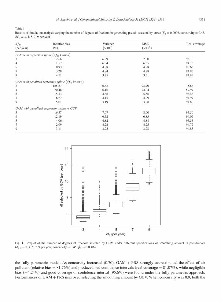
Table 1 reports the results of simulation analyses varying the number of degrees of freedom used to generate thepseudo-seasonality curve. Inference on � under fully parametric GAM+RS and semi-parametric GAM+PRS appeareddifferent. Even if the number of degrees of freedom used to fit the data was correctly specified, the estimator of � in thesemi-parametric model resulted strongly biased for high amounts of smoothing (relative bias = 155.57% for df 0 = 3per year, relative bias = 70.48% for df 0 = 4 per year). The bias decreased as df 0 increased. On the contrary, percentrelative bias under GAM + RS ranged from 0.93 to 4.11. Real coverage of the 95% confidence intervals was alwaysclose to 95% under GAM + RS, while it appeared very unsatisfactory under GAM + PRS, in particular for low valuesof df 0 (5.9% and 61.55% when df 0 = 3 and 4 per year, respectively).

Performances of semi-parametric model with smoothing parameter selected by GCV were comparable to the per-formances of the correctly specified GAM+RS in terms of coverage of confidence intervals and only moderate bias ofthe estimate of � was observed when a very smooth seasonality function was used to generate pseudo-data. It shouldbe noticed that the number of degrees of freedom selected by GCV, in this and all the following simulation analyses,was always higher than that used to generate the data (Fig. 1).

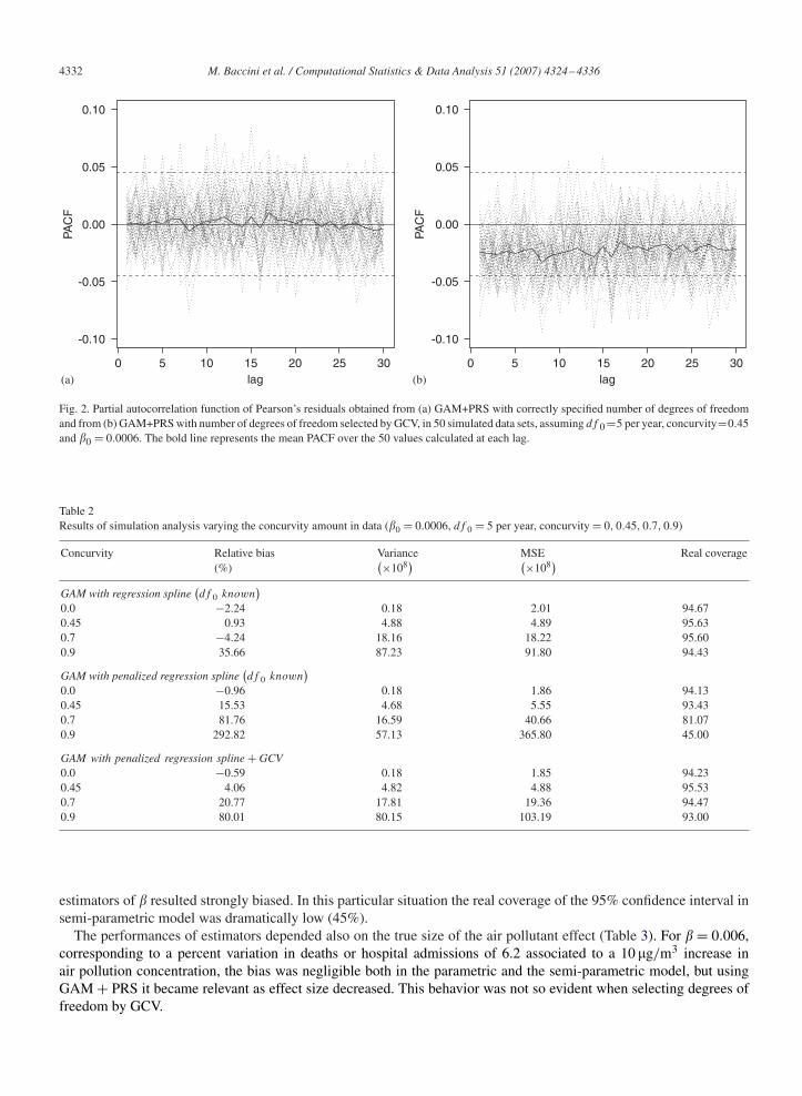
Minimizing GCV produced on average strongly negative partial autocorrelation function (PACF) of residuals. InFig. 2, we compare the PACFs of Pearson’s residuals obtained from (a) GAM+PRS with number of degrees of freedomcorrectly specified with (b) those obtained from GAM + PRS with number of degrees of freedom selected by GCV,in 50 simulated data sets, assuming 5 degrees of freedom per year, concurvity equal to 0.45 and effect size equal to0.0006. When the amount of smoothing was correctly specified, Pearson’s residuals appeared uncorrelated, despite thepoor performance of the air pollution effect estimator. On the contrary, negative autocorrelations were observed usingGCV, when the bias of the estimator for the air pollution parametric coefficient resulted negligible.

Summaries of results obtained varying the amount of concurvity in pseudo-data are reported in Table 2. In general,the bias increased as concurvity increased, but the size of bias depended on the modeling approach. When assigningdf 0 degrees of freedom to the spline (correct specification hypothesis), for a value of concurvity around 0.45, therelative bias of the estimator of air pollutant effect was 15.53% under the semi-parametric model and 0.93% under


Table 1Results of simulation analysis varying the number of degrees of freedom in generating pseudo-seasonality curve (�0 = 0.0006, concurvity = 0.45,df 0 = 3, 4, 5, 7, 9 per year)

df 0 Relative bias Variance MSE Real coverage(per year) (%)

(×108) (×108)

GAM with regression spline(df 0 known

)3 2.66 6.99 7.00 95.104 1.57 6.34 6.35 94.735 0.93 4.88 4.88 95.637 3.28 4.24 4.28 94.839 4.11 3.25 3.31 94.93

GAM with penalized regression spline(df 0 known

)3 155.57 6.63 93.70 5.864 70.48 6.16 24.04 59.975 15.53 4.68 5.56 93.437 6.27 4.15 4.29 94.979 5.01 3.19 3.28 94.80

GAM with penalized regression spline + GCV3 16.57 7.07 8.00 93.504 12.19 6.32 6.85 94.075 4.06 4.82 4.88 95.537 2.99 4.22 4.25 94.779 3.11 3.25 3.28 94.83

6

3 4 5 7 9

8

10

12

14

df0 (per year)

df s

elec

ted

by G

CV

(pe

r ye

ar)

Fig. 1. Boxplot of the number of degrees of freedom selected by GCV, under different specifications of smoothing amount in pseudo-data(df 0 = 3, 4, 5, 7, 9 per year, concurvity = 0.45, �0 = 0.0006).

the fully parametric model. As concurvity increased (0.70), GAM + PRS strongly overestimated the effect of airpollutant (relative bias = 81.76%) and produced bad confidence intervals (real coverage = 81.07%), while negligiblebias (−4.24%) and good coverage of confidence interval (95.6%) were found under the fully parametric approach.Performances of GAM + PRS improved selecting the smoothing amount by GCV. When concurvity was 0.9, both the


0 5 10 15 20 25 30

-0.10

-0.05

0.00

0.05

0.10

lag

PAC

F

-0.10

-0.05

0.00

0.05

0.10

PAC

F

0 5 10 15 20 25 30lag(a) (b)

Fig. 2. Partial autocorrelation function of Pearson’s residuals obtained from (a) GAM+PRS with correctly specified number of degrees of freedomand from (b) GAM+PRS with number of degrees of freedom selected by GCV, in 50 simulated data sets, assuming df 0 =5 per year, concurvity=0.45and �0 = 0.0006. The bold line represents the mean PACF over the 50 values calculated at each lag.

Table 2Results of simulation analysis varying the concurvity amount in data (�0 = 0.0006, df 0 = 5 per year, concurvity = 0, 0.45, 0.7, 0.9)

Concurvity Relative bias Variance MSE Real coverage(%)

(×108) (×108)


)0.0 −2.24 0.18 2.01 94.670.45 0.93 4.88 4.89 95.630.7 −4.24 18.16 18.22 95.600.9 35.66 87.23 91.80 94.43


)0.0 −0.96 0.18 1.86 94.130.45 15.53 4.68 5.55 93.430.7 81.76 16.59 40.66 81.070.9 292.82 57.13 365.80 45.00

GAM with penalized regression spline + GCV0.0 −0.59 0.18 1.85 94.230.45 4.06 4.82 4.88 95.530.7 20.77 17.81 19.36 94.470.9 80.01 80.15 103.19 93.00

estimators of � resulted strongly biased. In this particular situation the real coverage of the 95% confidence interval insemi-parametric model was dramatically low (45%).

The performances of estimators depended also on the true size of the air pollutant effect (Table 3). For � = 0.006,corresponding to a percent variation in deaths or hospital admissions of 6.2 associated to a 10 �g/m3 increase inair pollution concentration, the bias was negligible both in the parametric and the semi-parametric model, but usingGAM + PRS it became relevant as effect size decreased. This behavior was not so evident when selecting degrees offreedom by GCV.


Table 3Results of simulation analysis varying the air pollutant coefficient (df 0 = 5 per year, concurvity = 0.45, �0 = 0.0001, 0.0006, 0.006)

� Relative bias Variance MSE Real coverage(%)

(×108) (×108)


)0.0001 −5.51 5.07 5.08 95.470.0006 0.93 4.88 4.88 95.630.006 0.11 6.40 6.41 94.37


)0.0001 85.29 4.89 5.63 92.870.0006 15.53 4.68 5.55 93.430.006 1.12 6.31 6.76 92.90

GAM with penalized regression spline + GCV0.0001 14.04 5.04 5.06 95.170.0006 4.06 4.82 4.88 95.530.006 0.29 6.37 6.39 94.03

-0.0005

0.0000

0.0005

0.0010

0.0015

df (per year)

coef

f.

-0.0005

0.0000

0.0005

0.0010

0.0015

coef

f.

df (per year)(a) (b)3 4 5 6 7 8 9 10 11 12 13 3 4 5 6 7 8 9 10 11 12 13

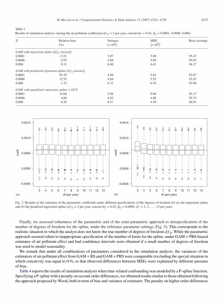
Fig. 3. Boxplot of the estimates of the parametric coefficient under different specifications of the degrees of freedom for (a) the regression splineand (b) the penalized regression spline (df 0 = 5 per year, concurvity = 0.45, �0 = 0.0006; df = 1, 2, . . . , 13 per year).

Finally, we assessed robustness of the parametric and of the semi-parametric approach to misspecification of thenumber of degrees of freedom for the spline, under the reference parameter settings (Fig. 3). This corresponds to therealistic situation in which the analyst does not know the true number of degrees of freedom df 0. While the parametricapproach seemed robust to inappropriate specification of the number of knots for the spline, under GAM + PRS biasedestimates of air pollutant effect and bad confidence intervals were obtained if a small number of degrees of freedomwas used to model seasonality.

We remark that under all combinations of parameters considered in the simulation analysis, the variances of theestimators of air pollutant effect from GAM+RS and GAM+PRS were comparable (excluding the special situation inwhich concurvity was equal to 0.9), so that observed differences between MSEs were explained by different amountsof bias.

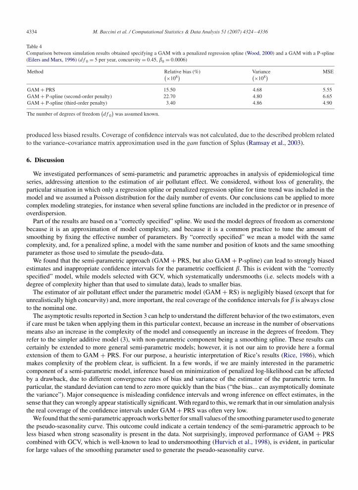
Table 4 reports the results of simulation analysis when time-related confounding was modeled by a P-spline function.Specifying a P-spline with a penalty on second-order differences, we obtained results similar to those obtained followingthe approach proposed by Wood, both in term of bias and variance of estimator. The penalty on higher order differences


Table 4Comparison between simulation results obtained specifying a GAM with a penalized regression spline (Wood, 2000) and a GAM with a P-spline(Eilers and Marx, 1996) (df 0 = 5 per year, concurvity = 0.45, �0 = 0.0006)

Method Relative bias (%) Variance MSE(×108) (×108)

GAM + PRS 15.50 4.68 5.55GAM + P-spline (second-order penalty) 22.70 4.80 6.65GAM + P-spline (third-order penalty) 3.40 4.86 4.90

The number of degrees of freedom(df 0

)was assumed known.

produced less biased results. Coverage of confidence intervals was not calculated, due to the described problem relatedto the variance–covariance matrix approximation used in the gam function of Splus (Ramsay et al., 2003).

6. Discussion

We investigated performances of semi-parametric and parametric approaches in analysis of epidemiological timeseries, addressing attention to the estimation of air pollutant effect. We considered, without loss of generality, theparticular situation in which only a regression spline or penalized regression spline for time trend was included in themodel and we assumed a Poisson distribution for the daily number of events. Our conclusions can be applied to morecomplex modeling strategies, for instance when several spline functions are included in the predictor or in presence ofoverdispersion.

Part of the results are based on a “correctly specified” spline. We used the model degrees of freedom as cornerstonebecause it is an approximation of model complexity, and because it is a common practice to tune the amount ofsmoothing by fixing the effective number of parameters. By “correctly specified” we mean a model with the samecomplexity, and, for a penalized spline, a model with the same number and position of knots and the same smoothingparameter as those used to simulate the pseudo-data.

We found that the semi-parametric approach (GAM + PRS, but also GAM + P-spline) can lead to strongly biasedestimates and inappropriate confidence intervals for the parametric coefficient �. This is evident with the “correctlyspecified” model, while models selected with GCV, which systematically undersmooths (i.e. selects models with adegree of complexity higher than that used to simulate data), leads to smaller bias.

The estimator of air pollutant effect under the parametric model (GAM + RS) is negligibly biased (except that forunrealistically high concurvity) and, more important, the real coverage of the confidence intervals for � is always closeto the nominal one.

The asymptotic results reported in Section 3 can help to understand the different behavior of the two estimators, evenif care must be taken when applying them in this particular context, because an increase in the number of observationsmeans also an increase in the complexity of the model and consequently an increase in the degrees of freedom. Theyrefer to the simpler additive model (3), with non-parametric component being a smoothing spline. These results cancertainly be extended to more general semi-parametric models; however, it is not our aim to provide here a formalextension of them to GAM + PRS. For our purpose, a heuristic interpretation of Rice’s results (Rice, 1986), whichmakes complexity of the problem clear, is sufficient. In a few words, if we are mainly interested in the parametriccomponent of a semi-parametric model, inference based on minimization of penalized log-likelihood can be affectedby a drawback, due to different convergence rates of bias and variance of the estimator of the parametric term. Inparticular, the standard deviation can tend to zero more quickly than the bias (“the bias... can asymptotically dominatethe variance”). Major consequence is misleading confidence intervals and wrong inference on effect estimates, in thesense that they can wrongly appear statistically significant. With regard to this, we remark that in our simulation analysisthe real coverage of the confidence intervals under GAM + PRS was often very low.

We found that the semi-parametric approach works better for small values of the smoothing parameter used to generatethe pseudo-seasonality curve. This outcome could indicate a certain tendency of the semi-parametric approach to beless biased when strong seasonality is present in the data. Not surprisingly, improved performance of GAM + PRScombined with GCV, which is well-known to lead to undersmoothing (Hurvich et al., 1998), is evident, in particularfor large values of the smoothing parameter used to generate the pseudo-seasonality curve.


An interesting aspect of the problem concerns the relation between bias of the estimator and amount of concurvityin the data. According to the asymptotic theory, the simulation studies showed that, if a semi-parametric model isspecified, inference on the air pollutant effect can strongly depend on concurvity. Other conditions being equal, the bias

is larger as the amount of concurvity is large and becomes negligible if concurvity is close to zero(E

(�̂ − �

)≈ B1

).

We found also that semi-parametric modeling works better when the effect to be detected is large. This relationbetween performances of the estimator of air pollutant effect from GAM + PRS and true effect size was also describedby Dominici et al. (2002).

Introduction of less stringent conditions on the spline coefficients, for example a penalty on third-order differences ina P-spline context (Table 4), appeared to have consequences that are similar to those of undersmoothing, in accordanceto Proposition D in Rice (1986).

Under the fully parametric model, no discrepancy is documented between convergence rates of variance and bias.Then, given the sample size, we expect smaller bias of the estimator under GAM + RS than under GAM + PRS andcomparable variances. Results of our simulation analysis confirmed this heuristic expectation, and, as a consequenceof comparability between convergence rates of bias and variance, we found that the real coverage of the confidenceintervals under the fully parametric GAM is always close to the nominal one.

These appealing findings about GAM + RS seem to remain valid even under misspecification of the number ofdegrees of freedom for the regression spline, as shown by the robustness analysis under a set of parameters chosen toreproduce a typical epidemiological time series context.

The reported results suggest the following conclusions. Modeling seasonality by penalized regression splines or,plausibly, by other non-parametric functions, such as smoothing splines or locally weighted regression smoothers,can provide biased estimates of air pollutant effect and misleading confidence intervals, mostly depending on factorswhich cannot be controlled (concurvity, effect size, seasonality pattern). A certain degree of undersmoothing can leadto better inference on the air pollutant effect. In this sense methods like GCV or AIC (Akaike, 1973), which tendto select small smoothing parameters, can improve inference. On the contrary, the appropriateness of inspection ofpartial autocorrelation of residuals, widely used to select smoothing amount in epidemiological time series analyses,is questionable.

The fully parametric approach is not affected by the same drawbacks as the semi-parametric approach; moreoverwe found that, at least in typical situations, it is robust to misspecification of the degrees of freedom for the seasonalregression spline. The robustness of inference on air pollutant effect with respect to smooth term specification is veryimportant from a practical point of view. In fact, frequently in epidemiological time series analysis, the number ofdegrees of freedom of the spline is not selected on the basis of GCV, AIC or other information criteria, but it is a priorifixed to guarantee that results deriving from different time series can be compared, usually for meta-analytic purposes.

However, since our robustness results refer to a particular set of parameters, in presence of strong concurvity or verysmall effect size, sensitivity analysis changing the number of knots is advisable.

One could object that GAM+RS could be sensitive to the placement of knots in the regression spline definition (Hastieand Tibshirani, 1990; Green and Silverman, 1994). Since time is an evenly spaced covariate (it indexes days understudy) and the number of knots is usually not small (more than 3–4 per year), we do not expect relevant differenceschanging knots positions. This point can be more critical if other regression splines (namely for temperature) areincluded in the model.

On the other side, a possible advantage of the penalized approach is that it deals much better with missing data(that we have not considered in our simulation), while the fully parametric specification could result in computationalproblems. Again, this is a general point the relevance of which is attenuated in this specific field, because data areusually pre-processed to replace missing values (e.g. in the air pollutant time series) and because of the regularity ofthe time covariate modeled by the smooth term.

Acknowledgements

The authors are grateful to the anonymous referees for their thorough and constructive review. The research waspartially supported by PRIN 2002134337, PRIN 2004137478 and European Union V Framework Programme PHEWEProject “Assessment and Prevention of acute Health Effects of Weather conditions in Europe” QLK4-CT-2001-00152.


References

Akaike, H., 1973. Information theory and an extension of the maximum likelihood principle. In: Petrov, B.N., Csaki, F. (Eds.), Proceeding of SecondInternational Symposium on Information Theory. Akadémiai Kiadò, Budapest, pp. 267–281.

Biggeri, A., Baccini, M., Accetta, A., Lagazio, C., 2002. Estimates of short-term effects of air pollutants in Italy. Epidemiol. Prev. 26, 203–205(in Italian).

Biggeri, A., Baccini, M., Bellini, P., Terracini, B., 2005. Italian studies of short term effect of air pollution (MISA), 1990–1999. Internat. J. Occup.Environ. Health 11, 107–122.

Cleveland, W.S., 1979. Robust locally weighted regression and smoothing scatterplots. J. Amer. Statist. Assoc. 74, 829–836.Currie, I.D., Durban, M., 2002. Flexible smoothing with P-splines: an unified approach. Statist. Modelling 4, 333–349.Daniels, M.J., Dominici, F., Samet, S., 2004. Underestimation of standard errors in multisites time series studies. Epidemiology 15, 57–62.de Boor, C., 1978. A Practical Guide to Splines. Springer, New York.Dominici, F., McDermott, A., Zeger, S.L., Samet, J., 2002. On the use of generalized additive models in time-series studies of air pollution and

health. Am. J. Epidemiol. 156, 193–203.Dominici, F., McDermott, A., Hastie, T., 2004. Improved semi-parametric time series models of air pollution and mortality. J. Amer. Statist. Assoc.

468, 938–948.Eilers, P.H.C., Marx, B.D., 1996. Flexible smoothing with B-splines and penalties (with discussion). Statist. Sci. 11, 89–121.Green, P.J., Silverman, B.W., 1994. Nonparametric Regression and Generalized Linear Models. Chapman & Hall, London.Hastie, T.J., Tibshirani, R.J., 1986. Generalized additive models. Statist. Sci. 1, 295–318.Hastie, T.J., Tibshirani, R.J., 1990. Generalized Additive Models. Chapman & Hall, London.Heckman, N.E., 1985. Spline smoothing in a partly linear model. J. Roy. Statist. Soc. B 48, 244–248.Hurvich, C.M., Simonoff, J.S., Tsai, C.L., 1998. Smoothing parameter selection in non-parametric regression using an improved Akaike information

criterion. J. Roy. Statist. Soc. B 60, 271–293.Kaiser, J., 2002. Software glitch threw off mortality estimates. Science 296, 1945–1946.Katsouyanni, K., Touloumi, G., Samoli, E., Gryparis, A., Le Tertre, A., et al., 2001. Confounding effect modification in the short-term effects of

ambient particles on total mortality: results from 29 European cities within the APHEA 2 project. Epidemiology 12, 521–531.Knight, J., 2002. Statistical error leaves pollution data in the air. Nature 417, 677.Lumley, T., Sheppard, L., 2003. Time series analyses of air pollution on health: straining at gnats and swallowing camels? Epidemiology 14, 13–14.Marx, B.D., Eilers, P.H.C., 1998. Direct generalized additive modeling with penalized likelihood. Comput. Statist. Data Anal. 28, 193–209.MathSoft Inc., 1999. Splus 2000 Professional Release 1. MathSoft Inc., Seattle, Washington.McCullagh, P., Nelder, J.A., 1989. Generalized Linear Models. second ed. Chapman & Hall, London.R Development Core Team, 2004. R: a Language and Environment for Statistical Computing. Vienna: R Foundation for Statistical Computing.

Available from 〈http://www.R-project.org〉.Ramsay, T.O., Burnett, R.T., Krewski, D., 2003. The effect of concurvity in generalized additive models linking mortality to ambient particulate

matter. Epidemiology 14, 18–23.Rice, J., 1986. Convergence rates for partially splined models. Statist. Probab. Lett. 4, 203–208.Ruppert, D., 2002. Selecting the number of knots for penalized splines. J. Comput. Graphical Statist. 11, 735–757.Ruppert, D., Carroll, R.J., 1997. Penalized regression splines. Working Paper, School of Operation Research and Industrial Engineering, Cornell

University.Ruppert, D., Wand, M.P., Carroll, R.J., 2003. Semiparametric Regression. Cambridge University Press, New York.Saez, M., Ballester, F., Barcelo, M.A., Perez-Hoyos, S., Bellido, J., et al., 2002. A combined analysis of the short-term effects of photochemical air

pollutants on mortality within the EMECAM project. Environ. Health Perspect. 110, 221–228.Samet, J.M., Zeger, S.L., Dominici, F., Curriero, F., Coursac, I., et al., 2000. The national morbidity, mortality, and air pollution study. Part II:

morbidity and mortality from air pollution in the United States (with discussion). Research Report of Health Effects Institute, vol. 94, pp. 5–79.SAS Institute Inc., 1999. SAS Procedures Guide, Version 8, SAS Institute Inc., Cary, NC.Saurina, C., Barcelo, M.A., Saez, M., Tobias, A., 1999. The short-term impact of air pollution on the mortality. Results of the EMECAM project in

the city of Barcelona, 1991–1995. Rev. Esp. Salud Publica 73, 199–207 (in Spanish).Schimek, M.G., 2000. Estimation and inference in partially linear models with smoothing splines. J. Statist. Plann. Inference 91, 525–540.Schimek, M.G., Turlach, B., 2000. Additive and generalized additive models. In: Schimek, M.G. (Ed.), Smoothing and Regression. Approaches,

Computation and Application. Wiley, New York, pp. 277–327.Schwartz, J., 1994. The use of generalized additive models in epidemiology. In: Proceedings of XVII International Biometric Society Conference,

Hamilton, Ontario, pp. 55–80.Speckman, P., 1988. Kernel smoothing in partial linear models. J. Roy. Statist. Soc. B 50, 413–436.The HEI Review Panel, 2003. Commentary to the Health Effects Institute. Revised analyses of time series studies of air pollution and health. Special

Report, Health Effects Institute, Boston, MA, pp. 255–271.Wood, S.N., 2000. Modelling and smoothing parameter estimation with multiple quadratic penalties. J. Roy. Statist. Soc. B 62, 413–428.Wood, S.N., 2001. mgcv: GAMs and Generalized Ridge Regression for R. R News, vol. 1, pp. 20–25.Wood, S.N., Augustin, N.H., 2002. GAMs with integrated model selection using penalized regression splines and applications to environmental

modelling. Ecol. Modelling 157, 157–177.

http://www.R-project.org

parametric and semi-parametric approaches in the analysis of short-term effects of air pollution on...

Documents