semi-parametric and parametric inference of extreme...

Water Resour Manage (2010) 24:1229–1249DOI 10.1007/s11269-009-9493-3

Semi-parametric and Parametric Inference of ExtremeValue Models for Rainfall Data

Amir AghaKouchak · Nasrin Nasrollahi

Received: 11 November 2008 / Accepted: 27 July 2009 /Published online: 7 August 2009© Springer Science+Business Media B.V. 2009

Abstract Extreme rainfall events and the clustering of extreme values providefundamental information which can be used for the risk assessment of extremefloods. Event probability can be estimated using the extreme value index (γ ) whichdescribes the behavior of the upper tail and measures the degree of extreme valueclustering. In this paper, various semi-parametric and parametric extreme valueindex estimators are implemented in order to characterize the tail behavior of long-term daily rainfall time series. The results obtained from different estimators are thenused to extrapolate the distribution function of extreme values. Extrapolation canbe employed to estimate the occurrence probability of rainfall events above a giventhreshold. The results indicated that different estimators may result in considerabledifferences in extreme value index estimates. The uncertainty of the extreme valueestimators is also investigated using the bootstrap technique. The analyses showedthat the parametric methods are superior to the semi-parametric approaches. Inparticular, the likelihood and Two-Step estimators are preferred as they are foundto be more robust and consistent for practical application.

Keywords Extreme rainfall · Extreme value index · Semi-parametric andparametric estimators · Generalized Pareto Distribution

A. AghaKouchakInstitute of Hydraulic Engineering, University of Stuttgart, Pfaffenwaldring 61, 70569,Stuttgart, Germany

A. AghaKouchak (B) · N. NasrollahiDepartment of Civil Engineering, University of Louisiana at Lafayette, PO Box 42291,Lafayette, LA 70504, USAe-mail: [email protected]

N. Nasrollahie-mail: [email protected]

1230 A. AghaKouchak, N. Nasrollahi

1 Introduction

The statistical analysis of extreme rainfall events is a prerequisite for water resourcesrisk assessment and decision making. Recent studies indicate changes in intensityand frequency of extremes across the globe (IPCC 2001, 2007; Kharin and Zwiers2000; Colombo et al. 1999; Goldstein et al. 2003). Changes in extreme climate events(e.g. extreme precipitation, floods, drought, etc.) are particularly important due totheir significant impacts on human livelihood and socio-economic developments. Inthe past twenty five years, five billion people were affected by natural disasters re-sulting in approximately $1 trillion in economic losses around the world (Stromberg2007). Floods, in particular, are the most life threatening hydrologic phenomenathat result in extensive property damage and loss of lives each year. Analysis ofextreme precipitation events may improve assessment of flood forecast which isinfluential in water resources management. By analyzing the trend in the annualprecipitation values, Karl et al. (1996) reported an increase in the frequency of highintensity precipitation events across the United States over the period of 1910 to1996. Kharin and Zwiers (2000) highlighted possible future changes in extremes ofdaily temperature and their effects on extreme precipitation events. Furthermore,several climate studies confirmed the importance of extreme precipitation events onassessment of the impact of potential climate change on the water balance and runoffprocesses (Abdulla et al. 2009; Iglesias et al. 2007; Xu et al. 2004; Göncü and Albek2009; Li et al. 2009).

Extreme Value Theory (EVT) is frequently used in water resources engineeringand management studies (Katz et al. 2002; Smith 2001; Coles 2001 and referencestherein) to obtain probability distributions to fit maxima or minima of data in randomsamples, as well as to model the distribution excess above a certain threshold. For thefirst time, Fisher and Tippett (1928) introduced the asymptotic theory of extremevalue distributions. Gnedenko (1943) provided mathematical proof to the factthat under certain conditions, three families of distributions (Gumbel, Fréchet andWeibull) can arise as limiting distributions of extreme values in random samples. Thecombination of Gumbel, Fréchet and Weibull families is known as the GeneralizedExtreme Value (GEV) distribution (Gumbel 1958; Smith 2001; Goldstein et al.2003). Based on this theory, Gumbel (1942) addressed frequency distribution ofextreme values in flood analysis. Gumbel (1958) further developed the GEV theoryand applied it for various practical applications. In hydrology literature, the GEVapproach is often referred to as the annual maxima or block maxima when it is usedto fit distributions to maxima/minima of a given dataset (Goldstein et al. 2003).

An alternative approach to the annual maxima is the so-called threshold methodwhich is based on exceedances above thresholds. The threshold approach is theanalog of the generalized extreme value distribution for the annual maxima, but itleads to a distribution called the Generalized Pareto Distribution (GPD) which isproven to be more flexible than the annual maxima (Smith 2001; Goldstein et al.2003; Smith and Shively 1995). One advantage of the threshold methods over theannual maxima is that they can deal with asymmetries in the tails of distributions(McNeil and Frey 2000).

The fundamentals of extreme value analysis based on threshold values wereestablished by Balkema and De Haan (1974) and Pickands (1975) whereby the

Semi-parametric and Parametric Inference of Extreme Value Models for Rainfall Data 1231

mean number of exceedances above a high threshold in a cluster was given asthe key parameter. Extreme event probability can be estimated using the extremevalue index (γ ) which describes the behavior of the upper tail and measures thedegree of clustering of extreme values. The rainfall extreme value index correspondsto the mean number of exceedances above a high threshold in a cluster, and canbe estimated using a limited sample from an unknown distribution. For practicalapplication of the GPD approach, the parameters are to be estimated first. Hill (1975)and Pickands (1975) introduced the Hill and the Pickands estimators respectively.Dekkers et al. (1989), Danielsson and Vries (1997) and Ferreira et al. (2003)proposed and applied different moment based estimators for the extreme valueindex. Landwehr et al. (1979) presented the Probability Weighted Moments (PWM)approach, that is linear combinations of L-moments (Hosking 1990), for parameterestimation of extreme value distributions. The L-moment theory offers a parameterestimation technique which is particularly used when the sample size is limited(Kharin and Zwiers 2000). Laurini and Tawn (2003) introduced a method knownas the two-threshold approach whereby the extreme value index is represented bythe number of independent clusters observed in the sample data. This method islimited in that it requires the preliminary identification of clusters, and the choiceof two declustering parameters. Zhou (2008) proposed a two-step scale invariantmaximum likelihood estimator of the extreme value index and Ferro and Segers(2003) adopted a moment-based estimator for high quantiles. However, the latteris not flexible in analyzing changes of the extreme value index over time. Lu andPeng (2003) developed an empirical likelihood method for the extreme value indexof heavy tailed distributions. In addition to the quantitative parameter estimationmethods, mentioned above, there are several graphical techniques such as thequantile-quantile (Q-Q) plot and probability plot correlation coefficient (PPCC) thatcan be used for data exploration and visual goodness-of-fit tests (Goldstein et al.2003).

Recently, application of extreme value theory has drawn the attention of hy-drologists for prediction of extreme events. Different longterm rain gauge andsurface runoff data have been investigated with respect to their extreme valuedistributions (see Pagliara et al. 1998; Bernardara et al. 2008; Withers and Nadarajah2000; Haylock and Nicholls 2000; Koutsoyiannis and Baloutsos 2000; Aronica et al.2002; Nguyen et al. 2002; Segal et al. 2002; Crisci et al. 2008; Shane and Lynn 1964;Todorovic and Zelenhasic 1970; Madsen et al. 1997a, b; Alila 1999; Fowler and Kilsby2003; Koutsoyiannis 2004; Semmler and Jacob 2004; Martins and Stedinger 2000;Morrison and Smith 2002; Glaves and Waylen 1997). For other applications of theextreme value theory in meteorology, oceanography and climatology the interestedreader is referred to Khaliq et al. (2005), van den Brink et al. (2004), Voss et al.(2002), van den Brink et al. (2003), Sánchez-Arcilla et al. (2008) and Galiatsatou et al.(2008). Ouarda et al. (1994) presented commonly used extreme value distributionsin hydrology based on the asymptotic behavior of their probability density functions.Egozcue and Ramis (2001) investigated heavy precipitation events across the easternSpain and reported heavy tailed distributions for the extremes. Buishand (1991)conducted analyses of precipitation extremes over regional scales. In general, theobjective of extreme rainfall analysis is to obtain reasonable estimates of extremerainfall quantiles which exceed a given threshold. As discussed previously, this can


be achieved by fitting the Generalized Pareto (GP) distribution to the excessesover a certain threshold. In this paper, different extreme value index estimators areimplemented in order to characterize the tail behavior of long-term daily rainfall timeseries. The results obtained from different estimators are then used to extrapolatethe distribution function of extreme values. Such extrapolation can be employedto estimate occurrence probability of rainfall above a certain threshold. In thisstudy, the uncertainty of the extreme value index estimators is investigated using thebootstrap technique (Efron 1979, 1981, 1987; Davison and Hinkley 1997; Carpenterand Bithell 2000; Shao and Tu 1995; Efron and Tibshirani 1997). This techniqueis a data-driven method that employs Monte Carlo simulations to draw randomsub-samples from the data under consideration in order to generate an empiricalestimate for the sampling distribution of a statistic (Qi 2008). The bootstrap hasbeen frequently used in practical applications for determining the accuracy (oruncertainty) of statistical analyses (Dunn 2001; Kharin and Zwiers 2000; Dixon 2002;Khaliq et al. 2005; Ferro and Segers 2003; Zwiers 1990; Zhang et al. 2005; Wilks 1997;Zwiers and Ross 1991).

The paper is divided into seven sections. After the introduction, the requiredtheoretical background to follow the subsequent sections is briefly reviewed. Thethird section discusses various extreme value index estimators. In the fourth section,properties and restrictions of the estimators are reviewed. The fifth section describesrainfall data and the study areas. The sixth section is devoted to the results anddiscussion whereas the last section summarizes the findings and conclusions.

2 Theoretical Background

Generally, the steps to analyze the tail behavior of extremes based upon the Gener-alized Pareto Distribution can be summarized after Pérez-Fructuoso et al. (2007): (1)Selecting a threshold over which the GPD is fitted. (2) Parameter estimation usingan extreme value index estimator which can reasonably model the tail behavior. (3)Evaluating the goodness of fit. (4) Performing the inference of extreme value models.This paper is devoted mainly to parameter estimation using various extreme valueindex estimators (step 2) and their associated uncertainties.

Theoretically, extreme value distributions are derived as limiting distributionsof large or small values in samples from random variables. Performing a lineartransformation in order to reduce the actual size of large (or small) values is essentialto obtain a non-degenerate limiting distribution (see Kotz and Nadarajah 2000).Keeping this in mind, let F be the distribution function of x1, x2...xn independent andidentically distributed (i.i.d.) random variables. For a non-degenerate distributionfunction G, an > 0 and b n ∈ � the following argument is valid:

G(x) = limn→∞ Fn(anx + b n) (1)

where an and b n may depend on the sample size but not on x. Equation 1 indicatesthat for all continuity points x of G, F ∈ D(G) (F is in the domain of attraction of thedistribution G) and thus, [G(x)]n = G(anx + b n). For a complete review and details,see: Qi (2008), Fisher and Tippett (1928), Galambos (1978) and Zhou (2008).


Different representations of an and b n result in various extreme-value distribu-tions. For example, the Gumbel distribution is obtained by assuming an = 1 whereasFréchet and negative Weibull are derived by taking an �= 1. For derivations, readersare referred to Qi (2008) and Galambos (1978). The behavior of extreme valuesare commonly described by the above mentioned distributions whose cumulativedistribution functions are displayed below:

G(x) = e−e(−x)

(2)

�(x) ={

0 x ≤ 0e−x−α

x > 0 and α > 0(3)

W(x) ={

e−(−x−α) x < 0 and α < 01 x ≥ 0

(4)

where: α = distribution parameterx = a sequence of independent and identically distributed (i.i.d)

random variables

The combination of the above distribution families is known as the generalizedextreme value (GEV) distribution that can be used to approximate the maxima offinite sequences of random variables. The standard cumulative distribution functionof the GEV can be expressed as:

�(x) = exp

{−

(1 + γ

(x − μ

σ

))− 1γ

}(5)

where: μ = location parameterσ = scale parameterγ = shape parameter

The extreme value index (γ ), also known as the shape parameter, governs the tailbehavior of the GEV distribution. The function �(x) is defined for 1 + γ

( x−μ

σ

)> 0;

elsewhere, the function �(x) is either 0 or 1 (Smith 2001). This implies, for γ > 0 orγ < 0, the density function has zero probability above (below) the upper (lower)bound defined as −1/γ . In the limit as γ approaches 0, the GEV distribution isunbounded. In Eq. 5, γ = 0, γ < 0 and γ > 0 represent the Gumbel, Weibull (withα = 1/γ ) and Fréchet (with α = 1/γ ) families, respectively. In the GEV distribution,if the γ > 0, the distribution is heavy tailed. The standard form of the GEV (Gγ (x) =e−(1+γ x)

− 1γ ) can be obtained by substituting μ = 0 and σ = 1 into Eq. 5.

Note that the mean and standard deviation of the GEV distribution exist if γ < 1and γ < 1/2, respectively (Smith 2001):

MX = E(X) = μ − σ

γ+ σ

γ(�(1 − γ )) (6)

SX =√

E(X − MX)2 = σ

γ

√(�(1 − 2γ ) − �2(1 − γ )

)(7)


where MX(γ < 1) and SX(γ < 1/2) are the mean and standard deviation. Equa-tions 6 and 7 can be extended to the fact that the nth moment of the GEV distributionexists if γ < 1/n. In subsequent sections, based upon the above formulation andconditions, various extreme value index estimators are reviewed and applied forrainfall data.

3 Estimation of the Extreme Value Index

There are generally two types of extreme value index estimators: (1) parametricsuch as the Maximum Likelihood, Probability Weighted Moment, Two-Step andThree-Step estimators; (2) semi-parametric such as the Pickands, Hill and Momentestimators. The main assumption behind parametric estimators is that the datafollows an exact GEV probability distribution function, defined by a number ofparameters. Semi-parametric estimators, however, are based on partial properties ofthe underlying distribution function. In the following, extreme value index estimatorsused in this study are described in details.

3.1 Pickands Estimator

Assume a finite sample of x1, x2...xn from a sequence of i.i.d. random variablessatisfying Eq. 1 is observed. Let xn,1 ≤ xn,2 ≤ ... ≤ xn,n be the ranking order ofx1, x2...xn. Then, xn,n − xn,n−k, ..., xn,n−k+1 − xn,n−k is the excess above the thresholdwhere k denotes the rank of the upper threshold. Pickands (1975) introduced anestimator for the extreme value index as follows:

γP = (log2)−1 log

(xn,n−k/4 − xn,n−k/2

xn,n−k/2 − xn,n−k

)(8)

3.2 Hill Estimator

Using the maximum likelihood approach and the excess ratios (xn,n/xn,n−k, ...,

xn,n−k+1/xn,n−k) instead of the excess above the threshold (as mentioned in PickandsEstimator), Hill (1975) proposed the following estimator for γ > 0:

γH = k−1k∑

i=1

log(xn,n−i+1 − xn,n−k

)(9)

where: k = rank of the upper threshold

The Hill estimator is based on the asymptotic behavior of the largest orderstatistics (Hill 1975) and is commonly used on practical applications (e.g. Casson andColes 1999; Brutsaert and Parlange 1998).


3.3 Moment Estimator

Dekkers et al. (1989) presented a more generalized estimator for γ ∈ � known as theMoment estimator:

γM = k−1k∑

i=1

log(xn,n−i+1 − xn,n−k

)

+1 − 1

2

⎛⎜⎝1 −

(k−1 ∑k

i=1 log(xn,n−i+1 − xn,n−k

))2

k−1∑k

i=1 log(xn,n−i+1 − xn,n−k

)2

⎞⎟⎠

−1

(10)

3.4 Probability Weighted Moment Estimator

By assigning different weighting factors to the excesses above the threshold, Hoskingand Wallis (1987) suggested the probability weighted moment estimator:

γW M = k−1 ∑k−1i=0 (xn,n−i − xn,n−k) − 4k−1 ∑k−1

i=0ik

(xn,n−i − xn,n−k

)k−1

∑k−1i=0 (xn,n−i − xn,n−k) − 2k−1

∑k−1i=0

ik


) (11)

3.5 Maximum Likelihood Estimator

Smith (1987) employed the maximum likelihood method to estimate γ ∈ �. Forthe case, γ �= 0 the maximum likelihood estimator can be expressed by solving thefollowing two equations:

γMLE = k−1k−1∑i=0

log(

1 + γMLE

σ


)),

1

1 + γMLE= k−1

k−1∑i=0

1

1 + γMLEσ


) (12)

where: σ = extreme value scaleNote that in the estimation of extreme quantiles of the GEV distribution, the

likelihood estimator is not reliable for small sample sizes (Hosking and Wallis 1987).This issue is further discussed in Section 4.

3.6 Two-Step Estimator

Zhou (2008) suggested the Two-step estimator as an approximation to the likelihoodformulation. The main motivation for this approach is based upon the fact that thereis no general explicit formulation for the likelihood estimator. In this approach, the


extreme value index is pre-estimated in the first step using, say, Pickands estimator.In the second step, an approximation to the likelihood function is performed suchthat the difference between the Two-step and likelihood estimators tend to zero. Forproof and details, readers are referred to Zhou (2008).

γ2S = 2γP + 1

2

W M2

(W M1

)2 − 1 (13)

where:

W M j =k∑

i=1

wji

(xn,n−i+1 − xn,n−k

) j, j = 1, 2 (14)

and

wji = 1

jγP + 1

((ik

) jγP+1

−(

i − 1

k

) jγP+1)

, j = 1, 2 (15)

3.7 Three-Step Estimator

By taking the final result of the Two-Step estimator and assuming it to be the firstestimate of the above procedure, Zhou (2008) proposed the Three-Step estimator,requiring one more iteration (the same as the Two-Step approach) to obtain theextreme value index.

4 Estimator Properties

There are a number of extreme value index estimators, commonly used in practicalapplications, but few are both shift and scale invariant (Aban and Meerschaert 2001).A shift invariant estimator is analogous to a time-invariant function; defined suchthat if z(x) = y(x), then z(x + t) = y(x + t) where t is the time shift (Kahvec et al.2001; Oppenheim and Schafer 1975). An estimator z(x) is said to be scale-invariantwhen multiplication of all elements of the sample (x1, ..., xn) by an arbitrary non-negative value β results in multiplication of the estimator by the same value (βz(x)).Table 1 summarizes the properties of introduced extreme value index estimators. Asindicated, The Moment and Hill estimators are both scale invariant; however, theyare not shift invariant. Hence, for improperly centered data, using these estimatorsmay result in misleading estimates of γ (Aban and Meerschaert 2001). Contrary to

Table 1 Properties of theextreme value indexestimators

EVI estimator Scale invariant Shift invariant Restriction

Pickands Yes Yes –Hill Yes No γ > 0Moment Yes No –PWM Yes Yes γ < 1/2Likelihood Yes Yes γ > −1/2Two-step Yes Yes –Three-step Yes Yes –


the moment and Pickands estimators which are consistent for all real values of γ , theHill estimator is restricted to γ > 0 .

The Probability Weighted Moment and likelihood estimators are both scale andshift invariant and are defined and consistent for γ < 1/2 and γ > −1/2, respectively.As previously mentioned, there is no general explicit formulation for the likelihoodestimator and it may not even exist (Zhou 2008). This problem is addressed in theTwo-Step estimator which is scale and shift invariant, and provides an approximationto the likelihood approach. The Three-Step procedure, similar to the Two-Stepestimator, is scale and shift invariant (Zhou 2008).

As mentioned before, the likelihood estimator is not reliable for small samplesizes. Martins and Stedinger (2000) demonstrated this issue by estimating the para-meter γ for a random sample (n = 15), generated from a GEV distribution with adefined γ . They showed that for such a small sample size, utilization of the maximumlikelihood estimator may lead to erroneous estimates of the extreme value index.Hosking et al. (1985) showed that the PWM estimator performs better than themaximum likelihood method in estimating upper quantiles of the GEV distributionwhen the sample size is small. Based on this reason, Hosking (1990) argued that thePWM estimator is superior to the maximum likelihood estimators.

Application of different estimators on real data may result in considerable dis-crepancies between estimated extreme value indices. Unfortunately, there is to-date no single estimator which has proved to be consistent and reliable under allcircumstances. This means that the choice of the proper estimator is somewhat data-dependent. Nevertheless, there are a number of issues that are discussed in Section 6.

5 Rainfall Data

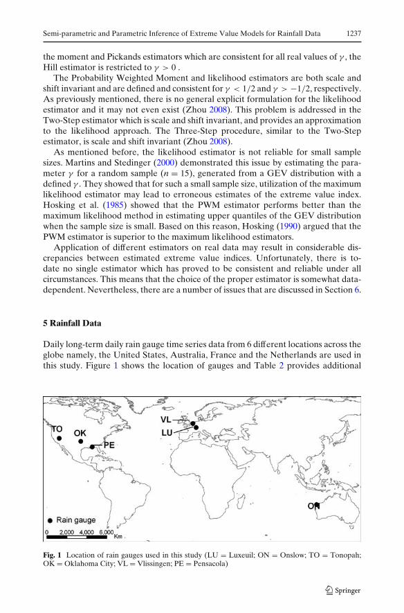
Daily long-term daily rain gauge time series data from 6 different locations across theglobe namely, the United States, Australia, France and the Netherlands are used inthis study. Figure 1 shows the location of gauges and Table 2 provides additional

Fig. 1 Location of rain gauges used in this study (LU = Luxeuil; ON = Onslow; TO = Tonopah;OK = Oklahoma City; VL = Vlissingen; PE = Pensacola)


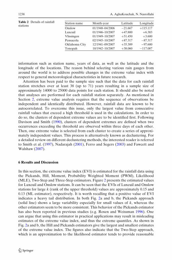
Table 2 Details of rainfallstations

Station name Month-year Latitude Longitude

Onslow 01/1948–04/2006 −21.667 +115.117Luxeuil 01/1946–10/2007 +47.800 +6.383Vlissingen 01/1949–10/2007 +51.450 +3.600Pensacola 02/1945–10/2007 +87.317 −87.317Oklahoma City 12/1941–09/2007 +35.389 −97.600Tonopah 10/1942–10/2007 +38.060 −117.087

information such as station name, years of data, as well as the latitude and thelongitude of the locations. The reason behind selecting various rain gauges fromaround the world is to address possible changes in the extreme value index withrespect to general meteorological characteristics in future research.

Attention has been paid to the sample size such that the data for each rainfallstation stretches over at least 38 (up to 71) years resulting in a sample size ofapproximately 14000 to 25000 data points for each station. It should also be notedthat analyses are performed for each rainfall station separately. As mentioned inSection 2, extreme value analysis requires that the sequence of observations beindependent and identically distributed. However, rainfall data are known to beautocorrelated. To overcome this issue, only the largest value from consecutiverainfall values that exceed a high threshold is used in the calculations. In order todo so, the clusters of dependent extreme values are to be identified first. FollowingDavison and Smith (1990), clusters of dependent extremes are defined when twooccurrences exceeding the threshold are observed within three days of each other.Then, one extreme value is selected from each cluster to create a series of approxi-mately independent values. This process is alternatively known as declustering. Fora detailed review on different declustering methods, the interested reader is referredto Smith et al. (1997), Nadarajah (2001), Ferro and Segers (2003) and Fawcett andWalshaw (2007).

6 Results and Discussion

In this section, the extreme value index (EVI) is estimated for the rainfall data usingthe Pickands, Hill, Moment, Probability Weighted Moment (PWM), Likelihood(MLE), Two-Step and Three-Step estimators. Figure 2 presents the estimated valuesfor Luxeuil and Onslow stations. It can be seen that the EVIs of Luxeuil and Onslowstations for large k (rank of the upper threshold) values are approximately 0.15 and0.13 (ML estimator), respectively. It is worth recalling that a positive value of EVIindicates a heavy tail distribution. In both Fig. 2a and b, the Pickands approach(solid line) shows a large variability especially for small values of k, whereas theother estimators seem to be more consistent. This behavior of the Pickands estimatorhas also been reported in previous studies (e.g. Rosen and Weissman 1996). Onecan argue that using this estimator in practical applications may result in misleadingestimates of the extreme value index, and thus the extreme quantiles. As shown inFig. 2a and b, the Hill and Pickands estimators give the largest and smallest estimatesof the extreme value index. The figures also indicate that the Two-Step approach,which is an approximation to the likelihood estimator tends to provide reasonable


Fig. 2 Estimated EVIs forLuxeuil and Onslow stations:γP (solid line), γH (dashedline), γM (diamond mark),γPWM (x-mark), γMLE(dashdot line), γ2P (o-mark),γMLE (dotted line) (a, b)

(a)

(b)

estimates often having a smoother trend. In both figures, the Two-Step (o-marked)and Three-Step (dotted line) are almost identical. This is due to the fact that theThree-Step approach follows the same mathematical formulation as that of the Two-Step with one more iteration in order to obtain the extreme value index.

Having estimating the GEV parameters, one can estimate the occurrence prob-ability of extreme rainfall values. Figure 3a and b display the so-called exponentialplot (Chambers 1977) for Luxeuil and Onslow stations. More precisely, the graphsshow observed and estimated (extrapolated based on the fitted GEV distribution)rainfall data versus the negative logarithm of the tail distribution (− ln(1 − �(x))).Practically, this plot can be used to determine the occurrence probability of rainfallabove a certain threshold (1/ex). The graph is known as the exponential plot because it converges to a straight line when γ approaches zero, resembling exponentialbehavior (Bernardara et al. 2008). For lower-bounded (heavy tail) distributions


Fig. 3 Extrapolation of theextreme value distribution forLuxeuil and Onslow stationsusing the hill (plus mark),moment (x-mark) andtwo-step (dotted line)estimators (a, b)

(a)

(b)

(γ > 0), the exponential plot grows faster than a straight line and bends toward upat larger values. In Fig. 3a and b, the increasing trend of the graphs reflect heavy tailbehavior for the underlying probability distributions. In the figures, the estimatedrainfall values, obtained based on the Hill (plus-marked), Tow-Step (x-marked) andMoment (dotted line) estimators are presented. The Hill approach seems to followthe trend of larger values, while the Two-Step method models the entire data set.The results of the Maximum Likelihood and Three-Steps are not included as theyare very similar to the Two-Step estimator.

Figure 4a and b present γ versus k values for Tonopah and Oklahoma Citystations, respectively. In both figures, the EVIs tend to zero for large values of k thatsuggest weaker tails than those of Luxeuil and Onslow (see Fig. 2). Figure 5a and bdisplay the exponential plot of the observe and estimated rainfall data for Tonopahand Oklahoma City stations. As shown, the graphs converge to straight lines. This


Fig. 4 Estimated EVIs forOklahoma City and Tonopahstations: γP (solid line), γH(dashed line), γM (diamondmark), γPWM (x-mark), γMLE(dashdot line), γ2P (o-mark),γMLE (dotted line) (a, b)

(a)

(b)

indicates that the fitted GEV distribution is unbounded. Recall that in the limits, as γ

approaches zero the GEV distribution is unbounded. The graphs show that when theextreme value index approaches zero, the occurrence probability of rainfall above acertain threshold increases almost linearly with respect to rain rate.

Figure 6a and b plot the extreme value index versus k for Vlissingen andPensacola stations, respectively. Estimated extreme value indices for large k valuesare γ = −0.07 (ML estimator) for Vlissingen and γ = −0.08 (ML estimator) forthe Pensacola station. A negative value for γ suggests that the distribution hasa finite right end-point. Notice that the Hill estimator always yields a positive γ

even if the distribution has a right end-point. In such case the Hill estimator mustbe discarded. Extrapolation of the fitted distribution functions for Vlissingen andPensacola stations are presented in Fig. 7a and b. As shown, for negative values of γ ,the estimated rainfall values grow slower than a straight line and bend toward downat larger values. It is noted that in Figs. 3, 5 and 7, the estimated rainfall values are


Fig. 5 Extrapolation of theextreme value distribution forOklahoma City and Tonopahstations using the hill (plusmark), moment (x-mark) andtwo-step (dotted line)estimators (a, b)

(a)

(b)

based on the k values that correspond to the 98th percentile of the observations ineach station.

In practical applications, an appropriate estimator may be selected according togoodness-of-fit tests or other statistical tools rather than on theoretical considera-tions. Therefore, an important step in the process of estimator identification is totest whether the resulting model fits the observations. Table 3 lists the root meansquared error (RMSE) values for different estimators based on the 98th percentileof the observations as the threshold in each station. In all cases, the likelihood andTwo-Step estimators resulted in the least RMSE values. One can see that there areconsiderable differences between the RMSE values of different estimators exceptfor Onslow station where the Moment, PWP, MLE and Two-Step estimators werefound to be equally good. Furthermore, the table clearly indicates that the Pickandsestimator is inferior to the other estimators.


Fig. 6 Estimated EVIs forVlissingen and Pensacolastations: γP (solid line), γH(dashed line), γM (diamondmark), γPWM (x-mark), γMLE(dashdot line), γ2P (o-mark),γMLE (dotted line) (a, b)

(a)

(b)

To evaluate the uncertainty of the extreme value index estimators, discussedin this study, the bootstrap technique (Efron 1979; Davison and Hinkley 1997;Carpenter and Bithell 2000) is performed as follows. For each rainfall station, 1000subsets of the original dataset is randomly selected such that each randomly selectedsubset contains 25% of the original sample size. The process is repeated for 50% and75% of the original dataset. For each randomly selected sub-sample, the extremevalue index is estimated using the estimators discussed in this paper. The meanabsolute error (MAE) of the estimated extremal indices obtained from the randomsub-samples are then calculated with respect to the extreme value index obtainedfrom the original dataset. The mean absolute error which is a quantity often usedto measure how close simulations (here, estimates from the random sub-samples)are to the observations (here, estimates from the original dataset) is defined as:MAE = 1

n

∑ni=1 |γSi − γOi|, where γSi and γOi represent extremal indices from sim-

ulated and observed datasets, and n is the number of pairs (Cox and Hinkley 1974;


Fig. 7 Extrapolation of theextreme value distribution forVlissingen and Pensacolastations using the moment(x-mark) and two-step (dottedline) estimators (a, b)

(a)

(b)

Bernardo and Smith 2000). Table 4 summarizes the MAE values of the estimatedextreme value indices for Luxeuil, Tonopah and Vlissingen stations. One can seethat for the largest sample size (75%), the ML estimator led to the least meanabsolute error (compare columns 4, 7 and 10 in Table 4). For the smallest sample size(25%), on the other hand, the Two-Step estimator for Luxeuil and Vlissingen stations

Table 3 RMSE of the fittedmodels (LU = Luxeuil;ON = Onslow; TO =Tonopah; OK = OklahomaCity; VL = Vlissingen;PE = Pensacola)

EVI estimator LU ON TO OK VL PE

Pickands 0.64 0.36 0.53 0.68 0.39 0.72Hill 0.24 0.38 0.30 0.61 N/A N/AMoment 0.29 0.21 0.35 0.33 0.28 0.38PWM 0.31 0.21 0.32 0.31 0.27 0.38Likelihood 0.22 0.21 0.29 0.27 0.19 0.36Two-step 0.20 0.21 0.22 0.27 0.19 0.38


Table 4 MAE values of the estimated extreme value indices from different estimators (LU =Luxeuil; TO = Tonopah; VL = Vlissingen)

EVI estimator LU TO VL

25% 50% 75% 25% 50% 75% 25% 50% 75%

Pickands 0.129 0.112 0.103 0.110 0.108 0.063 0.110 0.099 0.048Hill 0.077 0.037 0.022 0.054 0.036 0.026 N/A N/A N/AMoment 0.067 0.048 0.035 0.051 0.054 0.022 0.073 0.060 0.024PWM 0.066 0.060 0.028 0.064 0.056 0.019 0.069 0.055 0.020Likelihood 0.090 0.040 0.020 0.033 0.020 0.018 0.051 0.011 0.007Two-step 0.062 0.051 0.024 0.040 0.024 0.019 0.043 0.014 0.008

and the ML estimator for Tonopah station resulted in the least uncertainty in theestimated values. Overall, the table indicates that the ML and Two-Step estimatorsare subject to less variability.

7 Summary and Conclusions

The primary goal of this research was to investigate different extreme value index es-timators as they are important for assessing risk for extreme rainfall events and thusfloods. Different parametric and semi-parametric EVI estimators were employedin this study. The results showed that the semi-parametric Pickands approach wassubject to large variability especially for small values of k while the other estimatorsseemed to be more consistent. Additionally, Pickands estimated the smallest extremevalue index in most cases whereas Hill estimator provided the largest estimates ofEVI.

The maximum likelihood, Two-Step and Three-Step methods were generallysimilar as they follow similar mathematical formulation. The Two-Step approach,known as an approximation to the likelihood estimator, provided robust estimatesof the extreme value index for a wide range of k. The results shown in Figs. 2, 4and 6 indicated that the outputs of the Two-Step and Three-Step were very sim-ilar although the Tree-Step takes an additional iteration in order to improve theaccuracy. The Moment, PWM and ML estimators were robust at large k values butoften inconsistent at small k-s. Overall, the parametric Two-Step and ML estimatorswere preferred over the semi-parametric Pickands and Hill estimators due to theirrobustness and consistency. The Two-Step was also given priority over the otherparametric estimators for its stable performance for different values of k.

Attention must be paid to estimator characteristics and restrictions before anypractical application. The Moment and Hill estimators are both scale invariant;however, they are not shift invariant. Contrary to the moment and Pickands esti-mators which are consistent for all real values of γ , the Hill estimator is restricted toγ > 0. The Probability Weighted Moment and likelihood estimators are both scaleand shift invariant, and they are defined and consistent for γ < 1/2 and γ > −1/2,respectively.

Having estimated the extreme value index using different estimators, the distribu-tion function of extreme values was extrapolated using Generalized Extreme ValueDistribution. Such extrapolation can be employed to estimate occurrence probabilityof rainfall above a certain threshold. In cases where γ found to be positive, the Hill


approach seemed to follow the trend of larger values whereas the Two-Step methodtended to model the entire data set. In other words, a few very large values at thetail may affect the Hill estimates more than the Two-Step estimates. In Fig. 5a, forexample, one can see that the Hill estimator gives larger values, perhaps because ofthe upper few points that bend toward up. On the other hand, in Fig. 5b, where theupper few points bend toward down, the Hill estimator gives smaller values than theTwo-Step estimator. However, this cannot be simply generalized and more in-depthresearch is required to evaluate the sensitivity of the EVI estimators to the extremesand outliers.

The uncertainty of the extreme value models is addressed using the bootstraptechnique. Randomly selected subsets (1000 realizations) of the original dataset areused to estimate the extreme value index. Different sample sizes of 25%, 50% and75% of the original dataset were used to evaluate the uncertainty with respect to thesample size. The mean absolute error (MAE) of the estimated extremal indices, esti-mated for the random sub-samples, are then calculated and compared to the extremevalue index obtained from the original dataset. The results showed that, the ML andTwo-Step estimators led to the least uncertainty in the estimated extremal indicesfor different sub-samples. On the other hand, the Pickands estimator exhibited thehighest variability in the estimated extremal indices.

The results of this paper confirmed that different estimators may result inconsiderable differences in extreme value index estimates. Obviously, occurrenceprobability of extreme events as well as return level estimations strongly dependon γ and thus the choice of extreme value index estimator. While the choice ofestimator may be somewhat data dependent, the results of this study showed thatthe parametric estimators are superior to the semi-parametric ones. In particular,the ML and Two-Step estimators seem to be more robust and consistent for practicalapplication.

Acknowledgements The authors would like to express their gratitude to J. Tuhtan who has givenso generously of his time reviewing this manuscript and offering suggestions for improvement.Appreciation is expressed to the Associate Editor and anonymous reviewers for their constructivecomments which have led to substantial improvements in the final version of this paper.

References

Aban I, Meerschaert M (2001) Shifted hill’s estimator for heavy tails. Commun Stat Simul Comput30:949–962

Abdulla F, Eshtawi T, Assaf H (2009) Assessment of the impact of potential climate change on thewater balance of a semi-arid watershed. Water Resour Manag 23(10):2051–2068

Alila Y (1999) A hierarchical approach for the regionalization of precipitation annual maxima.Canada J Geophys Res 104(31):645–655

Aronica G, Cannarozzo M, Noto L (2002) Investigating the changes in extreme rainfall seriesrecorded in an urbanised area. Water Sci Technol 45:49–54

Balkema A, De Haan L (1974) Residual life time at great age. Ann Probab 2:792–804Bernardara P, Schertzer D, Sauquet E, Tchiguirinskaia I, Lang M (2008) The flood probability

distribution tail. Stoch Environ Res Risk Assess 22:107–122Bernardo J, Smith A (2000) Bayesian theory. Wiley, New Yorkvan den Brink H, Koennen G, Opsteegh J (2003) The reliability of extreme surge levels, estimated

from observational records of order hundred years. J Coast Res 19:376–388van den Brink H, Koennen G, Opsteegh J (2004) Statistics of synoptic-scale wind speeds in ensemble

simulations of current and future climate. J Climate 17:4564–4574


Brutsaert W, Parlange M (1998) Hydrologic cycle explains the evaporation paradox. Nature396(30):30

Buishand T (1991) Extreme rainfall estimation by combining data from several sites. Hydrolog Sci J36:345–365

Carpenter J, Bithell J (2000) Bootstrap confidence intervals: when, which, what? A practical guidefor medical statisticians. Stat Med 19:1141–1164

Casson E, Coles S (1999) Spatial regression models for extremes. Extremes 1:449–468Chambers J (1977) Computational methods for data analysis. Wiley, New YorkColes S (2001) An introduction to statistical modeling of extreme values. Springer, LondonColombo A, Etkin D, Karney B (1999) Climate variability and the frequency of extreme temperature

events for nine sites across Canada: implications for power usage. J Climate 12:2490–2502Cox D, Hinkley D (1974) Theoretical statistics. Chapman & Hall, LondonCrisci A, Gozzini B, Meneguzzo F, Pagliara S, Maracchi G (2008) Extreme rainfall in a changing

climate: regional analysis and hydrological implications in Tuscany. Hydrol Process 16:1261–1274Danielsson J, Vries C (1997) Tail index and quantile estimation with very high frequency data. J

Empir Finance 4:241–257Davison A, Hinkley D (1997) Bootstrap methods and their application. Cambridge University Press,

Cambridge, 592 ppDavison A, Smith R (1990) Models for exceedances over high thresholds (with discussion). JR Stat

Soc 52:393–442Dekkers A, Einmahl J, de Haan L (1989) A moment estimator for the index of an extremevalue

distribution. Ann Stat 17:1833–1855Dixon R (2002) Bootstrap resampling. In: El-Shaarawi AH, Piegorsch WW (eds) The encyclopedia

of environmetrics. Wiley, New York, pp 212–219Dunn P (2001) Bootstrap confidence intervals for predicted rainfall quantiles. Int J Climatol 21:89–94Efron B (1979) Bootstrap methods: another look at the jackknife. Ann Stat 7:1–26Efron B (1981) Censored data and the bootstrap. J Am Stat Assoc 76:312–319Efron B (1987) Better bootstrap confidence intervals. J Am Stat Assoc 82:171–200Efron B, Tibshirani R (1997) An introduction to the bootstrap. Chapman and Hall, London, 436 ppEgozcue J, Ramis C (2001) Bayesian hazard analysis of heavy precipitation in eastern Spain. Int J

Climatol 21:1263–1279Fawcett L, Walshaw D (2007) Improved estimation for temporally clustered extremes. Environ-

metrics 18(2):173–188Ferreira A, de Haan L, Peng L (2003) On optimising the estimation of high quantiles of a probability

distribution. Statistics 37(5):401–434Ferro C, Segers J (2003) Inference for clusters of extreme values. J R Stat Soc Ser B Stat Methodol

65:545–556Fisher R, Tippett L (1928) Limiting forms of the frequency distribution of the largest or smallest

member of a sample. Proc Camb Philos Soc 24:180–190Fowler H, Kilsby C (2003) A regional frequency analysis of United Kingdom extreme rainfall from

1961 to 2000. Int J Climatol 23:1313–1334Galambos J (1978) Which Archimedean copula is the right one? Wiley, New YorkGaliatsatou P, Prinos P, Sánchez-Arcilla A (2008) Estimation of extremes: conventional versus

Bayesian techniques. J Hydraul Res 46(2):211–223Glaves R, Waylen P (1997) Regional flood frequency analysis in southern Ontario using l-moments.

Can Geogr 41:178–193Gnedenko B (1943) Sur la distribution limite du terme maximum d’une série aléatoire. Ann Math

44:423–453Goldstein J, Mirza M, Etkin D, Milton J (2003) Hydrologic assessment: application of extreme value

theory for climate extreme scenarios construction. In: 14th symposium on global change andclimate variations, American meteorological society 83rd annual meeting, Long Beach, 9–13 Feb2003

Göncü S, Albek E (2009) Modeling climate change effects on streams and reservoirs with hspf. WaterResour Manag. doi:10.1007/s11269–009–9466–6

Gumbel E (1942) On the frequency distribution of extreme values in meteorological data. Bull AmMeteorol Soc 23:95–104

Gumbel E (1958) Statistics of extremes. Columbia University Press, New YorkHaylock M, Nicholls N (2000) Trends in extreme rainfall indices for an updated high quality data set

for australia. Int J Climatol 20:1533–1541

http://dx.doi.org/10.1007/s11269--009--9466--6


Hill B (1975) A simple general approach to inference about the tail of a distribution. Ann Stat 3:1163–1174

Hosking J (1990) L-moments: analysis and estimation of distributions using linear combinations oforder statistics. J Royal Stat Soc Ser B 52:105–124

Hosking J, Wallis J (1987) Parameter and quantile estimation for the generalized pareto distribution.Technometrics 29:339–349

Hosking J, Wallis J, Wood E (1985) Estimation of the generalised extreme-value distribution by themethod of probabilityweighted moments. Technometrics 27:251–261

Iglesias A, Garrote L, Flores F, Moneo M (2007) Challenges to manage the risk of water scarcity andclimate change in the mediterranean. Water Resour Manag 21(5):775–788

IPCC (2001) Climate change 2001: impacts, adaptation, and vulnerability. In: McCarthy JJ, CanzianiOF, Leary NA, Dokken DJ, White KS (eds) Contribution of working group II to the thirdassessment report of the intergovernmental panel on climate change. Cambridge UniversityPress, Cambridge

IPCC (2007) Climate change 2007: impacts, adaptation, and vulnerability. In: Parry ML, CanzianiOF, Palutikof JP, van der Linden PJ, Hanson CE (eds) Exit EPA disclaimer contribution ofworking group II to the third assessment report of the intergovernmental panel on climatechange. Cambridge University Press, Cambridge

Kahvec T, Singh A, Gurel A (2001) Shift and scale invariant search of multi-attribute time sequences.Technical report, University of California, Santa Barbara

Karl T, Knight R, Easterling D, Quayle R (1996) Indices of climate change for the United States.Bull Am Meteorol Soc 77:279–292

Katz R, Parlange M, Naveau P (2002) Statistics of extremes in hydrology. Adv Water Resour25:1287–1304

Khaliq M, St-Hilaire A, Ouarda T, Bobee B (2005) Frequency analysis and temporal pattern ofoccurrences occurrences of southern Quebec heatwaves. Int J Climatol 25:485–504

Kharin V, Zwiers F (2000) Changes in the extremes in an ensemble of transient climate simulationswith a coupled atmosphere-ocean gcm. J Climate 13:3760–3788

Kotz S, Nadarajah S (2000) Extreme value distributions: theory and applications. Imperial CollegePress, London, ISBN 1860942245

Koutsoyiannis D (2004) Statistics of extremes and estimation of extreme rainfall: I. Theoreticalinvestigation. Hydrol Sci J 49:575–590

Koutsoyiannis D, Baloutsos G (2000) Analysis of a long record of annual maximum rainfall inAthens, Greece, and design rainfall inferences. Nat Hazards 22:29–48

Landwehr J, Matalas N, Wallis J (1979) Probability weighted moments compared with some tradi-tional techniques in estimating gumbel parameters and quantiles. Water Resour Res 15:1055–1064

Laurini F, Tawn J (2003) New estimators for the extremal index and other cluster characteristics.Extremes 6:189–211

Li L, Xu H, Chen X, Simonovic S (2009) Streamflow forecast and reservoir operation performanceassessment under climate change. Water Resour Manag. doi:10.1007/s11269-009-9438-x

Lu J, Peng L (2003) Likelihood based confidence intervals for the tail index. Extremes 5(4):337–352Madsen H, Pearson C, Rosbjerg D (1997a) Comparison of annual maximum series and partial

duration series methods for modeling extreme hydrologic events. 1. At-site modeling. WaterResour Res 33:747–757

Madsen H, Pearson C, Rosbjerg D (1997b) Comparison of annual maximum series and partialduration series methods for modeling extreme hydrologic events. 2. Regional modeling. WaterResour Res 33:759–769

Martins E, Stedinger J (2000) Generalized maximum-likelihood generalized extreme-value quantileestimators for hydrologic data. Water Resour Res 36:737–744

McNeil A, Frey R (2000) Estimation of tail-related risk measures for heteroscedastic financial timeseries: an extreme value approach. J Empir Finance 7:271–300

Morrison J, Smith J (2002) Stochastic modeling of flood peaks using the generalized extreme valuedistribution. Water Resour Res 38. doi:10.1029/2001WR000502

Nadarajah S (2001) Multivariate declustering techniques. Environmetrics 12(4):357–365Nguyen V, Nguyen T, Ashkar F (2002) Regional frequency analysis of extreme rainfalls. Water Sci

Technol 45:75–81Oppenheim A, Schafer R (1975) Digital signal processing. Prentice Hall, Englewood Cliffs

http://dx.doi.org/10.1007/s11269-009-9438-x

http://dx.doi.org/10.1029/2001WR000502


Ouarda T, Ashkar F, Bensaid E, Hourani I (1994) Statistical distributions used in hydrology. Trans-formations and asymptotic properties. Scientific Report, Department of Mathematics, Universityof Moncton, 31 pp

Pagliara S, Viti C, Gozzini B, Meneguzzo F, Crisci A (1998) Uncertainties and trends in extremerainfall series in Tuscany, Italy: effects on urban drainage networks design. Water Sci Technol37:195–202

Pérez-Fructuoso MJ, Garcia A, Berlanga A, Molina J (2007) Adjusting the generalized paretodistribution with strategies—an application to a Spanish motor liability insurance database. In:Intelligent data engineering and automated learning, vol 37. Springer, Berlin, pp 1010–1019

Pickands J (1975) Statistical inference using extreme order statistics. Ann Stat 3:119–130Qi Y (2008) Bootstrap and empirical likelihood methods in extremes. Extremes 11:81–97.

doi:10.1007/s10687-007-0049-8Rosen O, Weissman I (1996) Comparison of estimation methods in extreme value theory. Commun

Stat Theory Methods 25(4):759–773Sánchez-Arcilla A, Gonzalez-Marco D, Doorn N, Kortenhaus A (2008) Extreme values for coastal,

estuarine, and riverine environments. J Hydraul Res 46(2):183–190Segal M, Pan Z, Arritt R (2002) On the effect of relative timing of diurnal and large-scale forcing

on summer extreme rainfall characteristics over the central United States. Mon Weather Rev130:1442–1450

Semmler T, Jacob D (2004) Modeling extreme precipitation events—a climate change simulation forEurope. Global Planet Change 44:119–127

Shane R, Lynn W (1964) Mathematical model for flood risk evaluation. J Hydraul Eng 90:1–20Shao J, Tu D (1995) The jackknife and bootstrap. Springer, New York, 540 ppSmith R (1987) Estimating tails of probability distributions. Ann Stat 15:1174–1207Smith R (2001) Extreme value statistics in meteorology and environment. Environmental statistics,

chapter 8. http://www.stat.unc.edu/postscript/rs/envstat/env.htmlSmith R, Shively T (1995) A point process approach to modeling trends in tropospheric ozone.

Atmos Environ 29:3489–3499Smith R, Tawn J, Coles S (1997) Markov chain models for threshold exceedances. JR Stat Soc 84:249–

268Stromberg D (2007) Natural disasters, economic development, and humanitarian aid. J Econ

Perspect 21(3):199–222Todorovic P, Zelenhasic E (1970) A stochastic model for flood analysis. Water Resour Res 6:1641–

1648Voss R, May W, Roeckner E (2002) Enhanced resolution modelling study on anthropogenic climate

change: changes in extremes of the hydrological cycle. Int J Climatol 22:755–777Wilks D (1997) Resampling hypothesis tests for autocorrelated fields. J Climate 10:65–82Withers CS, Nadarajah S (2000) Evidence of trend in return levels for daily rainfall in New Zealand.

J Hydrology (NZ) 39:155–166Xu Z, Chen Y, Li J (2004) Impact of climate change on water resources in the Tarim river basin.

Water Resources Management 18(5):439–458Zhang X, Hegerl G, Zwiers F, Kenyo J (2005) Avoiding inhomogeneity in percentile-based indices

of temperature extremes. J Climate 18:1641–1651Zhou C (2008) A two-step estimator of the extreme value index. Extremes. doi:10.1007/s10687-

008-0058-2Zwiers F (1990) The effect of serial correlation on statistical inferences made with resampling

procedures. J Climate 3:1452–1461Zwiers F, Ross W (1991) An alternative approach to the extreme value analysis of rainfall data.

Atmos-Ocean 29:437–461

http://dx.doi.org/10.1007/s10687-007-0049-8

http://www.stat.unc.edu/postscript/rs/envstat/env.html

http://dx.doi.org/10.1007/s10687-008-0058-2

http://dx.doi.org/10.1007/s10687-008-0058-2

semi-parametric and parametric inference of extreme...

Documents