1058 lEBE TRANSAcrtONS ON AUTOMATIC CONTROL, VOL. AC-25, NO. 6, DECEMBBR 1980

Parameter Space Design of Robust Control Systems

JUERGEN ACKERMANN

Abstract-Find a state or output feedbac:k wlth flxed gains such that nlce stabllity (deflned by a regloo in tbe elgenvalue plane) ls robust wlth respect to !arge plant parameter varladoos, semor failures, and quantlza­tJon effects in tbe controller. Keep tbe requlred magnltude of control Inputs smail in thls deslgn. A tool for tacldJ.ng suc:h problems by des1gB in tbe controller parameter space % ls introduced. Pole placement ls for­mulated as an affine map from tbe space ~ of characteristlc polynomlal coefflclents to tbe % space. 1bls allows detennlnlng tbe regloos in tbe % space.. whfch place all elgenvalues in tbe deslred regloo in tbe elgenvalue plane. 1ben tradeoffs among a variety of different deslgn spedficatlons can be made in % space. 1be use of thls toolls lliustrated by tbe des1gB of a crane control system. Several open research problems result from tl.!h approach: paphlcal computer-alded deslgn of robust systems, algebralc robustness coodldol\9, and algorlthms for lteradve deslgn of robust control systems.

I. lNTRODUCfiON

I N this paper a new tool for the design of robust control systems is proposed. First, the type of robustness prob­

lems is described for which the tool can be applied. Robustness of control systems is defined in terms of a

system property which is invariant under a specified class of perturbations. The system property considered in this paper is "nice stability" as specified by a region r in the eigenvalue plane, in which all eigenvalues have to remain

Manuscript received October 30, 1978; rev!sed July 19, 1979 and March 6, 1980. Paper recommended by D. D . Siljak, Past Chairman of tbe Large Scale Systems, Differential Games Committee. This work was supported by tbe Deutsche Forschungs-und Versuchsanstalt fuer Luft­und Raumfahrt e. V., by tbe U.S. Air Force under Grant AFOSR 78-3633, and by tbe Joint Services Electronics Program under Contract N00014-79-C-0424.

Tbc autbor is witb DFVLR-Institut fuer Dynamik der Flugsysteme, 8031 Oberpfaffenhofen, West Germany.

in spite of perturbations. The perturbations may be !arge changes of physical parameters of the plant, failures of sensors, inaccurate implementation of the control law, or the gain reduction effect of actuator saturation.

The following assumptions are made. I) Only singleinputlinear plants

i(t)=Ax(t)+bu(t) or

x(k+ l)=Ax(k) +bu(k)

XT = [XI· ·· Xn]

(I)

are considered. lt is assumed that (1) is written in "sensor Coordinates," i.e., if originally an output equation y= Cx for s independent measurements, rank C=s <>; n was given, the system has been first transformed such that y becomes part of the state vector.

2) A and b may depend on a physical parameter vector 9. Only some typical values

j= 1,2· .. J (2)

may be given, e.g., the linearized equations for an aircraft a t different altitudes and speeds.

3) The assumed controller structure is state feedback.

(3)

Some elements k; may be given, e.g., they may be zero for output feedback. The remaining elements of kT constitute the free design parameters. They are the coordinates of a parameter space % in which the design is performed.

0018-9286/80/ 1200-1058$00.75 ©1980 IEEE

ACJCERMANN: PARAMETER SPACE DESIGN

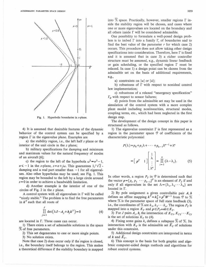
Fig. I. Hyperbolic boundaries in s-plane.

4) lt is assumed that desirable features of the dynamic behavior of the control system can be specified by a region f in the eigenvalue plane. Examples are

a) the stability region, i.e., the left half s plane or the interior of the unit circle in the z plane;

b) military specifications for damping and minimum and maximum values for the natural· frequency of modes of an aircraft [6];

c) the region to the left of the hyperbola C~i=u2 -1,

u < - 1 in the s-plane, s = u + jw. This guarantees 1/ V2 -damping and a real part smaller than - 1 for all eigenval­ues. Also other hyperbolas may be used; see Fig. 1. This region may be bounded to the left by a large circle araund s = 0 in order to achieve a bandwidth Iimitation.

d) Another example is the interior of one of the circles of Fig. 2 in the z plane.

A control system with all eigenvalues in f will be called "nicely stable." The problern is to find the free parameters in k T such that all roots of

J

TI det(Al-Aj+bjkT)=O J-l

are 1ocated in r. Three cases can occur.

(4)

_ 1) There exists a set of admissible solutions in the space X of free parameters.

2) This set degenerates to one or more single points. 3) No solution exists. Note that case 2) does occur only if the.region is closed,

i.e., the boundary itself be1ongs to the region. This makes a theoretical difference if the stability boundary is mapped

1059

into X space. Practically, however, smaller regions r in­side the stability region will be chosen, and cases where one or more eigenvalues are located on the boundary and all others inside r will be considered admissible.

One possibility to formulate a well-posed design prob­lern is to imbed r into a family r, of boundaries and to find the best value of the parameter r for which case 2) occurs. This procedure does not allow taking other design specifications into consideration. Therefore, here r is fixed and it is assumed that in case 3) a richer controller structure must be assumed, e.g., dynamic linear feedback or gain scheduling, or the specified region f must be relaxed. In case 1) a design point can be chosen from the admissible set on the basis of additional requirements, e.g.,

a) constraints on I u I or I u I; b) robustness of r with respect to nonideal control

law implementation; c) robustness of a relaxed "emergency specification"

rE with respect to sensor failures; d) points from the admissible set may be used in the

simulation of the control system with a more complex plant model including nonlinearities, structural modes, coupling terms, etc., which bad been neglected in the first design step.

The development of the design concept in this paper is structured as follows.

1) The eigenvalue constraint r is first represented as a region in the parameter space <5' of coefficients of the characteristic polynomial

In other words, a region Pr in <5' is determined such that the vector p=[p0 PI · · · Pn-dT is an element of Pr if and only if all eigenvalues in the set A= {A.., A2 • ··An} are located in r.

2) By pole assignment a given controllable pair A, b defines an affine mapping kT =kÖ +prw-I from <5' to X where Xis the parameter space of full state feedback (3), i.e., the coordinates of X are ki, k2 • • • kn . The region Pr is mapped into a region Kr andpEPf**kEKr.

3) For J pairs Ap bj the intersection of Kn, Kn · · · KrJ is the set of solutions Kr to ( 4).

4) Fixing some gains k; defines a subspace X of X. Its intersection with Kr is the admissible set Kr of solutions under this constraint.

5) Additional design constraints are interpreted in terms of k and Kr.

6) This concept is the basis for both graphic and alge­braic computer-aided design methods and algorithms for robust control systems.

1060 IEI!I! TRANSAcnONS ON AUTOMATie CONTROL, VOL. AC-25, NO. 6, DI!CI!MBI!R 1980

Parameter space methods have a long tradition, mainly in Russia and Yugoslavia. Siljak [1 , eh. 1, 2] gives a historical review of the work by Vishnegradsky, Neimark, Mitrovic, and himself. In these methods an arbitrary controller structure with free parameter vector k can be assumed. The characteristic polynomial

n

P(A)= ~ P;(k)Ai =0 (6) ;-o

defines a map x ..... '?J> which has to be inverted in order to map boundaries from '?]> to :Je. In this paper the Controller structure is restricted to state feedback (3), and the map '?Jl~:JC is determined directly via pole assignment. The following diagram summarizes the relationships between A, '3>, and X for state feedback.

P(A)-'1T(A-A1 ) kr-k~+prw-•

A <) '3> <) X numerical P(A)=det(AI-A +bkr)

factorization

Apparently it is easier to go in the direction A ..... '?J>~X than in the opposite direction. In other words, it is easier to study the effect of one eigenvalue A; on kT than to study the effect of one gain k; on A.

II. REPRESENTING AN EIGENVALUE REGIONrAS A

CHARAcrnRisnc PoL YNOMIAL CoEFFICIENT REGION

Pr

Let the region r in the A-plane A =V+ jw be bounded and symmetric with respect to the real axis. The boundary

w2 =w2(v) (7)

has intersections vRi• i=l,2:··2N, with the real axis w2(vR;)=0.

Assurne that the eigenvalues are varied continuously until one or more of them cross the boundary (7). This may occur for a real pole at vR, w2(vR)=O, or for a complex pair of poles v ±jw on the boundary (7).

A. Real Root Boundary

Fora real root at A=vR

P(A) = (A -vR) · R(A),

R(A)=r0+ r1A+ · · · +rn_2 An-2 +An- I. (8)

The coefficients P; are linear in the remaining n- I free parameters r0, r 1 • • • rn _2, i.e., the boundary in '3> space is an (n- 1)-dimensional hyperplane. Its equation is

(9)

B. Complex Root Boundary

Fora complex pair A=v±jw on the boundary (7)

P(A) = Q(A)R(A)

Fig. 2. Circular boundaries in z-plane.

Q(A) = (A-v-jw)(A -v+ jw)

=A2 -2vA +v2 + w2( v)

R(A)=ro+r.A+ .. . +rn- 3.\"-3 +>-.n-2.

(10)

The coefficients P; depend nonlinearly on the n- I free parameters v, ro ... rn-3' However, for a fixed V, i.e., one fixed complex pair on the boundary, they are linear and the boundary is an ( n- 2)-dimensional hyperplane. As v varies, this hyperplane moves and forms the complex root boundary. Another way of viewing this same surface is to keep the n- 2 eigenvalues in R( A) fixed and to move the complex pair along the boundary. This generates a one­dimensional curve p( v ). The shape of this curve depends on the boundary w2( v ).

Some boundaries of particular interest are as follows. I) Imaginary axis, stability boundary for A=s.

v=O, Q(A)=A2 +w2,

p linear in w2 for fixed R(A).

2) Parallel to imaginary axis

v=v1, Q(A) =A2 -2v 1A+v~+w2 ,

p linear in w2 for fixed R(A).

3) Conic section, symmetric to the real axis, i.e.,

Some special cases follow.

(11)

c2 < 0, ellipse: of particular interest are circles c2 = -1, constant natural frequency curves in the s-plane, stability Iimit, and other boundaries in the z-plane. See Fig. 2.

c2 =0, parabola, or if also c 1 =0, C0>0, straight line

parallel to real axis. For c0 =c1=c2 =0 real axis, 1.e., boundary between real and complex eigenvalues.

c2 > 0, hyperbola: in particular two straight lines for w2 = c2( v-v0 )

2, c2 > 0, e.g., constant damping lines in the

s-plane. This boundary is frequently combined with a

ACKERMANN: PAllAMETER SPACE DESIGN

a)

11 2

m I V

Po

c)

~c b)

Fig. 3. Real and complex root boundaries partition the q plane ~to five regions. ABC is the stability triangle for second-order discrete-time systems.

parallel to the imaginary axis. Here it is more convenient to use a hyperbola, which guarantees the required damp­ing and minimum negative real part of the eigenvalues. See Fig. 1.

Substituting (11) into Q(A)

Q(A)=A2-2vA+(1 +c2 )v2 +c,v+c0 • (12)

Variable p is quadratic in v for fix.ed R(A). It becomes linear if and only if c2 = -1, i.e., for a circular boundary in A plane. In other words, if the ~ - 2 roots of R( A) are fixed and the remaining two roots of P(A) move as a conjugate pair along any circle in the A-plane with center A on the real axis and radius r, then the corresponding

0

point in 0> space moves along a straight line. lts endpoints correspond to double eigenvalues at the axis intersections AL =A

0 -r and AR =A

0 +r of the circle, i.e., QL(A)=(A­

AL)2 and QR(A)=(A-ARi· The polynomials PL(A)= QL(A)R(A) and PR(A)=QR(A.)R(A) represent the end­points of this straight line segment in the 0> space.

For second- and third-order systems it is possible to visualize regions in 0> space graphically. This is done in the following for the unit circle in the A=z plane, i.e., the stability region of discrete systems in the 0> space is determined.

For n=2 a) Real root boundary for z = l. By (9) the boundary is

the straight line P(l) =po +p1 + 1 =0. b) Real root boundary for z=-1, P(-1)=p

0-p1 +l

=0. c) Complex root boundary v2 + w2 =I, - 1 < v < 1. In

(10) R(A)= 1, P(A)=Q(A)=A2 -2vA+ 1, Po= 1, Pt= -2v, -2<p1 <2.

Fig. 3 shows the three boundaries. At B the two real root boundaries intersect, i.e., P8 (z)=(z-l)(z+ 1), p~ =

~----------

1,

I ' I \ I \ I I I I I I

Pz \ I I \ I I

Po

\ I

\1 I (.. ___ _ __ __ .l._

0

1\ I \ I \ I \ r-j I I I I I I I I

-~ I I

\ I ' I \I __ _ __ ..ll

c

Fig. 4. Stability region for third-order discrete-time systems.

1061

[- 1 0]. Similarly PA( z) = ( z + I?, i.e., ii = (l 2] and Pc(z)=(z-1)2, i.e., p~ =[1 -2). The boundaries a), b), and c) partition the Po -p 1-plane into five regions such that I) both poles are inside the unit circle; II) one left, one inside; 111) one left, one right; IV) one inside, one right; V) complex outside or both left or both right [a distinction between these three cases in region V) would require a further boundary distinguishing real and com­plex roots]. Usually only the stability region I is of inter­est.

For n=3, only the stability region is shown in Fig. 4. Its real root boundaries are the triangles ABC in the plane P( -1)=0 and BCD in the plane P(l)=O. The complex boundary is obtained by (10), P(A)=(A2 -2vA+ 1)(r0 + A). Fora fixed value of r0 it is a straight line from a point on BA(v= -1) to a point on DC (v= 1). Fora fixed value of v it is a straight line from a point on AC (r0 = 1) to a point on BD (r

0 = -1). This second-order surface is a

hyperbolic paraboloid. lt has a saddle point at pr = [0 1 0]. The stability region is uniquely determined by its vertices A, B, C, and D which correspond to the four polynomials with zeros in the set { - I, 1), i.e., ii = (l 3 3], p~=[-1 -1 1], p~=[l -1 -1], and p~=[-1 3 - 3]. lt is seen from Fig. 4 that the tetrahedron ABCD is the convex hull of the stabi1ity region.

Farn and Meditch [2] showed that this property gener­alizes to arbitrary degree n of the characteristic poly­nomial. For an nth-order linear discrete system the con­vex hull of the stability region in 0> space is a polyhedron whose vertices correspond to the n + 1 polynomials with zeros in the set { -1, 1 }.

Let the vertices be ordered such that the vertex vector p1

corresponds to the polynomial P1 =(z-1t- 1(z+ 1)1, i=

0; 1, 2 · · · n. The n + 1 vertices are independent, i.e., the vectorsp1 -p0 , p2 -po· · · Pn -p0 are linearly independent. Therefore, any vector p can be unique1y expressed as

n

(13)

1062 IEEE TRANSACOONS ON AUTOMATIC CONTROL, VOL. AC-25, NO. 6, DECEMBER 1980

with n

(14) ;- o

J-1.; are called "barycentric coordinates" of p [3]. Variable p may be visualized as the center of mass of the polyhedron if a unit mass may be distributed arbitrarily over the n + I vertices. As long as the masses J-1.; arepositive the center of mass is inside the polyhedron. The interior of the poly­hedron is an n-dimensional simplex. lt is characterized by the fact that the barycentric coordinates are nonnegative JJ.; > O, i=O, J .. · n. Equations (13) and (14) may be writ­ten

(15)

where p belongs to the simplex if and only if all elements of

(I6)

are nonnegative (or positive if we consider the open region, which corresponds to the interior of the unit circle in the z-plane without the circle itself). Equation (16) gives the strongest linear necessary conditions for stability of a discrete system.

lt follows from (I2) with c2 =-I that the convex hull property generalizes to arbitrary circles with radius r and center V

0 on the real axis of the eigenvalue plane. This

circle intersects the real axis at vL =vo-r and vR =vo +r. The vertices of the convex hull of the corresponding region in <5' space are determined by the n + I polynomiais with zeros in the set { Vv vR}· This may also be shown by reducing this problern to the previous one via z' = ( z­v

0)jr. lt is, therefore, convenient to specify the eigenvalue

region by one member of the family of nonintersecting circles f, shown in Fig. 2. lts equation is

(v-vo)2+w2 =r2

v0 ( v0 - I) =0.99r( r - I) ,

v0 =0

v0 < 0.5 for r< I (I7)

for r> I.

For r= 0 it is the deadbeat solution with all eigenvalues at z=O. With increasing r, the center v0 of the circles moves to the right until it reaches 0.45 for r=0.5 where it then goes back to zero to produce the unit circle for r= I. If boundaries in the unstable region are needed, con­centric circles with radius r may be used. Circles with radius r in the range 0.3-0.5 approximate the usual loga­rithmic spirals for constant damping augmented by a constraint on I z I· This eigenvalue region corresponds to well-damped transients. The right shift of the circles ex­cludes heavily oscillatory solutions. Faster solutions with r_.o typically require larger control inputs I u I and allow

less robustness with respect to plant parameter variations. The family of circles (17) builds a bridge between the

practical aspect, that most newly designed control systems are digital, and the theoretical aspect, that (I2) is linear in v for circles only.

For continuous-time systems the fami!y of hyperbolas rP of Fig. 1 in the s( = a + jw )-plane may be used. Its equation is

w2 = -p2 +a2 fp2 for a<O

a=-p fora>O.

For large p an extremely fast solution is obtained: p= 1 gives the I/ v'2 damping Iine as asymptotes; for p~O it goes to the imaginary axis. Negative p represent parallels to the imaginary axis in the right half plane.

111. MAPPING FROM <?J' SPACE TO :JCSPACE

(POLE ASSIGNMENT)

A controllable pair (A, b) defines via pole assignment a mapping from <5' to X space. This mapping is affine, i.e., it consists of a translation and a nonsingular linear mapping

(18)

The foundation of this mapping is Theorem I. Theorem 1 (Pole Assignment): Given a polynomial P(A)

=po +piA+' '' +Pn- IAn-I +An=[ PT l]A, A=[l A · · · An f , an n X n matrix A, and an n X 1 vector b such that det R~ O, R=[b, Ab··· An- 1b]. The unique solution to

det(A/-A+be)=[ PT I]A. (19)

lS

(20)

where eT is the last row of R - 1•

Proof' Existence and uniqueness of the solution were shown by Rissanen [4] by transformation to control canonical form. The solution in form of (20) is derived as follows.

Let F=A -bk' and expand powersofF in terms of the form A;bkTFi.

F 0 =A0 =1

F=A-bkT

F 2 =A2 -AbkT -bkTF

Fn=An-An - IbkT -An- 2bkTF

- ... - bkTFn-I

(I)

(2)

(3)

(n+ I).

Multiply the first equation by p0

, the second by Pt> etc.,

ACKI!RMANN: PARAMETER SPACE DESION

the (n+ l)st row by one, and add the equations

P(F)-P(A):_ [ h, Ab· .. A"-'b ]UT l By Cayley-Hamilton P(F)=O. Then

[.'r ]~r'P(A), R~[b,Ab· · ·A"- 'h]

kr must satisfy the last row, i.e.,

Explicitly

kT= eT[Po1+piA+· ·· +Pn-IAn-I+An]

(21)

Q.E.D. (23)

The form (22) of the result was derived in [5]. Equation (23) may be rewritten in the form of (18) with

(24)

Note that W is the matrix that transforms A, b to the control canonical form

(25)

This is a more popular way of doing pole assignment. It was shown in [5] that the columns W; of W=[w1 • • • wn] can be determined recursively by Leverrier's algorithm:

B0 =1

This describes the mapping from 9C to qp as

pr =(kr -k'{;)W=krW+ar,

1063

(27)

Equations (26) and (27) also provide an alternative way to determine the pole placement matrix E in (20) as

E= [ w-l ]

-arw-I · (28)

In numerica1 calculations of E with !arge n the accuracy of the vectors erA;, i=l,2,-· ·,n must be checked. One test is to letp0 =p 1 • • • =Pn - l =0. Then kT =eTAn. Evaluate det('A/ -A +beTAn)=fto+fti'A + · · · +ftn-1)\n-l +An. Theftj should ideally be zero. Their magnitude is a measure for the error in eTAn. Another convenient test follows from the definition of eT:

i=O, 1, · · ·, n - 2 i=n-1.

(29)

It is easily seen that this property is also preserved for the closed loop

eT(A -bkr)ib= { 01

i=O, 1,- · · n-2 (30) i=n-l.

This relation also implies that the vectors er, erA · · · eTAn-t areinvariant under state feedback (A, b)~(A ­bkr, b). They are a complete set of invariants of this feedback equivalence class since they uniquely determine a realization in control canonical form with undeterrnined characteristic polynomial.

The (n+ l)Xn pole placement matrix Eisa convenient representation of a controllable pair A, b, i.e. , the element k=O of the feedback equivalence dass. The general ele­ment may be characterized as

eTAn-1

eTAn-kT

(31)

The mapping of a point p in qp to a point k in 9C via k T = [ pr I] E requires only n 2 m ultiplications and n2

additions. This compares favorably with mapping a trial

an- t = -tr A~

an- 2 = - -i-tr ABI

B1 =A~+an_ 11

~ =AB1 +an_21

wn =Bob

"'n-1 =B,b

-1 =-trABn- t

n 0

(26)

=ABn-l +a01 (check).

1064 IEEE TRANSAcnONS ON AliTOMATIC CONTROL, VOL. AC-25, NO. 6, DI!CI!MBI!R 1980

design point from the parameter space of quadratic criteria via the Riccati equation into 9C space. This is an ad­vantage for computer-aided design methods in which many trial design points have to be mapped and displayed graphically.

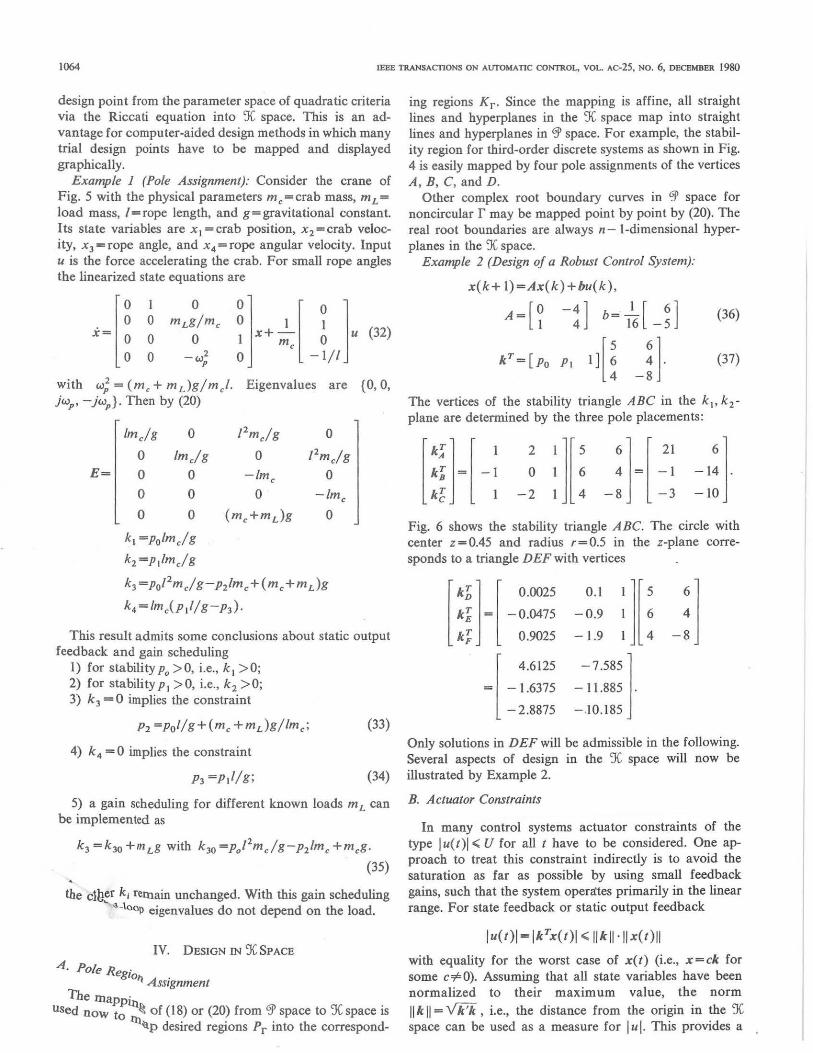
Example 1 (Pole Assignment): Consider the crane of Fig. 5 with the physical parameters mc=crab mass, mL = Ioad mass, /=rope length, and g=gravitational constant. Its state variables are x 1 =er ab position, x 2 = crab veloc­ity, x3 = rope angle, and x 4 = rope angular velocity. Input u is the force accelerating the crab. For small rope angles the linearized state equations are

x~[~ 1 0 0

x+ ~< [ ! 1 u (32) 0 mLgfmc 0 0 0 1

0 -w2 0 -1/1 p

with w; = (m c + mL)gjmJ Eigenvalues are {0, 0, jwP, -jwp}· Then by (20)

/mcfg 0 [2mjg 0

0 lmcfg 0 [2mcfg

E= 0 0 -lmc 0

0 0 0 -lmc

0 0 (mc+mL)g 0

kl =pofmcfg

k2=pllmcfg

k3 =pol2mcfg-p2/mc +(mc + mL)g

k 4 =lmc(p11/g-p3).

This result admits some conclusions about static output feedback and gain scheduling

1) for stability Po> 0, i.e., k 1 > 0; 2) for stability p 1 > 0, i.e., k 2 >0; 3) k 3 = 0 implies the constraint

P 2 =p0 1/g+(mc +mL)gjlmc; (33)

ing regions Kr. Since the mapping is affine, all straight lines and hyperplanes in the 9C space map into straight lines and hyperplanes in 0' space. For example, the stabi1-ity region for third-order discrete systems as shown in Fig. 4 is easily mapped by four pole assignments of the vertices A, B, C, and D.

Other complex root boundary curves in 0' space for noncircular r may be mapped point by point by (20). The real root boundaries are always n-I-dimensional hyper­planes in the :Je space.

Examp/e 2 (Design of a Robust Control System):

x(k+ 1)=Ax(k)+bu(k),

A=[~ -:J b=1~[-~] (36)

kr =[Po P1 I)[~ ~] (37) -8

The vertices of the stability triangle ABC in the k., k 2 -

plane are determined by the three pole placements:

[ :~]=[ _; ~ :j[~ :j=[ ~~ -l:j. k~ 1 -2 1 4 -8 -3 - 10

Fig. 6 shows the stability triangle ABC. The circle with center z = 0.45 and radius r = 0.5 in the z-plane corre­sponds to a triangle DEF with vertices

[ k~l [ 0.0025 k~ = -0.0475

k~ 0.9025

[

4.6125

= -1.6375

-2.8875

0.1

-0.9

-1.9 :][! _;]

-7.585] -11.885 .

-10.185

4) k 4 = 0 implies the constraint

PJ =p1ljg;

Only solutions in DEF will be admissible in the following. Severa1 aspects of design in the :JC space will now be

(34) illustrated by Example 2.

5) a gain scheduling for different known Ioads mL can be implemented as

kJ =k30 +mLg with kJo =p)2mcfg-p2/mc +mcg.

(35)

the clber ki rernain unchanged. With this gain scheduling " -\oop eigenvalues do not depend on the Ioad.

IV. DESIGN IN :Je SPACE

A. Pole Reg; 0 11 A.ssignment

The rnappin_ used now to ~ of (18) or (20) from 0' space to 9C space is

lll~p desired regions Pr into the correspond-

B. Actuator Constraints

In many control systems actuator constraints of the type I u(t)i < U for all t have to be considered. One ap­proach to treat this constraint indirectly is to avoid the saturation as far as possible by using small feedback gains, such that the system opera:tes primarily in the linear range. For state feedback or static output feedback

iu(t)i =ikrx(t)i < llkll·llx(t)ll

with equality for the worst case of x(t) (i.e., x=ck for some c'foO). Assuming that all state variables have been normalized to their maximum value, the norm II k II = Vk'k , i.e., the distance from the origin in the :Je space can be used as a measure for iui. This provides a

ACKERMANN: PARAMETER SPACE DESIGN

crab mass mc

Ioad mass ml

Fig. S. A crane or loading bridge.

Fig. 6. Design in X plane for a second-order discrete-time system.

criterion for the selection of a gain from the adm.issible set: choose the point closest to the origin. In the example of Fig. 6 this is G with kb=[2.8-8.2]. Equation (27) is here

6 )·_!_=[4 -4]. - 5 16

(38)

Thus, kb maps into Pb= [0.225 - 0.388] with eigenvalues z1,2 = 0.194 ±j0.433. This is the most gentle way tobring the double eigenvalue atz= 2 into f 0.5 . Note that the gain reduction margin of G is 21 percent. The maximum gain reduction margin would be achieved at E where it is 26 percent.

C. Robustness with Respect to Measurement Noise and Quantization Effects in the Controller

The feedback control law may be implemented ap­proximately in a short wordlength microprocessor as

where Ll2 u is the output quantization error, which may be neglected here as weil as the product of small terms LlkT·Llx. Then

(40)

is the error resulting from measurement noise and input quantization in Llx and quantization LlkT of the feedback gains. The first term kTLlx is kept small by minimizing II k II as illustrated in Section IV -B. The second term re­quires that some distance from the boundary must be kept as safety margin.

In the example of Fig. 6 Iet Lle = [ ± 0.3 ± 0.3]. This margin is maintained at the center of the 0.6 X 0.6 square inside DEF (indicated by omitted shading) which is moved as close as possible to G. lt results in

kT = [2 -8.9] ,

PT= [0.1625 -0.46875],

z 1.2 = 0.234 ±)0 .328.

D. Robustness with Respect to Sensor Failures

(41)

Sensor failures are assumed to occur in the form that the sensor output is no Ionger correlated with the. mea­sured variable. As far as the characteristic equation is concemed, this is equivalent to having a sensor output zero. There may be a bias or other noise term introduced by the failed sensor. This noise term can be considered as an extemal input. This may require that the failure is detected and the failed sensor is removed from the control system. Then the controllaw may also be changed. How­ever, for this latter decision there should be sufficient time to come to a reliable decision without false alanns. This requires that after the failure the system at least remains stable with some stability margin. In other applications it may suffice to be able to continue the mission after a sensor failure without removal of the failed sensor, e.g., to drive an automobile safely to a service station to get a broken sensor replaced, such that optimal fuel economy, emission control, acceleration, etc., is regained.

It is not reasonable to require the poles to remain in the same region r as in the unfailed situation; thus, a relaxed "emergency region .. rE is introduced. Here is the robust­ness problem: consider M failures of a sensor or combina­tions of sensors leading to the crippled feedback vectors k ~, m = I, 2, · · · , M in which the appropriate elements of kT are replaced by zero. Find kT such that all zeros of

M

fl det(.H-A +bk~)=O (42) m - 1

lie in the emergency region rE in the A.-plane. The emer­gency specification is robust with respect to a failure of sensor i if and only if in the 9C space the projection of kT into the subspace k; =0 is in the emergency region KrE·

Fig. 7 shows an example of emergency and nominal regions in the k 1 -k2 -plane. If we choose kT at point 1, then the projection on the k 2 axis is inside the emergency boundary, i.e., f E is robust with respect tO a failure Of sensor I. It is, however, not robust with respect to a failure of sensor 2, since the projection on the k 1 axis is outside the emergency region. Points in the shaded region

1066 IEEE TRANSACfiONS ON AUTOMATIC CONTROL, VOL. AC-25, NO. 6, DECEMBER 1980

Fig. 7. Robustness with respect to sensor failures.

are robust with respect to failure of either sensor. For no krrE is robust with respect to failures of sensors I and 2, since the origin k 1 =k2 =0 lies outside the emergency region. Point 3 also meets the nominal specification and is a good candidate for further study and simulation. Since the nominal boundary intersects the k2 ax.is, an alternative to the robust solution 3 is to eliminate the x 1 sensor and to multiplex the x2 sensor. This would maintain the nominal specifications under a failure of one of the x2 sensors. However, it requires failure detection with at least three x 2 sensors.

In the example of Fig. 6 it turns out that for the previously selected solution (41), stability is robust with respect to failure of sensor I since it is in the shaded region around the k2 -ax.is. However, no reasonable tradeoff can be made to achieve robustness with respect to failure of sensor 2, i.e., to go to the right shaded region. In other words, the sensor for x2 is the more important one. If it is not reliable and the mission is critical, then this sensor must be multiplexed.

Independent of the chosen controller structure, a neces­sary condition for robustness of r E with respect to a failure of one or more sensors is that the eigenvalues of A outside rE remain observable after a failure. It is an open question whether this condition is also sufficient, i.e., whether there exists a Controller structure and constant parameters in it such that robustness of rE with respect to all failure combinations which leave the eigenvalues out­side rE Observable is achieved.

E. Robustness with Respect to Large Plant Parameter Variations

Assurne that the plant model

.i=A( 9)x+b( 9)u (43)

is given for several typical values of the physical parame­ter vector 9, i.e., Aj=A(9), bj=b(O),J= 1,2· · · J. A fixed­state feedback is sought, such that all zeros of

(44)

are located in a specified region r in the ;\-plane, i.e., p is located in the corresponding region Pr in the GJ space.

Each pair Aj, bj Ieads to a different matrix E. in (20). Pr is mapped by kT =[PT I]Ej into J different ~egions K . in the 9C space. The set of solutions to the problern (44), J it exists, is the intersection of these J regions in the 9C space. If no intersection for allj=l,2 .. ·J exists, then it can be tested whether at least a group of plant models can be nicely stabilized with one gain and it may be necessary to switch to a different gain for a different group of plant models.

As an example Iet n = 2, J = 2, and r be circular. The solution is the intersection of two triangles. This intersec­tion may be empty, a triangle, a quadrangle, a pentagon, or a hexagon. With an increasing nurober J of plant models, many more cases of polygons have to be dis­tinguished. It is not advisable to solve this problern numerically, i.e., to calculate the vertices of the inter­secting polygon, since the designer is not interested in the number of vertices. For him it is important to know whether the intersection is nonempty and what its ap­proximate size and extension is. In the interaction be­tween a designer and a computer-aided design system this task of finding the intersection on a display should be assigned to the designer.

Now Iet n=3, J=2, and r be circular. The nice stability regions Krj are affine to the region of Fig. 4. For each Operating pointj they are deterrnined by four pole place­ments of the vertices A, B, C, and D. The complex boundary is then constructed by dividing each edge into equal segments and connecting the corresponding points by straight lines.

Here we can draw an important conclusion from the possible intersections of two bodies of the shape of Fig. 4: the admissible set of solutions may be disconnected. This is seen if we visualize a second body of the same shape upside down such that two intersections of the tips near A and D occur. In numerical methods a systematic search may be necessary in order to find all parts of the admissi­ble set. Here it is helpful to Iimit this search to the intersection of the convex hulls, in the example the two tetrahedra. If this intersection is empty, then no robust solution exists. If it is nonempty, then this intersecting polyhedron defines the search space, where at least the necessary condition for a robust solution is satisfied.

For arbitrary n a point k in the 9C space can be tested algebraically as to whether it belongs to the simplex of stability or nice stability. This is formulated as Theorem 2.

Theorem 2: A necessary condition for kr to stabilize x(k+ I)=(A -bkr)x(k) isthat all elements of

-I

kÖ kT

p_T = [kT I) I (45)

kT n

ACKERMANN: PARAMETER SPACB DESIGN

are positive, where k'{ assigns the characteristic poly­nomial P(z)=(z-1)"-;(z+ 1);,_ i=O, 1,2· · · n.

Proof' Substitute (I5) into (20):

E=p7

This is augmented by (I4):

(46)

and inverted to give (45). Q.E.D. The generalization to other circles is obvious. Different

plant models result in different ~ and thus different vertices k~· · · k~ of the simplex and different barycentric coordinates p.) in (45). kr is in the intersection of sim­plexes if all these Coordinates are positive. This is a necessary condition for a robust feedback.

For different values ~ of the physica1 parameter vector, different regions IJ in the ll. plane may be given and the intersections of the corresponding % space regions must be found. Such parameter-dependent pole regions are given in military specifications for aircraft modes [6]. This reflects the fact that the pilot, for example, expects the aircraft to react more slowly in landing approach than in terrain following at high speeds. A general recommenda­tion for the design of robust control systems with actuator constraints is to try not to make a slow plant fast or a fast plant slow by feedback. This is an essential difference to all high-gain design concepts which locally reduce the sensitivity of a nominal trajectory x(t) or deviation from a reference model response under plant parameter varia­tions. Pole region assignment in connection with soft feedback, i.e., minimum II k 11, offers more flexibility to also accommodate !arge parameter variations with medium control magnitudes. This point is further illustrated by the crane example (32). The gain scheduling control of (35) keeps the eigenvalues constant in spite of Ioad variations. But even if m L is known, this control is undesirable because in view of constraints on the available force I u 1, positioning of the empty hook should be performed faster than positioning of the maximum Ioad. It is important to also keep this point in mind in multiinput problems where this aspect may be obscured by the !arge number of remaining free parameters after the poles have been as­signed. Even the best choice of these parameters cannot compensate for speeding up the modes too much by pole placement.

1067

V. PARTIAL GAIN ASSIGNMENT, OUTPUT FEEDBACK

The concept of graphical % space design of robust control systems was introduced for a second-order system with only two free feedback gains k1 and k 2• Also three­dimensional regions and their intersections can be made visible by computer graphic methods which permit anima­tion, rotation, change of viewing direction and distance, multicolor, and stereoscopic displays.

A fourth dimension of the parameter space can be translated into time, but here we would reach the Iimits of our imagination. The design can then be performed in iterative steps, such that in each step only the influence of two or three parameters is studied, while all other gains are fixed. Also other design constraints, like output feed­back or sensor failure cases, can require that some gains in kT are fixed in advance. This means that we are looking for a solution in a subspace of %. Such a solution may not exist; take for example Fig. 6 and fix k 1 tobe bigger than k 1(A). Then there does not exist a stabilizing k 2 • The set of admissible solutions may also become disconnected, even if it is connected in the % space; take, for example, a stability region such as that in Fig. 4, map it into the % space, and fix one k; suchthat the plane k; =c intersects the two tips of the stability region.

Examp/e 3 (Disconnected Stability Regions in a Subspace of %):

x(k+ I)= [ ~ 0.6

~ ~ ]x(k)+[~ ] u(k). (47) -2 2.1 I

The system is open-loop unstable (eigenvalues z1 =0.5, z 2, 3 =0.8±jY0.56 ). Fix k 2 =0 (output feedback) and find the set of stabiiizing gains in the k 1 - k 3 -plane. The real root boundaries are the straight lines

for z = I

for z= - 1

k3+ = -kl - 0.3

k3 _ = -kl +5.7

and the complex root boundary is the hyperbola

Fig. 8 shows the three boundaries and the two discon­nected stabilizing regions. lts vertices are

kl k3 E -0.4 0.1 F 0.1 -0.4 G 1.1 4.6 H 1.6 4.1.

Nonconvex and disconnected solution sets such as in this example Iead to difficulties in numerical algorithms. Sirisena and Choi [7] formulate the problern of placing poles in a specified region by output feedback as minimi­zation of a function J which becomes zero if a solution is found. Their conclusion from computa tional experience is, " If, however, a local (nonzero) minimum of J is

""''

1068 IEEE TRANSAcnONS ON AUTOMATIC CONTROL, VOL. AC-25, NO. 6, DECEMBER 1980

reached, the algorithm s·hould be restarted with a different initial value of the feedback matrix. Repeated failure to reduce J to zero would indicate the absence of a solution."

An alternative is a search in the region where the necessary condition to be in the simplex is satisfied. In Fig. 8 this is the quadrangle EFHG; in general, it ·is the polyhedral cross section of the subspace given by the fixed k; with the simplex. If no such cross section exists, it can be concluded that no solution exists. The example in­dicates that points near the real root boundaries are prornising candidates.

The effect of fixed gains on the characteristic poly­nornial can be seen by (20):

kT- [k k - I 2

E= [ 1J1 1J2

kn]=[ PT I]E,

1Jn].

Fixing k; implies a linear relationship

(48)

between the coefficients of the characteristic polynornial. If g gains are fixed it is convenient to factor out a gth-order polynomial R(A.) from P(A.)=R(A.)Q(A.) such that assigning a remainder polynornial Q(A) together with the g gains deterrnines R(A.) and the n-g free gains of kr. The coefficients of the product polynornial may be written

[ PT 1) = [Po · ·. Pn - I I)

= [r. · · · r I] 0 g-1

0

where S is a gX(n+ I) matrix and tT a I X(n+ I) vector. Let kJ be the fixed gains, which for convenience are chosen to be the last g gains in kr. Then

kT=[k~ krJ=[ PT l][Ea Eb]

=[rr l ][ ~][Ea Eb]

kJ = rTSEb + tTEb

which can be solved for

(50)

if the gXg matrix SEb is invertible. Note that this condi­tion does not depend on the values of kJ; thus, this is the sameproblern as in output feedback kJ =0 where certain pole locations cannot be achieved. Variable k~ is de­termined by

Assigning the n-g eigenvalues of Q( A) deterrnines S. The remaining g eigenvalues can be deterrnined by factoring the residual polynornial R(A.) with coefficients given by (50).

Example 4 (Fixed Feedback Gains): For the crane of Example 2let k 1 and k 4 be fixed, i.e., k~=[k2 k 3 ],kJ= [kl k4]:

0 /2mc/g lmc/g 0

lmcfg 0 0 /2mcfg E= a 0 -/mc Eb= 0 0

0 0 0 -lmc

0 (mc+mL)g 0 0

Then by (50)

rT=[ro ri]

=[kl k + I ]·[qolmc/g 4 ql mc O

Theinverse exists if q0 =l=g/l and q0 =/=0. Then

klg qlmc - klqifqo+k4/l r0= -- r1 = (52)

q0 /mc' mc(q0 /jg - l)

and with (51)

0 0

0 (49)

(53)

k 1 will be fixed by the following consideration. Assurne a force limitation I u(t)l < U for all t for a typical operation of the crane, i.e., a displacement of a Ioad at rest, x(O) = [L 0 0 Of, L>O (e.g., length of a loading bridge) to a final position x(tE)= [O 0 0 Of. Typical responses of suf­ficiently stabilized cranes show an initial peak u(O) of the force as the maximum value of lu(t)l. A simple approach to avoid saturation is, therefore, to meet a necessary condition by fixing I u(O)I = U and checking the conditions for u(O)/u(O)<O. Then lu(t)l for t>O may be checked in a simulation. Here

u(O)= -kTx(O)= -k1L

ACKERMANN: PARAMETER SPACE DESIGN

Fig. 8. Disconnected stability region in k 1 - k3 subspace.

u(O)= -kT(A -bkT)x(O)

=Lk1(k 2 -k4ll)lmc=Lk 1p 3 • (54)

Thus, u(O) I u(O) = - I I p3 < 0 for all stabilizing feedbacks and I u(O)I = U results in k 1 = U I L.

It is desirable to avoid the difficult measurement of the rope angular velocity x 4 • Thus, k 4 = 0 is chosen. Then by (52)

(55)

Variables ro and r1 are the coefficients of the residual polynomial which is obtained after qo and q1 have also been fixed. Necessary and sufficient conditions for stabil­ity are q0 > 0, q1 > 0, ro>O, r1 > 0. With (53)

For given values of mc, mL, /, g, U, and L we can now use (52) to map points on a boundary of r in the eigen­vatue plane, i.e., qo- q1 pairs, into the k2 - k3-plane. lf one

A 4233 B 2367 c 2769

-84292 -35012 -22056

1069

TABLEI

Eigenvalues

s1, 2 - -0.25, s3•4 = -1.867±j2.125 s1, 2 = -0.275±j0.231, s3 ,4 ~ -0.908±jl.746 s1 = -0.25, s2 = - 1.337, s3, 4 = -0.591 ±jl.071

of the resulting regions corresponds to the case that all eigenvalues are inside r, then this is the admissible set of solutions. Several such sets may be plotted, e.g., for differ­ent Ioad masses m L or rope lengths I in order to find a robust solution in the intersection. In order to illustrate this, m L is assumed unknown and numerical values for the other parameters are given as mc= 1000 kg, /= 10 m, g= 10 mls2

, U=5000 N, and L= 10m. Example 1 showed that only k 3 =k30 =mLg depends on

the Ioad mass mL' k 30 =k3-IO mL is determined first. For k 1=UIL=500 and k 4 =0 find the region in the k 2 -k30-

plane for which all eigenvalues are left of the hyperbola

(57)

in the s-plane. Then for the complex root boundary from (10)

(58)

and by (55) and (56)

The nice stability region will be constructed in the k 2 -k30-plane. The complex root boundary kio), k 30(o) is obtained by substituting values o< -0.25 into (58) and q

0 and q1 into (60) and (61). The real root boundary at

aR = -0.25 follows from (8) with k 1 = 500, k 4 = 0 as the straight line

k 3 R =k30R + IOmL, k 30R =95625-42.5 K2 • (62)

Both boundaries are shown in Fig. 9. Fora= -0.25 the complex root boundary starts at point A. With increasing a it goes through point B and for o~- 0.5, i.e., q

0 ~ 1 to

infinity. In general, this singularity occurs at q0

= gl /. For a < - 0.5 the complex root boundary retums from the opposite side to intersect the real root boundary at C and itself at B.

Note that the characteristic polynomial is obtained by (58) and (59) in factorized form. Thus, the determination of the eigenvalues is easy. They are given together with the k2 and k 30 coordinates in Table I.

At A the real and complex root boundaries intersect, i.e., there is a double pole at s 1•2 = -0.25. At B the

1070 lEI!!! TRANSACTIONS ON AlTTOMATIC CON'ffiOL, VOL. AC-25, NO. 6, DI!CI!MBBR 1980

Fig. 9. Nice stability region for crane with k 1 ... 500, k 4 - 0.

complex boundary intersects itself. Here we have two complex pairs of eigenvalues crossing the boundary simultaneously. At C a real root at s= -0.25 crosses simultaneously with the complex pair s3,4 • The shaded region with vertices A, B, and C corresponds to eigenval­ues to the left of the hyperbola in s plane.

It is easy now to find the fixed gain Controller which accommodates the largest Ioad variation.

The Ioad mass enters only into k3 = k 30 + 10 mL. In Fig. 9 the origin of the k 3 -axis is identical to k 30 = 0 for m L = 0. With increasing Ioad mass the shape of the region of nice stability is unchanged, but it is moved upwards by 10 m L in the k 2 - k 3 -plane, or equivalently the origin of the k 3 -axis is moved downwards by 10 mL in the k 2 - k 30 -

plane. Thus, for Ioad variations of cranes it is not neces­sary to plot the shifted diagrams in order to find the intersection. The largest Ioad variation can be accommod­ated at the largest extension of the nice stability region in k 3 direction. This is between C and D. D has the coordi­nates k 2 =2769, k 30 = - 45503 and corresponds to the eigenvalues s1,2 = -0.267 ±}0.680 and s3,4 = 1.118 ±}1.872. Thus, k 2 is chosen as 2769. This results in an admissible Ioad variation mL =(- 22056+45503)/10':"2344.7~2345 kg. Assurne that the weight of the empty hook is 50 kg, then k 3 = - 21556 puts the eigenvalues for mL =50 kg at s1 = - 0.25, s2 = - 1.337, s3, 4 = -0.591 ±}1.071 where s1

and s3,4 are on the boundary r. For m L =2395 kg the eigenvalues are at s1,2 = -0.267 ±}0.680 and s3,4 = 1.118 ± }1.872 where s1, 2 is on the boundary. In summary, the solution

kT = [500 2769 -21556 0] (63)

gives the following properties of the control system. 1) Initialpeak in the force u limited to 500L where L is

the required Ioad displacement. 2) No measurement or estimation of the rope angular

velocity x 4 is required. 3) Under the constraints 1) and 2) maximum possible

Ioad variation. The eigenvalues are left of w2 =(2a)2 -1j22

if and only if 50 kg < m L < 2395 kg. Now assume that the crane is designed for a maximum

Ioad of 3500 kg, i.e., a gain scheduling is necessary. The second Ioad range may be chosen as 1155 kg < mL <3500 kg, and k 3= -10506. Then for 50 kg<mL < ll55 kg, k 3 = -21556 must be used and for 2395 kg < mL <3500 kg, k 3 = -10506. For the overlapping range 1155 kg<mL < 2395 kg either gain is good, such that the crane operator can switch between high and 1ow Ioad based on bis very crude Ioad estimate which may be ± 35 percent wrong. This wide overlap provides robustness of the gain schedul­ing scheme.

If the rope length of the crane is varied, the shape of the nice stability region in Fig. 6 changes and an intersection of various regions must be found.

All calculations were done by pocket calculator. The example shows that realistic problems of robust control system design can already be solved with this new method. Another application example was given by Franklin [8]. He designed a robust stabilization for the short period longitudinal mode of an F 4-E aircraft with canards. Uncontrolled, it is unstable in subsonic flight and unsuffi­ciently damped in supersonic flight. Including the actua­tor the model is third-order with two Outputs (accelerome­ter and gyro). For different altitudes and Mach numbers the eigenvalues were p1aced simultaneously in the regions given by military specifications. Also the short period mode bad to remain separated from other modes and the bandwidth was limited in order to avoid the structural vibration frequency range.

Further design examp1es for a dc motor control and a sampled data control of the crane were given in [9].

VI. MULTIINPUT AND DYNAMIC OUTPUT FEEDBACK

PROBLEMS

Forasystem withp inputs, u=[u1 • • • uPf,

.i=Ax+Bu. (64)

The feedback matrix u = -Kr x has p x n free parameters, which define a parameter space % of this dimension.

In the single-input case it was convenient to study the shape of parameter regions in princip1e in a canonical parameter space of the same dimension as %. The particu­lar plant then determined an affine mapping of this region into % space. In the same spirit it is possible to define a p X n-dimensional canonica1 parameter space <3'c [10]. Its coordinates are elements of a p x n matrix pr, the gener­alization of pr in (20). Also E in this equation has a generalization to the multiinput case and the result is a mapping from <3'c to % which is basically of the form

KT =M[PTJ]E

where M is a nonsingular triangular matrix determined by A, B. The characteristic polynomial is then the determi-

ACKERMANN: PARAMETER SPACE DESIGN

nant of a characteristic polynomial matrix with coeffi­cients given by PT. More details are given in (9] and [10]. The dynamic output feedback problern can also be formulated as a multünput problern for an augmented system.

If the parameter space methods show that for a given - Controller structure no solution exists, then one of the

possibilities is to assume a richer controller structure, dynamic output feedback of order m. The plant is aug­mented by m controller states in xc:

and a state feedback

{67)

with m controller inputs in uc is determined, which nicely stabilizes the system (66). The controller M, N, L with n inputs and p outputs may be written in a canonical basis, such that the feedback matrix in (67) contains pn + mn + mp design parameters ((p+m)X(n+m) coefficients in (67) of which m2 are normalized by the choice of an mXm transformation matrix].

For A in sensor coordinates and output feedback the columns of K and M corresponding to missing sensors are zero, and thus the nurober of free parameters is reduced by p + m for each nonmeasured state or failed sensor. Thus, for q measurements the controller has (p+m)q+mp free design parameters. An actuator failure changes n + m coefficients in a row of K and L to zero.

Although basically the generalization of parameter­space methods to multiinput dynamic output feedback problems is possible, the apparent difficulty is owing to the !arge nurober of design parameters. In practical design a more pragmatic way of finding feedback dynamics is more promising. An example was given in the already mentioned design of an aircraft control system [8]. As a result of the first design step robustness with respect to !arge plant parameter variations was achieved and it was shown that, with static output feedback, it is impossible to make the emergency specifications ( damping 0.15 and minimum value for the natural frequency) robust with respect to a failure of the gyro or the accelerometer. Dynamic feedback was designed in the form of two filters connected to the gyro and accelerometer outputs, which provided a second independent signal for the case of failure of one sensor. This defined a four-dimensional parameter space of the feedback gains of the two sensors and their filters.

Finally a solution with two paralleled gyros and one accelerometer was found, which meets the nominal speci­fications for the unfailed system and after a failure of any single sensor, and meets the emergency specifications after failure of any two sensors, where these properties pertain to four very different flight conditions.

1071

VII. CONCLUSIONS

Problems which are usually approached by adaptive control and redundant components with failure detection may also have a fixed gain robust solution. In many cases such a simple robust Controller will be sufficient, as was shown for examples of a crane and an aircraft. Also, if adaptive control and failure detection is used in order to improve the performance, it is helpful to have sufficient time for reliable and accurate identification, adaptation, and failure detection without false alarms. This time can be provided by a robust stabilization system which takes care that immediately after a component failure or sudden !arge parameter change nothing very bad happens. In other words, the adaptation and failure detection is no Ionger vital for stabilization.

Essential for the design of robust controllers are that only physically reasonable requirements are made, which Iead to small feedback gains and control inputs. When the plant is slow it remains slow; when it is fast it remains fast. After component failures, only reduced performance given by emergency specifications can be achieved.

This becomes possible if the pole assignment require­ment is relaxed to a pole region assignment. It was shown how such a pole region is represented as a region in the parameter space q> of coefficients of the characteristic polynomial, and how pole placement defines an affine mapping from the q> space to the parameter space X of state feedback gains. The possibilities of the X space design are illustrated, in particular, actuator constraints and robustness with respect to measurement noise, quanti­zation effects in the controller, sensor failures, and !arge plant parameter variations in known directions.

In summary, 1) X space design in iterative steps is readily applicable

to systems with output feedback. In each design step all feedback gains except two are fixed and the influence of the remaining two gains on the pole location is easily exhibited graphically. This is a practical complement to the root locus method, which shows the influence of only one gain on the eigenvalue location. Also, !arge plant parameter variations in several directions can easily be tackled.

2) Computer graphics will make it possible to Iook at the influence of three gains at a time.

3) Algebraic conditions for arbitrary system order and circular pole regions are available. This is of particular interest for digital control. However, algorithms for the design of robust control systems based on these algebraic conditions are not yet developed.

4) For the multiinput case the formalism is available. lt is, however, not yet fully understood.

Further open research problems are the design for robustness with respect to actuator failures, and a combi­nation of parameter space methods with the Popov method for absolute stability in order to achieve robustness with respect to actuator nonlinearities of a sector type [I].

1072 IEEE TRANSACllONS ON AUTOMATIC CONTROL, VOL. AC-25, NO. 6, DECEMBER 1980

REFERENCES

[I] D. D. Siljak, Nonlinear Systems, The Parameter Analysis and De­sign. New York: Wiley, 1969.

[2] A. T. Farn and J. S. Med.itch, "A canonical parameter space for linear system design," IEEE Trans. Automat. Contr., vol. AC-23, pp. 454-458, June 1978.

[3] W. Franz, "Topologie," /. Allgemeine Topologie, Sammlung Göschen, Berlin, 1965.

[4] J. R.issanen, "Control system synthesis by analogue computer based on the generalized linear feedback concept," in Proc. lnt. Seminar on Analog Computation Applied to the Study of Chemical Processes. Brussels, Belgium: Presses Academiques Europeennes, Nov. 1960.

[5] J. Ackermann, . Abtastregelung (Samp/ed-Data Control). Berlin: Springer, 1972.

[6] · "Flying qualities of piloted airplanes," MIL-F-8785B(ASG), Aug. 7, 1969.

[7] H. R. Sirisena and S. S. Choi, "Pole placement in prescribed regions of the complex plane using output feedback," IEEE Trans. Automat. Contr., vol. AC-20, pp. 810-812, 1975.

[8] S. N. Fran.klin, "Design of a robust flight control system," M. S. thesis, Univ. Illinois, Urbana, 1979.

[9] J. Ackermann, "A robust control system design," in Proc. Joint Automat. Conlr. Conj., Denver, CO, June 1979, pp. 877-883.

[10] "On the synthesis of linear control systems with specified char­acteristics," Automatica, voi. 13, pp. 89-94, 1977.

Juergen Ackermann was bom in Bochum, Germany, on October 5, 1936. He received the M.S. degree in e1ectrical engiDeering from the University of Califomia, Berke1ey, in 1964, the Dr.-Ing. degree from the Technische Hochsch­ule Darmstadt in 1967, and the "Habilitation" from Technische Universitaet Muenchen in 1974.

Since 1962 he has been with the Deutsche Forschungs-und Versuchsanstalt fuer Luft-und Raumfahrt, and since 1974 he has been Director

of the Institut fuer Dynamik der Flugsysteme. In 1978-1979 he was Visiting Professor at the University of Illinois. He is author of the book Abtastregelung (Berlin: Springer), Associate Editor of Automatica, and recipient of the VDE award for contributions in control engineering. His current research interests are in design of robust control systems.