on the robust nonlinear curve fitting - ism.ac.jpfukumizu/coopmathws2014/akaho_coopmathws... ·...

. . . . . .

.

......On the robust nonlinear curve fitting

Shotaro Akaho

The National Institute of Advanced Industrial Science and Technology (AIST)

2014/03/14

Shotaro Akaho (AIST) Robust nonlinear curve ftting 2014/03/14 1 / 47

. . . . . .

Motivation and Results

A large dimensional problem in a small dimensional space

Input vs feature space metric: kernel method is a strong tool todeal with nonlinear problems by linear methods, but metric structureof input space is broken⇒ General framework to incorporate input space metric

Robustness: Lp regularization (p ≤ 1) is popular for the sparseness,but we focus more on Lp cost function for robustness⇒ Sparse property of the optimal solution

PCA vs MCA: kernel PCA does not always give satisfiable results⇒ Comparative results (discussion) of kernel PCA and MCA


. . . . . .

Acknowledgement

A part of the work in this presentation is a joint work with Jun Fujiki(Fukuoka univ.) Hideitsu Hino (Tsukuba univ.) and Noboru Murata(Waseda univ.), as well as informal discussion with Kenji Fukumizu (ISM)


. . . . . .

Table of contents

...1 Fitting as a dimension reduction

...2 Feature map and minimization of the input space distance

...3 Maximization of the input space margin (Robust classification)

...4 Robust fitting by Lp cost minimization (0 < p ≤ 1)

...5 Fitting problem in very high dimensional feature space


. . . . . .

Table of contents







. . . . . .

Fitting methods

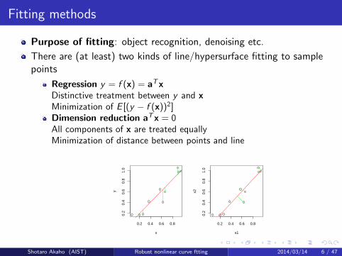
Purpose of fitting: object recognition, denoising etc.

There are (at least) two kinds of line/hypersurface fitting to samplepoints

Regression y = f (x) = aTxDistinctive treatment between y and xMinimization of E [(y − f (x))2]Dimension reduction aTx = 0All components of x are treated equallyMinimization of distance between points and line

0.2 0.4 0.6 0.8

0.2

0.4

0.6

0.8

1.0

x

y

0.2 0.4 0.6 0.8

0.2

0.4

0.6

0.8

1.0

x1

x2


. . . . . .

Fitting by dimension reduction

Minimization of distance between points and subspace (MCA)

Equivalently, find the subspace that preserves variance of data pointsas much as possible (PCA)

Equivalence of Principal Component Analysis (PCA) and MinorComponent Analysis (MCA)

Solution is obtained by solving eigenvalue problem

(XTX )a = λa


. . . . . .

Extension to Riemannian space

In many applications, we need to consider non-Euclidean space

Hypersphere (directional data, geology, economics; Fujiki+2007)

Grassmann-Stiefel manifold (subspace data, independent componentanalysis; Nishimori+2005)

Statistical manifold (statistics, optimization, control; Akaho2004)


. . . . . .

Extension to Riemannian space

Riemannian space with metric G (x)

Extension to distance to the length of geodesic (hard to evaluate)

Local approximation by the norm on the tangent space at xi∥x− xi∥2Gi

= (x− xi )TGi (x− xi ), Gi = G (xi )

In spite of this approximation, dimension reduction problem cannot besolved by a simple eigenvalue problem.


. . . . . .

Table of contents







. . . . . .

Quadratic curve fitting

Quadratic curve fitting

a0 + a1x1 + a2x2 + a3x21 + a4x1x2 + a5x

22 = 0

Feature map reduces the nonlinear problem to linear problemx 7→ ϕ(x) = (1, x1, x2, x1

2, x1x2, x22)

Linear fitting on 6 dimensional feature space


. . . . . .

Input space versus feature space

Linear method on feature space minimizes the distance in featurespace.

However, the distance is not equal to the distance between points andthe curve in the input space

There are not many researches focusing on input space (Scholkopf1999)


. . . . . .

Locally linear approximation of function

Projection from a point to a curve is difficult in general(local minimum/maximum, saddle)

Linear approximation of f (x∗i ) = 0 around xi(Akaho1993)

0 = f (x∗i ) ≃ f (xi ) +∇f (xi )T (x∗i − xi )

The closest point x∗i to xi w.r.t. metric Gi , satisfying the constraintabove is given by

∥x∗i − xi∥2Gi=

f (xi )2

∥∇f (xi )∥2G−1i


. . . . . .

Locally linear approximation of function

Applying to f (x) = aTϕ(x) leads to the sum of input space distance

∑i

∥x∗i − xi∥2Gi=

∑i

aTϕiϕTi a

aT∇ϕiG−1i ∇ϕT

i a, ϕi = ϕ(xi )

Sum of ratio of quadratic forms

Successive iteration method

at+1 = argmin∥a∥=1

aT

[∑i

1

wiϕiϕ

Ti

]a, wi = aTt ∇ϕiG

−1i ∇ϕT

i at ,


. . . . . .

Example

u ∼ u[−2, 2], x1 = u + ϵ1, x2 = u2 + ϵ2

-5 0 5

0

5

10

-5 0 5

0

5

10

Feature space Input space


. . . . . .

Table of contents







. . . . . .

Toward higher dimensions

Higher dimensional case (e.g. Reproducing Kernel Hilbert Space)

First, we consider support vector machine (not curve fitting, but findsoptimal separating hypersurface)

Fitting problem is discussed later


. . . . . .

Support vector machine

SVM finds an optimal hyperplane that maximizes margin in thefeature space

Maximize the margin in the input space by the approximation ofdistance in the input space

Approach: the same formulation as conventional SVM exceptintroducing a linear approximation of distance (+ additional linearexpansions; Akaho2004)

w Φ(x)=1

w Φ(x)=-1

w Φ(x)=0


. . . . . .

Approximation of distance

Approximate the distance not around xi but abetter estimate xi

∥di∥2Gi=

(aTϕ(xi )−∇ϕ(xi )di)2

∥aT∇ϕ(xi )∥2G−1i

di = x∗i − xi , di = xi − xi

xi is initialized by xi and it can be iterativelyimproved (discussed later)

xi

xi

xi

f(x)=0

^

*

di

di


. . . . . .

Margin constraint

Separating hyperplane is invariant under scalar transformation of a, sowe assume

mini

∥di∥2Gi=

1

∥a∥2

Then maximizing margin is equivalent to minimizing ∥a∥2 (quadraticregularization) under the above constraints with sign

yiaTϕ(xi )−∇ϕ(xi )di)

∥aT∇ϕ(xi )∥2G−1i

≥ 1

∥a∥


. . . . . .

Linearization of constraints

Suppose an approximate solution a is given, we approximate theconstraint by linear inequality of a

aT [yiϕ(xi )−∇ϕ(xi )di − ηi ] ≥ gi

where gi : scalar function, ηi : linear function of ∇ϕ(xi ) and a

Quadratic optimization with linear constraint leads to

L(a) = aTa−n∑

i=1

αi

(aT [yiϕ(xi )−∇ϕ(xi )di − ηi ]− gi

)where αi is a Lagrange multiplier


. . . . . .

Support Vectors

Differentiating L(a) by a, we have

a =n∑

i=1

αi [yiϕ(xi )−∇ϕ(xi )di − ηi ]

Sparsity (some αi are exactly 0 as in SVM)

Classification function f (x) = aTϕ(x):if we assume a is a linear function of ϕ(xi ) and ∇ϕ(xi ),

f (x) =∑i

aiϕ(xi )Tϕ(x) + bi∇ϕ(xi )Tϕ(x)

(Since ηi is a linear function of a and ϕ(xi ))


. . . . . .

Kernelization

Reproducing kernel Hilbert space

Kernel function (strictly it should be written as an inner product)

k(x, x′) = ϕ(x)Tϕ(x′)

Derivative of kernel function

∇xk(x, x′) = ∇ϕ(x)Tϕ(x′),

∇x∇x′k(x, x′) = ∇ϕ(x)T∇ϕ(x′)


. . . . . .

Kernel trick

Kernel trick enables us to choose positive semidefinite function as akernel function instead of taking inner product in the feature space

Example (Gaussian kernel)

k(x, x′) = exp(−β∥x− x′∥2)∇xk(x, x′) = −2βk(x, x′)(x− x′),∇x∇x′k(x, x′) = 2βk(x, x′)(I − 2β(x− x′)(x− x′)T ),

Kernel version of classification function

f (x) =∑i

aik(xi , x) + bi∇k(xi , x)


. . . . . .

Estimation of xi

xi can be improved for a fixed parameter of curve a

x[l+1]i = h(x

[l ]i , a, xi ,Gi )

It may converge to a local minimum, a local maximum, or a saddlepoint. How about the convergence property?

Property of the iterative solution: Let x∗i be an equilibrium stateof the iteration step, it is a critical point of the projection point (alocal minimum/maximum, or saddle point). If it is a local maximumor saddle, the algorithm is always unstable


. . . . . .

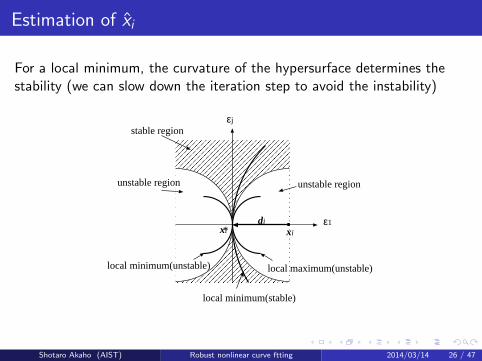
Estimation of xi

For a local minimum, the curvature of the hypersurface determines thestability (we can slow down the iteration step to avoid the instability)

stable region

unstable region

local maximum(unstable)

local minimum(stable)

local minimum(unstable)

unstable region

ε1xixi*

εj

di


. . . . . .

Example

Through experiments for synthetic and some benchmark datasets, weshowed that the input space margin and generalization performanceincreased by a proposed method

0 0.2 0.4 0.6 0.8 1

0

0.1

0.2

0.3

0.4

0.5

0.6

0.7

0.8

0 0.2 0.4 0.6 0.8 1−0.1

0

0.1

0.2

0.3

0.4

0.5

0.6

0.7

0.8

0.9

0 2 4 6 8 10 12

0.045

0.05

0.055

0.06

0.065

0.07

0.075

0.08

0.085

0.09

steps

Margin (input space)

Original Input space Margin


. . . . . .

Table of contents







. . . . . .

Robustness and sparseness

Typical optimization formulation for fitting

E =∑i

Cost(xi , f ) + λReg(f )

Regularization: we don’t discuss in detail hereSVM: L2, Lasso: L1 (sparse prior)

Cost:-SVM: Hinge loss of [yf (x)− 1]+-Ordinary regression: Quadratic loss (y − f (x))2

-Fitting by dimension reduction: Quadratic (vertical) distance-Here: p-th power (vertical) distance (robust + sparseness)


. . . . . .

p-th power deviation

Euclidean distance from a d-dim point xi to a hyperplaneaTx+ a0 = 0, ∥a∥ = 1 is given by |aTxi + a0|Minimizing the mean p-th power of the Euclidean distance

Rp(a) =n∑

i=1

wi |aTxi + a0|p

R1 norm (Ding2006)

R0 is meaningless (the same cost values)

We can prove Lp 0 < p ≤ 1 case is completely sparse (the optimalhyperplane passes through d points)


. . . . . .

Proof sketch

The parameter (aT , a0) is on a cylinder Q = Sd × R: convex in Rd+1

against the originParameter space is devided by n hyperplanes aTxi + a0 = 0, each P isconvex in Rd+1. ⇒ P ∩ Q is convex against the originThe (weighted) p-th deviation takes concave contour against originThe minimum of the objective function is obtained in the boundary ofP ∩ QThe procedure is performed recursively, and the (local) minimum isobtained at one of the vertex of P


. . . . . .

Example

−2 −1 0 1 2 3

02

46

8

Feature space (p = 0.5)

−2 −1 0 1 2 3

02

46

8

Input space (p = 0.5)(Yellow (Feature space p = 2) and Blue (Input space p = 2))


. . . . . .

Example


. . . . . .

Table of contents







. . . . . .

Curve fitting in RKHS

We want to extend the curve fitting in high dimensional space

PCA vs MCA (in low dimensional case, it is almost equivalent)

In infinite dimensional case, the difference taking higher eigenvaluesand discarding lower eigenvalues is large

Note: finding a dimension reduction map u = f (x) and finding a lowdimensional structure x ′ = g(x) in the input space are slightlydifferent


. . . . . .

Minor component analysis

In the first part of my talk, we considered the hyperplane aTϕ(x) = 0which is obtained by MCA

MCA is attractive because to find the optimal hyperplane wassomewhat reasonable in SVM

But in MCA case, it is hard because of too much degree of freedom


. . . . . .

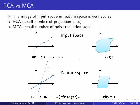
PCA vs MCA

The image of input space in feature space is very sparsePCA (small number of projection axes)MCA (small number of noise reduction axes)


. . . . . .

Two kinds of regularization

Tikhonov (SVM)

minf

∑i

Cost(f (xi )) + λΩ(∥f ∥)

f ∈ RKHS, Ω is a nondecreasing function

Ivanov-like (PCA, MCA) not precisely Ivanov

minf

∑i

Cost(f (xi )) s.t. ∥f ∥ = const


. . . . . .

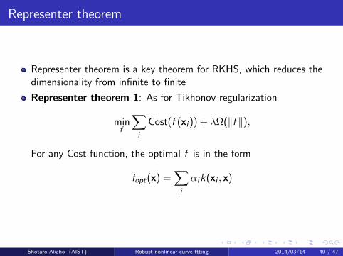
Representer theorem

Representer theorem is a key theorem for RKHS, which reduces thedimensionality from infinite to finite

Representer theorem 1: As for Tikhonov regularization

minf

∑i

Cost(f (xi )) + λΩ(∥f ∥),

For any Cost function, the optimal f is in the form

fopt(x) =∑i

αik(xi , x)


. . . . . .

Ivanov-like

Representer theorem 2: As for Ivanov-like regularization

minf

∑i

Cost(f (xi )) s.t. ∥f ∥ = const

If the Cost function satisfies decreasing property(Cost(c1f (x)) ≤ Cost(c2f (x)) when c1 ≥ c2 > 0), the optimal f is inthe form

fopt(x) =∑i

αik(xi , x)

PCA (minus of variance of f (xi )) satisfies, but MCA (variance off (xi )) does not! Even data out of samples can be good for MCA.


. . . . . .

Approach from PCA

Kernel PCA does not work as one would expect (cf. manifoldlearning)

For noise reduction, we need to solve “preimage problem” that isdifficult to solve

Even if preimage is found, it is not always what we want(non-smooth, more dimension is needed)

The structures of projection and preimage are different in nonlinearcase


. . . . . .

Preimage

Finding a dimension reduction map u = f (x) and finding a lowdimensional structure x ′ = g(x) in the input space are slightly different innonlinear case


. . . . . .

Example

Preimage is somewhat unstable and not smooth

−4 −2 0 2 4

−2

02

46

8

yt

xxxxxxxxxxxxxxxxxxxxxxxxxxxxxxxxxxxxxxxxxxxxxxxxxxxxxxxxxxxxxxxxxxxxxxxxxxxxxxxxxxxxxxxxxxxxxxxxxxxxxxxxxxxxxxxxxxxxxxxxxxxxxxxxxxxxxxxxxxxxxxxxxxxxxxxxxxxxxxxxxxxxxxxxxxxxxxxxxxxxxxxxx

xxxxxxxx xxxxxxx

xxxxxxxxxxxxxxxx

xxxx

xxxxxxxxxxxxxxxxxxxxxxxxxxxxxxxxxxxxxxxxxxxxxxxxxxxxxxxxxxxxxxxxxxxxxxxxxxxxxxxxxxxxxxxxxxxxxxxxxxxxxxxxxxxxxxxxxxxxxxxxxxxxxxxxxxxxxxxxxxxx

xxxxxxxxxxxxxxxxxxxx

−4 −2 0 2 4

−2

02

46

8

yt

xxxxxxxxxxxxx

xxxxxxx

xxxxxxxxxxxxx

xxxxxx

xxxxxxxxxxxxx

xxxxxx

xxxxxxxxxxxxx

xxxxxx

xxxxx xxxxxxx

xxxxxxxx

xxxx

x xx xx x xx

xxxxxxx

xxx

xxx x x x x

xxxxxxxxxx

xx

xxx x x x

xx

xxxxxxxxxx

xx

xx x x

xx

xxxxxxxxxxxx

xx

xx

xx

xxxxxxxxxxxxxxx

xx

x

x xxxxxxxxxxxxxxxx x

xx

xxxxxxxxxxxxxxxxx x xxxxxxxxxxxxxxxxxx x xxxxxxxxxxxxxxxxxxx xxxxxxxxxxxxxxxxxxx xxxxxxxxxxxxxxxxxx x xxxxxxxxxxxxxxxxxx x xxxxxxxxxxxxxxxxxx x xxxxxxxxxxxxxxxxxx x xxxxxxxxx

−4 −2 0 2 4

−2

02

46

8

yt

xxxxxxxxx xx xxxxxxxxx

xxxxxxx x x xx xxxxxxxx

xxxxxxx x x x x xxxxxxxx

xxxxxx x x x x x xxxxxxxxx

xxxx x x x x x x xxxxxxxxx

xxxxx x x x x x xxxxxxxxx

xxxxx x x x x xxxx

xxxxxx

xxxxxx x x x x

xxxxxxxxxx

xxx

x x x xx

xxxxxxxxxxxx

xxx

xx

xx

xxxxxxxxxxxxxxx

xx

x

x xxxxxxxxxxxxxxxx x

xx

xxxxxxxxxxxxxxxxx x xxxxxxxxxxxxxxxxxx x xxxxxxxxxxxxxxxxxx x xxxxxxxxxxxxxxxxxx x xxxxxxxxxxxxxxxxxx x

xxxxxxxxxxxxxxxxx x x xxxxxxxxxxxxxxxxxx xxxxxxxxxxxxxxxxxxx

xx xxxxxxxx

−4 −2 0 2 4

−2

02

46

8

yt

xxxxxxxxxxxxxxxxxxxxxx

xxxxxxxxxxxxxxxxxxxx

xxx xx xx xxxxxxxxxxxxxx

xx x x x x xxxxxxxxxxxxx

x x x x x x xxxxxxxxxxxxxx x x x x x xxxxxxxxxxxxxx x x x x xxxxxxxxxxxxxxxx x x x xxxxxxxxxxxxxxx x

x x x xxxxxxxxxxxxxxx x x

x x xxxxxxxxxxxxxxxx x x

x xxxxxxxxxxxxxxxx x x x

xxxxxxxxxxxxxxxx x x x x

xxxxxxxxxxxxxxx x x x xxxxxxxxxxxxxxxxx x xxxxxxxxxxxxxxxxxx x xxxxxxxxxxxxxxxxxx xxxxxxxxxxxxxxxxxxx xxxxxxxxxxxxxxxxxxx xxxxxxxxxxxxxxxxxxx xxxxxxxxxx


. . . . . .

Approach from MCA

Kernel MCA achieves smoother curve/surface

Too many freedom (even in the sample space)


. . . . . .

Example

MCA gives too many good curves! (their linear combination as well;Fujiki+2013)Further out of sample points will increase the freedomDoes sparsity help to choose a good curve? → open

−0.00032

−0.00032

−0.00071

−0.00071

−0.00071

−0.0013

−0.0013

0

0.00032 0.00032

0.00071

0.00071

0.0013

−4 −2 0 2 4

−2

02

46

8

−8.3e−05

−8.3e−05

−0.00021

−0.00021

−0.00052

−0.00052

0

0

8.3e−05

8.3e−05

0.00021

0.00021

0.00021

0.00052

−4 −2 0 2 4

−2

02

46

8

−4.6e−05

−4.6e−05

−0.00011

−0.00011

−0.00011

−0.00011

−0.00017

−0.00017 −0.00017

−0.00017

0

0

4.6e−05

4.6e−05

0.00011

0.00011

0.00017

0.00017

−4 −2 0 2 4

−2

02

46

8

−2.5e−05

−2.5e−05

−7.2e−05

−0.00019

0

0

2.5e−05

2.5e−05

7.2e−05

7.2e−05

0.00019

0.00019

−4 −2 0 2 4

−2

02

46

8


. . . . . .

Concluding remarks

The method to incorporate input space metric is proposed

Finding the projection point to hypersurface is more stable thanfinding the preimage

Lp cost function is effective when many outliers exist

MCA has a potential to give a good curve fitting, but choosing a goodcurve obtaining good generalization performance is not established


on the robust nonlinear curve fitting - ism.ac.jpfukumizu/coopmathws2014/akaho_coopmathws... ·...

Documents