nonlinear curve fitting -...
TRANSCRIPT
1
Nonlinear Curve Fitting
Earl F. GlynnScientific Programmer
Bioinformatics
11 Oct 2006
2
Nonlinear Curve Fitting• Mathematical Models• Nonlinear Curve Fitting Problems
– Mixture of Distributions– Quantitative Analysis of Electrophoresis Gels– Fluorescence Correlation Spectroscopy (FCS)– Fluorescence Recovery After Photobleaching (FRAP)
• Linear Curve Fitting• Nonlinear Curve Fitting
– Gaussian Case Study– Math– Algorithms– Software
• Analysis of Results– Goodness of Fit: R2
– Residuals• Summary

3
Mathematical Models
• Want a mathematical model to describe observations based on the independent variable(s) under experimental control
• Need a good understanding of underlying biology, physics, chemistry of the problem to choose the right model
• Use Curve Fitting to “connect” observed data to a mathematical model
4
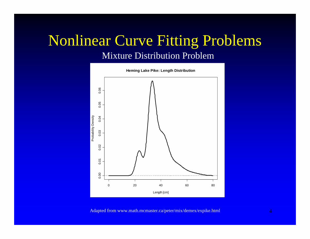
Nonlinear Curve Fitting ProblemsMixture Distribution Problem
Adapted from www.math.mcmaster.ca/peter/mix/demex/expike.html
0 20 40 60 80
0.00
0.01
0.02
0.03
0.04
0.05
0.06
Heming Lake Pike: Length Distribution
Length [cm]
Pro
babi
lity
Den
sity
5
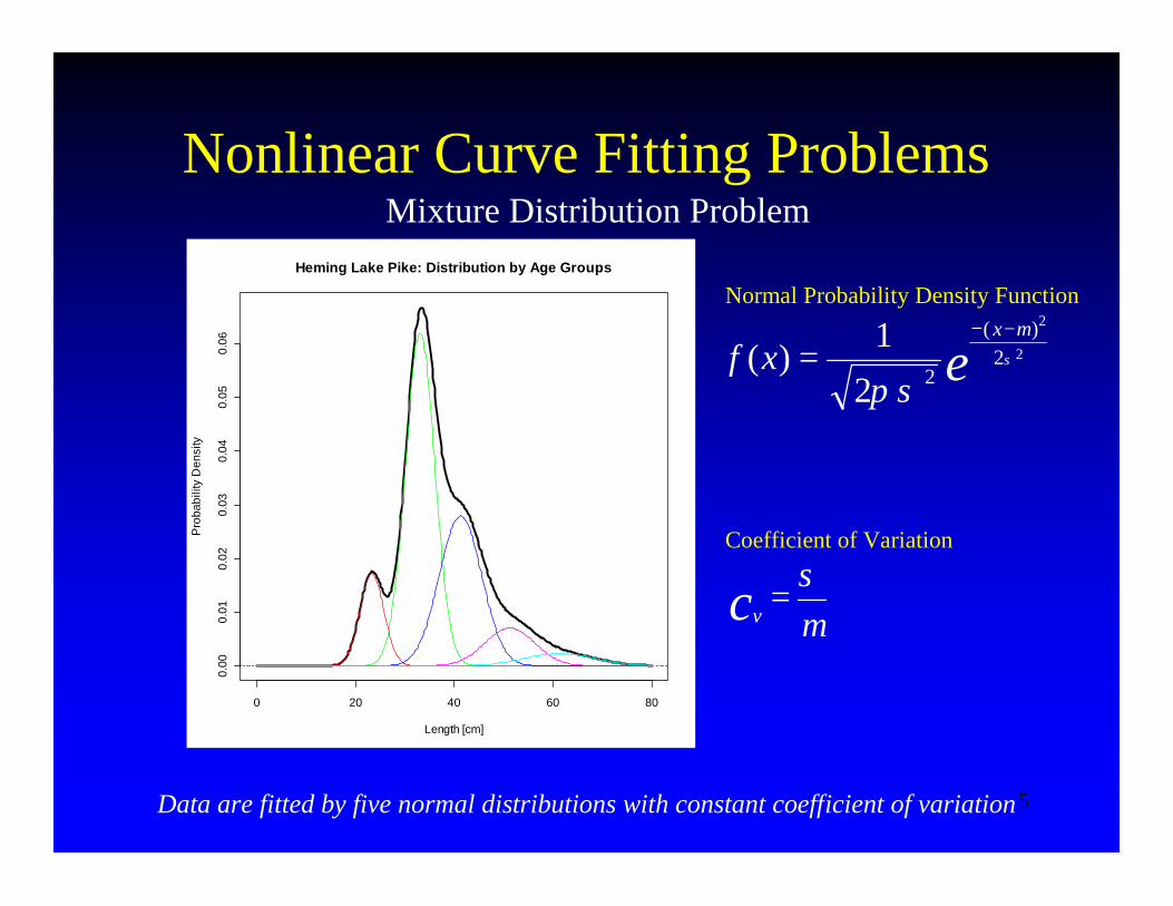
Nonlinear Curve Fitting ProblemsMixture Distribution Problem
Data are fitted by five normal distributions with constant coefficient of variation
0 20 40 60 80
0.00
0.01
0.02
0.03
0.04
0.05
0.06
Heming Lake Pike: Distribution by Age Groups
Length [cm]
Pro
babi
lity
Den
sity
ex
xf σ
µ
σπ2
2
2)(
221)(
−−
=
Normal Probability Density Function
Coefficient of Variation
µσ
=cv
6
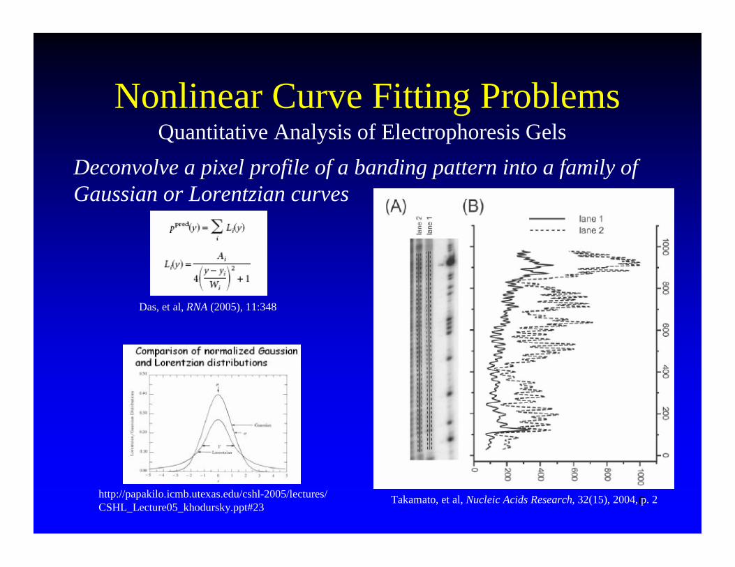
Deconvolve a pixel profile of a banding pattern into a family of Gaussian or Lorentzian curves
Quantitative Analysis of Electrophoresis Gels
Takamato, et al, Nucleic Acids Research, 32(15), 2004, p. 2
Nonlinear Curve Fitting Problems
http://papakilo.icmb.utexas.edu/cshl-2005/lectures/CSHL_Lecture05_khodursky.ppt#23
Das, et al, RNA (2005), 11:348
7
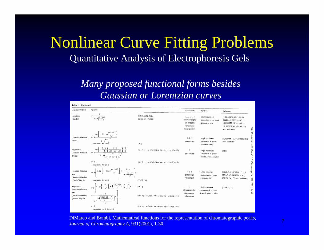
Nonlinear Curve Fitting ProblemsQuantitative Analysis of Electrophoresis Gels
Many proposed functional forms besides Gaussian or Lorentzian curves
DiMarco and Bombi, Mathematical functions for the representation of chromatographic peaks,Journal of Chromatography A, 931(2001), 1-30.
8
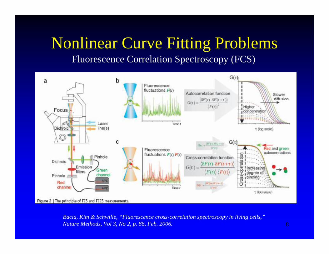
Nonlinear Curve Fitting ProblemsFluorescence Correlation Spectroscopy (FCS)
Bacia, Kim & Schwille, “Fluorescence cross-correlation spectroscopy in living cells,”Nature Methods, Vol 3, No 2, p. 86, Feb. 2006.
9
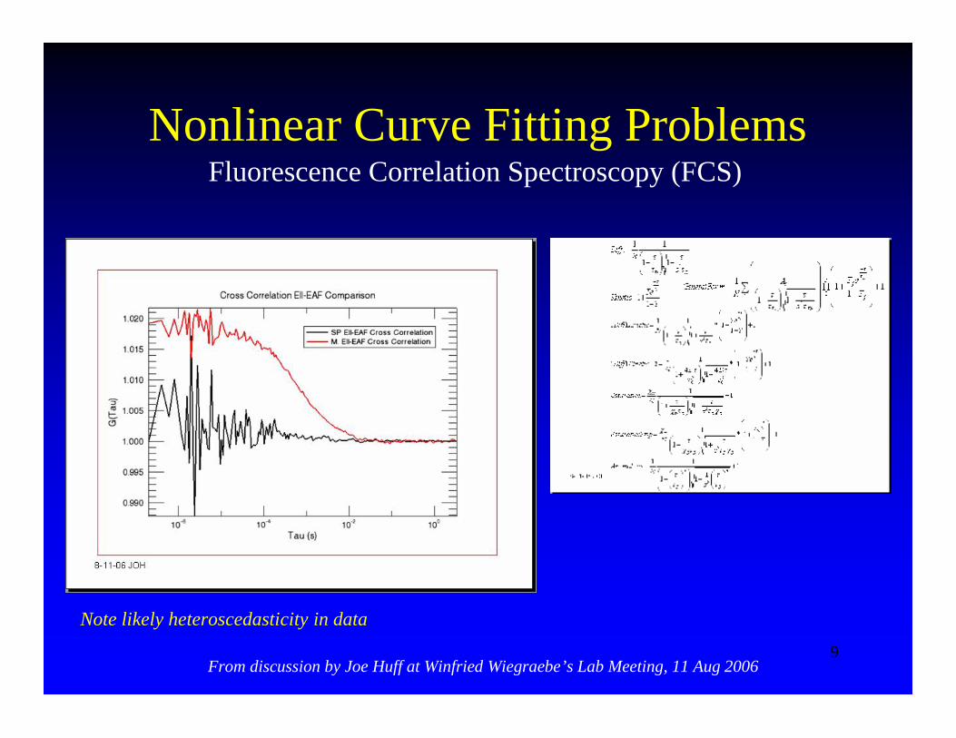
Nonlinear Curve Fitting ProblemsFluorescence Correlation Spectroscopy (FCS)
From discussion by Joe Huff at Winfried Wiegraebe’s Lab Meeting, 11 Aug 2006
Note likely heteroscedasticity in data

10
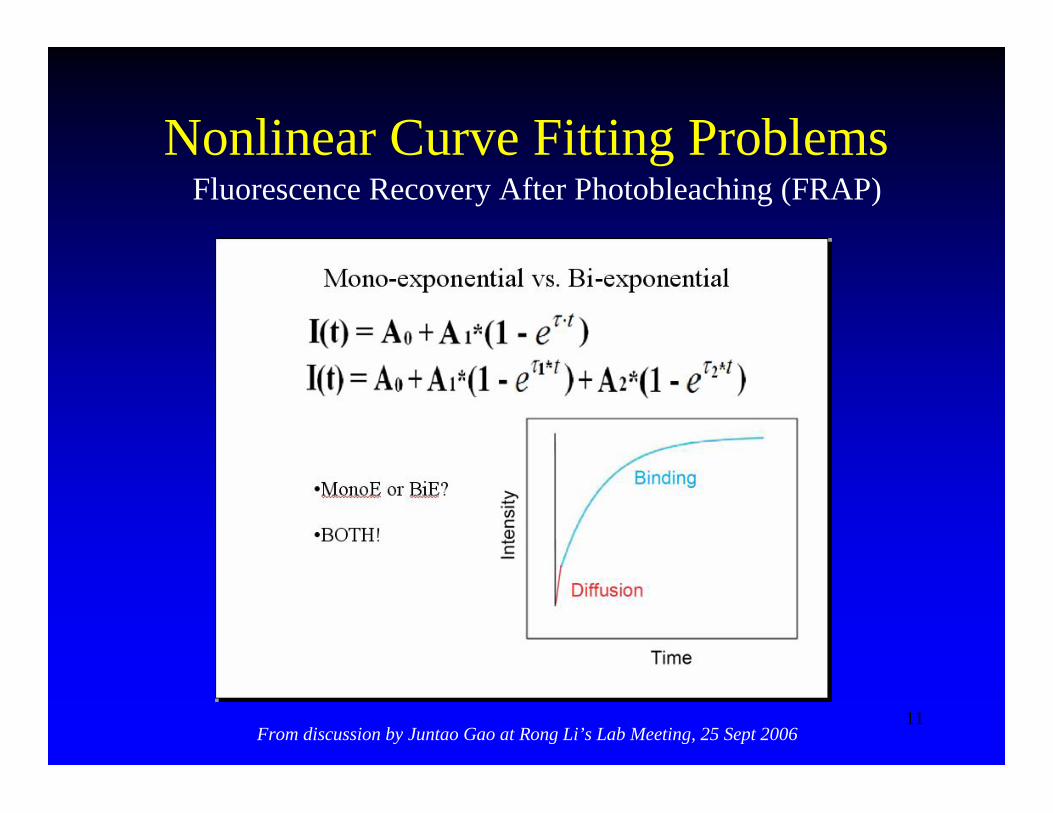
Nonlinear Curve Fitting ProblemsFluorescence Recovery After Photobleaching (FRAP)
From discussion by Juntao Gao at Rong Li’s Lab Meeting, 25 Sept 2006
11
Nonlinear Curve Fitting ProblemsFluorescence Recovery After Photobleaching (FRAP)
From discussion by Juntao Gao at Rong Li’s Lab Meeting, 25 Sept 2006
12
Linear Curve Fitting
• Linear regression• Polynomial regression• Multiple regression• Stepwise regression• Logarithm transformation
13
Given data points ( , ).
We want the “best” straight line, ( , ),through these points, where is the“fitted”value at point :
xixi
yi
Linear Regression: Least Squares
yiˆ
xy ii ba +=ˆ
yiˆ
Linear Curve Fitting
14
xixi
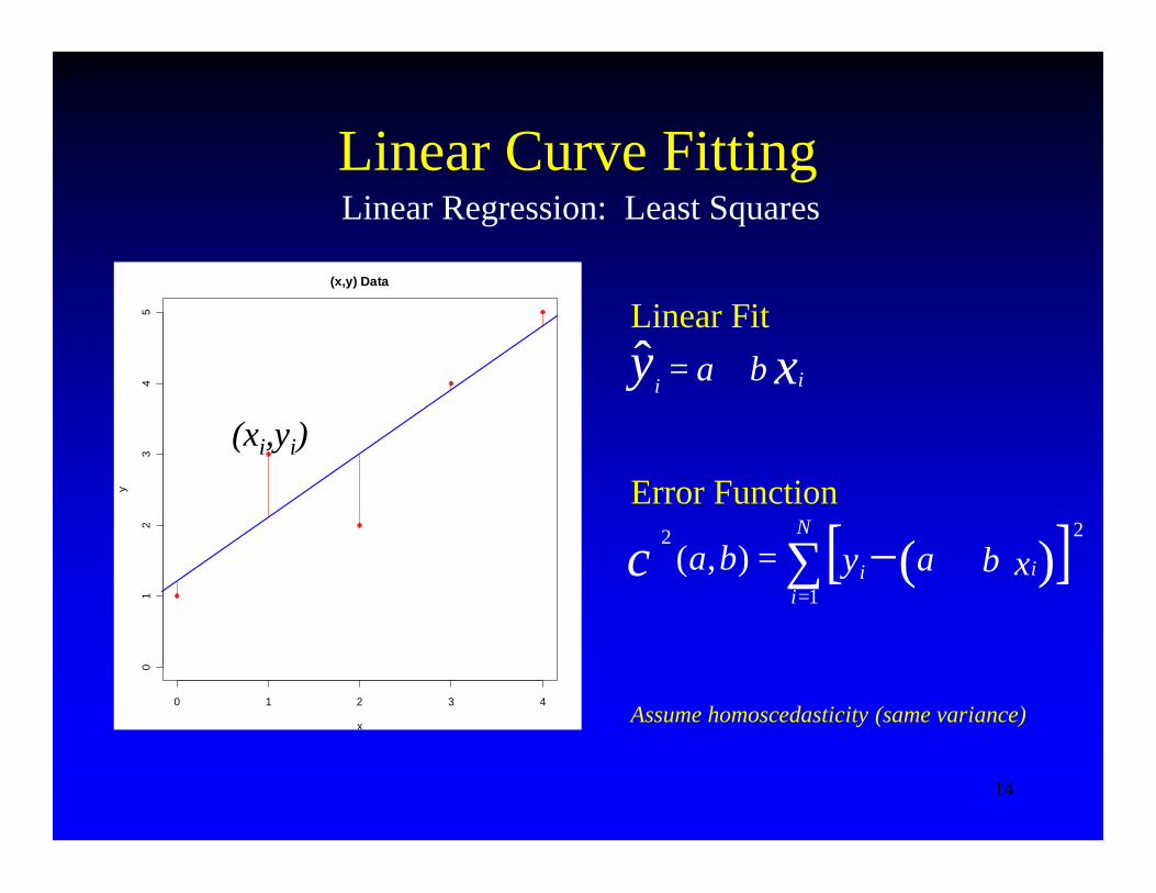
Linear Regression: Least Squares
xy ii ba +=ˆ
0 1 2 3 4
01
23
45
(x,y) Data
x
y
Linear Curve Fitting
Linear Fit
Error Function
[ ]∑ ⋅+−=
=N
iii xbayba
1
22 )(),(χ
(xi,yi)
Assume homoscedasticity (same variance)
15
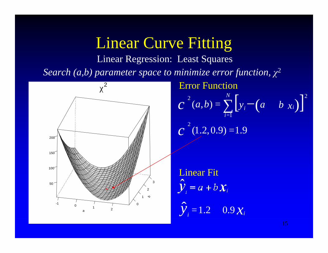
Search (a,b) parameter space to minimize error function, χ2
Linear Curve Fitting
b
0
1
2
3
a
-1 0 1 2
50
100
150
200
χ2 Error Function
[ ]∑ ⋅+−=
=N
iii xbayba
1
22 )(),(χ
Linear Fit
9.1)9.0,2.1(2
=χ
xy ii 9.02.1ˆ +=
Linear Regression: Least Squares
16
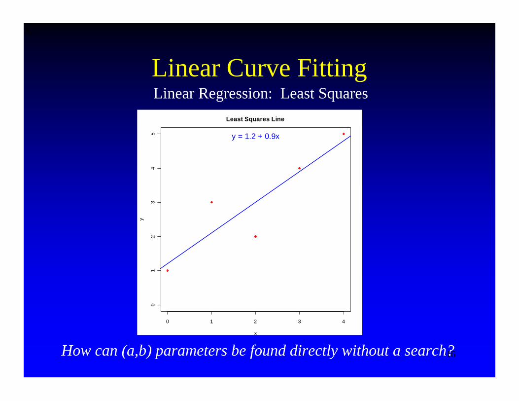
xixi
Linear Regression: Least SquaresLinear Curve Fitting
0 1 2 3 4
01
23
45
Least Squares Line
x
yy = 1.2 + 0.9x
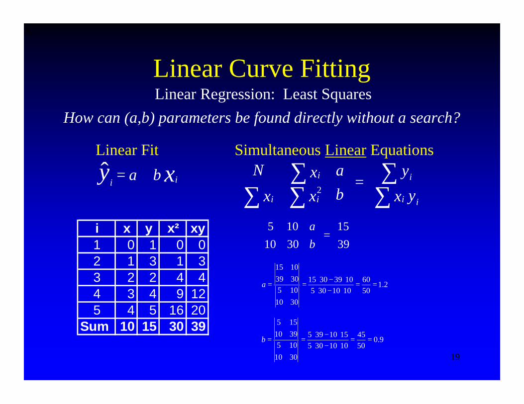
How can (a,b) parameters be found directly without a search?
17
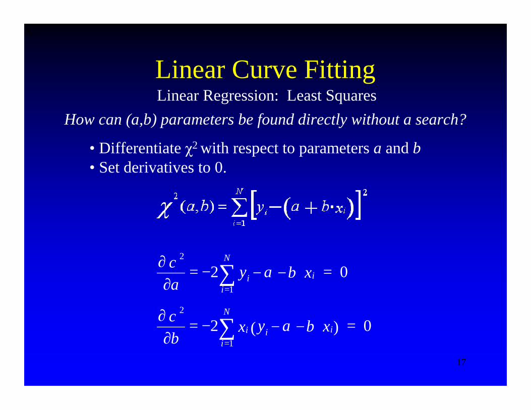
xixi
Linear Regression: Least Squares
• Differentiate χ2 with respect to parameters a and b• Set derivatives to 0.
Linear Curve Fitting
How can (a,b) parameters be found directly without a search?
021
2
=⋅−−−=∂
∂ ∑=
N
iii xbay
aχ
0)(21
2
=⋅−−−=∂
∂ ∑=
N
iii i xbayx
bχ
18
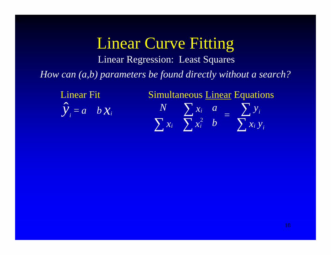
xixi
Linear Regression: Least SquaresHow can (a,b) parameters be found directly without a search?
xy ii ba +=ˆLinear Fit Simultaneous Linear Equations
Linear Curve Fitting
=
∑∑
∑∑∑
yxy
ba
xxxN
ii
i
ii
i2
19
xixi
Linear Regression: Least SquaresHow can (a,b) parameters be found directly without a search?
xy ii ba +=ˆLinear Fit
Linear Curve Fitting
=
∑∑
∑∑∑
yxy
ba
xxxN
ii
i
ii
i2
i x y x² xy1 0 1 0 02 1 3 1 33 2 2 4 44 3 4 9 125 4 5 16 20
Sum 10 15 30 39
=
3915
3010105
ba
2.15060
101030510393015
301010530391015
==⋅−⋅⋅−⋅
==a
9.05045
10103051510395
30101053910155
==⋅−⋅⋅−⋅
==b
Simultaneous Linear Equations
20
xixi
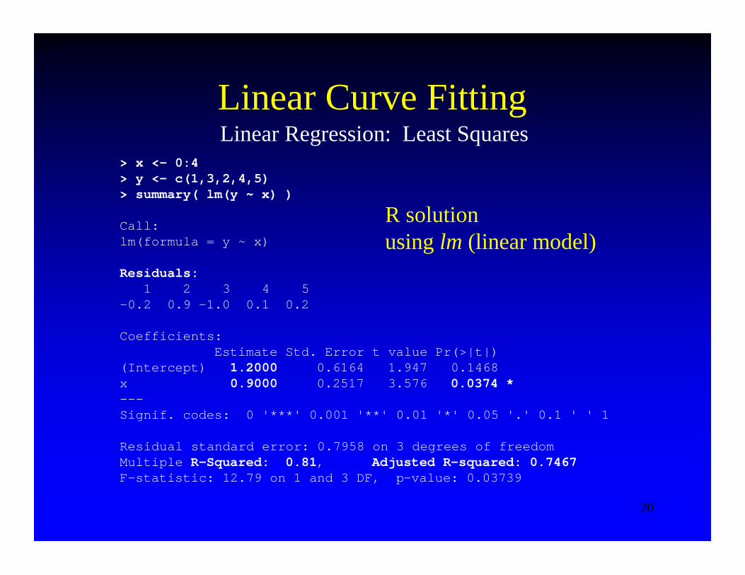
Linear Regression: Least SquaresLinear Curve Fitting
> x <- 0:4> y <- c(1,3,2,4,5) > summary( lm(y ~ x) )
Call:lm(formula = y ~ x)
Residuals:1 2 3 4 5
-0.2 0.9 -1.0 0.1 0.2
Coefficients:Estimate Std. Error t value Pr(>|t|)
(Intercept) 1.2000 0.6164 1.947 0.1468 x 0.9000 0.2517 3.576 0.0374 *---Signif. codes: 0 '***' 0.001 '**' 0.01 '*' 0.05 '.' 0.1 ' ' 1
Residual standard error: 0.7958 on 3 degrees of freedomMultiple R-Squared: 0.81, Adjusted R-squared: 0.7467F-statistic: 12.79 on 1 and 3 DF, p-value: 0.03739
R solutionusing lm (linear model)
21
xixi
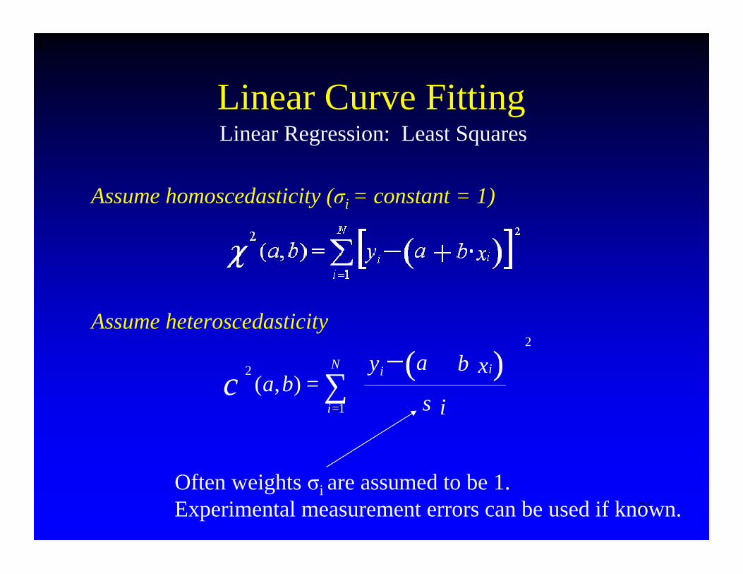
Linear Regression: Least SquaresLinear Curve Fitting
Assume homoscedasticity (σi = constant = 1)
Assume heteroscedasticity
∑
⋅+−
=
=N
i
ii
i
xbayba
1
2
2 )(),(
σχ
Often weights σi are assumed to be 1.Experimental measurement errors can be used if known.
22
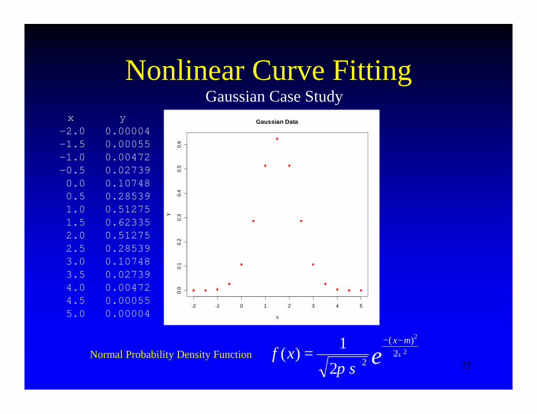
Nonlinear Curve Fitting
ex
xf σ
µ
σπ2
2
2)(
221)(
−−
=Normal Probability Density Function
Gaussian Case Study
-2 -1 0 1 2 3 4 5
0.0
0.1
0.2
0.3
0.4
0.5
0.6
Gaussian Data
x
y
x y-2.0 0.00004-1.5 0.00055-1.0 0.00472-0.5 0.027390.0 0.107480.5 0.285391.0 0.512751.5 0.623352.0 0.512752.5 0.285393.0 0.107483.5 0.027394.0 0.004724.5 0.000555.0 0.00004
23
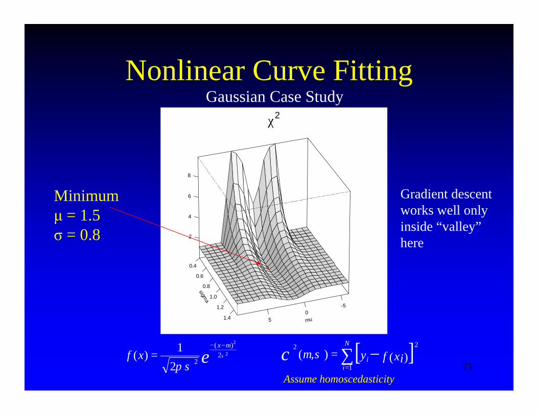
Nonlinear Curve Fitting
ex
xf σ
µ
σπ2
2
2)(
221)(
−−
= [ ]∑ −=
=N
ii xify
1
22
)(),( σµχ
mu
-50
5
sigma
0.4
0.6
0.8
1.0
1.2
1.4
2
4
6
8
χ2
Gaussian Case Study
Minimumμ = 1.5σ = 0.8
Gradient descentworks well onlyinside “valley”here
Assume homoscedasticity
24
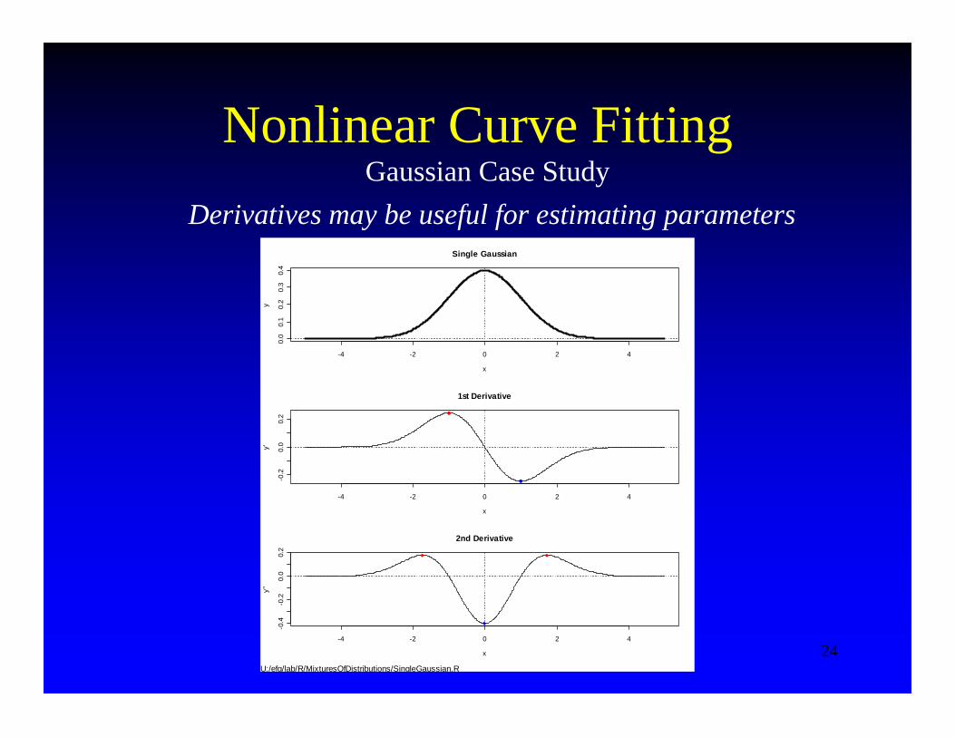
Nonlinear Curve FittingGaussian Case Study
Derivatives may be useful for estimating parameters
-4 -2 0 2 4
0.0
0.1
0.2
0.3
0.4
Single Gaussian
x
y
-4 -2 0 2 4
-0.2
0.0
0.2
1st Derivative
x
y'
-4 -2 0 2 4
-0.4
-0.2
0.0
0.2
2nd Derivative
x
y''
U:/efg/lab/R/MixturesOfDistributions/SingleGaussian.R
25
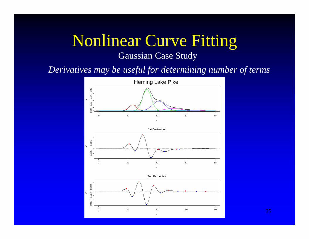
Nonlinear Curve FittingGaussian Case Study
Derivatives may be useful for determining number of terms
0 20 40 60 80
0.00
0.02
0.04
0.06
x
y
0 20 40 60 80
-0.0
050.
005
1st Derivative
x
y'
0 20 40 60 80
-0.0
06-0
.002
0.00
2
2nd Derivative
x
y''
Heming Lake Pike
26
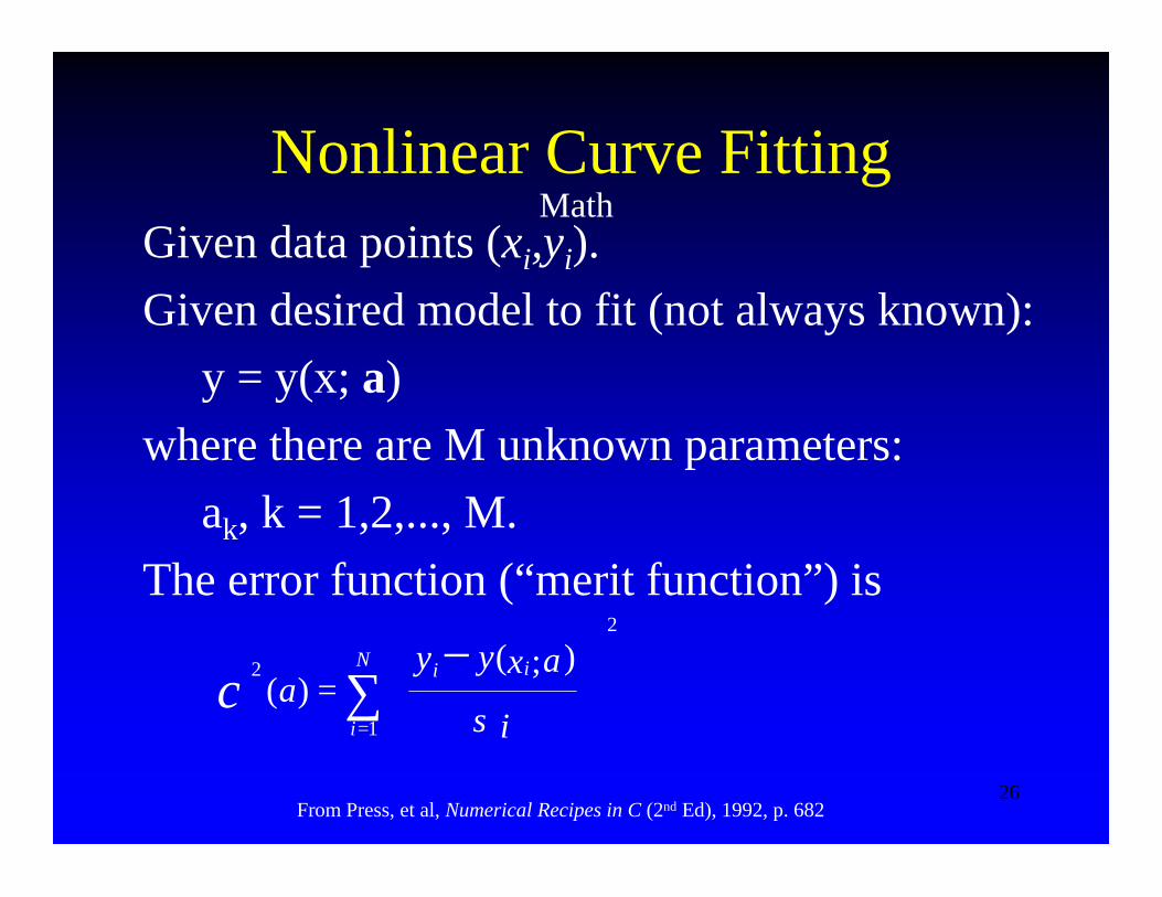
Nonlinear Curve FittingGiven data points (xi,yi).Given desired model to fit (not always known):
y = y(x; a)where there are M unknown parameters:
ak, k = 1,2,..., M.The error function (“merit function”) is
∑
−
=
=N
i
ii
i
axyya
1
2
2 );()(
σχ
From Press, et al, Numerical Recipes in C (2nd Ed), 1992, p. 682
Math
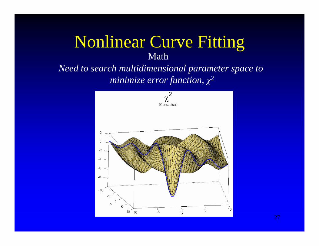
27
Need to search multidimensional parameter space to minimize error function, χ2
Nonlinear Curve FittingMath
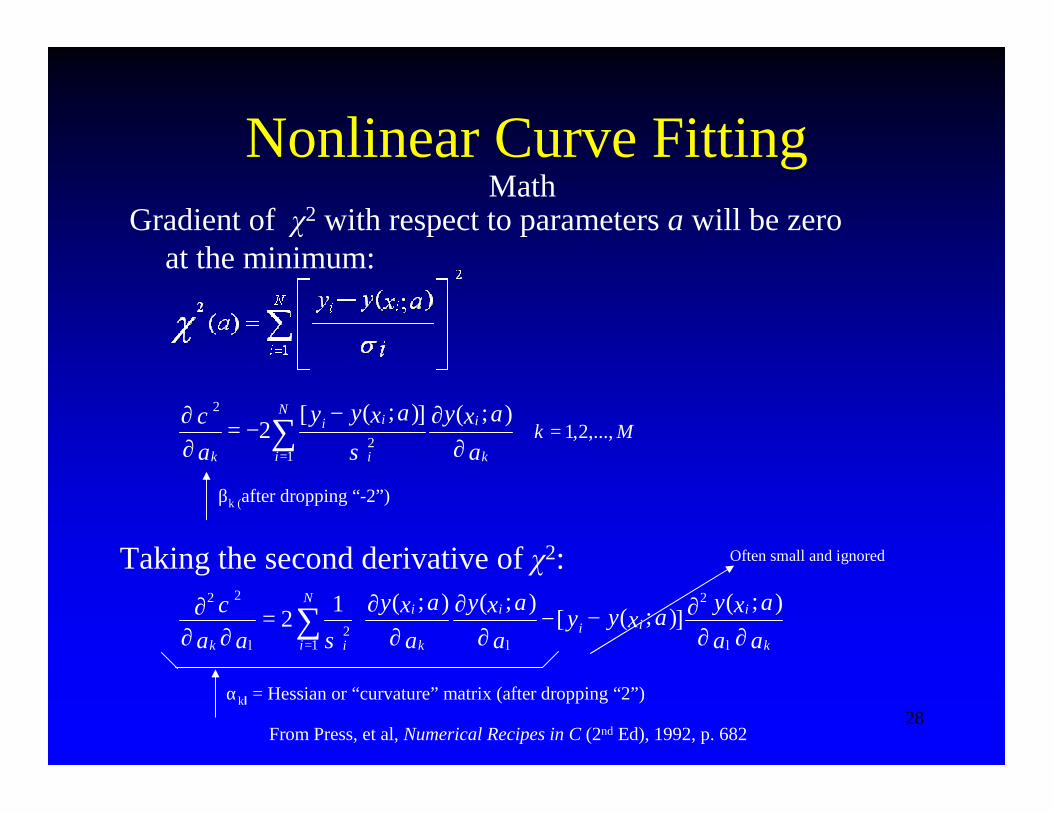
28
Gradient of χ2 with respect to parameters a will be zero at the minimum:
MkN
i k
i
i
ii
k aaxyaxyy
a,...,2,1
12
2 );(]);([2 =∑
= ∂∂−
−=∂∂
σχ
Nonlinear Curve Fitting
Taking the second derivative of χ2:
From Press, et al, Numerical Recipes in C (2nd Ed), 1992, p. 682
∑=
∂∂
∂−−∂
∂∂
∂=
∂∂∂ N
i k
iii
i
k
i
ik aaaxyaxyy
aaxy
aaxy
aa 1
2
2
22 );(]);([
);();(12lll σ
χ
αkl = Hessian or “curvature” matrix (after dropping “2”)
Often small and ignored
βk (after dropping “-2”)
Math
29
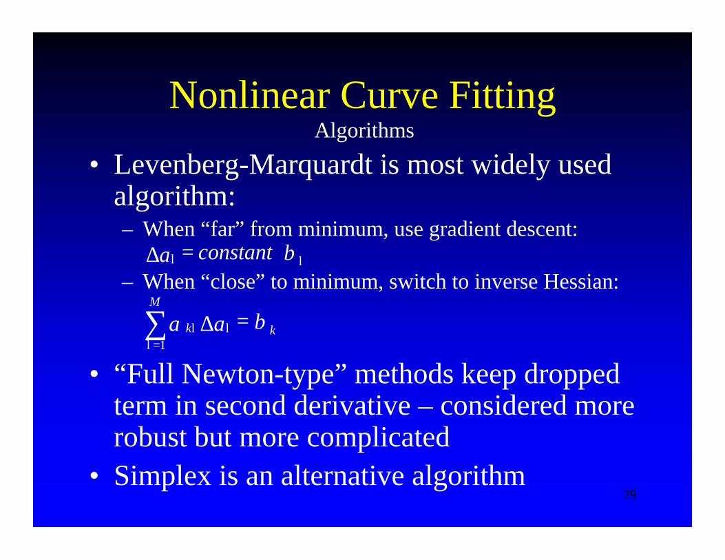
• Levenberg-Marquardt is most widely used algorithm:– When “far” from minimum, use gradient descent:
– When “close” to minimum, switch to inverse Hessian:
• “Full Newton-type” methods keep dropped term in second derivative – considered more robust but more complicated
• Simplex is an alternative algorithm
βα k
M
k a =∆∑=
l
l
l
1
β ll ⋅=∆ constanta
Nonlinear Curve FittingAlgorithms
30
Nonlinear Curve Fitting• Fitting procedure is iterative• Usually need “good” initial guess, based on
understanding of selected model• No guarantee of convergence• No guarantee of optimal answer• Solution requires derivatives: numeric or
analytic can be used by some packages
Algorithms
31
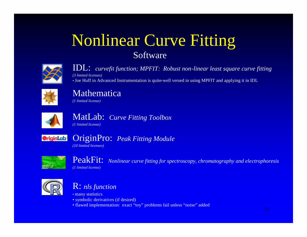
Nonlinear Curve FittingSoftware
IDL: curvefit function; MPFIT: Robust non-linear least square curve fitting(3 limited licenses)• Joe Huff in Advanced Instrumentation is quite-well versed in using MPFIT and applying it in IDL
R: nls function• many statistics• symbolic derivatives (if desired)• flawed implementation: exact “toy” problems fail unless “noise” added
MatLab: Curve Fitting Toolbox(1 limited license)
Mathematica(1 limited license)
PeakFit: Nonlinear curve fitting for spectroscopy, chromatography and electrophoresis(1 limited license)
OriginPro: Peak Fitting Module(10 limited licenses)
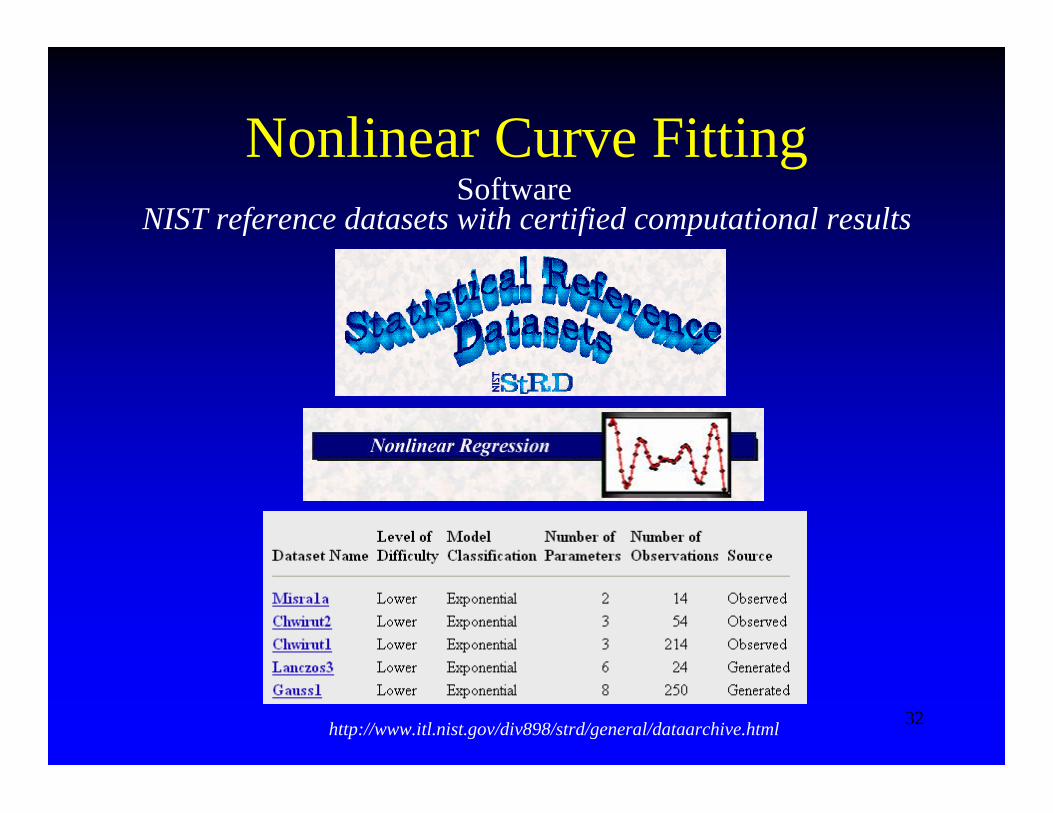
32http://www.itl.nist.gov/div898/strd/general/dataarchive.html
NIST reference datasets with certified computational results
Nonlinear Curve FittingSoftware
33
Analysis of Results• Goodness of Fit: R2
• Residuals
34
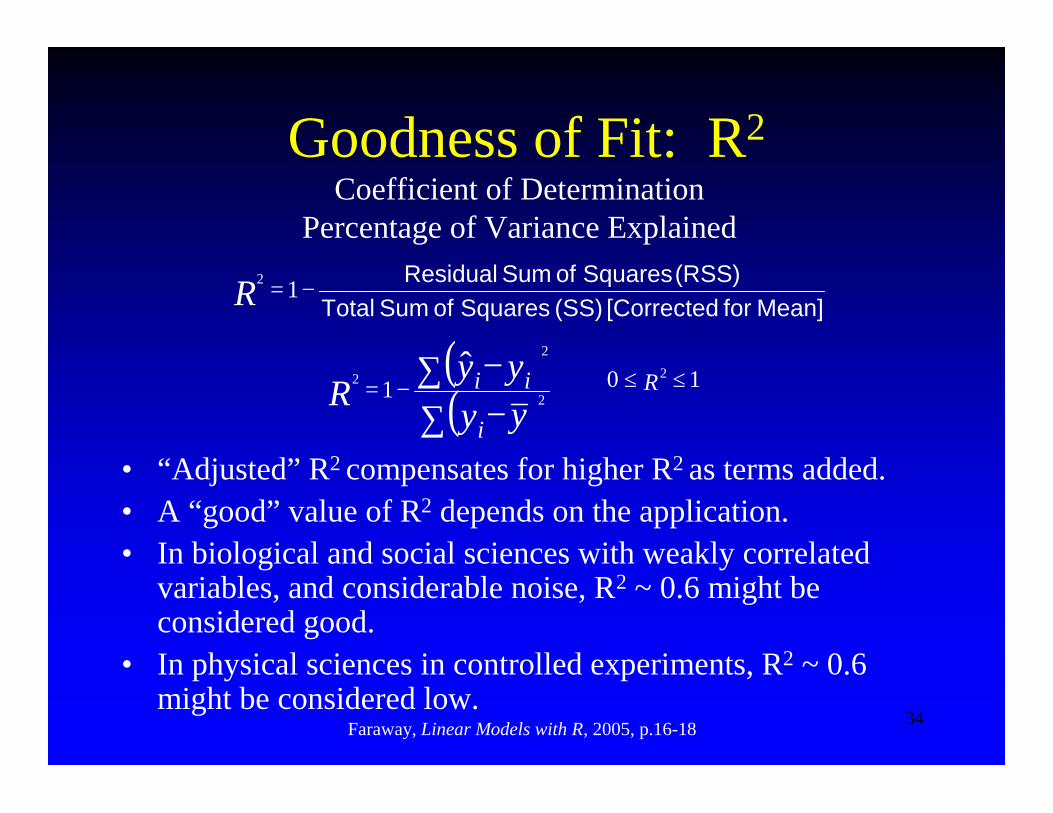
Goodness of Fit: R2Coefficient of Determination
Percentage of Variance Explained
Mean] for [Corrected (SS) Squares of Sum Total(RSS)Squares of Sum Residual
−= 12R
( )( )∑ −
∑ −−=
yyyy
Ri
ii2
2
2 ˆ1 10 2 ≤≤ R
• “Adjusted” R2 compensates for higher R2 as terms added. • A “good” value of R2 depends on the application.• In biological and social sciences with weakly correlated
variables, and considerable noise, R2 ~ 0.6 might be considered good.
• In physical sciences in controlled experiments, R2 ~ 0.6 might be considered low.
Faraway, Linear Models with R, 2005, p.16-18
35
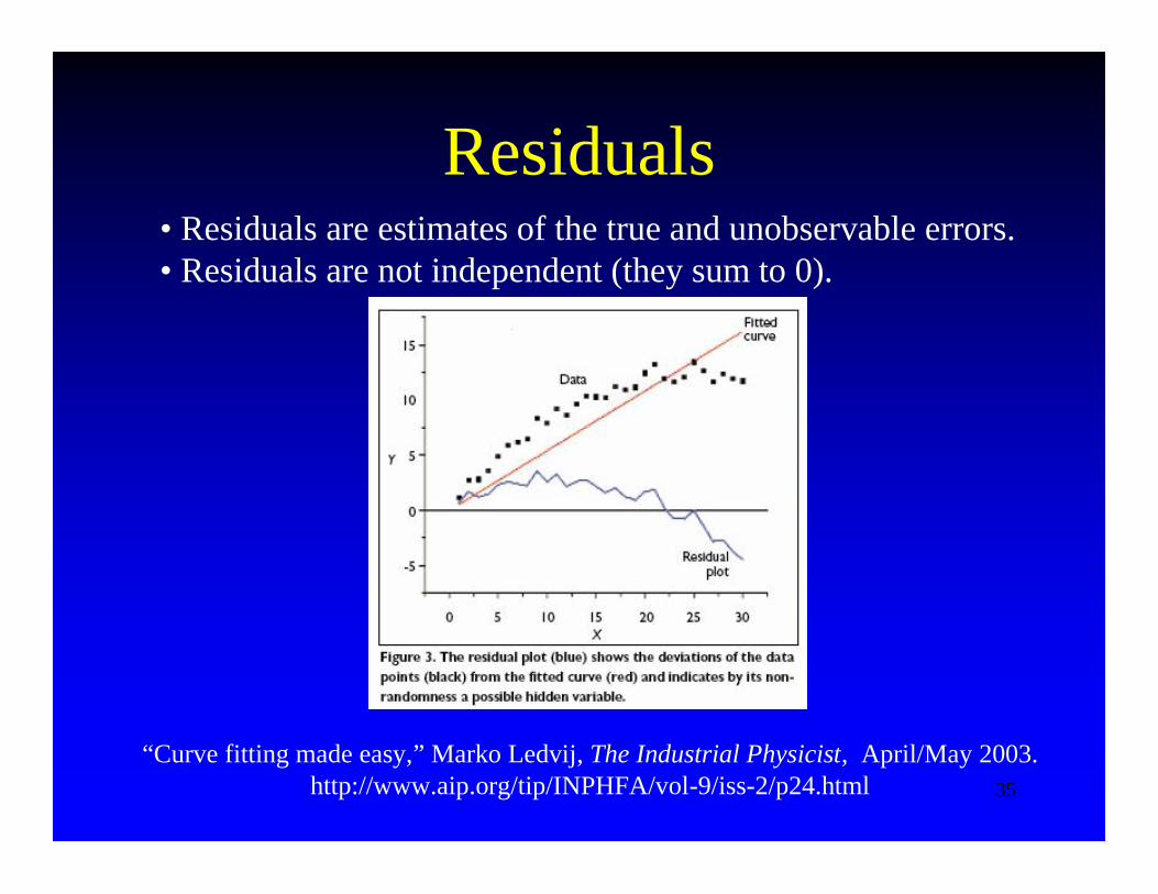
Residuals
“Curve fitting made easy,” Marko Ledvij, The Industrial Physicist, April/May 2003. http://www.aip.org/tip/INPHFA/vol-9/iss-2/p24.html
• Residuals are estimates of the true and unobservable errors.• Residuals are not independent (they sum to 0).
36
Analysis of Residuals
• Are residuals random?• Is mathematical model appropriate?• Is mathematical model sufficient to
characterize the experimental data?• Subtle behavior in residuals may suggest
significant overlooked propertyGood Reference: “Analysis of Residuals: Criteria for Determining Goodness-of-Fit,”Straume and Johnson, Methods in Enzymology, Vol. 210, 87-105, 1992.

37
Analysis of ResidualsSynthetic FRAP Data: Fit with 1 term when 2 terms are better
Near “perfect” fit, but why is there a pattern in the residuals?
38
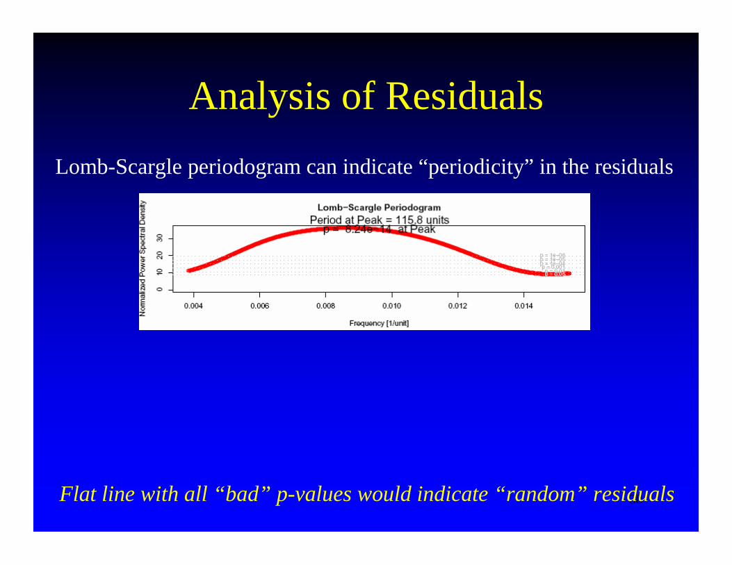
Analysis of ResidualsLomb-Scargle periodogram can indicate “periodicity” in the residuals
Flat line with all “bad” p-values would indicate “random” residuals
39
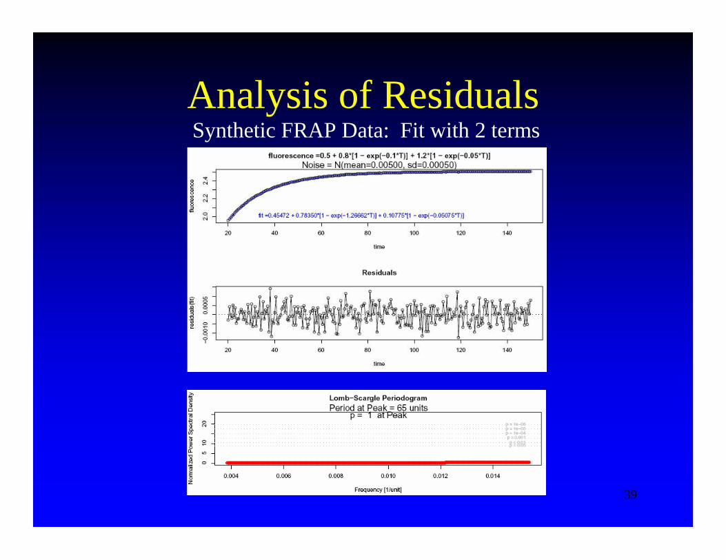
Analysis of ResidualsSynthetic FRAP Data: Fit with 2 terms
40
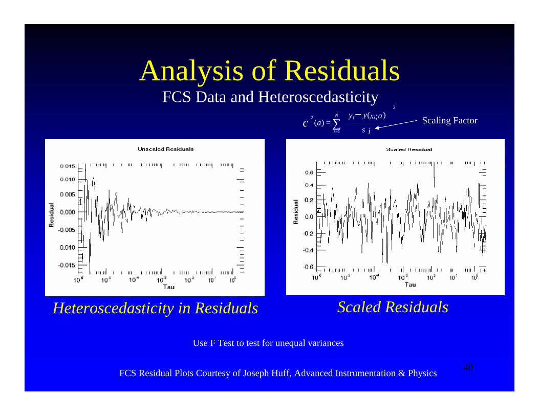
Analysis of ResidualsFCS Data and Heteroscedasticity
Heteroscedasticity in Residuals
∑
−
=
=N
i
ii
i
axyya
1
2
2 );()(
σχ
Scaled Residuals
Scaling Factor
FCS Residual Plots Courtesy of Joseph Huff, Advanced Instrumentation & Physics
Use F Test to test for unequal variances
41
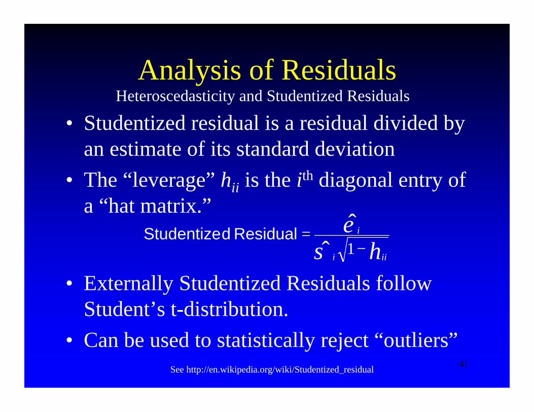
Analysis of ResidualsHeteroscedasticity and Studentized Residuals
See http://en.wikipedia.org/wiki/Studentized_residual
• Studentized residual is a residual divided by an estimate of its standard deviation
• The “leverage” hii is the ith diagonal entry of a “hat matrix.”
hiii
i
−=
1ˆˆ
σεResidualdStudentize
• Externally Studentized Residuals follow Student’s t-distribution.
• Can be used to statistically reject “outliers”
42
Summary• A mathematical model may or may not be appropriate for
any given dataset.• Linear curve fitting is deterministic.• Nonlinear curve fitting is non-deterministic, involves
searching a huge parameter space, and may not converge.• Nonlinear curve fitting is powerful
(when the technique works).• The R2 and adjusted R2 statistics provide easy to
understand dimensionless values to assess goodness of fit.• Always study residuals to see if there may be unexplained
patterns and missing terms in a model.• Beware of heteroscedasticity in your data. Make sure
analysis doesn’t assume homoscedasticity if your data are not.
• Use F Test to compare the fits of two equations.

43
AcknowledgementsAdvanced Instrumentation & Physics• Joseph Huff• Winfried Wiegraebe