parameter estimation for bayesian networkssrihari/cse674/chap17/17.1-bn...• parameter values with...

Machine Learning Srihari

1

Parameter Estimation for Bayesian Networks

Sargur Srihari [email protected]


Topics •  Problem Statement •  Maximum Likelihood Approach

– Thumb-tack (Bernoulli), Multinomial, Gaussian – Application to Bayesian Networks

•  Bayesian Approach – Thumbtack vs Coin Toss

•  Uniform Prior vs Beta Prior

– Multinomial •  Dirichlet Prior

2


Problem Statement •  BN structure is fixed •  Data set consists of M fully observed

instances of the network variables D ={ξ[1],…,ξ[M]}

•  Arises commonly in practice – Since hard to elicit from human experts

•  Forms building block for structure learning and learning from incomplete data

3


Two Main Approaches

1.  Maximum Likelihood Estimation 2.  Bayesian •  Discuss general principles of both •  Start with simplest learning problem

– BN with a single random variable – Generalize to arbitrary network structures

4


Thumbtack Example •  Simple Problem contains interesting issues

to be tackled: – Thumbtack is tossed to land head/tail

– Tossed several times obtaining heads or tails – Based on data set wish to estimate probability

that next flip will land heads/tails •  It is controlled by an unknown parameter: the

Probability of heads θ 5

heads tailsProbability of heads = θ


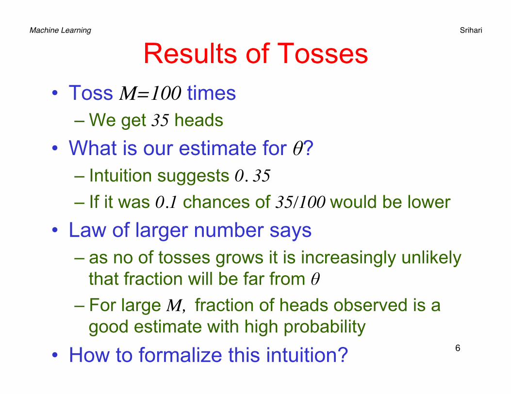
Results of Tosses •  Toss M=100 times

– We get 35 heads •  What is our estimate for θ?

–  Intuition suggests 0. 35–  If it was 0.1 chances of 35/100 would be lower

•  Law of larger number says – as no of tosses grows it is increasingly unlikely

that fraction will be far from θ – For large M, fraction of heads observed is a

good estimate with high probability •  How to formalize this intuition? 6


Maximum Likelihood Estimator •  Since tosses are independent, probability of

sequence is P(H,T,T,H,H:θ) =θ (1-θ)(1-θ) θθ =θ3(1-θ)2

•  Probability depends on value of θ •  Define the likelihood function to be

L(θ:<H,T,T,H,H>)=P(H,T,T,H,H:θ) =θ3(1-θ)2

•  Parameter values with higher likelihood are more likely to generate the observed sequences

•  Thus likelihood is measure of parameter quality

0 0.2 0.4 0.6 0.8 1

!!q"#""$

Llikelihood function for the sequence HTTHH

θ̂ = 0.6Since #H > #T it is >0.5


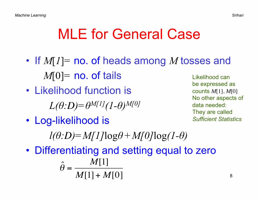
MLE for General Case

•  If M[1]= no. of heads among M tosses and M[0]= no. of tails •  Likelihood function is

L(θ:D)=θM[1](1-θ)M[0]

•  Log-likelihood is l(θ:D)=M[1]logθ +M[0]log(1-θ)

•  Differentiating and setting equal to zero

8 θ̂ =

M[1]M[1]+ M[0]

Likelihood can be expressed as counts M[1], M[0]No other aspects of data needed: They are called Sufficient Statistics


Limitations of Max Likelihood

•  If we get 3 heads out of 10 tosses, •  Same estimate if 300 heads out of 1,000 tosses

– Should be more confident with second estimate •  Statistical estimation theory deals with

Confidence Intervals – E.g., in election polls 61 + 2 percent plan to vote for

a certain candidate •  MLE estimate lies within 0. 2 of true parameter with high

probability 9

θ̂ = 0.3


Maximum Likelihood Principle •  Observe samples from unknown distribution

P*(χ) •  Training sample D consists of M instances of χ : {ξ[1],…,ξ[M]}

•  For a parametric model P(ξ;θ), we wish to estimate parameters θ

•  For each choice of parameter θ, P(ξ;θ) is a legal distribution

•  We need to define parameter space Θ which is the set of allowable parameters

P(ξ :θ) = 1ξ∑

Machine Learning Srihari Common Parameter Spaces

•  Thumb-tack •  X takes one of 2

values H, T •  Model •  P(x:θ )= θ if x =H

1-θ if x =T •  Parameter Space

Θthumbtack=[0,1] which is a probability

11

•  Multinomial •  X takes one of K

values x1..xK •  Model •  P(x:θ)=θk if x=xk

•  Parameter Space

•  Θmultinomial = {θ ∈[0,1]K :∑θi=1} a set of K probabilities

•  Gaussian •  X is continuous

on real line •  Model •  P(x:µ,σ)=

•  Parameter Space

•  ΘGaussian=R x R+

•  R: real value of µ •  R+: positive value σ

12πσ

e−(x−µ )2

2σ 2

Likelihood Function L(θ :D) = P(ξ[m] :θ)m∏


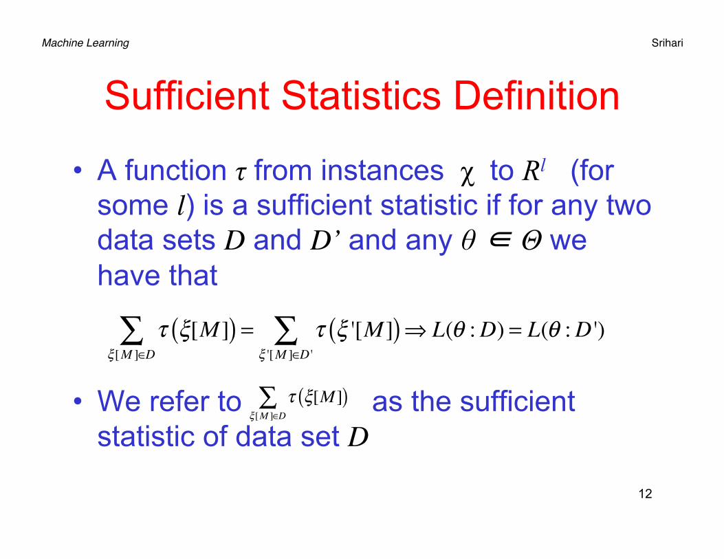
Sufficient Statistics Definition

•  A function τ from instances χ to Rl (for some l) is a sufficient statistic if for any two data sets D and D’ and any θ ∈ Θ we have that

•  We refer to as the sufficient statistic of data set D

12

τ ξ[M ]( )ξ[M ]∈D∑ = τ ξ '[M ]( )

ξ '[M ]∈D '∑ ⇒ L(θ :D) = L(θ :D ')

τ ξ[M ]( )ξ[M ]∈D∑

Machine Learning Srihari Sufficient Statistics Examples

•  In thumbtack – Likelihood is in terms of M[0] and M[1] which are

counts of 0s and 1s, L(θ:D)=θM[1](1-θ)M(0) •  No need for other aspects of training data e.g., toss order •  They are summaries of data for computing likelihood

•  For multinomial (with K values instead of 2) – Vector of counts M[1],..M[K] which are counts of xk

•  Number of times xk appears in training data

– Sum of instance level statistics •  obtained using τ(xk)=0,..0,1,0…0

– Likelihood function is 13 L(θ :D) = θk

M [k ]

k∏

1-of-K representation

Xii=1

N

∑ yields K-dim vector


Sufficient Statistics: Gaussian

14

PGaussian (x :µ,σ ) = e− x2

12σ 2

+ xµ

σ 2−µ2

2σ 2−12log(2π )− logσ

Likelihood function will involve ∑ xi2, ∑xi and ∑1

Sufficient statistic is the tuple sGaussian(x)= <1,x,x2> 1 does not depend on value of data item, but serves to count number of sample

From Gaussian model by expanding (x-μ)2 we can rewrite the model as

12πσ

e−(x−µ )2

2σ 2


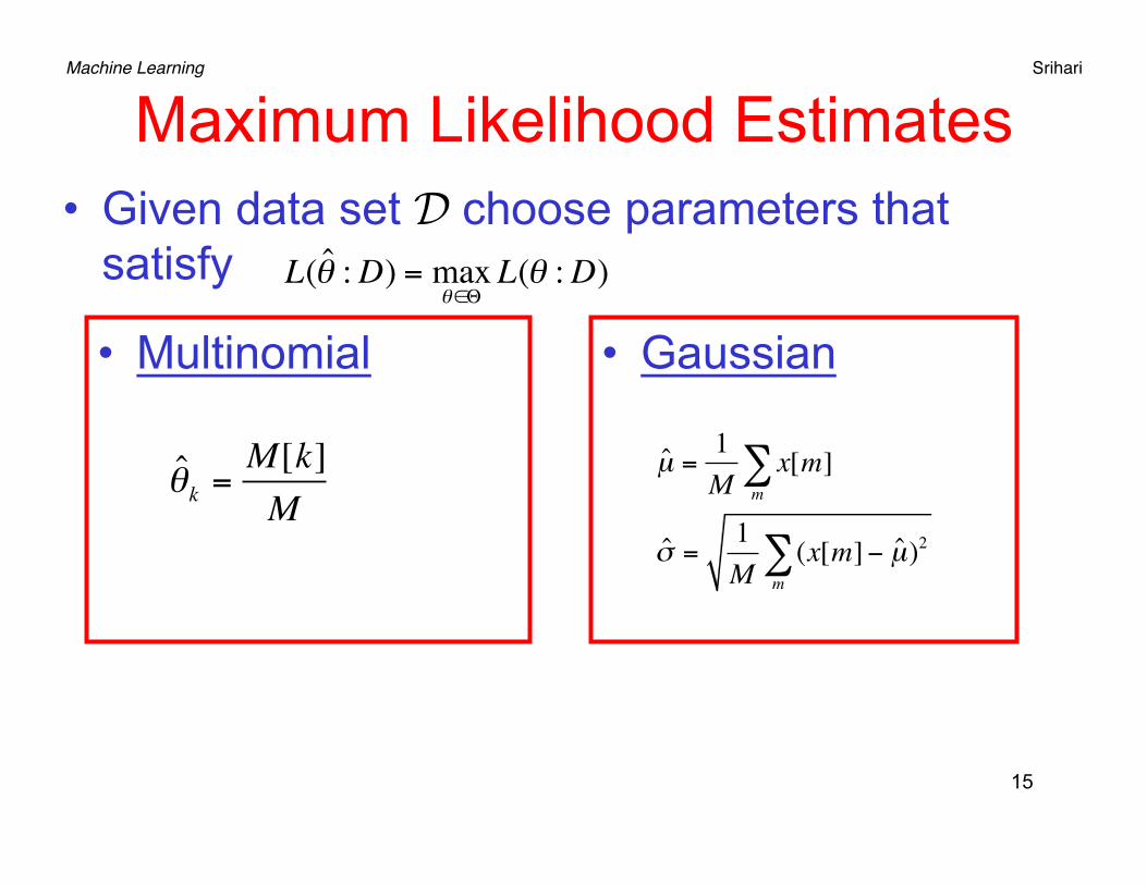
Maximum Likelihood Estimates •  Given data set D choose parameters that

satisfy

15

L(θ̂ :D) = maxθ∈Θ

L(θ :D)

•  Multinomial •  Gaussian

θ̂k =M[k]M

µ̂ =1M

x[m]m∑

σ̂ =1M

(x[m]− µ̂)2m∑


MLE for Bayesian Networks

•  Structure of Bayesian network allows us to reduce parameter estimation problem into a set of unrelated problems

•  Each can be addressed using methods described earlier

•  To clarify intuition consider a simple BN and then generalize to more complex networks

16


Simple Bayesian Network •  Network with two binary variables XàY •  Parameter vector θ defines CPD parameters •  Each training sample is a tuple <x[m],y[m]>

•  Network model specifies P(X,Y)=P(X)P(Y\X)

17

L(θ :D) = P(x[m], y[m] :θ)m=1

M

∏

L(θ :D) = P(x[m] :θ)m=1

M

∏ P(y | [m] | x[m] :θ)

changing order of multiplication

L(θ :D) = P(x[m] :θ)m=1

M

∏m=1

M

∏ P(y | [m] | x[m] :θ)

Likelihood decomposes into two separate terms, each a local likelihood function Measures how well variable is predicted given its parents


Global Likelihood Decomposition

•  A similar decomposition is obtained in general BNs

•  Leads to the conclusion: •  We can maximize each local likelihood

function independently of the rest of the network, and then combine the solutions to get an MLE solution

18


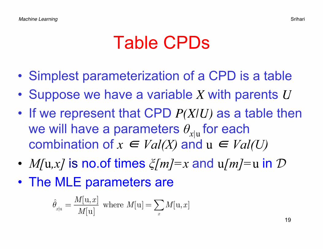
Table CPDs

•  Simplest parameterization of a CPD is a table •  Suppose we have a variable X with parents U•  If we represent that CPD P(X|U) as a table then

we will have a parameters θx|u for each combination of x ∈ Val(X) and u ∈ Val(U)

•  M[u,x] is no.of times ξ[m]=x and u[m]=u in D •  The MLE parameters are

19 θ̂

x|u=

M[u,x ]M[u]

where M[u] = M[u,x ]x∑


Challenge with BN parameter estimation

•  No. of data points used to estimate parameter is M[u]– estimated from samples with parent value u

•  Data points that do not agree with the parent assignment u play no role in this computation

•  As the no. of parents U grows, no of parent assignments grows exponentially – Therefore no. of data instances that we expect to

have for a single parent shrinks exponentially 20

θ̂x|u


Data Fragmentation problem

•  Data set is partitioned into a large number of small subsets

•  When we have a very small no. of data instances from which to estimate parameters – Yield noisy estimates leading to over-fitting – Likely to get a large no. of zeros leading to poor

performance •  Key limiting factor of learning BNs from data

21


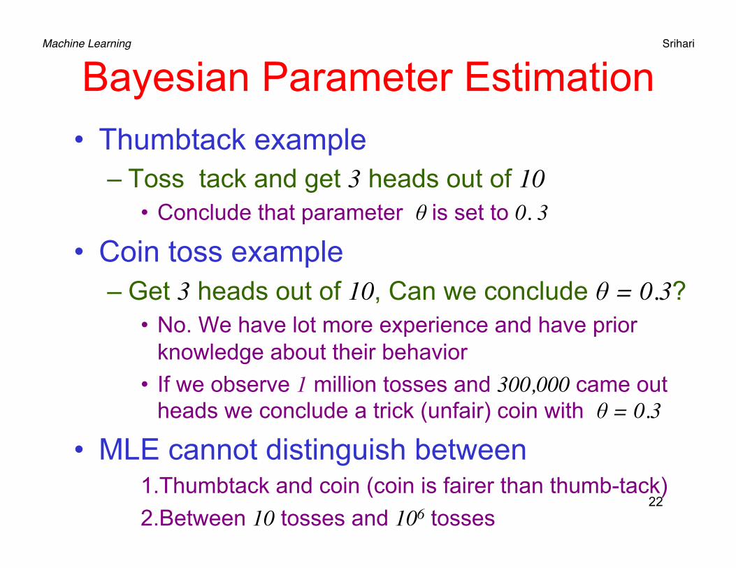
Bayesian Parameter Estimation •  Thumbtack example

– Toss tack and get 3 heads out of 10•  Conclude that parameter θ is set to 0. 3

•  Coin toss example – Get 3 heads out of 10, Can we conclude θ = 0.3?

•  No. We have lot more experience and have prior knowledge about their behavior

•  If we observe 1 million tosses and 300,000 came out heads we conclude a trick (unfair) coin with θ = 0.3

•  MLE cannot distinguish between 1. Thumbtack and coin (coin is fairer than thumb-tack) 2. Between 10 tosses and 106 tosses

22


Joint Probabilistic Model

•  Encode prior knowledge about θ with a probability distribution

•  Represents how likely we are about different choices of parameters

•  Create a joint distribution θ involving parameter and samples X [1] ,.. X [M]

•  Joint distribution captures our assumptions about experiment

23


Thumbtack Revisited

•  In MLE Tosses were assumed independent – Assumption made when θ was fixed

•  If we do not know θ then one toss tells us something about the parameter θ – Thus about next toss – Thus tosses are not marginally independent

•  Once we know θ we cannot learn probability of one toss from others – So tosses are conditionally independent given θ


Joint distribution of parameter and samples

qX

qX

X

Data m

(a) (b)

X [2]X [1] X [M]. . .

25

Tosses are conditionally independent given θ Network for independent identically distributed samples

Plate Model Ground Bayesian network

Joint distribution needs: (i) probability of sample given parameter and (ii) probability of parameter


Local CPDs for Thumbtack

26

P(x[m] θ ) =θ if x[m] = x1

1−θ if x[m] = x0

⎧⎨⎪

⎩⎪

1. Probability of sample given parameter is P(X[m] | θ)

It is equal to θ if sample is heads and 1-θ if sample is tails

2. Probability distribution of parameter θ

Prior distribution is a continuous density over interval [0,1]

Substituting into joint probability distribution P(x[1],.., x[M ],θ ) = P(x[1],..x[M ] |θ )P(θ ) by Bayes rule

=P(θ ) P(x[m] |θ ) from m=1

M

∏ BN

=P(θ )θM[1](1-θ )M[0]

qX

qX

X

Data m

(a) (b)

X [2]X [1] X [M]. . .


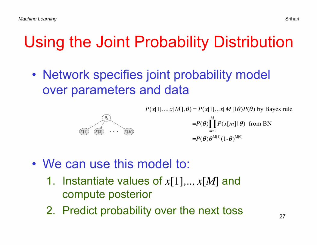
Using the Joint Probability Distribution

•  Network specifies joint probability model over parameters and data

•  We can use this model to: 1.  Instantiate values of x[1],.., x[M] and

compute posterior 2.  Predict probability over the next toss

27

qX

qX

X

Data m

(a) (b)

X [2]X [1] X [M]. . .

P(x[1],.., x[M ],θ ) = P(x[1],..x[M ] |θ )P(θ ) by Bayes rule

=P(θ ) P(x[m] |θ ) from m=1

M

∏ BN

=P(θ )θM[1](1-θ )M[0]


Computing A Parameter’s Posterior

1.  Determine posterior distribution of parameter •  From observed data set D instantiate values

x[1],..x[M] then compute posterior over θ

–  First term in numerator is likelihood –  Second is the prior–  Denominator is a normalizing factor –  If P(θ) is uniform, i.e., P(θ)=1 for all θ∈[0,1]

posterior is just the normalized likelihood function 28

P(θ | x[1],..x[M ]) = P(x[1].,, x[M ] |θ)P(θ)P(x[1],..x[M ])

P(θ |D ]) = P(D |θ)P(θ)P(D )

Machine Learning Srihari Prediction and Uniform Prior

•  For predicting probability of heads in next toss –  In Bayesian approach instead of single value for θ

we use its distribution •  Parameter is unknown, so we consider all

possible values, with D=x[1],.., x[M]

•  Integrating posterior over θ to predict prob heads in next toss

•  Thumbtack with Uniform Prior – Assume uniform prior over [0,1], i.e., P(θ)=1 – Substituting and P(D|θ)= θM[1](1-θ)M[0]

•  We get

P(x[M +1] | D) = P(x[M +1] |θ,D) P(θ | D)dθ∫ By Bayes rule & Sum rule

= P(x[M +1] |θ) P(θ | D)dθ∫ since samples are independent given θ

P(θ |D ]) = P(D |θ)P(θ)

P(D )

P(X[M +1] = x1 | D) = M[1]+1M[1]+ M[0]+ 2

Similar to MLE estimate except adds an imaginary sample to each count Called “Laplace’s Correction”

θ̂ =M[1]

M[1]+ M[0]

Machine Learning Srihari Non-uniform Prior

•  How to choose a non-uniform prior? •  Pick a distribution that can be represented

1.  Compactly, e.g., analytical formula 2.  Updated efficiently as we get new data

•  Appropriate prior is Beta Distribution –  Parameterized by two hyper-parameters

•  α0 and α1 which are positive reals •  They are imaginary numbers of heads and tails

we have seen before starting the experiment

30


Details of Beta Distribution •  Defined as

•  γ is a normalizing constant, defined as

•  Gamma function is a continuous generalization of factorials

•  Hyper-parameters correspond to no of heads and tails before experiment 31

θ ~ Beta(α1,α0 ) if p(θ) = γθα1 −1(1−θ)α0 −1

γ =Γ(α1 +α0 )Γ(α1)Γ(α0 )

where Γ(x)= t x−1e− t dt0

∞

∫ is the Gamma function

Γ(1) = 1 and Γ(x +1) = xΓ(x)Thus Γ(n +1) = n! when n is large


Examples of Beta Distribution For different hyperparameters

0 0.2 0.4 0.6 0.8 1q

p(q)

Beta (1,1)

0 0.2 0.4 0.6 0.8 1q

p(q)

Beta (10,10)

0 0.2 0.4 0.6 0.8 1q

p(q)Beta (2,2)

0 0.2 0.4 0.6 0.8 1q

p(q)

Beta (3,2)

0 0.2 0.4 0.6 0.8 1q

p(q)

0 0.2 0.4 0.6 0.8 1q

p(q)

Beta (15,10) Beta (0.5,0.5)

32

Machine Learning Srihari Thumbtack with Beta Prior

•  Marginal probability of X based on P(θ)~Beta(α0 , α1 )

33

P(X[1] = x1) = P(X[1] = x1 |θ )0

1

∫ ⋅P(θ )dθ= θ0

1

∫ ⋅P(θ )dθ =α 1

α 1 +α0

Using standard integration techniques Supports intuition that we have seen α1 heads and α0 tails What happens when we het more samples

P(θ |D ])∝ P(D |θ)P(θ) = θα1 +M [1]−1(1−θ)α0 +M [0]−1

Which is precisely Beta(α1+M[1],α0+M[0])

•  Key property of Beta distribution • If prior is a beta distribution, then posterior is also a beta distribution

• Beta is conjugate with Bernoulli • Immediate consequence is prediction (computing probability over next toss):

P(X[M +1] = x1 | D) = M[1]+α1M[1]+ M[0]+α1 +α0

Compare with uniform prior P(X[M +1] = x1 | D) = M[1]+1M[1]+ M[0]+ 2

Tells us that we have seen α1 +M[1] heads and α0+M[0] tails

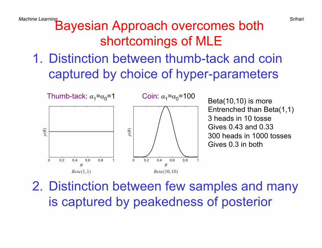
Machine Learning Srihari Bayesian Approach overcomes both

shortcomings of MLE 1.  Distinction between thumb-tack and coin

captured by choice of hyper-parameters

2.  Distinction between few samples and many

is captured by peakedness of posterior

0 0.2 0.4 0.6 0.8 1q

p(q)

Beta (1,1)

0 0.2 0.4 0.6 0.8 1q

p(q)

Beta (10,10)

0 0.2 0.4 0.6 0.8 1q

p(q)

Beta (2,2)

0 0.2 0.4 0.6 0.8 1q

p(q)

Beta (3,2)

0 0.2 0.4 0.6 0.8 1q

p(q)

0 0.2 0.4 0.6 0.8 1q

p(q)

Beta (15,10) Beta (0.5,0.5)

0 0.2 0.4 0.6 0.8 1q

p(q)

Beta (1,1)

0 0.2 0.4 0.6 0.8 1q

p(q)

Beta (10,10)

0 0.2 0.4 0.6 0.8 1q

p(q)

Beta (2,2)

0 0.2 0.4 0.6 0.8 1q

p(q)

Beta (3,2)

0 0.2 0.4 0.6 0.8 1q

p(q)

0 0.2 0.4 0.6 0.8 1q

p(q)

Beta (15,10) Beta (0.5,0.5)

Coin: α1=α0=100 Thumb-tack: α1=α0=1 Beta(10,10) is more Entrenched than Beta(1,1) 3 heads in 10 tosse Gives 0.43 and 0.33 300 heads in 1000 tosses Gives 0.3 in both


Multinomial Case: Bayesian Approach

•  Likelihood function (probability of iid samples)

L(θ:D)=∏kθkM[k]

•  Multinom. Distribn •  X takes one of K values x1..xK

•  θ ∈[0,1]K i.e, K reals in [0,1]

•  P(x:θ)=θk if x=xk

θ ~ Dirichlet(α1,..,α k ) if P(θ)∝k∏ θk

αk −1

•  Since posterior = prior x likelihood•  Require prior to have form similar to likelihood •  Dirichlet has that form

α = α jj∑


Dirichlet Distribution

•  Generalizes the Beta Distribution •  Specified by a set of hyper-parameters •  If P(θ) is Dirichlet(α1,..αK) then 1.  P(θ|D) is Dirichlet(α1+M[1],..,αK+M[K]) 2.  E[θk]=αk/α

36


Prediction with Dirichlet Prior

•  If posterior P(θ|D) is Dirichlet (α1+M[1],..,αK+M[K])

•  Prediction is

– Dirichlet hyper-parameters are called pseudocounts •  The total α of the pseudo counts reflects how

confident we are in our prior – Called the equivalent sample size

37

P(x[M +1] = xk |D) = M[k]+α k

M +α


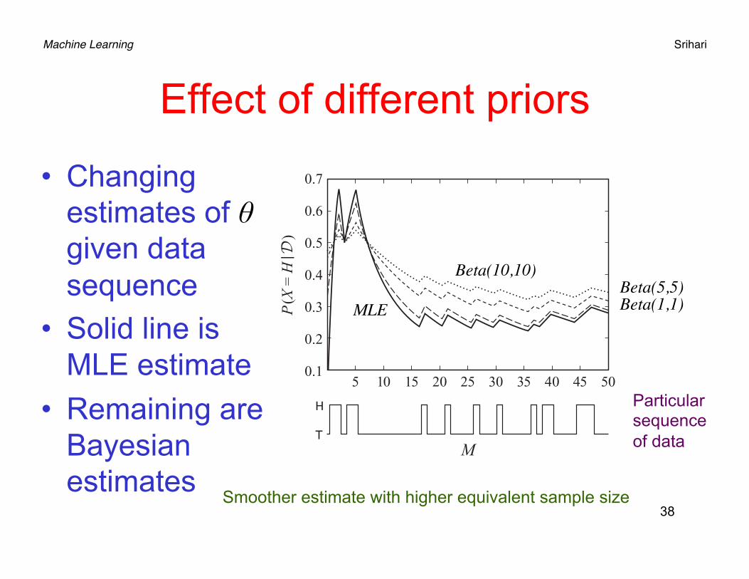
Effect of different priors

38

•  Changing estimates of θ given data sequence

•  Solid line is MLE estimate

•  Remaining are Bayesian estimates

0.7

0.6

0.5

0.4

0.3

0.2

0.1

M

505 10 15 20 25 30 35 40 45

T

H

P(X

= H

| )

Beta(10,10)

Beta(1,1)Beta(5,5)

MLE

Particular sequence of data

Smoother estimate with higher equivalent sample size


Dirichlet Process is about determining cardinality

•  A Dirichlet Process is an application of Dirichlet prior to a partial data problem

•  Problem of latent variables with unknown cardinality

•  A Bayesian approach is used over cardinalities •  A Dirichlet prior over K cardinalities is assumed •  Since K can be infinite, a legal prior is obtained

by defining a Chinese restaurant process 39

parameter estimation for bayesian networkssrihari/cse674/chap17/17.1-bn...• parameter values with...

Documents