introduction to likelihood what is covariance-based sem ...samples per estimated parameter –prefer...

2/10/19

1

Introduction to Likelihood Methods for SEM

Jarrett E. K. ByrnesUniversity of Massachusetts Boston

S =S(Q)

What is Covariance-Based SEM Estimation with Likelihood?

• Estimation of parameters given covariance of the data

• Equivalent to Linear Regressions, but…

• Estimation of each parameter influences the others

• Can accomodate unobserved (latent) variables and feedbacks

A Likely Outline

1. What SEM using likelihood and covariance matrices?

2. Model Identifiability

3. Sample Size for SEM

4. Introduction to lavaan

Maximizing Likelihood with One Parameter

Iteration over possible values simple

2/10/19

2

Likelihood with Two Parameters

• Algorithms used to search parameter space• Integrate answer over all data points – difficult computationally!

How does ML Estimation Work?

x1

y1

y2

Hypothesized Model Observed Covariance Matrix

{ 1.3.24 .41.01 9.7 12.3}S =

compareEvaluate Model Fit

+

ParameterEstimates

estimation

(e.g., maximum likelihood)

Σ = { σ11σ12 σ22σ13 σ23 σ33

}Implied Covariance Matrix

^

What we’re used to with ML

Data Generation: µi = a + bXi

Likelihood Function: Fr = Yi ~ dnorm(µi, s)

We minimize the likelihood function, Fr

It’s…More Complicated with SEM

Data Generation:

Likelihood Function:

FML = log Σ̂ − log S + tr SΣ̂−1( )− p+ q( )

2/10/19

3

The Maximum Likelihood Fitting Function

FML = log Σ̂ − log S + tr SΣ̂−1( )− p+ q( )

• If S =S, term 1 - 2 = 0 and terms 3 - 4 = 0. • FML = 0 with perfect fit

S = Sample covariance matrixS = Fit covariance matrixp = endogenous variablesq = exogenous variables

Linear Algebra Review

Det(A) = scalar number

A*A-1 = Diagonal matrix of ones

Assumptions Behind Fml• Multivariate normality

– Fairly robust (non-normality of residuals bigger problem)– Test with multivariate Shapiro-Wilk's Test (library mvnormtest)– In particular, no skew– Severe violations bias parameter error and tests of model fit

• No missing data in calculation of S– Biases your estimates with pairwise corrections

• No redundant variables– S must be positive definite

• Sample size is “large” (more soon)

A Likely Outline

1. What is different about fitting using likelihood and covariance matrices?

2. Identifiability

3. Sample Size (for likelihood and piecewise approaches)


Identifiability1.To fit a model, it must be identified

2.We need as much unique information as parameters

3.What can make a model non-identified?• Too many paths relative to # of variables• Certain model structures• High multicollinearity (r>0.9)• Complex model & small sample

4.How do I know if my model is identified?

2/10/19

4

Whither the T-Rule# of Parameters v. Covariance Matrix

• # Parameters £ # Unique Entries in a Covariance Matrix

T-rule: t £ (p+q)(p+q+1)/2

• t=# params, p = # endogenous variables, q = # exogenous variables

x1

y1

y2

z2

z1b12

g12 x1 y1 y2

x1 0.5

y1 0.7 0.5

y2 0.2 0.8 0.3

Cov(x,y1,y2)=

δ2

How Do I Count the Number of Parameters?

x1

y1

y2

z2

z1b12

g12

Yes, there is a variance here

If variance and covariances among exogenous variables is not shown either draw them or use modified formula:

T-rule: t* £ (p+q)(p+q+1)/2 - q(q+1)/2

You will see path diagrams drawn many ways…

Check what researcher is doing with exogenous variables!DF of all of these models = 4*5/2 – 8 = 2

x2

y1

y2

z2

z1

x1 x2

y1

y2

z2

z1

x1x2

y1

y2

z2

z1

x1

δ2δ1

Model Degrees of FreedomDF = tmax - t

Estimating 5 parameters from 6 variance/covariance relationships

DF=1Model Is Overidentified

x1

y1

y2

z2

z1b12

g12 x1 y1 y2

x1 0.5

y1 0.7 0.5

y2 0.2 0.8 0.3

Cov(x,y1,y2)=

2/10/19

5

Identification in SEM# of Parameters v. Covariance Matrix

x1

y1

y2

z2

z1b12

g12

Overidentified Just Identified

x1

y1

y2

z2

z1b12

g11

g12

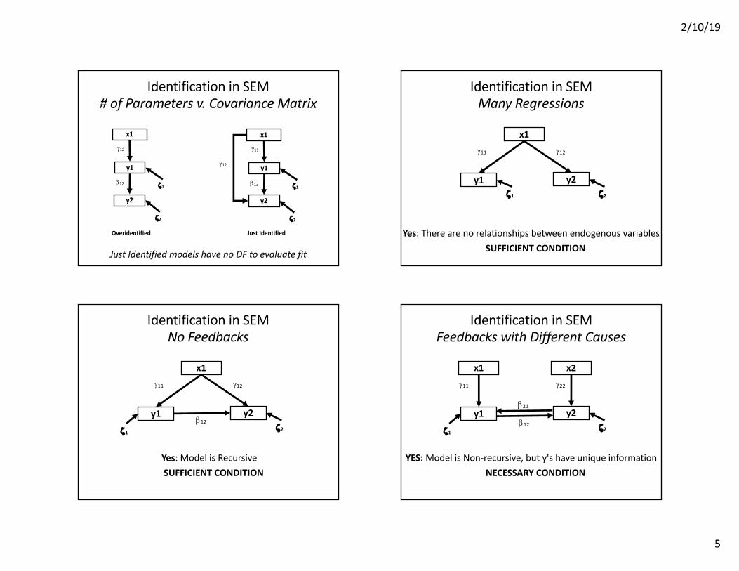
Just Identified models have no DF to evaluate fit

Identification in SEMMany Regressions

x1

y1 y2z2z1

g12g11

Yes: There are no relationships between endogenous variablesSUFFICIENT CONDITION

Identification in SEMNo Feedbacks

x1

y1 y2z2z1

g12g11

Yes: Model is RecursiveSUFFICIENT CONDITION

b12

Identification in SEMFeedbacks with Different Causes

x1

y1 y2z2z1

g22g11

YES: Model is Non-recursive, but y's have unique informationNECESSARY CONDITION

b12

b21

x2

2/10/19

6

Identification in SEMIs this model identified?

x1

y1 y2z2z1

g22g11

b12

b21

x2

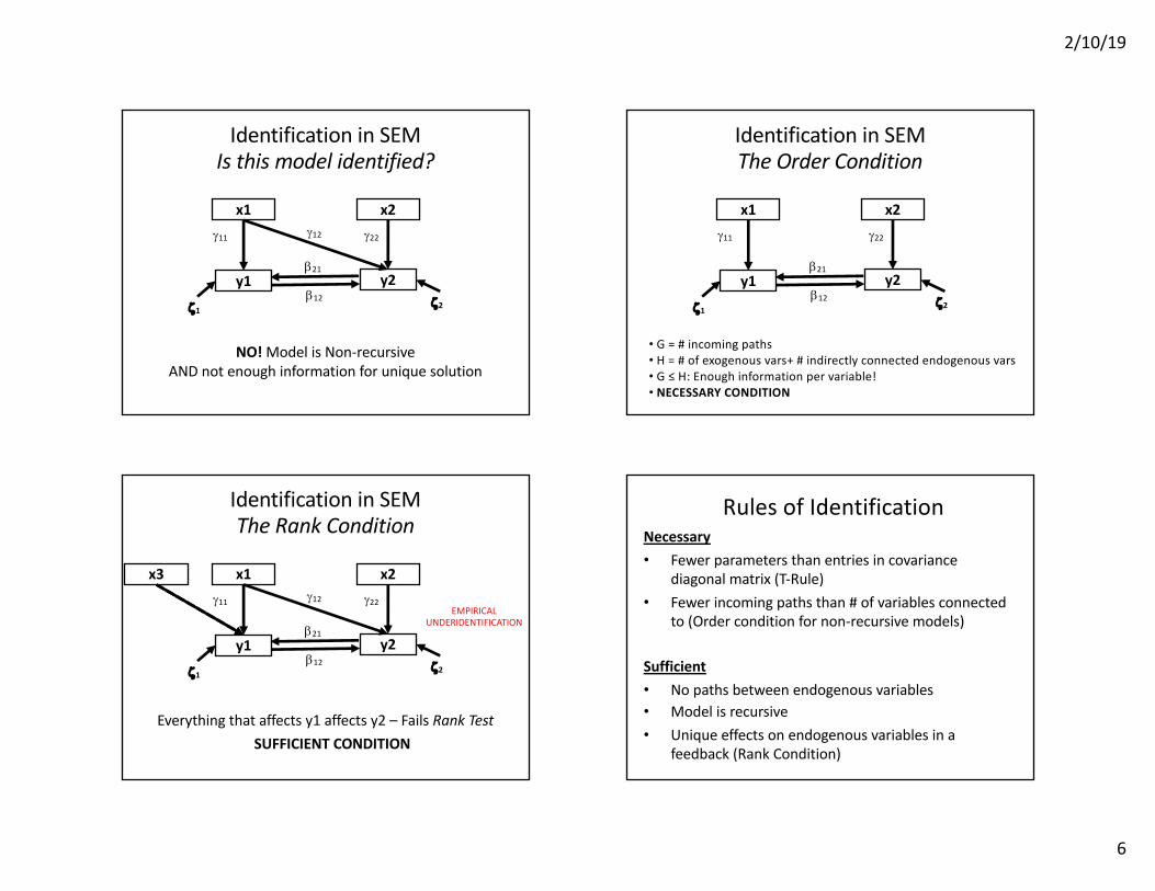
NO! Model is Non-recursiveAND not enough information for unique solution

g12

Identification in SEMThe Order Condition

x1

y1 y2z2z1

g22g11

b12

b21

x2

• G = # incoming paths• H = # of exogenous vars+ # indirectly connected endogenous vars• G ≤ H: Enough information per variable!• NECESSARY CONDITION

Identification in SEMThe Rank Condition

x1

y1 y2z2z1

g22g11

b12

b21

x2

Everything that affects y1 affects y2 – Fails Rank Test

g12

x3

SUFFICIENT CONDITION

EMPIRICALUNDERIDENTIFICATION

Rules of IdentificationNecessary• Fewer parameters than entries in covariance

diagonal matrix (T-Rule)• Fewer incoming paths than # of variables connected

to (Order condition for non-recursive models)

Sufficient• No paths between endogenous variables• Model is recursive• Unique effects on endogenous variables in a

feedback (Rank Condition)

2/10/19

7

A Likely Outline


2. Identifiability

3. Sample Size


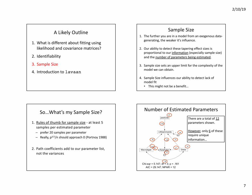
1. The further you are in a model from an exogenous data-generating, the weaker it's influence.

2. Our ability to detect these tapering effect sizes is proportional to our information (especially sample size) and the number of parameters being estimated.

3. Sample size sets an upper limit for the complexity of the model we can obtain.

4. Sample Size influences our ability to detect lack of model fit• This might not be a benefit…

Sample Size

So…What’s my Sample Size?

1. Rules of thumb for sample size - at least 5 samples per estimated parameter– prefer 20 samples per parameter– Really, p3/2/n should approach 0 (Portnoy 1988)

2. Path coefficients add to our parameter list, not the variances

There are a total of 12parameters shown.

However, only 6 of these require unique information…

Epiphytes

.41

Grass3.43

Macroalgae

LNGammarids

.19

ech

1

.44

egm

1

.37

-.16

.30 -.40 .31

.07

.24

pesticide

Chi-sqr = 5.147; df = 3; p = .161AIC = 29.147; NPAR = 12

-2.05

Number of Estimated Parameters

2/10/19

8

.59

Epiphytes GrassMacroalgae

.75

LNGammarids

ech

egm

.35

-.14

.42 -.79 .15

.18

pesticide

Chi-sqr = 5.147; df = 3; p = .161AIC = 29.147; NPAR = 12

-.75

29

Variances & covariance of exogenous variables can be obtained from the data. For “pesticide”, “Macroalgae”, and “Grass", this removes 4 parameters.

Error variances (and R2) for endogenous variables are calculated from other parameters. This removes 2 parameters.

Only 6 parameters require unique information. Samples/parameters = 40/6 = 6.7.

Parameters Needing Unique Information A Likely Outline


2. Identifiability

3. Sample Size (for likelihood and piecewise approaches)


What is lavaan?

• Stands for LAtent VAriable Analaysis

• Written by Yves Roseel in 2010

• Currently in version 5, but 6 coming soon

• Uses R lm syntax

1. SOFTWARE IS A TOOL

2. IT IS NOT PERFECT

3. ALWAYS MAKE SURE IT IS DOING WHAT YOU THINK IT IS DOING!

A Reminder

2/10/19

9

33

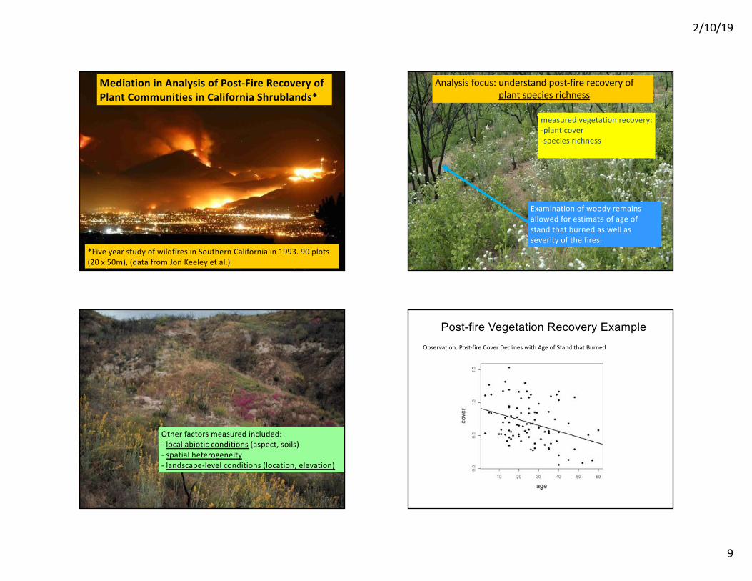
Mediation in Analysis of Post-Fire Recovery of Plant Communities in California Shrublands*

*Five year study of wildfires in Southern California in 1993. 90 plots (20 x 50m), (data from Jon Keeley et al.) 34

Analysis focus: understand post-fire recovery ofplant species richness

Examination of woody remains allowed for estimate of age of stand that burned as well as severity of the fires.

measured vegetation recovery:-plant cover-species richness

35

Other factors measured included:- local abiotic conditions (aspect, soils)- spatial heterogeneity- landscape-level conditions (location, elevation)

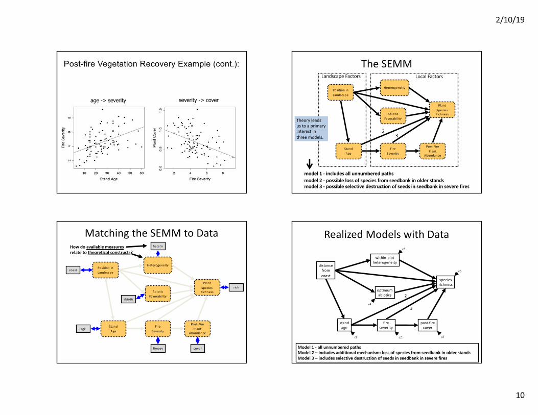
Post-fire Vegetation Recovery ExampleObservation: Post-fire Cover Declines with Age of Stand that Burned

2/10/19

10

Post-fire Vegetation Recovery Example (cont.):

age -> severity severity -> cover

38

2

Local FactorsLandscape Factors

Position inLandscape

AbioticFavorability

Post-FirePlant

Abundance

FireSeverity

StandAge

PlantSpecies

Richness

Heterogeneity

3

model 1 - includes all unnumbered pathsmodel 2 - possible loss of species from seedbank in older standsmodel 3 - possible selective destruction of seeds in seedbank in severe fires

Theory leads us to a primary interest in three models.

The SEMM

Position inLandscape

AbioticFavorability

Post-FirePlant

Abundance

FireSeverity

StandAge

PlantSpecies

Richness

Heterogeneity

age

coast

firesev cover

rich

hetero

abiotic

How do available measuresrelate to theoretical constructs?

Matching the SEMM to Data

40

standage

fireseverity

e2

post-firecover

e1 e3

distancefromcoast

optimumabiotics

within-plotheterogeneity

speciesrichness

e6

e5

e4

2

3

Model 1 - all unnumbered pathsModel 2 – includes additional mechanism: loss of species from seedbank in older standsModel 3 – includes selective destruction of seeds in seedbank in severe fires

Realized Models with Data

2/10/19

11

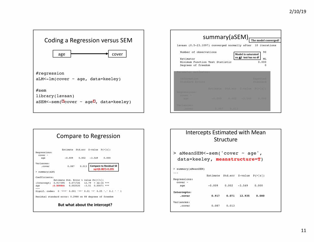
Coding a Regression versus SEM

#regressionaLM<-lm(cover ~ age, data=keeley)

#semlibrary(lavaan)aSEM<-sem('cover ~ age', data=keeley)

age cover

summary(aSEM)lavaan (0.5-23.1097) converged normally after 10 iterations

Number of observations 90

Estimator MLMinimum Function Test Statistic 0.000Degrees of freedom 0

Parameter estimates:

Information ExpectedStandard Errors Standard

Estimate Std.err Z-value P(>|z|)Regressions:cover ~age -0.009 0.002 -3.549 0.000

Variances:.cover 0.087 0.013

Modelissaturatedso,c2 test has no df

Themodelconverged!

Compare to Regression



> summary(aLM)

Coefficients:Estimate Std. Error t value Pr(>|t|)

(Intercept) 0.917395 0.071726 12.79 < 2e-16 ***age -0.008846 0.002520 -3.51 0.00071 ***---Signif. codes: 0 ‘***’ 0.001 ‘**’ 0.01 ‘*’ 0.05 ‘.’ 0.1 ‘ ’ 1

Residual standard error: 0.2988 on 88 degrees of freedom

Compare to Residual SEsqrt(0.087)=0.295

But what about the intercept?

Intercepts Estimated with Mean Structure

> aMeanSEM<-sem('cover ~ age', data=keeley, meanstructure=T)

> summary(aMeanSEM)...


Intercepts:.cover 0.917 0.071 12.935 0.000


2/10/19

12

Intercepts Estimated with Mean Structure

> aMeanSEM<-sem('cover ~ age', data=keeley, meanstructure=T)

age cover

1

Slope

Intercept

Standardized Coefficients>standardizedSolution(aSEM)

lhs op rhs est.std se z pvalue1 cover ~ age -0.350 0.090 -3.912 02 cover ~~ cover 0.877 0.063 13.973 03 age ~~ age 1.000 0.000 NA NA

age cover-0.35

0.88

Also: summary(aSEM, standardized=T, rsq=T)

Can I See It?library(lavaanPlot)lavaanPlot(model = aSEM, coefs = TRUE)

Can I See It?lavaanPlot(model = aSEM, coefs = TRUE,

stand=TRUE)

2/10/19

13

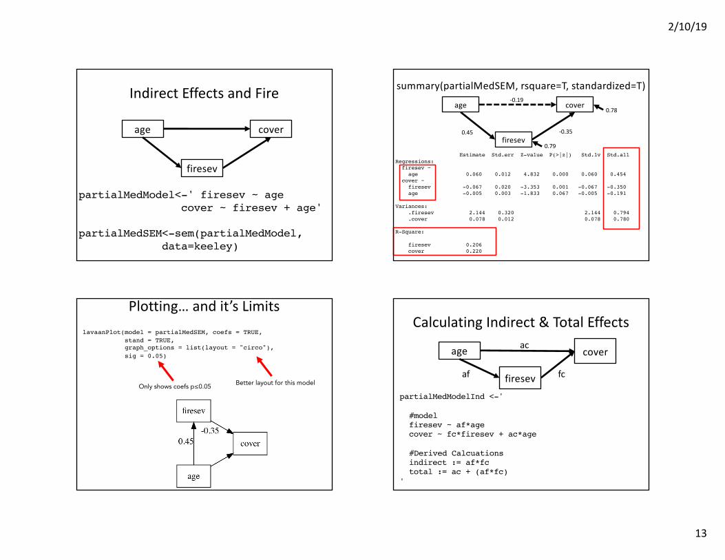
Indirect Effects and Fire

partialMedModel<-' firesev ~ agecover ~ firesev + age'

partialMedSEM<-sem(partialMedModel, data=keeley)

age cover

firesev

summary(partialMedSEM, rsquare=T, standardized=T)

Estimate Std.err Z-value P(>|z|) Std.lv Std.allRegressions:firesev ~age 0.060 0.012 4.832 0.000 0.060 0.454

cover ~firesev -0.067 0.020 -3.353 0.001 -0.067 -0.350age -0.005 0.003 -1.833 0.067 -0.005 -0.191

Variances:.firesev 2.144 0.320 2.144 0.794.cover 0.078 0.012 0.078 0.780

R-Square:

firesev 0.206cover 0.220

age cover

firesev0.45 -0.35

-0.190.78

0.79

Plotting… and it’s LimitslavaanPlot(model = partialMedSEM, coefs = TRUE,

stand = TRUE, graph_options = list(layout = "circo"),sig = 0.05)

Better layout for this modelOnly shows coefs p≤0.05

Calculating Indirect & Total Effects

partialMedModelInd <-'

#modelfiresev ~ af*agecover ~ fc*firesev + ac*age

#Derived Calcuationsindirect := af*fctotal := ac + (af*fc)

'

age cover

firesev

ac

af fc

2/10/19

14


Estimate Std.err Z-value P(>|z|)Regressions:firesev ~age (af) 0.060 0.012 4.832 0.000

cover ~firesev (fc) -0.067 0.020 -3.353 0.001age (ac) -0.005 0.003 -1.833 0.067

age cover

firesev

ac

af fc


Estimate Std.err Z-value P(>|z|)

...

Defined parameters:indirect -0.004 0.001 -2.755 0.006total -0.009 0.002 -3.549 0.000

age cover

firesev

ac

af fc


> standardizedSolution(partialMedSEMInd)lhs op rhs est.std se z pvalue

...10 indirect := af*fc -0.159 0.054 -2.947 0.00311 total := ac+(af*fc) -0.350 0.090 -3.912 0.000

age cover

firesev

ac

af fc

Take Lavaan for a Spin!1. Fit this model!2. Fill in Standardized Coefficients and R2 for

this model3. Calculate summed direct and indirect effects

of distance on richness4. Call out with warnings, errors, etc!

distance rich

hetero

abiotic

2/10/19

15

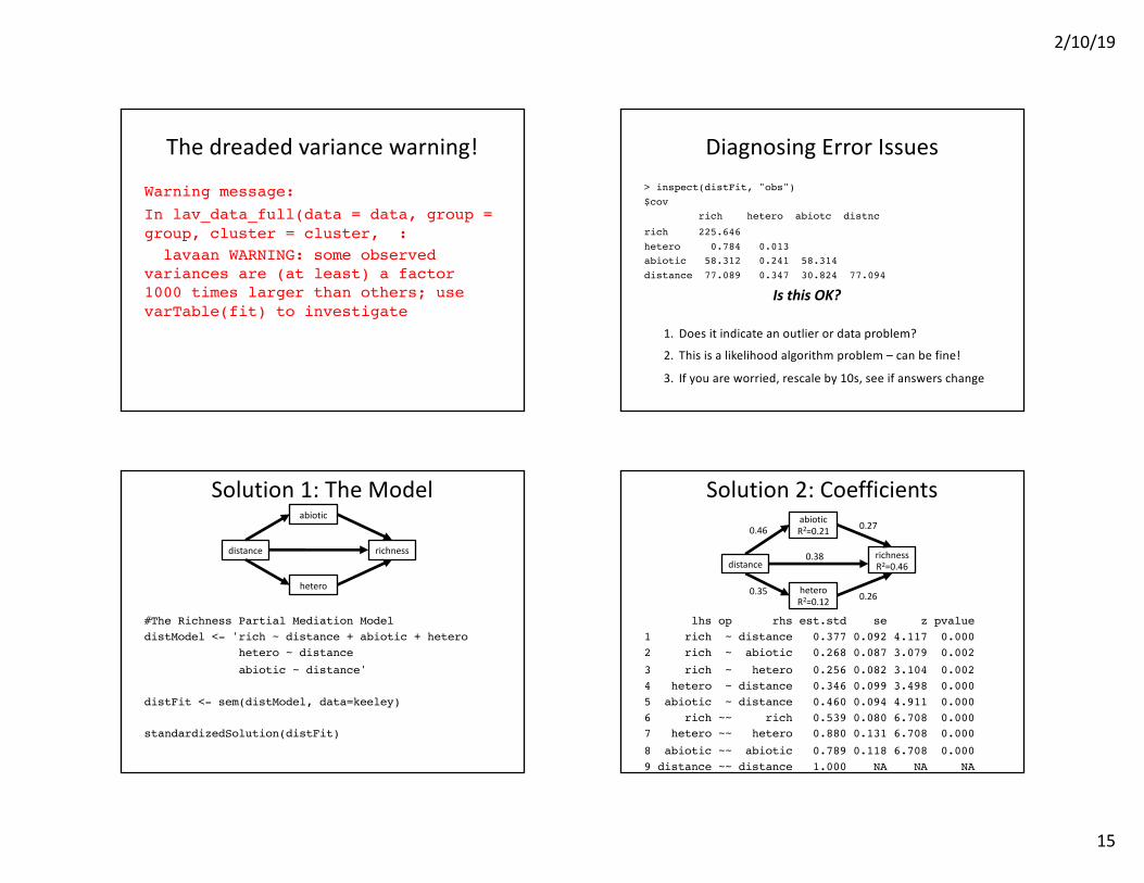
The dreaded variance warning!

Warning message:In lav_data_full(data = data, group = group, cluster = cluster, :lavaan WARNING: some observed

variances are (at least) a factor 1000 times larger than others; use varTable(fit) to investigate

Diagnosing Error Issues> inspect(distFit, "obs")$cov

rich hetero abiotc distnc rich 225.646 hetero 0.784 0.013 abiotic 58.312 0.241 58.314 distance 77.089 0.347 30.824 77.094

Is this OK?

1. Does it indicate an outlier or data problem?

2. This is a likelihood algorithm problem – can be fine!

3. If you are worried, rescale by 10s, see if answers change

Solution 1: The Model

#The Richness Partial Mediation ModeldistModel <- 'rich ~ distance + abiotic + hetero

hetero ~ distanceabiotic ~ distance'

distFit <- sem(distModel, data=keeley)

standardizedSolution(distFit)

distance richness

hetero

abiotic

Solution 2: Coefficients

lhs op rhs est.std se z pvalue1 rich ~ distance 0.377 0.092 4.117 0.0002 rich ~ abiotic 0.268 0.087 3.079 0.0023 rich ~ hetero 0.256 0.082 3.104 0.0024 hetero ~ distance 0.346 0.099 3.498 0.0005 abiotic ~ distance 0.460 0.094 4.911 0.0006 rich ~~ rich 0.539 0.080 6.708 0.0007 hetero ~~ hetero 0.880 0.131 6.708 0.0008 abiotic ~~ abiotic 0.789 0.118 6.708 0.0009 distance ~~ distance 1.000 NA NA NA

distancerichnessR2=0.46

heteroR2=0.12

abioticR2=0.21

0.38

0.27

0.260.35

0.46

2/10/19

16

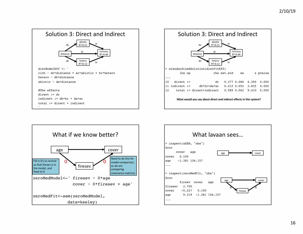
Solution 3: Direct and Indirect

distModelEff <- 'rich ~ dr*distance + ar*abiotic + hr*heterohetero ~ dh*distanceabiotic ~ da*distance

#The effectsdirect := drindirect := dh*hr + da*artotal := direct + indirect'


heteroR2=0.12

abioticR2=0.21

dr

ar

hrdh

da

Solution 3: Direct and Indirect

> standardizedSolution(distFitEff)lhs op rhs est.std se z pvalue

...10 direct := dr 0.377 0.086 4.390 0.00011 indirect := dh*hr+da*ar 0.212 0.055 3.835 0.00012 total := direct+indirect 0.589 0.062 9.433 0.000


heteroR2=0.12

abioticR2=0.21

dr

ar

hrdh

da

What would you say about direct and indirect effects in this system?

What if we know better?

zeroMedModel<-' firesev ~ 0*agecover ~ 0*firesev + age'

zeroMedFit<-sem(zeroMedModel, data=keeley)

age cover

firesev00Fill in 0's to remind

us that firesev is in the model, and fixed to 0

Need to do this for model comparison, as we are comparing covariance matrices

What lavaan sees…> inspect(aSEM, "obs")$cov

cover age cover 0.100 age -1.381 156.157...

> inspect(zeroMedFit, "obs")$cov

firesv cover age firesev 2.700 cover -0.227 0.100 age 9.319 -1.381 156.157...

age cover

firesev00

age cover

2/10/19

17

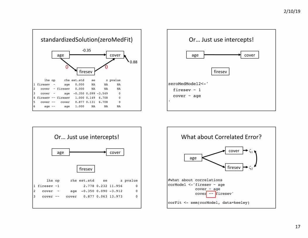
standardizedSolution(zeroMedFit)

lhs op rhs est.std se z pvalue1 firesev ~ age 0.000 NA NA NA2 cover ~ firesev 0.000 NA NA NA3 cover ~ age -0.350 0.099 -3.549 04 firesev ~~ firesev 1.000 0.149 6.708 05 cover ~~ cover 0.877 0.131 6.708 06 age ~~ age 1.000 NA NA NA

age cover

firesev00

-0.35

0.88

Or… Just use intercepts!

zeroMedModel2<-'firesev ~ 1cover ~ age

'

age cover

firesev

Or… Just use intercepts!

lhs op rhs est.std se z pvalue1 firesev ~1 2.778 0.232 11.956 02 cover ~ age -0.350 0.090 -3.912 03 cover ~~ cover 0.877 0.063 13.973 0

age cover

firesev

What about Correlated Error?

#what about correlationscorModel <-'firesev ~ age

cover ~ agecover ~~ firesev'

corFit <- sem(corModel, data=keeley)

agecover

firesev

z1

z2

2/10/19

18

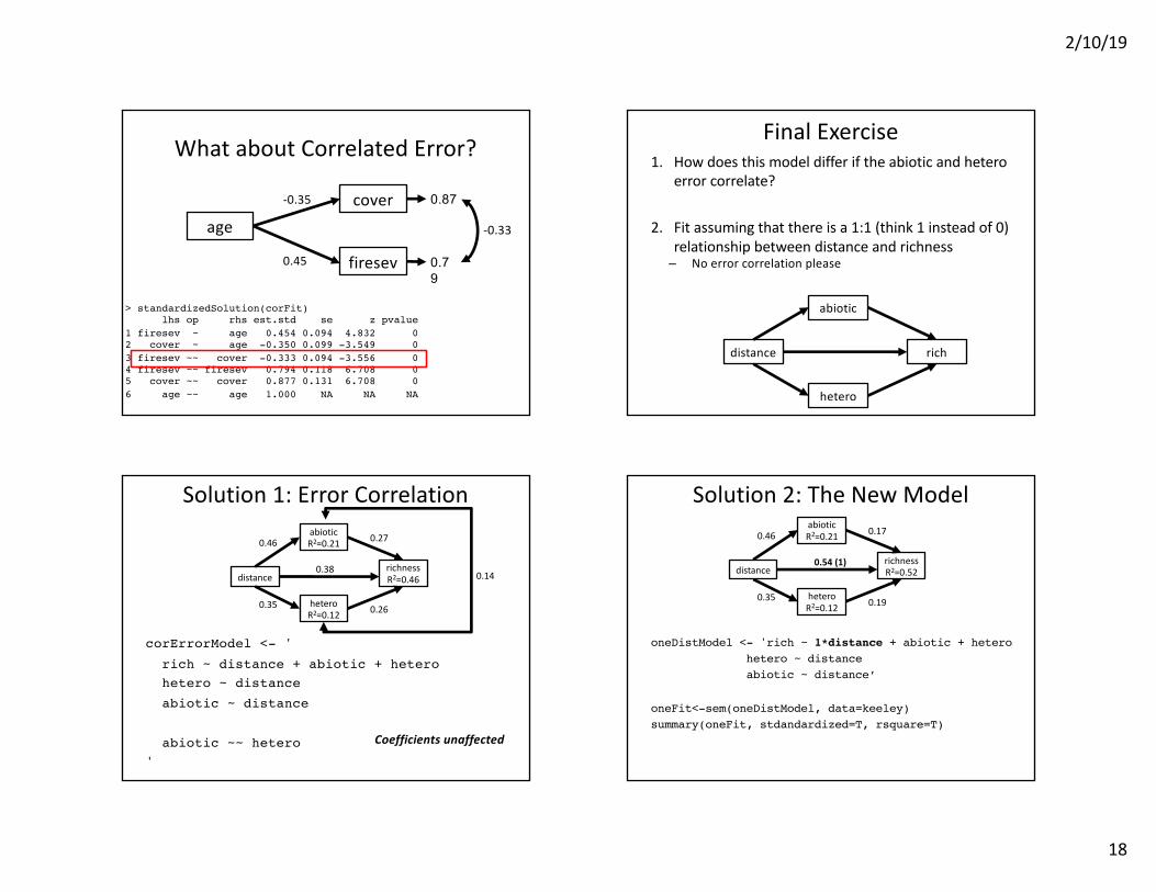
What about Correlated Error?

> standardizedSolution(corFit)lhs op rhs est.std se z pvalue

1 firesev ~ age 0.454 0.094 4.832 02 cover ~ age -0.350 0.099 -3.549 03 firesev ~~ cover -0.333 0.094 -3.556 04 firesev ~~ firesev 0.794 0.118 6.708 05 cover ~~ cover 0.877 0.131 6.708 06 age ~~ age 1.000 NA NA NA

agecover

firesev

0.87

0.79

-0.35

0.45

-0.33

Final Exercise1. How does this model differ if the abiotic and hetero

error correlate?

2. Fit assuming that there is a 1:1 (think 1 instead of 0) relationship between distance and richness – No error correlation please

distance rich

hetero

abiotic

Solution 1: Error Correlation

corErrorModel <- 'rich ~ distance + abiotic + heterohetero ~ distanceabiotic ~ distance

abiotic ~~ hetero'


heteroR2=0.12

abioticR2=0.21

0.38

0.27

0.260.35

0.46

0.14

Coefficients unaffected

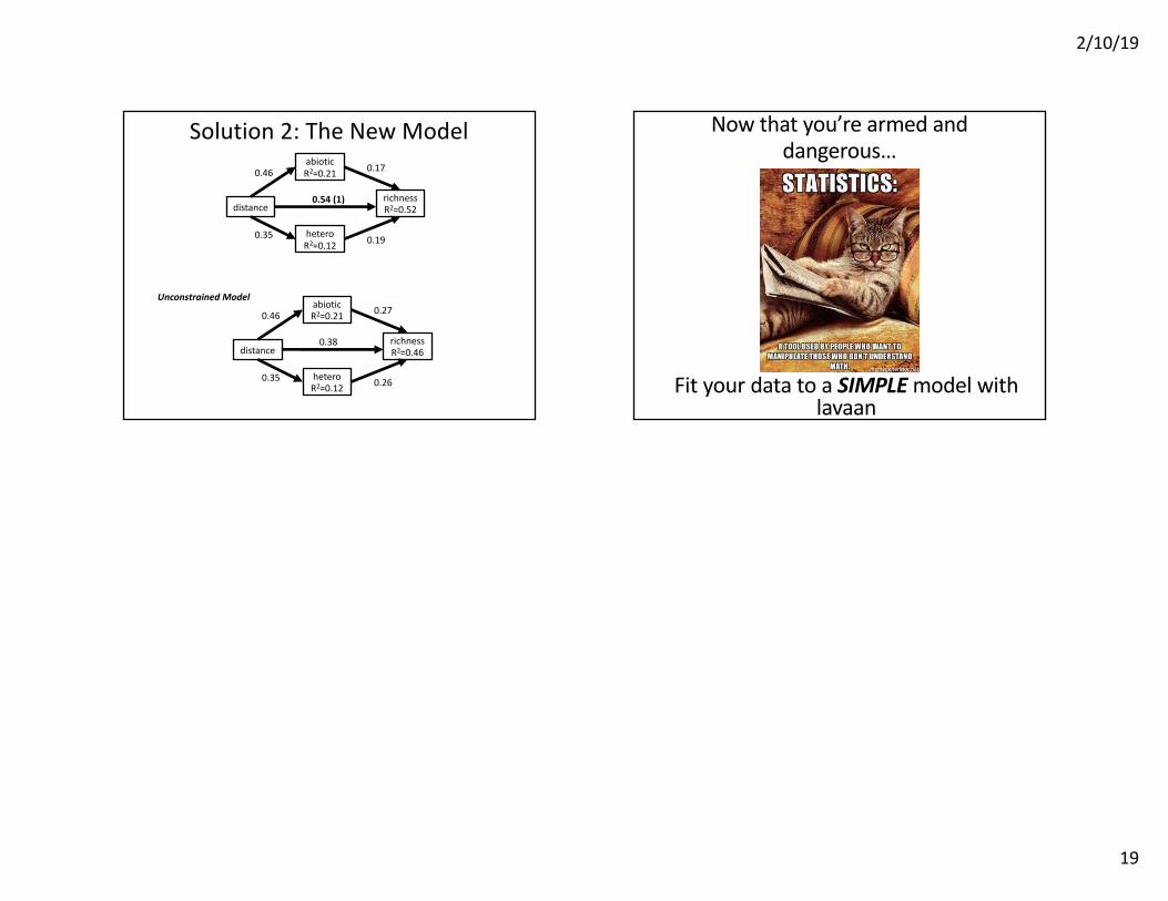
Solution 2: The New Model

oneDistModel <- 'rich ~ 1*distance + abiotic + heterohetero ~ distanceabiotic ~ distance’

oneFit<-sem(oneDistModel, data=keeley)summary(oneFit, stdandardized=T, rsquare=T)


heteroR2=0.12

abioticR2=0.21

0.54 (1)

0.17

0.190.35

0.46

2/10/19

19

Solution 2: The New Model


heteroR2=0.12

abioticR2=0.21

0.54 (1)

0.17

0.190.35

0.46


heteroR2=0.12

abioticR2=0.21

0.38

0.27

0.260.35

0.46

Unconstrained Model

Now that you’re armed and dangerous…

Fit your data to a SIMPLE model with lavaan

introduction to likelihood what is covariance-based sem ...samples per estimated parameter –prefer...

Documents