PARALLEL DISTRIBUTED PROCESSING

Explorations in the Microstructure of Cognition

Volume 1: Foundations

David E. Rumelhart James L. McClelland

and the PDP Research Group

Chisato Asanuma Alan H. Kawamoto Paul Smolensky Francis H. C . Crick Paul W. Munro Gregory 0. Stone Jeffrey L. Elman Donald A. Norman Ronald J . Williams Geoffrey E. Hinton Daniel E. Rabin David Zipser Michael I . Jordan Terrence J . Sejnowski

Institute for Cognitive Science University of California, San Diego

A Bradford Book

The MIT Press Cambridge, Massachusetts

London, England

0 1986 by. The Massachusetts Institute of Technology

All rights reserved. No part of this book may be reproduced in any form by any electronic or mechanical means (including photocopying, recording, or information storage and retrieval) without permission in writing from the publisher.

Printed and bound in the United States of America

Library of Congress Cataloging-in-Publication Data

Rumelhart, David E. Parallel distributed processing.

(Computational models of cognition and perception) Vol. 2 by James L. McClelland, David E. Rumelhart,

and the PDP Research Group. "A Bradford book." Includes bibliographies and indexes. Contents: v. 1. Foundations - v. 2. Psychological

and biological models. 1. Human information processing. 2. Cognition.

I. McClelland, James L. 11. University of California, San Diego. PDP Research Group. 111. Title. IV. Series. BF455.R853 1986 153 85-24073 ISBN 0-262-18120-7 (v. 1)

0-262- 132 18-4 (v. 2) 0-262- 18 123- 1 (set)

. . , . . . . . . . . . I . . . . . . . . . . . . . . . .

CHAPTER 7

Learning and Relearning in Boltzmann Machines

G. E. HINTON and T . J. SEJNOWSKI

Many of the chapters in this volume make use of the ability of a paral- lel network to perform cooperative searches for good solutions to prob- lems. The basic idea is simple: The weights on the connections between processing units encode knowledge about how things nornlally f i t together in some domain and the initial states or external inputs to a subset of the units encode some fragments of a structure within the domain. These fragments constitute a problem: What is the whole structure from which they probably came? The network computes a "good solution" to the problem by repeatedly updating the states of units that represent possible other parts of the structure until the net- work eventually settles into a stable state of activity that represents the solution.

One field in which this style of computation seems particularly appropriate is vision (Ballard, Hinton, & Sejnowski, 1983). A visual system must be able to solve large constraint-satisfaction problems rapidly in order to interpret a two-dimensional intensity image in terms of the depths and orientations of the three-dimensional surfaces in the world that gave rise to that image. In general, the information in the image is not sufficient to specify the three-dimensional surfaces unless the interpretive process makes use of additional plausible constraints about the kinds of structures that typically appear. Neighboring pieces of an image, for example, usually depict fragments of surface that have similar depths, similar surface orientations, and the same reflectance. The most plausible interpretation of an image is the one that satisfies

1 I constrai~its of this kind as well as possible, and the human visual sys- I ten1 stores enough plausible constraints and is good enough at applying

them that i r can arrive at the correct interpretation of most normal images.

The computation may be perl'orrnetl by a n iterative search which starts with a poor interprelation and progressively improves i t by reduc- ing a cost function that measures the extent to which the current interpretation violates the plausible constraints. Suppose, for example, that each un i t stands for a small three-dimensional surface fragment, and the state of the unit indicates the current bet about whether that surface fragment is part of the best three-dimensional interpretation. Plausible constraints about the nature of surfaces can then be encoded by the pairwise interactions between processing elements. For example, iwo units that stand Sor neighboring surface fragments of similar depth and surface orientation can be mutually excitatory to encode the constraints that each of these hypotheses tends to support the other (because objects tend to have continuous surfaces).

RELAXATION SEARCHES

The general idea of using parallel networks to perform relaxation searches that simultaneously satisf'y multiple constr~~ints is appealing. I t might even provide a successor to telephone exchanges, holograms, or con~n~unities of agents as a metaphor f'or the style of computation in cerebral cortex. But some tough technical questions have to be answered before this style of computation can be accepted as either efficient or plausible:

Will the network settle down or will it oscillate or wander aim- lessly?

What does the network compute by settling down? We need some characterization of the computation that the network per- forms other than the network itself. Ideally we would like to be able to say what ought to be computed (Marr, 1982) and then to show that a network can be made to compute i t .

How long does the network take to settle on a solution? If thousands of iterations are required the method becomes implausible as a model of how the cortex solves constraint- satisfaction problems.

How much information does each unit need to convey to its 'neighbors? In many relaxation schemes the units communicate accurate real values to one another on each iteration. Again this is implausible if the units are intended to be like cortical neurons which comn~unicate using all-or-none spikes. To send a real-value, accurate to within 5%, using firing rates requires about 100 ms which is about the time allowed for the whole iterative process to settle down.

How are the weights that encode the knowledge acquired? For models of low-level vision i t is possible for a programmer to decide on the weights, and evolution might do the same for the earliest stages of biological visual systems. But if the same kind of constraint-satisfaction searches are to be used for higher level functions like shape recognition or content-addressable memory, there must be some learning procedure that autornati- cally encodes properties of the domain into the weights.

This chapter is mainly concerned with the last of these questions, b u ~ the learning procedure we present is an unexpected consequence of our attempt to answer the other questions, so we shall start with them.

Relaxation, Optimization, and Weak Constraints

One way of ensuring that a relaxation search is computing something sensible (and will eventually settle down) is to show that i t is solving an optimization problem by progressively reducing the value of a cost function. Each possible state of activity of the network has an associ- ated cost, and the rule used for updating activity levels is chosen so that this cost keeps falling. The cost function must be chosen so that low-cost states represent good solutions to problems in the domain.

Many optimization problems can be cast in a framework known as linear programming. There are some variables which take on real values and there are linear equality and inequality constraints bet ween variables. Each combination of values for the variables has an associ- ated cost which is the sum over all the variables of the current value times a cost-coefficient. The aim is to find a combination of values that satisfies all the constraints and minimizes the cost function. If the variables are further constrained to take on only the values 1 or 0 the problem is called zero-one programming. Hinton (1977) has shown that certain zero-one programming problems can be implemented as relaxation searches in parallel networks. This allows networks to find

7 L E A R N I N G IN I 3 0 L T Z M A N N MACf1INES 285

good solutions to problems in which there are discrete hypotheses that are true or false. Even though the allowable so lu t~ons all assign values of 1 or 0 to the hypotheses, the relaxation process works by passing through intermediate states in which hypothesis units have real-valued act~vity levels lying between 1 and 0. Each constraint is enforced by a feedback loop that measures the amount by which the current values violate the constraint and tries to alter the values of the variables to reduce this violation.

Linear programming and its variants make a sharp distinction between constraints (which must be satisfied) and costs. A solution which achieves a very low cost by violating one or two of the con- straints is simply not allowed. In many domains, the distinction between constraints and costs is not so clear-cut. In vision, for example, i t is usually helpful to use the constraint that neighboring pieces of surface are at similar depths because surfaces are mostly con- t ~ n u o u s and are rarely parallel to the line of sight. But this is not an absolute constraint. I t doesn't apply at the edge of an object. So a visual system needs to be able to generate interpretations that violate this constraint if i t can satisfy many other constraints by doing so. Constraints like these have been called "weak" constraints (Blake, 1983) and ~t is possible to formulate optimization problems In which all the constraints are weak and there is no distinction between constraints and costs. The optimal solution is then the one wh~ch m i n ~ m ~ z e s the total constraint violation where different constraints are glven different strengths depending on how reliable they are. Another way of saying this is that all the constraints have associated plaus~bilities, and the most plausible solution is the one which fits these plausible constraints as well as possible.

Some relaxation schemes dispense with separate feedback loops for the constraints and implement weak constraints directly in the excita- tory and inhibitory interactions between units. We would like these networks to settle into states in which a few units are fully active and the rest are inactive. Such states constitute clean "digital" interpreta- tions. To prevent the network from hedging its bets by settling into a state where many units are slightly active, i t is usually necessary to use a strongly nonlinear decision rule, and this also speeds convergence. However, the strong nonlinearities that are needed to force the network to make a decision also cause it to converge on different states on dif- ferent occasions: Even with the same external inputs, the final state depends on the initial state of the net. This has led many people (Hop- field, 1982; Rosenfeld, Hummel, & Zucker, 1976) to assume that the particular problem to be solved should be encoded by the initial state of the network rather than by sustained external input to some of its units.

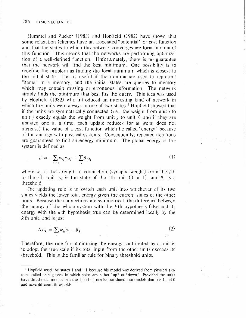
Hummel and Zucker (1983) and Hopfield (1982) have shown that some relaxation Schemes have an associated "potential" or cost function and that the states to which the network converges are local minima of this function. This means that the networks are performing optiniiza- tion of a well-defined function. Unfortunately, there is no guarantee that the network will find the best minimum. One possibility is to redefine the problem as finding the local minimum which is closest to the initial state. This is useful if the minima are used to represent "items" in a memory, and the initial states are queries to memory which may contain missing or erroneous information. The network simply finds the minimum that best fits the query. This idea was used by Hopfield (1982) who introduced an interesting kind of network in which the units were always in one of two states. ' Hopfield showed that if the units are syn~metrically connected (i.e., the weight from unit i to unit j exactly equals the weight from unit j to unit i) and if they are updated one at a time, each update reduces (or at worst does not increase) the value of a cost function which he called "energy" because of the analogy with physical systems. Consequently, repeated iterations are guaranteed to find an energy minimum. T h e global energy of the system is defined as

where w,, is the strength of connection (synaptic weight) from the , j th to the i th unit, s, is the state of the i t h unit (0 or l ) , and 0 , is a threshold.

T h e updating rule is to switch each unit into whichever of its two states yields the lower total energy given the current states of the other units. Because the connections are symmetrical, the difference between the energy of the whole system with the k t h hypothesis false and its energy with the k th hypothesis t rue can be determined locally by the k t h unit, and is just

Therefore, the rule for minimizing the energy contributed by a unit is to adopt the true state if its total input f rom the other units exceeds its threshold. This is the familiar rule for binary threshold units.

I Hopfield used the states 1 and - 1 because his model was derived from physical sys- tems called spin glasses in which spins are either "up" or "down." Provided the units have thresholds, models that use 1 and - 1 can be translated into models that use 1 and 0 and have different thresholds.

7 L E A R N I N G IN BOLTZMANN MACHINES 287

) Using Probabi l is t ic Dec i s ions t o Escape F r o m Local Min ima

1 At about the same t ime that Hopfield showed how parallel networks of this kind could be used to access memories that were stored as local minima, Kirkpatrick, working at IBM, introduced an interesting new

i search technique for solving hard optimization problems on conven- tional computers.

One standard technique is to use gradient descent: The values of the variables in the problem are modified in whatever direction reduces the cost function (energy). For hard problems, gradient descent gets stuck at local minima that a re not globally optimal. This is an inevitable consequence of only allowing downhill moves. If jumps to higher energy states occasionally occur, i t is possible to break out of local minima, but i t is not obvious how the system will then behave and i t is far from clear when uphill steps should be allowed.

Kirkpatrick, Gelatt, and Vecchi (1983) used another physical analogy to guide the use of occasional uphill steps. T o find a very low energy state of a metal, t he best strategy is to melt it and then to slowly reduce its temperature. This process is called annealing, and so they named their search method "simulated annealing." Chapter 6 contains a dis- cussion of why annealing works. W e give a simple intuitive account here.

One way of seeing why thermal noise is helpful is to consider the energy landscape shown in Fig~lre 1 . Let us suppose thar a ball-bearing starts at a randomly chosen point on the landscape. I f i t always goes downhill (and has no inertia), i t will have an even chance of ending up at A or B because both minima have the same width and so the initial

FIGURE 1. A simple energy landscape containing two local nimrna separated by a n energy barrier. Shaking can be used to allow the state of the network (represented here by a ball-bearing) to escape from local minima.

random point is equally likely to lie in either minimum. If we shake the .whole system, we are more likely to shake the ball-bearing from A to B than vice versa because the energy barrier is lower from the A side. If the shaking is gentle, a transition from A to B will be many times as probable as a transition from B to A, but both transitions will be very rare. So although gentle shaking will ultimately lead to a very high probability of being in B rather than A, it will take a very long time before this happens. On the other hand, if the shaking is violent, the ball-bearing will cross the barrier frequently and so the ultimate probability ratio will be approached rapidly, but this ratio will not be very good: With violent shaking i t is almost as easy to cross the barrier in the wrong direction (from B to A) as in the right direction. A good compromise is to start by shaking hard and gradually shake more and more gently. This ensures that at some stage the noise level passes through the best possible compromise between the absolute probability of a transition and the ratio of the probabilities of good and bad transi- tions. I t also means that at the end, the ball-bearing stays right at the bottom of the chosen minimum.

This view of why annealing helps is not the whole story. Figure 1 is misleading because all the states have been laid out in one dimension. Complex systems have high-dimensional state spaces, and so the barrier between two low-lying states is typically massively degenerate: The number of ways of getting from one low-lying state to another is an exponential function of the height of the barrier one is willing to cross. This means that a rise in the level of thermal noise opens u p an enor- mous variety of paths for escaping from a local minimum and even though each path by itself is unlikely, i t is highly probable that the sys- tem will cross the barrier. We conjecture that simulated annealing will only work well in domains where the energy barriers are highly degenerate.

Applying Simulated Annealing to Hopfield Nets

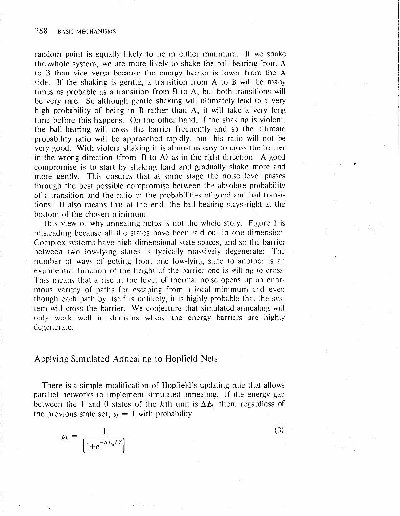
There is a simple modification of Hopfield's updating rule that allows parallel networks to implement simulated annealing. If the energy gap between the 1 and 0 states of the k t h unit is AEk then, regardless of the previous state set, sk = 1 with probability

where T is a parameter which acts like the temperature of a physical system. This local decision rule ensures that in thermal equilibrium the relative probability of two global states is deterniined solely by their energy difference, and follows a Boltzmann distribution:

where P, is the probability of being in the a t h global state, and E,, is the energy of that state.

At low temperatures there is a strong bias in favor of states with low energy, but t he t ime required to reach equilibrium may be long. At higher temperatures the bias is not so favorable, but equilibrium is reached faster. T h e fastest way to reach equilibrium at a given tem- perature is generally to use simhlated annealing: Start with a higher temperature and gradually reduce it.

T h e idea of implementing constraints as interactions between sto- chastic processing elements was proposed by Moussouris (1 974) who discussed the identity between Boltzniann d~srributions and Markov random fields. T h e idea of using simulated annealing to find low energy states in parallel networks has been investigated independently by several different groups. S. Genian and D. Geman (1984) esta- blished limits on the allowable speed of the annea l~ng schedule and showed that siniulated annealing can be very efl'ect~ve for removing noise from images. Hinton and Sejnowski (1983b) showed how the use of binary stochastic elements could solve some problems that plague other relaxation techniques, in particular the problem of learning the weights. Smolensky ( 1 983) has been investigating a similar scheme which h e calls "harmony theory." This scheme is discussed in detail in Chapter 6. Smolensky's harmony is equivalent to our energy (with a sign reversal).

Pattern Completion

One way of using a parallel network is to treat it as a pattern comple- tion device. A subset of the units are "clamped" into their on or off states and the weights in the network then complete the pattern by determining the states of the remaining units. There are strong limita- tions o n the sets of binary vectors that can be learned if the network has o n e unit for each component of the vector. These limits can be transcended by using extra units whose states d o not correspond to components in t he vectors to be learned. T h e weights of connections t o these extra units can be used to represent complex interactions that

cannot be expressed as pairwise correlations between the con~ponents of the' vectors. We call these extra units hiddcn uuits (by analogy with hidden Markov processes) and we call the units that are used to specify the patterns to be learned the visible unils. T h e visible units are the interface between the network and the environment that specifies vec- tors for it to learn or asks i t to complete a partial vector. The hidden units are where the network can build its own internal representations.

Sometimes, we would like to be able to complete a paltern from any sufficiently large part of i t without knowing in advance which part will be given and which part must be completed. Other times we know in advance which parts will be given as input and which parts will have to be completed as output. So there are two different completion para- digms. In the first, any of the visible units might be part of the required output. In the second, there is a distinguished subset of the visible units, called the input units, which are always clamped by the environment, so the network never needs to determine the states of these units.

EASY AND HARD LEARNING

Consider a network which is allowed to run freely, using the proba- bilistic decision rule in Equation 3, without having any of its units clamped by the environment. When the network reaches thermal equilibrium, the probability of finding i t in any particular global state depends only on the energy of that state (Equation 4 ) . We can there- fore control the probabilities of global states by controlling their ener- gies. If each weight only contributed to the energy of a single global state, this would be straightforward, but changing a weight will actually change the energies of many different states s o i t is not immediately obvious how a weight-change will affect the probability of a particular global state. Fortunately, if we run the network, until i t reaches thermal equilibrium, Equations 3 and 4 allow us to derive the way in which the probability of each global state changes as a weight is changed:

where SF is the binary state of the i t h unit in the a t h global state and P i is the probability, at thermal equilibrium, of global state a of the network when none of the visible units are clamped (the lack of clamp- ing is denoted by the superscript - ) . Equation 5 shows that the effect

7

of a weight on the log probabil ity of a global state can be computed from purely local information because i t only involves the behavior of the two units that the weight connects ( the second term is just the probability of finding the i t h and j t h units on together). This makes i t easy to manipulate the probabilities of global states provided the desired probabilities are known (see Hinton & Sejnowski, 1983a, for details).

Unfortunately, it is normally unreasonable to expect the environment o r a teacher to specify the required probabilities of entire global states of the network. T h e task that the network must perform is defined in terms of the states of the visible units, and s o the environment or teacher only has direct access to the states of these units. The difficult learning problem is to decide how to use the hidden units to help achieve the required behavior of the visible units. A learning rule which assumes that the network is instructed from outside on how to use all of its units is of limited interest because i t evades the main problem which is to discover appropriate representations for a given task among the hidden units.

In statistical terms, there are many kinds of statistical structure irnpli- cit in a large ensemble of environmental vectors. The separate proba- bility of each visible unit being active is the first-order structure and can be captured by the thresholds of the visible units. The v2/ 2 pair- wise correlations between the 11 visible units constitute the second- order structure and this can be captured by the weights between p t l r j of' units.* All structure higher than second-order cannot be captured by pairwise weights be tweet^ tlic vis~hlr ~it1ir.s. A simple example may help to clarify this crucial point.

Suppose that the ensemble consists of the vectors: ( 1 1 01, ( 1 0 l ) , (0 1 l ) , and (0 0 01, each with a probability of 0.25. There IS clearly s o m e structure here because four of the eight possible 3-bit vectors never occur. However, the structure is entirely third-order. The f~ r s t - order probabilities are all 0.5, and the second-order correlations are all 0, s o if we consider only these statistics, this ensemble is indistinguish- able from the ensemble in which all eight vectors occur equiprobably.

T h e Widrow-Hoff rule or perceptron convergence procedure (Rosen- blatt, 1962) is a learning rule which is designed to capture second-order structure and it therefore fails miserably o n the example just given. If t he first two bits a re treated as an input and the last bit is treated as the required output, the ensemble corresponds to the function "exclusive- or" which is o n e of the examples used by Minsky and Papert (1969) to show the strong limitations of one-layer perceptrons. The Widrow-Hoff

2 Factor analysis confines itself to capturing as much of the second-order structure as possible in a few underlying "factors." I t ignores all higher order structure which is where much of the interesting information lies for all but the most simple ensembles of vectors.

rule can d o easy learning, but i t cannot d o the kind of hard learning that involves deciding how to use extra units whose behavior is not directly specified by the task.

I t is tempting to think that networks with pairwise connections can never capture higher than second-order statistics. There is one sense in which this is true and another in which i t is false. By introducing extra units which are not part of the definition of the original ensemble, i t is possible to express the third-order structure of the original ensemble in the second-order structure of the larger set of units. In the example given above, we can add a fourth component to get the ensemble ( ( 1 101), ( l o l o ) , (01 l o ) , (0000)). It is now possible to use the thresh- olds and weights between all four units to express the third-order struc- ture in the Sirst three components. A more familiar way of saying this is that we introduce an extra "feature detector" which in this example detects the case when the first two units are both on. W e can then make each of the first two units excite the third unit, and use strong inhibition from the feature detector to overrule this excitation when botli of the first two units are on. T h e difficult problem in introducing [he extra unit was deciding when i t should be on and when i t should be off-deciding what feature i t should detect.3

One way of thinking about the higher order structure of an ensemble of environnlental vectors is that i t implicitly specifies good sets of underlying features that can be used to model the structure of the environment. In common-sense terms, the weights in the network should be chosen so that the hidden units represent significant underly- ing features that bear strong, regular relationships to each other and to the states of the visible units. T h e hard learning problem is to figure out what these features are, i.e., to find a set of weights which turn the hidden units into useful feature detectors that explicitly represent properties of the environment which are only implicitly present as higher order statistics in the ensemble of environmental vectors.

Maximum Likelihood Models

Another view of learning is that the weights in the network consti- tute a generative model of the environment-we would like to find a set of weights so that when the network is running freely, the patterns of activity that occur over the visible units are the same as they would be if the environment was clamping them. T h e number of units in the

3 In this example there are six different ways o f using rhe extra unit to solve the task

network and their interconnectivity define a space of possible models of' the environment , and any particular set of weights defines a particular model within this space. T h e learning problem is to I'ind a combination of weights that gives a good model given the limitations imposed by the architecture of the network and the way i t runs.

More forn~al ly, we would like a way of finding the combination ol' weights that is most likely to have produced the observed ensemble of environmental vectors. This is called a ~ ? ~ a s i t ? ~ u t ~ l ~ ~ c l i h o o t i model and there is a large literature within statistics on maximum likelihood esti- mation. T h e learning procedure we describe actually has a close rela- tionship to a r n e ~ h o d called Expectation and Maximiza~ion (EM) (Dempster, Laird, & Rubin, 1976). EM is used by statisticians for estimating missing pararneters. I t represents probability distributions by using pararneters like our weights that are exponentially related to probabilities, rather than using probabilities themselves. The EM algo- rithm is closely related to an earlier algorithm invented by Baum that manipulates probabilities directly. Baum's algorithm has been used suc- cessfully for speech recognition (Bahl, Jelinek, & Mercer, 1983). I t estimates the parameters of a hidden Markov chain-a transition net- work which has a fixed s t r u c t ~ ~ r e but variable probabilities on the arcs and variable probabilities of eniirting a particular output symbol ;is i t arrives at each internal node. Given an ensemble of strings of' synibols and a fixed-topology transition network, the algor-it hm finds the combi- nation of transition probabilities and output probabilities that is most likely to have produced these strings (actually i t only finds a local max- imum).

Maxirnuni likelihood methods work by adjusting the pa rme te r s to increase the probability that the generative model will produce the observed data. Baum's algorithm and EM are able to estimate new values for the probabilities (or weights) that are guaranteed to be better than the previous values. Our algorithm simply estimates the gradient of the log likelihood with respect to a weight, and so the magnitude of the weight change must be decided using additional criteria. Our algo- ri thm, however, has the advantage that i t is easy to implement in a parallel network of neuron-like units.

T h e idea of a stochastic generative model is attractive because it pro- vides a clean quantitative way of comparing alternative representational schemes. T h e problem of saying which of two representational schemes is best appears to be intractable. Many sensible rules of thumb are available, but these a re generally pulled out of thin air and justified by commonsense and practical experience. They lack a firm mathematical foundation. If we confine ourselves to a space of allowable stochastic models, we can then get a simple Bayesian measure of the quality of a representational scheme: How likely is the observed ensemble of

environmental vectors given the representational scheme? In our net- works, representations are patterns of activity in the units, and the representational scheme therefore corresponds to the set of weights that determines when those patterns a re active.

THE BOLTZMANN MACHINE LEARNING ALGORITHM

If we make certain assumptions it is possible to derive a measure of how effectively the weights in the network are being used for modeling the structure of the environment, and it is also possible to show how the weights should be changed to progressively improve this measure. W e assume that the environment clamps a particular vector over the visible units and i t keeps it there long enough for the network to reach thermal equilibrium with this vector as a boundary condition (i.e., to "interpret" i t ) . W e also assume (unrealistically) that the there is no structure in the sequential order of the environmentally clamped vec- tors. This means that the complete structure of the ensemble of environmental vectors can be specified by giving the probability, P+(<, ) , of each of the 2' vectors over the v visible units. Notice that the P + ( V , ) d o not depend on the weights in the network because the environment clamps the visible units.

A particular set of weights can be said to constitute a perfect model of the structure of the environment if it leads to exactly the same probability distribution of visible vectors when the network is running freely with no units being clamped by the environment. Because of the sto- chastic behavior of the units, the network will wander through a variety of states even with no environmental input and it will therefore gen- erate a probability distribution, P - ( V,), over all 2' visible vectors. This distribution can be compared with the environmental distribution, P+(V, ) . In general, it will not be possible t o exactly match the 2" environmental probabilities using the weights among the v visible and h hidden units because ' there a re at most (v+ h- 1 ) (v+ h ) / 2 symmetrical weights and (v+ h ) thresholds. However, it may be possi- ble t o d o very well if the environment contains regularities that can be expressed in the weights. An information theoretic measure (Kullback, 1959) of the distance between the environmental and free-running probability distributions is given by:

where P + ( V,) is t he probability of t he a t h state of the visible units in

7 LI.iAII NINCi I N BOLTZMANN MACIIINI~S

phasef when their states are determined by the environrnen t , and P - ( V,) is t he corresponding probabil~ty In phase- when the network I \

running freely with n o environmental input. G is never negative and is only zero if the distribut~ons are ident~cal

G is actually t he distance in bits j iom the free running d i s t r~bu t~on t o the environmental d i ~ t r i b u t i o n . ~ I t is sometimes called the asymnieti-lc divergence or information gain. T h e measure is not symmetric with respect t o the two distributions. This seems odd but is actually very reasonable. When trying to approximate a probabiltty d i s t r~bu t~on , i t I S

more important to get the probabilities correct for events that happen frequently than for rare events. So the match between the actual and predicted probabilities of an event should be weighted by the actual probability as in Equation 6.

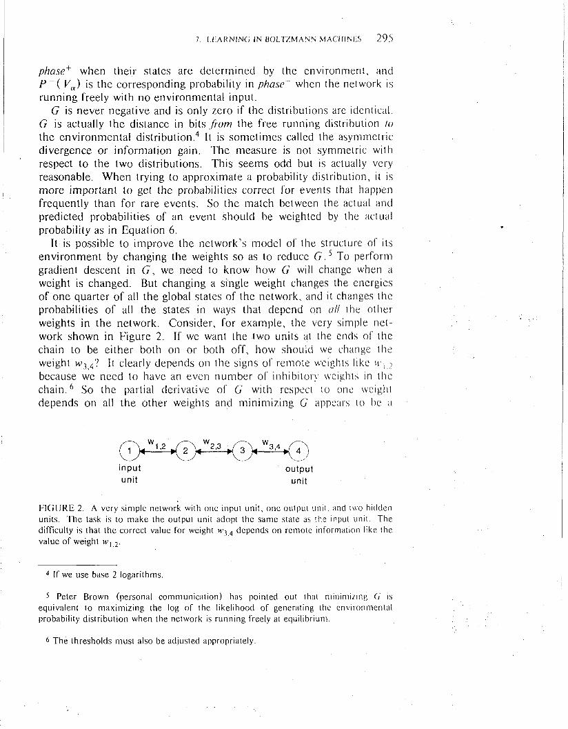
It is possible to improve the network's model of the structure of its environment by changing the weights s o as to reduce G ' To perform gradient descent in G , we need to know how G wrll change when a weight is changed. But changing a single weight changes the energles of o n e quarter of all the global states of the network, and i t change5 the probabilities of all the states In ways that depend on 011 the other weights in t he network. Consider, for example, the very s ~ m p l e net- work shown in Figure 2. If we want the two units at the end5 of the chain to be either both on or both off, how should we change thc weight w 3 4? I t clearly depends on the slgns of remote ue1gh15 l ~ k e because we need to have an even number of i nh~b~ to r ! \reightb In rhc chain. So the partial der iva t~ve of G w ~ t h re5pecL to onc wo~ght depends on all the other weights and minimizing G nppears I O be 'i

input unit

output unit

FIGURE 2 A very s ~ r n p l e network w ~ t h o n e Input unlt, o n e output unlt dnd Iiro h ~ d d e n unlts T h e task is t o m a k e the output unlt adopt t h e s a m e state 'is the Input unlt T h e d~ff icul ty IS that t h e correct value for weight w 3 depends o n remote ~nfornintion Itke the value of w e ~ g h t w

4 If we use base 2 logarithms.

5 Peter Brown (personal communicat ion) has pointed out that minimizing G is equivalent t o maximizing t h e log of t h e likelihood of generating the environmental probability distribution when the network is running freely at equilibrium.

6 T h e thresholds mus t also be adjusted appropriately

difficult computational problem that requires nonlocal information. Fortunately, all the information that is required about the other

weights in order to change w,, appropriately shows up in the behavior of the i t h and j t h units at thermal equilibrium. In addition to perform- ing a search for low energy states of the network, the process of reach- ing thermal equilibrium ensures that the joint activity of any two units contains all the information required for changing the weight between them in order to give the network a better model of its environment. T h e joint activity implicitly encodes information about all the other weights in the network. T h e Appendix shows that

where p,: is the probability, averaged over all environmental inputs and measured at equilibrium, that the i t h and j t h units are both on when the network is being driven by the environment, and p,; is the corresponding probability when the network is free running. One surprising feature of Equation 7 is that i t does not matter whether the weight is between two visible units, two hidden units, or one of each. T h e same rule applies for the gradient of G .

Unlearning

Crick and Mitchison (1983) have suggested that a form of reverse learning might occur during REM sleep in mammals. Their proposal was based on the assumption that parasitic modes develop in large net- works that hinder the distributed storage and retrieval of information. T h e mechanism that Crick and Mitchison propose is based on

More o r less random stimulation of the forebrain by the brain s tem that will tend to stimulate the inappropriate modes of brain activity . . . and especially those which are too prone to be set off by random noise rather than by highly structured specific signals. (p. 1 12)

During this state of random excitation and free running they postulate that changes occur at synapses to decrease the probability of the spurious states.

A simulation of reverse learning was performed by Hopfield, Fein- stein, and Palmer (1983) who independently had been studying ways to improve the associative storage capacity of simple networks of binary processors (Hopfield, 1982). In their algorithm an input is presented to the network as an initial condition, and the system evolves by falling

into a nearby local energy minimum. However, not all local energy minima represent stored information. In creating the desired minima, they accidentally create other spurious minima, and ro eliminate these they use "unlearning": T h e learning procedure is applied with reverse sign to the states found after starting from random initial conditions. Following this procedure, the performance of the system in accessing stored states was found to be improved.

There is an interesting relationship between the reverse learning pro- posed by Crick and Mitchison and Hopfield et al. and the form of rhe learning algorithm which we derived by considering how to minimize an information theory measure of the discrepancy between the environ- mental structure and the network's internal model (1-Iinton & Sejnowski, 1983b). T h e two phases of our learning algorithm resemble the learning and unlearning procedures: Positive Hebbian learning occurs in phase.+ during which information in the environ~iient is cap- tured by the weights; during phase- the system randomly samples states according to their Boltzmann distribution and Hebbian learning occurs with a negative coefficient.

However, these two phases need not be implemented in the manner suggested by Crick and Mitchison. For example. during pI1a.s.c the average co-occurrences could be computed without rnaking any changes to the weights. These averages could then be used as a baseline for making changes during phasef; that is, the co-occurrences during p/ ia~o ' could be computed and the baseline subtracred before each per- manent weight change. Thus , an alternative but equivalenr proposal for- the function of dream sleep is to recalibrate the baseline for- plasticity-the break-even point which determines whether a synaptic weight is incremented or decremented. This would be safer than mak- ing permanent weight decrements to synaptic weights during sleep and solves the problem of deciding how much "unlearning" to do.

Our learning algorithm refines Crick and Mitchison's interpretation of why two phases a re needed. Consider a hidden unit deep within the network: How should its connections with other units be changed to best capture regularity present in the environment? If i t 'does not receive direct input f rom the environment, the hidden unit has no way to determine whether t he information it receives from neighboring units is ultimately caused by structure in the environment or is entirely a result of the other weights. This can lead to a "folie a deux" where two parts of t he network each construct a model of the other and ignore the external environment. T h e contribution of internal and external sources can be separated by comparing the co-occurrences in phasef with similar information that is collected in the absence of environmental input. phase- thus acts as a control condition. Because of the special properties of equilibrium it is possible to subtract off this

purely internal contribution and use the difference to update the weights. 'Thus, the role of the two phases is to make the system maxi- -- mally responsive to regularities present in the environment and to prevent the system from using its capacity to model internally- generated regularities.

Ways in Which t h e Learning Algor i thm C a n Fail

The ability to discover the partial derivative of 6 by observing /I,;

and p; does not completely determine the learning algorithm. I t is still necessary to decide how much to change each weight, how long to col- lect co-occurrence statistics before changing the weight, how many weights to change at a time, and what temperature schedule to use dur- ing the annealing searches. For very simple networks in very simple environments, i t is possible to discover reasonable values for these parameters by trial and error. For more complex and interesting cases, serious difficulties arise because it is very easy to violate the assump- tions on which the mathematical results are based (Derthick, 1984).

The first difficulty is that there is nothing to prevent the learning algorithm from generating very large weights which create such high energy barriers that the network cannot reach equilibrium in the allot- ted time. Once this happens, the statistics that are collected will not be the equilibrium statistics required for Equation 7 to hold and so all bets are off. We have observed this happening for a number of different networks. They start off learning quite well and then the weights become too large and the network "goes souru-its performance deteriorates dramatically.

One way to ensure that the network gets close to equilibrium is to keep the weights small. Pearlmutter (personal communication) has shown that the learning works much better if, in addition to the weight changes caused by the learning, every weight continually decays towards a value of zero, with the speed of the decay being proportional to the absolute magnitude of the weight. This keeps the weights small and eventually leads to a relatively stable situation in which the decay rate of a weight is balanced by the partial derivative of G with respect to the weight. This has the satisfactory property that the absolute magnitude of a weight shows how important it is for modeling the environmental structure.

T h e use of weight-decay has several other consequences which are not s o desirable. Because the weights stay small, the network cannot construct very deep minima in the energy landscape and so it cannot make the probability ratios for similar global states be very different.

This means that i t is bound to give a significant number of errors in modeling environments where very similar vectors have very different probabilities. Better pe~forrnance can be achieved by annealing the net- work t o a lower final temperature (which is equivalent to making all the weights larger), but this will make the learning worse for two separate reasons. First, with less errors there is less to drive the learning because it relies o n the difference between the phase' and phase- statistics. Second, i t will be harder to reach thermal equilibrium at this lower temperature and so the co-occurrence statistics will be unreliable. O n e way of getting good statistics to drive the learning and also getting very few overt errors is to measure the co-occurrence statistics at a temperature higher than the final one.

Another way of ensuring that the network approaches equilibrium is to eliminate deep, narrow minima that are often not found by the annealing process. Derthick (1984) has shown that this can be done using a longer gentler annealing schedule in phase-. This means that the network is more likely to occupy the hard-to-find minima in phase- than in phase', and s o these minima will get filled in because the learn- ing rule raises the energies of states that are occupied more in phase- than in phase+.

A N EXAMPLE OF HARD LEARNING

A simple example which can only be solved by capturing the higher order statistical structure in the ensemble of input vectors is the "shifter" problem. T h e visible units are divided into three groups. Group V 1 is a one-dimensional array of 8 units, each of which is clamped o n or off at random with a probability of 0.3 of being on . Group V, also contains 8 units and their states are determined by shift- ing and copying the states of the units in group V,. T h e only shifts allowed are o n e to the left, one to the right, or no shift. Wrap-around is used s o that when there is a right shift, the state of the right-most unit in V , determines the state of the left-most unit in V2. The three possible shifts a re chosen at random with equal probabilities. Group V 3 contains three units to represent the three possible shifts, so at any o n e t ime o n e of t hem is clamped on and the others are clamped off.

T h e problem is t o learn the structure that relates the states of the three groups. O n e facet of this problem is to "recognize" the shift- i.e., to complete a partial input vector in which the states of V, and V2 are clamped but t he units in V3 are left free. It is fairly easy to see why this problem cannot possibly be solved by just adding together a lot of pairwise interactions between units in V,, V,, and V3 . If you know

that a particular unit in V1 is on , it tells you nothing whatsoever about what t hesh i f t is. It is only by finding combinations of active units in V1 and V2 that it is possible to predict the shift, so the information required is of at least third-order. This means that extra hidden units are required to perform the task.

T h e obvious way to recognize the shift is to have extra units which detect informative features such as an active unit in Vl and an active unit o n e place to the right in V2 and then support the unit V3 that represents a right shift. T h e empirical question is whether the learning algorithm is capable of turning some hidden units into feature detectors of this kind, and whether it will generate a set of detectors that work well together rather than duplicating the same detector. T h e set of weights that minimizes G defines t he optimal set of detectors but i t is not at all obvious what these detectors are, nor is i t obvious that the learning algorithm is capable of finding a good set.

Figure 3 shows the result of running a version of the Boltzniann machine learning procedure. Of the 24 hidden units, 5 seem to be doing very little but the remainder a re sensible looking detectors and most of them have become spatially localized. One type of detector which occurs several times consists of two large negative weights, one above the other, flanked by smaller excitatory weights on each side. This is a more discriminating detector of no-shift than simply having two positive weights, one above the other. It interesting to note that the various instances of this feature type all have different locations in V, and V2, even though the hidden units are not connected to each other. T h e pressure for the feature detectors to be different from each other comes from the gradient of G , rather than from the kind of lateral inhibition among the feature detectors that is used in "competi- tive learning" paradigms (Fukushima, 1980; Rumelhart & Zipser, 1985).

The Training Procedure

T h e training procedure alternated between two phases. In phase', all the units in V,, V2, and V3 were clamped into states representing a pair of 8-bit vectors and their relative shift. T h e hidden units were then allowed to change their states until the system approached thermal equilibrium at a temperature of 10. T h e annealing schedule is described below. After annealing, t he network was assumed to be close to thermal equilibrium and it was then run for a further 10 iterations during which t ime the frequency with which each pair of connected units were both o n was measured. This was repeated 20 times with

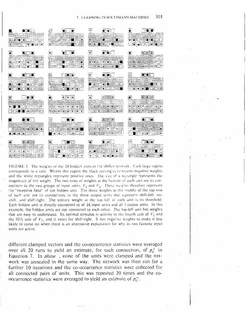
F I G U R E 3. 'The w e i g h ~ ~ ol'thc 24 hidden units In the jh~l'tcr ni . l \ r .c~r l \ 1:ach large region corresponds to a unit. Within this region the black rectangle, ri.prc\ent ncgatiw weight\ iind the white rectangles represent positive ones. The .;i/e 01' ;I sc~,tangle represents the magnitude of the weight. The two rows of weights at the t>ottonl of' e;~cli unit are its con- nections to the two groups 01' input units, I", and C'2. T-he\c wc~ght\ t h e r c l ' o ~ ~ ~ represe~it the "receptive lield" of the hidden unit. The three we~ghls In the middle 01' the top row 01' each unit are its connections to the three output units that ~reprcsent shift-left. n o - shil't, k~nd shift-right. The solitary weight at the top Icl't 01' ~ ~ c h u n i ~ ij its threshold. Each hidden unit is directly connected to all 16 input units and all 3 output units. In this example, the hidden units are not connected to each other. The top-left unit has weights that are easy to understand: Its optimal stimulus is activity in tho I'ourth unit of I / , and the fifih unit of V 2 , and i t votes for shift-right. I t has negative u ~ l g h t s to rnake i t less likely to come on when there is an alternative explanation for wh! its two favorite input units are active.

different clamped vectors and the co-occurrence stat~stics were averaged over all 20 runs to yield an estimate, for each connection, of p,f in Equation 7. In phase-, none of the units were clamped and the net- work was annealed in the same way. T h e network was then run for a further 10 iterations and the co-occurrence statistics were collected for all connected pairs of units. This was repeated 20 times and the co- occurrence statistics were averaged to yield an estimate of p,;.

302 BASIC MECfIANlSMS

T h e entire set of 40 annealings that were used to estimate p,; and p,; was called a sweep. After each sweep, every weight was incremented by 5(p,: - p,;). In addition, every weight had its absolute magnitude decreased by 0.0005 times its absolute magnitude. This weight decay prevented the weights from becoming too large and it also helped to resuscitate hidden units which had predominantly negative or predom- inantly positive weights. Such units spend all their t ime in the same state and therefore convey no information. T h e phase' and phase- statistics are identical for these units, and so the weight decay gradually erodes their weights until they come back to life (units with all zero weights come on half the t ime).

The Annealing Schedule

T h e annealing schedule spent the following number of iterations at the following temperatures: 2 at 40, 2 at 35, 2 at 30, 2 at 25, 2 at 20, 2 at 15, 2 at 12, 2 at 10. One iteration is defined as the number of ran- dom probes required so that each unit is probed one time on average. When it is probed, a unit uses its energy gap to decide which of its two states to adopt using the stochastic decision rule in Equation 3. Since each unit gets to see the most recent states of all the other units. an iteration cannot be regarded as a single parallel step. An truly parallel asynchronous system must tolerate t ime delays. Units must decide on their new states without being aware of very recent changes in the states of other units. It can be shown (Sejnowski, Hinton, Kienker, & Schumacher, 1985) that first-order time delays act like added tempera- ture and can therefore be tolerated by networks of this kind.

The Performance of the Shifter Network

T h e shifter network is encouraging because it is a clear example of the kind of learning of higher order structure that was beyond the capa- bility of perceptrons, but it also illustrates several weaknesses in the current approach.

T h e learning was very slow. 1t required 9000 learning sweeps, each of which involved reaching equilibrium 20 times in phasef with vectors clamped o n V1, V Z , and V3, and 20 times in phase- with n o units clamped. Even for low-level perceptual learning, this seems excessively slow.

T h e weights are fairly clearly not optimal because of the 5 hid- den units that app'ear to d o nothing useful. Also, the performance is far from perfect. When the states of the units in V , and V2 are clamped and the network is annealed gently to half the final temperature used during learning, the units in V 3 quite frequently adopt the wrong states. If the number of on units in V , is 1,2,3,4,5,6,7, the percentage of correctly recog- nized shifts is 50°/o, 719'0, 81°h, 86%, 89%, 82%, anti 66% respectively. The wide variation in the number of active units in V , naturally makes the task harder to learn than if a constant proportion of the units were active. Also, some of the input patterns are ambiguous. When all the units in V , and V 2 are off, the network can do no better than chance.

ACHIEVING RELIABLE COMPUTATION WITH UNRELIABLE HARDWARE

Conventional computers only work if all their individual components work perfectly, so as systems become larger they become more and more unreliable. Current computer technology uses extremely reliable components and error-correcting memories to achieve overall reliability. T h e brain appears to have much less reliable components, and so i t must use much more error-correction. I t is conceivable that the brain uses the kinds of representations that would be appropriate given reli- able hardware and then superimposes redundancy to compensate for its unreliable hardware.

T h e reliability issue is typically treated as a tedious residual problem to be dealt with after the main decisions about the form of the compu- tation have been made. A more direct approach is to treat reliability as a serious design constraint from the outset and to choose a basic style of computation that does not require reliable components. Ideally, we want a system in which none of the individual components are critical to the ability of the whole system to meet its requirements. In other words, we want s o m e high-level description of the behavior of the sys- tem to remain valid even when the low-level descriptions of the behavior of s o m e of the individual components change. This is only possible if the high-level description is related to the low level descrip- tions in a particular way: Every robust high-level property must be implemented by the combined effect of many local components, and n o single component must be crucial for the realization of the high-level property. This makes distributed representations (see Chapter 3) a natural choice when designing a damage-resistant system.

Distributed representations tend to behave robustly because they have an internal coherence which leads to an automatic "clean-up" effect. This effect can be seen in the patterns of activity that occur within a group of units and also in the interactions between groups. If a group of units, A, has a number of distinct and well-defined energy minima then these minima will remain even if a few units are removed or a little noise is added to many of the connections within A. T h e damage may distort the minima slightly and i t may also change their relative probabilities, but minor damage will not alter the gross topogra- phy of the energy landscape, so it will not affect higher level descrip- tions that depend only on this gross topography.

Even if the patterns of activity in A are slightly changed, this will often have no effect on the patterns caused in other groups of units. If the weights between groups of units have been fixed so that a particular pattern in A regularly causes a particular pattern in B, a small variation in the input coming from A will typically make no difference to the pat- tern that gets selected in B, because this pattern has its own internal coherence, and if the input from A is sufficiently accurate to select approximately the right pattern, the interactions among the elements in B will ensure that the details are right.

Damage resistance can be achieved by using a simple kind of representation in which there are many identical copies of each type of unit and each macroscopic item is encoded by activity in all the units of one type, In the undamaged system all these copies behave identically and a lot of capacity is therefore wasted. If we use distributed representations in which each unit may be used for representing many different i tems we can achieve comparable resistance to damage without wasting capacity. Because all the units behave differently from each other , t he undamaged system can implement many fine distinctions in the fine detail of the energy landscape. At the macroscopic level, these fine distinctions will appear as somewhat unreliable probabilistic ten- dencies and will be very sensitive to minor damage.

T h e fine details in the current energy landscape may contain the seeds of future changes in the gross topography. If learning novel dis- tinctions involves the progressive strengthening of regularities that a re initially tentative and unreliable, then it follows that learning may well suffer considerably when physical damage washes out these minor regularities. However, the simulations described below d o not bear on this interesting issue.

AN EXAMPLE OF THE EFFECTS OF DAMAGE

T o show the effects of damage o n a network, it is necessary to choose a task for the network to perform. Since we are mainly

concerned with properties that are fairly domain-independent, the details of the task are n@ especially relevant here. For reasons described in Chapter 3, we were interested in networks that can learn a n arbitrary mapping between items in two different domains, and we use that network to investigate the effects of damage. As we shall see, t he fact that the task involves purely arbitrary associations makes i t easier to interpret some of the interesting transfer effects that occur when a network relearns after sustaining major damage.

The Network

T h e network consisted of three groups or layers of units. T h e gra- pheme group was used to represent the letters in a three-letter word. It contained 30 units and was subdivided into three groups of 10 units each. Each subgroup was dedicated to o n e of the three letter positions within a word, and it represented one of the 10 possible letters in that position by having a single active unit for that letter. T h e three-letter grapheme strings were not English words. They were chosen randomly, subject to t he constraint that each of the 10 possible graphemes in each position had to be used at least once. T h e sen~eme group was used to encode the semantic features of the "word."' I t contained 30 units, one for each possible semantic feature The semantic features to be associ- ated with a word were chosen randomly, with each feature having a probability of 0.2 of being chosen for each word. There were connec- t ions between all pairs of units in the sememe group to allow the net- work to learn familiar combinations of semantic features. There were n o direct connections between the grapheme and sememe groups. Instead, there was an intermediate layer of 20 units, each of which was connected to all the units in both the grapheme and the semenie groups. Figure 4 is an artist's impression of the network. It uses English letters and words to convey the functions of the units in t he various layers. Most of the connections are missing.

The Training Procedure

T h e network was trained to associate each of 20 patterns of activity in t he grapheme units with an arbitrarily related pattern in the sememe

7 The representation of meaning 1s clearly more complicated than just a set of features, so the use of the word "semantic" here should not be taken too literally.

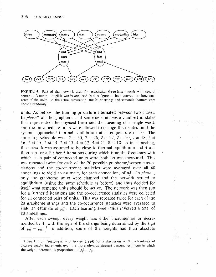
FIGURE 4. Part of the network used for associating three-letter words with sets of semantic features. English words are used in this figure to help convey the functional roles of the units. In the actual simulation, the letter-strings and semantic features were chosen randomly.

units. As before, the training procedure alternated between two phases. In phase+ all the grapheme and sememe units were clamped in states that represented the physical form and the meaning of a single word, and the intermediate units were allowed to change their states until the system approached thermal equilibrium at a temperature of 10. The annealing schedule was: 2 at 30, 2 at 26, 2 at 22, 2 at 20, 2 at 18, 2 at 16, 2 at 15, 2 at 14, 2 at 13, 4 at 12, 4 at 11, 8 at 10. After annealing, the network was assumed to be close to thermal equilibrium and it was then run for a further 5 iterations during which t ime the frequency with which each pair of connected units were both o n was measured. This was repeated twice for each of the 20 possible graphemelsememe asso- ciations and the co-occurrence statistics were averaged over all 40 annealings to yield an estimate, for each connection, of p;. In phase-, only the grapheme units were clamped and the network settled to equilibrium (using the same schedule as before) and thus decided for itself what s ememe units should be active. T h e network was then run for a further 5 iterations and the co-occurrence statistics were collected for all connected pairs of units. This was repeated twice for each of the 20 grapheme strings and the co-occurrence statistics were averaged to yield an estimate of p i . Each learning sweep thus involved a total of 80 annealings.

After each sweep, every weight was either incremented or decre- mented by 1, with the sign of the change being determined by the sign of p: - p . In addition, some of the weights had their absolute

8 See Hinton, Sejnowski, and Ackley (1984) for a discussion of the advantages of discrete weight increments over the more obvious steepest descent technique in which the weight increment is proportional to p g - pi,-.

magnitude decreased by 1. For each weight, the probability of this hap- pening was 0.0005 times the absolute magnitude of the weight.

We found that the network performed better if there was a preliminary learning stage which just involved the sememe units. In this stage, the intermediate units were not yet connected. During phasef the required patterns were clamped on the senieme units and p,: was measured (annealing was not required because all the units involved were clamped). During phase- no units were clamped and the network was allowed to reach equilibrium 20 times using the annealing schedule given above. After annealing, p,; was estimated from the co- occurrences as before, except that only 20 phase- annealings were used instead of 40. There were 300 sweeps of this learning stage and they resulted in weights between pairs of sememe units that were sufficient to give the sememe group an energy landscape with 20 strong minima corresponding to the 20 possible "word meanings." This helped subse- quent learning considerably, because it reduced the tendency for the intermediate units to be recruited for the job of modeling the structure among the sememe units. They were therefore free to model the struc- ture between the grapheme units and the sememe units.9 The results described here were obtained using the preliminary learning stage and so they correspond to learning to associate grapheme strings with "meanings" that are already familiar.

The Performance of the Network

Using the same annealing schedule as was used during learning, the network can be tested by clamping a grapheme string and looking at the resulting activities of the sememe units. After 5000 learning sweeps, it gets the semantic features exactly correct 99.3% of the time. A performance level of 99.9% can be achieved by using a "careful" annealing schedule that spends twice as long at each temperature and goes down to half the final temperature.

The Effect of Local Damage

T h e learning procedure generates weights which cause each of the units in the intermediate layer to be used for many different words.

9 There was no need to have a similar stage for learning the structure among the gra- pheme units because in the main stage of learning the grapheme units are always clamped and so there is no tendency for the network to try to model the structure among them.

This kind of distributed representation should be more tolerant of local damage than the more obvious method of using one intermediate unit per word. W e were particularly interested in the pattern of errors pro- duced by local damage. If the connections between sememe units are left intact, they should be able to "clean up" patterns of activity that are close to familiar ones. So the network should still produce perfect out- put even if the input to the sememe units is slightly disrupted. I f the disruption is more severe, the clean-up effect may actually produce a d@erent familiar meaning that happens to share the few semantic features that were correctly activated by the intermediate layer.

T o test these predictions we removed each of the intermediate units in turn, leaving the other 19 intact. We tested the network 25 times on each of the 20 words with each of the 20 units removed. In all 10,000 tests, using the careful annealing schedule, i t made 140 errors (98.6% correct). Many errors consisted of the correct set of semantic features with one or two extra or missing features, but 83 of the errors consisted of the precise meaning of some other grapheme string. An analysis of these 83 errors showed that the hamming distance between the correct meanings and the erroneous ones had a mean of 9.34 and a standard deviation of 1.27 which is significantly lower ( p < .01) than the com- plete set of hamming distances which had a mean of 10.30 and a stan- dard deviation of 2.41. We also looked at the hamming distances between the grapheme strings that the network was given as input and the grapheme strings that corresponded to the erroneous familiar mean- ings. T h e mean was 3.95 and the standard deviation was 0.62 which is significantly lower ( p < .01) than the complete set which had mean 5.53 and standard deviation 0.87. (A hamming distance of 4 means that the strings have one letter in common.)

In summary, when a single unit is removed from the intermediate layer, the network still performs well. The majority of its errors consist of producing exactly the meaning of some other grapheme string, and the erroneous meanings tend to be similar to the correct one and to be associated with a grapheme string that has one letter in common with the string used as input.

The Speed of Relearning

T h e original learning was very slow. Each item had to be presented 5000 times to eliminate almost all the errors. One reason for the slow- ness is the shape of the G-surface in weight-space. It tends to have long diagonal ravines which can be characterized in the following way: In the direction of steepest descent, the surface slopes steeply down for

7. L E A R N I N G IN BOLTZMANN MAC'I1INES 309

a short distance and then steeply up again (like the cross-section of a ravine).I0 l n most other directions the surface slopes gently upwards. In a relatively narrow cone of directions, the surface slopes gently down with very low curvature. This narrow cone corresponds to the floor of the ravine and to get a low value of G (which is the definition of good performance) the learning must follow the floor of the ravine without going u p the sides. This is particularly hard in a high-dimensional space. Unless t he gradient of the surface is measured very accurately, a s tep in t he direction of the estimated gradient will have a component along the floor of the ravine and a component up one of the many sides of t he ravine. Because the sides a re much steeper than the floor, t he result of the step will be to raise the value of G which makes performance worse. Once out of the bottom of the ravine, almost all the measurable gradient will be down towards the floor of the ravine instead of along the ravine. As a result, the path followed in weight space tends to consist of an irregular sloshing across the ravine with only a small amount of forward progress. W e are investigating ways of ameliorating this difficulty, but i t is a well-known problem of gradient descent techniques in high-dimensional spaces, and i t niay be unavoidable.

T h e ravine problem leads to a very interesting prediction about relearning when random noise is added to the weights. T h e original learning takes the weights a considerable distance along a ravine which is slow and difficult because most directions in weight space are up the sides of t he ravine. When a lot of random noise is added, there will typically be a small component along the ravine and a large component up the sides. Performance will therefore get much worse (because height in this space means poor performance), but relearning will be fast because the network can get back most of its performance by sim- ply descending to the floor of the ravine (which is easy) without niak- ing progress along the ravine (which is hard).

T h e s a m e phenomenon can be understood by considering the energy . landscape rather than the weight-space (recall that o n e point in weight- space constitutes a whole energy landscape). Good performance requires a rather precise balance between the relative depths of the 20 energy minima and it also requires that all the 20 minima have consid- erably lower energy than other parts of the energy landscape. T h e bal- ance between the minima in energy-space is the cross-section of t he ravine in weight-space (see Figure 5 ) and the depth of all t he minima compared with the rest of the energy landscape corresponds to the direction along the ravine. Random noise upsets the precise balance

l o The surface is never very steep. Its gradient parallel to any weight axis must always lie between 1 and - 1 because i t is the difference of two probabilities.

3 10 BASIC MECHANISMS

increase weights that help B -b

FIGURE 5 . One cross-section of a ravine in weight-space. Each point in weight space corresponds to a whole energy landscape. T o indicale (his, we show how a very simple landscape changes as the weights a re changed. Movement to the right along the x-axis corresponds to increasing the weights between pairs of units that are both on in state B and not both o n in state A. This increases the depth of A. If the task requires that A and B have about the same depth, an imbalance between them will lower the performance and thus raise G.

between the various minima without significantly affecting the gross topography of the energy landscape. Relearning can then restore most of the performance by restoring the balance between the existing minima.

The simulation behaved as predicted. The mean absolute value of the weights connecting the intermediate units to the other two groups was 21.5. These weights were first perturbed by adding uniform ran- dom noise in the range -2 to +2. This had surprisingly little effect, reducing the performance using the normal annealing schedule from 99.3% to 98.0%. This shows that the network is robust against slight noise in the weights. To cause significant deterioration, uniform ran- dom noise between -22 and +22 was added. On average, this perturbs each weight by about half its magnitude which was enough to reduce normal performance to 64.3% correct. Figure 6 shows the course of the relearning and compares it with the speed of the original learning when performance was at this level. It also shows that other kinds of damage produce very similar relearning curves.

I

0 5 10 15 20 25 30

Learning sweeps

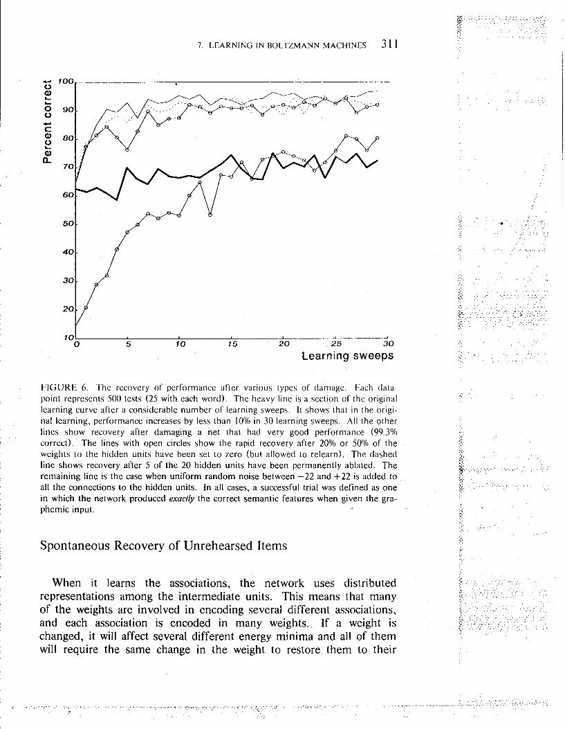
FIGURE 6. The recovery of performance after various types of damage. Each data- point represents 500 tests (25 with each word). The heavy line is a section of the original learning curve after a considerable number of learning sweeps. I t shows that in the origi- nal learning, performance increases by less than 10°/o in 30 learning sweeps. All the other lines show recovery after damaging a net that had very good performance (99.3% correct). The lines with open circles show the rapid recovery after 20% or 50% of the weights to the hidden units have been set to zero (but allowed to relearn). The dashed line shows recovery after 5 of the 20 hidden units have been permanently ablated. The remaining line is the case when uniform random noise between -22 and f 2 2 is added to all the connections to the hidden units. In all cases, a successful trial was defined as one in which the network produced exactly the correct semantic features when given the gra- phemic input.

Spontaneous Recovery of Unrehearsed Items

When it learns the associations, the network uses distributed representations among the intermediate units. This means that many of the weights are involved in encoding several different associations, and each association is encoded in many weights. If a weight is changed, it will affect several different energy minima and all of them will require the same change in the weight to restore them to their

3 12 BASIC MECHANISMS

previous depths. So, in relearning any one of the associations, there should be a positive transfer effect which tends to restore the others. This effect is actually rather weak and is easily masked so i t can only be seen clearly if we retrain the network on most of the original associa- tions and watch what happens to the remaining few. As predicted, these showed a marked improvement even though they were only ran- domly related to the associations on which the network was retrained.

W e took exactly the same perturbed network as before (uniform ran- dom noise between +22 and -22 added to the connections to and from the intermediate units) and retrained it on 18 of the associations for 30 learning sweeps. T h e two associations that were not retrained were selected to be ones where the network made frequent minor errors even when the careful annealing schedule was used. As a result of the retraining, the performance on these two items rose from 301100 correct to 90/100 correct with the careful schedule, but the few errors that remained tended to be completely wrong answers rather than minor perturbations of the correct answer. We repeated the experiment selecting two associations for which the error rate was high and the errors were typically large. Retraining on the other 18 associations caused a n improvement from 17/100 correct to 981100 correct. Despite these impressive improvements, the effect disappeared when we retrained o n only 15 of the associations. The remaining 5 actually got slightly worse. I t is clear that the fraction of the associations which needs to be retrained to cause improvement in the remainder depends o n how distributed the representations are, but more analys~s is required to characterize this relationship properly.

T h e spontaneous recovery of unrehearsed items seems paradoxical because the set of 20 associations was randomly generated and so there is n o way of generalizing from the 18 associations on which the net- work is retrained to the remaining two. During the original learning, however, t he weights capture regularities in the whole set of associa- tions. In this example, t he regularities are spurious but the network doesn't know that-it just finds whatever regularities i t can and expresses the associations in terms of them. Now, consider two dif- ferent regularities that a re equally strong among 18 of the associations. If o n e regularity also holds for the remaining two associations and the other doesn't, t he first regularity is more likely to be captured by the weights. During retraining, the learning procedure restores the weights to the values needed t o express the -regularities it originally chose to capture and it therefore tends to restore the remaining associations.

It would be interesting to see if any of the neuro-psychological data on the effects of brain damage could be interpreted in terms of the kinds of qualitative effects exhibited by the simulation when it is

damaged and relearns. However, we have not made any serious attempt t o fit the simulatiofl to particular data.

CONCLUSION

W e have presented three ideas:

Networks of symmetrically connected, binary units can escape from local minima during a relaxation search by using a sto- . . chastic decision rule.

T h e process of reaching thermal equilibrium in a network of stochastic units propagates exactly the information needed to d o credit assignment. This makes possible a local learning rule which can modify the weights so as to create new and useful feature detectors. The learning rule only needs to observe how often two units are both active (at thermal equilibrium) in two different phases. It can then change the weight between the units to make the spontaneous behavior of the network in one phase mimic the behavior that is forced on i t in the other phase.

T h e learning rule tends to construct distributed representations which are resistant to minor damage and exhibit rapid relearn- ing after major damage. The relearning process can bring back associations that are not practiced during the relearning and are only randomly related to the associations that are practiced.

These three ideas can be assessed separately. In particular, resistance to damage, rapid relearning, and spontaneous recovery of unrehearsed items can be exhibited by other kinds of parallel network that use distributed representations. The use of stochastic units, annealing search, and the two-phase learning algorithm are not crucial for these properties, though they are a convenient testbed in which to investigate them. Hogg and Huberman (1984) have demonstrated self-repair effects in nonstochastic, layered networks similar to those used by Fukushima (1980).

W e have left many loose ends, some of which are discussed else- where. Sejnowski and Hinton (in press) give a detailed example of a search problem where annealing helps, and they also discuss the rela- tionship between between these networks and the mammalian cortex. Ackley, Hinton, and Sejnowski (1985) give a different example of

learning in which the network constructs efficient internal codes for communicating information across narrow bandwidth channels. At present, the learning algorithm is too slow to be tested properly on large networks and future progress hinges on being able to speed i t up.

ACKNOWLEDGMENTS

This research was supported by grants from the System Development Foundation. W e thank David Ackley, Peter Brown, Francis Crick, Mark Derthick, Scott Fahlman, Stuart Geman, John Hopfield, Paul Kienker, Jay McClelland, Barak Pearlmutter, David Rumelhart, Tim Shallice, and Paul Smolensky for helpful discussions.

7 L E A R N I N G IN BOLTZMANN MACIiINES 315

APPENDIX: DERIVATION OF THE, LEARNING ALGORITHM

When a network is free-running at equilibrium the probability distrib- ution over the visible units is given by

xp- Emil 1 ( 8 )

P - ( v ) = C P - ( V,,A H@) = P

LY

@ x $ / A l*

where V,, is a vector of the states of the visible units, Ha is a vector of states of the hidden units, and E,, is the energy of the system in state V,Y Hp

E,,, = - x w, s , "hs ; '@. [ < I

Hence,

Differentiating ( 8 ) then yields

This derivative is used to compute the gradient of the G-measure

where p + ( V a ) is the clamped probability distribution over the visible units and is independent of w U . So

Now,

P + ( V , A H,,) = p + ( H p I

P-(v ,AH, , ) = p-(HpI

and

Equation 9 holds because the probability of a hidden state given some visible state must be the same in equilibrium whether the visible units were clamped in that state or arrived there by free-running. Hence,

Also,

Therefore,

where

and

The Boltzmann machine learning algorithm can also be formulated as an input-output model. The visible units are divided into an input set I and an output set 0, and an environment specifies a set of conditional probabilities of the form P + (Og I I,). During phasef the environment

7. LEARNING I N BOLTZMANN MACI-IINES 3 17

clamps both the input and output units, and the p,Ts are estimated. During phase- the inputsunits are clamped and the output units and hidden units free-run, and the p,;s are estimated. The appropriate G measure in this case is

P+(O, I I,) G = ~ P + ( I , A O,)ln

cx P P - ( O p 1 IJ -

Similar mathematics apply in this formulation and aG/a wi, is the same as before.