explorations in parallel distributed processing: a ... · explorations in parallel distributed...
TRANSCRIPT

Explorations in Parallel DistributedProcessing: A Handbook of Models,
Programs, and Exercises
Vesion 3.0
November 8, 2014
James L. McClelland
Printer-Friendly PDF Version
Send comments and corrections to:[email protected]
Send software issues and bug reports to:[email protected]

2

Contents
Preface v
1 Introduction 11.1 WELCOME TO THE NEW PDP HANDBOOK . . . . . . . . . 11.2 MODELS, PROGRAMS, CHAPTERS AND EXERCISES . . . . 2
1.2.1 Key Features of PDP Models . . . . . . . . . . . . . . . . 21.3 SOME GENERAL CONVENTIONS AND CONSIDERATIONS 4
1.3.1 Mathematical Notation . . . . . . . . . . . . . . . . . . . 41.3.2 Pseudo-MATLAB Code . . . . . . . . . . . . . . . . . . . 51.3.3 Program Design and User Interface . . . . . . . . . . . . . 51.3.4 Exploiting the MATLAB Environment . . . . . . . . . . . 6
1.4 BEFORE YOU START . . . . . . . . . . . . . . . . . . . . . . . 61.5 MATLAB MINI-TUTORIAL . . . . . . . . . . . . . . . . . . . . 7
1.5.1 Basic Operations . . . . . . . . . . . . . . . . . . . . . . . 71.5.2 Vector Operations . . . . . . . . . . . . . . . . . . . . . . 81.5.3 Logical operations . . . . . . . . . . . . . . . . . . . . . . 101.5.4 Control Flow . . . . . . . . . . . . . . . . . . . . . . . . . 111.5.5 Vectorized Code . . . . . . . . . . . . . . . . . . . . . . . 12
2 Interactive Activation and Competition 152.1 BACKGROUND . . . . . . . . . . . . . . . . . . . . . . . . . . . 15
2.1.1 How Competition Works . . . . . . . . . . . . . . . . . . . 192.1.2 Resonance . . . . . . . . . . . . . . . . . . . . . . . . . . . 192.1.3 Hysteresis and Blocking . . . . . . . . . . . . . . . . . . . 202.1.4 Grossberg’s Analysis of Interactive Activation and Com-
petition Processes . . . . . . . . . . . . . . . . . . . . . . 202.2 THE IAC MODEL . . . . . . . . . . . . . . . . . . . . . . . . . . 21
2.2.1 Architecture . . . . . . . . . . . . . . . . . . . . . . . . . 222.2.2 Visible and Hidden Units . . . . . . . . . . . . . . . . . . 222.2.3 Activation Dynamics . . . . . . . . . . . . . . . . . . . . . 222.2.4 Parameters . . . . . . . . . . . . . . . . . . . . . . . . . . 222.2.5 Pools and Projections . . . . . . . . . . . . . . . . . . . . 232.2.6 The Core Routines . . . . . . . . . . . . . . . . . . . . . . 24
2.3 EXERCISES . . . . . . . . . . . . . . . . . . . . . . . . . . . . . 28
i

ii CONTENTS
3 Constraint Satisfaction in PDP Systems 413.1 BACKGROUND . . . . . . . . . . . . . . . . . . . . . . . . . . . 413.2 THE SCHEMA MODEL . . . . . . . . . . . . . . . . . . . . . . . 453.3 IMPLEMENTATION . . . . . . . . . . . . . . . . . . . . . . . . 463.4 RUNNING THE PROGRAM . . . . . . . . . . . . . . . . . . . . 48
3.4.1 Reset, Newstart, and the Random Seed . . . . . . . . . . 483.4.2 Options and parameters . . . . . . . . . . . . . . . . . . . 48
3.5 OVERVIEW OF EXERCISES . . . . . . . . . . . . . . . . . . . 493.6 GOODNESS AND PROBABILITY . . . . . . . . . . . . . . . . 55
3.6.1 Local Maxima . . . . . . . . . . . . . . . . . . . . . . . . 563.6.2 Escaping from Local Maxima . . . . . . . . . . . . . . . . 66
4 Learning in PDP Models: The Pattern Associator 674.1 BACKGROUND . . . . . . . . . . . . . . . . . . . . . . . . . . . 68
4.1.1 The Hebb Rule . . . . . . . . . . . . . . . . . . . . . . . . 684.1.2 The Delta Rule . . . . . . . . . . . . . . . . . . . . . . . . 704.1.3 Division of Labor in Error Correcting Learning . . . . . . 734.1.4 The Linear Predictability Constraint . . . . . . . . . . . . 74
4.2 THE PATTERN ASSOCIATOR . . . . . . . . . . . . . . . . . . 744.2.1 The Hebb Rule in Pattern Associator Models . . . . . . . 764.2.2 The Delta Rule in Pattern Associator Models . . . . . . . 794.2.3 Linear Predictability and the Linear Independence Re-
quirement . . . . . . . . . . . . . . . . . . . . . . . . . . . 814.2.4 Nonlinear Pattern Associators . . . . . . . . . . . . . . . . 82
4.3 THE FAMILY OF PATTERN ASSOCIATOR MODELS . . . . . 824.3.1 Activation Functions . . . . . . . . . . . . . . . . . . . . . 834.3.2 Learning Assumptions . . . . . . . . . . . . . . . . . . . . 834.3.3 The Environment and the Training Epoch . . . . . . . . . 844.3.4 Performance Measures . . . . . . . . . . . . . . . . . . . . 84
4.4 IMPLEMENTATION . . . . . . . . . . . . . . . . . . . . . . . . 854.5 RUNNING THE PROGRAM . . . . . . . . . . . . . . . . . . . . 88
4.5.1 Commands and Parameters . . . . . . . . . . . . . . . . . 894.5.2 State Variables . . . . . . . . . . . . . . . . . . . . . . . . 90
4.6 OVERVIEW OF EXERCISES . . . . . . . . . . . . . . . . . . . 914.6.1 Further Suggestions for Exercises . . . . . . . . . . . . . . 103
5 Training Hidden Units with Backpropagation 1055.1 BACKGROUND . . . . . . . . . . . . . . . . . . . . . . . . . . . 105
5.1.1 Minimizing Mean Squared Error . . . . . . . . . . . . . . 1095.1.2 The Backpropagation Rule . . . . . . . . . . . . . . . . . 113
5.2 IMPLEMENTATION . . . . . . . . . . . . . . . . . . . . . . . . 1245.3 RUNNING THE PROGRAM . . . . . . . . . . . . . . . . . . . . 1275.4 EXERCISES . . . . . . . . . . . . . . . . . . . . . . . . . . . . . 128

CONTENTS iii
6 Competitive Learning 1396.1 SIMPLE COMPETITIVE LEARNING . . . . . . . . . . . . . . 139
6.1.1 Background . . . . . . . . . . . . . . . . . . . . . . . . . . 1396.1.2 Some Features of Competitive Learning . . . . . . . . . . 1466.1.3 Implementation . . . . . . . . . . . . . . . . . . . . . . . . 1476.1.4 Overview of Exercises . . . . . . . . . . . . . . . . . . . . 148
6.2 SELF-ORGANIZING MAP . . . . . . . . . . . . . . . . . . . . . 1506.2.1 The Model . . . . . . . . . . . . . . . . . . . . . . . . . . 1516.2.2 Some Features of the SOM . . . . . . . . . . . . . . . . . 1526.2.3 Implementation . . . . . . . . . . . . . . . . . . . . . . . . 1546.2.4 Overview of Exercises . . . . . . . . . . . . . . . . . . . . 157
7 The Simple Recurrent Network: A Simple Model that Capturesthe Structure in Sequences 1657.1 BACKGROUND . . . . . . . . . . . . . . . . . . . . . . . . . . . 165
7.1.1 The Simple Recurrent Network . . . . . . . . . . . . . . . 1657.1.2 Graded State Machines . . . . . . . . . . . . . . . . . . . 173
7.2 THE SRN PROGRAM . . . . . . . . . . . . . . . . . . . . . . . 1757.2.1 Sequences . . . . . . . . . . . . . . . . . . . . . . . . . . . 1757.2.2 New Parameters . . . . . . . . . . . . . . . . . . . . . . . 1767.2.3 Network specification . . . . . . . . . . . . . . . . . . . . 1777.2.4 Fast mode for training . . . . . . . . . . . . . . . . . . . 177
7.3 EXERCISES . . . . . . . . . . . . . . . . . . . . . . . . . . . . . 177
8 Recurrent Backpropagation: Attractor network models of se-mantic and lexical processing 1838.1 BACKGROUND . . . . . . . . . . . . . . . . . . . . . . . . . . . 1838.2 THE RBP PROGRAM . . . . . . . . . . . . . . . . . . . . . . . 185
8.2.1 Time intervals, and the partitioning of intervals into ticks 1868.2.2 Visualizing the state space of an rbp network . . . . . . . 1868.2.3 Forward propagation of activation. . . . . . . . . . . . . . 1888.2.4 Backward propagation of error . . . . . . . . . . . . . . . 1898.2.5 Calculating the weight error derivatives . . . . . . . . . . 1908.2.6 Updating the weights. . . . . . . . . . . . . . . . . . . . . 190
8.3 Using the rbp program with the rogers network . . . . . . . . . . 1928.3.1 rbp fast training mode. . . . . . . . . . . . . . . . . . . . 1928.3.2 Training and Lesioning with the rogers network . . . . . . 1938.3.3 rbp pattern files. . . . . . . . . . . . . . . . . . . . . . . . 1948.3.4 Creating an rbp network . . . . . . . . . . . . . . . . . . 194
9 Temporal-Difference Learning 1979.1 BACKGROUND . . . . . . . . . . . . . . . . . . . . . . . . . . . 1979.2 REINFORCEMENT LEARNING . . . . . . . . . . . . . . . . . 202
9.2.1 Discounted Returns . . . . . . . . . . . . . . . . . . . . . 2039.2.2 The Control Problem . . . . . . . . . . . . . . . . . . . . 204
9.3 TD AND BACKPROPAGATION . . . . . . . . . . . . . . . . . 207

iv CONTENTS
9.3.1 Back Propagating TD Error . . . . . . . . . . . . . . . . . 2089.3.2 Case Study: TD-Gammon . . . . . . . . . . . . . . . . . . 210
9.4 IMPLEMENTATION . . . . . . . . . . . . . . . . . . . . . . . . 2129.4.1 Specifying the Environment . . . . . . . . . . . . . . . . . 214
9.5 RUNNING THE PROGRAM . . . . . . . . . . . . . . . . . . . . 2189.6 EXERCISES . . . . . . . . . . . . . . . . . . . . . . . . . . . . . 220
A PDPTool Version 3 Installation and Quick Start Guide 223A.1 Introduction and System requirements . . . . . . . . . . . . . . . 223A.2 Installation . . . . . . . . . . . . . . . . . . . . . . . . . . . . . . 223A.3 Using PDPTool at a Stanford Cluster Computer . . . . . . . . . 224A.4 Using the software . . . . . . . . . . . . . . . . . . . . . . . . . . 224
B How to Create your own Network 225B.1 Creating the Network Initialization Script . . . . . . . . . . . . . 226
B.1.1 Initializing and Quitting the Software With or Withoutthe Gui . . . . . . . . . . . . . . . . . . . . . . . . . . . . 226
B.1.2 Defining the Network Pools . . . . . . . . . . . . . . . . . 227B.1.3 Defining the Connections Between Pools . . . . . . . . . . 227B.1.4 Creating the Network Object . . . . . . . . . . . . . . . . 228B.1.5 Associating an Environment and a Display template with
the Network . . . . . . . . . . . . . . . . . . . . . . . . . . 228B.2 Format for Pattern Files . . . . . . . . . . . . . . . . . . . . . . . 229B.3 Creating the Display Template . . . . . . . . . . . . . . . . . . . 229B.4 Setting Parameters in the Initialization Script and Loading Saved
Weights . . . . . . . . . . . . . . . . . . . . . . . . . . . . . . . . 234B.5 Logging and Graphing Network Variables . . . . . . . . . . . . . 236B.6 Additional Commands; Using the Initialization Script as a Batch
Process Script . . . . . . . . . . . . . . . . . . . . . . . . . . . . . 239B.7 The PDPlog file . . . . . . . . . . . . . . . . . . . . . . . . . . . . 239
C PDPTool User’s Guide 241
D PDPTool Standalone Executable 243D.1 Installing under Linux . . . . . . . . . . . . . . . . . . . . . . . . 243D.2 Running under Linux . . . . . . . . . . . . . . . . . . . . . . . . . 246D.3 Installing under Windows . . . . . . . . . . . . . . . . . . . . . . 246D.4 Running under Windows . . . . . . . . . . . . . . . . . . . . . . . 247D.5 Installing under Mac OSX . . . . . . . . . . . . . . . . . . . . . . 249D.6 Running under Mac OSX . . . . . . . . . . . . . . . . . . . . . . 251

Preface
This work represents a continuing effort to make parallel-distributed process-ing models accessible and available to all who are interested in exploring them.The initial inspiration for the handbook and accompanying software came fromthe students who took the first version of what I called “the PDP class” whichI taught at Carnegie Mellon from about 1986 to 1995. Dave Rumelhart con-tributed extensively to the first edition (McClelland and Rumelhart, 1988), andof course the book incorporated many of the insights and exercises that Davidcontributed to the original PDP Books (Rumelhart et al., 1986; McClellandet al., 1986).
In the mid-1990’s, I moved on to other teaching commitments and turnedteaching of the course over to David Plaut. Dave used the PDP handbook andsoftware initially, but, due to some limitations in coverage, shifted over to usingthe LENS simulation environment (Rohde, 1999). Rohde’s simulator is very fastand is highly recommended for full strengh, large-training-set, neural networksimulations. My lab is now maintaining a version of LENS, available by clicking‘Source Code’ at this link.
Upon my move to Stanford in the fall of 2006 I found myself teaching thePDP class again, and at that point I decided to update the original handbook.The key decisions were to keep the core ideas of the basic models as they wereoriginally described; re-implement everything in MATLAB; update the book byadding models that had become core parts of the framework as I know it in theinterim; and make both the handbook and the software available on line.
This version of the handbook documents PDPTool 3.0, a new version of thesoftware available for use as of August, 2014. Information on installation ofthe software is provided in Appendix A. Appendix B presents a step-by-stepexample showing how a user can create a simple backpropagation network, andAppendix C offers a User’s Guide, approximating an actual reference manualfor the software itself. The hope is that, once the framework is in place, wecan make it easy for others to add new models and exercises to the framework.If you have one you’d like us to incorporate, please let me know and I’ll beglad to work with you on setting it up. Reports of software bugs or installationdifficulties should be sent to [email protected].
Before we start, I’d like to acknowledge the people who have made the newversion of the PDP software a reality. Most important are Sindy John, a pro-grammer who has been working with me for nearly 5 years, and Brenden Lake,
v

vi PREFACE
a former Stanford Symbolic Systems major. Sindy had done the vast major-ity of the coding in the current version of the pdptool software, and wrote theUser’s Guide. Brenden helped convert several chapters, and added the mate-rial on Kohonen networks in Chapter 6. He has also helped tremendously withthe implementation of the on-line version of the handbook. Two other Sym-bolic Systems undergraduates also contributed quite a bit: David Ho wrote theMATLAB tutorial in Chapter 1, and Anna Schapiro did the initial conversionof Chapter 3.
It is tragic that David Rumelhart is no longer able to contribute, leaving mein the position as sole author of this work. I have been blessed and honored,however, to work with many wonderful collaborators, post-docs, and studentsover the years, and to have benefited from the insights of many others. Allthese people are the authors of the ideas presented here, and their names willbe found in references cited throughout this handbook.
Jay McClellandStanford, CASeptember, 2011

Chapter 1
Introduction
1.1 WELCOME TO THE NEW PDP HAND-BOOK
Several years ago, Dave Rumelhart and I first developed a handbook to introduceothers to the parallel distributed processing (PDP) framework for modelinghuman cognition. When it was first introduced, this framework represented anew way of thinking about perception, memory, learning, and thought, as wellas a new way of characterizing the computational mechanisms for intelligentinformation processing in general. Since it was first introduced, the frameworkhas continued to evolve, and it is still under active development and use inmodeling many aspects of cognition and behavior.
Our own understanding of parallel distributed processing came about largelythrough hands-on experimentation with these models. And, in teaching PDP toothers, we discovered that their understanding was enhanced through the samekind of hands-on simulation experience. The original edition of the handbookwas intended to help a wider audience gain this kind of experience. It mademany of the simulation models discussed in the two PDP volumes (Rumelhartet al., 1986; McClelland et al., 1986) available in a form that is intended tobe easy to use. The handbook also provided what we hoped were accessibleexpositions of some of the main mathematical ideas that underlie the simulationmodels. And it provided a number of prepared exercises to help the reader beginexploring the simulation programs.
The current version of the handbook attempts to bring the older handbookup to date. Most of the original material has been kept, and a good deal ofnew material has been added. All of simulation programs have been imple-mented or re-implemented within the MATLAB programming environment. Inkeeping with other MATLAB projects, we call the suite of programs we haveimplemented the PDPTool software.
Although the handbook presents substantial background on the computa-tional and mathematical ideas underlying the PDP framework, it should be used
1

2 CHAPTER 1. INTRODUCTION
in conjunction with additional readings from the PDP books and other sources.In particular, those unfamiliar with the PDP framework should read Chapter 1of the first PDP volume (Rumelhart et al., 1986) to understand the motivationand the nature of the approach.
This chapter provides some general information about the software and thehandbook. The chapter also describes some general conventions and designdecisions we have made to help the reader make the best possible use of thehandbook and the software that comes with it. Information on how to setup the software (Appendix A), and a user’s guide (Appendix C), are providedin Appendices. At the end of the chapter we provide a brief tutorial on theMATLAB computing environment, within which the software is implemented.
1.2 MODELS, PROGRAMS, CHAPTERS ANDEXERCISES
The PDPTool software consists of a set of programs, all of which have a similarstructure. Each program implements several variants of a single PDP modelor network type. The programs all make use of the same interface and displayroutines, and most of the commands are the same from one program to thenext.
Each program is introduced in a new chapter, which also contains relevantconceptual background for the type of PDP model that is encompassed by theprogram, and a series of exercises that allow the user to explore the propertiesof the models considered in the chapter.
In view of the similarity between the simulation programs, the informationthat is given when each new program is introduced is restricted primarily towhat is new. Readers who wish to dive into the middle of the book, then, mayfind that they need to refer back to commands or features that were introducedearlier. The User’s Guide provides another means of learning about specificfeatures of the programs.
1.2.1 Key Features of PDP Models
Here we briefly describe some of the key features most PDP models share. Fora more detailed presentation, see Chapter 2 of the PDP book (Rumelhart et al.,1986).
A PDP model is built around a simulated artificial neural network, whichconsists of units organized into pools, and connections among these units or-ganized into projections. The minimal case (shown in Figure 2.1) would be anetwork with a single pool of units and a single projection from each unit in thenetwork to every other unit. The basic idea is that units propagate excitatoryand inhibitory signals to each other via the weighted connections. Adjustmentsmay occur to the strengths of the connections as a result of processing. The unitsand connections constitute the architecture of the network, within which theseprocesses occur. Units in a network may receive external inputs (usually from

1.2. MODELS, PROGRAMS, CHAPTERS AND EXERCISES 3
Figure 1.1: A simple PDP network consisting of one pool of units, and oneprojection, such that each unit receives connections from all other units in thesame pool. Each unit also can receive external input (shown coming in from theleft). If this were a pool in a larger network, the units could receive additionalprojections from other pools (not shown) and could project to units in otherpools (as illustrated by the arrows proceeding out of the units to the right. (FromFigure 1, p. 162 in McClelland, J. L.& Rumelhart, D. E. (1985). Distributedmemory and the representation of general and specific information. Journalof Experimental Psychology: General, 114, 159-197. Copyright 1985 by theAmerican Psychological Association. Permission Pending.)
the network’s environment, described next), and outputs may be propagatedout of the network.
A PDP model also generally includes an environment, which consists ofpatterns that are used to provide inputs and/or target values to the network.An input pattern specifies external input values for a pool of units. A targetpattern specifies desired target activation values for units in a pool, for use intraining the network. Patterns can be grouped in various ways to structure theinput and target patterns presented to a network. Different groupings are usedin different programs.
A PDP model also consists of a set of processes, including a test processand possibly a train process, as well as ancillary processes for loading, saving,displaying, and re-initializing. The test process presents input patterns (or setsof input patterns) to the network, and causes the network to process the pat-terns, possibly comparing the results to provided target patterns, and possiblycomputing other statistics and/or saving results for later inspection. Process-ing generally takes place in a single step or through a sequence of processingcycles. Processing consists of propagating activation signals from units to otherunits, multiplying each signal by the connection weight on the connection tothe receiving unit from the sending unit. These weighted inputs are summed atthe receiving unit, and the summed value is then used to adjust the activations

4 CHAPTER 1. INTRODUCTION
of each receiving unit for the next processing step, according to a specified ac-tivation function. A train process presents a series of input patterns (or setsof input patterns), processes them using a process similar to the test process,then possibly compares the results generated to the values specified in targetpatterns (or sets of provided target patterns) and then carries out further pro-cessing steps that result in the adjustment of connections among the processingunits.
The exact nature of the processes that take place in both training and test-ing are essential ingredients of specific PDP models and will be considered as wework through the set of models described in this book. The models described inChapters 2 and 3 explore processing in networks with modeler-specified connec-tion weights, while the models described in most of the later chapters involvelearning as well as processing.
1.3 SOME GENERAL CONVENTIONS ANDCONSIDERATIONS
1.3.1 Mathematical Notation
We have adopted a mathematical notation that is internally consistent withinthis handbook and that facilitates translation between the description of themodels in the text and the conventions used to access variables in the programs.The notation is not always consistent with that introduced in the chapters ofthe PDP volumes or other papers. Here follows an enumeration of the keyfeatures of the notation system we have adopted. We begin with the conventionswe have used in writing equations to describe models and in explicating theirmathematical background.
Scalars. Scalar (single-valued) variables are given in italic typeface. The namesof parameters are chosen to be mnemonic words or abbreviations wherepossible. For example, the decay parameter is called decay.
Vectors. Vector (multivalued) variables are given in boldface; for example, theexternal input pattern is called extinput. An element of such a vectoris given in italic typeface with a subscript. Thus, the ith element of theexternal input is denoted extinputi. Vectors are often members of largersets of vectors; in this case, a whole vector may be given a subscript.For example, the jth input pattern in a set of patterns would be denotedipatternj.
Weight matrices. Matrix variables are given in uppercase boldface; for exam-ple, a weight matrix might be denoted W. An element of a weight matrixis given in lowercase italic, subscripted first by the row index and then bythe column index. The row index corresponds to the index of the receivingunit, and the column index corresponds to the index of the sending unit.

1.3. SOME GENERAL CONVENTIONS AND CONSIDERATIONS 5
Thus the weight to unit i from unit j would be found in the jth columnof the ith row of the matrix, and is written wij .
Counting. We follow the MATLAB language convention and count from 1.Thus if there are n elements in a vector, the indexes run from 1 to n. Timeis a bit special in this regard. Time 0 (t0) is the time before processingbegins; the state of a network at t0 can be called its “initial state.” Timecounters are incremented as soon as processing begins within each timestep.
1.3.2 Pseudo-MATLAB Code
In the chapters, we occasionally give pieces of computer code to illustrate theimplementation of some of the key routines in our simulation programs. Theexamples are written in “pseudo-MATLAB”; details such as declarations areleft out. Note that the pseudocode printed in the text for illustrating the imple-mentation of the programs is generally not identical to the actual source code;the program examples are intended to make the basic characteristics of the im-plementation clear rather than to clutter the reader’s mind with the details andspeed-up hacks that would be found in the actual programs.
Several features of MATLAB need to be understood to read the pseudo-MATLAB code and to work within the MATLAB environment. These arelisted in the MATLAB mini-tutorial given at the end of this chapter. Readersunfamiliar with MATLAB will want to consult this tutorial in order to be ableto work effectively with the PDPTool Software.
1.3.3 Program Design and User Interface
Our goals in writing the programs were to make them both as flexible as pos-sible and as easy as possible to use, especially for running the core exercisesdiscussed in each chapter of this handbook. We have achieved these somewhatcontradictory goals as follows. Flexibility is achieved by allowing the user tospecify the details of the network configuration and of the layout of the displaysshown on the screen at run time, via files that are read and interpreted by theprogram. Ease of use is achieved by providing the user with the files to run thecore exercises and by keeping the command interface and the names of variablesconsistent from program to program wherever possible. Full exploitation of theflexibility provided by the program requires the user to learn how to constructnetwork configuration files and display configuration (or template) files, but thisis only necessary when the user wishes to apply a program to some new problemof his or her own.
Another aspect of the flexibility of the programs is their permissiveness. Ingeneral, we have allowed the user to examine and set as many of the variables ineach program as possible, including basic network configuration variables thatshould not be changed in the middle of a run. The worst that can happen isthat the programs will crash under these circumstances; it is, therefore, wise

6 CHAPTER 1. INTRODUCTION
not to experiment with changing them if losing the state of a program would becostly.
1.3.4 Exploiting the MATLAB Environment
It should be noted that the implementation of the software within the MAT-LAB environment provides two sources of further flexibility. First, users witha full MATLAB license have access to the considerable tools of the MATLABenvironment available for their use in preparing inputs and in analyzing andvisualizing outputs from simulations. We have provided some hooks into thesevisualization tools, but advanced users are likely to want to exploit some of thefeatures of MATLAB for advanced analysis and visualization.
Second, because all of the source code is provided for all programs, it hasproven fairly straightforward for users with some programming experience todelve into the code to modify it or add extensions. Users are encouraged todive in and make changes. If you manage the changes you make carefully, youshould be able to re-implement them as patches to future updates.
1.4 BEFORE YOU START
Before you dive into your first PDP model, we would like to offer both anexhortation and a disclaimer. The exhortation is to take what we offer here,not as a set of fixed tasks to be undertaken, but as raw material for your ownexplorations. We have presented the material following a structured plan, butthis does not mean that you should follow it any more than you need to to meetyour own goals. We have learned the most by experimenting with and adaptingideas that have come to us from other people rather than from sticking closelyto what they have offered, and we hope that you will be able to do the samething. The flexibility that has been built into these programs is intended tomake exploration as easy as possible, and we provide source code so that userscan change the programs and adapt them to their own needs and problems asthey see fit.
The disclaimer is that we cannot be sure the programs are perfectly bugfree. They have all been extensively tested and they work for the core exercises;but it is possible that some users will discover problems or bugs in undertakingsome of the more open-ended extended exercises. If you have such a problem,we hope that you will be able to find ways of working around it as much aspossible or that you will be able to fix it yourself. In any case, please let us howof the problems you encounter (Send bug reports, problems, and suggestions toJay McClelland at [email protected]). While we cannot offer to provideconsultation or fixes for every reader who encounters a problem, we will useyour input to improve the package for future users.

1.5. MATLAB MINI-TUTORIAL 7
1.5 MATLAB MINI-TUTORIAL
Here we provide a brief introduction to some of the main features of the MAT-LAB computing environment. While this should allow readers to understandbasic MATLAB operations, there are a many features of MATLAB that are notcovered here. The built-in documentation in MATLAB is very thorough, andusers are encouraged to explore the many features of the MATLAB environmentafter reading this basic tutorial. There are also many additional MATLAB tu-torials and references available online; a simple Google search for ‘MATLABtutorial’ should bring up the most popular ones.
1.5.1 Basic Operations
Comments. Comments in MATLAB begin with “%”. The MATLAB inter-preter ignores anything to the right of the “%” character on a line. We use thisconvention to introduce comments into the pseudocode so that the code is easierfor you to follow.
% This is a comment.y = 2*x + 1 % So is this.
Variables. Addition (“+”), subtraction (“-”), multiplication (“*”), divi-sion (“/”), and exponentiation (“^”) on scalars all work as you would expect,following the order of operations. To assign a value to a variable, use “=”.
Length = 1 + 2*3 % Assigns 7 to the variable ’Length’.square = Length^2 % Assigns 49 to ’square’.triangle = square / 2 % Assigns 24.5 to ’triangle’.length = Length - 2 % ’length’ and ’Length’ are different.
Note that MATLAB performs actual floating-point division, not integer di-vision. Also note that MATLAB is case sensitive.
Displaying results of evaluating expressions. The MATLAB interpreterwill evaluate any expression we enter, and display the result. However, puttinga semicolon at the end of a line will suppress the output for that line. MATLABalso stores the result of the latest expression in a special variable called “ans”.
3*10 + 8 % This assigns 38 to ans, and prints ’ans = 38’.3*10 + 8; % This assigns 38 to ans, and prints nothing.
In general, MATLAB ignores whitespace; however, it is sensitive to linebreaks. Putting “...” at the end of a line will allow an expression on that lineto continue onto the next line.
sum = 1 + 2 - 3 + 4 - 5 + ... % We can use ’...’ to6 - 7 + 8 - 9 + 10 % break up long expressions.

8 CHAPTER 1. INTRODUCTION
1.5.2 Vector Operations
Building vectors Scalar values between “[” and “]” are concatenated intoa vector. To create a row vector, put spaces or commas between each of theelements. To create a column vector, put a semicolon between each of theelements.
foo = [1 2 3 square triangle] % row vectorbar = [14, 7, 3.62, 5, 23, 3*10+8] % row vectorxyzzy = [-3; 200; 0; 9.9] % column vector
To transpose a vector (turning a row vector into a column vector, or viceversa), use “’”.
foo’ % a column vector[1 1 2 3 5]’ % a column vectorxyzzy’ % a row vector
We can define a vector containing a range of values by using colon notation,specifying the first value, (optionally) an increment, and the last value.
v = 3:10 % This vector contains [3 4 5 6 7 8 9 10]w = 1:2:10 % This vector contains [1 3 5 7 9]x = 4:-1:2 % This vector contains [4 3 2]y = -6:1.5:0 % This vector contains [-6 -4.5 -3 -1.5 0]z = 5:1:1 % This vector is emptya = 1:10:2 % This vector contains [1]
We can get the length of a vector by using “length()”.
length(v) % 8length(x) % 3length(z) % 0
Accessing elements within a vector Once we have defined a vector andstored it in a variable, we can access individual elements within the vector bytheir indices. Indices in MATLAB start from 1. The special index ’end’ refersto the last element in a vector.
y(2) % -4.5w(end) % 9x(1) % 4
We can use colon notation in this context to select a range of values fromthe vector.
v(2:5) % [4 5 6 7]w(1:end) % [1 3 5 7 9]w(end:-1:1) % [9 7 5 3 1]y(1:2:5) % [-6 -4.5 0]

1.5. MATLAB MINI-TUTORIAL 9
In fact, we can specify any arbitrary “index vector” to select arbitrary ele-ments of the vector.
y([2 4 5]) % [-4.5 -1.5 0]v(x) % [6 5 4]w([5 5 5 5 5]) % [9 9 9 9 9]
Furthermore, we can change a vector by replacing the selected elements witha vector of the same size. We can even delete elements from a vector by assigningthe empty matrix “[]” to the selected elements.
y([2 4 5]) = [42 420 4200] % y = [-6 42 -3 420 4200]v(x) = [0 -1 -2] % v = [3 -2 -1 0 7 8 9 10]w([3 4]) = [] % w = [1 3 9]
Mathematical vector operations We can easily add (“+”), subtract (“-”),multiply (“*”), divide (“/”), or exponentiate (“.^”) each element in a vector bya scalar. The operation simply gets performed on each element of the vector,returning a vector of the same size.
a = [8 6 1 0]a/2 - 3 % [1 0 -2.5 -3]3*a.^2 + 5 % [197 113 8 5]
Similarly, we can perform “element-wise” mathematical operations betweentwo vectors of the same size. The operation is simply performed between ele-ments in corresponding positions in the two vectors, again returning a vector ofthe same size. We use “+” for adding two vectors, and “-” to subtract two vec-tors. To avoid conflicts with different types of vector multiplication and division,we use “.*” and “./” for element-wise multiplication and division, respectively.We use “.^” for element-wise exponentiation.
b = [4 3 2 9]a+b % [12 9 3 9]a-b % [4 3 -1 -9]a.*b % [32 18 2 0]a./b % [2 2 0.5 0]a.^b % [4096 216 1 0]
Finally, we can perform a dot product (or inner product) between a rowvector and a column vector of the same length by using (“*”). The dot productmultiplies the elements in corresponding positions in the two vectors, and thentakes the sum, returning a scalar value. To perform a dot product, the row vectormust be listed before the column vector (otherwise MATLAB will perform anouter product, returning a matrix).
r = [9 4 0]c = [8; 7; 5]r*c % 100

10 CHAPTER 1. INTRODUCTION
1.5.3 Logical operations
Relational operators We can compare two scalar values in MATLAB usingrelational operators: “==” (“equal to”), “~=” (“not equal to”), “<” (“less than”),“<=” (“less than or equal to”) “>” (“greater than”), and “>=” (“greater than orequal to”). The result is 1 if the comparison is true, and 0 if the comparison isfalse.
1 == 2 % 01 ~= 2 % 12 < 2 % 02 <= 3 % 1(2*2) > 3 % 13 >= (5+1) % 03/2 == 1.5 % 1
Note that floating-point comparisons work correctly in MATLAB.The unary operator “~” (“not”) flips a binary value from 1 to 0 or 0 to 1.
flag = (4 < 2) % flag = 0~flag % 1
Logical operations with vectors. As with mathematical operations, using arelational operator between a vector and a scalar will compare each each elementof the vector with the scalar, in this case returning a binary vector of the samesize. Each element of the binary vector is 1 if the comparison is true at thatposition, and 0 if the comparison is false at that position.
ages = [56 47 8 12 20 18 21]ages >= 21 % [1 1 0 0 0 0 1]
To test whether a binary vector contains any 1s, we use “any()”. To testwhether a binary vector contains all 1s, we use “all()”.
any(ages >= 21) % 1all(ages >= 21) % 0any(ages == 3) % 0all(ages < 100) % 1
We can use the binary vectors as a different kind of “index vector” to selectelements from a vector; this is called “logical indexing”, and it returns all of theelements in the vector where the corresponding element in the binary vector is1. This gives us a powerful way to select all elements from a vector that meetcertain criteria.
ages([1 0 1 0 1 0 1]) % [56 8 20 21]ages(ages >= 21) % [56 47 21]

1.5. MATLAB MINI-TUTORIAL 11
1.5.4 Control Flow
Normally, the MATLAB interpreter moves through a script linearly, executingeach statement in sequential order. However, we can use several structures tointroduce branching and looping into the flow of our programs.If statements. An if statement consists of: one if block, zero or more elseifblocks, and zero or one else block. It ends with the keyword end.
Any of the relational operators defined above can be used as a conditionfor an if statement. MATLAB executes the statements in an if block or aelseif block only if its associated condition is true. Otherwise, the MATLABinterpreter skips that block. If none of the conditions were true, MATLABexecutes the statements in the else block (if there is one).
team1_score = rand() % a random number between 0 and 1team2_score = rand() % a random number between 0 and 1
if(team1_score > team2_score)disp(’Team 1 wins!’) % Display "Team 1 wins!"
elseif(team1_score == team2_score)disp(’It’s a tie!’) % Display "It’s a tie!"
elsedisp(’Team 2 wins!’) % Display "Team 2 wins!"
end
In fact, instead of using a relational operator as a condition, we can useany expression. If the expression evaluates to anything other than 0, the emptymatrix [], or the boolean value false, then the expression is considered to be“true”.
While loops. A while loop works the same way as an if statement, exceptthat, when the MATLAB interpreter reaches the end keyword, it returns to thebeginning of the while block and tests the condition again. MATLAB executesthe statements in the while block repeatedly, as long as the condition is true. Abreak statement within the while loop will cause MATLAB to skip the rest ofthe loop.
i = 3while i > 0
disp(i)i = i - 1;
enddisp(’Blastoff!’)
% This will display:% 3% 2% 1% Blastoff!

12 CHAPTER 1. INTRODUCTION
For loops. To execute a block of code a specific number of times, we can use afor loop. A for loop takes a counter variable and a vector. MATLAB executesthe statements in the block once for each element in the vector, with the countervariable set to that element.
r = [9 4 0];c = [8 7 5];
sum = 0;for i = 1:3 % The counter is ’i’, and the range is ’1:3’
sum = sum + r(i) * c(i); % This will be executed 3 timesend
% After the loop, sum = 100
Although the “range” vector is most commonly a range of consecutive in-tegers, it doesn’t have to be. Actually, the range vector doesn’t even need tobe created with the colon operator. In fact, the range vector can be any vectorwhatsoever; it doesn’t even need to contain integers at all!
my_favorite_primes = [2 3 5 7 11]for order = [2 4 3 1 5]
disp(my_favorite_primes(order))end
% This will display:% 3% 7% 5% 2% 11
1.5.5 Vectorized Code
Vectorized code is code that describes (and, conceptually) executes mathemat-ical operations on vectors an matrices “all at once”. Vectorised code is truerto the parallel “spirit” of the operations being performed in linear algebra, andalso to the conceptual framework of PDP. Conceptually, the pseudocode descrip-tions of our algorithms (usually) should not involve the sequential repetition ofa for loop. For example, when computing the input to a unit from other units,there is no reason for the multiplication of one activation times one connectionweight to “wait” for the previous one to be completed. Instead, each multiplica-tion should be though of as being performed independently and simultaneously.And in fact, vectorized code can execute much faster that code written explicitlyas a for loop. This effect is especially pronounced when processing can be splitacross several processors.Writing vectorised code. Let’s say we have two vectors, r and c.

1.5. MATLAB MINI-TUTORIAL 13
r = [9 4 0];c = [8;7;5];
We have seen two ways to perform a dot product between these two vectors.We can use a for loop:
sum = 0;for i = 1:3
sum = sum + r(i) * c(i);end% After the loop, sum = 100
However, the following “vectorized” code is more concise, and it takes ad-vantage of MATLAB’s optimization for vector and matrix operations:
sum = r*c; % After this statement, sum = 100
Similarly, we can use a for loop to multiply each element of a vector by ascalar, or to multiply each element of a vector by the corresponding element inanother vector:
for i = 1:3r(i) = r(i) * 2;
end% After the loop, r = [18 8 0]
multiplier = [2;3;4];for j = 1:3
c(j) = c(j) * multiplier(j);end% After the loop, c = [16 21 20]
However, element-wise multiplication using .* is faster and more concise:
r * 2; % After this statement, r = [18 8 0]
multiplier = [2;3;4];c = c .* multiplier; % After this statement, c = [16 21 20]

14 CHAPTER 1. INTRODUCTION

Chapter 2
Interactive Activation andCompetition
Our own explorations of parallel distributed processing began with the use ofinteractive activation and competition mechanisms of the kind we will exam-ine in this chapter. We have used these kinds of mechanisms to model visualword recognition (McClelland and Rumelhart, 1981; Rumelhart and McClel-land, 1982) and to model the retrieval of general and specific information fromstored knowledge of individual exemplars (McClelland, 1981), as described inPDP:1. In this chapter, we describe some of the basic mathematical observa-tions behind these mechanisms, and then we introduce the reader to a specificmodel that implements the retrieval of general and specific information usingthe “Jets and Sharks” example discussed in PDP:1 (pp. 25-31).
After describing the specific model, we will introduce the program in whichthis model is implemented: the iac program (for interactive activation and com-petition). The description of how to use this program will be quite extensive; itis intended to serve as a general introduction to the entire package of programssince the user interface and most of the commands and auxiliary files are com-mon to all of the programs. After describing how to use the program, we willpresent several exercises, including an opportunity to work with the Jets andSharks example and an opportunity to explore an interesting variant of the basicmodel, based on dynamical assumptions used by Grossberg (e.g., (Grossberg,1978)).
2.1 BACKGROUND
The study of interactive activation and competition mechanisms has a longhistory. They have been extensively studied by Grossberg. A useful introductionto the mathematics of such systems is provided in Grossberg (1978). Relatedmechanisms have been studied by a number of other investigators, includingLevin (1976), whose work was instrumental in launching our exploration of
15

16 CHAPTER 2. INTERACTIVE ACTIVATION AND COMPETITION
PDP mechanisms.An interactive activation and competition network (hereafter, IAC network)
consists of a collection of processing units organized into some number of com-petitive pools. There are excitatory connections among units in different poolsand inhibitory connections among units within the same pool. The excitatoryconnections between pools are generally bidirectional, thereby making the pro-cessing interactive in the sense that processing in each pool both influences andis influenced by processing in other pools. Within a pool, the inhibitory con-nections are usually assumed to run from each unit in the pool to every otherunit in the pool. This implements a kind of competition among the units suchthat the unit or units in the pool that receive the strongest activation tend todrive down the activation of the other units.
The units in an IAC network take on continuous activation values betweena maximum and minimum value, though their output—the signal that theytransmit to other units—is not necessarily identical to their activation. In ourwork, we have tended to set the output of each unit to the activation of the unitminus the threshold as long as the difference is positive; when the activationfalls below threshold, the output is set to 0. Without loss of generality, we canset the threshold to 0; we will follow this practice throughout the rest of thischapter. A number of other output functions are possible; Grossberg (1978)describes a number of other possibilities and considers their various merits.
The activations of the units in an IAC network evolve gradually over time.In the mathematical idealization of this class of models, we think of the acti-vation process as completely continuous, though in the simulation modeling weapproximate this ideal by breaking time up into a sequence of discrete steps.Units in an IAC network change their activation based on a function that takesinto account both the current activation of the unit and the net input to theunit from other units or from outside the network. The net input to a particularunit (say, unit i) is the same in almost all the models described in this volume:it is simply the sum of the influences of all of the other units in the networkplus any external input from outside the network. The influence of some otherunit (say, unit j) is just the product of that unit’s output, outputj , times thestrength or weight of the connection to unit i from unit j. Thus the net inputto unit i is given by
neti =∑j
wijoutputj + extinputi. (2.1)
In the IAC model, outputj = [aj ]+. Here, aj refers to the activation of unit j,and the expression [aj ]+ has value aj for all aj > 0; otherwise its value is 0.The index j ranges over all of the units with connections to unit i. In generalthe weights can be positive or negative, for excitatory or inhibitory connections,respectively.
Human behavior is highly variable and IAC models as described thus far arecompletely deterministic. In some IAC models, such as the interactive activationmodel of letter perception (McClelland and Rumelhart, 1981) these determin-istic activation values are mapped to probabilities. However, it became clear in

2.1. BACKGROUND 17
detailed attempts to fit this model to data that intrinsic variability in processingand/or variability in the input to a network from trial to trial provided bettermechanisms for allowing the models to provide detailed fits to data. McClel-land (1991) found that injecting normally distributed random noise into the netinput to each unit on each time cycle allowed such networks to fit experimentaldata from experiments on the joint effects of context and stimulus informationon phoneme or letter perception. Including this in the equation above, we have:
neti =∑j
wijoutputj + extinputi + normal(0, noise) (2.2)
Where normal(0, noise) is a sample chosen from the standard normal dis-tribution with mean 0 and standard deviation of noise. For simplicity, noise isset to zero in many IAC network models.
Once the net input to a unit has been computed, the resulting change in theactivation of the unit is as follows:
If (neti > 0),
∆ai = (max− ai)neti − decay(ai − rest).
Otherwise,∆ai = (ai −min)neti − decay(ai − rest).
Note that in this equation, max, min, rest, and decay are all parameters. Ingeneral, we choose max = 1, min ≤ rest ≤ 0, and decay between 0 and 1. Notealso that ai is assumed to start, and to stay, within the interval [min,max].
Suppose we imagine the input to a unit remains fixed and examine what willhappen across time in the equation for ∆ai. For specificity, let’s just supposethe net input has some fixed, positive value. Then we can see that ∆ai will getsmaller and smaller as the activation of the unit gets greater and greater. Forsome values of the unit’s activation, ∆ai will actually be negative. In particular,suppose that the unit’s activation is equal to the resting level. Then ∆ai issimply (max − rest)neti. Now suppose that the unit’s activation is equal tomax, its maximum activation level. Then ∆ai is simply (−decay)(max− rest).Between these extremes there is an equilibrium value of ai at which ∆ai is 0.We can find what the equilibrium value is by setting ∆ai to 0 and solving forai:
0 = (max− ai)neti − decay(ai − rest)= (max)(neti) + (rest)(decay)− ai(neti + decay)
ai =(max)(neti) + (rest)(decay)
neti + decay(2.3)
Using max = 1 and rest = 0, this simplifies to
ai =neti
neti + decay(2.4)
What the equation indicates, then, is that the activation of the unit will reachequilibrium when its value becomes equal to the ratio of the net input divided by

18 CHAPTER 2. INTERACTIVE ACTIVATION AND COMPETITION
the net input plus the decay. Note that in a system where the activations of otherunits—and thus of the net input to any particular unit—are also continuallychanging, there is no guarantee that activations will ever completely stabilize—although in practice, as we shall see, they often seem to.
Equation 3 indicates that the equilibrium activation of a unit will alwaysincrease as the net input increases; however, it can never exceed 1 (or, in thegeneral case, max) as the net input grows very large. Thus, max is indeed theupper bound on the activation of the unit. For small values of the net input,the equation is approximately linear since x/(x + c) is approximately equal tox/c for x small enough.
We can see the decay term in Equation 3 as acting as a kind of restoringforce that tends to bring the activation of the unit back to 0 (or to rest, in thegeneral case). The larger the value of the decay term, the stronger this forceis, and therefore the lower the activation level will be at which the activationof the unit will reach equilibrium. Indeed, we can see the decay term as scalingthe net input if we rewrite the equation as
ai =neti/decay
(neti/decay) + 1(2.5)
When the net input is equal to the decay, the activation of the unit is 0.5 (in thegeneral case, the value is (max + rest)/2). Because of this, we generally scalethe net inputs to the units by a strength constant that is equal to the decay.Increasing the value of this strength parameter or decreasing the value of thedecay increases the equilibrium activation of the unit.
In the case where the net input is negative, we get entirely analogous results:
ai =(min)(neti)− (decay)(rest)
neti − decay(2.6)
Using rest = 0, this simplifies to
ai =(min)(neti)neti − decay
(2.7)
This equation is a bit confusing because neti and min are both negative quan-tities. It becomes somewhat clearer if we use amin (the absolute value of min)and aneti (the absolute value of neti). Then we have
ai = − (amin)(aneti)aneti + decay
(2.8)
What this last equation brings out is that the equilibrium activation value ob-tained for a negative net input is scaled by the magnitude of the minimum(amin). Inhibition both acts more quickly and drives activation to a lower finallevel when min is farther below 0.

2.1. BACKGROUND 19
2.1.1 How Competition Works
So far we have been considering situations in which the net input to a unit isfixed and activation evolves to a fixed or stable point. The interactive activa-tion and competition process, however, is more complicated than this becausethe net input to a unit changes as the unit and other units in the same poolsimultaneously respond to their net inputs. One effect of this is to amplifydifferences in the net inputs of units. Consider two units a and b that are mutu-ally inhibitory, and imagine that both are receiving some excitatory input fromoutside but that the excitatory input to a (ea) is stronger than the excitatoryinput to b (eb). Let γ represent the strength of the inhibition each unit exertson the other. Then the net input to a is
neta = ea − γ(outputb) (2.9)
and the net input to b is
netb = eb − γ(outputa) (2.10)
As long as the activations stay positive, outputi = ai, so we get
neta = ea − γab (2.11)
andnetb = eb − γaa (2.12)
From these equations we can easily see that b will tend to be at a disadvantagesince the stronger excitation to a will tend to give a a larger initial activation,thereby allowing it to inhibit b more than b inhibits a. The end result is aphenomenon that Grossberg (1976) has called “the rich get richer” effect: Unitswith slight initial advantages, in terms of their external inputs, amplify thisadvantage over their competitors.
2.1.2 Resonance
Another effect of the interactive activation process has been called “resonance”by Grossberg (1978). If unit a and unit b have mutually excitatory connections,then once one of the units becomes active, they will tend to keep each otheractive. Activations of units that enter into such mutually excitatory interactionsare therefore sustained by the network, or “resonate” within it, just as certainfrequencies resonate in a sound chamber. In a network model, depending onparameters, the resonance can sometimes be strong enough to overcome theeffects of decay. For example, suppose that two units, a and b, have bidirectional,excitatory connections with strengths of 2 x decay . Suppose that we set eachunit’s activation at 0.5 and then remove all external input and see what happens.The activations will stay at 0.5 indefinitely because
∆aa = (1− aa)neta − (decay)aa

20 CHAPTER 2. INTERACTIVE ACTIVATION AND COMPETITION
= (1− 0.5)(2)(decay)(0.5)− (decay)(0.5)
= (0.5)(2)(decay)(0.5)− (decay)(0.5)
= 0
Thus, IAC networks can use the mutually excitatory connections between unitsin different pools to sustain certain input patterns that would otherwise decayaway rapidly in the absence of continuing input. The interactive activationprocess can also activate units that were not activated directly by externalinput. We will explore these effects more fully in the exercises that are givenlater.
2.1.3 Hysteresis and Blocking
Before we finish this consideration of the mathematical background of interactiveactivation and competition systems, it is worth pointing out that the rate ofevolution towards the eventual equilibrium reached by an IAC network, andeven the state that is reached, is affected by initial conditions. Thus if at time0 we force a particular unit to be on, this can have the effect of slowing theactivation of other units. In extreme cases, forcing a unit to be on can totallyblock others from becoming activated at all. For example, suppose we have twounits, a and b, that are mutually inhibitory, with inhibition parameter gammaequal to 2 times the strength of the decay, and suppose we set the activationof one of these units—unit a—to 0.5. Then the net input to the other—unitb—at this point will be (-0.5) (2) (decay) = −decay. If we then supply externalexcitatory input to the two units with strength equal to the decay, this willmaintain the activation of unit a at 0.5 and will fail to excite b since its net inputwill be 0. The external input to b is thereby blocked from having its normaleffect. If external input is withdrawn from a, its activation will gradually decay(in the absence of any strong resonances involving a) so that b will graduallybecome activated. The first effect, in which the activation of b is completelyblocked, is an extreme form of a kind of network behavior known as hysteresis(which means “delay”); prior states of networks tend to put them into statesthat can delay or even block the effects of new inputs.
Because of hysteresis effects in networks, various investigators have sug-gested that new inputs may need to begin by generating a “clear signal,” oftenimplemented as a wave of inhibition. Such ideas have been proposed by variousinvestigators as an explanation of visual masking effects (see, e.g., (Weissteinet al., 1975)) and play a prominent role in Grossberg’s theory of learning inneural networks, see Grossberg (1980).
2.1.4 Grossberg’s Analysis of Interactive Activation andCompetition Processes
Throughout this section we have been referring to Grossberg’s studies of whatwe are calling interactive activation and competition mechanisms. In fact, he

2.2. THE IAC MODEL 21
uses a slightly different activation equation than the one we have presentedhere (taken from our earlier work with the interactive activation model of wordrecognition). In Grossberg’s formulation, the excitatory and inhibitory inputsto a unit are treated separately. The excitatory input (e) drives the activationof the unit up toward the maximum, whereas the inhibitory input (i) drives theactivation back down toward the minimum. As in our formulation, the decaytends to restore the activation of the unit to its resting level.
∆a = (max− a)e− (a−min)i− decay(a− rest) (2.13)
Grossberg’s formulation has the advantage of allowing a single equation togovern the evolution of processing instead of requiring an if statement to inter-vene to determine which of two equations holds. It also has the characteristicthat the direction the input tends to drive the activation of the unit is affectedby the current activation. In our formulation, net positive input will alwaysexcite the unit and net negative input will always inhibit it. In Grossberg’sformulation, the input is not lumped together in this way. As a result, theeffect of a given input (particular values of e and i) can be excitatory whenthe unit’s activation is low and inhibitory when the unit’s activation is high.Furthermore, at least when min has a relatively small absolute value comparedto max, a given amount of inhibition will tend to exert a weaker effect on a unitstarting at rest. To see this, we will simplify and set max = 1.0 and rest = 0.0.By assumption, the unit is at rest so the above equation reduces to
∆a = (1)e− (amin)(i) (2.14)
where amin is the absolute value of min as above. This is in balance only ifi = e/amin.
Our use of the net input rule was based primarily on the fact that we foundit easier to follow the course of simulation events when the balance of excitatoryand inhibitory influences was independent of the activation of the receivingunit. However, this by no means indicates that our formulation is superiorcomputationally. Therefore we have made Grossberg’s update rule availableas an option in the iac program. Note that in the Grossberg version, noise isadded into the excitatory input, when the noise standard deviation parameteris greater than 0.
2.2 THE IAC MODEL
The IAC model provides a discrete approximation to the continuous interactiveactivation and competition processes that we have been considering up to now.We will consider two variants of the model: one that follows the interactiveactivation dynamics from our earlier work and one that follows the formulationoffered by Grossberg.
The IAC model is part of the part of the PDPTool Suite of programs, whichrun under MATLAB. A document describing the overall structure of the PDP-

22 CHAPTER 2. INTERACTIVE ACTIVATION AND COMPETITION
tool called the PDPTool User Guide should be consulted to get a general un-derstanding of the structure of the PDPtool system.
Here we describe key characteristics of the IAC model software implemen-tation. Specifics on how to run exercises using the IAC model are provided asthe exercises are introduced below.
2.2.1 Architecture
The IAC model consists of several units, divided into pools. In each pool, allthe units are assumed to be mutually inhibitory. Between pools, units mayhave excitatory connections. In IAC models, the connections are generally bidi-rectionally symmetric, so that whenever there is an excitatory connection fromunit i to unit j, there is also an equal excitatory connection from unit j backto unit i. IAC networks can, however, be created in which connections violatethese characteristics of the model.
2.2.2 Visible and Hidden Units
In an IAC network, there are generally two classes of units: those that canreceive direct input from outside the network and those that cannot. The firstkind of units are called visible units; the latter are called hidden units. Thus inthe IAC model the user may specify a pattern of inputs to the visible units, butby assumption the user is not allowed to specify external input to the hiddenunits; their net input is based only on the outputs from other units to whichthey are connected.
2.2.3 Activation Dynamics
Time is not continuous in the IAC model (or any of our other simulation models),but is divided into a sequence of discrete steps, or cycles. Each cycle beginswith all units having an activation value that was determined at the end ofthe preceding cycle. First, the inputs to each unit are computed. Then theactivations of the units are updated. The two-phase procedure ensures thatthe updating of the activations of the units is effectively synchronous; that is,nothing is done with the new activation of any of the units until all have beenupdated.
The discrete time approximation can introduce instabilities if activationsteps on each cycle are large. This problem is eliminated, and the approxi-mation to the continuous case is generally closer, when activation steps are keptsmall on each cycle.
2.2.4 Parameters
In the IAC model there are several parameters under the user’s control andstored in a property of the network called test options. Most of these havealready been introduced. They are

2.2. THE IAC MODEL 23
max The maximum activation parameter.
min The minimum activation parameter.
rest The resting activation level to which activations tend to settle in the ab-sence of external input.
decay The decay rate parameter, which determines the strength of the ten-dency to return to resting level.
estr This parameter stands for the strength of external input (i.e., input tounits from outside the network). It scales the influence of external signalsrelative to internally generated inputs to units.
alpha This parameter scales the strength of the excitatory input to units fromother units in the network.
gamma This parameter scales the strength of the inhibitory input to unitsfrom other units in the network.
In general, it would be possible to specify separate values for each of theseparameters for each unit. The IAC model does not allow this, as we have foundit tends to introduce far too many degrees of freedom into the modeling process.However, the model does allow the user to specify strengths for the individualconnection strengths in the network.
The noise parameter is treated separately in the IAC model. Here, thereis a pool-specific variable called ’noise’. How this actually works is describedunder Core Routines below.
2.2.5 Pools and Projections
The main thing to understand about the way networks work is to understandthe concepts pool and projection. A pool is a set of units and a projection is aset of connections linking two pools. A network could have a single pool anda single projection, but usually networks have more constrained architecturesthan this, so that a pool and projection structure is appropriate.
All networks have a special pool called the bias pool that contains a singleunit called the bias unit that is always on. The connection weights from thebias pool to the units in another pool can take any value, and that value thenbecomes a constant part of the input to the unit. The bias pool is alwayspools(1). A network with a layer of input units and a layer of hidden unitswould have two additional pools, pools(2) and pools(3) respectively.
Projections connect the units from one pool to those connected to it fromanother pool. The first projection to each pool is the projection from the biaspool, if such a projection is used (there is no such projection in the jets net-work). A projection can connect a pool to itself or connect one pool to anotherpool. In the jets network, there is a pool for the visible units and a pool for thehidden units, and there is a self-projection (projection 1 in each case) containing

24 CHAPTER 2. INTERACTIVE ACTIVATION AND COMPETITION
mutually inhibitory connections and also a projection from the other pool (pro-jection 2 in each case) containing between-pool excitatory connections. Theseconnections are bi-directionally symmetric.
The connection to visible unit i from hidden unit j is:
net.pools(2).projections(2).using.weights(i, j)
and the symmetric return connection is
net.pools(3).projections(2).using.weights(j, i)
2.2.6 The Core Routines
Here we explain the basic structure of the core routines used in the iac program.Note that the use of obj in each function refers locally to the net object beingmanipulated by the function. That is, the net object is passed as the argumentto the functions where it is then referred to locally as obj.
reset net. This routine is used to reset the activations of units to their restinglevels and to reset the time—the current cycle number—back to 0. Allvariables are cleared, and the display is updated to show the networkbefore processing begins.
cycle. This routine is the basic routine that is used in running the model. Itcarries out a number of processing cycles, as determined by the programcontrol variable ncycles. On each cycle, two routines are called: getnetand update. At the end of each cycle, if pdptool is being run in gui mode,then the program checks to see whether the display is to be updated andwhether to pause so the user can examine the new state (and possiblyterminate processing) with a function called done updating cycleno. Theroutine looks like this:
function cycle(obj)obj.getnet;obj.update;end
The test routine looks like this:
function test(obj)
while obj.next_cycleno <= obj.test_options.ncyclesobj.cycleno = obj.next_cycleno;obj.cycle;obj.next_cycleno = obj.cycleno + 1;
\%what follows is concerned with pausing\%and updating the display

2.2. THE IAC MODEL 25
if obj.done_updating_cyclenoreturn
endend
The getnet and update routines are somewhat different for the standardversion and Grossberg version of the program. We first describe the stan-dard versions of each, then turn to the Grossberg versions. In both routines,the version to be used is determined by a switch statement on the value ofnet.test options.actfunction, which can be ’st’ for standard or ’gr’ for Gross-berg.
Standard getnet. The standard getnet routine computes the net input foreach pool. The net input consists of three things: the external input, scaled byestr; the excitatory input from other units, scaled by alpha; and the inhibitoryinput from other units, scaled by gamma. For each pool, the getnet routine firstaccumulates the excitatory and inhibitory inputs from other units, then scalesthe inputs and adds them to the scaled external input to obtain the net input. Ifthe pool-specific noise parameter is non-zero, a sample from the standard normaldistribution is taken, then multiplied by the value of the ’noise’ parameter, thenadded to the excitatory input.
Whether a connection is excitatory or inhibitory is determined by its sign.The connection weights from every sending unit to a pool(w) are examined. Forall positive values of w, the corresponding excitation terms are incremented bypools(sender).activation(index)∗w(w > 0). This operation uses MATLAB log-ical indexing to apply the computation to only those elements of the array thatsatisfy the condition. Similarly, for all negative values of w, pools(sender).activation(index)∗w(w < 0) is added into the inhibition terms. These operations are only per-formed for sending units that have positive activations. The code that imple-ments these calculations is as follows:
function getnet(obj)for i=1:length(obj.pools)
obj.pools(i).excitation = 0.0;obj.pools(i).inhibition = 0.0;for j = 1:length(obj.pools(i).projections)
from = obj.pools(i).projections(j).from;proj = obj.pools(i).projections(j).using;posacts = find(from.activation > 0);if posact
w = proj.weights(:,posact);pos_w = max(w,0);obj.pools(i).excitation = obj.pools(i). excitation
+ from.activation(posact) * pos_w’;neg_w = min(w,0);obj.pools(i).inhibition = obj.pools(i).inhibition

26 CHAPTER 2. INTERACTIVE ACTIVATION AND COMPETITION
+ from.activation(posact) * neg_w’;end
endobj.pools(i).excitation = obj.pools(i).excitation * obj.test_options.alpha;obj.pools(i).inhibition = obj.pools(i).inhibition * obj.test_options.gamma;if (obj.pools(i).noise)
obj.pools(i).excitation = obj.pools(i).excitation +obj.pools(i).noise * randn(1,obj.pools(i).unit_count);
endswitch obj.test_options.actfuntion
case ’st’ \%standard getnetobj.pools(i).net_input = obj.pools(i).excitation + obj.pools(i).inhibition
+ obj.test_options.estr * obj.pools(i).extern_input;case ’gr’\%The Grossberg version is discussed below.
endend
Standard update. The update routine increments the activation of each unit,based on the net input and the existing activation value. The vector z is a logicalarray (of 1s and 0s), 1s representing those units that have positive net inputand 0s for the rest. This is then used to index into the activation and net inputvectors and compute the new activation values. Here is what it looks like:
function update(obj)for i = 1:length(obj.pools)
switch obj.test_options.actfuntioncase ’st’ \%standard update
z = find(obj.pools(i).net_input > 0);if ~isempty(z)
obj.pools(i).activation(z) = obj.pools(i).activation(z)+ obj.pools(i).net_input(z) .* (obj.test_options.max- obj.pools(i).activation(z))- obj.test_options.decay * (obj.pools(i).activation(z) - obj.test_options.rest);
endy = find(obj.pools(i).net_input <= 0);if ~isempty(y)
obj.pools(i).activation(y) = obj.pools(i).activation(y)+ obj.pools(i).net_input(y) .* (obj.pools(i).activation(y) -obj.test_options.min))- obj.test_options.decay * (obj.pools(i).activation(y) - obj.test_options.rest);
endcase ’gr’
\%The Grossberg version is discussed below.endactiv = obj.pools(i).activation;obj.pools(i).activation(activ > obj.test_options.max) = obj.test_options.max;obj.pools(i).activation(activ < obj.test_options.min) = obj.test_options.min;
end

2.2. THE IAC MODEL 27
The last two conditional statements are included to guard against the anoma-lous behavior that would result if the user had set the estr, istr, and decayparameters to values that allow activations to change so rapidly that the ap-proximation to continuity is seriously violated and activations have a chance toescape the bounds set by the values of max and min.
Grossberg versions. The Grossberg versions of these two routines are struc-tured like the standard versions. In the getnet routine, the only difference isthat the net input for each pool is not computed; instead, the excitation andinhibition are scaled by alpha and gamma, respectively, noise is added, andthen scaled external input is added to the excitation if it is positive or is addedto the inhibition if it is negative:
obj.pools(i).excitation = obj.pools(i).excitation * obj.test_options.alpha;if (obj.pools(i).noise)
obj.pools(i).excitation = obj.pools(i).excitation +obj.pools(i).noise * randn(1,obj.pools(i).unit_count);
endobj.pools(i).inhibition = obj.pools(i).inhibition * obj.test_options.gamma;
switch obj.test_options.actfunctioncase ’st’
\%see abovecase ’gr’
posext = find(obj.pools(i).extern_input > 0);negext = find(obj.pools(i).extern_input < 0);if ~isempty(posext)
obj.pools(i).excitation(posext) = obj.pools(i).excitation(posext)+ obj.test_options.estr * obj.pools(i).extern_input(posext);
endif ~isempty(negext)
obj.pools(i).inhibition(negext) = obj.pools(i). inhibition(negext)+ obj.test_options.estr * obj.pools(i).extern_input(negext);
endend
In the update routine the two different versions of the standard activation ruleare replaced by a single expression. The routine then becomes
function update(obj)for i=length(obj.pools)
switch obj.test_options.actfunctioncase ’st’
\%see abovecase ’gr’
obj.pools(i).activation = obj.pools(i).activation+ obj.pools(i).excitation .* (obj.test_options.max - obj.pools(i).activation)+ obj.pools(i).inhibition .* (obj.pools(i).activation - obj.test_options.min)

28 CHAPTER 2. INTERACTIVE ACTIVATION AND COMPETITION
- obj.test_options.decay * (obj.pools(i).activation - obj.test_options.rest);end
end
The program makes no explicit reference to the IAC network architecture,in which the units are organized into competitive pools of mutually inhibitoryunits and in which excitatory connections are assumed to be bidirectional. Thesearchitectural constraints are imposed in the network file. In fact, the iac pro-gram can implement any of a large variety of network architectures, includingmany that violate the architectural assumptions of the IAC framework. Asthese examples illustrate, the core routines of this model—indeed, of all of ourmodels—are extremely simple.
2.3 EXERCISES
In this section we suggest several different exercises. Each will stretch yourunderstanding of IAC networks in a different way. Ex. 2.1 focuses primarily onbasic properties of IAC networks and their application to various problems inmemory retrieval and reconstruction. Ex. 2.2 suggests experiments you can doto examine the effects of various parameter manipulations. Ex. 2.3 fosters theexploration of Grossberg’s update rule as an alternative to the default updaterule used in the iac program. Ex. 2.4 suggests that you develop your own taskand network to use with the iac program.
If you want to cement a basic understanding of IAC networks, you shouldprobably do several parts of Ex. 2.1 , as well as Ex. 2.2 The first few parts ofEx. 2.1 also provide an easy tutorial example of the general use of the programsin this book.
Ex2.1. Retrieval and Generalization
Use the iac program to examine how the mechanisms of interactive activationand competition can be used to illustrate the following properties of humanmemory:
Retrieval by name and by content.
Assignment of plausible default values when stored information is incomplete.
Spontaneous generalization over a set of familiar items.
The “data base” for this exercise is the Jets and Sharks data base shown inFigure 10 of PDP:1 and reprinted here for convenience in Figure 2.1. You areto use the iac program in conjunction with this data base to run illustrativesimulations of these basic properties of memory. In so doing, you will observebehaviors of the network that you will have to explain using the analysis of IACnetworks presented earlier in the “Background section”.

2.3. EXERCISES 29
Figure 2.1: Characteristics of a number of individuals belonging to two gangs,the Jets and the Sharks. (From “Retrieving General and Specific KnowledgeFrom Stored Knowledge of Specifics” by 1. L. McClelland, 1981, Proceedings ofthe Third Annual Conference of the Cognitive Science Society. Copyright 1981by J. L. McClelland. Reprinted by permission.)
Starting up. In MATLAB, make sure your path is set to your pdptool folder,and set your current directory to be the iac folder under the exercises folder.Enter ‘iac jets’ at the MATLAB command prompt. Every label on the displayyou see corresponds to a unit in the network. Each unit is represented as twosquares in this display. The square to the left of the label indicates the externalinput for that unit (initially, all inputs are 0). The square to the right of thelabel indicates the activation of that unit (initially, all activation values areequal to the value of the rest parameter, which is -0.1).
If the colorbar is not on, click the ‘colorbar’ menu at the top left of thedisplay. Select ‘on’. To select the correct ‘colorbar’ for the jets and sharksexercise, click the colorbar menu item again, click ‘load colormap’ and thenselect the jmap colormap file in the iac directory. With this colormap, anactivation of 0 looks gray, -.2 looks blue, and 1.0 looks red. Note that when you

30 CHAPTER 2. INTERACTIVE ACTIVATION AND COMPETITION
Figure 2.2: The units and connections for some of the individuals in Figure2.1. (Two slight errors in the connections depicted in the original of this figurehave been corrected in this version.) (From “Retrieving General and SpecificKnowledge From Stored Knowledge of Specifics” by J. L. McClelland, 1981,Proceedings of the Third Annual Conference of the Cognitive Science Society.Copyright 1981 by J. L. McClelland. Reprinted by permission.)
hold the mouse over a colored tile, you will see the numeric value indicated bythe color (and you get the name of the unit, as well). Try right-clicking on thecolorbar itself and choosing other mappings from ‘Standard Colormaps’ to seeif you prefer them over the default.
The units are grouped into seven pools: a pool of name units, a pool of gangunits, a pool of age units, a pool of education units, a pool of marital statusunits, a pool of occupation units, and a pool of instance units. The name poolcontains a unit for the name of each person; the gang pool contains a unit foreach of the gangs the people are members of (Jets and Sharks); the age poolcontains a unit for each age range; and so on. Finally, the instance pool containsa unit for each individual in the set.
The units in the first six pools are called visible units, since all are assumedto be accessible from outside the network. Those in the gang, age, education,marital status, and occupation pools can also be called property units. Theinstance units are assumed to be inaccessible, so they can be called hiddenunits.

2.3. EXERCISES 31
Each unit has an inhibitory connection to every other unit in the same pool.In addition, there are two-way excitatory connections between each instanceunit and the units for its properties, as illustrated in Figure 2.2 (Figure 11 fromPDP:1 ). Note that the figure is incomplete, in that only some of the name andinstance units are shown. These names are given only for the convenience ofthe user, of course; all actual computation in the network occurs only by wayof the connections.
Note: Although conceptually there are six distinct visible pools, and theyhave been grouped separately on the display, internal to the program they forma single pool, called pools(2). Within pools(2), inhibition occurs only amongunits within the same conceptual pool. The pool of instance units is a separatepool (pools(3)) inside the network. All units in this pool are mutually inhibitory.
The values of the parameters for the model are:
max = 1.0min = −0.2rest = −0.1decay = 0.1estr = 0.4alpha = 0.1gamma = 0.1
The program produces the display shown in Figure 2.3. The display showsthe names of all of the units. Unit names are preceded by a two-digit unitnumber for convenience in some of the exercises below. The visible units are onthe left in the display, and the hidden units are on the right. To the right ofeach visible unit name are two squares. The first square indicates the externalinput to the unit (which is initially 0). The second one indicates the activationof the unit, which is initially equal to the value of the rest parameter.
Since the hidden units do not receive external input, there is only one squareto the right of the unit name for these units, for the unit’s activation. Theseunits too have an initial activation activation level equal to rest.
On the far right of the display is the current cycle number, which is initializedto 0.
Since everything is set up for you, you are now ready to do each of the sep-arate parts of the exercise. Each part is accomplished by using the interactiveactivation and competition process to do pattern completion, given some probethat is presented to the network. For example, to retrieve an individual’s prop-erties from his name, you simply provide external input to his name unit, thenallow the IAC network to propagate activation first to the name unit, then fromthere to the instance units, and from there to the units for the properties of theinstance.
Retrieving an individual from his name. To illustrate retrieval of the prop-erties of an individual from his name, we will use Ken as our example. Set the

32 CHAPTER 2. INTERACTIVE ACTIVATION AND COMPETITION
Figure 2.3: The initial display produced by the iac program for Ex. 2.1.
external input of Ken’s name unit to 1. Right-click on the square to right of thelabel 36-Ken. Type 1.00 and click enter. The square should turn red.
To run the network, you need to set the number of cycles you wish thenetwork to run for (default is 20), and then click the button with the runningman cartoon. The number of cycles passed is indicated in the top right cornerof the network window. Click the run icon once now. Alternatively, you canclick on the step icon 10 times, to get to the point where the network has runfor 10 cycles.
The PDPtool programs offer a facility for creating graphs of units’ activations(or any other variables) as processing occurs. One such graph is set up for you.It may be useful to increase the height of this window by dragging a corner. Thepanels on the left show the activations of units in each of the different visiblepools excluding the name pool. The activations of the name units are shown inthe middle. The activations of the instance units are shown in two panels onthe right, one for the Jets and one for the Sharks. (If this window is in yourway you can minimize (iconify) it, but you should not close it, since it must stillexist for its contents to be reset properly when you reset the network.)
What you will see after running 10 cycles is as follows. In the Name panel,you will see one curve that starts at about .35 and rises rapidly to .8. This isthe curve for the activation of unit 36-Ken. Most of the other curves are stillat or near rest. (Explain to yourself why some have already gone below restat this point.) A confusing fact about these graphs is that if lines fall on top

2.3. EXERCISES 33
Figure 2.4: The display screen after 100 cycles with external input to the nameunit for Ken.
of each other you only see the last one plotted, and at this point many of thelines do fall on top of each other. In the instance unit panels, you will see onecurve that rises above the others, this one for hidden unit 22 Ken. Explain toyourself why this rises more slowly than the name unit for Ken, shown in theName panel.
Two variables that you need to understand are the update after variable inthe test panel and the ncycles variable in the testing options popup window. Theformer (update after) tells the program how frequently to update the displaywhile running. The latter (ncycles) tells the program how many cycles to runwhen you hit run. So, if ncycles is 10 and update after is 1, the program willrun 10 cycles when you click the little running man, and will update the displayafter each cycle. With the above in mind you can now understand what happenswhen you click the stepping icon. This is just like hitting run except that theprogram stops after each screen update, so you can see what has changed. Tocontinue, hit the stepping icon again, or hit run and the program will run tothe next stopping point (i.e. next number divisible by ncycles.
As you will observe, activations continue to change for many cycles of pro-cessing. Things slow down gradually, so that after a while not much seems tobe happening on each trial. Eventually things just about stop changing. Onceyou’ve run 100 cycles, stop and consider these questions.

34 CHAPTER 2. INTERACTIVE ACTIVATION AND COMPETITION
A picture of the screen after 100 cycles is shown in Figure 2.4. At thispoint, you can check to see that the model has indeed retrieved the patternfor Ken correctly. There are also several other things going on that are worthunderstanding. Try to answer all of the following questions (you’ll have to referto the properties of the individuals, as given in Figure 2.1).
Q.2.1.1.
None of the visible name units other than Ken were activated, yeta few other instance units are active (i.e., their activation is greaterthan 0). Explain this difference.
Q.2.1.2.
Some of Ken’s properties are activated more strongly than others.Report the activity levels for each of Ken’s 5 properties and suc-cinctly explain the differences in these activation levels.
Save the activations of all the units for future reference by typing: saveVis= net.pools(2).activation and saveHid = net.pools(3).activation. Also, save theFigure in a file, through the ‘File’ menu in the upper left corner of the Figurepanel. The contents of the figure will be reset when you reset the network, andit may be useful to have the saved Figure from the first run so you can compareit to the one you get after the next run.
Retrieval from a partial description. Next, we will use the iac programto illustrate how it can retrieve an instance from a partial description of itsproperties. We will continue to use Ken, who, as it happens, can be uniquelydescribed by two properties, Shark and in20s. Click the reset button in thenetwork window. Make sure all units have input of 0. (You will have to right-click on Ken and set that unit back to 0). Set the external input of the 02-Sharksunit and the 03-in20s unit to 1.00. Run a total of 100 cycles again, and take alook at the state of the network.
Q.2.1.3.
Describe three main differences between this state and the stateafter 100 cycles of the previous run, using savHid and savVis forreference. Give specific numerical values. You will explain someaspects of these differences in the next question.
Q.2.1.4.
Explain why the occupation units show partial activations of unitsother than Ken’s occupation, which is Burglar. While being succinct,try to get to the bottom of this, making use of what you observedabove about differences in activations of other units.

2.3. EXERCISES 35
Default assignment. Sometimes we do not know something about an indi-vidual; for example, we may never have been exposed to the fact that Lance is aBurglar. Yet we are able to give plausible guesses about such missing informa-tion. The iac program can do this too. Click the reset button in the networkwindow. Make sure all units have input of 0. Set the external input of 24-Lanceto 1.00. Run for 100 cycles and see what happens. Save the unit activity levelsas you did above.
Reset the network and change the connection weight between 10 Lance and13-Burglar to 0. To do that, type the following commands in the main MATLABcommand prompt:
net.pools(3).projections(2).using.weights(10, 13) = 0; net.pools(2).projections(2).using.weights(13, 10) =0;
Run the network again for 100 cycles and observe what happens.
Q.2.1.5.
Describe how the model was able to fill in what in this instance turnsout to be the correct occupation for Lance. Also, explain why themodel tends to activate the Divorced unit as well as the Marriedunit.
Spontaneous generalization. Now we consider the network’s ability to re-trieve appropriate generalizations over sets of individuals—that is, its ability toanswer questions like “What are Jets like?” or “What are people who are intheir 20s and have only a junior high education like?” Click the ‘reset’ buttonin the network window. Make sure all units have input of 0. Be sure to reinstallthe connections between 13-Burglar and 10 Lance (set them back to 1). Youcan exit and restart the network if you like, or you can use the up arrow key toretrieve the last two commands above and edit them, replacing 0 with 1, as in:
net.pools(3).projections(2).using.weights(10, 13) = 1; net.pools(2).projections(2).using.weights(13, 10) =1;
Set the external input of Jets to 1.00. Run the network for 100 cyclesand observe what happens (you may want to answer the first part of the nextquestion before continuing). Reset the network and set the external input ofJets back to 0.00. Now, set the input to in20s and JH to 1.00. Run thenetwork again for 100 cycles. You can also ask the network to generalize aboutthe people in their 20s with a junior high education by providing external inputto the in20s and JH units.
Q.2.1.6.

36 CHAPTER 2. INTERACTIVE ACTIVATION AND COMPETITION
Consider the activations of units in the network after settling for100 cycles with Jets activated and after settling for 100 cycles within20s and JH activated. How do the resulting activations comparewith the characteristics of individuals who share the specified prop-erties? You will need to consult the data in Figure 2.1 to answerthis question.
Now that you have completed all of the exercises discussed above, write ashort essay of about 250 words in response to the following question.
Q.2.1.7.
Describe the strengths and weaknesses of the IAC model as a modelof retrieval and generalization. How does it compare with othermodels you are familiar with? What properties do you like, andwhat properties do you dislike? Are there any general principles youcan state about what the model is doing that are useful in gainingan understanding of its behavior?
Ex2.2. Effects of Changes in Parameter Values
In this exercise, we will examine the effects of variations of the parameters estr,alpha, gamma, and decay on the behavior of the iac program.
Increasing and decreasing the values of the strength parameters. Explorethe effects of adjusting all of these parameters proportionally, using the partialdescription of Ken as probe (that is, providing external input to Shark andin20s). Click the reset button in the network window. Make sure all unitshave input of 0. To increase or decrease the network parameters, click on theoptions button in the network window. This will open a panel with fields forall parameters and their current values. Enter the new value(s) and click ‘ok’.To see the effect of changing the parameters, set the external input of in20sand Sharks to 1.00. For each test, run the network till it seems to asymptote,usually around 300 cycles. You can use the graphs to judge this.
Q.2.2.1.
What effects do you observe from decreasing the values of estr,alpha, gamma, and decay by a factor of 2? What happens if youset them to twice their original values? See if you can explain whatis happening here. For this exercise, you should consider both theasymptotic activations of units, and the time course of activation.What do you expect for these based on the discussion in the “Back-ground” section? What happens to the time course of the activation?Why?

2.3. EXERCISES 37
Relative strength of excitation and inhibition. Return all the parameters totheir original values, then explore the effects of varying the value of gammaabove and below 0.1, again providing external input to the Sharks and in20sunits. Also examine the effects on the completion of Lance’s properties from ex-ternal input to his name, with and without the connections between the instanceunit for Lance and the property unit for Burglar.
Q.2.2.2.
Describe the effects of these manipulations and try to characterizetheir influence on the model’s adequacy as a retrieval mechanism.
Ex2.3. Grossberg Variations
Explore the effects of using Grossberg’s update rule rather than the default ruleused in the IAC model. Click the ‘reset’ button in the network window. Makesure all units have input of 0. Return all parameters to their original values.If you don’t remember them, you can always exit and reload the network fromthe main pdp window. Click on the options button in the network window andchange actfunction from st (Standard) to gr (Grossberg’s rule). Click ‘ok’.Now redo one or two of the simulations from Ex. 2.1.
Q.2.3.1.
What happens when you repeat some of the simulations suggestedin Ex. 2.1 with gb mode on? Can these effects be compensated forby adjusting the strengths of any of the parameters? If so, explainwhy. Do any subtle differences remain, even after compensatoryadjustments? If so, describe them.
Hint.
In considering the issue of compensation, you should consider thedifference in the way the two versions of updating handle inhibitionand the differential role played by the minimum activation in eachupdate rule.
Ex2.4. Construct Your Own IAC Network
Construct a task that you would find interesting to explore in an IAC network,along with a knowledge base, and explore how well the network does in per-forming your task. To set up your network, you will need to construct a .netand a .tem file, and you must set the values of the connection weights betweenthe units. Appendix B and The PDPTool User Guide provide information on

38 CHAPTER 2. INTERACTIVE ACTIVATION AND COMPETITION
how to do this. You may wish to refer to the jets.m, jets.net, and jets.tem filesfor examples.
Q.2.4.1.
Describe your task, why it is interesting, your knowledge base, andthe experiments you run on it. Discuss the adequacy of the IACmodel to do the task you have set it.
Hint.
You might bear in mind if you undertake this exercise that youcan specify virtually any architecture you want in an IAC network,including architectures involving several layers of units. You mightalso want to consider the fact that such networks can be used inlow-level perceptual tasks, in perceptual mechanisms that involvean interaction of stored knowledge with bottom-up information, asin the interactive activation model of word perception, in memorytasks, and in many other kinds of tasks. Use your imagination, andyou may discover an interesting new application of IAC networks.

Chapter 3
Constraint Satisfaction inPDP Systems
In the previous chapter we showed how PDP networks could be used for content-addressable memory retrieval, for prototype generation, for plausibly makingdefault assignments for missing variables, and for spontaneously generalizing tonovel inputs. In fact, these characteristics are reflections of a far more generalprocess that many PDP models are capable of -namely, finding near-optimalsolutions to problems with a large set of simultaneous constraints. This chapterintroduces this constraint satisfaction process more generally and discusses twomodels for solving such problems. The specific models are the schema model,described in PDP:14 and the Boltzmann machine, described in PDP:7. Thesemodels are embodied in the cs (constraint satisfaction) program. We begin witha general discussion of constraint satisfaction and some general results. We thenturn to the schema model. We describe the general characteristics of the schemamodel, show how it can be accessed from cs, and offer a number of examplesof it in operation. This is followed in turn by a discussion of the Boltzmannmachine model.
3.1 BACKGROUND
Consider a problem whose solution involves the simultaneous satisfaction of avery large number of constraints. To make the problem more difficult, supposethat there may be no perfect solution in which all of the constraints are com-pletely satisfied. In such a case, the solution would involve the satisfaction ofas many constraints as possible. Finally, imagine that some constraints may bemore important than others. In particular, suppose that each constraint has animportance value associated with it and that the solution to the problem in-volves the simultaneous satisfaction of as many of the most important of theseconstraints as possible. In general, this is a very difficult problem. It is whatMinsky and Papert (1969) have called the best match problem. It is a problem
39

40 CHAPTER 3. CONSTRAINT SATISFACTION IN PDP SYSTEMS
that is central to much of cognitive science. It also happens to be one of thekinds of problems that PDP systems solve in a very natural way. Many of thechapters in the two PDP volumes pointed to the importance of this problemand to the kinds of solutions offered by PDP systems.
To our knowledge, Hinton was the first to sketch the basic idea for usingparallel networks to solve constraint satisfaction problems (Hinton, 1977). Ba-sically, such problems are translated into the language of PDP by assuming thateach unit represents a hypothesis and each connection a constraint among hy-potheses. Thus, for example, if whenever hypothesis A is true, hypothesis B isusually true, we would have a positive connection from unit A to unit B. If, onthe other hand, hypothesis A provides evidence against hypothesis B, we wouldhave a negative connection from unit A to unit B. PDP constraint networks aredesigned to deal with weak constraints (Blake, 1983), that is, with situationsin which constraints constitute a set of desiderata that ought to be satisfiedrather than a set of hard constraints that must be satisfied. The goal is to finda solution in which as many of the most important constraints are satisfied aspossible. The importance of the constraint is reflected by the strength of theconnection representing that constraint. If the constraint is very important, theweights are large. Less important constraints involve smaller weights. In addi-tion, units may receive external input. We can think of the external input asproviding direct evidence for certain hypotheses. Sometimes we say the input”clamps” a unit. This means that, in the solution, this particular unit must beon if the input is positive or must be off if the input is negative. Other times theinput is not clamped but is graded. In this case, the input behaves as simply an-other weak constraint. Finally, different hypotheses may have different a prioriprobabilities. An appropriate solution to a constraint satisfaction problem mustbe able to reflect such prior information as well. This is done in PDP systemsby assuming that each unit has a bias, which influences how likely the unit isto be on in the absence of other evidence. If a particular unit has a positivebias, then it is better to have the unit on; if it has a negative bias, there is apreference for it to be turned off.
We can now cast the constraint satisfaction problem described above in thefollowing way. Let goodness of fit be the degree to which the desired constraintsare satisfied. Thus, goodness of fit (or more simply goodness) depends on threethings. First, it depends on the extent to which each unit satisfies the con-straints imposed upon it by other units. Thus, if a connection between twounits is positive, we say that the constraint is satisfied to the degree that bothunits are turned on. If the connection is negative, we can say that the con-straint is violated to the degree that the units are turned on. A simple wayof expressing this is to let the product of the activation of two units times theweight connecting them be the degree to which the constraint is satisfied. Thatis, for units i and j we let the product wijaiaj represent the degree to whichthe pairwise constraint between those two hypotheses is satisfied. Note thatfor positive weights the more the two units are on, the better the constraint issatisfied; whereas for negative weights the more the two units are on, the lessthe constraint is satisfied. Second, the satistfaction of the constraint associated

3.1. BACKGROUND 41
with the a priori strength or probability of the hypothesis is captured by includ-ing the activation of each unit times its bias, aibiasi, in the goodness measure.Finally, the goodness of fit for a hypothesis when direct evidence is availableincludes also the product of the input value times the activation value of theunit, aiinputi. The bigger this product, the better the system is satisfying thisexternal constraint.
Having identified the three types of constraint, and having defined math-ematically the degree to which each is satisfied by the state of a network, wecan now provide an expression for the total goodness, or degree of constraintsatisfaction, associated with the state. This overall goodness is the function wewant the network to maximize as processing takes place. This overall goodnessis just the sum over all of the weights of the constraint satisfaction value foreach weight, plus the sum over all external inputs and biases of the constraintsatisfaction associated with each one of them:
G =∑i
∑j>i
wijaiaj +∑i
aiinputi +∑i
aibiasi (3.1)
Note: In constraint satisfaction systems, we imagine there is only a single (bidi-rectional) weight between each pair of units; wij is really the same weight aswji. Thus, the double summation over weights in Equation 3.1 is deliberatelyconstructed so that each unique weight is counted only once.
We have solved a particular constraint satisfaction problem when we havefound a set of activation values that maximizes the function shown in the aboveequation. It should be noted that since we want to have the activation valuesof the units represent the degree to which a particular hypothesis is satisfied,we want our activation values to range between a minimum and maximumvalue, in which the maximum value is understood to mean that the hypothesisshould be accepted and the minimum value means that it should be rejected.Intermediate values correspond to intermediate states of certainty. We have nowreduced the constraint satisfaction problem to the problem of maximizing thegoodness function given above. There are many methods of finding the maximaof functions. Importantly, John Hopfield (1982) noted that there is a methodthat is naturally and simply implemented in a class of PDP networks withsymmetric wegiths. Under these conditions it is easy to see how a PDP networknaturally sets activation values so as to maximize the goodness function statedabove. To see this, first notice that the set of terms in the goodness functionthat include the activation of a given unit i correspond to the product of itscurrent net input times its activation value. We will call this set of terms Gi,and write
Gi = netiai (3.2)
where, as usual for PDP networks, neti is defined as
neti =∑
wijaj + inputi + biasi (3.3)
Thus, the net input to a unit provides the unit with information as to its con-tribution to the goodness of the entire network state. Consider any particular

42 CHAPTER 3. CONSTRAINT SATISFACTION IN PDP SYSTEMS
unit in the network. That unit can always behave so as to increase its contribu-tion to the overall goodness of fit if, whenever its net input is positive, the unitmoves its activation toward its maximum activation value, and whenever its netinput is negative, it moves its activation toward its minimum value. Moreover,since the global goodness of fit is simply the sum of the individual goodnesses,a whole network of units behaving in such a way will always increase the globalgoodness measure. This can be demonstated more formally by examining thepartial derivative of the overall goodness with respect to the state of unit i. Ifwe take this derivative, all terms in which ai is not a factor drop out, and weare simply left with the net input:
∂G/∂ai = neti =∑
wijaj + inputi + biasi (3.4)
By definition, the partial derivative expresses how a change in ai will affectG. Thus, again we see that when the net input is positive, increasing ai willincrease goodness, and when the net input is negative, decreasing ai will increasegoodness.
It might be noted that there is a slight problem here. Consider the casein which two units are simultaneously evaluating their net inputs. Supposethat both units are off and that there is a large negative weight between them;suppose further that each unit has a small positive net input. In this case, bothunits may turn on, but since they are connected by a negative connection, assoon as they are both on the overall goodness may decline. In this case, the nexttime these units get a chance to update they will both go off and this cycle cancontinue. There are basically two solutions to this. The standard solution is notto allow more than one unit to update at a time. In this case, one or the otherof the units will come on and prevent the other from coming on. This is the caseof so-called asynchronous update. The other solution is to use a synchronousupdate rule but to have units increase their activation values very slowly so theycan” feel” each other coming on and achieve an appropriate balance.
In practice, goodness values generally do not increase indefinitely. Sinceunits can reach maximal or minimal values of activation, they cannot continueto increase their activation values after some point so they cannot continue toincrease the overall goodness of the state. Rather, they increase it until theyreach their own maximum or minimum activation values. Thereafter, each unitbehaves so as to never decrease the overall goodness. In this way, the globalgoodness measure continues to increase until all units achieve their maximallyextreme value or until their net input becomes exactly O. When this is achieved,the system will stop changing and will have found a maximum in the goodnessfunction and therefore a solution to our constraint satisfaction problem.
When it reaches this peak in the goodness function, the goodness can nolonger change and the network is said to have reached a stable state; we sayit has settled or relaxed to a solution. Importantly, this solution state can beguaranteed only to be a local rather than a global maximum in the goodnessfunction. That is, this is a hill-climbing procedure that simply ensures that thesystem will find a peak in the goodness function, not that it will find the highest

3.2. THE SCHEMA MODEL 43
peak. The problem of local maxima is difficult for many systems. We address itat length in a later section. Suffice it to say, that different PDP systems differin the difficulty they have with this problem.
The development thus far applies to both of the models under discussion inthis chapter. It can also be noted that if the weight matrix in an lAC networkis symmetric, it too is an example of a constraint satisfaction system. Clearly,there is a close relation between constraint satisfaction systems and content-addressable memories. We turn, at this point, to a discussion of the specificmodels and some examples with each. We begin with the schema model ofPDP:14.
3.2 THE SCHEMA MODEL
The schema model is one of the simplest of the constraint satisfaction models,but, nevertheless, it offers useful insights into the operation of all of the con-straint satisfaction models. Update in the schema model is asynchronous. Thatis, units are chosen to be updated sequentially in random order. When chosen,the net input to the unit is computed and the activation of the unit is modified.Once a unit has been chosen for updating, the activation process in the schemamodel is continuous and deterministic. The connection matrix is symmetric andthe units may not connect to themselves (wii = 0).
The logic of the hill-climbing method implies that whenever the net input(neti) is positive we must increase the activation value of the unit, and when itis negative we must decrease the activation value. To keep activations boundedbetween 1 and 0, we use the following simple update rule:
if neti > 0∆ai = neti(1− ai)
otherwise,∆ai = netiai
Note that in this second case, since neti is negative and ai is positive, weare decreasing the activation of the unit. This rule has two virtues: it conformsto the requirements of our goodness function and it naturally constrains theactivations between 0 and 1. As usual in these models, the net input comesfrom three sources: a unit’s neighbors, its bias, and its external inputs. Thesesources are added. Thus, we have
neti = istr(∑j
wijaj + biasi) + estr(inputi). (3.5)
Here the constants istr and estr are parameters that allow the relative contri-butions of the input from external sources and that from internal sources to bereadily manipulated.

44 CHAPTER 3. CONSTRAINT SATISFACTION IN PDP SYSTEMS
3.3 IMPLEMENTATION
The cs program implementing the schema model is much like iac in structure. Itdiffers in that it does asynchronous updates using a slightly different activationrule, as specified above. cs consists of essentially two routines: (a) an updateroutine called rupdate (for random update), which selects units at random andcomputes their net inputs and then their new activation values, and (b) a controlroutine, test, which calls rupdate in a loop for the specified number of cycles.Thus, in its simplest form, test is as follows:
function test(obj)cycle_limit = (floor(obj.cycleno/obj.test_options.ncycles)+1)*obj.test_options.ncycles;while obj.next_cycleno <= cycle_limit
obj.cycleno = obj.next_cycleno;if ~isempty(obj.environment)
obj.clamp_pools;endobj.cycle;obj.next_cycleno = obj.cycleno + 1;if obj.done_updating_cycleno
returnend
endupdate_display(1);
And cycle looks like this:
function cycle(obj)obj.rupdate;obj.calc_goodness;
end
Thus, each time test is called, the system calls cycle ncycles times, whichitself calls rupdate and updates the current cycle number (a second call to testwill continue cycling where the first one left off). Note that the code includeschecks to see if the display should be updated and/or if the process should beinterrupted. We have suppressed the detail of those aspects here to focus onthe key ideas.
The rupdate routine itself does all of the work. It randomly selects a unit,computes its net input, and assigns the new activation value to the unit. It doesthis nupdates times. Typically, nupdates is set equal to the number of units, soa single call to rupdate, on average, updates each unit once:
function rupdate(obj)
while obj.next_updateno <= obj.test_options.nupdatesabs_index = ceil( (obj.total_unit_count - 1) .* rand(1,1) );

3.3. IMPLEMENTATION 45
[pool uindex] = get_unit_from_pools(obj.pools(2:end),abs_index);if obj.test_options.clamp
if pool.extern_input(uindex) > 0pool.activation(uindex) = 1;continue;
endif pool.extern_input(uindex) < 0
pool.activation(uindex) = 0;continue;
endendinti = 0;for i=1:length(pool.projections)
wt. pool.projections(i).using.weights(uindex,:);from_act = pool.projections(i).from.activation;inti = inti +sum(from_act .* wt);
endif ~obj.test_options.clamp
pool.net_input(uindex) = (obj.test_options.istr * inti)+ (obj.test_options.estr * pool.extern_input(uindex));
elsepool.net_input(uindex) = (obj.test_options.istr * inti);
endif pool.net_input(uindex) > 0
if pool.activation(uindex) < 1dt = pool.activation(uindex)
+ ( pool.net_input(uindex) * (1-pool.activation(uindex)) );if dt > 1
pool.activation(uindex) = 1;else
pool.activation(uindex) = dt;end
endelse
if pool.activation(uindex) > 0.0dt = pool.activation(uindex)
+ ( pool.net_input(uindex) * pool.activation(uindex) );if dt < 0
pool.activation(uindex) = 0;else
pool.activation(uindex) = dt;end
endend
endend

46 CHAPTER 3. CONSTRAINT SATISFACTION IN PDP SYSTEMS
end
3.4 RUNNING THE PROGRAM
The basic structure of cs and the mechanics of interacting with it are identicalto those of iac. The cs program requires a .m file specifying the particularnetwork under consideration, and may use a .wt file to specify particular valuesfor the weights, and a template (.tem) file that specifies what is displayed onthe screen. It also allows for a .pat file for specifying the environment, whichcomprises a set of patterns that can be presented to the network. Once you arein MATLAB the cs the program can be accessed by entering the name of thepre-defined example network that has been created at the MATLAB commandprompt.
The normal sequence for running the model may involve applying externalinputs to some of the units, then clicking the run button to cause the networkto cycle. The system will cycle ncycles times and then stop. The value of thegoodness as well as the states of activations of units can be displayed every 1 ormore update or every one or more cycle, as specified in the test control panel.The step command can be used to run the network just until the next mandateddisplay update. Once cycling stops, one can step again, or continue cycling foranother ncycles if desired. While cycling, the system can be interrupted withthe stop button.
3.4.1 Reset, Newstart, and the Random Seed
There are two ways to reinitialize the state of the network. One of these com-mands, newstart, causes the program to generate a new random seed, then re-seed its random number generator, so that it will follow a new random sequenceof updates. The other command, reset, seeds the random number generatorwith the same random seed that was just used, so that it will go through thevery same random sequence of updates that it followed after the previous new-start or reset. The user can also specify a particular value for the random seedto use after the next reset. This can be entered by clicking set seed in the upperleft corner of the network viewer window. In this case, when reset is next called,this value of the seed will be used, producing results identical to those producedon other runs begun with this same seed.
3.4.2 Options and parameters
The following options and parameters of the model may be specified via theoptions button under the Test window on the network viewer or the Set Testingoptions item under the Network menu in the main pdp window. They can alsobe set using the command settestopts(’param’,value) where param is the nameof the parameter.

3.5. OVERVIEW OF EXERCISES 47
actfunction. Two models we will consider are available within the cs program’stest options field: ‘Schema’, ‘Boltzmann’.The user can select whether thenetwork follows the schema model (already described) or the Boltzmannmodel (to be described below) via the actfunction dropdown menu.
nupdates. Determines the number of updates per cycle. Generally, it is set tobe equal to net.total unit count, so that each unit will be updated onceper cycle, on the average.
ncycles. Determines the number of cycles to run when the run button is clickedor the runprocess(’test’) command is entered.
istr. This parameter scales the effect of the internal inputs (the bias inputto each unit and the input coming from other units via the connectionweights).
estr. Determines via a dropdown menu whether the external input is clampedor scaled. If clamp is selected, estr is ignored, and external inputs tounits specify the activation value to which the unit will be set. If scaleis selected, external inputs are treated as one contributing factor enteringinto a unit’s net input, and are scaled by the value of estr, which can beentered in the numeric box to the right.
schedule. This command will be described later when the concept of annealinghas been introduced in the Boltzmann machine section. Note that it is aproperty of the network itself and is not therefore a field in test options.
testset. The user may choose to load one or more pattern file specifying pat-terns of external inputs to units. When such a file has been loaded, acheckbox called ’pat’ is added to the test window. When checked, oneof the patterns in the current pattern file can be selected. values will beapplied as clamps or external inputs as specified by the Ext Input selector.
Create/Edit logs This allows the user to create logs and graphs of networkvariables as described in the PDPTool User’s Guide.
3.5 OVERVIEW OF EXERCISES
We offer two exercises using the cs program. We begin with an exercise onthe schema model. In Ex. 3.1, we give you the chance to explore the basicproperties of this constraint satisfaction system, using the Necker cube examplein PDP:14 (originally from Feldman (1981)). The second exercise is introducedafter a discussion of the problem of local maxima and of the relationship betweena network’s probability of being in a state and that state’s goodness. In thesecond exercise, Ex. 3.2, we will explore these issues in a type of constraintsatisfaction model called the Boltzmann machine.

48 CHAPTER 3. CONSTRAINT SATISFACTION IN PDP SYSTEMS
Ex3.1. The Necker Cube
Feldman (1981) has provided a clear example of a constraint satisfaction problemwell-suited to a PDP implementation. That is, he has shown how a simpleconstraint satisfaction model can capture the fact that there are exactly twogood interpretations of a Necker cube. In PDP:14 (pp. 8-17), we describe avariant of the Feldman example relevant to this exercise. In this example weassume that we have a 16-unit network (as illustrated in Figure 3.1). Eachunit in the network represents a hypothesis about the correct interpretationof a vertex of a Necker cube. For example, the unit in the lower left-handpart of the network represents the hypothesis that the lower left-hand vertexof the drawing is a front-lower-left (FLL) vertex. The upper right-hand unit ofthe network represents the hypothesis that the upper right-hand vertex of theNecker cube represents a front-upper-right (FUR) vertex. Note that these twointerpretations are inconsistent in that we do not normally see both of thosevertices as being in the frontal plane. The Necker cube has eight vertices, eachof which has two possible interpretations-one corresponding to each of the twointerpretations of the cube. Thus, we have a total of 16 units.
Three kinds of constraints are represented in the network. First, units thatrepresent consistent interpretations of neighboring vertices should be mutuallyexciting. These constraints are all represented by positive connections with aweight of 1. Second, since each vertex can have only one interpretation, we havea negative connection between units representing alternative interpretations ofthe same input vertex. Also, since two different vertexes in the input can’tboth be the same corner in the percept (e.g. there cannot be two front-lower-left corners when a single cube is perceived) the units representing the samecorner of the cube in each of the interpretations are mutually inhibitory. Theseinhibitory connections all have weights of -1.5. Finally, we assume that thesystem is, essentially, viewing the ambiguous figure, so that each vertex getssome bottom up excitation. This is actually implemented through a positivebias equal to .5, coming to each unit in the network. The above values are allscaled by the istr parameter, which is set initially at .4 for this network.
After setting the cs directory and the current directory, you can start upthe cs program on the cube example by simply typing cs cube at the commandprompt. At this point the screen should look like the one shown in Figure3.2. The display depicts the two interpretations of the cube and shows theactivation values of the units, the current cycle number, the current updatenumber, the name of the most recently updated unit (there is none yet so thisis blank), the current value of goodness, and the current temperature. (Thetemperature is irrelevant for this exercise, but will become important later.)The activation values of all 16 units are shown, initialized to 0, at the cornersof the two cubes drawn on the screen. The units in the cube on the left, cubeA, are the ones consistent with the interpretation that the cube is facing downand to the left. Those in the cube on the right, cube B, are the ones consistentwith the interpretation of the cube as facing up and to the right. The dashedlines do not correspond to the connections among the units, but simply indicate
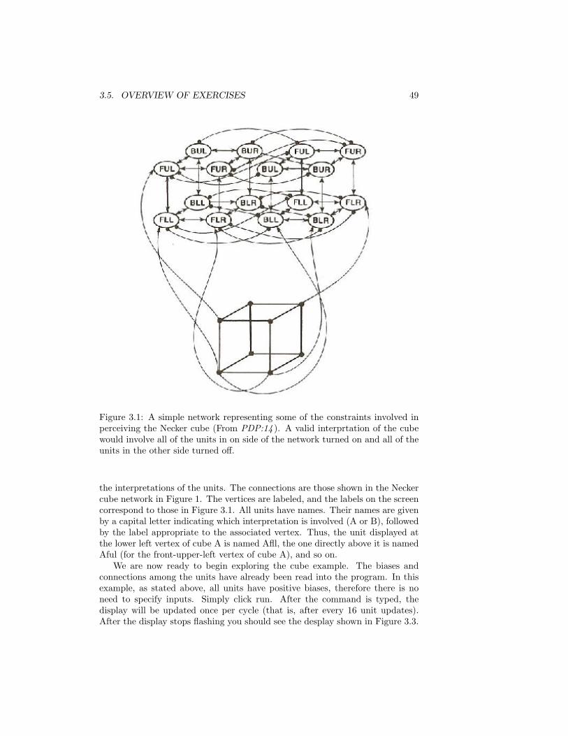
3.5. OVERVIEW OF EXERCISES 49
Figure 3.1: A simple network representing some of the constraints involved inperceiving the Necker cube (From PDP:14 ). A valid interprtation of the cubewould involve all of the units in on side of the network turned on and all of theunits in the other side turned off.
the interpretations of the units. The connections are those shown in the Neckercube network in Figure 1. The vertices are labeled, and the labels on the screencorrespond to those in Figure 3.1. All units have names. Their names are givenby a capital letter indicating which interpretation is involved (A or B), followedby the label appropriate to the associated vertex. Thus, the unit displayed atthe lower left vertex of cube A is named Afll, the one directly above it is namedAful (for the front-upper-left vertex of cube A), and so on.
We are now ready to begin exploring the cube example. The biases andconnections among the units have already been read into the program. In thisexample, as stated above, all units have positive biases, therefore there is noneed to specify inputs. Simply click run. After the command is typed, thedisplay will be updated once per cycle (that is, after every 16 unit updates).After the display stops flashing you should see the desplay shown in Figure 3.3.

50 CHAPTER 3. CONSTRAINT SATISFACTION IN PDP SYSTEMS
Figure 3.2: Initial screen appearance for Cube example.
The variable cycle should be 20, indicating that the program has completed 20cycles. The variable update should be at 16, indicating that we have completedthe 16th update of the cycle. The uname will indicate the last unit updated.The goodness should have a value of 6.4. This value corresponds to a globalmaximum; and indeed, if you inspect the activations, you will see that the unitson the right have reached the maximal value of one, and the units on the left areall 0, corresponding to one of the two “standard” interpretations of the cube.
Q.3.1.1.
Using 3.1, explain quantitatively how the exact value of goodnesscomes to be 6.4 when the network has reached the state shown inthe display. Remember that all weights and biases are scaled by theistr parameter, which is set to .4. Thus each excitatory weight canbe treated as having value .4, each inhibitory weight -.6, and thepositive bias as having value .2.
You can run the cube example again by issuing the newstart command andthen hitting the run button. Do this until you find a case where, after 20 cycles,there are four units on in cube A and four on in cube B. The goodness will be4.8.

3.5. OVERVIEW OF EXERCISES 51
Q.3.1.2.
Using 3.1, explain why the state you have found in this case corre-sponds to a goodness value of 4.8.
Continue again until you find a case where, after 20 cycles, there are twounits on in one of the two cubes and six units on in the other.
Q.3.1.3.
Using Equation 3.1, explain why the state you have found in thiscase also corresponds to a goodness value of 4.8.
Now run about 20 more cases of newstart followed by run, and record for eachthe number of units on in each subnetwork after 20 cycles, making a simple tallyof cases in which the result was [8 0] (all eight units in the left cube activated,none in the right), [6 2], [4 4], [2 6], and [0 8]. Examine the states where thereare units on in both subnetworks.
To facilitate this process, we have provided a little function called onecube(n)that you can execute from the command line. This function issues one newstartand then runs n cycles, showing the final state only. To enter the commandagain, you can use the up-arrow key at the MATLAB command prompt, followedby enter. You can change the value of n by editing the command before you hitenter. For present purposes, you should simply leave n set at 20.
Q.3.1.4.
How many times was each of the two valid interpretations found?How many times did the system settle into a local maximum? Whatwere the local maxima the system found? To what extent do theycorrespond to reasonable interpretations of the cube?
There is a parameter in the schema model, istr, that multiplies the weightsand biases and that, in effect, determines the rate of activation flow within themodel. The probability of finding a local maximum depends on the value of thisparameter. You can set this variable through the value of istr under the optionspopup under the test panel. Another way to set this is by using the commandsettestopts(’istr’,value) where value a positive number. Try several values from0.1 to 2.0, running onecube 20 times for each.
Q.3.1.5.
How does the distribution of final states vary as the value of istris varied? Report your results in table form for each value of istr,showing the number of times the network settles to [8 0], [6 2], [4 4],[2 6], and [0 8] in each case. Consider the distribution of differenttypes of local maxima for different values of istr carefully. Do yourbest explain the results you obtain.

52 CHAPTER 3. CONSTRAINT SATISFACTION IN PDP SYSTEMS
Figure 3.3: The state of the system 20 cycles after the network was initializedat startup.
Hint.
At low values of istr you will want to increase the value of thencycles argument to onecube; 80 works well for values like 0.1. Donot be disturbed by the fact that the values of goodness are differ-ent here than in the previous runs. Since istr effectively scales theweights and biases, it also multiplies the goodness so that goodnessis proportional to istr.
Biasing the necker cube toward one of the two possible solutions. Althoughwe do not provide an excise associated with this, we note that it is possible touse external inputs to bias the network in favor of one of the two interpretations.Study the effects of adding an input of 1.0 to some of the units in one of thesubnetworks, using a command like the following at the command prompt:
net.pools(2).extern_input = [1 1 1 1 1 1 1 1 0 0 0 0 0 0 0 0];
The first eight units are for interpretation A, so this should provide externalinput (scaled by estr, which is set to the same .4 value as istr) to all eight of theunits corresponding to that interpretation. If you wish, you can explore how thedistribution of interpretations changes as a result of varying the number of units

3.6. GOODNESS AND PROBABILITY 53
receiving external input of 1. You can also vary the strength of the externalinputs, either by supplying values different from 1 in the external input vector,or by adjusting the value of the estr parameter.
Schemata for Rooms
One other pre-defined network is available using the schema model. This is anetwork described in PDP:14 that is intended to illustrate various features ofa PDP implementation of the idea of a ’schema’. Consult PDP:14 for a thebackground and for the details of this model.
NOTE: Currently, this example is not working in Version 3.0 of the pdptoolsoftware. Users interested in this example should use software Version 2, andthe earlier version of this handbook.
3.6 GOODNESS AND PROBABILITY
In this section we introduce Hinton and Sejnowski’s Boltzmann machine, de-scribed in PDP:7. This model was developed from an analogy with statisticalphysics and it is useful to put it in this context. We thus begin with a descrip-tion of the physical analogy and then show how this analogy solves some of theproblems of the schema model described above. Then we turn to a descriptionof the Boltzmann machine, show how it is implemented, and allow you to ex-plore how the cs program can be used in boltzmann mode to address constraintsatisfaction problems.
The initial focus of this material when first written in the 1980’s was on theuse of the Boltzmann machine to solve the problem of local minima. However,an alternative, and perhaps more important, perspective on the Boltzmann ma-chine is that is also provides an important step toward a theory of the relation-ship between the content of neural networks (i.e. the knowledge in the weights)and the probability that they settle to particular outcomes. We have alreadytaken a first step in the direction of such a theory, by seeing that networks tendto seek maxima in Goodness, which is in turn related to the knowledge in theweights. In this section we introduce an elegant analysis of the quantitativeform of the relationship between the probability that a network will find itselfin a particular state, and that state’s Goodness. Because of the link betweengoodness and constraints encoded in the weights this analysis allows a deeperunderstanding of the relationship between the constraints and the outcome ofprocessing.
3.6.1 Local Maxima
As stated above, one advantage of the Boltzmann machine over the deterministicconstraint satisfaction system used in the schema model is its ability to overcomethe problem of local maxima in the goodness function. To understand how thisis done, it will be useful to begin with an example of a local maximum and

54 CHAPTER 3. CONSTRAINT SATISFACTION IN PDP SYSTEMS
Figure 3.4: A local maximum found in the schema model.
try to understand in some detail why it occurs and what can be done about it.Figure 3.6.1 illustrates a typical example of a local maximum with the Neckercube. Here we see that the system has settled to a state in which the upperfour vertices were organized according to interpretation A and the lower fourvertices were organized according to interpretation B. Local maxima are alwaysblends of parts of the two global maxima. We never see a final state in whichthe points are scattered randomly across the two interpretations.
All of the local maxima are cases in which one small cluster of adjacentvertices are organized in one way and the rest are organized in another. This isbecause the constraints are local. That is, a given vertex supports and receivessupport from its neighbors. The units in the cluster mutually support oneanother. Moreover, the two clusters are always arranged so that none of theinhibitory connections are active. Note in this case, Afur is on and the two unitsit inhibits, Bfur and Bbur, are both off. Similarly, Abur is on and Bbur andBfur are both off. Clearly the system has found little coalitions of units thathang together and conflict minimally with the other coalitions. In Ex. 3.1, wehad the opportunity to explore the process of settling into one of these localmaxima. What happens is this. First a unit in one subnetwork comes on. Thena unit in the other subnetwork, which does not interact directly with the first, isupdated, and, since it has a positive bias and at that time no conflicting inputs,

3.6. GOODNESS AND PROBABILITY 55
it also comes on. Now the next unit to come on may be a unit that supportseither of the two units already on or possibly another unit that doesn’t interactdirectly with either of the other two units. As more units come on, they willfit into one or another of these two emerging coalitions. Units that are directlyinconsistent with active units will not come on or will come on weakly and thenprobably be turned off again. In short, local maxima occur when units thatdon’t interact directly set up coalitions in both of the subnetworks; by the timeinteraction does occur, it is too late, and the coalitions are set.
Interestingly, the coalitions that get set up in the Necker cube are analogousto the bonding of atoms in a crystalline structure. In a crystal the atoms interactin much the same way as the vertices of our cube. If a particular atom is orientedin a particular way, it will tend to influence the orientation of nearby atoms sothat they fit together optimally. This happens over the entire crystal so thatsome atoms, in one part of the crystal, can form a structure in one orientationwhile atoms in another part of the crystal can form a structure in another ori-entation. The points where these opposing orientations meet constitute flaws inthe crystal. It turns out that there is a strong mathematical similarity betweenour network models and these kinds of processes in physics. Indeed, the workof Hopfield (1982, 1984) on so-called Hopfield nets, of Hinton and Sejnowski(1983), PDP:7, on the Boltzmann machine, and of Smolensky (1983), PDP:6,on harmony theory were strongly inspired by just these kinds of processes. Inphysics, the analogs of the goodness maxima of the above discussion are energyminima. There is a tendency for all physical systems to evolve from highly ener-getic states to states of minimal energy. In 1982, Hopfield, (who is a physicist),observed that symmetric networks using deterministic update rules behave insuch a way as to minimize an overall measure he called energy defined over thewhole network. Hopfield’s energy measure was essentially the negative of ourgoodness measure. We use the term goodness because we think of our systemas a system for maximizing the goodness of fit of the system to a set of con-straints. Hopfield, however, thought in terms of energy, because his networksbehaved very much as thermodynamical systems, which seek minimum energystates. In physics the stable minimum energy states are called attractor states.This analogy of networks falling into energy minima just as physical systemsdo has provided an important conceptual tool for analyzing parallel distributedprocessing mechanisms.
Hopfield’s original networks had a problem with local ”energy minima” thatwas much worse than in the schema model described earlier. His units werebinary. (Hopfield (1984) subsequently proposed a version in which units takeon a continuum of values to help deal with the problem of local minima in hisoriginal model. The schema model is similar to Hopfield’s 1984 model, andwith small values of istr we have seen that it is less likely to settle to a localminimum). For binary units, if the net input to a unit is positive, the unittakes on its maximum value; if it is negative, the unit takes on its minimumvalue (otherwise, it doesn’t change value). Binary units are more prone to localminima because the units do not get an opportunity to communicate with oneanother before committing to one value or the other. In Ex. 3.1, we gave you

56 CHAPTER 3. CONSTRAINT SATISFACTION IN PDP SYSTEMS
the opportunity to run a version close to the binary Hopfield model by settingistr to 2.0 in the Necker cube example. In this case the units are always ateither their maximum or minimum values. Under these conditions, the systemreaches local goodness maxima (energy minima in Hopfield’s terminology) muchmore frequently.
Once the problem has been cast as an energy minimization problem andthe analogy with crystals has been noted, the solution to the problem of localgoodness maxima can be solved in essentially the same way that flaws are dealtwith in crystal formation. One standard method involves annealing. Annealingis a process whereby a material is heated and then cooled very slowly. The ideais that as the material is heated, the bonds among the atoms weaken and theatoms are free to reorient relatively freely. They are in a state of high energy.As the material is cooled, the bonds begin to strengthen, and as the coolingcontinues, the bonds eventually become sufficiently strong that the materialfreezes. If we want to minimize the occurrence of flaws in the material, we mustcool slowly enough so that the effects of one particular coalition of atoms hastime to propagate from neighbor to neighbor throughout the whole materialbefore the material freezes. The cooling must be especially slow as the freezingtemperature is approached. During this period the bonds are quite strong sothat the clusters will hold together, but they are not so strong that atoms inone cluster might not change state so as to line up with those in an adjacentcluster even if it means moving into a momentarily more energetic state. In thisway annealing can move a material toward a global energy minimum.
The solution then is to add an annealing-like process to our network modelsand have them employ a kind of simulated annealing. The basic idea is to adda global parameter analogous to temperature in physical systems and thereforecalled temperature. This parameter should act in such a way as to decrease thestrength of connections at the start and then change so as to strengthen themas the network is settling. Moreover, the system should exhibit some randombehavior so that instead of always moving uphill in goodness space, when thetemperature is high it will sometimes move downhill. This will allow the systemto ”step down from” goodness peaks that are not very high and explore otherparts of the goodness space to find the global peak. This is just what Hinton andSejnowski have proposed in the Boltzmann machine, what Geman and Geman(1984) have proposed in the Gibbs sampler, and what Smolensky has proposedin harmony theory. The essential update rule employed in all of these models isprobabilistic and is given by what we call the logistic function:
p(ai = 1) =eneti/T
eneti/T + 1(3.6)
where T is the temperature. Dividing the numerator and denominator by eneti/T
gives the following version of this function, which is the one must typically used:
p(ai = 1) =1
1 + e−neti/T(3.7)
This differs from the basic schema model in several important ways. First, like

3.6. GOODNESS AND PROBABILITY 57
Hopfield’s original model, the units are binary. They can only take on values of 0and 1. Second, they are stochastic – that is, their value is subject to uncertainty.The update rule specifies only a probability that the units will take on one or theother of their values. This means that the system need not necessarily go uphillin goodness-it can move downhill as well. Third, the behavior of the systemsdepends on a global parameter, T , which determines the relative likelihood ofdifferent states in the network.
In fact, in networks of this type, a very important relationship holds betweenthe equilibrium probability of a state and the state’s goodness:
p(Si) =eGi/T∑i′ e
Gi′/T(3.8)
The denominator of this expression is a sum over all possible states, and is oftendifficult to compute, but we now can see the likelihood ratio of being in eitherof two states S1 or S2 is given by
p(S1)p(S2)
=eG1/T
eG2/T, (3.9)
or alternatively,p(S1)p(S2)
= e(G1−G2)/T . (3.10)
A final way of looking at this relationship that is sometimes useful comes if wetake the log of both sides of this expression:
log(p(S1)p(S2)
) = (G1 −G2)/T. (3.11)
At equilibrium, the log odds of the two states is equal to the difference ingoodness, divided by the temperature.
These simple expressions above can serve two important purposes for neuralnetwork theory. First, they allow us to predict what a network will do fromknowledge of the constraints encoded in its weights, biases, and inputs, whenthe network is run at a fixed temperature. This allows a mathematical derivationof aspects a network’s behavior and it allows us to relate the network’s behaviorto theories of optimal inference.
Second, these expressions allow us to prove that we can, in fact, find a wayto have networks settle to one of their global maxima. In essence, the reason forthis is that, as T grows small, the probability ratios of particular pairs of statesbecome more and more extreme. Consider two states with Goodness 5 andgoodness 4. When T is 1, the ratio of the probabilities is e, or 2.73:1. But whenthe temperature is .1, the ratio e10, or 22,026:1. In general, as temperature goesdown we can make the ratio of the probabilities of two states as large as we like,even if the goodness difference between their probabilities is small.
However, there is one caveat. This is that the above is true, only at equilib-rium, and provided that the system is ergodic.

58 CHAPTER 3. CONSTRAINT SATISFACTION IN PDP SYSTEMS
The equilibrium probability of a state is a slightly tricky concept. It is bestunderstood by thinking of a very large number of copies of the very same net-work, each evolving randomly over time (with a different random seed, so eachone is different). Then we can ask: What fraction of these networks are in anygiven state at any given time? They might all start out in the same state, andthey may all tend to evolve toward better states, but at some point the tendencyto move into a good state is balanced by the tendency to move out of it again,and at this point we say that the probability distribution has reached equilib-rium. At moderate temperatures, the flow between states occurs readily, andthe networks tend to follow the equilibrium distribution at they jump aroundfrom state to state. At low temperatures, however, jumping between statesbecomes very unlikely, and so the networks may be more likely to be found inlocal maxima than in states that are actually better but are also neighbors ofeven better states. When the flow is possible, we say that the system is ergodic.When the system is ergodic, the equilibrium is independent of the starting state.When the flow is not completely open, it is not possible to get from some statesto some other states.
In practice “ergodicity” is a matter of degree. If nearby relatively bad stateshave very low probability of being entered from nearly higher states, it cansimply take more time that it seems practical to wait for much in the way offlow to occur. This is where simulated annealing comes in. We can start withthe temperature high, allowing a lot of flow out of relatively good states andgradually lower the temperature to some desired level. At this temperature, thedistribution of states can in some cases approximate the equilibrium distribu-tion, even though there is not really much ongoing movement between differentstates.
Ex3.2. Exploring Equilibria in the Cube Network
To get a sense of all of this, we will run a few more exercises. Each exercise willinvolve running an ensemble of networks (100 of them) and then looking at thedistribution across states at the end of some number of cycles. Luckily, we areusing a simple network, so running an ensemble of them goes quickly.
To start this exercise, exit from the cube example through the pdp window(so that all your windows close). To make sure everything is cleared up, youcan type
close all; clear all;
at the command prompt. Then start up again using the command cs boltzcubeto the command prompt. What is different about this compared to cube isthat the model is initiated in Boltzmann mode, with an annealing schedulespecified, and both istr and estr are set to 1 so that the goodness values aremore transparent. The two global optima are associated with goodness of 16.This consists of 12 times 1 for the weights along the edges of the interpretationin which all of the units are active, plus 8 times .5 for the bias inputs to the

3.6. GOODNESS AND PROBABILITY 59
eight units representing the corners of that cube. The local maxima we haveconsidered all have goodness of 12.
The annealing schedule is specified at the command prompt via a MATLABcommand. Throughout this exercise, we will work with a final temperature of0.5. The initial annealing schedule is set in the script by the command:
net.schedule = [0 2;20 .5];
This tells the network to initialize the temperature at 2, then linearly reduce itover 20 cycles to .5. In general the schedule consists of a set of time value pairs,separated by a semicolon. Times must increase, and values must be greaterthan 0 (use .001 if you want effectively 0 temperature). Again, though, for ourexercise, we will use a final temperature of .5. After initializing the network,you can explore a few example runs, using the step and/or run command in thetest window. To restart the network click either newstart or reset. As before,reset allows you to repeat an earlier run exactly, while newstart sets the randomnumber seed to a new value so that you will get a statistically independent newrun of the network.
To run an ensemble of networks, you can do so using the manycubes com-mand. Note that this command assumes that you have previously entered thecs boltzcube command, so that the network and display have been initialized.This command takes two arguments. The first is the number of instances of thenetwork settling process to run and the second is the number of cycles to use inrunning each instance. Enter the command shown below now at the commandprompt with arguments 100 and 20, to run 100 instances of the network eachfor 20 cycles.
histvals = manycubes(100,20)
If you have the Network Viewer window open on your screen, you’ll see the initialand final states for each instance of the settling process flash by one by one. Atthe end of 100 instances, a bar graph will pop up, showing the distributionof goodness values of the states reached after 20 cycles. The actual numberscorresponding to the bars on the graph are stored in the histvals variable; thereare 33 values corresponding to goodnesses from 0 to 16 in steps of 0.5. Enterhistvals(17:33) to display the entries corresponding to goodness values from 8to 16. In one run of the manycubes(100,20), the results came out like this:
• 62 states with goodness 16
• 14 states with goodness 13.5
• 2 states with goodness 12.5
• 10 states with goodness 12
We want to know whether we are getting about the right equilibrium dis-tribution of states, given that our final temperature is .5. We can calculate theratios of probabilities of being in particular states, but we need to take into

60 CHAPTER 3. CONSTRAINT SATISFACTION IN PDP SYSTEMS
account that in fact there are several states with each of the four goodness val-ues mentioned above. The probability of having a particular goodness is equalto the probability of being in a particular state with that goodness times thenumber of such states.
Since we need to have the right numbers to proceed, we give the numbers ofsuch states below:
• 2 different states have goodness 16
• 16 different states have goodness 13.5
• 16 different states have goodness 12.5
• 36 different states have goodness 12
The question below asks you to identify the states associated with thesegoodnesses and explain the reasons why they have these goodness values. Ituses a shorthand notation [x y] to represent states with x units on in cube Aand y units on in cube B.
Q.3.2.1.
For the states of goodness 16, we already know that these are theones in which all 8 of the units for one of the cubes in on and noneof the units for the other cube are on, and these states can be called[8 0] and [0 8] states. Now consider the goodness of states close tothe states of goodness 16, but differing from these in the state ofone of the units. Some of these states have goodness of 13.5 andsome have goodness 12.5. Characterize each kind of state, explainwhy there are 16 of each kind, and explain why the Goodness hasthe indicated value.
Consider also the states with goodness 12. There are 36 such states,as indicated. 12 of these are local maxima, but the remaining 24 arenot. Let’s consider first the local maxima. How many of these are[6 2] states? (There is an equal number of [2 6] states. Since theyare analogous to the [2 6] states we will not consider them further).There are many ways to have only 6 units on in cube A and 2 unitson in cube B. State how [6 2] states with goodness 12 differ fromother [6 2] states and explain why they differ in goodness. Similarly,how many states with goodness 12 are [4 4] states? State how thesestates differ from other states in which there are 4 units on in eachcube, and again explain the reason for this difference.
Finally, consider the remaining 24 states with goodness 12. Thesestates correspond to states in which all the units in one cube areactive and both units associated with any single edge of the othercube are active. For one such state, explain why its goodness is 12.Explain why there are 24 such states.
Hint.

3.6. GOODNESS AND PROBABILITY 61
For the second part, refer to the section on local maxima in the firstpart of this chapter for a brief discussion of the goodness 12 states,which correspond to the local maxima.
In any case, with the above information in hand, we can finally ask, whatis the relative probability of being in a state with one of these four goodnesses,given the final temperature achieved in the network?
We can calculate this as follows. For each Goodness Value (GV ), we have:
p(GV ) = NGVe(GV/T )
Z(3.12)
Here NGV represents the number of different states having the goodness valuein question, and e(GV/T ) is proportional to the probability of being in any oneof these states. We use Z to represent the denominator, which we will not needto calculate. Consider first the value of this expression for the highest goodnessvalue, GV = 16, corresponding to the global maxima. There are two such max-ima, so NGV = 2. So to calculate the numerator of this expression (disregardingZ) for our temperature T = .5, we enter the following at or MATLAB commandprompt:
2*exp(16/.5)
We see this is a very large number. To see it in somewhat more compact formatenter format short g at the MATLAB prompt then enter the above expressionagain. The number is 1.58 times 10 to the 14th power. Things come back intoperspective when we look at the ratio of the probability of being in a state withgoodness 16 to the probability of being in a state with goodness 13.5. Thereare 16 such states, so the ratio is given by:
(2*exp(16/.5))/(16*exp(13.5/.5))
The ratio is manageable: it is 18.6 or so. Thus we should have a little morethan 18 times as many states of goodness 16 as we have states of goodness 13.5.In fact we are quite far off from this in my run; we have 62 cases of states ofgoodness 16, and 14 cases of states of goodness 13.5, so the ratio is 4.4 and istoo low.
Q.3.2.2.
Calculate the ratio of the probability of being in a state of goodness16 to the probability of being in a state of goodness 12, taking intoaccount the number of states of each goodness as well as eexp(GV/T )
for each state. Write down all four relevant numbers and calculatethe resulting ratio.
You should obtain a ratio of 165.61. Since I observed 62 states of goodness 16,and 10 of goodness 12, the observed ratio is also off: 62/10 is only 6.2.
Looking at the probability ratio for states of goodness 12.5 vs. 12, we have:
(16*exp(12.5/.5))/(36*exp(12/.5))

62 CHAPTER 3. CONSTRAINT SATISFACTION IN PDP SYSTEMS
The ratio is 1.2. Thus, at equilibrium the network should be in a 12.5 goodnessstate slightly more often than a 12 goodness state. However, we have the oppo-site pattern, with 10 instances of goodness 12 and 2 of goodness 12.5. Clearly,we have not achieved an approximation of the equilibrium distribution; it ap-pears that many instances of the network are stuck in one of the local maxima.Indeed, most of the goodness 12 states are local maxima, while at equilibrium,only 1/3 should be such states.
The approximate expected counts of 100 samples at equilibrium should beas shown below. The next question asks you to try to find an annealing schedulethat will produce a distribution close to the one reported in the table.
Goodness Expected Count per 100 samples16 93.113.5 5.012.5 0.712 0.6All others < 1
Q.3.2.3.
Find an annealing schedule that runs for 50 cycles, has a final tem-perature of 0.5, and ends up as close as possible to the right finaldistribution over the states with goodness values of 16, 13.5, 12.5,and 12. (Some lower goodness values may also appear occasionally.)In particular, try to find a schedule that produces 1 or fewer stateswith a goodness value of 12 per hundred samples. For simplicity,explore only the the starting point and the cycle number at whichyou reach a temperature of .5 (See detailed instructions below). Itis best to do a run of 200 or 500 samples with each schedule to getreasonably stable results. (500 recommended unless your computerturns out to be slow).
Report the results of your best annealing schedule and three thatwere less good in a table, showing the annealing schedules used aswell as the number of states per goodness value (between 8 and 16)at the end of each run. For your best schedule, report the resultsof two runs, since there is variability from run to run. Finally, tryto express a generalization about what makes for a better schedule.See if you can express a hypothesis about why such a schedule worksbetter and do your best to justify your hypothesis.
Detailed Instructions. As stated above, your annealing schedule shouldspecify only an initial temperature and a cycle number (less than or equal to50) at which you will reach the final temperature of .5. An example of such aschedule is shown here:
[0 5; 30 .5];

3.6. GOODNESS AND PROBABILITY 63
This schedule starts at 5 and reaches the final temperature of .5 at cycle 30. Ex-plore values of the starting temperature between .5 and 5 and values of the cyclenumber at which you reach the final temperature between 5 and 50 (of course,if you start at .5, you reach your final temperature at cycle 0). After starting upcs boltzcube you can set net.schedule and then call the manycubes functiondirectly, as in the example below:
net.schedule = [0 5; 30 .5];histvals = manycubes(500,50);
If you do that, the network viewer window will flash up the beginning andending state of each sample. After finishing all the samples, a graph will appearshowing how often the network settled into a state with each of the differentpossible goodness values. The values shown in the histogram will be returned,and we have stored them in an array called histvals. Alternatively, there’s away to run the simulator from a batch file that will not open the gui so that theresults will be computed faster, as described in the next paragraph.We have created a function manycubes batch that takes three arguments, nsam-ples, ncycles, and schedule. To use this function, first close the cs boltzcubenetwork if you had it open, and type ’close all; clear all’. Then call the functionas follows (an example with specific argument values is shown):
histvals = manycubes_batch(500,50,[0 5; 30 .5]); histvals(23:33)/500
This function also displays a histogram of results and returns the array we havestored in ’histvals’ which contains the number of times each of the goodnessvalues was observed across the nsamples different runs. The extra stuff atthe end (after the semicolon) will cause the network to print out the entries inhistvals corresponding to goodness values ranging from 11 (histvals(23)) to 16(histvals(33)). With the given command, 500 samples are run, and the entriesin histvals will appear as percentages, to compare with the numbers in the tableabove. The bar graph that will be shown will make it easy to get a sense ofwhat is going on while the screen dump of the numbers gives you the actualvalues. Giving a different name to the variable I called histvals for each differentannealing schedule you try will allow you to save a separate list of histvals foreach run (make sure to change both occurrances of histvals in the commandabove so that the correct results are displayed to the screen by the second partof the command!)
If you call the above function with several different annealing schedules,then the main MATLAB window will contain a record of all of your annealingschedules and all of your data, and you can copy and paste individual linesinto your homework paper; of course, you will want to edit and reformat forreadability. Remember you can use the arrow keys to access previous commandsand that you can edit them before hitting enter.

64 CHAPTER 3. CONSTRAINT SATISFACTION IN PDP SYSTEMS
3.6.2 Escaping from Local Maxima
The title of this section is a bit of a play on words. We have been focusing onlocal maxima, and how to escape from them, in a way that may distract fromthe deeper contribution of the relationship between goodness and probability.For example, it may be that local maxima are not as much of a problem in PDPsystems as the cube example makes it seem like they might be. The constraintsused in this example were deliberately chosen to create a network that wouldhave such maxima, so that it would help illustrate several useful concepts. Butare local maxima inevitable?
Q.3.2.4.
Consider how you might change the network used in the cube exam-ple to avoid the problem of local maxima. Assume you still have thesame sixteen vertex units, and the same bias inputs making eachof the two interpretations equally likely. Briefly explain (with anoptional drawing) one example in which adding connections wouldhelp and one example in which adding hidden units would help.
Your answer may help to illustrate both that local maxima are not neces-sarily inevitable and that hidden units (units representing important clusters ofinputs that tend to occur together in experience) may play a role in solving thelocal maximum problem. More generally, the point here is to suggest that therelationship between constraints, goodness, and probability may be a useful oneeven beyond avoiding the problem of getting stuck in local maxima.

Chapter 4
Learning in PDP Models:The Pattern Associator
In previous chapters we have seen how PDP models can be used as content-addressable memories and constraint-satisfaction mechanisms. PDP models arealso of interest because of their learning capabilities. They learn, naturally andincrementally, in the course of processing. In this chapter, we will begin toexplore learning in PDP models. We will consider two “classical” proceduresfor learning: the so-called Hebbian, or correlational learning rule, described byHebb (1949) and before him by William James (1950), and the error-correctingor “delta” learning rule, as studied in slightly different forms by Widrow andHoff (1960) and by Rosenblatt (1959).
We will also explore the characteristics of one of the most basic networkarchitectures that has been widely used in distributed memory modeling withthe Hebb rule and the delta rule. This is the pattern associator. The patternassociator has a set of input units connected to a set of output units by a singlelayer of modifiable connections that are suitable for training with the Hebb ruleand the delta rule. Models of this type have been extensively studied by JamesAnderson (see Anderson, 1983), Kohonen (1977), and many others; a number ofthe papers in the Hinton and Anderson (1981) volume describe models of thistype. The models of past-tense learning and of case-role assignment in PDP:18and PDP:19 are pattern associators trained with the delta rule. An analysis ofthe delta rule in pattern associator models is described in PDP:11.
As these works point out, one-layer pattern associators have several sug-gestive properties that have made them attractive as models of learning andmemory. They can learn to act as content-addressable memories; they gener-alize the responses they make to novel inputs that are similar to the inputsthat they have been trained on; they learn to extract the prototype of a set ofrepeated experiences in ways that are very similar to the concept learning char-acteristics seen in human cognitive processes; and they degrade gracefully withdamage and noise. In this chapter our aim is to help you develop a basic un-
65

66CHAPTER 4. LEARNING IN PDP MODELS: THE PATTERN ASSOCIATOR
derstanding of the characteristics of these simple parallel networks. However, itmust be noted that these kinds of networks have limitations. In the next chapterwe will examine these limitations and consider learning procedures that allowthe same positive characteristics of pattern associators to manifest themselvesin networks and overcome one important class of limitations.
We begin this chapter by presenting a basic description of the learning rulesand how they work in training connections coming into a single unit. We willthen apply them to learning in the pattern associator.
4.1 BACKGROUND
4.1.1 The Hebb Rule
In Hebb’s own formulation, this learning rule was described eloquently but onlyin words. He proposed that when one neuron participates in firing another, thestrength of the connection from the first to the second should be increased. Thishas often been simplified to ‘cells that fire together wire together’, and this inturn has often been representated mathematically as:
∆wij = εaiaj (4.1)
Here we use ε to refer to the value of the learning rate parameter. Thisversion has been used extensively in the early work of James Anderson (e.g.,Anderson, 1977). If we start from all-zero weights, then expose the network toa sequence of learning events indexed by l, the value of any weight at the endof a series of learning events will be
wij = ε∑l
ailajl (4.2)
In studying this rule, we will assume that activations are distributed around0 and that the units in the network have activations that can be set in eitherof two ways: They may be clamped to particular values by external inputs orthey may be determined by inputs via their connections to other units in thenetwork. In the latter case, we will initially focus on the case where the unitsare completely linear; that is, on the case in which the activation and the outputof the unit are simply set equal to the net input:
ai =∑j
ajwij (4.3)
In this formulation, with the activations distributed around 0, the wij as-signed by Equation 4.2 will be proportional to the correlation between the acti-vations of units i and j; normalizations can be used to preserve this correlationalproperty when units have mean activations that vary from 0.
The correlational character of the Hebbian learning rule is at once thestrength of the procedure and its weakness. It is a strength because these

4.1. BACKGROUND 67
Figure 4.1: Two simple associative networks and the patterns used in trainingthem.
correlations can sometimes produce useful associative learning; that is, partic-ular units, when active, will tend to excite other units whose activations havebeen correlated with them in the past. It can be a weakness, though, sincecorrelations between unit activations often are not sufficient to allow a networkto learn even very simple associations between patterns of activation.
First let’s examine a positive case: a simple network consisting of two inputunits and one output unit (Figure 4.1A). Suppose that we arrange things sothat by means of inputs external to this network we are able to impose patternsof activation on these units, and suppose that we use the Hebb rule (Equation4.1 above) to train the connections from the two input units to the output unit.Suppose further that we use the four patterns shown in Figure 4.1B; that is, wepresent each pattern, forcing the units to the correct activation, then we adjustthe strengths of the connections between the units. According to Equation 4.1,w20 (the weight on the connection to unit 2 from unit 0) will be increased instrength for each pattern by amount ε, which in this case we will set to 1.0. Onthe other hand, w21 will be increased by amount ε in two of the cases (first andlast pattern) and reduced by ε in the other cases, for a net change of 0.

68CHAPTER 4. LEARNING IN PDP MODELS: THE PATTERN ASSOCIATOR
As a result of this training, then, this simple network would have acquireda positive connection weight to unit 2 from unit 0. This connection will nowallow unit 0 to make unit 2 take on an activation value correlated with that ofunit 0. At the same time, the network would have acquired a null connectionfrom unit 1 to unit 2, capturing the fact that the activation of unit 1 has nopredictive relation to the activation of unit 2. In this way, it is possible to useHebbian learning to learn associations that depend on the correlation betweenactivations of units in a network.
Unfortunately, the correlational learning that is possible with a Hebbianlearning rule is a “unitwise” correlation, and sometimes, these unitwise cor-relations are not sufficient to learn correct associations between whole inputpatterns and appropriate responses. To see that this is so, suppose we changeour network so that there are now four input units and one output unit, asshown in Figure 4.1C. And suppose we want to train the connections in thenetwork so that the output unit takes on the values given in Figure 4.1D foreach of the four input patterns shown there. In this case, the Hebbian learningprocedure will not produce correct results. To see why, we need to examine thevalues of the weights (equivalently, the pairwise correlations of the activationsof each sending unit with the receiving unit). What we see is that three of theconnections end up with 0 weights because the activation of the correspondinginput unit is uncorrelated with the activation of the output unit. Only one ofthe input units, unit 2, has a positive correlation with unit 4 over this set ofpatterns. This means that the output unit will make the same response to thefirst three patterns since in all three of these cases the third unit is on, and thisis the only unit with a nonzero connection to the output unit.
Before leaving this example, we should note that there are values of theconnection strengths that will do the job. One such set is shown in Figure 4.1E.The reader can check that this set produces the correct results for each of thefour input patterns by using Equation 4.3.
Apparently, then, successful learning may require finding connection strengthsthat are not proportional to the correlations of activations of the units. Howcan this be done?
4.1.2 The Delta Rule
One answer that has occurred to many people over the years is the idea of usingthe difference between the desired, or target, activation and the obtained activa-tion to drive learning. The idea is to adjust the strengths of the connections sothat they will tend to reduce this difference or error measure. Because the ruleis driven by differences, we have tended to call it the delta rule. Others havecalled it the Widrow-Hoff learning rule or the least mean square (LMS) rule(Widrow and Hoff, 1960); it is related to the perceptron convergence procedureof Rosenblatt (1959).
This learning rule, in its simplest form, can be written
∆wij = εeiaj (4.4)
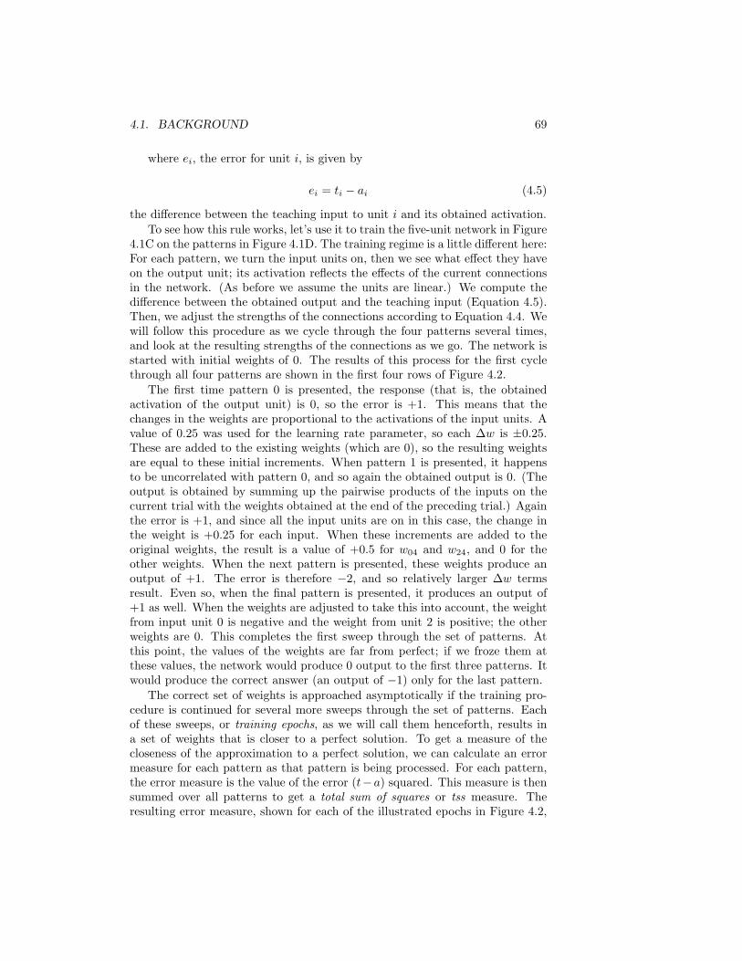
4.1. BACKGROUND 69
where ei, the error for unit i, is given by
ei = ti − ai (4.5)
the difference between the teaching input to unit i and its obtained activation.To see how this rule works, let’s use it to train the five-unit network in Figure
4.1C on the patterns in Figure 4.1D. The training regime is a little different here:For each pattern, we turn the input units on, then we see what effect they haveon the output unit; its activation reflects the effects of the current connectionsin the network. (As before we assume the units are linear.) We compute thedifference between the obtained output and the teaching input (Equation 4.5).Then, we adjust the strengths of the connections according to Equation 4.4. Wewill follow this procedure as we cycle through the four patterns several times,and look at the resulting strengths of the connections as we go. The network isstarted with initial weights of 0. The results of this process for the first cyclethrough all four patterns are shown in the first four rows of Figure 4.2.
The first time pattern 0 is presented, the response (that is, the obtainedactivation of the output unit) is 0, so the error is +1. This means that thechanges in the weights are proportional to the activations of the input units. Avalue of 0.25 was used for the learning rate parameter, so each ∆w is ±0.25.These are added to the existing weights (which are 0), so the resulting weightsare equal to these initial increments. When pattern 1 is presented, it happensto be uncorrelated with pattern 0, and so again the obtained output is 0. (Theoutput is obtained by summing up the pairwise products of the inputs on thecurrent trial with the weights obtained at the end of the preceding trial.) Againthe error is +1, and since all the input units are on in this case, the change inthe weight is +0.25 for each input. When these increments are added to theoriginal weights, the result is a value of +0.5 for w04 and w24, and 0 for theother weights. When the next pattern is presented, these weights produce anoutput of +1. The error is therefore −2, and so relatively larger ∆w termsresult. Even so, when the final pattern is presented, it produces an output of+1 as well. When the weights are adjusted to take this into account, the weightfrom input unit 0 is negative and the weight from unit 2 is positive; the otherweights are 0. This completes the first sweep through the set of patterns. Atthis point, the values of the weights are far from perfect; if we froze them atthese values, the network would produce 0 output to the first three patterns. Itwould produce the correct answer (an output of −1) only for the last pattern.
The correct set of weights is approached asymptotically if the training pro-cedure is continued for several more sweeps through the set of patterns. Eachof these sweeps, or training epochs, as we will call them henceforth, results ina set of weights that is closer to a perfect solution. To get a measure of thecloseness of the approximation to a perfect solution, we can calculate an errormeasure for each pattern as that pattern is being processed. For each pattern,the error measure is the value of the error (t−a) squared. This measure is thensummed over all patterns to get a total sum of squares or tss measure. Theresulting error measure, shown for each of the illustrated epochs in Figure 4.2,
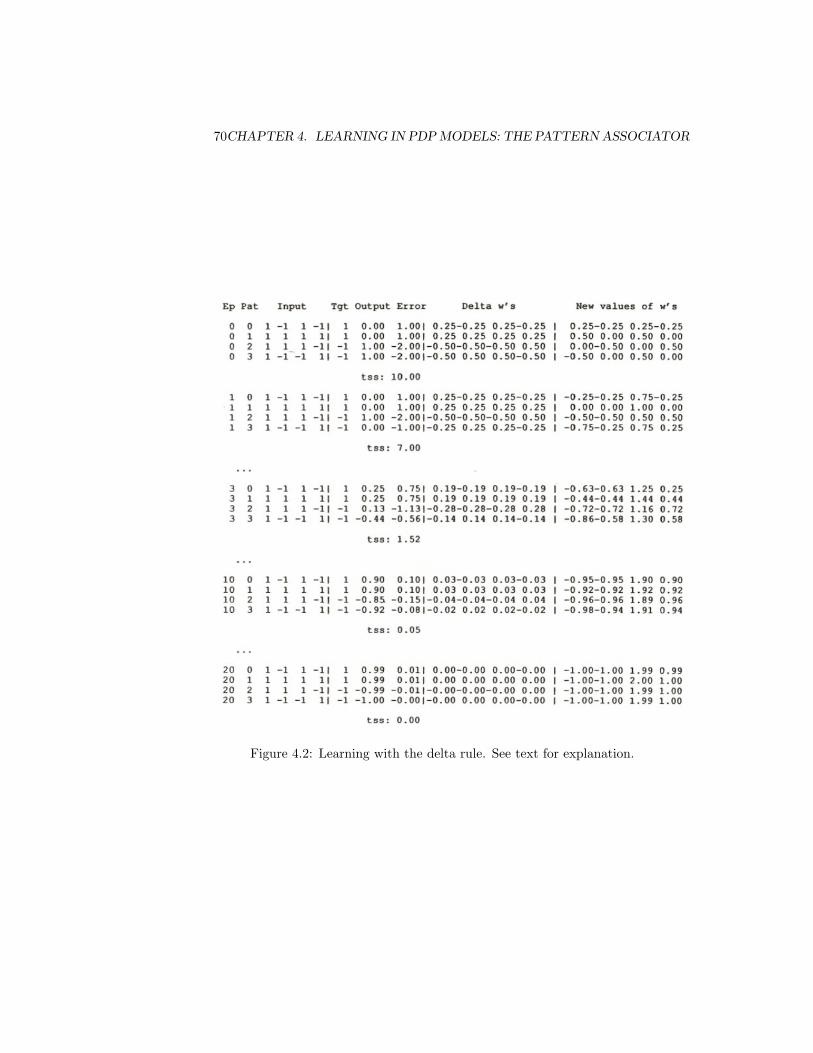
70CHAPTER 4. LEARNING IN PDP MODELS: THE PATTERN ASSOCIATOR
Figure 4.2: Learning with the delta rule. See text for explanation.
4.1. BACKGROUND 71
gets smaller over epochs, as do the changes in the strengths of the connections.The weights that result at the end of 20 epochs of training are very close tothe perfect solution values. With more training, the weights converge to thesevalues.
The error-correcting learning rule, then, is much more powerful than theHebb rule. In fact, it can be proven rather easily that the error-correcting rulewill find a set of weights that drives the error as close to 0 as we want for eachand every pattern in the training set, provided such a set of weights exists.Many proofs of this theorem have been given; a particularly clear one may befound in Minsky and Papert (1969) (one such proof may be found in PDP:11 ).
4.1.3 Division of Labor in Error Correcting Learning
It is worth noting an interesting characteristic of error correcting learning rules.This is that, when possible, they divide up the work of driving output unitsto their correct target values. A simple case of this could arise in the simplenetwork we have already been considering.
Suppose we create a very simple training set consisting of two input patternsand corresponding single desired outputs:
input output+ + + + +- - - + -
In this case, we see that three of the input units are perfectly correlated with theoutput and one is uncorrelated with it. If we present these two input patternsrepeatedly with a small learning rate, the connection weights will converge to
1/3 1/3 1/3 0
You can verify that with these connection weights, the network will produce thecorrect output for both inputs. Now, consider what would happen if the inputpatterns were:
input output+ + + + +- + + + -
Here, only one input unit is correlated with the output unit. What will theconnection weights converge to in this case? The second, third, and fourthunit cannot help predict the output, so these weights will all be 0. The firstunit will have to do all the work, and so the first weight will be 1. Whilethis set of weights would work for the first set of input patterns, the learningrule tends to spread the responsibility or divide the labor among the units thatbest predict the output. This tendency to ’divide the labor’ among the inputunits is a characteristic of error correcting learning, and does not occur withthe simple Hebbian learning rule because that rule is only sensitive to pairwiseinput-output correlations.

72CHAPTER 4. LEARNING IN PDP MODELS: THE PATTERN ASSOCIATOR
4.1.4 The Linear Predictability Constraint
We have just noted that the delta rule will find a set of weights that solves anetwork learning problem, provided such a set of weights exists. What are theconditions under which such a set actually does exist?
Such a set of weights exists only if for each input-pattern-target-pair thetarget can be predicted from a weighted sum, or linear combination, of theactivations of the input units. That is, the set of weights must satisfy
tip =∑j
wijajp (4.6)
for output unit i in all patterns p.This constraint (which we called the linear predictability constraint in PDP:17 )
can be overcome by the use of hidden units, but hidden units cannot be trainedusing the delta rule as we have described it here because (by definition) there isno teacher for them. Procedures for training such units are discussed in Chapter5.
Up to this point, we have considered the use of the Hebb rule and the deltarule for training connections coming into a single unit. We now consider howthese learning rules produce the characteristics of pattern associator networks.
4.2 THE PATTERN ASSOCIATOR
In a pattern associator, there are two sets of units: input units and outputunits. There is also a matrix representing the connections from the input unitsto the output units. A pattern associator is really just an extension of the simplenetworks we have been considering up to now, in which the number of outputunits is greater than one and each input unit has a connection to each outputunit. An example of an eight-unit by eight-unit pattern associator is shown inFigure 4.3.
The pattern associator is a device that learns associations between inputpatterns and output patterns. It is interesting because what it learns about onepattern tends to generalize to other similar patterns. In what follows we willsee how this property arises, first in the simplest possible pattern associator: apattern associator consisting of linear units, trained by the Hebb rule.1
4.2.1 The Hebb Rule in Pattern Associator Models
To begin, let us consider the effects of training a network with a single learningtrial l, involving an input pattern il, and an output pattern ol. We will use thenotational convention that vector names are bolded.
1Readers who wish to gain a better grasp on the mathematical basis of this class of modelsmay find it worthwhile to read PDP:9. An in-depth analysis of the delta rule in patternassociators is in PDP:11.

4.2. THE PATTERN ASSOCIATOR 73
Figure 4.3: A schematic diagram of an eight-unit pattern associator. An inputpattern, an output pattern, and values for the weights that will allow the inputto produce the output are shown. (From PDP:18, p. 227.)

74CHAPTER 4. LEARNING IN PDP MODELS: THE PATTERN ASSOCIATOR
Assuming all the weights in the network are initially 0, we can express thevalue of each weight as
wij = εijloil (4.7)
Note that we are using the variable ijl to stand for the activation of input unit jin input pattern il, and we are using oil to stand for the activation of output uniti in output pattern ol. Thus, each weight is just the product of the activationof the input unit times the activation of the output unit in the learning trial l.
In this chapter, many of the formulas are also presented as MATLAB rou-tines to further familiarize the reader with the MATLAB operations. In theseroutines, the subscript on the vector names will be dropped when clear. Thus,il will just be denoted i in the code. Vectors are assumed to be row vectors.
In MATLAB, the above formula (Eq. 4.7) is an outer product:
W = epsilon * (o’ * i);
where the prime is the transpose operator. Dimensions of the outer product arethe outer dimensions of the contributing vectors: o′ dims are [8 1], i dims are [18], and so W dims are [8 8]. We also adopt the convention that weight matricesare of size [noutputs ninputs].
Now let us present a test input pattern, it, and examine the resulting outputpattern it produces. Since the units are linear, the activation of output unit iwhen tested with input pattern it is
oit =∑j
wijijt (4.8)
which is equivalent to
o = W * i’;
in MATLAB, where o is a column vector. Substituting for wij from Equation4.7 yields
oit =∑j
εijloilijt (4.9)
Since we are summing with respect to j in this last equation, we can pull out εand oil:
oit = εoil∑j
ijlijt (4.10)
Equation 4.10 says that the output at the time of test will be proportional tothe output at the time of learning times the sum of the elements of the inputpattern at the time of learning, each multiplied by the corresponding elementof the input pattern at the time of test.
This sum of products of corresponding elements is called the dot product.It is very important to our analysis because it expresses the similarity of thetwo patterns il and it. It is worth noting that we have already encounteredan expression similar to this one in Equation 4.2. In that case, though, the

4.2. THE PATTERN ASSOCIATOR 75
quantity was proportional to the correlation of the activations of two unitsacross an ensemble of patterns. Here, it is proportional to the correlation of twopatterns across an ensemble of units. It is often convenient to normalize the dotproduct by taking out the effects of the number of elements in the vectors inquestion by dividing the dot product by the number of elements. We will callthis quantity the normalized dot product. For patterns consisting of all +1s and−1s, it corresponds to the correlation between the two patterns. The normalizeddot product has a value of 1 if the patterns are identical, a value of −1 if theyare exactly opposite to each other, and a value of 0 if the elements of one vectorare completely uncorrelated with the elements of the other. To compute thenormalized dot product with MATLAB:
ndp = sum(a.*b)/length(a);
or for two row vectors
ndp = (a*b’)/length(a);
We can rewrite Equation 4.10, then, replacing the summed quantity by thenormalized dot product of input pattern il and input pattern it, which wedenote by (il · it)n:
oit = koil(il · it)n (4.11)
where k = nε (n is the number of units). Since Equation 4.11 applies to all ofthe elements of the output pattern ot, we can write
ot = kol(il · it)n (4.12)
In MATLAB, this is
ot = k * ol * sum(it .* il) / length(it);
This result is very basic to thinking in terms of patterns since it demonstratesthat what is crucial for the performance of the network is the similarity relationsamong the input patterns–their correlations–rather than their specific propertiesconsidered as individuals.2 Thus Equation 4.12 says that the output patternproduced by our network at test is a scaled version of the pattern stored on thelearning trial. The magnitude of the pattern is proportional to the similarity ofthe learning and test patterns. In particular, if k = 1 and if the test pattern isidentical to the training pattern, then the output at test will be identical to theoutput at learning.
An interesting special case occurs when the normalized dot product betweenthe learned pattern and the test pattern is 0. In this case, the output is 0:There is no response whatever. Patterns that have this property are calledorthogonal or uncorrelated ; note that this is not the same as being opposite oranticorrelated.
2Technically, performance depends on the similarity relations among the patterns and ontheir overall strength or magnitude. However, among vectors of equal strength (e.g., thevectors consisting of all +1s and −1s), only the similarity relations are important.

76CHAPTER 4. LEARNING IN PDP MODELS: THE PATTERN ASSOCIATOR
To develop intuitions about orthogonality, you should compute the normal-ized dot products of each of the patterns b, c, d, and e below with patterna:
a = [ 1 1 -1 -1]b = [ 1 -1 1 -1]c = [ 1 -1 -1 1]d = [ 1 1 1 1]e = [-1 -1 1 1]
ndp_ab = sum(a.*b)/length(a);
You will see that patterns b, c, and d are all orthogonal to pattern a; infact, they are all orthogonal to each other. Pattern e, on the other hand, is notorthogonal to pattern a, but is anticorrelated with it. Interestingly, it formsan orthogonal set with patterns b, c, and d. When all the members of a set ofpatterns are orthogonal to each other, we call them an orthogonal set.
Now let us consider what happens when an entire ensemble of patterns ispresented during learning. In the Hebbian learning situation, the set of weightsresulting from an ensemble of patterns is just the sum of the sets of weightsresulting from each individual pattern. Note that, in the model we are con-sidering, the output pattern, when provided, is always thought of as clampingthe state the output units to the indicated values, so that the existing values ofthe weights actually play no role in setting the activations of the output units.Given this, after learning trials on a set of input patterns il each paired withan output pattern ol, the value of each weight will be
wij = ε∑l
ijloil (4.13)
Thus, the output produced by each test pattern is
ot = k∑l
ol(il · it)n (4.14)
In words, the output of the network in response to input pattern t is the sumof the output patterns that occurred during learning, with each pattern’s con-tribution weighted by the similarity of the corresponding input pattern to thetest pattern. Three important facts follow from this:
1. If a test input pattern is orthogonal to all training input patterns, theoutput of the network will be 0; there will be no response to an inputpattern that is completely orthogonal to all of the input patterns thatoccurred during learning.
2. If a test input pattern is similar to one of the learned input patternsand is uncorrelated with all the others, then the test output will be ascaled version of the output pattern that was paired with the similar inputpattern during learning. The magnitude of the output will be proportionalto the similarity of the test input pattern to the learned input pattern.

4.2. THE PATTERN ASSOCIATOR 77
3. For other test input patterns, the output will always be a blend of thetraining outputs, with the contribution of each output pattern weightedby the similarity of the corresponding input pattern to the test inputpattern.
In the exercises, we will see how these properties lead to several desirablefeatures of pattern associator networks, particularly their ability to generalizebased on similarity between test patterns and patterns presented during train-ing.
These properties also reflect the limitations of the Hebbian learning rule;when the input patterns used in training the network do not form an orthogonalset, it is not in general possible to avoid contamination, or “cross-talk,” betweenthe response that is appropriate to one pattern and the response that occurs tothe others. This accounts for the failure of Hebbian learning with the secondset of training patterns considered in Figure 4.1. The reader can check that theinput patterns we used in our first training example in Figure 4.1 (which wassuccessful) were orthogonal but that the patterns used in the second examplewere not orthogonal.
4.2.2 The Delta Rule in Pattern Associator Models
Once again, the delta rule allows us to overcome the orthogonality limitationimposed by the Hebb rule. For the pattern associator case, the delta rule for aparticular input-target pair il, tl is
∆wij = ε(til − oil)ijl. (4.15)
which in MATLAB is (again, assuming row vectors)
delta_w = epsilon * (t-o)’ * i;
Therefore the weights that result from an ensemble of learning pairs indexed byl can be written:
wij = ε∑l
(til − oil)ijl (4.16)
It is interesting to compare this to the Hebb rule. Consider first the casewhere each of the learned patterns is orthogonal to every other one and ispresented exactly once during learning. Then ol will be 0 (a vector of all zeros)for all learned patterns l, and the above formula reduces to
wij = ε∑l
tilijl (4.17)
In this case, the delta rule produces the same results as the Hebb rule; theteaching input simply replaces the output pattern from Equation 4.13. As longas the patterns remain orthogonal to each other, there will be no cross-talkbetween patterns. Learning will proceed independently for each pattern. Thereis one difference, however. If we continue learning beyond a single epoch, the

78CHAPTER 4. LEARNING IN PDP MODELS: THE PATTERN ASSOCIATOR
delta rule will stop learning when the weights are such that they allow thenetwork to produce the target patterns exactly. In the Hebb rule, the weightswill grow linearly with each presentation of the set of patterns, getting strongerwithout bound.
In the case where the input patterns il, are not orthogonal, the results of thetwo learning procedures are more distinct. In this case, though, we can observethe following interesting fact: We can read Equation 4.15 as indicating that thechange in the weights that occurs on a learning trial is storing an association ofthe input pattern with the error pattern; that is, we are adding to each weightan increment that can be thought of as an association between the error forthe output unit and the activation of the input unit. To see the implicationsof this, let’s examine the effects of a learning trial with input pattern il pairedwith output pattern tl on the output produced by test pattern it. The effect ofthe change in the weights due to this learning trial (as given by Equation 4.15)will be to change the output of some output unit i by an amount proportionalto the error that occurred for that unit on the learning trial, ei, times the dotproduct of the learned pattern with the test pattern:
∆oit = keil(il · it)n
Here k is again equal to ε times the number of input units n. In vector notation,the change in the output pattern ot can be expressed as
∆ot = kel(il · it)n
Thus, the change in the output pattern at test is proportional to the errorvector times the normalized dot product of the input pattern that occurredduring learning and the input pattern that occurred during test. Two factsfollow from this:
1. If the input on the learning trial is identical to the input on the test trialso that the normalized dot product is 1.0 and if k = 1.0, then the changein the output pattern will be exactly equal to the error pattern. Sincethe error pattern is equal to the difference between the target and theobtained output on the learning trial, this amounts to one trial learningof the desired association between the input pattern on the training trialand the target on this trial.
2. However, if it is different from il but not completely different so that(il · it)n n is not equal to either 1 or 0, then the output produced by it
will be affected by the learning trial. The magnitude of the effect will beproportional to the magnitude of (il · it)n.
The second effect–the transfer from learning one pattern to performance onanother–may be either beneficial or interfering. Importantly, for patterns of all+1s and −1s, the transfer is always less than the effect on the pattern usedon the learning trial itself, since the normalized dot product of two differentpatterns must be less than the normalized dot product of a pattern with itself.This fact plays a role in several proofs concerning the convergence of the deltarule learning procedure (see Kohonen, 1977, and PDP:11 for further discussion).

4.2. THE PATTERN ASSOCIATOR 79
4.2.3 Linear Predictability and the Linear IndependenceRequirement
Earlier we considered the linear predictability constraint for training a singleoutput unit. Since the pattern associator can be viewed as a collection of sev-eral different output units, the constraint applies to each unit in the patternassociator. Thus, to master a set of patterns there must exist a set of weightswij such that
tip =∑j
wijijp (4.18)
for all output units i for all target-input pattern pairs p. A consequence of thisconstraint for the sets of input-output patterns that can be learned by a patternassociator is something we will call the linear independence requirement :
An arbitrary output pattern op can be correctly associated witha particular input pattern ip without ruining associations betweenother input-output pairs, only if ip is linearly independent of all ofthe other patterns in the training set, that is, as long as ip cannotbe written as a linear combination of the other input patterns.
If pattern ip can be written as a linear combination of the other input patterns,then the output for ip will be a linear combination of the outputs produced bythe other patterns (each other pattern’s contribution to the linear combinationwill be weighted by it’s similarity to ip). If this linear combination just happensto be the correct output for ip, then all is well, but if it is not, the weights willbe changed by the delta rule, and this will distort the output pattern producedby one or more of the other patterns in the set.
A pattern that cannot be written as a linear combination of a set of otherpatterns is said to be linearly independent from these other patterns. When allthe members of a set of patterns are linearly independent, we say they forma linearly independent set. To ensure that arbitrary associations to each of aset of input patterns can be learned, the input patterns must form a linearlyindependent set.
Although this is a serious limitation on what a network can learn, it is worthnoting that there are cases in which the response that we need to make to oneinput pattern can be predictable from the responses that we make to otherpatterns with which they overlap. In these cases, the fact that the patternassociator produces a response that is a combination of the responses to otherpatterns can allow it to produce very efficient, often rule-like solutions to theproblem of mapping each of a set of input patterns to the appropriate response.We will examine this property of pattern associators in the exercises.
4.2.4 Nonlinear Pattern Associators
Not all pattern associator models that have been studied in the literature makeuse of the linear activation assumptions we have been using in this analysis.

80CHAPTER 4. LEARNING IN PDP MODELS: THE PATTERN ASSOCIATOR
Several different kinds of nonlinear pattern associators (i.e., associators in whichthe output units have nonlinear activation functions) fall within the general classof pattern associator models. These nonlinearities have effects on performance,but the basic principles that we have observed here are preserved even whenthese nonlinearities are in place. In particular:
1. Orthogonal inputs are mutually transparent.
2. The learning process converges with the delta rule as long as there is a setof weights that will solve the learning problem.
3. A set of weights that will solve the problem does not always exist.
4. What is learned about one pattern tends to transfer to others.
4.3 THE FAMILY OF PATTERN ASSOCIA-TOR MODELS
With the above as background, we turn to a brief specification of several mem-bers of the class of pattern associator models that are available through the paprogram. These are all variants on the pattern associator theme. Each modelconsists of a set of input units and a set of output units. The activations of theinput units are clamped by externally supplied input patterns. The activationsof the output units are determined in a single two-phase processing cycle. First,the net input to each output unit is computed. This is the sum of the activationsof the input units times the corresponding weights, plus an optional bias termassociated with the output unit:
neti =∑j
wijaj + biasi (4.19)
4.3.1 Activation Functions
After computing the net input to each output unit, the activation of the outputunit is then determined according to an activation function. Several variantsare available:
• Linear. Here the activation of output unit i is simply equal to the netinput.
• Linear threshold. In this variant, each of the output units is a linearthreshold unit ; that is, its activation is set to 1 if its net input exceeds 0and is set to 0 otherwise. Units of this kind were used by Rosenblatt inhis work on the perceptron 1959.
• Stochastic. This is the activation function used in PDP:18 and PDP:19.Here, the output is set to 1, with a probability p given by the logistic

4.3. THE FAMILY OF PATTERN ASSOCIATOR MODELS 81
function:
p(oi = 1) =1
1 + e−neti/T(4.20)
This is the same activation function used in Boltzmann machines.
• Continuous sigmoid. In this variant, each of the output units takes on anactivation that is nonlinearly related to its input according to the logisticfunction:
oi =1
1 + e−neti/T(4.21)
Note that this is a continuous function that transforms net inputs between+∞ and −∞ into real numbers between 0 and 1. This is the activationfunction used in the backpropagation networks we will study in Chapter5.
4.3.2 Learning Assumptions
Two different learning rules are available in the pa program:
• The Hebb rule. Hebbian learning in the pattern associator model worksas follows. Activations of input units are clamped based on an externallysupplied input pattern, and activations of the output units are clampedto the values given by some externally supplied target pattern. Learningthen occurs by adjusting the strengths of the connections according to theHebbian rule:
∆wij = εoiij (4.22)
• The delta rule. Error-correcting learning in the pattern associator modelworks as follows. Activations of input units are clamped to values de-termined by an externally supplied input pattern, and activations of theoutput units are calculated as described earlier. The difference betweenthe obtained activation of the output units and the target activation, asspecified in an externally supplied target pattern, is then used in changingthe weights according to the following formula:
∆wij = ε(ti − oi)ij (4.23)
4.3.3 The Environment and the Training Epoch
In the pattern associator models, there is a notion of an environment of patternpairs. Each pair consists of an input pattern and a corresponding output pat-tern. A training epoch consists of one learning trial on each pattern pair in theenvironment. On each trial, the input is presented, the corresponding outputis computed, and the weights are updated. Patterns may be presented in fixedsequential order or in permuted order within each epoch.

82CHAPTER 4. LEARNING IN PDP MODELS: THE PATTERN ASSOCIATOR
4.3.4 Performance Measures
After processing each pattern, several measures of the output that is producedand its relation to the target are computed. One of these is the normalizeddot product of the output pattern with the target. This measure is called thendp. We have already described this measure quantitatively; here we note thatit gives a kind of combined indication of the similarity of two patterns andtheir magnitudes. In the cases where this measure is most useful-where thetarget is a pattern of +1s and −1s–the magnitude of the target is fixed and thenormalized dot product varies with the similarity of the output to the target andthe magnitude of the output itself. To unconfound these factors, we provide twofurther measures: the normalized vector length, or nvl, of the output vector andthe vector correlation, or vcor, of the output vector with the target vector. Thenvl measures the magnitude of the output vector, normalizing for the numberof elements in the vector. It has a value of 1.0 for vectors consisting of all +1sand −1s. The vcor measures the similarity of the vectors independent of theirlength; it has a value of 1.0 for vectors that are perfectly correlated, 0.0 fororthogonal vectors, and −1.0 for anticorrelated vectors.
Quantitative definitions of vector length and vector correlation are given inPDP:9 (pp. 376-379). The vector length of vector v, ||v||, is the square root ofthe dot product of a vector with itself:
||v|| =√
v · v
and the vector correlation (also called the cosine of the angle between two vec-tors) is the dot product of the two vectors divided by the product of theirlengths:
vcor(u,v) =(u · v)||u|| ||v||
The normalized vector length is obtained by dividing the length by the squareroot of number of elements. Given these definitions, we can now consider therelationships between the various measures. When the target pattern consists of+1s and −1s, the normalized dot product of the output pattern and the targetpattern is equal to the normalized vector length of the output pattern times thevector correlation of the output pattern and the target:
ndp = nvl · vcor. (4.24)
In addition to these measures, we also compute the pattern sum of squaresor pss and the total sum of squares or tss. The pss is the sum over all outputunits of the squared error, where the error for each output unit is the differencebetween the target and the obtained activation of the unit. This quantity iscomputed for each pattern processed. The tss is just the sum over the pssvalues computed for each pattern in the training set. These measures are notvery meaningful when learning occurs by the Hebb rule, but they are meaningfulwhen learning occurs by the delta rule.

4.4. IMPLEMENTATION 83
4.4 IMPLEMENTATION
The pa program implements the pattern associator models in a very straight-forward way. The program is initialized by defining a network, as in previouschapters. A PA network consists of a pool of input units (pools(2)) and a poolof output units (pools(3)). pools(1) contains the bias unit which is always onbut is not used in these exercises. Connections are allowed from input units tooutput units only. The network specification file (pa.net) defines the number ofinput units and output units, as well as the total number of units, and indicateswhich connections exist. It is also generally necessary to read in a file specifyingthe set of pattern pairs that make up the environment of the model.
Once the program is initialized, learning occurs through calls to a routinecalled train. This routine carries out nepochs of training, where the trainingmode can be selected in the Train options window. strain (’s’) trains the networkwith patterns in sequential order, while ptrain (’p’) permutes the order. Thenumber of epochs can also be set in that window. The routine exits if the totalsum of squares measure, tss, is less than some criterion value, ecrit which canalso be set in Train options. Here is the train routine:
function train()epoch_limit = (floor(obj.epochno/obj.train_options.nepochs)+1)*obj.train_options.nepochs;while obj.next_epochno <= epoch_limit
obj.epochno = obj.next_epochno;while obj.next_patno <= length(obj.environment.sequences)
obj.patno = obj.next_patno;obj.environment.sequence_index = obj.patno;obj.clamp_pools;obj.compute_output;obj.compute_error;obj.sumstats;obj.compute_weds;if strcmpi(obj.train_options.lgrain,’pattern’)
obj.change_weights;endobj.next_patno = obj.patno + 1;if obj.done_updating_patno
returnend
endif strcmpi(obj.train_options.lgrain,’epoch’)
obj.change_weights;endobj.next_patno = 1;obj.epochno = obj.next_epochno;obj.next_epochno = obj.next_epochno + 1;if obj.done_updating_epochno

84CHAPTER 4. LEARNING IN PDP MODELS: THE PATTERN ASSOCIATOR
returnend
end
This calls four other routines: one that sets the input pattern (clamp pools),one that computes the activations of the output units from the activations ofthe input units (compute output), one that computes the error measure (com-pute error), and one that computes the various summary statistics (sumstats).
Below we show the compute output and the compute error routines. First,compute output :
function compute_output(pattern,patnum,opts)[obj.pools([obj.pools.clamped_activation] ~= 2).activation] =obj.pools([obj.pools.clamped_activation] ~= 2).activation_reset_value;[obj.pools.net_input] = obj.pools.net_input_reset_value;for i=1:numel(obj.pools)
if obj.pools(i).clamped_activation == 2continue
endfor j=1:length(obj.pools(i).projections)
from = obj.pools(i).projections(j).from;obj.pools(i).net_input = obj.pools(i).net_input + (from.activation *obj.pools(i).projections(j).using.weights’);
endswitch obj.pools(i).activation_function
case ’logistic’obj.pools(i).activation = obj.pools(i).activation + logistic(obj.pools(i).net_input);
case ’linear’obj.pools(i).activation = obj.pools(i).net_input;
case ’stochastic’logout = logistic(obj.pools(i).net_input ./ obj.temp);r = rand(1,numel(logout));obj.pools(i).activation(r < logout) = 1.0;obj.pools(i).activation(r >= logout) = 0.0;
case ’threshold’obj.pools(i).activation(obj.pools(i).net_input > 0) = 1;obj.pools(i).activation(obj.pools(i).net_input <= 0) = 0;
otherwiseerror(’Invalid activation function - \%s’,obj.pools(i).activation_function);
endend
The activation function can be selected from the menu in Train options.They are represented in the code as Linear, Linear threshold (threshold), Stochas-tic, and Continuous Sigmoid (logistic). With the linear activation function, the

4.4. IMPLEMENTATION 85
output activation is just the net input. For linear threshold, activation is 1if the net input is greater than 0, and 0 otherwise. The continuous sigmoidfunction calls the logistic function shown in Chapter 3. This function returnsa number between 0 and 1. For stochastic activation, the logistic activation isfirst calculated and the result is then used to set the activation of the unit to 0or 1 using the logistic activation as the probability. The activation function canbe specified separately for training and testing via the Train and Test options.
The compute error function is exceptionally simple for the pa program:
function compute_error(obj)for i=1:length(obj.pools)
if ~isnan(obj.pools(i).target)obj.pools(i).error = obj.pools(i).target - obj.pools(i).activation;
endend
Note that when the targets and the activations of the output units are bothspecified in terms of 0s and 1s, the error will be 0, 1, or -1.
If learning is enabled (as it is by default in the program, as indicated bythe value of the lflag variable which corresponds to the learn checkbox underTrain options), the train routine calls the change weights routine, which actuallycarries out the learning:
function change_weights(obj)for i=1:length(obj.pools)
if ~isnan(obj.pools(i).target)if strcmpi(obj.train_options.lrule,’delta’)
scalewith = obj.pools(i).error;else
obj.pools(i).activation = obj.pools(i).target;scalewith = obj.pools(i).activation;
endfor j=1:length(obj.pools(i).projections)
if isempty(obj.pools(i).projections(j).using.lr)lr = obj.train_options.lrate;
elselr = obj.pools(i).projections(j).using.lr;
endobj.pools(i).projections(j).using.weights = obj.pools(i).projections(j).using.weights + ...
(scalewith’ * obj.pools(i).projections(j).from.activation * lr);end
endend
Hebb and Delta are the two possible values of the lrule field under Trainoptions. The lr variable in the code corresponds to the learning rate, which is

86CHAPTER 4. LEARNING IN PDP MODELS: THE PATTERN ASSOCIATOR
set by the lrate field in Train options unless specifically set as a parameter ofthe projection.
Note that for Hebbian learning, we use the target pattern directly in thelearning rule, since this is mathematically equivalent to clamping the activationsof the output units to equal the target pattern and then using these activations.
4.5 RUNNING THE PROGRAM
The pa program is used much like the other programs we have described inearlier chapters. The main things that are new for this program are the strain‘s’ and ptrain ‘p’ options for training pattern associator networks.
Training or Testing are selected with the radio button just next to the “op-tions” button. The “Test all” radio button in the upper right corner of the testpanel allows you to test the network’s response to all of the patterns in the listof pattern pairs with learning turned off so as not to change the weights whiletesting.
As in the cs program, the newstart and reset buttons are both available asalternative methods for reinitializing the programs. Recall that reset reinitial-izes the random number generator with the same seed used the last time theprogram was initialized, whereas newstart seeds the random number generatorwith a new random seed. Although there can be some randomness in pa, theproblem of local maxima does not arise and different random sequences willgenerally produce qualitatively similar results, so there is little reason to usereset as opposed to newstart.
As mentioned in “Implementation” (Section 4.4), there are several activationfunctions, and linear is default. Also, Hebb and Delta are alternative rules underlrule in Train options. nepochs in Train options is the number of training epochsrun when the “Run” button is pushed in the train panel on the main window.ecrit is the stop criterion value for the error measure. The step-size for thescreen updates during training can be set to pattern, cycle or epoch (default) inthe train panel on the main window. When pattern is selected and the networkis run, the window is updated for every pattern trial of every epoch. If the valueis cycle, the screen is updated after processing each pattern and then updatedagain after the weights are changed for each pattern. Likewise, epoch updatesthe window just once per epoch after all pattern presentations, which is thefastest but shows the fewest updates.
There are other important options under the Train options. lrate sets thelearning rate, which is equivalent to the parameter ε from the Background sec-tion (4.1). noise determines the amount of random variability added to elementsof input and target patterns, and temp is used as the denominator of the logisticfunction to scale net inputs with the continuous sigmoid and with the stochasticactivation function.
There are also several new performance measures displayed on the main win-dow: the normalized dot product, ndp; the normalized vector length measure,nvl ; the vector correlation measure, vcor ; the pattern sum of squares, pss; and

4.5. RUNNING THE PROGRAM 87
the total sum of squares, tss.
4.5.1 Commands and Parameters
Here follows a more detailed description of the new commands and parametersin pa:
newstart Button on the Network Viewer, in the train panel. It seeds therandom number with a new random seed, and then returns the programto its initial state before any learning occurred. That is, sets all weights to0, and sets nepochs to 0. Also clears activations and updates the display.
ptrain Option, or ‘p’, under trainmode in the Train options. This option, whenthe network is trained, presents each pattern pair in the pattern list oncein each epoch. Order of patterns is rerandomized for each epoch.
reset Button on the main network window. Same as newstart, but reseeds therandom number generator with the same seed that was used last time thenetwork was initialized.
strain Option, or ‘s’, under trainmode in the Train options. This option, whenthe network is trained, pairs are presented in the same, fixed order ineach epoch. The order is simply the order in which the pattern pairs areencountered in the list.
Test all Radio button on the test panel on the Network Viewer. If this optionis checked and testing is run, the network will test each testing pattern insequence. Pressing the step button will present each one by one for betterviewing. If it is not checked, the network will test just the selected testpattern. To select a pattern, click on it in the Testing Patterns frame.
ecrit Parameter in Train options. Error criterion for stopping training. If thetss at the end of an epoch of training is less than this, training stops.
lflag Check box in Train options. Normally checked, it enables weight updatesduring learning.
nepochs Number of training epochs conducted each time the run button ispressed.
Update After Field in the train and test windows of Network Viewer. Valuesin the menu are cycle, pattern, and epoch. If the value is cycle, the screenis updated after processing each pattern and then updated again after theweights are changed. This only applies for training. If the value is pattern,the screen is only updated after the weights are changed. If the value isepoch, the screen is updated at the end of each epoch. The number fieldto the left of this option controls how many cycles, patterns, or epochsoccur before an update is made.

88CHAPTER 4. LEARNING IN PDP MODELS: THE PATTERN ASSOCIATOR
activation function Field set for each pool. Select from linear, linear thresh-old, stochastic, or continuous sigmoid.
lrule Field in Train options. Select between the Hebb and Delta update rules.
lrate Parameter in Train options. Scales the size of the changes made to theweights. Generally, if there are n input units, the learning rate should beless than or equal to 1/n.
noise Parameter in Train and Test options. Range of the random distortionadded to each input and target pattern specification value during trainingand testing. The value added is uniformly distributed in the interval[−noise,+noise].
temp Denominator used in the logistic function to scale net inputs in both thecontinuous sigmoid and stochastic modes. Generally, temp can be set to1. Note that there is only one cycle of processing in pa, so there is noannealing.
4.5.2 State Variables
Sate variables are all associated with the net structure, and some are availablefor viewing on the Network Viewer. Type “net” at the MATLAB commandprompt after starting an exercise to access these variables.
cpname Name of the current pattern, as given in the environment set by thepattern file.
epochno Number of the current epoch; updated at the beginning of each epoch.
error Vectors of errors, or differences between the current target pattern andthe current pattern of activation over the output units.
input Vector of activations of the input units in the network, based on the cur-rent input pattern (subject to the effects of noise). Type net.pool(2).inputin the MATLAB command prompt to view this.
ndp Normalized dot product of the obtained activation vector over the outputunits and the target vector.
net input Vector of net inputs to each output unit. Type net.pools(3).net inputin the MATLAB command prompt to view this.
nvl Normalized length of the obtained activation vector over the output units.
activation Vector of activations of the output units in the network. Typenet.pools(3).activation to view.
patno The number of the current pattern, updated at the beginning of process-ing the pattern. Note that this is the index of the pattern on the program’spattern list; when ptrain is used, it is not the same as the pattern’s positionwithin the random training sequence in force for a particular epoch.

4.6. OVERVIEW OF EXERCISES 89
pss Pattern sum of squares, equal to the sum over all output units of the squareddifference between the target for each unit and the obtained activation ofthe unit.
target Vector of target values for output units, based on the current target pat-tern, subject to effects of noise. Type net.pools(3).target in the MATLABcommand prompt to view this.
tss Total sum of squares, equal to the sum of all patterns so far presentedduring the current epoch of the pattern sum of squares.
vcor Vector correlation of the obtained activation vector over the output unitsand the target vector.
4.6 OVERVIEW OF EXERCISES
In these exercises, we will study several basic properties of pattern associatornetworks, starting with their tendency to generalize what they have learned todo with one input pattern to other similar patterns; we will explore the role ofsimilarity and the learning of responses to unseen prototypes. These first studieswill be done using a completely linear Hebbian pattern associator. Then, we willshift to the linear delta rule associator of the kind studied by Kohonen (1977)and analyzed in PDP:11. We will study what these models can and cannotlearn and how they can be used to learn to get the best estimate of the correctoutput pattern, given noisy input and outputs. Finally, we will examine theacquisition of a rule and an exception to the rule in a nonlinear (stochastic)pattern associator.
Ex4.1. Generalization and Similarity With Hebbian Learn-ing
In this exercise, you will train a linear Hebbian pattern associator on a singleinput-output pattern pair, and study how its output, after training, is affectedby the similarity of the input pattern used at test to the input pattern usedduring training.
Open MATLAB, and make sure your path is set to include pdptool and allits children, and then move into the pdptool/pa directory. Type “pa ex1” at theMATLAB command prompt. This sets up the network to be a linear Hebbianpattern associator with eight input units and eight output units, starting withinitial weights that are all 0. The pa ex1.m file sets the value of the learningrate parameter to 0.125, which is equal to 1 divided by the number of units.With this value, the Hebb rule will learn an association between a single inputpattern consisting of all +1s and −1s and any desired output pattern perfectlyin one trial.
The file pa ex1 one.pat is loaded and contains a single pattern (or, moreexactly, a single input-output pattern pair) to use for training the associator.

90CHAPTER 4. LEARNING IN PDP MODELS: THE PATTERN ASSOCIATOR
Figure 4.4: Display layout for the first pa exercise while processing pattern a,before any learning has occurred.
Both the input pattern and the output pattern are eight-element vectors of +1sand −1s.
Now you can train the network on this first pattern pair for one epoch. Selectthe train panel, and then select cycle in the train panel. With this option, theprogram will present the first (and, in this case, only) input pattern, computethe output based on the current weights, and then display the input, output,and target patterns, as well as some summary statistics. If you click “step” inthe train panel, the network will pause after the pattern presentation.
In the upper left corner of the display area, you will see some summaryinformation, including the current ndp, or normalized dot product, of the outputobtained by the network with the target pattern; the nvl, or normalized vectorlength, of the obtained output pattern; and the vcor, or vector correlation, ofthe output with the target. All of these numbers are 0 because the weights are0, so the input produces no output at all. Below these numbers are the pss, orpattern sum of squares, and the tss, or total sum of squares. They are the sumof squared differences between the target and the actual output patterns. Thefirst is summed over all output units for the current pattern, and the secondis summed over all patterns so far encountered within this epoch (they are,

4.6. OVERVIEW OF EXERCISES 91
therefore, identical at this point).Below these entries you will see the weight matrix on the left, with the
input vector that was presented for processing below it and the output andtarget vectors to the right. The display uses shade of red for positive values andshades of blue for negative values as in previous models. A value of +1 or −1is not very saturated, so that a value can be distinguished over a larger range.
The window of the right of the screen shows the patterns in use for trainingor test, whichever is selected. Input and target patterns are separated by avertical separator. You will see that the input pattern shown below the weightsmatches the single input pattern shown on the right panel and that the targetpattern shown to the right of the weights matches the single target pattern tothe right of the vertical separator.
If you click step a second time, the target will first be clamped onto theoutput units, then the weights will be updated according to the Hebbian learningrule:
∆wij = (lrate)oiij (4.25)
Q.4.1.1.
Explain the values of the weights in rows 2 and 3 (counting from1, which is the convention in MATLAB). Explain the values of theweights in column 8, the last column of the matrix. You can examinethe weight values by rolling over them.
Now, with just this one trial of learning, the network will have “mastered”this particular association, so that if you test it at this point, you will find that,given the learned input, it perfectly reproduces the target. You can test thenetwork using the test command. Simply select the test panel, then click step.In this particular case the display will not change much because in the previousdisplay the output had been clamped to reflect the very target pattern thatthe network has now computed. The only thing that actually changes in thedisplay are the ndp, vcor, and nvl fields; these will now reflect the normalizeddot product and correlation of the computed output with the target and thenormalized length of the output. They should all be equal to 1.0 at this point.
You are now ready to test the generalization performance of the network.You can enter patterns into a file. Start by opening the “pa ex1 one.pat” file,copy the existing pattern and paste several times in a new .pat file. Save thisfile as “gen.pat”. Edit the input pattern entries for the patterns and give eachpattern its own name. See Q.4.1.2 for information on the patterns to enter.Leave the target part of the patterns the same. Then, click Test options, clickLoad new, and load the new patterns for testing.
Q.4.1.2.
Try at least 4 different input patterns, testing each against the orig-inal target. Include in your set of patterns one that is orthogonal to

92CHAPTER 4. LEARNING IN PDP MODELS: THE PATTERN ASSOCIATOR
the training pattern and one that is perfectly anticorrelated with it,as well as one or two others with positive normalized dot productswith the input pattern. Report the input patterns, the output pat-tern produced, and the ndp, vcor, and nvl in each case. Relate theobtained output to the specifics of the weights and the input pat-terns used and to the discussion in the “Background” section (4.1)about the test output we should get from a linear Hebbian associa-tor, as a function of the normalized dot product of the input vectorused at test and the input vector used during training.
If you understand the results you have obtained in this exercise, you under-stand the basis of similarity-based generalization in one-layer associative net-works. In the process, you should come to develop your intuitions about vectorsimilarity and to clearly be able to distinguish uncorrelated patterns from anti-correlated ones.
Ex4.2. Orthogonality, Linear Independence, and Learning
This exercise will expose you to the limitation of a Hebbian learning schemeand show how this limitation can be overcome using the delta rule. For thisexercise, you are to set up two different sets of training patterns: one in whichall the input patterns form an orthogonal set and the other in which they form alinearly independent, but not orthogonal, set. For both cases, choose the outputpatterns so that they form an orthogonal set, then arbitrarily assign one of theseoutput patterns to go with each input pattern. In both cases, use only threepattern pairs and make sure that both patterns in each pair are eight elementslong. The pattern files you construct in each case should contain three linesformatted like the single line in the pa ex1 one.pat file:
first 1.0 -1.0 1.0 -1.0 1.0 -1.0 1.0 -1.0 1.0 1.0 -1.0 -1.0 1.0 1.0 -1.0 -1.0
We provide sets of patterns that meet these conditions in the two filespa ex1 ortho.pat and pa ex1 li.pat. However, we want you to make up yourown patterns. Save both sets for your use in the exercises in files called my-ortho.pat and myli.pat. For each set of patterns, display the patterns in a table,then answer each of the next two questions.
Q.4.2.1.
Read in the patterns using the “Load New” option in both the Trainand Test options, separately. Reset the network (this clears theweights to 0s). Then run one epoch of training using the Hebbianlearning rule by pressing the “Run” button. What happens witheach pattern? Run three additional epochs of training (one at atime), testing all the patterns after each epoch. What happens? Inwhat ways do things change? In what ways do they stay the same?Why?

4.6. OVERVIEW OF EXERCISES 93
Q.4.2.2.
Turn off Hebb mode in the program by enabling the delta rule un-der Train options, and try the above experiment again. Make sureto reset the weights before training. Describe the similarities anddifferences between the results obtained with the various measures(concentrate on ndp and tss) and explain in terms of the differentialcharacteristics of the Hebbian and delta rule learning schemes.
For the next question, reset your network, and load the pattern set in thefile pa ex1 li.pat for both training and testing. Run one epoch of training usingthe Hebb rule, and save the weights, using a command like:
liHebbwts = net.pools(3).projections(1).using.weights
Then press reset again, and switch to the delta rule. Run one epoch of trainingat a time, and examine performance at the end of each epoch by testing allpatterns.
Q.4.2.3.
In pa ex1 li.pat, one of the input patterns is orthogonal to both ofthe others, which are partially correlated with each other. When youtest the network at the end of one epoch of training, the networkexhibits perfect performance on two of the three patterns. Whichpattern is not perfectly correct? Explain why the network is notperfectly correct on this pattern and why it is perfectly correct onthe other two patterns.
Keep running training epochs using the delta rule until the tss measure dropsbelow 0.01. Store the weights in a variable, such as liDeltawts, so that you candisplay them numerically.
Q.4.2.4.
Examine and explain the resulting weight matrix, contrasting it withthe weight matrix obtained after one cycle of Hebbian learning withthe same patterns (these are the weights you saved before). What arethe similarities between the two matrices? What are the differences?For one thing, take note of the weight to output unit 1 from inputunit 1, and the weight to output unit 8 to input unit 8. These arethe same under the Hebb rule, but different under the Delta rule.Why? Make sure you find other differences, and explain them aswell. For all of the differences you notice, try to explain rather thanjust describe the differences.
Hint.

94CHAPTER 4. LEARNING IN PDP MODELS: THE PATTERN ASSOCIATOR
To answer this question fully, you will need to refer to the patterns.Remember that in the Hebb rule, each weight is just the sum of theco-products of corresponding input and output activations, scaled bythe learning rate parameter. But this is far from the case with theDelta rule, where weights can compensate for one another, and wheresuch things as a division of labor can occur. You can fully explain theweights learned by the Delta rule, if you take note of the fact that alleight input units contribute to the activation of each of the outputunits. You can consider each output unit independently, however,since the error measure treats each output unit independently.
As the final exercise in this set, construct a set of input-output pattern pairs thatcannot be learned by a delta rule network, referring to the linear independencerequirement and the text in Section 4.2.3 to help you construct an unlearnableset of patterns. Full credit will be given for sets containing more than 2 patterns,such that with all but one of the patterns, the set can be learned, but with allthree, the set cannot be learned.
Q.4.2.5.
Present your set of patterns, explain why they cannot be learned,and describe what happens when the network tries to learn them,both in terms of the time course of learning and in terms of theweights that result.
Hint.
We provide a set of impossible pattern pairs in the file imposs.pat,but, once again, you should construct your own. When you examinewhat happens during learning, you will probably want to use a smallvalue of the learning rate; this affects the size of the oscillations thatyou will probably observe in the weights. A learning rate of 0.0125or less is probably good. Keep running more training epochs untilthe tss at the end of each epoch stabilizes.
Ex4.3. Learning Central Tendencies
One of the positive features of associator models is their ability to filter outnoise in their environments. In this exercise we invite you to explore this aspectof pattern associator networks. For this exercise, you will still be using linearunits but with the delta rule and with a relatively small learning rate. You willalso be introducing noise into your training patterns.
For this exercise, exit the PDP program and then restart it by typing pa ctat the command prompt (ct is for “central tendency”). This file sets the learningrate to 0.0125 and uses the Delta rule. It also sets the noise variable to 0.5.

4.6. OVERVIEW OF EXERCISES 95
This means that each element in each input pattern and in each target patternwill have its activation distorted by a random amount uniformly distributedbetween +0.5 and −0.5.
Then load in a set of patterns (your orthogonal set from Ex. 4.2 or thepatterns in pa ex1 ortho.pat). Then you can see how well the model can do atpulling out the “signals” from the “noise.” The clearest way to see this is bystudying the weights themselves and comparing them to the weights acquiredwith the same patterns without noise added. You can also test with noise turnedoff; in fact as loaded, noise is turned off for testing, so running a test allows youto see how well the network can do with patterns without noise added.
Q.4.3.1.
Compare learning of the three orthogonal patterns you used in Ex.4.2 without noise, to the learning that occurs in this exercise, withnoise added. Compare the weight matrix acquired after “noiseless”learning with the matrix that evolves given the noisy input-targetpairs that occur in the current situation. Run about 60 epochs oftraining to get an impression of the evolution of the weights throughthe course of training and compare the results to what happens witherrorless training patterns (and a higher learning rate). What effectdoes changing the learning rate have when there is noise? Try higherand lowers values. You should interleave training and testing, anduse up to 1000 epochs when using very low learning rates.
We have provided a pop-up graph that will show how the tss changesover time. A new graph is created each time you start training afterresetting the network.
Hint.
You may find it useful to rerun the relevant part of Ex. 4.2 (Q.4.2.2). You can save the weights you obtain in the different runs asbefore, e.g.
nonoisewts = net.pools(3).projections(1).using.weights;
For longer runs, remember that you can set Epochs in Train optionsto a number larger than the default value to run more epochs foreach press of the “Run” button.
The results of this simulation are relevant to the theoretical analyses de-scribed in PDP:11 and are very similar to those described under “central ten-dency learning” in PDP:25, where the effects of amnesia (taken as a reductionin connection strength) are considered.

96CHAPTER 4. LEARNING IN PDP MODELS: THE PATTERN ASSOCIATOR
Figure 4.5: Specification of the Rule of 78. From PDP:18, p. 229.
Ex4.4. Lawful Behavior
We now turn to one of the principle characteristics of pattern associator modelsthat has made us take interest in them: their ability to pick up regularities ina set of input-output pattern pairs. The ability of pattern associator modelsto do this is illustrated in the past-tense learning model, discussed in PDP:18.Here we provide the opportunity to explore this aspect of pattern associatormodels, using the example discussed in that chapter, namely, the rule of 78(see PDP:18, pp. 226-234). We briefly review this example here.
The rule of 78 is a simple rule we invented for the sake of illustration. Therule first defines a set of eight-element input patterns. In each input pattern,one of units 1, 2, and 3 must be on; one of units 4, 5, and 6 must be on; and oneof units 7 and 8 must be on. For the sake of consistency with PDP:18, we adoptthe convention for this example only of numbering units starting from 1. Therule of 78 also defines a mapping from input to output patterns. For each inputpattern, the output pattern that goes with it is the same as the input pattern,except that if unit 7 is on in the input pattern, unit 8 is on in the output andvice versa. Figure 4.5 shows this rule.
The rule of 78 defines 18 input-output pattern pairs. Eighteen arbitraryinput-output pattern pairs would exceed the capacity of an eight-by-eight pat-tern associator, but as we shall see, the patterns that exemplify the rule of 78can easily be learned by the network.
The version of the pattern associator used for this example follows the as-sumptions we adopted in PDP:18 for the past-tense learning model. Input unitsare binary and are set to 1 or 0 according to the input pattern. The outputunits are binary, stochastic units and take on activation values of 0 or 1 with

4.6. OVERVIEW OF EXERCISES 97
probability given by the logistic function:
p(acti = 1) =1
1 + e−neti/T(4.26)
where T is equivalent to the Temp parameter in Train and Test options. Notethat, although this function is the same as for the Boltzmann machine, thecalculation of the output is only done once, as in other versions of the patternassociator; there is no annealing, so Temp is just a scaling factor.
Learning occurs according to the delta rule, which in this case is equivalentto the perceptron convergence procedure because the units are binary. Thus,when an output unit should be on (target is 1) but is not (activation is 0), anincrement of size lrate is added to the weight coming into that unit from eachinput unit that is on. When an output unit should be off (target is 0) but isnot (activation is 1), an increment of size lrate is subtracted from the weightcoming into that unit from each input unit that is on.
For this example, we follow PDP:18 and use Temp of 1 and a learning rateof .05. (The simulations that you will do here will not conform to the examplein PDP:18 in all details, since in that example an approximation to the logisticfunction was used. The basic features of the results are the same, however.)
To run this example, exit the PDP system if running, and then enter
pa_rule78
at the command prompt. This will read in the appropriate network specificationfile (in 8X8.net) and the 18 patterns that exemplify the rule of 78, then displaythese on the screen to the right of the weight matrix. Since the units are binary,there is only a single digit of precision for both the input, output, and targetunits.
You should now be ready to run the exercise. The variable Epochs is initial-ized to 10, so if you press the Run button, 10 epochs of training will be run.We recommend using ptrain because it does not result in a consistent bias inthe weights favoring the patterns later in the pattern list. If you want to seethe screen updated once per pattern, set the Update After field in the trainpanel to be “pattern” instead of “epoch.” If “pattern” is selected, the screen isupdated once per pattern after the weights have been adjusted, so you shouldsee the weights and the input, output, and target bits changing. The pss andtss (which in this case indicate the number of incorrect output bits) will also bedisplayed once per pattern.
Q.4.4.1.
At the end of the 10th epoch, the tss should be in the vicinityof 30, or about 1.5 errors per pattern. Given the values of theweights and the fact that Temp is set to 1, calculate the net inputto the last output unit for the first two input patterns, and calculatethe approximate probability that this last output unit will receivethe correct activation in each of these two patterns. MATLAB will

98CHAPTER 4. LEARNING IN PDP MODELS: THE PATTERN ASSOCIATOR
calculate this probability if you enter it into the logistic functionyourself:
p = 1/(1+exp(-net.pools(3).net_input(8)))
At this point you should be able to see the solution to the rule of 78 patternsemerging. Generally, there are large positive weights between input units andcorresponding output units, with unit 7 exciting unit 8 and unit 8 exciting unit7. You’ll also see rather large inhibitory weights from each input unit to eachother unit within the same subgroup (i.e., 1, 2, and 3; 4, 5, and 6; and 7 and8). Run another 40 or so epochs, and a subtler pattern will begin to emerge.
Q.4.4.2.
Generally there will be slightly negative weights from input unitsto output units in other subgroups. See if you can understand whythis happens. Note that this does not happen reliably for weightscoming into output units 7 and 8. Your explanation should explainthis too.
At this point, you have watched a simple PDP network learn to behavein accordance with a simple rule, using a simple, local learning scheme; thatis, it adjusts the strength of each connection in response to its errors on eachparticular learning experience, and the result is a system that exhibits lawfulbehavior in the sense that it conforms to the rule.
For the next part of the exercise, you can explore the way in which thiskind of pattern associator model captures the three-stage learning phenomenonexhibited by young children learning the past tense in the course of learningEnglish as their first language. To briefly summarize this phenomenon: Earlyon, children know only a few words in the past tense. Many of these wordshappen to be exceptions, but at this point children tend to get these wordscorrect. Later in development, children begin to use a much larger number ofwords in the past tense, and these are predominantly regular. At this stage,they tend to overregularize exceptions. Gradually, over the course of manyyears, these exceptions become less frequent, but adults have been known tosay things like ringed or taked, and lower-frequency exceptions tend to losetheir exceptionality (i.e., to become regularized) over time.
The 78 model can capture this pattern of results; it is interesting to see it dothis and understand how and why this happens. For this part of the exercise,you will want to reset the weights, and read in the file pa rule78 hf.pat, whichcontains a exception pattern (147 −→ 147) and one regular pattern (258 −→257). If we imagine that the early experience of the child consists mostly ofexposure to high-frequency words, a large fraction of which are irregular (8 ofthe 10 most frequent verbs are irregular), this approximates the early experiencethe child might have with regular and irregular past-tense forms. If you run 30

4.6. OVERVIEW OF EXERCISES 99
epochs of training using ptrain with these two patterns, you will see a set ofweights that allows the model to often set each output bit correctly, but notreliably. At this point, you can read in the file pa rule78 all.pat, which containsthese two pattern pairs, plus all of the other pairs that are consistent with therule of 78. This file differs from the pa rule78.pat file only in that the inputpattern 147 is associated with the “exceptional” output pattern 147 instead ofwhat would be the “regular” corresponding pattern 148. Save the weights thatresulted from learning pa rule78 hf.pat. Then read in pa rule78 all.pat and run10 more epochs.
Q.4.4.3.
Given the weights that you see at this point, what is the network’smost probable response to 147 ? Can you explain why the networkhas lost the ability to produce 147 as its response to this inputpattern? What has happened to the weights that were previouslyinvolved in producing 147 from 147 ?
One way to think about what has happened in learning the pa rule78 all.patstimuli is that the 17 regular patterns are driving the weights in one directionand the single exception pattern is fighting a lonely battle to try to drive theweights in a different direction, at least with respect to the activation of units 7and 8. Since eight of the input patterns have unit 7 on and “want” output unit8 to be on and unit 7 to be off and only one input pattern has input unit 7 onand wants output unit 7 on and output unit 8 off, it is hardly a fair fight.
If you run more epochs (upwards of 300), though, you will find that thenetwork eventually finds a compromise solution that satisfies all of the patterns.
Q.4.4.4.
Although it takes a fair number of epochs, run the model until itfinds a set of weights that gets each output unit correct about 90%of the time for each input pattern (90% correct corresponds to a netinput of about 2 or so for units that should be on and −2 for unitsthat should be off). Explain why it takes so long to get to this point.
Ex4.5. Learning quasi-regular exceptions
Pinker and Ullman (2002) argue for a two-system model, in which a connec-tionist like system deals with exceptions, but there is a separate “procedural”system for rules. Consider the response to this position contained in the shortreply to Pinker and Ullman (2002) by McClelland and Patterson (2002).
Q.4.5.1.

100CHAPTER 4. LEARNING IN PDP MODELS: THE PATTERN ASSOCIATOR
Express the position taken by McClelland and Patterson. Now, con-sider whether the seventy-eight model is sensitive to (and benefitsfrom) quasi-regularity in exceptions. Compare learning of quasi-regular vs. truly arbitrary exceptions to the rule of 78 by creatingtwo new training sets from the fully regular pa rule78.pat trainingset. Create a quasi-regular training set by modifying the output pat-terns of 2-3 of the items so that they are quasi-regular, as defined byMcClelland and Patterson. Create a second training set with 2-3 ar-bitrary exceptions by assigning completely arbitrary output patternsto the same 2-3 input patterns. Carry out training experiments withboth training sets. Report differences in learnability, training time,and pattern of performance for these two different sets of items, anddiscuss whether (and how) your results support the idea that thePDP model explains why exceptions tend to be quasi-regular ratherthan completely arbitrary.
4.6.1 Further Suggestions for Exercises
There are other exercises for further exploration. In the 78 exercise just de-scribed, there was only one exception pattern, and when vocabulary size in-creased, the ratio of regular to exception patterns increased from 1:1 to 17:1.Pinker and Prince (1988) have shown that, in fact, as vocabulary size increases,the ratio of regular to exception verbs stays roughly constant at 1:1. One inter-esting exercise is to set up an analog of this situation. Start training the networkwith one regular and one exception pattern, then increase the “vocabulary” byintroducing new regular patterns and new exceptions. Note that each exceptionshould be idiosyncratic; if all the exceptions were consistent with each other,they would simply exemplify a different rule. You might try an exercise of thisform, setting up your own correspondence rules, your own exceptions, and yourown regime for training.
You can also explore other variants of the pattern associator with other kindsof learning problems. One thing you can do easily is see whether the model canlearn to associate each of the individuals from the Jets and Sharks example inChapter 2 with the appropriate gang (relying only on their properties, not theirnames; the files iac jets.tem, iac jets.m, and iac jets.pat are available for thispurpose). Also, you can play with the continuous sigmoid (or logistic) activationfunction.

Chapter 5
Training Hidden Units withBackpropagation
In this chapter, we introduce the backpropagation learning procedure for learn-ing internal representations. We begin by describing the history of the ideas andproblems that make clear the need for backpropagation. We then describe theprocedure, focusing on the goal of helping the student gain a clear understand-ing of gradient descent learning and how it is used in training PDP networks.The exercises are constructed to allow the reader to explore the basic featuresof the backpropagation paradigm. At the end of the chapter, there is a separatesection on extensions of the basic paradigm, including three variants we call cas-caded backpropagation networks, recurrent networks, and sequential networks.Exercises are provided for each type of extension.
5.1 BACKGROUND
The pattern associator described in the previous chapter has been known sincethe late 1950s, when variants of what we have called the delta rule were firstproposed. In one version, in which output units were linear threshold units, itwas known as the perceptron (cf. Rosenblatt, 1959, 1962). In another version,in which the output units were purely linear, it was known as the LMS orleast mean square associator (cf. Widrow and Hoff, 1960). Important theoremswere proved about both of these versions. In the case of the perceptron, therewas the so-called perceptron convergence theorem. In this theorem, the majorparadigm is pattern classification. There is a set of binary input vectors, eachof which can be said to belong to one of two classes. The system is to learn a setof connection strengths and a threshold value so that it can correctly classifyeach of the input vectors. The basic structure of the perceptron is illustratedin Figure 5.1. The perceptron learning procedure is the following: An inputvector is presented to the system (i.e., the input units are given an activation of1 if the corresponding value of the input vector is 1 and are given 0 otherwise).
101

102CHAPTER 5. TRAINING HIDDEN UNITS WITH BACKPROPAGATION
Figure 5.1: The one-layer perceptron analyzed by Minsky and Papert. (FromPerceptrons by M. L Minsky and S. Papert, 1969, Cambridge, MA: MIT Press.Copyright 1969 by MIT Press. Reprinted by permission.)
The net input to the output unit is computed: net =∑i wiii. If net is greater
than the threshold θ, the unit is turned on, otherwise it is turned off. Then theresponse is compared with the actual category of the input vector. If the vectorwas correctly categorized, then no change is made to the weights. If, however,the output turns on when the input vector is in category 0, then the weightsand thresholds are modified as follows: The threshold is incremented by 1 (tomake it less likely that the output unit will come on if the same vector werepresented again). If input ii is 0, no change is made in the weight Wi (thatweight could not have contributed to its having turned on). However, if ii = 1,then Wi is decremented by 1. In this way, the output will not be as likely toturn on the next time this input vector is presented. On the other hand, if theoutput unit does not come on when it is supposed to, the opposite changes aremade. That is, the threshold is decremented, and those weights connecting theoutput units to input units that are on are incremented.
Mathematically, this amounts to the following: The output, o, is given by
o = 1 if net < θ
o = 0 otherwise
The change in the threshold, ∆θ, is given by
∆θ = −(tp − op) = −δp
where p indexes the particular pattern being tested, tp is the target value in-dicating the correct classification of that input pattern, and δp is the difference

5.1. BACKGROUND 103
Figure 5.2: (The XOR Problem. From PDP:8, p. 319).
between the target and the actual output of the network. Finally, the changesin the weights, ∆wi. are given by
∆wi = (tp − op)iip = δpiip
The remarkable thing about this procedure is that, in spite of its simplic-ity, such a system is guaranteed to find a set of weights that correctly classifiesthe input vectors if such a set of weights exists. Moreover, since the learningprocedure can be applied independently to each of a set of output units, theperceptron learning procedure will find the appropriate mapping from a set ofinput vectors onto a set of output vectors if such a mapping exists. Unfortu-nately, as indicated in Chapter 4, such a mapping does not always exist, andthis is the major problem for the perceptron learning procedure.
In their famous book Perceptrons, Minsky and Papert (1969) document thelimitations of the perceptron. The simplest example of a function that cannotbe computed by the perceptron is the exclusive-or (XOR), illustrated in Fig-ure 5.1. It should be clear enough why this problem is impossible. In orderfor a perceptron to solve this problem, the following four inequalities must besatisfied:
0× w1 + 0× w2 < θ → 0 < θ
0× w1 + 1× w2 > θ → w1 > θ
1× w1 + 0× w2 > θ → w2 > θ
1× w1 + 1× w2 < θ → w1 + w2 < θ
Obviously, we can’t have both w1 and w2 greater than θ while their sum,w1 +w2, is less than θ. There is a simple geometric interpretation of the class ofproblems that can be solved by a perceptron: It is the class of linearly separablefunctions. This can easily be illustrated for two dimensional problems such asXOR. Figure 5.1.1 shows a simple network with two inputs and a single outputand illustrates three two-dimensional functions: the AND, the OR, and theXOR. The first two can be computed by the network; the third cannot. In thesegeometrical representations, the input patterns are represented as coordinates

104CHAPTER 5. TRAINING HIDDEN UNITS WITH BACKPROPAGATION
Figure 5.3: A. A simple network that can solve the AND and OR problems butcannot solve the XOR problem. B. Geometric representations of these problems.See test for explanation.
in space. In the case of a binary two-dimensional problem like XOR, thesecoordinates constitute the vertices of a square. The pattern 00 is represented atthe lower left of the square, the pattern 10 as the lower right, and so on. Thefunction to be computed is then represented by labeling each vertex with a 1or 0 depending on which class the corresponding input pattern belongs to. Theperceptron can solve any function in which a single line can be drawn throughthe space such that all of those labeled ”0” are on one side of the line and thoselabeled ”1” are on the other side. This can easily be done for AND and OR, butnot for XOR. The line corresponds to the equation i1w1 + i2w2 = θ. In threedimensions there is a plane, i1w1 + i2w2 + i3w3 = θ, that corresponds to theline. In higher dimensions there is a corresponding hyperplane,
∑i wiii = θ.
All functions for which there exists such a plane are called linearly separable.Now consider the function in Figure 5.4 and shown graphically in Figure 5.5.
This is a three-dimensional problem in which the first two dimensions are identi-cal to the XOR and the third dimension is the AND of the first two dimensions.(That is, the third dimension is 1 whenever both of the first two dimensions are1, otherwise it is 0). Figure 5.5 shows how this problem can be represented inthree dimensions. The figure also shows how the addition of the third dimen-sion allows a plane to separate the patterns classified in category 0 from thosein category 1. Thus, we see that the XOR is not solvable in two dimensions, but

5.1. BACKGROUND 105
Figure 5.4: Adding an extra input makes it possible to solve the XOR problem.(From PDP:8, p. 319.)
if we add the appropriate third dimension, that is, the appropriate new feature,the problem is solvable. Moreover, as indicated in Figure 5.6, if you allow amultilayered perceptron, it is possible to take the original two-dimensional prob-lem and convert it into the appropriate three-dimensional problem so it can besolved. Indeed, as Minsky and Papert knew, it is always possible to convertany unsolvable problem into a solvable one in a multilayer perceptron. In themore general case of multilayer networks, we categorize units into three classes:input units, which receive the input patterns directly; output units, which haveassociated teaching or target inputs; and hidden units, which neither receiveinputs directly nor are given direct feedback. This is the stock of units fromwhich new features and new internal representations can be created. The prob-lem is to know which new features are required to solve the problem at hand. Inshort, we must be able to learn intermediate layers. The question is, how? Theoriginal perceptron learning procedure does not apply to more than one layer.Minsky and Papert believed that no such general procedure could be found.To examine how such a procedure can be developed it is useful to consider theother major one-layer learning system of the 1950s and early 1960s, namely, theleast-mean-square (LMS) learning procedure of Widrow and Hoff (1960).
5.1.1 Minimizing Mean Squared Error
The LMS procedure makes use of the delta rule for adjusting connection weights;the perceptron convergence procedure is very similar, differing only in that linearthreshold units are used instead of units with continuous-valued outputs. Weuse the term LMS procedure here to stress the fact that this family of learningrules may be viewed as minimizing a measure of the error in their performance.The LMS procedure cannot be directly applied when the output units are linearthreshold units (like the perceptron). It has been applied most often with purelylinear output units. In this case the activation of an output unit, oi, is simplygiven by
oi =∑j
wijij + biasi
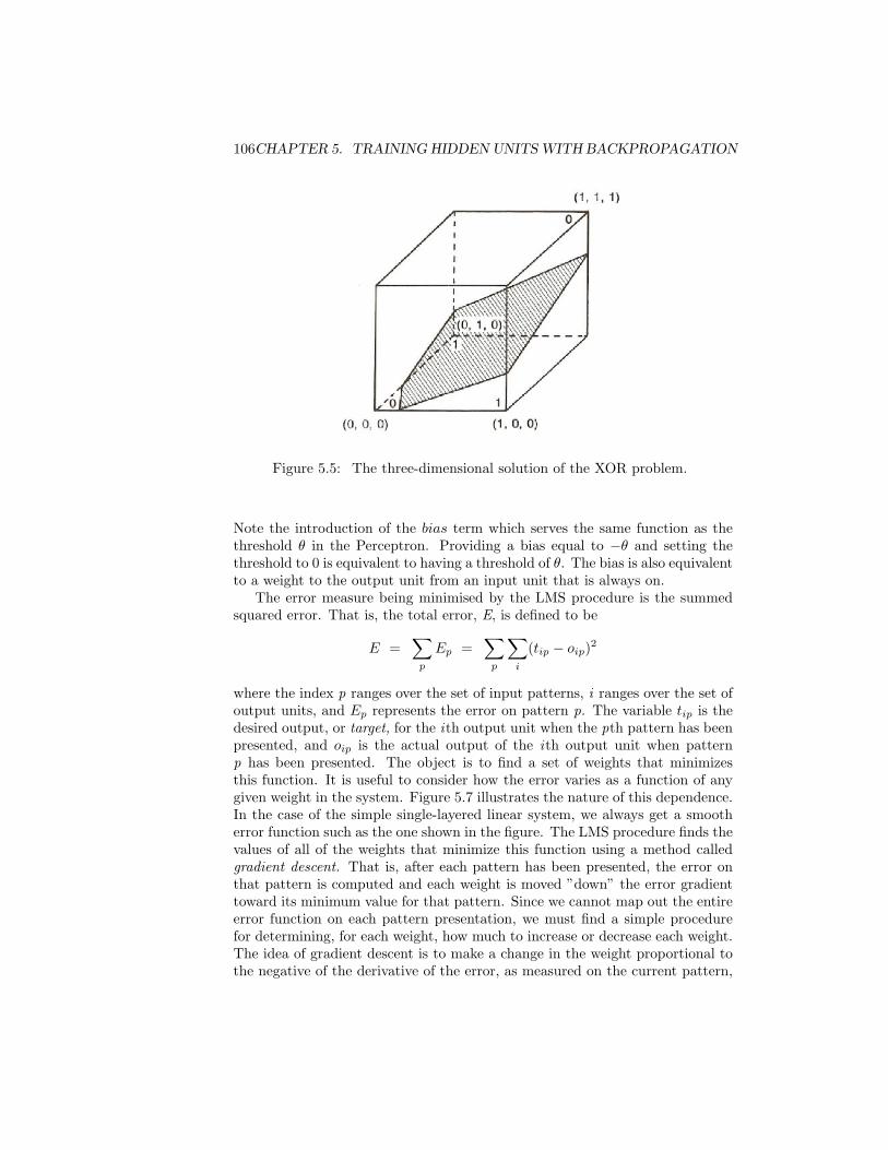
106CHAPTER 5. TRAINING HIDDEN UNITS WITH BACKPROPAGATION
Figure 5.5: The three-dimensional solution of the XOR problem.
Note the introduction of the bias term which serves the same function as thethreshold θ in the Perceptron. Providing a bias equal to −θ and setting thethreshold to 0 is equivalent to having a threshold of θ. The bias is also equivalentto a weight to the output unit from an input unit that is always on.
The error measure being minimised by the LMS procedure is the summedsquared error. That is, the total error, E, is defined to be
E =∑p
Ep =∑p
∑i
(tip − oip)2
where the index p ranges over the set of input patterns, i ranges over the set ofoutput units, and Ep represents the error on pattern p. The variable tip is thedesired output, or target, for the ith output unit when the pth pattern has beenpresented, and oip is the actual output of the ith output unit when patternp has been presented. The object is to find a set of weights that minimizesthis function. It is useful to consider how the error varies as a function of anygiven weight in the system. Figure 5.7 illustrates the nature of this dependence.In the case of the simple single-layered linear system, we always get a smootherror function such as the one shown in the figure. The LMS procedure finds thevalues of all of the weights that minimize this function using a method calledgradient descent. That is, after each pattern has been presented, the error onthat pattern is computed and each weight is moved ”down” the error gradienttoward its minimum value for that pattern. Since we cannot map out the entireerror function on each pattern presentation, we must find a simple procedurefor determining, for each weight, how much to increase or decrease each weight.The idea of gradient descent is to make a change in the weight proportional tothe negative of the derivative of the error, as measured on the current pattern,

5.1. BACKGROUND 107
Figure 5.6: A multilayer network that converts the two-dimensional three-dimensional XOR problem into a three-dimensional linearly separable problem.
with respect to each weight.1 Thus the learning rule becomes
∆wij = −k ∂Ep∂wij
where k is the constant of proportionality. Interestingly, carrying out the deriva-tive of the error measure in Equation 1 we get
∆wij = εδipiip
where ε = 2k and δip = (tip − oip) is the difference between the target for uniti on pattern p and the actual output produced by the network. This is exactlythe delta learning rule described in Equation 15 from Chapter 4. It shouldalso be noted that this rule is essentially the same as that for the perceptron.In the perceptron the learning rate was 1 (i.e., we made unit changes in theweights) and the units were binary, but the rule itself is the same: the weightsare changed proportionally to the difference between target and output timesthe input. If we change each weight according to this rule, each weight is movedtoward its own minimum and we think of the system as moving downhill inweight-space until it reaches its minimum error value. When all of the weightshave reached their minimum points, the system has reached equilibrium. If thesystem is able to solve the problem entirely, the system will reach zero error
1It should be clear from Figure 5.7 why we want the negation of the derivative. If the weightis above the minimum value, the slope at that point is positive and we want to decrease theweight; thus when the slope is positive we add a negative amount to the weight. On the otherhand, if the weight is too small, the error curve has a negative slope at that point, so we wantto add a positive amount to the weight.

108CHAPTER 5. TRAINING HIDDEN UNITS WITH BACKPROPAGATION
Figure 5.7: Typical curve showing the relationship between overall error andchanges in a single weight in the network.
and the weights will no longer be modified. If the network is unable to get theproblem exactly right, it will find a set of weights that produces as small anerror as possible.
In order to get a fuller understanding of this process it is useful to care-fully consider the entire error space rather than a one-dimensional slice. Ingeneral this is very difficult to do because of the difficulty of depicting and vi-sualizing high-dimensional spaces. However, we can usefully go from one to twodimensions by considering a network with exactly two weights. Consider, as anexample, a linear network with two input units and one output unit with thetask of finding a set of weights that comes as close as possible to performingthe function OR. Assume the network has just two weights and no bias termslike the network in Figure 5.1.1A. We can then give some idea of the shapeof the space by making a contour map of the error surface. Figure 5.8 showsthe contour map. In this case the space is shaped like a kind of oblong bowl.It is relatively flat on the bottom and rises sharply on the sides. Each equalerror contour is elliptically shaped. The arrows around the ellipses representthe derivatives of the two weights at those points and thus represent the di-rections and magnitudes of weight changes at each point on the error surface.The changes are relatively large where the sides of the bowl are relatively steepand become smaller and smaller as we move into the central minimum. Thelong, curved arrow represents a typical trajectory in weight-space from a start-ing point far from the minimum down to the actual minimum in the space. Theweights trace a curved trajectory following the arrows and crossing the contourlines at right angles.
The figure illustrates an important aspect of gradient descent learning. This

5.1. BACKGROUND 109
Figure 5.8: A contour map illustrating the error surface with respect to the twoweights w1 and w2 for the OR problem in a linear network with two weightsand no bias term. Note that the OR problem cannot be solved perfectly in alinear system. The minimum sum squared error over the four input-output pairsoccurs when w1 = w2 = 0.75. (The input-output pairs are 00− 0,01− 1,10− 1,and 11− 1.)
is the fact that gradient descent involves making larger changes to parametersthat will have the biggest effect on the measure being minimized. In this case,the LMS procedure makes changes to the weights proportional to the effectthey will have on the summed squared error. The resulting total change to theweights is a vector that points in the direction in which the error drops moststeeply.
5.1.2 The Backpropagation Rule
Although this simple linear pattern associator is a useful model for understand-ing the dynamics of gradient descent learning, it is not useful for solving prob-lems such as the XOR problem mentioned above. As pointed out in PDP:2,linear systems cannot compute more in multiple layers than they can in a singlelayer. The basic idea of the backpropagation method of learning is to combine anonlinear perceptron-like system capable of making decisions with the objective

110CHAPTER 5. TRAINING HIDDEN UNITS WITH BACKPROPAGATION
error function of LMS and gradient descent. To do this, we must be able toreadily compute the derivative of the error function with respect to any weightin the network and then change that weight according to the rule
∆wij = −k ∂Ep∂wij
How can this derivative be computed? First, it is necessary to use a differ-entiable output function, rather than the threshold function used in the per-ceptron convergence procedure. A common choice, and one that allows us torelate backpropagation learning to probabilistic inference, is to use the logisticfunction f(neti) = 1
1+exp(−neti) . Given a choice of f , we can then determinethe partial derivative of the Error with respect to a weight coming to an outputunit i from a unit j that projects to it.
We can use the chain rule to compute the partial derivative of the error withrespect to our particular weight wij :
∂Ep∂wij
=∂Ep∂aip
∂aip∂netip
∂netip∂wij
Now, Ep =∑i(tip − aip)2, so that ∂Ep
∂aipis equal to −2(tip − aip). ai =
f(neti),2 and, so that we can leave f unspecified for the moment, we writef ′(neti) to represent its derivative evaluated at neti. Finally, neti =
∑j ajwij ,
and its partial derivative of the net input with respect to wij is just aj . In sum,then we have
− ∂Ep∂wij
= 2(tip − aip)f ′(netip)ajp
Let us use δip to represent (tip−aip)f ′(netip). δip is proportional to (minus) thepartial derivative of the error with respect to the net input to unit i in patternp, ∂E
∂netip. Substituting this into the above expression, we can now write:
− ∂Ep∂wij
∝ δipajp
This generalizes the delta rule from the LMS procedure to the case where thereis a non-linearity applied to the output units, with the δ terms now defined soas to take this non-linearity into account.
Now let us consider a weight that projects from an input unit k to a hiddenunit j, which in turn projects to an output unit, i in a very simple networkconsisting of only one unit at each of these three layers (see Figure 5.1.2). Wecan ask, what is the partial derivative of the error on the output unit i withrespect to a change in the weight wjk to the hidden unit from the input unit? Itmay be helpful to talk yourself informally through the series of effects changing
2In the networks we will be considering in this chapter, the output of a unit is equal to itsactivation. We use the symbol a to designate this variable. This symbol can be used for anyunit, be it an input unit, an output unit, or a hidden unit.

5.1. BACKGROUND 111
Figure 5.9: A 1:1:1 network, consisting of one input unit, one hidden unit,and one output unit. In the text discussing the chain of effects of changing theweight from the input unit to the hidden unit on the error at the output unit,the index i is used for the output unit, j for the hidden unit j, and k for theinput unit.
such a weight would have on the error in this case. It should be obvious thatif you increase the weight to the hidden unit from the input unit, that willincrease the net input to the hidden unit j by an amount that depends on theactivation of the input unit k. If the input unit were inactive, the change inthe weight would have no effect; the stronger the activation of the input unit,the stronger the effect of changing the weight on the net input to the hiddenunit. This change, you should also see, will in turn increase the activation of thehidden unit; the amoung of the increase will depend on the slope (derivative)of the unit’s activation function evaluated at the current value of its net input.This change in the activation with then affect the net input to the output uniti by an amount depending on the current value of the weight to unit i fromunit j. This change in the net input to unit i will then affect the activationof unit i by an amount proportional to the derivative of its activation functionevaluated at the current value of its net input. This change in the activationof the output unit will then affect the error by an amount proportional to thedifference between the target and the current activation of the output unit.
The above is an intuitive account of corresponding to the series of factorsyou get when you apply the chain rule to unpack the partial derivative of theerror at the output unit with respect to a change in the weight to the hiddenunit from the input unit. Applying this to the case of the error on pattern p,

112CHAPTER 5. TRAINING HIDDEN UNITS WITH BACKPROPAGATION
we would write
∂Ep∂wjk
=∂Ep∂aip
∂aip∂neti
∂netip∂ajp
∂aip∂netj
∂netjp∂wjk
The factors in the chain are given in the reverse order from the verbal descriptionabove since this is how they will actually be calculated using backpropagation.The first two factors on the right correspond to the last two links of the chaindescribed above, and are equal to the δ term for output unit i as previouslydiscussed. The third factor is equal to the weight to output unit i from hiddenunit j; and the fourth factor corresponds to the derivative of the activationfunction of the hidden unit, evaluated at its net input given the current patternp, f ′(netjp). Taking these four factors together they correspond to (minus) thepartial derivative of the error at output unit i with respect to the net input tohidden unit j.
Now, if there is more than one output unit, the partial derivative of the erroracross all of the output units is just equal to the sum of the partial derivativesof the error with respect to each of the output units:
δjp = f ′(netjp)∑i
wijδip. BP Equation
The equation above is the core of the backpropagation process and we call itthe BP Equation for future reference.
Because ∂netjp∂wjk
equals akp, the partial derivative of the error with respect tothe weight then becomes:
− ∂Ep∂wjk
= δjpakp .
Although we have not demonstrated it here, it is easy to show that, withmore layers, the correct δ term for each unit j in a given layer of a feed-forwardnetwork is always equal to the derivative of the activation function of the unitevaluated at the current value of its net input, times the sum over the forwardconnections from that unit of the product of the weight on each forward con-nection times the delta term at the receiving end of that connection; i.e., the δterms for all layers are determined by applying the BP Equation.
Thus, once delta terms have been computed at the output layers of a feed-forward network, the BP equation can be used iteratively to calculate δ termsbackward across many layers of weights, and to specify how each weight shouldbe changed to perform gradient decent. Thus we now have a generalized versionof the delta rule that specifies a procedure for changing all the weights in alllaters of a feed forward network: If we adjust the weight to each output unit ifrom each unit j projecting to it, by an amount proportional to δipajp, where δjis defined recursively as discussed above, we will be performing gradient descentin E: We will be adjusting each weight in proportion to (minus) the effect thatits adjustment would have on the error.

5.1. BACKGROUND 113
The application of the backpropagation rule, then, involves two phases: Dur-ing the first phase the input is presented and propagated forward through thenetwork to compute the output value aip for each unit. This output is thencompared with the target, and scaled by the derivative of the activation func-tion, resulting in a δ term for each output unit. The second phase involvesa backward pass through the network (analogous to the initial forward pass)during which the δ term is computed for each unit in the network. This second,backward pass allows the recursive computation of δ as indicated above. Oncethese two phases are complete, we can compute, for each weight, the product ofthe δ term associated with the unit it projects to times the activation of the unitit projects from. Henceforth we will call this product the weight error derivativesince it is proportional to (minus) the derivative of the error with respect to theweight. As will be discussed later, these weight error derivatives can then beused to compute actual weight changes on a pattern-by-pattern basis, or theymay be accumulated over the ensemble of patterns with the accumulated sumof its weight error derivatives then being applied to each of the weights.
Adjusting bias weights. Of course, the generalized delta rule can also beused to learn biases, which we treat as weights from a special “bias unit” that isalways on. A bias weight can project from this unit to any unit in the network,and can be adjusted like any other weight, with the further stipulation that theactivation of the sending unit in this case is always fixed at 1.
The activation function. As stated above, the derivation of the backpropaga-tion learning rule requires that the derivative of the activation function, f ′(neti)exists. It is interesting to note that the linear threshold function, on which theperceptron is based, is discontinuous and hence will not suffice for backpropa-gation. Similarly, since a network with linear units achieves no advantage fromhidden units, a linear activation function will not suffice either. Thus, we needa continuous, nonlinear activation function. In most of our work on backprop-agation and in the program presented in this chapter, we have used the logisticactivation function.
In order to apply our learning rule, we need to know the derivative of thisfunction with respect to its net input. It is easy to show that this derivative isequal to aip(1 − aip). This expression can simply be substituted for f ′(net) inthe derivations above.
It should be noted that aip(1 − aip) reaches its maximum when aip = 0.5and goes to 0 as aip approaches 0 or 1 (see Figure 5.1.2). Since the amountof change in a given weight is proportional to this derivative, weights will bechanged most for those units that are near their midrange and, in some sense,not yet committed to being either on or off. This feature can sometimes leadto problems for backpropagation learning, and the problem can be especiallyserious at the output layer. If the weights in a network at some point duringlearning are such that a unit that should be on is completely off (or a unit thatshould be off is completely on) the error at that unit is large but paradoxicallythe delta term at that unit is very small, and so no error signal is propagatedback through the network to correct the problem.
An improved error measure. There are various ways around the problem

114CHAPTER 5. TRAINING HIDDEN UNITS WITH BACKPROPAGATION
Figure 5.10: The logistic function and its derivative.
just noted above. One is to simply leave the f ′(neti) term out of the calculationof delta terms at the output units. In practice, this solves the problem, but itseems like a bit of a hack.
Interestingly, however, if the error measure E is replaced by a different mea-sure, called the ’cross-entropy’ error, here called CE, we obtain an elegant result.The cross-entropy error for pattern p is defined as
CEp = −∑i
[tip log(aip) + (1− tip) log(1− aip)]
If the target value tip is thought of as a binary random variable having valueone with probability pip, and the activation of the output unit aip is construedas representing the network’s estimate of that probability, the cross-entropymeasure corresponds to the negative logarithm of the probability of the observedtarget values, given the current estimates of the pip’s. Minimizing the cross-entropy error corresponds to maximizing the probability of the observed targetvalues. The maximum is reached when for all i and p, aip = pip.
Now very neatly, it turns out that the derivative of CEp with respect to aipis
−[tipaip
+1− tip)
(1− aip)
].
When this is multiplied times the derivative of the logistic function evaluatedat the net input, aip(1 − aip), to obtain the corresponding δ term δip, severalthings cancel out and we are left with
δip = tip − aip.
This is the same expression for the δ term we would get using the standardsum squared error measure E, if we simply ignored the derivative of the activa-tion function! Because using cross entropy error seems more appropriate thansummed squared error in many cases and also because it often works better, we

5.1. BACKGROUND 115
provide the option of using the cross entropy error in the pdptool backpropa-gation simulator.
Even using cross-entropy instead of sum squared error, it sometimes happensthat hidden units have strong learned input weights that ’pin’ their activationagainst 1 or 0, and in that case it becomes effectively impossible to propagateerror back through these units. Different solutions to this problem have beenproposed. One is to use a small amount of weight decay to prevent weights fromgrowing too large. Another is to add a small constant to the derivative of theactivation function of the hidden unit. This latter method works well, but isoften considered a hack, and so is not implemented in the pdptool software.Weight decay is available in the software, however, and is described below.
Local minima. Like the simpler LMS learning paradigm, backpropagation isa gradient descent procedure. Essentially, the system will follow the contour ofthe error surface, always moving downhill in the direction of steepest descent.This is no particular problem for the single-layer linear model. These systemsalways have bowl-shaped error surfaces. However, in multilayer networks thereis the possibility of rather more complex surfaces with many minima. Some ofthe minima constitute complete solutions to the error minimization problem, inthe sense at these minima the system has reached a completely errorless state.All such minima are global minima. However, it is possible for there to be someresidual errror at the bottom of some of the minima. In this case, a gradientdescent method may not find the best possible solution to the problem at hand.
Part of the study of backpropagation networks and learning involves a studyof how frequently and under what conditions local minima occur. In networkswith many hidden units, local minima seem quite rare. However with few hiddenunits, local minima can occur. The simple 1:1:1 network shown in Figure 5.1.2can be used to demonstate this phenomenon. The problem posed to this networkis to copy the value of the input unit to the output unit. There are two basicways in which the network can solve the problem. It can have positive biases onthe hidden unit and on the output unit and large negative connections from theinput unit to the hidden unit and from the hidden unit to the output unit, or itcan have large negative biases on the two units and large positive weights fromthe input unit to the hidden unit and from the hidden unit to the output unit.These solutions are illustrated in Figure 5.11. In the first case, the solutionworks as follows: Imagine first that the input unit takes on a value of 0. In thiscase, there will be no activation from the input unit to the hidden unit, butthe bias on the hidden unit will turn it on. Then the hidden unit has a strongnegative connection to the output unit so it will be turned off, as required inthis case. Now suppose that the input unit is set to 1. In this case, the stronginhibitory connection from the input to the hidden unit will turn the hiddenunit off. Thus, no activation will flow from the hidden unit to the output unit.In this case, the positive bias on the output unit will turn it on and the problemwill be solved. Now consider the second class of solutions. For this case, theconnections among units are positive and the biases are negative. When theinput unit is off, it cannot turn on the hidden unit. Since the hidden unit hasa negative bias, it too will be off. The output unit, then, will not receive any

116CHAPTER 5. TRAINING HIDDEN UNITS WITH BACKPROPAGATION
Figure 5.11:
input from the hidden unit and since its bias is negative, it too will turn offas required for zero input. Finally, if the input unit is turned on, the strongpositive connection from the input unit to the hidden unit will turn on thehidden unit. This in turn will turn on the output unit as required. Thus wehave, it appears, two symmetric solutions to the problem. Depending on therandom starting state, the system will end up in one or the other of these globalminima.
Interestingly, it is a simple matter to convert this problem to one with onelocal and one global minimum simply by setting the biases to 0 and not allowingthem to change. In this case, the minima correspond to roughly the same twosolutions as before. In one case, which is the global minimum as it turns out,both connections are large and negative. These minima are also illustrated inFigure 5.11. Consider first what happens with both weights negative. When theinput unit is turned off, the hidden unit receives no input. Since the bias is 0,the hidden unit has a net input of 0. A net input of 0 causes the hidden unit totake on a value of 0.5. The 0.5 input from the hidden unit, coupled with a largenegative connection from the hidden unit to the output unit, is sufficient toturn off the output unit as required. On the other hand, when the input unit isturned on, it turns off the hidden unit. When the hidden unit is off, the outputunit receives a net input of 0 and takes on a value of 0.5 rather than the desiredvalue of 1.0. Thus there is an error of 0.5 and a squared error of 0.25. This, itturns out, is the best the system can do with zero biases. Now consider whathappens if both connections are positive. When the input unit is off, the hiddenunit takes on a value of 0.5. Since the output is intended to be 0 in this case,there is pressure for the weight from the hidden unit to the output unit to besmall. On the other hand, when the input unit is on, it turns on the hidden unit.

5.1. BACKGROUND 117
Since the output unit is to be on in this case, there is pressure for the weight tobe large so it can turn on the output unit. In fact, these two pressures balanceoff and the system finds a compromise value of about 0.73. This compromiseyields a summed squared error of about 0.45—a local minimum.
Usually, it is difficult to see why a network has been caught in a local min-imum. However, in this very simple case, we have only two weights and canproduce a contour map for the error space. The map is shown in Figure 5.1.2.It is perhaps difficult to visualize, but the map roughly shows a saddle shape.It is high on the upper left and lower right and slopes down toward the center.It then slopes off on each side toward the two minima. If the initial values ofthe weights begin one part of the space, the system will follow the contoursdown and to the left into the minimum in which both weights are negative. If,however, the system begins in another part of the space, the system will fol-low the slope into the upper right quadrant in which both weights are positive.Eventually, the system moves into a gently sloping valley in which the weightfrom the hidden unit to the output unit is almost constant at about 0.73 andthe weight from the input unit to the hidden unit is slowly increasing. It isslowly being sucked into a local minimum. The directed arrows superimposedon the map illustrate thelines of force and illustrate these dynamics. The longarrows represent two trajectories through weightspace for two different startingpoints.
It is rare that we can create such a simple illustration of the dynamics ofweight-spaces and see how clearly local minima come about. However, it is likelythat many of our spaces contain these kinds of saddle-shaped error surfaces.Sometimes, as when the biases are free to move, there is a global minimum oneither side of the saddle point. In this case, it doesn’t matter which way youmove off. At other times, such as in Figure 5.1.2, the two sides are of differentdepths. There is no way the system can sense the depth of a minimum from theedge, and once it has slipped in there is no way out. Importantly, however, wefind that high-dimensional spaces (with many weights) have relatively few localminima.
Momentum. Our learning procedure requires only that the change in weightbe proportional to the weight error derivative. True gradient descent requiresthat infinitesimal steps be taken. The constant of proportionality, ε, is thelearning rate in our procedure. The larger this constant, the larger the changesin the weights. The problem with this is that it can lead to steps that overshootthe minimum, resulting in a large increase in error. For practical purposes wechoose a learning rate that is as large as possible without leading to oscillation.This offers the most rapid learning. One way to increase the learning ratewithout leading to oscillation is to modify the backpropagation learning rule toinclude a momentum term. This can be accomplished by the following rule:
∆wij(n+ 1) = ε(δipajp) + α∆wij(n)
where the subscript n indexes the presentation number and α is a constant thatdetermines the effect of past weight changes on the current direction of move-ment in weight space. This provides a kind of momentum in weight-space that

118CHAPTER 5. TRAINING HIDDEN UNITS WITH BACKPROPAGATION
Figure 5.12: A contour map for the 1:1:1 identity problem with biases fixedat 0. The map show a local minimum in the positive quadrant and a globalminimum in the lower left-hand negative quadrant. Overall the error surface issaddle-shaped. See the text for further explanation.
effectively filters out high-frequency variations of the error surface in the weight-space. This is useful in spaces containing long ravines that are characterized bysteep walls on both sides of the ravine and a gently sloping floor. Such situationstend to lead to divergent oscillations across the ravine. To prevent these it isnecessary to take very small steps, but this causes very slow progress along theravine. The momentum tends to cancel out the tendency to jump across theravine and thus allows the effective weight steps to be bigger. In most of thesimulations reported in PDP:8, α was about 0.9. Our experience has been thatwe get the same solutions by setting α = 0 and reducing the size of ε, but thesystem learns much faster overall with larger values of α and ε.
Symmetry breaking. Our learning procedure has one more problem that canbe readily overcome and this is the problem of symmetry breaking. If all weightsstart out with equal values and if the solution requires that unequal weights bedeveloped, the system can never learn. This is because error is propagated backthrough the weights in proportion to the values of the weights. This means thatall hidden units connected directly to the output units will get identical error

5.1. BACKGROUND 119
signals, and, since the weight changes depend on the error signals, the weightsfrom those units to the output units must always be the same. The systemis starting out at a kind of unstable equilibrium point that keeps the weightsequal, but it is higher than some neighboring points on the error surface, andonce it moves away to one of these points, it will never return. We counteractthis problem by starting the system with small random weights. Under theseconditions symmetry problems of this kind do not arise. This can be seen inFigure 5.1.2. If the system starts at exactly (0,0), there is no pressure for it tomove at all and the system will not learn; if it starts virtually anywhere else, itwill eventually end up in one minimum or the other.
Weight decay. One additional extension of the backpropagation model thatwe will consider here is the inclusion of weight decay. Weight decay is simply atendency for weights to be reduced very slightly every time they are updated.If weight-decay is non-zero, then the full equation for the change to each weightbecomes the following:
∆wij(n+ 1) = ε(δipajp)− ωwij(n) + α∆wij(n)
where ω is a positive constant representing the strength of the weight decay.Weight decay can be seen as a procedure for minimizing the total magnitude ofthe weights, where the magnitude is the sum of the squares of the weights. Itshould be noted that minimizing the sum of the squares of the weights can bein competition with minimizing the error measure, and so if weight decay is toostrong it can often interfere with reaching an acceptable performance criterion.
Learning by pattern or by epoch. The derivation of the backpropagation rulepresupposes that we are taking the derivative of the error function summedover all patterns. In this case, we might imagine that we would present allpatterns and then sum the derivatives before changing the weights. Instead,we can compute the derivatives on each pattern and make the changes to theweights after each pattern rather than after each epoch. Although the formerapproach can be implemented more efficiently (weight error derivatives for eachpattern can be computed in parallel over separate processors, for example) thelatter approach may be more plausible from a human or biological learningperspective, where it seems that learning does occur “on line”. Also, if thetraining set is large, consistent weight error derivatives across patterns can addup and produce a huge overshoot in the change to a connection weight. Thebp program allows weight changes after each pattern or after each epoch. Infact, the user may specify the size of a batch of patterns to be processed beforeweights are updated.3
3We moving between these options, it is important to note that weight decay is appliedeach time weights are updated. If weights are updated after each pattern, a smaller value ofweight decay should be used than if they are updated after a batch of n patterns or a wholeepoch.

120CHAPTER 5. TRAINING HIDDEN UNITS WITH BACKPROPAGATION
5.2 IMPLEMENTATION
The bp program implements the backpropagation process just described. Net-works are assumed to be feedforward only, with no recurrence. An implementa-tion of backpropagation for recurrent networks is described in a later chapter.
The network is specified in terms of a set of pools of units. By convention,pools(1) contains the single bias unit, which is always on. Subsequent poolsare declared in an order that corresponds to the feed-forward structure of thenetwork. Since activations at later layers depend on the activations at earlierlayers, the activations of units must be processed in correct order, and thereforethe order of specification of pools of units is important. Indeed, since deltasat each layer depend on the delta terms from the layers further forward, thebackward pass must also be carried out in the correct order. Each pool has atype: it can be an input pool, an output pool, or a hidden pool. There can bemore than one input pool and more than one output pool and there can be 0or more hidden pools. Input pools must all be specified before any other poolsand all hidden pools must be specified before any output pools.
Connections among units are specified by projections. Projections may befrom any pool to any higher numbered pool; since the bias pool is pools(1) itmay project to any other pool, although bias projections to input pools willhave no effect since activations of input units are clamped to the value specifiedby the external input. Projections from a layer to itself are not allowed.
Weights in a projection can be constrained to be positive or negative. Theseconstraints are imposed both at initialization and after each time the weights areincremented during processing. Two other constraints are imposed only whenweights are initialized; these constraints specify either a fixed value to which theweight is initialized, or a random value. For weights that are random, if theyare constrained to be positive, they are initialized to a value between 0 and thevalue of a parameter called wrange; if the weights are constrained to be negative,the initialization value is between -wrange and 0; otherwise, the initializationvalue is between wrange/2 and -wrange/2. Weights that are constrained to afixed value are initialized to that value.
The program also allows the user to set an individual learning rate for eachprojection via a layer-specific lrate parameter. If the value of this layer-specificlrate is unspecified, the network-wide lrate variable is used.
The bp program also makes use of an environment comprising a list ofpattern pairs, each pair consisting of a name, an input pattern, and a targetpattern. The number of elements in the input pattern should be equal to thetotal number of units summed across all input pools. Similarly, the number ofelements of the target pattern should be equal to the total number of outputunits summed across all output pools.
Processing of a single pattern occurs as follows: A pattern pair is chosen,and the pattern of activation specified by the input pattern is clamped on theinput units; that is, their activations are set to whatever numerical values arespecified in the input pattern. These are typically 0’s and 1’s but may take anyreal value.

5.2. IMPLEMENTATION 121
Next, activations are computed. For each non-input pool, the net inputsto each unit are computed and then the activations of the units are set. Thisoccurs in the order that the pools are specified in the network specification,which must be specified correctly so that by the time each unit is encountered,the activations of all of the units that feed into it have already been set. Theroutine performing this computation is called compute output. Once the outputhas been computed some summary statistics are computed in a routine calledsumstats. First it computes the pattern sum of squares (pss), equal to thesquared error terms summed over all of the output units. Analogously, the pceor pattern cross entropy, the sum of the cross entropy terms accross all theoutput units, is calculated. Then the routine adds the pss to the total sum ofsquares (tss), which is just the cumulative sum of the pss for all patterns thusfar processed within the current epoch. Similarly the pce is added to the tce, ortotal cross entropy measure.
Next, error and delta terms are computed in a routine called compute error.The error for a unit is equivalent to (minus) the partial derivative of the errorwith respect to a change in the activation of the unit. The delta for the unit is(minus) the partial derivative of the error with respect to a change in the netinput to the unit. First, the error terms are calculated for each output unit.For these units, error is the difference between the target and the obtainedactivation of the unit. After the error has been computed for each output unit,we get to the ”heart” of backpropagation: the recursive computation of errorand delta terms for hidden units. The program iterates backward over the layers,starting with the last output layer. The first thing it does in each layer is set thevalue of delta for the units in the current layer; this is equal to the error for theunit times the derivative of the activation function as described above. Then,once it has the delta terms for the current pool, the program passes this backto all pools that project to the current pool; this is the actual backpropagationprocess. By the time a particular pool becomes the current pool, all of the unitsthat it projects to will have already been processed and its total error will havebeen accumulated, so it is ready to have its delta computed.
After the backward pass, the weight error derivatives are then computedfrom the deltas and activations in a routine called compute weds. Note thatthis routine adds the weight error derivatives occasioned by the present patterninto an array where they can potentially be accumulated over patterns.
Weight error derivatives actually lead to changes in the weights when aroutine called change weights is called. This may be called after each patternhas been processed, or after each batch of n patterns, or after all patterns inthe training set have been processed. When this routine is called, it cyclesthrough all the projections in the network. For each, the new delta weight isfirst calculated. The delta weight is equal to (1) the accumulated weight errorderivative scaled by the lrate, minus the weight decay scaled by wdecay, plusa fraction of the previous delta weight where the fraction is the value of themomentum parameter. Then, this delta weight is added into the weight, sothat the weight’s new value is equal to its old value plus the delta weight. Atthe end of processing each projection, the weight error derivative terms are all

122CHAPTER 5. TRAINING HIDDEN UNITS WITH BACKPROPAGATION
set to 0, and constraints on the values of the weights are reset.Generally, learning is accomplished through a sequence of epochs, in which
all pattern pairs are presented for one trial each during each epoch. The pre-sentation is either in sequential or permuted order. It is also possible to test theprocessing of patterns, either individually or by sequentially cycling through thewhole list, with learning turned off. In this case, compute output, compute error,and sumstats are called, but compute wed and change weights are not called.
5.3 RUNNING THE PROGRAM
The bp program is used much like earlier programs in this series, particularlypa. Like the other programs, it has a flexible architecture that is specified usinga .m file, and a flexible screen layout that is specified in a .tem file. The programalso makes use of a .pat file, in which the pairs of patterns to be used in trainingand testing the network are listed.
When networks are initialized, the weights are generally assigned accordingto a pseudo-random number generator. As in pa and iac, the reset commandallows the user to repeat a simulation run with the same initial configurationused just before. (Another procedure for repeating the previous run is describedin Ex. 5.1.) The newstart command generates a new random seed and seedsthe random number generator with it before using the seed in generating a newset of random initial values for the connection weights.
Control over learning occurs by setting options in the training window orvia the settrainopts function. The number of epochs nepochs to train each time“run” is called can be specified. The user can also specify whether weights areupdated after every pattern, after n patterns, or after every epoch, and whetherthe mode of pattern presentation is sequential s or permuted p. The learningrate, weight decay, and momentum parameters can all be specified as well. Theuser can also set a stopping criterion for training called “ecrit”. The variablewrange, the range of values allowed when weights are initialized or re-initialized,can also be adjusted.
fast mode for training. The bp program’s inner loops have been converted tofast mex code (c code that interfaces with MATLAB). To turn on the fast modefor network training, click the ’fast’ option in the train window. This optioncan also be set by typing the following command on the MATLAB commandprompt:runprocess(’process’,’train’,’granularity’,’epoch’,’count’,1,’fastrun’,1);
There are some limitations in executing fast mode of training.In this mode,network output logs can only be written at epoch level. Any smaller outputfrequency if specified, will be ignored.When running with fast code in gui mode,network viewer will only be updated at epoch level.Smaller granularity of displayupdate is disabled to speed up processing. The ’cascade’ option of buildingactivation gradually is also not available in fast mode.
There is a known issue with running this on linux OS.MATLAB processesrunning fast version appear to be consuming a lot of system memory. This

5.4. EXERCISES 123
memory management issue has not been observed on windows. We are currentlyinvestigating this and will be updating the documentation as soon as we find afix.
In the bp program the principle measures of performance are the patternsum of squares (pss) and the total sum of squares (tss), and the pattern cross-entropy pce and the total cross entropy tce. The user can specify whether theerror measure used in computing error derivatives is the sum squared error orthe cross entropy. Because of its historical precedence, the sum squared error isused by default. The user may optionally also compute an additional measure,the vector correlation of the present weight error derivatives with the previousweight error derivatives. The set of weight error derivatives can be thought ofas a vector pointing in the steepest direction downhill in weight space; thatis, it points down the error gradient. Thus, the vector correlation of thesederivatives across successive epochs indicates whether the gradient is stayingrelatively stable or shifting from epoch to epoch. For example, a negative valueof this correlation measure (called gcor for gradient correlation) indicates thatthe gradient is changing in direction. Since the gcor can be thought of asfollowing changes in the direction of the gradient, the check box for turning onthis computation is called follow
Control over testing is straightforward. With the “test all” box checked, theuser may either click run to carry out a complete pass through the test set, orclick step to step pattern by pattern, or the user may uncheck the “text all”button and select an individual pattern by clicking on it in the network viewerwindow and then clicking run or step.
There is a special mode available in the bp program called cascade mode.This mode allows activation to build up gradually rather than being computedin a single step as is usually the case in bp. A discussion of the implementationand use of this mode is provided later in this chapter.
As with other pdptool programs the user may adjust the frequency of dis-play updating in the train and test windows. It is also possible to log and creategraphs of the state of the network at the pattern or epoch level using create/editlogs within the training and testing options panels.
5.4 EXERCISES
We present four exercises using the basic backpropagation procedure. The firstone takes you through the XOR problem and is intended to allow you to testand consolidate your basic understanding of the backpropagation procedureand the gradient descent process it implements. The second allows you toexplore the wide range of different ways in which the XOR problem can besolved; as you will see the solution found varies from run to run initialized withdifferent starting weights. The third exercise suggests minor variations of thebasic backpropagation procedure, such as whether weights are changed patternby pattern or epoch by epoch, and also proposes various parameters that may beexplored. The fourth exercise suggests other possible problems that you might

124CHAPTER 5. TRAINING HIDDEN UNITS WITH BACKPROPAGATION
Figure 5.13: Architecture of the XOR network used in the exercises (FromPDP:8, p.332.)
want to explore using backpropagation.
Ex5.1. The XOR Problem
The XOR problem is described at length in PDP:8. Here we will be consideringone of the two network architectures considered there for solving this problem.This architecture is shown in Figure 5.13. In this network configuration thereare two input units, one for each “bit” in the input pattern. There are also twohidden units and one output unit. The input units project to the hidden units,and the hidden units project to the output unit; there are no direct connectionsfrom the input units to the output units.
All of the relevant files for doing this exercise are contained in the bp direc-tory; they are called bp xor.tem, bp xor.m, bp xor.pat, and xor.wt.
Once you have downloaded the latest version of the software, started MAT-LAB, set your path to include the pdptool directory and all of its children, andchanged to the bp directory, you can simply type
bpxorto the MATLAB command-line prompt. This file instructs the program to setup the network as specified in the bp xor.m file and to read the patterns asspecified in the bp xor.pat file; it also initializes various variables. Then it readsin an initial set of weights to use for this exercise. Finally, a test of all of thepatterns in the training set is performed. The network viewer window thatfinally appears shows the state of the network at the end of this initial test ofall of the patterns. It is shown in Figure 5.14.
The display area in the network viewer window shows the current epoch

5.4. EXERCISES 125
Figure 5.14: The display produced by the bp program, initialized for XOR.
number and the total sum of of squares (tss) resulting from testing all fourpatterns. The next line contains the value of the gcor variable, currently 0 sinceno error derivatives have yet been calculated. Below that is a line containingthe current pattern name and the pattern sum of squares pss associated withthis pattern. To the right in the “patterns” panel is the set of input and targetpatterns for XOR. Back in the main network viewer window, we now turn ourattention to the area to the right and below the label “sender acts”. The coloredsquares in this row shows the activations of units that send their activationsforward to other units in the network. The first two are the two input units,and the next two are the two hidden units. Below each set of sender activationsare the corresponding projections, first from the input to the hidden units,and below and to the right of that, from the hidden units to the single outputunit. The weight in a particular column and row represents the strength of theconnection from a particular sender unit indexed by the column to the particularreceiver indexed by the row.
To the right of the weights is a column vector indicating the values of thebias terms for the receiver units-that is, all the units that receive input fromother units. In this case, the receivers are the two hidden units and the outputunit.
To the right of the biases is a column for the net input to each receiving unit.There is also a column for the activations of each of these receiver units. (Notethat the hidden units’ activations appear twice, once in the row of senders andonce in this column of receivers.) The next column contains the target vector,which in this case has only one element since there is only one output unit.Finally, the last column contains the delta values for the hidden and output

126CHAPTER 5. TRAINING HIDDEN UNITS WITH BACKPROPAGATION
units.Note that shades of red are used to represent positive values, shades of blue
are used for negative values, and a neutral gray color is used to represent 0.The color scale for weights, biases, and net inputs ranges over a very broadrange, and values less than about .5 are very faint in color. The color scalefor activations ranges over somewhat less of a range, since activations can onlyrange from 0 to 1. The color scale for deltas ranges over a very small rangesince delta values are very small. Even so, the delta values at the hidden levelshow very faintly compared with those at the output level, indicating just howsmall these delta values tend to be, at least at this early stage of training. Youcan inspect the actual numberical values of each variable by moving your mouseover the corresponding colored square.
The display shows what happened when the last pattern pair in the filebp xor.pat was processed. This pattern pair consists of the input pattern (1 1)and the target pattern (0). This input pattern was clamped on the two inputunits. This is why they both have activation values of 1.0, shown as a fairlysaturated red in the first two entries of the sender activation vector. With theseactivations of the input units, coupled with the weights from these units to thehidden units, and with the values of the bias terms, the net inputs to the hiddenunits were set to 0.60 and -0.40, as indicated in the net column. Plugging thesevalues into the logistic function, the activation values of 0.64 and 0.40 wereobtained for these units. These values are shown both in the sender activationvector and in the receiver activation vector (labeled act, next to the net inputvector). Given these activations for the hidden units, coupled with the weightsfrom the hidden units to the output unit and the bias on the output unit, thenet input to the output unit is 0.48, as indicated at the bottom of the netcolumn. This leads to an activation of 0.61, as shown in the last entry of theact column. Since the target is 0.0, as indicated in the target column, the error,or (target - activation) is -0.61; this error, times the derivative of the activationfunction (that is, activation (1 - activation)) results in a delta value of -0.146,as indicated in the last entry of the final column. The delta values of the hiddenunits are determined by back propagating this delta term to the hidden units,using the backpropagation equation.
Q.5.1.1.
Show the calculations of the values of delta for each of the two hiddenunits, using the activations and weights as given in this initial screendisplay, and the BP Equation. Explain why these values are so small.
At this point, you will notice that the total sum of squares before any learninghas occurred is 1.0507. Run another tall to understand more about what ishappening.
Q.5.1.2.
Report the output the network produces for each input pattern andexplain why the values are all so similar, referring to the strengths of

5.4. EXERCISES 127
the weights, the logistic function, and the effects of passing activationforward through the hidden units before it reaches the output units.
Now you are ready to begin learning. Activate the training panel. If youclick run (don’t do that yet), this will run 30 epochs of training, presenting eachpattern sequentially in the order shown in the patterns window within eachepoch, and adjusting the weights at the end of the epoch. If you click step, youcan follow the tss and gcor measures as they change from epoch to epoch. Agraph will also appear showing the tss. If you click run after clicking step a fewtimes, the network will run to the 30 epoch milestone, then stop.
You may find in the course of running this exercise that you need to go backand start again. To do this, you should use the reset command, followed byclicking on the load weights button, and selecting the file bp xor.wt. This filecontains the initial weights used for this exercise. This method of reinitializingguarantees that all users will get the same starting weights.
After completing the first 30 epochs, stop and answer this question.
Q.5.1.3.
The total sum of squares is smaller at the end of 30 epochs, but isonly a little smaller. Describe what has happened to the weightsand biases and the resulting effects on the activation of the outputunits. Note the small sizes of the deltas for the hidden units andexplain. Do you expect learning to proceed quickly or slowly fromthis point? Why?
Run another 90 epochs of training (for a total of 120) and see if your pre-dictions are confirmed. As you go along, watch the progression of the tss in thegraph that should be displayed (or keep track of this value at each 30 epochmilestone by recording it manually). You might find it interesting to observethe results of processing each pattern rather than just the last pattern in thefour-pattern set. To do this, you can set the update after selection to 1 pat-tern rather than 1 epoch, and use the step button for an epoch or two at thebeginning of each set of 30 epochs.
At the end of another 60 epochs (total: 180), some of the weights in thenetwork have begun to build up. At this point, one of the hidden units isproviding a fairly sensitive index of the number of input units that are on. Theother is very unresponsive.
Q.5.1.4.
Explain why the more responsive hidden unit will continue to changeits incoming weights more rapidly than the other unit over the nextfew epochs.
Run another 30 epochs. At this point, after a total of 210 epochs, one of thehidden units is now acting rather like an OR unit: its output is about the samefor all input patterns in which one or more input units is on.

128CHAPTER 5. TRAINING HIDDEN UNITS WITH BACKPROPAGATION
Q.5.1.5.
Explain this OR unit in terms of its incoming weights and bias term.What is the other unit doing at this point?
Now run another 30 epochs. During these epochs, you will see that thesecond hidden unit becomes more differentiated in its response.
Q.5.1.6.
Describe what the second hidden unit is doing at this point, andexplain why it is leading the network to activate the output unitmost strongly when only one of the two input units is on.
Run another 30 epochs. Here you will see the tss drop very quickly.
Q.5.1.7.
Explain the rapid drop in the tss, referring to the forces operatingon the second hidden unit and the change in its behavior. Note thatthe size of the delta for this hidden unit at the end of 270 epochs isabout as large in absolute magnitude as the size of the delta for theoutput unit. Explain.
Click the run button one more time. Before the end of the 30 epochs, thevalue of tss drops below ecrit, and so training stops. The XOR problem is solvedat this point.
Q.5.1.8.
Summarize the course of learning, and compare the final state ofthe weights with their initial state. Can you give an approximateintuitive account of what has happened? What suggestions mightyou make for improving performance based on this analysis?
Ex5.2. Learning XOR with different initial weights
Run the XOR problem several more times, each time using newstart to get anew random configuration of weights. Write down the value of the random seedafter each newstart (you will find it by clicking on Set Seed in the upper lefthand corner of the network viewer window). Then run for up to 1000 epochs,or until the tss reaches the criterion (you can set nepochs in the test window to1000, and set update after to, say, 50 epochs). We will call cases in which thetss reaches the criterion successful cases. Continue until you find two successfulruns that reach different solutions than the one found in Exercise 5.1. Read onfor further details before proceeding.
Q.5.2.1.

5.4. EXERCISES 129
At the end of each run, record, after each random seed, the finalepoch number, and the final tss. Create a table of these results toturn in as part of your homework. Then, run through a test, inspect-ing the activations of each hidden unit and the single output unitobtained for each of the four patterns. Choose two successful runsthat seem to have reached different solutions than the one reachedin Exercise 5.1, as evidenced by qualitative differences in the hiddenunit activation patterns. For these two runs, record the hidden andoutput unit activations for each of the four patterns, and includethese results in a second table as part of what you turn in. For eachcase, state what logical predicate each hidden unit appears to be cal-culating, and how these predicates are then combined to determinethe activation of the output unit. State this in words for each case,and also use the notation described in the hint below to express thisinformation succinctly.
Hint. The question above may seem hard at first, but should become easieras you consider each case. In Excercise 5.1, one hidden unit comes on wheneither input unit is on (i.e., it acts as an OR unit), and the other comes onwhen both input units are on (i.e., it acts as an AND unit). For this exercise,we are looking for qualitatively different solutions. You might find that onehidden unit comes on when the first input unit is on and the second is off (Thiscould be called ‘A and not B’), and the other comes on when the first is on andthe second is off (‘B and not A’). The weights from the hidden units to the outputunit will be different from what they were in Exercise 5.1, reflecting a differencein the way the predicates computed by each hidden unit are combined to solvethe XOR problem. In each case you should be able to describe the way theproblem is being solved using logical expressions. Use A for input unit 1, B forinput unit 2, and express the whole operation as a compound logical statement,using the additional logical terms ’AND’ ’OR’ and ’NOT’. Use square bracketsaround the expression computed by each hidden unit, then use logical terms toexpress how the predicates computed by each hidden unit are combined. Forexample, for the case in Exercise 5.1, we would write: [A OR B] AND NOT [AAND B].
Ex5.3. Effects of parameters on XOR Learning.
There are several further studies one can do with XOR. You can study theeffects of varying:
1. One of the parameters of the model (lrate, wrange, momentum).2. Frequency of weight updating: once per pattern or epoch.3. The training regime: permuted vs. sequential presentation. This makes
a difference only when the frequency of weight updating is equal to pattern.4. The magnitude of the initial random weights (determined by wrange,).5. The error measure: cross-entropy vs. sum squared error.You are encouraged to do your own exploration of one of these parameters,

130CHAPTER 5. TRAINING HIDDEN UNITS WITH BACKPROPAGATION
trying to examine its effects of the rate and outcome of learning. We don’twant to prescribe your experiments too specifically, but one thing you could dowould be the following. Re-run each of the eight runs that you carried out inthe previous exercise under the variation that you have chosen. To do this, youfirst set the training option for your chosen variation, then you set the randomseed to the value from your first run above, then click reset. The network willnow be initialized exactly as it was for that first run, and you can now test theeffect of your chosen variation by examining whether it effects the time courseor the outcome of learning. You could repeat these steps for each of your runs,exploring how the time course and outcome of learning are affected.
Q.5.3.1.
Describe what you have chosen to vary, how you chose to vary it,and present the results you obtained in terms of the rate of learning,the evolution of the weights, and the eventual solution achieved.Explain as well as you can why the change you made had the effectsyou found.
For a thorough investigation, you might find it interesting to try severaldifferent values along the dimension you have chosen to vary, and see how theseparametric variations affect your solutions. Sometimes, in such explorations, youcan find that things work best with an intermediate value of some parameter,and get worse for both larger and smaller values.
Ex5.4. Other Problems for Backpropagation
This exercise encourages you to construct a different problem to study, eitherchoosing from those discussed in PDP:8 or choosing a problem of your own.Set up the appropriate network, template, pattern, and start-up files, and ex-periment with using backpropagation to learn how to solve your problem.
Q.5.4.1.
Describe the problem you have chosen, and why you find it interest-ing. Explain the network architecture that you have selected for theproblem and the set of training patterns that you have used. De-scribe the results of your learning experiments. Evaluate the back-propagation method for learning and explain your feelings as to itsadequacy, drawing on the results you have obtained in this experi-ment and any other observations you have made from the readingsor from this exercise.
Hints. To create your own network, you will need to create the necessary.net, .tem, and .pat files yourself; once you’ve done this, you can create a scriptfile (with .m extension) that reads these files and launches your network. Thesteps you need to take to do this are described in Appendix B, How to create

5.4. EXERCISES 131
your own network. More details are available in the PDPTool User’s Guide,Appendix C.
In general, if you design your own network, you should strive to keep itsimple. You can learn a lot with a network that contains as few as five units (theXOR network considered above), and as networks become larger they becomeharder to understand.
To achieve success in training your network, there are many parameters thatyou may want to consider. The exercises above should provide you with someunderstanding of the importance of some of these parameters. The learning rate(lrate) of your network is important; if it is set either too high or too low, itcan hinder learning. The default 0.1 is fine for some simple networks (e.g., the838 encoder example discussed in Appendix B), but smaller rates such as 0.05,0.01 or 0.001 are often used, especially in larger networks. Other parameters toconsider are momentum, the initial range of the weights (wrange), the weightupdate frequency variable, and the order of pattern presentation during training(all these are set through the train options window).
If you are having trouble getting your network to learn, the following ap-proach may not lead to the fastest learning but it seems fairly robust: Setmomentum to 0, set the learning rate fairly low (.01), set the update frequencyto 1 pattern, set the training regime to permuted (ptrain), and use cross-entropyerror. If your network still doesn’t learn make sure your network and trainingpatterns are specified correctly. Sometimes, it may also be necessary to addhidden units, though it is surprising how few you can get away with in manycases, though with the minimum number, as we know from XOR, you can getstuck sometimes.
The range of the initial random weights can hinder learning if it is set toohigh or too low. A range that is too high (such as 20) will push the hidden unitsto extreme activation values (0 or 1) before the network has started learning,which can harm learning (why?). If this parameter is too small (such as .01),learning can also be very slow since the weights dilute the backpropagation oferror. The default wrange of 1 is ok for smaller networks, but it may be too bigfor larger networks. Also, it may be worth noting that, while a smaller wrangeand learning rate tends to lead to slower learning, it tends to produce moreconsistent results across different runs (using different initial random weights).
Other pre-defined bp networks. In addition to XOR, there are two furtherexamples provided in the PDPTool/bp directory. One of these is the 4-2-4encoder problem described in PDP:8. The files bp 424.tem, bp 424.m, andbp 424.pat are already set up for this problem just type bp 424 at the commandprompt to start up this network. The network viewer window is layed out aswith XOR, such that the activations of the input and hidden units are shownacross the top, and the bias, net input, activations, targets and deltas for thehidden and output units are shown in vertical columns to the right of the twoarrays of weights.
Another network that is also ready to run is Rumelhart’s Semantic Net-work, described in Rumelhart and Todd (1993), Rogers and McClelland (2004)(Chapters 2 and 3), and McClelland and Rogers (2003). The files for this are

132CHAPTER 5. TRAINING HIDDEN UNITS WITH BACKPROPAGATION
called bp semnet.m, bp semnet.tem, and bp semnet.pat. The exercise can bestarted by typing bp semnet to the command prompt. Details of the simulationare close to those used in McClelland and Rogers (2003). Learning takes onthe order of 1000 epochs for all patterns to reach low pss values with the givenparameters.

Chapter 6
Competitive Learning
In Chapter 5 we showed that multilayer, nonlinear networks are essential for thesolution of many problems. We showed one way, the backpropagation of error,that a system can learn appropriate features for the solution of these difficultproblems. This represents the basic strategy of pattern association—to searchout a representation that will allow the computation of a specified function.There is a second way to find useful internal features: through the use of aregularity detector, a device that discovers useful features based on the stimu-lus ensemble and some a priori notion of what is important. The competitivelearning mechanism described in PDP:5 is one such regularity detector. In thissection we describe the basic concept of competitive learning, show how it isimplemented in the cl program, describe the basic operations of the program,and give a few exercises designed to familiarize the reader with these ideas.
6.1 SIMPLE COMPETITIVE LEARNING
6.1.1 Background
The basic architecture of a competitive learning system (illustrated in Figure6.1) is a common one. It consists of a set of hierarchically layered units inwhich each layer connects, via excitatory connections, with the layer immedi-ately above it, and has inhibitory connections to units in its own layer. In themost general case, each unit in a layer receives an input from each unit in thelayer immediately below it and projects to each unit in the layer immediatelyabove it. Moreover, within a layer, the units are broken into a set of inhibitoryclusters in which all elements within a cluster inhibit all other elements in thecluster. Thus the elements within a cluster at one level compete with one an-other to respond to the pattern appearing on the layer below. The more stronglyany particular unit responds to an incoming stimulus, the more it shuts downthe other members of its cluster.
There are many variants to the basic competitive learning model. von derMalsburg (1973), Fukushima (1975), and Grossberg (1976), among others, have
133

134 CHAPTER 6. COMPETITIVE LEARNING
Figure 6.1: The architecture of the competitive learning mechanism. Competi-tive learning takes place in a context of sets of hierarchically layered units. Unitsare represented in the diagram as dots. Units may be active or inactive. Activeunits are represented by filled dots, inactive ones by open dots. In general, a unitin a given layer can receive inputs from all of the units in the next lower layerand can project outputs to all of the units in the next higher layer. Connec-tions between layers are excitatory and connections within layers are inhibitory.Each layer consists of a set of clusters of mutually inhibitory units. The unitswithin a cluster inhibit one another in such a way that only one unit per clus-ter may be active. We think of the configuration of active units on any givenlayer as representing the input pattern for the next higher level. There can bean arbitrary number of such layers. A given cluster contains a fixed number ofunits, but different clusters can have different numbers of units. (From “FeatureDiscovery by Competitive Learning” by D. E. Rumelhart and D. Zipser, 1985,Cognitive Science, 9, 75-112. Copyright 1985 by Ablex Publishing. Reprintedby permission.)

6.1. SIMPLE COMPETITIVE LEARNING 135
developed competitive learning models. In this section we describe the simplestof the many variations. The version we describe was first proposed by Grossberg(1976) and is the one studied by Rumelhart and Zipser (also in PDP:5 ). Thisversion of competitive learning has the following properties:
• The units in a given layer are broken into several sets of nonoverlappingclusters. Each unit within a cluster inhibits every other unit within acluster. Within each cluster, the unit receiving the largest input achievesits maximum value while all other units in the cluster are pushed to theirminimum value.1 We have arbitrarily set the maximum value to 1 andthe minimum value to 0.
• Every unit in every cluster receives inputs from all members of the sameset of input units.
• A unit learns if and only if it wins the competition with other units in itscluster.
• A stimulus pattern Sj consists of a binary pattern in which each elementof the pattern is either active or inactive. An active element is assignedthe value 1 and an inactive element is assigned the value 0.
• Each unit has a fixed amount of weight (all weights are positive) that isdistributed among its input lines. The weight on the line connecting tounit i on the upper layer from unit j on the lower layer is designated wij .The fixed total amount of weight for unit j is designated
∑j wij = 1. A
unit learns by shifting weight from its inactive to its active input lines. Ifa unit does not respond to a particular pattern, no learning takes placein that unit. If a unit wins the competition, then each of its input linesgives up some portion ε of its weight and that weight is then distributedequally among the active input lines. Mathematically, this learning rulecan be stated
∆wij ={
0 if unit i loses on stimulus kεactivejknactivek
− εwij if unit i wins on stimulus k(6.1)
where activejk is equal to 1 if in stimulus pattern Sk, unit j in the lowerlayer is active and is zero otherwise, and nactivek is the number of activeunits in pattern Sk (thus nactivek =
∑j activejk).2
Figure 6.2 illustrates a useful geometric analogy to this system. We canconsider each stimulus pattern as a vector. If all patterns contain the same
1A simple circuit, employed by Grossberg (1976) for achieving this result, is attained byhaving each unit activate itself and inhibit its neighbors. Such a network can readily beemployed to choose the maximum value of a set of units. In our simulations, we do not usethis mechanism. We simply compute the maximum value directly.
2Note that for consistency with the other chapters in this book we have adopted terminol-ogy here that is different from that used in the PDP:5. Here we use ε where g was used inPDP:5. Also, here the weight to unit i from unit j is designated wij . In PDP:5, i indexedthe sender not the receiver, so wij referred to the weight from unit i to unit j.

136 CHAPTER 6. COMPETITIVE LEARNING
number of active lines, then all vectors are the same length and each can beviewed as a point on an N -dimensional hypersphere, where N is the number ofunits in the lower level, and therefore, also the number of input lines receivedby each unit in the upper level. Each × in Figure 6.2A represents a particularpattern. Those patterns that are very similar are near one another on the sphere,and those that are very different are far from one another on the sphere. Notethat since there are N input lines to each unit in the upper layer, its weightscan also be considered a vector in N -dimensional space. Since all units have thesame total quantity of weight, we have N -dimensional vectors of approximatelyfixed length for each unit in the cluster.3 Thus, properly scaled, the weightsthemselves form a set of vectors that (approximately) fall on the surface ofthe same hypersphere. In Figure 6.2B, the ©’s represent the weights of twounits superimposed on the same sphere with the stimulus patterns. Whenevera stimulus pattern is presented, the unit that responds most strongly is simplythe one whose weight vector is nearest that for the stimulus. The learningrule specifies that whenever a unit wins a competition for a stimulus pattern,it moves a fraction ε of the way from its current location toward the locationof the stimulus pattern on the hypersphere. Suppose that the input patternsfell into some number, M , of “natural” groupings. Further, suppose that aninhibitory cluster receiving inputs from these stimuli contained exactly M units(as in Figure 6.2C). After sufficient training, and assuming that the stimulusgroupings are sufficiently distinct, we expect to find one of the vectors for theM units placed roughly in the center of each of the stimulus groupings. In thiscase, the units have come to detect the grouping to which the input patternsbelong. In this sense, they have “discovered” the structure of the input patternsets.
6.1.2 Some Features of Competitive Learning
There are several characteristics of a competitive learning mechanism that makeit an interesting candidate for study, for example:
• Each cluster classifies the stimulus set into M groups, one for each unit inthe cluster. Each of the units captures roughly an equal number of stim-ulus patterns. It is possible to consider a cluster as forming an M -valuedfeature in which every stimulus pattern is classified as having exactly oneof the M possible values of this feature. Thus, a cluster containing twounits acts as a binary feature detector. One element of the cluster respondswhen a particular feature is present in the stimulus pattern, otherwise theother element responds.
• If there is structure in the stimulus patterns, the units will break up thepatterns along structurally relevant lines. Roughly speaking, this means
3It should be noted that this geometric interpretation is only approximate. We have usedthe constraint that
Pj wij = 1 rather than the constraint that
Pj w
2ij = 1. This latter
constraint would ensure that all vectors are in fact the same length. Our assumption onlyassures that they will be approximately the same length.

6.1. SIMPLE COMPETITIVE LEARNING 137
Figure 6.2: A geometric interpretation of competitive learning. A: It is usefulto conceptualize stimulus patterns as vectors whose tips all lie on the surface ofa hypersphere. We can then directly see the similarity among stimulus patternsas distance between the points on the sphere. In the figure, a stimulus patternis represented as an ×. The figure represents a population of eight stimuluspatterns. There are two clusters of three patterns and two stimulus patternsthat are rather distinct from the others. B: It is also useful to represent theweights of units as vectors falling on the surface of the same hypersphere. Weightvectors are represented in the figure as©’s. The figure illustrates the weights oftwo units falling on rather different parts of the sphere. The response rule of thismodel is equivalent to the rule that whenever a stimulus pattern is presented,the unit whose weight vector is closest to that stimulus pattern on the spherewins the competition. In the figure, one unit would respond to the cluster inthe northern hemisphere and the other unit would respond to the rest of thestimulus patterns. C: The learning rule of this model is roughly equivalent tothe rule that whenever a unit wins the competition (i.e., is closest to the stimuluspattern), that weight vector is moved toward the presented stimulus. The figureshows a case in which there are three units in the cluster and three naturalgroupings of the stimulus patterns. In this case, the weight vectors for the threeunits will each migrate toward one of the stimulus groups. (From “FeatureDiscovery by Competitive Learning” by D. E. Rumelhart and D. Zipser, 1985,Cognitive Science, 9, 75-112. Copyright 1985 by Ablex Publishing. Reprintedby permission.)

138 CHAPTER 6. COMPETITIVE LEARNING
that the system will find clusters if they are there.
• If the stimuli are highly structured, the classifications are highly stable. Ifthe stimuli are less well structured, the classifications are more variable,and a given stimulus pattern will be responded to first by one and thenby another member of the cluster. In our experiments, we started theweight vectors in random directions and presented the stimuli randomly.In this case, there is rapid movement as the system reaches a relativelystable configuration (such as one with a unit roughly in the center ofeach cluster of stimulus patterns). These configurations can be more orless stable. For example, if the stimulus points do not actually fall intonice clusters, then the configurations will be relatively unstable and thepresentation of each stimulus will modify the pattern of responding sothat the system will undergo continual evolution. On the other hand, ifthe stimulus patterns fall rather nicely into clusters, then the system willbecome very stable in the sense that the same units will always respondto the same stimuli.4
• The particular grouping done by a particular cluster depends on the start-ing value of the weights and the sequence of stimulus patterns actuallypresented. A large number of clusters, each receiving inputs from thesame input lines can, in general, classify the inputs into a large numberof different groupings or, alternatively, discover a variety of independentfeatures present in the stimulus population. This can provide a kind ofdistributed representation of the stimulus patterns.
• To a first approximation, the system develops clusters that minimizewithin-cluster distance, maximize between-cluster distance, and balancethe number of patterns captured by each cluster. In general, tradeoffsmust be made among these various forces and the system selects one ofthese tradeoffs.
6.1.3 Implementation
The competitive learning model is implemented in the cl program. The modelimplements a single input (or lower level) layer of units, each connected to allmembers of a single output (or upper level) layer of units. The basic strategy forthe cl program is the same as for bp and the other learning programs. Learningoccurs as follows: A pattern is chosen and the pattern of activation specifiedby the input pattern is clamped on the input units. Next, the net input intoeach of the output units is computed. The output unit with the largest input
4Grossberg (1976) has addressed this problem in his very similar system. He has provedthat if the patterns are sufficiently sparse and/or when there are enough units in the cluster,then a system such as this will find a perfectly stable classification. He also points out thatwhen these conditions do not hold, the classification can be unstable. Most of our work iswith cases in which there is no perfectly stable classification and the number of patterns ismuch larger than the number of units in the inhibitory clusters.

6.1. SIMPLE COMPETITIVE LEARNING 139
is determined to be the winner and its activation value is set to 1. All otherunits have their activation values set to 0. The routine that carries out thiscomputation is
function compute_output()
% intialize the output activation% ---------------------------------net.pool(‘output’).activation = zeros(1,noutput);
% compute the netinput for each output unit i% -------------------------------------------% ‘netinput’ is a [1 x noutput] array% ‘weight’ is a [noutput x ninput] matrixnet.pool(‘output’).netinput = net.pool(‘input’).activation * ...
net.pool(‘output’).proj(1).weight’;
% find the winner and set its activation to 1% --------------------------------------------[maxnet, winindex] = max(net.pool(‘output’).netinput);net.pool(‘output’).activation(winindex)=1;net.pool(‘output’).winner=winindex;end
After the activation values are determined for each of the output units, theweights must be adjusted according to the learning rule. This involves increasingthe weights from the active input lines to the winner and decreasing the weightsfrom the inactive lines to the winner. This routine assumes that each inputpattern sums to 1.0 across units, keeping the total amount of weight equal to1.0 for a given output unit. If we do not want to make this assumption, theroutine could easily be modified by implementing Equation 6.1 instead.
function change_weights()
% find the weight vector to be updated (belonging to the winning output unit)% ------------------------------------------------------------------------wt = net.pool(‘output’).proj(1).weight(net.pool(‘output’).winner,:);
% adjusting the winner’s weights, assuming that the input% activation pattern sums to 1% ---------------------------------------------------------------------wt = wt + (lrate .* (net.pool(‘input’).activation - wt));net.pool(‘output’).proj(1).weight(net.pool(‘output’).winner,:) = wt;end

140 CHAPTER 6. COMPETITIVE LEARNING
Figure 6.3: Initial screen display for the cl program running the Jets and Sharksexample with two output units.
6.1.4 Overview of Exercises
We provide an exercise for the cl program. It uses the Jets and Sharks database to explore the basic characteristics of competitive learning.
Ex6.1. Clustering the Jets and Sharks
The Jets and Sharks data base provides a useful context for studying the clus-tering features of competitive learning. There are two scripts, jets2 and jets3,where the 2 or 3 in the name indicates that the network has an output cluster of2 or 3 units. The file jets.pat contains the feature specifications for the 27 gangmembers. The pattern file is set up as follows: The first column contains thename of each individual. The next two tell whether the individual is a Shark ora Jet, the next three columns correspond to the age of the individual, and soon. Note that there are no inputs corresponding to name units; the name onlyserves as a label for the convenience of the user. To run the program type
jets2
The resulting screen display (shown in Figure 6.3) shows the epoch number,the name of the current pattern, the output vector, the inputs, and the weightsfrom the input units to each of the output units. Between the inputs and theweights is a display indicating the labels of each feature.
The inputs and weights are configured in a manner that mirrors the structureof the features. In this case, the pattern for Art is the current pattern, andpatterns sum to 1 across the input units. The first row of inputs indicate the

6.1. SIMPLE COMPETITIVE LEARNING 141
gang to which the individual belongs. In the case of Art, we have a .2 on the leftand a 0 on the right. This represents the fact that Art is a Jet and not a Shark.Note that there is at most one .2 in each row. This results from the fact thatthe values on the various dimensions are mutually exclusive. Art has a .2 forthe third value of the Age row, indicating that Art is in his 40s. The rest of thevalues are similarly interpreted. The weights are in the same configuration asthe inputs. The corresponding weight value is displayed below each of the twooutput unit labels (unit 1 and unit 2 ). Each cell contains the weight from thecorresponding input unit to that output unit. Thus the upper left-hand valuefor the weights is the initial weight from the Jet unit to output unit 1. Similarly,the lower right-hand value of the weight matrix is the initial weight from bookieto unit 2. The initial values of the weights are random, with the constraintthat the weights for each unit sum to 1.0. (Due to scaling and roundoff, theactual values displayed should sum to a value somewhat less than 1.0.) Thelrate parameter is set to 0.05. This means that on any trial 5% of the winner’sweight is redistributed to the active lines.
Now try running the program by clicking the run button in the train window.Since nepochs is set to 20, the system will stop after 20 epochs. Look at thenew values of the weights. Try several more runs, using the newstart commandto reinitialize the system each time. In each case, note the configuration of theweights. You should find that usually one unit gets about 20% of its weight onthe jets line and none on the sharks line, while the other unit shows the oppositepattern.
Q.6.1.1.
What does this pattern mean in terms of the system’s response toeach of the separate patterns? Explain why the system usually fallsinto this pattern.
Hint.
You can find out how the system responds to each subpattern bystepping through the set of patterns in test mode — noting eachtime which unit wins on that pattern (this is indicated by the outputactivation values displayed on the screen).
Q.6.1.2.
Examine the values of the weights in the other rows of the weightmatrix. Explain the pattern of weights in each row. Explain, forexample, why the unit with a large value on the Jet input line hasthe largest weight for the 20s value of age, whereas the unit with alarge value on the Shark input line has its largest weight for the 30svalue of the age row.
Now repeat the problem and run it several more times until it reaches arather different weight configuration. (This may take several tries.) You might

142 CHAPTER 6. COMPETITIVE LEARNING
be able to find such a state faster by reducing lrate to a smaller value, perhaps0.02.
Q.6.1.3.
Explain this configuration of weights. What principle is the systemnow using to classify the input patterns? Why do you suppose re-ducing the learning rate makes it easier to find an unusual weightpattern?
We have prepared a pattern file, called ajets.pat, in which we have deletedexplicit information about which gang the individuals represent. Load this fileby going to Train options / Pattern file and clicking “Load new.” The sameshould be done for Test options.
Q.6.1.4.
Repeat the previous experiments using these patterns. Describe anddiscuss the differences and similarities.
Thus far the system has used two output units and it therefore classified thepatterns into two classes. We have prepared a version with three output units.First, close the pdptool windows. Then access the program by the command:
jets3
Q.6.1.5.
Repeat the previous experiments using three output units. Describeand discuss differences and similarities.
6.2 SELF-ORGANIZING MAP
A simple modification to the competitive learning model gives rise to a power-ful new class of models: the Self-Organizing Map (SOM). These models werepioneered by Kohonen (1982) and are also referred to as Kohonen Maps.
The SOM can be thought of as the simple competitive learning model witha neighborhood constraint on the output units. The output units are arrangedin a spatial grid; for instance, 100 output units might form a 10x10 square grid.Sticking with the hypersphere analogy (Figure 6.2), instead of just moving thewinning output unit weights towards the input pattern, the winning unit and itsneighbors in the grid are adjusted. The amount of adjustment is determined bythe distance in the grid of a given output unit from the winning unit. The effectof this constraint is that neighboring output units tend to respond to similarinput pattern, producing a topology preserving map (also called a topographicmap) from input space to the output space. This property can be used tovisualize structure in high-dimensional input data.

6.2. SELF-ORGANIZING MAP 143
6.2.1 The Model
In terms of the architecture illustrated in Figure 6.1, the SOM model presentedhere is a layer of input units feeding to a single inhibitory output cluster. Eachinput unit has a weighted connection to each output unit. However, both theinput units and the output units are arranged in two-dimensional grids, addingspatial structure to the network.
Activation of the outputs units is calculated in the much the same way asthe simple competitive learning model, with the addition of the winner’s spreadof activation to neighbors. First, the net input to each output unit is calculated,and the unit with the largest net input is selected as the winner. The activationsof the units are then set according to the Gaussian in Equation 6.2.5
activeo =1
2πσ2e−12σ2 ((ox−winnerx)2+(oy−winnery)2) (6.2)
where ox and oy are the grid x and y coordinates of output unit o and σ2
is a spread parameter. The larger the spread, the further learning spreadsto the neighbors of the winning unit. The total amount of learning remainsapproximately constant for different values of σ2, which generally starts offlarger and is reduced so that global order of the map can be established earlyduring learning.
In contrast to simple competitive learning, all of the network weights areupdated for a given input pattern. The weight wij to output unit i is updatedaccording to Equation 6.3.
∆wij = εactivei(activej − wij) (6.3)
Thus as with simple competitive learning, the output weights are pulled towardsthe input pattern. This pull is proportional to the activation of the particularoutput unit and the learning rate ε.
6.2.2 Some Features of the SOM
• The simple competitive learning algorithm at the beginning of the chapterwas described to cluster input patterns along structurally relevant lines.If there are clusters in the input patterns, the algorithm will usually findthem. Also, to a first approximation, the algorithm develops clusters thatminimize within-cluster distance, maximize between-cluster distance, andbalance the number of patterns captured by each cluster — striking someform of tradeoff between these constraints. The SOM still tries to satisfythese constraints, along with the additional constraint that neighboringoutput units should cluster similar types of inputs. Thus, the structurefound by the map not only reflects input clusters but also attempts topreserve the topology of those clusters.
5This is the 2D Gaussian density function with mean`winnerx winnery
´and covari-
ance matrix
„σ2 00 σ2
«

144 CHAPTER 6. COMPETITIVE LEARNING
• In the SOM presented, the net input for an output unit is the inner prod-uct of the input vector and the weight vector, as is common for neuralnetworks. This type of model is discussed in Hertz et al. (1991). However,SOMs usually use Euclidean distance between the vectors instead. In thiscase, the winning output unit would have the smallest distance from theinput pattern instead of the largest inner product.
• Hertz et al. (1991) provide a useful analogy, describing the SOM as an“elastic net in input space that wants to come as close as possible to theinputs; the net has the topology of the output array... and the points ofthe net have the weights as coordinates.”
To illustrate this point, a simple simulation was run using the Euclideandistance version of the SOM. Input patterns were two dimensional, drawnequally often from one of two circular Gaussians. There was a 5x5 gridof output units, with the weights initialized randomly in a tangled mess(Figure 6.4A). After 250 input patterns, the network dragged the outputunits towards the patterns, but the network was still a bit tangled and didnot span the input space well (Figure 6.4B). After 1000 input patterns,the network spread out to cover more of the patterns, partitioning theoutput units over the two Gaussians (Figure 6.4C). The “elastic net” wasevidently stretched in the middle, since inputs in this region were verysparse.
6.2.3 Implementation
The SOM is also implemented in the cl program. Learning is very similar tosimple competitive learning. A pattern is chosen and clamped onto the inputunits. Using the same routine as simple competitive learning, the output unitwith the largest net input is chosen as the winner. Unique to the SOM, theactivation of each output unit is set according to the Gaussian function basedon distance from the winner. The routine that carries out this computation is:
function compute_output()
% same routine as simple competitive learning% --------------------------------------------net.pool(‘output’).activation = zeros(1,noutput);net.pool(‘output’).netinput = net.pool(‘input’).activation * ...
net.pool(‘output’).proj(1).weight’;[maxnet, winindex] = max(net.pool(‘output’).netinput);net.pool(‘output’).activation(winindex)=1;net.pool(‘output’).winner=winindex;
% get the (x,y) coordinate of the winning output% unit in the grid
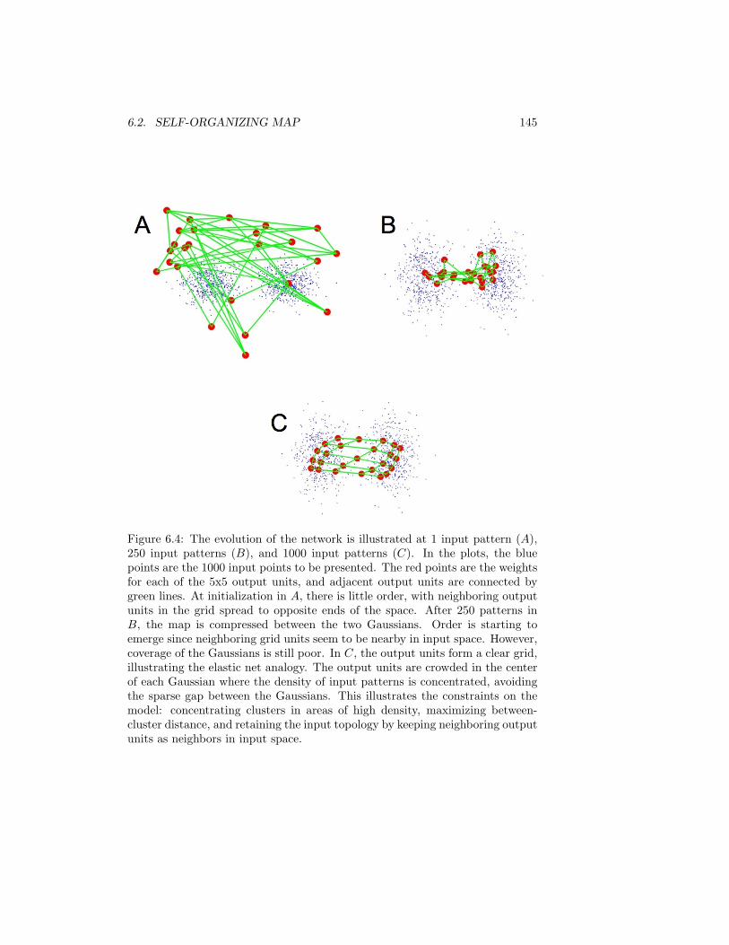
6.2. SELF-ORGANIZING MAP 145
Figure 6.4: The evolution of the network is illustrated at 1 input pattern (A),250 input patterns (B), and 1000 input patterns (C). In the plots, the bluepoints are the 1000 input points to be presented. The red points are the weightsfor each of the 5x5 output units, and adjacent output units are connected bygreen lines. At initialization in A, there is little order, with neighboring outputunits in the grid spread to opposite ends of the space. After 250 patterns inB, the map is compressed between the two Gaussians. Order is starting toemerge since neighboring grid units seem to be nearby in input space. However,coverage of the Gaussians is still poor. In C, the output units form a clear grid,illustrating the elastic net analogy. The output units are crowded in the centerof each Gaussian where the density of input patterns is concentrated, avoidingthe sparse gap between the Gaussians. This illustrates the constraints on themodel: concentrating clusters in areas of high density, maximizing between-cluster distance, and retaining the input topology by keeping neighboring outputunits as neighbors in input space.

146 CHAPTER 6. COMPETITIVE LEARNING
% ---------------------------------------------[xwin, ywin] = ind2sub(net.pool(‘output’).geometry,net.pool(‘output’).winner);
% get the (x,y) coordinates of each output unit in% the grid, stored in vectors ri and rj% -------------------------------------------------[ri,rj]= ind2sub(net.pool(‘output’).geometry,(1:net.pool(‘output’).nunits));
% Gaussian function that distributes activation% amongst the neighbors of the winner, with% the spread parameter lrange% --------------------------------------------dist = ((xwin - ri) .^ 2 ) + ((ywin - rj) .^ 2);net.pool(‘output’).activation = exp(-dist ./...
(2*lrange^2));net.pool(‘output’).activation = net.pool(‘output’).activation ./...
(2*pi*lrange^2);end
After the activation values are determined for each of the units, the weightsare updated. In contrast with simple competitive learning, not just the winner’sweights are updated. Each of the output units is pulled towards the inputpattern in proportion to its activation and the learning rate. This is done withthe following routine:
function change_weights()
% get the weight matrix, which has dimensions [noutput x ninput]% --------------------------------------------------------------------wt = net.pool(‘output’).proj(1).weight;
% for each output unit, in proportion to the activation of that output unit,% adjust the weights in the direction of the input pattern% ---------------------------------------------------------------------for k =1 :size(wt,1)
wt(k,:) = wt(k,:) + (lrate .* (net.pool(‘output’).activation(k)*...(net.pool(‘input’).activation - wt(k,:))));
endnet.pool(‘output’).proj(1).weight = wt;end
6.2.4 Overview of Exercises
We provide an exercise with the SOM in the cl program, showing how the SOMcould be applied as a model of topographic maps in the brain and illustratingsome of the basic properties of SOMs.
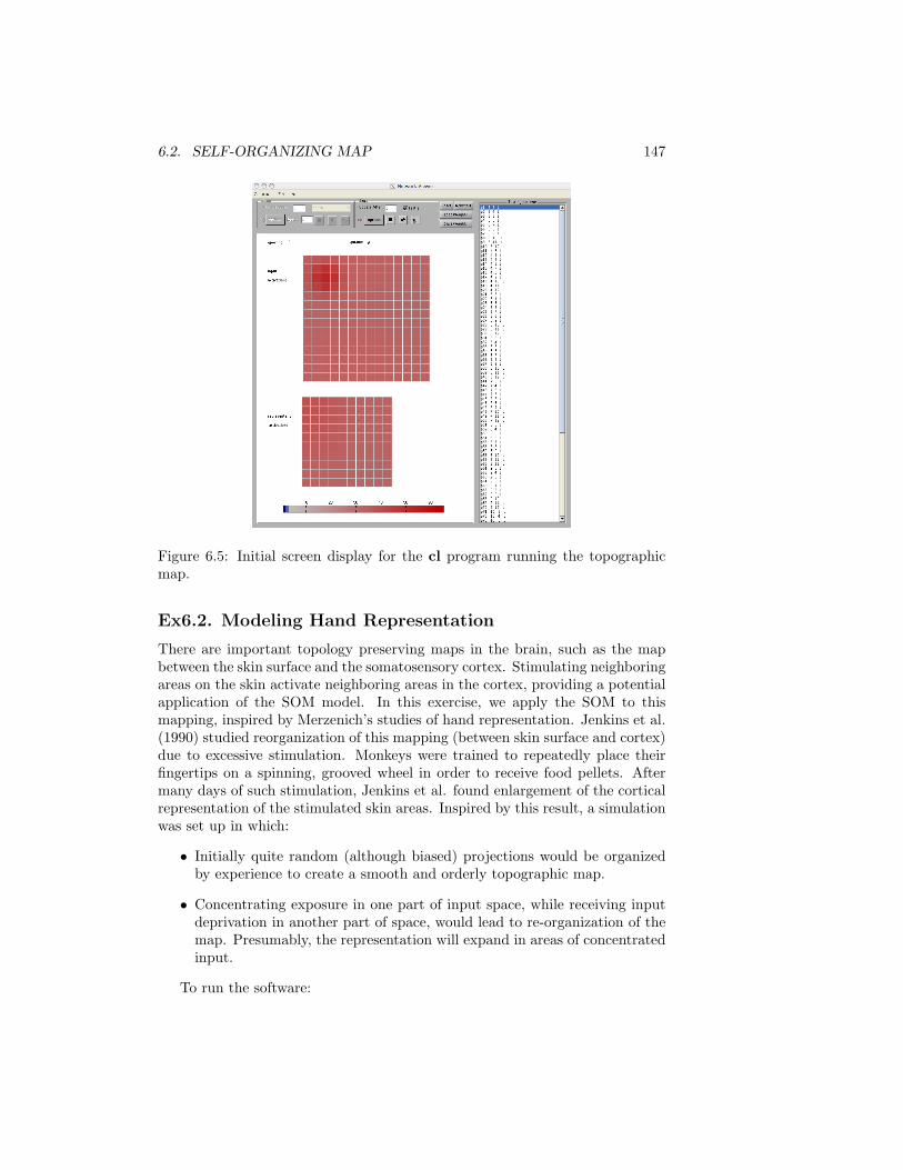
6.2. SELF-ORGANIZING MAP 147
Figure 6.5: Initial screen display for the cl program running the topographicmap.
Ex6.2. Modeling Hand Representation
There are important topology preserving maps in the brain, such as the mapbetween the skin surface and the somatosensory cortex. Stimulating neighboringareas on the skin activate neighboring areas in the cortex, providing a potentialapplication of the SOM model. In this exercise, we apply the SOM to thismapping, inspired by Merzenich’s studies of hand representation. Jenkins et al.(1990) studied reorganization of this mapping (between skin surface and cortex)due to excessive stimulation. Monkeys were trained to repeatedly place theirfingertips on a spinning, grooved wheel in order to receive food pellets. Aftermany days of such stimulation, Jenkins et al. found enlargement of the corticalrepresentation of the stimulated skin areas. Inspired by this result, a simulationwas set up in which:
• Initially quite random (although biased) projections would be organizedby experience to create a smooth and orderly topographic map.
• Concentrating exposure in one part of input space, while receiving inputdeprivation in another part of space, would lead to re-organization of themap. Presumably, the representation will expand in areas of concentratedinput.
To run the software:

148 CHAPTER 6. COMPETITIVE LEARNING
1. Start MATLAB, make sure the pdptool path is set, and change to thepdptool/cl directory.
2. At the MATLAB prompt, type “topo.” This will bring up two squarearrays of units, the upper one representing an input layer (like the skinsurface) and the lower one representing an internal representation (likethe cortical sheet) This window is displayed in Figure 6.5.
3. Start by running a test to get your bearings. Note that there are trainingand testing windows, train on the left and testing on the right. To test,click the selector button next to ‘options’ under test. Then select test all(so that it is checked) and click run.
The program will step through 100 input patterns, each producing a blobof activity at a point in the input space. The edges of the input space are usedonly for the flanks of the blobs, their centers are restricted to a region of 10x10units. The centers of the blobs will progress across the screen from left to right,then down one row and across again, etc. In the representation layer you willsee a large blob of activity that will jump around from point to point based onthe relatively random initial weights (more on this in Part 3).
Note that the input patterns are specified in the pattern file with a name,the letter x, then three numerical entries. The first is the x position on theinput grid (patx), the second is the y position (paty), and the third is a spreadparameter (σ), determining the width (standard deviation) of the Gaussianblob. All spreads have been set to 1. The activation of an input unit i, at gridcoordinates (ix,iy), is determined by:
activei =1
2πσ2e−12σ2 ((ix−patx)2+(iy−paty)2) (6.4)
which is the same Gaussian function (Equation 6.2) that determines the outputactivations, depending on the winning unit’s grid position.
The pool structure of the network is as follows:
Pool(1) is not used in this model.Pool(2) is the input pool.Pool(3) is the representation pool.
There is only one projection in the network, net.pool(3).proj(1), which containsthe weights in the network.
Part 1: Training the Network
Now you are ready to try to train the network. First, type “net.pool(3).lrange= 2.8” in the Command Window, to set the output activation spread to beinitially wide.
To begin training, select the training panel (click the button next to optionsunder train). The network is set up to run 200 epochs of training, with a learningrate (lrate) of .1. The “ptrain” mode is set, meaning that you will be training

6.2. SELF-ORGANIZING MAP 149
the network with the patterns presented in a randomly permuted order withineach epoch (each pattern is presented once per epoch). The display will updateonce per epoch, showing the last pattern presented in the epoch in the display.You can reduce the frequency of updating if you like to, say, once per 10 or 20epochs in the update after window.
Now if you test again, you may see some order beginning to emerge. That is,as the input blob progresses across and then down when you run a test all, theactivation blob will also follow the same course. It will probably be jerky andcoarse at the point, and sometimes the map comes out twisted. If it is twistedat this stage it is probably stuck.
If it is not twisted, you can proceed to refining the map. This is done bya process akin to annealing, in which you gradually reduce the lrange variable.A reasonable choice reducing it every 200 epochs of training in the followingincrements: 2.8 for the first 200 epochs, 2.1 for the second 200 epochs, 1.4 forthe third 200 epochs, and 0.7 for the last 200 epochs. So, you’ve trained for 200epochs as lrange = 2.8, so set “net.pool(3).lrange = 2.1.”
Then, run 200 more epochs (just click run) and test again. At this stage thenetwork seems to favor the edges too much (a problem that lessens but oftenremains throughout the rest of training). Then set net.pool(3).lrange to 1.4 atthe command prompt; then run another 200 epochs, then test again, then setit to 0.7, run another 200, then finally test again.
You may or may not have a nice orderly net at this stage. To get a sense ofhow orderly, you can log your output in the following manner. In test options,click “write output” then “set write options.” Click “start new log” and usethe name “part1 log.mat.” Click “Save” and you will return to the set writeoutput panel. In this panel, go into network variables, click net, it will open,click pool(3), it will open, click “winner” in pool(3), then click “add.” Theline “pool(3).winner” will then appear under selected. Click “OK.” NOTE: youmust also click OK on the Testing options popup for the log to actually beopened for use.
Now run a test again. The results will be logged as a vector showing thewinners for each of the 100 input patterns. At the MATLAB command windowyou can now load this information into MATLAB:
mywinners = load(‘part1_log’);
Then if you type (without forgetting the transpose operator ’):
reshape(mywinners.pool3_winner,10,10)’
you will get a 10x10 array of the integer indexes of the winners in your commandwindow. The numbers in the array correspond to the winning output unit. Theoutput unit array (the array of colored squares you see on the gui) is columnmajor, meaning that you count vertically 1-10 first and then 11 starts from thenext column, so that 1, 11, 21, 31, 41 etc. are on the same horizontal line. Inthe matrix printed in your command window, the spatial position correspondsto position of the test pattern centers. Thus, a perfect map will be numbered

150 CHAPTER 6. COMPETITIVE LEARNING
down then across such that it would have 1-10 in the first column, 11-21 in thesecond column, etc.
1 11 21 31 . . .2 12 22 32 . . .3 13 23 33 . . .4 14 24 34 . . ....
......
......
** The above array is your first result. Bring this (in printed form) to class fordiscussion. If your results are not perfect, which is quite likely, what is “wrong”with yours?
NOTE: The log currently stays open and logs all subsequent tests until youshut it off. To do this, click “test options” / “set write options” / and the click“log status off.” You should probably start a new log file each time you wantto examine the results, since the contents of the log file will require parsingotherwise. Also the file will then be available to reload and you can examine itscontents easily.
Part 2: Changing the seed
The results depend, as in the necker cube, on the value of the random seed. Trythe network again with a seed that works pretty well. Go to the very top left ofthe network viewer, click “set seed,” enter “211579,” then click ok. Then in theupper right find “Reset” and click that. Just setting the seed does not reset theweights. You must click “Reset.” Note that “Reset” resets the system withoutchanging the seed; if you click “Newstart” you will get a different seed.
To save time during training, we have provided a script to automate theprocess of reducing the lrange parameter. It is provided in “auto som.m,” andis run by typing “auto som” in the command prompt.
After training, save your weights after training, for the purposes of Part 4.To do this, click on the “Save weights” button in the upper right of the window.You will load these weights later in this exercise, so remember the folder andname you chose.
After training, the results should be pretty good. Go through the loggingsteps above, call your log file “part2 log.mat,” and display your results.
**The above array is your second result. Bring this also to class for discus-sion.
Part 3: Topographic bias in the initial weights
The neighborhood function causes the winning output unit and its neighbors tomove their weights in the same direction, developing the property that neigh-boring output units respond to similar stimuli. However, for the input gridto align properly with the output grid, there must be some underlying topo-graphic bias in the initial weights. Otherwise, the neighborhood function might

6.2. SELF-ORGANIZING MAP 151
help create an orderly response grid, but rotated 90 degrees, twisted, or perhapsworse, a jumbled mess. We will explore this initial topographic weight bias inthis exercise.
Note that when the network is initialized, the weights are assigned accordingto the explanation below:
Create a set of weights, weight rand(r,i), which are drawn randomlyfrom a uniform distribution from 0 to 1. Then, normalize the weightssuch that
sum(weight_rand(r,:)) = 1
for any output unit r.
Create a set of weights, weight topo(r,i), such that
weight_topo(r,i) = exp(-d/(2*net.pool(i).proj(j).ispread^2)) ..../ (2*pi*net.pool(i).proj(j).ispread^2)
where ‘d’ is the distance between unit r and unit i in their respectivegrids (aligned such that the middle 10x10 square of the input gridaligns with the 10x10 output grid). Thus, the weights have a Gaus-sian shape, such that the input units connect most strongly withoutput units that share a similar position in their respective grids.Also,
sum(weight_topo(r,:)) = 1 %approximately
due to the Gaussian function.
Then set the initial weights to:
net.pool(3).proj(1).weight(r,i) =(1. - topbias).* weight_rand(r,i) +topbias .* weight_topo(r,i);
Note that if topbias is 0 there is no topographic bias at all in the initialweights, and the weights are random. On the other hand if topbias is 1 theweights are pre-initialized to have a clear topographic (Gaussian) shape, gov-erned by standard deviation “ispread” (stands for “initial spread of weights”).These parameters are associated with net.pool(3).proj(1), and their values are:
% we make the problem hard initially!net.pool(3).proj(1).topbias = .1
% One standard deviation of the Gaussian covers 4 units,% so there’s an initially wide spread of the connections.net.pool(3).proj(1).ispread = 4
Q.6.2.1.

152 CHAPTER 6. COMPETITIVE LEARNING
Set net.pool(3).proj(1).topbias = 1 in the MATLAB console andclick “reset,” and then run through the test patterns without anytraining. How is the network responding, and why is this the case?Be brief in your response, and there is no need to log the result.
Q.6.2.2.
Set net.pool(3).proj(1).topbias = 0 in the MATLAB console, set theseed to 211579 (as in Part 2), and click “reset.” Now, run the stan-dard training regimen (the auto som.m file). How is the networkresponding? Do some adjacent input patterns activate adjacent re-sponse units?
** Bring these printed answers to class.
Part 4: Map reorganization through modified stimulation
The purpose of Part 4 is to demonstrate that after the map reaches a reasonableand stable organization, the map can be reorganized given a different distribu-tion of inputs, like the monkey finger tips in Jenkins et al. (1990), with expandedrepresentation in areas of high stimulation.
In this final part of the homework, a developed map will be selectively stim-ulated in the bottom half of the input space, receiving no input in the upperhalf. This, of course, is not analogous to the experiment, since the monkeyswould also receive stimulation in other areas of the hand not in contact withthe wheel. This exercise is rather a simplification to suggest how reorganizationis possible in the SOM.
First, load the weights for the trained network that you saved in Part 2. Dothis by clicking the Load weights button and select your saved weights. Afterthe weights are loaded, do a test cycle to ensure that the map is already trained.
After this, go into training options. Where it says Pattern file: Click “Loadnew.” Select “topo half.pat.” In case you want to switch the patterns back,topo.pat is the standard pattern file that you have been using.
Set net.pool(3).lrange = 0.7, and train the network for 400 epochs. Aftertraining, test the network. Changing the patterns before only applies to thetraining set, and you will want to change the test patterns as well. Thus, goto test options, and click “Load New,” and select topo half.pat. Also, start anew test log as described in Part 1 and create the log “part4 log.mat.” Testthe patterns and observe how the network now responds to this selected set oflower-half test patterns. Then type (without forgetting the transpose operatorafter the second line):
mywinners = load(‘part4_log’);reshape(mywinners.pool3_winner,10,5)’
This grid corresponds to only the winners for the bottom 50 input patterns.The first row was most telling of the reorganization. Compare it with the 6throw of your saved array from Part 2. The perfect map in Part 2 would have this

6.2. SELF-ORGANIZING MAP 153
row numbered 6, 16, 26, . . . , 96. If the ones digits in the row are numbers otherthan 6, this would be indicative of reorganization. Specifically, if the ones digitsare 4 or 5, that means the representation of this input row has creeped upwards,taking over territory that would previously have responded to the upper half ofthe patterns.
** This array is your third result. Bring this also to class for discussion.NOTE: You can either test with the same patterns you train with, or with
the original set of 100 patterns. The program generally allows different sets ofpatterns for training and testing.

154 CHAPTER 6. COMPETITIVE LEARNING

Chapter 7
The Simple RecurrentNetwork: A Simple Modelthat Captures the Structurein Sequences
Since the publication of the original pdp books (Rumelhart et al., 1986; Mc-Clelland et al., 1986) and backpropagation algorithm, the bp framework hasbeen developed extensively. Two of the extensions that have attracted the mostattention among those interested in modeling cognition have been the SimpleRecurrent Network (SRN) and the recurrent backpropagation (RBP) network.In this and the next chapter, we consider the cognitive science and cognitiveneuroscience issues that have motivated each of these models, and discuss howto run them within the PDPTool framework.
7.1 BACKGROUND
7.1.1 The Simple Recurrent Network
The Simple Recurrent Network (SRN) was conceived and first used by JeffElman, and was first published in a paper entitled Finding structure in time(Elman, 1990). The paper was ground-breaking for many cognitive scientistsand psycholinguists, since it was the first to completely break away from aprior commitment to specific linguistic units (e.g. phonemes or words), and toexplore the vision that these units might be emergent consequences of a learningprocess operating over the latent structure in the speech stream. Elman hadactually implemented an earlier model in which the input and output of thenetwork was a very low-level spectrogram-like representation, trained using aspectral information extracted from a recording of his own voice saying ‘This is
155

156CHAPTER 7. THE SIMPLE RECURRENT NETWORK: A SIMPLE MODEL THAT CAPTURES THE STRUCTURE IN SEQUENCES
Figure 7.1: The SRN network architecture. Each box represents a pool of unitsand each forward arrow represents a complete set of trainable connections fromeach sending unit to each receiving unit in the next pool. The backward arrow,from the hidden layer to the context layer denotes a copy operation. To see howthis architecture is represented in the PDPTool implementation, see Figure 7.7.Reprinted from Figure 2, p. 163, of Servan-Schreiber et al. (1991).
the voice of the neural network’. We will not discuss the details of this network,except to note that it learned to produce this utterence after repeated training,and contained no explicit feature, phoneme, syllable, morpheme, or word-levelunits.
In Elman’s subsequent work he stepped back a little from the raw-stimulusapproach used in this initial unpublished simulation, but he retained the funda-mental commitment to the notion that the real structure is not in the symbols weas researchers use but in the input stream itself. In Finding structure in time,Elman presented several simulations, one addressing the emergence of wordsfrom a stream of sub-lexical elements (he actually used the letters making upthe words as the elements for this), and the other addressing the emergence ofsentences from a stream of words. In both models, the input at any given timeslice comes from a small fixed alphabet; interest focuses on what can be learnedin a very simple network architecture, in which the task posed to the network isto predict the next item in the sting, using the item at time t, plus an internalrepresentation of the state of a set of hidden units from the previous time step.
An SRN of the kind Elman employed is illustrated in Figure 7.1. We actuallyshow the network used in an early follow-up study by Servan-Schreiber et al.(1991), in which a very small alphabet of elements is used (this is the particularnetwork provided with the PDPTool software, and it will be described in moredetail later).
The beauty of the SRN is its simplicity. In fact, it is really just a three-layer,feed-forward backpropagation network. The only proviso is that one of the twoparts of the input to the network is the pattern of activation over the network’s

7.1. BACKGROUND 157
own hidden units at the previous time step.In Elman’s simulations, input to the network consisted of an unbroken stream
of tokens from the alphabet. The simulation starts with small random connec-tion weights in all feed-forward projections. The first token in the stream ispresented, typically setting the values of the units in the input layer to a pat-tern of ones and zeros. Activation is propagated forward, as in a standardfeed-forward backpropagation network. The teaching input or target patternfor the output layer is simply the next item in the stream of tokens. The outputis compared to the target, delta terms are calculated, and weights are updatedbefore stepping along to the next item in the stream. Localist input and outputpatterns are often used in SRN’s, because this choice makes it easy from themodeler to understand the network’s output, as we shall see later. However,success at learning and discovery of useful and meaningful internal representa-tions does not depend on the use of localist input and output representations,as Elman showed in several of his simulations.
After processing the first item in the stream, the critical step—the one thatmakes the SRN a type of recurrent network—occurs. The state of the hiddenunits is ‘copied back’ to the context units, so that it becomes available as part ofthe input to the network on the next time step. The arrow labeled ‘copy’ in thefigure represents this step. Perhaps it is worth noting that this copy operationis really just a conceptual convenience; one can think of the context units assimply providing a convenient way of allowing the network to rely on the stateof the hidden units from the previous time step.
Once the copy operation is completed, the input sequence is stepped forwardone step. The input now becomes the item that was the target at the previoustime step, and the target now becomes the next item in the sequence. Activationis propagated forward, the output is compared to the target, delta terms arecalculated via backpropagation, and weights are updated. Note that the weightsthat are updated include those from the context (previous hidden state) to thehidden units (current hidden state). This allows the network to learn, not onlyto use the input, but also to use the context, to help it make predictions.
In most of Elman’s investigations, he simply created a very long streamof tokens from the alphabet, according to some generative scheme, and thenrepeatedly swept through it, wrapping around to the beginning when he reachedthe end of the sequence. After training with many presentations, he stoppedtraining and tested the network.
Here we briefly discuss three of the findings from Elman (1990). The firstrelates to the notion of ‘word’ as linguistic unit. The concept ‘word’ is actuallya complicated one, presenting considerable difficulty to anyone who feels theymust decide what is a word and what is not. Consider these examples: ‘linedrive’, ‘flagpole’, ‘carport’, ‘gonna’, ‘wanna’, ‘hafta’, ‘isn’t’ and ‘didn’t’ (oftenpronounced “dint”). How many words are involved in each case? If more thanone word, where are the word boundaries? Life might be easier if we did nothave to decide where the boundaries between words actually lie. Yet, we haveintuitions that there are points in the stream of speech sounds that correspondto places where something ends and something else begins. One such place

158CHAPTER 7. THE SIMPLE RECURRENT NETWORK: A SIMPLE MODEL THAT CAPTURES THE STRUCTURE IN SEQUENCES
Figure 7.2: Root mean squared error in predicting each of the indicated lettersfrom Elman’s letter-in-word prediction experiment. The letters shown are thefirst 55 letters in the text used for training the network. Reprinted from Figure6, p. 194, of Elman (1990).
might be between ‘fifteen’ and ‘men’ in a sentence like ‘Fifteen men sat down ata long table’, although there is unlikely to be a clear boundary between thesewords in running speech.
Elman’s approach to these issues, as previously mentioned, was to breakutternances down into a sequence of elements, and present them to an SRN. Inhis letter-in-word simulation, he actually used a stream of sentences generatedfrom a vocabulary of 15 words. The words were converted into a stream ofelements corresponding to the letters that spelled each of the words, with nospaces. Thus, the network was trained on an unbroken stream of letters. Afterthe network had looped repeatedly through a stream of about 5,000 elements,he tested its predictions for the first 50 or so elements of the training sequence.The results are seen in Figure 7.2.
What we see is that the network tends to have relatively high prediction errorfor the first letter of each word. The error tends to drop throughout the word,and then suddenly to shoot up again at the first letter of the next word. Thisis not always true – sometimes, afer a few downward steps, there is an uptickwithin a word, but such uptics generally correspond to places where there might
7.1. BACKGROUND 159
be the end of what we ordinarily call a word. Thus, the network has learnedsomething that corresponds at least in part with our intuitive notion of ‘word’,without building in the concept of word or ever making a categorical decisionabout the locations of word boundaries.
The other two findings come from a different simulation, in which the ele-ments of the sequences used corresponded to whole words, strung together againto form simple sentences. The set of words Elman used corresponded to sev-eral familiar nouns and verbs. Each sentence involved a verb, and at least onenoun as subject, with an optional subsequent noun as direct object. Verbs andnouns fell into different sub-types, – there were, for example, verbs of perception(which require an animate subject but can take any noun as object) and verbsof consumption, which require something consumable, and verbs of descruction,each of which had different restrictions on the nouns that could occur with itas subject and object. Crucially, the input patterns representing the nounsand verbs were randomly assigned, and thus did not capture in any way thecoocurrence structure of the domain. Over the course of learning, however, thenetwork came to assign each input its own internal representation. In fact, thehidden layer reflected both the input and the context; as a result, the patternsthe network learned to assign provided a highly context-sensitive form of lexicalrepresentation.
The next two figures illustrate findings from this simulation. The first ofthese (Figure 7.3) shows a cluster analysis based on the average pattern overthe hidden layer assigned to each of the different words in the corpus. What wesee is that the learned average internal representations indicate that the networkhas been able to learn the category structure and even the sub-category structureof the “lexicon” of this simple artificial language. The reason for this is largelythat the predictive consequences of each word correspond closely to the syntacticcategory and sub-category structure of the language. One may note, in fact,that the category structure encompasses distinctions that are usually treatedas syntactic (noun or verb, and within verbs, transitive vs intransitive) as wellas distinctions that are usually treated as semantic (fragile-object, food item),and at least one distinction that is clearly semantic (animate vs. inanimate)but is also often treated as a syntactically relevant “subcategorization feature”in linguistics. The second figure (Figure 7.4) shows a cluster analysis of thepatterns assigned two of the words (BOY and GIRL) in each of many differentcontexts. The analysis establishes that the overall distinction between BOYand GIRL separates the set of context-sensitive patterns into two highly similarsubtrees, indicating that the way context shades the representation of BOY issimilar to the way in which it shades the representation of GIRL.
Overall, these three simulations from Elman (1990) show how both segmen-tation of a stream into larger units and assignment of units into a hierarchicalsimilarity structure can occur, without there actually being any enumerated listof units or explicit assignment to syntactic or semantic categories.
Elman continued his work on SRN’s through a series of additional impor-tant and interesting papers. The first of these (Elman, 1991) explored thelearning of sentences with embedded clauses, illustrating that this was possible
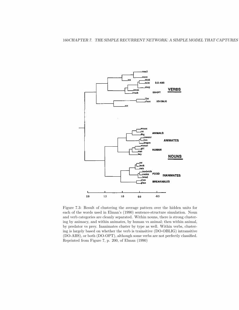
160CHAPTER 7. THE SIMPLE RECURRENT NETWORK: A SIMPLE MODEL THAT CAPTURES THE STRUCTURE IN SEQUENCES
Figure 7.3: Result of clustering the average pattern over the hidden units foreach of the words used in Elman’s (1990) sentence-structure simulation. Nounand verb categories are cleanly separated. Within nouns, there is strong cluster-ing by animacy, and within animates, by human vs animal; then within animal,by predator vs prey. Inanimates cluster by type as well. Within verbs, cluster-ing is largely based on whether the verb is trainsitive (DO-OBLIG) intransitive(DO-ABS), or both (DO-OPT), although some verbs are not perfectly classified.Reprinted from Figure 7, p. 200, of Elman (1990)

7.1. BACKGROUND 161
Figure 7.4: Hierarchical cluster diagram of hidden unit activation vectors inresponse to some occurrences of the inputs BOY and GIRL. Upper-case labelsindicate the actual input; lowercase labels indicate the context. Note in bothcases the large cluster in the middle corresponding to BOY or GIRL as subject,and the large clusters flanking these above and below correponding primarily tocases in which BOY or GIRL is the sentential object. Reprinted from Figure 9,p. 206, from Elman (1990).

162CHAPTER 7. THE SIMPLE RECURRENT NETWORK: A SIMPLE MODEL THAT CAPTURES THE STRUCTURE IN SEQUENCES
in this simple network architecture, even though the network did not rely onthe computational machinery (an explicitly recursive computational structure,including the ability to ‘call’ a computational process from within itself) usuallythought to be required to deal with imbeddings. A subsequent and highly influ-ential paper (Elman, 1993) reported that success in learning complex embeddedstructures depended on starting small – either starting with simple sentences,and gradually increasing the number of complex ones, or limiting the network’sability to exploit context over long sequences by clearing the context layer afterevery third element of the training sequence. However, this later finding waslater revisited by Rohde and Plaut (1999). They found in a very extensive seriesof investigations that starting small actually hurt eventual performance ratherthan helped it, except under very limited circumstances. A number of othervery interesting investigations of SRN’s have also been carried our by Taborand collaborators, among other things using SRN’s to make predictions aboutparticipants reading times as they read word-by-word through sentences (Taboret al., 1997).
7.1.2 Graded State Machines
The simple recurrent network introduced by Elman (1990) also spawed inves-tigations by Servan-Schreiber et al. (1991). We describe this work in greaterdetail than some of the other work following up on Elman (1990) because theexercise we provide is based on the Servan-Schreiber et al. (1991) investigations.
These authors were especially interested in exploring the relationship be-tween SRNs an classical automata, including Finite State Transition Networks,and were also interested in the possibility that SRNs might provide useful mod-els of implicit sequence learning in humans (Cleeremans and McClelland, 1991).Servan-Schreiber et al. (1991) investigated the learning of sequences that couldbe generated by a simple finite-state transition network grammar of the kindused to generate stimuli used in human implicit learning experiments by Rebur(1976), and illustrated in Figure 7.5. Sequence generation occurs as follows.Each sequence begins with the symbol ‘B’, and enters the state associated withthe node in the diagram marked ‘#0’. From there, a random choice is made tofollow one of the two links leading out of node 0. After the random choice, thesymbol written beside the link is added as the second element of the sequence,and the process transitions to the state at the end of the chosen link. The choicecould, for example, be the upper link leaving node 0, producing a T and shiftingto node 1. The process iterates as before, choosing one of two links out of thecurrent node, adding the symbol written next to the link as the next elementof the seqeuence, and shifting to the node at the end of the link. When node 5is reached, there is only one remaining possibility; the symbol E is written, andthe sequence then ends.
In their simulation of learning sequences generated by the Finite State Tran-sition Network, Servan-Schreiber et al. (1991) assumed that the learner is trainedwith a series of sequences, which may be generated at random by the sequence-generating finite-state transition network. At the beginning of each sequence,

7.1. BACKGROUND 163
Figure 7.5: The stochastic finite-state transition network used in the gsm sim-ulation. Strings are generated by transintioning between nodes connected bylinks, and emitting the symbol associated with each link. Where two links leavethe same node, one is chosen at random with equal probability. Reprinted fromFigure 3, p. 60, of Servan-Schreiber et al. (1991), based on the network usedearlier by Rebur (1976).
the context representation is reset of a neutral initial state, and the initial ele-ment B is presented on the input. The network then tries to predict the nextelement of the sequence, which then is presented as the target. Small adjust-ments to the weights are made, and then the process steps forward through thesequence. Now the second element of the sequence (the one after the B) is pre-sented at the the input, and the third item in the sequence becomes the target.The process of propagating activation forward, adjusting the the connections,and stepping forward to the next element continues, until the last element of thesequence (the E symbol) is reached. At that point, processing of the sequenceends. The process then begins again with the next sequence.
In their paper, Servan-Schreiber et al. (1991) demonstrated that a networklike the one shown in Figure 7.1 could essentially learn to become the transi-tion network grammar through a completely gradual and continuous learningprocess. That is, as a result of training, the patterns at the hidden layer cameto correspond closely to the nodes of the finite state transition network, in thesense that there was essentially one hidden pattern corresponding to each ofthe nodes in the network, regardless of the sequence of elements leading to thatnode. However, the network could also learn to ‘shade’ its representation ofeach node to a certain extent with the details of the prior context, so that itwould eventually learn to capture subtle idiosyncratic constraints when trainedrepeatedly on a fixed corpus of legal example sentences. The authors also wenton to show that the network could learn to use such subtle shading to carryinformation forward over an embedded sequence, but this will only happen inthe SRN if the material needed at the end of the embedding is also of some

164CHAPTER 7. THE SIMPLE RECURRENT NETWORK: A SIMPLE MODEL THAT CAPTURES THE STRUCTURE IN SEQUENCES
relevance within the sequence.The reader is referred to the paper by Servan-Schreiber et al. (1991) for
further details of these investigations. Here we concentrate on describing thesimulation model that allows the reader to explore the SRN model, using thesame network and one of the specific training sets used by Servan-Schreiberet al. (1991).
7.2 THE SRN PROGRAM
The srn is a specific type of backpropagation network. It assumes a feed-forwardarchitecture, with units in input, hidden, and output pools. It also allows fora special type of hidden layer called a “context” layer. A context layer is ahidden layer that receives a single special type of projection from another layercontaining the same number of units, typically a hidden layer. This special typeof projection (called a ‘copy-back projection’) allows the pattern of activationleft over on the sending units from the last input pattern processed to be copiedonto the receiving units for use as context in processing the next input pattern.
7.2.1 Sequences
The srn network type’s environment provides a construct called “sequences”,which consists of one or more input-output pairs to be presented in a fixed order.
The idea is that one might experience a series of sequences, such that eachsequence has a fixed structure, but the order in which the sequences appear canbe random (permuted) within each epoch. In the example provided, a sequenceis a sequence of characters beginning with a B and ending with an E.
Sequences can be defined in the pattern file in two different ways:
Default The default method involves beginning the specification of each se-quence with a name, followed by a series of input-output pairs, followedby ‘end’ (see the file srn gsm21.pat for an example). When the file isread, a data structure element is created for the sequence and added tothe sequences structure, itself a property of the network’s environment.At the beginning of each sequence, the state of the context units is initial-ized to all .5’s at the same time that the first input pattern is presented onthe input. At each successive step through the sequence, the state of thecontext units is equal to the state of the hidden units determined duringthe previous step in the sequence.
SeqLocal The SeqLocal method of specifying a sequence works only for a re-stricted class of possible cases. These are cases where (a) each input andtarget pattern involves a single active unit; all other inputs and targetsare 0; and (b) the target at step n is the input at step n+1 (except forthe last element of the sequence). For such cases, the .pat file must beginwith a line like this:

7.2. THE SRN PROGRAM 165
SeqLocal b t s x v p e
This line specifies that the following entries will be used to construct actualinput output pattern pairs, as follows. The character strings followingSeqLocal are treated as labels for both the input and output units, withthe first label being used for the first input unit and the first output unitetc. Single characters are used in the example but strings are supported.
Specific sequences are then specified by lines like the following:
p05 b t x s e
Here each line begins with a pname, followed by a series of instances ofthe different labels previously defined. The case shown above generatesfour input-output pattern pairs; the first input contains a 1 in the firstposition and 0’s elsewhere and the first target contains a 1 in the secondposition and 0’s elsewhere. The second input is the same as the first target,etc. Thus, in this model the user specifies the actual symbolic trainingsequences and these are translated into actual input and output patternsfor the user.
Using the last target from the previous sequence as the first element ofthe input for the next sequence. If the first label in the string of labels isthe special label ‘#’, the last target pattern from the previous sequenceis used as the first input pattern for the current sequence. In this case,we also copy the state of the hidden units from the network’s predictionof the last target to the context layer, instead of resetting the context tothe clearval.
7.2.2 New Parameters
mu The srn program introduces one new parameter called mu, which is a fieldunder train options. This parameter specifies a scale factor used to de-termine how large a fraction of the pattern of activation from the contextlayer at time step n is added to the pattern copied back from the hiddenlayer. In the gsm simulation, mu is set to 0. Non-zero values of mu forcesome trace of the earlier context state to stick around in the current stateof the context units.
clearval At the beginning of each training and testing sequence, the activationsof the context units are set to the value of this parameter, representedas clear value in the train and test options windows. By default, thisparameter is set to .5. If a negative value is given, the states of the unitsare not reset at the beginning of a new sequence; instead the state fromthe last element of the preceding sequence is used.

166CHAPTER 7. THE SIMPLE RECURRENT NETWORK: A SIMPLE MODEL THAT CAPTURES THE STRUCTURE IN SEQUENCES
7.2.3 Network specification
The .m file specifies the specific architecture of the model as in other PDPtoolprograms. To have a pool of units treated as a ‘context’ layer, it should be oftype ‘copyback’ and should receive a single projection from some other layer(typically a hidden layer) which has its constraint type field set to ‘copyback’.When the constraint type is ‘copyback’, there are no actual weights, the stateof the ‘sending’ units is simply copied to the ‘receiving’ units at the same timethat the next target input is applied (except at the beginning of a new sequence,where the state of each of the context units is set to the clearval, which by defaultis set to .5).
7.2.4 Fast mode for training
The srn program’s inner loops have been converted to fast mex code (c codethat interfaces with MATLAB). To turn on the fast mode for network training,click the ’fast’ option in the train window. This option can also be set by typingthe following command on the MATLAB command prompt:runprocess(’process’,’train’,’granularity’,’epoch’,’count’,1,’fastrun’,1);
There are some limitations in executing fast mode of training.In this mode,network output logs can only be written at epoch level. Any smaller outputfrequency if specified, will be ignored.When running with fast code in gui mode,network viewer will only be updated at epoch level.Smaller granularity of displayupdate is disabled to speed up processing.
There is a known issue with running this on linux OS.MATLAB processesrunning fast version appear to be consuming a lot of system memory. Thismemory management issue has not been observed on windows. We are currentlyinvestigating this and will be updating the documentation as soon as we find afix.
7.3 EXERCISES
The exercise is to replicate the simulation discussed in Sections 3 and 4 ofServan-Schreiber et al. (1991). The training set you will use is described inmore detail in the paper, but is presented here in Figure 7.6. This particularset contains 21 patterns varying in length from 3 to 8 symbols (plus a B at thebeginning and an E at the end of each one).
To run the exercise, download the latest version of pdptool, set your path toinclude pdptool and all of its children, and change to the pdptool/exercises/srnexercises directory. Type ‘srn gsm’ (standing for “Graded State Machine”) atthe MATLAB prompt. After everything loads you will see a display showing(at the right of the screen) the input, hidden and output units, and a vectorrepresenting the target for the output units (see Figure 7.7). To the left of theinput is the context. Within the input, output, and target layers the units arelaid out according to Figure 7.1. Your exercise will be to test the network after10, 50, 150, 500, and 1000 epochs of training. The parameters of the simulation

7.3. EXERCISES 167
Figure 7.6: The training patterns used in the gsm exercise. A B is added to thebeginning of each sequence and an E is added to the end in the gsm simulation.Reprinted from Figure 12, p. 173, of Servan-Schreiber et al. (1991).
are a little different from the parameters used in the published article (it is notclear what values were actually used in the published article in some cases), andthe time course of learning is a little extended relative to the results reportedin the paper, but the same basic pattern appears.
One thing to be clear about at the outset is that the training and testingis organized at the sequence level. Each sequence corresponds to a string thatcould be generated by the stochastic finite state automaton shown in Figure7.5. The ptrain option, ‘p’ (which is the one used for this exercise) permutesthe order of presentation of sequences but presents the elements of the sequencein its canonical sequential order. Each sequence begins with a B and ends withan E, and consists of a variable number N of elements. As described above, thesequence is broken down into N-1 input-target pairs, the first of which has a Bas input and the successor of B in the sequence as its target, and the last ofwhich has the next to last symbol as its input and E as its target. When theB symbol is presented, the context is reset to .5’s. It makes sense to updatethe display during testing at the pattern level, so that you can step throughthe patterns within each sequence. During training, update the display at theepoch level or after 10 epochs.
Before you begin, consider:
• What is the 0-order structure of the sequences? That is, if you had no ideaabout even the current input, what could you predict about the output?This question is answered by noting the relative frequency of the variousoutputs. Note that B is never an output, but all the other characters canbe outputs. The 0-order structure is thus just the relative frequency ofeach character in the output.
• What is the 1st order structure of the sequences? To determine this ap-proximately, consult the network diagram (last page of this handout) andnote which letters can occur after each letter. Make a little grid fouryourself of seven rows each containing seven cells. The row stands for thecurrent input, the cell within a row for a possible successor. So, consultingthe network diagram, you will find that B can be followed only by T or P .So, place an X in the second (T ) cell of the first row and the 6th (P ) cellof the first row. Fill in the rest of the rows, being careful to attend to the

168CHAPTER 7. THE SIMPLE RECURRENT NETWORK: A SIMPLE MODEL THAT CAPTURES THE STRUCTURE IN SEQUENCES
Figure 7.7: Network view showing the layout for the srn network.
direction of the arrows coming out of each node in the diagram and thelabel on each arc. You should find (unless I made a mistake) that three ofthe letters actually have the exact same set of possible successors. Checkyourself carefully to make sure you got this correct.
OK, now run through a test, before training. You should find that thenetwork produces near uniform output over the output units at each step oftesting.
NOTE: For testing, set update to occur after 1 pattern in the test window.Use the single step mode and, in this case, quickly step through, noticing howlittle the output changes as a function of the input. The weights are initializedin a narrow range, making the initial variation in output unit activation rathertiny. You can examine the activations of the output units at a given point bytyping the following to the MATLAB console:
net.pools(5).activation
When you get tired of stepping through, hit ‘run’ in the test window. Theprogram will then quickly finish up the test.
The basic goal of this exercise is to allow you to watch the network proceed tolearn about the 0th, 1st, and higher-order structure of the training set. You havealready examined the 0th and 1st order structure; the higher-order structure isthe structure that depends on knowing something about what happened beforethe current input. For example, consider the character V . What can occur aftera V , where the V is preceded by a T? What happens when the V is preceded

7.3. EXERCISES 169
by an X? By a P? By another V ? Similar questions can be asked about otherletters.
Q.7.0.3.
Set nepochs in the training options panel to ten, run ten epochs oftraining, then test again.
What would you say has been learned at this point? Explain youranswer by referring to the pattern of activation across the outputunits for different inputs and for the the same input at differentpoints in the sequence.
Continue training, testing after a total of 50, 150, 500, and 1000epochs. Answer the same question as above, for each test pointpoint.
Q.7.0.4.
Summarize the time course of learning, drawing on your results forspecific examples as well as the text of section 4 of the paper. How dothe changes in the representations at the hidden and context layerscontribute to this process?
Q.7.0.5.
Write about 1 page about the concept of the SRN as a graded statemachine and its relation to various types of discrete-state automata,based on your reading of the entire article (including especially thesection on spanning embedded sequences).
Try to be succinct in each of your answers. You may want to run the wholetraining sequence twice to get a good overall sense of the changes as a functionof experience.

170CHAPTER 7. THE SIMPLE RECURRENT NETWORK: A SIMPLE MODEL THAT CAPTURES THE STRUCTURE IN SEQUENCES

Chapter 8
RecurrentBackpropagation: Attractornetwork models of semanticand lexical processing
Recurrent backpropagation networks came into use shortly after the develop-ment of the backpropagation algorithm was first developed, and there are manyvariants of such networks. Williams and Zipser (1995) provide a thorough reviewof the recurrent backpropagation computational framework. Here we describe aparticular variant, used extensively in PDP models to study the effects of braininjury on lexical and semantic processing (Plaut and Shallice, 1993; Plaut et al.,1996; Rogers et al., 2004; Dilkina et al., 2008).
8.1 BACKGROUND
A major source of motivation for the use of recurrent backpropagation networksin this area is the intuition that they may provide a way of understandingthe pattern of degraded performance seen in patients with neuropsychologicaldeficits. Such patients make a range of very striking errors. For example, somepatients with severe reading impairments make what are called semantic errors– misreading APRICOT as PEACH or DAFFODIL as TULIP. Other patients,when redrawing pictures they saw only a few minutes ago, will sometimes puttwo extra legs on a duck, or draw human-like ears on an elephant.
In explaining these kinds of errors, it has been tempting to think of the pa-tient as having settled into the wrong basin of attraction in a semantic attractornetwork. For cases where the patient reads ‘PEACH’ instead of ‘APRICOT’,the idea is that there are two attractor states that are ‘near’ each other in asemantic space. A distortion, either of the state space itself, or of the mapping
171

172CHAPTER 8. RECURRENT BACKPROPAGATION: ATTRACTOR NETWORK MODELS OF SEMANTIC AND LEXICAL PROCESSING
Figure 8.1: Conceptual illustration of a semantic state-space containing basinsof attraction (solid ellipses) for CAT , COT . and BED. Distortion (dottedellipse) of the basin for COT can result in CAT falling into it. A differentdistortion, not shown, could allow COT to fall into the basin for BED. FromFigure 4 p. 394 of Plaut and Shallice (1993).
into that space, can result in an input that previously settled to one attractorstate settling into the neighboring attractor. Interestingly, patients who makethese sorts of semantic errors also make visual errors, such as misreading ‘cat’as ‘cot’, or even what are called ‘visual-then-semantic’ errors, mis-reading ‘sym-pathy’ as ‘orchestra’. All three of these types of errors have been capturedusing PDP models that rely on the effects of damage in networks containinglearned semantic attractors (Plaut and Shallice, 1993). Figure 8.1 from Plautand Shallice (1993) illustrates how both semantic and visual errors can occuras a result of damage to an attractor network that has learned to map fromorthography (a representation of the spelling of a word) to semantics (a repre-sentation of the word’s meaning), taking printed words and mapping them tobasins of attraction within a recurrent semantic network.
The use of networks with learned semantic attractors has an extensive his-tory in work addressing semantic and lexical deficits, building from the work ofPlaut and Shallice (1993) and other early work (Farah and McClelland, 1991;Lambon Ralph et al., 2001). Here we focus on a somewhat more recent modelintroduced to address a progressive neuropsychological condition known as se-

8.2. THE RBP PROGRAM 173
mantic dementia by Rogers et al. (2004). In this model, the ‘semantic’ represen-tation of an item is treated as an attractor state over an population of neuronsthought to be located in a region known as the ‘temporal pole’ or anterior tem-poral lobe. The neurons in this integrative layer receive input from, and projectback to, a number of different brain regions, each representing a different typeof information about an item, including what it looks like, how it moves, whatit sounds like, the sound of its name, the spelling of the word for it, etc. The ar-chitecture of the model is sketched in Figure 8.2 (top). Input coming to any oneof the visible layers can be used to activate the remaining kinds of information,via the bi-directional connections among the visible layers and the integrativelayer and the recurrent connections among the units in the integrative layer.According to the theory behind the model, progressive damage to the neuronsin the integrative layer and/or to the connections coming into and out of thisintegrative layer underlies the progressive deterioration of semantic and abilitiesin semantic dementia patients (?).
8.2 THE RBP PROGRAM
In the version of recurrent backpropagation that we consider here, activationsof units are thought of as being updated continuously over some number of timeintervals. The network is generally set to an initial state (corresponding to time0), in which some units are clamped to specific values by external inputs, whileothers are initialized to a default starting value. Processing then proceeds inwhat is viewed conceptually as a continuous process for the specified number oftime intervals. At any point along the way, target patterns can be provided forsome of the pools of units in the network. Typically, these networks are trainedto settle to a single final state, which is represented by a target to be matchedover a subset of the pools in the network, over the last few time intervals.
At the end of the forward activation process, error signals are “back propa-gated through time” to calculate delta terms for all units in the network acrossthe entire time span of the settling process. A feature of recurrent backprop-agation is that the same pool of units can have both external inputs (usuallyprovided over the first few time intervals) and targets (usually specified for thelast few intervals). These networks are generally thought of as settling to at-tractor states, in which there is a pattern of activation over several differentoutput pools. In this case, the target pattern for one of these pools might alsobe provided as the input. This captures the idea that I could access all aspectsof my concept of, for example, a clock, either from seeing a clock, hearing aclock tick, hearing or reading the word clock, etc.
One application of these ideas is in the semantic network model of Rogerset al. (2004). A schematic replica of this model is shown in Figure 8.2 (top).There are three sets of visible units, corresponding to the name of the object,other verbal information about the object, and the visual appearance of theobject. Whichever pattern is provided as the input, the task of the network is tosettle to the complete pattern, specifying the name, the other verbal information

174CHAPTER 8. RECURRENT BACKPROPAGATION: ATTRACTOR NETWORK MODELS OF SEMANTIC AND LEXICAL PROCESSING
about the object, and the visual percept. Thus the model performs patterncompletion, much like, for example, the Jets-and-Sharks iac model from Chapter2. A big difference is that the Rogers et al. (2004) model uses learned distributedrepresentations rather than instance units for each known concept.
8.2.1 Time intervals, and the partitioning of intervals intoticks
The actual computer simulation model, called rbp, treats time, as other net-works do, as a sequence of discrete steps spanning some number of canonicaltime intervals. The number of such intervals is represented by the variable nin-tervals. In rbp, the discrete time steps, called ticks, can slice the whole span oftime very finely or very coarsely, depending on the value of a parameter calleddt. The number of ticks per interval is 1/dt, and the total number of ticks ofprocessing is equal to nintervals/dt. The number of states of the network isone larger than the number of ticks; there is an initial state, at time 0, and astate at the end of each tick — so that the state at the end of tic 1 is state 1,etc.
8.2.2 Visualizing the state space of an rbp network
To understand the recurrent backpropagation network, it is useful to visualizethe states of all of the units in the network laid out on a series of planes, withone plane per state (Figure 8.2). Within each plane all of the pools of units inthe network are represented. Projections are thought of as going forward fromone plane to the next. Thus if pool(3) of a network receives a projection frompool(2), we can visualize nticks separate copies of this projection, one to theplane for state 1 from the plane for state 0, one to the plan for state 2 from theplan for state 2, etc.
8.2.3 Forward propagation of activation.
Processing begins after the states of all of the units have been initialized to theirstarting values for state 0. Actually, both the activations of units, and their netinputs, must be initialized. The net inputs are set to values that correspond tothe activation (by using the inverse logistic function to calculate the startingnet input from the starting activation). For cases where the unit is clamped at0 or 1, the starting net input is based on the correct inverse logistic value for2.0e-8 and 1-(2.0e-8). [CHECK]
After the net inputs and activations have been established for state 0, thenet inputs are calculated for state 1. The resulting net input value is essen-tially a running average, combining what we will call the newnet, based on theactivations at the previous tick with the old value of the net input:
newneti(t) = biasi + exti(t) +∑j
aj(t− 1)wij

8.2. THE RBP PROGRAM 175
Figure 8.2: Standard (top) and unfolded (bottom) visualization of a recurrentneural network like the one used in the Rogers et al. (2004) model. The unfoldednetwork makes clear the fact that activation at one time influences the activa-tions at the next time step. In this unfolded form, the network is equivalentto a feed-forward network, where forward refers now to time. Activation feedsforward in time, and error signals (delta terms) feed back.

176CHAPTER 8. RECURRENT BACKPROPAGATION: ATTRACTOR NETWORK MODELS OF SEMANTIC AND LEXICAL PROCESSING
neti(t) = dt ∗ newneti(t) + (1− dt) ∗ neti(t− 1)
Note that if dt = 1 (the largest allowable value), the net input is not timeaveraged, and net(t) simply equals newnet(t).
After net inputs for state t have been computed, activation values for statet are then computed based on each unit’s net input for state t. A variant onthis procedure (not available in the rbp simulator) involves using the newnetto calculate a newact value, and then time averaging is then applied on theactivations:
ai(t) = dt ∗ newacti(t) + (1− dt) ∗ ai(t− 1)
Time-averaging the net inputs is preferred because net input approximates aneuron’s potential while activation approximates its firing rate, and it is gener-ally thought that it is the potential that is subject to time averaging (‘temporalsummation’). Also, time-averaging the net input allows activation states tochange quickly if the weights are large. The dynamics seems more dampedwhen time-averaging is applied to the activations.
Once activation values have been computed, error measures and delta terms(called dEdA) are calculated, if a target has been specified for the given stateof the unit. The error is thought of as spread out over the ticks that make upeach interval over which the target is applied, and so the magnitude of the errorat each time step is scaled by the size of the time step. Either sum squarederror (sse) or cross entropy error (cee) can be used as the error measure whosederivative drives learning. In either case, we compute both measures of error,since this is fast and easy. The sse for a given unit at a given time step is
ssei(t) = dt ∗ (tgti(t)− ai(t))2,
where tgti(t) is the externally supplied target at tick t. The cce for a given unitat a given time step is
ccei(t) = −dt ∗ (tgti(t) ∗ log(ai(t)) + (1− tgti(t)) ∗ log(1− ai(t))) ,
In the forward pass we also calculate a quantity we will here call the ‘direct’dEdnet for each time step. This is that portion of the partial derivative of theerror with respect to the net input of the unit that is directly determined bythe presence of a target for the unit at time step t. If squared error is used, thedirect dEdnet is given by
directdEdneti(t) = (tgti(t)− ai(t)) ∗ ai(t) ∗ (1− ai(t))
Note that the direct dEdnet will eventually be scaled by dt, but this is appliedduring the backward pass as discussed below. Of course if there is no target thedirectdEdneti(t) is 0.
If cross-entropy error is used instead, we have the following simpler expres-sion, due to the cancellation of part of the gradient of the activation functionwith part of the derivative of the cross entropy error:
directdEdneti(t) = (tgti(t)− ai(t))

8.2. THE RBP PROGRAM 177
The process of calculating net inputs, activations, the two error measures, andthe direct dEdnet takes place in the forward processing pass. This processcontinues until these quantities have been computed for the final time step.
The overall error measure for a specific unit is summed over all ticks forwhich a target is specified:
ei =∑t∗ei(t)
This is done separately for the sse and the cce measures.The activations of each unit in each tick are kept in an array called the
activation history. Each pool of units keeps its own activation history array,which has dimensions [nticks+1, nunits]
8.2.4 Backward propagation of error
We are now ready for the backward propagation of the dEdnet values. Wecan think of the dEdnet values as being time averaged in the backwards pass,just as the net inputs are in the forward pass. Each state propagates back tothe preceding state, both through the time averaging and by backpropagationthrough the weights, from later states to earlier states:
dEdneti(t) = dt ∗ newdEdneti(t) + (1− dt) ∗ dEdneti(t+ 1),
where
newdEdneti(t) = ai(t)∗(1−ai(t))∗∑k
wki ∗dEdnetk(t+1)+directdEdneti(t).
The subscript k in the summation above indexes the units that receive connec-tions from unit i. Note that state 0 is thought of as immutable, so deltas neednot be calculated for that state. Note also that for the last state (the statewhose index is nticks + 1), there is no future to inherit error derivatives from,so in that case we simply have
dEdneti(nticks+ 1) = dt ∗ directdEdneti(nticks+ 1).
For the backward pass calculation, t starts at the next-to-last state (whose indexis nticks) and runs backward to t = 1; however, for units and ticks where theexternal input is hard clamped, the value of dEdnet is kept at 0.
All of the dEdneti(t) values are maintained in an array called dEdnethistory.As with the activations, there is a separate dEdnet history for each pool of units,which like the activation history array, has dimensions [nticks+1,nunits]. (Inpractice, the values we are calling directdEdnet scaled by dt and placed in thishistory array on the forward pass, and the contents of that array is thus simplyincremented during the backward pass).

178CHAPTER 8. RECURRENT BACKPROPAGATION: ATTRACTOR NETWORK MODELS OF SEMANTIC AND LEXICAL PROCESSING
8.2.5 Calculating the weight error derivatives
After the forward pass and the backward pass, we are ready to calculate theweight error derivatives arising from this entire episode of processing in thenetwork. This calculation is very simple. For each connection weight, we simplyadd together the weight error derivative associated with each processing tick.The weight error derivative for each tick is just the product of the activationof the sending unit from the time step on the input side of the tick times thedEdnet value of the receiving unit on the receiving side of the tick:
wedij =nticks+1∑t=1
dEdneti(t) ∗ aj(t− 1)
8.2.6 Updating the weights.
Once we have the weight error derivatives, we proceed exactly as we do in thebackpropagation algorithm as implemented in the bp program. As in standardbackpropagation, we can update the weights once per pattern, or once per Npatterns, or once per epoch. Patterns may be presented in sequential, or per-muted order, again as in the bp program. Momentum and weight decay canalso be applied.
8.3 Using the rbp program with the rogers net-work
Training and testing in rbp work much the same as in other networks. Therogers network has been set up in advance for you, and so you can launch theprogram to run the rogers example by simply typing rogers at the MATLABcommmand prompt while in the rbp directory. See Figure 8.3 for the screenlayout of this network.
During testing, the display can be updated (and the state of the networkcan be logged) at several different granularities: At the tick level, the intervallevel, and the pattern level. When tick level or interval level is specified, state0 is shown first, followed by the state at the end of the first tick or interval,until the end of the final tick is reached. The template for the rogers model,rogers.m, also displays the target (if any) associated with the state, below theactivations of each pool of units in the network. With updating at the patternlevel, the state is updated only once at the end of processing each pattern.
Backpropagation of error occurs only during training, although during train-ing the display update options are limited to the pattern and the epoch level.The user can log activations forward and deltas back at the tick level via the setwrite options button in the train options panel (select backtick for ‘frequency’of logging). Otherwise logging only occurs in the forward direction.

8.3. USING THE RBP PROGRAM WITH THE ROGERS NETWORK 179
Figure 8.3: Architecture of the Rogers et al. (2004) model. Verbal descriptors(names, perceptual, functional, and encyclopedic) and visual feature units re-ceive input directly from the environment. The environmental input is displayeddirectly below the corresponding pool activations.

180CHAPTER 8. RECURRENT BACKPROPAGATION: ATTRACTOR NETWORK MODELS OF SEMANTIC AND LEXICAL PROCESSING
8.3.1 rbp fast training mode.
A great deal of computing is required to process each pattern, and thus ittakes quite a long time to run one epoch in the rbp program. To amelioratethis problem, we have implemented the pattern processing steps (forward pass,backward pass, and computing the weight error derivatives) within a ‘mex’ file(essentially, efficient C code that interfaces with MATLAB data formats andstructures).Fast mode is approximately 20 times faster than the regular mode.To turn on the fast mode for network training, click the ’fast’ option in the trainwindow. This option can also be set by typing the following command on theMATLAB command prompt:runprocess(’process’,’train’,’granularity’,’epoch’,’count’,1,’fastrun’,1);
There are some limitations in executing fast mode of training.In this mode,network output logs can only be written at epoch level. Any smaller outputfrequency if specified, will be ignored.When running with fast code in gui mode,network viewer will only be updated at epoch level.Smaller granularity of displayupdate is disabled to speed up processing.
There is a known issue with running this on linux OS.MATLAB processesrunning fast version appear to be consuming a lot of system memory. Thismemory management issue has not been observed on windows. We are currentlyinvestigating this and will be updating the documentation as soon as we find afix.
8.3.2 Training and Lesioning with the rogers network
As provided the training pattern file used with the rogers network, (features.pat)contains 144 patterns. There are 48 different objects (eight each from six cat-egories), with three training patterns for each. One provides external input tothe name units, one to the verbal descriptor units (one large pool consisting of‘perceptual’, ‘functional’ and ‘encyclopedic’ descriptors) and one provides inputto the visual features units. In all three cases, targets are specified for all threevisible pools. Each of the three visible pools is therefore an ‘inout’ pool. Thenetwork is set up to use Cross-Entropy error. If cross entropy error is not used,the network tends to fail to learn to activate all output units correctly. Withcross-entropy error, this problem is avoided, and learning is quite robust.
If one wanted to simulate effects of damage to connections in the rogers net-work, the best approach would be to apply a mask to the weights in particularprojections. For example, to lesion (i.e. zero out) weights in net.pools(4).projections(3)with r receivers and s senders, with a lesion probability of x:
1. First save your complete set of learned weights using the save weightscommand.
2. Type the following to find the number of receivers r and senders s:
[r s] = size(net.pools(4).projections(3).using.weights);

8.3. USING THE RBP PROGRAM WITH THE ROGERS NETWORK 181
3. Then create a mask of 0’s and 1’s to specify which weights to destroy (0)and which to keep (1):
mask = ceil(rand(r,s) - repmat(x,r,s));
This creates a mask matrix with each entry being zero with probability xand 1 with probability 1− x.
4. Then use the element-wise matrix multiply to zero the unfortunate con-nections:
net.pools(4).projections(3).using.weights = net.pools(4).projections(3).using.weights .*mask;
This will zero out all of the weights associated with mask values of 0. Youcan apply further lesions if you wish or re-load and apply different lesionsas desired.
One can add Gaussian noise with standard deviation s to the weights in aparticular projection even more simply:
net.pools(4).projections(3).using.weights = net.pools(4).projections(3).using.weights + s*randn(r,s);
Lesioning units is a bit more complicated, and routines need to be implementedto accomplish this.
8.3.3 rbp pattern files.
The pattern file must begin with the string ‘rbp’ and this is followed by a ‘:’and two numbers, nintervals and ticks per interval. In the example provided(features.pat, for use with the rogers network) this line is thus:
rbp : 7 4
The pattern specifications follow the single header line. Here is an example ofa pattern specification from the rogers network:
robin1H 1 3 name 1 0 0 0 0 0 0 0 0 0 0 0 0 0 0 0 0 0 0 0 0 0 0 0 0 0 0 0 0 0 0 0 0 0 0 0 0 0 0 0T 6 2 name 1 0 0 0 0 0 0 0 0 0 0 0 0 0 0 0 0 0 0 0 0 0 0 0 0 0 0 0 0 0 0 0 0 0 0 0 0 0 0 0T 6 2 verbal_descriptors 1 1 1 1 1 1 1 1 1 1 1 0 0 0 0 0 0 0 0 0 0 0 0 0 0 0 0 0 0 0 1 0 0 0 0 0 0 0 0 0 0 0 0 0 0 0 0 0 0 0 0 0 0 0 0 0 0 0 0 0 0 0 0 0 1 1 1 1 1 1 0 0 0 0 0 0 0 0 0 0 0 0 0 0 0 0 0 0 0 0 0 0 0 0 0 0 0 0 0 0 0 1 0 0 0 0 0 0 0 0 1 0T 6 2 visual_features 1 1 1 1 1 1 1 1 1 1 1 1 1 1 0 0 0 0 0 0 0 0 0 0 0 0 0 0 0 0 0 0 0 0 0 0 0 0 0 0 0 0 0 0 0 0 0 0 0 0 0 0 0 0 0 0 0 0 0 0 0 0 0 0end
Each pattern specification begins with a pname followed by one or moreinput specifications and one or more target specifications followed by end. Inputspecifications begin with the letterH or S to indicate whether the pattern shouldbe hard or soft clamped, followed by a start time and a duration. The firstinterval is interval 1 so to clamp from the beginning of a pattern presentationand leave the input clamped for three intervals, you would have 1 3. This

182CHAPTER 8. RECURRENT BACKPROPAGATION: ATTRACTOR NETWORK MODELS OF SEMANTIC AND LEXICAL PROCESSING
information is followed by the name of the layer to which the pattern should beapplied, followed by a string of numbers specifying input values for each unit inthe pool. If the letter is H the states of the units in the specified pool are hardclamped to the input values. If the letter is S the value specified is treated asa component of the net input of the unit. In this case the input value and theunit’s bias determine its initial net input for state 0, and its activation is set tothe appropriate value for that net input.
For both hard and soft clamps, the input is applied to the state at the startingedge of the start time indicated, and remains in place for duration*ticks per interval.In this case, the values 1 3 mean that the input is clamped on in states 0 through11. This does not include the state at the starting edge of interval 4 (state 12).
Target specifications begin with the letter T then a start time and a duration.In this case the values are 6 and 2, specifying that the target is clamped fortwo intervals beginning with interval 6. The target applies to the state at thetrailing edge of the first tick after the start time. So in this case the targetapplies to states 22 to 29. As with input patterns, the start time and durationare followed by a pool name and a sequence of values specifying targets for theunits in the pool indicated.
8.3.4 Creating an rbp network
When creating an rbp network, it is necessary to specify the value of thevariables net.nintervals and net.ticks per interval.The values of these variablesshould be specified immediately after specifying the network type as an rbpnetwork, before specifying pools and projections. Once created the .net file canbe edited to change these parameters if desired, but the program must be closedand restarted for these changes to take effect. This makes it possible to train thenetwork for some number of epochs with ticks per interval at 1 and then savethe weights, exit the program, change ticks per interval to 5, and then restartthe network and reload the weights for fine tuning.
Specifying pools and projections in rbp is similar to other programs. Notehowever that in rbp, layers can project to themselves and there can be botha projection from layer a to layer b and from layer b to layer a. All theseprojections are options, and each must be independently specified in the networkspecification file. Note also that layers can be input, output, inout, or hiddenlayers. An inout layer can have external inputs specified and also have targetsspecified.
Chapter 9
Temporal-DifferenceLearning
In this chapter, we introduce a reinforcement learning method called Temporal-Difference (TD) learning. Many of the preceding chapters concerning learningtechniques have focused on supervised learning in which the target output of thenetwork is explicitly specified by the modeler (with the exception of Chapter 6Competitive Learning). TD learning is an unsupervised technique in which thelearning agent learns to predict the expected value of a variable occurring atthe end of a sequence of states. Reinforcement learning (RL) extends this tech-nique by allowing the learned state-values to guide actions which subsequentlychange the environment state. Thus, RL is concerned with the more holisticproblem of an agent learning effective interaction with its environment. Wewill first describe the TD method for prediction, and then extend this to a fullconceptual picture of RL. We then explain our implementation of the algorithmto facilitate exploration and solidify an understanding of how the details of theimplementation relate to the conceptual level formulation of RL. The chapterconcludes with an exercise to help fortify understanding.
9.1 BACKGROUND
To borrow an apt example from Sutton (1988), imagine trying to predict Sat-urday’s weather at the beginning of the week. One way to go about this isto observe the conditions on Monday (say) and pair this observation with theactual meteorological conditions on Saturday. One can do this for each day ofthe week leading up to Saturday, and in doing so, form a training set consistingof the weather conditions on each of the weekdays and the actual weather thatobtains on Saturday. Recalling Chapter 5, this would be an adequate train-ing set to train a network to predict the weather on Saturday. This generalapproach is called supervised learning because, for each input to the network,we have explicitly (i.e. in a supervisory manner) specified a target value for
183

184 CHAPTER 9. TEMPORAL-DIFFERENCE LEARNING
the network. Note, however, that one must know the actual outcome value inorder to train this network to predict it. That is, one must have observed theactual weather on Saturday before any learning can occur. This proves to besomewhat limiting in a variety of real-world scenarios, but most importantly, itseems a rather inefficient use of the information we have leading up to Saturday.Suppose, for instance, that it has rained persistently throughout Thursday andFriday, with little sign that the storm will let up soon. One would naturallyexpect there to be a higher chance of it raining on Saturday as well. The rea-son for this expectation is simply that the weather on Thursday and Friday arerelevant to predicting the weather on Saturday, even without actually knowingthe outcome of Saturday’s weather. In other words, partial information relevantto our prediction for Saturday becomes available on each day leading up to it.In supervised learning as it was previously described, this information is effec-tively not employed in learning because Saturday’s weather is our sole targetfor training.
Unsupervised learning, in contrast, operates instead by attempting to use in-termediate information, in addition to the actual outcome on Saturday, to learnto predict Saturday’s weather. While learning on observation-outcome pairsis effective for predictions problems with only a single step, pairwise learning,for the reason motivated above, is not well suited to prediction problems withmultiple steps. The basic assumption that underlies this unsupervised approachis that predictions about some future value are ”not confirmed or disconfirmedall at once, but rather bit by bit” as new observations are made over manysteps leading up to observation of the predicted value (Sutton, 1988). (Notethat, to the extent that the outcome values are set by the modeler, TD learn-ing is not unsupervised. We use the terms ’supervised’ and ’unsupervised’ herefor convenience to distinguished the pairwise method from the TD method, asdoes Sutton. The reader should be aware that the classification of TD and RLlearning as unsupervised is contested.)
While there are a variety of techniques for unsupervised learning in predic-tion problems, we will focus specifically on the method of Temporal-Difference(TD) learning (Sutton, 1988). In supervised learning generally, learning occursby minimizing an error measure with respect to some set of values that param-eterize the function making the prediction. In the connectionist applicationsthat we are interested in here, the predicting function is realized in a neuralnetwork, the error measure is most often the difference between the output ofthe predicting function and some prespecificed target value, and the values thatparameterize the function are connection weights between units in the network.For now, however, we will dissociate our discussion of the prediction functionfrom the details of its connectionist implementation for the sake of simplicityand because the principles which we will explore can be implemented by meth-ods other than neural networks. In the next section, we will turn our attentionto understanding how neural networks can implement these prediction tech-niques and how the marriage of the two techniques (TD and connectionism)can provide added power.
The general supervised learning paradigm can be summarized in a familiar

9.1. BACKGROUND 185
formula∆wt = α (z − V (st)) OwV (st),
where wt is a vector of the parameters of our prediction function at time stept, α is a learning rate constant, z is our target value, V (st) is our prediction forinput state st, and OwV (st) is the vector of partial derivatives of the predictionwith respect to the parameters w. We call the function, V (·), which we aretrying to learn, the value function. This is the same computation that underliesbackpropagation, with the amendment that wt are weights in the network andthe backpropagation procedure is used to calculate the gradient OwV (st). Aswe noted earlier, this update rule cannot be computed incrementally with eachstep in a multi-step prediction problem because the value of z is unknown untilthe end of the sequence. Thus, we are required to observe a whole sequencebefore updating the weights, so the weight update for an entire sequence is justthe sum of the weight changes for each time step,
w ← w +m∑t=1
∆wt
where m is the number of steps in the sequence.The insight of TD learning is that the error, z − Vt, at any time can be
represented as the sum of changes in predictions on adjacent time steps, namely
z − Vt =m∑k=t
(Vk+1 − Vk)
where Vt is shorthand for V (st), Vm+1 is defined as z, and sm+1 is the terminalstate in the sequence. The validity of this formula can be verified by merelyexpanding the sum and observing that all terms cancel, leaving only z − Vt.
Thus, substituting for ∆wt in the sequence update formula we have
w ← w +m∑t=1
α(z − Vt)OwVt,
and substituting the sum of differences for the error, (z − Vt), we have,
w ← w +m∑t=1
α
m∑k=t
(Vk+1 − Vk)OwVt.
After some algebra, we obtain
w ← w +m∑t=1
α(Vk+1 − Vk)t∑
k=1
OwVt
from which we can extract the weight update rule for a single time step bynoting that the term inside the first sum is equivalent to ∆wt by comparison to

186 CHAPTER 9. TEMPORAL-DIFFERENCE LEARNING
the sequence update equation,
∆wt = α (Vt+1 − Vt)t∑
k=1
OwVk.
It is worth pausing to reflect on how this update rule works mechanistically. Weneed two successive predictions to form the error term, so we must already be instate st+1 to obtain our prediction Vt+1, but learning is occurring for predictionVt (i.e. wt is being updated). Learning is occuring retroactively for alreadyvisited states. This is accomplished by maintaining the gradient OwVk as arunning sum. When the error appears at time t+ 1, we obtain the appropriateweight changes for updating all of our predictions for previous input states bymultiplying this error by the summed gradient. The update rule is, in effect,updating all preceding predictions to make each closer to prediction Vt+1 for thecurrent state by using the difference in the successive prediction values, hencethe name Temporal-Difference learning.
This update rule will produce the same weight changes over the sequence asthe supervised version will (recall that we started with the supervised updateequation for a sequence in the derivation), but this rule allows weight updates tooccur incrementally - all that is necessary is a pair of successive predictions andthe running sum of past output gradients. Sutton (1988) calls this the TD(1)procedure and introduces a generalization, called TD(λ), which produces weightchanges that supervised methods cannot produce. The generalized formula forTD(λ) is
∆wt = α (Vt+1 − Vt)t∑
k=1
λt−kOwVk.
We have added a constant, λ, which exponentially discounts past gradients.That is, the gradient of a prediction occurring n steps in the past is weightedby λn. Naturally, λ lies in the interval [0,1]. We have seen that λ = 1 producesthe same weight changes as a supervised method that uses observation-outcomepairs as its training set. Setting λ = 0 results in the formula
∆wt = α (Vt+1 − Vt) OwVt.
This equation is equivalent to the the supervised learning rule with Vt+1 sub-stituted for z. Thus, TD(0) produces the same weight changes as would asupervised method whose training pairs are simply states and the predictionsmade on the immediately follow state, i.e. training pairs consist of st as in-put and Vt+1 as target. Conceptually, intermediate values of λ result in anupdate rule that falls somewhere between these two extremes. Specifically, λdetermines the extent to which the prediction values for previous observationsare updated by errors occuring on the current step. In other words, it tracksto what extent previous predictions are eligible for updating based on currenterrors. Therefore, we call the sum,
et =t∑
k=1
λt−kOwVk,

9.1. BACKGROUND 187
the eligibility trace at time t. Eligibility traces are the primary mechanisms oftemporal credit assignment in TD learning. That is, credit (or “blame”) forthe TD error occurring on a given step is assigned to the previous steps asdetermined by the eligibility trace. For high values of λ, predictions occurringearlier in a sequence are updated to a greater extent than with lower values ofλ for a given error signal on the current step.
To consider an example, suppose we are trying to learn state values for thestates in some sequence. Let us refer to states in the sequence by letters ofthe alphabet. Our goal is to learn a function V (·) from states to state-values.State-values approximate the expected value of the variable occuring at the endof the sequence. Suppose we initialize our value function to zero, as is commonlydone (it is also common to initialize them randomly, which is natural in the caseof neural networks). We encounter a series of states such as a, b, c, d. Sincepredictions for these values is zero at the outset, no useful learning will occuruntil we encounter the outcome value at the end of the sequence. Nonetheless,we find the output gradient for each input state and maintain the eligibility traceas a discounted sum of these gradients. Suppose that this particular sequenceends with z = 1 at the terminal state. Upon encountering this, we have a usefulerror as our training signal, z− V (d). After obtaining this error, we multiply itby our eligibility trace to obtain the weight changes. In applying these weightchanges, we correct the predictions of all past states to be closer to the value atthe end of the sequence, since the eligibility trace includes the gradient for paststates. This is desirable since all of the past states in the sequence led to anoutcome of 1. After a few such sequences, our prediction values will no longer berandom. At this point, valuable learning can occur even before a sequence ends.Suppose that we encounter states c and then b. If b already has a high (or low)value, then the TD error, V (b)− V (c) will produce an appropriate adjustmentin V (c) toward V (b). In this way, TD learning is said to bootstrap in that itemploys its own value predictions to correct other value predictions. One canthink of this learning process as the propagation of the outcome value backthrough the steps of the sequence in the form of value predictions. Note thatthis propagation occurs even when λ = 0, although higher values of λ will speedthe process. As with supervised learning, the success of TD learning dependson passes through many sequences, although learning will be more efficient ingeneral.
Now we are in a state to consider how it is exactly that TD errors can drivemore efficient learning in prediction problems than its supervised counterpart.After all, with supervised learning, each input state is paired with the actualvalue that it is trying to predict - how can one hope to do better than trainingon veridical outcome information? Figure 9.1 illustrates a scenario in which wecan do better. Suppose that we are trying to learn the value function for a game.We have learned thus far that the state labeled BAD leads to a loss 90% of thetime and a win 10% of the time, and so we appropriately assign it a low value.We now encounter a NOVEL state which leads to BAD but then results in awin. In supervised learning, we would construct a NOVEL-win training pairand the NOVEL state would be initially assigned a high value. In TD learning,

188 CHAPTER 9. TEMPORAL-DIFFERENCE LEARNING
Figure 9.1: State space of a game, see text for explanation. (From Sutton(1988). Reprinted by permission.)
the NOVEL state is paired with the subsequent BAD state, and thus TD as-signs the NOVEL state a low value. This is, in general, the correct conclusionabout the NOVEL state. Supervised methods neglect to account for the factthat the NOVEL state ended in a win only by transitioning through a state thatwe already know to be bad. With enough training examples, supervised learn-ing methods can acheive equivalent performance, but TD methods make moreefficient use of training data in multi-step prediction problems by bootstrappingin this way and so can learn more efficiently with limited experience.
9.2 REINFORCEMENT LEARNING
So far we have seen how TD learning can learn to predict the value of somevariable over multiple time steps - this is the prediction problem. Now we willaddress the control problem, i.e. the problem of getting an RL agent to learnhow to control its environment. The control problem is often considered tobe the complete reinforcement learning problem in that the agent must learnto both predict the values of environment states that it encounters and alsouse those predicted values to change the environment in order to maximizereward. In this section, we introduce the framework for understanding the full

9.2. REINFORCEMENT LEARNING 189
RL problem. Later, we present a case study of combining TD learning withconnectionist networks.
9.2.1 Discounted Returns
We now introduce a slight change in terminology with an accompanying additionto the concept of predicting outcomes that we explored in the previous section.We will hereafter refer to the outcome value of a sequence as the reward. Sincewe will consider cases in which the learning agent is trying to maximize thevalue of the outcome, this shift in terminology is natural. Rewards can benegative as well as positive - when they are negative they can be thought of aspunishment. We can easily generalize the TD method to cases where there areintermediate reward signals, i.e. reward signals occurring at some state in thesequence other than the terminal state. We consider each state in a sequenceto have an associated reward value, although many states will likely have areward of 0. This transforms the prediction problem from one of estimatingthe expected value of a reward occurring at the end of a sequence to one ofestimating the expected value of the sum of rewards encountered in a sequence.We call this sum of rewards the return. Using the sum of rewards as the returnis fine for tasks which can be decomposed into distinct episodes. However, togeneralize to tasks which are ongoing and do not decompose into episodes, weneed a means by which to keep the return value bounded. Here we introducethe discounting parameter, gamma, denoted γ. Our total discounted return isgiven by
Rt = rt+1 + γrt+2 + γ2rt+3 + ... =∞∑k=0
γkrt+k+1.
Discounting simply means that rewards arriving further in the future areworth less. Thus, for lower values of γ, distal rewards are valued less in thevalue prediction for the current time. The addition of the γ parameter notonly generalizes TD to non-episodic tasks, but also provides a means by whichto control how far the agent should look ahead in making predictions at thecurrent time step.
We would like our prediction Vt to approximate Rt, the expected return attime t. Let us refer to the correct prediction for time t as V ∗t ; so V ∗t = Rt. Wecan then derive the generalized TD error equation from the right portion of thereturn equation.

190 CHAPTER 9. TEMPORAL-DIFFERENCE LEARNING
V ∗t =∞∑k=0
γkrt+k+1
= rt+1 +∞∑k=1
γkrt+k+2
= rt+1 +∞∑k=0
γk+1rt+k+2
= rt+1 + γ
∞∑k=0
γkrt+k+2
= rt+1 + γV ∗t+1
We note that the TD error at time t will be Et = V ∗t − Vt and we use Vt+1
as an imperfect proxy for the true value V ∗t+1 (bootstrapping). We substituteto obtain the generalized error equation:
Et = (rt+1 + γVt+1)− Vt
This error will be multiplied by a learning rate α and then used to updateour weights. The general update rule is
Vt ← Vt + α[rt+1 + γVt+1 − Vt]
Recall, however, that when using the TD method with a function approxi-mator like a neural network, we update Vt by finding the output gradient withrespect to the weights. This step is not captured in the previous equation. Wewill discuss these implementation specific details later.
It is worthwhile to note that the return value provides a replacement forplanning. In attaining some distal goal, we often thing that an agent must planmany steps into the future to perform the correct sequence of actions. In TDlearning, however, the value function Vt is adjusted to reflect the total expectedreturn after time t. Thus, in considering how to maximize total returns inmaking a choice between two or more actons, a TD agent need only choose theaction with the highest state value. The state values themselves serve as proxiesfor the reward value occurring in the future. Thus, the problem of planning asequence of steps is reduced to the problem of choosing a next state with a highstate value. Next we explore the formal characterization of the full RL problem.
9.2.2 The Control Problem
In specifying the control problem, we divide the agent-environment interactioninto conceptually distinct modules. These modules serve to ground a formalcharacterization of the control problem independent of the details of a particularenvironment, agent, or task. Figure 9.4.1 is a schematic of these modules as they

9.2. REINFORCEMENT LEARNING 191
Figure 9.2: The architecture of a RL agent. On the left, the arrows labeled’state’ and ’reward’ denote the two signals that the agent received from theenvironment. On the right, the arrow labeled ’action’ denotes the only signalthe environment receives from the agent. For each step, the agent receivesstate and reward signals and then produces an action signal that changes theenvironment. The dotted line denotes the time horizon of a single step with thenew state and reward signals after action at has been performed. (From Suttonand Barto (1998). Reprinted by permission.)
relate to one another. The environment provides two signals to the agent: thecurrent environment state, st, which can be thought of as a vector specifying allthe information about the environment which is available to the agent; and thereward signal, rt, which is simply the reward associated with the co-occurringstate. The reward signal is the only training signal from the environment.Another training signal is generated internally to the agent: the value of thesuccessor state needed in forming the TD error. The diagram also illustratesthe ability of the agent to take an action on the environment to change its state.
Note that the architecture of a RL agent is abstract: it need not align withactual physical boundaries. When thinking conceptually about an RL agent, itis important to keep in mind that the agent and environment are demarcatedby the limits of the agent’s control (Sutton and Barto, 1998). That is, anythingthat cannot be arbitrarily changed by the agent is considered part of the agent’senvironment. For instance, although in many biological contexts the rewardsignal is computed inside the physical bounds of the agent, we still considerthem as part of the environment because they cannot be trivially modified by theagent. Likewise, if a robot is learning how to control its hand, we should considerthe hand as part of the environment, although it is physically continuous withthe robot.
We have not yet specified how action choice occurs. In the simplest case, theagent evaluates possible next states, computes a state value estimate for eachone, and chooses the next state based on those estimates. Take, for instance,an agent learning to play the game Tic-Tac-Toe. There might be a vector oflength nine to represent the board state. When it is time for the RL agent to

192 CHAPTER 9. TEMPORAL-DIFFERENCE LEARNING
choose an action, it must evaluate each possible next state and obtain a statevalue for each. In this case, the possible next states will be determined by theopen spaces where an agent can place its mark. Once a choice is made, theenvironment is updated to reflect the new state.
Another way in which the agent can modify its environment is to learnstate-action values instead of just state values. We define a function Q(·) fromstate-action pairs to values such that the value of Q(st, at) is the expectedreturn for taking action at while in state st. In neural networks, the Q functionis realized by having a subset of the input units represent the current stateand another subset represent the possible actions. For the sake of illustration,suppose our learning agent is a robot that is moving around a grid world tofind pieces of garbage. We may have a portion of the input vector to representsensory information that is available to the robot at its current location in thegrid - this portion corresponds to the state in the Q function. Another portionwould be a vector for each possible action that the robot can take. Supposethat our robot can go forward, back, left, right, and pickup a piece of trashdirectly in front of it. Therefore, we would have a five place action vector, oneplace corresponding to each of the possible actions. When we must choose anaction, we simply fix the current state on the input vector and turn on eachof the five action units in turn, computing the value for each. The next actionis chosen from these state-action values and the environment state is modifiedaccordingly.
The update equation for learning state-action values is the same in form asthat of learning state values which we have already seen:
Q(st, at)← Q(st, at) + α[rt+1 + γQ(st+1, at+1)−Q(st, at)].
This update rule is called SARSA for State Action Reward State Actionbecause it uses the state and action of time t along with the reward, state, andaction of time t+ 1 to form the TD error. This update rule is called associativebecause the values that it learns are associated with particular states in theenvironment. We can write the same update rule without any s terms. Thisupdate rule would learn the value of actions, but these values would not beassociated with any environment state, thus it is nonassociative. For instance,if a learning agent were playing a slot machine with two handles, it would belearning only action values, i.e. the value of pulling lever one versus pulling levertwo. The associative case of learning state-action values is commonly thoughtof as the full reinforcement learning problem, although the related state valueand action value cases can be learned by the same TD method.
Action choice is specified by a policy. A policy is considered internal tothe agent and consists of a rule for choosing the next state based on the valuepredictions for possible next states. More specifically, a policy maps state valuesto actions. Policy choice is very important due to the need to balance explorationand exploitation. The RL agent is trying to accomplish two related goals atthe same time: it is trying to learn the values of states or actions and it istrying to control the environment. Thus, initially the agent must explore the

9.3. TD AND BACKPROPAGATION 193
state space to learn approximate value predictions. This often means takingsuboptimal actions in order to learn more about the value of an action or state.Consider an agent who takes the highest-valued action at every step. Thispolicy is called a greedy policy because the agent is only exploiting its currentknowledge of state or action values to maximize reward and is not exploring toimprove its estimates of other states. A greedy policy is likely undesirable forlearning because there may be a state which is actually good but whose valuecannot be discovered because the agent currently has a low value estimate for it,precluding its selection by a greedy policy. Furthermore, constant exploratoryaction is necessary in nonstationary tasks in which the reward values actuallychange over time.
A common way of balancing the need to explore states with the need toexploit current knowledge in maximizing rewards is to follow an ε-greedy policywhich simply follows a greedy policy with probabiliy 1− ε and takes a randomaction with probability ε. This method is quite effective for a large variety oftasks. Another common policy is softmax. You may recognize softmax as thestochastic activation function for Boltzmann machines introduced in Chapter 3on Constraint Satisfaction - it is often called the Gibbs or Boltzmann distribu-tion. With softmax, the probability of choosing action a at time t is
p(a) =eQt(a)/τ∑nb=1 e
Qt(b)/τ,
where the denominator sums over all the exponentials of all possible ac-tion values and τ is the temperature coefficient. A high temperature causesall actions to be equiprobable, while a low temperature skews the probabilitytoward a greedy policy. The temperature coefficient can also be annealed overthe course of training, resulting in greater exploration at the start of trainingand greater exploitation near the end of training. All of these common policiesare implemented in the pdptool software, along with a few others which aredocumented in Section 9.5.
9.3 TD AND BACKPROPAGATION
As mentioned previously, TD methods have no inherent connection to neuralnetwork architectures. TD learning solves the problem of temporal credit as-signment, i.e. the problem of assigning blame for error over the sequence ofpredictions made by the learning agent. The simplest implementation of TDlearning employs a lookup table where the value of each state or state-actionpair is simply stored in a table, and those values are adjusted with training.This method is effective for tasks which have an enumerable state space. How-ever, in many tasks, and certainly in tasks with a continuous state space, wecannot hope to enumerate all possible states, or if we can, there are too manyfor a practical implementation. Backpropagation, as we already know, solvesthe problem of structural credit assignment, i.e. the problem of how to adjustthe weights in the network to minimize the error. One of the largest benefits of
194 CHAPTER 9. TEMPORAL-DIFFERENCE LEARNING
neural networks is, of course, their ability to generalize learning across similarstates. Thus, combining both TD and backpropagation results in an agent thatcan flexibly learn to maximize reward over mulitple time steps and also learnstructural similarities in input patterns that allow it to generalize its predic-tions over novel states. This is a powerful coupling. In this section we sketchthe mathematical machinery involved in coupling TD with backpropagation.Then we explore a notable application of the combined TDBP algorithm to theplaying of backgammon as a case study.
9.3.1 Back Propagating TD Error
As we saw in the beginning of this chapter, the gradient descent version of TDlearning can be described by the general equation reproduced below:
∆wt = α (Vt+1 − Vt)t∑
k=1
λt−kOwVk.
The key difference between regular backpropagation and TD backpropaga-tion is that we must adjust the weights for the input at time t at time t + 1.This requires that we compute the output gradient with respect to weightsfor input at time t and save this gradient until we have the TD error at timet+1. Just as in regular backpropagation, we use the logistic activation function,f(neti) = 1
1+exp(−neti) , where neti is the net input coming into output unit ifrom a unit j that projects to it. Recall that the derivative of the activationfunction with respect to net input is simply ∂ai
∂neti= f ′(neti) = ai(1−ai), where
ai is the activation at output unit i, and the derivative of the net input neti withrespect to the weights is ∂neti
∂wij= aj . Thus, the output gradient with respect to
weights for the last layer of weights is
∂ai∂wij
=∂ai∂neti
∂neti∂wij
= ai(1− ai)aj .
Similarly, the output gradient for a weight from unit k to unit j is
∂ai∂wjk
=∂ai∂neti
∂neti∂aj
∂aj∂netj
∂netj∂wjk
We have seen all of this before in Chapter 5. But now, we use δik to denote∂ai∂netk
, where k is a hidden layer unit and i is an output unit. By using the chainrule, we can calculate a δ term for each hidden layer. δii for the output layer issimply ai(1− ai). The δ term for any hidden unit k is given by
δik = δijwjkf′(netk) =
∂ai∂netj
∂netj∂ak
∂ak∂netk
=∂ai∂netk
,
where j is a unit in the next layer forward and δij has already been computedfor that layer. This defines the backpropagation process that we must use. Notethe difference between this calculation and the similar calculation of δ terms

9.3. TD AND BACKPROPAGATION 195
introduced in Chapter 5: in regular backpropagation, the δi at the output is(ti − ai)f ′(neti). Thus, in regular backpropagation, the error term is alreadymultiplied into the δ term for each layer. This is not the case in TDBP becausewe do not yet have the error. This means that, in general, the δ term for anyhidden layer will be a two dimensional matrix of size i by k where i is thenumber of output units and k is the number of units at the hidden layer. In thecase of the output layer, the δ term is just a vector of length i.
We use the δ terms at each layer to calculate the output gradient with respectto the weights by simply multiplying it by the activation of the projecting layer:
∂ai∂wjk
=∂ai∂netj
∂netj∂wjk
= δijak.
In general, this will give us a three dimensional matrix for each weight pro-jection wjk of size i by j by k where element (i, j, k) is the derivative of outputunit i with respect to the weight from unit k to unit j. This gradient term isscaled by λ and added to the accumulating eligibility trace for that projection.Thus, eligibility traces are three dimensional matrices denoted by eijk. Uponobserving the TD error at the next time step, we compute the appropriateweight changes by
∆wjk =∑i
Eieijk
where Ei is the TD error at output unit i.In regular backpropagation, for cases where a hidden layer projects to more
than one layer, we can calculate δ terms back from each output layer and simplysum them to obtain the correct δ for the hidden layer. This is because the erroris already multiplied into the δ terms, and they will simply be vectors of the samesize as the number of units in the hidden layer. In our implementation of TDBP,however, the δ term at a hidden layer that projects to more than one layer isthe concatenation of the two δ matrices along the i dimension (naturally, this istrue of the eligibility trace at that layer as well). The TD error for that layer issimilarly a vector of error terms for all output units that the layer projects to.Thus, we obtain the correct weight changes for networks with multiple paths tothe output units.
9.3.2 Case Study: TD-Gammon
Backgammon, briefly, is a board game which consists of two players alternatelyrolling a pair of dice and moving their checkers opposite directions around theplaying board. Each player has fifteen checkers distributed on the board in astandard starting position illustrated in Figure 9.3.2. On each turn, a playerrolls and moves one checker the number shown on one die and then moves asecond checker (which can be the same as the first) the number shown on theother die. More than one of a player’s checkers can occupy the same place onthe board, called a “point.” If this is the case, the other player cannot land on

196 CHAPTER 9. TEMPORAL-DIFFERENCE LEARNING
Figure 9.3: The starting position and movement of checkers in backgam-mon. Players move in opposite directions around the board in a horseshoeshape. (Adapted from the Wikimedia Commons file “File:Bg-movement.svg”http://commons.wikimedia.org/wiki/File:Bg-movement.svg)
the point. However, if there is only one checker on a point, the other playercan land on the point and take the occupying checker off the board. The takenpieces are placed on the “bar”, where they must be reentered into the game.The purpose of the game is to move each of one’s checkers all the way aroundand off the board. The first player to do this wins. If a player manages toremove all her pieces from the board before the other player has removed any ofhis pieces, she is said to have won a “gammon,” which is worth twice a normalwin. If a player manages to remove all her checkers and the other player hasremoved none of his and has checkers on the bar, then she is said to have wona “backgammon,” which is worth three times a normal win. The game is oftenplayed in matches and can be accompanied by gambling.
The game, like chess, has been studied intently by computer scientists. Ithas a very large branching rate: the number of moves available on the next turnis very high due to the high number of possible dice rolls and the many optionsfor disposing of each roll. This limits tree search methods from being veryeffective in programming a computer to play backgammon. The large numberof possible board positions also precludes effective use of lookup tables. Gerald

9.3. TD AND BACKPROPAGATION 197
Tesauro at IBM in the late 80’s was the first to successfully apply TD learningwith backpropagation to learning state values for backgammon (Tesauro, 1992).
Tesauro’s TD-Gammon network had an input layer with the board represen-tation and a single hidden layer. The output layer of the network consisted offour logistic units which estimate the probability of white or black both achiev-ing a regular win or a gammon. Thus, the network was actually estimating fouroutcome values at the same time. The input representation in the first versionof TD-Gammon was 198 units. The number of checkers on each of the 24 pointson the board were represented by 8 units. Four of the units were devoted towhite and black respectively. If one white checker was on a given point, thenthe first unit of the four was on. If two white checkers were on a given point,then both the first and second unit of the group of four were on. The same istrue for three checkers. The fourth unit took on a graded value to representthe number of checkers above three: (n/2), where n is the number of checkersabove three. In addition to these units representing the points on the board,an additional two units encoded how many black and white checkers were onthe bar (off the board), each taking on a value (n/2), where n is the number ofblack/white checkers on the bar. Two more units encoded how many of eachplayer’s checkers had already been removed from the board, taking on values of(n/15), where n is the number of checkers already removed. The final two unitsencoded whether it was black or white’s turn to play. This input projected to ahidden layer of 40 units.
Tesauro’s previous backgammon network, Neurogammon, was trained in asupervised manner on a corpus of expert level games. TD-Gammon, however,trained by completely by self-play. Moves were generated by the network itselfin the following fashion: the computer simulated a dice roll and generated allboard positions that were possible from the current position and the numberof the die. The network was fed each of these board positions and the onethat the network ranked highest was chosen as the next state. The networkthen did the same for the next player and so on. Initially, the network chosemoves randomly because its weights were initialized randomly. After a sufficientnumber of games, the network played with more direction, allowing it to exploregood strategies in greater depth. The stochastic nature of backgammon allowedthe network to thoroughly explore the state space. This self-play learning regimeproved effective against Neurogammon’s supervised technique.
The next generation of TD-Gammon employed a different input represen-tation that included a set of conceptual features that are relevant to experts.For instance, units were added to encode the probability of a checker being hitand the relative strength of blockades (Tesauro, 2002). With this augmenta-tion of the raw board position, TD-Gammon achieved expert-level play and isstill widely regarded as the best computerized player. It is commonly used toanalyze games and evaluate the quality of decisions by expert players. Thus,the input representation to TDBP networks is an important consideration whenbuilding a network.
There are other factors contributing to the success that Tesauro achievedwith TD-Gammon (Tesauro, 1992). Notably, backgammon is a non-deterministic

198 CHAPTER 9. TEMPORAL-DIFFERENCE LEARNING
game. Therefore, it has a relatively smooth and continuous state space. Thismeans simply that similar board positions have similar values. In deterministicgames, such as chess, a small difference in board position can have large con-sequences for the state value. Thus, the sort of state value generalization inTD-Gammon would not be as effective and the discontinuities in the chess statespace would be harder to learn. Similarly, a danger with learning by self-play isthat the network will learn a self-consistent strategy in which it performs wellin self-play, but performs poorly against other opponents. This was remediedlargely by the stochastic nature of backgammon which allowed good coverage ofthe state space. Parameter tuning was largely done heuristically with λ = 0.7and α = 0.1 for much of the training. Decreases in λ can help focus learningafter the network has become fairly proficient at the task, but these parametersettings are largely the decision of the modeler and should be based on specificconsiderations for the task at hand.
9.4 IMPLEMENTATION
The tdbp program implements the TD backpropagation algorithm. The struc-ture of the program is very similar to that of the bp program. Just as in thebp program, pool(1) contains the single bias unit, which is always on. Subse-quent pools must be declared in the order of the feedforward structure of thenetwork. Each pool has a specified type: input, hidden, output, and context.There can be one or more input pools and all input pools must be specifiedbefore any other pools. There can be zero or more hidden pools and all hiddenpools must be specified before output pools but after input pools. There can beone or more output pools, and they are specified last. There are two options foroutput activation function: logistic and linear. The logistic activation function,as we have seen in earlier chapters, ranges between 0 and 1 and has a naturalinterpretation as a probability for binary outcome tasks. The linear activationfunction is equivalent to the net input to the output units. The option of alinear activation function provides a means to learn to predict rewards that donot fall in the range of 0 to 1. This does not exclude the possibility of usingrewards outside that range with the logistic activation function - the TD errorwill still be generated correctly, although the output activation can never takeon values outside of [0, 1]. Lastly, context pools are a special type of hiddenpool that operate in the same way as in the srn program.
The gamma parameter can be set individually for each output pool, andif this value it unspecified, the network-wide gamma value is used. Outputunits also have an actfunction parameter which takes values of either ’logistic’or ’linear’. Each pool also has a delta variable and an error variable. Asmentioned previously, the delta value will, in general, be a two dimensionalmatrix. The error variable simply holds the error terms for each output unitthat lies forward from the pool in the network. Thus, it will not necessarilybe of the same size as the number of units in the pool, but it will be the samesize as the first dimension of the delta matrix. Neither the error nor the delta

9.4. IMPLEMENTATION 199
parameter is available for display in the network window although both can beprinted to the console since they are fields of the pool data structure.
Projections can be between any pool and a higher numbered pool. The biaspool can project to any pool, although projections to input pools will have noeffect because the units of input pools are clamped to the input pattern. Con-text pools can receive a special type of copyback projection from another hiddenpool, just as in the srn program. Projections from a layer to itself are not al-lowed. Every projection has an associated eligibility trace, which is not availablefor display in the network display since, in general, it is a three dimensional ma-trix. It can, however, be printed to the console and is a field of the projectiondata structures in the net global variable called eligtrace. Additionally, eachprojection has a lambda and lrate parameter which specify those values for thatprojection. If either of these parameters is unspecified, the network-wide lambdaand lrate values are used.
There are two modes of network operation - “beforestate” or “afterstate” -which are specified in the .m file of the network when the network is created.In “beforestate” mode, the tdbp program (1) presents the current environmentstate as the network input, (2) performs weight changes, (3) obtains and eval-uates possible next states, and (4) sets the the next state. In contrast, the“afterstate” mode instructs the tdbp program to (1) obtain and evaluate pos-sible next states, (2) set the selected state as input to the network, (3) performweight changes, and (4) set the next state. In both cases, learning only occursafter the second state (since we need two states to compute the error). For sim-ple prediction problems, in which the network does not change the state of theenvironment, the “beforestate” mode is usually used. For any task in which thenetwork modifies the environment, “afterstate” is likely the desired mode. AnySARSA learning should use the “afterstate” mode. Consider briefly why thisshould be the case. If the agent is learning to make actions, then in “afterstate”mode it will first choose which action to take in the current state. Its choicewill then be incorporated into the eligibility trace for that time step. Then theenvironment will be changed according to the network choice. This new statewill have an associated reward which will drive learning on the next time step.Thus, this new reward will be the result of taking the selected action in theassociated state, and learning will correctly adjust the value of the initial state-action pair by this new reward. In other words, the reward signal should followthe selection of an action for learning state-action pairs. If you are learning topassively predict, or learning a task in which states are selected directly, thenthe pre-selection of the next state is unnecessary.
9.4.1 Specifying the Environment
The largest difference between the tdbp program and the bp program is that aMATLAB class file takes the place of pattern files. As an introductory note, aclass is a concept in object-oriented programming. It specifies a set of propertiesand methods that a virtual object can have. Properties are simply variables be-longing to the object and methods are functions which the object can perform.

200 CHAPTER 9. TEMPORAL-DIFFERENCE LEARNING
To provide a simple example, we might wish to define a class called ’dog.’ Thedog class might have a property specifying, e.g., the frequency of tail wags anda method called ’fetch.’ This class is said to be instantiated when a dog objectis created from it. An instantiated class is called an ’object’ or ’instance’ and itdiffers from a class in that it owns its own properties and methods. So we mightinstantiate many dog objects, each with different frequency of tail wagging.Thus, a class specifies a data structure and an object is a discrete instanceof that data structure. For more information about object-orient program-ming in MATLAB, please consult the MATLAB Object-Oriented User Guide(http://www.mathworks.com/help/techdoc/matlab_oop/ug_intropage.html).
MATLAB class files are MATLAB .m files that specify a MATLAB objectwhich has both data fields, like a data structure, and methods, which providefunctionality. We call this class file an “environment class.” The environmentclass is specified by the modeler to behave in a functionally equivalent way tothe task environment that the modeler wishes to model. The environment classprovides all input patterns to the network, all reward signals, and all possiblenext states for the network to evaluate. As such, environment classes mustadhere to a standard interface of methods and properties so that it can interactwith the tdbp program. The envir template.m file is a skeletal specificationof this standard interface. The environment class file is specified to pdptooljust as .pat files are in the bp program. You can select an environment file(with .m extension) in the pattern selection dialogue box by clicking the LoadPattern button in the main pdp window and changing the file type to .m. Thetdbp program instantiates the class as an object named “net.environment,”which is a global variable in the workspace, just like the “net” variable. We willbriefly review the functionality of the environment class, but please refer to theenvir template.m file for a full explanation of the requisite functionality. It isrecommended that a modeler wishing to create his own environment class usethe template file as a start.
The interface for the environment class specifies one property and ten meth-ods, two of which are optional. The required property is a learning flag, lflag.Note that the tdbp program has its own lflag which can be set in the trainingoptions dialogue. If either of these variables is equal to 0, the network willskip training (and computing eligibilities) for the current time step. This allowsyou to control which steps the network takes as training data from within yourenvironment class, which is particularly useful for game playing scenarios inwhich the network makes a move and then the game state is inverted so thatthe network can play for the other side. We only want to train the network ona sequence of states which only one of the players would have to play. Other-wise, we would only be learning to predict the sequence of game states of bothplayers, not to move for a single player. This can be accomplished by togglingthe lflag variable within the environment class for alternating steps.
The ten environment class methods are broadly divided into two groups:control methods and formal methods. This division is not important for theimplementation of these methods, but it is important for conceptual under-standing of the relationship between the tdbp program and the environment

9.4. IMPLEMENTATION 201
class. Control methods are those which are necessary to control the interactionbetween the environment class and the tdbp program - they have no definitionin the conceptual description of RL. Formal methods, however, do have concep-tual meaning in the formal definition of RL. We briefly describe the function ofeach of these methods here. It is suggested that you refer back to Figure 9.4.1to understand why each method is classified control vs. formal.
Note about MATLAB classes. MATLAB classes operate a little differentlyfrom classes in other programming languages with which you might be familiar.If a method in your class changes any of the property variables of your object,then that method must accept your object as one of its input arguments andreturn the modified object to the caller. For example, suppose you have anobject named environment who has a method named changeState which takesan argument new_state as its input and sets the object’s state to the new state,then you must define this method with two input arguments like the following:
function obj = changeState(obj, new_state)obj.state = new_state;end
You should call this method in the following way:
environment = environment.changeState(new_state);
When you call this method in this way, environment gets send to the methodas the first argument, and other arguments are sent in the order that theyappear in the call. In our example method, the variable obj holds the ob-ject environment. Since you want to modify one of environment’s properties,namely the state property, you access it within your method as obj.state.After you make the desired changes to obj in your method, obj is returnedto the caller. This is indicated by the first obj in the method declarationobj = changeState(obj, new_state). In the calling code, you see that thismodifed object gets assigned to environment, and you have successfully modi-fied your object property. Many of the following methods operate this way.Control Methods:
• environment_template() - This is the constructor method. It it calledwhen the environment object is created and returns the new environ-ment instance. You should rename this function as the name of yourenvironment - it must have the same name as the name of the class atthe top of the environment class file and the filename itself. In general,this function only calls the construct() function and returns the re-turned value. As you might guess, the construct() method does the realwork of setting up the environment. We have separated these functionsfor two reasons. First, the reset() function can just call construct()to reset the environment. Second, you can intitialize variables in theenvironment_template() function which will persist over the course oftraining. You can think of there being two types of variables within yourenvironment class: persisting and non-persisting. Non-persisting variables

202 CHAPTER 9. TEMPORAL-DIFFERENCE LEARNING
are initialized in the construct() method. Thus, they are reset each timereset() is called, which is at the end of every training episode. Persistingvariables can be initialized in environment_template() and survive overthe course of a training or testing run. You can use them to collect usefuldata about each episode over the course of a run by saving the relevantnon-persisting variables in the persisting variables within the reset()function before it calls construct(). This data can later be manipulatedand displayed with the runStats() function, described below.
• construct(obj) - As described above, this function does the work ofinitializing the environment by intializing any relevant variables. Thesevariables will be reset at the end of every training episode. Also, be sureto set the lflag variable here to turn on learning with obj.lflag = 1;.
• reset(obj) - This function resets the state of the evironment object toprepare for another training episode by calling construct(obj). If there isany data from the last episode that you wish to save in persisting variables,you must do it here before calling construct(obj).
• add_to_list = runStats(obj) - This function provides a means by whichto manipulate your persisting variables to extract relevant statistics andthen return these statistics to be displayed in the pattern list in the net-work window. This function is called at the end of a training run, but itis optional and it can be turned on and off with the Runstats checkbox inthe training options window. The return value, add_to_list, must be acell array of strings. Each string in the cell array will be displayed on itsown line in the pattern list. Refer to MATLAB documentation for moreinformation about cell arrays.
• next_state = doPolicy(obj, next_states, state_values) - This isan optional function which allows you to implement your own policy forchoosing the next action or state based on the network’s outputs. Asdescribed below, all of the built-in policies use only the activation of thefirst unit of the first output pool in selecting actions. If you desire to usemultiple output units in determining the next state, then you need to im-plement this function. For example, perhaps your network is learning toplay a game and you have two output units, one estimating the likelihoodof winning (i.e. it receives a reward when you win) and the other estimat-ing the likelihood of tying (i.e. it receives a reward when you tie). Theremay be circumstances in which your likelihood of winning is very low, butyou are very likely to pull out with only a tie instead of a loss. In this case,you might implement a doPolicy function to consider the relative acti-vation in these two units in choosing your play. This function takes twoinput arguments from the tdbp program. next_states is a matrix of thepossible next states (which you have already given the network with thegetNextStates() function, see below) where each row contains the inputto the network. state_values contains a matrix of the network output
9.4. IMPLEMENTATION 203
for each of the states in next_states, where each row of state_valuesis the network output for the corresponding row of next_states. Yourfunction should use these values to select a state in next_states, thenreturn the selected state to the tdbp program by assigning the variablenext_state.
• endFlag = isTerminal(obj) - This required function returns a logicalvalue (0 or 1) indicating whether or not the environment is currently in itsterminal state. Thus, this function must test for some terminal conditionand return the result of the test. For example, if your environment onlyruns for exactly 10 steps, then you should keep track of how many stepshave elapsed in a property within your object and simply test if 10 stateshave passed. Likewise, if an episode ends when some terminal state isreached, then isTerminal must test whether the current state of yourenvironment is identical to this terminal state.
Formal Methods:
• reward = getCurrentReward(obj) - This function returns a vector ofreward values to the tdbp program which are used to compute the TDerror for the current time step. reward must be the same length as thetotal number of output units in the network, although for many applica-tions you will only use one unit. The way that you determine the rewardfor a given state is largely dependent on the dynamics of the particularenvironment you are implementing.
• state = getCurrentState(obj) - This function simply returns an inputvector to the network which represents the current state of the environ-ment. Naturally, the vector returned in state must be the same lengthas the total number of input units in the network.
• states = getNextStates(obj) - This function returns a matrix of thenext states or actions which are possible given the current state. statesis a matrix each of whose rows is a possible next state; the same constrainton the length of these state vectors applies. The network will choose oneof these states based on its output for each of the states and the policy youare using. If you have chosen to use the user-defined doPolicy methoddescribed above, then the network will simply take the states matrixreturned by getNextStates and pass it to your doPolicy function - youneed do nothing special.
• obj = setNextState(obj, next_state) - This function is the means bywhich the network changes the environment state. The tdbp program willpass the chosen next state to this function in the next_state argument.If you are learning action-values, then you need to locate the segment ofnext_state which represents actions and change the environment appro-priately for the action unit that is on. The details of how to change thestate of the environment based on the next_state argument will depend

204 CHAPTER 9. TEMPORAL-DIFFERENCE LEARNING
on the details of your application. Note that if you are using the deferpolicy, the next state is not determined by the network output. In thiscase, next_state will be a vector of zeros and your setNextState imple-mentation should ignore it and simply set the environment state based onother criteria.
9.5 RUNNING THE PROGRAM
The tdbp is used in much the same way as the bp program. Here we listimportant differences in the way the program is used.
Pattern list. The pattern list serves the same role as it does in the bpprogram, except that patterns are displayed as they are generated by the envi-ronment class over the course of learning. There are two display granularities- epoch and step - which are specified in the drop down lists in both the Trainand Test panels. When epoch is selected, the pattern list box will display thenumber of time steps for which an episode lasted and the terminal reward valueof the episode, e.g. “steps: 13 terminal r: 2”. When step is selected, the patternlist box will indicate the start of an episode and subsequent lines will displaythe input state of the network on each time step and the associated rewardreceived in that state, e.g. “1 0 .5 0 1 r: 1.” When an episode ends, a summaryline containing the number of steps and the terminal reward will be displayed.Additionally, in the training and testing options window, there is a checkboxlabelled “Show Values,” which turns on the show value mode. In the show valuemode, all states that the network evaluated in selecting the next state or actionare listed under the current state, along with the associated network output foreach. This is only available in step mode and allows a finer grained view ofthe state values the network is choosing among at each step. Just as in the bpprogram, you can specify the number of steps or epochs to wait before updatingthe pattern list and network viewer. The Reset and Newstart commands workjust as in the bp program.
Training options. The training options window allows you to set the numberof epochs to train the network; the global lambda, gamma, and lrate parameters;the learning granularity, the wrange and wdecay parameters; the mu and clearvalparameters for context layers; and the state selection policy. There are sixpolicy options in the Policy drop down menu. The greedy policy always selectsthe state with the highest value. The egreedy policy selects the highest valuewith probability 1 - epsilon. The epsilon value for this policy is right underthe policy drop down menu. The softmax policy selects the next action bythe Boltzmann distribution as already discussed. The temp value is specifiedby clicking the “schedule” button. This will open a new window in whichyou can specify an annealing schedule for the temp value, and which worksthe same way as the annealing schedule in the cs program. If you only wishyou set a constant temp value, then enter it in the “Initial temperature” textbox and click Done. The linearwt policy chooses the state s with probabilityp(s) = V (s)/
∑x V (x), where the denominator is the sum of all next state

9.6. EXERCISES 205
values. This policy is only available for networks with the logistic function atthe output layers. The defer policy merely calls the setNextState() methodof the environment class with a vector of zeros, which should be ignored in theimplementation of that function. This allows the environment to change itsown state, and is used in passive prediction problems where the network doesnot select next states. Lastly, the userdef policy passes the same matrix of nextstates returned by the getNextStates() method of the environment class alongwith a corresponding matrix of the network output for each of the states to thedoPolicy() method in the environment class. This allows the user to write acustom policy function, as described above. Note that all of the above policieswill only use the value estimate on the first output unit of the lowest numberedoutput pool. If the task requires that multiple values be predicted by more thanone output unit, and state selection should take multiple value estimates intoaccount, then the userdef policy is required. Recall that TD-Gammon employedfour output units to predict different possible outcomes of the game. One mightwish to take the values of all these output units into account in choosing anaction.
Testing options. The testing options window is much the same as the trainingoptions window, but only values relevant to testing are displayed. It is possible,especially early in training, for the network to cycle among a set of states whentesting in with the greedy policy, resulting in a infinite loop. To prevent this,the stepcutoff parameter defines the maximum number of steps in an episode.When the network reaches the cutoff, the episode will be terminated and it willbe reported in the pattern list.
9.6 EXERCISES
Ex9.1. Trash Robot
In this exercise we will explore the effect of the environment reward structureand parameter values on the behavior of a RL agent. To begin, open the filetrashgrid.m by locating it in the tdbp folder, right clicking it, and clicking “Openas Text.” The file will open in a new window. This is the environment class forthe exercise and you will want to keep it open because you will need to edit itlater. To begin the exercise, type tdbp trash to the MATLAB command prompt.This will open the trashgrid network and set up the training settings. You canview the current training settings by opening the training options window. Thenetwork is a SARSA network and is set up to use the softmax policy for actionselection with a constant temperature of 1. In the network window, you willsee a 3 by 3 grid and another set of 4 units labeled “action.” These four unitsrepresent the four possible actions that can be taken in this grid world: movingup, down, left, or right. Thus, there are a total of 13 input units in this network.You also see that there are 6 hidden units and a single output unit whose valueis reported in decimal form.
The job of the agent in the following exercises will be to make the necessary

206 CHAPTER 9. TEMPORAL-DIFFERENCE LEARNING
moves to enter the terminal square on the grid, where it will receive a rewardbased on how long it took. There is also a single piece of trash which the agent,who can be thought of as a simple trash-collecting robot, can pick up by enteringthe square where the trash is. Activate the test panel and set the Update Afterdrop down to Step. Then click the Step button a few times to observe anepisode. You will see that the unit in the upper left corner of the grid turns on -this is unit (1,1). The grid is numbered 1 to 3 from the top down and 1 to 3 fromthe left to right. This unit marks the current location of the agent in the grid.At each time step, the agent will move to a neighboring square in one of thefour cardinal directions. The unit in the bottom left corner of the grid will havea value of .5. This indicates that there is a piece of trash in that square. Theterminal square is unmarked, but it is position (2,3) (two down, three right).The episode ends when the agent enters this square. If you continue to stepthrough the episode, you will see that the robot moves randomly. Try clickingNewstart and observe how the path of the robot changes. The robot may cyclebetween squares or stumble into the terminal square.
Q.9.1.1.
Find the getCurrentReward() function in the trashgrid.m file. Tryto figure out the reward structure of this task by understanding thisfunction. If the robot took the fastest route to the terminal square,what reward would it receive? Explain the rewards the robot canreceive and how.
Set the Update After text box to 10 epochs and train the network for 350epochs. You will see a summary for each epoch appear in the patterns list. Youwill notice that initially the episodes are long and usually end with 0 reward.By the end of training, you should see improvement.
Q.9.1.2.
After training the network, switch to the test panel and step througha few episodes. Since the test policy is greedy, every episode willbe the same. What path does the robot take? Was your predictionabout the reward correct? You can try clicking New Start and train-ing the network again from scratch to see if the behavior changes.Do this a few times and report on what you see. Does the robot usethe same path each time it is trained? If not, what do the differentpaths have in common?
After observing the network behavior with the greedy policy, switch the testpolicy to softmax and make sure the temperature is set to 1.
Q.9.1.3.
Step through a few episodes. What changes do you notice? Since weare now using softmax to choose actions, the behavior of the robot

9.6. EXERCISES 207
across episodes will vary. It may help to run more than one episodeat once. Open the test options window and change nepochs to 50and click the Runstats checkbox, then switch the update mode to’epoch’ and run the simulation. You will notice that after the entiretest run, a line will appear at the bottom of the pattern list reportingthe average terminal reward over the runs and another line reportingthe proportion of episodes in which the robot picked up the trash.You might try running a few more runs, each time observing theaverage reward over the episodes. Explain what has changed in therobot’s behavior, its average reward, and how it is related to theaction choice policy for the test runs.
To further investigate these changes, open the test options window, setnepochs to 1, check the ’Show values’ check box, and click OK. This resultsin each possible next state that the network is choosing between, along withthe network’s output for that state, to be printed below the current state in thepattern list.
Q.9.1.4.
Step through a few episodes and observe the action values that aredisplayed in the pattern list. It will help to remember that theactions are encoded at the end of the input vector, with the lastfour positions representing up, down, left, and right respectively.What is implicitly encoded in the relative value estimates at eachstep? How does this lead to the bistable behavior that the networkis exhibiting?
Now switch to the training panel, reset the network, and inspect the rewardfunction in the trashgrid.m environment class file.
Q.9.1.5.
First, be sure to remember the current getCurrentReward function,as you will have to restore it later - copying and pasting it elsewhereis a good idea. Change one of the assignments to reward in order tochange which of the two paths the robot prefers to follow. Then trainthe network to 350 epochs from scratch and observe its behaviorunder the greedy policy. Did the change you made result in yourexpected change in the robot’s behavior? Why?
Now revert the changes you just made to the reward function and Reset thenetwork again.
Q.9.1.6.
Keeping in mind the function of the gamma parameter in calculat-ing returns, change its value in order to induce the same pattern of

208 CHAPTER 9. TEMPORAL-DIFFERENCE LEARNING
behavior that you obtained my manipulating the reward function.Train the network after any change you make, always rememberingto Reset between training runs. It may take a few tries to get itright. Test the effect of each change you make by stepping throughan episode with the greedy policy. If you find that the network cy-cles between squares indefinitely during testing, then it likely needsmore epochs of training. What change did you make and why didthis change in behavior occur? Use your knowledge of the returncalculation, the role of gamma, the reward function, and the layoutof the grid to explain this change in behavior.
We have intentionally kept this grid world very small so that training will befast. Your are encouraged to modify the trashgrid.m environment and make anew network to explore learning in a larger space. You may also wish to explorebehavior with more than one piece of trash, or perhaps trash locations thatchange for each episode.

Appendix A
PDPTool Version 3Installation and Quick StartGuide
A.1 Introduction and System requirements
This document describes how to install and run PDPTool Version 3 on yourcomputer.
The software is intended to run under MATLAB on all platforms supportedby MATLAB. There may be some incompatibility with older versions of MAT-LAB due to changes in function calls. Stanford cluster computers that should beaccessible to you have MATLAB installed, and may be used to run the software.
If you encounter difficulties with installation, send email to: [email protected].
A.2 Installation
Source files for PDPTool are located on Dropbox.Install PDPTool using the following steps.
1. Right click (control-click on mac) HERE, and select open link in newtab.
2. Find the blue Download menu item.
3. Click the arrow next to the word Download, and Select Download as.zip. The file is big, this may take a few minutes.
4. Extact all files to a folder of your choice, which we will call the ’pdptoolfolder’.
5. Start MATLAB.
209

210APPENDIX A. PDPTOOL VERSION 3 INSTALLATION AND QUICK START GUIDE
6. In MATLAB, set your path variable to point to PDPTool using the fol-lowing steps.
(a) Right-click (ctrl-click for macs) the pdptool folder.
(b) Select add to path / selected folders and sub-folders.
(c) Click the Save button on the set path dialog box to save the path forfuture sessions.
(d) Click the Close button.
7. Try starting up the first exercise, as described under Using the softwarebelow.
A.3 Using PDPTool at a Stanford Cluster Com-puter
If you use PDPTool at a Stanford cluster computer, install the program andsave your work to your AFS filespace, which includes the desktop.
You will be unable to save your MATLAB settings. At the beginning ofeach session, repeat step 6 of the installation to set the correct path variableand command history preferences.
In the Set Path dialog box, do not click the Save button. When you clickthe Close button, a dialog box appears to ask if you would like to save the path.Click No.
A.4 Using the software
At the MATLAB command prompt, you can type the name of an exercise,and the program will start. However, it is useful to make the current workingdirectory the directory containing the exercise you want to work on. So, forthe first homework for Psychology 209 for Autumn, 2014, change your workingfolder to the exercises/pa exercises folder. Type pa ex1.m to start theexercise. If a Network Viewer window opens, you are ready to start theexercise.
Background and instructions on using PDPTool for the first exercise areavailable for the first Homework for Psych 209, Autumn, 2014, are availableChapter 4 of the Handbook.

Appendix B
How to Create your ownNetwork
In this appendix, we describe the steps you need to take to build your ownnetwork within one of the PDPtool simulation models. In the course of this, wewill introduce you to the various files that are required, what their structure islike, and how these can be created in PDPTool 3.0. Since users often wish tocreate their own backpropagation networks, we’ve chosen an example of such anetwork. By following the instructions here you’ll learn exactly how to createan 8-3-8 auto-encoder network, where there are eight unary input patterns con-sisting of a single unit on and all the other units off. For instance, the networkwill learn to map the input pattern
1 0 0 0 0 0 0 0
to the identical pattern
1 0 0 0 0 0 0 0
as output, through a distributed hidden representation. Over the course of thistutorial, you will create a network that learns this mapping, with the finishednetwork illustrated in Figure B.3.
Creating a network involves four main steps, each of which is explained in asection:
1. Creating the network initialization script (Appendix B.1)
2. Creating the example file (Appendix B.2)
3. Creating the display template (Appendix B.3)
4. Setting parameters in the initialization script (Appendix B.4)
There are also several additional features of the software that you may want toexploit in running a simulation, and these are also covered in later sections:
211

212 APPENDIX B. HOW TO CREATE YOUR OWN NETWORK
1. Logging and graphing network variables (Appendix B.5)
2. Additional commands; using the initialization script as a Batch ProcessScript (Appendix B.6)
3. The PDPlog file (Appendix B.7)
B.1 Creating the Network Initialization Script
The first thing you need to do is create a network initialization script. This fileinitializes your network (with or without the graphical user interface), createspools of units, connections, and a network that ties them together, associatesa training environment with the network, and launches the network. Detailson creating the screen layout of network variables (called the display template),the format of the example files, and additional items that can be included inthe initialization script are described in later sections.
It may be best to create a new directory for your example. So, at thecommand line interface type
mkdir 838example
Then change to this directory
cd 838example
Up-to-date copies of the pdptool software distribution have such a directory andfiles that work, consistent with the tutorial information here. The template filein that folder is arranged differently than the one described below.
B.1.1 Initializing and Quitting the Software With or With-out the Gui
The first things we must do in the script is to declare that the net object we willbe creating in the script should be available as a global data structure so thatwe can interact with it both within our script and in the command window,then initializing the pdp software. In the example below we also make thesoftware’s outputlog data structure available, which allows us to give commandsthat interact with it as well.
global net outputlog;pdpinit(’gui’);
The example initializes the software to open the GUI. If you want to runyour network as a batch process, without opening the GUI, provide the string’nogui’ to the pdpinit command. In that case you will also want to terminateyour file with the command
pdpquit;

B.1. CREATING THE NETWORK INITIALIZATION SCRIPT 213
The pdpquit command will cause the program to clean things up and exit sothat you can start another pdptool process without interaction with existingdata structures. You should not end your initialization file with the pdpquitcommand if you wish to use the GUI to control the program. In that situation,you can type pdpquit on the command line to end the program, or click thequit botton near the top left of the command window.
Note: The pdpquit command command does leave some variables aroundin your workspace, but they are likely to get clobbered the next time you startthe software. Thus, it is best to save anything you want to save to a file beforequitting the software.
B.1.2 Defining the Network Pools
It is now time to define the pools you want in your network. The softwareautomatically creates one pool, called the bias pool, and numbered pool one.You will specify each of your other pools, by using the pool command, specifyingfor each pool a poolname, a size, and a pooltype. For the 8-3-8 encoder networkwe have:
pool(’in’,8,’input’);pool(’hid’,3,’hidden’);pool(’out’,8,’output’);
As shown here, the first argument is a string that becomes the name of thepool. The second argument is the number of units in the pool, and the thirdargument is the pool type. Note that in general there can be more than onepool of each type. Also note that a fourth type ’inout’ is allowed in sometypes of networks, but not in bp networks.
In any case, the network now has four pools, which can be referred to eitherby name (bias, in, etc.) or by number (pools(i), where i can range in ourcase from 1 to 4, with 1 indexing the bias pool, 2 indexing the ’in’ pool, etc.
B.1.3 Defining the Connections Between Pools
We now specify the connections between the pools. By default, the bias pool isconnected to all of the other pools, which means that all units have modifiablebiases. To specify the connections to the hidden pool from the input pool andto the output pool from the hidden pool, we use the following commands:
hid.connect(in);out.connect(hid);
Note that the beginning of the command is the name of the pool that will receivethe connections, and the argument to the command is the name of the pool fromwhich the connections will project.

214 APPENDIX B. HOW TO CREATE YOUR OWN NETWORK
B.1.4 Creating the Network Object
Next we will actually create the network object. The command for this in ourcase is:
net = bp_net([in hid out],seed,’wrange’,1);
The command takes two obligatory arguments, a list of pools and a seed. Thelist of pools is enclosed in square brackets, and the pool names are used, withoutquotes. The seed can be an integer, in which case you will get the same randomsequence each time the network is run. Alternatively it can be the value of avariable called seed, set by a call to the uint32(randi(maxi)) function, if arandom seed is desired. maxi should be an integer such as 232−1 or 4294967295.So the following command inserted before the bp net command will get you arandom seed:
seed = uint32(randi(2^(32)-1));
It is also a good idea to specify the range of the initial weight values in thecall to the bp net function, since the weights are initialized when the functionis called. We have used a wrange of 1 in the example. Other arguments can bespecified in this function, but they can also be specified later more explicitly, asdiscussed below.
B.1.5 Associating an Environment and a Display templatewith the Network
We are almost ready to launch our network, but we must also associate anenvironment (set of input-output patterns) and a display template with it. Thefollowing three commands will complete the launching of the network, providedthat the files containing the patterns and the template already exist.
net.environment = file_environment(’838.pat’);loadtemplate 838.temlauchnet;
Note that the file environment command takes the file name argument inquotes while the loadtemplate command takes the file name argument withoutquotes.
Below we provide the full sequence of commands that you could put in yourinitialization file to launch your network for interactive use (i.e., in ’gui’ mode).You can place these commands in a file with extension .m, such as bp 838.m.
global net outputlog;pdpinit(’gui’);
pool(’in’,8,’input’);pool(’hid’,3,’hidden’);pool(’out’,8,’output’);

B.2. FORMAT FOR PATTERN FILES 215
hid.connect(in);out.connect(hid);seed = uint32(randi(2^(32)-1));net = bp_net([in hid out],seed,’wrange’,1);net.environment = file_environment(’838.pat’);
loadtemplate bp_838.tem;launchnet;
Once your pattern and template files exist, you can then run the script by typingthe filename (without the extension) at the MATLAB command prompt.
We now turn to specifying how to create the pattern and template files.
B.2 Format for Pattern Files
Version 3 of the PDPtool software offers a rich format for specifying complextraining environments, which can involve extended sequences of inputs and tar-gets provided at different times. Full documentation of these features is availableon the PDPTool Wiki. Right click here and select ’open in new tab’ to accessthis information.
Here we indicate the simple format that can be used to specify pattern filesfor use with the bp program when there is only one input and one output pool.In this case, each line of the file contains an optional pattern name in [] followedby a list of input activation values, then the | (pipe) character, then a list oftarget values for the output units. In the case of the 8-3-8 encoder network,then, the first two lines of the file look like this:
[p1] 1 0 0 0 0 0 0 | 1 0 0 0 0 0[p2] 0 1 0 0 0 0 0 | 0 1 0 0 0 0
B.3 Creating the Display Template
A graphical template construction window is provided for creating the displaytemplate to use with your network. This window will automatically open if youexecute your network initialization script and: (1) the ’gui’ option is specifiedin the pdpinit command and (2) no loadtemplate command has been executedbefore the launchnet command is reached. Thus, you can cause this windowto open by running the script we have specified thus far with the loadtemplatecommand omitted or commented out. (Comments begin with the % characterin MATLAB).
The window is broken into two panels: the left panel is a tree-like structureof network objects that you can add to the display template and the right panelis your current selection of such objects.
Start by clicking “+ net: struct” since the “+” indicates it can be expanded.This shows many of the network parts. You can add network parts that you

216 APPENDIX B. HOW TO CREATE YOUR OWN NETWORK
want displayed on the template. For each item you want displayed, you canseparately add a “Label” and “Value” to the Selected Items panel. The Valuewill be a vector, matrix, or scalar that displays the variable of interest. TheLabel will be placed in a text box that can be placed near the value or valuesit labels to indicate which item is which on the display.
What items do you want in your template? For any network, you may wantthe activations of the pools displayed (except for the bias pool). This allows youto see the pattern presented and the network’s response. For many networks, ifthe pools are small enough (say less than 10 units each), you may want to displaythe weights to see how the network has solved the problem. Otherwise, you canignore adding the weights, and you can always use the MATLAB commandwindow to view the weights if desired during learning.
For our auto-encoder, we will want to display the pool activations, the targetvector, the weights and biases, and some summary statistics. Each of these itemscan be accompanied by a label. We’ll walk you through adding the first item,and then the rest are listed so you can add them yourself. Let’s start by addingthe activation of the input layer, which is named pools(2).activation. Expandthe pools(2) item on the left panel, and highlight the activation field. The clickthe Add button. You must now select whether you want to add a Label orValue. We will add both for each object. Thus, since Label is already selected,type the desired label, which should be short (we use “input act”). Click “Ok”.The label you added should appear in the right panel. All we did was add a textobject that says “input act,” now we want to add the actual activation vectorto the display. Thus, click Add again on the pools(2).activation field, selectValue, and set the Orientation to Vertical. The orientation determines whetherthe vector is a row or column vector on the template. This orientation can beimportant to making an intuitive display, and you may want to change it for eachactivation vector. Finally, set the vcslope parameter to be .5. Vcslope is usedto map values (such as activations or weights) to the color map, controlling thesensitivity of the color around zero. We use .5 for activations and .1 for weightsin this network. Note that for vectors and arrays it is possible to specify thata display object should be a part of a vector. This can come in handy whenvectors get long.
For the auto-encoder network, you may follow the orientations specified inthe list below. If you make a mistake when adding an item Value or Label, youcan highlight it in the right panel and press “Remove”.
Now it’s time to add the rest of the items in the network. For each item,follow all the steps above. Thus, for each item, you need to add a Label withthe specified text, and then the Value with the specified orientation. We listall of these items below, where the first one is the input activation that we justtook care of. For each we give a selected text string for the label and selectedattributes associated with the display of the variable.
pools(2).activation (Label = input act; Orientation = Vertical; vcslope = .5)pools(3).activation (Label = hidden act; Orientation = Horiz; vcslope = .5)pools(4).activation (Label = output act; Orientation = Vertical; vcslope = .5)

B.4. SETTING PARAMETERS IN THE INITIALIZATION SCRIPT AND LOADING SAVED WEIGHTS217
pools(4).target (Label = target; Orientation = Vertical; vcslope = .5)pools(3).projections(1).using.weights (Label = hid bias wt; Orientation = Horiz; vcslope = .1)pools(3).projections(2).using.weights (Label = input to hid wt; Transpose box checked; vcslope = .1)pools(4).projections(1).using.weights (Label = out bias wt; Orientation = Vertical; vcslope = .1)pools(4).projections(2).using.weights (Label = hid to out wt; Transpose box Un-checked; vcslope = .1)tss (Label = tss)pss (Label = pss)epochno (Label = epochno)cpname (Label = cpname)
Your screen should look similar to Figure B.1 when you are done adding theitems if you actually add all of them.
After adding the items you want to include in your template, click “Done”.The “Set display Positions” screen should then pop-up, where you get to placethe items on the template. One intuitive way to visualize this encoder networkis shown in Figure B.2; the orientations specified in the list above are consistentwith this visualization.
To place an item on the template, select it on the left panel. Then, rightclick on the grid to place the item about there, and you can then drag to thedesired position. If you want to return the item to the left panel, click “Reset”with the item highlighted. If you selected the wrong orientation for the item,there’s an easy fix. Simply save the template, click “Select display items...”on the main pdp menu, and then remove and re-add the item with the properorientation. Pressing “Done” should then allow you to continue placing itemsas you were before.
Once you have finished placing all of the selected items in the display, clickSave to save your template file. Your network will then load the template fileautomatically, and you are ready to use it! However, you may just want to quitfrom the network viewer, and make sure you have added or uncommented theline
loadtemplate bp_838.tem
in the bp 828.m file just before the lauchnet command. The next sectiondescribes additional commands you may want to place in your initializationscript.
B.4 Setting Parameters in the Initialization Scriptand Loading Saved Weights
You will want to set training options that are reasonable for your network; whileyou can do this through the train options button in the Gui while exploringthings, it is best to set the values of parameters in the initialization script sothat you have a record of them. We will indicate the command syntax of thiswith the lrate parmeter:
net.train_options.lrate = .1;

218 APPENDIX B. HOW TO CREATE YOUR OWN NETWORK
Figure B.1: The Select Display Items window. When creating your template,this is the screen where you add network items to the display. For the auto-encoder we are creating here, the list of added items should look like this (thecpname label and scalar are there but not visible). Note that the screen shotshown uses the naming conventions of PDPTool 2.0, so there are some slightdifferences.

B.4. SETTING PARAMETERS IN THE INITIALIZATION SCRIPT AND LOADING SAVED WEIGHTS219
Figure B.2: The Set Display Positions window. Here, you place the itemsyou selected in Figure B.1 on the display, which is the panel you see when yournetwork is running. A recommended layout for the encoder network is displayedhere. Currently some of the objects are presented using the naming conventionsof PDPtool 2.0, which are slightly different from those in 3.0.

220 APPENDIX B. HOW TO CREATE YOUR OWN NETWORK
Figure B.3: This is the completed network, up and running. It has been trainedfor 600 epochs, and the network is being tested on pattern 5, where just the 5thinput and output unit should be active. As you can see, the network outputresponse is very good. Note that the files currently distributed with Version 3do not use identical parameters to those that produced these results, and theprovided template file has fewer labels and a very different organization.

B.4. SETTING PARAMETERS IN THE INITIALIZATION SCRIPT AND LOADING SAVED WEIGHTS221
You can also type commands such as these in the MATLAB Command Win-dow once you have started your network, and such commands are saved in thePDPlog file, discussed below.
The list of available parameters for use in training may be viewed by simplytyping net.train options in the command window, and a virtue of this thatyou will see the settings as they have been set so far, either by default or byprevious commands. Another good way to see the relevant parameters is toopen the ’options’ window within the ’train’ panel on the GUI. (You can viewtest options in the analogous manners).
As an example, we might see from the train options that there is an optioncalled ’errmeas’. The possible values of this option can be found by clicking onthe little dropdown menu next to this option in the GUI. The first listed optionis the default, and other options are shown. For the ’errmeas’ we see that thedefault is ’sse’ for sum squared error, and there is an alternative ’cee’ for crossentropy error. To specify that we want ’cee’ we could select it here, or we couldtype the command
net.train_options.errmeas = ’cee’;
If we place this command in the script, we will then use it each time the scriptis called.
A special case exists for one variable, the ’training mode’ variable. Thisvariable is a property of the environment, and it can be viewed by typingnet.environment. It can bet set as follows:
net.environment.trainmode = ’o’;
Where ’o’ is a character specifying one of the available options. The optionsin this case are ’s’ for sequential (patterns are presented in the order encoun-tered in the environment), ’r’ for random (each time a new pattern is chosen arandom selection is made from the environment) and ’p’ for permuted (at thebeginning of each epoch the order of patterns is randomized; the patterns arethen presented, once each per epoch, in the random order specified). This isgenerally the preferred mode when you are updating the weights after each pat-tern, which is specifyied by setting the ’lgrain’ to ’pattern’ and the ’lgrainsize’to 1. Below we show the full set of non-default parameter settings used in theprovided bp 838.m file:
net.train_options.nepochs = 30;net.train_options.lgrain = ’pattern’; %or ’epoch’net.train_options.lgrainsize = ’1’;net.train_options.errmeas = ’sse’; % or ’cee’;net.train_options.lrate = 0.1;net.environment.trainmode = ’p’; % ’s’ for sequential; or use
% ’r’ for random or ’p’ for permuted
Note that some parameters are present in the list of options or in the GUI,but are not actually used in a given program. You can take a look at the chapter
222 APPENDIX B. HOW TO CREATE YOUR OWN NETWORK
of the handbook describing the particular model you are using to learn moreabout the parameters that are used in a given program.
One other thing one often does in the initialization script is to load previouslysaved weights. The command for this is simple; for example if we previouslysaved a file named bp 838.wts, we would simply type:
loadweights(’bp_838.wts’);
B.5 Logging and Graphing Network Variables
There is a function built into the software that allows you to save the valuesof various network variables to a log file, and other functions for displayinggraphs of selected variables as the network is running. For example, considerthe following commands. The first command creates a filename beginning withthe name ’myname’, then a number not previously used (first time the processruns this number will be 1), then the extension ’.mat’ – If you wish to save thefile in text format use the ’.out’ extension). The second command specifies thecontents and behavior of the log via a set of ’name’ - ’value’ pairs, where ’name’is the name of a variable and ’value’ is the value to assign to it. Finally, the lastcommand specifies parameters of the graph that will be created, if the ’plot’variable has been set to ’on’.
trlogfname = getfilename(’838train’,’.mat’); % use ’.out’ for text filesetoutputlog (’file’,trlogfname,’process’,’train’,’frequency’,’epoch’,...
’status’, ’on’, ’writemode’,’binary’,’objects’,{’epochno’,’tss’},...’onreset’, ’clear’, ’plot’, ’on’,’plotlayout’, [1 1]);
setplotparams (’file’, trlogfname, ’plotnum’, 1,’yvariables’, {’tss’});
In summary, we have created a unique file name for the log we will create, incase a log from a previous run already exists. We then set up the log itself, witha series of attribute-value pair arguments, and finally we set up the parametersof the plot we will display when running the software interactively.
We now consider the arguments to the setoutputlog and setplotparamscommands in more detail.
Here is a list of the attribute-value pairs for the setoutputlog command.The first value listed is the default when applicable.
Attribute -- Value Pairs for Setoutputlog
Attribute Value’file’ string name of file’process’ {’train’,’test’}, ’train’,’test’’frequency’ ’pattern’, ’epoch’ or ’patsbyepoch’’status’ ’off’,’on’’writemode’ ’binary’, ’text’’objects’ list of net var names in single quotes inside {}
for vector/matrix values, ranges may be specified

B.5. LOGGING AND GRAPHING NETWORK VARIABLES 223
’onreset’ ’clear’, ’startnew’ see below’plot’ ’off’,’on’ - always off in nogui mode’plotlayout’ [row col] specification indicating the
layout of subwindows in the plot window
Most of the above should not need further explanation. the ’patsbyepoch’ optionfor frequency, however, is a special case. It allows the logging of activations foreach pattern once per epoch, and this is used in one of the graphs provided withthe bp xor exercise. The ’onreset’ attribute determines what happens whenthe reset or newstart commands are executed. With the default, ’clear’ value,the log and associated graphs are cleared and reused. With the alternative’startnew’ value, the log is closed, any graphs remain open, a new log is createdwith ’ n’ added to the file name (where n increments with each reset/newstart)and new graphs are initialized.
As with training options, you can inspect the properties of your output logor logs. They are numbered sequentially in a structure called outputlog. Toinspect the values associated with the above created output log, for example,you can type:
outputlog(1)
To turn off logging in an output log, you could type:
outputlog(1).status = ’off’;
Alternatively a log can be turned off by calling the setoutputlog command withthe file and status attribute value-pairs as follows:
setoutputlog(’file’,trlogfname,’status’,’off’);
The commands to the setoutputlog command also specify that we wantto plot some of the objects in our log within a plot window (MATLAB figureenvironment) associated with the log. To specify what to plot within eachsubwindow, one uses the setplotparams command. The attribute-value pairsfor this commend are shown below.
Attribute -- Value Pairs for Setplotparams
Attribute Value’file’ string name of file’plotnum’ panel number within [r c] grid specified
in log; increases across row first’yvariables’ list of var names in single quotes inside {}
ranges may be specified as above’title’ text string’ylim’ [ymin ymax]’plot3d’ set to 1 for 3d plot’az’ azimuth of view on 3d plot’el’ elevation of view on 3d plot

224 APPENDIX B. HOW TO CREATE YOUR OWN NETWORK
The first two arguments listed essentially address the log and sub-plot within thefigure associated with the log, and the remaining arguments specify attributesof this particular subplot. In the example shown previously, we have only onesubplot, so its ’plotnum’ is 1. The x axis of the plot will be determined by the’frequency’ field of the log, and the range of the x axis updates automaticallyas the count associated with the variable (e.g., the epochno) increases. The’yvariables’, ’title’, and ’ylim’ fields should be self-explanatory. The last threearguments allow for 3-d offset of lines being plotted, which is helpful for visual-ization when there are many lines on a plot. These options are specified in theiac jets.m file for the corresponding exercise, and that file can be consulted foran example of their use.
Selected weights in your network can be logged, just like other variables,but more common is to save weights using a special command for this action,because it saves the entire weight structure in a format suitable for reloadinginto you network. An example follows.
wfname = filename(’838weights’,’.wt’)saveweights(’file’,wfname,’mode’,’b’); %mode can be ’a’ CHECK!
This will create a unique filename for the weights file with a sequantially in-creasing number, so that previous files will not be overwritten. Alternativelyyou can directly specify a string name in quotes in place of the wfname variablename in the saveweights command.
B.6 Additional Commands; Using the Initializa-tion Script as a Batch Process Script
In addition to commands already discussed, one may put a list of additionalcommands in the initialization script, including standard MATLAB code. Sim-ply by setting ’nogui’ in the pdpinit command, the script becomes a batchprocess control script that can be run without any input from the user. (It iseven possible to open a separate MATLAB process and continue using Matlabtools while your process is running). Below we give an example of a set of com-mands one might append to the initialization script above if one wished to saveresults of testing the 838 network at different time points during learning, andalso save the weights at the same time points.
%set up test logging for batch process, saving epochno, pattern name, pss,%and hidden unit activations (pools(3) is the hidden unit pool)tstlogfname = getfilename(’838ttest’,’.mat’);setoutputlog(’file’,tstlogfname,’process’,’test’,’status’,’on’,’writemode’,...
’binary’,’plot’,’off’,’objects’,{’epochno’,’cpname’,’pss’,’pools(3).activation’});
% now we begin processing, first testing the network before training, then% testing and saving weights after increasing numbers of processing steps

B.7. THE PDPLOG FILE 225
runprocess (’granularity’,’pattern’,’count’,1,’alltest’,1,’range’,[]);% run the test process (the default process) on all items
for i = 1:5 %loop 5 times, training, testing, then saving the weights at increasing intervalsrunprocess(’process’,’train’,’granularity’,’epoch’,’count’,1,’range’,[]);runprocess (’granularity’,’pattern’,’count’,1,’alltest’,1,’range’,[]);wfile = getfilename(’838weights’,’.wt’); %gets a new file name with a
%unique number in its namesaveweights(’file’,wfile,’mode’,’b’); %saves weights to this file.net.train_options.nepochs = 2*net.train_options.nepochs; %double number
%of epochs to train for next iterationend %end of for looppdpquit; %quit program, close logs, and clean up gracefully
B.7 The PDPlog file
A final thing to note is that every time a pdp program runs, a logfile is created inthe directory from which the process is run. These log files have unique sequen-tial numerical names. The content of these files contains a record of commandsexecuted at the command line (including the calling command, which indicatesthe script file name that was called) and some of the commands executed in thescript and through the gui. Thus, this file can be used to provide a record ofthe steps one has taken during an interactive run, and even as a base for cre-ating a subsequent script for a batch run. However, there are some limitations.Option-setting actions you take when setting values of options through the trainor test options are not currently logged, and only some of the commands in yourinitialization/batch script are currently being logged. Setting options via thecommand window ensures that they are logged. Note that any command typedis logged, including typos, so you should be aware of that if you plan to use thislog as the basis of a batch file.

226 APPENDIX B. HOW TO CREATE YOUR OWN NETWORK

Appendix C
PDPTool User’s Guide
This document is a brief introduction to PDPTool, a matlab application forproviding hands-on experience with running connectionist or PDP models. Thefirst section gives a quick overview of the software and its functionality. Thesecond section provides a description of the applications menus, dialog boxesand display windows. This is a work in progress, so we will be updating thesoftware and the documentation frequently as we make changes and upgrades.
Please download the document here: PDPTool.docSend software issues and bug reports to: [email protected]
227

228 APPENDIX C. PDPTOOL USER’S GUIDE

Appendix D
PDPTool StandaloneExecutable
This section explains how to install your standalone copy of pdptool.This is acompiled binary of the application that can be run if MATLAB is not installedon your system.The procedures differ between Windows and Unix/Mac OSX.
If you encounter problems in installation, send an email to: [email protected].
D.1 Installing under Linux
Install a standalone copy of pdptool on Linux using the following steps.
1. Make a pdptool directory for yourself. Lets call it ’PDPStandAlone’.mkdir PDPStandAlonecd PDPStandAlone
2. Download the latest distribution for unix into your new directory.
3. Unzip the package with -unzip -x pdptool linuxpkg.zip
4. rm pdptool linuxpkg.zip
5. You will see the following files -
(a) readme.txt - This describes essentially the same set of steps as thissection. Additionally , it might contain instruction on updating theMCRInstaller on your computer.
(b) pdptool - This is the pdptool executable
6. First read readme.txt. If this is your first time installation, you MUSTdownload and run MCRInstaller.bin first. If you have done the installationpreviously, you are not required to run MCRInstaller again (i.e ignore step7 and 8 ) UNLESS it is specified in the readme.txt file.
229

230 APPENDIX D. PDPTOOL STANDALONE EXECUTABLE
7. If the MCR is not installed or if it is an older version, download theMCRInsaller.bin file
(a) After downloading ,type ./MCRInstaller.bin at the shell prompt tostart the installation process.
(b) This will bring up a dialog box and start InstallShield wizard forMATLAB Compiler Runtime.
(c) Click on ’Next’ button. You will be prompted for a directory nameto install it in. You can create a new directory under your homedirectory or if you have root access, you can specfiy any other direc-tory on the system.Let us call this directory MCRRootDir for futurereference. Click the ’Next’ button.
(d) If the directory name is accepted, the install shield wizard will presenta summary information. You can now click the ’Install’ button toinitiate installation. It may take several minutes to complete thisprocess.
(e) Click on ’Finish’ to close the wizard.
8. Set up the environment :
(a) If you are using bash shell - ( If you are not sure about your shelltype echo $SHELL on the command prompt). Place the followingcommands in your .bash profile file after replacing MCRRootDir withthe name of the directory in which you installed MCR CompilerRuntime( see step 7(c)).
.bash_profile file will be directly under your home directory.Replace <version> with the MCR version intalled in step 7(c).The files in MCRRootDir are installed under version specific directory name e.g v714
MCRROOT=MCRRootDir/<version>MCRJRE=${MCRROOT}/sys/java/jre/glnxa64/jre/lib/amd64LD_LIBRARY_PATH=${MCRROOT}/runtime/glnxa64:${MCRROOT}/bin/glnxa64:${MCRROOT/sys/os/glnxa64:${MCRJRE/native_threads:${MCRJRE}/server:${MCRJRE}/client:${MCRJRE}export XAPPLRESDIR ${MCRROOT}/X11/app-defaultsexport LD_LIBRARY_PATH ${LD_LIBRARY_PATH}
(b) If you are using C shell, place the following commands in your .cshrcfile after replacing MCRRootDir with the name of the directory inwhich you installed MCR Compiler Runtime ( see step 7(c)).

D.1. INSTALLING UNDER LINUX 231
.cshrc file will be directly under your home directory.Replace <version> with the MCR version intalled in step 7(c).The files in MCRRootDir are installed under version specific directory name e.g v714
set MCRROOT=MCRRootDir/<version>set MCRJRE = ${MCRROOT}/sys/java/jre/glnxa64/jre/lib/amd64set LD_LIBRARY_PATH = ${MCRROOT}/runtime/glnxa64:
${MCRROOT}/bin/glnxa64:${MCRROOT}/sys/os/glnxa64:${MCRJRE}/native_threads:${MCRJRE}/server:${MCRJRE}/client:${MCRJRE}
setenv XAPPLRESDIR ${MCRROOT}/X11/app-defaultssetenv LD_LIBRARY_PATH ${LD_LIBRARY_PATH}
9. Add pdptool executable to your PATH environment variable.
(a) If you are using bash shell - ( If you are not sure about your shell typeecho $SHELL on the command prompt).Place the following com-mand in your .bash profile file. Replace pdptool path with the fulldirectory name created in Step 1.
export PATH=${PATH}:pdptool_path
The above change to .bash_profile file will be applied when you source the file using the command:
source .bash_profile
(b) If you are using C shell, place the following command in your .cshrcfile
setenv PATH=${PATH}:pdptool_path
The above change to .cshrc file will be applied when you source the file using the command :
source .cshrc
10. You are now ready to start using pdptool. For the most part, things willwork as when running pdptool within MATLAB, so you can carry outexercises and create and run your own networks, as described in the mainbody of the Handbook. Information specific to running the standaloneversion under Linux is given in the next section.

232 APPENDIX D. PDPTOOL STANDALONE EXECUTABLE
D.2 Running under Linux
1. If you have not already done so, Download the pdptool.zip file.
2. Extract the archived files into a new directory called ’pdptool’ in yourhome directory or any other location on your linux machine using anyarchiving tool like unzip.
3. Open a shell prompt and cd to your pdptool directory (e.g. cd /home/Yourusername/pdptool).
4. To bring up an existing exercise, change to the subdirectory containingthat exercise and then type pdptool exname.m at the shell prompt. Forexample, enter ’cd pa’, then enter ’pdptool lin.m’ to start the lin exercise inthe pa directory. The exercise will load, and a subshell will be started withthe comand prompt ’>>pdp ’. Alternatively, you can just type ’pdptool’at the shell prompt. The main pdp window will open and you can thenproceed to create a network or load an existing network if you are in thedirectory containing the files relevant to this network.
5. The following features should facilitate your use of the software:
(a) You can enter built-in MATLAB commands to the pdp commandprompt. For example, entering ’2/3’ will return ans = .66667. Enter-ing ’net’ will return the top-level constituents of the loaded network,if any.
(b) The up and down arrow keys allow you to move up and down throughprevious commands issued to the pdp prompt. Right and left arrowsallow movement within a line so that you can edit a provious com-mand.
(c) You can use Ctrl+C and Ctrl+P keys to copy and paste text betweenthe pdp prompt and outside the shell.
(d) You can copy text from the pdp command Prompt window to theClipboard by clicking and dragging the mouse to select the text tobe copied; then press enter or right-click to execute the copy. Youcan then paste this information into an editor window to save to afile or edit. Such a file could become the basis of a set of commandsthat you could save in a script file (e.g., myscript.m) for executionwhen needed, using the command runscript myscript.m.
D.3 Installing under Windows
Install a standalone copy of pdptool on windows using the following steps.
1. Create a new folder for yourself. Lets call it ’PDPStandAlone’.
2. Download the latest distribution for windows to your desktop.

D.4. RUNNING UNDER WINDOWS 233
3. Unzip the package with any windows archiving utility, extracting all filesinto your new folder. This will extract the following files -
(a) readme.txt - This describes essentially the same set of steps as thissection. Additionally , it might contain instruction on updating theMCR on your computer.
(b) pdptool.exe - This is the pdptool executable.
4. Delete pdptool winpkg.zip
5. Verify that MCR is installed on your system and is the version specified inthe readme file. If it is, continue to next step. The usual location for MCRis C:\Program Files\MATLAB\MATLAB Compiler Runtime\<version>, where <version >indicates the version number, e.g v714. If the MCRis not installed or if it is an older version, download the MCRInsaller.exefile
(a) After downloading double click on MCRInstaller.exe to start the in-stallation process.
(b) This will bring up a dialog box and start InstallShield wizard forMATLAB Compiler Runtime.
(c) Follow the instructions, click on ’Next’ button to initiate the instal-lation process.
(d) When the installation is complete, click on ’Finish’ button to closethe wizard.
6. Set up the environment : Note the full path to the PDPStandAlone folderwhere you extracted the executable to. (for example, the path might be’C:\Users\YourUserName\Desktop\PDPStandAlone’). Add this to the’Path’ environment variable. You can do this easily by doing a right-click on ’My computer’ , select properties, then select ’Advanced’ tab. Itwill have an ’Environment Variables’ button. Click on it to get a dialogbox for setting envornment variables. Here, select ’Path’ in the ’SystemVariables’ , then select edit, it will open up a small editbox with the currentpath, enter a ’;’ (semi-colon), then add the path to the folder containingpdptool.exe. Then Click on ’Ok’ and dismiss the properties window.
7. You are now ready to run pdptool. For the most part, things will workas when running pdptool within MATLAB, so you can carry out exercisesand create and run your own networks, as described in the main bodyof the Handbook. Information specific to running the standalone versionunder Windows is given in the next section.
D.4 Running under Windows
1. If you have not already done so, Download the pdptool.zip file.

234 APPENDIX D. PDPTOOL STANDALONE EXECUTABLE
2. Extract the archived files into a new folder called ’pdptool’ to your Desk-top or any other location on computer. (Some methods of extraction maycreate a directory called pdptool in the location you specify – others ex-tract all files to that location; this depends on the extractor you use andthe method of extraction).
3. Open a Windows MS/Dos Command Prompt window (Found under Start/AllPrograms/Applications/Command Prompt), and, within that window, cdto your pdptool directory (e.g., cd C:\YourUserName\Desktop\pdptool).
4. To bring up an existing exercise, change to the subdirectory containingthat exercise and then type pdptool exname.m at the MS-DOS commandprompt. For example, enter ’cd pa’, then enter ’pdptool lin.m’ to startthe lin exercise in the pa directory. The exercise will load, and a subshellwill be started within the MS-DOS Command Prompt window with thecomand prompt ’>>pdp’. Alternatively, you can just type ’pdptool’ atthe command prompt. The main pdp window will open and you can thenproceed to create a network or load an existing network if you are in thedirectory containing the files relevant to this network.
5. The following features should facilitate your use of the software:
(a) You can enter built-in matlab commands to the pdp command prompt.For example, entering ’2/3’ will return ans = .66667. Entering ’net’will return the top-level constituents of the loaded network, if any.
(b) The up and down arrow keys allow you to move up and down throughprevious commands issued to the pdp command prompt or the pdpprompt (whichever is active). Right and left arrows allow movementwithin a line so that you can edit a provious command.
(c) You can allow cut and paste operations into the command promptwindow by activating a mode called ’QuickEdit Mode’ at the com-mand prompt. This mode can be set by right-clicking on the ti-tle bar of the command prompt window, then selecting ’Properties’then selecting ’QuickEdit Mode’ under ’Options’. You can also selectQuickEdit mode under ’Defaults’ in the same way to have this optionset automatically for future sessions.
(d) You can now copy text from the pdp command Prompt window tothe Clipboard by clicking and dragging the mouse to select the textto be copied; then press enter or right-click to execute the copy. Youcan then paste this information into an editor window to save to afile or edit. Such a file could become the basis of a set of commandsthat you could save in a script file (e.g., myscript.m) for executionwhen needed, using the command runscript myscript.m.
(e) You can also paste text into the command window that has beensaved to the clipboard (e.g., with Ctrl+C or the Copy menu com-mand). Once the text you want is in the clipboard, simply Right

D.5. INSTALLING UNDER MAC OSX 235
Click at the command prompt to enter the information. See whathappens when you Copy the following text to the clipboard and thenRight Click at the command prompt, and (if necessary) then hit en-ter:
2 +2; ans/3
D.5 Installing under Mac OSX
Install a standalone copy of pdptool on a Mac OS X version 10.5 or above usingthe following steps.
1. Create a new folder for yourself. Lets call it ’PDPStandAlone’.
2. Download the latest distribution for mac osx to your desktop.
3. Unzip the package with any archiving utility, extracting all files into yournew folder.
4. Delete pdptool osxpkg.zip
5. You will see the following files -
(a) pdptool - This is the pdptool executable
(b) pdptool.app
(c) run pdptool.sh (shell script run to temporarily set environment vari-ables and execute the application)
(d) readme.txt - This describes essentially the same set of steps as thissection. Additionally , it might contain instruction on updating theMCRInstaller on your computer.
6. First read readme.txt. If this is your first time installation, you MUSTdownload and run MCRInstaller.dmg first. Verify that MCR is installedon your system and is the version specified in the readme file. If it is, con-tinue to next step. The usual location for MCR is /Applications/MATLAB/MATLAB Compiler Runtime/<version>, where <version >indicates the version number, e.g v714. If the MCRis not installed or if it is an older version, download the MCRInsaller.exefile
(a) After downloading, double click on MCRInstaller.dmg or select Openmenu item from the File menu on Finder window.
(b) This will open a window with MCRInstaller.pkg file in it.
(c) Double click on it to start the installation wizard.This will setupMCR on your system.

236 APPENDIX D. PDPTOOL STANDALONE EXECUTABLE
(d) Typically, it is installed in /Applications/MATLAB/MATLAB Compiler Runtime/<version>. Here, <version >refers to directory name that reflects the mcrversion that is being installed. Currently it is v714. You can clickon ’Choose Install Location’ button to select a Destination folder ofyou choice for installation.
(e) Click the ’Install’ button to begin the installation.
(f) It may take a few minutes to complete the process after which youwill get a ’Successful installation’ dialog box.
7. Set up the environment-
(a) Open run pdptool.sh file using any editor.
(b) Edit line 15 to set MCRROOT variable to the destination folder youselected in Step 6(d). It is by default set to the destination folder/Applications/MATLAB/MATLAB Compiler Runtime/<version>.Replace <version >with the MCR version intalled in step 7(c).TheMCR files are installed under version specific directory name e.g v714.
(c) Save and close run pdptool.sh file
(d) If you are using bash shell - ( If you are not sure about your shelltype echo $SHELL on the command prompt). Place the following inyour .bash profile file. Replace pdptool path with the full directoryname created in Step 1 of this section.
export PATH=${PATH}:pdptool_path
(e) The above changes to .bash profile file will be applied when yousource the file using the command:
source .bash_profile
(f) If you are using C shell - ( If you are not sure about your shell typeecho $SHELL on the command prompt). Place the following in your.cshrc/.tcshrc file. Replace pdptool path with the full directory namecreated in Step 1 of this section.
setenv PATH=${PATH}:pdptool_path
(g) The above changes to .cshrc file will be applied when you source thefile using the command:
source .cshrc
8. You are now ready to start using pdptool. For the most part, things willwork as when running pdptool within MATLAB, so you can carry outexercises and create and run your own networks, as described in the mainbody of the Handbook. Information specific to running the standaloneversion under OSX is given in the next section.

D.6. RUNNING UNDER MAC OSX 237
D.6 Running under Mac OSX
1. If you have not already done so, Download the pdptool.zip file.
2. Extract the archived files into a new directory called ’pdptool’ in yourhome directory or any other location on your linux machine using anyarchiving tool like unzip.
3. Open a terminal window and cd to your pdptool directory (e.g.cd /Users/Yourusername/pdptool).
4. To bring up an existing exercise, change to the subdirectory contain-ing that exercise and then type pdptool exname.m at the terminal shellprompt. For example, enter ’cd pa’, then enter ’pdptool lin.m’ to startthe lin exercise in the pa directory. The exercise will load, and a subshellwill be started with the comand prompt ’>>pdp ’. Alternatively, you canjust type ’pdptool’ at the shell prompt. The main pdp window will openand you can then proceed to create a network or load an existing networkif you are in the directory containing the files relevant to this network.
5. The following features should facilitate your use of the software:
(a) You can enter built-in MATLAB commands to the pdp commandprompt. For example, entering ’2/3’ will return ans = .66667. Enter-ing ’net’ will return the top-level constituents of the loaded network,if any.
(b) The up and down arrow keys allow you to move up and down throughprevious commands issued to the pdp prompt. Right and left arrowsallow movement within a line so that you can edit a provious com-mand.
(c) You can use Command+C and Command+P keys to copy and pastetext between the pdp prompt and outside the shell.
(d) You can copy text from the pdp command Prompt window to theClipboard by clicking and dragging the mouse to select the text tobe copied; then press enter or right-click to execute the copy. Youcan then paste this information into an editor window to save to afile or edit. Such a file could become the basis of a set of commandsthat you could save in a script file (e.g., myscript.m) for executionwhen needed, using the command runscript myscript.m.

238 APPENDIX D. PDPTOOL STANDALONE EXECUTABLE

Bibliography
Anderson, J. A. (1977). Neural models with cognitive implications. In LaBerge,D. and Samuels, S. J., editors, Basic processes in reading perception andcomprehension, pages 27–90. Erlbaum, Hillsdale, N.J.
Anderson, J. A. (1983). Cognitive and psychological computation with neuralmodels. IEEE Transactions on Systems, Man, and Cybernetics, 13:799–815.
Blake, A. (1983). The least disturbance principle and weak constraints. Recog-nition Letters, 1:393–399.
Cleeremans, A. and McClelland, J. L. (1991). Learning the structure of eventsequences. J Exp Psychol Gen, 120:235–253.
Dilkina, K., McClelland, J. L., and Plaut, D. C. (2008). A single-system accountof semantic and lexical deficits in five semantic dementia patients. CognNeuropsychol, 25:136–164.
Elman, J. L. (1990). Finding structure in time. Cognitive Science, 14:179–211.
Elman, J. L. (1991). Distributed representations, simple recurrent networks,and grammatical structure. Machine Learning, 7:195–224.
Elman, J. L. (1993). Learning and development in neural networks: The im-portance of starting small. Cognition, 48:71–99.
Farah, M. J. and McClelland, J. L. (1991). A computational model of semanticmemory impairment: modality specificity and emergent category specificity.J Exp Psychol Gen, 120:339–357.
Feldman, J. A. (1981). A connectionist model of visual memory. In Hinton,G. E. and Anderson, J. A., editors, Parallel Models of Associative Memory,chapter 2. Erlbaum, Hillsdale, NJ.
Fukushima, K. (1975). Cognitron: A self-organizing multilayered neural net-work. Biological Cybernetics, 20:121–136.
Geman, S. and Geman, D. (1984). Stochastic relaxation, Gibbs distributions,and the Bayesian restoration of images. IEEE Transactions of Pattern Anal-ysis and Machine Intelligence, PAMI-6:721–741.
239

240 BIBLIOGRAPHY
Grossberg, S. (1976). Adaptive pattern classification and universal recoding:Part I: Parallel development and coding of neural feature detectors. BiologicalCybernetics, 23:121–134.
Grossberg, S. (1978). A theory of visual coding, memory, and development. InLeeuwenberg, E. L. J. and Buffart, H. F. J. M., editors, Formal Theories ofVisual Perception. John Wiley & Sons, New York.
Grossberg, S. (1980). How does the brain build a cognitive code? PsychologicalReview, 87:1–51.
Hebb, D. O. (1949). The Organization of Behavior. Wiley, New York.
Hertz, J. A., Palmer, R. G., and Krogh, A. (1991). Introduction to the Theoryof Neural Computation. Westview Press.
Hinton, G. E. (1977). Relaxation and Its Role in Vision. PhD thesis, Universityof Edinburgh.
Hinton, G. E. and Anderson, J. A., editors (1981). Parallel models of associativememory. Erlbaum, Hillsdale, NJ.
Hinton, G. E. and Sejnowski, T. J. (1983). Optimal perceptual inference. InProceedings of the IEEE Conference on Computer Vision and Pattern Recog-nition, Washington, DC.
Hopfield, J. J. (1982). Neural networks and physical systems with emergentcollective computational abilities. Proceedings of the National Academy ofSciences, USA, 79:2554–2558.
Hopfield, J. J. (1984). Neurons with graded response have collective computa-tional properaties like those of two-state neurons. Proceedings of the NationalAcademy of Sciences, USA, 81:3088–3092.
James, W. (1890/1950). The Principles of Psychology. Dover, New York.
Jenkins, W. M., Merzenich, M. M., Ochs, M. T., Allard, T., and Guıc-Robles, E.(1990). Functional reorganization of primary somatosensory cortex in adultowl monkeys after behaviorally controlled tactile stimulation. Journal of Neu-rophysiology, 63(1):82–104.
Kohonen, T. (1977). Associative memory: A system theoretical approach.Springer, New York.
Kohonen, T. (1982). Self-organized formation of topologically correct featuremaps. Biological Cybernetics, 43:59–69.
Lambon Ralph, M. A., McClelland, J. L., Patterson, K., Galton, C. J., andHodges, J. R. (2001). No right to speak? The relationship between objectnaming and semantic impairment: neuropsychological evidence and a com-putational model. J Cogn Neurosci, 13:341–356.

BIBLIOGRAPHY 241
Levin, J. A. (1976). Proteus: An activation framework for cognitive processmodels. Technical Report ISI/WP-2, University of Southern California, In-formation Sciences Institute, Marina del Rey, CA.
McClelland, J. L. (1981). Retrieving general and specific information from storedknowledge of specifics. In Proceedings of the Third Annual Conference of theCognitive Science Society, pages 170–172, Berkeley, CA. [PDF].
McClelland, J. L. (1991). Stochastic interactive activation and the effect ofcontext on perception. Cognitive Psychology, 23:1–44. [PDF].
McClelland, J. L. and Patterson, K. (2002). ‘Words or Rules’ cannot exploitthe regularity in exceptions. Trends in Cognitive Sciences, 6:464–465. [PDF].
McClelland, J. L. and Rogers, T. T. (2003). The parallel distributed processingapproach to semantic cognition. Nature Reviews Neuroscience, 4:310–322.[PDF].
McClelland, J. L. and Rumelhart, D. E. (1981). An interactive activation modelof context effects in letter perception: Part 1. An account of basic findings.Psychological Review, 88:375–407. [PDF].
McClelland, J. L. and Rumelhart, D. E. (1988). Explorations in parallel dis-tributed processing: A handbook of models, programs, and exercises. MITPress, Boston, MA. [Archive].
McClelland, J. L., Rumelhart, D. E., and the PDP Research Group (1986). Par-allel distributed processing: Explorations in the microstructure of cognition.Volume 2: Psychological and biological models. MIT Press, Cambridge, MA.[Book].
Minsky, M. and Papert, S. (1969). Perceptrons: An Introduction to Computa-tional Geometry. MIT Press, Cambridge, MA.
Pinker, S. and Prince, A. (1988). On language and connectionism: Analysisof a parallel distributed processing model of language acquisition. Cognition,28:73–193.
Pinker, S. and Ullman, M. T. (2002). The past and future of the past tense.Trends in Cognitive Sciences, 6:456–463. [PDF].
Plaut, D. C., McClelland, J. L., Seidenberg, M. S., and Patterson, K. (1996).Understanding normal and impaired word reading: computational principlesin quasi-regular domains. Psychol Rev, 103:56–115.
Plaut, D. C. and Shallice, T. (1993). Deep dyslexia: A case study of connec-tionist neuropsychology. Cognitive Neuropsychology.
Rebur, A. S. (1976). Implicit learning of synthetic languages: The role of in-stuctional set. Journal of Experimental Psychology: Human Learning andMemory, 2:88–94.

242 BIBLIOGRAPHY
Rogers, T. T., Lambon Ralph, M. A., Garrard, P., Bozeat, S., McClelland, J. L.,Hodges, J. R., and Patterson, K. (2004). The structure and deterioration ofsemantic memory: A neuropsychological and computational investigation.Psychological Review, 111(205-235). [PDF].
Rogers, T. T. and McClelland, J. L. (2004). Semantic Cognition: A ParallelDistributed Processing Approach. MIT Press, Cambridge, MA.
Rohde, D. (1999). Lens: The light, efficient network simulator. Technical Re-port CMU-CS-99-164, Carnegie Mellon University, Department of ComputerScience, Pittsburgh, PA.
Rohde, D. and Plaut, D. C. (1999). Language acquisition in the absence ofexplicit negative evidence: How important is starting small? Cognition,72:67–109.
Rosenblatt, F. (1959). Two theorems of statistical separability in the perceptron.In Mechanisation of Thought Processes: Proceedings of a Symposium Held atthe National Physical Laboratory, November 1958, Volume 1, pages 421–456,London. HM Stationery Office.
Rosenblatt, F. (1962). Principles of neurodynamics. Spartan, New York.
Rumelhart, D. E. and McClelland, J. L. (1982). An interactive activation modelof context effects in letter perception: Part 2. The contextual enhancementeffect and some tests and extensions of the model. Psychological Review,89:60–94. [PDF].
Rumelhart, D. E., McClelland, J. L., and the PDP Research Group (1986). Par-allel Distributed Processing: Explorations in the Microstructure of Cognition.Volume 1: Foundations. MIT Press, Cambridge, MA. [Book].
Rumelhart, D. E. and Todd, P. M. (1993). Learning and connectionist repre-sentations. In Meyer, D. E. and Kornblum, S., editors, Attention and Per-formance XIV: Synergies in Experimental Psychology, Artificial Intelligence,and Cognitive Neuroscience, pages 3–30. MIT Press, Cambridge, MA.
Rumelhart, D. E. and Zipser, D. (1985). Feature discovery by competitivelearning. Cognitive Science, 9:75–112.
Servan-Schreiber, D., Cleeremans, A., and McClelland, J. L. (1991). Gradedstate machines: The representation of temporal contingencies in simple re-current networks. Machine Learning, 7:161–193. [PDF].
Smolensky, P. (1983). Schema selection and stochastic inference in modularenvironments. In Proceedings of the National Conference on Artificial Intel-ligence AAAI-83, pages 109–113.
Sutton, R. (1988). Learning to predict by the methods of temporal differences.Machine learning, 3(1):9–34.

BIBLIOGRAPHY 243
Sutton, R. S. and Barto, A. G. (1998). Reinforcement Learning: An Introduc-tion. MIT Press.
Tabor, W., Juliano, C., and Tanenhaus, M. K. (1997). Parsing in a dynamicalsystem: An attractor-based account of the interaction of lexical and struc-tural constraints in sentence processing. Language and Cognitive Processes,12(2):211–271.
Tesauro, G. (1992). Practical issues in temporal difference learning. MachineLearning, 8(3-4):257–277.
Tesauro, G. (2002). Programming backgammon using self-teaching neural nets.Artificial Intelligence, 134(1-2):181–199.
von der Malsburg, C. (1973). Self-organizing of orientation sensitive cells in thestriate cortex. Kybernetik, 14:85–100.
Weisstein, N., Ozog, G., and Scoz, R. (1975). A comparison and elaboration oftwo models of metacontrast. Psychological Review, 82:325–343.
Widrow, G. and Hoff, M. E. (1960). Adaptive switching circuits. In Instituteof Radio Engineers, Western Electronic Show and Convention, ConventionRecord, Part 4, pages 96–104, New York. IRE.
Williams, R. J. and Zipser, D. (1995). Gradient-based learning algorithms forrecurrent networks and their computational complexity. In Chauvin, Y. andRumelhart, D. E., editors, Back-propagation: Theory, Architectures and Ap-plications. Erlbaum.