page 1 radiative transfer modeling for the retrieval of co 2 from space vijay natraj june 11, 2007...
Post on 20-Dec-2015
216 views
TRANSCRIPT

Page 1
Radiative Transfer Modeling for the Retrieval of Radiative Transfer Modeling for the Retrieval of COCO22 from Space from Space
Vijay Natraj
June 11, 2007
Thesis Defense Seminar

Page 2
Outline
• Motivation
• OCO mission
• Column O2 retrievals
• Aerosol characterization
• Polarization
• Future Work
Page 3
Introduction: Carbon Sinks?
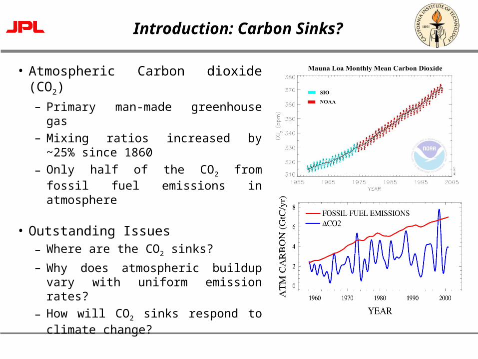
• Atmospheric Carbon dioxide (CO2)
– Primary man-made greenhouse gas
– Mixing ratios increased by ~25% since 1860
– Only half of the CO2 from fossil fuel emissions in atmosphere
• Outstanding Issues– Where are the CO2 sinks?
– Why does atmospheric buildup vary with uniform emission rates?
– How will CO2 sinks respond to climate change?

Page 4
Climate Change Discussions at the G8

Page 5
Why Measure CO2 from Space?
• Studies from GV-CO2 stations – Flux residuals exceed 1 GtC/yr in
some zones – Network is too sparse
• Inversion tests– Global XCO2 pseudo-data with 1
ppm accuracy – Flux errors reduced to < 0.5
GtC/yr/zone for all zones– Global flux error reduced by a
factor of ~3
Courtesy: Rayner and O’Brien, 2001
1.2
0.6
0.0
Flu
x Re
sidu
als (G
t/yr/zon
e)
1.2
0.6
0.0
Flu
x Re
sidu
als (G
t/yr/zon
e)
Page 6
Precise CO2 Measurements Needed
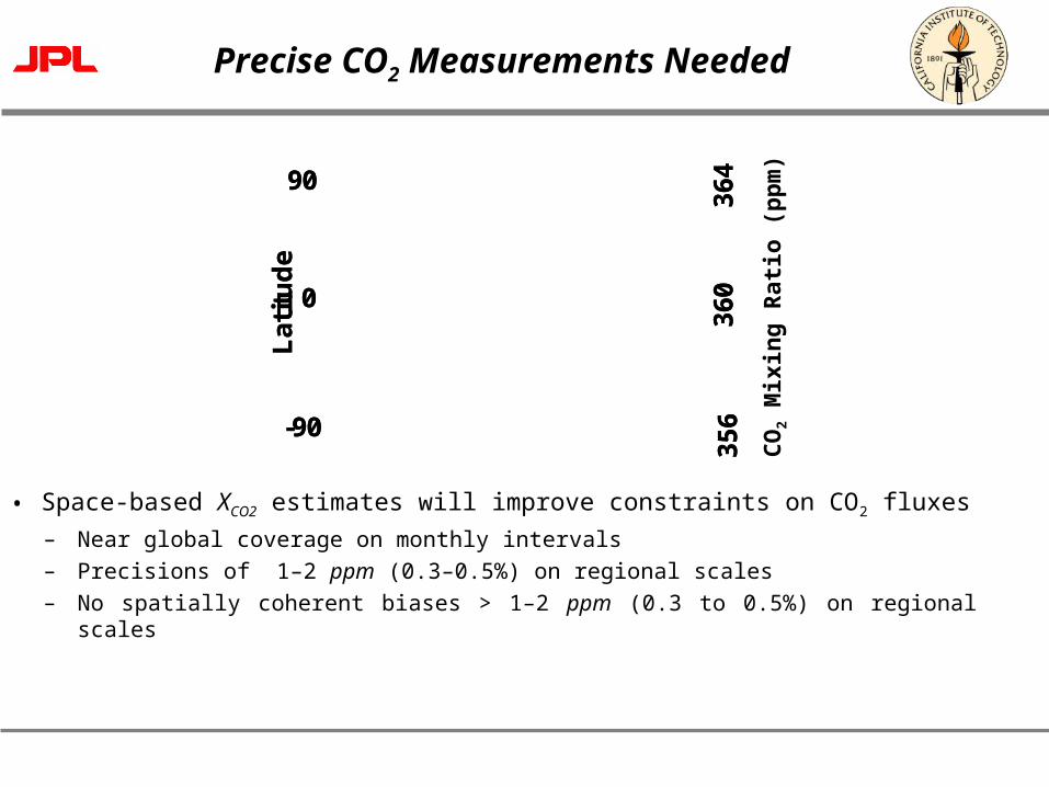
• Space-based XCO2 estimates will improve constraints on CO2 fluxes
– Near global coverage on monthly intervals
– Precisions of 1–2 ppm (0.3–0.5%) on regional scales
– No spatially coherent biases > 1–2 ppm (0.3 to 0.5%) on regional scales
CO
2 M
ixin
g R
atio
(p
pm
)
356
360
364
Lat
itu
de
90
-90
0
356
360
364
Lat
itu
de
90
-90
0
Page 7
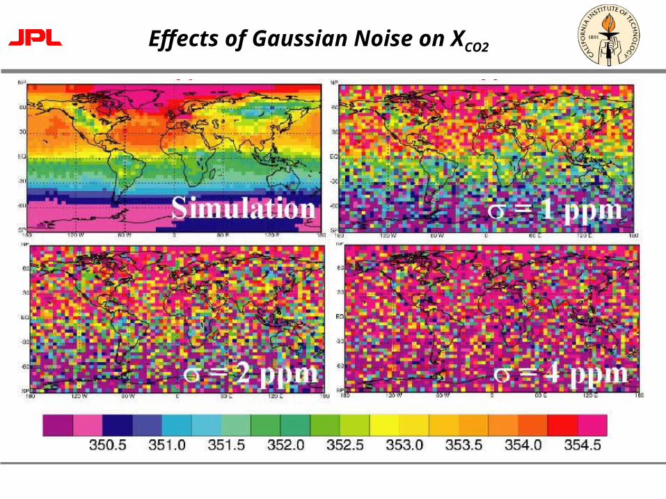
Effects of Gaussian Noise on XCO2
Page 8
The Orbiting Carbon Observatory (OCO)
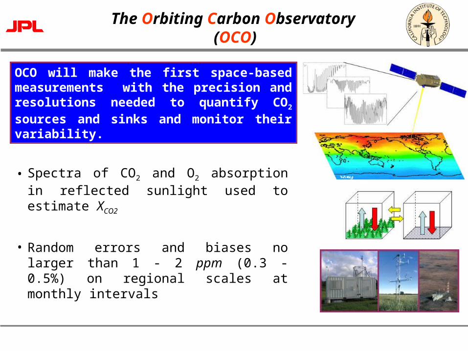
• Spectra of CO2 and O2 absorption in reflected sunlight used to estimate XCO2
• Random errors and biases no larger than 1 - 2 ppm (0.3 - 0.5%) on regional scales at monthly intervals
OCO will make the first space-based measurements with the precision and resolutions needed to quantify CO2 sources and sinks and monitor their variability.

Page 9
OCO Fills a Critical Measurement Gap
OCO will make precise global measurements of XCO2 needed to monitor CO2 fluxes on regional to continental scales.
Spatial Scale (km)
1
2
3
4
5
6
CO
2 E
rror
(pp
m)
1 10 100 1000 10000
OCO
FlaskSite
AquaAIRS
Aircraft
0
FluxTower
Globalview Network
NOAATOVS
ENVISATSCIAMACHY
Page 10
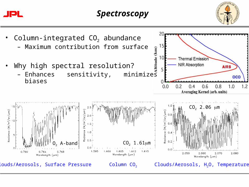
Spectroscopy
Clouds/Aerosols, Surface Pressure Clouds/Aerosols, H2O, TemperatureColumn CO2
O2 A-band CO2 1.61m
CO2 2.06 m
• Column-integrated CO2 abundance– Maximum contribution from surface
• Why high spectral resolution?– Enhances sensitivity, minimizes biases
Page 11
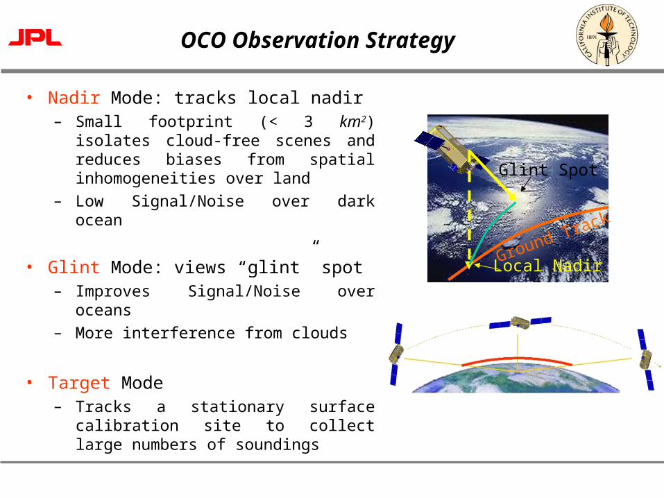
OCO Observation Strategy
• Nadir Mode: tracks local nadir– Small footprint (< 3 km2) isolates cloud-
free scenes and reduces biases from spatial inhomogeneities over land
– Low Signal/Noise over dark ocean
• Glint Mode: views “glint” spot– Improves Signal/Noise over oceans
– More interference from clouds
• Target Mode– Tracks a stationary surface calibration
site to collect large numbers of soundings
Local Nadir
Glint Spot
Ground Track

Page 12
OCO Retrieval Algorithm
Page 13
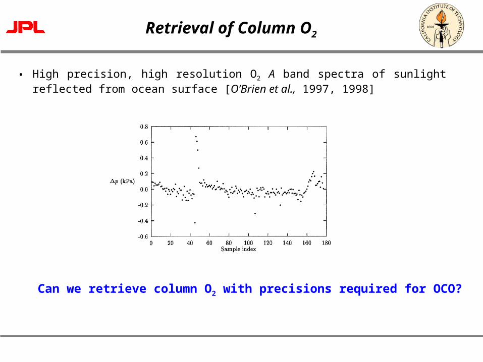
Retrieval of Column O2
• High precision, high resolution O2 A band spectra of sunlight reflected from ocean surface [O’Brien et al., 1997, 1998]
Can we retrieve column O2 with precisions required for OCO?

Page 14
Retrieval: First Cut
rms residual = 8.8%
Green - computed
Black - measured
Black - residual
Page 15
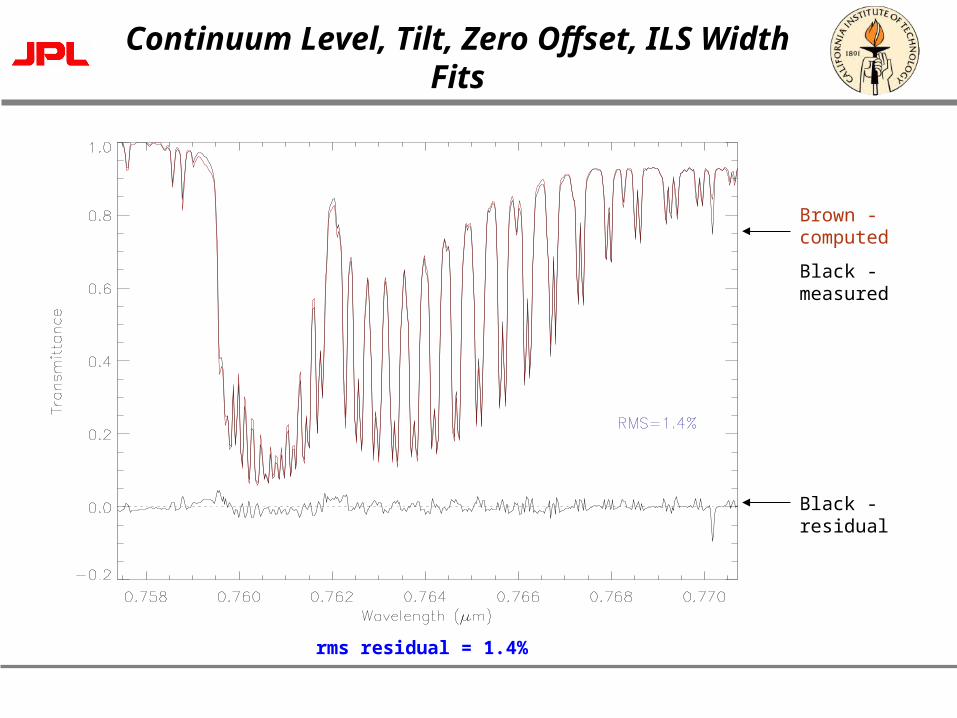
Continuum Level, Tilt, Zero Offset, ILS Width Fits
rms residual = 1.4%
Brown - computed
Black - measured
Black - residual

Page 16
Conclusions
• Algorithm developed to retrieve XCO2 from spectroscopic measurements of absorption in NIR bands
• Retrieved column O2 with precision ~ 1%
• Demonstrates potential to retrieve column O2 with precisions around 0.1% by averaging sufficient soundings
• Indicates feasibility of retrieving XCO2 with precisions better than 0.3%

Page 17
Aerosols: Major Source of Retrieval Uncertainty
Ground surface
Aerosol Layer 1
Aerosol Layer 2
Light reaching
the detector
Photon path length is modified
through multiple scattering by
aerosols
Incident light
Page 18
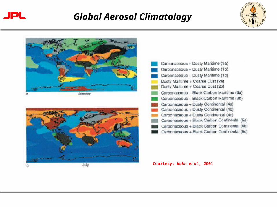
Global Aerosol Climatology
Courtesy: Kahn et al., 2001
Page 19
Aerosol Optical Properties
• Each mixing group is a combination of 4 different aerosol components from a basic set of 7 [Kahn et al., 2001].
• Sulfate (land/water), seasalt, carbonaceous, black carbon: spherical => Mie code [de Rooij and van der Stap, 1984]
• Mineral dust (accumulated/coarse): mixture of oblate and prolate spheroids => T-matrix code [Mishchenko and Travis, 1998]
• Lognormal distribution
• Polarization fully considered

Page 20
Scattering Matrix (755 nm)
Page 21
Forward Model Details
• Park Falls, Wisconsin, July (SZA = 31°)
• Exponential drop-off in aerosol extinction (scale height: ~ 1 km, optical depth: 0.1)
• Forward model: RADIANT [Christi and Stephens, 2004] + single scattering approximation for polarization
• Lorentzian instrument lineshape function (resolving powers: O2 A band: 17000, CO2 bands: 20000)
Page 22
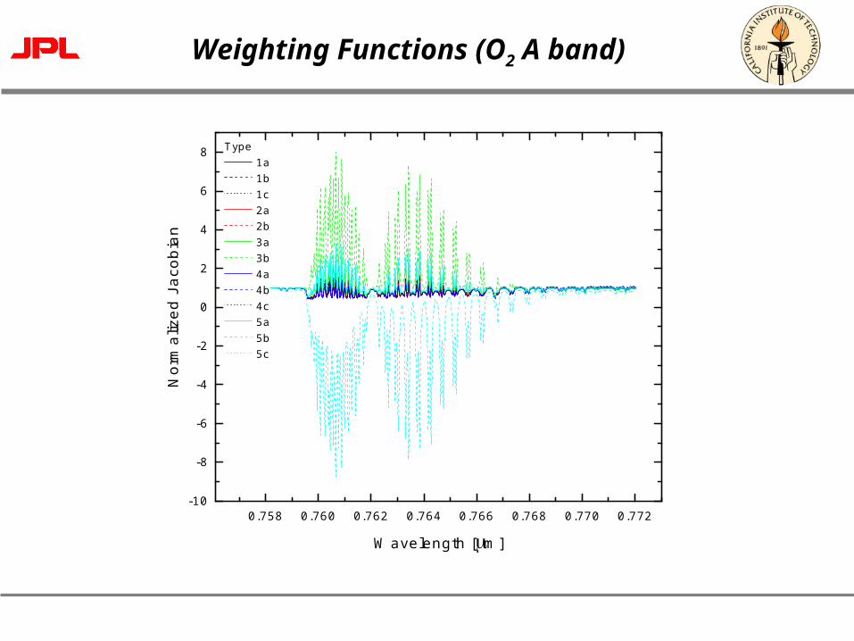
Weighting Functions (O2 A band)
0.758 0.760 0.762 0.764 0.766 0.768 0.770 0.772-10
-8
-6
-4
-2
0
2
4
6
8
Nor
mal
ized
Jac
obia
n
Wavelength [m]
Type 1a 1b 1c 2a 2b 3a 3b 4a 4b 4c 5a 5b 5c

Page 23
Weighting Functions (1.61 µm CO2 band)
1.590 1.595 1.600 1.605 1.610 1.615 1.620
-0.4
-0.2
0.0
0.2
0.4 Type 1a 1b 1c 2a 2b 3a 3b 4a 4b 4c 5a 5b 5c
Nor
mal
ized
Jac
obia
n
Wavelength [m]

Page 24
Weighting Functions (2.06 µm CO2 band)
2.04 2.05 2.06 2.07 2.08
-0.10
-0.05
0.00
0.05
0.10
No
rma
lize
d J
aco
bia
n
Type 1a 1b 1c 2a 2b 3a 3b 4a 4b 4c 5a 5b 5c
Wavelength [m]

Page 25
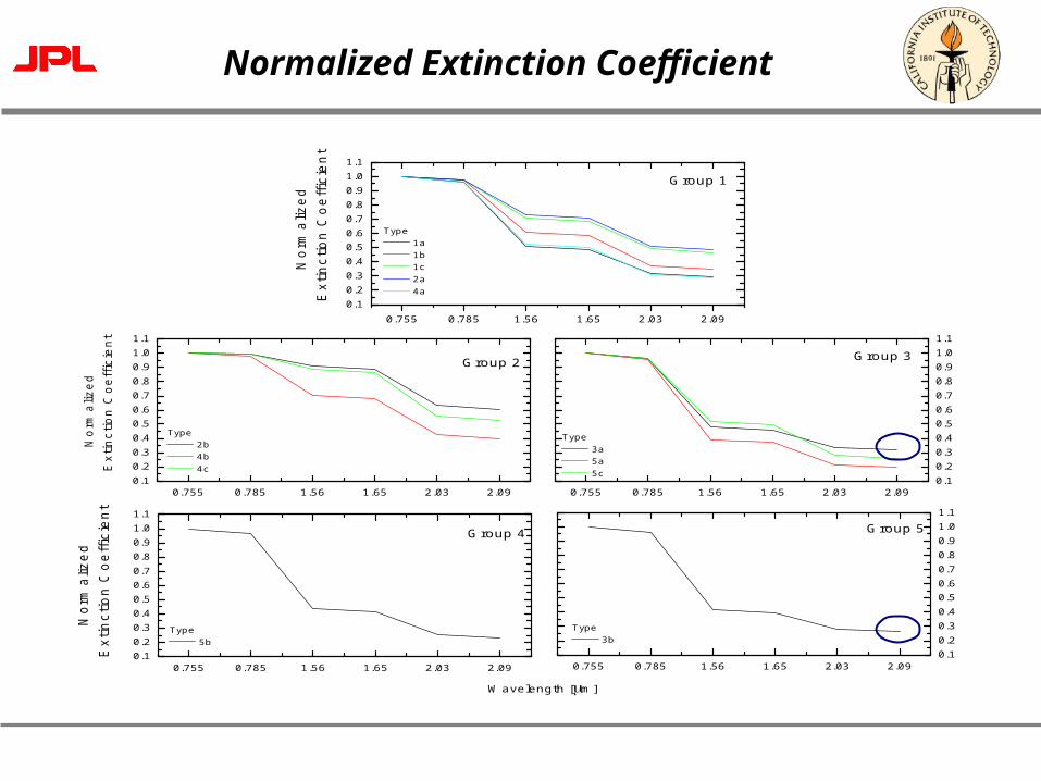
Normalized Extinction Coefficient
0.755 0.785 1.56 1.65 2.03 2.090.10.20.30.40.50.60.70.80.91.01.1
0.755 0.785 1.56 1.65 2.03 2.090.10.20.30.40.50.60.70.80.91.01.1
0.755 0.785 1.56 1.65 2.03 2.090.10.20.30.40.50.60.70.80.91.01.1
0.755 0.785 1.56 1.65 2.03 2.090.10.20.30.40.50.60.70.80.91.01.1
0.755 0.785 1.56 1.65 2.03 2.090.10.20.30.40.50.60.70.80.91.01.1
Norm
aliz
ed
Extinction C
oeffic
ient
Type 5b
Wavelength [m]
Group 4
Type 3b
Group 5
Type 2b 4b 4c
Norm
aliz
ed
Extinction C
oeff
icie
nt
Group 2
Type 3a 5a 5c
Group 3
Norm
aliz
ed
Extinction C
oeffic
ient
Type 1a 1b 1c 2a 4a
Group 1
Page 26
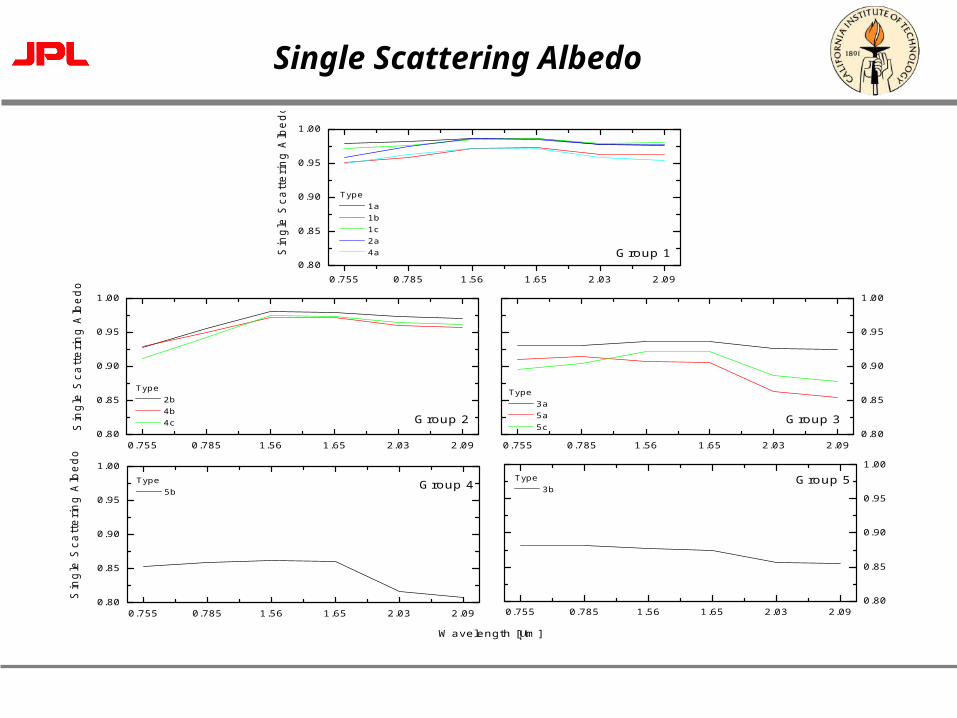
Single Scattering Albedo
0.755 0.785 1.56 1.65 2.03 2.090.80
0.85
0.90
0.95
1.00
0.755 0.785 1.56 1.65 2.03 2.090.80
0.85
0.90
0.95
1.00
0.755 0.785 1.56 1.65 2.03 2.090.80
0.85
0.90
0.95
1.00
0.755 0.785 1.56 1.65 2.03 2.090.80
0.85
0.90
0.95
1.00
0.755 0.785 1.56 1.65 2.03 2.090.80
0.85
0.90
0.95
1.00
Type 5b
Wavelength [m]
Sin
gle
Scatt
ering A
lbedo
Group 4Type
3b
Group 5
Type 2b 4b 4c
Sin
gle
Scatt
ering A
lbedo
Group 2
Type 3a 5a 5c
Group 3
Type 1a 1b 1c 2a 4a
Sin
gle
Scatt
ering A
lbedo
Group 1
Page 27
Normalized Extinction Coefficient
0.755 0.785 1.56 1.65 2.03 2.090.10.20.30.40.50.60.70.80.91.01.1
0.755 0.785 1.56 1.65 2.03 2.090.10.20.30.40.50.60.70.80.91.01.1
0.755 0.785 1.56 1.65 2.03 2.090.10.20.30.40.50.60.70.80.91.01.1
0.755 0.785 1.56 1.65 2.03 2.090.10.20.30.40.50.60.70.80.91.01.1
0.755 0.785 1.56 1.65 2.03 2.090.10.20.30.40.50.60.70.80.91.01.1
Norm
aliz
ed
Extinction C
oeffic
ient
Type 5b
Wavelength [m]
Group 4
Type 3b
Group 5
Type 2b 4b 4c
Norm
aliz
ed
Extinction C
oeff
icie
nt
Group 2
Type 3a 5a 5c
Group 3
Norm
aliz
ed
Extinction C
oeffic
ient
Type 1a 1b 1c 2a 4a
Group 1
Page 28
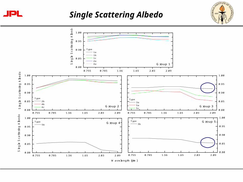
Single Scattering Albedo
0.755 0.785 1.56 1.65 2.03 2.090.80
0.85
0.90
0.95
1.00
0.755 0.785 1.56 1.65 2.03 2.090.80
0.85
0.90
0.95
1.00
0.755 0.785 1.56 1.65 2.03 2.090.80
0.85
0.90
0.95
1.00
0.755 0.785 1.56 1.65 2.03 2.090.80
0.85
0.90
0.95
1.00
0.755 0.785 1.56 1.65 2.03 2.090.80
0.85
0.90
0.95
1.00
Type 5b
Wavelength [m]
Sin
gle
Scatt
ering A
lbedo
Group 4Type
3b
Group 5
Type 2b 4b 4c
Sin
gle
Scatt
ering A
lbedo
Group 2
Type 3a 5a 5c
Group 3
Type 1a 1b 1c 2a 4a
Sin
gle
Scatt
ering A
lbedo
Group 1
Page 29
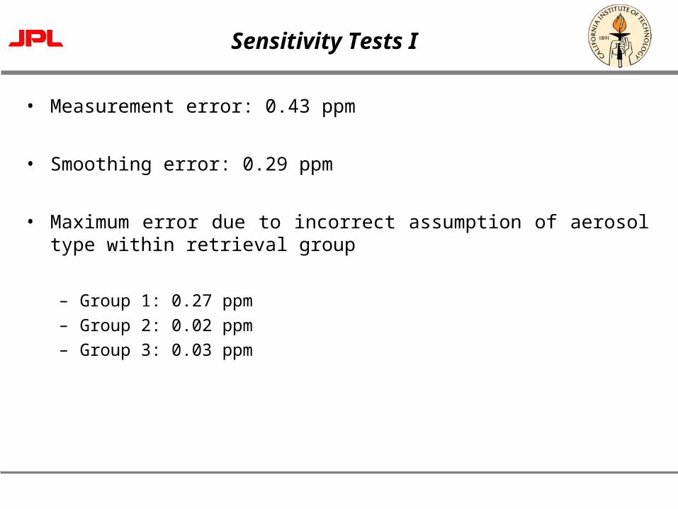
Sensitivity Tests I
• Measurement error: 0.43 ppm
• Smoothing error: 0.29 ppm
• Maximum error due to incorrect assumption of aerosol type within retrieval group
– Group 1: 0.27 ppm
– Group 2: 0.02 ppm
– Group 3: 0.03 ppm

Page 30
Sensitivity Tests II
Type 8 Type 9
1 2 3 4 5 6 7 8 9 10 11 12 130.00.20.40.60.81.01.21.41.6
Aerosol Type
1 2 3 4 5 6 7 8 9 10 11 12 130.00.20.40.60.81.01.21.41.6
Phase Matrix
Single Scattering Albedo
XC
O2 E
rror
(pp
m)
1 2 3 4 5 6 7 8 9 10 11 12 130.00.20.40.60.81.01.21.41.6 All Properties
1 2 3 4 5 6 7 8 9 10 11 12 130.00.10.20.30.40.50.60.70.8
Phase Matrix
Aerosol Type
1 2 3 4 5 6 7 8 9 10 11 12 130.00.10.20.30.40.50.60.70.8
Single Scattering Albedo
XC
O2
Err
or (
ppm
)
1 2 3 4 5 6 7 8 9 10 11 12 130.00.10.20.30.40.50.60.70.8
All Properties
Page 31
Conclusions
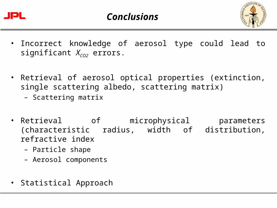
• Incorrect knowledge of aerosol type could lead to significant XCO2 errors.
• Retrieval of aerosol optical properties (extinction, single scattering albedo, scattering matrix)– Scattering matrix
• Retrieval of microphysical parameters (characteristic radius, width of distribution, refractive index– Particle shape
– Aerosol components
• Statistical Approach

Page 32
Polarization and the Stokes Parameters
• Electromagnetic radiation can be described in terms of the Stokes parameters: I, Q, U and V– I - total intensity
– Q & U - linear polarization
– V - circular polarization
• Degree of Polarization
(for OCO)I
Qp
I
VUQp
22
2
Page 33
Importance of Polarization
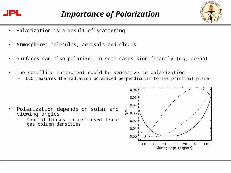
• Polarization is a result of scattering
• Atmosphere: molecules, aerosols and clouds
• Surfaces can also polarize, in some cases significantly (e.g., ocean)
• The satellite instrument could be sensitive to polarization– OCO measures the radiation polarized perpendicular to the principal plane
• Polarization depends on solar and viewing angles
– Spatial biases in retrieved trace gas column densities

Page 34
Two Orders of Scattering (2OS) to Compute Polarization
• Full multiple-scattering vector RT codes too slow to meet large-scale operational processing requirements
• Scalar computation causes two kinds of errors– Polarization components of the Stokes vector neglected
– Intensity incorrectly calculated
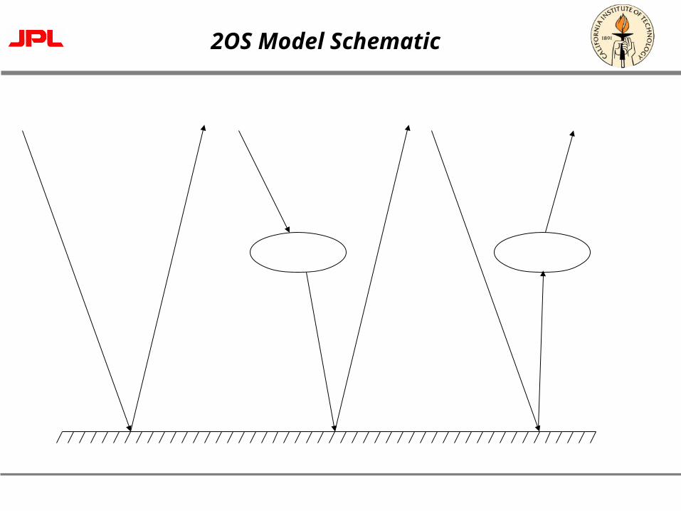
• Major contribution to polarization comes from first few orders of scattering (multiple scattering is depolarizing)
• Single scattering does not account for the correction to intensity due to polarization
Page 35
2OS Model Schematic
Page 36
2OS Model Outline
• Intensity still calculated with full multiple scattering scalar model
• S = Isca+Icor-Q2
• Fast correction to standard scalar code
• Exact through second order
• Analytic Jacobians
Page 37
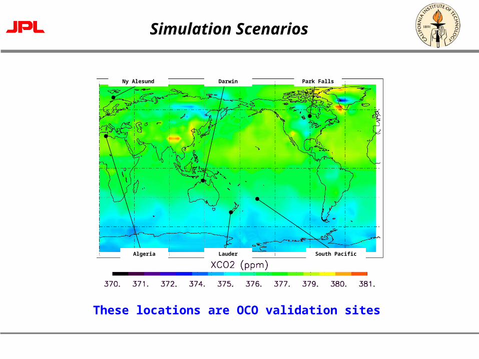
Simulation Scenarios
Darwin Park FallsNy Alesund
Algeria South PacificLauder
These locations are OCO validation sites
Page 38
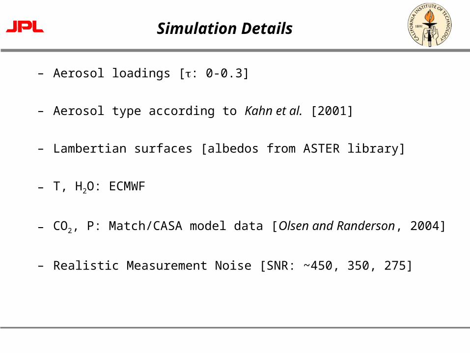
Simulation Details
– Aerosol loadings [: 0-0.3]
– Aerosol type according to Kahn et al. [2001]
– Lambertian surfaces [albedos from ASTER library]
– T, H2O: ECMWF
– CO2, P: Match/CASA model data [Olsen and Randerson, 2004]
– Realistic Measurement Noise [SNR: ~450, 350, 275]
Page 39
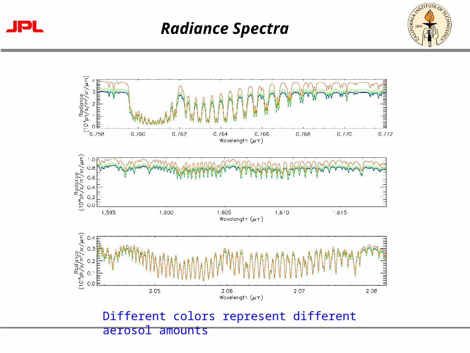
Radiance Spectra
Different colors represent different aerosol amounts
Page 40
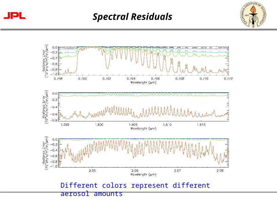
Spectral Residuals
Different colors represent different aerosol amounts

Page 41
Scalar Spectral Residuals
Different colors represent different aerosol amounts

Page 42
XCO2 and Surface Pressure Errors - I
Algeria (Jan)
Darwin (Jan)
Ny Alesund (Apr)
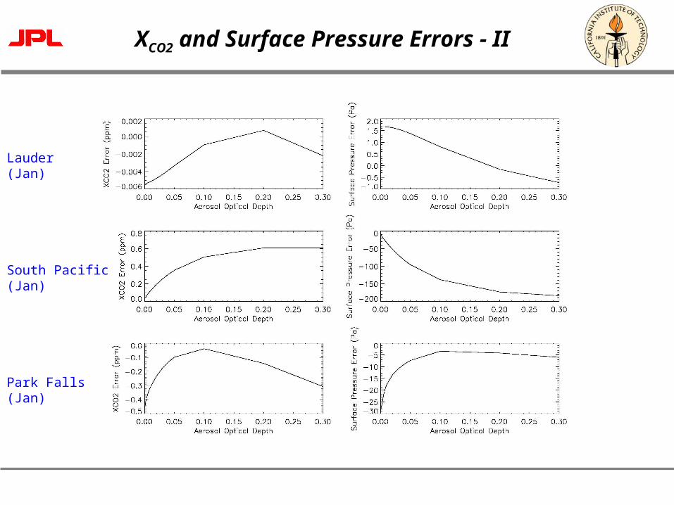
Page 43
XCO2 and Surface Pressure Errors - II
Lauder (Jan)
South Pacific (Jan)
Park Falls (Jan)

Page 44
XCO2 and Surface Pressure Errors - III
Algeria (Jan)
Darwin (Jan)
Ny Alesund (Apr)

Page 45
XCO2 and Surface Pressure Errors - IV
Lauder (Jan)
South Pacific (Jan)
Park Falls (Jan)

Page 46
Forward Model Error vs. Measurement Noise
2OS
Scalar

Page 47
Conclusions
• Ignoring polarization could lead to significant (~ 10 ppm) errors in XCO2 retrievals
• 2OS model gives XCO2 errors that are much smaller than other biases
• Two orders of magnitude faster than a full vector calculation
• Additional overhead in the range of 10% of the scalar computation
Page 48
Future Work
• Cirrus
• Surface Types
• Aerosol vertical distribution
• Spectroscopy
• Line Mixing
• Speed Improvements
Page 49
Acknowledgments
• Yuk Yung
• John Seinfeld, Rick Flagan, Paul Wennberg
• Hartmut Boesch, Rob Spurr
• David Crisp, Charles Miller, Geoff Toon, Bhaswar Sen, Hari Nair, James McDuffie, Denis O’Brien, Mick Christi
• Run-Lie Shia, Jack Margolis, Zhiming Kuang, Mao-Chang Liang, Xun Jiang, Dan Feldman, Xin Guo
• Friends
• Family

Page 50
To be continued …