Fizeau’s “aether-drag” experiment in the undergraduate laboratory

Thierry Lahaye,1, 2 Pierre Labastie,1, 2 and Renaud Mathevet1, 2, 3

1Universite de Toulouse, UPS, Laboratoire Collisions Agregats Reactivite, IRSAMC; F-31062 Toulouse, France2CNRS, UMR 5589, F-31062 Toulouse, France

3Laboratoire National des Champs Magntiques Intenses, UPR3228 CNRS/INSA/UJF/UPS, Toulouse, France(Dated: January 4, 2012)

We describe a simple realization of Fizeau’s “aether-drag” experiment. Using an inexpensive setup, wemeasure the phase shift induced by moving water in a laser interferometer and find good agreement with therelativistic prediction or, in the terms of 19th century physics, with Fresnel’s partial-drag theory. This appealingexperiment, particularly suited for an undergraduate laboratory project, not only allows a quantitative measure-ment of a relativistic effect on a macroscopic system, but also constitutes a practical application of importantconcepts of optics, data acquisition and processing, and fluid mechanics.

PACS numbers: 03.75.Kk,03.75.Lm

I. INTRODUCTION

In introductory courses and textbooks dealing with spe-cial relativity, Fizeau’s “aether-drag” experiment often ap-pears simply as an application of the law of composition ofvelocities, sometimes in the form of an exercise.1 However,Albert Einstein himself declared that Fizeau’s measurementof the speed of light in moving water was, together with stellaraberration, one of the experimental results that had influencedhim most in the development of relativity.2 In introductoryexpositions of Fizeau’s experiment, a discussion of the his-torical development of ideas that lead to it, as well as detailsabout the experimental setup itself, are often lacking. More-over, many textbooks actually show incorrect experimental ar-rangements that would not allow in practice for the observa-tion of the effect. Here we show that one can actually performFizeau’s experiment with rather modest equipment, and thatsuch a project illustrates in an appealing way not only rela-tivistic kinematics, but also interesting aspects of wave optics,data acquisition and processing, and even fluid mechanics.

This article is organized as follows. We first review brieflythe historical background of Fizeau’s experiment, a “test” ofspecial relativity carried out more than half a century beforerelativity was born! Then, for completeness, we recall inSection III the derivation of the expected fringe shift in boththe relativistic and non-relativistic frameworks, following theusual textbook treatment of the problem. We then turn to themain point of the paper, namely how to reproduce the exper-iment in an undergraduate laboratory. Section IV is devotedto the description of our apparatus, starting with an emphasison the experimental trade-offs one needs to address in the de-sign phase. Finally, we discuss in Sec. V the results obtained,first with water as a moving medium, and then with air, inorder to discriminate between relativistic and non-relativisticpredictions. The use of a white-light source instead of a laseris presented in appendix A, with a discussion of the possibleadvantages and drawbacks. Appendix B establishes a usefulfluid mechanics formula using dimensional analysis.

II. HISTORICAL BACKGROUND

Since Fizeau’s aether drag experiment is a landmark amongthe various experimental and theoretical developments lead-ing to special relativity, it is worthwhile to recall briefly thehistory of these developments. An extensive historical studyof the subject is beyond the scope of this paper: in whatfollows we merely recall the main steps that led to Fizeau’saether drag experiment, as well as the major subsequentdevelopments.3

We begin our reminder in the 17th century, at a time whenthe nature of light was a matter of harsh debate, as evidencedby the famous controversy between Christiaan Huygens andIsaac Newton. The measurement of the speed of light in amaterial medium of refractive index n was considered a cru-cial test since Huygens’ wave theory implies that the speed oflight in the medium is c/n, while Newton’s corpuscular theorypredicts it to be nc, where c is the speed of light in a vacuum,known to be finite since the work of Ole Romer in 1676.4

Newton’s views prevailed until the beginning of the 19th cen-tury, when interference experiments by Thomas Young andpolarization experiments by Etienne Malus firmly establishedthe wave theory.

An important step was the measurement by Francois Aragoof the deviation of light from a distant star by a prism in 1810.5

The idea of Arago is that if the speed of the light comingfrom distant stars is decreased or increased by the Earth ve-locity, Newton’s theory predicts that the deviation by a prismis different from what would be observed if the source wereterrestrial. He therefore tried to detect this difference, with anegative result. It seems to be the first experiment in a long se-ries, which showed the impossibility of detecting the relativemotion of light with respect to the Earth.6

Arago soon became friend with Augustin Fresnel, who hada mathematically sound theory of light waves, and asked himif the wave theory could explain the null result he had found.Fresnel’s answer came a few years later.7 His demonstrationis based on the hypothesis of an absolute aether as a supportof light waves, associated to a partial drag by transparent me-dia. That is, if the medium of index n moves with speed v,the aether inside the medium moves only at speed (1−n−2)v.

arX

iv:1

201.

0501

v1 [

phys

ics.

optic

s] 2

Jan

201

2

2

FIG. 1: (Color online) Sketch of the interferometer used by Fizeau.Figure adapted from.9 For the sake of clarity, the two counter-propagating beams are drawn in different colors. S: source; O: ob-server; M : mirror; Wi: windows; Li: lenses; BS: beam splitter;DS: double slit.

The value of Fresnel’s drag coefficient 1−n−2 precisely givesa null result for the Arago experiment. His demonstration, us-ing some supposed elastic properties of the aether, is howevernot so convincing by modern standards.6

The first Earth-based direct measurement of the speed oflight was realized in 1849, yet by Hippolyte Fizeau, by meansof a rotating cogwheel. This kind of time-of-flight techniquewas soon improved by Leon Foucault who, using a rotatingmirror, succeeded in showing that the speed of light is lower inwater than in air.8 Nevertheless, such absolute measurementswere far from accurate enough to measure the small change ofthe speed of light in moving media.

This is where Fizeau’s aether-drag experiment enters thescene. As we shall see, it is based on a much more sen-sitive differential measurement using the interferometric ar-rangement shown in Fig. 1. It was performed in 1851 andalmost immediately reported to the French academy of sci-ence, then translated in English.10 He measured an effect inagreement with Fresnel’s theory to within a few percent. Thisunambiguously ruled out concurrent theories postulating totalaether drag.

Many experiments of increasing precision were then under-taken to try to evidence the influence of Earth motion on lightpropagation, but all gave negative results. It soon became ap-parent that Fresnel’s partial drag prevented to measure any ab-solute motion of Earth to first order in v/c: in what would nowbe called a review paper,11 Eleuthere Mascart concludes in1874 (our translation): “the general conclusion of this mem-oir would be [...] that the translation motion of the Earth is ofno appreciable consequence on optical phenomena producedwith terrestrial sources or solar light, that those phenomena donot allow to appreciate the absolute motion of a body and thatonly relative motions can be attained.”

Then, in 1881 Albert Michelson designed a new interfer-ometer, which, according to existing theories, could evidenceEarth displacement respective to aether because the expectedeffect was proportional to (v/c)2. His first measurement wasat most half of the expected fringe shift. He then improvedthe apparatus with Edward Morley. The two physicists grad-ually became convinced of a negative result. In 1886 theydecided to redo Fizeau’s experiment, which was the only onewith a positive result, and had not been reproduced. With acareful design of the hydraulics part, and an improved designfor the interferometer,12 they were lead to confirm Fizeau’s

result, and Fresnel’s aether drag, with a much higher preci-sion. However, in their celebrated experiment of 188713 themeasured shift was at most 0.01 fringe instead of an expected0.4. The two experiments were thus incompatible accordingto existing theories, Fizeau’s one needing a partial drag andMichelson-Morley’s one a total drag of aether.

History then accelerated. In the late 1880’s, George Fitzger-ald proposed the length contraction. In 1895, HendrickLorentz published his theory of electromagnetic media, inwhich he derived Fresnel’s formula from first principles. Atthe beginning of the 20th century, it became evident thattime dilation was also necessary to account for all electro-magnetic phenomena. After Albert Einstein published thetheory of special relativity in 1905, Max Laue, in 1907, de-rived Fresnel drag coefficient from the relativistic addition ofvelocities.14 All experiments, being either of first (Fizeau) orsecond (Michelson-Morley) order in v/c, were then explainedby a single theory with no need for an aether with such specialproperties.

In the relativistic framework, one can also account for theeffects of dispersion, already predicted by Lorentz in 1895.Pieter Zeeman, in his 1914–27 experiments, tried to mea-sure this effect.15 The supplementary term makes only a fewpercent correction, but Zeeman succeeded in measuring it.16

More recently, the experiment was done in liquids, solids andgases using ring lasers17 and confirmed the value of the dis-persion term to within 15%.18 Fizeau’s experiment has alsobeen successfully transposed to neutron matter waves.19

As we have seen, Fizeau’s aether drag experiment was acrucial turning point between old and modern conceptions oflight and space-time. This therefore makes its replication par-ticulary valuable from a pedagogical point of view.

III. THEORETICAL BACKGROUND

In this section we recall the derivation of the phase differ-ence ∆ϕ induced by the motion, at velocity v, of the mediumof refractive index n in the interferometric arrangement shownin Fig. 2, which is essentially the one used by Michelson andMorley in 1886.12 Let us consider first the case where waterand monochromatic light, with vacuum wavelength λ, propa-gate in the same direction (shown in green on the figure). Inthe frame where water is at rest, the phase velocity of light isc/n. In the laboratory frame, using the relativistic composi-tion of velocities, the phase velocity of light is

v+ =c/n+ v

1 + (v · c/n)/c2=

c/n+ v

1 + v/(nc). (1)

The phase accumulated by light over the propagation distanceof 2` is thus

ϕ+ =2πc

λ

2`

v+. (2)

Where light and water propagate in opposite directions (redpath on the figure), the corresponding phase ϕ− is obtained by

3

FIG. 2: (Color online) Sketch of the experimental setup (see text fordetails). Mi: mirror; Wi: windows; BS: beam splitter. The twocounter-propagating beams are drawn in different colors for clarity.

replacing v by −v in the above result. The phase differencebetween the two arms of the interferometer thus reads:

∆ϕ = ϕ− − ϕ+ (3)

= 2π2`c

λ

(1− v/(nc)c/n− v

− 1 + v/(nc)

c/n+ v

). (4)

Expanding the above result to first order in v/c, we find:

∆ϕrel. = 2πv

c

4`

λ

(n2 − 1

). (5)

It is not difficult to do the same calculation using the non-relativistic addition of velocities v± = c/n ± v. One thenfinds:

∆ϕnon−rel. = 2πv

c

4`

λn2, (6)

i.e. the same functional form except for a coefficient n2 in-stead of n2 − 1. In Fresnel’s language, this would correspondto a complete aehter-drag. The ratio of the predictions (6) to(5) is about 2.3 for water (n = 1.33), and becomes very large(∼ 1700) for air (n − 1 = 3 × 10−4), whence the interestof performing the experiment also with air (see section V Ebelow).

As said before, the above derivation is first due to Laue in1907,14 and is the one found in most textbooks. It has beenpointed out16 that such an approach is not rigorous since therelativistic composition of velocities applies to point-like par-ticles, and not to the phase velocity of waves. However a rig-orous derivation, based on the Lorentz transformation of thefour-vector kµ = (ω/c,k) associated to light, gives the sameresult provided the light and the medium propagate along thesame axis.16

Up to now, we have neglected dispersion, i.e. the variationof the refractive index of the moving medium with the lightfrequency ω. However the frequency of the light in a movingframe is shifted by the Doppler effect. The shifts are oppo-site for the counterpropagating beams in the interferometer,

depicted in red and green in Figs. 1 and 2. They are then sub-jected to slightly different refraction indices due to dispersion.Then, in Eq. (5) the factor n2 − 1 has to be replaced by:20

n2 − 1 + nωdn

dω. (7)

Using the wavelength-dependent refractive index of waterfound in tables,21 a simple calculation shows that for waterat λ = 532 nm, the fringe shift is actually 3.8% greater thanwhat Eq. (5) predicts.

IV. EXPERIMENTAL SETUP: FIZEAU’S EXPERIMENTMADE EASY

A. Requirements

Fizeau’s experiment was a real tour de force made possibleby the very clever design of the experiment (Fig. 1). The im-provement by Michelson and Morley essentially transformsthe original wavefront-division setup into a much brighteramplitude-division one. In both arrangements, that we wouldcall now Sagnac interferometers,22 the two interfering beamsfollow almost exactly the same path (see Fig. 2). This not onlydoubles the interaction length with the moving medium, but,more importantly, rejects common-mode phase fluctuations(due e.g. to turbulence). This arrangement also ensures thatthe optical path length difference between the two interferingarms is zero when the interferometer is perfectly aligned (seesection V D below).

Equation (5) shows that the expected fringe shift is en-hanced by using a short wavelength λ, and a large product `v.Let us get an estimate of the requirements on the velocity. Wefirst set ` ∼ 2 m to make the size of the apparatus reasonable.Second we choose λ = 532 nm that corresponds to cheapdiode-pumped solid state lasers. Then one sees that achiev-ing a phase shift on the order of 1 rad with water (n ' 1.33)requires velocities on the order of 4 m/s. The experimentalsetup is thus required to allow for the detection of a shift ofa fraction of a fringe, and to produce a water flow of severalmeters per second.

The key in the success of the experiment is the care takenin doing the plumbing. We thus describe successively in moredetails the various components of our experimental setup andrefer the reader to the pictures shown in Fig. 3.

B. Hydraulics

For simplicity and low cost, we have built our system fromstandard piping material available in any hardware store, andin such a way that it can be fed from a regular tap. Ideallya large diameter d of the pipes is desirable. It simplifies thealignment of the interferometer beams and improves the ve-locity profile flatness over the beam section. However, thevolumetric flow rate reads Q = πd2v/4 and increases rapidlywith d. The typical maximal flow rates available at the wateroutlets of a laboratory are on the order of ten to twenty liters

4

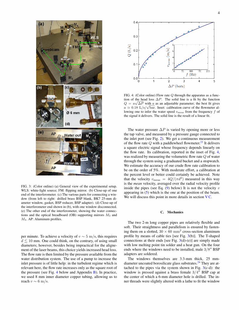
FIG. 3: (Color online) (a) General view of the experimental setup.WLS: white-light source; FM: flipping mirror. (b) Close-up of oneend of the interferometer. (c) The various parts for connecting a win-dow (from left to right: drilled brass BSP blank, BK7 25-mm di-ameter window, gasket, BSP reducer, BSP adapter). (d) Close-up ofthe interferometer end shown in (b), with one window disconnected.(e) The other end of the interferometer, showing the water connec-tions and the optical breadboard (OB) supporting mirrors M3 andM4. AP: Aluminum profiles.

per minute. To achieve a velocity of v ∼ 5 m/s, this requiresd . 10 mm. One could think, on the contrary, of using smalldiameters; however, besides being impractical for the aligne-ment of the laser beams, this choice yields increased head loss.The flow rate is then limited by the pressure available from thewater distribution system. The use of a pump to increase theinlet pressure is of little help: in the turbulent regime which isrelevant here, the flow rate increases only as the square root ofthe pressure (see Fig. 4 below and Appendix B). In practice,we used 8 mm inner diameter copper tubing, allowing us toreach v ∼ 6 m/s.

FIG. 4: (Color online) Flow rate Q through the apparatus as a func-tion of the head loss ∆P . The solid line is a fit by the functionQ = a

√∆P with a as an adjustable parameter; the best fit gives

a ' 0.18 L/s/√

bar. Inset: calibration curve of the flowmeter al-lowing one to infer the water speed vmeas from the frequency f ofthe signal it delivers. The solid line is the result of a linear fit.

The water pressure ∆P is varied by opening more or lessthe tap valve, and measured by a pressure gauge connected tothe inlet port (see Fig. 2). We get a continuous measurementof the flow rate Q with a paddlewheel flowmeter.23 It deliversa square electric signal whose frequency depends linearly onthe flow rate. Its calibration, reported in the inset of Fig. 4,was realized by measuring the volumetric flow rateQ of waterthrough the system using a graduated bucket and a stopwatch.We estimate the accuracy of our crude flow rate calibration tobe on the order of 5%. With moderate effort, a calibration atthe percent level or better could certainly be achieved. Notethat the velocity vmeas = 4Q/(πd2) measured in this wayis the mean velocity, averaged over the radial velocity profileinside the pipes (see Eq. (9) below) It is not the velocity vappearing in (5) which is the one at the position of the beam.We will discuss this point in more details in section V C.

C. Mechanics

The two 2-m long copper pipes are relatively flexible andsoft. Their straightness and parallelism is ensured by fasten-ing them on a slotted, 30 × 60 mm2 cross-section aluminumprofile by means of cable ties [see Fig. 3(b)]. The T-shapedconnections at their ends [see Fig. 3(d)-(e)] are simply madewith low melting point tin solder and a heat gun. On the fourends where the windows need to be installed, male 3/8′′ BSPadapters are soldered.

The windows themselves are 3.3-mm thick, 25 mm-diameter uncoated borosilicate glass substrates.24 They are at-tached to the pipes via the system shown in Fig. 3(c-d): thewindow is pressed against a brass female 3/4′′ BSP cap atthe center of which a 6-mm diameter hole is drilled. The in-ner threads were slightly altered with a lathe to fit the window

5

outer diameter. The cap and window are then tightened witha fiber gasket onto a male-male BSP 3/4′′ to 3/8′′ adapterwhich is itself connected to the male BSP adapter soldered tothe pipe via a female-female 3/8′′ BSP adapter.

The one end with hoses connected to the water inlet andoutlet in the laboratory sink is extending over the side ofthe table (see Fig. 3(e)). Two L-shaped aluminum profilesscrewed on the table support a small piece of optical bread-board on which we mount the two mirrors M3 and M4. Ina preliminary set of experiments we tried a configuration inwhich the water pipes were supported independently fromthe optical table (and thus from the interferometer) in or-der to avoid possible detrimental vibrations. However, thiswas somehow cumbersome, and the much simpler solution ofclamping tightly the pipes to the optical table (by means offour regularly spaced post-holders) does not yield any degra-dation of the measurements.

D. Optics and alignement

As a light source, we use a cheap diode-pumped, solid state(DPSS) laser delivering a quasi-collimated beam with severalmilliwatts of light at λ = 532 nm.25 The metallic mirrors M0

to M4 and the dielectric beamsplitter are all mounted on kine-matic optical mounts. We found it convenient to draw directlythe light path on the optical table (see Fig. 3(b)) before pre-cisely mounting the mirrors and the beamsplitter on the op-tical table. This considerably simplifies the alignment of theinterferometer, which is done in the following way.

First, four small diaphragms (diameter ∼ 2 mm) are po-sitioned just in front of the centers of the windows W1−4.The tubing system is then removed, and one walks the beamusing the controls of M1, BS and M2 in order to have thebeams W1W4 and W2W3 passing through the diaphragms.Then, using M3 and/or M4, one aligns the returning beamsonto the ingoing ones. In this way, one obtains (possibly aftersome iterations) a quasi-perfect superposition of the beams,and observes an almost flat intensity profile in the interfer-ence field. When tilting slightly one of the mirrors (e.g., M3),nice straight parallel fringes appear.

Now the pipes can be positioned back and clamped ontothe table. Water is set to flow, and one makes sure that no airbubble is trapped inside the pipes, especially close to the win-dows where the diameter is larger. If so, they can be removedby unfastening a little bit the cap while water is flowing.

Instead of the expected fringe pattern, one usually observescaustics and diffuse reflections on the inner sides of the pipes.Indeed, due to the soldering, the parallelism of the windowscannot be ensured. When a beam strikes the window at a smallangle from the normal, it is slightly deviated. This deviationis here only partially compensated at the inner glass/water in-terface. The interferometer has thus to be realigned. After afew iterations, fringes are back (see Fig. 5).

FIG. 5: (Color online) Sample images of the fringe pattern obtainedon the camera for (a) v = −5.7 m/s, (b) v = 0.8 m/s, and (c)v = 5.7 m/s. The white dashed line shows the position x0 of thecentral fringe for v = 0. (d) Processing of the image shown in (c):the dots are the vertically integrated intensity, and the (red) solid linethe best fit to (8).

V. EXPERIMENTAL RESULTS

A. Data acquisition

For quantitative measurements of the fringe shift, we usean inexpensive webcam26 whose objective lens and IR filterhave been removed, in order to expose directly the CMOS de-tector chip to the fringe pattern. Using the micrometer screwsof mirror M2 for instance the fringes are set parallel to oneof the axes of the camera chip. From the webcam softwarethe gamma correction is set to zero to get a linear responseof the detector.27 The integration time and light intensity areadjusted to use the full dynamic range of the webcam, takingcare not to saturate any pixel.

An important point for later data processing is that, prior toacquiring a series of images, one needs to locate the positionof the central fringe on the camera. For this, it is convenientto wobble mirror M2 for example. The fringe spacing varies,and the fringes move symmetrically away from the central onewhich is dark and does not move. Once the position x0 ofthe central fringe has been located, the webcam is roughlycentered on it, to limit systematic errors due to changes in thefringe spacing (see section V D). The fringe spacing is thenadjusted to get about ten fringes on the detector chip. Too fewfringes would not allow for an accurate measurement of thefringe position offset and period. On the other hand, if thefringes are too narrow, the resolution of the camera will limitaccuracy.

6

FIG. 6: (Color online) Experimental results for water as a movingmedium. Circles: data; thin solid line: linear fit, giving a slope of0.274 ± 0.003 rad s/m; thick solid line: relativistic theoretical ex-pression (5); dashed line: non-relativistic theoretical expression (6).

B. Data processing

We process the images in the following way. We sum upthe values of all pixels in a column, and thus obtain a one-dimensional intensity distribution I(x), where x (in pixels)denotes the position along an axis perpendicular to the fringes(Figure 5). We then fit the data I(x) by the following func-tional form

I(x) = I0 + I1 sin

(2π(x− x0)

Λ+ ∆ϕ

). (8)

Here, I0, I1, Λ and ∆ϕ are adjustable parameters, and x0 isthe (fixed) position of the central fringe, determined as ex-plained above.

C. Experimental results with water

Acquisition and processing is repeated for various water ve-locities. Figure 6 shows the experimentally measured phasedifference ∆ϕ as a function of the water velocity v. Theorigin of phases has been chosen to vanish at zero velocity.As can be seen on the figure, we take five measurements foreach velocity in order to increase statistics and get an esti-mate of the dispersion of the results. Negative velocities wereobtained simply by exchanging the inlet and outlet ports ofthe tubing system. No points could be recorded for veloci-ties below 1 m/s. Indeed, when the velocity is low, turbu-lence in the pipes is not fully developed which leads to lowspatial and temporal frequency fluctuations and very unstablepictures. We could not measure the point at zero velocity ei-ther, as for this measurement the inlet or outlet valve has tobe closed. This produces too few or too much effort on thetubing system which is not stiff enough and light does not getout properly any more. That is why the alignement procedurehas to be done, once and for all, but with water flowing in thepipes.

FIG. 7: (Color online) Dashed line: Poiseuille’s velocity profilefor laminar flow: v(r) = vmax(1 − r2/R2). Solid line: veloc-ity profile for turbulent flow, modeled here by the empirical formv(r) = vmax(1− r2/R2)1/6.

We observe a clear linear dependence of ∆ϕ on vmeas.A linear fit (shown as the thin solid line) gives a slope of0.274±0.003 rad s/m. The dashed line is the non-relativisticprediction (6), with slope 0.563 rad s/m which does notmatch at all the experimental results. The relativistic predic-tion (5), shown as the thick solid line (slope 0.248 rad s/m),is in much better agreement with the experimental data. How-ever, we observe that the experimental points almost system-atically lie above the predicted value. This comes from thefact that, as said earlier, we measure the mean velocity vmeas

averaged over the velocity profile inside the pipes, whereaswe need the velocity v appearing in (5) which is the one at theposition of the beam, i.e. on the pipes’ axis.

Let v(r) denote the radial dependence of the velocity in thepipes of radius R and vmax = v(0). As, by construction, thebeam is well centered on the pipe one can safely assume v =vmax. We must therefore multiply the theoretical predictionby the following correction factor

vmax

vmeas= πR2vmax

/∫ R

0

2πrv(r) dr . (9)

A theoretical model for the radial dependence v(r) is thus re-quired. In the laminar regime (Poiseuille flow), v(r) wouldhave the parabolic shape shown as a dashed line in Fig. 7, andthe correction factor (9) would be equal to 2. But one cancheck that, for v & 1 m/s, the Reynolds number Re = vd/νis already on the order of Re & 104 and the flow is turbu-lent. In the above expression ν ∼ 10−6 m2/s denotes thekinematic viscosity of water. Under these conditions, there isno simple rigorous analytical expression for the velocity pro-file. However, for the range of Reynolds numbers used here,experimentally measured flow profiles are well reproduced bythe empirical law v(r) = vmax(1− r2/R2)1/6,12 correspond-ing to a much flatter velocity profile (see Fig. 7). Equation (9)then gives a correction factor of 1.16. The relativistic pre-diction (5) multiplied by this correction factor, and including

7

also the 3.8% correction due to dispersion, yields a slope of0.299 rad s/m (not shown on Fig. 6). The agreement be-tween the experimental and theoretical values is thus at thelevel of 8%.

D. Discussion

First of all, we conclude that the non-relativistic predictionis clearly ruled out by our measurements. However, the rathergood agreement with the relativistic prediction must not beover interpreted. Indeed it is difficult to put a very accurateerror bar on the result, as several systematic effects should bestudied carefully for such a purpose. First, as stated above, thesystematic errors are dominated by our flowrate measurement.A more careful calibration should thus be performed in orderto improve the accuracy. Then, the factor of about 1.16 dueto the shape of the velocity profile should be measured forour system. A final source of uncertainty is the determinationof the actual length ` appearing in (5). In practice, the flowmakes a right-angle turn at each end of the pipes. The velocitydistribution is affected up and downstream on length scalespresumably on the order of the pipe diameter d. This impliesa correction of order d/` (i.e., on the percent level) but, again,an accurate estimation is difficult.

In the end, due to slight distortion of the the tubing whenthe velocity, and thus the pressure, is varied, the fringe spacingchanges a little bit. As said above, an important feature ofthe Sagnac-like interferometric arrangement used here is that,by construction, it operates at low interference order p. Thisis crucial in order to be sure that when the water is flowinginside the pipes, the observed shift of the fringes does arisefrom the aether drag effect and not from a slight change inthe fringe spacing. As an example, let us assume that usinga different interferometric setup, one observes an interferencepattern with 10 fringes, corresponding to interference orders,say p1 = 104 to p2 = p1 + 10. If, as is very likely, the fringespacing changes by a quantity as small as 10−4 in relativevalue when the water velocity varies, one would observe thatour ten fringes would shift, almost as a whole, by as much asone full fringe! We have measured that, for the data presentedin the paper, the fringe period Λ does not vary by more than5% over the full range of velocities, yielding negligible errorsdue to the low interference orders used here.

E. Experimental results with air

In his original paper,10 Fizeau states that he performed theexperiment with air as a moving medium and that (our trans-lation) “the motion of the air does not produce any sensibledisplacement of the fringes”, in agreement with the partialdrag prediction (5). On the contrary, the non-relativistic equa-tion (6) predicts a measurable shift.

It is thus interesting to perform the experiment also with air.We do so by using a standard compressed air outlet, as avail-able in most laboratories. One actually needs very moderatepressures in order to achieve relatively high velocities for the

FIG. 8: (Color online) Experimental results for air as a movingmedium. Circles: data; solid line: relativistic prediction (5); dashedline: non-relativistic prediction (6).

air flow in the d = 8 mm pipes: only 0.2 bar typically yieldsvmeas ' 35 m/s. Measuring the air velocity is not as straight-forward as with water; we found it convenient to use a hot-wire anemometer28 placed in a D = 18 mm inner diameterpipe at the outlet of the d = 8 mm pipes. The velocity vmeas

in the interaction region of the interferometer is then deducedfrom the measured velocity vanem at the anemometer positionvia volumetric flow conservation vmeas = vanem(D/d)2. Thisassumes incompressible flow, which is valid since the air ve-locity is much smaller here than the speed of sound.29

Figure 8 shows the measured phase shifts (circles) alongwith the predictions of equation (5) and (6). We could notclearly identify the reason(s) behind the seemingly oscillatingbehavior of the measured fringe shift with velocity. In anycase, the non-relativistic prediction is clearly ruled out by themeasurements, which are, on the contrary, compatible withthe relativistic calculation.

VI. CONCLUSION AND OUTLOOK

Using rather modest equipment, we have shown thatFizeau’s “aether-drag” experiment can be reproduced in theundergraduate laboratory at a quantitative level. It not onlymakes a nice practical introduction to the sometimes abstractconcepts of special relativity, but also constitutes an interest-ing application of several branches of experimental physics.

Immediate improvements of the setup described in this pa-per would consist in (i) calibrating the flowrate more carefully,and (ii) increasing the stiffness of the tubing system. A nat-ural extension of this work, suitable for a long-term studentproject, would consist in trying to study in details systematiceffects, for instance the determination of the effective length`. A possible way to measure this systematic effect could beto start from the full pipe length and then repeat the experi-ment for shorter and shorter pipe lengths. The effect can thenbe evaluated measuring the dependence of the slope ∆ϕ/v onthe pipe length.

8

FIG. 9: (Color online) (a) A sample white-light fringe pattern. (b)Composite image of 22 fringe patterns obtained for different watervelocities v. One clearly observes the linear shift of the central fringeposition as a function of v.

A more ambitious extension, suitable for advanced under-graduates, would illustrate more modern optical techniques.For instance, one may use a ring cavity of moderately high fi-nesse (say F ∼ 100 to 1000) and measure the variation of theresonance frequencies of the two counterpropagating modeswhen the velocity of the medium is varied. A gain in sensi-tivity by a factor F is then expected. Such techniques, withultra-high finesse cavities, are currently used to measure e.g.non-reciprocity effects in the propagation of light with amaz-ing sensitivities.30

Acknowledgments

We thank Eric Desmeules for being at the origin ofthis work and his students Melodie Andrieu and LauraneBoulanger for help in setting up a preliminary version ofthe apparatus during their ‘TIPE’ project: the data shown inFigs. 4 and 6 were essentially acquired by them. We thankJacques Vigue for useful discussions. David Guery-Odelincreated the conditions that made this project possible. R. M.dedicates his contribution to Jose-Philippe Perez for inspiringdiscussions over the years. Funding by CNRS is acknowl-edged.

Appendix A: Using a white-light source instead of a laser

We have also performed the experiment using a white-lightsource instead of a laser. The source is a 1-mm diameter irisilluminated by a 55 W halogen lamp (of the type used forcar headlights) and a condenser lens. The resulting divergingbeam is collimated by a 100-mm focal length lens, and super-imposed onto the path of the laser beam using two mirrors.The second one, located between M0 and M1, is a flippingone so that one can switch easily between the laser and thewhite light source (see Fig. 3(a)). Once the interferometerhas been aligned with the laser, white-light fringes are read-ily observed. Naturally, if the iris is opened the luminosity isincreased at the expense of spatial coherence. The contrast ofpicture is lost. The fringes are then localized in the vicinityof mirror M3. A colorful image as Fig. 9(a) is then recovered

with a converging lens that conjugates M3 and the detectorplane.

The advantages of using a white source is that (i) the po-sition of the dark central fringe can be found without ambi-guity as the contrast of the colored fringes vanishes rapidlyaway from the zero path-length difference, and (ii) as com-pared to using a laser is that unwanted interference fringes,due to scattering on dust particles for instance, as well asspeckle, are suppressed. There are however a certain num-ber of drawbacks. Besides the reduced luminosity, makingquantitative comparisons with theory is obviously much moredifficult than in the monochromatic case. Indeed, one wouldneed to measure the light spectrum, as well as the wavelength-dependent reflectivity (including phaseshifts) introduced bythe beamsplitter in order to model quantitatively the fringepattern. For instance, we have observed indeed that using ametallic beamsplitter instead of a the dielectric one alters sig-nificantly the colors and the contrast of fringe pattern obtainedin white light.

We made a composite of 22 images taken for various watervelocities v. The result, shown on Fig. 9(b)), clearly showsthat the fringe position shift linearly with velocity. However,as explained above, a quantitative analysis of such an imageis not easy, and the motivation behind this figure is more of anesthetic character.

Appendix B: Turbulent head loss in a circular pipe: dimensionalanalysis approach

In the standard introductory physics curriculum, the com-putation of the head loss in a circular pipe is done usingPoiseuille’s equation, valid for laminar flow. It is much lessfrequent to present te case of turbulent flow to undergradu-ate students. Reference to the Moody diagram giving the so-called friction factor as a function of the Reynolds number(and pipe roughness) can be found in engineering-orientedtextbooks, but may appear as quite involved to beginningphysics students. In this small appendix, we show how simpledimensional analysis can be used to infer a plausible expres-sion for the turbulent head loss, at least its dependence on flowrate and pipe diameter, two parameters that are crucial for thedesign of our experimental setup.

We consider the head loss ∆P for the flow of a fluid ofdensity ρ and kinematic viscosity ν across a circular pipe ofdiameter d and length l, flowing with a volumetric flow rateQ. Let us make two assumptions. First, for an infinitely longpipe, only the pressure gradient ∆P/l is physically relevant.Moreover, the limit of a very large Reynolds number corre-sponds formally to the limit ν → 0. Then, in that case, theviscosity ν should not appear explicitly in the expression forthe head loss. Under these conditions, we expect the followingfunctional form for the head loss to hold:

∆P

l= AραQβDγ , (B1)

where A is a dimensionless constant and (α, β, γ) exponentsto be determined. Equating the dimensions of both sides of

9

the above equation yields three equations for the exponents,giving in the end:

∆P

l= A

ρQ2

D5. (B2)

This expression agrees well with empirical formulae used in

an engineering context if one chooses A ∼ 3 × 10−2. Thisis typically what one would find using the friction factor ob-tained in Moody diagram31,32 for our typical Reynolds num-bers. The value of the coefficient a obtained in fitting theQ(∆P ) data of Fig. 4 yields A ' 2.5× 10−2, in good agree-ment with the previous estimate.

1 E. F. Taylor and J. A. Wheeler, Spacetime Physics: Introductionto Special Relativity 2nd edition (W. H. Freeman & Company),1992.

2 R. S. Shankland, “Conversations with Albert Einstein,” Am. J.Phys. 31, 47–57 (1963).

3 For a detailed account, see: O. Darrigol, “The genesis of theTheory of Relativity,” Seminaire Poincare 1, 1–22 (2005), avail-able online at <www.bourbaphy.fr/darrigol2.pdf>, and refer-ences therein.

4 O. Romer, “Demonstration touchant le mouvement de la lumieretrouve par M. Romer de l’Academie Royale des Sciences,” Jour-nal des Scavans, 233–236 (1676). An English translation appearedquickly in Phil. Trans. 12, 893–894 (1677), available online at<http://dx.doi.org/10.1098/rstl.1677.0024>.

5 He gave an account of the results to the French Academyof Sciences, but the text was not published until 1853in F. Arago, “Memoire sur la vitesse de la lumiere,”C. Rend. Ac. Sci. 36, 38–49 (1853). Available online at<http://gallica.bnf.fr/ark:/12148/bpt6k2993z/f42.image>.

6 For a modern account see R. Ferraro and D. M. Sforza, “Arago(1810): the first experimental result against the ether,” Eur. J.Phys. 26, 195–204 (2005).

7 A. Fresnel, “Lettre de M. Fresnel a M. Arago, sur l’influencedu mouvement terrestre dans quelques phenomenes d’optique,”Ann. Chim. Phys. 9, 57–66 (1818). Available online at<http://www.google.com/books?id=nZc5AAAAcAAJ>.

8 L. Foucault, Sur les vitesses relatives de la lumiere dansl’air et dans l’eau (Bachelier, Paris) 1853. Available online at<http://www.bibnum.education.fr/files/foucault-texte.pdf>.

9 A. A. Michelson, Studies in Optics (Dover, New-York) 1995.10 H. Fizeau, “Sur les hypotheses relatives a l’ether lumineux, et sur

une experience qui paraıt demontrer que le mouvement des corpschange la vitesse avec laquelle la lumiere se propage dans leurinterieur,” C. R. Acad. Sci. 33, 349–355 (1851); translated intoEnglish in H. Fizeau, “On the effect of the motion of a body uponthe velocity with which it is traversed by light” Phil. Mag. 4th

series 2, 568–571 (1851). A longer account, with the same title,was published in H. Fizeau, Ann. Chim. Phys. 57, 385–404 (1859)and translated in H. Fizeau, Phil. Mag. 4th series 19, 245–260(1860).

11 E. Mascart, “Sur les modifications qu’eprouve la lumiere parsuite du mouvement de la source lumineuse et du mouvement del’observateur,” Ann. Sci. Ec. Norm. Sup. 2nd series 3, 363–420(1874). Available online at <http://www.numdam.org/numdam-bin/feuilleter?j=asens>.

12 A. A. Michelson and E. W. Morley, “Influence of Motion ofthe Medium on the Velocity of Light,” Am. J. Sci. 31, 377–386(1886).

13 A. A. Michelson, W. Morley, “On the relative motion of the Earthand the luminiferous ether,” Am. J. Sci. 34, 333–345 (1887).

14 M. Laue, “Die Mitfuhrung des Lichtes durch bewegte Korper

nach dem Relativitatsprinzip,” Ann. Phys. 328, 989-990 (1907).15 P. Zeeman, “Fresnel’s coefficient for light of different colours

(first part),” Proc. Roy. Acad. Amsterdam 17, 445–451 (1914);“Fresnel’s coefficient for light of different colours (secondpart),”ibid. 18, 398–408 (1915).

16 However, this experiment was recently revisited by Lerche whoclaims, on the basis of ignored systematic effects, that Zeeman’sexperiments are inconclusive. See I. Lerche, “The Fizeau effect:Theory, experiment, and Zeeman’s measurements,” Am. J. Phys.45 1154–1164 (1977).

17 W. M. Macek, J. R. Schneider and R. M. Salamon, “Measurementof Fresnel Drag with the Ring Laser,” J. Appl. Phys. 35, 2556–2557 (1964).

18 H. R. Bilger and A. T. Zavodny, “Fresnel Drag in a Ring Laser:Measurement of the Dispersive Term,” Phys. Rev. A 5, 591–599(1972).

19 A. Klein et al., “Neutron Propagation in Moving Matter: TheFizeau Experiment with Massive Particles,” Phys. Rev. Lett. 46,1551–1554 (1981).

20 J. D. Jackson, Classical Electrodynamics, 3rd edition (Wiley,New-York) 1998, ch. 11.

21 P. Schiebener, J. Straub, J. M. H. Levelt Sengers and J. S. Gal-lagher, “Refractive index of water and steam as function of wave-length, temperature and density,” J. Phys. Chem. Ref. Data 19,677–717 (1990).

22 E. Hecht, Optics, 4th edition (Addison-Wesley, San Franciso)2002, pp. 412–413.

23 Gems sensors rotoflow 155421 BSPP-RS.24 Edmund Optics, model 43892.25 Shangai Dream Lasers SDL-532-005T.26 Philips SPZ5000 webcam.27 This can be checked by using a powermeter (or a calibrated pho-

todiode) and a set of neutral density filters to attenuate the laserbeam. One then readily verifies that for a zero setting of the web-cam’s gamma, the pixel counts are proportional to the light inten-sity on the detector.

28 Testo 425 hot-wire anemometer.29 Corrections due to the compressibility of air are on the order of

(v/vs)2, where v is the flow velocity and vs ' 340 m/s the speed

of sound in air. For our parameters, it thus amounts to about 1%at most, and is completely negligible with respect to other sourcesof uncertainty.

30 B. Pelle, H. Bitard, G. Bailly, and C. Robilliard, “Magnetoelec-tric Directional Nonreciprocity in Gas-Phase Molecular Nitro-gen,” Phys. Rev. Lett. 106, 193003, 4 pages, (2011).

31 E. Guyon, J.-P. Hulin, L. Petit, C. D. Mitescu, Physical Hydrody-namics (Oxford University Press, Oxford) 2001.

32 T. E. Faber, Fluid dynamics for physicists (Cambridge UniversityPress, Cambridge) 1995.