cnoidal solutions, shock waves, and solitary … · pacs: 03.75.lm; 94.05.fg; 52.50.lp; 52.35.sb....
TRANSCRIPT

CNOIDAL SOLUTIONS, SHOCK WAVES, AND SOLITARY WAVESOLUTIONS OF THE IMPROVED KORTEWEG-DE VRIES EQUATION
P. SANCHEZ
Department of Mathematical Sciences,Delaware State University, Dover, DE 19901-2277, USA
E-mail: [email protected]
Received November 11, 2014
In this paper we obtain families of exact solutions of the improved Korteweg-de Vries equation with power law nonlinearity. Three integration schemes are applied.They are the travelling wave hypothesis, the ansatz approach, and the semi-inverse vari-ational principle. With the help of soliton perturbation theory, the adiabatic dynamicsof soliton parameters was also obtained.
Key words: Solitons; cnoidal waves; shock waves; integrability.
PACS: 03.75.Lm; 94.05.Fg; 52.50.Lp; 52.35.Sb.
1. INTRODUCTION
The dynamics of nonlinear waves in both classical and quantum physical sys-tems is one of the recurrent themes of special scientific interest [1-52]. A few ofthe models used to study shallow water waves along lake shores and beaches aregoverned by the Korteweg-de Vries (KdV) equation [4, 8], Boussinesq equation[20], Konopelchenko-Dubrovsky equation [21], Benjamin-Bona Mahoney equation[17] [also known as regularized long wave (RLW) equation or Peregrine equation],Rosenau-Kawahara equation [23], and Rosenau-KdV-RLW equation [34, 35], wherethe last two models typically describe dispersive shallow water waves. For two-layered fluid flows, some important models are Gear-Grimshaw equation [9, 37],Bona-Chen equation [10] and several others. This paper addresses the KdV equa-tion with an additional dispersion term that is of spatio-temporal type. This makessuch modified KdV equation an improved KdV model for addressing shallow waterdynamics [22].
The integrability aspects of the improved KdV equation with power law nonli-nearity will be studied in this paper. Three kinds of integration tools will be applied:traveling wave hypothesis, ansatz approach, and He’s semi-inverse variational princi-ple (SVP). By using the traveling wave hypothesis we will obtain cnoidal-wave solu-tions and, in the limiting case, the corresponding solitary waves. The ansatz approachwill reveal solitary waves, shock waves, and finally singular solitary waves that modelrogue waves. There are several integrability conditions, also known as constraint con-ditions, which will be revealed during the analysis of the improved KdV equation.
RJP 60(Nos. 3-4), 379–400 (2015) (c) 2015 - v.1.3a*2015.4.21Rom. Journ. Phys., Vol. 60, Nos. 3-4, P. 379–400, Bucharest, 2015

380 P. Sanchez 2
Then, He’s SVP will be applied to retrieve the corresponding solitary-wave solu-tions. Subsequently, the conservation laws will be revisited in this paper. Finally,the soliton perturbation theory will display the adiabatic dynamics of solitary-waveparameters.
2. TRAVELLING WAVE SOLUTIONS
The improved KdV equation is given by [22, 31]:
qt+aqnqx+ b1qxxx+ b2qxxt = 0. (1)
In (1), the dependent variable q(x,t) represents the wave profile with x and t beingthe independent variables. Here x is the spatial variable and t is the temporal variable.The two dispersion terms in eq. (1) are indicated by the coefficients bj for j = 1,2.The inclusion of the b2 term makes this equation an improved KdV equation. In thissection we will apply the traveling wave hypothesis to retrieve cnoidal waves andhence in the limiting case, solitary wave solutions to the problem. The parameter nindicates the exponent of the power law nonlinearity. The starting hypothesis is
q(x,t) = g(x−vt) = g(s), (2)
where
s= x−vt (3)
We substitute the above relation into eq. (1) to get:
−vg′+agng′+ (b1− b2v)g′′′ = 0. (4)
We then integrate once:
−vg+a
n+ 1gn+1 + (b1− b2v)g′′ =K1, (5)
where K1 is an integration constant.We multiply by g′ and integrate again:
−v2g2 +
a
(n+ 1)(n+ 2)gn+2 +
b1− b2v2
(g′)2 =K1g+K2, (6)
where K2 is a second integration constant.Travelling wave solutions will only exist for n= 1. Substituting this value for
n and introducing a function G(g) leads to:
(g′)2 =− a
3(b1− b2v)g3 +
v
b1− b2vg2 +K1g+K2 =G(g). (7)
RJP 60(Nos. 3-4), 379–400 (2015) (c) 2015 - v.1.3a*2015.4.21

3 Cnoidal solutions, shock waves, solitary wave solutions of improved KdV equation 381
2.1. CNOIDAL WAVES
First, we consider the case with G(g) in eq. (7) having three real distinct rootssuch that g3 < g2 < g1. Then G(g) can be written as:
G(g) =− a
3(b1− b2v)(g−g1)(g−g2)(g−g3) (8)
s= s3±∫ g
g3
df[− a
3(b1−b2v)(f −g1)(f −g2)(f −g3)] 1
2
. (9)
To get a cnoidal wave solution, we use the following substitution:
f = g3 + (g2−g3)sin2 θ. (10)
Then
s= s3±2
√3(b1− b2v)
a(g3−g1)
∫ ψ
0
dψ√1−msin2ψ
, (11)
wherem=
g2−g3g1−g3
, (12)
which in this case represents the modulus of the corresponding eliptic function. Theorder of the distinct roots guarantee that 0<m< 1. Hence, the cnoidal-wave solutionis given by:
g(s) = g2− (g2−g3)cn2[s−s3
2
√a(g3−g1)3(b1− b2v)
|m
]. (13)
2.2. SOLITARY WAVE SOLUTIONS
To get solitary wave solutions, we introduce boundary conditions as follows:
g, g′, g′′→ 0 as |s| →∞, (14)
which leads to K1 =K2 = 0. Hence, eq. (7) becomes:
g′ = g
√v
b1− b2v− a
3(b1− b2v)g, (15)
whose solution is ∫dg
g√
vb1−b2v −
a3(b1−b2v)g
=±∫ds. (16)
Then the solitary wave solution is given by:
g(x−vt) =3v
asech2
[1
2
√v
b1− b2v(x−vt−x0)
]. (17)
RJP 60(Nos. 3-4), 379–400 (2015) (c) 2015 - v.1.3a*2015.4.21

382 P. Sanchez 4
3. ANSATZ APPROACH
The second method of integrability is the ansatz approach. There are someminor disadvantages with traveling wave hypothesis that was studied in the previ-ous section. The speed of the solitary wave was not recovered from the analysis.However, it is important to retrieve the value of that parameter in order to get a com-plete spectrum of soliton parameters. The ansatz approach enables to circumventthis drawback. Another hindrance of the previous approach is that it is limited to thedetermination of solitary waves. Shock waves and singular soliton solutions are notrecovered by the traveling wave approach.
Therefore, the ansatz approach that was proposed by Biswas et al. [7, 8, 11,12] is a direct method to retrieving soliton solutions to nonlinear evolution equations(NLEEs). Consequently, the popularity of this simple scheme exploded within a veryshort time frame. In fact, this integration algorithm is applicable to coupled nonlinearevolution systems as well. Additionally, this scheme can be used to study NLEEs thatcarry time-dependent coefficients.
This method starts with a guess for the soliton solution, depending on the typeof soliton or shock wave. This guess is substituted into the NLEE that is understudy. The remaining set of algebraic equations leads to the exact solution withcorresponding parameter dependencies as well as the speed of the nonlinear wave.
3.1. SOLITARY WAVES
For solitary waves, the starting hypothesis is [31]
q =Asechp [B(x−vt)] =Asechpτ, (18)
where (A) is the soliton amplitude, (B) is the inverse width, and (v) is the velocityof the wave. The unknown exponent p will be determined in terms of the power lawnonlinearity parameter n. Substituting (18) into (1) leads to:[
v− b1p2B2 + b2vp2B2
]sechpτ −aAnsechp(n+1)τ
+ (b1− b2v)(p+ 1)(p+ 2)B2sechp+2τ = 0.(19)
By the balancing principle, we equate the exponents p(n+1) and p+2, which givesthe relation between the unknown parameter p and the power law nonlinearity para-meter n
p=2
n. (20)
The solitary wave solution is given by
q(x,t) =Asech2n [B(x−vt)] . (21)
RJP 60(Nos. 3-4), 379–400 (2015) (c) 2015 - v.1.3a*2015.4.21

5 Cnoidal solutions, shock waves, solitary wave solutions of improved KdV equation 383
The relation between the soliton amplitude (A) and the inverse width (B) is given by
A=
[2(n+ 1)(n+ 2)(b1− b2v)B2
an2
] 1n
, (22)
and the velocity (v) of the soliton is
v =4b1B
2
n2 + 4b2B2. (23)
We substitute this expression for the velocity into equation (22) to get the relationbetween amplitude and width independent from the velocity:
A=
[2(n+ 1)(n+ 2)b1B
2
a(n2 + 4b2B2)
] 1n
. (24)
It needs to be noted that this section 3.1 is a revisitation of the results that wereobtained earlier [31]. Nevertheless, the above results are just included here in orderto paint a complete picture of the model. The details of the derivation are howeveromitted since they were reported earlier [31].
3.2. SINGULAR SOLITONS
Here the starting hypothesis is taken to be:
q =Acschp [B(x−vt)] =Acschpτ, (25)
where (A) and (B) are free parameters, and (v) is the velocity of the wave. Theunknown exponent p will be determined in terms of the power law nonlinearity pa-rameter n. Substituting (25) into (1) leads to:[
v− b1p2B2 + b2vp2B2
]cschpτ −aAncschp(n+1)τ
+ (b1− b2v)(p+ 1)(p+ 2)B2cschp+2τ = 0.(26)
By the balancing principle, we equate the exponents p(n+1) and p+2, which givesthe relation between unknown parameter p and power law nonlinearity parameter n
p=2
n. (27)
The singular wave solution is
q(x,t) =Acsch2n [B(x−vt)] . (28)
The relation between the free parameters (A) and (B) is given by
A=
[2(n+ 1)(n+ 2)(b1− b2v)B2
an2
] 1n
, (29)
RJP 60(Nos. 3-4), 379–400 (2015) (c) 2015 - v.1.3a*2015.4.21

384 P. Sanchez 6
and the velocity (v) of the soliton is
v =4b1B
2
n2 + 4b2B2. (30)
We substitute this expression for the velocity into equation (29) to get the relationbetween the free parameters that is independent from the velocity:
A=
[2(n+ 1)(n+ 2)b1B
2
a(n2 + 4b2B2)
] 1n
. (31)
3.3. SHOCK WAVES
The starting hypothesis is
q =Atanhp [B(x−vt)] =Atanhp τ, (32)
where (A) and (B) are free parameters, and (v) is the velocity of the wave. Theunknown exponent p will be determined in terms of the power law nonlinearity pa-rameter n. Substituting (32) into (1) leads to:[
v+ (b1− b2v)(3p2 + 3p+ 2)B2]
tanhp+1τ
−[v+ (b1− b2v)(3p2−3p+ 2)B2
]tanhp−1τ
+aAntanhp(n+1)−1τ −aAntanhp(n+1)+1τ
−[(b1− b2v)(p+ 1)(p+ 2)B2
]tanhp+3τ
+[(b1− b2v)(p−1)(p−2)B2
]tanhp−3τ = 0.
(33)
By the balancing principle, we equate the exponents p(n+1) and p+2, which givesthe relation between the unknown parameter p and the power law nonlinearity para-meter n. We substitute the ansatz into (15), and by the balancing principle we get
np+p+ 1 = p+ 3 (34)
np+p−1 = p+ 1 (35)
p=2
n(36)
From the coefficient of tanhp−3 τ we obtain
(b1− b2v)AB3p(p−1)(p−2) = 0. (37)
This leads to two main cases.
RJP 60(Nos. 3-4), 379–400 (2015) (c) 2015 - v.1.3a*2015.4.21

7 Cnoidal solutions, shock waves, solitary wave solutions of improved KdV equation 385
3.3.1. CASE-I: p= 1, n= 2
The topological soliton solution of (1) is given by:
q =Atanh[B(x−vt)] , (38)
where the velocity of the soliton is given by:
v =− 2b1B2
1−2b2B2(39)
The relation between the free parameters A and B is given by:
A=
[−v+ 8(b1− b2v)B2
a
] 12
(40)
or
A=
[−6(b1− b2v)B2
a
] 12
. (41)
These relations prompt the respective constraints given by
a{v+ 8(b1− b2v)B2
}< 0 (42)
anda{
(b1− b2v)B2}< 0. (43)
Upon equating eq. (40) and eq. (41) we can extract the same expression for thevelocity as in (39).
3.3.2. CASE-II: p= 2, n= 1
The topological soliton solution of (1) is given by:
q =Atanh2 [B(x−vt)] , (44)
where the velocity of the soliton is given by:
v =− 8b1B2
1−8b2B2. (45)
The relation between the free parameters A and B is given by:
A=−v+ 20(b1− b2v)B2
a(46)
or
A=−12(b1− b2v)B2
a. (47)
Upon equating these relations we can extract the same expression for the velocity asin (45).
RJP 60(Nos. 3-4), 379–400 (2015) (c) 2015 - v.1.3a*2015.4.21

386 P. Sanchez 8
4. CONSERVATION LAWS
The three conserved quantities that (1) possesses are given by mass (M ), mo-mentum (P ), and energy (E) [20]
M =
∫ ∞−∞
qdx=A
B
Γ(12
)Γ(1n
)Γ(12 + 1
n
) , (48)
P =
∫ ∞−∞
(q2− b2q2x
)dx
=A2
B
Γ(12
)Γ(2n
)Γ(12 + 2
n
) [n(n+ 4)−4b2B2]
n(n+ 4),
(49)
and
E =
∫ ∞−∞
{2aqn+2
(n+ 1)(n+ 2)− b1q2x
}dx
=aAn [b1(n+ 1)(n+ 2)(4−n)−8b2A
n]
(n+ 1)(n+ 2)(n+ 4)[2(n+ 1)(n+ 2)b1−4b2An].
(50)
If the second dispersion term with b2 is not present in the improved KdV equation(1), the expression for energy shows that the results are consistent with the ones thatwere reported earlier [4, 15]. Therefore, for b2 = 0, one can again conclude that theKdV equation with power law nonlinearity exists provided n 6= 4.
5. SEMI-INVERSE VARIATIONAL PRINCIPLE
This is the third approach to the integrability aspect of the improved KdV equa-tion. The SVP was first proposed more than a decade ago by He and this method hasgained popularity ever since its first appearance [11, 23, 33, 34, 35].
One starts with the traveling wave hypothesis to (1) as
q(x,t) = g(x−vt) = g(s), (51)
wheres= x−vt. (52)
Substituting this traveling wave assumption into (1) and integrating once while takingthe integration constant to be zero gives
−vg+a
n+ 1gn+1 + (b1− b2v)g′′ = 0 (53)
Now, multiplying both sides of (53) by g′ and integrating leads to
−v2g2 +
a
(n+ 1)(n+ 2)gn+2 +
b1− b2v2
(g′)2
=K, (54)
RJP 60(Nos. 3-4), 379–400 (2015) (c) 2015 - v.1.3a*2015.4.21

9 Cnoidal solutions, shock waves, solitary wave solutions of improved KdV equation 387
where K is the integration constant. The stationary integral is then defined as
J =
∫ ∞−∞
Kds
=
∫ ∞−∞
[−v
2g2 +
a
(n+ 1)(n+ 2)gn+2 +
b1− b2v2
(g′)2]
ds.
(55)
Now, choosing
g(s) =Asech2n (Bs) (56)
as a solution hypothesis for (1), where A and B are still the amplitude and inversewidth of the soliton, the stationary integral J reduces to
J =A2
B
Γ(12
)Γ(2n
)Γ(12 + 2
n
) ××{−v
2+
2(b1− b2v)B2
n(n+ 4)+
4aAn
(n+ 1)(n+ 2)(n+ 4)
}.
(57)
Then, the SVP states that the amplitude (A) and the width (B) are given by thesolution of the coupled system of equations
∂J
∂A= 0 (58)
and∂J
∂B= 0 (59)
From (57), the equations (58) and (59) are respectively given by
4(n+ 1)(b1− b2v)B2−n(n+ 1)(n+ 4)v+ 4anAn = 0 (60)
and
4(n+ 1)(n+ 2)(b1− b2v)B2 +n(n+ 1)(n+ 2)(n+ 4)v−8anAn = 0. (61)
We then eliminate An from the above equations to get an expression for the inversewidth B:
B =n
2
√− v
(b1− b2v)(62)
with the constraint condition
v(b1− b2v)< 0. (63)
Finally, we eliminate B from the coupled equations to get the amplitude A:
A=
[(n+ 1)(n+ 2)v
2
] 1n
. (64)
RJP 60(Nos. 3-4), 379–400 (2015) (c) 2015 - v.1.3a*2015.4.21
388 P. Sanchez 10
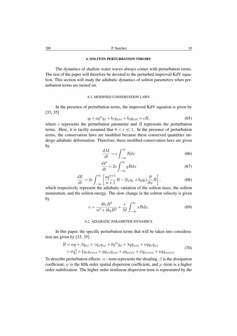
6. SOLITON PERTURBATION THEORY
The dynamics of shallow water waves always comes with perturbation terms.The rest of the paper will therefore be devoted to the perturbed improved KdV equa-tion. This section will study the adiabatic dynamics of soliton parameters when per-turbation terms are turned on.
6.1. MODIFIED CONSERVATION LAWS
In the presence of perturbation terms, the improved KdV equation is given by[33, 35]
qt+aqnqx+ b1qxxx+ b2qxxt = εR, (65)where ε represents the perturbation parameter and R represents the perturbationterms. Here, it is tacitly assumed that 0 < ε� 1. In the presence of perturbationterms, the conservation laws are modified because these conserved quantities un-dergo adiabatic deformation. Therefore, these modified conservation laws are givenby
dM
dt= ε
∫ ∞−∞
Rdx (66)
dP
dt= 2ε
∫ ∞−∞
qRdx (67)
dE
dt= 2ε
∫ ∞−∞
[aqn+1
n+ 1R− (b1qx+ b2qt)
∂
∂xR
], (68)
which respectively represent the adiabatic variation of the soliton mass, the solitonmomentum, and the soliton energy. The slow change in the soliton velocity is givenby
v =4b1B
2
n2 + 4b2B2+
ε
M
∫ ∞−∞
xRdx. (69)
6.2. ADIABATIC PARAMETER DYNAMICS
In this paper, the specific perturbation terms that will be taken into considera-tion are given by [33, 35]
R= αq+βqxx+γqxqxx+ δqmqx+λqqxxx+νqqxqxx
+σq3x+ ξqxqxxxx+ηqxxqxxx+ρqxxxx+ψqxxxxx+κqqxxxxx(70)
To describe perturbation effects: α - term represents the shoaling, β is the dissipationcoefficient, ψ is the fifth order spatial dispersion coefficient, and ρ -term is a higherorder stabilization. The higher order nonlinear dispersion term is represented by the
RJP 60(Nos. 3-4), 379–400 (2015) (c) 2015 - v.1.3a*2015.4.21

11 Cnoidal solutions, shock waves, solitary wave solutions of improved KdV equation 389
δ-term, where 1 ≤ m ≤ 4. The rest of the perturbation terms are described in theWhitham hierarchy.So, the perturbed equation considered in this paper is
qt+aqnqx+ b1qxxx+ b2qxxt
= ε(αq+βqxx+γqxqxx+ δqmqx+λqqxxx+νqqxqxx
+ σq3x+ ξqxqxxxx+ηqxxqxxx+ρqxxxx+ψqxxxxx+κqqxxxxx).
(71)
In the presence of these perturbation terms, the adiabatic change of the mass is givenby
dM
dt=εαA
B
Γ(12
)Γ(1n
)Γ(12 + 1
n
) = εαM, (72)
which shows thatM(t) =M0e
εαt, (73)where M0 is the initial mass of the soliton. Hence, in the limiting case
limt→∞
M(t) = 0, (74)
for α< 0. This shows that the mass adiabatically dissipates with time, in the presenceof shoaling since this is a dissipative perturbation term. The adiabatic change of themomentum is given by
dP
dt=
2εA2
Bn2(n+ 4)(3n+ 4)
Γ(12
)Γ(2n
)Γ(12 + 2
n
) ××{α(3n+ 4)(n+ 4)n2−4β(3n+ 4)nB2−16ρ(2n+ 3)B4
}.
(75)
This means that when dP/dt = 0, the solitons will travel with constant momentumfor a stable fixed value of the width given by
B =
[−βn(3n+ 4)
8ρ(2n+ 3)±n√
(3n+ 4)[β2(3n+ 4) + 4ρα(2n+ 3)(n+ 4)]
8ρ(2n+ 3)
] 12
, (76)
with the constraint condition
β2(3n+ 4)≥−4ρα(2n+ 3)(n+ 4). (77)
The corresponding fixed value of the amplitude, in this case by virtue of (24), is
A=
b1(n+ 1)(n+ 2)[−(3n+ 4)β±
√(3n+ 4)D1
]2a{
2ρn(2n+ 3) + b2
[−(3n+ 4)β±
√(3n+ 4)D1
]}
1n
, (78)
whereD1 = β2(3n+ 4) + 4ρα(2n+ 3)(n+ 4). (79)
RJP 60(Nos. 3-4), 379–400 (2015) (c) 2015 - v.1.3a*2015.4.21
390 P. Sanchez 12
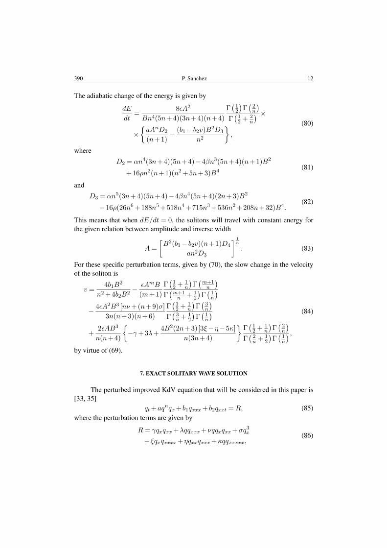
The adiabatic change of the energy is given by
dE
dt=
8εA2
Bn4(5n+ 4)(3n+ 4)(n+ 4)
Γ(12
)Γ(2n
)Γ(12 + 2
n
) ××{aAnD2
(n+ 1)− (b1− b2v)B2D3
n2
},
(80)
where
D2 = αn4(3n+ 4)(5n+ 4)−4βn3(5n+ 4)(n+ 1)B2
+ 16ρn2(n+ 1)(n2 + 5n+ 3)B4(81)
and
D3 = αn5(3n+ 4)(5n+ 4)−4βn4(5n+ 4)(2n+ 3)B2
−16ρ(26n6 + 188n5 + 518n4 + 715n3 + 536n2 + 208n+ 32)B4.(82)
This means that when dE/dt = 0, the solitons will travel with constant energy forthe given relation between amplitude and inverse width
A=
[B2(b1− b2v)(n+ 1)D4
an2D3
] 1n
. (83)
For these specific perturbation terms, given by (70), the slow change in the velocityof the soliton is
v =4b1B
2
n2 + 4b2B2− εAmB
(m+ 1)
Γ(12 + 1
n
)Γ(m+1n
)Γ(m+1n + 1
2
)Γ(1n
)− 4εA2B3 [nν+ (n+ 9)σ]
3n(n+ 3)(n+ 6)
Γ(12 + 1
n
)Γ(3n
)Γ(3n + 1
2
)Γ(1n
)+
2εAB3
n(n+ 4)
{−γ+ 3λ+
4B2(2n+ 3)[3ξ−η−5κ]
n(3n+ 4)
}Γ(12 + 1
n
)Γ(2n
)Γ(2n + 1
2
)Γ(1n
) ,(84)
by virtue of (69).
7. EXACT SOLITARY WAVE SOLUTION
The perturbed improved KdV equation that will be considered in this paper is[33, 35]
qt+aqnqx+ b1qxxx+ b2qxxt =R, (85)where the perturbation terms are given by
R= γqxqxx+λqqxxx+νqqxqxx+σq3x
+ ξqxqxxxx+ηqxxqxxx+κqqxxxxx,(86)
RJP 60(Nos. 3-4), 379–400 (2015) (c) 2015 - v.1.3a*2015.4.21
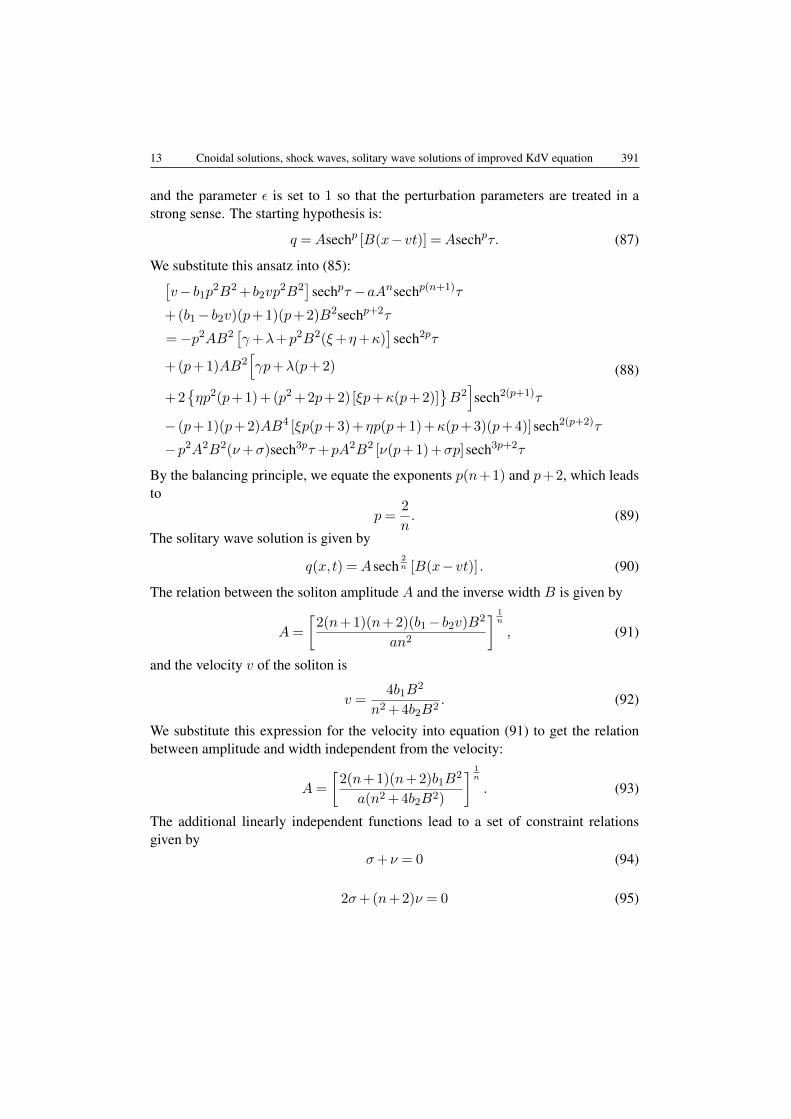
13 Cnoidal solutions, shock waves, solitary wave solutions of improved KdV equation 391
and the parameter ε is set to 1 so that the perturbation parameters are treated in astrong sense. The starting hypothesis is:
q =Asechp [B(x−vt)] =Asechpτ. (87)
We substitute this ansatz into (85):[v− b1p2B2 + b2vp
2B2]
sechpτ −aAnsechp(n+1)τ
+ (b1− b2v)(p+ 1)(p+ 2)B2sechp+2τ
=−p2AB2[γ+λ+p2B2(ξ+η+κ)
]sech2pτ
+ (p+ 1)AB2[γp+λ(p+ 2)
+ 2{ηp2(p+ 1) + (p2 + 2p+ 2)[ξp+κ(p+ 2)]
}B2]sech2(p+1)τ
− (p+ 1)(p+ 2)AB4 [ξp(p+ 3) +ηp(p+ 1) +κ(p+ 3)(p+ 4)]sech2(p+2)τ
−p2A2B2(ν+σ)sech3pτ +pA2B2 [ν(p+ 1) +σp]sech3p+2τ
(88)
By the balancing principle, we equate the exponents p(n+1) and p+2, which leadsto
p=2
n. (89)
The solitary wave solution is given by
q(x,t) =Asech2n [B(x−vt)] . (90)
The relation between the soliton amplitude A and the inverse width B is given by
A=
[2(n+ 1)(n+ 2)(b1− b2v)B2
an2
] 1n
, (91)
and the velocity v of the soliton is
v =4b1B
2
n2 + 4b2B2. (92)
We substitute this expression for the velocity into equation (91) to get the relationbetween amplitude and width independent from the velocity:
A=
[2(n+ 1)(n+ 2)b1B
2
a(n2 + 4b2B2)
] 1n
. (93)
The additional linearly independent functions lead to a set of constraint relationsgiven by
σ+ν = 0 (94)
2σ+ (n+ 2)ν = 0 (95)
RJP 60(Nos. 3-4), 379–400 (2015) (c) 2015 - v.1.3a*2015.4.21

392 P. Sanchez 14
This linear system of equations implies the unique solution[σν
]=
[00
]. (96)
The last set of constraint conditions is given by:
n2(γ+λ) + 4(ξ+η+κ)B2 = 0 (97)
n2(γ+ (n+ 1)λ) + 4{
(n2 + 2n+ 2)[ξ+ (n+ 1)κ] + (n+ 2)η}B2 = 0 (98)
(3n+ 2)ξ+ (n+ 2)η+ (3n+ 2)(2n+ 1)κ= 0. (99)This set of linear equations, given by (97)-(99) gives the solution
γλξηκ
=
−4(n+3)B2
n(3n+2)4(n+1)B2
n(3n+2)
− (n+2)(3n+2)
10
η+
−4B2
4(n+2)B2
n−(2n+ 1)
01
κ (100)
Thus, the system of linear equations (97)-(99) for the perturbation coefficients lead tothe conclusion that the five perturbation coefficients, ξ, η, κ, γ, and λ can be solvedin terms of two linearly independent parameters, namely η and κ only.
8. EXACT SINGULAR SOLITON SOLUTION
The starting hypothesis for the exact singular soliton solution is [35]:
q =Acschp [B(x−vt)] =Acschpτ. (101)
Substituting this ansatz into equation (85):[v− b1p2B2 + b2vp
2B2]
cschpτ −aAncschp(n+1)τ
+ (b1− b2v)(p+ 1)(p+ 2)B2cschp+2τ
=−p2AB2[γ+λ+p2B2(ξ+η+κ)
]csch2pτ
+ (p+ 1)AB2[γp+λ(p+ 2)
+ 2{ηp2(p+ 1) + (p2 + 2p+ 2)[ξp+κ(p+ 2)]
}B2]csch2(p+1)τ
− (p+ 1)(p+ 2)AB4 [ξp(p+ 3) +ηp(p+ 1) +κ(p+ 3)(p+ 4)]csch2(p+2)τ
−p2A2B2(ν+σ)csch3pτ +pA2B2 [ν(p+ 1) +σp]csch3p+2τ
(102)
RJP 60(Nos. 3-4), 379–400 (2015) (c) 2015 - v.1.3a*2015.4.21

15 Cnoidal solutions, shock waves, solitary wave solutions of improved KdV equation 393
Then balancing the exponents p(n+ 1) and p+ 2 leads to:
p=2
n. (103)
Finally, the singular soliton solution is given by:
q(x,t) =Acsch2n [B(x−vt)] . (104)
Note that the same expressions for the free parameter A and velocity v, which aregiven by (91)-(93), also apply for the singular soliton solution. The constraint condi-tions given by (94)-(100) for the perturbation terms considered for this problem holdas well.
9. EXACT SHOCK WAVE SOLUTION
The starting hypothesis for topological soliton solutions is as follows:
q =Atanhp [B(x−vt)] =Atanhp τ. (105)
We substitute this ansatz into (85):[v+ (b1− b2v)(3p2 + 3p+ 2)B2
]tanhp+1τ
−[v+ (b1− b2v)(3p2−3p+ 2)B2
]tanhp−1τ
+aAntanhp(n+1)−1τ −aAntanhp(n+1)+1τ
−[(b1− b2v)(p+ 1)(p+ 2)B2
]tanhp+3τ
+[(b1− b2v)(p−1)(p−2)B2
]tanhp−3τ
= (p−1)(p−2)AB4 [ξp(p−3) +ηp(p−1) +κ(p−3)(p−4)] tanh2p−5τ
− (p+ 1)(p+ 2)AB4 [ξp(p+ 3) +ηp(p+ 1) +κ(p+ 3)(p+ 4)] tanh2p+5τ
− (p+ 1)AB2[γp+λ(p+ 2)− ξp(5p2 + 13p+ 14)B2
− ηp(p+ 1)(5p+ 2)B2−5κ(p+ 2)(p2 + 3p+ 4)B2]
tanh2p+3τ
+ (p−1)AB2[γp+λ(p−2)− ξp(5p2−13p+ 14)B2
− ηp(p−1)(5p−2)B2−5κ(p−2)(p2−3p+ 4)B2]
tanh2p−3τ
−AB2[γp(3p−1) +λ(3p2−3p+ 2)−2ξp(5p3−6p2 + 13p−4)B2
− 2ηp2(5p2−4p+ 1)B2−2κ(5p4−10p3 + 25p2−20p+ 8)B2]
tanh2p−1τ
+AB2[γp(3p+ 1) +λ(3p2 + 3p+ 2)−2ξp(5p3 + 6p2 + 13p+ 4)B2
− 2ηp2(5p2 + 4p+ 1)B2−2κ(5p4 + 10p3 + 25p2 + 20p+ 8)B2]
tanh2p+1τ.
(106)
By the balancing principle we get
np+p+ 1 = p+ 3 (107)
RJP 60(Nos. 3-4), 379–400 (2015) (c) 2015 - v.1.3a*2015.4.21

394 P. Sanchez 16
np+p−1 = p+ 1 (108)
p=2
n(109)
From the coefficient of tanhp−3 τ
(b1− b2v)AB3p(p−1)(p−2) = 0 (110)
we can get two main cases.
9.1. CASE-I: p= 1, n= 2
The topological soliton solution of (85) is given by:
q =Atanh[B(x−vt)] . (111)
The velocity of the soliton is given by:
v =− 2b1B2
1−2b2B2. (112)
The relation between the free parameters A and B is given by:
A=
[−v+ 8(b1− b2v)B2
a
] 12
(113)
or
A=
[−6(b1− b2v)B2
a
] 12
(114)
These relations prompt the respective constraints given by
a{v+ 8(b1− b2v)B2
}< 0 (115)
anda{
(b1− b2v)B2}< 0 (116)
Upon equating eq. (113) and eq. (114) we can extract the same expression for thevelocity as in (112).The additional linearly independent functions lead to a set of constraint relationsgiven by:
σ = 0 (117)
2ν+ 3σ = 0 (118)
4ν+ 3σ = 0 (119)
RJP 60(Nos. 3-4), 379–400 (2015) (c) 2015 - v.1.3a*2015.4.21

17 Cnoidal solutions, shock waves, solitary wave solutions of improved KdV equation 395
2ν+σ = 0 (120)
γ+λ−2B2(4ξ+η+ 4κ) = 0 (121)
γ+ 2λ−B2(14ξ+ 5η+ 34κ) = 0 (122)
γ+ 3λ−2B2(16ξ+ 7η+ 60κ) = 0 (123)
2ξ+η+ 10κ= 0. (124)Equations (117)-(120) lead to a unique solution:[
σν
]=
[00
]. (125)
The system of linear equations (121)-(124) for the five perturbation coefficients, ξ,η, κ, γ, and λ can be solved in terms of only two linearly independent parameters ηand κ.
γλξηκ
=
−2B2
0−1
210
η+
−28B2
−4B2
−501
κ (126)
9.2. CASE-II: p= 2, n= 1
The topological soliton solution of (85) is given by:
q =Atanh2 [B(x−vt)] . (127)
The velocity of the soliton is given by:
v =−8b1B
2
1−8b2B2(128)
The relation between the free parameters A and B is given by:
A=−v+ 20(b1− b2v)B2
a(129)
or
A=−12(b1− b2v)B2
a. (130)
Upon equating these expressions we can extract the same expression for the velocityas in (128).
RJP 60(Nos. 3-4), 379–400 (2015) (c) 2015 - v.1.3a*2015.4.21
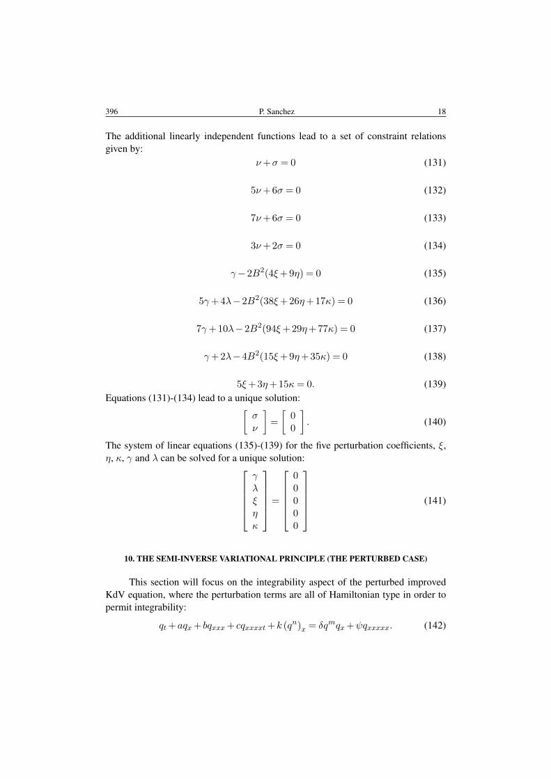
396 P. Sanchez 18
The additional linearly independent functions lead to a set of constraint relationsgiven by:
ν+σ = 0 (131)
5ν+ 6σ = 0 (132)
7ν+ 6σ = 0 (133)
3ν+ 2σ = 0 (134)
γ−2B2(4ξ+ 9η) = 0 (135)
5γ+ 4λ−2B2(38ξ+ 26η+ 17κ) = 0 (136)
7γ+ 10λ−2B2(94ξ+ 29η+ 77κ) = 0 (137)
γ+ 2λ−4B2(15ξ+ 9η+ 35κ) = 0 (138)
5ξ+ 3η+ 15κ= 0. (139)Equations (131)-(134) lead to a unique solution:[
σν
]=
[00
]. (140)
The system of linear equations (135)-(139) for the five perturbation coefficients, ξ,η, κ, γ and λ can be solved for a unique solution:
γλξηκ
=
00000
(141)
10. THE SEMI-INVERSE VARIATIONAL PRINCIPLE (THE PERTURBED CASE)
This section will focus on the integrability aspect of the perturbed improvedKdV equation, where the perturbation terms are all of Hamiltonian type in order topermit integrability:
qt+aqx+ bqxxx+ cqxxxxt+k (qn)x = δqmqx+ψqxxxxx. (142)
RJP 60(Nos. 3-4), 379–400 (2015) (c) 2015 - v.1.3a*2015.4.21

19 Cnoidal solutions, shock waves, solitary wave solutions of improved KdV equation 397
The traveling wave hypothesis is taken to be
q(x,t) = g(x−vt) = g(s), (143)
wheres= x−vt. (144)
Substituting this traveling wave assumption into (142) and integrating once whiletaking the integration constant to be zero gives
−vg+a
n+ 1gn+1 +
δ
m+ 1gm+1 + (b1− b2v)g′′+ψg′′′′ = 0. (145)
Now, multiplying both sides of (145) by g′ and integrating leads to
− v2g2 +
a
(n+ 1)(n+ 2)gn+2 +
b1− b2v2
(g′)2
+δ
(m+ 1)(m+ 2)gm+2 +ψ
[g′g′′′− 1
2(g′′)2
]=K,
(146)
where K is the integration constant. The stationary integral is then defined as
J =
∫ ∞−∞
Kds
=
∫ ∞−∞
[−v
2g2 +
a
(n+ 1)(n+ 2)gn+2 +
b1− b2v2
(g′)2
+δ
(m+ 1)(m+ 2)gm+2 +ψ
[g′g′′′− 1
2(g′′)2
]]ds.
(147)
Now, choosing
g(s) =Asech2n (Bs) (148)
as a solution hypothesis for (142), where A and B are still the amplitude and inversewidth of the soliton, the stationary integral J reduces to
J =A2
2B
Γ(12
)Γ(2n
)Γ(12 + 2
n
) { 8aAn
(n+ 1)(n+ 2)(n+ 4)−v+
4(b1− b2v)B2
(n+ 4)n
+16ψ(2n+ 3)B4
(n+ 4)(3n+ 4)n2
}+
δAm+2
(m+ 1)(m+ 2)B
Γ(12
)Γ(m+2n
)Γ(12 + m+2
n
) . (149)
Then SVP gives
∂J
∂A=A
B
Γ(12
)Γ(2n
)Γ(12 + 2
n
) { 4aAn
(n+ 1)(n+ 4)−v+
4(b1− b2v)B2
(n+ 4)n
+16ψ(2n+ 3)B4
(n+ 4)(3n+ 4)n2
}+
δAm+1
(m+ 1)B
Γ(12
)Γ(m+2n
)Γ(12 + m+2
n
) = 0
(150)
RJP 60(Nos. 3-4), 379–400 (2015) (c) 2015 - v.1.3a*2015.4.21

398 P. Sanchez 20
and
∂J
∂B=A2
2
Γ(12
)Γ(2n
)Γ(12 + 2
n
) { −8aAn
(n+ 1)(n+ 2)(n+ 4)B2+
v
B2+
4(b1− b2v)
(n+ 4)n
+48ψ(2n+ 3)B2
(n+ 4)(3n+ 4)n2
}− δAm+2
(m+ 1)(m+ 2)B2
Γ(12
)Γ(m+2n
)Γ(12 + m+2
n
) = 0,
(151)
which leads to the amplitude-width relationship given by
A=
[− (n+ 1)(n+ 2)
8a(3n+ 4)n2(n−m)×
×{mv(n+ 4)(3n+ 4)n2 + 4(b1− b2v)(3n+ 4)n(m+ 4)B2
+ 16ψ(2n+ 3)(3m+ 8)B4}] 1
m .
(152)
11. CONCLUSIONS
In this paper we have obtained exact solitary-wave, shock-wave, and cnoidal-wave solutions of the improved Korteweg-de Vries equation with power law nonli-nearity. Additionally, the soliton perturbation theory recovered adiabatic dynamicsof soliton parameters. These results will be further generalized. The improvedKorteweg-de Vries equation with time-dependent coefficients will be studied. Thestochastic perturbation terms will be applied and the dynamics of soliton parameters,in the presence of random perturbations will be investigated. Those new results willbe reported elsewhere.
REFERENCES
1. R. Abazari, Romanian Journal of Physics 59 (1–2), 3–11 (2014).2. R. Abazari, Romanian Reports in Physics 66 (2), 286–295 (2014).3. M. Ablowitz and H. Segur, Solitons and the Inverse Scattering Transform, Studies in Applied
Mathematics, SIAM, Philadelphia, 1981.4. M. Antonova and A. Biswas, Communications in Nonlinear Science and Numerical Simulation 14
(3), 734–748 (2009).5. A.H. Bhrawy, A.A. Alshaery, E.M. Hilal, D. Milovic, L. Moraru, M. Savescu, and A. Biswas,
Proceedings of the Romanian Academy, Series A 15 (3), 235–240 (2014).6. A.H. Bhrawy, M.A. Abdelkawy, S. Kumar, and A. Biswas, Romanian Journal of Physics 58 (7–8),
729–748 (2013).7. A. Biswas, Nonlinear Dynamics 59 (3), 423–426 (2010).8. A. Biswas, Communications in Nonlinear Science and Numerical Simulation 14 (9–10), 3503–
3506 (2009).9. A. Biswas and M. Ismail, Applied Mathematics and Computation 216 (12), 3662–3670 (2010).
10. A. Biswas, E. Krishnan, P. Suarez, A. Kara, and S. Kumar, Indian Journal of Physics 87 (2), 169–175 (2013).
RJP 60(Nos. 3-4), 379–400 (2015) (c) 2015 - v.1.3a*2015.4.21

21 Cnoidal solutions, shock waves, solitary wave solutions of improved KdV equation 399
11. A. Biswas, M. Song, H. Triki, A. H. Kara, B. S. Ahmed, A. Strong, and A. Hama, Applied Math-ematics and Information Sciences 8 (3), 949–957 (2014).
12. A. Biswas, H. Triki, and M. Labidi, Physics of Wave Phenomena 19 (1), 24–29 (2011).13. Z.G. Chen, M. Segev, and D.N. Christodoulides, Reports on Progress in Physics 75 (8), 086401
(2012).14. R. Cimpoiasu, Rom. J. Phys. 59 (7–8), 617-624 (2014).15. E.H. Doha, A.H. Bhrawy, D. Baleanu, and M. A. Abdelkawy, Romanian Journal of Physics 59
(3–4), 247–264 (2014).16. D.J. Frantzeskakis, H. Leblond, and D. Mihalache, Romanian Journal of Physics 59 (7–8), 767–
784 (2014).17. A.G. Johnpillai, A.H. Kara, and A. Biswas, Applied Mathematics Letters 26 (3), 376–381 (2013).18. Y.V. Kartashov, B.A. Malomed, and L. Torner, Reviews of Modern Physics 83 (1), 247–305 (2011).19. Y. Kodama and M. Ablowitz, Studies in Applied Mathematics 64, 225–245 (1981).20. E.V. Krishnan, S. Kumar, and A. Biswas, Nonlinear Dynamics 70 (2), 1213–1221 (2012).21. S. Kumar, A. Hama, and A. Biswas, Applied Mathematics and Infromation Sciences 8 (4), 1533–
1539 (2014).22. S. Kutluay and A. Esen, International Journal of Nonlinear Sciences and Numerical Simulations
10 (6), 717–725 (2009).23. M. Labidi and A. Biswas, Mathematics in Engineering, Science and Aerospace 2 (2), 183–197
(2011).24. H. Leblond, H. Triki, and D. Mihalache, Romanian Reports in Physics 65 (3), 925–942 (2013).25. H. Leblond and D. Mihalache, Physics Reports-Review Section of Physics Letters 523 (2), 61–126
(2013).26. B.A. Malomed, D. Mihalache, F. Wise, and L. Torner, Journal of Optics B: Quantum and Semi-
classical Optics 7 (5), R53–R72 (2005).27. D. Mihalache, Romanian Journal of Physics 57 (1–2), 352–371 (2012).28. D. Mihalache, Romanian Journal of Physics 59 (3–4), 295–312 (2014).29. D. Mihalache, D. Mazilu, F. Lederer, and Y.S. Kivshar, Optics Express 15 (2), 589–595 (2007).30. D. Mihalache, D. Mazilu, F. Lederer, and Y.S. Kivshar, Optics Letters 32 (21), 3173–3175 (2007).31. R. Morris, A.H. Kara, A. Chowdhury, and A. Biswas, Zeitschrift fur Naturforschung A 67a, 613–
620 (2012).32. R. Radha, P.S. Vinayagam, and K. Porsezian, Romanian Reports in Physics 66 (2), 427–442
(2014).33. P. Razborova, H. Triki, and A. Biswas, Ocean Engineering 63, 1–7 (2013).34. P. Razborova, B. Ahmed, and A. Biswas, Applied Mathematics and Information Sciences 8 (2),
485–491 (2014).35. P. Razborova, L. Moraru, and A. Biswas, Romanian Journal of Physics 59 (7–8), 658–676 (2014).36. M. Savescu, A.H. Bhrawy, A.A. Alshaery, E.M. Hilal, K. Khan, M.F. Mahmood, and A. Biswas,
J. Modern Optics 61 (5), 441–458 (2014).37. H. Triki, Romanian Journal of Physics 59 (5–6), 421–432 (2014).38. H. Triki, A. Kara, A. Bhrawy, and A. Biswas, Acta Physica Polonica A 125 (5), 1099–1106 (2014).39. H. Triki, M. Mirzazadeh, A.H. Bhrawy, P. Razborova, and A. Biswas, Romanian Journal of Physics
60, 72–86 (2015).40. G. Wang, T. Xu, G. Ebadi, S. Johnson, A. Strong, and A. Biswas, Nonlinear Dynamics 76 (2),
1059–1068 (2014).41. A. Wazwaz, Proceedings of the Romanian Academy, Series A 15 (3), 241–246 (2014).
RJP 60(Nos. 3-4), 379–400 (2015) (c) 2015 - v.1.3a*2015.4.21

400 P. Sanchez 22
42. A. Wazwaz and A. Ebaid, Romanian Journal of Physics 59 (5–6), 454–465 (2014).43. A. Wazwaz, Applied Mathematics and Computation 219, 2535–2544 (2012).44. A. Wazwaz, Applied Mathematics and Computation 204, 162–169 (2008).45. A. Wazwaz, Applied Mathematics and Computation 187, 1131–1142 (2007).46. A. Wazwaz, Applied Mathematics and Computation 184, 1002–1014 (2007).47. Y. Xue, F.W. Ye, D. Mihalache, N.C. Panoiu, and X.F. Chen, Laser and Photonics Reviews 8 (4),
L52–L57 (2014).48. G.Y. Yang, L. Li, S.T. Jia, and D. Mihalache, Romanian Reports in Physics 65 (2), 391–400 (2013).49. G.Y. Yang, L. Li, S.T. Jia, and D. Mihalache, Romanian Reports in Physics 65 (3), 902–914 (2013).50. F.W. Ye, D. Mihalache, B.B. Hu, and N.C.Panoiu, Physical Review Letters 104 (10), 106802
(2010).51. L. Zhang and A. Chen, Proceedings of the Romanian Academy, Series A 15 (1), 11–17 (2014).52. Z. Zhang, J. Zhong, S. S. Dou, J. Liu, D. Peng, and T. Gao, Romanian Reports in Physics 65 (4),
1155–1169 (2013).
RJP 60(Nos. 3-4), 379–400 (2015) (c) 2015 - v.1.3a*2015.4.21