package 'signal

Package ‘signal’July 30, 2015

Title Signal Processing

Version 0.7-6

Date 2015-07-29

Depends R (>= 2.14.0)

Imports MASS, graphics, grDevices, stats, utils

Suggests pracma

Description A set of signal processing functions originally written for 'Matlab' and 'Octave'.Includes filter generation utilities, filtering functions,resampling routines, and visualization of filter models. It alsoincludes interpolation functions.

License GPL-2

NeedsCompilation yes

Author Uwe Ligges [aut, cre] (new maintainer),Tom Short [aut] (port to R),Paul Kienzle [aut] (majority of the original sources),Sarah Schnackenberg [ctb] (various test cases and bug fixes),David Billinghurst [ctb],Hans-Werner Borchers [ctb],Andre Carezia [ctb],Pascal Dupuis [ctb],John W. Eaton [ctb],E. Farhi [ctb],Kai Habel [ctb],Kurt Hornik [ctb],Sebastian Krey [ctb],Bill Lash [ctb],Friedrich Leisch [ctb],Olaf Mersmann [ctb],Paulo Neis [ctb],Jaakko Ruohio [ctb],Julius O. Smith III [ctb],Doug Stewart [ctb],Andreas Weingessel [ctb]

1

2 R topics documented:

Maintainer Uwe Ligges <[email protected]>

Repository CRAN

Date/Publication 2015-07-30 00:17:37

R topics documented:signal-package . . . . . . . . . . . . . . . . . . . . . . . . . . . . . . . . . . . . . . . 3an . . . . . . . . . . . . . . . . . . . . . . . . . . . . . . . . . . . . . . . . . . . . . . 4Arma . . . . . . . . . . . . . . . . . . . . . . . . . . . . . . . . . . . . . . . . . . . . 5bilinear . . . . . . . . . . . . . . . . . . . . . . . . . . . . . . . . . . . . . . . . . . . 6butter . . . . . . . . . . . . . . . . . . . . . . . . . . . . . . . . . . . . . . . . . . . . 8buttord . . . . . . . . . . . . . . . . . . . . . . . . . . . . . . . . . . . . . . . . . . . . 10cheb1ord . . . . . . . . . . . . . . . . . . . . . . . . . . . . . . . . . . . . . . . . . . 11chebwin . . . . . . . . . . . . . . . . . . . . . . . . . . . . . . . . . . . . . . . . . . . 12cheby1 . . . . . . . . . . . . . . . . . . . . . . . . . . . . . . . . . . . . . . . . . . . . 14chirp . . . . . . . . . . . . . . . . . . . . . . . . . . . . . . . . . . . . . . . . . . . . . 16conv . . . . . . . . . . . . . . . . . . . . . . . . . . . . . . . . . . . . . . . . . . . . . 17decimate . . . . . . . . . . . . . . . . . . . . . . . . . . . . . . . . . . . . . . . . . . . 18ellip . . . . . . . . . . . . . . . . . . . . . . . . . . . . . . . . . . . . . . . . . . . . . 19ellipord . . . . . . . . . . . . . . . . . . . . . . . . . . . . . . . . . . . . . . . . . . . 21fftfilt . . . . . . . . . . . . . . . . . . . . . . . . . . . . . . . . . . . . . . . . . . . . . 22filter . . . . . . . . . . . . . . . . . . . . . . . . . . . . . . . . . . . . . . . . . . . . . 23FilterOfOrder . . . . . . . . . . . . . . . . . . . . . . . . . . . . . . . . . . . . . . . . 25filtfilt . . . . . . . . . . . . . . . . . . . . . . . . . . . . . . . . . . . . . . . . . . . . 26fir1 . . . . . . . . . . . . . . . . . . . . . . . . . . . . . . . . . . . . . . . . . . . . . . 27fir2 . . . . . . . . . . . . . . . . . . . . . . . . . . . . . . . . . . . . . . . . . . . . . . 28freqs . . . . . . . . . . . . . . . . . . . . . . . . . . . . . . . . . . . . . . . . . . . . . 29freqz . . . . . . . . . . . . . . . . . . . . . . . . . . . . . . . . . . . . . . . . . . . . . 31grpdelay . . . . . . . . . . . . . . . . . . . . . . . . . . . . . . . . . . . . . . . . . . . 33ifft . . . . . . . . . . . . . . . . . . . . . . . . . . . . . . . . . . . . . . . . . . . . . . 35impz . . . . . . . . . . . . . . . . . . . . . . . . . . . . . . . . . . . . . . . . . . . . . 36interp . . . . . . . . . . . . . . . . . . . . . . . . . . . . . . . . . . . . . . . . . . . . 37interp1 . . . . . . . . . . . . . . . . . . . . . . . . . . . . . . . . . . . . . . . . . . . . 38kaiser . . . . . . . . . . . . . . . . . . . . . . . . . . . . . . . . . . . . . . . . . . . . 40kaiserord . . . . . . . . . . . . . . . . . . . . . . . . . . . . . . . . . . . . . . . . . . 41levinson . . . . . . . . . . . . . . . . . . . . . . . . . . . . . . . . . . . . . . . . . . . 43Ma . . . . . . . . . . . . . . . . . . . . . . . . . . . . . . . . . . . . . . . . . . . . . . 44medfilt1 . . . . . . . . . . . . . . . . . . . . . . . . . . . . . . . . . . . . . . . . . . . 44pchip . . . . . . . . . . . . . . . . . . . . . . . . . . . . . . . . . . . . . . . . . . . . 46poly . . . . . . . . . . . . . . . . . . . . . . . . . . . . . . . . . . . . . . . . . . . . . 47polyval . . . . . . . . . . . . . . . . . . . . . . . . . . . . . . . . . . . . . . . . . . . 48remez . . . . . . . . . . . . . . . . . . . . . . . . . . . . . . . . . . . . . . . . . . . . 48resample . . . . . . . . . . . . . . . . . . . . . . . . . . . . . . . . . . . . . . . . . . . 49roots . . . . . . . . . . . . . . . . . . . . . . . . . . . . . . . . . . . . . . . . . . . . . 51sftrans . . . . . . . . . . . . . . . . . . . . . . . . . . . . . . . . . . . . . . . . . . . . 52sgolay . . . . . . . . . . . . . . . . . . . . . . . . . . . . . . . . . . . . . . . . . . . . 55sgolayfilt . . . . . . . . . . . . . . . . . . . . . . . . . . . . . . . . . . . . . . . . . . 56

signal-package 3

signal-internal . . . . . . . . . . . . . . . . . . . . . . . . . . . . . . . . . . . . . . . . 57specgram . . . . . . . . . . . . . . . . . . . . . . . . . . . . . . . . . . . . . . . . . . 58spencer . . . . . . . . . . . . . . . . . . . . . . . . . . . . . . . . . . . . . . . . . . . 60unwrap . . . . . . . . . . . . . . . . . . . . . . . . . . . . . . . . . . . . . . . . . . . 61wav . . . . . . . . . . . . . . . . . . . . . . . . . . . . . . . . . . . . . . . . . . . . . 61Windowing functions . . . . . . . . . . . . . . . . . . . . . . . . . . . . . . . . . . . . 62Zpg . . . . . . . . . . . . . . . . . . . . . . . . . . . . . . . . . . . . . . . . . . . . . 64zplane . . . . . . . . . . . . . . . . . . . . . . . . . . . . . . . . . . . . . . . . . . . . 65

Index 67

signal-package Signal processing

Description

A set of generally Matlab/Octave-compatible signal processing functions. Includes filter generationutilities, filtering functions, resampling routines, and visualization of filter models. It also includesinterpolation functions and some Matlab compatibility functions.

Details

The main routines are:

Filtering: filter, fftfilt, filtfilt, medfilt1, sgolay, sgolayfilt

Resampling: interp, resample, decimate

IIR filter design: bilinear, butter, buttord, cheb1ord, cheb2ord, cheby1, cheby2, ellip, ellipord,sftrans

FIR filter design: fir1, fir2, remez, kaiserord, spencer

Interpolation: interp1, pchip

Compatibility routines and utilities: ifft, sinc, postpad, chirp, poly, polyval

Windowing: bartlett, blackman, boxcar, flattopwin, gausswin, hamming, hanning, triang

Analysis and visualization: freqs, freqz, impz, zplane, grpdelay, specgram

Most of the functions accept Matlab-compatible argument lists, but many are generic functions andcan accept simpler argument lists.

For a complete list, use library(help="signal").

Author(s)

Most of these routines were translated from Octave Forge routines. The main credit goes to theoriginal Octave authors:

Paul Kienzle, John W. Eaton, Kurt Hornik, Andreas Weingessel, Kai Habel, Julius O. Smith III, BillLash, André Carezia, Paulo Neis, David Billinghurst, Friedrich Leisch

Translations by Tom Short <[email protected]> (who maintained the package until2009).

Current maintainer is Uwe Ligges <[email protected]>.

4 an

References

http://en.wikipedia.org/wiki/Category:Signal_processing

Octave Forge http://octave.sf.net

Package matlab by P. Roebuck

For Matlab/Octave conversion and compatibility, see http://mathesaurus.sourceforge.net/octave-r.html by Vidar Bronken Gundersen and http://cran.r-project.org/doc/contrib/R-and-octave.txt by Robin Hankin.

Examples

## The R implementation of these routines can be called "matlab-style",bf <- butter(5, 0.2)freqz(bf$b, bf$a)## or "R-style" as:freqz(bf)

## make a Chebyshev type II filter:ch <- cheby2(5, 20, 0.2)freqz(ch, Fs = 100) # frequency plot for a sample rate = 100 Hz

zplane(ch) # look at the poles and zeros

## apply the filter to a signalt <- seq(0, 1, by = 0.01) # 1 second sample, Fs = 100 Hzx <- sin(2*pi*t*2.3) + 0.25*rnorm(length(t)) # 2.3 Hz sinusoid+noisez <- filter(ch, x) # apply filterplot(t, x, type = "l")lines(t, z, col = "red")

# look at the group delay as a function of frequencygrpdelay(ch, Fs = 100)

an Complex unit phasor of the given angle in degrees.

Description

Complex unit phasor of the given angle in degrees.

Usage

an(degrees)

Arguments

degrees Angle in degrees.

http://en.wikipedia.org/wiki/Category:Signal_processing

http://octave.sf.net

http://mathesaurus.sourceforge.net/octave-r.html

http://mathesaurus.sourceforge.net/octave-r.html

http://cran.r-project.org/doc/contrib/R-and-octave.txt

http://cran.r-project.org/doc/contrib/R-and-octave.txt

Arma 5

Details

This is a utility function to make it easier to specify phasor values as a magnitude times an angle indegrees.

Value

A complex value or array of exp(1i*degrees*pi/180).

Examples

120*an(30) + 125*an(-160)

Arma Create an autoregressive moving average (ARMA) model.

Description

Returns an ARMA model. The model could represent a filter or system model.

Usage

Arma(b, a)

## S3 method for class 'Zpg'as.Arma(x, ...)

## S3 method for class 'Arma'as.Arma(x, ...)

## S3 method for class 'Ma'as.Arma(x, ...)

Arguments

b moving average (MA) polynomial coefficients.

a autoregressive (AR) polynomial coefficients.

x model or filter to be converted to an ARMA representation.

... additional arguments (ignored).

Details

The ARMA model is defined by:

a(L)y(t) = b(L)x(t)

6 bilinear

The ARMA model can define an analog or digital model. The AR and MA polynomial coefficientsfollow the Matlab/Octave convention where the coefficients are in decreasing order of the polyno-mial (the opposite of the definitions for filter from the stats package and polyroot from the basepackage). For an analog model,

H(s) =b1s

m−1 + b2sm−2 + . . .+ bm

a1sn−1 + a2sn−2 + . . .+ an

For a z-plane digital model,

H(z) =b1 + b2z

−1 + . . .+ bmz−m+1

a1 + a2z−1 + . . .+ anz−n+1

as.Arma converts from other forms, including Zpg and Ma.

Value

A list of class Arma with the following list elements:

b moving average (MA) polynomial coefficients

a autoregressive (AR) polynomial coefficients

Author(s)

Tom Short, EPRI Solutions, Inc., (<[email protected]>)

See Also

See also as.Zpg, Ma, filter, and various filter-generation functions like butter and cheby1 thatreturn Arma models.

Examples

filt <- Arma(b = c(1, 2, 1)/3, a = c(1, 1))zplane(filt)

bilinear Bilinear transformation

Description

Transform a s-plane filter specification into a z-plane specification.

bilinear 7

Usage

## Default S3 method:bilinear(Sz, Sp, Sg, T, ...)

## S3 method for class 'Zpg'bilinear(Sz, T, ...)

## S3 method for class 'Arma'bilinear(Sz, T, ...)

Arguments

Sz In the generic case, a model to be transformed. In the default case, a vectorcontaining the zeros in a pole-zero-gain model.

Sp a vector containing the poles in a pole-zero-gain model.

Sg a vector containing the gain in a pole-zero-gain model.

T the sampling frequency represented in the z plane.

... Arguments passed to the generic function.

Details

Given a piecewise flat filter design, you can transform it from the s-plane to the z-plane whilemaintaining the band edges by means of the bilinear transform. This maps the left hand side of thes-plane into the interior of the unit circle. The mapping is highly non-linear, so you must design yourfilter with band edges in the s-plane positioned at 2/T tan(w ∗ T/2) so that they will be positionedat w after the bilinear transform is complete.

The bilinear transform is:

z =1 + sT/2

1− sT/2

s =T

2

z − 1

z + 1

Please note that a pole and a zero at the same place exactly cancel. This is significant since thebilinear transform creates numerous extra poles and zeros, most of which cancel. Those which donot cancel have a “fill-in” effect, extending the shorter of the sets to have the same number of asthe longer of the sets of poles and zeros (or at least split the difference in the case of the band passfilter). There may be other opportunistic cancellations, but it will not check for them.

Also note that any pole on the unit circle or beyond will result in an unstable filter. Because ofcancellation, this will only happen if the number of poles is smaller than the number of zeros. Theanalytic design methods all yield more poles than zeros, so this will not be a problem.

8 butter

Value

For the default case or for bilinear.Zpg, an object of class “Zpg”, containing the list elements:

zero complex vector of the zeros of the transformed model

pole complex vector of the poles of the transformed model

gain gain of the transformed model

For bilinear.Arma, an object of class “Arma”, containing the list elements:



Author(s)

Original Octave version by Paul Kienzle <[email protected]>. Conversion to R by TomShort.

References

Proakis & Manolakis (1992). Digital Signal Processing. New York: Macmillan Publishing Com-pany.

http://en.wikipedia.org/wiki/Bilinear_transform


See Also

Zpg, sftrans, Arma

butter Generate a Butterworth filter.

Description

Generate Butterworth filter polynomial coefficients.

Usage

## Default S3 method:butter(n, W, type = c("low", "high", "stop", "pass"),plane = c("z", "s"), ...)

## S3 method for class 'FilterOfOrder'butter(n, ...)

http://en.wikipedia.org/wiki/Bilinear_transform


butter 9

Arguments

n filter order or generic filter model

W critical frequencies of the filter. W must be a scalar for low-pass and high-passfilters, and W must be a two-element vector c(low, high) specifying the lowerand upper bands. For digital filters, W must be between 0 and 1 where 1 is theNyquist frequency.

type Filter type, one of "low" for a low-pass filter, "high" for a high-pass filter,"stop" for a stop-band (band-reject) filter, or "pass" for a pass-band filter.

plane "z" for a digital filter or "s" for an analog filter.

... additional arguments passed to butter, overriding those given by n of classFilterOfOrder.

Details

Because butter is generic, it can be extended to accept other inputs, using "buttord" to generatefilter criteria for example.

Value

An Arma object with list elements:



Author(s)

Original Octave version by Paul Kienzle <[email protected]>. Modified by Doug Stewart.Conversion to R by Tom Short.

References


http://en.wikipedia.org/wiki/Butterworth_filter


See Also

Arma, filter, cheby1, ellip, and buttord

Examples

bf <- butter(4, 0.1)freqz(bf)zplane(bf)

http://en.wikipedia.org/wiki/Butterworth_filter


10 buttord

buttord Butterworth filter order and cutoff

Description

Compute butterworth filter order and cutoff for the desired response characteristics.

Usage

buttord(Wp, Ws, Rp, Rs)

Arguments

Wp, Ws pass-band and stop-band edges. For a low-pass or high-pass filter, Wp and Wsare scalars. For a band-pass or band-rejection filter, both are vectors of length2. For a low-pass filter, Wp < Ws. For a high-pass filter, Ws > Wp. Fora band-pass (Ws[1] < Wp[1] < Wp[2] < Ws[2]) or band-reject(Wp[1] < Ws[1] < Ws[2] < Wp[2]) filter design, Wp gives the edges of thepass band, and Ws gives the edges of the stop band. Frequencies are normalizedto [0,1], corresponding to the range [0, Fs/2].

Rp allowable decibels of ripple in the pass band.

Rs minimum attenuation in the stop band in dB.

Details

Deriving the order and cutoff is based on:

|H(W )|2 =1

1 + (W/Wc)2n= 10−R/10

With some algebra, you can solve simultaneously for Wc and n given Ws, Rs and Wp, Rp. For high-pass filters, subtracting the band edges from Fs/2, performing the test, and swapping the resulting Wcback works beautifully. For bandpass- and bandstop-filters, this process significantly overdesigns.Artificially dividing n by 2 in this case helps a lot, but it still overdesigns.

Value

An object of class FilterOfOrder with the following list elements:

n filter order

Wc cutoff frequency

type filter type, one of “low”, “high”, “stop”, or “pass”

This object can be passed directly to butter to compute filter coefficients.

cheb1ord 11

Author(s)

Original Octave version by Paul Kienzle, <[email protected]>. Conversion to R by TomShort.

References


See Also

butter, FilterOfOrder, cheb1ord

Examples

Fs <- 10000btord <- buttord(1000/(Fs/2), 1200/(Fs/2), 0.5, 29)plot(c(0, 1000, 1000, 0, 0), c(0, 0, -0.5, -0.5, 0),

type = "l", xlab = "Frequency (Hz)", ylab = "Attenuation (dB)")bt <- butter(btord)plot(c(0, 1000, 1000, 0, 0), c(0, 0, -0.5, -0.5, 0),

type = "l", xlab = "Frequency (Hz)", ylab = "Attenuation (dB)",col = "red", ylim = c(-10,0), xlim = c(0,2000))

hf <- freqz(bt, Fs = Fs)lines(hf$f, 20*log10(abs(hf$h)))

cheb1ord Chebyshev type-I filter order and cutoff

Description

Compute discrete Chebyshev type-I filter order and cutoff for the desired response characteristics.

Usage

cheb1ord(Wp, Ws, Rp, Rs)

Arguments





12 chebwin

Value


n filter order

Wc cutoff frequency

Rp allowable decibels of ripple in the pass band

type filter type, one of “low”, “high”, “stop”, or “pass”

This object can be passed directly to cheby1 to compute filter coefficients.

Author(s)

Original Octave version by Paul Kienzle, <[email protected]> and by Laurent S. Mazet.Conversion to R by Tom Short.

References


See Also

cheby1, FilterOfOrder, buttord

Examples

Fs <- 10000chord <- cheb1ord(1000/(Fs/2), 1200/(Fs/2), 0.5, 29)plot(c(0, 1000, 1000, 0, 0), c(0, 0, -0.5, -0.5, 0),

type = "l", xlab = "Frequency (Hz)", ylab = "Attenuation (dB)")ch1 <- cheby1(chord)plot(c(0, 1000, 1000, 0, 0), c(0, 0, -0.5, -0.5, 0),


hf <- freqz(ch1, Fs = Fs)lines(hf$f, 20*log10(abs(hf$h)))

chebwin Dolph-Chebyshev window coefficients

Description

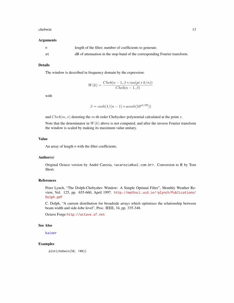
Returns the filter coefficients of the n-point Dolph-Chebyshev window with a given attenuation.

Usage

chebwin(n, at)


chebwin 13

Arguments

n length of the filter; number of coefficients to generate.

at dB of attenuation in the stop-band of the corresponding Fourier transform.

Details

The window is described in frequency domain by the expression:

W (k) =Cheb(n− 1, β ∗ cos(pi ∗ k/n))

Cheb(n− 1, β)

with

β = cosh(1/(n− 1) ∗ acosh(10at/20))

and Cheb(m,x) denoting the m-th order Chebyshev polynomial calculated at the point x.

Note that the denominator in W (k) above is not computed, and after the inverse Fourier transformthe window is scaled by making its maximum value unitary.

Value

An array of length n with the filter coefficients.

Author(s)

Original Octave version by André Carezia, <[email protected]>. Conversion to R by TomShort.

References

Peter Lynch, “The Dolph-Chebyshev Window: A Simple Optimal Filter”, Monthly Weather Re-view, Vol. 125, pp. 655-660, April 1997. http://mathsci.ucd.ie/~plynch/Publications/Dolph.pdf

C. Dolph, “A current distribution for broadside arrays which optimizes the relationship betweenbeam width and side-lobe level”, Proc. IEEE, 34, pp. 335-348.


See Also

kaiser

Examples

plot(chebwin(50, 100))

http://mathsci.ucd.ie/~plynch/Publications/Dolph.pdf

http://mathsci.ucd.ie/~plynch/Publications/Dolph.pdf


14 cheby1

cheby1 Generate a Chebyshev filter.

Description

Generate a Chebyshev type I or type II filter coefficients with specified dB of pass band ripple.

Usage

## Default S3 method:cheby1(n, Rp, W, type = c("low", "high", "stop","pass"), plane = c("z", "s"), ...)

## S3 method for class 'FilterOfOrder'cheby1(n, Rp = n$Rp, W = n$Wc, type = n$type, ...)

## Default S3 method:cheby2(n, Rp, W, type = c("low", "high", "stop","pass"), plane = c("z", "s"), ...)

## S3 method for class 'FilterOfOrder'cheby2(n, ...)

Arguments


Rp dB of pass band ripple




... additional arguments passed to cheby1 or cheby2, overriding those given by nof class FilterOfOrder.

Details

Because cheby1 and cheby2 are generic, they can be extended to accept other inputs, using "cheb1ord"to generate filter criteria for example.

cheby1 15

Value




For cheby1, the ARMA model specifies a type-I Chebyshev filter, and for cheby2, a type-II Cheby-shev filter.

Author(s)

Original Octave version by Paul Kienzle <[email protected]>. Modified by Doug Stewart.Conversion to R by Tom Short.

References

Parks & Burrus (1987). Digital Filter Design. New York: John Wiley & Sons, Inc.

http://en.wikipedia.org/wiki/Chebyshev_filter


See Also

Arma, filter, butter, ellip, and cheb1ord

Examples

# compare the frequency responses of 5th-order Butterworth and Chebyshev filters.bf <- butter(5, 0.1)cf <- cheby1(5, 3, 0.1)bfr <- freqz(bf)cfr <- freqz(cf)plot(bfr$f/pi, 20 * log10(abs(bfr$h)), type = "l", ylim = c(-40, 0),

xlim = c(0, .5), xlab = "Frequency", ylab = c("dB"))lines(cfr$f/pi, 20 * log10(abs(cfr$h)), col = "red")# compare type I and type II Chebyshev filters.c1fr <- freqz(cheby1(5, .5, 0.5))c2fr <- freqz(cheby2(5, 20, 0.5))plot(c1fr$f/pi, abs(c1fr$h), type = "l", ylim = c(0, 1),

xlab = "Frequency", ylab = c("Magnitude"))lines(c2fr$f/pi, abs(c2fr$h), col = "red")

http://en.wikipedia.org/wiki/Chebyshev_filter


16 chirp

chirp A chirp signal

Description

Generate a chirp signal. A chirp signal is a frequency swept cosine wave.

Usage

chirp(t, f0 = 0, t1 = 1, f1 = 100,form = c("linear", "quadratic", "logarithmic"), phase = 0)

Arguments

t array of times at which to evaluate the chirp signal.

f0 frequency at time t=0.

t1 time, s.

f1 frequency at time t=t1.

form shape of frequency sweep, one of "linear", "quadratic", or "logarithmic".

phase phase shift at t=0.

Details

'linear' is:

f(t) = (f1− f0) ∗ (t/t1) + f0

'quadratic' is:

f(t) = (f1− f0) ∗ (t/t1)2 + f0

'logarithmic' is:

f(t) = (f1− f0)t/t1 + f0

Value

Chirp signal, an array the same length as t.

Author(s)

Original Octave version by Paul Kienzle. Conversion to R by Tom Short.

References



conv 17

See Also

specgram

Examples

ch <- chirp(seq(0, 0.6, len=5000))plot(ch, type = "l")

# Shows a quadratic chirp of 400 Hz at t=0 and 100 Hz at t=10# Time goes from -2 to 15 seconds.specgram(chirp(seq(-2, 15, by=0.001), 400, 10, 100, "quadratic"))

# Shows a logarithmic chirp of 200 Hz at t=0 and 500 Hz at t=2# Time goes from 0 to 5 seconds at 8000 Hz.specgram(chirp(seq(0, 5, by=1/8000), 200, 2, 500, "logarithmic"))

conv Convolution

Description

A Matlab/Octave compatible convolution function that uses the Fast Fourier Transform.

Usage

conv(x, y)

Arguments

x,y numeric sequences to be convolved.

Details

The inputs x and y are post padded with zeros as follows:

ifft(fft(postpad(x, n) * fft(postpad(y, n))))

where n = length(x) + length(y) - 1

Value

An array of length equal to length(x) + length(y) - 1. If x and y are polynomial coefficientvectors, conv returns the coefficients of the product polynomial.

Author(s)


18 decimate

References


See Also

convolve, fft, ifft, fftfilt, poly

Examples

conv(c(1,2,3), c(1,2))conv(c(1,2), c(1,2,3))conv(c(1,-2), c(1,2))

decimate Decimate or downsample a signal

Description

Downsample a signal by a factor, using an FIR or IIR filter.

Usage

decimate(x, q, n = if (ftype == "iir") 8 else 30, ftype = "iir")

Arguments

x signal to be decimated.

q integer factor to downsample by.

n filter order used in the downsampling.

ftype filter type, "iir" or "fir"

Details

By default, an order 8 Chebyshev type I filter is used or a 30-point FIR filter if ftype is 'fir'.Note that q must be an integer for this rate change method.

Makes use of the filtfilt function with all its limitations.

Value

The decimated signal, an array of length ceiling(length(x) / q).

Author(s)



ellip 19

References


See Also

filter, resample, interp

Examples

# The signal to decimate starts away from zero, is slowly varying# at the start and quickly varying at the end, decimate and plot.# Since it starts away from zero, you will see the boundary# effects of the antialiasing filter clearly. You will also see# how it follows the curve nicely in the slowly varying early# part of the signal, but averages the curve in the quickly# varying late part of the signal.t <- seq(0, 2, by = 0.01)x <- chirp(t, 2, 0.5, 10, 'quadratic') + sin(2*pi*t*0.4)y <- decimate(x, 4) # factor of 4 decimationplot(t, x, type = "l")lines(t[seq(1,length(t), by = 4)], y, col = "blue")

ellip Elliptic or Cauer filter

Description

Generate an Elliptic or Cauer filter (discrete and continuous).

Usage

## Default S3 method:ellip(n, Rp, Rs, W, type = c("low", "high", "stop","pass"), plane = c("z", "s"), ...)

## S3 method for class 'FilterOfOrder'ellip(n, Rp = n$Rp, Rs = n$Rs, W = n$Wc, type = n$type, ...)

Arguments



Rs dB of stop band ripple



20 ellip



... additional arguments passed to ellip, overriding those given by n of classFilterOfOrder.

Details

Because ellip is generic, it can be extended to accept other inputs, using "ellipord" to generatefilter criteria for example.

Value




Author(s)

Original Octave version by Paulo Neis <[email protected]>. Modified by Doug Stewart. Con-version to R by Tom Short.

References

Oppenheim, Alan V., Discrete Time Signal Processing, Hardcover, 1999.

Parente Ribeiro, E., Notas de aula da disciplina TE498 - Processamento Digital de Sinais, UFPR,2001/2002.

http://en.wikipedia.org/wiki/Elliptic_filter


See Also

Arma, filter, butter, cheby1, and ellipord

Examples

# compare the frequency responses of 5th-order Butterworth and elliptic filters.bf <- butter(5, 0.1)ef <- ellip(5, 3, 40, 0.1)bfr <- freqz(bf)efr <- freqz(ef)plot(bfr$f, 20 * log10(abs(bfr$h)), type = "l", ylim = c(-50, 0),

xlab = "Frequency, radians", ylab = c("dB"))lines(efr$f, 20 * log10(abs(efr$h)), col = "red")

http://en.wikipedia.org/wiki/Elliptic_filter


ellipord 21

ellipord Elliptic filter order and cutoff

Description

Compute discrete elliptic filter order and cutoff for the desired response characteristics.

Usage

ellipord(Wp, Ws, Rp, Rs)

Arguments




Value


n filter order

Wc cutoff frequency

type filter type, one of "low", "high", "stop", or "pass"


Rs dB of stop band ripple

This object can be passed directly to ellip to compute discrete filter coefficients.

Author(s)

Original Octave version by Paulo Neis <[email protected]>. Modified by Doug Stewart. Con-version to R by Tom Short.

References

Lamar, Marcus Vinicius, Notas de aula da disciplina TE 456 - Circuitos Analogicos II, UFPR,2001/2002.



22 fftfilt

See Also

Arma, filter, butter, cheby1, and ellipord

Examples

Fs <- 10000elord <- ellipord(1000/(Fs/2), 1200/(Fs/2), 0.5, 29)plot(c(0, 1000, 1000, 0, 0), c(0, 0, -0.5, -0.5, 0),

type = "l", xlab = "Frequency (Hz)", ylab = "Attenuation (dB)")el1 <- ellip(elord)plot(c(0, 1000, 1000, 0, 0), c(0, 0, -0.5, -0.5, 0),


lines(c(5000, 1200, 1200, 5000, 5000), c(-1000, -1000, -29, -29, -1000),col = "red")

hf <- freqz(el1, Fs = Fs)lines(hf$f, 20*log10(abs(hf$h)))

fftfilt Filters with an FIR filter using the FFT

Description

Filters with an FIR filter using the FFT.

Usage

fftfilt(b, x, n = NULL)

FftFilter(b, n)

## S3 method for class 'FftFilter'filter(filt, x, ...)

Arguments

b the moving-average (MA) coefficients of an FIR filter.x the input signal to be filtered.n if given, the length of the FFT window for the overlap-add method.filt filter to apply to the signal.... additional arguments (ignored).

Details

If n is not specified explicitly, we do not use the overlap-add method at all because loops are reallyslow. Otherwise, we only ensure that the number of points in the FFT is the smallest power of twolarger than n and length(b).

filter 23

Value

For fftfilt, the filtered signal, the same length as the input signal x.

For FftFilter, a filter of class FftFilter that can be used with filter.

Author(s)

Original Octave version by Kurt Hornik and John W. Eaton. Conversion to R by Tom Short.

References


See Also

Ma, filter, fft, filtfilt

Examples

t <- seq(0, 1, len = 100) # 1 second samplex <- sin(2*pi*t*2.3) + 0.25*rnorm(length(t)) # 2.3 Hz sinusoid+noisez <- fftfilt(rep(1, 10)/10, x) # apply 10-point averaging filterplot(t, x, type = "l")lines(t, z, col = "red")

filter Filter a signal

Description

Generic filtering function. The default is to filter with an ARMA filter of given coefficients. Thedefault filtering operation follows Matlab/Octave conventions.

Usage

## Default S3 method:filter(filt, a, x, init, init.x, init.y, ...)

## S3 method for class 'Arma'filter(filt, x, ...)

## S3 method for class 'Ma'filter(filt, x, ...)

## S3 method for class 'Zpg'filter(filt, x, ...)


24 filter

Arguments

filt For the default case, the moving-average coefficients of an ARMA filter (nor-mally called ‘b’). Generically, filt specifies an arbitrary filter operation.

a the autoregressive (recursive) coefficients of an ARMA filter.

x the input signal to be filtered. init, init.x, init.yinit, init.x, init.y

allows to supply initial data for the filter - this allows to filter very large time-series in pieces.


Details

The default filter is an ARMA filter defined as:

a1yn + a2yn−1 + . . .+ any1 = b1xn + b2xm−1 + . . .+ bmx1

The default filter calls stats:::filter, so it returns a time-series object.

Since filter is generic, it can be extended to call other filter types.

Value

The filtered signal, normally of the same length of the input signal x.

Author(s)


References

http://en.wikipedia.org/wiki/Digital_filter


See Also

filter in the stats package, Arma, fftfilt, filtfilt, and runmed.

Examples

bf <- butter(3, 0.1) # 10 Hz low-pass filtert <- seq(0, 1, len = 100) # 1 second samplex <- sin(2*pi*t*2.3) + 0.25*rnorm(length(t)) # 2.3 Hz sinusoid+noisez <- filter(bf, x) # apply filterplot(t, x, type = "l")lines(t, z, col = "red")

http://en.wikipedia.org/wiki/Digital_filter


FilterOfOrder 25

FilterOfOrder Filter of given order and specifications.

Description

IIR filter specifications, including order, frequency cutoff, type, and possibly others.

Usage

FilterOfOrder(n, Wc, type, ...)

Arguments

n filter order

Wc cutoff frequency

type filter type, normally one of "low", "high", "stop", or "pass"

... other filter description characteristics, possibly including Rp for dB of pass bandripple or Rs for dB of stop band ripple, depending on filter type (Chebyshev,etc.).

Details

The filter is

Value

A list of class FilterOfOrder with the following elements (repeats of the input arguments):

n filter order

Wc cutoff frequency

type filter type, normally one of "low", "high", "stop", or "pass"

... other filter description characteristics, possibly including Rp for dB of pass bandripple or Rs for dB of stop band ripple, depending on filter type (Chebyshev,etc.).

Author(s)

Tom Short

References


See Also

filter, butter and buttord cheby1 and cheb1ord, and ellip and ellipord


26 filtfilt

filtfilt Forward and reverse filter a signal

Description

Using two passes, forward and reverse filter a signal.

Usage

## Default S3 method:filtfilt(filt, a, x, ...)

## S3 method for class 'Arma'filtfilt(filt, x, ...)

## S3 method for class 'Ma'filtfilt(filt, x, ...)

## S3 method for class 'Zpg'filtfilt(filt, x, ...)

Arguments

filt For the default case, the moving-average coefficients of an ARMA filter (nor-mally called ‘b’). Generically, filt specifies an arbitrary filter operation.


x the input signal to be filtered.


Details

This corrects for phase distortion introduced by a one-pass filter, though it does square the mag-nitude response in the process. That’s the theory at least. In practice the phase correction is notperfect, and magnitude response is distorted, particularly in the stop band.

In this version, we zero-pad the end of the signal to give the reverse filter time to ramp up to thelevel at the end of the signal. Unfortunately, the degree of padding required is dependent on thenature of the filter and not just its order, so this function needs some work yet - and is in the state ofthe year 2000 version of the Octave code.

Since filtfilt is generic, it can be extended to call other filter types.

Value

The filtered signal, normally the same length as the input signal x.

fir1 27

Author(s)


References


See Also

filter, Arma, fftfilt

Examples

bf <- butter(3, 0.1) # 10 Hz low-pass filtert <- seq(0, 1, len = 100) # 1 second samplex <- sin(2*pi*t*2.3) + 0.25*rnorm(length(t))# 2.3 Hz sinusoid+noisey <- filtfilt(bf, x)z <- filter(bf, x) # apply filterplot(t, x)points(t, y, col="red")points(t, z, col="blue")legend("bottomleft", legend = c("data", "filtfilt", "filter"),

pch = 1, col = c("black", "red", "blue"), bty = "n")

fir1 FIR filter generation

Description

FIR filter coefficients for a filter with the given order and frequency cutoff.

Usage

fir1(n, w, type = c("low", "high", "stop", "pass", "DC-0", "DC-1"),window = hamming(n + 1), scale = TRUE)

Arguments

n order of the filter (1 less than the length of the filter)

w band edges, strictly increasing vector in the range [0, 1], where 1 is the Nyquistfrequency. A scalar for highpass or lowpass filters, a vector pair for bandpass orbandstop, or a vector for an alternating pass/stop filter.

type character specifying filter type, one of "low" for a low-pass filter, "high" for ahigh-pass filter, "stop" for a stop-band (band-reject) filter, "pass" for a pass-band filter, "DC-0" for a bandpass as the first band of a multiband filter, or"DC-1" for a bandstop as the first band of a multiband filter.


28 fir2

window smoothing window. The returned filter is the same shape as the smoothing win-dow.

scale whether to normalize or not. Use TRUE or 'scale' to set the magnitude of thecenter of the first passband to 1, and FALSE or 'noscale' to not normalize.

Value

The FIR filter coefficients, an array of length(n+1), of class Ma.

Author(s)


References

http://en.wikipedia.org/wiki/Fir_filter


See Also

filter, Ma, fftfilt, fir2

Examples

freqz(fir1(40, 0.3))freqz(fir1(10, c(0.3, 0.5), "stop"))freqz(fir1(10, c(0.3, 0.5), "pass"))

fir2 FIR filter generation

Description

FIR filter coefficients for a filter with the given order and frequency cutoffs.

Usage

fir2(n, f, m, grid_n = 512, ramp_n = grid_n/20, window = hamming(n + 1))

Arguments


f band edges, strictly increasing vector in the range [0, 1] where 1 is the Nyquistfrequency. The first element must be 0 and the last element must be 1. If ele-ments are identical, it indicates a jump in frequency response.

m magnitude at band edges, a vector of length(f).



freqs 29

grid_n length of ideal frequency response function defaults to 512, should be a powerof 2 bigger than n.

ramp_n transition width for jumps in filter response defaults to grid_n/20. A widerramp gives wider transitions but has better stopband characteristics.

window smoothing window. The returned filter is the same shape as the smoothing win-dow.

Value


Author(s)


References


See Also


Examples

f <- c(0, 0.3, 0.3, 0.6, 0.6, 1)m <- c(0, 0, 1, 1/2, 0, 0)fh <- freqz(fir2(100, f, m))op <- par(mfrow = c(1, 2))plot(f, m, type = "b", ylab = "magnitude", xlab = "Frequency")lines(fh$f / pi, abs(fh$h), col = "blue")# plot in dB:plot(f, 20*log10(m+1e-5), type = "b", ylab = "dB", xlab = "Frequency")lines(fh$f / pi, 20*log10(abs(fh$h)), col = "blue")par(op)

freqs s-plane frequency response

Description

Compute the s-plane frequency response of an ARMA model (IIR filter).


30 freqs

Usage

## Default S3 method:freqs(filt = 1, a = 1, W, ...)

## S3 method for class 'Arma'freqs(filt, ...)

## S3 method for class 'Ma'freqs(filt, ...)

## S3 method for class 'freqs'print(x, ...)

## S3 method for class 'freqs'plot(x, ...)

## Default S3 method:freqs_plot(w, h, ...)

## S3 method for class 'freqs'freqs_plot(w, ...)

Arguments

filt for the default case, the moving-average coefficients of an ARMA model orfilter. Generically, filt specifies an arbitrary model or filter operation.


W the frequencies at which to evaluate the model.

w for the default case, the array of frequencies. Generically, w specifies an objectfrom which to plot a frequency response.

h a complex array of frequency responses at the given frequencies.

x object to be plotted.

... additional arguments passed through to plot.

Details

When results of freqs are printed, freqs_plot will be called to display frequency plots of magni-tude and phase. As with lattice plots, automatic printing does not work inside loops and functioncalls, so explicit calls to print are needed there.

Value

For freqs list of class freqs with items:

H array of frequencies.

W complex array of frequency responses at those frequencies.

freqz 31

Author(s)

Original Octave version by Julius O. Smith III. Conversion to R by Tom Short.

See Also

filter, Arma, freqz

Examples

b <- c(1, 2)a <- c(1, 1)w <- seq(0, 4, length=128)freqs(b, a, w)

freqz z-plane frequency response

Description

Compute the z-plane frequency response of an ARMA model or IIR filter.

Usage

## Default S3 method:freqz(filt = 1, a = 1, n = 512, region = NULL, Fs = 2 * pi, ...)

## S3 method for class 'Arma'freqz(filt, ...)

## S3 method for class 'Ma'freqz(filt, ...)

## S3 method for class 'freqz'print(x, ...)

## S3 method for class 'freqz'plot(x, ...)

## Default S3 method:freqz_plot(w, h, ...)

## S3 method for class 'freqz'freqz_plot(w, ...)

32 freqz

Arguments



n number of points at which to evaluate the frequency response.

region 'half' (the default) to evaluate around the upper half of the unit circle or'whole' to evaluate around the entire unit circle.

Fs sampling frequency in Hz. If not specified, the frequencies are in radians.

w for the default case, the array of frequencies. Generically, w specifies an objectfrom which to plot a frequency response.

h a complex array of frequency responses at the given frequencies.


... for methods of freqz, arguments are passed to the default method. For freqz_plot,additional arguments are passed through to plot.

Details

For fastest computation, n should factor into a small number of small primes.

When results of freqz are printed, freqz_plot will be called to display frequency plots of magni-tude and phase. As with lattice plots, automatic printing does not work inside loops and functioncalls, so explicit calls to print or plot are needed there.

Value

For freqz list of class freqz with items:

h complex array of frequency responses at those frequencies.

f array of frequencies.

Author(s)

Original Octave version by John W. Eaton. Conversion to R by Tom Short.

References


See Also

filter, Arma, freqs

Examples

b <- c(1, 0, -1)a <- c(1, 0, 0, 0, 0.25)freqz(b, a)


grpdelay 33

grpdelay Group delay of a filter or model

Description

The group delay of a filter or model. The group delay is the time delay for a sinusoid at a givenfrequency.

Usage

## Default S3 method:grpdelay(filt, a = 1, n = 512, whole = FALSE, Fs = NULL, ...)

## S3 method for class 'Arma'grpdelay(filt, ...)

## S3 method for class 'Ma'grpdelay(filt, ...)

## S3 method for class 'Zpg'grpdelay(filt, ...)

## S3 method for class 'grpdelay'plot(x, xlab = if(x$HzFlag) 'Hz' else 'radian/sample',

ylab = 'Group delay (samples)', type = "l", ...)

## S3 method for class 'grpdelay'print(x, ...)

Arguments




whole FALSE (the default) to evaluate around the upper half of the unit circle or TRUEto evaluate around the entire unit circle.

Fs sampling frequency in Hz. If not specified, the frequencies are in radians.


xlab,ylab,type as in plot, but with more sensible defaults.

... for methods of grpdelay, arguments are passed to the default method. Forplot.grpdelay, additional arguments are passed through to plot.

34 grpdelay

Details

For fastest computation, n should factor into a small number of small primes.

If the denominator of the computation becomes too small, the group delay is set to zero. (The groupdelay approaches infinity when there are poles or zeros very close to the unit circle in the z plane.)

When results of grpdelay are printed, the group delay will be plotted. As with lattice plots,automatic printing does not work inside loops and function calls, so explicit calls to print or plotare needed there.

Value

A list of class grpdelay with items:

gd the group delay, in units of samples. It can be converted to seconds by multiply-ing by the sampling period (or dividing by the sampling rate Fs).

w frequencies at which the group delay was calculated.

ns number of points at which the group delay was calculated.

HzFlag TRUE for frequencies in Hz, FALSE for frequencies in radians.

Author(s)

Original Octave version by Julius O. Smith III and Paul Kienzle. Conversion to R by Tom Short.

References

http://ccrma.stanford.edu/~jos/filters/Numerical_Computation_Group_Delay.html

http://en.wikipedia.org/wiki/Group_delay


See Also

filter, Arma, freqz

Examples

# Two Zeros and Two Polesb <- poly(c(1/0.9*exp(1i*pi*0.2), 0.9*exp(1i*pi*0.6)))a <- poly(c(0.9*exp(-1i*pi*0.6), 1/0.9*exp(-1i*pi*0.2)))gpd <- grpdelay(b, a, 512, whole = TRUE, Fs = 1)print(gpd)plot(gpd)

http://ccrma.stanford.edu/~jos/filters/Numerical_Computation_Group_Delay.html

http://en.wikipedia.org/wiki/Group_delay


ifft 35

ifft Inverse FFT

Description

Matlab/Octave-compatible inverse FFT.

Usage

ifft(x)

Arguments

x the input array.

Details

It uses fft from the stats package as follows:

fft(x, inverse = TRUE)/length(x)

Note that it does not attempt to make the results real.

Value

The inverse FFT of the input, the same length as x.

Author(s)

Tom Short

See Also

fft

Examples

ifft(fft(1:4))

36 impz

impz Impulse-response characteristics

Description

Impulse-response characteristics of a discrete filter.

Usage

## Default S3 method:impz(filt, a = 1, n = NULL, Fs = 1, ...)

## S3 method for class 'Arma'impz(filt, ...)

## S3 method for class 'Ma'impz(filt, ...)

## S3 method for class 'impz'plot(x, xlab = "Time, msec", ylab = "", type = "l",

main = "Impulse response", ...)

## S3 method for class 'impz'print(x, xlab = "Time, msec", ylab = "", type = "l",

main = "Impulse response", ...)

Arguments




Fs sampling frequency in Hz. If not specified, the frequencies are in per unit.

... for methods of impz, arguments are passed to the default method. For plot.impz,additional arguments are passed through to plot.


xlab,ylab,main axis labels anmd main title with sensible defaults.

type as in plot, uses lines to connect the points

Details

When results of impz are printed, the impulse response will be plotted. As with lattice plots,automatic printing does not work inside loops and function calls, so explicit calls to print or plotare needed there.

interp 37

Value

For impz, a list of class impz with items:

x impulse response signal.

t time.

Author(s)

Original Octave version by Kurt Hornik and John W. Eaton. Conversion to R by Tom Short.

References

http://en.wikipedia.org/wiki/Impulse_response


See Also

filter, freqz, zplane

Examples

bt <- butter(5, 0.3)impz(bt)impz(ellip(5, 0.5, 30, 0.3))

interp Interpolate / Increase the sample rate

Description

Upsample a signal by a constant factor by using an FIR filter to interpolate between points.

Usage

interp(x, q, n = 4, Wc = 0.5)

Arguments

x the signal to be upsampled.

q the integer factor to increase the sampling rate by.

n the FIR filter length.

Wc the FIR filter cutoff frequency.

Details

It uses an order 2*q*n+1 FIR filter to interpolate between samples.

http://en.wikipedia.org/wiki/Impulse_response


38 interp1

Value

The upsampled signal, an array of length q * length(x).

Author(s)


References

http://en.wikipedia.org/wiki/Upsampling


See Also

fir1, resample, interp1, decimate

Examples

# The graph shows interpolated signal following through the# sample points of the original signal.t <- seq(0, 2, by = 0.01)x <- chirp(t, 2, 0.5, 10, 'quadratic') + sin(2*pi*t*0.4)y <- interp(x[seq(1, length(x), by = 4)], 4, 4, 1) # interpolate a sub-sampleplot(t, x, type = "l")idx <- seq(1,length(t),by = 4)lines(t, y[1:length(t)], col = "blue")points(t[idx], y[idx], col = "blue", pch = 19)

interp1 Interpolation

Description

Interpolation methods, including linear, spline, and cubic interpolation.

Usage

interp1(x, y, xi, method = c("linear", "nearest", "pchip", "cubic", "spline"),extrap = NA, ...)

http://en.wikipedia.org/wiki/Upsampling


interp1 39

Arguments

x,y vectors giving the coordinates of the points to be interpolated. x is assumed tobe strictly monotonic.

xi points at which to interpolate.

method one of "linear", "nearest", "pchip", "cubic", "spline".

extrap if TRUE or 'extrap', then extrapolate values beyond the endpoints. If extrapis a number, replace values beyond the endpoints with that number (defaults toNA).

... for method='spline', additional arguments passed to splinefun.

Details

The following methods of interpolation are available:

'nearest': return nearest neighbour

'linear': linear interpolation from nearest neighbours

'pchip': piecewise cubic hermite interpolating polynomial

'cubic': cubic interpolation from four nearest neighbours

'spline': cubic spline interpolation–smooth first and second derivatives throughout the curve

Value

The interpolated signal, an array of length(xi).

Author(s)


References


See Also

approx, filter, resample, interp, spline

Examples

xf <- seq(0, 11, length=500)yf <- sin(2*pi*xf/5)#xp <- c(0:1,3:10)#yp <- sin(2*pi*xp/5)xp <- c(0:10)yp <- sin(2*pi*xp/5)extrap <- TRUElin <- interp1(xp, yp, xf, 'linear', extrap = extrap)spl <- interp1(xp, yp, xf, 'spline', extrap = extrap)


40 kaiser

pch <- interp1(xp, yp, xf, 'pchip', extrap = extrap)cub <- interp1(xp, yp, xf, 'cubic', extrap = extrap)near <- interp1(xp, yp, xf, 'nearest', extrap = extrap)plot(xp, yp, xlim = c(0, 11))lines(xf, lin, col = "red")lines(xf, spl, col = "green")lines(xf, pch, col = "orange")lines(xf, cub, col = "blue")lines(xf, near, col = "purple")

kaiser Kaiser window

Description

Returns the filter coefficients of the n-point Kaiser window with parameter beta.

Usage

kaiser(n, beta)

Arguments

n filter order.beta bessel shape parameter; larger beta gives narrower windows.

Value

An array of filter coefficients of length(n).

Author(s)

Original Octave version by Kurt Hornik. Conversion to R by Tom Short.

References

Oppenheim, A. V., Schafer, R. W., and Buck, J. R. (1999). Discrete-time signal processing. UpperSaddle River, N.J.: Prentice Hall.

http://en.wikipedia.org/wiki/Kaiser_window


See Also

hamming, kaiserord

Examples

plot(kaiser(101, 2), type = "l", ylim = c(0,1))lines(kaiser(101, 10), col = "blue")lines(kaiser(101, 50), col = "green")



kaiserord 41

kaiserord Parameters for an FIR filter from a Kaiser window

Description

Returns the parameters needed for fir1 to produce a filter of the desired specification from a Kaiserwindow.

Usage

kaiserord(f, m, dev, Fs = 2)

Arguments

f frequency bands, given as pairs, with the first half of the first pair assumed tostart at 0 and the last half of the last pair assumed to end at 1. It is importantto separate the band edges, since narrow transition regions require large orderfilters.

m magnitude within each band. Should be non-zero for pass band and zero for stopband. All passbands must have the same magnitude, or you will get the errorthat pass and stop bands must be strictly alternating.

dev deviation within each band. Since all bands in the resulting filter have the samedeviation, only the minimum deviation is used. In this version, a single scalarwill work just as well.

Fs sampling rate. Used to convert the frequency specification into the [0, 1], where1 corresponds to the Nyquist frequency, Fs/2.

Value


n filter orderWc cutoff frequencytype filter type, one of "low", "high", "stop", "pass", "DC-0", or "DC-1"beta shape parameter

Author(s)


References

Oppenheim, A. V., Schafer, R. W., and Buck, J. R. (1999). Discrete-time signal processing. UpperSaddle River, N.J.: Prentice Hall.





42 kaiserord

See Also

hamming, kaiser

Examples

Fs <- 11025op <- par(mfrow = c(2, 2), mar = c(3, 3, 1, 1))for (i in 1:4) {

switch(i,"1" = {

bands <- c(1200, 1500)mag <- c(1, 0)dev <- c(0.1, 0.1)

},"2" = {

bands <- c(1000, 1500)mag <- c(0, 1)dev <- c(0.1, 0.1)

},"3" = {

bands <- c(1000, 1200, 3000, 3500)mag <- c(0, 1, 0)dev <- 0.1

},"4" = {

bands <- 100 * c(10, 13, 15, 20, 30, 33, 35, 40)mag <- c(1, 0, 1, 0, 1)dev <- 0.05

})}

kaisprm <- kaiserord(bands, mag, dev, Fs)with(kaisprm, {d <<- max(1, trunc(n/10))if (mag[length(mag)]==1 && (d %% 2) == 1)

d <<- d+1f1 <<- freqz(fir1(n, Wc, type, kaiser(n+1, beta), 'noscale'),

Fs = Fs)f2 <<- freqz(fir1(n-d, Wc, type, kaiser(n-d+1, beta), 'noscale'),

Fs = Fs)})plot(f1$f,abs(f1$h), col = "blue", type = "l",

xlab = "", ylab = "")lines(f2$f,abs(f2$h), col = "red")legend("right", paste("order", c(kaisprm$n-d, kaisprm$n)),

col = c("red", "blue"), lty = 1, bty = "n")b <- c(0, bands, Fs/2)for (i in seq(2, length(b), by=2)) {

hi <- mag[i/2] + dev[1]lo <- max(mag[i/2] - dev[1], 0)lines(c(b[i-1], b[i], b[i], b[i-1], b[i-1]), c(hi, hi, lo, lo, hi))

}

levinson 43

par(op)

levinson Durbin-Levinson Recursion

Description

Perform Durbin-Levinson recursion on a vector or matrix.

Usage

levinson(x, p = NULL)

Arguments

x Input signal.

p Lag (defaults to length(x) or nrow(x)).

Details

Use the Durbin-Levinson algorithm to solve:

toeplitz(acf(1:p)) * y = -acf(2:p+1).

The solution [1, y’] is the denominator of an all pole filter approximation to the signal x whichgenerated the autocorrelation function acf.

acf is the autocorrelation function for lags 0 to p.

Value

a The denominator filter coefficients.

v Variance of the white noise = square of the numerator constant.

ref Reflection coefficients = coefficients of the lattice implementation of the filter.

Author(s)

Original Octave version by Paul Kienzle <[email protected]> based on yulewalker.m byFriedrich Leisch <[email protected]>. Conversion to R by Sebastian Krey <[email protected]>.

References

Steven M. Kay and Stanley Lawrence Marple Jr.: Spectrum analysis – a modern perspective, Pro-ceedings of the IEEE, Vol 69, pp 1380-1419, Nov., 1981

Octave http://octave.sf.net


44 medfilt1

Ma Create a moving average (MA) model

Description

Returns a moving average MA model. The model could represent a filter or system model.

Usage

Ma(b)

Arguments


Value

A list with the MA polynomial coefficients of class Ma.

Author(s)


See Also

See also Arma

medfilt1 Median filter

Description

Deprecated! Performs an n-point running median. For Matlab/Octave compatibility.

Usage

medfilt1(x, n = 3, ...)

MedianFilter(n = 3)

## S3 method for class 'MedianFilter'filter(filt, x, ...)

medfilt1 45

Arguments

x signal to be filtered.

n size of window on which to perform the median.

filt filter to apply to the signal.

... additional arguments passed to runmed.

Details

medfilt1 is a wrapper for runmed.

Value

For medfilt1, the filtered signal of length(x).

For MedianFilter, a class of “MedianFilter” that can be used with filter to apply a median filterto a signal.

Author(s)

Tom Short.

References

http://en.wikipedia.org/wiki/Median_filter


See Also

runmed, median, filter

Examples

t <- seq(0, 1, len=100) # 1 second samplex <- sin(2*pi*t*2.3) + 0.25*rlnorm(length(t), 0.5) # 2.3 Hz sinusoid+noiseplot(t, x, type = "l")# 3-point filterlines(t, medfilt1(x), col="red", lwd=2)# 7-point filterlines(t, filter(MedianFilter(7), x), col = "blue", lwd=2) # another way to call it

http://en.wikipedia.org/wiki/Median_filter


46 pchip

pchip Piecewise cubic hermite interpolation

Description

Piecewise cubic hermite interpolation.

Usage

pchip(x, y, xi = NULL)

Arguments

x,y vectors giving the coordinates of the points to be interpolated. x must be strictlymonotonic (either increasing or decreasing).

xi points at which to interpolate.

Details

In contrast to spline, pchip preserves the monotonicity of x and y.

Value

Normally, the interpolated signal, an array of length(xi).

if xi == NULL, a list of class pp, a piecewise polynomial representation with the following elements:

x breaks between intervals.

P a matrix with n times d rows and k columns. The ith row of P, P[i,], containsthe coefficients for the polynomial over the ith interval, ordered from highest tolowest. There must be one row for each interval in x.

n number of intervals (length(x) - 1).

k polynomial order.

d number of polynomials.

Author(s)


References

Fritsch, F. N. and Carlson, R. E., “Monotone Piecewise Cubic Interpolation”, SIAM Journal onNumerical Analysis, vol. 17, pp. 238-246, 1980.



poly 47

See Also

approx, spline, interp1

Examples

xf <- seq(0, 11, length=500)yf <- sin(2*pi*xf/5)xp <- c(0:10)yp <- sin(2*pi*xp/5)pch <- pchip(xp, yp, xf)plot(xp, yp, xlim = c(0, 11))lines(xf, pch, col = "orange")

poly Polynomial given roots

Description

Coefficients of a polynomial when roots are given or the characteristic polynomial of a matrix.

Usage

poly(x)

Arguments

x a vector or matrix. For a vector, it specifies the roots of the polynomial. For amatrix, the characteristic polynomial is found.

Value

An array of the coefficients of the polynomial in order from highest to lowest polynomial power.

Author(s)


References


See Also

polyval, roots, conv

Examples

poly(c(1, -1))poly(roots(1:3))poly(matrix(1:9, 3, 3))


48 remez

polyval Evaluate a polynomial

Description

Evaluate a polynomial at given points.

Usage

polyval(coef, z)

Arguments

coef coefficients of the polynomial, defined in decreasing power.

z the points at which to evaluate the polynomial.

Value

An array of length(z), the polynomial evaluated at each element of z.

Author(s)

Tom Short

See Also

poly, roots

Examples

polyval(c(1, 0, -2), 1:3) # s^2 - 2

remez Parks-McClellan optimal FIR filter design

Description

Parks-McClellan optimal FIR filter design.

Usage

remez(n, f, a, w = rep(1.0, length(f) / 2),ftype = c('bandpass', 'differentiator', 'hilbert'),density = 16)

resample 49

Arguments


f frequency at the band edges in the range (0, 1), with 1 being the Nyquist fre-quency.

a amplitude at the band edges.

w weighting applied to each band.

ftype options are: 'bandpass', 'differentiator', and 'hilbert'.

density determines how accurately the filter will be constructed. The minimum value is16, but higher numbers are slower to compute.

Value


Author(s)

Original Octave version by Paul Kienzle. Conversion to R by Tom Short. It uses C routines devel-oped by Jake Janovetz.

References

Rabiner, L. R., McClellan, J. H., and Parks, T. W., “FIR Digital Filter Design Techniques UsingWeighted Chebyshev Approximations”, IEEE Proceedings, vol. 63, pp. 595 - 610, 1975.



See Also


Examples

f1 <- remez(15, c(0, 0.3, 0.4, 1), c(1, 1, 0, 0))freqz(f1)

resample Change the sampling rate of a signal

Description

Resample using bandlimited interpolation.

Usage

resample(x, p, q = 1, d = 5)



50 resample

Arguments

x signal to be resampled.

p, q p/q specifies the factor to resample by.

d distance.

Details

Note that p and q do not need to be integers since this routine does not use a polyphase rate changealgorithm, but instead uses bandlimited interpolation, wherein the continuous time signal is esti-mated by summing the sinc functions of the nearest neighbouring points up to distance d.

Note that resample computes all samples up to but not including time n+1. If you are increasingthe sample rate, this means that it will generate samples beyond the end of the time range of theoriginal signal. That is why xf must go all the way to 10.95 in the example below.

Nowadays, the signal version in Matlab and Octave contain more modern code for resample thathas not been ported to the signal R package (yet).

Value

The resampled signal, an array of length ceiling(length(x) * p / q).

Author(s)


References

J. O. Smith and P. Gossett (1984). A flexible sampling-rate conversion method. In ICASSP-84,Volume II, pp. 19.4.1-19.4.2. New York: IEEE Press.

http://dx.doi.org/10.1109/ICASSP.1984.1172555


See Also

filter, decimate, interp

Examples

xf <- seq(0, 10.95, by=0.05)yf <- sin(2*pi*xf/5)xp <- 0:10yp <- sin(2*pi*xp/5)r <- resample(yp, xp[2], xf[2])title("confirm that the resampled function matches the original")plot(xf, yf, type = "l", col = "blue")lines(xf, r[1:length(xf)], col = "red")points(xp,yp, pch = 19, col = "blue")legend("bottomleft", c("Original", "Resample", "Data"),

http://dx.doi.org/10.1109/ICASSP.1984.1172555


roots 51

col = c("blue", "red", "blue"),pch = c(NA, NA, 19),lty = c(1, 1, NA), bty = "n")

roots Roots of a polynomial

Description

Roots of a polynomial

Usage

roots(x, method = c("polyroot", "eigen"))

Arguments

x Polynomial coefficients with coefficients given in order from highest to lowestpolynomial power. This is the Matlab/Octave convention; it is opposite of theconvention used by polyroot.

method Either “polyroot” (default) which uses polyroot for its computations internally(and is typically more accurate) or “eigen” which uses eigenvalues of the com-panion matrix for its computation. The latter returns complex values in case ofreal valued solutions in less cases.

Value

A complex array with the roots of the polynomial.

Author(s)


References


See Also

polyroot, polyval, poly, conv

Examples

roots(1:3)polyroot(3:1) # should be the samepoly(roots(1:3))

roots(1:3, method="eigen") # using eigenvalues


52 sftrans

sftrans Transform filter band edges

Description

Transform band edges of a generic lowpass filter to a filter with different band edges and to otherfilter types (high pass, band pass, or band stop).

Usage

## Default S3 method:sftrans(Sz, Sp, Sg, W, stop = FALSE, ...)

## S3 method for class 'Arma'sftrans(Sz, W, stop = FALSE, ...)

## S3 method for class 'Zpg'sftrans(Sz, W, stop = FALSE, ...)

Arguments

Sz In the generic case, a model to be transformed. In the default case, a vectorcontaining the zeros in a pole-zero-gain model.

Sp a vector containing the poles in a pole-zero-gain model.

Sg a vector containing the gain in a pole-zero-gain model.

W critical frequencies of the target filter specified in radians. W must be a scalar forlow-pass and high-pass filters, and W must be a two-element vector c(low, high)specifying the lower and upper bands.

stop FALSE for a low-pass or band-pass filter, TRUE for a high-pass or band-stop filter.


Details

Given a low pass filter represented by poles and zeros in the splane, you can convert it to a low pass,high pass, band pass or band stop by transforming each of the poles and zeros individually. Thefollowing summarizes the transformations:

Low-Pass TransformS− > CS/Fc

Zero at x Pole at xzero: Fcx/C Fcx/Cgain: C/Fc Fc/C

sftrans 53

High-Pass TransformS− > CFc/S

Zero at x Pole at xzero: FcC/x FcC/xpole: 0 0gain: −x −1/x

Band-Pass Transform

S− > CS2 + FhFl

S(Fh − Fl)

Zero at x Pole at xzero: b±

√(b2 − FhFl) b±

√(b2 − FhFl)

pole: 0 0gain: C/(Fh − Fl) (Fh − Fl)/Cb = x/C(Fh − Fl)/2 b = x/C(Fh − Fl)/2

Band-Stop Transform

S− > CS(Fh − Fl)

S2 + FhFl

Zero at x Pole at xzero: b±

√(b2 − FhFl) b±

√(b2 − FhFl)

pole: ±√(− FhFl) ±

√(− FhFl)

gain: −x −1/xb = C/x(Fh − Fl)/2 b = C/x(Fh − Fl)/2

Bilinear TransformS− > 2

T

z − 1

z + 1

Zero at x Pole at xzero: (2 + xT )/(2− xT ) (2 + xT )/(2− xT )pole: −1 −1gain: (2− xT )/T (2− xT )/T

whereC is the cutoff frequency of the initial lowpass filter, Fc is the edge of the target low/high passfilter and [Fl, Fh] are the edges of the target band pass/stop filter. With abundant tedious algebra,you can derive the above formulae yourself by substituting the transform for S into H(S) = S − xfor a zero at x or H(S) = 1/(S − x) for a pole at x, and converting the result into the form:

54 sftrans

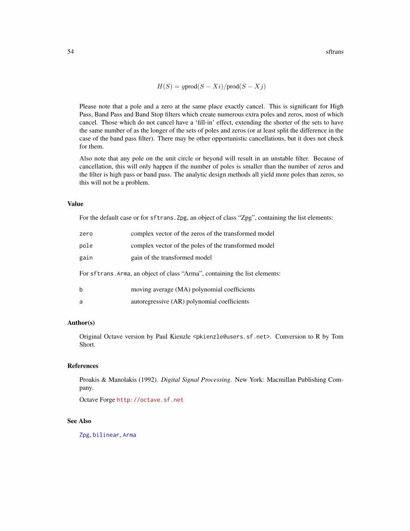
H(S) = gprod(S −Xi)/prod(S −Xj)

Please note that a pole and a zero at the same place exactly cancel. This is significant for HighPass, Band Pass and Band Stop filters which create numerous extra poles and zeros, most of whichcancel. Those which do not cancel have a ‘fill-in’ effect, extending the shorter of the sets to havethe same number of as the longer of the sets of poles and zeros (or at least split the difference in thecase of the band pass filter). There may be other opportunistic cancellations, but it does not checkfor them.

Also note that any pole on the unit circle or beyond will result in an unstable filter. Because ofcancellation, this will only happen if the number of poles is smaller than the number of zeros andthe filter is high pass or band pass. The analytic design methods all yield more poles than zeros, sothis will not be a problem.

Value

For the default case or for sftrans.Zpg, an object of class “Zpg”, containing the list elements:

zero complex vector of the zeros of the transformed model

pole complex vector of the poles of the transformed model

gain gain of the transformed model

For sftrans.Arma, an object of class “Arma”, containing the list elements:



Author(s)


References



See Also

Zpg, bilinear, Arma


sgolay 55

sgolay Savitzky-Golay smoothing filters

Description

Computes the filter coefficients for all Savitzky-Golay smoothing filters.

Usage

sgolay(p, n, m = 0, ts = 1)

Arguments

p filter order.

n filter length (must be odd).

m return the m-th derivative of the filter coefficients.

ts time scaling factor.

Details

The early rows of the result F smooth based on future values and later rows smooth based onpast values, with the middle row using half future and half past. In particular, you can use row ito estimate x[k] based on the i-1 preceding values and the n-i following values of x values asy[k] = F[i,] * x[(k-i+1):(k+n-i)].

Normally, you would apply the first (n-1)/2 rows to the first k points of the vector, the last k rowsto the last k points of the vector and middle row to the remainder, but for example if you wererunning on a realtime system where you wanted to smooth based on the all the data collected upto the current time, with a lag of five samples, you could apply just the filter on row n-5 to yourwindow of length n each time you added a new sample.

Value

An square matrix with dimensions length(n) that is of class 'sgolayFilter' (so it can be usedwith filter).

Author(s)

Original Octave version by Paul Kienzle <[email protected]>. Modified by Pascal Dupuis.Conversion to R by Tom Short.

References

William H. Press, Saul A. Teukolsky, William T. Vetterling, Brian P. Flannery, Numerical Recipesin C: The Art of Scientific Computing , 2nd edition, Cambridge Univ. Press, N.Y., 1992.



56 sgolayfilt

See Also

sgolayfilt, filter

sgolayfilt Apply a Savitzky-Golay smoothing filter

Description

Smooth data with a Savitzky-Golay smoothing filter.

Usage

sgolayfilt(x, p = 3, n = p + 3 - p%%2, m = 0, ts = 1)

## S3 method for class 'sgolayFilter'filter(filt, x, ...)

Arguments


p filter order.

n filter length (must be odd).

m return the m-th derivative of the filter coefficients.

ts time scaling factor.

filt filter characteristics (normally generated by sgolay).


Details

These filters are particularly good at preserving lineshape while removing high frequency squiggles.

Value

The filtered signal, of length(x).

Author(s)

Original Octave version by Paul Kienzle <[email protected]>. Modified by Pascal Dupuis.Conversion to R by Tom Short.

References



signal-internal 57

See Also

sgolay, filter

Examples

# Compare a 5 sample averager, an order-5 butterworth lowpass# filter (cutoff 1/3) and sgolayfilt(x, 3, 5), the best cubic# estimated from 5 points.bf <- butter(5,1/3)x <- c(rep(0,15), rep(10, 10), rep(0, 15))sg <- sgolayfilt(x)plot(sg, type="l")lines(filtfilt(rep(1, 5)/5,1,x), col = "red") # averaging filterlines(filtfilt(bf,x), col = "blue") # butterworthpoints(x, pch = "x") # original data

signal-internal Internal or uncommented functions

Description

Internal or barely commented functions not exported from the Namespace.

Details

# MOSTLY MATLAB/OCTAVE COMPATIBLE UTILITIESfractdiff(x, d) # Fractional differencespostpad(x, n) # pad \code{x} with zeros at the end for a total length \code{n}

# truncates if length(x) < nsinc(x) # sin(pi * x) / (pi * x)

# MATLAB-INCOMPATIBLE UTILITIESlogseq(from, to, n = 500) # like \code{linspace} but equally spaced logarithmically

# MAINLY INTERNAL, BUT MATLAB COMPATIBLEmkpp(x, P, d = round(NROW(P)/pp$n)) # used by \code{pchip}## Construct a piece-wise polynomial structure from sample points x and## coefficients P.ppval(pp, xi) # used by \code{pchip}## Evaluate piece-wise polynomial pp and points xi.ncauer(Rp, Rs, n) # used by \code{ellip}ellipke(m, Nmax) # used by \code{ellip}cheb(n, x) # nth-order Chebyshev polynomial calculated at x

# used by \code{chebwin}

58 specgram

specgram Spectrogram plot

Description

Generate a spectrogram for the signal. This chops the signal into overlapping slices, windows eachslice and applies a Fourier transform to determine the frequency components at that slice.

Usage

specgram(x, n = min(256, length(x)), Fs = 2, window = hanning(n),overlap = ceiling(length(window)/2))

## S3 method for class 'specgram'plot(x, col = gray(0:512 / 512), xlab="time", ylab="frequency", ...)

## S3 method for class 'specgram'print(x, col = gray(0:512 / 512), xlab="time", ylab="frequency", ...)

Arguments

x the vector of samples.

n the size of the Fourier transform window.

Fs the sample rate, Hz.

window shape of the fourier transform window, defaults to hanning(n). The windowlength for a hanning window can be specified instead.

overlap overlap with previous window, defaults to half the window length.

col color scale used for the underlying image function.

xlab,ylab axis labels with sensible defaults.

... additional arguments passed to the underlying plot functions.

Details

When results of specgram are printed, a spectrogram will be plotted. As with lattice plots,automatic printing does not work inside loops and function calls, so explicit calls to print or plotare needed there.

The choice of window defines the time-frequency resolution. In speech for example, a wide windowshows more harmonic detail while a narrow window averages over the harmonic detail and showsmore formant structure. The shape of the window is not so critical so long as it goes gradually tozero on the ends.

Step size (which is window length minus overlap) controls the horizontal scale of the spectrogram.Decrease it to stretch, or increase it to compress. Increasing step size will reduce time resolution,but decreasing it will not improve it much beyond the limits imposed by the window size (you dogain a little bit, depending on the shape of your window, as the peak of the window slides overpeaks in the signal energy). The range 1-5 msec is good for speech.

specgram 59

FFT length controls the vertical scale. Selecting an FFT length greater than the window lengthdoes not add any information to the spectrum, but it is a good way to interpolate between frequencypoints which can make for prettier spectrograms.

After you have generated the spectral slices, there are a number of decisions for displaying them.First the phase information is discarded and the energy normalized:

S = abs(S); S = S/max(S)

Then the dynamic range of the signal is chosen. Since information in speech is well above thenoise floor, it makes sense to eliminate any dynamic range at the bottom end. This is done bytaking the max of the magnitude and some minimum energy such as minE=-40dB. Similarly, thereis not much information in the very top of the range, so clipping to a maximum energy such asmaxE=-3dB makes sense:

S = max(S, 10^(minE/10)); S = min(S, 10^(maxE/10))

The frequency range of the FFT is from 0 to the Nyquist frequency of one half the sampling rate.If the signal of interest is band limited, you do not need to display the entire frequency range. Inspeech for example, most of the signal is below 4 kHz, so there is no reason to display up to theNyquist frequency of 10 kHz for a 20 kHz sampling rate. In this case you will want to keep onlythe first 40% of the rows of the returned S and f. More generally, to display the frequency range[minF, maxF], you could use the following row index:

idx = (f >= minF & f <= maxF)

Then there is the choice of colormap. A brightness varying colormap such as copper or bonegives good shape to the ridges and valleys. A hue varying colormap such as jet or hsv gives anindication of the steepness of the slopes. The final spectrogram is displayed in log energy scale andby convention has low frequencies on the bottom of the image.

Value

For specgram list of class specgram with items:

S complex output of the FFT, one row per slice.

f the frequency indices corresponding to the rows of S.

t the time indices corresponding to the columns of S.

Author(s)


References


See Also

fft, image


60 spencer

Examples

specgram(chirp(seq(-2, 15, by = 0.001), 400, 10, 100, 'quadratic'))specgram(chirp(seq(0, 5, by = 1/8000), 200, 2, 500, "logarithmic"), Fs = 8000)

data(wav) # contains wav$rate, wav$soundFs <- wav$ratestep <- trunc(5*Fs/1000) # one spectral slice every 5 mswindow <- trunc(40*Fs/1000) # 40 ms data windowfftn <- 2^ceiling(log2(abs(window))) # next highest power of 2spg <- specgram(wav$sound, fftn, Fs, window, window-step)S <- abs(spg$S[2:(fftn*4000/Fs),]) # magnitude in range 0<f<=4000 Hz.S <- S/max(S) # normalize magnitude so that max is 0 dB.S[S < 10^(-40/10)] <- 10^(-40/10) # clip below -40 dB.S[S > 10^(-3/10)] <- 10^(-3/10) # clip above -3 dB.image(t(20*log10(S)), axes = FALSE) #, col = gray(0:255 / 255))

spencer Spencer filter

Description

Spencer’s 15-point moving average filter.

Usage

spencer(x)

spencerFilter()

Arguments


Value

For spencer, the filtered signal. For spencerFilter, a vector of filter coefficients with class Mathat can be passed to filter.

Author(s)

Original Octave version by Friedrich Leisch. Conversion to R by Tom Short.

References


See Also

filter, Ma


unwrap 61

unwrap Unwrap radian phases

Description

Unwrap radian phases by adding multiples of 2*pi as appropriate to remove jumps.

Usage

unwrap(a, tol = pi, dim = 1)

Arguments

a vector of phase angles in radians.

tol tolerance for removing phase jumps.

dim dimension with which to apply the phase unwrapping.

Value

A vector with the unwrapped phase angles.

Author(s)

Original Octave version by Bill Lash. Conversion to R by Tom Short.

References


Examples

phase <- c(seq(0, 2*pi, length=500), seq(0, 2*pi, length=500))plot(phase, type = "l", ylim = c(0, 4*pi))lines(unwrap(phase), col = "blue")

wav Example wav file

Description

Example wav file audio waveshape from Octave.

Usage

data(wav)


62 Windowing functions

Format

The format is: List of 3 $ sound: num [1, 1:17380] -0.000275 -0.00061 -0.000397 -0.000793 -0.000305 ... $ rate : int 22050 $ bits : int 16 - attr(*, "class")= chr "Sample"

Details

Sound samples are in Element “sound” while “rate” is the sampling rate (in Hz) and “bits” theresolution of the underlying Wave file.

Source

Octave

Examples

data(wav)str(wav)

Windowing functions Windowing functions

Description

A variety of generally Matlab/Octave compatible filter generation functions, including Bartlett,Blackman, Hamming, Hanning, and triangular.

Usage

bartlett(n)blackman(n)boxcar(n)flattopwin(n, sym = c('symmetric', 'periodic'))gausswin(n, w = 2.5)hamming(n)hanning(n)triang(n)

Arguments

n length of the filter; number of coefficients to generate.

w the reciprocal of the standard deviation for gausswin. Use larger a for a nar-rower window.

sym 'symmetric' for a symmetric window, 'periodic' for a periodic window.

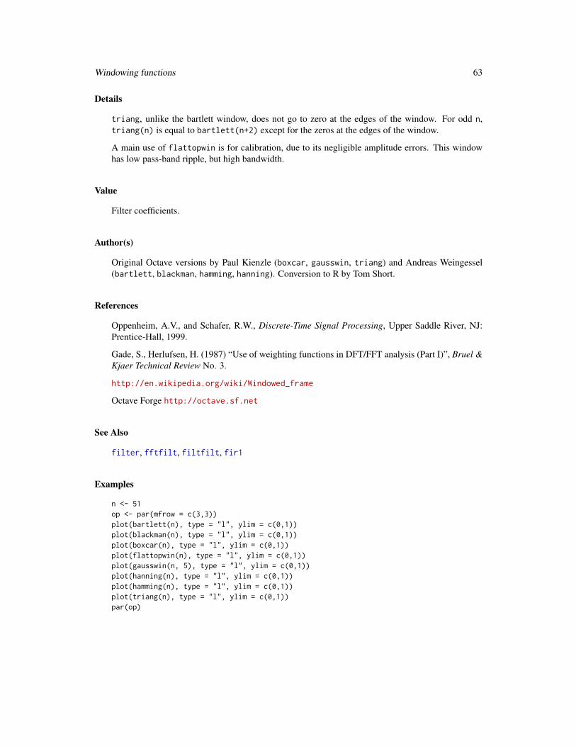
Windowing functions 63

Details

triang, unlike the bartlett window, does not go to zero at the edges of the window. For odd n,triang(n) is equal to bartlett(n+2) except for the zeros at the edges of the window.

A main use of flattopwin is for calibration, due to its negligible amplitude errors. This windowhas low pass-band ripple, but high bandwidth.

Value

Filter coefficients.

Author(s)

Original Octave versions by Paul Kienzle (boxcar, gausswin, triang) and Andreas Weingessel(bartlett, blackman, hamming, hanning). Conversion to R by Tom Short.

References

Oppenheim, A.V., and Schafer, R.W., Discrete-Time Signal Processing, Upper Saddle River, NJ:Prentice-Hall, 1999.

Gade, S., Herlufsen, H. (1987) “Use of weighting functions in DFT/FFT analysis (Part I)”, Bruel &Kjaer Technical Review No. 3.

http://en.wikipedia.org/wiki/Windowed_frame


See Also

filter, fftfilt, filtfilt, fir1

Examples

n <- 51op <- par(mfrow = c(3,3))plot(bartlett(n), type = "l", ylim = c(0,1))plot(blackman(n), type = "l", ylim = c(0,1))plot(boxcar(n), type = "l", ylim = c(0,1))plot(flattopwin(n), type = "l", ylim = c(0,1))plot(gausswin(n, 5), type = "l", ylim = c(0,1))plot(hanning(n), type = "l", ylim = c(0,1))plot(hamming(n), type = "l", ylim = c(0,1))plot(triang(n), type = "l", ylim = c(0,1))par(op)

http://en.wikipedia.org/wiki/Windowed_frame


64 Zpg

Zpg Zero-pole-gain model

Description

Zero-pole-gain model of an ARMA filter.

Usage

Zpg(zero, pole, gain)

## S3 method for class 'Arma'as.Zpg(x, ...)

## S3 method for class 'Ma'as.Zpg(x, ...)

## S3 method for class 'Zpg'as.Zpg(x, ...)

Arguments

zero complex vector of the zeros of the model.pole complex vector of the poles of the model.gain gain of the model.x model to be converted.... additional arguments (ignored).

Details

as.Zpg converts from other forms, including Arma and Ma.

Value

An object of class “Zpg”, containing the list elements:

zero complex vector of the zeros of the model.pole complex vector of the poles of the model.gain gain of the model.

Author(s)

Tom Short

See Also

Arma, bilinear

zplane 65

zplane Pole-zero plot

Description

Plot the poles and zeros of a model or filter.

Usage

## Default S3 method:zplane(filt, a, ...)

## S3 method for class 'Arma'zplane(filt, ...)

## S3 method for class 'Ma'zplane(filt, ...)

## S3 method for class 'Zpg'zplane(filt, ...)

Arguments



... Additional arguments passed to plot.

Details

Poles are marked with an ‘x’, and zeros are marked with an ‘o’.

Value

No value is returned.

Author(s)

Tom Short

References


http://en.wikipedia.org/wiki/Pole-zero_plot


http://en.wikipedia.org/wiki/Pole-zero_plot

66 zplane

See Also

Arma, freqz

Examples

filt <- ellip(5, 0.5, 20, .2)zplane(filt)

Index

∗Topic datasetswav, 61

∗Topic mathan, 4Arma, 5bilinear, 6butter, 8buttord, 10cheb1ord, 11chebwin, 12cheby1, 14chirp, 16conv, 17decimate, 18ellip, 19ellipord, 21fftfilt, 22filter, 23FilterOfOrder, 25filtfilt, 26fir1, 27fir2, 28freqs, 29freqz, 31grpdelay, 33ifft, 35impz, 36interp, 37interp1, 38kaiser, 40kaiserord, 41levinson, 43Ma, 44medfilt1, 44pchip, 46poly, 47polyval, 48remez, 48resample, 49

roots, 51sftrans, 52sgolay, 55sgolayfilt, 56signal-internal, 57specgram, 58spencer, 60unwrap, 61Windowing functions, 62Zpg, 64zplane, 65

∗Topic packagesignal-package, 3

an, 4approx, 39, 47Arma, 5, 8, 9, 15, 20, 22, 24, 27, 31, 32, 34, 44,

54, 64, 66as.Arma (Arma), 5as.Zpg, 6as.Zpg (Zpg), 64

bartlett (Windowing functions), 62bilinear, 6, 54, 64blackman (Windowing functions), 62boxcar (Windowing functions), 62butter, 6, 8, 11, 15, 20, 22, 25buttord, 9, 10, 12, 25

cheb (signal-internal), 57cheb1ord, 11, 11, 15, 25chebwin, 12cheby1, 6, 9, 12, 14, 20, 22, 25cheby2 (cheby1), 14chirp, 16conv, 17, 47, 51convolve, 18

decimate, 18, 38, 50

ellip, 9, 15, 19, 25

67

68 INDEX

ellipke (signal-internal), 57ellipord, 20, 21, 22, 25

fft, 18, 23, 35, 59fftfilt, 18, 22, 24, 27–29, 49, 63FftFilter (fftfilt), 22filter, 6, 9, 15, 19, 20, 22, 23, 23, 24, 25,

27–29, 31, 32, 34, 37, 39, 45, 49, 50,56, 57, 60, 63

filter.FftFilter (fftfilt), 22filter.MedianFilter (medfilt1), 44filter.sgolayFilter (sgolayfilt), 56FilterOfOrder, 11, 12, 25filtfilt, 18, 23, 24, 26, 63fir1, 27, 29, 38, 49, 63fir2, 28, 28flattopwin (Windowing functions), 62fractdiff (signal-internal), 57freqs, 29, 32freqs_plot (freqs), 29freqz, 31, 31, 34, 37, 66freqz_plot (freqz), 31

gausswin (Windowing functions), 62grpdelay, 33

hamming, 40, 42hamming (Windowing functions), 62hanning (Windowing functions), 62

ifft, 18, 35image, 58, 59impz, 36interp, 19, 37, 39, 50interp1, 38, 38, 47

kaiser, 13, 40, 42kaiserord, 40, 41

levinson, 43logseq (signal-internal), 57

Ma, 6, 23, 28, 29, 44, 49, 60matlab, 4medfilt1, 44median, 45MedianFilter (medfilt1), 44mkpp (signal-internal), 57

ncauer (signal-internal), 57

pchip, 46plot, 33, 36plot.freqs (freqs), 29plot.freqz (freqz), 31plot.grpdelay (grpdelay), 33plot.impz (impz), 36plot.specgram (specgram), 58poly, 18, 47, 48, 51polyroot, 51polyval, 47, 48, 51postpad (signal-internal), 57ppval (signal-internal), 57print.freqs (freqs), 29print.freqz (freqz), 31print.grpdelay (grpdelay), 33print.impz (impz), 36print.specgram (specgram), 58

remez, 48resample, 19, 38, 39, 49roots, 47, 48, 51runmed, 24, 45

sftrans, 8, 52sgolay, 55, 57sgolayfilt, 56, 56signal (signal-package), 3signal-internal, 57signal-package, 3sinc (signal-internal), 57specgram, 17, 58spencer, 60spencerFilter (spencer), 60spline, 39, 47

triang (Windowing functions), 62

unwrap, 61

wav, 61Windowing functions, 62

Zpg, 8, 54, 64zplane, 37, 65

package 'signal

Documents