package ‘distatisr’ - the comprehensive r archive network · package ‘distatisr ... valentin,...

Package ‘DistatisR’February 19, 2015

Type Package

Title DiSTATIS Three Way Metric Multidimensional Scaling

Version 1.0

Date 2013-07-10

Author Derek Beaton [aut, com, ctb], Cherise Chin Fatt [ctb], Herve Abdi [aut, cre]

Maintainer Derek Beaton <[email protected]>

DescriptionImplement DiSTATIS and CovSTATIS (three-way multidimensional scaling). For the analy-sis of multiple distance/covariance matrices collected on the same set of observations

License GPL-2

Depends prettyGraphs (>= 2.0.0), car

URL www.utdallas.edu/~herve

NeedsCompilation no

Repository CRAN

Date/Publication 2013-07-11 07:24:31

R topics documented:DistatisR-package . . . . . . . . . . . . . . . . . . . . . . . . . . . . . . . . . . . . . . 2BootFactorScores . . . . . . . . . . . . . . . . . . . . . . . . . . . . . . . . . . . . . . 5BootFromCompromise . . . . . . . . . . . . . . . . . . . . . . . . . . . . . . . . . . . 7Chi2Dist . . . . . . . . . . . . . . . . . . . . . . . . . . . . . . . . . . . . . . . . . . . 9Chi2DistanceFromSort . . . . . . . . . . . . . . . . . . . . . . . . . . . . . . . . . . . 11DistAlgo . . . . . . . . . . . . . . . . . . . . . . . . . . . . . . . . . . . . . . . . . . . 13DistanceFromSort . . . . . . . . . . . . . . . . . . . . . . . . . . . . . . . . . . . . . . 13distatis . . . . . . . . . . . . . . . . . . . . . . . . . . . . . . . . . . . . . . . . . . . . 15GraphDistatisAll . . . . . . . . . . . . . . . . . . . . . . . . . . . . . . . . . . . . . . 18GraphDistatisBoot . . . . . . . . . . . . . . . . . . . . . . . . . . . . . . . . . . . . . 20GraphDistatisCompromise . . . . . . . . . . . . . . . . . . . . . . . . . . . . . . . . . 22GraphDistatisPartial . . . . . . . . . . . . . . . . . . . . . . . . . . . . . . . . . . . . . 24GraphDistatisRv . . . . . . . . . . . . . . . . . . . . . . . . . . . . . . . . . . . . . . 25mmds . . . . . . . . . . . . . . . . . . . . . . . . . . . . . . . . . . . . . . . . . . . . 27

1

2 DistatisR-package

print.Cmat . . . . . . . . . . . . . . . . . . . . . . . . . . . . . . . . . . . . . . . . . . 29print.DistatisR . . . . . . . . . . . . . . . . . . . . . . . . . . . . . . . . . . . . . . . . 30print.Splus . . . . . . . . . . . . . . . . . . . . . . . . . . . . . . . . . . . . . . . . . . 30SortingBeer . . . . . . . . . . . . . . . . . . . . . . . . . . . . . . . . . . . . . . . . . 31SortingSpice . . . . . . . . . . . . . . . . . . . . . . . . . . . . . . . . . . . . . . . . . 31

Index 33

DistatisR-package DistatisR: DISTATIS Three Way Metric Multidimensional Scaling

Description

DistatisR package implements three way multidimensional scaling: DISTATIS and COVSTATIS.

Analyses sets of distance (or covariance) matrices collected on the same set of observations

Details

Package: DistatisRType: PackageVersion: 1.0Date: 2013-07-03License: GPL-2Depends: prettyGraphs (>= 2.0.0), car

The example shown here comes from Abdi et al. (2007), distatis paper on the sorting task.

Author(s)

Derek Beaton [aut, com, ctb], Cherise Chin Fatt [ctb], & Herve Abdi [aut, cre]

Maintainer: Derek Beaton <[email protected]>

References

Note: these papers are available from www.utdallas.edu/~herve

Abdi, H., Valentin, D., O’Toole, A.J., & Edelman, B. (2005). DISTATIS: The analysis of multi-ple distance matrices. Proceedings of the IEEE Computer Society: International Conference onComputer Vision and Pattern Recognition. (San Diego, CA, USA). pp. 42-47.

Abdi, H., Valentin, D., Chollet, S., & Chrea, C. (2007). Analyzing assessors and products in sortingtasks: DISTATIS, theory and applications. Food Quality and Preference, 18, 627–640.

Abdi, H., & Valentin, D., (2007). Some new and easy ways to describe, compare, and evaluateproducts and assessors. In D., Valentin, D.Z. Nguyen, L. Pelletier (Eds): New trends in sensoryevaluation of food and non-food products. Ho Chi Minh (Vietnam): Vietnam National University& Ho Chi Minh City Publishing House. pp. 5–18.

www.utdallas.edu/~herve

DistatisR-package 3

Abdi, H., Dunlop, J.P., & Williams, L.J. (2009). How to compute reliability estimates and displayconfidence and tolerance intervals for pattern classiffers using the Bootstrap and 3-way multidimen-sional scaling (DISTATIS). NeuroImage, 45, 89–95.

Abdi, H., Williams, L.J., Valentin, D., & Bennani-Dosse, M. (2012). STATIS and DISTATIS:Optimum multi-table principal component analysis and three way metric multidimensional scaling.Wiley Interdisciplinary Reviews: Computational Statistics, 4, 124–167.

Chollet, S., Valentin, D., & Abdi, H. (in press, 2013). The free sorting task. In. P.V. Tomasco & G.Ares (Eds), Novel Techniques in Sensory Characterization and Consumer Profiling. Boca Raton:Taylor and Francis.

Valentin, D., Chollet, S., Nestrud, M., & Abdi, H. (in press, 2013). Sorting and similarity method-ologies. In. S. Kemp, S., J. Hort, & T. Hollowood (Eds.), Descriptive Analysis in Sensory Evalua-tion. London: Wiley-Blackwell.

See Also

distatis BootFactorScores BootFromCompromise DistanceFromSort distatis GraphDistatisAllGraphDistatisBoot GraphDistatisCompromise GraphDistatisPartial GraphDistatisRv mmdsprettyGraphs

Examples

# Here we use the sorting task from Abdi et al, 2007 paper.# where 10 Assessors sorted 8 beers

#-----------------------------------------------------------------------------# 1. Get the data from the 2007 sorting example# this is the way they look from Table 1 of# Abdi et al. (2007).# Assessors# 1 2 3 4 5 6 7 8 9 10# Beer Sex f m f f m m m m f m# -----------------------------#Affligen 1 4 3 4 1 1 2 2 1 3#Budweiser 4 5 2 5 2 3 1 1 4 3#Buckler_Blonde 3 1 2 3 2 4 3 1 1 2#Killian 4 2 3 3 1 1 1 2 1 4#St. Landelin 1 5 3 5 2 1 1 2 1 3#Buckler_Highland 2 3 1 1 3 5 4 4 3 1#Fruit Defendu 1 4 3 4 1 1 2 2 2 4#EKU28 5 2 4 2 4 2 5 3 4 5

# 1.1. Create the# Name of the BeersBeerName <- c('Affligen', 'Budweiser','Buckler Blonde',

'Killian','St.Landelin','Buckler Highland','Fruit Defendu','EKU28')

# 1.2. Create the name of the Assessors# (F are females, M are males)Juges <- c('F1','M2', 'F3', 'F4', 'M5', 'M6', 'M7', 'M8', 'F9', 'M10')

4 DistatisR-package

# 1.3. Get the sorting dataSortData <- c(1, 4, 3, 4, 1, 1, 2, 2, 1, 3,

4, 5, 2, 5, 2, 3, 1, 1, 4, 3,3, 1, 2, 3, 2, 4, 3, 1, 1, 2,4, 2, 3, 3, 1, 1, 1, 2, 1, 4,1, 5, 3, 5, 2, 1, 1, 2, 1, 3,2, 3, 1, 1, 3, 5, 4, 4, 3, 1,1, 4, 3, 4, 1, 1, 2, 2, 2, 4,5, 2, 4, 2, 4, 2, 5, 3, 4, 5)

# 1.4 Create a data frameSort <- matrix(SortData,ncol = 10, byrow= TRUE, dimnames = list(BeerName, Juges))# (alternatively we could have read a csv file)# 1.5 Example of how to read a csv filw# Sort <- read.table("BeeerSortingTask.csv", header=TRUE,# sep=",", na.strings="NA", dec=".", row.names=1, strip.white=TRUE)

#-----------------------------------------------------------------------------# 2. Create the set of distance matrices (one distance matrix per assessor)# (uses the function DistanceFromSort)DistanceCube <- DistanceFromSort(Sort)#-----------------------------------------------------------------------------# 3. Call the DISTATIS routine with the cube of distance as parametertestDistatis <- distatis(DistanceCube)# The factor scores for the beers are in# testDistatis$res4Splus$F# the factor scores for the assessors are in (RV matrice)# testDistatis$res4Cmat$G

#-----------------------------------------------------------------------------# 4. Inferences on the beers obtained via bootstrap# here we use two different bootstraps:# 1. Bootstrap on factors (very fast but could be too liberal# when the number of assessors is very large)# 2. Complete bootstrap obtained by computing sets of compromises# and projecting them (could be significantly longer because a lot# of computations is required)## 4.1 Get the bootstrap factor scores (with default 1000 iterations)BootF <- BootFactorScores(testDistatis$res4Splus$PartialF)## 4.2 Get the boostrap from full bootstrap (default niter = 1000)F_fullBoot <- BootFromCompromise(DistanceCube,niter=1000)

#-----------------------------------------------------------------------------# 5. Create the Graphics# 5.1 an Rv maprv.graph.out <- GraphDistatisRv(testDistatis$res4Cmat$G)

# 5.2 a compromise plotcompromise.graph.out <- GraphDistatisCompromise(testDistatis$res4Splus$F)

# 5.3 a partial factor score plotpartial.scores.graph.out <-

BootFactorScores 5

GraphDistatisPartial(testDistatis$res4Splus$F,testDistatis$res4Splus$PartialF)# 5.4 a bootstrap confidence interval plot#5.4.1 with ellipsesboot.graph.out.ell <- GraphDistatisBoot(testDistatis$res4Splus$F,BootF)#or# boot.graph.out <- GraphDistatisBoot(testDistatis$res4Splus$F,F_fullBoot)#5.4.2 with hullsboot.graph.out.hull <- GraphDistatisBoot(testDistatis$res4Splus$F,BootF,ellipses=FALSE)#or# boot.graph.out <- GraphDistatisBoot(testDistatis$res4Splus$F,F_fullBoot,ellipses=FALSE)#5.5 all the plots at onceall.plots.out <-GraphDistatisAll(testDistatis$res4Splus$F,testDistatis$res4Splus$PartialF,BootF,testDistatis$res4Cmat$G)

BootFactorScores BootFactorSCores Compute observation Bootstrap replicates of thefactor scores from partial factor scores

Description

BootFactorSCores Compute Bootstrap replicates of the factor scores of the observations frompartial factor scores. The input is obtained from the distatis function, the output is a 3-way arrayof dimensions number of observations by number of factors by number of replicates. The outputis typically used to plot confidence intervals (i.e., ellipsoids or convex hulls) or to compute t-likestatistic called bootstrap ratios.

Usage

BootFactorScores(PartialFS, niter = 1000)

Arguments

PartialFS The partial factor scores (e.g., obtaiined from distatis)niter number of boostrap iterations (default = 1000)

Details

To compute a bootstrapped sample a set of K distance matrices is selected with replacement fromthe original set of K distance matrices. The partial factors scores of the selected distance matricesare then averaged to produce the bootstrapped estimate of the factor scores of the observations.This approach is also called partial boostrap by Lebart (2007, see also Chateau & Lebart 1996). Ithas the advantage of being very fast even for very large data sets Recent work (Cadoret & Husson,2012), however, suggests that partial boostrap could lead to optimistic bootstrap estimates when thenumber of distance matrices is large and that it is preferable to use instead a total boostrap approach(i.e., creating new compromises by resampling and then projecting them on the common solutionsee function BootFromCompromise, and Cadoret & Husson, 2012 see also Abdi et al., 2009 for anexample).

6 BootFactorScores

Value

the output is a 3-way array of dimensions "number of observations by number of factors by numberof replicates."

Author(s)

Herve Abdi

References

Abdi, H., & Valentin, D., (2007). Some new and easy ways to describe, compare, and evaluateproducts and assessors. In D., Valentin, D.Z. Nguyen, L. Pelletier (Eds) New trends in sensoryevaluation of food and non-food products. Ho Chi Minh (Vietnam): Vietnam National University-Ho chi Minh City Publishing House. pp. 5-18.



These papers are available from www.utdallas.edu/~herve

Additional references:

Cadoret, M., Husson, F. (2012) Construction and evaluation of confidence ellipses applied at sen-sory data. Food Quality and Preference, 28, 106–115.

Chateau, F., & Lebart, L. (1996). Assessing sample variability in the visualization techniques re-lated to principal component analysis: Bootstrap and alternative simulation methods. In A. Prats(Ed.),Proceedings of COMPSTAT 2006. Heidelberg: Physica Verlag.

Lebart, L. (2007). Which bootstrap for principal axes methods? In Selected contributions in dataanalysis and classification, COMPSTAT 2006. Heidelberg: Springer Verlag.

See Also

BootFromCompromise GraphDistatisBoot

Examples

# 1. Load the Sort data set from the SortingBeer example (available from the DistatisR package)data(SortingBeer)# Provide an 8 beers by 10 assessors set of results of a sorting task#-----------------------------------------------------------------------------# 2. Create the set of distance matrices (one distance matrix per assessor)# (ues the function DistanceFromSort)DistanceCube <- DistanceFromSort(Sort)

#-----------------------------------------------------------------------------# 3. Call the DISTATIS routine with the cube of distance as parameter


BootFromCompromise 7

testDistatis <- distatis(DistanceCube)# The factor scores for the beers are in# testDistatis$res4Splus$F# the partial factor score for the beers for the assessors are in# testDistatis$res4Splus$PartialF## 4. Get the bootstraped factor scores (with default 1000 iterations)BootF <- BootFactorScores(testDistatis$res4Splus$PartialF)

BootFromCompromise Compute observation Bootstrap replicates of the factor scores frombootstrapped compromises

Description

BootFactorSCores computes Bootstrap replicates of the factor scores of the observations frombootstrapped compromises. The input is obtained from the same input as the distatis function,the output is a 3-way array of dimensions "number of observations by number of factors by numberof replicates." The output is typically used to plot confidence intervals (i.e., ellipsoids or convexhulls) or to compute t-like statistic called bootstrap ratios.

Usage

BootFromCompromise(LeCube2Distance,niter = 1000, Norm = "MFA",Distance = TRUE, RV = TRUE,nfact2keep = 3)

Arguments

LeCube2Distance

The array of distance used to call distatis

niter The number of bootstrap iterations (default = 1000)

Norm should be the same as for the original call to distatis

Distance should be the same as for the original call to distatis

RV should be the same as for the original call to distatis

nfact2keep number of factors to keep for the results

Details

To compute a bootstrapped sample a set of K distance matrices is selected with replacement fromthe original set of K distance matrices. A distatis compromise is then computed and projectedon the factor space of the original solution to obtain the bootstrapped factor scores. This approachis also called total boostrap by Lebart (2007, see also Chateau and Lebart 1996, see also Abdi et al.,2009 for an example). Compared to the partial bootstrap (see help for BootFactorScores) It has thedesadvantage of being slow espcially for large data sets but recent work (Cadoret & Husson, 2012)

8 BootFromCompromise

suggests that partial boostrap (i.e., computed from the partial factor scores) could lead to optimisticbootstrap estimates when the number of distance matrices is large and that it is preferable to useinstead the total boostrap.

Value

the output is a 3-way array of dimensions "number of observations by number of factors by numberof replicates."

Author(s)

Herve Abdi

References

Abdi, H., & Valentin, D., (2007). Some new and easy ways to describe, compare, and evaluateproducts and assessors. In D., Valentin, D.Z. Nguyen, L. Pelletier (Eds) New trends in sensoryevaluation of food and non-food products. Ho Chi Minh (Vietnam): Vietnam National University-Ho chi Minh City Publishing House. pp. 5-18.




Additional references:

Cadoret, M., Husson, F. (2012) Construction and evaluation of confidence ellipses applied at sen-sory data. Food Quality and Preference, 28, 106–115.

Chateau, F., & Lebart, L. (1996). Assessing sample variability in the visualization techniques re-lated to principal component analysis: Bootstrap and alternative simulation methods. In A. Prats(Ed.),Proceedings of COMPSTAT 2006. Heidelberg: Physica Verlag.

Lebart, L. (2007). Which bootstrap for principal axes methods? In Selected contributions in dataanalysis and classification, COMPSTAT 2006. Heidelberg: Springer Verlag.

See Also

BootFactorScores GraphDistatisBoot

Examples

# 1. Load the Sort data set from the SortingBeer example# (available from the DistatisR package)data(SortingBeer)# Provide the "8 beers by 10 assessors" results of a sorting task#-----------------------------------------------------------------------------


Chi2Dist 9

# 2. Create the set of distance matrices (one distance matrix per assessor)# (uses the function DistanceFromSort)DistanceCube <- DistanceFromSort(Sort)

#-----------------------------------------------------------------------------# 3. Call the distatis function with the cube of distance as parametertestDistatis <- distatis(DistanceCube)# The factor scores for the beers are in# testDistatis$res4Splus$F# the partial factor scores for the beers for the assessors are in# testDistatis$res4Splus$PartialF## 4. Get the bootstraped factor scores (with default 1000 iterations)# Here we use the "total bootstrap"F_fullBoot <- BootFromCompromise(DistanceCube,niter=1000)

Chi2Dist χˆ2 distance between the rows of a rectangular matrix.

Description

Computesthe I×I matrix D which is the χ2 distance matrix between the rows of an I×J rectangularmatrix X (with non-negative elements), and provides the I × 1 m vector of mass (where the massof a row is the sum of the entries of this row divided by the grand total of the matrix). When thedistance matrix and the associated vector of masses are used as input to the function mmds the resultswill give the factor scores of the correspondence analysis of the matrix X. The function is used bythe function Chi2DistanceFromSort that computes the χ2 distance for the results of a sorting task.

Usage

Chi2Dist(X)

Arguments

X A rectangle matrix with non-negative elements

Value

Sends back a list

$Distance the squared χ2 distance matrix computed the rows of matrix X.

masses the vector of masses of the rows of of matrix X.

Author(s)

Herve Abdi

10 Chi2Dist

References

The procedure and references are detailled in (Paper available from www.utdallas.edu/~herve):Abdi, H. (2007). Distance. In N.J. Salkind (Ed.): Encyclopedia of Measurement and Statistics.Thousand Oaks (CA): Sage. pp. 304–308.

And in:Abdi, H., & Valentin, D. (2006). Mathematiques pour les Sciences Cognitives (Mathematics forCognitive Sciences). Grenoble: PUG.

See also (for the example):

Abdi, H., & Williams, L.J. (2010). Principal component analysis. Wiley Interdisciplinary Reviews:Computational Statistics,2, 433–459.

See Also

Chi2DistanceFromSort distatis mmds

Examples

# Here is a data matrix from Abdi & Williams (2012)# page 449, Table 15. Punctuation of 6 French authorsPunctuation = matrix(c(

7836, 13112, 6026,53655, 102383, 42413,115615, 184541, 59226,161926, 340479, 62754,38177, 105101, 12670,46371, 58367, 14299),

ncol =3,byrow = TRUE)colnames(Punctuation) <-c('Period','Comma','Other')rownames(Punctuation) <-c('Rousseau','Chateaubriand',

'Hugo','Zola','Proust','Giroudoux')# 1. Get the Chi2 distance matrix# between the rows of PunctuationDres <- Chi2Dist(Punctuation)# check that the mds of the Chi2 distance matrix# with CA-masses gives the CA factor scores for I# 2. Use function mmds from DistatisR#testmds <- mmds(Dres$Distance,masses=Dres$masses)# Print the MDS factor scores from mmdsprint('Factor Scores from mds')print(testmds$FactorScores)print('It matches CA on X (see Abdi & Williams, 2010. Table 16, p. 449)')# Et voila!


Chi2DistanceFromSort 11

Chi2DistanceFromSort Creates a 3-dimensional χˆ2 distance array from the results of a sort-ing task.

Description

Takes the results from a (plain) sorting task where K assessors sort I observations into (mutuallyexclusive) groups (i.e., one object is in one an only one group). DistanceFromSort creates anI×I×K array of distance in which each of the k "slices" stores the (sorting) distance matrix of thekth assessor. In one of these distance matrices, the distance between rows is the χ2 distance betweenrows when the results of the task are coded as 0/1 group coding (i.e., the "complete disjunctivecoding" as used iin multiple correspondence analysis, see Abdi & Valentin, 2007, for more)

The ouput ot the function DistanceFromSort is used as input for the function distatis.

Usage

Chi2DistanceFromSort(X)

Arguments

X gives the results of a sorting task (see example below) as a objects (row) byassessors (columns) matrix.

Details

The input should have assessors as columns and observations as rows (see example below)

Value

DistanceFromSort returns a I × I ×K array of distances

Author(s)

Herve Abdi

References

See examples in


Abdi, H., & Valentin, D., (2007). Some new and easy ways to describe, compare, and evaluateproducts and assessors. In D., Valentin, D.Z. Nguyen, L. Pelletier (Eds) New trends in sensoryevaluation of food and non-food products. Ho Chi Minh (Vietnam): Vietnam National University-Ho chi Minh City Publishing House. pp. 5–18.

Abdi, H., & Valentin, D. (2007). Multiple correspondence analysis. In N.J. Salkind (Ed.): Encyclo-pedia of Measurement and Statistics. Thousand Oaks (CA): Sage. pp. 651-657.



12 Chi2DistanceFromSort

See Also

distatis

Examples

# 1. Get the data from the 2007 sorting example# this is the eay they look from Table 1 of# Abdi et al. (2007).# Assessors# 1 2 3 4 5 6 7 8 9 10# Beer Sex f m f f m m m m f m# -----------------------------#Affligen 1 4 3 4 1 1 2 2 1 3#Budweiser 4 5 2 5 2 3 1 1 4 3#Buckler_Blonde 3 1 2 3 2 4 3 1 1 2#Killian 4 2 3 3 1 1 1 2 1 4#St. Landelin 1 5 3 5 2 1 1 2 1 3#Buckler_Highland 2 3 1 1 3 5 4 4 3 1#Fruit Defendu 1 4 3 4 1 1 2 2 2 4#EKU28 5 2 4 2 4 2 5 3 4 5

## 1.1. Create the# Name of the BeersBeerName <- c('Affligen', 'Budweiser','Buckler Blonde',




4, 5, 2, 5, 2, 3, 1, 1, 4, 3,3, 1, 2, 3, 2, 4, 3, 1, 1, 2,4, 2, 3, 3, 1, 1, 1, 2, 1, 4,1, 5, 3, 5, 2, 1, 1, 2, 1, 3,2, 3, 1, 1, 3, 5, 4, 4, 3, 1,1, 4, 3, 4, 1, 1, 2, 2, 2, 4,5, 2, 4, 2, 4, 2, 5, 3, 4, 5)

# 1.4 Create a data frameSort <- matrix(SortData,ncol = 10, byrow= TRUE, dimnames = list(BeerName, Juges))##-----------------------------------------------------------------------------# 2. Create the set of distance matrices (one distance matrix per assessor)# (use the function DistanceFromSort)DistanceCube <- Chi2DistanceFromSort(Sort)#-----------------------------------------------------------------------------# 3. Call the DISTATIS routine with the cube of distance# obtained from DistanceFromSort as a parameter for the distatis functiontestDistatis <- distatis(DistanceCube)

DistAlgo 13

DistAlgo Four computer algorithms evaluate the similiarity of six faces for dis-tatis analysis

Description

Provide the data.frame DistAlgo Data set to be used to illustrated the use of the package DistatisR.Four algorithms evaluate the similarity (i.e., distance) between six faces (3 females and 3 males).Each algorithm provides a 6× 6 distance matrix evaluating the distance between each pair of faces.

Usage

data(DistAlgo)

Format

an 6× 6 array. Each 6× 6 matrix is a distance matrix

Source

Abdi et al. (2005). www.utdallas.edu/~herve

References

Abdi, H., Valentin, D., O’Toole, A.J., & Edelman, B. (2005). DISTATIS: The analysis of multi-ple distance matrices. Proceedings of the IEEE Computer Society: International Conference onComputer Vision and Pattern Recognition. (San Diego, CA, USA). pp. 42–47.

DistanceFromSort Creates a 3-dimensional distance array from the results of a sortingtask.

Description

Takes the results from a (plain) sorting task where K assessors sort I observations into (mutuallyexclusive) groups (i.e., one object is in one an only one group). DistanceFromSort creates anI × I ×K array of distance in which each of the k "slices" stores the (sorting) distance matrix ofthe kth assessor. In one of these distance matrices, a value of 0 at the intersection of a row and acolumn means that the object represented by the row and the object represented by the column weresorted together (i.e., they are a distance of 0), and a vaue of 1 means these two objects were put intodifferent groups.

The ouput ot the function DistanceFromSort is used as input for the function distatis.

Usage

DistanceFromSort(X)


14 DistanceFromSort

Arguments

X gives the results of a sorting task (see example below) as a objects (row) byassessors (columns) matrix.

Details

The input should have assessors as columns and observations as rows (see example below)

Value

DistanceFromSort returns a I × I ×K array of distances

Author(s)

Herve Abdi

References

See examples in




See Also

distatis

Examples

# 1. Get the data from the 2007 sorting example# this is the eay they look from Table 1 of# Abdi et al. (2007).# Assessors# 1 2 3 4 5 6 7 8 9 10# Beer Sex f m f f m m m m f m# -----------------------------#Affligen 1 4 3 4 1 1 2 2 1 3#Budweiser 4 5 2 5 2 3 1 1 4 3#Buckler_Blonde 3 1 2 3 2 4 3 1 1 2#Killian 4 2 3 3 1 1 1 2 1 4#St. Landelin 1 5 3 5 2 1 1 2 1 3#Buckler_Highland 2 3 1 1 3 5 4 4 3 1#Fruit Defendu 1 4 3 4 1 1 2 2 2 4#EKU28 5 2 4 2 4 2 5 3 4 5

#


distatis 15

# 1.1. Create the# Name of the BeersBeerName <- c('Affligen', 'Budweiser','Buckler Blonde',




4, 5, 2, 5, 2, 3, 1, 1, 4, 3,3, 1, 2, 3, 2, 4, 3, 1, 1, 2,4, 2, 3, 3, 1, 1, 1, 2, 1, 4,1, 5, 3, 5, 2, 1, 1, 2, 1, 3,2, 3, 1, 1, 3, 5, 4, 4, 3, 1,1, 4, 3, 4, 1, 1, 2, 2, 2, 4,5, 2, 4, 2, 4, 2, 5, 3, 4, 5)

# 1.4 Create a data frameSort <- matrix(SortData,ncol = 10, byrow= TRUE, dimnames = list(BeerName, Juges))##-----------------------------------------------------------------------------# 2. Create the set of distance matrices (one distance matrix per assessor)# (use the function DistanceFromSort)DistanceCube <- DistanceFromSort(Sort)#-----------------------------------------------------------------------------# 3. Call the DISTATIS routine with the cube of distance# obtained from DistanceFromSort as a parameter for the distatis functiontestDistatis <- distatis(DistanceCube)

distatis distatis 3-Way MDS based on the STATIS optimization procedure

Description

Implements the DISTATIS method which a 3-way generalization of metric multidimensional scaling(a.k.a. classical MDS or principal coordinate analysis). distatis takes a set ofK distance matricesdescribing a set of I observations and computes (1) a set of factor scores that describes the similaritystructure of the distance matrices (e.g., what distance matrices describe the observations in the sameway, what distance matrices differ from each other) (2) a set of factor scores (called the compromisefactor scores) for the observations that best describes the similarity structure of the observationsand (3) partial factor scores that show how each individual distance matrix "sees" the compromisespace. distatis computes the compromise as an optimum linear combination of the cross-productmatrices associated to each distance matrix. distatis can also be applied to a set of covariancematrices.

16 distatis

Usage

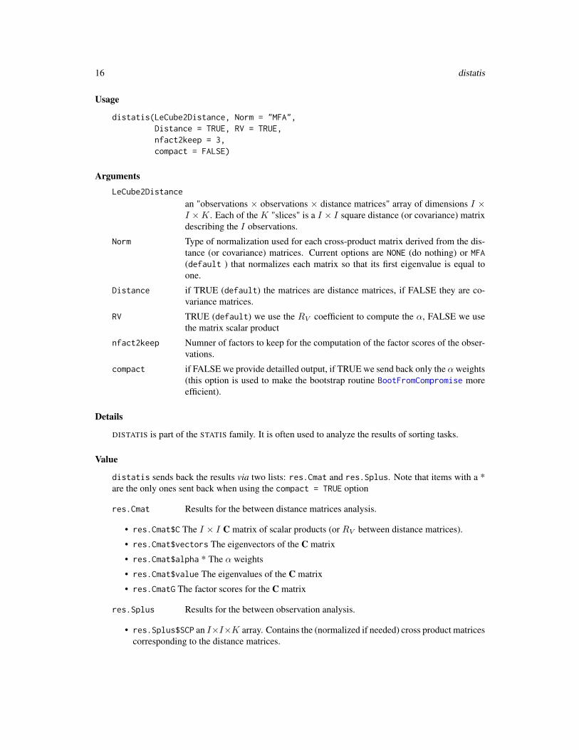
distatis(LeCube2Distance, Norm = "MFA",Distance = TRUE, RV = TRUE,nfact2keep = 3,compact = FALSE)

Arguments

LeCube2Distance

an "observations × observations × distance matrices" array of dimensions I ×I ×K. Each of the K "slices" is a I × I square distance (or covariance) matrixdescribing the I observations.

Norm Type of normalization used for each cross-product matrix derived from the dis-tance (or covariance) matrices. Current options are NONE (do nothing) or MFA(default ) that normalizes each matrix so that its first eigenvalue is equal toone.

Distance if TRUE (default) the matrices are distance matrices, if FALSE they are co-variance matrices.

RV TRUE (default) we use the RV coefficient to compute the α, FALSE we usethe matrix scalar product

nfact2keep Numner of factors to keep for the computation of the factor scores of the obser-vations.

compact if FALSE we provide detailled output, if TRUE we send back only the αweights(this option is used to make the bootstrap routine BootFromCompromise moreefficient).

Details

DISTATIS is part of the STATIS family. It is often used to analyze the results of sorting tasks.

Value

distatis sends back the results via two lists: res.Cmat and res.Splus. Note that items with a *are the only ones sent back when using the compact = TRUE option

res.Cmat Results for the between distance matrices analysis.

• res.Cmat$C The I × I C matrix of scalar products (or RV between distance matrices).

• res.Cmat$vectors The eigenvectors of the C matrix

• res.Cmat$alpha * The α weights

• res.Cmat$value The eigenvalues of the C matrix

• res.CmatG The factor scores for the C matrix

res.Splus Results for the between observation analysis.

• res.Splus$SCP an I×I×K array. Contains the (normalized if needed) cross product matricescorresponding to the distance matrices.

distatis 17

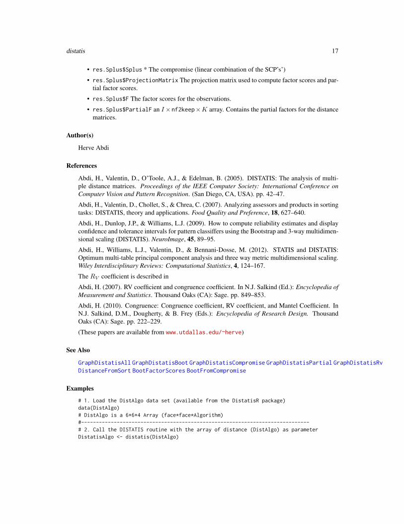
• res.Splus$Splus * The compromise (linear combination of the SCP’s’)

• res.Splus$ProjectionMatrix The projection matrix used to compute factor scores and par-tial factor scores.

• res.Splus$F The factor scores for the observations.

• res.Splus$PartialF an I×nf2keep×K array. Contains the partial factors for the distancematrices.

Author(s)

Herve Abdi

References

Abdi, H., Valentin, D., O’Toole, A.J., & Edelman, B. (2005). DISTATIS: The analysis of multi-ple distance matrices. Proceedings of the IEEE Computer Society: International Conference onComputer Vision and Pattern Recognition. (San Diego, CA, USA). pp. 42–47.




The RV coefficient is described in

Abdi, H. (2007). RV coefficient and congruence coefficient. In N.J. Salkind (Ed.): Encyclopedia ofMeasurement and Statistics. Thousand Oaks (CA): Sage. pp. 849–853.

Abdi, H. (2010). Congruence: Congruence coefficient, RV coefficient, and Mantel Coefficient. InN.J. Salkind, D.M., Dougherty, & B. Frey (Eds.): Encyclopedia of Research Design. ThousandOaks (CA): Sage. pp. 222–229.

(These papers are available from www.utdallas.edu/~herve)

See Also

GraphDistatisAll GraphDistatisBoot GraphDistatisCompromise GraphDistatisPartial GraphDistatisRvDistanceFromSort BootFactorScores BootFromCompromise

Examples

# 1. Load the DistAlgo data set (available from the DistatisR package)data(DistAlgo)# DistAlgo is a 6*6*4 Array (face*face*Algorithm)#-----------------------------------------------------------------------------# 2. Call the DISTATIS routine with the array of distance (DistAlgo) as parameterDistatisAlgo <- distatis(DistAlgo)


18 GraphDistatisAll

GraphDistatisAll This function combines the functionality ofGraphDistatisCompromise, GraphDistatisPartial,GraphDistatisBoot, and GraphDistatisRv.

Description

This function produces 4 plots: (1) a compromise plot, (2) a partial factor scores plot, (3) a bootstrapconfidence intervals plot, and (4) a Rv map.

Usage

GraphDistatisAll(FS, PartialFS, FBoot, RvFS, axis1 = 1, axis2 = 2, constraints = NULL,item.colors = NULL, participant.colors = NULL, ZeTitleBase = NULL, nude = FALSE,Ctr = NULL, RvCtr=NULL, color.by.observations = TRUE, lines = TRUE,lwd = 3.5, ellipses = TRUE, fill = TRUE, fill.alpha = 0.27, percentage = 0.95)

Arguments

FS The factor scores of the observations ($res4Splus$Ffrom distatis)

PartialFS The partial factor scores of the observations ($res4Splus$PartialF from distatis)

FBoot is the bootstrapped factor scores array (FBoot obtained from BootFactorScoresor BootFromCompromise)

RvFS The factor scores of the distance matrices ($res4Cmat$G from distatis)

axis1 The dimension for the horizontal axis of the plots.

axis2 The dimension for the vertical axis of the plots.

constraints constraints for the axes

item.colors A I matrix (with I = # observations) of color names for the observations. IfNULL (default), prettyGraphs chooses.

participant.colors

A I matrix (with I = # participants) of color names for the observations. IfNULL (default), prettyGraphs chooses.

ZeTitleBase General title for the plots.

nude When nude is TRUE the labels for the observations are not plotted (useful whenediting the graphs for publication).

Ctr Contributions of each observation. If NULL (default), these are computed fromFS

RvCtr Contributions of each participant. If NULL (default), these are computed fromRvFS

color.by.observations

if TRUE (default), the partial factor scores are colored by item.colors. WhenFALSE, participant.colors are used.

GraphDistatisAll 19

lines If TRUE (default) then lines are drawn between the partial factor score of anobservation and the compromise factor score of the observation.

lwd Thickness of the line plotting the ellipse or hull.

ellipses a boolean. When TRUE will plot ellipses (from car package). When FALSE willplot peeled hulls (from prettyGraphs package).

fill when TRUE, fill in the ellipse with color. Related to ellipses only.

fill.alpha transparency index when filling in the ellipses. Related to ellipses only.

percentage A value to determine the percent coverage of the bootstrap partial factor scoresto provide ellipse or hull confidence intervals.

Value

constraints A set of plot constraints that are returned.

item.colors A set of colors for the observations are returned.participant.colors

A set of colors for the participants are returned.

Author(s)

Derek Beaton and Herve Abdi

See Also

GraphDistatisAll GraphDistatisCompromise GraphDistatisPartial GraphDistatisBoot GraphDistatisRvdistatis

Examples

# 1. Load the Sort data set from the SortingBeer example (available from the DistatisR package)data(SortingBeer)# Provide an 8 beers by 10 assessors results of a sorting task#-----------------------------------------------------------------------------# 2. Create the set of distance matrices (one distance matrix per assessor)# (ues the function DistanceFromSort)DistanceCube <- DistanceFromSort(Sort)

#-----------------------------------------------------------------------------# 3. Call the DISTATIS routine with the cube of distance as parametertestDistatis <- distatis(DistanceCube)# The factor scores for the beers are in# testDistatis$res4Splus$F# the partial factor score for the beers for the assessors are in# testDistatis$res4Splus$PartialF## 4. Get the bootstraped factor scores (with default 1000 iterations)BootF <- BootFactorScores(testDistatis$res4Splus$PartialF)#-----------------------------------------------------------------------------# 5. Create the Graphics with GraphDistatisAll#

20 GraphDistatisBoot

GraphDistatisAll(testDistatis$res4Splus$F,testDistatis$res4Splus$PartialF,BootF,testDistatis$res4Cmat$G)

GraphDistatisBoot Plot maps of the factor scores of the observations and their boot-strapped confidence intervals (as confidence ellipsoids or peeled hulls)for a DISTATIS analysis.

Description

GraphDistatisBoot plots maps of the factor scores of the observations from a distatis analysis.GraphDistatisBoot gives a map of the factors scores of the observations plus the boostrappedconfidence intervals drawn as "Confidence Ellipsoids" at percentage%.

Usage

GraphDistatisBoot(FS, FBoot, axis1 = 1, axis2 = 2, item.colors = NULL,ZeTitle = "Distatis-Bootstrap", constraints = NULL, nude = FALSE, Ctr = NULL,lwd = 3.5, ellipses = TRUE, fill = TRUE, fill.alpha = 0.27, percentage = 0.95)

Arguments

FS The factor scores of the observations ($res4Splus$F from distatis)

FBoot is the bootstrapped factor scores array (FBoot obtained from BootFactorScoresor BootFromCompromise)



item.colors When present, should be a column matrix (dimensions of observations and 1).Gives the color-names to be used to color the plots. Can be obtained as theoutput of this or the other graph routine. If NULL, prettyGraphs chooses.

ZeTitle General title for the plots.


nude When TRUE do not plot the names of the observations


lwd Thickness of the line plotting the ellipse or hull.

ellipses a boolean. When TRUE will plot ellipses (from car package). When FALSE willplot peeled hulls (from prettyGraphs package).

fill when TRUE, fill in the ellipse with color. Related to ellipses only.

fill.alpha transparency index when filling in the ellipses. Related to ellipses only.

percentage A value to determine the percent coverage of the bootstrap partial factor scoresto provide ellipse or hull confidence intervals.

GraphDistatisBoot 21

Details

The ellipses are plotted using the function dataEllipse() from the package car. The peeled hullsare plotted using the function peeledHulls() from the package prettyGraphs.

Note that, in the current version, the graphs are plotted as R-plots and are not passed back by thefunction. So the graphs need to be saved "by hand" from the R graphic windows. We plan toimprove this in a future version.

Value


item.colors A set of colors for the observations are returned.

Author(s)


References

The plots are similar to the graphs described in:





See Also


Examples

# 1. Load the Sort data set from the SortingBeer example (available from the DistatisR package)data(SortingBeer)# Provide an 8 beers by 10 assessors results of a sorting task#-----------------------------------------------------------------------------# 2. Create the set of distance matrices (one distance matrix per assessor)# (ues the function DistanceFromSort)DistanceCube <- DistanceFromSort(Sort)

#-----------------------------------------------------------------------------# 3. Call the DISTATIS routine with the cube of distance as parameter


22 GraphDistatisCompromise

testDistatis <- distatis(DistanceCube)# The factor scores for the beers are in# testDistatis$res4Splus$F# the partial factor score for the beers for the assessors are in# testDistatis$res4Splus$PartialF## 4. Get the bootstraped factor scores (with default 1000 iterations)BootF <- BootFactorScores(testDistatis$res4Splus$PartialF)#-----------------------------------------------------------------------------# 5. Create the Graphics with GraphDistatisBoot#GraphDistatisBoot(testDistatis$res4Splus$F,BootF)

GraphDistatisCompromise

Plot maps of the factor scores of the observations for a DISTATIS anal-ysis

Description

Plot maps of the factor scores of the observations for a DISTATIS analysis. GraphDistatis gives amap of the factor scores for the observations. The labels of the observations are plotted by defaultsbut can be omitted (see the nude=TRUE option).

Usage

GraphDistatisCompromise(FS, axis1 = 1, axis2 = 2, constraints = NULL, item.colors = NULL,ZeTitle = "Distatis-Compromise", nude = FALSE, Ctr = NULL)

Arguments

FS The factor scores of the observations ($res4Splus$Ffrom distatis).








GraphDistatisCompromise 23

Details

Note that, in the current version, the graphs are plotted as R-plots and are not passed back by theroutine. So the graphs need to be saved "by hand" from the R graphic windows. We plan to improvethis in a future version.

Value


item.colors A set of colors for the observations are returned.

Author(s)


References

The plots are similar to the graphs from


see www.utdallas.edu/~herve

See Also


Examples

# 1. Load the DistAlgo data set (available from the DistatisR package)data(DistAlgo)# DistAlgo is a 6*6*4 Array (face*face*Algorithm)#-----------------------------------------------------------------------------# 2. Call the DISTATIS routine with the array of distance (DistAlgo) as parameterDistatisAlgo <- distatis(DistAlgo)# 3. Plot the compromise map with the labels for the first 2 dimensions# DistatisAlgo$res4Splus$F are the factors scores for the 6 observations (i.e., faces)# DistatisAlgo$res4Splus$PartialF are the partial factors scores##(i.e., one set of factor scores per algorithm)GraphDistatisCompromise(DistatisAlgo$res4Splus$F)


24 GraphDistatisPartial

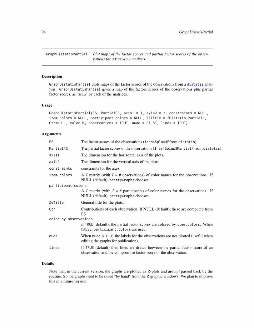
GraphDistatisPartial Plot maps of the factor scores and partial factor scores of the obser-vations for a DISTATIS analysis.

Description

GraphDistatisPartial plots maps of the factor scores of the observations from a distatis anal-ysis. GraphDistatisPartial gives a map of the factors scores of the observations plus partialfactor scores, as "seen" by each of the matrices.

Usage

GraphDistatisPartial(FS, PartialFS, axis1 = 1, axis2 = 2, constraints = NULL,item.colors = NULL, participant.colors = NULL, ZeTitle = "Distatis-Partial",Ctr=NULL, color.by.observations = TRUE, nude = FALSE, lines = TRUE)

Arguments

FS The factor scores of the observations ($res4Splus$Ffrom distatis).

PartialFS The partial factor scores of the observations ($res4Splus$PartialF from distatis)





participant.colors




color.by.observations

if TRUE (default), the partial factor scores are colored by item.colors. WhenFALSE, participant.colors are used.


lines If TRUE (default) then lines are drawn between the partial factor score of anobservation and the compromise factor score of the observation.

Details


GraphDistatisRv 25

Value


item.colors A set of colors for the observations are returned.participant.colors


Author(s)


References

The plots are similar to the graphs from


see www.utdallas.edu/~herve

See Also


Examples

# 1. Load the DistAlgo data set (available from the DistatisR package)data(DistAlgo)# DistAlgo is a 6*6*4 Array (face*face*Algorithm)#-----------------------------------------------------------------------------# 2. Call the DISTATIS routine with the array of distance (DistAlgo) as parameterDistatisAlgo <- distatis(DistAlgo)# 3. Plot the compromise map with the labels for the first 2 dimensions# DistatisAlgo$res4Splus$F are the factors scores for the 6 observations (i.e., faces)# DistatisAlgo$res4Splus$PartialF are the partial factors scores##(i.e., one set of factor scores per algorithm)GraphDistatisPartial(DistatisAlgo$res4Splus$F,DistatisAlgo$res4Splus$PartialF)

GraphDistatisRv Plot maps of the factor scores (from the Rv matrix) of the distancematrices for a DISTATIS analysis

Description

Plot maps of the factor scores of the observations for a DISTATIS analysis. The factor scores areobtained from the eigen-decomposition of the between distance matrices cosine matrix (often amatrix of Rv coefficients). Note that the factor scores for the first dimension are always positive.There are used to derive the α weights for DISTATIS.


26 GraphDistatisRv

Usage

GraphDistatisRv(RvFS, axis1 = 1, axis2 = 2, ZeTitle = "Distatis-Rv Map",participant.colors = NULL, nude = FALSE, RvCtr = NULL)

Arguments

RvFS The factor scores of the distance matrices ($res4Cmat$G from distatis).



ZeTitle General title for the plots.participant.colors



RvCtr Contributions of each participant. If NULL (default), these are computed fromRvFS

Details


Value

constraints A set of plot constraints that are returned.participant.colors


Author(s)


References

The plots are similar to the graphs described in:




mmds 27


The RV coefficient is described in

Abdi, H. (2007). RV coefficient and congruence coefficient. In N.J. Salkind (Ed.): Encyclopedia ofMeasurement and Statistics. Thousand Oaks (CA): Sage. pp. 849–853.

Abdi, H. (2010). Congruence: Congruence coefficient, RV coefficient, and Mantel Coefficient. InN.J. Salkind, D.M., Dougherty, & B. Frey (Eds.): Encyclopedia of Research Design. ThousandOaks (CA): Sage. pp. 222–229.


See Also


Examples

# 1. Load the DistAlgo data set (available from the DistatisR package)data(DistAlgo)# DistAlgo is a 6*6*4 Array (faces*faces*Algorithms)#-----------------------------------------------------------------------------# 2. Call the DISTATIS routine with the array of distance (DistAlgo) as parameterDistatisAlgo <- distatis(DistAlgo)# 3. Plot the compromise map with the labels for the first 2 dimensions# DistatisAlgo$res4Cmat$G are the factors scores# for the 4 distance matrices (i.e., algorithms)GraphDistatisRv(DistatisAlgo$res4Cmat$G,ZeTitle='Rv Mat')# Et voila!

mmds mmds Metric (classical) Multidimensional Scaling (a.k.a PrincipalCoordinate Analysis) of a (Euclidean) Distance Matric

Description

Perform an MMDS of a (Euclidean) distance matrix measured between a set of weighted objects.

MMDS Give factor scores that make it possible to draw a map of the objects such that the distancesbetween objects on the map best approximate the original distances between objects.

Method: Transform the distance matrix into a (double centered) covariance matrix which is thenanalyze via its eigen-decomposition. The factor score of each dimension are scaled such that theirvariance (i.e., the sum ot their weighted squared factor scores) is equal to the eigen-value of thecorresponding dimension. Note that if the masses vector is absent, equal masses (i.e. 1 divided bynumber of objects) are used.


28 mmds

Usage

mmds(DistanceMatrix,masses=NULL)

Arguments

DistanceMatrix . A squared (assumed to be Euclidean) distance matrix

masses A vector of masses (i.e., non negative numbers with a sum of 1) of same dimen-sionality as number of rows of DistanceMatrix.

Value

Sends back a list

LeF factor scores for the objects.

eigenvalues the eigenvalues for the factor scores (ie.a variance).

tau the percentage of explained variance of each dimension.

Contributions give the proporion of explained variance by an object for a dimension.

Author(s)

Herve Abdi

References

The procedure and references are detailled in: Abdi, H. (2007). Metric multidimensional scaling.In N.J. Salkind (Ed.): Encyclopedia of Measurement and Statistics. Thousand Oaks (CA): Sage.pp. 598–605.

(Paper available from www.utdallas.edu/~herve).

See Also

GraphDistatisCompromise distatis

Examples

# An example of MDS from Abdi (2007)# Discriminability of Brain States# Table 1.# 1. Get the distance matrixD <- matrix(c(0.00, 3.47, 1.79, 3.00, 2.67, 2.58, 2.22, 3.08,3.47, 0.00, 3.39, 2.18, 2.86, 2.69, 2.89, 2.62,1.79, 3.39, 0.00, 2.18, 2.34, 2.09, 2.31, 2.88,3.00, 2.18, 2.18, 0.00, 1.73, 1.55, 1.23, 2.07,2.67, 2.86, 2.34, 1.73, 0.00, 1.44, 1.29, 2.38,2.58, 2.69, 2.09, 1.55, 1.44, 0.00, 1.19, 2.15,2.22, 2.89, 2.31, 1.23, 1.29, 1.19, 0.00, 2.07,3.08, 2.62, 2.88, 2.07, 2.38, 2.15, 2.07, 0.00),


print.Cmat 29

ncol = 8, byrow=TRUE)rownames(D) <- c('Face','House','Cat','Chair','Shoe','Scissors','Bottle','Scramble')colnames(D) <- rownames(D)# 2. Call mmdsBrainRes <- mmds(D)# Note that compared to Abdi (2007)# the factor scores of mmds are equal to F / sqrt(nrow(D))# the eigenvalues of mmds are equal to \Lambda *{1/nrow(D)}# (ie., the normalization differs but the results are proportional)# 3. Now a pretty plot with the prettyPlot function from prettyGraphsprettyPlot(BrainRes$FactorScore,

display_names = TRUE,display_points = TRUE,contributionCircles = TRUE,contributions = BrainRes$Contributions)

# 4. et Voila!

print.Cmat Print C matrix results

Description

Print C matrix results.

Usage

## S3 method for class 'Cmat'print(x,...)

Arguments

x a list that contains items to make into the Cmat class.

... inherited/passed arguments for S3 print method(s).

Author(s)

Derek Beaton

30 print.Splus

print.DistatisR Print DistatisR results

Description

Print DistatisR results.

Usage

## S3 method for class 'DistatisR'print(x,...)

Arguments

x a list that contains items to make into the DistatisR class.


Author(s)

Derek Beaton

print.Splus Print S+ matrix results

Description

Print S+ matrix results.

Usage

## S3 method for class 'Splus'print(x,...)

Arguments

x a list that contains items to make into the Splus class.


Author(s)

Derek Beaton

SortingBeer 31

SortingBeer Ten Assessors sorted eight beers for distatis analysis

Description

Provide the data.frame Sort: Data set to be used to illustrated the use of the package DistatisR.Ten assessors sorted eight beers. These data come from the Abdi et al.’ (2007) paper in FoodQuality and Preference. Each column represents the results of the sorting task for one assessor.Beers with the same number were sorted together.

Usage

data(SortingBeer)

Format

a data frame file containing 10 columns, 8 rows plus the names of the rows and the columns.

Source

Abdi et al. (2007). www.utdallas.edu/~herve

References


SortingSpice 21 French assessors sorted 16 blends of Spice for distatis analysis

Description

Provide the data.frame SortSpice: Data set to illustrate the use of the package DistatisR. Tenassessors sorted eight beers. These data come from the Abdi et al.’ (2007) paper in Food Qualityand Preference. Each column represents the results of the sorting task for one assessor. Beers withthe same number were sorted together.

Usage

data(SortingSpice)

Format

a data frame file containing 21 columns, 16 rows plus the names of the rows and the columns.


32 SortingSpice

Source

Chollet et al. (2013). www.utdallas.edu/~herve

References

Chollet, S., Valentin, D., & Abdi, H. (in press, 2013). The free sorting task. In. P.V. Tomasco & G.Ares (Eds), Novel Techniques in Sensory Characterization and Consumer Profiling. Boca Raton:Taylor and Francis.


Index

∗Topic DistatisRChi2Dist, 9Chi2DistanceFromSort, 11DistAlgo, 13DistanceFromSort, 13GraphDistatisBoot, 20GraphDistatisCompromise, 22GraphDistatisPartial, 24GraphDistatisRv, 25mmds, 27SortingBeer, 31SortingSpice, 31

∗Topic bootstrapBootFactorScores, 5BootFromCompromise, 7

∗Topic datasetsDistAlgo, 13SortingBeer, 31SortingSpice, 31

∗Topic distatisdistatis, 15GraphDistatisAll, 18

∗Topic mdsdistatis, 15GraphDistatisAll, 18GraphDistatisCompromise, 22GraphDistatisPartial, 24

∗Topic packageDistatisR-package, 2

∗Topic printprint.Cmat, 29print.DistatisR, 30print.Splus, 30

∗Topic sampleBootFactorScores, 5BootFromCompromise, 7

BootFactorScores, 3, 5, 8, 17, 18, 20BootFromCompromise, 3, 6, 7, 16–18, 20

Chi2Dist, 9Chi2DistanceFromSort, 10, 11CovSTATIS (distatis), 15covstatis (distatis), 15

DistAlgo, 13DistanceFromSort, 3, 13, 17DiSTATIS (distatis), 15distatis, 3, 10–14, 15, 19–21, 23–25, 27, 28DiSTATISR (DistatisR-package), 2DistatisR (DistatisR-package), 2DistatisR-package, 2

GraphDistatisAll, 3, 17, 18, 19, 21, 23, 25,27

GraphDistatisBoot, 3, 6, 8, 17–19, 20, 21,23, 25, 27

GraphDistatisCompromise, 3, 17–19, 21, 22,23, 25, 27, 28

GraphDistatisPartial, 3, 17–19, 21, 23, 24,25, 27

GraphDistatisRv, 3, 17–19, 21, 23, 25, 25, 27

mmds, 3, 9, 10, 27

prettyGraphs, 3print.Cmat, 29print.DistatisR, 30print.Splus, 30

Sort (SortingBeer), 31SortingBeer, 31SortingSpice, 31SortSpice (SortingSpice), 31

33

package ‘distatisr’ - the comprehensive r archive network · package ‘distatisr ... valentin,...

Documents