pacific northwest gridwise™ testbed demonstration · pdf filedemonstration projects part...
TRANSCRIPT

PNNL-17167
Pacific Northwest GridWise™ Testbed Demonstration Projects
Part I. Olympic Peninsula Project
D. J. Hammerstrom, Principal Investigator R. Ambrosio J. Brous T. A. Carlon D. P. Chassin J. G. DeSteese R. T. Guttromson G. R. Horst O. M. Järvegren R. Kajfasz S. Katipamula L. Kiesling N. T. Le P. Michie T. V. Oliver R. G. Pratt S.E. Thompson M. Yao
October 2007
Prepared for the U.S. Department of Energy under Contract DE-AC05-76RL01830 Pacific Northwest National Laboratory Richland, Washington 99352

DISCLAIMER
This report was prepared as an account of work sponsored by an agency of the United States Government. Neither the United States Government nor any agency thereof, nor Battelle Memorial Institute, nor any of their employees, makes any warranty, express or implied, or assumes any legal liability or responsibility for the accuracy, completeness, or usefulness of any information, apparatus, product, or process disclosed, or represents that its use would not infringe privately owned rights. Reference herein to any specific commercial product, process, or service by trade name, trademark, manufacturer, or otherwise does not necessarily constitute or imply its endorsement, recommendation, or favoring by the United States Government or any agency thereof, or Battelle Memorial Institute. The views and opinions of authors expressed herein do not necessarily state or reflect those of the United States Government or any agency thereof.
PACIFIC NORTHWEST NATIONAL LABORATORY
operated by
BATTELLE
for the
UNITED STATES DEPARTMENT OF ENERGY
under Contract DE-AC05-76RL01830
Printed in the United States of America
Available to DOE and DOE contractors from the
Office of Scientific and Technical Information, P.O. Box 62, Oak Ridge, TN 37831-0062;
ph: (865) 576-8401 fax: (865) 576-5728
email: [email protected]
Available to the public from the National Technical Information Service, U.S. Department of Commerce, 5285 Port Royal Rd., Springfield, VA 22161
ph: (800) 553-6847 fax: (703) 605-6900
email: [email protected] online ordering: http://www.ntis.gov/ordering.htm

PNNL-17167
Pacific Northwest GridWise™ Testbed Demonstration Projects
Part I. Olympic Peninsula Project
D. J. Hammerstrom, Principal Investigator R. Ambrosio J. Brous T. A. Carlon D. P. Chassin J. G. DeSteese R. T. Guttromson G. R. Horst O. M. Järvegren R. Kajfasz S. Katipamula L. Kiesling N. T. Le P. Michie T. V. Oliver R. G. Pratt S.E. Thompson M. Yao
October 2007
Prepared for the U.S. Department of Energy under Contract DE-AC05-76RL01830 Pacific Northwest National Laboratory Richland, Washington 99352

PNNL-17167

iii
Abstract
This report describes the implementation and results of a field demonstration wherein residential electric water heaters and thermostats, commercial building space conditioning, municipal water pump loads, and several distributed generators were coordinated to manage constrained feeder electrical distribution through the two-way communication of load status and electric price signals. The field demonstration took place in Washington and Oregon and was paid for by the U.S. Department of Energy and several northwest utilities. Price is found to be an effective control signal for managing transmission or distribution congestion. Real-time signals at 5-minute intervals are shown to shift controlled load in time. The behaviors of customers and their responses under fixed, time-of-use, and real-time price contracts are compared. Peak loads are effectively reduced on the experimental feeder. A novel application of portfolio theory is applied to the selection of an optimal mix of customer contract types.


v
Executive Summary
Pacific Northwest National Laboratory (PNNL) led a field demonstration of smart grid technologies for the U.S. Department of Energy (DOE) and the Pacific Northwest GridWise™ Testbed. The latter is a group composed of several northwest regional utilities, the Bonneville Power Administration (BPA), and PNNL. The overall field demonstration was known as the Pacific Northwest GridWise Testbed Demonstration, composed of two principal projects. This report describes one of these, the Olympic Peninsula Project. The second project, called the Grid Friendly™ Appliance Project, is discussed separately in a companion report.
Purpose and Objectives The purpose of the Olympic Peninsula Project was to create and observe a futuristic energy-pricing
experiment that illustrates several values of grid transformation that align with the GridWise concept. The central principle of the GridWise concept is that inserting intelligence into electric-grid components at the end-use, distribution, transmission and generation levels will significantly improve both the electrical and economic efficiencies within the electric power system. Specifically, this project, tested whether automated two-way communication between the grid and distributed resources will enable resources to be dispatched based on the energy and demand price signals that they receive. In this manner, conventionally passive loads and idle distributed generators can be transformed into elements of a diverse system of grid resources that provide near real-time active grid control and a broad range of economic benefits. Foremost, the project controlled these resources to successfully manage the power flowing through a constrained feeder-distribution circuit for the duration of the project. In other words, the project tested whether it was possible to decrease the stress on the distribution system at times of peak demand by more actively engaging typically passive resources—end use loads and idle distributed generation.
The immediate objectives of the project were to
show that a common communications framework can enable the economic dispatch of dispersed resources and integrate them to provide multiple benefits
gain an understanding of how these resources perform individually and when interacting in near real time to meet common grid-management objectives
evaluate economic rate and incentive structures that influence customer participation and the distributed resources they offer.
Background The significance of the Olympic Peninsula Project may be appreciated in terms of a brief explanation
of the GridWise concept and a review of current electric utility pricing practices.
GridWise Concept. The term GridWise was coined at PNNL to describe the various smart grid-management technologies based on real-time, electronic communication and intelligent devices that are expected to mature in the next several years. By enabling an overall increase in asset utilization, these technologies should be capable of deferring and, in some cases, entirely preventing the construction of

vi
conventional power-grid infrastructure in step with anticipated future load growth. The term GridWise has also been lent to DOE activities and to two consortia pursuing the interoperability of smart grid technologies—the GridWise Alliance and the GridWise Architecture Council.
The GridWise Testbed group was assembled during 2004 to facilitate a field demonstration of the GridWise technologies being developed at PNNL. In addition to DOE, co-funding collaborators included BPA, PacifiCorp, and Portland General Electric. The Olympic Peninsula was suggested by BPA as an ideal location for the field demonstration. The Peninsula is presently served by a capacity-constrained, radial transmission system. The area is experiencing significant population growth, and it already has been projected that power-transmission capacity in the region may be inadequate to supply demand during extremely cold winter conditions. Addressing this region’s situation was also an objective of BPA’s “Non-wires” Program, which shared a common objective with this project of evaluating practical and economical alternatives to new transmission and distribution construction.
Utility Pricing Practices. While fixed electric energy rates still predominate in the United States, price-responsive electricity markets have made inroads. Time-of-use rates, including critical peak rates, have been offered in California and elsewhere to move electricity consumption to periods when the system is not at its peak. Administering time-of-use rates requires advanced utility interval meters that can distinguish and monitor customers’ electricity consumption during peak and off-peak periods. While programs with advanced notification and long time intervals do not mandate the use of automation, adoption of time-of-use rates has been accelerated somewhat by the availability of interval meters and communicating energy-management systems that can automate customers’ responses. Advanced metering and communicating thermostat initiatives are other recent examples of equipment development programs that could hasten the propagation of time-of-use pricing contracts.
To a lesser degree, real-time contracts also have been offered to customers, but these practices have often applied only to large customer loads using relatively long time intervals. The “real-time” prices are communicated up to a day ahead based on advanced markets. For retail electricity sales, the state of available automation supports responses to price intervals down to about 15 minutes. However, these interactions would best be described as one-way, i.e., they do not feed back demand bids except through the actions of aggregators participating in a slower advanced market.
Organized markets for wholesale electricity exist today. The nature of such markets varies greatly with the degree of deregulated market structure region by region. No organized market exists in the Northwest. A few large entities conduct bilateral agreements, and the resulting wholesale market price is not available until the next day.
The Project Market. Against this background, the Olympic Peninsula Project was undertaken to demonstrate further steps in realizing the value of transforming passive end-use loads and distributed generation into active, market-driven resources for power-grid management as well as the practicality of reducing the market clearing time of this process to intervals as short as 5 minutes.
The project’s market was operated at a 5-minute interval to allow the cycling behavior of loads to contribute to load reduction and load recovery. The duty cycle of most appliances, even on peak, is usually sufficiently diverse to allow a load-control signal, such as price, to take advantage of the fact that they turn on and off anyway. By adjusting when and how long loads turn on or off, a great deal of flexibility can be achieved to the benefit of the entire system. Because much of this appliance duty

vii
cycling behavior occurs with a frequency comparable to a 5-minute time scale, it was judged necessary to make the project market operate on a similar time scale to exploit this characteristic of load behavior.
Project Resources Three electric power providers, Public Utility District (PUD) #1 of Clallam County, the City of Port
Angeles, and Portland General Electric, provided the Olympic Peninsula Project with residential, commercial, and municipal test sites. Several other collaborators, specifically IBM’s Watson Research Laboratory and Invensys Controls provided equipment, software, and valuable in-kind project support. Whirlpool Corporation participated by augmenting the controls on project clothes dryers so they would announce high price conditions on their front panels.
Planning for the field demonstration began in late 2004. Equipment was being placed in the field by late 2005, and data were collected from early 2006 through March 2007.
The managed load resources deployed in this project complemented and leveraged the “non-wires” resources that BPA had assembled to mitigate the Olympic Peninsula transmission constraint. The Olympic Peninsula Project included the following controllable assets that were enabled to respond to the project’s energy price signals:
five 40-HP water pumps, distributed between two municipal water-pumping stations, representing a nameplate total load of about 150 kW—The electrical load these pumps placed on the grid was bid into the market incrementally when water-reservoir levels were above a designated height in a water reservoir.
two distributed diesel generators—These two generators (175- and 600-kW) served the facility’s electrical load when feeder supply was insufficient. The biddable resource capacity in this case was the removal of the building electric load (~170 kW) removed from the grid by transferring it to these units. In addition, a small 30-kW microturbine was set up to respond to the two-way market. Unlike the larger generators, the microturbine ran in parallel with the power grid. The market prices offered for the supply of these generator units were based on the actual fixed and variable expenses incurred.
residential demand response for electric water and space heating provided by 112 homes using gateways that supported two-way communications—This residential demand-response system allowed current market prices to be presented to consumers and allowed users to preprogram their automatic demand-response preferences. The residential participants were evenly divided among three types of utility price contracts (fixed, time-of-use, and real-time) and a control group. While all residential electricity was metered, only the appliances in price-responsive homes (~75 kW) were controlled by the project.
Automation was provided by the project to monitor, and in some cases control, each of these resources. Consistent with GridWise principles, all participants and resource operators were provided means to temporarily disable or override project control of their loads or generators. In the cases of residential thermostats and water heaters, appliance owners were provided a means to assign a degree of price responsiveness to their appliances from among lists of 5 to 15 intuitively named comfort settings. In the cases of commercial and municipal resources, the degree of automated price-responsiveness was negotiated with each resource owner.

viii
While not all resources could be co-located on one feeder for this demonstration, the measurement and control of these resources were conducted as if all resided on a common virtual feeder. Throughout the project, these project resources were monitored online at PNNL using distributed energy resource (DER) dashboards as shown in Figure A. This example would show a grid operator how much of a resource is available and how much has already been dispatched. These dashboards allowed project staff to quickly assess the status of the system and its individual resource components. Visualization tools of this type will be critical for grid operators to achieve the widespread adoption of distributed resources.
Figure A. Example Utility Dashboard Summary of Project-Distributed Resource Activity
The central organizing element of the project was a shadow market to provide the incentive signals that encouraged operation of the project’s distributed generation (DG) and demand-response resources to manage local distribution congestion. The project created debit accounts with balances of actual money that were used to cover the shadow market electricity savings earned by the residential customers. The amount of cash they earned and received depended on whether they were operating their household loads in collaboration with the needs of the grid each month. As these customers responded to price signals sent from the shadow market, the cash balances in their debit accounts were reduced at a rate commensurate with the shadow market’s current energy prices for the given market interval. The participants got to keep any money left in the account at the end of each quarter. The project received guidance from BPA to recommend reasonable values for these incentives with limited project budget in mind. Participating homes’ energy consumption histories were also studied before the experiment to establish baseline expectations.

ix
Built upon the region’s Mid-Columbia (MIDC) wholesale electricity price and responsive to the feeder’s real-time load needs and supply availability, the project’s local marginal price reflected the effects of 1) the resources offered and needed at the wholesale level, 2) the feeder’s economical capacity, and 3) the true marginal price of the feeder’s marginal resources. Over time, the price also reflected the effects of customer behaviors as the customers reconfigured their automated responses based on their perceptions of the market and their changing comfort needs.
Discussion of Key Findings This report includes results of extensive data analyses. Several of the project’s most interesting
findings are previewed here.
Distribution Constraint Managed. One of the project’s primary goals was to manage congestion on a feeder. This goal was accomplished. Seasonally, the project imposed a new constraint on the energy that could be imported into the feeder from an external wholesale electricity source. The project then controlled the imported capacity below this constraint for all but one 5-minute interval during the entire project year. Figure B previews this result. On this curve representing the duration of feeder capacity, the feeder supply (the red line) has been limited successfully to 750 kW. Distributed generators provided additional supply (up to about 350 kW at its peak) when needed (green line).
Figure B. Curve Representing the Duration of Feeder Capacity during the 750-kW Feeder Constraint
Market-Based Control Demonstrated. The project controlled both heating and cooling loads. Observation of the project’s residential thermostatically controlled loads for those homes on real-time price contracts revealed a significant, surprising shift in energy consumption. This shift is shown in
10 -5 10 -4 10 -3 10 -2 10 -1 1000
200
400
600
800
1000
1200
1400
Fraction of Hours
Total Demand BidCleared Total SupplyFeeder Supply
Supp
ly (k
W)

x
Figure C. Space-conditioning loads served by the real-time price contracts effectively used energy in the very early morning hours when electricity is least expensive. This effect occurred during both constrained and unconstrained feeder conditions; however, it was more pronounced when the feeder was constrained. This result is remarkably similar to what one would expect for pre-heating or pre-cooling, but these project thermostats had no explicit prediction capability. It is the diurnal shape of the price signal itself that caused this outcome.
Figure C. Shifting of Thermostatically Controlled Load by Price
Peak Load Reduced. As shown in Figure B, the project’s market also deferred and shifted peak load. Unlike time-of-use control, the project’s real-time control operated exactly when needed and with the precise magnitude needed. The magnitude of load reduction under real-time price control increases with the peak itself and with the degree to which the feeder import is constrained. The project conservatively estimated that a 5 percent reduction in peak load was achieved under a 750-kW constraint; 20 percent peak load reduction was easily obtained under a 500-kW feeder constraint.
Internet-Based Control Tested. The project implemented Internet control of its distributed resources though the efforts of project collaborators Invensys Controls and IBM Watson Research Laboratory. Bid and control interactions were communicated via the Internet. Residential thermostats, for example, modified their effective temperature setbacks through a combination of local and central control communicated over the Internet. The project market itself was cleared centrally every 5 minutes. While average project connectivity to these resources was at times sporadic, the resources almost always performed well in default modes until communications could become re-established.
0 3 6 9 12 15 18 21 0
0.50
1.00
Hour of Day
Ave
rage
Spa
ce C
ondi
tioni
ng D
eman
d (k
W)
Actual (14.2 kWh/day, 0.9 peak kW)Baseline (12.2 kWh/day, 0.8 peak kW)
(500-kW feeder constraint period)
0.25
0.75

xi
Distributed Generation Served as a Valuable Resource. The project was particularly successful obtaining useful supply from distributed diesel generators. The project elected to control the generators at their existing emergency-transfer switches. The generators and their protected facilities therefore ran separated, or islanded, from the grid. These generators bid the capacity of the commercial building loads they served; the price they offered was based on actual fixed and variable expenses they would incur by turning on and running. These resources were called upon and used many times during the project. Figure D shows the total distributed generator energy used by the project accumulated by hour of day. The diesel generators were restricted by their environmental licensing to operate no more than about 100 hours per year. This constraint was easily managed by imposing and managing a price premium applied to every market offer made by these resources. Note that many such emergency backup generators lie unused in the United States.
Dis
patc
hed
Dis
tribu
ted
Gen
erat
ion
(kW
h)
Hour of Day Figure D. Total Distributed Dispatch of Energy Generated by Hour of Day
Conclusions The Olympic Peninsula Project was shown to be a unique field demonstration that revealed persistent,
real-time benefits of GridWise technologies and market constructs. The project demonstrated that local marginal retail price signals, coupled with the project’s communications and the market clearing process, successfully managed the bidding and dispatch of loads and accounted quite naturally for wholesale costs, distribution congestion, and customer needs.
The report makes and defends the following assertions:

xii
The project successfully managed a feeder and an imposed feeder constraint for an entire year using these innovative automated technologies.
Market-based control was shown to be a viable, effective tool for obtaining useful price-based responses from single premises.
Market-based control was shown to be a viable, effective tool for obtaining useful price-based responses for the entire feeder.
Peak load reduction was successfully accomplished.
Internet-based communications performed well for the control of distributed resources.
Residents eagerly accepted and participated in price-responsive contract options.
Automation was particularly helpful for obtaining consistent responses from both supply and demand resources.
The ease of participation, automation and ability to override controls, or “friendliness” with which the project invited and practiced demand response may be a key to attaining the needed magnitude of resources.
Real-time price contracts were especially effective in shifting thermostatically controlled loads to take advantage of off-peak opportunities.
Municipal water pumps were successfully incorporated into the responsive demand mix.
While understandably constrained by environmental concerns, the project’s real and virtual distributed generators effectively prevented the overloading of a constrained feeder distribution line during peak periods.
Modern portfolio theory was applied to the mix of residential contract types and should prove useful for utility analysis.
Price-market participants responded to incentives offered through a shadow market. The project demonstrated that demand response programs could be designed by establishing debit account incentives without changing the actual energy prices offered by energy providers.
The Olympic Peninsula Project demonstrated a suite of GridWise technologies on a common feeder to the point of providing a clear and quantitative demonstration of their effectiveness. The project was planned at a large enough scale to offer unambiguous evidence that resources could be bid into an electricity market to provide, in principle, solutions for a constrained power-delivery infrastructure that did not involve constructing new poles and wires. While technological challenges were found and noted, the project found no fundamental technological limitations that should prevent the application of these technologies again and at larger scale.

xiii
Acronyms
AHU air-handling unit
APEL Advanced Process Engineering Laboratory
BAS building automation system
BPA Bonneville Power Administration
CPB Cyber-Physical Business (systems)
CPP critical peak price
DDC direct digital control
DER distributed energy resource
DG distributed generation
DOE U.S. Department of Energy
DSL digital subscriber line
EIOC Electrical Infrastructure Operations Center
EMS energy management system
GFA Grid Friendly™ appliance
HVAC heating, ventilation and air conditioning
IBM International Business Machines
iCS Internet Scale Control System
JCI Johnson Control
LCD liquid crystal display
LCM load control module
MIDC Mid-Columbia
MSL Marine Sciences Laboratory
OLE object link and embedding
O&M operations and maintenance
OPC OLE for process control
PGE Pacific Gas and Electric
PNNL Pacific Northwest National Laboratory
PUD public utility district
RTP real-time price

xiv
T&D transmission and distribution
TOU time-of-use
VAV variable air volume
VPN Virtual Private Network

xv
Contents
Abstract ........................................................................................................................................................ iii
Executive Summary ...................................................................................................................................... v
Acronyms...................................................................................................................................................xiii
1.0 Introduction to the Olympic Peninsula Project .................................................................................. 1.1
1.1 Background Information ............................................................................................................ 1.1
1.2 Project Objectives ...................................................................................................................... 1.4
1.3 Participants and Collaborators.................................................................................................... 1.5
1.4 Approach .................................................................................................................................... 1.5
2.0 Local Marginal Energy Price Market................................................................................................. 2.1
2.1 Introduction to Transactive Control ........................................................................................... 2.1
2.2 Two-Sided Real-time Market with Clearing .............................................................................. 2.2
2.3 Source and Load Bids ................................................................................................................ 2.4
2.4 Transactive Control for Thermostatically-Controlled Equipment.............................................. 2.5
2.5 Water Heater Controls................................................................................................................ 2.7
3.0 Residential Load Control ................................................................................................................... 3.1
3.1 Project Locations........................................................................................................................ 3.1
3.2 Recruitment Process ................................................................................................................... 3.1
3.3 Participant Qualifications ........................................................................................................... 3.2
3.4 Incentives ................................................................................................................................... 3.3
3.5 Participant Obligations............................................................................................................... 3.4
3.6 Contract Types and the Assignments of Contract Types ........................................................... 3.4
3.7 Residential Control Equipment .................................................................................................. 3.8
3.8 Installation of Project Equipment............................................................................................. 3.14
3.9 Duration of Experiment............................................................................................................ 3.15
4.0 Commercial Building Load Control................................................................................................... 4.1
4.1 Traditional Building-Space Conditioning Controls.................................................................... 4.1
4.2 Transactive Building Control ..................................................................................................... 4.2

xvi
4.3 Case Study of Transactive Control............................................................................................. 4.3
5.0 Municipal Water Pump Load Control................................................................................................ 5.1
5.1 Transactive Market for Real-Time Energy Control ................................................................... 5.1
5.2 Pump Load Control and Communications ................................................................................. 5.1
5.3 Detailed Method of Bidding....................................................................................................... 5.4
5.4 Pump Load Market Behavior ..................................................................................................... 5.6
6.0 Distributed-Generator Control ........................................................................................................... 6.1
6.1 Project Distributed-Generator-Resource Description................................................................. 6.1
6.2 Generator Bid Strategy............................................................................................................... 6.2
6.3 Detailed Method of Bidding....................................................................................................... 6.3
6.4 Observations of Distributed-Generator Market Behavior .......................................................... 6.6
6.5 Conclusions Concerning Distributed-Generator Resources ....................................................... 6.8
7.0 Data Analysis Results ........................................................................................................................ 7.1
7.1 Chosen Equipment Settings ....................................................................................................... 7.1
7.2 Network Performance ................................................................................................................ 7.2
7.3 Residential Incentives and Savings ............................................................................................ 7.3
7.4 Utility Billing ............................................................................................................................. 7.6
7.5 Effect of Wholesale Energy Price .............................................................................................. 7.9
7.6 Residential Load Shapes .......................................................................................................... 7.12
7.7 Commercial Load Shape .......................................................................................................... 7.19
7.8 Feeder Capacity........................................................................................................................ 7.19
7.9 Project Peak-Load Reduction................................................................................................... 7.22
7.10 Consumer Surplus .................................................................................................................... 7.27
7.11 Production Dispatch ................................................................................................................. 7.30
7.12 Contract Type Mixtures for Achieving Desirable Risk / Benefit Ratios.................................. 7.30
8.0 Perspectives........................................................................................................................................ 8.1
8.1 Utility Perspective ...................................................................................................................... 8.1
8.2 System Integrator Perspective .................................................................................................... 8.5
8.3 Equipment Manufacturer Perspective ........................................................................................ 8.9
8.4 Residential Participant Perspective .......................................................................................... 8.11

xvii
9.0 Conclusions........................................................................................................................................ 9.1
10.0 References ........................................................................................................................................ 10.1
11.0 Other Suggested Reading................................................................................................................. 11.1
Appendix A............................................................................................................................................... A.1


xix
Figures
1.1. Project Communication Schematic................................................................................................... 1.8
2.1. Example 3-Day History for the 5-Minute Two-Sided Clearing Market ........................................... 2.3
2.2. Control of Imposed Distribution Constraint Using Transactive Control .......................................... 2.4
2.3. Illustration of Bid and the Response Strategy for Thermostatically Controlled Loads .................... 2.5
3.1. Contract Types Awarded to Participants by Preference Expressed .................................................. 3.7
3.2. Invensys GoodWatts™ System Components ................................................................................... 3.9
3.3. Load Control Module (LCM) and a Participant's Water Heater ..................................................... 3.10
3.4. GoodWatts™ Energy Meter, as Installed by Trained Utility Electricians...................................... 3.11
3.5. Some Project Dryers Were Configured to Display Energy (“En”) Alert Signals........................... 3.12
3.6. Residential Participant Using His GoodWatts™ Web Site ............................................................ 3.12
3.7. Example Screen from the GoodWattsTM Web Site User Interface ................................................. 3.13
4.1. Example Control Loop Schematic .................................................................................................... 4.2
4.2. Effect of Transactive Control on Zone Temperatures and Set Points............................................... 4.5
4.3. Zone Bid, Market Clearing Price, and Mean Price of the Electricity ............................................... 4.6
5.1. Pumps at the Sekiu Water Pumping Station ..................................................................................... 5.2
5.2. Water Reservoir Serviced by the Sekiu Pumping Station................................................................. 5.2
5.3. The Sekiu Pump Station Located Across the Street from Clallam PUD Facilities .......................... 5.3
5.4. Control Panels at the Sekiu Pumping Station ................................................................................... 5.3
5.5. Pump Controller Hardware............................................................................................................... 5.4
5.6. Pump Control Diagram..................................................................................................................... 5.5
5.7. Sekiu Bid Strategy Based on Reservoir Height ................................................................................ 5.6
5.8. Sekiu Pump Control Observations for January 20, 2007.................................................................. 5.7
6.1. PNNL's 600-kW Caterpillar Diesel Generator in Sequim, Washington........................................... 6.1
6.2. PNNL’s 175-kW Kohler Generator and Automatic Transfer Switch............................................... 6.2

xx
6.3. Upper Generator Power Transfer Switch at PNNL’s MSL .............................................................. 6.3
6.4. Generator Control Diagram .............................................................................................................. 6.4
6.5. Distribution of Accepted Generator Bid Prices for the Two MSL Generators................................. 6.7
6.6. Distribution of Accepted Generator Capacity Bids for the Two MSL Generators........................... 6.8
6.7. Average MSL Site Loads by Hour of Day........................................................................................ 6.9
7.1. Distribution of Selected Residential Thermostat Limit Settings ...................................................... 7.1
7.2. Network Telemetry Performance Statistics (15-minute Intervals) ................................................... 7.3
7.3. Monthly Residential Participant Incentive Payment Distribution .................................................... 7.4
7.4. Monthly Savings Estimates by Contract Type.................................................................................. 7.5
7.5. Residential Participant Average Monthly Energy Use ..................................................................... 7.6
7.6. Residential Monthly Utility Revenue by Contract Type .................................................................. 7.7
7.7. Residential Participant Average Monthly Energy Price by Contract Type ...................................... 7.8
7.8. MIDC Wholesale Electricity Price Behavior.................................................................................. 7.10
7.9. Diurnal Residential Load Shapes for each Season and Day Type by Contract Type ..................... 7.13
7.10. Real-time Market Shifting of Thermostatically Controlled Residential Load................................ 7.19
7.11. Served and Managed Distribution Load ......................................................................................... 7.20
7.12. How Real-time Price Can Flatten Load .......................................................................................... 7.21
7.13. Distribution Operations During Critically Constrained Feeder Conditions.................................... 7.22
7.14. Feeder Load Duration Curves......................................................................................................... 7.23
7.15. Peak Reduction and Imposed Feeder Capacities During the Project.............................................. 7.25
7.16. Supply Duration Curves.................................................................................................................. 7.26
7.17. Definition of Consumer Surplus on a Market Closing Diagram .................................................... 7.28
7.18. Consumer Surplus by Month .......................................................................................................... 7.29
7.19. Seasonal Consumer Surplus by Hour of Day ................................................................................. 7.29
7.20. Distributed Generation Dispatch .................................................................................................... 7.31
7.21. Efficient Frontier and Other Portfolio Weightings ......................................................................... 7.32

xxi
7.22. Two Pure Distributions (Blue) and Distributions for Mixes of the Two (Green)........................... 7.33
7.23. Efficient Frontier Mixtures of Two Pure Distributions .................................................................. 7.34
7.24. Peak Energy Use for Season and Time of Day for the Duration of the Project.............................. 7.35
7.25. Gross Margin of Utility per Day per Residential Customer for the Project Year........................... 7.36


xxiii
Tables
2.1. Example of Water Heater Curtailment Probability for Values of kW ................................................ 2.8
3.1. Time-of-use and Critical Peak Rates ................................................................................................ 3.6
3.2. Residential Contract Choices............................................................................................................ 3.8
3.3. Appliance Control Summary by Residential Contract Type .......................................................... 3.14
3.4. Appliance Comfort Settings and Resulting kW and kT Values......................................................... 3.15
5.1. Water Pump Control Prior to Project Involvement........................................................................... 5.5
6.1. Variables Used to Calculate Distributed Generator Offers............................................................... 6.6
7.1. Snapshot Summary of Real-time Contract Participants’ Thermostat Comfort Settings................... 7.2
7.2. Snapshot Summary of Real-time Contract Participants’ Water Heater Comfort Settings................ 7.2
7.3. Mean Daily Energy Consumption per Home.................................................................................... 7.7
7.4. Summary Application of Distribution Capacity ............................................................................. 7.19
7.5. Average Peak Reduction During Constrained Project Periods....................................................... 7.25

xxiv

1.1
1.0 Introduction to the Olympic Peninsula Project
This document describes the planning, commissioning, and results of a project that was part of the Pacific Northwest GridWise™ Testbed Demonstration. The Pacific Northwest GridWise Testbed Demonstration was a major collaborative research activity in the GridWise program being conducted by Pacific Northwest National Laboratory (PNNL) for the U.S. Department of Energy (DOE). The Olympic Peninsula Project is one of the two major Pacific Northwest GridWise Testbed demonstrations designed to show that advanced information-based technologies can increase asset utilization and reliability of the power grid in support of the national GridWise agenda. This section provides background context to explain the rationale for the Olympic Peninsula Project in addition to the project’s objectives, participants, approach, and planning.
1.1 Background Information
The demand for electricity is expected to continue its historical growth trend far into the future. To meet this growth with traditional approaches would require adding power generation, transmission, and distribution that may cost in aggregate up to $2,000/kW on the utility side of the meter. The amount of capacity in generation, transmission, and distribution generally must meet peak demand and must provide a reserve margin to protect against outages and other contingencies. The nominal capacity of many power-grid assets is typically used for only a few hundred hours per year. Traditional approaches for maintaining the adequacy of the nation’s power generation and delivery system are characterized by sizing system components to meet peek demand, which occurs only a few hours during the year. Thus, overall asset utilization remains low, particularly for assets located near the end-user, i.e., in the distribution portion of the system.
1.1.1 The Role of Information Technologies
The increased availability of energy-information technologies can play an important role in addressing the asset utilization issue cost-effectively. Patrick Mazza (2005) provided an excellent summary of this and many other potential benefits that the smart grid holds for the Northwest. PNNL’s efforts in this area were accelerated upon the publication of a Rand Science and Technology report (Baer et al. 2004) which estimated that $57 billion savings could be realized by applying smart technologies throughout the nation’s electric generation, transmission, and distribution systems over the next 20 years.
Historically, power-supply infrastructure has been constructed to serve load, a purely passive element of the system. Today, information technology has been developed to the point of allowing larger portions of the demand-side infrastructure to function as an integrated system element. Thus, for the first time, distributed electric load can be made to actively participate in grid control and protection functions as well as real-time economic interactions. The collective application of these information-based technologies to the U.S. power grid is the backbone of the GridWise concept (DOE 2007; PNNL 2007; GridWise Alliance 2007). GridWise technologies are expected to allow more power to be delivered through existing delivery infrastructure and reduce the rate and cost of future system expansion to accommodate load growth. At the same time, these technologies will increase grid reliability by using the

1.2
load resources on the customer’s side of the meter to make the grid inherently more efficient (Butler 2007), stable, and reconfigurable.
1.1.2 GridWise Implementation
The transformational nature and broad scope of the GridWise concept will require substantial field testing and demonstration before widespread adoption can occur. Such a profound transformation requires field testing before wide-scale adoption to establish the worth of a variety of technologies and reveal possible shortcomings in their implementation and integration. This transformation enables the integration of a diverse suite of distributed resources. These are anticipated to function in conjunction with existing utility assets to produce an aggregate value much greater than the sum of benefits provided by individual components or subsystems. Key aspects expected of the GridWise implementation are that it will
provide benefits at multiple levels of the system from the same distributed resources (i.e., generation and wholesale markets, transmission, and distribution)
integrate multiple types of distributed resources (e.g., distributed generation and demand response)
use “real-time” communication of market-like incentives to obtain cooperative, voluntary responses from customers.
It is unlikely that the concept will gain widespread acceptance by demonstrating individual technologies separately and in isolation. Thus, demonstrating GridWise benefits requires testing at the integrated system level.
It is equally important to demonstrate how new business models and regulatory solutions can overcome institutional barriers to a GridWise implementation. Stakeholders, such as electricity consumers, utility service providers, public utility commissions, and other interested parties need to be involved in testing these propositions, as well. This requirement expands the scope of the GridWise transformation well beyond the level of a purely technological demonstration.
The GridWise concept has achieved, to date, a remarkable coalescence of interest on the part of utilities, regulators, and power and information technology developers. The Olympic Peninsula Project represents a significant and tangible demonstration of multiple technologies acting in concert to show that aspects of the GridWise concept are both practical and achievable.
1.1.3 Project Focus
The Olympic Peninsula Project is one of two significant demonstrations that were conducted to address Pacific Northwest GridWise Testbed objectives. The project was undertaken to demonstrate how industrial, commercial, and residential demand-response and backup generation resources can be dispatched through real-time communication of cost information and the end-use value of electrical services. These values were based on an experimental shadow market reflecting realistic wholesale costs and incentives to relieve transmission congestion.
The second project, documented in a companion report (Hammerstrom et al. 2007), was a field test of Grid Friendly™ appliance (GFA) technology. That effort was designed to show how well autonomous,

1.3
fast-acting, short-term underfrequency shedding of residential appliance loads can be deployed as a significant resource for improving the frequency stability of the power grid without perceptibly inconveniencing the end user.
These projects were designed to demonstrate many functional aspects of the future power grid envisioned by the GridWise concept for the next decade. These two projects have considerable mutually complementary value in terms of the demand response each achieved. In addition, some degree of overlap was designed into the projects by arranging for them to share some of the resources on the Olympic Peninsula. This report focuses exclusively on the Olympic Peninsula Project.
1.1.4 Olympic Peninsula Project Rationale
Both the geographical topography and the particular electric-grid configuration on the Olympic Peninsula in Washington State contribute its being an ideal location for demonstrating GridWise technologies in the Pacific Northwest. The Olympic Peninsula is dominated by the centrally located Olympic mountain range. This topography has forced human settlement predominantly at lower altitudes within an area ranging a few miles inland from a lengthy coastline bounded by the Strait of Juan de Fuca and the Pacific Ocean. The largest of several small cities and towns situated in this area is Port Angeles with a population now in excess of 20,000 (18,397 in the 2000 Census). The region is not heavily industrialized. However, the area’s population is increasing quite rapidly, resulting in a projected load growth of more than 20 MW per year.
Port Angeles is supplied by two 230-kV circuits forming the Shelton-Fairmount connection supplied by the Olympia Substation on the Bonneville Power Administration (BPA) grid. Power transmission to communities west of Port Angeles is achieved at lower voltages over a long and essentially radial system. The principal threat to power delivery on the Olympic Peninsula is an outage of a major transmission line to Olympia. If this were to occur under extra-heavy winter load conditions, the Olympic Peninsula could experience voltage instability and even collapse.
BPA has studied options for reinforcing the Olympic Peninsula transmission system for many years. Various system and institutional constraints have presented challenges to designing economical reinforcement using conventional construction that will both support load growth and maintain adequate supply reliability. Because of the unique circumstances of its configuration, load density and diversity, and service conditions, both the transmission and distribution (T&D) portions of the Olympic Peninsula power delivery system have become, from BPA’s perspective, prime candidates for “non-wires” enhancement solutions. This approach calls for offsetting future needs for new T&D construction with more cost-effective alternative measures, including demand-side management and improved use of existing infrastructure. BPA has published energy-efficiency and transmission-technology roadmaps (BPA 2006) to focus its future research in these technology areas.
A number of resources have been already developed and deployed by BPA to reduce demand on the Olympic Peninsula transmission constraint, including a commercial and industrial Demand ExchangeSM, a distributed generation project involving backup generators, and a co-located residential demand-response project. As a result of ongoing load growth, these resources may be needed in the event of severe cold weather as soon as 2008. In this context, all additional resources in whatever amount added by the Olympic Peninsula Project offer real, tangible benefits to the region’s grid.

1.4
In principle, GridWise benefits can be demonstrated anywhere on the grid. However, the value of field demonstrations in areas where the grid is currently robust or less constrained might be appreciated only at an academic level of interest. Siting a test bed where a real need for alternative supply solutions is already apparent amplifies the prospect that any demonstrated benefits may be clearly recognized and rapidly adopted. These considerations provided a strong incentive for selecting the Olympic Peninsula grid as a prime project site where GridWise technologies address a present need and can be unambiguously demonstrated. Through this demonstration, the Pacific Northwest has the potential of becoming a leader in deploying such technologies for the benefit of its own power system and pointing the way for GridWise implementation on a national scale.
1.2 Project Objectives
The fundamental objectives of the Olympic Peninsula Project are to
show that a common communications framework can enable economic dispatch of dispersed resources and integrate them to provide multiple benefits
gain an understanding of how these resources perform individually and when interacting in near real time to meet common grid-management objectives
evaluate economic rate and incentive structures and other socio-political issues that influence customer participation and the distributed resources they offer.
Constrained by finite resources, no practical demonstration can reasonably be expected to achieve all potential goals in these three areas. However, the most important desired outcomes of this effort include
demonstrating how transmission and distribution capital investment can be deferred
demonstrating the important role that demand response will play in the future and illustrating its potential benefits in the residential and commercial sectors
demonstrating how distributed generators can contribute benefits to the system beyond the energy they produce
illustrating how distributed resources can enhance the stability and reliability of the system.
Some additional objectives of the Olympic Peninsula Project were that it would
demonstrate alternative solutions to power-delivery problems with broad national applicability
help achieve valuable GridWise research goals
be able to display the achievement of system benefits in quasi-real time using a compelling visual interface
serve as an expandable platform to integrate diverse, geographically dispersed regional demonstration efforts.
A central tenet of the GridWise concept is that there is no single technological “silver bullet” that will verify the best, most cost-effective use of power grid assets. Rather, one must integrate a broad range of new, distributed resource technologies with existing grid assets. Achieving an appreciable level of

1.5
technological integration is considered to be among the most challenging objectives of the Olympic Peninsula Project.
1.3 Participants and Collaborators
The Olympic Peninsula Project was managed by PNNL with the participation and collaboration of utilities, commercial technology providers, and experts on regional transmission organizations and experimental economics. Three electric power providers, BPA, Public Utility District (PUD) #1 of Clallam County, and the City of Port Angeles, provided the Olympic Peninsula Project with residential, commercial, and municipal test sites. Several other collaborators, specifically IBM’s Watson Research Laboratory and Invensys Controls, provided valuable products and in-kind project support.
Other project participants included Preston Michie (Consultant, Preston Michie & Associates, LLC) and Dr. Lynne Kiesling, who provided guidance for designing the market structure and setting up the market experiment, respectively.
1.4 Approach
A range of dispersed supply-side and demand-side resources were deployed at various locations on the Olympic Peninsula transmission route. These resources were integrated into a virtual physical operating and market environment, backed with real cash consequences that allowed a degree and quality of experimentation previously unavailable to the GridWise program. By linking and co-managing demand and distributed generators in the same economic-dispatch system, their relative cost efficiencies, their degree of response, and the synergies between them were measured as functions of time-of-day, day-of-week, time-of-year, and duration of curtailment. Major sections of this report contain detailed discussions of how the distributed resources introduced here were recruited and incorporated into the Olympic Peninsula Project.
1.4.1 Distributed Resources
The assets introduced in this project were deployed to complement and leverage BPA’s investment in “non-wires” solutions that address the growing Olympic Peninsula transmission constraint. The following are brief statements of how each of the distributed resources was deployed.
Distributed Generation and Demand Response at Marine Sciences Laboratory (MSL). PNNL operates the MSL campus in Sequim, Washington, which has two diesel backup generators, a 175-kW unit and a newer 600-kW unit, that had been part of a BPA non-wires distributed generation project conducted for BPA by contractor Celerity (BPA 2004). These two generators were integrated into the market dispatch system of the Olympic Peninsula Project using the existing Johnson Controls building energy-management system at the MSL and its automatic transfer switch. The project calculated and provided local marginal costs to these resources to modify their control based on price signals from the shadow market. The distributed generators bid their actual costs for starting and running for short intervals, including their automated management of environmentally permitted run times.
Transactive Commercial Building Demand Response. The office building of the MSL also responded to project market price signals using PNNL’s transactive building control technology, in which

1.6
thermostatically controlled zones within the building were made to compete amongst themselves for limited energy resources. Each zone bid for the resource according to the variance between its temperature set point and its actual zone temperature. The zones having winning bids were granted air flow through control of their variable air volume (VAV) flow dampers.
Automated Residential Demand Response. The Olympic Peninsula Project recruited 112 homes to install energy-management systems that supported two-way communications. This allowed the project’s current market prices to be distributed to residents and provided a user-programmable automatic demand-response capability for residential water heaters and thermostatically-controlled heating, ventilation and air conditioning (HVAC) systems. End-use data collection was also incorporated so that both automated and manual demand response of various appliance loads could be measured for some residential clothes dryers, water heaters, and HVAC systems. The thermostat control provided setback demand-response conservation benefits during both the cooling and heating seasons.
The practical realization of these residential demand-response resources approached 1.5 kW per home, or about 160 kW in total. Participants were encouraged to tailor and pre-program their desired automated demand responses via Web sites accessible from their homes’ personal computers. Thereby, participants could select their own preferred balance between energy cost savings and comfort. The project provided participants educational materials concerning the programming of such automated responses and the voluntary efforts they could pursue during the project to achieve even greater benefits. Warning lights and visible indicators alarmed during periods of high electricity prices at thermostats and at some clothes dryers.
In addition, 50 clothes dryers and 25 water heaters in these homes were equipped with GFA underfrequency load-shedding capability (Hammerstrom et al. 2007).
Advanced Process Engineering Laboratory (APEL) Microturbine Distributed Generation. The project also incorporated a 30-kW microturbine resource that had already been made remotely controllable through prior contract work for BPA. This generator represented the project’s only paralleled generator, meaning it and the facility it served remained grid-connected while the generator unit ran. Because the startup costs incurred by the microturbine were small, the microturbine was the most active distributed generation resource used in the project.
Hoko River and Sekiu Municipal Water Pump Demand Response. PUD #1 of Clallam County water department worked closely with the project to provide and observe control of water-reservoir levels at its Hoko River and Sekiu water pumping stations. Control was implemented via Johnson Control systems at these two sites to control a total of five 40-hp municipal water pumps. The control traded off small variations in allowed water-reservoir levels for the control of times during which pumps were allowed to run. This control was made responsive to the shadow-market price-control signals of the project.
Virtual Distributed Generation Resources. Due to cost and time constraints, the project also incorporated virtual distributed generator resources of various sizes into the shadow market in addition to the real generators. The operation of the virtual distributed generators was simulated emulating the same control objectives and constraints applied to the project’s real generators. Environmental restrictions applied to the virtual generators as for the real ones.
Further discussion of the project’s generator and load resources will be presented in this report using four logical chapter divisions:

1.7
• Chapter 3.0: Residential Load Control
• Chapter 4.0: Commercial Building Load Control
• Chapter 5.0: Municipal Water Pump Load Control
• Chapter 6.0: Distributed Generator Control.
1.4.2 Shadow Market
The central organizing element of the project was to implement a near-real time shadow market to provide the incentive signals that induced operation of the project’s distributed generators and demand-response resources. The project integrated real resources into a virtual market that allowed the resources to compete and respond to pricing signals. This part of the project employed the skills of Dr. Lynne Kiesling, formerly of the International Foundation for Research in Experimental Economics associated with Northwestern University, to help design an incentive system based on her expertise and experiences in experimental economics.
To avoid potentially lengthy delays and regulatory hurdles that would be encountered designing special rates for customers and implementing them in actual utility billing systems, the project’s shadow market created, in effect, a debit account that customers could earn by operating household appliances in collaboration with the needs of the grid. Residential electric customers were given real cash balances at the beginning of each month. As these customers responded to price signals sent from the virtual market, their cash balances were reduced or remained unchanged, depending on the value of their demand responses. Quarterly, the project disbursed the remaining funds in these accounts to the participants. This virtual market environment, backed with real cash consequences for customers, allowed meaningful experimentation with various market constructs and price signals.
One should not miss the point that this project represents the first limited-scale practice of a two-way clearing market with 5-minute clearing intervals at the retail level.
The Olympic Peninsula Project received guidance from Preston Michie to assist the project team, including BPA and the utilities involved, in defining reasonable values for these incentives. For this experimental market to produce results with any validity, the price signals must realistically reflect the structure and magnitude of price signals and rates designed to induce demand response in the future. This approach also allowed the incentive structures to be varied across customers or time to experiment with their effect on customer response.
The shadow market system was set up to communicate the real-time (5-minute) aggregate local marginal price for electricity to each customer involved. These marginal prices included the costs for wholesale power in the Western Interconnection, as indicated by the behaviors of the Mid-Columbia (MIDC) price, and market incentives to relieve the transmission constraint as were determined by the automated resolution of load bids and supply offers in the market.
IBM contributed their Internet Scale Control System (iCS), a Web-Sphere™ based middleware software, as the foundation of the shadow market system. The market features of the real-time contract operations were carried out centrally, but these functions were seamlessly integrated by International Business Machines (IBM’s) middleware into the project as if the features had been provided locally at every home gateway. The software enabled the display of both incentive signals and resource responses in

1.8
near-real time on the project Web site and allowed the project to browse historical results. The middleware software also allowed dynamic re-configuration of the system by adding or removing residential home components as well as user preferences and settings. Figure 1.1 shows the principal elements of the communication system.
Chapter 2 will present a more complete discussion of the energy markets used in this project and how these markets worked.
Figure 1.1. Project Communication Schematic
1.4.3 Demonstrating Distribution Benefits with a Virtual Feeder
The Olympic Peninsula Project was designed to indicate how peak loads on distribution feeders can be managed to avoid the need for local capacity expansion. To do this, the widely distributed real assets of the test bed were integrated into a virtual distribution environment where they appear and perform as resources available on a single capacity-constrained feeder. The shadow market was employed to signal these assets to operate and to manage this constraint as if they were actually all co-located on such a virtual feeder.
This feeder’s capacity constraint could be arbitrarily modified during the experiment to throttle the activity of the control imposed by the project’s market. Three different capacity constraints were asserted during the project’s duration.

2.1
2.0 Local Marginal Energy Price Market
The Pacific Northwest GridWise Testbed Demonstration designed and implemented an experimental local marginal price market on the Olympic Peninsula and gathered residential, commercial, and municipal loads and distributed generators to bid into and respond to the local marginal pricing market there. This chapter summarizes the design and operation of this market and how the distributed resources were controlled by this market during the period from early 2006 through March 2007.
2.1 Introduction to Transactive Control
By transactive control (referred to as contract nets by Smith [1980]), the project refers broadly to market-based building control systems, whether those systems are used locally within a single building or facility or throughout a region. The project chose a two-way market in which both suppliers and loads submit bids. This approach is remarkably scalable. It can successfully be applied within a building, as was done in this project to create a market competition between space conditioning zones in the project’s MSL (refer to Chapter 4 for more details), and it can be applied regionally as the project did at multiple residential and commercial building locations on the Olympic Peninsula.
Consumers who participated in the real-time market submitted demand price bids for the expected power to be used by them during the next 5-minute interval. These bids were placed at the price at which they would be willing to curtail the stated power consumption. Most consumers submitted at least two bids for each 5-minute interval, one for their controllable, curtailable load and the other for their uncontrolled, non-curtailable load. Consumers’ uncontrollable, uncurtailable load power was always bid at $9999—infinity from the perspective of the project’s market.
The one generator that was able to run in parallel with the power grid always submitted bids for the maximum nameplate generation capacity it could supply. The price of its supply offer consisted of all costs that would be incurred to start the unit and included the effects of minimum allowable runtime and environmental permits. Minimum runtimes were enforced by bidding a high start-up price, followed by very low running prices for the first few 5-minute periods until the minimum runtime expired. The running price was then escalated until it met the steady run cost, usually within one-half hour. The complete formulas by which generators automatically bid will be presented in Section 6.3.
Backup generators that could not generate back into the distribution network were required to bid as consumers. Thus, non-paralleled backup generators always bid on the demand side, not the supply side, of the market. However, they could only bid the capacity of the load that they were backing up at the time of the market clearing. The offer, however, was also calculated to reflect the effects of actual startup costs, runtime costs, minimum runtimes, and environmental constraints.
The retail market was cleared every 5 minutes. All demand bids and supply offers were sorted by price while summing their cumulative capacity, thus producing the demand and supply curves for that market. The intersection of the load and supply curves always occurred in one point, which was published back to all bidders as the market’s clearing price and cleared power quantity. If the curves did not intersect, such as when the uncurtailable load quantity exceeded the sum of all supply bid quantity, then the market cleared at $9999 (infinity). This occurred only once in more than 100,000 market

2.2
clearings during this project, corresponding to a single 5-minute interval during which the unresponsive demand did indeed exceed all available supply.
2.2 Two-Sided Real-time Market with Clearing
The best way to convey the system operation of the project’s real-time energy market is by examining an example. Figure 2.1 shows an example of a two-sided market clearing diagram 3-day “snapshot” for the historic operation of the Pacific Northwest GridWise Testbed Demonstration between October 30 and November 1, 2006. The loads’ price bids are arranged from highest to lowest as one proceeds rightward toward higher total cumulative load. The supply price bids are shown ascending in price with increasing cumulative supply.
Supply. The extended, flat base price, leftmost on the supply curve, represents the base price for energy that can be delivered by the constrained feeder. The simulated feeder constraint is shown arbitrarily assigned by the project at 500 kW in this figure (the location of the first step in the supply curve). This much power is readily imported into the region at a cost assigned equal to the bulk wholesale cost of electricity plus a small premium. The project chose to assign this wholesale cost by projecting hourly MIDC wholesale price data from the prior day, according to data collected from Dow Jones. The projection of day-ahead price was problematic only on Mondays and Sundays, for which day-ahead markets were unavailable before 2007. On these two week days, wholesale prices were projected without dynamics from known recent average and peak daily wholesale prices.
The higher priced plateaus toward the right of the supply curve are the offers received from the project’s real and virtual distributed generators. Due to cost and schedule constraints, with the exception of a single 30-kW microturbine, these distributed generators on the supply curve were simulated to emulate the market behaviors and performance of real distributed generators of various sizes.
Demand. The “infinite” demand-side bids by the uncontrolled project loads (vertical line leftmost on the demand curve) represent all loads of those residents who were not assigned to the real-time price contracts and also the dishwashers, refrigerators, lighting, and other loads in real-time contract homes that were not configured to bid into the market. The next large steps usually corresponded to the offers of the real and virtual emergency-backup diesel generators that bid the capacities of the loads they served. The multiple small steps even farther to the right corresponded to the responsive pumping loads and responsive residential loads in real-time contract homes.
Clearing Process. The project’s published local marginal price for each interval is the price at which the load and supply curves intersected. The historic 5-minute local marginal prices are displayed as green diamonds in Figure 2.1. It can be seen that the recent history in this figure includes higher prices when the transmission constraint would have been exceeded and higher-priced distributed generation resources were started to avoid exceeding the constraint. As shown at present, however, those small loads bidding to the right of the intersection choose not to operate, and total system load is being held at the feeder constraint capacity (500 kW).

2.3
Cumulative Served Capacity (kW)
Pric
e ($
/MW
h)
1000
900
800
700
600
500
400
300
200
100
0 0 100 200 300 400 500 600 700 800 900 1000
Uncontrollable Demand
MIDC Price Index Level
Parallelable Distribution Generator Offers
Responsive LoadsCleared Price, Capacity
(for Oct. 30 – Nov. 1, 2006)
Backup Generator Offers
Figure 2.1. Example 3-Day History for the 5-Minute Two-Sided Clearing Market
In general, if the total consumers’ demand was less than the feeder’s capacity, the retail price was the same as the wholesale price. When the feeder’s capacity was exceeded, the retail price would rise according to how the retail market cleared. Those loads to the right of the intersection defer their operation also to help manage the constraint. However, all bidding loads share the responsibility and any discomforts equitably over time because the automated bid process dynamically prioritizes the loads according to their present needs. The loads are queued from highest bid to lowest. The highest bidding loads are permitted to run; low-bidding loads are compete unsuccessfully in the market and do not operate. By using transactive control throughout the project’s region, a single local marginal price was sufficient to manage both load and generation resources in the region.
It is also interesting to view this 3-day period in another way. Figure 2.2(a) shows the time history of loads and local marginal prices for the same 3-day period used in Figure 2.1. The total cleared load (black line) is the sum of the unresponsive loads on the system (i.e., things like household refrigeration and small appliances that were not controlled by the project, the blue line) and the controlled loads. When the total load approaches the feeder capacity limit (horizontal red line), the local marginal price (the black line of Figure 2.2(b)) increases sharply and helps keep the dynamic system load below the limit.
On the supply side of the market, the higher clearing local marginal prices become enticing to generators, which eventually turn on to increase the total allowable capacity of the region. The startup of distributed generators is concurrent with the instances where the total cleared load significantly exceeds the transmission constraint.

2.4
Figure 2.2. Control of Imposed Distribution Constraint Using Transactive Control
2.3 Source and Load Bids
Having discussed an example of the system-wide, aggregate behaviors of the resources as they participated in the project’s real-time market, the discussion now addresses the general methods by which the project’s resources calculated their bids and offers into this market. The general approaches can be organized as
• bids and responses from thermostatically controlled loads
• responses from non-thermostatically controlled, non-bidding loads
• distributed generator resource offers.
The first two of these methods will be discussed in the next sections of this chapter concerning thermostatically controlled loads and residential water heater loads. The discussion of the methods by which distributed generators formulated their bids will be deferred until Section 6.3.
Load
(kW
) Pr
ice
($/M
Wh)
Hour in Past 0 -20 -40 - 60 - 80 - 10 -30 -50 - 70
(a)
(b)
1000
500
0
1000
500
0
Uncontrolled Load
Controlled Load Feeder Constraint
Retail
(Oct. 30 – Nov. 1, 2006)
Wholesale

2.5
2.4 Transactive Control for Thermostatically-Controlled Equipment
The discussion in this section can be applied to the controls of space heating and cooling at both the residential and commercial buildings that participated in the project. The approach extends also to the control of the municipal water-pump loads controlled by the project if the temperature is replaced by reservoir height as the principal control input for determining the loads’ bids.
Thermostatically controlled heating and cooling modifies conventional controls by explicitly using market information (bids and clearing prices). A bid curve functionally relates cost of service and an occupant’s comfort. The bid curve in the example illustration (Figure 2.3) is derived from the 24-hour mean and standard deviation market price and minimum and maximum temperature limits. The standard deviation and average of the clearing price will be continually evaluated and updated.
Before the math is discussed, it must be made clear that the occupant was required to make only two simple decisions. The occupant had to select a preferred temperature setting Tset for each scheduled occupancy period. For each occupancy period, the occupant also selected a comfort setting from among a set of alternatives. Invisible to the occupant, each comfort setting assigned pairings of elasticity factors and temperature limits (i.e., kT_L, Tmin and kR_H, Tmax). The exact pairings of comfort settings and these parameters will be greatly clarified later by Table 3.4.
Pric
e
TemperaturesetT min max
Cur
rent
Zon
e Te
mpe
ratu
re
Bid Price
Market Price
Des
ired
Tem
pera
ture
Max
imum
Tem
pera
ture
Lim
it
Min
. Tem
p. L
imit
Bid Curve
currentset,a T T
Average Price
TT
Adj
uste
d Se
t Poi
nt
Paverage + kT_H σ
Paverage - kT_L σ
Pbid
Paverage
Pclear
(Cooling Mode Example)
Figure 2.3. Illustration of Bid and the Response Strategy for Thermostatically Controlled Loads
Assume that the high-temperature limit Tmax corresponds to kT_H standard deviations from the mean price. Remember that the value kT_H is automatically determined with the user’s selected comfort setting. The values of kT_L and kT_H need not be identical for the upper and lower parts of the bid curve. If both kT_H and kT_L are infinitely large, the thermostat would function like a normal thermostat unaffected

2.6
(inelastic) by grid conditions and the behaviors of the market. In this cooling (air conditioning) example, a high value of kT_H will lead to relatively high bids when the zone temperature exceeds the desired zone temperature Tset, which a high bid will help make sure that the zone cooling bid will win the right to become satisfied. If kT_L and kT_H are small (elastic behavior), bids from the thermostatically controlled load deviate little from the mean price, and current temperatures are permitted to vary throughout a relatively large temperature range (from Tmin to Tmax) as the market’s cleared price changes.
Although the illustration assumes that the price of electricity is changing in real time, transactive thermostat control has been also successfully adapted to work for time-of-use, day-ahead, and critical peak pricing structures with minor modifications.
The following paragraphs and equations define step-by-step procedures by which the thermostatically controlled loads bid and respond for the next market interval:
The first step is to measure the current indoor zone temperature Tcurrent and calculate the consequent bid price Pbid. The bid price is based on the slope of the bid curve and difference between the current zone temperature Tcurrent and the desired zone temperature set point Tset. The corresponding bid price depends on additional parameters that are defined by the chosen comfort setting (kT_L, kT_H, Tmax and Tmin), while the mean market clearing price and standard deviation of the market clearing price are external inputs calculated from the recent historical performance of the market.
( )setit
Tsetcurrentaveragebid TT
kTTPP−×
−+=lim
σ (2.1)
where Pbid is the bid price, Paverage is the mean price of electricity for the last 24-hour period, σ is the standard deviation of the electricity price for the same period, and kT and Tlimit are chosen from kT_L, kT_H and Tmin, Tmax, depending on where Tcurrent presently resides on the bid curve. The reader will gain a better understanding of the relationship between comfort settings and these parameters in Section 3.7.
For the market, the project defined the mean and standard deviation price parameters over the prior 24-hour window. The intention of doing so was to track the energy price trends closely without necessarily tracking the diurnal behaviors of that price. By using averaged price parameters, the algorithm becomes adaptive. Relative high and low price definitions are based on recent historical information. Independent of any absolute price thresholds, the algorithm may be similarly applied where prices are high, where prices are low, and where the prices are tending to increase. The use of a recent standard deviation automatically adapts a load’s bid to be effectively scaled to be competitive in the present market.
The next step is to post the resulting bid to the market. The market then establishes the market clearing price using this and the many other bids and offers, as has been described in the previous section. Incidentally, the market may be cleared either externally, as was done for this project, or internally at the building or system level. When clearing internally, the systems within a building compete for an internal, rather than an external, reallocation of costs and services.
After receiving the resulting posted market clearing price, the adjusted zone set point Tset,a is calculated. One should observe again the graphical interpretation of this step on Figure 2.3.

2.7
σ×−
−+=T
setitaverageclearsetaset k
TTPPTT lim
, )( (2.2)
The final step is to reset the thermostat’s zone set point to the new adjusted zone set point. Once the set point is adjusted, the thermostat’s conventional control takes over. In the illustration of Figure 2.3, the adjusted cooling set point falls below the current temperature Tcurrent, meaning that there presently exists an opportunity to cool the given space at an acceptable energy cost. This process continues for each market clearing cycle. The notion of a single zone temperature set point no longer exists because the set point can be affected by the market as well as participants’ selected comfort settings. Note that Tset,a can be higher or lower than the desired set point Tset based on the market clearing price. In cooling mode, lowering the adjusted set point Tset below the desired set point will increase the energy consumption as one takes advantage of low energy costs.
Transactive control can support more aggressive pre-cooling and pre-heating functions. (For example, lowering the set point below what would normally be comfortable is done to pre-cool.). For some dynamic rate structures (i.e., time-or-use), the future price is known a priori; however, in the case of real-time pricing, the future price is unknown. To pre-heat or pre-cool with real-time pricing, one should have the ability to forecast future prices. Pre-cooling and pre-heating comfort settings were offered to participants during this project, but these comfort settings were problematic and were not well understood by residential participants. Several participants objected when their space heaters elevated their homes’ temperatures above their set points in the middle of winter nights when prices were minimal. These participants were then advised to select higher comfort settings without pre-heating and pre-cooling features.
Although there are multiple required steps to successfully implement the project’s transactive control process for thermostatically controlled loads, all the steps and responses were fully automated with energy-management systems deployed in conjunction with the IBM-distributed control system. Ideally, most of these steps should be performed in the thermostat itself.
The steps in this section and the illustration of Figure 2.3 can be made to apply well to the control of the project’s municipal water-pump loads by simply replacing the temperature input variable by reservoir height.
2.5 Water Heater Controls
This section summarizes the water heater control strategy used in the Olympic Peninsula Project. Water heaters differ from the thermostatically controlled loads described in Section 2.4 in that they have no temperature measurement with which they could formulate their present need for electricity as bids into a market. The project therefore formulated a means by which water heaters could opportunistically respond to market prices without having to formulate and submit any bids. The resulting approach describes a probability function by which the water heater will be granted a probabilistic opportunity to run, depending on the relative magnitude of a cleared market price. Water heaters were the only loads to respond in this way during the Olympic Peninsula Project; however, other loads (e.g., pool pumps and battery chargers) could perhaps have been configured to respond similarly.

2.8
The basic water heater control requires that the circuit be interrupted with increasing likelihood as the clearing price exceeds the reported historic average electricity price. The greater the difference between the clearing price and average, the more likely the water heater circuit will be interrupted. The water heater owner selects a comfort setting and its consequent weighting factor (i.e., a kW factor), which either attenuates or amplifies the effect of the probability function.
The probability of turning off the water heater is determined by the formula
( )( )[ ]
otherwiser
rPPNkdxekr clearW
PxP
Wclear
;0
0;5.0,,21
21 2
2
2
=
≥−=⎥⎥⎦
⎤
⎢⎢⎣
⎡−= ∫−∞
−−
σσπ
σ (2.3)
where N is the cumulative normal distribution, and the factor kW is defined through the participant’s selection of a comfort setting (see Table 3.4). The parameter r may be used to test the probability of turning the water heater off by comparing it to a uniformly generated random number between 0 and 1. If r is greater than this random number, the water heater is to be curtailed.
See Table 2.1 for examples of the probability of water heater curtailment given various values of comfort setting kW and several cleared market prices. Specific values of cleared market price Pclear are provided for the case where the mean cleared market price over the past day has been $75/MWh, and its standard deviation is $25/MWh. The likelihood of the water heater load becoming shed increases with the cleared energy price Pclear and with the factor kW. As shown, the water heaters never curtailed when the price was below average; it is always advantageous for the water heaters to heat their water when the price is below average.
Table 2.1. Example of Water Heater Curtailment Probability for Values of kW (Pmean = 75, σ = 25)
Factor kW
Multiples of σ Pclear ($/MWh) 0 0.5 1.0 1.5 2.0 -3 0 0.0% 0.0% 0.0% 0.0% 0.0% -2 25 0.0% 0.0% 0.0% 0.0% 0.0% -1 50 0.0% 0.0% 0.0% 0.0% 0.0% 0 75 0.0% 0.0% 0.0% 0.0% 0.0% 1 100 0.0% 17.1% 34.1% 51.2% 68.3% 2 125 0.0% 23.9% 47.7% 71.6% 95.4% 3 150 0.0% 24.9% 49.9% 74.8% 99.7%

3.1
3.0 Residential Load Control
The purpose of this section is to explain the Olympic Peninsula Project’s interactions with its residential participants and the residential loads controlled by the project.
3.1 Project Locations
With assistance from BPA, the project identified opportunities and obtained permissions to recruit residential participants in and near Sequim and Port Angeles, Washington, on the Olympic Peninsula. These regions were located in the two utility service territories operated by PUD #1 of Clallam County and the City of Port Angeles. Late in the recruitment effort, several homes were also recruited in the service territory of Portland General Electric in Gresham, Oregon. Eventually, 112 residential participants were successfully recruited to participate in the Olympic Peninsula Project.
3.2 Recruitment Process
Potential participants for the project were recruited with the assistance of their local utility companies. The utilities targeted their recruitment efforts toward potential participants who would likely have high-speed Internet service, primarily electric HVAC space heating and cooling, an electric water heater, and an electric dryer.
The project received mailing lists for these potential participants from the utility companies. Recruitment letters were mailed to potential residential participants on the Olympic Peninsula. The recruitment letters listed the participation requirements and asked them to visit a project Web site to provide the project their contact information and answer a series of questions that were later reviewed to determine if the participant met the participation requirements. The project intentionally over recruited at this point, knowing that some of the invited applicants would become disqualified by later screening efforts to be conducted by the project’s automated Web site and by follow-up phone interviews. Despite much effort expended to recruit 200 participants, the project only located and successfully signed up 112 qualified participants.
Soon after the recruitment letters were mailed, the project’s Web site began receiving visits. The questions asked applicants at the Web site are detailed in a flow chart, which was useful during the design of the Web site—see Appendix Figure A.1. The purpose of these questions was to automate the pre-qualification process for residential applicants. The qualification criteria will be further discussed in the following sections.
Early project interactions with participants indicated a need for still more follow-up screening questions, and phone interviews were therefore conducted by the project with each screened applicant. Confusion had been created among ours and the similar “PowerShift” program that was being conducted simultaneously by BPA in the same geographical area. The project’s initial inclination and efforts were to disqualify those who had already qualified for the BPA program; however, despite best efforts, several homeowners qualified for and participated in both programs.

3.2
Some residents lacked very basic knowledge about their appliances and Internet services. For example, some did not know for certain whether they used electric or gas water heat. Others could not accurately describe the nature of their existing Internet service and whether the service was broadband or dialup. With practice, the project learned to efficiently discern applicants’ eligibility. Applicants were asked, for example, whether they received a bill from a gas company to quickly discern whether they might have gas rather than electric water heater service. Often, the name of the Internet service provider alone could discern the nature of a home’s Internet service.
The project also encountered challenges understanding the nature of space-heating equipment in applicant’s homes. The preference was for applicants having HVAC systems for both the heating and cooling of their homes. Unfortunately, the cool Olympic Peninsula has relatively little air conditioning load, and few suitable homes were found to have HVAC systems. However, the interaction of the project’s home automation equipment was obtained through thermostats, so the project ultimately also accepted applicants with all or part of their homes’ heating loads served by resistive heating as long as the home was served by one, or at most two, thermostats. The project attempted to clarify the types of home heating systems in the applicants’ homes by inquiring how many thermostats controlled the homes.
The project had initially predicted that participants would eagerly pursue the offered incentives and would be quickly and easily recruited, but initial recruitment efforts did not receive the desired level of response. The following additional methods were used to recruit more applicants to participate:
• town-hall meeting—In January 2006, the project led two town hall meetings in an effort to recruit more participants, answer questions, and assist applicants with completing their project paperwork.
• radio show interview—In November 2005, two PNNL project staff and a Clallam County PUD staff were interviewed by KNOP radio talk show from Port Angeles, Washington. This exposure generated several more sign-ups on the project’s Web site.
• newspaper advertisements—The project placed advertisements in the Peninsula Daily News with broad readership on the Olympic Peninsula.
• solicitation by mail—The project conducted several mailings targeted to utility regions or desirable broadband Internet service customers.
• word of mouth—The value of informal networks cannot be overlooked. One Olympic Peninsula participant single-handedly recruited at least four other participants.
3.3 Participant Qualifications
In this section, the residential-applicant qualities the project sought are summarized. As was stated earlier, it often took multiple interactions with applicants to determine whether they met these criteria:
• The applicant must be served by one of the two participating utilities. Two utilities had agreed to informally cooperate with the project. Utilities accepted the responsibility to replace participant revenue meters with the project’s advanced meters.
• The applicants had to own and occupy their own homes throughout the project duration. The project required participants’ permissions to modify the homes’ electrical service and to attach

3.3
control boxes with fasteners to walls. Unoccupied homes were avoided because the project wished to test the interactions of occupants with provided equipment.
• The applicant must have HVAC space conditioning (later relaxed to the applicant having not more than two central thermostats). The project would interact with participating homes through one, or at most two, thermostats. The project wished to affect both heating and cooling loads.
• The applicant must have at least one 30-gallon or larger electric, not gas or solar, water heater. Project load-control modules were to be installed between the electric water heaters and 240-VAC service. Only water heaters with reservoirs have the thermal energy storage that can be used for peak reduction in a way that would be accepted by participants.
• The applicant must receive and subscribe to broadband Internet service. The project’s home gateway communicated with the project via broadband Internet connections. The project desired to interact with applicants who would be savvy enough to use their Internet user interfaces and to take project surveys online.
• Each applicant’s revenue meter had to be within 60 feet of the home. This criterion was adopted soon after installations began, at which time the project learned this limitation of the premise wireless communications. At that distance, the wireless signal became unreliable.
• Optionally, the applicant must use an electric, not gas, dryer. Some applicants were chosen to also participate in the Grid Friendly Appliance Project (Hammerstrom et al. 2007). At a sample of these homes, the project investigated the broadcast of energy price information at the clothes dryers’ user interfaces.
3.4 Incentives
The project offered applicants 1) the use of project equipment for the management and monitoring of their home water heaters and space heating and 2) a total of $150, on average, cash earnings, more or less, depending on the occupants’ responses to the energy signals provided to them by the project. These incentives were offered in the initial recruitment letters to applicants and were carefully stated in the contract between participants and the project. Participants earned more than this amount due to an extension of the project one additional quarter beyond what had been initially planned.
At the beginning of each project month, each participant’s project account was refilled with an amount of cash. The amount of cash was unique for each participant, based on the participant’s assigned contract type and his/her historical consumption of electric energy at his/her home. During the month, cash was removed by the project from each account commensurate with the time and contract price at which each participant consumed electricity. The remainder, if any, was returned each project quarter to the participant by check. Participants’ monthly accounts were never allowed to become negative.
The participants’ incentive accounts were unaffected by customers’ normal electric utility bills. The incentive accounts only dealt with the differential electricity costs and benefits that the customers would have incurred had they truly been under contracts that might have differed from the fixed-price contract offered by their local electric providers.

3.4
Quarterly, the project reviewed these accounts and calculated and mailed the project incentive checks. Some modifications were needed at these times to target the promised average compensation. These modifications were justified by the project because of limited project funds and the significant variability some of these contracts exhibited with seasonal temperature variations.
3.5 Participant Obligations
Each participant became contractually obligated to 1) make reasonable allowances for access by the project into homes to install, fix, or uninstall project equipment, 2) take initial and final surveys provided them by the project, and 3) occupy the home and interact with the provided project equipment. Participants were required to inform the project in advance if they would be unable to complete their project participation for any reason.
3.6 Contract Types and the Assignments of Contract Types
Participants were offered three types of electricity contracts—fixed, time-of-use (TOU) with critical peak price (CPP), and real-time price (RTP). Participants requested and were assigned to these three contract types and a fourth experimental control group in roughly equal numbers. The experimental price contracts did not change the existing obligations the customers had with their existing electric service providers.
The following quoted educational information was provided to the participants concerning these contracts at the time they were asked to state their first and second preferences:
“Fixed price program contract—This choice requires little or no involvement from you and little to no change in your electricity usage patterns. You are most likely to receive a small program payment with this contract choice.
“The price of electricity under the fixed-price program contract will remain constant, regardless of when you use electricity or how much you use at any one time—just like the bill you currently receive from your local utility. In this program contract, there is no incentive for changing your usage when electricity is in short supply. However, you may affect your program bill by using more or less electricity.
“Tips to minimize your program bill under this program contract:
“Perform energy-efficiency strategies to save energy, such as turning down your thermostat, replacing incandescent light bulbs with compact fluorescent light bulbs, installing low-flow showerheads, switching from warm to cold water cycles in the washing machine, installing storm windows, checking and installing sealing and weather stripping, etc.”
The project’s fixed price of $81/MWh (8.1¢/kWh) was selected and used for these contract participants. This price was determined by BPA project collaborators based on a forward market price for a comparably sized load, plus a small service provider markup.
Following is the invitation for applicants to participate in the project’s time-of-use contracts:

3.5
“Time-of-use/critical peak program contract—This program contract choice will require a moderate level of consumer involvement and change in your electricity usage patterns. You are most likely to receive a moderate program payment with this contract choice. By changing the time at which you use electricity, you may be able to reduce your program bills.
“The price of electricity under the time-of-use/critical peak program contract will vary between three program rates:
“Off-peak: this program rate will apply mid-day, night, and weekend hours when demand for electricity is typically at its lowest. The program rate during these times will be lower than what you currently pay your local utility.
“On-peak: this program rate will apply in the weekday early morning and early evening hours when the demand for electricity is typically at its highest. The program rate during these times will be higher than what you currently pay your local utility.
“Critical peak: this program rate will apply during times of power shortages or emergencies on the electrical grid (representing disruptions on the power grid, times of increased congestion on major transmission lines, etc.). The program rate during these times will be much higher than the “on-peak” rate described above. There will be a limit to the number of these critical peak events for the year, each lasting no more than four hours, and you will be notified at least one day in advance so you can respond appropriately.
“Your equipment will receive these price signals, and you can set your equipment to respond automatically to these rates as you desire. You can also take voluntary actions to reduce your household’s energy use during critical peak times. For your convenience and comfort, you can override your equipment settings at any time.
“Tips to minimize your program bill under this program contract:
“Choose the maximum economy selection when setting up your thermostat set points using the Invensys GoodWatts™ user interface.
“Avoid overriding your controller.
“Pay attention to notices of upcoming critical peak price events and be prepared to respond.
“Eliminate all unnecessary use of electricity during critical peak periods.”
Those residential participants assigned to the time-of-use with critical peak pricing contracts were invited to automate their homes’ responses for on-peak, off-peak, and critical peak periods using the energy-management equipment supplied them by the project. Prices were assigned by the project for each of these three periods, and these time-of-use prices and corresponding periods remained constant at least through a season. Participants were able to select from multiple comfort settings, much as has been described for those on real-time price contracts. During the on-peak periods, including that for a critical peak period, the homes’ thermostats would revert to a user-selected temperature setback, which would permit the homes’ temperatures to coast and avoid or defer energy consumption. Water heater operation could be curtailed during on-peak and critical peak scheduled periods. A critical peak event was called only once during the project on November 1, 2006, from 2:00 AM to 6:00 AM. Invensys Control

3.6
GoodWatts system had been designed for time-of-use interactions, and the equipment was quickly and easily configured for participants on this contract.
The time-of-use periods and their retail rates are summarized in Table 3.1.
Table 3.1. Time-of-use and Critical Peak Rates
Season Period Times (Pacific w/DST) Price (¢/kWh) Spring
(1 Apr–24 Jul) off-peak on-peak critical
9:00a–5:59p; 9:00p–5:59a 6:00a–8:59a; 6:00p–8:59p
(not called)
4.119 12.150 35.000
Summer (25 Jul–30 Sep)
off-peak on-peak critical
9:00p–2:59p 3:00p–8:59p
(called 1 Nov 2:00a–6:00a)
5.000 13.500 35.000
Fall/Winter (1 Oct–31 Mar)
off-peak on-peak critical
9:00a–5:59p; 9:00p–5:59a 6:00a–8:59a; 6:00p–8:59p
(not called)
4.119 12.150 35.000
“Real-time pricing program contract—This choice requires the greatest consumer involvement and the greatest change in your electricity usage patterns. You are most likely to receive the largest program payment with this contract choice.
“The price of electricity under the real-time pricing program contract will vary every five minutes and somewhat unpredictably during the course of the day, week, and year. Participants in this program contract can set and adjust an automatic response to the price signals by going to the Internet and choosing between maximum comfort, maximum economy, or some level of response in between. At any time, you can press a button on your thermostat to override your pre-set responses. Some equipment also will signal if prices are unusually high so that you can choose whether to use electricity or not during that program price period. By using less electricity, especially when energy prices are high, you may be able to lower your program bills substantially.
“Tips to minimize your program bill under this program contract:
“Program the Invensys GoodWatts™ thermostats for your heating and cooling system and water heater for maximum economy.
“Avoid overriding your system settings.
“Voluntarily reduce your overall electricity usage as much as possible when the warning light is flashing, indicating that prices are unusually high
“Perform energy-efficiency strategies to save energy, such as those listed above.”
Behaviors of automated controls in the real-time price contract homes were described in Section 2.4 for thermostatically controlled space conditioning and in Section 2.5 for water heater controls.
“Control group—In addition to these three groups, a certain number of participants will be randomly assigned to a control group for the course of the program. If you are selected to be in the control group, equipment will be installed in your home, but you will not have a program account, program contact, or

3.7
program bills. Control-group members will receive $150 over the course of the project in appreciation of their participation, regardless of how they use electricity.”
Figure 3.1 shows participants’ first, second, and assigned contract types. As shown, participants showed the strongest preference for real-time pricing contracts. This preference was somewhat surprising, but the project had perhaps oversold the contract by stating that participants could earn the greatest incentives by participating in this contract type.
The project’s contract assignment methodology first chose the control-group members at random, and then maximized the number of participants that got their first or second choices through an iterative random reassignment procedure. A control group assignment was made, but subjects were not offered the opportunity to volunteer for the control group. According to this method, a score is generated based on the square difference between numbers of customers receiving desirable assignments in each contract type. One randomly chosen subject is then changed from one group to another, and if the score is improved, the change is adopted. This process was repeated up to 1000 times until the score could no longer be improved. The final arrangement was adopted as the final customer contract membership.
At the conclusion of this assignment process, 49 percent of participants were granted their first choices, 16 percent received their second choice, and the remaining 36 percent were granted neither their first nor second choices. This last group is deceptively high because it included control-group assignments that could not have been requested by the participants. Final group memberships were nearly equal in size between the four contract groups. See Table 3.2. The final assignment of a specific program contract was communicated to each participant.
NULL CTRL FIXED TOU RTP0
10
20
30
40
50
60
Contract Type
Num
ber o
f Par
ticip
ants
First ChoiceSecond ChoiceAssigned
Figure 3.1. Contract Types Awarded to Participants by Preference Expressed

3.8
Table 3.2. Residential Contract Choices
Preference Fixed Time-of-Use Real-time None Control first 10% 32% 58% 3% –
second 14% 48% 14% 27% – assigned 26% 26% 28% – 23%
3.7 Residential Control Equipment
The project conducted a competitive request for proposals for energy-management-system equipment that would perform requested monitoring and control functions for residential thermostats and electric water heaters. Invensys Controls won this competition and entered into a contract to provide the project its needed equipment and services. Figure 3.2 shows the components of the Invensys GoodWatts™ system. The system had been designed primarily for time-of-use contract types and had been recently successfully applied by BPA at Ashland, Oregon (BPA 2004).
Each participant was provided by the project
• a home gateway
• a Virtual Private Network (VPN) for those homes possessing digital subscriber line (DSL) broadband connections
• a water heater load-control module
• a communicating thermostat
• an advanced revenue meter.
A sample of participants was also provided a load-control module for their clothes dryers.
The system’s home gateway communicated wirelessly with the other system hardware and via Internet to the project and Invensys back-end servers. The gateway and VPN resided near each home’s personal computer. The gateway’s firmware contained some of the necessary project functions that defined its interactions with the thermostat and water heater. The gateway’s firmware was successfully updated in the field several times during the project to update or correct system performance. The gateway maintained a memory of component actions and duties such that the system components could function acceptably for a while even if Internet connectivity had been severed.
The home gateway required that a VPN box be installed in locations having DSL Internet connectivity. Additional thermostats were used as wireless repeaters in several locations where distances or materials prevented successful wireless communication between system components. The gateways, VPNs, and modems were found to need periodic re-booting by the participants during the project.
3.7.1 Water Heater Load-Control Module
The water heater load-control module contains a 240-VAC switch and a means for wireless communications that permit it to receive, store, and respond to the curtailment commands and schedules that it receives. The load-control module could also tell the project whether the water heater was active or

3.9
idle as a load. A load module was installed between each electric water heater and 240-VAC home service in each project home by licensed electricians. Based on users’ occupancy schedules, time-of-use schedules, critical peak events, or real-time contract commands, the load-control module switch could break the 240-VAC circuit, causing the water heater, if active, to shed or defer its load. A water heater load-control module is shown installed at a project home in Figure 3.3.
(GoodWatts Web Site, Courtesy Invensys Controls)
Figure 3.2. Invensys GoodWatts™ System Components
3.7.2 Communicating Thermostat
Participants’ existing thermostats were replaced by GoodWatts wireless communicating thermostats. The thermostat was able to receive curtailment commands and was able to maintain simple scheduled occupancy modes with or without wireless connectivity to the remainder of the system. The liquid crystal display (LCD) panel of the thermostat displayed the system’s present occupancy setting and status and alerted the participant to special occurrences like high energy price conditions. At the project’s conclusion, participants chose to either have their project thermostats left in place or removed and replaced by another. One interesting observation was the challenge in finding installers who were both qualified electricians and knowledgeable of thermostat-control wiring.

3.10
3.7.3 Advanced Revenue Meter
A GoodWatts advanced revenue meter was also installed at each participating home by the local utility. This meter kept track of not only electricity consumption, but also the time during which the consumption occurred. The discrimination of electrical consumption by time was critical to the project. The meter’s present reading could be polled at any time to provide other functions and confirmations for the project.
These meters became the property of the local utilities that installed them. Installation of the meters by the utilities represented the major technical interaction between the project and themselves. All participating project utilities elected to keep the revenue meters installed in place at the conclusion of the experiments. Figure 3.4 shows an installed project revenue meter.
Figure 3.3. Load Control Module (LCM) and a Participant's Water Heater

3.11
Figure 3.4. GoodWatts™ Energy Meter, as Installed by Trained Utility Electricians
3.7.4 Clothes Dryer Module
Through project collaboration with manufacturer Whirlpool Corporation, the project was able to display price information and curtailment requests on the front panels of approximately 50 HE2 Sears Kenmore clothes dryers manufactured by Whirlpool Corporation. These clothes dryers were principally responsive to needs of the Grid Friendly Appliance Project (Hammerstrom 2007), but were designed also to display “Pr” concurrent with high price conditions and “En” during CPP and traditional curtailment requests. Figure 3.5 shows an example of this indicator feature. The starts of these displayed conditions were accompanied by an audible alert from the dryers. During these displayed conditions, clothes dryer users were required to push the start button a second time to acknowledge and override the condition alert. Otherwise, no changes in dryer performance occurred. Dryer operation was never directly interrupted by the project.
The purpose of this project price interaction with dryers was to observe how participants might interact and provide fully voluntary price responsiveness at appliances that provide alerts, but no direct control action, for the appliance user.

3.12
Figure 3.5. Some Project Dryers Were Configured to Display Energy (“En”) Alert Signals
3.7.5 Participant GoodWatts Web Site Interactions
Participants were able to view detailed 15-minute energy information for the historic operation of their thermostats, water heaters, and the rest of their appliances at their GoodWatts Web site. There, participants could review details of their appliance energy consumption for any 15-minute interval of the project. They could also review aggregate consumption histories as well. Figure 3.6 and Figure 3.7 show a participant interacting with his GoodWatts project Web site and an example web page that participants might see when they enter their Web site.
Figure 3.6. Residential Participant Using His GoodWatts™ Web Site

3.13
Figure 3.7. Example Screen from the GoodWattsTM Web Site User Interface
This Web site too was where participants could set their occupancy schedules and establish how each controllable appliance (i.e., thermostatically-controlled HVAC, water heater) should behave during each occupancy period. Time-of-use contract participants, for example, could establish their appliance behaviors for on-peak and off-peak intervals. All participants received the same energy-management equipment. However, participants were offered the opportunity to reconfigure the performance of their thermostats and water heaters during the experiment differently, depending on their assigned contract types. The list of available appliance controls by contract type is summarized in Table 3.3.
Residents in every contract type could specify time-of-day occupancy schedules. The start and stop times of these periods, the desired space conditioning thermostat set points, and the on/off status of electric water heaters could be scheduled for one or more occupancy periods. Any restrictions imposed by occupancy schedules overrode responses from time-of-use or real-time price schedules or commands. For example, a water heater held off by its user’s occupancy schedule was not then available to curtail its load as a price response.
Real-time and time-of-use contract residents were further allowed to configure their relative desire for comfort versus economy by selecting comfort settings for their thermostats and water heaters. Time-of-use contract customers were able to specify absolute thermostat setbacks that would apply during peaks and critical peaks and the preferred on/off behaviors of their water heaters too during these times. The real-time contract customers, however, selected from seven comfort setting options (more if pre-cooling options are counted too) for their thermostats and five comfort setting options for their water heaters. From the customers’ perspectives, these options were simply a continuum ranking, allowing customers to state their preferences between maximum comfort (price would not affect thermostat set back) and maximum economy (customers recover as much of their project shadow account as is possible by

3.14
allowing large setbacks). These settings, for example, affected the likelihood that real-time contract customers’ water heaters would be permitted to run during consecutive 5-minute intervals.
Control and fixed-price group members could only set their occupancy modes and corresponding thermostat set points. The only difference between the control and fixed-contract groups was that the fixed-price contract members could achieve an energy-efficiency benefit through the shadow market; control group members could not.
Table 3.3. Appliance Control Summary by Residential Contract Type
Thermostats Water Heaters
Occ
upan
cy S
et
Poin
t Sch
edul
es
TO
U/C
PP S
et
Poin
t Sch
edul
es
Cos
t vs.
E
cono
my
Setb
ack
Opt
ions
Rel
ativ
e R
TP
Bid
an
d Se
t Poi
nt
Res
pons
e
Occ
upan
cy o
n/of
f Sc
hedu
les
TO
U/C
PP o
n/of
f Sc
hedu
les
Cos
t vs.
E
cono
my
Res
pons
e O
ptio
ns
Rel
ativ
e R
T
Lik
elih
ood
Res
pons
e
control X X fixed X X TOU X X X X RTP X X X X X X
Unique to this project, participants on the real-time price contracts selected one of five water heater comfort settings and one of seven thermostat comfort settings. These options established acceptable temperature limits and response curves for thermostats and likelihood functions for water heaters, respectively. These options are summarized in Table 3.4. Note that the comfort-settings options were offered to participants in this way as a limited number of descriptive options. The resulting math was performed, and range parameters were set in the background, details that were unimportant to and not useful to most participants.
3.8 Installation of Project Equipment
Vendor Invensys Controls contracted the installation of their equipment for the project. Their contractors were qualified electricians who also possessed knowledge of thermostat control wiring. The identification of such skilled electricians was not trivial. Local utilities installed the revenue meter components for the project. At the conclusion of the project, PNNL accepted the responsibility to contract qualified electricians for the decommissioning and removal of components of the GoodWatts system. The collaborating local utilities chose to keep the revenue meters installed.
The next paragraphs present some unanticipated events and conditions that were encountered during equipment installation.

3.15
Table 3.4. Appliance Comfort Settings and Resulting kW and kT Values
Cooling Heating Water Heater Comfort settings kW
Thermostat Comfort Settings kT_L/kT_H Tmin/Tmax
kT_L/kT_H Tmin/Tmax
maximum economy 2.0 maximum economy 1 / 1 0 / 10(b) 1 / 1 -10 / 0(b)
balanced economy 1.5 balanced economy 2 / 2 0 / 10 2 / 2 -10 / 0 balanced 1.0 comfortable economy 3 / 3 0 / 10 3 / 3 -10 / 0
balanced comfort 0.5 economical comfort 1 / 1 0 / 5 1 / 1 -5 / 0 maximum comfort 0.0 balanced comfort 2 / 2 0 / 5 2 / 2 -5 / 0
maximum comfort 3 / 3 0 / 5 3 / 3 -5 / 0 maximum economy(a) 1 / 1 -3 / 10 1 / 1 -10 / 3 balanced economy(a) 2 / 2 -3 / 10 2 / 2 -10 / 3 comfortable economy(a) 3 / 3 -3 / 10 3 / 3 -10 / 3 economical comfort(a) 1 / 1 -3 / 5 1 / 1 -5 / 3 balanced comfort(a) 2 / 2 -3 / 5 2 / 2 -5 / 3 maximum comfort(a) 3 / 3 -3 / 5 3 / 3 -5 / 3 no price reaction ∞ / ∞ 0 / 0 ∞ / ∞ 0 / 0
(a) with pre-heat and pre-cool option. (b) Tmin and Tmax are expressed as oF above or below the present thermostat set point.
Soon after its first equipment installations, the project learned about a limitation of components’ wireless communication distance. This limitation presented the greatest challenges for the revenue meter, which was frequently located on a pole far from the residence at project homes. After recognizing this limitation, the project began questioning new applicants about the distances between their home computers and electric revenue meters. New applicants were disqualified whenever this distance exceeded 60 feet. At some locations, additional thermostats were successfully employed as wireless repeaters for the systems to overcome this limitation and transmit effectively over longer distances.
The project also encountered a number of homes having service other than the desired 200-ampere, split-phase meters that were unsuitable for use with the chosen energy-management system.
Additional routers were needed in conjunction with the home gateway wherever DSL home Internet service existed. The Internet communications were not entirely stable during the project, requiring the periodic re-booting of gateways and routers, especially after stormy weather. Project personnel often had to monitor these communication outages and had to consequently phone participants to help them conduct manual re-boots and re-establish connectivity on behalf of the project.
3.9 Duration of Experiment
Most of the equipment had been installed by April 1, 2006, and the experiment ran until March 31, 2007. The project had originally been scheduled to run from October 2005 through September 2006. Regrettably, the project start date became delayed by recruitment, testing, and equipment installation delays. The project consequently extended the end date to make sure that a full year of useful data could be collected.

3.16

4.1
4.0 Commercial Building Load Control
In this chapter, details of a market-based control technology are described. This technology was implemented using an existing Johnson Controls building automation system (BAS) with no additional capital expenditure to make the commercial building more energy demand responsive. Specifically, the building was made responsive to the real-time electric energy market prices of the project to control VAV dampers serving zones within the building.
4.1 Traditional Building-Space Conditioning Controls
Most building control systems in large commercial buildings (>100,000 square feet) include HVAC systems that are controlled by a building automation systems (BAS). A BAS has sensors to measure control variables (e.g., temperature and air flow rates), a controller with the capability to perform logical operations and produce control outputs, and controlled devices that accept the control signals and perform actions (e.g., dampers and valves). In addition, the BAS may also have a global supervisory controller to perform high-level tasks (e.g., resetting temperature set points based on building conditions and scheduling on and off times).
BAS technology has evolved over the past 3 decades from pneumatic and mechanical devices to direct digital controls (DDCs) or computer-based controllers and systems. Today’s BAS systems consist of electronic devices with microprocessors and communication capabilities. The widespread use of powerful, low-cost microprocessors and standard cabling as well as the adoption of standard communication protocols (such as BACnet™ and LonWorks™) have led to today’s improved BAS. Most modern BAS have powerful microprocessors in the field panels and controllers that may soon be embedded in sensors as well. Therefore, in addition to providing better functionality at lower cost, these BAS also distribute the processing and control functions to the field panels and controllers without having to rely on a central supervisory controller for all functions.
In a conventional (or non-transactive) control application, shown in Figure 4.1, the principal control elements are (Haines 1991)
• the supply air temperature, which is the controlled variable
• the dry-bulb temperature sensor
• the controller, which compares the sensed supply air temperature value with a fixed set point and uses the difference between the two to generate an output signal
• the controlled device, which in this case is a cooling coil valve controlling the chilled water flow to the cooling coil
• the process plant, which in this case is the cooling coil and air stream.
As the supply air temperature changes, the difference between the measured supply air and the supply set point temperature changes; the controller uses the difference between the two values to generate an output signal that repositions the cooling coil valve. As the valve is repositioned, the supply air

4.2
temperature changes, and eventually the measured temperature and the supply set point will be nearly equal. Note that the supply air temperature is the only controlled variable in a conventional control approach; the cost of providing comfort and the performance of the component or the system are not part of the decision-making process.
Figure 4.1. Example Control Loop Schematic
4.2 Transactive Building Control
The process by which commercial-building bids for thermostatic zone control were calculated and incorporated into the project’s market were already presented in Section 2.4. The purpose of this section is to further describe transactive control as it applies to commercial buildings and to differentiate such control from traditional commercial-building controls.
Transaction networks (Smith 1980) and agent-based systems present an opportunity to implement strategies in which a degree of both local and global optimization is an inherent attribute of the strategy, achieved through market-based competition for resources rather than explicitly programmed. The premise of transaction-based control is that interactions between various components in a complex energy system can be controlled by negotiating immediate and contingent contracts on a regular basis in lieu of or in addition to conventional command and control. Each device is given the capability to negotiate deals with its peers, suppliers, and customers to maximize revenues while minimizing costs. This is best illustrated by an example.
A typical building might have one or more chillers that supply chilled water on demand to multiple air handlers. If several air handlers require the full output of one chiller, and still another air handler suddenly also requires cooling, traditional building control algorithms simply start up another chiller to meet the demand, and the building’s electrical load increases accordingly.
A transaction–based building-control system behaves differently. Instead of submitting an absolute demand for more chilled water, the air handler submits a bid (expressed in dollars) for additional service from the chillers, increasing its bid in proportion to its “need” (i.e., the divergence of the zone or supply air temperature from its set point). The chiller controls, possibly having knowledge of the electric rate

4.3
structure, can easily express the cost of service as the cost of the electricity needed to run the additional chiller plus the incremental capacity demand charges, where such charges might apply. If the zone served by this air handler just began to require cooling, its “need” is not yet very great, so it places a relatively the low bid for service, and the additional chiller stays off until its level of need and consequent bid increases.
Meanwhile, if another air handler satisfies its own need for cooling, the cost of chilled water immediately drops because a second chiller is no longer required, and the bid from the air handler awaiting service perhaps then exceeds the present price, and it receives the chilled water it had requested. Alternatively, a peer-to-peer transaction can take place in which an air handler with greater need for service displaces (literally outbids) another whose thermostat is nearly satisfied.
In this way, the transaction-based control system accomplishes several things. First, it inherently limits demand by providing the most cost-effective service. In doing this, it inherently prioritizes service to its most critical needs before serving less important ones. Second, assuming that no air-handling unit (AHU) is willing to pay the additional cost of service to start the second chiller, it decreases energy demand and consumption by preventing the operation of an entire chiller to meet a small load, a condition where the system would operate inefficiently.
Third, contract-based controls inherently propagate cost impacts up and down through successive hierarchical levels of the system being controlled (in this example, a chiller or a boiler that provides cooling or heating, an air handler that provides air circulation, and the zone). The impacts on the utility bill, which are easily estimated for the chiller operation, are used as the basis for expressing the costs of air handler and zone services. Using cost as a common denominator for control makes expression of what is effectively a multi-level optimization much simpler to express than an explicitly engineered solution would be. It allows controls to be expressed in local, modular terms while accounting for their global impact on the entire system.
In effect, the engineering decision-making process is subsumed by a market value-based decision-making process that indirectly injects global information conveyed by market activity into the local engineering parameters that govern the behavior of individual systems over multiple time scales.
Many HVAC systems are controlled by thermostats. The desired temperature is set by the customer, and the thermostat uses the current space temperature to control the air-flow damper positions or to turn the compressor off, thereby satisfying the heating and cooling needs of the zone. In a conventional control system, indoor temperature and indoor set-point temperature control the amount of heating and cooling to each zone. However, in a transactive control system, in addition to the conventional inputs, the thermostat also uses price information to make control decisions. Although much of the discussion so far has been for thermostatically controlled HVAC systems, transactive controls can be applied to non-thermostatically controlled systems as well.
4.3 Case Study of Transactive Control
In this section, the implementation of the project’s transactive control strategy at PNNL’s MSL commercial building in Sequim, Washington, is described. The building is a mixed-use commercial building with both office and laboratory spaces. The perimeter of the building consists of office spaces, while the core consists of laboratories. The building is served by a heat pump chiller and a boiler that

4.4
supplements the building’s heating needs when the heat pump chiller is not able to meet the building’s heating needs. The office and laboratory spaces have independent HVAC systems. The office spaces are conditioned by a multi-zone VAV AHU. Each office is served by a VAV terminal box that is controlled by a zone thermostat. The VAV boxes also have a reheat coil to provide heating as well as reheat. For the office spaces, the zone temperature set points are different for the heating and cooling periods and also for occupied (6:30 AM to 5:30 PM) and unoccupied (5:30 PM to 6:30 AM) periods. The transactive control strategy was applied to 12 VAV systems serving the office spaces.
The transactive control strategy, described in the pervious section, was programmed at two levels in the BAS (zone level and building level). The bidding and calculation of adjusted set point occurs at the zone level; each zone bids independently from other zones. The user-specified parameters were entered for each zone. In this case, the facilities operator specified a common acceptable temperature range for controlled zones (65oF to 80oF) and a common comfort parameter (kT = 3) as well. A zone level override was also provided so that the user could override the transactive control strategy and fall back onto the building’s prior conventional control approach. Another way to override the transactive control is to set the value of kT very high (> 10), which emulates conventional control.
Some aspects of the transactive control are implemented at the building level. The market price, the mean price, and the standard deviation, for example, are posted from an external source at the building level. In addition, a building-level override is also provided for use by the building manager. Unlike the zone-level override, the override at the building level supersedes all transactive controls at all levels, including at the zone level.
Although electric power markets are generally cleared infrequently at an hourly interval, the real-time shadow market created for this project cleared every 5 minutes. The zones did not directly participate in and bid into the project’s market but rather used the cleared market price to adjust their set points based on the market price. VAV damper control cannot be directly correlated to energy price as could be done, for example, for the operation of a boiler or HVAC units.
The communication between the shadow market and the BAS was mediated through an object link and embedding (OLE) for process control (OPC) server. To compare the response of conventional controls with transactive controls, the building was operated with conventional controls on Tuesday and Thursday and with transactive controls on Monday, Wednesday, and Friday.
Figure 4.2 compares the response of a single zone on two consecutive days with conventional and transactive control. The heating and cooling set points during occupied hours (6:30 AM to 5:30 PM) for the zone with conventional control are 71oF and 73oF, respectively. As seen from Figure 4.2(a), the zone temperature with conventional control is between the two set points most of the time during occupied hours. Unlike the conventional control, on the day with transactive control, the heating and cooling set points are not constants but change in response to the market price signal, as is shown in Figure 4.2(b).
Figure 4.3 shows the corresponding bid prices, market prices, and mean price. In this transactive control application, the zone thermostat “bids” were zero when the zone set point was satisfied. (For clarification, these bid prices were calculated and used by the thermostats even though the bids were not placed into the market.)

4.5
(a) Without Transactive Control
(b) With Transactive Control
Heating Set Point
Zone Temperature Cooling Set Point
Heating Set Point
Zone Temperature Cooling Set Point
Figure 4.2. Effect of Transactive Control on Zone Temperatures and Set Points

4.6
Market Clearing Price
Zone “Bid”
Mean
(Corresponds to Temperatures and Set Points of Figure 4.2(b)
Figure 4.3. Zone Bid, Market Clearing Price, and Mean Price of the Electricity

5.1
5.0 Municipal Water Pump Load Control
This chapter summarizes the design and control of municipal water pump-load resources and their operation during the period September, 2006 to March, 2007. Five 40-horsepower municipal pumps from two pump stations in the PUD #1 of Clallam County service territory on the Olympic Peninsula, WA, participated in the project. The summary includes operational performance of the pumps, their automated bidding into the project’s local marginal price market, and the times and durations for which the pumps were curtailed.
5.1 Transactive Market for Real-Time Energy Control
A local marginal price signal was designed for the Olympic Peninsula Project and was used in conjunction with PUD #1 of Clallam County pumps to automatically determine when the pump loads should operate. The operation of the project’s market was described in Chapter 1.0. As has been stated, the control of municipal water pump loads was very similar to the project’s control of thermostatically controlled loads, but water-reservoir level replaced zone temperature as the principal input variable from which the loads’ market bids were determined.
Each pump station automatically submitted a bid to run its pumps for the next 5 minutes based upon measurements of the actual height of the reservoir at the pumping station. The pump stations bid high when their reservoir’s level became low and bid lower when the reservoir’s level was acceptable. An unsuccessful bid automatically curtailed the pumps’ operation. Initially, the pumps’ bids were not submitted to influence the market, but rather the operation of the pumps was based on comparison of the pump bid and market clearing price. If the bid price was greater than the market clearing price, the pumps operated normally; and if the bid price was less than the market clearing price, the pumps were curtailed. In December 2006, the pumps began also bidding into and influencing the market as a responsive load resource where their bids reflected their reservoir water height.
5.2 Pump Load Control and Communications
The responsive municipal water pump load consisted altogether of five 40-hp municipal water pumps, which were to maintain the level of water stored in two nearby water reservoirs. These load resources were made available to the project by PUD #1 of Clallam County, in whose service territory the pumps reside on the Olympic Peninsula, Washington.
Figure 5.1 shows the interior of the Sekiu pump house and its two 40-hp pumps, and Figure 5.2 shows the corresponding water reservoir. Figure 5.3 shows the exterior of the Sekiu pump station. Similar pumps and a reservoir exist at the Hoko River pump station and also in the Clallam County PUD service territory near Clallam Bay on the Olympic Peninsula.
Before this project, these sites used a simple but effective control to maintain the levels of the reservoirs. Pumps were consecutively directed to turn on by their controllers at absolute water-height thresholds as the water level in the reservoirs diminished. For example, the first would turn on when the reservoir dropped 1 foot. A second would come on after the reservoir level dropped 2 feet, and so on.

5.2
Figure 5.1. Pumps at the Sekiu Water Pumping Station
Figure 5.2. Water Reservoir Serviced by the Sekiu Pumping Station
The project elected to place PNNL controller switches in series with the existing controls. Therefore, the grid benefits by removing pump load that is already, or would be, part of the total system load. The project may curtail but may not initiate pump operation. The main control panel at the Sekiu pump station is shown in Figure 5.4. The Johnson Control (JCI) panel (top center) was placed into the pump house by the project to control the pumps. The inside of one of one such JCI controller can be seen in Figure 5.5.

5.3
Figure 5.3. The Sekiu Pump Station Located Across the Street from Clallam PUD Facilities
Project’s Controller
Figure 5.4. Control Panels at the Sekiu Pumping Station

5.4
Figure 5.5. Pump Controller Hardware
Figure 5.6 shows a complete schematic diagram of the project’s control communications for controlling the pumps. Starting from the right-hand side of this figure, the project added a JCI controller at each pump station to interact with the existing pump controls. The JCI controllers communicated their status via a modem to the Richland PNNL facility and a similar modem and JCI box there. The pump status was converted to a bid and capacity by the controller, which was then relayed to the servers located in the PNNL Electrical Infrastructure Operations Center (EIOC).
There, the bids from all loads and resources are received, and the project’s market cleared, resulting in a total regional capacity that can be supplied and consumed at the cleared market price. The resulting cleared market price was an input for the decision for each pump to operate or not. This control-action signal was then relayed back to each pump station and its controllers via modem.
5.3 Detailed Method of Bidding
PUD #1 of Clallam County offered the project the privilege to control the Sekiu and Hoko River reservoir levels within the ranges of 20 to 24 feet and 12.5 to 15 feet, respectively (see Table 5.1). There are three 40-Hp pumps at Hoko and two 40-Hp pumps at Sekiu. Before project control, each pump was configured simply to turn on at a reservoir level and turn off at another. The turn-on pump levels were staggered such that more pumps would be used at decreasingly lower reservoir levels until all the pumps at the site would be on.
The pump bid curve is shown in Figure 5.7 for Sekiu (asserting a mean price for the past 24-hours to be zero and standard deviation of 1.0). The Hoko River pumps were controlled similarly within their allowable reservoir limits. The bid curve was later (February 2007) modified slightly to be more aggressive when the pump operators were present in the pump station, 7 to 9 AM.

5.5
Table 5.1. Water Pump Control Prior to Project Involvement
Condition Hoko Water Level (ft.) Sekiu Water Level (ft.) all pumps off 15 24 first pump on 13.5 23
second pump on 12.5 20 third pump on 11 NA
low water alarm 10 19
Figure 5.6. Pump Control Diagram
In Figure 5.7, the Sekiu pumps bid an average price at a 19-ft reservoir level. They bid more as the reservoir level decreased. During design, the pump operator can control both the point at which an average bid is asserted and the slope of the line, which represents the change in bid as a function of change in reservoir level. The likelihood of having a market price more than 3 standard deviations away from the average price is very small. The control was implemented in series with the existing control loop, so project control could only turn off the pump; it could not turn the pump on. Furthermore, the project implemented software overrides that allow the pump to run without risks of project load curtailments at some minimum reservoir level, regardless of the market’s prices and bids. Reservoir operators were provided a means to override project control, which they used often. These precautions were taken to assure the PUD and its staff that they would always maintain adequate emergency water reserves.

5.6
-2
-1
0
1
2
3
4
5
6
7
0 5 10 15 20 25
Reservoir Height (ft)
Bid
Pric
e (N
o. S
tand
ard
Dev
iatio
ns A
bove
Ave
rage
)
Figure 5.7. Sekiu Bid Strategy Based on Reservoir Height
5.4 Pump Load Market Behavior
Representative operational data for the Sekiu pumps and reservoir level were plotted for January 20, 2007. The three plots represent system and reservoir level, pump bids, and the number of pumps running. In Figure 5.8(a), the reservoir level is shown to be gradually recovering through about 6:00 PM that evening. According to Figure 5.8(b), the pumps’ bids reflect this fact, starting at a maximum bid and bidding progressively less as the reservoir level recovers. The cleared market prices were low except during the peak load morning period, as was typical for the project’s winter market. The cleared market price exhibits several periods during which market information was not successfully communicated throughout the system, which regrettably was also typical for the controller.
In Figure 5.8(c), pump #1 is shown to become briefly curtailed at each of the three market price spikes, where the market price exceeded the pump bids, as is shown by the yellow pump status line (on = high state; off = low state).
The pump bids and pumps appear to be properly responding. Their responses appropriately correspond to changes in reservoir water level and the relative magnitudes of pump bids and cleared market prices, as designed. However, the project experienced several false starts and learning opportunities during the design and testing of this control approach before the successes shown here. The project designed and observed the system commands and reprogrammed the controller until proper pump responses occurred.

5.7
Delay counters were applied by the control algorithm upon the startup and shutdown of any pump. These counters prevented the pumps from cycling on and off more quickly than they should. The project originally set these delays at 10 minutes, but this duration was found to allow the reservoir level to fall too low while the startup of a pump remained delayed and locked out. Satisfactory performance was achieved upon reducing the control delays to 5 minutes.
The water department was uncomfortable permitting the project to allow the reservoir level to fall more than a few feet from its top. The top few feet of reserve capacity might be critical, they argued, during a structure fire. Consequently, the project’s first control settings were so cautiously established that project control had no measurable effect. Several meetings were conducted between PNNL and PUD personnel, wherein PNNL reassured and demonstrated to the water department that it would not allow water levels to drop and remain low. Eventually, the project asked for and received modest concessions from the water department that resulted in observable effects like those shown in Figure 5.8.
Unlike the generators, the pumps communicated using phone lines. Because the market was clearing every 5 minutes, phone lines remained connected all the time (which increased the communications cost). If the market clearing were to have occurred every hour instead, the communication between the market and pumps would only occur for short periods, thereby not requiring a continuous connection.
0
5
10
15
20
25
12:0
0 A
M
6:00
AM
12:0
0P
M
6:00
PM
12:0
0 A
M
time
leve
l (ft)
TankLevel
(a) Reservoir Level
Time
Leve
l (ft.
)
Figure 5.8. Sekiu Pump Control Observations for January 20, 2007

5.8
0
50
100
150
200
250
300
350
400
12:0
0 AM
6:00
AM
12:0
0P
M
6:00
PM
12:0
0 AM
time
$ MarketPr
LastBid
(b) Pump Bid and Cleared Market Prices ($/MWh)
(c) Corresponding Control Signals
-0.2
0
0.2
0.4
0.6
0.8
1
1.2
12:0
0 AM
6:00
AM
12:0
0 PM
6:00
PM
12:0
0 AM
time
on/o
ff
PMP1CMD
PMP1STS
PMP2CMD
PMP2STS
Pump #1 on
Pump #1 off
Bid
and
Pric
e ($
/MW
h)
Time
Time
on/o
ff
Figure 5.8 (Contd)

6.1
6.0 Distributed-Generator Control
This chapter describes the requirements and implementation of the real and virtual distributed generation (DG) units for the Olympic Peninsula Demonstration Project.
6.1 Project Distributed-Generator-Resource Description
The two generators at PNNL’s MSL are a 600-kW Caterpillar diesel generator (the “upper” generator) and a 175-kW Kohler diesel generator (the “lower” or “beach” generator). Both generators are connected to the buildings and isolated from the grid using an automatic transfer switch. These switches are configured to automatically start up the generators whenever grid power becomes unavailable. The larger, upper generator serves a critical main office and laboratory building; the lower, a smaller research building near the beach. These generators are appropriately sized to supply their entire loads isolated or islanded from the local power grid. The upper and lower distributed generators are shown in Figure 6.1 and Figure 6.2, respectively.
The generators already possessed automatic-transfer-switch controllers that were useful to the project. These controllers also communicated with the existing BAS. The existing field controllers (JCI controllers) were readily modified through software to participate in the local marginal price market. Few hardware improvements were needed or made.
If the generators had been made operable in parallel with the power grid, they could have supplied their entire nameplate capacity into the power grid. However, with their emergency-transfer-switch configurations (hardware shown in Figure 6.3), their value to the power grid was exactly the magnitude of load that they would remove from the power grid whenever their emergency-transfer switch becomes activated. Therefore, these generators bid on the demand side of the market, not the supply side, using the present magnitude of load they could remove from the power grid with a successful bid.
Figure 6.1. PNNL's 600-kW Caterpillar Diesel Generator in Sequim, Washington

6.2
Figure 6.2. PNNL’s 175-kW Kohler Generator and Automatic Transfer Switch
6.2 Generator Bid Strategy
Each generator prepared and submitted bids based on realistic estimates of fuel and maintenance costs. These bids were transferred via Internet to another BAS at PNNL’s Richland, Washington, site and then to PNNL’s EIOC. It was in the EIOC that the bids from all resources and loads were gathered and resolved. The project market cleared every 5 minutes at some power magnitude and price. The cleared price was then sent from the EIOC back to the distributed generators, which compared their bid to the resultant price and reacted by turning on or off.
Persistent communications were required to control the generators in this way. The complete communication pathways are represented by Figure 6.4. Also shown on Figure 6.4 is a small 30-kW microturbine located at the APEL facility in Richland, Washington. This microturbine was also responsive to the two-way market. Unlike the larger generators described above, it ran in parallel with the power grid.

6.3
Figure 6.3. Upper Generator Power Transfer Switch at PNNL’s MSL
6.3 Detailed Method of Bidding
These definitions are useful for the discussion of how distributed generator bids were calculated:
• operating license—the total number of hours that the unit was licensed to operate during a year. The typical period starts on January 1, and the default license is 200 hours.
• maximum daily runtime—the maximum number of hours that the unit is permitted to run per day. The default was 4 hours per day.
• maximum daily starts—the maximum number of starts that the unit is permitted per day. The default was 2 starts per day.
• current bid price—the price at which the unit will start. A NULL bid indicated that the unit was unavailable.

6.4
Figure 6.4. Generator Control Diagram
In general, the generator bid was calculated as
),( penaltyshutdowncoststartupcostO&Mcostfuelpremiumlicencebid +++⋅= (6.1)
where bid = generator bid price normalized for 1 hour of operation fuel cost = variable cost of running for 1 hour O&M cost = operating and maintenance cost per capacity for the time allowed by the
license period startup cost = the projected penalties or costs for starting up the units shutdown cost the projected penalties or costs for prematurely shutting down the units.
The license premium factor is used to modify the bids in light of remaining unused licensed hours for the generator.
One of the largest constraints placed on diesel generators is the limit that is placed on their operation for environmental reasons. Installed diesel generators have been limited to far fewer hours of operation per year than they might be run economically by the project’s control system. Although negotiated for each unique installation, the number of allowable runtime hours is in the 100- to 500-hour range. There was no environmental restriction on the project’s microturbine, which uses natural gas as a fuel source.
Each generator’s bid consists of the sum of the following elements:

6.5
Fuel cost. This is basically the product of the fuel cost, the conversion efficiency. This and the following terms become normalized in the sense that they become expressed as costs per hour of operation, which can then be directly used where market prices are expressed in the units $/MWh.
(gal./MWh)x($/gal.)($/MWh) eff.conv.costfuelcostfuel = (6.2)
Operations and maintenance (O&M) cost per hour. This term can include both fixed and variable expenses. O&M cost must be spread out over the total run hours permitted for the unit to run in a year. For example, if one were to run the generator for its entire licensed hours (hours the project can legally operate the unit), the operations and maintenance cost would be normalized by the licensed hours. In addition, the dollar per hour cost must be normalized by the capacity bid.
(MW) (h) ($) ($/MWh)
idcapacity bourslicensed hO&M costtotalO&M cost
×= (6.3)
License Usage Premium. Since the project had only a limited number of hours the generator can run during a calendar year, a factor was defined to manage and allocate these hours. This portion of the bid applies irrespective of the current generator status (whether on or off).
)-(
) -( mM
MN
nNctorscaling famage premiulicense us ××= (6.4)
where N is total number of hours in which to use the licensed hours. If the licensed hours are to be calculated for a calendar year, N will be 8760 hours, and n will be the current hour of the year. M is the total number of license hours, and m is the number of licensed hours already used to date. The scaling factor is an arbitrary number less than 1. This term becomes infinite when the number of licensed runtime hours has become depleted; the term approaches zero toward the end of the license period.
Startup Cost. This cost is basically assessed to cover any startup costs that are incurred each time the generator starts. In most cases, it is a fixed-dollar amount. The dollar cost must be normalized by the capacity bid and selected arbitrary time interval to recover the cost during the generation period. This cost only applies when the unit is off and is bidding its willingness to start. If the unit is already on, this portion of the bid is zero.
hour 1 x(MW)
($) ($/MWh)id capacity b
ststartup cost startup co = (6.5)
Early Shutdown Penalty. This cost will recover expenses for an early shutdown, which, if permitted, might cause excessive wear and tear on the generator asset. This cost applies only if the bid interval is less than a minimum threshold for the generator, say 30 minutes. If the bid interval is greater than 30 minutes, there should be no early shutdown penalty. Also, if the unit is already running, then this portion of the bid is zero. If the bid interval is less than the minimum threshold of operation and the generator is off, the normalized early shutdown penalty is

6.6
hour 1 x(MW) ($) ($/MWh)
idcapacity btydown penalearly shuttydown penalearly shut =
(6.6)
Table 6.1 shows the values of these key variables used in the previously presented equations for estimating the bid prices of the generators.
Table 6.1. Variables Used to Calculate Distributed Generator Offers
Variable 600-kW Generator 175-kW Generator 30-kW Microturbinefuel cost ($/gal) 2.80 2.80 12 ($/MMBtu)
efficiency (kWh/gal) 12.80 13.60 69.0 ($/MMBtu) bid interval (minutes) 5 5 5
O&M cost ($/year) 3,000 1,000 1,000 scaling factor 0.2 0.2 0.2
N (hrs) 8,760 8,760 no limit M (hrs) 200 200 no limit
start-up cost ($) 10.0 5.0 0.0 capacity bid (kW) varies varies 30 kW
early shut-down cost ($) 50.0 10.0 5.0 minimum run time (min.) 30.0 30.0 15.0
6.4 Observations of Distributed-Generator Market Behavior
Most of the time, the project generators bid unfavorably—too high—as they competed with the existing, relatively low-priced power available from the electrical distribution and transmission system. However, when the amount of power that could be safely received into the region through its existing distribution and transmission was exceeded, the market resolved this challenge quite naturally by allowing energy prices to rise until bids from additional resources like the distributed generators were favorably accepted. If the generator’s bid was accepted, it turned on.
In this section, the behaviors observed for the project’s real and virtual generators as they participated in and responded to the local marginal energy price market are summarized. The generators did not participate much in the market until fall, when space-heating loads in the region accompanied lower morning temperatures. It was observed during September 2006 that the two MSL Sequim generators were being held in their off states by a minor software error in the way their bids were processed. Therefore, these generator resources were not fully operational in time to react to summer cooling peaks. Summer cooling requirements were quite modest on the Olympic Peninsula.
Approximate total recorded run times for each generator, representing how long they ran on behalf of the project, were as follows:
APEL microturbine: 59 hours
MSL lower generator: 65 hours

6.7
MSL upper generator: 48 hours
It was decided early in the project to assert that the MSL diesel generators should not be permitted to cycle on and off rapidly. Doing so might adversely affect their lifetimes. Therefore, the generators were programmed to bid very low (on the load side) for several market cycles after they began to run to verify that they remained on for at least 30 minutes once started. The effect of this and the startup cost premium was to create some hysteresis in their bids and prevent short cycling of the generators.
Two types of figures are presented below to demonstrate the operation of the MSL generators in the energy market—distributions of bid prices and bid capacities. Figure 6.5 shows the market closing price when the generator bid was accepted during the 1-year test period (April 1, 2006 through March 31, 2007) for the two MSL generators. The microturbine (not shown) bid a constant price about 377 $/MWh because it is an energy supplier in the market, capable of running in parallel with the grid. The accepted bids for both generators are in the range of about 180 $/MWh to 680 $/MWh, although the 175-kW “lower” generator usually bid lower than the 600-kW generator.
The small gas microturbine, because of its lower bids, operated more often than the other two diesel generators. Also, the smaller 175-kW MSL diesel generator was earlier to participate in the market and became exercised before its larger neighbor. As a smaller generator, its bid and startup costs were lower on a per-kilowatt basis than those for the 600-kW diesel generator.
Although not shown here, most of the distributed-generator activity occurred during early morning hours on cold mornings when feeder space-heating loads were high.
0
2
4
6
8
10
12
14
16
< 18
018
0 - 2
0020
0 - 2
2022
0 - 2
40
240
- 260
260
- 280
280
- 300
300
- 320
320
- 340
340
- 360
360
- 380
380
- 400
400
- 420
420
- 440
440
- 460
460
- 480
480
- 500
500
- 520
520
- 540
540
- 560
560
- 580
580
- 600
600
- 620
620
- 640
640
- 660
660
- 680
> 68
0
generator bids ($/MWh)
num
ber o
f bid
lower unitupper unit
Generator Bids ($/MWh)
Num
ber o
f Bid
Figure 6.5. Distribution of Accepted Generator Bid Prices for the Two MSL Generators
Figure 6.6 shows the distribution of the capacity bids for the two diesel generators at the MSL facility. The 600-kW “upper” generator bid between 110 kW and 390 kW while the smaller generator bid

6.8
between 30 kW and 90 kW. The microturbine (not shown) is a 30-kW turbine that operated in parallel with the grid. It therefore provided a constant, predictable resource each time it was activated. Such is not the case for the MSL Sequim generators, for which the project used existing automatic transfer switches to island the generators and their loads. These two generators bid the value of the building loads that they could serve on behalf of the power grid. The average hourly electric loads of the two MSL facilities that are served by, and determined the capacity bid magnitudes of, the two MSL generators are shown in Figure 6.7.
The 600-kW upper generator unit was observed to have considerable variability in the amount of capacity it bids, even during the same day or operating period. The load in the served office and laboratory space should not be expected to correlate perfectly with utility peak loads. Fortunately, the operation of the generator was shown to relieve at least 110 kW of load from the grid at the times it was called upon. The lower generator’s bid capacity was both lower and exhibited a smaller range.
0
5
10
15
20
25
30
< 30
30-4
040
-50
50-6
060
-70
70-8
080
-90
90-1
0010
0-11
011
0-12
012
0-13
013
0-14
014
0-15
015
0-16
016
0-17
017
0-18
018
0-19
019
0-20
020
0-21
021
0-22
022
0-23
023
0-24
024
0-25
025
0-26
026
0-27
027
0-28
028
0-29
029
0-30
030
0-31
031
0-32
032
0-33
033
0-34
034
0-35
035
0-36
036
0-37
037
0-38
038
0-39
0>3
90
generator capacity bids (kW)
num
ber o
f bid
lower unitupper unit
Generator Capacity Bids (kW)
Num
ber o
f Bid
Figure 6.6. Distribution of Accepted Generator Capacity Bids for the Two MSL Generators
6.5 Conclusions Concerning Distributed-Generator Resources
The two-way market approach successfully controlled the project’s distributed-generation resources. Generators were assigned to run by the market only when they were truly needed. The bids of the generators, inasmuch as it was possible, reflected actual and reasonable costs that would be incurred for fuel, maintenance, and other costs for the startup and operation of the generators. The cost of configuring and controlling these generators was moderate, taking advantage of existing automatic transfer switch

6.9
hardware at the site. The value of the generators to the power grid was their capability to island and remove a dedicated load from the power grid.
0
20
40
60
80
100
120
140
160
180
200
0 1 2 3 4 5 6 7 8 9 10 11 12 13 14 15 16 17 18 19 20 21 22 23hour of day
aver
age
elec
trici
ty c
onsu
mpt
ion
(kW
650kW weekday650kW weekend200kW weekday200kW weekend
Hour of Day
Ave
rage
Ele
ctric
ity C
onsu
mpt
ion
(kW
)
Figure 6.7. Average MSL Site Loads by Hour of Day

6.10

7.1
7.0 Data Analysis Results
This chapter presents and describes major analysis findings from the Olympic Peninsula Project.
7.1 Chosen Equipment Settings
Overall, the thermostat cooling and heating temperatures chosen by residential participants throughout the project were distributed as expected for the population, with a few outliers for those thermostats that were installed in unusual locations because they were being used by the energy–management-system vendor as wireless relays. No easy way was found to differentiate the thermostats used as communication relays from those truly used as thermostats. See Figure 7.1. This figure reflects the participants’ chosen thermostat set points (desired heating and desired cooling) and the thermostat temperature limits (i.e., TT_L and TT_H) that the participants selected through their comfort setting choices. In this figure, the set points and limits are included for every participant’s various occupancy modes (i.e., sleep, away, return) and for participants in every contract type. The data query included initial thermostat settings and all changes in those thermostat settings configured through participants’ GoodWatts Web sites during the project. The set points are in no way weighted for the fraction of time the thermostats spent in any of their occupancy modes, which might make the shown temperature ranges appear more spread out than what was in fact tolerated by participants most of the time.
30 40 50 60 70 80 90 100 110 1200
2
4
6
8
10
12
14
Temperature (oF)
Perc
ent o
f Mod
es
min. coolingdesired coolingmax. coolingmin. heatingdesired heating max. heating
Figure 7.1. Distribution of Selected Residential Thermostat Limit Settings

7.2
Real-time price participants were further offered the ability to choose comfort settings for their water heaters and thermostats. As has been described, this setting allowed the thermostat to place more or less emphasis on either comfort or economy, using the price fluctuations in the real-time price to avoid high-price consumption and encourage low-price energy consumption. A snapshot of the distribution of these comfort settings is shown in Table 7.1. The data query was based on kT values (see Table 3.4) only and was therefore unable to distinguish all comfort settings. The table also fails to distinguish those who selected the pre-heat and pre-cool option. The data query includes initial settings and changes in those settings that were requested by participants for any of their occupancy modes during the project. The distribution also does not weigh the comfort-setting distribution for the amount of time spent in each occupancy mode or its comfort setting. Most real-time contract participants maintained a balanced comfort setting intermediate between the extremes. Incidentally, this balanced setting was also the starting point assigned to all such participants’ thermostats at the beginning of the experiment.
Table 7.1. Snapshot Summary of Real-time Contract Participants’ Thermostat Comfort Settings
No Price Reaction Comfortable Economy /
Maximum Comfort Balanced Economy /Balanced Comfort
Maximum Economy /Economical Comfort
22% < 1%(a) 67%(a) 10%(a)
(a) Table does not distinguish comfort setting modes with and without the pre-heat and pre-cool option.
While not bidding their value into the real-time market, real-time contract participants could configure their residential water heaters’ comfort settings to be more or less sensitive to electricity price fluctuations. Among the 28 percent of residential participants on the real-time contract, 61 percent chose to use some water heater price response, as shown in Table 7.2. The numbers show the original comfort settings and all changes in comfort settings for any occupancy mode during the project. The comfort-setting distribution has not been weighted for the amount of time spent in each occupancy mode having these comfort settings.
By comparing Table 7.1 and Table 7.2, participants were relatively more tolerant of price control for their thermostats than they were for their water heaters. Perhaps even more real-time contract participants would have chosen price responsiveness for their water heaters had the project not encountered a water-heater control problem early in the experiment that caused multiple participants to thereafter disallow such control by the project. The water heater control issues were rectified, but participants did not thereafter retry the more aggressive control options.
Table 7.2. Snapshot Summary of Real-time Contract Participants’ Water Heater Comfort Settings
Maximum Comfort Balanced Comfort Balanced Balanced Economy Maximum Economy39% 50% 4% 7% 0%
7.2 Network Performance
The project relied on two types of telemetry: 1) the broadband communication between the gateways and the project and 2) the wireless telemetry of energy-management system data within a residential

7.3
premise. The project collected data that permits it to address the reliability of the broadband “network” communications.
The reliability of telemetry was essential to the proper operation of the real-time market because both the total unresponsive residential load and the individual real-time bids were dependent on the telemetry reports from participants’ meters. Any meter not reporting load within the 5-minute period before market clearing was excluded from the virtual feeder load for that market. Figure 7.2 shows the daily network performance for the duration of the project.
It can be observed that it took nearly two months at the beginning of the experiment to improve the communications to a steady level that was maintained thereafter throughout the remainder of the experiment. The reliability of the network communication of consumption, bid, and price signals ranged from about 55 to 80 percent, on average, for the four contract groups. The reliability of communications for the four contract groups clearly differs, but the causes for such differences cannot be easily assigned. The bandwidth communicated by the equipment of each contract type was similar.
0 50 100 150 200 250 300 3500
10
20
30
40
50
60
70
80
90
100
Project Day
Tele
met
ry R
ecei
ved
(% e
xpec
ted)
Control (80% avg)Fixed (59% avg)Time-of-Use (55% avg)Real-Time (67% avg)
Figure 7.2. Network Telemetry Performance Statistics (15-minute Intervals)
7.3 Residential Incentives and Savings
Each residential participant’s incentive account was re-filled at the beginning of each month. The participant’s account balance was then diminished through that month commensurate with his energy consumption at his contract’s energy price. The amount placed in each account each month was based on the participant’s historical energy consumption for the year or two before the project. Because these

7.4
accounts addressed only the marginal costs of energy, small changes in participants’ behaviors and the weather caused wild fluctuations in account remainders. The project found it necessary to correct these account balances to adhere to the expectations it had communicated to residents at the beginning of the project and to stay within project incentive budgets. This problem would not have occurred had the project affected participants’ total bills rather than only the marginal portion.
In theory, the incentive payments should have been based strictly on the balance remaining after charges were deducted from the income given. However, in recruiting participants, the project had guaranteed that the average incentive payment for each contract type would be $150. Control-group members would have no opportunity to make more money, fixed-price members would have minimal opportunity based on overall reduction of energy consumption, time-of-use members would have moderate opportunity to make more money based on shifting their energy consumption to off-peak hours, and real-time members would have the most opportunity to make money by selecting aggressive economy options on their appliances. Figure 7.3 shows the extent to which these goals were accomplished. Project analysis has not yet resolved why those in the fixed-price contract group appeared to receive less than the targeted $150. The average target incentive goal was hit by three of the four contract groups. The spread in participants’ incentive payment distribution increased from control contract to fixed, time-of-use, and real-time price contracts.
<5 5-10 10-15 15-20 20-25 25-30 30-35 35-40 40>0
5
10
15
20
25
30
Monthly Payment ($)
Num
ber o
f Pay
men
ts
Control ($150.00/home total)Fixed ($137.36/home total) Time-of-Use ($150.23/home total)Real-Time ($150.54/home total)
Figure 7.3. Monthly Residential Participant Incentive Payment Distribution

7.5
The expected participant savings were estimated by computing the balance of the incentive income remaining after the energy charges were deducted. The incentive account starting balances, and consequently the savings, were computed based on each participant’s historical energy consumption. Energy charges were computed using the contract type and the corresponding energy price for the energy consumed at that price. Therefore, a participant who used electricity exactly as he had the previous years and under his previous contract type should have realized no savings. This comparison from one pricing contract to a second is described in the industry as revenue neutral.
See Figure 7.4. Control-group participants, as the reference for this comparison, could receive no savings. Their project payments were not at all influenced by their energy consumption. Participants in the fixed-price contract received about 2 percent savings compared to the control group; the time-of-use group saved 30 percent, and the real-time price contract group saved 27 percent. It is interesting to note the skew in the distribution of real-time savings, with the average monthly savings being somewhat less than for time-of-use, but the median savings significantly greater than time-of-use participants’ savings. This skew is probably caused by the significantly greater savings incurred by those individuals in the real-time contracts who selected the most economical appliance options compared to those who selected more comfort.
-125-100 -75 -50 -25 0 25 50 75 100 125 150 175 200 225 250
0
2
4
6
8
10
12
Monthly Payment ($)
Perc
ent o
f Sav
ings
Pay
men
ts M
ade
Fixed (2%, $1.98/month)Time-of-Use (30%, $28.62/month) Real-Time (27%, $40.64/month)
(Key lists mean percent savings and median dollar savings with respect to the control group.) (Control group, by definition, has no savings.)
Figure 7.4. Monthly Savings Estimates by Contract Type

7.6
7.4 Utility Billing
Although participants received only incentive checks, the project collected energy price and usage data necessary to produce a model of the revenue stream for a fictitious utility serving the project’s virtual feeder.
Energy consumption peaked during the winter months, and energy use was roughly equally distributed over the four contract groups, as seen in Figure 7.5. Note that real-time group members were effectively assigned to the control group early in the project during April 2006 because of initial operational problems with the real-time thermostat controls.
The differences in mean energy consumption between the contract groups were small but measurable (Table 7.3). Time-of-use contract members consumed less energy, on average. The real-time and fixed price contract groups used successively more energy. The variances of these measurements were large. A pair-wise signed-rank test (Siegel 1956; Wilcoxon 1945) conducted on this data confirmed all groups’ energy consumption were statistically different at a 5 percent confidence level or higher.
All participants paid more for electricity in winter months (Figure 7.6). However, participants on the real-time price contracts paid both proportionally more and more on the basis of average energy price (shown in Figure 7.7) than did their counterparts having other contract types. Figure 7.7 further suggests that at least one of the initial project contract price estimates had somewhat missed its mark. The average real-time retail price probably should have exceeded the fixed price during the winter months. It did not.
Apr May Jun Jul Aug Sep Oct Nov Dec Jan Feb Mar 0
500
1000
1500
2000
2500
3000
Ave
rage
Ene
rgy
per H
ome
(kW
h)
ControlFixedTime-of-UseReal-Time
Month
Figure 7.5. Residential Participant Average Monthly Energy Use
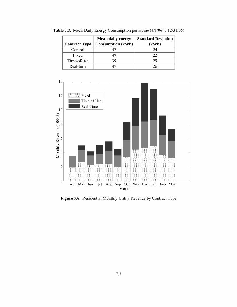
7.7
Table 7.3. Mean Daily Energy Consumption per Home (4/1/06 to 12/31/06)
Contract Type Mean daily energy
Consumption (kWh)Standard Deviation
(kWh) Control 47 24 Fixed 49 22
Time-of-use 39 29 Real-time 47 26
Apr May Jun Jul Aug Sep Oct Nov Dec Jan Feb Mar 0
2
4
6
8
10
12
14
Month
Mon
thly
Rev
enue
(100
0$)
FixedTime-of-UseReal-Time
Figure 7.6. Residential Monthly Utility Revenue by Contract Type

7.8
Apr May Jun Jul Aug Sep Oct Nov Dec Jan Feb Mar
0
1
2
3
4
5
6
7
8
9
Month
Ave
rage
Ene
rgy
Pric
e (c
ents
/kW
h)
Fixed Time-of-Use Real-Time
Figure 7.7. Residential Participant Average Monthly Energy Price by Contract Type

7.9
7.5 Effect of Wholesale Energy Price
The project adopted the MIDC wholesale price as the base of its dynamic local marginal price. This price was received by the project by subscription to a Dow Jones service. Because the price was published one day later for the hourly closing prices on the previous day, this price was necessarily projected forward and used as if it were available hourly without delay. Recall that the project’s local marginal price was roughly equivalent to this wholesale price most of the time, whenever the project virtual feeder operated well below its distribution constraint capacity.
Figure 7.8 summarizes the wholesale-price behaviors during the project. The dynamics and some longer-term trends in the wholesale price can be observed, but the MIDC wholesale price was most frequently near $50/MWh. The price is seen to shoot above $400/MWh briefly near the 270th project day, and, at the other extreme, the price did indeed fall to and remain near zero at times. The price duration curve of Figure 7.8(d) is very flat just above the price of $50/MWh. The wholesale price was significantly elevated for only about 20 hours of the year. While most project market price control was asserted to manage the local feeder constraint and thereby improve the efficient use of the local infrastructure, it should be observed that the project’s market also necessarily responded to these few hours of high wholesale price, which, one would assume, addresses more global grid-wide system efficiencies and constraints. The observed dynamic behavior of the wholesale prices, even without the additional congestion-management values added by the project’s market and local marginal price, suggest that utilities and their customers might reap market rewards by tracking even wholesale price signals if they can be communicated to utilities and customers promptly.

7.10
(a) Hourly Prices
200
Project Week
Pric
e ($
/MW
h)
1 6 11 16 21 26 31 36 41 46 51 -50
0
50
100
150
Firm PeakFirm Off-Peak
600
Pric
e ($
/MW
h)
0 5 10 15 20 25 30 35 40 45 50-100
0
100
200
300
400
500
Project Week
MIDC HourlyOlympic
(b) Daily Firm Wholesale Power Prices
Figure 7.8. MIDC Wholesale Electricity Price Behavior

7.11
(c) Wholesale Price Probability Distribution
0 100 200 300 400 500 0
0.005
0.01
0.015
0.02
0.025
0.03
0.035
Price ($/MWh)
Prob
abili
ty
(bin size = $1/MWh)
(d) Wholesale Price Duration Distribution
1 2 5 10 20 50 100 200 500 1000 2000 5000 0
100
200
300
400
500
600
Project Hours
Pric
e ($
/MW
h)
Figure 7.8 (Contd)

7.12
7.6 Residential Load Shapes
Residential participant load behavior was affected by participants’ choices of contract. The load shapes for project participants’ residences are shown in Figure 7.9, where separate figures are presented for the four seasons. “Winter” refers to January through March, “spring” refers to April through June, and so on. The figures are also separated out to show weekday (Monday through Friday) behaviors and weekend (Saturday and Sunday) behaviors. No special efforts were used to eliminate from these figures or report load behaviors for holidays.
It is no surprise that these Northwest residential loads demonstrate winter peaking with two distinct daily peaks. The largest peak occurs at about 7:00 AM, and the second, smaller peak, occurs at about 6:00 PM.
Small differences in these load shapes for the entire residential load can be seen for the behaviors of the various contract types. Time-of-use was most effective at reducing peaks for entire residential loads. Indeed, the difference in the time-of-use rate between peak and off-peak rates was a factor greater than 5 and earned a significant response. Time-of-use control, however, resulted in abrupt, not smooth, load changes during the start and end of the peak intervals, which were applied to the population at the same time, the effect of which could be detrimental. Furthermore, the fall weekend day graph shows that the improper assignment of the peak interval (people awaken later on the weekend) can perhaps exacerbate rather than reduce the peak, making it more pronounced, albeit delayed.

7.13
(a) Winter Weekday
0 3 6 9 12 15 18 210
1
2
3
4
5
6
Hour of Day
Ave
rage
Res
iden
tial D
eman
d (k
W/h
ome)
ControlFixedTime-of-Use Real-Time
(b) Winter Weekend
0 3 6 9 12 15 18 210
1
2
3
4
5
6
Hour of Day
Ave
rage
Res
iden
tial D
eman
d (k
W/h
ome)
ControlFixedTime-of-UseReal-Time
Figure 7.9. Diurnal Residential Load Shapes for each Season and Day Type by Contract Type

7.14
(c) Spring Weekday
0 3 6 9 12 15 18 210
1
2
3
4
5
6
Hour of Day
Ave
rage
Res
iden
tial D
eman
d (k
W/h
ome)
ControlFixedTime-of-UseReal-Time
(d) Spring Weekend
0 3 6 9 12 15 18 210
1
2
3
4
5
6
Hour of Day
Ave
rage
Res
iden
tial D
eman
d (k
W/h
ome)
ControlFixedTime-of-UseReal-Time
Figure 7.9 (Contd)

7.15
(e) Summer Weekday
0 3 6 9 12 15 18 210
1
2
3
4
5
6
Hour of Day
Ave
rage
Res
iden
tial D
eman
d (k
W/h
ome)
ControlFixedTime-of-UseReal-Time
(f) Summer Weekend
0 3 6 9 12 15 18 210
1
2
3
4
5
6
Hour of Day
Ave
rage
Res
iden
tial D
eman
d (k
W/h
ome)
ControlFixedTime-of-UseReal-Time
Figure 7.9 (Contd)

7.16
(g) Fall Weekday
0 3 6 9 12 15 18 210
1
2
3
4
5
6
Hour of Day
Ave
rage
Res
iden
tial D
eman
d (k
W/h
ome)
ControlFixedTime-of-UseReal-Time
(h) Fall Weekend
0 3 6 9 12 15 18 21 0
1
2
3
4
5
6
Hour of Day
Ave
rage
Res
iden
tial D
eman
d (k
W/h
ome)
Control Fixed Time-of-Use Real-Time
Figure 7.9 (Contd)

7.17
The real-time contract load behavior is perhaps smoothest. The fact that the real-time price control is active only when it is most needed implies that, on average, the real-time price control would not and did not result in the lowest average peaks. Evidence will be provided later that the real-time price control strategy was, nonetheless, effective at reducing congestion peaks when it was most important to do so.
The real-time contract group had a shifted load shape for its thermostatically controlled space conditioning that was directly responsive to market price. Figure 7.10 shows the actual and counterfactual thermostat loads for thermostatically controlled space conditioning of real-time contract homes during the most- and the least-constrained periods of feeder control. Because all participant bids for real-time price contracts were recorded when the market cleared, both the actual and counterfactual energy could be computed for each market period. The actual energy is the power cleared multiplied by the 5-minute duration of the market. The counterfactual energy is the energy that would have been used had the market cleared at the average, not the cleared, price (i.e., with a zero price deviation). Therefore, the counterfactual energy is defined as the market interval multiplied by the sum of each power that each customer would have consumed had the price not deviated, i.e., had the market cleared at the average price. The counterfactual load curves of Figure 7.10 show credible heating load behavior and also the anticipated behavior of space conditioning during the constrained fall period. However, the real-time market price induced an interesting shift of the thermostatically controlled load whether feeder supply was being constrained or not.
When demand was high and the system was constrained, the shift of real-time demand to off-peak hours was significantly larger because of the large local marginal market price differential between off-peak and peak hours. Recall that the real-time price contract tracks a daily average local marginal price and therefore allows, or even encourages, energy consumption in the early morning when daily prices are lowest. Some participants selected comfort settings that further exaggerated this shift by pre-cooling or pre-heating their homes by up to 3oF when market prices were much below average. This shift occurred on both constrained and unconstrained days. On unconstrained feeder days, price volatility moderated, and the thermostats (responding to numbers of price standard deviations above or below the average price) became increasingly sensitive to smaller diurnal price variations. While the transactive control design did not explicitly predict future price, the diurnal nature of the price itself effectively induced opportunistic pre-heating or pre-cooling more successfully than the project had anticipated. Other strategies do not use off-peak energy as effectively as real-time price-responsive demand does, and therefore, the real-time controllers used more energy during those off-peak hours when electricity happened to be a bargain.
While interesting, the energy consumption shift exhibited by these thermostats was insufficient to visibly shift the load curves for entire RTP contract homes. The heating energy cleared through the bidding process was only a fraction of what might be anticipated for the heating loads of these homes. Thermostats using “no reaction” occupancy modes, for example, did not bid and would therefore diluted the average energy consumption of the RTP thermostat population.
The only consistently measurable energy-use impact that can be observed is the energy-use reduction of time-of-use participants during peak hours. The real-time price energy reduction only occurs during actual peak conditions and cannot be easily discerned in the aggregate load shape, which includes both peak and non-peak load conditions. In contrast, the peak time-of-use price signal is applied during certain hours of a day, oblivious to whether electricity truly becomes constrained during that period.

7.18
(a) During Unconstrained Supply Conditions
(b) During Constrained Supply Conditions
0 3 6 9 12 15 18 21 0
0.50
1.00
Hour of Day
Ave
rage
Spa
ce C
ondi
tioni
ng D
eman
d (k
W)
Actual (14.2 kWh/day, 0.9 peak kW)Counterfactual (12.2 kWh/day, 0.8 peak kW)
(500-kW feeder constraint period)
0.25
0.75
0 3 6 9 12 15 18 210
0.50
1.00
Hour of Day
Ave
rage
Spa
ce C
ondi
tioni
ng D
eman
d (k
W)
Actual (10.1 kWh/day, 0.7 peak kW)Counterfactual (8.5 kWh/day, 0.4 peak kW)
(1500-kW feeder constraint period)
0.25
0.75

7.19
Figure 7.10. Real-time Market Shifting of Thermostatically Controlled Residential Load
7.7 Commercial Load Shape
Figure 6.7 shows the load shapes for the MSL buildings. The MSL buildings are office and laboratory facilities with a relatively constant load through each day. Some variation, caused by facility occupancy, was shown between weekdays and weekends. The shown load shapes were not broken down by season. Some seasonal variation would be expected, of course.
7.8 Feeder Capacity
The virtual feeder capacity constraint was varied two times throughout the project to explore the responses of residential and commercial, supply and demand, feeder resources operating under different feeder supply constraints. The feeder constraints are summarized in Table 7.4. The most interesting feeder activity was observed during late October 2006 when the feeder capacity was at its lowest value relative to total feeder demand. Figure 7.11 shows feeder demand during two such weeks.
The counterfactual demand was deduced by examining the loads’ bids. Knowing the bid strategy used to generate bids and knowing the control strategy used to manage the device load, one can deduce what the prevailing conditions were at the time the bid was generated. From this, it can be inferred whether the device would have been running were the real-time price and market feedback unavailable (i.e., if the load were responding to an immutable, average price.)
It can be seen in week 30 (Figure 7.11) that whenever the counterfactual demand exceeded the feeder capacity, the actual demand was held down for a time, either until system demand decreased or until the economic incentive to start the first distributed generating unit overcame the cost of starting it. At this time, the sum of feeder capacity and distributed generation was temporarily allowed to exceed the feeder limit. It can be seen in week 31 (Figure 7.11) that this process can result in flat demand for extended periods, with the demand tracking the available generation, rather than the other way around.
Table 7.4. Summary Application of Distribution Capacity
Dates Capacity (kW)1 Apr–22 Sep 1500 22 Sep–8 Dec 500 8 Dec–31 Mar 750

7.20
(a) During Moderately Constrained Supply Conditions
Sat Sun Mon Tue Wed Thu Fri Sat0
100
200
300
400
500
600
700
(Week #30: Oct 21 - Oct 27)
Dem
and
(kW
)
Counterfactual Feeder Limit Actual Demand
(b) During Heavily Constrained Supply Conditions
Sat Sun Mon Tue Wed Thu Fri Sat 0
200
400
600
800
1000
1200
1400
(Week #31: Oct 28 - Nov 03)
Dem
and
(kW
)
Counterfactual Feeder Limit Actual Demand
Figure 7.11. Served and Managed Distribution Load

7.21
This phenomenon can be easily explained by considering how the actual demand is determined by the real-time market. When the demand is very low, the feeder itself is the marginal energy supplier, and the local marginal price is set at the feeder’s bid price—very near the wholesale energy cost. Under these conditions, the load fluctuates while remaining below the feeder capacity, and the price remains constant, as shown in Figure 7.12(a). However, as the demand increases, the consumers become the marginal resources, and the feeder is run at capacity, as shown in (b). Under these conditions, the price fluctuates, but the load remains constant. If the demand continues to increase, then at some point, the real-time price raises high enough to start the first distributed generating unit, which then becomes the marginal supplier. This returns us to the previous condition where the price is constant, but the load fluctuates, shown in (c).
P
Q
P
Q
P
Q
P
Q
P
Q
P
Q (a) (b) (c)
Figure 7.12. How Real-time Price Can Flatten Load
It is interesting to note the decreased effectiveness of the real-time price control when severe weather conditions made demand less capable of responding to price, as was the case during week 36, shown in Figure 7.13. In this case, there were comparatively fewer satisfied loads bidding on the demand side, and this resulted in much closer tracking of the actual to counterfactual demands.
This illustrates the need to have a substantial amount and diversity of loads that can follow real-time prices under extreme weather conditions. There must remain enough satisfied load that can respond to increasingly high prices under constrained supply conditions. Indeed, the severity of the demand-response shortage can be seen when the feeder capacity was increased on Friday. Immediately after the relaxation of the feeder constraint, the load exceeded the counterfactual demand for nearly half the day until normal operating conditions were restored.

7.22
Sat Sun Mon Tue Wed Thu Fri Sat0
200
400
600
800
1000
1200
1400
(week #36 Dec 2 - Dec 8, 2006)
Dem
and
(kW
)
Counterfactual Feeder Limit Actual Demand
Figure 7.13. Distribution Operations during Critically Constrained Feeder Conditions
7.9 Project Peak-Load Reduction
One interesting figure of merit for the project is the actual reduction in peak load observed during the experiment. Figure 7.14 provides an interesting estimate of effective peak-load reduction during each of the three imposed feeder constraints. The separations between the actual and counterfactual curves become increasingly greater near the peak load (toward the left of each diagram) and for the progressively more constrained feeder operating conditions from 1500 kW (Figure 7.14(a)) to 500 kW (Figure 7.14(c)). A plateau occurs in the actual load curves at each respective constraint magnitude, where load is actively being deferred to manage the feeder constraint. The widths of these plateaus represent the duration for which the loads acted as marginal market resources reducing capacity and holding the local marginal price constant near the wholesale price. Operation to the left of these plateaus eventually required that distributed generators be included into the generation mix. Other plateaus appear where the loads are perhaps managed as marginal resources, again to avoid calling upon second or third distributed generators to run. The reduction of peak load appears to have been about 5 percent for the 750-kW constraint period and up to 20 percent for the 500-kW constraint period. According to these load-duration diagrams, there was about a 5 percent increase in “peak” load for the 1500-kW unconstrained period, a result which the project cannot yet explain.

7.23
(a) 1500-kW Feeder Capacity (Summer)
10-5 10-4 10-3 10-2 10-1 100 0
100
200
300
400
500
600
700
Fraction of Hours
Load
(kW
)
ActualCounterfactual
(b) 750-kW Feeder Capacity (Winter)
10-5 10-4 10-3 10-2 10-1 1000
200
400
600
800
1000
1200
Fraction of Hours
Load
(kW
)
ActualCounterfactual
Figure 7.14. Feeder Load Duration Curves

7.24
(c) 500-kW Feeder Capacity (Fall)
10-5 10-4 10-3 10-2 10-1 1000
200
400
600
800
1000
1200
Fraction of Hours
Load
(kW
)
ActualCounterfactual
Figure 7.14 (Contd)
The power flowing through the feeder distribution line divided by how much power would have flowed through the line had the demand response and distributed generators not been operating will be called peak reduction. The project estimated the peak reduction achieved in the entire feeder by the project’s control of a limited number of the residential, commercial, and municipal resources on the feeder. The summary for these peak reduction estimates is found in Table 7.5. The project achieved impressive 19 percent and almost 30 percent average peak reductions for the 750- and 500-kW constraints, respectively. No peak reduction is estimated for the remaining 1500-kW feeder constraint condition, which never experienced challenging feeder congestion conditions and needed no peak management.
Figure 7.15 shows the weekly peak reductions when the project constrained the feeder. The counterfactual (“would have been”) load was calculated by using the buy bids to compute what the loads would have consumed had the market cleared at the average daily price with no variance. Since no distributed generators would have operated for the counterfactual, their operation was always excluded from the counterfactual projection. During the other two more constrained periods, peak reductions for many weeks greatly exceeded the reported averages.

7.25
Table 7.5. Average Peak Reduction during Constrained Project Periods
Period Constraint Mean Reduction Sigmafall 500 kW 29.7% 18.7%
winter 750 kW 19.0% 9.7%
Project WeekFeeder Capacity Limit500 kW: mean=29.69% ( σ =18.65%)750 kW: mean=19.02% ( σ =9.72%)
0 5 10 15 20 25 30 35 40 45 50 0
10
20
30
40
50
60
70
Wee
kly
Peak
Red
uctio
n (%
)
500
1250
750
1000
1500
250
Feed
er C
apac
ity (k
W)
1750
Figure 7.15. Peak Reduction and Imposed Feeder Capacities during the Project
One important result for the project was its successful management of feeder power constraints under peak load conditions, as is shown in Figure 7.16. Whenever the feeder became constrained, additional supply was offered to, and in some cases delivered to, the load by distributed generators from within the feeder. The capacity of these distributed generators was seamlessly offered and cleared through the project’s market. For the 500-kW feeder, the peak total demand bid capacity was 1,264 kW, and the peak cleared supply was 901 kW. For the 750-kW feeder, the peak total demand bid capacity was 1,280 kW, and the peak cleared supply was 1,138 kW. For the 1500-kW feeder, the peak demand bid and peak cleared supply were both 649 kW. Note that the virtual feeder itself was successfully managed to remain under its imposed distribution capacity limit (i.e., 500, 750, or 1500 kW) for all but one brief interval. In only one instance (under the 500-kW feeder) did the market fail to clear because the total supply offer was less than the portion of the demand bid from unresponsive, uncontrolled loads. During that single 5-minute period, the feeder supplied 520 kW, which was 20 kW (0.2 percent) over its limit.

7.26
(a) 500-kW Feeder Capacity (Fall)
10-5 10-4 10-3 10-2 10-1 1000
200
400
600
800
1000
1200
Fraction of Hours
Total Demand Bid Cleared Total Supply Feeder Supply
Supp
ly (k
W)
(b) 750 kW Feeder Capacity (Winter)
10-5 10-4 10-3 10-2 10-1 100 0
200
400
600
800
1000
1200
1400
Fraction of Hours
Total Demand BidCleared Total SupplyFeeder Supply
Supp
ly (k
W)
Figure 7.16. Supply Duration Curves

7.27
(c) 1500-kW Feeder Capacity (Summer)
10-5 10-4 10-3 10-2 10-1 100 0
100
200
300
400
500
600
700
Fraction of Hours
Total Demand BidCleared Total SupplyFeeder Supply
Supp
ly (k
W)
Note: feeder supply and cleared supply are the same.
Figure 7.16 (Contd)
7.10 Consumer Surplus
Consumer surplus is that excess portion of satisfied load bids that exceeds the eventual closing market price in a two-sided market. In this sense, it can be represented by the shaded region in the market closing diagram of Figure 7.17. It represents the bids from consumers that were “left on the table” unclaimed by the utility. The consumer surplus is the basis of an argument for price differentiation. The utility can capture more revenue if it can differentiate its service and price accordingly for supplying the highest bidding customers who consistently bid at the top left of the shown load curve.
The project examined the consumer surplus for both residential and commercial real-time participants. The residential consumer surplus was very small compared to the commercial consumer surplus, as is shown in Figure 7.18. This result was unexpected given that commercial loads are often given a discounted differentiated price, the opposite of what is suggested here.
The discrepancy between consumer surpluses of the commercial and residential load populations can be explained as follows: in fact, available resources for demand response at the commercial level were small compared to total demand of commercial buildings. The control system used the real-time price market signal to control the variable air volume dampers of commercial HVAC. From December through March, price also controlled the commercial electric boiler. However, the generating units adjacent to the

7.28
commercial building could not be run on-grid, forcing those generator units to bid on the demand-side, and only for the displaceable load value of the served building load. The price of those distributed generator load bids was for the generator start-up with a minimum runtime of 30 minutes, which was typically very much greater than the clearing price of the market. This suggests that the presence of the non-synchronous generators on the load side of the market artificially inflated the apparent bids of the commercial load entities and thus the magnitude of the commercial consumer surplus.
Capacity
Price/Cost
Generation
Load
Consumer Surplus
Figure 7.17. Definition of Consumer Surplus on a Market Closing Diagram
It should also be stated that commercial entities have more market clout than do residential customers and might have superior opportunities to change from one electricity supplier to another. This additional market force might entice suppliers to hold electricity prices low, even if commercial consumer surplus is shown to be high.
The consumer surplus expressed by hour of day and seasonally, as shown in Figure 7.19, reveals the degree to which consumer surplus varies during peak demand periods. Seasonally, the load and resource market lines intersect more steeply during fall and winter, thus increasing the consumer surplus during much of the day. However, during the peak heating hours, the consumer surplus diminishes with higher closing prices. This observation confirms that the real-time price control does indeed capture the economic value of demand for the utility during peak periods.

7.29
Apr May Jun Jul Aug Sep Oct Nov Dec Jan Feb Mar
0
500
1000
1500
2000
2500
3000
Month
Con
sum
er S
urpl
us ($
thou
sand
)
Commercial Residential
Figure 7.18. Consumer Surplus by Month
0 5 10 15 20 25
140
160
180
200
220
240
260
280
300
320
Hour of Day
Con
sum
er S
urpl
us ($
1000
)
Winter SpringSummerFall
Figure 7.19. Seasonal Consumer Surplus by Hour of Day

7.30
7.11 Production Dispatch
Distributed generating units were dispatched based on whether their bids cleared the market. The peak distributed generation dispatch in December (Figure 7.20(a)) is most likely due to the extreme shortage of wholesale power imposed on the project’s feeder until December 8. After that date, the feeder capacity was increased from 500 to 750 kW, and thus less generation dispatch was required. The peak distributed generation dispatch hour was around 8:00 AM, with a smaller peak around 6:00 PM (Figure 7.20(b)). This observation coincides well with the demand load shapes presented earlier.
7.12 Contract Type Mixtures for Achieving Desirable Risk / Benefit Ratios
An innovative analysis approach was developed by PNNL and applied to the project market results. In this approach, analysis tools common for the selection of asset portfolios are applied to mixes of price contract types.
7.12.1 Efficient Frontiers
The concept of efficient frontiers was introduced in 1952 by Nobel Prize winner Harry Markowitz (1952) as part of the Capital Asset Pricing Model (CAPM) for portfolio theory. The principle is that combining several stocks into a portfolio can decrease the overall risk below that of any individual stock while still attaining a comparable return.
Figure 7.21 depicts this idea. The area in green shows all possible ways (weightings) to combine a group of stocks to make up a portfolio. The top leading edge of this diagram, the efficient frontier, provides the optimal combinations (weightings) of these stocks. This top and left boundary provides the highest return for the lowest risks. No person should wish to invest in a portfolio below the efficient frontier. From below the efficient frontier, the return can always be increased without increasing the risk, or analogously, decrease the risk, for the same return.
For the stock market, risk is defined as the volatility of a stock. In its truest form, Figure 7.21 simply shows that any number of normal random variable distributions combine to form a unique random variable distribution. The optimal way to combine any set of normal random variables can be determined.
The project poses the question, “Given several types of markets that can be offered to customers, what is the optimal combination of these markets to offer?” The Olympic Peninsula Project compared three principle market types: a fixed-price contract, a time-of-use contract, and a real-time price contract. Data obtained over a 1-year period make up the random variables that are needed to perform efficient frontier calculations.
The efficient frontier diagrams for contract types do not necessarily have the same implications as they do in stock analysis. For example, a point on the efficient frontier in stock analysis is by definition considered “good”; however, the efficient frontier for contract type analyses may be good or bad. This analysis does not provide conclusive answers, but rather it provides a rich mechanism to evaluate the consequences of any given contract type mix. Whether a mix is good or bad depends upon the objectives of the utility.

7.31
Apr Ju Oct Nov Dec Jan Feb Mar
0
2000
4000
6000
8000
10000
12000
14000
16000
18000
Month
DG
Dis
patc
hed
(kW
h)
(a) Dispatched Distributed Generation by Month
1 2 3 4 5 6 7 8 9 1011 12 13 1415 1617 1819 2021 22 23 24
0
1000
2000
3000
4000
5000
6000
7000
Hour of Day
DG
Dis
patc
hed
(kW
h)
(b) Dispatched Distributed Generation by Hour of Day
Figure 7.20. Distributed Generation Dispatch

7.32
Figure 7.21. Efficient Frontier and Other Portfolio Weightings
7.12.2 Combining Distributions
Consider two normal distribution curves, each completely defined by its mean and standard deviation. Figure 7.22 shows these two curves (bold blue). Remember, these two curves represent two different sets of data. For example, the first curve might represent income from selling only wheat, the second, only barley. What income should be expected by selling both wheat and barley? The green normal distribution functions result. There are many of these curves, each representing a different mix of wheat and barley. Together, all these curves represent all possible income levels obtainable by selling different combinations of wheat and barley.
It might be assumed that the mean value of each curve would simply follow a relatively straight line between the two curves, but as can be seen, that does not happen. More is going on. An efficient frontier has been created. Mathematically, this is simply combining the two probability density functions together in different proportions.

7.33
0 1 2 3 4 5 60
0.5
1
1.5
2
2.5
Prob
abili
ty
Value
Normal Distribution #1
(wheat)
Normal Distribution #2 (barley)
Normal Distribution Combinations of #1 and #2
Figure 7.22. Two Pure Distributions (Blue) and Distributions for Mixes of the Two (Green)
Figure 7.23 shows another way of viewing this same result. What mixture of wheat and barley should be sold given that the income (mean) and variability in income (standard deviation) of all possible proportions of wheat and barley are known? If the only goal is to increase income, then all of the barley should be sold. But what about the variability of the income? This may also be important if regular proceeds from sales are needed to support operations. If, however, this is not important, then it seems clear that Barley is the way to go.
For argument’s sake, let’s assume that the income stream is important, so it is desirable to have as consistent an income as possible. A person would be willing to sacrifice a little profit to make this happen. In this case, the optimal mix of wheat and barley occurs at mean 2.6 and standard deviation near 0.165. Anywhere between this point and point #2 (all barley) would be the efficient frontier, which have been denoted as small circles on this graph. It would be necessary to never drop below this optimal point, however, because then a decrease in income would accompany the variability of income.
What if wheat were sold exclusively? Given these observations, by selling a little barley along with the wheat, the income would both increase and become more stable.

7.34
Figure 7.23. Efficient Frontier Mixtures of Two Pure Distributions
7.12.3 Electric Power Markets
Now we will leave the examples of wheat and barley and consider the electric power utility industry. In the Olympic Peninsula Project, there were three types of residential contracts offered to consumers of electric power: fixed price, time-of-use, and the real-time price.
Figure 7.24 was created from the peak energy data measured over the duration of the project. Only at the times of the year and the day when energy consumption was high were data used for this analysis. Specifically, the time of year from November 1 to December 8, 2006, and the hours of the day from 6 to 9 AM and from 6 to 9 PM were used. These data represent the times when the electric power system was at its highest capacity, and therefore they represent the best time to look at how effectively the different project contract types influenced the system capacity.
An efficient frontier analysis was performed. The shaded surface represents all possible proportions of combining the three contract types. The three sharp points at the ends of the shaded regions represent the three pure contract types. For example, the word “fixed” appears near the coordinate (1.04, 1.075). As one moves away from the corner points in the shaded region, three contact types start mixing together. The Olympic Peninsula Project itself had a mixture of roughly 1/3 of each contract type, represented on this figure by a red dot.
If a utility wishes to reduce its peak energy use during its times of high capacity, Figure 7.24 suggests the utility should select a contract mix as low as possible on the peak energy axis. This point happens to

7.35
correspond to a 100 percent time-of-use contract assignment for this project data. It might be assumed that the utility would want the variability also to be low. However, once the peak is low enough, the utility might want the customers to further be responsive—to change their energy use as a result of price signals. This implies the utility might actually desire more variability.
Figure 7.24. Peak Energy Use for Season and Time of Day for the Duration of the Project
By itself, one efficient frontier graph is easily enough interpreted and might result in a clear suggestion of which mix should be sought, as was the case above. However, efficient frontier graphs can be drawn for other parameters, and the optimum mixture of contract types from one efficient frontier graph and a utility’s objectives for that variable might not at all optimize the utility’s objectives for another variable.
Consider another variable and its efficient frontier graph. Gross margin is defined as the revenue generated by the sale of electricity, minus the cost of that electricity. It does not include costs of infrastructure, labor, taxes, overheads, or other fixed costs. It simply gives an early preview of what profits might look like. Omitting these other fixed charges helps keep this financial metric relevant to a broad range of companies, all of which can add back in their own unique fixed charges. Unlike the previous analysis that looked only at peak periods of electricity use, this gross-margin analysis uses data for the residential homes for the entire project year, 24 hours per day and 7 days per week. Keep in mind that these data are simply different parameters from this same project.

7.36
Figure 7.25 is the efficient frontier graph for gross margin for the duration of the Olympic Peninsula Project. There are still three extreme locations, but the pure fixed contract point is somewhat hidden behind the surface. Both this point and the project’s gross margin are emphasized by red dots on the figure. Whereas mixtures heavy in time-of-use contracts minimized energy peaks in the previous analysis and might be preferred, time-of-use contracts also minimize gross margin and would not be preferred in this analysis. This is a clear example of how utility objectives might create contradictions during efficient frontier analyses of different parameters.
Regardless, the adoption of this analysis approach shows great promise for utility selection of contract mixes. This approach clarifies the tradeoffs in satisfying utility objectives and acceptable risk, or variability, of tradeoffs.
Figure 7.25. Gross Margin of Utility per Hour per Residential Customer for the Project Year

8.1
8.0 Perspectives
The Olympic Peninsula was a collaborative project requiring the active or passive participation and cooperation of many. Representatives from residential participants and utilities were invited to submit perspective statements at the conclusion of this project. These documents are reprinted here, attributed to the contributors who offered the project such unique and useful insights.
8.1 Utility Perspective
The project gathered perspective statements received from City of Port Angeles Public Works and Utilities, from PUD #1 of Clallam County, and from BPA.
8.1.1 City of Port Angeles Public Works Perspective
The management of the City of Port Angeles Public Works and Utilities provided the following perspectives on their involvement as a field site host for the Olympic Peninsula Project.
“Offered the opportunity to participate in a technology based load management experiment, the City of Port Angeles (City) was pleased to participate in the U.S. Department of Energy’s Olympic Peninsula Project. The City’s role in this demonstration project was limited to that of a host utility, it provided PNNL with a residential customer base to conduct their experiment on and provided the City’s customers the opportunity to participate in an experiment of national significance. Through its participation in the experiment, the City anticipates gaining some insight into the practicality, availability and customer acceptance of a technology based load management option.
“The Olympic Peninsula Project involved the deployment of an Invensys Controls energy management system (EMS) in the homes of volunteer participants in two electric utility service territories on the North Olympic Peninsula. The EMS controlled the electric water heater and the central heating system thermostat of each house participating in the demonstration project. Customers could access control of the water heater and the thermostat through the Invensys GoodWattsTM Energy Management Web site and program the appliances’ operation during the demonstration project. A variety of energy use reports for the period of the experiment were also accessible to participants for all of the appliances and the whole house meter. PNNL could also access the water heaters and thermostats and consumption data via the Invensys GoodWatts Energy Management Web site. PNNL could also override the customers programmed settings and observe responses to the overrides.
“Grid Friendly appliance (GFA) clothes dryers were also installed in fifty (50) City demonstration project homes. The GFA clothes dryer provides display panel signals to communicate to the customer that the utility electric grid may be stressed due to high demand. PNNL could also manipulate the GFA display signal simulating utility grid stress and observe customer responses to the signals.
“Participating customers selected and were assigned to one of four different experimental contract types—control, fixed, time-of-use, or real-time pricing. Depending on how well customers managed the energy consumption of these appliances they were periodically financially rewarded by the project. PNNL will also administer an exit survey to help assess customer acceptance of the technology. PNNL

8.2
collected experiment data and will publish a report on the performance of the appliances and customer responses.
“As a host utility, the City was tasked with assisting PNNL in recruitment of experiment participants (test subjects). One complication encountered during recruitment was in communicating the nature of the experiment. Many of the City’s customers that expressed early interest in the experiment assumed this was an energy conservation project and had some difficulty making the connection to load management. Some of the initial volunteers were not willing to give up absolute control of their thermostat or water heater. Many of the experiment participants were older customers who were transplants from other regions of the country and had some experience with time-of-use electric rates and the benefits of load management. Unfortunately, the City did not have many younger utility customers with larger households participate in the experiment. Participant recruitment goals were not easily met and the recruitment period lasted longer than expected despite the possibility of financial rewards.
“As a host utility the City was also concerned with the ease of installation and customer satisfaction with the installation of the GridWise equipment by local contractors. Some communication problems resulted in a few customer complaints involving scheduled installation times and unannounced cancellations. Other issues concerning installation were related to compatibility of the home to the experiment. Common problems encountered were incompatible heating systems (systems without a single thermostatic control), incompatible Internet access (not broadband or not always connected), and the physical location of utility electric meter and appliances involved in the experiment (proximity of load control modules (LCM) within wireless signal range of each other). Some of the problems were resolved through the ingenuity of the equipment installer. Some of the initial experiment volunteers were not able to participate because certain issues could not be resolved. Overall customer complaints were at a minimal and most of the initial participants remained in the experiment until its completion. However, this particular technology was limited to broadband Internet access, common in the City’s service territory but not ubiquitous.
“The City also provided the service of the revenue electric meter change out to the Invensys meter used in the experiment. With the exception of a few field decisions made by the City’s meter-man all meters were installed. It was discovered that the Invensys meter is limited in its application to single-phase 200-amp service meter bases, the most common residential meter base in the City’s service territory. However, there are a few residences that have three-phase service and could be precluded from participating in a similar utility wide technology based load management program.
“The City also participated in weekly group conference calls with representatives from PNNL, BPA, Invensys, IBM, Whirlpool, Clallam County PUD, PacifiCorp, PGE, and PM&A. The conference calls discussed the progress of the experiment and issues of concern for the various partners. Initial conference calls dealt mainly with recruitment issues and the technicalities of the compatibility of various components of the experiment. These early conference calls provided some insight into the technologies and the work involved in coordinating compatibility of the appliances, LCMs and equipment communication issues. As the project progressed to the implementation stage, discussions turned to experiment participants’ understanding and use of the EMS. These discussions made it clear that customer education was as important to the success of the load management experiment as was the technology.

8.3
“The City is grateful for the opportunity to participate in the Olympic Peninsula Project and looks forward to the report to be delivered by PNNL.”
8.1.2 PUD #1 of Clallam County Perspective
The following perspective article was contributed by O. Mattias Järvegren, Utility Services Advisor for PUD #1 of Clallam County (Clallam PUD). Clallam PUD hosted the project in and near Sequim, Washington.
“Clallam PUD is a small utility located on the westernmost tip of the continental United States. It has since its earliest days been striving to provide low cost, reliable electrical service to its mainly rural customers. In 2001 Clallam PUD began to develop a fiber optic based telecommunications network to support operation and management of its electric distribution system. Clallam PUD believed that the future of an efficient electric distribution system would include an intelligent communications network, coordinating the operation of the electric distribution system with its customers’ ‘end use’ of energy.
“When PNNL contacted Clallam PUD inquiring if the utility would be interested in participating in the Olympic Peninsula Project, Clallam PUD was very excited to participate. The project offered Clallam PUD the opportunity to participate in a cutting edge experimental program where it could explore the opportunity to utilize a broadband telecommunications network to assist electric power operations. The Clallam PUD Commissioners thought that to better explore opportunities made available from technological development, Clallam PUD would take an active role in the pilot implementation of the project.
“Clallam PUD’s level of participation was originally limited to allowing PNNL to ask Clallam PUD’s customers to participate in the program, as well as doing the installation of the revenue electrical meter that was installed on each of the participating residences. In all 65 of Clallam PUD’s residential customers signed up to participate in the project. When PNNL requested assistants to identify a willing industrial participant, Clallam PUD offered to include one of its nine water districts, the Clallam Bay / Sekiu water district. The PNNL control equipment was installed on the pumps at the Clallam Bay / Sekiu water district’s two pump stations at Clallam Bay and at Hoko-Ozette.
“As a host to the program Clallam PUD was very excited to be able to include the two pumping stations in the project. However, as the project moved into its implementation phase it immediately became clear that the pump operator did not share the enthusiasm for the program. The pump operator did not like the idea of giving up local control of the pumps; an opinion that, in hind sight, is not very surprising. The pump operators were mainly concerned that the control equipment might not be programmed in such a way as to ensure the maintenance of adequate water reservoir levels. Through the project controls, the pumps would be set to respond to price signals. The pump operators did not feel that the project controls would ensure adequate water levels in the reservoir.
“To address the concerns of the pump operator, a series of telephone meetings was set up between PNNL and Clallam PUD staff. PNNL went to great length to explain to the Clallam PUD water department and the pump operator the scope and purpose of the project, and after the first of the telephone meetings a control strategy was devised that satisfied the needs of both Clallam PUD Water Department as well as PNNL.

8.4
“The project controls were set to have full control of the pumping station as long as the water levels were maintained within 3 feet of a full reservoir. Once the water level dropped below that point, the project controls would no longer place bids to curtail the pump operations. This ensured that the pumps could play an active role as an industrial load in the project, as well as keep the water levels at an acceptable level due to the operator’s safety concerns. The control equipment on the pumping stations was programmed to place electric market bids that were inversely proportional to the reservoir of each pump station. In the event that electrical market price exceeded the pump bid, the pump controls would issue a control signal that would curtail operations of the pump, releasing power resources that were used by the pump at the time of operation. The pump controllers were programmed such that each pump command signal was immediately accompanied by an ‘On Delay’ control signal that was sent to ensure that the pump would not shut off until after at least 5 minutes. Following the release of each command signal an “Off Delay” signal was sent to prevent another curtailment from occurring within 15 minutes from the release of the last curtailment. These delay signals were incorporated to ensure that the pump controls would not affect the useful life of the pumps by short cycling the pump excessively. Subsequent phone meetings between Clallam PUD staff and PNNL program management focused primarily on ensuring that the pump controls were operating as stated and that the concerns of the pump operators had been satisfied by the agreed upon control strategies.
“One of the clearest lessons from the program has been the importance to educate all program participants and of thoroughly evaluating the loads incorporated in a load management program. The resistance from the pump operators at Clallam Bay and Hoko-Ozette was not exceptionally hard to overcome. This is in part due to the fact that Clallam PUD’s Utility Services Department acted as an ombudsman between the Clallam PUD’s Water department and PNNL. Working through another Clallam PUD Department made the Water Department more comfortable giving up some control of the pump station. The situation does highlight the importance of having an advocate from within the participating organization. Had there not been an internal advocate at Clallam PUD to encourage and facilitate program support, the pump controls might very well have been disabled by the pump station operator very early in the program. From PNNL’s side, the issues brought forth by the pump operators were addressed thoroughly and clearly through the several phone meetings, where PNNL allowed the Clallam PUD Water Department to assist in determining what controls strategies would be appropriate for the pump stations. When considering a potential future program like GridWise, an honest and clear dialog between the utility and its customers will be an essential component of a successful implementation of the program. Both parties need to have a clear understanding of what each others goals and concerns are so that the load management program can be implemented with mutual benefit of the involved parties.
“PUD #1 of Clallam County is thoroughly satisfied with the expertise and professionalism of the staff at Pacific National Laboratories and is very grateful to have had the opportunity to be able to participate in the Olympic Peninsula Project.”
8.1.3 Bonneville Power Administration Perspective
Preston Michie, a consultant, provided the following insights gained from BPA’s point-of-view as a collaborator in the Olympic Peninsula Project.

8.5
“BPA agreed to join this study to assess the efficacy of using centralized Internet based technology and Grid Friendly appliance controllers installed in water heaters. This study is an adjunct to BPA’s involvement in a similar program in Ashland, Oregon. The additional feature of particular interest to BPA in the current study, in addition to testing GFA technology in water heaters, is the linkage of consumers to market prices through their choice of virtual service contracts with fixed, critical peak pricing, or real-time pricing.
“While a robust real-time market does not yet exist in the Pacific Northwest, it was useful to BPA to engage in early stage assessments of technologies that linked consumer response to wholesale price signals to manage system problems. This was particularly so on the Olympic Peninsula where BPA seriously considered installing demand response devices on the Peninsula to defer transmission upgrades.
“Thus, BPA was interested in consumer response to this technology in a more disperse area, the efficacy of the interface between consumer and wholesale markets, the impact of consumer choice of service contracts in exchange for the opportunity to get paid to respond to system conditions, and the efficacy of GFA technology to manage underfrequency events.
“From these perspectives the program was a success because it assessed these four areas of interest and because it added to BPA’s knowledge base. BPA expected the centralized Internet based technology to work. However, it was less certain that consumers would respond favorably to service contract choices and stick to their choice given volatile market prices. Similarly, BPA expected the GFA devices to work. This part of the study essentially validated what BPA thought would be the case. BPA saw value in demonstrating that these automatic responding devices work in the field as intended.
“What would it take for these technologies to be of serious interest to BPA? In a nutshell: scale, programmability, reliability, cost, and cost recovery. Scale is an issue for a system as large as BPA’s. Unless the combined magnitude of centrally control demand response approaches several hundred MW, it is too small to provide significant services to help BPA manage frequency effectively or contribute significantly to system reliability. However, local conditions may favor installation of significantly smaller scale GridWise devices that would provide local benefits such as relieving local congestion, deferring capital additions, managing voltage, etc.
“The ability to reprogram response is potentially valuable because under some underfrequency events it is desirable not to trigger load reductions automatically. Indeed, it may be best to increase load in these instances to preserve reliability. The ability to change response parameters depending on the nature of the system condition would be a valuable feature.
“While these technologies are very interesting, BPA is aware of the difficulties of gearing up machinery to implement a major program to produce significant amounts of demand response—and sustain it over time—where the incremental addition at each site may be modest, meaning a few hundred watts. Costs of scaling up remain a concern.
“There is a dearth of trained technicians, a lack of marketing experts and materials, and no sales force. There is no distribution system in place. There are no standard contracts approved by utility commissions or other regulators. There is no mechanism to finance or insure the program. The level of public awareness is low. There is no system in place to handle billing, customer complaints, or make repairs.

8.6
“If each home could reliably provide about 1 kW of demand response during heavy load hours, one would have to wire up tens of thousands of homes to provide significant demand response—assuming perfect consumer response, no degradation in performance, and a zero failure rate over time. A large scale program could easily require an investment of tens of millions per year for several years. There would likely be significant O&M costs to address inevitable problems in keeping these systems working properly. Overhead may be high to manage a large force of contractors at work over a wide geographic area.
“A failure rate over five years from all causes (people forget to turn on their computers; they get bored; they sell their homes; replace their appliances; get annoyed with reduced amenities; the system experiences non-zero failure from faulty equipment, etc.) of just 5% translates into an additional cost that may be several million dollars over the life of the program. No one understands the ‘shelf-life’ of this technology. What if the technology is obsolete in five years?
“Sustainability is a concern. It is not clear how performance will degrade over time either because various components of the hardware or software systems fail or because consumers lose interest. At some point the rate of loss of participants might limit the potential to increase scale without a significant investment in marketing these technologies because the ‘early adopter’ market has been saturated, consumer resistance stiffens, and the penetration rate slows.
“While there is potential value in having self reacting and programmable load response, there is concern that the system will degrade for various reasons more rapidly than expected. Actually, the bigger concern may be simply that because the rate of degradation is unknown, redundant systems must be in place until degradation over time is well understood.
“The demand response itself is subject to outages when local power or internet service goes out and computers no longer work, which may seem like a modest event, but from a system perspective, the system capability to respond to an underfrequency event or other emergency is reduced when this happens.
“Like any other significant utility program, who should pay for these technologies is not an easy question to answer. Obviously the technology benefits control area operators by increasing their flexibility to respond to emergencies (particularly if programmability is an added feature), particularly where the response is automatic, local, and fast. Utilities may be able to reduce capital investment in system upgrades to maintain reliability. But the consumer also benefits in the form of a reduced bill from ‘peak shaving.’
“Independent power producers and their customers benefit from a ‘softer’ grid and potentially from the ability to contract with developers of GridWise technologies to provide ancillary, wind integration, imbalance energy, redispatch and other services, especially when coupled with distributed generators located throughout the system.
“It is not clear whether the technology should be mandated by utility commissions and other regulators or whether deployment should be left to the market. Is this technology financeable, meaning will investors and bankers provide needed capital? At what cost? There is no uniform platform for appliance manufacturers to deploy to make “super smart” appliances universally compatible with one another and with interface technology. It is not clear how improvements in technology will be distributed.

8.7
“In sum, while these technologies are potentially valuable additions to the tools with which to manage reliability and provide other valuable services, many questions related to scalability and public policy remain. While BPA is confident that the challenges of scale can be solved, BPA believes it is important to better understand issues of scale before committing to an extensive program to invest in these technologies.
“Nevertheless, based in part on the success of the Ashland and Olympic Peninsula studies, BPA intends to continue to support the development of centralized demand response technologies. It intends to work closely with the National Labs, regional utilities, and others in supporting the development of these and related promising technologies.”
8.2 System Integrator Perspective
IBM provided the middleware solution by which distributed project resources participated in the real-time energy market.
8.2.1 IBM Perspective
The following article was submitted by authors Ron Ambrosio and Mark Yao of the T. J. Watson Research Center, IBM. Ron Ambrosio is IBM’s Global Research Energy & Utilities Industry Leader, and is a member of the U.S. Dept. of Energy GridWise Architecture Council. His research areas include embedded systems and distributed application environments, with particular emphasis on Cyber-Physical Business Systems or the integration of sensor and control-system environments with business process environments. Mark Yao is a member of the Wireless and Embedded Technology Practice of the Application Innovation Services group. His specialties include embedded control systems, distributed computing and middleware services, and the integration of e-business processes with physical control systems. For the past four years he has worked on the Internet-scale Control Systems (iCS) project at the T. J. Watson Research Center.
“The most innovative functionality in the Olympic Peninsula Project is the implementation of the market-based control of demand response assets in the real-time price contract homes. The experiment requires each programmable thermostat to understand how to create a buy bid into the real-time market based on participant comfort goals, the current state of the device (e.g., the temperature in the home), and the current trends of the market (note that the water heaters are not bidding into the market – they are using an open-loop control scheme in which they only respond to price signals from the market). Both the thermostats and water heaters then have to respond appropriately to the clearing price generated every five minutes before the cycle starts again (the distributed generator assets are also bidding and responding, but using a different software and communication approach, so they are not discussed here).
“The design and implementation of this part of the system is based on a prototype event-based programming framework developed at IBM’s T. J. Watson Research Center called Internet-scale Control Systems (iCS). iCS is an example of what is currently emerging in the academic and research community under the category of cyber-physical systems, reflecting the increasing importance of monitoring and managing the physical world in a much richer and more detailed fashion. The physical world, in this case, is the electric grid and its associated end-use loads (such as heating and air conditioning systems).

8.8
“In practical applications, there is an additional aspect that needs to be reflected – cyber-physical systems will almost always operate within the context of some business environment. In the Olympic Peninsula Project, the business environment is reflected in the use of a market-based control scheme and the need for devices to be virtually augmented with business domain awareness – they need to bid into the market and react to clearing events. For this reason, IBM Research is focusing on an expanded scope of investigation referred to as Cyber-Physical Business (CPB) Systems, which includes both discrete event-based and continuous data stream-based systems. The objective is to define a middleware framework that addresses solutions such as Intelligent Utility Networks, which involve the integration of the physical operations domain with the business domain, dealing with the challenges of a highly distributed and heterogeneous environment, and also reflecting the time-dependent nature of such integrated solutions.
“By using a loosely coupled event-programming approach, with a very simple programming model, iCS enabled all the components of the system to be abstracted and represented as simple sensor, actuator, or control objects in the market-control application, from the market itself all the way down to the heating element relays and load monitoring sensors on the water heaters. The additional market-awareness and bidding and response algorithms were added in the middleware framework without modification of the devices themselves, essentially creating new, more intelligent virtual devices from the perspective of the market. This also allowed the design to be easily adapted during development in response to adjustments in requirements or other issues that surfaced. In addition, iCS enabled the overall market-control application to be structured as a layered set of hierarchical control loops linked together through the event communication model.
“An additional benefit of using a loosely coupled event-based approach is the level of resiliency it affords. The system was implemented such that any loss of communication or failure in the market clearing signal results in devices falling into a safe degraded mode. Operations continue in a less-than-optimal mode, but there is no catastrophic failure. Once the problem is resolved, the system returns to its optimal state.
“Halfway through its one year of operation, the Olympic Peninsula Project is just entering the region’s winter electricity-constraint season. Several cold periods have already occurred, and the real-time market system is operating as designed, limiting total load on the virtual distribution feeder to the configured capacity through price-based demand response management, and dispatching distributed generators when the market price for electricity meets the sell bids. When no constraints exist, the market price is stable and in the expected range. In terms of real-time price contract performance it appears there is a more optimal shifting of load than with the time-of-use contracts.
“Another intermediate observation is that the fixed price contract homes sometimes shifted more load than the time-of-use homes. That may be an artifact of the small sample size and the individual participants involved, but it is still an important result in that it indicates customers will respond manually to well-designed visual indicators and information sources about their consumption and cost.
“An additional positive indicator has surfaced as a result of extending the project end date: most of the residential participants asked to continue, presumably because they have been satisfied that the system is having a positive impact on their electricity consumption, and to some extent on their overall electricity cost.
“The Olympic Peninsula Project has already succeeded in a number of dimensions, from demonstrating the effectiveness of a Cyber-Physical Business System approach in designing such

8.9
solutions, to generating a great deal of interest and awareness in the optimal management of combined demand response and distributed generation in dealing with a variety of issues in electric grid operations. The goal of using this project as both an experiment and an educational tool is already starting to be realized.
“The project also represents an important milestone in the realization of the GridWise vision of an Intelligent Utility Network through its integration of utility and customer assets, leveraging advanced information technologies and bridging the operations and business domains of the utility environment. Further, it has been an extremely successful collaboration of industry and public organizations, including equipment and information technology vendors, investor owned utilities, public utility districts, and the Department of Energy’s national laboratory system.”
8.3 Equipment Manufacturer Perspective
Whirlpool Corporation built visual and audible notification into the project clothes dryers that were installed in homes. While Whirlpool’s main project focus was the Grid Friendly Appliance Project (Hammerstrom 2007), they also provided “Pr” and “En” indications on dryer panels and audible alarms to announce to participants when prices had become unusually high or when other grid emergencies existed.
8.3.1 Whirlpool Perspective
Gale R. Horst, Lead Engineer for the Corporate Innovation Technology group at Whirlpool Corporation provided this appliance manufacturer’s perspective article.
“In addition to the Grid Friendly focus, one third of the project dryers were targeted to be installed into a region where a real-time price contract test would be conducted in the same homes. For the economic experiment these homes received pricing signals via the communication and measuring equipment. Since this equipment would be connected to the dryers for measuring the experiment, Whirlpool volunteered to enable the dryer controls with an additional feature. When a high price signal is sent to the homes, the dryer can display a ‘Pr’ (representing "Price") on the display.
“If the dryer is not being used currently, it will wake up, beep briefly, and display the "Pr" on the dryer console for several minutes. Consumers participating in the pricing program normally only see price events on their thermostat console. However, having the dryer involved gave opportunity for an additional point of consumer communication. If the consumers press the START button to start a load of clothes during the indicated high price period, the ‘Pr’ again appears on the display and a beep is sounded to remind them that electricity used in their home during this time is billed at a higher rate. If consumers need to proceed with the drying cycle, they may press START again within 1 minute and the dryer will start and operate normally.
“From this economic experiment, Whirlpool has learned that a reasonable way to manage the price volatility will be desirable. There were occasions where the energy price rebounded across the threshold triggering ‘Pr’ feature numerous times in fairly short succession. This brings up two issues. First the consumer will not expect to experience the price notification that often. One could not expect them to modify their use of a process oriented device such as the dryer, or any other product for that matter, this frequently. About the time a consumer would start something that consumes power, the price would change again.

8.10
“If a real-time price event triggers, it should trigger for a minimum duration. Perhaps this should be 30 minutes, or some reasonable delta of time. It would seem that if a price event triggers, it would be a safe assumption that it would remain volatile for some period of time and one doesn’t want to bother the consumer with every fluctuation. Perhaps future appliances of various types should each have their minimum and even maximum periods of energy restrictions. This could be based on the duration of the average length of the process performed by the appliance.
“Secondly, if there is an audible notification, it could tend to annoy the consumer. Fortunately the consumer could turn off the audible notification on the dryer panel used in this project. If a consumer called with this complaint, they were instructed how to turn off the audible signal.
“Whirlpool consumer studies determined that consumers want to override any constraints right at their dryer console. Having to go to another screen in another part of the house to override an energy restriction would be deemed inconvenient. This determination also supported the necessity of modifying the appliance control software to implement energy features in a manner that consumers would find acceptable.
“What other appliances could participate? Appliances are often referred to as the second or third largest energy user in the residential environment. This may be true, but looking at the sum total energy from a group of appliances designed for various purposes doesn't imply that this energy consumption can be harnessed and managed with a single effort. Rather than looking at the aggregate sum total as if it were a single entity, one must look at each appliance individually.
“Each appliance type is used for a different purpose at different times of the day, and one still needs to meet the consumer performance expectations for each product. Each consumer may have differing interactions with the appliance and the consumer products involved. One needs to understand how much of the appliance power can realistically be affected, at what time of day, during what phase of the process, and at what cost. This project initiated work for a single appliance type. Similar work will need to be undertaken for various additional appliances.
“For example, assume that 10% of the refrigerators receiving an energy event notification would be caused to have an unsafe rise in temperature that could risk food spoilage. This would be more than enough risk to decide that refrigerators cannot participate in the energy program. On the other hand, assume that the refrigerator is allowed to say, ‘No, I cannot conserve at the moment because the consumer left the door open for a while and I have to get the temperature down to a safe level as quickly as possible.’ In this case, having the intelligent control still allows the other 90% of the refrigerators to respond to the grid emergency or demand response request. As long as the appliance has the right to say ‘Sorry, not now,’ more appliances can be designed to participate.
“Thoughts from the business side. A project such as this forces differences in focus and the playing fields to the surface. The common business questions include: ‘Can you show me the business case?’ or ‘What will induce a consumer to want to own a product with this feature in lieu of a standard product?’ ‘Will there be government and utility incentives to encourage market transformation?’ Sometimes Whirlpool has to remind its friends in the utility industry that appliance manufacturers operate in the free market. Although this sounds very fundamental, an appliance company spends money based on the anticipated (but non-guaranteed) financial return. In the appliance business, one is accustomed to terms like ‘consumer value,’ ‘market share,’ and ‘return on investment.’ When in program conversations with

8.11
Whirlpool’s partners or associates in the utility industry, Whirlpool had to learn to understand unfamiliar phrases such as ‘rate case,’ ‘cost per megawatt,’ and ‘revenue neutral.’
“Assume the appliance manufacturer must recover or justify the cost in a similar way for each appliance category that is enabled with price-responsive technology. Perhaps one or more of the following methods could be considered: increase the cost of the appliance, utility rebate to the consumer, rebates direct to the manufacturer, grid rebate (possibly from the ISO/RTO) to the manufacturer, government mandate, DOE initiatives such as the current Energy Star® program, government sanctioned, voluntary initiative, or hybrid rebate.
“A comprehensive discussion of these and other considerations is beyond the scope of this discussion. The main point is that numerous creative solutions can be envisioned and evaluated to meet both program goals and manufacturer expenses. These need to be explored carefully to ensure that correct and effective incentives are applied.
“From the business perspective, the cost of development, higher product cost, and communication technologies need to be justified. The amount of energy that can be saved in a curtailment situation for example may not by itself justify installation of the infrastructure necessary to implement a single-purpose system focused on appliances. However, as an addition to a system that also addresses energy management for devices such as water heaters, pumps, and HVAC, the incremental cost to include consumer process-oriented appliances may be reasonable. The trend to roll out advanced metering infrastructures (AMI) will support this type of program in the near future. With the Whirlpool dryer in the GridWise program, live data has been provided with which to evaluate the potential business justification from perspectives of the appliance manufacturer and the utility industry. This joint evaluation is intended to provide an equitable business proposition to both parties.”
8.4 Residential Participant Perspective
In addition to the survey responses solicited from the project’s residential participants, viewable in an appendix to this report, a participant was selected to provide a perspective article.
8.4.1 Olympic Peninsula Residential Participant Perspective
The following invited article was prepared by and submitted by Jerry and Pat Brous, who were admittedly among the most eager and active residential participants in the Olympic Peninsula Project. Project policy protects the identities and names of residential participants, but the Brouses consented to be interviewed and identified in this article and in several national publications during the project.
“I learned of the program while listening to an interview with the GridWise management team on a local radio station. As the program was described and the objectives presented I knew this is something I wanted to be a part of. I wasted no time in calling the number provided during the radio interview to sign up.
“From the first call I have experienced only the highest levels of professionalism from the GridWise team and their business partners. It is fun and satisfying to be a participant with this exceptional organization.

8.12
“The equipment was efficiently installed in our home, the first on the Olympic Peninsula. It didn’t take long to recognize the value of the information provided from the system to the homeowner. I couldn’t wait to share this knowledge with neighbors, friends and anyone else showing the least bit of interest. Pat and I opened our home to all comers and for some time we had a fairly steady flow of people in to see what we had. Several neighbors signed up after seeing what the program could do for them and how easy it was to use.
“As the project progressed Pat and I learned a lot about how we use electricity and how we can conserve it. We also learned what our tolerance levels were and tweaked the settings to make the comfort level satisfactory for us a few times. We also tried the compact fluorescent lights in all lamps but soon found the light output was inadequate for us when reading and went back to the incandescent lights for that purpose.
“It is also great fun to sit at a picnic table in an RV park and jump on line through a Wi-Fi connection and tell the water heater and heat pump in our house to wake up and get to work, we’re coming home early. When we arrive home the house is warm and the water hot – a good deal indeed.
“The system provided many helpful reports to help us understand where, when and how much electricity we are using. Almost immediately the hot water heater was scheduled off through the night to avoid the 3 to 4 times it cycled on while we were asleep. A before and after check verified we did save kilowatts when we shut it off during the night.
“Overall, I feel we were able to reduce our electrical usage by 15% but most importantly we were rarely bothered as the Testbed program changed our heat pump, hot water heater and dryer settings. It certainly is something we could easily live with in the future – we did for the past year with no significant problem
“We like the idea of taking a little from all to meet peak load demands and to postpone or stop the need for new infrastructure.
“From January 2006 through March 2007 we used 20,236 kilowatt-hours of electricity and here is how it broke down by appliance: water heater 21 %; heat pump 19 %; dryer 4 % and everything else 56 %.”

9.1
9.0 Conclusions
For one full year in a field demonstration setting, the Olympic Peninsula Project successfully applied multiple GridWise “smart grid” technologies for achieving better grid asset utilization and improved system efficiencies. The project established a futuristic virtual feeder on which it provided a shadow market. Controllers were provided to the various market participants to automate their preferred responses for their loads and supplies in response to the market’s signals. The shadow market induced useful energy price responses from residential electricity customers who had been assigned to one of three contract types. The most innovative among the contract types was a two-sided, real-time local marginal price that cleared every 5 minutes. Commercial buildings and municipal water pumps also responded. Backup distributed generators provided additional supply for the feeder when needed. The project proved its objective of exercising a variety of technologies from residential, commercial, and municipal customers and from both the demand and supply sides. Consistent with the GridWise vision, the smart grid technologies were demonstrated in concert, not as isolated technologies.
The project successfully managed a feeder and its imposed feeder constraint for an entire year using these innovative technologies. While they did not truly reside on the same Olympic Peninsula feeder, the project was able to control and monitor a realistic set of supply and demand resources as if they resided on the same feeder—a virtual feeder. To conserve project expense and time, the project also defined some virtual generator resources to bolster the supply available from the feeder’s real backup generators. A distribution constraint was then imposed on the energy that could be imported into the virtual feeder from existing distribution lines—much like the real transmission constraint that presently limits transmission onto the Olympic Peninsula. Three different constraint magnitudes were imposed from 1500 kW, which never truly constrained the feeder, to 500 kW, which severely constrained the feeder. The project market effectively deferred loads and invited distributed generation supply to run to successfully hold the distribution below its imposed constraint. For only one 5-minute interval did the project allow the constraint to be exceeded when total feeder supply was temporarily unable to supply that part of the feeder load that was uncontrolled by, and therefore unresponsive to, the market.
Market-based control was shown to be a viable, effective tool for obtaining useful price-based responses from single premises. Zones within PNNL’s office and laboratory facilities in Sequim, Washington, were made to compete for the right to receive conditioned air using a local version of market-based control. Thermostatically controlled zones permitted their effective set points to be adjusted relative to changes in market prices. While able to bid directly into the project’s market, the zones nonetheless responded to the cleared market price and thereby helped fulfill feeder energy objectives—namely, management of the feeder constraint. Temperatures were automatically set back during constrained feeder conditions. Recognizing that this control can be similarly implemented on any commercial building having a building automation system, PNNL has begun working with the various vendors of building automation systems to offer this technology freely for use with their various hardware and firmware platforms.
Market-based control was shown to be a viable, effective tool for obtaining useful price-based responses for the entire feeder. Market-based control was also implemented on the entire project feeder for control of load and supply that could respond to the project’s two-way, real-time market. Price became the common language by which values of load and supply were bid into the market every

9.2
5 minutes. As the loads bid the value of their present need and as supply, including the supply from the distribution feeder line, offered energy at its costs, the cleared electricity price quite naturally rose as the constraint feeder capacity was approached. At the higher price, loads deferred their consumption, and some distributed generators eventually won the right to supply their energy onto the feeder. The market was built upon the region’s wholesale electricity market (MIDC) and therefore also was affected by and responded to the more global balance of supply and demand on the larger grid. The deferral of system load at these constraint capacities became apparent on the project’s load duration curves, which exhibited stepped plateaus wherever the system load became deferred.
Peak load reduction was successfully accomplished. A mixture of price signals, including real-time and time-of-use, were provided and affected electricity consumption on the project’s feeder. A comparison of the resulting average residential load shapes for residential participants revealed some interesting characteristic differences. For example, abrupt changes were observed in the time-of-use load shape at the start and stop of peak intervals. The small population size prevented the project from making more direct comparisons of peaks for the different residential contract types. Indeed, the control objectives of the real-time and time-of-use contract types were noted to be quite different. Because bids were recorded from participating loads and generators, a “counterfactual” baseline could be calculated and used for comparison. The project’s load-duration curves for the 750-kW and 500-kW constraint periods suggest that their worst peaks were diminished by about 5 and 20 percent, respectively, in comparison with this baseline. Although average energy consumption during the project was similar across the participants having the various contract types, time-of-use contract members also reduced their total energy consumption more than did members of the other contract groups and thereby achieved conservation benefits in addition to their off-peak savings.
Internet-based communications performed well for the control of distributed resources. Residential participants were required to supply broadband Internet connections on which the home gateway of the project’s energy-management system could communicate. This criterion somewhat limited the pool of qualified residential applicants, the recruitment of which proved more challenging than had been anticipated. The bids of residential thermostats and the price-responses of both the residential thermostats and water heaters were managed centrally through the involvement of IBM research staff and IBM middleware to emulate decentralized bid and response behaviors. While the project experienced poor average Internet connectivity (55 to 80 percent) and experienced particularly poor connectivity after regional storms, the Internet control overcame these obstacles. With very few exceptions, upon losing Internet connectivity, the distributed resources performed appropriately in a default mode until the connections could be reestablished. The project found nothing in this respect that should prevent scaling up this demonstration to full implementation.
Residents eagerly accepted and participated in price-responsive contract options. Residential participants were provided educational materials that described their project equipment and how the equipment could be configured to earn incentives from the project. The participants appeared to understand and eagerly requested the price-responsive contract options, including real-time and time-of-use contracts. After participating in the project for a year, 73 percent of the participants said they would select a price-responsive contract type if given the future opportunity. During the closing survey, 95 percent of residential participants said they would be likely or very likely to participate in a similar project in the future. Eighty percent of participants were at least somewhat satisfied with the residential energy-management equipment that had been provided to them by the project.

9.3
Automation was particularly helpful for obtaining consistent responses from both supply and demand resources. Much of the success of the project’s market must be attributed to the provided automation, not to the participants or operators. Participants tended to spend very little time managing, or even considering, the ways they used electricity. Indeed, 55 percent of final survey respondents did not recall to which project contract group they had been assigned. This is a strong endorsement for automated controllers that can be set once and forgotten. Once configured, automated settings will not likely be changed by participants unless their appliances cause them to become inconvenienced (e.g., cold, delayed, annoyed). The project apparently experienced this response when water heater controllers once malfunctioned, and annoyed participants responded by thereafter preventing any control actions by their water heaters. Project monetary incentives were insufficient for these participants to later reconsider their decisions and re-try the more economical water heater comfort settings.
The interaction between automation and human volition was also investigated. Some traditional time-of-use programs have relied only on participants’ memory to turn off non-critical loads during peak times. The Olympic Peninsula Project was closer to the other extreme, where most energy responses were carried out automatically. Between these extremes, a sample of project clothes dryers warned their users when prices were high. The analysis of participants’ voluntary response to this signal remains to be analyzed and reported.
Automation was perhaps even more important for the larger commercial and municipal loads and sources. Through automation, even critical resources (like the energy in the top few feet of a municipal water reservoir) could be controlled. Such resources could never be controlled usefully without automation. Exciting opportunities perhaps lie unused for fast automation to provide spinning reserve and regulation and perhaps other valuable ancillary services.
The friendliness with which the project invited and practiced demand response may be a key to attaining needed resource magnitudes. The project provided all participants and resource operators a means by which they could temporarily override the control asserted by the project. In practice, very few participants appeared to have asserted their right to override project control. The project also requested decisions from participants in relative terms that they could easily understand and use. While participants might be comfortable stating an exact zone temperature preference, few are sophisticated enough to state a desired tradeoff between electricity price and thermostat setback. Teaching such formulas to all participants would not be productive. These same participants were, however, intuitively capable of selecting from among relative comfort settings stated as “maximum comfort” or “balanced economy,” for examples. The energy information available to all project participants on the Web was well received. The Brous household, for example, modified their electricity-consumption behaviors much more than had been anticipated and received not only project incentives, but also additional efficiency benefits. Electricity consumers will make better electrical-energy decisions if they are given useful feedback. A monthly energy bill is not sufficient feedback.
Real-time price contracts especially shifted thermostatically-controlled loads to take advantage of off-peak opportunities. An interesting shift in the electricity consumption of real-time price contract thermostats was observed. Because the thermostats tracked average price and standard deviations in that price, electricity consumption was always advanced to early morning hours when electricity is a bargain. During unconstrained days, the thermostat took advantage of the diurnal variations in wholesale price. During constrained days, the thermostat “learned” to avoid pricy mid-morning local marginal prices.

9.4
While pre-heating and pre-cooling were not explicitly designed into the thermostats (they had no explicit predictive ability) their loads were effectively shifted to emulate pre-heating and pre-cooling. The magnitude and pattern of this load shift exceeded the project’s predictions. These thermostats overcompensated to correct system peaks. Automatic temperature setbacks over the range prescribed by participants helped flatten system load. These benefits were not easily compared against time-of-use benefits, the response of which is not always so well aligned with true system constraints.
Municipal water pumps were successfully incorporated into the responsive demand mix. The project achieved price-responsive control of five municipal water pumps. After negotiating with water department representatives who bear the ultimate responsibility to verify that their reservoirs remain full, the project was allowed to affect operation of the pumps, bidding the value of and controlling only the top several feet of two reservoirs’ water levels. The water-system operators were provided the necessary automation and the ability to override project control at any time. The limited range of operation that was permitted by system operators perhaps reduced the effectiveness of this project resource, but many such municipal-load resources exist that might become price responsive if the control method can be standardized and eventually trusted by municipalities and their system operators.
While understandably constrained by environmental concerns, the project’s real and virtual distributed generators effectively prevented the overloading of a constrained feeder distribution line during peak periods. The project controlled two backup diesel generators (175 and 600-kW) through their automatic transfer switches and one gas microturbine (30-kW) that ran in parallel with the grid. The diesel backup generators bid the capacities of the office building loads they protected; the microturbine bid its nameplate capacity. These generators bid a price for their supply capacity based on their actual fixed and variable expenses. Startup and shutdown expenses were added to the bids to deter the generators from cycling too rapidly with the fast 5-minute market signals. The environmentally licensed runtime hours were constrained by a “premium” bid factor that increased bids proportional to expended licensed hours and remaining license term. To conserve project expense, several additional distributed generators were emulated on the project’s virtual feeder, operating like the real generators with similarly imposed constraints. These generation resources—virtual and real alike—were called on multiple times during the project to supply electricity that could not be supplied by the constrained distribution feeder. It was shown that these distributed generators—even groups of emergency backup generators like those found behind many commercial buildings—could be configured to offer their supply, biddable as a real-time resource into a local marginal price market.
Modern portfolio theory was applied to the mix of residential contract types and should prove useful for utility analysis. PNNL researchers applied modern portfolio theory to the analysis of mixtures of utility contract types. As was shown in this report, portfolio theory provides an analytic structure for better understanding the interplay of utility objectives, some of which conflict or compete with one another. Much as one benefits by owning diversified stocks, a utility benefits by offering a diversified set of energy contract types. Any mixture of contracts reduces the overall operational variability that a utility accepts below that of any one single contract type. The practice of portfolio theory suggests optimal mixtures of these contracts, described in the theory as efficient frontiers. PNNL plans to further explore this interesting analysis approach.
Price market participants responded to incentives offered through a shadow market. The project offered real monetary incentives to participants for their desirable responses to the project’s price signals.

9.5
A shadow electricity market was implemented, in which participants’ accounts were filled each month and thereafter depleted commensurate with the participants’ electricity consumption. Those who responded most to the price signals received the greatest cash remainders from their accounts. After fully implementing the shadow market, the project realized the approach itself might be innovative. This approach permitted the conduct of a demonstration-scale field project while avoiding delays from regulatory commissions and their processes. Participants fully agreed to the terms of participation. The project did not in any way affect the existing contractual agreements, bills, and payments between participants and their local utilities. The only downfall of the approach was that in providing this shadow market, the project was able to compensate only changes in participants’ energy behaviors. Therefore, the effects of weather and other factors that could affect participants’ electricity consumption beyond the control of the project were amplified and varied wildly. This variability prevented the project from providing participants with the real-time feedback concerning the status of their shadow market accounts that it had hoped to provide. This observed variability would diminish if the project were to have affected electricity customers’ entire bills rather than only the marginal changes in those bills.
The Olympic Peninsula Project successfully demonstrated the integrated performance of multiple GridWise technologies. While cautions were noted, no fundamental limitations were found that would prevent the scaling up of this project to larger pilot projects and even full implementation.

9.6

10.1
10.0 References
Baer WS, BD Fulton and S Mahnovski. 2004. Estimating the Benefits of the GridWise Initiative, Phase 1 Report, Rand Science and Technology, Santa Monica, CA.
Bonneville Power Administration (BPA). 2004. “BPA Tests Non-wires Solutions to Building a Transmission Line on the Olympic Peninsula.” Non-wires Solution Update, May 2004. Available at: http://www.transmission.bpa.gov/PlanProj/Non-Wires_Round_Table/NonWireDocs/504Newltr.pdf. Accessed 10-24-2007.
Bonneville Power Administration (BPA). 2006. Energy Efficiency Technology Road Map, July 2006. Available at: http://www.bpa.gov/corporate/business/innovation/. Accessed 10-24-2007.
Bonneville Power Administration (BPA). 2007. “Olympic Peninsula Reinforcement Project,” Bonneville Power Administration Transmission. Available at: www.transmission.bpa.gov/PlanProj/Transmission_Projects. Accessed 10-24-2007.
Butler D. 2007. “Supersavers: Meters to Manage the Future.” Nature, Feb. 2007, pp. 586 – 588.
GridWise Alliance. 2007. “GridWise™ Alliance: A Collaborative Venture of the U.S. Department of Energy and the GridWise Alliance.” GridWise Alliance – Rethinking Energy from Generation to Consumption. Available at: http://www.gridwise.org/. Accessed 10-24-2007.
Haines R. 1991. HVAC Controls. TAB Professional and Reference Books, Blue Ridge Summit, Pennsylvania.
Hammerstrom DJ, J Brous, TA Carlon, DP Chassin, C Eustis, GR Horst, OM Järvegren, R Kajfasz, W Marek, P Michie, RL Munson, T Oliver, and RG Pratt. 2007. Pacific Northwest GridWise™ Testbed Projects: Part 2. Grid Friendly™ Appliance Project. PNNL-17079, Pacific Northwest National Laboratory, Richland, Washington.
Markowitz HM. 1952. “Portfolio Selection.” Journal of Finance 7(1):77-91.
Mazza P. 2005. Powering up the Smart Grid: A Northwest Initiative for Job Creation, Energy Security, and Clean, Affordable Electricity. Climate Solutions, Olympia, Washington. Available at: http://climatesolutions.org/pubs/pdfs/PoweringtheSmartGrid.pdf. Accessed 10-24-2007.
Pacific Northwest National Laboratory (PNNL). 2007. What is GridWise™? Available at http://gridwise.pnl.gov/vision/. Accessed 10-24-2007.
Siegel S. 1956. Non-parametric Statistics for the Behavioral Sciences. McGraw-Hill, New York.
Smith RG. 1980. “The Contract Net Protocol: High-Level Communication and Control in Distributed Problem Solver.” IEEE Transactions on Computers C-29(12):1104-1113.
U.S. Department of Energy (DOE). 2007. Electric Distribution. Office of Electricity Delivery and Energy Reliability. Available at: http://www.electricdistribution.ctc.com. Accessed 10-24-2007.
Wilcoxon F. 1945. “Individual Comparisons by Ranking Methods.” Biometrics 1:80-83.

10.2

11.1
11.0 Other Suggested Reading
Advisor Media. 2006. “Two IBM Projects Bring Power to the People.” Advisor, Jan. 1, 2006. Available at: http://ibmadvisor.com/doc/17540. Accessed 10-24-2007.
The Age. 2006. “Study Looks at Smart Grids, Appliances.” The Age, Jan. 12, 2006. Available at: http://www.theage.com.au/news/breaking/study-looks-at-smart-grids-appliances/2006/01/12/1136956290218.html. Accessed 10-24-2007.
Appliance Magazine. 2006. “GridWise Tests Appliance Controller with Whirlpool's Help.” Appliance Magazine, Jan. 12, 2006. Available at: http://www.appliancemagazine.com/news.php?article=9656&zone=0&first=1. Accessed 10-24-2007.
Bonneville Power Administration (BPA). 2006. “Smart Grid Experiment Begins.” 2006. DOE/BP-3689. Available at: http://www.bpa.gov/corporate/pubs/journal/06jl/jl0206x.pdf. Accessed 10-24-2007.
Bonneville Power Administration (BPA). 2006. Energy Efficiency Technology Road Map, July 2006. Available at: http://www.bpa.gov/corporate/business/innovation/docs/2006/RM-06_EnergyEfficiency-Final.pdf. Accessed 10-24-2007.
BPL Today. 2006. “GridWise Vision of 'Smart Grid' Pays IOUs Consumers.” BPL Today, June 27, 2006.
Butler D. 2007. “Energy Efficiency: Super Savers: Meters to Manage the Future.” Nature-International Weekly Journal of Science, Feb. 7, 2007. Available at: http://www.nature.com/nature/journal/v445/n7128/full/445586a.html. Accessed 10-24-2007.
The Chief Engineer. 2006. “Pilot Project Tests 'Smart' Appliances.” The Chief Engineer. Available at: http://www.chiefengineer.org/content/content_display.cfm/seqnumber_content/2357.htm. Accessed 10-24-2007.
Cohen EL. 2006. “Vital Links: Technology Connecting Utility Operations With Utility Business.” Energy Industry Issues Newsletter, Jan. 16, 2006.
U.S. Department of Energy and the U.S. Environmental Protection Agency (DOE/EPA). 2006. National Action Plan for Energy Efficiency, July 2006. Available at: http://www.epa.gov/cleanenergy/actionplan/report.htm. Accessed 10-24-2007.
DM Review. 2006. “IBM Allows Consumers to Monitor Home Electricity Usage and Billing.” Jan. 20, 2006. Available at: http://www.dmreview.com/article_sub.cfm?articleId=1045940. Accessed 10-31-2007.
Du Bois D. 2006. “GridWise Initiative to Demonstrate New Electric Grid Technologies.” Energy Priorities, Jan. 11, 2006. Available at: http://energypriorities.com/entries/2006/01/gridwise_launch_demonstrations.php. Accessed 10-24-2007.
ebizQ. 2006. “IBM to Speed Adoption of New Smart Power Grid.” ebizQ, Jan. 11, 2006. Available at: http://www.ebizq.net/news/6614.html. Accessed 10-24-2007.

11.2
Galvin Electricity Initiative. 2007. The Path to Perfect Power: New Technologies Advance Consumer Control. Galvin Electricity Initiative, Palo Alto, CA, Jan. 2007. Available at: http://www.galvinpower.org/files/Complete_NewTechnologies_Rpt.pdf. Accessed 10-24-2007.
Gilbert A. 2006. “Can IBM help Cut Your Energy Bill?” CNET News, Jan. 11, 2006. Available at: http://news.com.com/Can%20IBM%20help%20cut%20your%20energybill/2100-11392_3-6026214.html?part=rss&tag=6026214&subj=news. Accessed 10-24-2007.
Greene K. 2006. “Making the Power Grid Smarter.” MIT Technology Review, May 12, 2006. Available at: http://www.technologyreview.com/read_article.aspx?id=16843&ch=infotech. Accessed 10-24-2007.
Hansen A. 2005. “A Change in Power.” Sequim Gazette, Sequim, WA, Jan. 5, 2005.
Hardin AY. 2006. “Lab Plans Test of Ratepayer Reaction to Recurring Price Signals from Grid.” Inside Energy. January 9, 2006.
Heim K. 2006. “Project Turns on Technology to Save Energy.” The Seattle Times, Jan. 12, 2006. Available at: http://seattletimes.nwsource.com/html/businesstechnology/2002734592_smartgrid12.html. Accessed 10-24-2007.
Henno PJ. 2006. “Electricite: Les Appareils Menagers au Sucours du Reseau. Science et Vie, Jan. 2, 2006 (France).
Horst GR. 2007. “Preparing Consumers: The Future Energy-Managed Home.” EnergyBiz Magazine, May/June 2007. Available at: http://energycentral.fileburst.com/EnergyBizOnline/2007-3-may-jun/Tech_Front_Consumers.pdf. Accessed 10-31-2007.
Ingalls C. 2007. "Program Lets Consumers Bargain over Energy Costs.” King5 News. Feb. 21, 2007. Available at: http://www.king5.com/localnews/stories/NW_022106BUBenergysavingsJK.4da8589d.html. Accessed 10-24-2007.
The Institute of Applied Science. 2006. “The Synthesis Investigation Historical Report which Relates to New Electrical Network System Actual Proof Research New Electrical Network Technology” (translated title), Mar. 2006. Available at: http://www.iae.or.jp/PROJECT/nws/nwspdf/vol3.pdf. Accessed 10-24-2007.
Johnston DC. 2006a. “Flaws Seen in Markets for Utilities.” New York Times, Nov. 21, 2006.
Johnston DC. 2006b. “Grid Limitations Increase Prices for Electricity.” New York Times, Dec. 13, 2006.
Kirton K. 2006. “Internet Connected Appliances Could Lower Energy Bills.” Information Week. May 15, 2006.
Morrison D. 2006. “Projects Assess Impact of Smart Grid Technologies.” Power Electronics Technology. Jan. 25, 2006. Available at: http://powerelectronics.com/news/projects-smart-grid/. Accessed 10-24-2007.
O’Sheasy M. 2004. “Building a Better Pricing System: Two-part Real-time Pricing Reflects the Two-part Pricing Found in Other Business Sectors.” Public Utilities Fortnightly, May 2004.

11.3
Paulson LD. 2006. “US Tests Energy Monitoring Grid Program.” Computer, May 2006, pp. 21-22. Available at: http://www.computer.org/portal/cms_docs_computer/computer/homepage/0506/news3.pdf. Accessed 10-24-2007.
Power Engineering International (PEI). 2006. “Oregon Residents Test Gridwise Technology.” Power Engineering, Jan. 11, 2006. Available at: http://pepei.pennnet.com/Articles/Article_Display.cfm?Section=ARTCL&Category=INDUS&PUBLICATION_ID=6&ARTICLE_ID=245419. Accessed 10-24-2007.
PhysOrg. 2006. “‘Smart’ Energy Devices Tested in Homes.” PhysOrg, Jan. 12, 2006. Available at: http://www.physorg.com/news9807.html. Accessed 10-24-2007.
Roop JM and EM Fathelrahman. 2003. “Modeling Electric Contract Choice: An Agent Based Approach.” In: Proceedings 2003 ACEEE Summer Study in Efficiency in Industry, Sustainability and Industry: Increasing Energy Efficiency and Reducing Emissions, Vol. CD-ROM, American Council for an Energy-Efficient Economy, Washington, DC.
Sinclair K. 2006. “Email Interview Don Hammerstrom and Ken Sinclair: Pacific Northwest GridWise Testbed Demonstration.” Automated Buildings, July 2006. Available at: http://www.automatedbuildings.com/news/jul06/interviews/060630061303hammerstrom.htm. Accessed 10-24-2007.
Smart Grid News. 2006. “Mix and Match for Peak Reduction: A Smart Grid Newsletter Case Study.” June 2006. Available at: http://www.smartgridnews.com/pdf/MixMatch.pdf. Accessed 10-24-2007.
Summit Blue Consulting. 2005. “Executive Summary.” Evaluation of the 2004 Energy-smart Pricing PlanSM, Summit Blue Consulting, Boulder, CO, prepared for Community Energy Cooperative, Chicago, IL, Mar. 2005.
The Sydney Morning Herald. 2006. “Study Looks at Smart Grids, Appliances.” The Sydney Morning Herald, Australia, Jan. 12, 2006. Available at: http://www.smh.com.au/news/breaking/study-looks-at-smart-grids-appliances/2006/01/12/1136956290218.html. Accessed 10-24-2007.
Transmission Business Line. 2005. “Olympic Peninsula GridWise Demonstration.” Transmission Business Line, Vol. 4. Available at: http://www.transmission.bpa.gov/PlanProj/Non-Wires_round_table/nonwiredocs/July2005NonWiresUpdate.pdf. Accessed 10-24-2007.
Trumbo J. 2006. “PNNL Tests Smart-appliance Chip.” Tri-City Herald, Tri-Cities, WA, Jan. 16, 2006. Available at: http://www.tri-cityherald.com/tch/local/story/7364470p-7276676c.html. Accessed 10-24-2007.
WebIndia123. 2006. “Smart Energy Devices Tested in Homes.” WebIndia123, Jan. 12, 2006.
What’s Next in Science and Technology. 2006. “‘Smart’ Energy Devices and Real-time Pricing Information Enable Increased Options for Consumers, Bringing Power to the People.” What’s Next in Science and Technology, Jan. 11, 2006. Available at: http://www.whatsnextnetwork.com/technology/index.php/2006/01/11/smart_energy_devices_and_real_time_prici. Accessed 10-24-2007.
Woodall B. 2006. “Study to Learn Power of Smart Grids, Appliances.” Yahoo News Singapore, Jan. 11, 2006.

11.4
Woodall B. 2006. “Smart Appliances Set to Save Energy and Cash.” The New Zealand Herald, Jan. 16, 2006. Available at: http://www.nzherald.co.nz/section/story.cfm?c_id=5&ObjectID=10363790. Accessed 10-24-2007.

A.1
Appendix A
Participation Criteria – Oly Pen
EnterZip Zip Code =
Thank you for your interest in the GridWise Testbed program.
Please enter your zip code below to determine eligibility.
The zip code you provided is not in our testing area. If you have typed your zip code correctly, then we are sorry but your home is not in an eligible location for our program.
No
General -
1) Is your utility company Mason County PUD No. 3., Clallam County PUD, or City of Port Angeles?2) Do you own your residence?3) Will this be your primary residence from now through October 2006?4) Will your residence be occupied by three or more residents from now until October 2006?5) Are you 18 years of age or older?6) Would you agree to respond to two short surveys concerning your residence’s electrical energy consumption over the next year?7) Can you welcome qualified installation electricians into your home for scheduled visits during normal business hours?
Clothes Dryer -
1) If a new clothes dryer were offered to you, would you accept it? (You may be required to participate until October 2006 to earn the dryer. You may keep and store your old clothes dryer , or you may have the installer take yours away. Not all participants will be offered a dryer.)
2) Is your dryer located in a dry, indoor location?3) Is there a 220V electrical power outlet within 2 feet of either side of your dryer’s present location serviced by a dedicated 30-ampere breaker?4) Is the floor under your clothes dryer flat, dry, and level?5) Would the floor under your dryer support over 200 pounds?6) Is your clothes dryer properly vented outdoors by a 4” vent system?7) If your clothes dryer venting system were found to be improper or inadequate, would you agree to improve, at your cost, your dryer venting system to meet code and product specifications?
Communication Access -
1) Do you have access to cable TV at your residence?2) Do you have access to high-speed (cable, DSL, fiber) Internet service?3) Are you currently purchasing high-speed (cable, DSL, fiber) Internet service at your residence?
Introduction and sign up athttp://gridwise.pnl.gov/testbed
Yes
Yes
Contact Information:
Name, Address, State, Zip, Contact Phone, and Email
Yes, Don’t Know, or No
Possible Zip Codes: 98524, 98528, 98312, 98541, 98546, 98548, 98555, 98560, 98502, 98380, 98584, 98588, 98592, 98320 and98305, 98326, 98331, 98343, 98350, 98357, 98362, 98363, 98381, 98382, 98324
98362 is the City of Port Angeles zip code.
Water Heater -
1) Does your residence use an electric water heater that is less than five years old?2) Is your hot water heater capacity 30 gallons or more?3) Is your hot water heater located in an enclosed, protected area and serviced by a dedicated 220V outlet and breaker?4) Would you allow us to install an electric control module on your hot water heater?
Space Heating and Cooling -
1) Does your residence have thermostatically controlled centralized heating and/or cooling?2) Are all your central space heating and cooling appliances electric (i.e., not gas)?3) Would you be willing to actively participate in an economic experiment in which the average home will earn $150 for receiving and reacting to fictitious electrical energy price signals?4) Would you permit us to replace your existing thermostat in your residence with a new smart thermostat at no cost to you?5) Would you permit us to replace or modify your existing electrical energy meter with a new smart energy meter at no cost to you?
Yes, Don’t Know, or No
Yes, Don’t Know, or No
Yes, Don’t Know,
or No
1
2
3
4
5
“Yes”, “No,” or “Don’t Know” Reponses
Question set 1, 2, 3 4, and 5
Thank you for completing the survey. We will be reviewing your responses and contacting you if we have further questions. You will also be notified whether or not your responses met our program involvement. If you have any questions please call the toll free number at 866-528-1882.
No one is eliminated from the OLY PEN database.
Figure A.1. Example Flow Diagram Used During the Design of the Project’s Automatic Web Site for
the Qualification of Responding Residential Applicants

A.2
Table A.1. BES Configuration Data File Format and Interpretation
Field Description Units PrecisionACCOUNTID GoodWatts account ID text
TSTATID GoodWatts thermostat ID text READTIME date and time of reading date time
stamp 1min.
MEASUREDTEMPERATURE measured space temperature oF 0.01oF SCHEDULEDSETPOINT scheduled set point (unused) oF 1oF EFFECTIVESETPOINT effective set point (unused) oF 1oF
USAGEPER15MINUTES energy used during 15 minute interval KWh 1Wh UNITPRICE price of one unit of energy in cents cents /
KWh $0.001
COSTPER15MINUTES cost of energy used this interval in dollars dollars $0.00001 DATASMOOTHED was this data calculated by the BES rather
than actually read from the device? -
COOLINGSETPOINT current cooling set point oF 1oF COOLINGOFFSET offset from cooling set point in effect oF 1oF
HEATINGSETPOINT current heating set point oF 1oF HEATINGOFFSET offset from heating set point in effect oF 1oF
CURRENTOUTPUT current relays that are energized effecting operation of HVAC equipment
-
HCAMODE heat / cool / auto mode - OVERRIDETYPE type of override in effect (0=none,
1=temporary, 2=hold) -
OCCUPANCYMODE current occupancy mode in effect - QOS RF quality of service when this reading was
taken -
OCCUPANCYMODENAME name of occupancy mode (unused) text SHEDHSP scheduled heating set point oF 1oF
SCHEDCSP scheduled cooling set point oF 1oF SCHEDOCCMODE which occupancy mode was scheduled? -
DEVICEIDTYPE type of device (1=thermostat, 2=electric meter, 3=water heater, 5=dryer)
-
OUTSIDETEMPERATURE outside temperature (from NWS station) oF 1oF PRICELEVELID which price level was in effect (internal
variable)? -
FANMODE mode of the fan when reading was taken (1=on, 2=auto)
-
PRICECONTROLLED was the device being controlled by an abnormal price?
-
BESUNITPRICE what was the current price calculated by the BES?
-

A.3
Table A.2. Preliminary Survey Summary
Name (First Last); Address; City, State, Zip; Home Phone; Work Phone; Email (Answers not retained)
What type of system do you use the most for heating your home? (Check one) 25% - Electric, central forced air 235 – Sample size
3% - Electric baseboard 37% - Electric heat pump, central forced air 2% - Electric radiant heating 0% - Portable electric heater(s) 31% - Gas, oil, or propane central forced air 1% - Woodstove or fireplace 1% - Other
Do you have a second heating system for your home? (Check all that apply) 3% - Electric, central forced air 235 – Sample size (total responses) 4% - Electric baseboard 0% - Electric heat pump, forced air 1% - Electric radiant heating 11% - Portable electric heater(s) 2% - Gas, oil, or propane central forced air 45% - Woodstove or fireplace 6% - Other
During the winter my thermostat setting during the daytime is usually daytime nighttime range (°F)
1% 0% 3% 4% 6%
13% 32% 25% 12%
3% 0% 0%
8% 3%
17% 9% 9%
18% 21%
9% 4% 2% 0% 0%
<56 56-58 58-60 60-62 62-64 64-66 66-68 68-70 70-72 72-74 74-76 >76
My home’s temperature in the winter time is (Check one) 3% - Too warm 236 – Sample size 70% - Just right 28% - Too cool
My home has a programmable thermostat (Circle one) 69% - Yes 239 – Sample size 28% - No 3% - Not sure

A.4
The month I usually start heating my home is ___ The month I usually stop heating my home is ___ start stop month 231 / 222 – Sample sizes 1% 0% 0% 0% 0% 0% 0% 0%
14% 60% 23% 0%
0% 1%
12% 32% 34% 16% 3% 0% 0% 0% 0% 1%
January February
March April May June July
August September
October November December
How many thermostats do you have in your home? (Check one) 91% - 1 235 – Sample size 4% - 2 4% - More than 2
Where is the location of the thermostat(s)? (Main floor, hallway, second floor hallway, basement, etc.) Answers varied greatly to this open-ended question.
What type of air conditioning do you have, if any? (Check one) 25% - None 238 – Sample size 39% - Heat pump 24% - Central forced air 11% - Wall or window unit(s) 0% - Other
During the summer I use my air conditioner (Check one) 9% - Never 240 – Sample size 42% - Occasionally 28% - Routinely 21% - Don’t have one
During the summer my thermostat setting during the daytime is usually __°F; nighttime is usually __ °F daytime nighttime range (°F) 171 / 154 – Sample sizes
9% 1% 6% 1% 2% 5%
10% 14% 14% 10%
12% 1%
10% 3% 3% 8% 6%
16% 10% 10%
<56 56-58 58-60 60-62 62-64 64-66 66-68 68-70 70-72 72-74

A.5
12% 16% 5% 3%
11% 9% 5% 4%
74-76 76-78 78-80 > 80
My home’s temperature in the summer time is (check one) 22% - Too warm 240 – Sample size 76% - Just right 2% - Too cool
What is the approximate square footage of your home? (Check one) 3% - Less than 1000 sq. ft. 238 – Sample size 19% - 1,000 – 1,499 sq. ft. 32% - 1,500-1,999 sq. ft. 24% - 2,000-2,499 sq. ft. 14% - 2,500-2,999 sq. ft. 5% - 3,000-3,499 sq. ft. 3% - More than 3,500 sq. ft.
What year was your home built? (Check one) 14% - Before 1950 237 – Sample size 9% - 1950s 6% - 1960s 18% - 1970-1978 20% - 1978-1989 25% - 1990s 8% - 2000s
How many of the following appliances are in your home? 242 – Sample size 0 1 2 3 4 5
Refrigerators Freezers
Clothes washers Clothes Dryers Dishwashers Stoves/ranges
Microwave ovens Personal computers Large screen TVs
Regular TVs Hot tubs/spas
Swimming pools
2% 33% 2% 2% 7% 2% 2% 2%
65% 5%
78% 93%
73% 65% 98% 98% 93% 93% 94% 65% 33% 53% 22% 7%
24% 2%
- - -
5% 4%
23% 2%
24% - -
2% - - - - - -
7% -
10% - -
- - - - - - 2 -
6% - -
- - - - - - -
1% -
2% - -

A.6
I would consider changing the times we use these appliances to save money (Check all that apply) Dishwasher 92% - Yes 4% - No 4% - Not sure
Stove/range 35% - Yes 45% - No 20% - Not sure
Microwave oven 34% - Yes 48% - No 17% - Not sure
Personal computer 27% - Yes 54% - No 18% - Not sure
Large screen TV 22% - Yes 53% - No 25% - Not sure
Regular TV 34% - Yes 45% - No 21% - Not sure
Hot tub/spa 66% - Yes 20% - No 14% - Not sure
How many loads of laundry per week do you do at home (Check one) 0% - None 238 – Sample size 25% - 1-3 45% - 4-6 16% - 7-9 13% - 10 or more
What temperature settings are used most often when washing clothes (Check one) 27% - Cold / Cold 237 – Sample size 68% - Warm / Cold 4% - Warm / Hot 0% - Hot / Hot
We usually do our laundry (check one) 10% - At the same time of day 237 – Sample size 90% - At various times
I would consider changing our laundry schedule to save money. (Circle one) 86% - Yes 238 – Sample size 2% - No 12% - Not sure
How many total showers or baths does your household take at home in a typical week? (Check one) 10% - 0-5 237 – Sample size
26% - 6-10 27% - 11-15 15% - 16-20 21% - 20 or more
Are your showers equipped with a low-flow shower head? (Circle one) 49% - Yes 238 - Sample size 24% - No 27% - Not sure

A.7
I would consider changing the times we shower or bathe to save money. (Circle one) 34% - Yes 239 – Sample size 37% - No 29% - Not sure
Our water heater has a timer that turns it off when we’re not home (Circle one) 3% - Yes 239 – Sample size 79% - No 18% - Not sure
The amount of hot water I have is (Check one) 91% - Usually sufficient 234 – Sample size 6% - Sometimes sufficient 3% - Not usually sufficient
My water heater is set (Check one) 7% - As hot as possible (160°F or more) 230 – Sample size 45% - For the dishwasher/clothes washer (about 140°F) 45% - To prevent scalding (about 120°F) 3% - To wash hands comfortably (less than 120°F)
How many water heaters do you have in your home? (Check one) 94% - 1 234 – Sample size 6% - 2 0% - more than 2
Where is the location of your water heater(s)? (Garage, basement, etc.) Answers to this open-ended question varied greatly.
Including yourself, how many people have lived in the household at least half of the last 12 months? (Age No. Person)
7% - 0-11 571 – Sample population 12% - 12-18 8% - 18-25 9% - 26-35 12% - 36-45 25% - 46-55 15% - 55-65 13% - 66 or older
What is the total combined income for your household before taxes? (Check one) 2% - Up to $19,000 216 – Sample size 14% - $20,000 to $39,999 25% - $40,000 to $59,999 28% - $60,000 to $79,999 13% - $80,000 to $99,999 17% - $100,000 or more

A.8
The last questions refer to the occupant responsible for participating in the demonstration program: (Check one)
43% - Female 238 – Sample size 57% - Male
Age (Check one) 0% - 18-25 238 – Sample size 8% - 26-35 18% - 36-45 33% - 46-55 22% - 55-65 18% - 66 or older
Highest level of education completed (Check one) 0% - Never attended 238 – Sample size 0% - Elementary school 0% - Junior high school 3% - Some high school 6% - High school 6% - Trade or technical school 30% - Some college 32% - Graduated college 24% - Graduate college/professional school
Comfort level using the Internet (Check one) 0% - Never use it 237 – Sample size 1% - Not comfortable 14% - A little comfortable 85% - Very comfortable

A.9
Table A.3. Final Survey Summary
I received sufficient information to understand the project goals and my part in the GridWise Testbed Program.
36% - Strongly agree 103 - Sample size 55% - Agree 4.2 - Average on scale of 5 35% - Neutral 0.71 - Standard deviation on scale of 5 4% - Disagree 0% - Strongly disagree
Regarding your personal experience with the new clothes dryer, how satisfied were you with the installation of your dryer?
80% - Very satisfied 51 - Sample size 14% - Somewhat satisfied 4.7 - Average on scale of 5 2% - Neither satisfied nor dissatisfied 0.69 - Standard deviation on scale of 5 4% - Somewhat dissatisfied 0% - Very dissatisfied
How acceptable was it to have your clothes dryer cycle run a few minutes longer, occasionally, in response to power grid needs?
84% - Very acceptable, we didn't notice any change 51 – Sample size 10% - Somewhat acceptable 4.8 – Average on scale of 5 6% - Acceptable 0.54 – Standard deviation on scale of 5 0% - Somewhat unacceptable 0% - Unacceptable
Which of these conditions, if any, did you observe on your clothes dryer? (Check all that apply) 39% - “Pr” (Price Response) signal on appliance 94 – Sample size (total responses) 33% - Had to push start button twice to start the dryer 28% - Audible signal (beep) with the "Pr" (Price Response)
Assume you are planning to purchase a new clothes dryer. Which of the following would most strongly influence your decision to purchase a Grid Friendly clothes dryer instead of a standard model? (Check all that apply)
26% - Help the environment 127 – Sample size (total responses) 37% - Reduce my electrical costs 22% - Help the electric power grid 13% - Price 2% - Other (please explain)
What is the likelihood that you would purchase a Grid Friendly clothes dryer? 39% - Definitely would 51 – Sample size 43% - Probably would 4.2 – Average on scale of 5 14% - Might or might not 0.87 – Standard deviation on scale of 5 2% - Probably would not 2% - Definitely would not

A.10
What do you believe would be a reasonable purchase price increase or reduction for a Grid Friendly clothes dryer? How much more (positive) or less (negative) would you expect to pay for a Grid Friendly clothes dryer?
10% - ($100) 51 – Sample size 2% - ($50) $21 - Average 0% - ($25) 0% - ($10) 0% - ($5) 25% - $0 0% - $5 2% - $10 20% - $25 29% - $50 12% - $100
Which of the following organizations, if any, do you believe would provide you the most reliable information about a Grid Friendly clothes dryer?
51% - Utility company 51 – Sample size 6% - Appliance manufacturer 4% - Government 6% - Retail store 0% - Local service organizations 14% - Environmental organizations 12% - None 8% - Other (please explain)
How much did your participation in the GridWise Testbed Program impact your loyalty toward the dryer manufacturer?
24% - Increased greatly 151 – Sample size 31% - Increased some what 3.8 – Average on scale of 5 45% - Did not make a difference 0.80 – Standard deviation on scale of 5 0% - Decreased some what 0% - Decreased greatly
In your opinion, how should the Grid Friendly feature be added to a clothes dryer? 24% - Added option at time of purchase 51 – Sample size 0% - Added option after purchase 69% - Standard on all appliances 0% - Should not be offered for clothes dryers 2% - Other (please explain) 6% - Don't know

A.11
Occasionally, there are hours of the day when cost increases because energy demand exceeds available lower-cost energy supply. This is referred to as “on-peak” demand. In the future, home devices or appliances could be modified to respond to “on peak” demand to reduce costs and to respond to help the grid during a grid emergency. Assume you incur no installation cost, and the cost of your appliance remains the same. Also assume your benefits for participation are relative to the extent of control you permit or exercise. In which one of the following programs would you most likely participate?
28% - The utility occasionally sends control signals directly to certain appliances; no action is needed on my part. 103 – Sample size
17% - The utility sends me an alert message when electric prices are high; I will be responsible for reducing electric usage as I see appropriate.
72% - The utility sends a price signal directly to my appliances; my appliances reduce my electrical energy costs for me; no action is needed on my part, but I may override the appliance's decision at anytime.
1% - The utility sends no signals; no action is needed on my part, because I elect to pay a premium for electricity (~10% more) for the right to use electricity whenever I choose.
How likely are you to participate in a program like this again if it were offered by your local electric company?
48% - Extremely likely 102 – Sample size 34% - Very likely 5.3 – Average on scale of 6 13% - Likely 0.89 – Standard deviation on scale of 6 4% - Unlikely 1% - Very unlikely 0% - Extremely
How satisfied were you with the installation of your Invensys GoodWatts (load control modules, thermostats & Internet connection) equipment?
51% - Very satisfied 103 – Sample size 29% - Somewhat satisfied 4.1 – Average on scale of 5 5% - Neither satisfied nor dissatisfied 1.15 – Standard deviation on scale of 5 11% - Somewhat dissatisfied 4% - Very dissatisfied
Did you experience any technical issues or problems with GoodWatts equipment? 64% - Yes 103 – Sample size 36% - No 0% - Do not remember
My home temperature in the winter is: 1% - Too warm 102 – Sample size 72% - Just right 1.7 – Average on scale of 3 27% - Too cool 0.46 – Standard deviation on scale of 3
My home temperature in the summer is: 2615% - Too warm 102 – Sample size 84% - Just right 2.1 – Average on scale of 3 1% - Too cool 0.37 – Standard deviation on scale of 3

A.12
How willing are you to consider changing the times you use each of the appliances listed below if you knew it would reduce your energy costs? 102 – Sample size Dishwasher 93% - Yes 1% - No 6% - Maybe
Washer 87% - Yes 1% - No 12% - Maybe
Dryer 88% - Yes 1% - No 11% - Maybe
Dehumidifier 46% - Yes 17% - No 37% - Maybe
range or Oven 30% - Yes 39% - No 30% - Maybe
Microwave 23% - Yes 50% - No 27% - Maybe
Computer 19% - Yes 56% - No 25% - Maybe
Large TV 30% - Yes 38% - No 31% - Maybe
Small TV 36% - Yes 38% - No 25% - Maybe
Pool (pool heater or pump) 44% - Yes 18% - No 38% - Maybe
Hot tub 46% - Yes 18% - No 36% - Maybe
What is the likelihood that you would consider changing your laundry schedule to save money on energy costs?
44% - Definitely would 102 – Sample size 47% - Probably would 4.4 – Average on scale of 5 (w/o last response) 4% - Might or might not 0.71 – Standard deviation on scale of 5 1% - Probably would not 1% - Definitely would not 3% - We already changed schedules to save energy
What is the likelihood that you would consider changing the times you shower or bathe to save money on energy cost?
13% - Definitely would 102 – Sample size 29% - Probably would 3.2 – Average on scale of 5 (w/o last response) 28% - Might or might not 1.14 – Standard deviation on scale of 5 19% - Probably would not 8% - Definitely would not 3% - We already changed schedules to save energy
The amount of hot water I have available for household use is: 94% - Usually sufficient 102 – Sample size 5% - Sometimes sufficient 2.9 – Average on scale of 3 1% - Not usually sufficient 0.29 – Standard deviation on scale of 3

A.13
How acceptable was it to you when the water heater turned off for a few minutes in response to power grid needs?
83% - Very acceptable, we didn't notice when the water heater turned off 0% - Somewhat acceptable 24 – Sample size 13% - Acceptable 4.6 – Average on scale of 5 0% - Somewhat unacceptable 1.00 – Standard deviation on scale of 5 4% - Unacceptable
How much more (positive) or less (negative) would you expect to pay for a Grid Friendly water heater? 4% - ($100) 24 – Sample size 13% - ($50) $14 - Average 0% - ($25) 0% - ($10) 0% - ($5) 29% - $0 0% - $5 8% - $10 13% - $25 25% - $50 8% - $100
In your opinion, how should the Grid Friendly feature be added to a water heater? 29% - Added option at time of purchase 24 – Sample size 4% - Added option after purchase 58% - Standard on all water heaters 0% - Should not be offered for water heaters 0% - Other (please explain) 8% - Don't know
Which of the following organizations, if any, do you believe would give you reliable information about a Grid Friendly water heater?
0% - Government 24 – Sample size 0% - Retail store 54% - Utility company 4% - Local service organizations 13% - Environmental organizations 8% - Water heater manufacturer 13% - Plumber / Builder / Installer 0% - None 8% - Other (please explain)

A.14
How satisfied were you with the installation of the Grid Friendly control device on your water heater? 63% - Very satisfied 24 – Sample size 25% - Somewhat satisfied 4.5 – Average on scale of 5 8% - Neither satisfied nor dissatisfied 0.82 – Standard deviation on scale of 5 4% - Somewhat dissatisfied 0% - Very dissatisfied
Approximately how many times over the course of the program did you log into the GoodWatts Web site to review or modify your comfort settings?
0% - Never 97 – Sample size 0% - 1 19% - 2-5 19% - 6-10 25% - 11-20 38% - More than 20
How many times over the course of the program did you log into the program Web site to review your program account?
0% - Never 89 – Sample size 3% - 1 20% - 2-5 18% - 6-10 21% - 11-20 37% - More than 20
To what degree did the Project incentive money influence your energy consumption habits? 5% - To a great degree 103 – Sample size 11% - To a significant degree 2.4 – Average on scale of 5 31% - To some degree 1.12 – Standard deviation on scale of 5 28% - Just a little bit 25% - Not at all
To which type of contract were you assigned as part of the GridWise Testbed Program? 22% - Control 103 – Sample size 7% - Fixed 7% - Time of use (TOU) 9% - Real-time pricing (RTP) 55% - Do not remember
If you were to participate again, which contract would you prefer to be part of? 17% - Control 103 – Sample size 10% - Fixed 35% - Time of use (TOU) 38% - Real-time pricing (RTP)

A.15
With respect to the money you earned during this experiment, which of the following most closely represents your experience?
27% - The money I received was well worth the effort 103 – Sample size 24% - The money I received was worth the effort 30% - The money I received was about right for the effort. 6% - The money I received was not worth the effort. 13% - I have no idea how much money I made.
What is the current thermostat configuration setting for your home? 2% - No Price Reaction 102 – Sample size 2% - Maximum comfort 10% - Balanced comfort 31% - Economical comfort 11% - Comfortable economy 13% - Balanced economy 5% - Maximum economy 26% - Do not know
How well did you like using your home computer to control energy consumption? 48% - I really liked it. 102 – Sample size 28% - I liked it. 4.2 – Average on scale of 5 21% - I neither liked nor disliked it. 0.87 – Standard deviation on scale of 5 3% - I disliked it. 0% - I really disliked it