pacific earthquake engineering research center · iv acknowledgments this study was sponsored by...

PACIFIC EARTHQUAKE ENGINEERING RESEARCH CENTER

PEER 2008/04august 2008

Benchmarking of Nonlinear Geotechnical Ground Response Analysis Procedures

Jonathan P. StewartAnnie On-Lei Kwok

University of California, Los Angeles

Youssef M.A. HashashUniversity of Illinois, Urbana-Champaign

Neven MatasovicGeosyntec Consultants, Huntington Beach, California

Robert PykeLafayette, California

Zhiliang WangGeomatrix Consultants, Inc., Oakland, California

Zhaohui YangURS Corporation, Oakland, California

Benchmarking of Nonlinear Geotechnical Ground Response Analysis Procedures

Jonathan P. Stewart Annie On-Lei Kwok

Department of Civil and Environmental Engineering University of California, Los Angeles

Youssef M.A. Hashash

Department of Civil and Environmental Engineering University of Illinois, Urbana-Champaign

Neven Matasovic

Geosyntec Consultants, Huntington Beach, California

Robert Pyke Lafayette, California

Zhiliang Wang

Geomatrix Consultants, Inc., Oakland, California

Zhaohui Yang URS Corporation, Oakland, California

PEER Report 2008/04 Pacific Earthquake Engineering Research Center

College of Engineering University of California, Berkeley

August 2008

iii

ABSTRACT

One-dimensional seismic ground response analyses are often performed using equivalent-linear

procedures, which require few, generally well-known parameters. Nonlinear analyses have the

potential to more accurately simulate soil behavior, but implementation in practice has been

limited because of poorly documented and unclear parameter selection and code usage protocols,

as well as inadequate documentation of the benefits of nonlinear modeling relative to equivalent-

linear modeling. Regarding code usage/parameter selection protocols, we note the following:

(1) when input motions are from ground surface recordings, we show that the full outcropping

motion should be used without converting to a “within” condition; (2) Rayleigh damping should

be specified using at least two matching frequencies with a target level equal to the small-strain

soil damping; (3) the “target” soil backbone curves used in analysis can be parameterized to

capture either the soil’s dynamic shear strength when large-strain soil response is expected

(strains approaching 1%), relatively small-strain response (i.e., γ < 0.3%) as inferred from cyclic

laboratory tests, or a hybrid of the two; (4) models used in nonlinear codes inevitably represent a

compromise between the optimal fitting of the shapes of backbone and hysteretic damping

curves, and we present two alternatives for model parameterization. The parameter selection and

code usage protocols are tested by comparing predictions to data from vertical arrays. We find

site amplification to be generally underpredicted at high frequencies and overpredicted at the

elastic site period where a strong local resonance occurs that is not seen in the data. We speculate

that this bias results from overdamping.

iv

ACKNOWLEDGMENTS

This study was sponsored by the Pacific Earthquake Engineering Research Center's (PEER's)

Program of Applied Earthquake Engineering Research of Lifelines Systems supported by the

California Department of Transportation and the Pacific Gas and Electric Company.

This work made use of the Earthquake Engineering Research Centers Shared Facilities

supported by the National Science Foundation, under award number EEC-9701568 through

PEER. Any opinions, findings, conclusions, or recommendations expressed in this publication

are those of the authors and do not necessarily reflect those of the funding agencies.

This research has benefited from the helpful suggestions of an advisory panel consisting

of Drs. Yousef Bozorgnia, Susan Chang, Brian Chiou, Ramin Golesorkhi, I.M. Idriss, Robert

Kayen, Steven Kramer, Faiz Makdisi, Geoff Martin, Lelio Mejia, Tom Shantz, Walter Silva, and

Joseph Sun. We would also like to thank T. Shakal, C. Real, Erol Kalkan, and K. Stokoe for

their valuable suggestions and assistance in the blind prediction exercise.

v

CONTENTS

ABSTRACT.................................................................................................................................. iii ACKNOWLEDGMENTS ........................................................................................................... iv TABLE OF CONTENTS ..............................................................................................................v LIST OF FIGURES ..................................................................................................................... ix LIST OF TABLES .................................................................................................................... xvii

1 INTRODUCTION .................................................................................................................1

1.1 Statement of Problem......................................................................................................1

1.2 Organization of Report....................................................................................................3

2 GROUND RESPONSE MODELING..................................................................................5

2.1 Equivalent-Linear Model ................................................................................................5

2.2 Nonlinear Models............................................................................................................8

2.2.1 Mathematical Representations of Soil Column and Solution Routines ..............8

2.2.2 Soil Material Models...........................................................................................9

2.2.3 Viscous Damping Formulations........................................................................14

2.3 Examples of Specific Nonlinear Codes ........................................................................15

2.3.1 D-MOD_2 .........................................................................................................16

2.3.2 DEEPSOIL........................................................................................................25

2.3.3 TESS .................................................................................................................29

2.3.4 OpenSees...........................................................................................................31

2.3.5 SUMDES ..........................................................................................................35

2.4 Verification Studies of Ground Response Analysis Codes...........................................38

2.5 Comparisons of Results of Equivalent-Linear and Nonlinear Analyses.......................44

3 ELEMENT TESTING ........................................................................................................47

3.1 Symmetrical Loading....................................................................................................47

3.2 Asymmetrical Sinusoidal Loading................................................................................49

3.3 Monotonic Loading with Small Reversals....................................................................49

4 KEY ISSUES IN NONLINEAR GROUND RESPONSE ANALYSIS ..........................55

4.1 Parameterization of Backbone Curve............................................................................55

4.1.1 Backbone Curve ................................................................................................55

4.1.2 Material Damping .............................................................................................58

vi

4.1.3 Parameter Selection for Backbone Curve and Damping...................................58

4.2 Limitation in Layer Thickness ......................................................................................70

4.3 Specification of Input Motion .......................................................................................70

4.4 Specification of Viscous Damping................................................................................71

5 VERIFICATION OF NONLINEAR CODES AGAINST EXACT SOLUTIONS........73

5.1 Introduction...................................................................................................................73

5.2 One-Dimensional Ground Response Analysis Procedures ...........................................73

5.2.1 Frequency-Domain Analysis.............................................................................74

5.2.2 Time-Domain Analysis .....................................................................................77

5.3 Specification of Input Motion .......................................................................................77

5.4 Modeling of Damping in Nonlinear Time-Domain Analyses.......................................80

5.4.1 Viscous Damping..............................................................................................81

5.4.2 Hysteretic Damping ..........................................................................................83

5.5 Validation against Known Theoretical Elastic Solutions .............................................85

5.5.1 Shallow Stiff Site: Simi Valley Knolls School .................................................86

5.5.2 Soft Clay Medium Depth Site: Treasure Island ................................................89

5.5.3 Deep Stiff Site: La Cienega ..............................................................................91

5.5.4 Recommendations.............................................................................................93

5.6 Conclusions...................................................................................................................94

6 TURKEY FLAT BLIND PREDICTION ..........................................................................97

6.1 Introduction...................................................................................................................97

6.2 Turkey Flat Array..........................................................................................................99

6.3 Site Properties and Baseline Geotechnical Model ......................................................101

6.4 Nonlinear Seismic Ground Response Analysis Codes ...............................................104

6.5 Code Usage Protocols .................................................................................................104

6.6 Results of Simulations and Comparisons to Data .......................................................106

6.6.1 Blind Prediction Results Using Baseline Model.............................................106

6.6.2 Uncertainty in Prediction Results from Variability in Material Properties.....110

6.6.3 Investigation of Possible Sources of Bias .......................................................112

6.7 Event-to-Event Variability of Turkey Flat Site Response ..........................................115

6.8 Code Performance at Higher Shaking Levels .............................................................116

vii

6.9 Conclusions.................................................................................................................118

7 VERIFICATION OF NONLINEAR CODES AGAINST VERTICAL

ARRAY DATA ..................................................................................................................119

7.1 Introduction.................................................................................................................119

7.2 Site Conditions ............................................................................................................119

7.3 Geotechnical Model ....................................................................................................120

7.3.1 Shear Wave Velocity Model ...........................................................................120

7.3.2 Nonlinear Soil Properties ................................................................................121

7.4 Recorded Motions .......................................................................................................122

7.5 Results .........................................................................................................................143

7.5.1 Prediction Results with Unscaled Input Motions............................................143

7.5.2 Prediction Results with Input Motions Scaled to Different Levels for La

Cienega............................................................................................................161

7.6 Trends in Prediction Results across Various Vertical Array Sites..............................161

7.7 Comparison of Results from Equivalent-Linear and Nonlinear Analyses..................167

8 SUMMARY AND CONCLUSIONS................................................................................169

8.1 Scope of Research.......................................................................................................169

8.2 Research Finding and Recommendations ...................................................................170

8.3 Recommendations for Future Research ......................................................................173

REFERENCES...........................................................................................................................175

ix

LIST OF FIGURES

Figure 2.1 Hysteresis loop of soil loaded in shear illustrating measurement of secant shear

modulus (G) and hysteretic damping ratio (β) ...........................................................6

Figure 2.2 Variation of normalized modulus (G/Gmax) and β with shear strain. .........................7

Figure 2.3 (a) Lumped-mass system; (b) distributed mass system..............................................8

Figure 2.4 Backbone curve ........................................................................................................10

Figure 2.5 Extended Masing rules from Vucetic (1990) ...........................................................11

Figure 2.6 Schematic of yield surface (after Potts and Zdravković 1999) ................................12

Figure 2.7 Schematic of plastic potential surface (after Potts and Zdravković 1999)...............13

Figure 2.8 Schematic of two hardening types (after Potts and Zdravković 1999) ....................14

Figure 2.9 Schematic illustration of MKZ constitutive model showing stress-strain

behavior in first cycle (at time t=0) and subsequent cycle (at time t) ......................17

Figure 2.10 Comparison of positive portion of initial backbone curves obtained from KZ and

MKZ models (Matasovic and Vucetic 1993a) .........................................................18

Figure 2.11 Measured and calculated initial modulus reduction curves (Matasovic and

Vucetic 1993b) .........................................................................................................19

Figure 2.12 Measured and calculated initial damping curves (Matasovic and

Vucetic 1993a) .........................................................................................................20

Figure 2.13 Families of degraded backbone curves (Matasovic and Vucetic 1993a) .................22

Figure 2.14 Influence of soil plasticity on degradation parameter t (Tan and Vucetic 1989;

Vucetic 1994) ...........................................................................................................23

Figure 2.15 Influence of overconsolidation on degradation parameter t (Vucetic and Dobry

1988).........................................................................................................................23

Figure 2.16 Comparisons of modulus reduction curves (top frame) and damping curves

(bottom frame) obtained from Hashash and Park (2001) modified MKZ model

with Laird and Stokoe (1993) experimental data .....................................................27

Figure 2.17 Cylindrical Von Mises yield surfaces for clay (after Prevost 1985, Lacy 1986,

Parra 1996, and Yang 2000).....................................................................................33

Figure 2.18 Conical Drucker-Prager yield surfaces for sand (after Prevost 1985, Lacy 1986,

Parra 1996, and Yang 2000).....................................................................................33

x

Figure 2.19 Hyperbolic backbone curve for soil nonlinear shear stress-strain response and

piecewise-linear representation in multi-surface plasticity (after Prevost 1985

and Parra 1996) ........................................................................................................33

Figure 2.20 Schematic of constitutive model response showing octahedral stress-effective

confinement response and octahedral stress-octahedral strain response..................34

Figure 2.21 Schematic of bounding surface plasticity framework (after Wang et al. 1990).......36

Figure 2.22 Schematic showing stress-confinement response (after Li et. al. 1992) ..................37

Figure 2.23 Comparison between recorded and calculated response spectra at representative

soft clay sites, from Dickenson (1994).....................................................................39

Figure 2.24 Comparison between recorded and calculated response spectra at (a) selected

deep stiff clay sites in San Francisco Bay Area, from Chang (1996) and at

(b) selected deep alluvial sites in Los Angeles area, from Chang (1996) ................40

Figure 2.25 Comparison of acceleration response spectrum of recorded motion at Treasure

Island strong motion site (1989 Loma Prieta earthquake) with calculated

spectra from ground response analyses. Calculations in upper frame utilized

nearby rock recording (Yerba Buena Island) as control motion; lower frame

presents statistical variation in calculated spectra for suite of control motions

from rock sites in region surrounding Treasure Island. From Idriss 1993. ..............42

Figure 2.26 Comparison of recorded ground surface accelerations and predictions by

SHAKE (top two frames) and SPECTRA (third frame from top). Bottom frame

shows recording at base of array (47-m depth). After Borja et al. 1999. .................43

Figure 2.27 Amplification factors predicted by equivalent-linear and nonlinear models for

NEHRP category C (Silva et al. 2000).....................................................................45

Figure 2.28 Amplification factors predicted by equivalent-linear and nonlinear models for

NEHRP category E (Silva et al. 2000) .....................................................................46

Figure 3.1 Results of symmetrical loading with strain at constant amplitude from

DEEPSOIL, D-MOD_2, OpenSees, and SUMDES (left frames), and TESS

(right frames)............................................................................................................48

Figure 3.2 Results of symmetrical loading with varying strain amplitude from all codes ........49

Figure 3.3 Results of asymmetrical loading predicted by DEEPSOIL and OpenSees..............51

xi

Figure 3.4 Results of asymmetrical loading predicted by SUMDES (left frames) and TESS

(right frames)............................................................................................................51

Figure 3.5 Results of monotonic loading predicted by all codes...............................................52

Figure 3.6 Results of monotonic loading with small reversal predicted by DEEPSOIL, D-

MOD_2, OpenSees, and SUMDES (left frames), and TESS (right frames). ..........52

Figure 3.7 Results of reverse loading without unloading to failure predicted by DEEPSOIL,

D-MOD_2, OpenSees, and SUMDES (left frames), and TESS (right frames). ......53

Figure 3.8 Results of reverse loading with unloading to failure predicted by DEEPSOIL, D-

MOD_2, OpenSees, and SUMDES (left frames), and TESS (right frames). ..........53

Figure 4.1 Schematic illustration of backbone curve used for nonlinear ground response

analyses ....................................................................................................................57

Figure 4.2 Comparison of Gmax / Su ratio from Weiler (1988) to inverse of pseudo-reference

strain (1/γr) from Darendeli (2001). Quantity 1/γr is approximately ratio of Gmax

to shear strength implied by use of pseudo-reference strain for fitting nonlinear

backbone curves .......................................................................................................57

Figure 4.3 Modulus-reduction-strain values in database used by Darendeli (2001) .................59

Figure 4.4 Modulus reduction and stress-strain curves implied by pseudo-reference strain

from Darendeli (2001), reference strain model, and proposed procedure (PI=20,

OCR=1, σv’= 100 kPa, Vs=135 m/s).........................................................................60

Figure 4.5 Different approaches in fitting modulus reduction and damping curves in

nonlinear analysis .....................................................................................................62

Figure 4.6 Comparison of Bay Mud curves as determined from laboratory testing and

hyperbolic stress-strain models ................................................................................65

Figure 4.7 Stress-strain curve as implied by different reference and pseudo-reference strain

values........................................................................................................................66

Figure 4.8 Maximum strain and PGA profiles for PHAr=0.05 g from nonlinear analyses .......66



Figure 4.11 Maximum strain and PGA profiles for PHAr=1 g from nonlinear analyses ............68

Figure 4.12 Comparison of response spectra calculated from engineering models with

different reference strain estimates of Bay Mud, shown for different PHAr ...........68

xii

Figure 4.13 Prediction results for soft clay site (Apeel 2) and stiff soil site (Sepulveda) with

model curves obtained from different approaches to fitting modulus reduction

and damping curves in nonlinear analysis................................................................69

Figure 4.14 Predicted response spectra computed using different numbers of layer ..................70

Figure 5.1 Incident and reflected waves in base rock layer for case of soil overlying rock

and outcropping rock (amplitudes shown are relative to unit amplitude in Case 1

surface layer). ...........................................................................................................75

Figure 5.2 Ratio of within to outcropping amplitudes for (a) various equivalent viscous

damping ratios, (b) various base layer velocities (Vs-H), and (c) mode shapes for

various conditions ....................................................................................................76

Figure 5.3 Acceleration histories for one-layer problem...........................................................79

Figure 5.4 Schematic illustration of viscous damping models and model parameters (after

Park and Hashash 2004)...........................................................................................82

Figure 5.5 Comparison of stress-strain loops generated from (a) Masing rules and Cundall-

Pyke hypothesis; (b) Cundall-Pyke hypothesis with and without low-strain

damping scheme (LSDS); and (c) comparison of damping curves generated

from different schemes.............................................................................................85

Figure 5.6 Comparison of response spectra for shallow stiff site (Simi Valley Knolls

School) for D-MOD_2, DEEPSOIL, and OPENSEES............................................88

Figure 5.7 Comparison of response spectra for shallow stiff site (Simi Valley Knolls

School) for SUMDES and TESS .............................................................................89

Figure 5.8 Comparison of response spectra for mid-period site with large impedance contrast

(Treasure Island) for D-MOD_2, DEEPSOIL, and OPENSEES.............................90

.Figure 5.9 Comparison of response spectra for mid-period site with large impedance

contrast (Treasure Island) for SUMDES and TESS.................................................91

Figure 5.10 Comparison of response spectra for long-period site (La Cienega) for D-MOD_2,

DEEPSOIL, and OPENSEES ..................................................................................92

Figure 5.11 Comparison of response spectra for long-period site (La Cienega) for SUMDES

and TESS..................................................................................................................93

Figure 6.1 Plan and section views of Turkey Flat strong-motion array (adapted from Real

1988).......................................................................................................................100

xiii

Figure 6.2 Shear wave velocity profiles at mid-valley site (V1- D3 array). Data from

Real (1988).............................................................................................................103

Figure 6.3 Modulus reduction and damping curves based on material-specific testing (left

side) and Darendeli (2001) model predictions (right side), mid-valley location.

Data from Real (1988)............................................................................................104

Figure 6.4 Target and modeled damping curves for 0.91–1.82 m (depth range at which

largest strains occur in soil profile) ........................................................................106

Figure 6.5 Acceleration histories for data and simulation results from DEEPSOIL. Results

shown for two horizontal directions and two elevations (V1, ground surface;

D2, 10-m depth. Recorded input motions at elevation D3 also shown..................108

Figure 6.6 Acceleration response spectra for data and simulation results compared through

direct spectral ordinates and prediction residuals. Results shown for two

horizontal directions and two elevations (V1 = ground surface; D2 = 10 m

depth). Results shown to maximum period of 1/(1.25×fHP), where fHP = high-

pass corner frequency.............................................................................................109

Figure 6.7 Standard deviation terms associated with geometric mean acceleration response

spectral ordinates for location V1. Ts denotes elastic site period...........................111

Figure 6.8 Median ± one standard deviation residuals using total standard deviation

estimate from Fig. 6.7 ............................................................................................112

Figure 6.9 Geometric mean acceleration response spectra and prediction residuals for

DEEPSOIL simulation results obtained with alternative material curves and

viscous damping formulation .................................................................................113

Figure 6.10 Geometric mean acceleration response spectra and prediction residuals for

DEEPSOIL simulation results obtained with alternative velocity profiles............114

Figure 6.11 Theoretical and observed V1/D3 amplification factors at Turkey Flat site for

events listed in Table 6.2........................................................................................116

Figure 6.12 Comparison of spectral shapes of predictions at different shaking levels for EW

component ..............................................................................................................117

Figure 6.13 Comparison of spectral shapes of predictions at different shaking levels for NS

component ..............................................................................................................117

Figure 7.1 Velocity data and model used for analysis of La Cienega site...............................123

xiv

Figure 7.2 Velocity data and model used for analysis of KWHH02 site ................................124

Figure 7.3 Velocity data and model used for analysis of Lotung site .....................................125

Figure 7.4 Variation of standard deviation and correlation coefficient with depth for

generic and site-specific site profiles (Toro 1997).................................................126

Figure 7.5 Material curves for rock developed by Silva et al. (1996) .....................................128

Figure 7.6 Target upper and lower bounds ( 3σ± ) of modulus reduction curve for La

Cienega...................................................................................................................129

Figure 7.7 Target upper and lower bounds ( 3σ± ) of damping curves for La Cienega .......130

Figure 7.8 Target, upper and lower bounds ( 3σ± ) of modulus reduction curve for

KGWH02 ...............................................................................................................131

Figure 7.9 Target upper and lower bounds ( 3σ± ) of damping curves for KGWH02 .........132

Figure 7.10 Target, upper and lower bounds ( 3σ± ) of modulus reduction curve for

Lotung ....................................................................................................................133

Figure 7.11 Target upper and lower bounds ( 3σ± ) of damping curves for Lotung ..............133

Figure 7.12 Reference strains used in different nonlinear codes for La Cienega......................134

Figure 7.13 Reference strains used in different nonlinear codes for KGWH02........................135

Figure 7.14 Reference strains used in different nonlinear codes for Lotung.............................136

Figure 7.15 Acceleration histories recorded at La Cienega array .............................................139

Figure 7.16 Acceleration histories recorded at Kiknet KGWH02 array ...................................140

Figure 7.17 Acceleration histories for (a) EW direction recorded at Lotung array and

(b) NS direction recorded at Lotung array .............................................................141


direct spectral ordinates and prediction residuals for ground surface. Results

shown for two horizontal directions.......................................................................145


direct spectral ordinates and prediction residuals for 18.3 m.................................146


direct spectral ordinates and prediction residuals for 100.6 m...............................146

Figure 7.21 Acceleration histories for data and simulation results from DEEPSOIL for

ground surface ........................................................................................................147

xv

Figure 7.22 Acceleration histories for data and simulation results with different viscous

damping formulations from DEEPSOIL for ground surface .................................148

Figure 7.23 Acceleration response spectra for data and simulation results (with model

curves obtained from both “MRD” and “MR” fitting approaches) compared

through direct spectral ordinates and prediction residuals for ground surface.......149

Figure 7.24 Acceleration response spectra for data and simulation results (using 1D and 2D

simulation options in OpenSees) compared through direct spectral ordinates

and prediction residuals for ground surface ...........................................................149


spectral ordinates for ground surface. Ts denotes elastic site period .....................150


direct spectral ordinates and prediction residuals for ground surface ....................152


ground surface ........................................................................................................152

Figure 7.28 Acceleration response spectra for data and simulation results (with model

curves obtained from both “MRD” and “MR” fitting approaches) compared

through direct spectral ordinates and prediction residuals for ground surface.......153

Figure 7.29 Acceleration response spectra for data and simulation results (using 1D and

2D simulation options in OpenSees) compared through direct spectral ordinates



spectral ordinates for ground surface. Ts denotes elastic site period (calculated

excluding rock layers below 68 m) ........................................................................154

Figure 7.31 Acceleration response spectra for data and simulation results (using DEEPSOIL

with different velocity profiles) compared through direct spectral ordinates and

prediction residuals for ground surface ..................................................................154


direct spectral ordinates and prediction residuals for ground surface. Results

shown for two horizontal directions.......................................................................156


direct spectral ordinates and prediction residuals for 6 m......................................156

xvi


direct spectral ordinates and prediction residuals for 11 m....................................157


direct spectral ordinates and prediction residuals for 17 m....................................157


ground surface ........................................................................................................158


spectral ordinates for ground surface. Ts denotes elastic site period .....................160

Figure 7.38 Acceleration response spectra for data and simulation results (using DEEPSOIL

with different target material curves) compared through direct spectral ordinates


Figure 7.39 Theoretical and observed amplification factors at La Cienega site........................161

Figure 7.40 Comparison of variabilities across three vertical array sites..................................164

Figure 7.41 Comparison of empirical and theoretical amplification factors across periods for

Turkey Flat site using Parkfield event....................................................................165


La Cienega site using 09/09/2001 event ................................................................165


KGWH02 site using 03/24/2001 event ..................................................................166


Lotung site using the 5/20/1986 event (“Event 7”)................................................166

Figure 7.45 Comparison of spectral shapes of predictions at different shaking levels for La

Cienega site ............................................................................................................168

xvii

LIST OF TABLES

Table 2.1 Computer codes for one-dimensional nonlinear ground response analyses ............10

Table 2.2 Degradation index functions and corresponding coefficients (Matasovic

and Vucetic 1993b) ..................................................................................................21

Table 2.3 Verification studies of ground response codes.........................................................39

Table 4.1 Weight criterion for different fitting approaches .....................................................61

Table 5.1 Mass representation and constitutive models used in nonlinear codes ....................77

Table 5.2 Available viscous damping formulation for nonlinear codes and summary of

analyses discussed in text .........................................................................................81

Table 6.1 Estimated values of material density at valley center site......................................101

Table 6.2 Earthquake events used to compile site amplification factors ...............................115

Table 7.1 Target material curves for La Cienega...................................................................126

Table 7.2 Target material curves for KGWH02.....................................................................127

Table 7.3 Target material curves for Lotung..........................................................................127

Table 7.4 Summary of engineering model for La Cienega ....................................................137

Table 7.5 Summary of engineering model for Kiknet KGWH02 ..........................................138

Table 7.6 Summary of engineering model for Lotung...........................................................138

1 Introduction

1.1 STATEMENT OF PROBLEM

Ground motion prediction equations (GMPEs) are used in seismic hazard analyses to provide a

probabilistic distribution of a particular ground motion intensity measure (IM), such as 5%

damped response spectral acceleration, conditional on magnitude, site-source distance, and

parameters representing site condition and style of faulting. Ground motion data are often log-

normally distributed, in which case the distribution can be represented by a median and standard

deviation, σ (in natural logarithmic units). Site condition is often characterized in modern

GMPEs by the average shear wave velocity in the upper 30 m (Vs30). Actual conditions at strong

motion recording sites are variable with respect to local site conditions, underlying basin

structure, and surface topography, and hence estimates from GMPEs are necessarily averaged

across the range of possible site conditions for a given Vs30.

The physical processes that contribute to “site effects” are referred to as local ground

response, basin effects, and surface topographic effects. Local ground response consists of the

influence of relatively shallow geologic materials (± 100 m depth) on nearly vertically

propagating body waves. Basin effects represent the influence of two-dimensional (2D) or three-

dimensional (3D) sedimentary basin structures on ground motions, including critical body-wave

reflections and surface-wave generation at basin edges. Finally, ground motions for areas with

irregular surface topography such as ridges, canyons or slopes, can differ significantly from the

motions for level sites.

In earthquake engineering practice, site effects are quantified either by theoretical or

empirical models. Such models can in general be implemented for site-specific analyses or for

more general analyses of site factors. The distinctions between these various terms are described

in the following paragraphs.

2

Theoretical modeling of site response consists of performing wave propagation analyses,

which are widely used to simulate ground response effects (e.g., Idriss and Sun 1992; Hudson et

al. 1994) and basin effects (e.g., Olsen 2000; Graves 1996). The models for ground response

generally consider nonlinear soil behavior and encompass a soil domain of limited dimension (on

the order of tens to hundreds of meters), whereas models for basin effects are based on linear

sediment properties and cover much broader regions (on the order of kilometers to tens of

kilometers). Ground response effects are most commonly evaluated using one-dimensional (1D)

models, which assume that seismic waves propagate vertically through horizontal sediment

layers. A key factor that distinguishes 1D ground response models from each other is the choice

of soil material model. Three categories of material models are equivalent-linear and nonlinear

models for one horizontal direction of shaking, and nonlinear models for multiple directions of

shaking.

Empirical models are derived from statistical analysis of strong motion data, and quantify

the variations of ground motion across various site conditions. One component of empirical

models are amplification factors, which are defined as the ratio of the median IM for a specified

site condition to the median that would have been expected for a reference site condition (usually

rock). The other principal component of empirical models is standard deviation, which can be a

function of site condition. The modified median and standard deviation define the moments of a

log-normal probability density function of the IM that would be expected at a site, conditioned

on the occurrence of an earthquake with magnitude M at distance r from the site.

A site-specific evaluation of site effects generally requires the use of theoretical models

because only these models allow the unique geometry and stratigraphy of a site to be taken into

consideration. Conceptually, empirical models are possible if there are many ground motion

recordings at the site of interest, but as a practical matter, such data are seldom (if ever)

available.

Theoretical modeling of 1D site response can generally be accomplished using

equivalent-linear (EL) or nonlinear (NL) analysis. EL ground response modeling is by far the

most commonly utilized procedure in practice (Kramer and Paulsen 2004) as it requires the

specification of well-understood and physically meaningful input parameters (shear-wave

velocity, unit weight, modulus reduction, and damping). NL ground response analyses provide a

more accurate characterization of the true nonlinear soil behavior, but implementation in practice

3

has been limited principally as a result of poorly documented and unclear parameter selection

and code usage protocols. Moreover, previous studies have thoroughly investigated the

sensitivity of site response results to the equivalent-linear parameters (e.g., Roblee et al. 1996),

but this level of understanding is not available for the nonlinear parameters.

The objectives of the project described in this report are related to the use of 1D

theoretical models for the evaluation of site effects. There are several issues related to the

application of such models, namely:

• How do non-expert users properly perform ground response analyses using nonlinear

theoretical models? Parameter selection and usage protocols are developed / improved in

this study.

• What is the uncertainty in predictions from nonlinear theoretical models? This is

addressed by considering different sources of variability in material properties and

modeling schemes.

• What is the difference between the predictions from site-specific nonlinear and

equivalent-linear analyses? The predictions from both types of analyses are compared at

different strain levels.

1.2 ORGANIZATION OF REPORT

Following the introduction in Chapter 1, Chapter 2 discusses existing procedures for ground

response modeling, with an emphasis on solution algorithms used in several leading computer

codes and the model parameters required by the codes. Chapter 3 documents the results of

element testing performed to verify that the constitutive models implemented in the nonlinear

codes do not have numerical bugs related to several common load paths. In Chapter 4, critical

issues that are common to the implementation of nonlinear ground response analysis codes are

presented. Chapter 5 is a discussion of the use of exact solutions of wave propagation problems

to tackle some of the implementation issues of nonlinear codes described in Chapter 4. Chapter 6

documents the blind prediction of ground shaking at the Turkey Flat vertical array site during the

2004 Parkfield earthquake using nonlinear ground response analyses. Chapter 7 summarizes the

(non-blind) nonlinear ground response analyses performed for three additional vertical array sites

and discusses the trends and bias observed in the analysis results. Finally in Chapter 8, principal

findings of the study are synthesized, along with recommendations for future work.

2 Ground Response Modeling

In this chapter, ground response analysis routines utilizing different soil material models are

reviewed and several issues related to their application are discussed. Sections 2.1 and 2.2

describe general aspects of equivalent-linear and nonlinear modeling, respectively. To illustrate

the issues involved with nonlinear modeling more thoroughly, five leading nonlinear seismic

ground response analysis codes: D-MOD_2 (Matasovic 2006) and DEEPSOIL (Hashash and

Park 2001, 2002; Park and Hashash 2004; www.uiuc.edu/~deepsoil), TESS (Pyke 2000), a

ground response module in the OpenSees simulation platform (Ragheb 1994; Parra 1996; Yang

2000; McKenna and Fenves 2001; opensees.berkeley.edu) and SUMDES (Li et al. 1992) are

described in some detail in Section 2.3.

Equivalent-linear ground response modeling is by far the most commonly utilized

procedure in practice (Kramer and Paulsen 2004). In an effort to increase the use of nonlinear

models, several past studies have investigated the benefits of nonlinear modeling and have

attempted to verify that they can be applied with confidence. The results of several such studies

are discussed. In Section 2.4, verification studies comparing the results of ground response

models to array data are presented. In Section 2.5, the results of numerical sensitivity studies

comparing the results of equivalent-linear and nonlinear models are presented. These sensitivity

studies are of interest because they can be used to establish the conditions for which the results

of the two procedures are significantly different, which in turn can be used to help evaluate when

nonlinear modeling is needed in lieu of equivalent linear.

2.1 EQUIVALENT-LINEAR MODEL

Equivalent-linear soil material modeling is widely used in practice to simulate true nonlinear soil

behavior for applications such as ground response analyses. The advantages of equivalent-linear

modeling include small computational effort and few input parameters. The most commonly

6

used equivalent-linear computer code is SHAKE (Schnabel et al. 1972). Modified versions of

this program include SHAKE91 (Idriss and Sun 1992) and SHAKE04 (Youngs 2004).

Equivalent-linear modeling is based on a total stress representation of soil behavior. As

shown in Figure 2.1, the hysteretic stress-strain behavior of soils under symmetrical cyclic

loading is represented by (1) an equivalent shear modulus (G), corresponding to the secant

modulus through the endpoints of a hysteresis loop and (2) equivalent viscous damping ratio (β),

which is proportional to the energy loss from a single cycle of shear deformation. Both G and β

are functions of shear strain as shown in Figure 2.2. Strictly speaking, the only required

properties for ground response analyses are G and β. However, G is evaluated as the product of

small-strain shear modulus Gmax and G/Gmax, where Gmax = ρVs2 (ρ = mass density, Vs = shear

wave velocity) and G/Gmax is the modulus reduction, which is a function of shear strain as shown

in Figure 2.2. Hence, the soil properties actually needed for analysis are shear wave velocity Vs,

mass density ρ, curves for the modulus reduction (G/Gmax), and damping (β) as a function of

shear strain.

τ

γ

Gτc

γc

G = τc / γcβ = Aloop / (2 π G γc

2)

Fig. 2.1 Hysteresis loop of soil loaded in shear illustrating measurement of secant shear modulus (G) and hysteretic damping ratio (β).

7

G /

Gm

axβ

Modulus Reduction Curve

Damping Curve

γ (log scale)

Fig. 2.2 Variation of normalized modulus (G/Gmax) and β with shear strain.

The analysis of site response with equivalent-linear modeling is an iterative procedure in

which initial estimates of shear modulus and damping are provided for each soil layer. Using

these linear, time-invariant properties, linear dynamic analyses are performed and the response of

the soil deposit is evaluated. Shear strain histories are obtained from the results, and peak shear

strains are evaluated for each layer. The effective shear strains are taken as a fraction of the peak

strains. The effective shear strain is then used to evaluate an appropriate G and β. The process is

repeated until the strain-compatible properties are consistent with the properties used to perform

the dynamic response analyses. At that point, the analysis is said to have “converged,” and the

analysis is concluded.

Modified frequency-domain methods have also been developed (Kausel and Assimaki

2002; Assimaki and Kausel 2002) in which soil properties in individual layers are adjusted on a

frequency-to-frequency basis to account for the strong variation of shear strain amplitude with

frequency. Since the frequencies present in a ground motion record vary with time, this can

provide a reasonable approximation of the results that would be obtained from a truly nonlinear

time-stepping procedure.

8

2.2 NONLINEAR MODELS

2.2.1 Mathematical Representations of Soil Column and Solution Routines

The method of analysis employed in time-stepping procedures can in some respects be compared

to the analysis of a structural response to input ground motion (Clough and Penzien 1993;

Chopra 2000). Like a structure, the layered soil column is idealized either as a multiple-degree-

of-freedom lumped-mass system (Fig. 2.3a) or a continuum discretized into finite elements with

distributed mass (Fig. 2.3b). Whereas frequency-domain methods are derived from the solution

of the wave equation with specified boundary conditions, time-domain methods solve a system

of coupled equations that are assembled from the equation of motion. The system is represented

by a series of lumped masses or discretized into elements with appropriate boundary conditions.

(a) (b)

Fig. 2.3 (a) Lumped-mass system; (b) distributed mass system.

The system of coupled equations is discretized temporally and a time-stepping scheme

such as the Newmark β method (Newmark 1959) is employed to solve the system of equations

and to obtain the response at each time step. Some nonlinear programs such as TESS utilize an

explicit finite-difference solution of the wave propagation problem that is the same as the

9

solution scheme used in FLAC developed by HCItasca. Unlike in frequency-domain analysis

where the control motion could be specified anywhere within the soil column, in time-domain

analysis, the control motion must be specified at the bottom of the system of lumped masses or

finite elements. Most nonlinear codes are formulated to analyze one horizontal direction of

shaking, although SUMDES and OpenSees allow analysis of multi-directional shaking.

2.2.2 Soil Material Models

Soil material models employed range from relatively simple cyclic stress-strain relationships

(e.g., Ramberg and Osgood 1943; Kondner and Zelasko 1963; Finn et al. 1977; Pyke 1979;

Vucetic 1990) to advanced constitutive models incorporating yield surfaces, hardening laws, and

flow rules (e.g., Roscoe and Schofield 1963; Roscoe and Burland 1968; Mroz 1967; Prevost

1977; Dafalias and Popov 1979). Nonlinear models can be formulated so as to describe soil

behavior with respect to total or effective stresses. Effective stress analyses allow the modeling

of the generation, redistribution, and eventual dissipation of excess pore pressure during and

after earthquake shaking. Table 2.1 is a list of some computer codes for 1D nonlinear ground

response analysis.

10

Table 2.1 Computer codes for 1D nonlinear ground response analyses.

Program Nonlinear Model Reference for computer code

TSA/ESA

DEEPSOIL Hashash and Park (2001, 2002)

Hashash and Park (2001, 2002); www.uiuc.edu/~deepsoil

TSA (ESA option available in Fall 2007)

DESRA-2 Konder and Zelasko (1963); Masing (1926)

Lee and Finn (1978) TSA or ESA

DESRAMOD same as DESRA-2; with pore-water pressure generation model by Dobry et al. (1985)

Vucetic and Dobry (1986) TSA or ESA

DESRAMUSC Same as DESRA-2 + Qiu (1997)

Qiu (1997) TSA or ESA

D-MOD_2 Matasovic and Vucetic (1993, 1995)

Matasovic (2006) TSA or ESA

MARDESRA Martin (1975) Mok (pers. comm., 1990) TSA or ESA OpenSees Ragheb (1994); Parra

(1996); Yang (2000) McKenna and Fenves (2001); opensees.berkeley.edu

TSA or ESA

SUMDES Wang (1990) Li et al. (1992) TSA or ESA TESS Pyke (1979) Pyke (2000) TSA or ESA

Cyclic stress-strain relationships are generally characterized by a backbone curve and a

series of rules that describe unloading-reloading behavior, pore-water generation, and cyclic

modulus degradation. The backbone curve (Fig. 2.4) is the shear stress–shear strain relationship

for monotonic loading.

Gmax

τ

γ

G

γc

Backbone Curve

Fig. 2.4 Backbone curve.

11

Masing rules (Masing 1926) and extended Masing rules (Pyke 1979; Wang et al 1980;

Vucetic 1990) are often used in conjunction with the backbone curve to describe the unloading-

reloading and cyclic degradation behavior of soil. The Masing (rules 1–2) and extended Masing

rules (1–4) are as follows (illustrated graphically in Fig. 2.5):

1. The stress-strain curve follows the backbone curve for initial loading.

2. The reloading curve of any cycle starts with a shape that is identical to the shape of the

positive initial loading backbone curve enlarged by a factor of two. The same applies to

the unloading curve in connection with the negative part of the initial loading backbone

curve.

3. If the unloading or loading curve exceeds the maximum past strain and intersects the

backbone curve, it follows the backbone curve until the next stress reversal.

4. If an unloading or loading curve crosses an unloading or loading curve from a previous

cycle, the stress-strain curve follows that of the previous cycle.

Fig. 2.5 Extended Masing rules from Vucetic (1990).

12

Advanced constitutive models are based on the framework of plasticity, which are

capable of simulating complex soil behavior under a variety of loading conditions. The key

components of such models include a yield surface, flow rules, and hardening (or softening)

laws. To facilitate the discussion (in Sections 2.3.4 and 2.3.5) of two specific ground response

analysis codes that employ the advanced constitutive models, basic concepts of plasticity (after

Potts and Zdravković 1999) are reviewed here.

(a) Yield Function

A yield function describes the limiting stress conditions for which elastic behavior is observed. It

depends on the stress state {σ} and state parameters {k}, which are related to yield stresses and

hardening/softening parameters. A yield function is defined as:

({ },{ }) 0F =kσ (2.1)

For perfect plasticity, {k} is constant and equal to the magnitude of yield stresses. If

hardening/softening is allowed, {k} would vary with plastic straining to represent how the

magnitude of the stress state at yield changes. A yield function is an indicator of the type of

material behavior. If ({ },{ })F kσ is negative, the material would experience elastic behavior;

whereas if ({ },{ })F kσ is equal to zero, the material would experience elasto-plastic behavior. A

positive value of ({ },{ })F kσ would be an impossible stress state. Figure 2.6 is a schematic of a

yield surface (curve) plotted in principal stress space.

σ1

σ3

ElasticF({σ},{k}) < 0

Impossible stress stateF({σ},{k}) > 0

Elasto-plasticF({σ},{k}) = 0

Fig. 2.6 Schematic of yield surface (after Potts and Zdravković 1999).

13

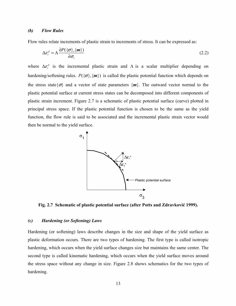
(b) Flow Rules

Flow rules relate increments of plastic strain to increments of stress. It can be expressed as:

({ },{ })pi

i

Pεσ

∂Δ = Λ∂

mσ (2.2)

where piεΔ is the incremental plastic strain and Λ is a scalar multiplier depending on

hardening/softening rules. ({ },{ })P mσ is called the plastic potential function which depends on

the stress state{σ} and a vector of state parameters {m}. The outward vector normal to the

plastic potential surface at current stress states can be decomposed into different components of

plastic strain increment. Figure 2.7 is a schematic of plastic potential surface (curve) plotted in

principal stress space. If the plastic potential function is chosen to be the same as the yield

function, the flow rule is said to be associated and the incremental plastic strain vector would

then be normal to the yield surface.

σ1

σ3

Δε1p

Δε3p

Plastic potential surface

Fig. 2.7 Schematic of plastic potential surface (after Potts and Zdravković 1999).

(c) Hardening (or Softening) Laws

Hardening (or softening) laws describe changes in the size and shape of the yield surface as

plastic deformation occurs. There are two types of hardening. The first type is called isotropic

hardening, which occurs when the yield surface changes size but maintains the same center. The

second type is called kinematic hardening, which occurs when the yield surface moves around

the stress space without any change in size. Figure 2.8 shows schematics for the two types of

hardening.

14

σ1 σ1

σ3 σ3

Isotropic hardening Kinematic hardening Fig. 2.8 Schematic of two hardening types (after Potts and Zdravković 1999).

Examples of ground response programs utilizing advanced constitutive models are

DYNAID (Prevost 1989), SUMDES (Li et al. 1992), SPECTRA (Borja and Wu 1994), AMPLE

(Pestana and Nadim 2000), and the ground response module in the OpenSees simulation

platform (Ragheb 1994; Parra 1996; Yang 2000; McKenna and Fenves 2001;

opensees.berkeley.edu).

2.2.3 Viscous Damping Formulations

Viscous damping is incorporated into most nonlinear response analysis procedures because

damping at very small strains (less than 10-4–10-2%) is not adequately captured by nonlinear

models. This occurs because the backbone curve is nearly linear at these strains, which produces

nearly zero hysteretic damping when the backbone curve is used in conjunction with the

(extended) Masing rules. The addition of a viscous damping term in the analysis avoids

unrealistic responses for problems involving small strains (Vucetic and Dobry 1986). Viscous

damping is often assumed to be proportional to both the mass and stiffness of the system. This

damping formulation, originally proposed by Rayleigh and Lindsay (1945), takes the viscous

damping matrix [C] as follows:

[ ] [ ] [ ]KaMaC 10 += (2.3)

where a0 and a1 are called Rayleigh damping coefficients.

15

Past practice has been that the viscous damping matrix is simplified by assuming that it is

proportional only to the stiffness of the soil layers, which is referred as the “simplified Rayleigh

damping formulation.” In that formulation, the calculation of the damping matrix reduces to:

[ ] [ ]KaC 1= (2.4)

and the value of viscous damping ratio, ζ, becomes

1

1

Ta πζ = (2.5)

where T1 is the period of oscillation of a target mode (usually the first mode).

If no simplification of viscous damping matrix is used, a0 and a1 take the following form:

01 2

4( )

aT T

πζ=+

(2.6)

1 21

1 2( )TTaT T

ζπ

=+

(2.7)

where T2 is the period of oscillation of another target mode. It should be noted that Equations 2.6

and 2.7 are based on the assumption that the damping ratio for the two target modes of

oscillation is the same. This “full Rayleigh damping formulation” is available in most nonlinear

ground response analysis codes.

2.3 EXAMPLES OF SPECIFIC NONLINEAR CODES

The following subsections present detailed discussions of five nonlinear codes: D-MOD_2

(Matasovic 2006) and DEEPSOIL (Hashash and Park 2001, 2002; Park and Hashash 2004;

www.uiuc.edu/~deepsoil), a ground response module in the OpenSees simulation platform

(Ragheb 1994; Parra 1996; Yang 2000; McKenna and Fenves 2001; opensees.berkeley.edu), and

SUMDES (Li et al. 1992) and TESS (Pyke 2000). All of them analyze 1D shaking, although

OpenSees and SUMDES are capable of simulating multi-dimensional shaking. The purpose of

this discussion is to illustrate the key components of nonlinear codes, and to show the types of

model parameters that are needed to use the codes. These five codes are used in subsequent

analyses presented in Chapters 4–7. Several of the codes have been revised during the course of

this project, and these revisions are presented in the respective sections below. It should be noted

that only the total stress analysis option is utilized in Chapters 4–7.

16

2.3.1 D-MOD_2

D-MOD_2 (Matasovic 2006) is an enhanced version of D-MOD (Matasovic and Vucetic 1993a).

It solves the wave propagation problem by assuming that shear waves vertically propagate

through horizontally layered soil deposits. The unbounded medium is idealized as a discrete

lumped-mass system as illustrated in Figure 2.3a. The stiffness and hysteretic damping of soil are

represented with nonlinear hysteretic springs. Additional viscous damping is included through

the use of viscous dashpots. D-MOD_2 uses the full Rayleigh viscous damping formulation

discussed in Section 2.2. An energy-transmitting boundary follows the model by Joyner and

Chen (1975) although a rigid boundary option is also available. The dynamic response scheme

used by Lee and Finn (1978) is also employed in D-MOD_2 to solve the dynamic equation of

motion in the time domain. In 2003, the Newmark β integration scheme (Newmark 1959)

replaced the Wilson θ method (Wilson 1968) to achieve a more stable numerical solution. In

addition, D-MOD_2 has a variable width shear slice option that enables a more accurate site

response calculation of levees and dams founded on bedrock. This option allows a more realistic

mass distribution (i.e., mass is made proportional to the width of the model as the width

increases with depth) and stiffness (i.e., section modulus in the horizontal plane is calculated

based upon the actual width of the slice but not based upon unit width as in conventional 1D

analysis). Moreover, D-MOD_2 is enhanced from DMOD to simulate the seismically induced

slip that may occur along the weak interfaces.

(a) Backbone Curve

D-MOD_2 incorporates the MKZ constitutive model (Matasovic and Vucetic 1993a) to define

the initial backbone curve. The MKZ constitutive model is presented in Figure 2.9. The MKZ

model is a modification of the hyperbolic model by Kondner and Zelasko (1963) (KZ model).

Two curve-fitting constants α and s are added to the KZ model, and the normalized form of the

MKZ model is given by:

s

mo

mo

mo

G

G

⎟⎟⎠

⎞⎜⎜⎝

⎛+

=

γτ

α

γτ

*

*

**

1

(2.8)

17

where vcmomo GG '/* σ= , vcmomo '/* σττ = , σ’vc = initial vertical effective stress, Gmo = initial

shear modulus, and τmo = shear strength of the soil.

Fig. 2.9 Schematic illustration of MKZ constitutive model showing stress-strain behavior in first cycle (at time t=0) and subsequent cycle (at time t).

The original KZ model was intended to cover a large range of strains all the way up to

failure. However, the dominant strains in the seismic response of soil deposits are relatively

small, usually less than 1–3%, which are much lower than typical static failure strains in soil. In

order to model accurately the initial loading curve, Matasovic and Vucetic (1993a) suggested

that τmo can be arbitrarily chosen as the τ ordinate corresponding approximately to the upper

boundary of the dominant shear strain range. Figure 2.10 shows how different values of mo*τ

affect the KZ model prediction on the positive portion of the initial backbone curve. Note that

the prediction by the MKZ model shown in Figure 2.10 used mo*τ corresponding to a shear strain

of 1%.

18

Fig. 2.10 Comparison of positive portion of initial backbone curves obtained from KZ and MKZ models (Matasovic and Vucetic 1993a).

The ratio * */mo moGτ is often termed the reference shear strain (Hardin and Drnevich

1972) and is considered to be a material constant (see Section 4.1). Parameters α and s were

introduced in the MKZ model and, as shown in Figure 2.10, the approximation of the initial

backbone curve from experimental data is improved when MKZ model is used in lieu of the KZ

model. Matasovic and Vucetic (1993a) found that the range of α for sand is ≈ 1.0–1.9, while the

range of s is ≈ 0.67–0.98. As shown in Figure 2.11, the modulus reduction curves obtained from

the MKZ models were found to be in agreement with experimental data.

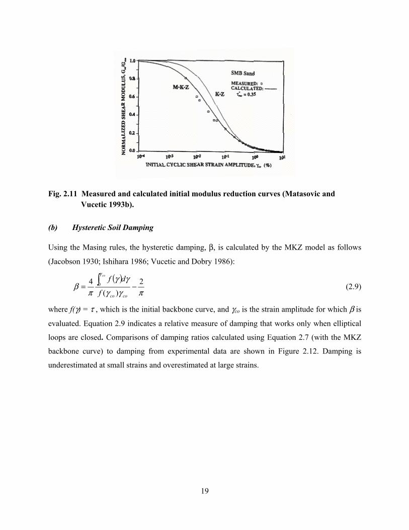
19

Fig. 2.11 Measured and calculated initial modulus reduction curves (Matasovic and Vucetic 1993b).

(b) Hysteretic Soil Damping

Using the Masing rules, the hysteretic damping, β, is calculated by the MKZ model as follows

(Jacobson 1930; Ishihara 1986; Vucetic and Dobry 1986):

( )πγγ

γγ

πβ

γ

2)(

4 0 −= ∫cocof

dfco

(2.9)

where f(γ) = τ , which is the initial backbone curve, and γco is the strain amplitude for which β is

evaluated. Equation 2.9 indicates a relative measure of damping that works only when elliptical

loops are closed. Comparisons of damping ratios calculated using Equation 2.7 (with the MKZ

backbone curve) to damping from experimental data are shown in Figure 2.12. Damping is

underestimated at small strains and overestimated at large strains.

20

Fig. 2.12 Measured and calculated initial damping curves (Matasovic and Vucetic 1993a).

(c) Material Degradation

The degradation of material strength and stiffness with repeated cycling is taken into account

with the use of degradation index functions for modulus (δG) and strength (δτ). Degradation

functions used for sand and clay are shown in Table 2.2. Incorporating these degradation

functions into the equation for the MKZ backbone curve (originally given in Eq. 2.6) leads to the

following equation:

s

mo

moG

moG

G

G

⎟⎟⎠

⎞⎜⎜⎝

⎛+

=

γτδ

δα

γδτ

τ*

*

**

1

(2.10)

21

Table 2.2 Degradation index functions and corresponding coefficients (Matasovic and Vucetic 1993b).

Coefficients Material Degradation Index Function

ν t

δG = [1 - u*]0.5 - - Sand

δτ = [1- (u*)ν] 1.0-5.0 -

Clay δG = δτ = δ = N-t - t = f(PI, OCR, γc, γtup)

As shown in Table 2.2, different forms of degradation index functions are used for sand

and clay. For sand, cyclic degradation is mainly a function of the normalized residual cyclic pore

pressure, u* ≡ u / σ’vc. Parameter ν is a fitting parameter for strength degradation and increases as

the degradation becomes more pronounced. Figure 2.13 shows degraded backbone curves

obtained with different values of u*. The pore-water pressure model for saturated sand layers

implemented in D-MOD_2 was originally developed by Dobry et al. (1985) and modified by

Vucetic and Dobry (1986). This model allows the evaluation of the normalized residual cyclic

pore pressure after cycle Nc as follows:

btupctc

btupctc

N FNfFNfp

u).(..1).(...*

γγγγ

−+−

= (2.11)

where γct is the cyclic shear strain amplitude and γtup is the volumetric threshold shear strain

below which no significant pore-water pressure is generated, and is usually between 0.01 and

0.02% for most sands (Dobry et al. 1982; Vucetic 1994). Parameter f can be taken as 1 or 2,

depending on whether pore pressures are generated by shaking in one or two directions.

Parameters F, p, and b are obtained by fitting laboratory data from cyclic strain-controlled tests.

The above formulation is for symmetrical cyclic loading and can be modified to account for

irregular cyclic loading. This procedure was originally introduced by Finn et al. (1977) and

modified by Vucetic and Dobry (1986). A detailed description of the procedure can be found in

Vucetic and Dobry (1986).

22

Fig. 2.13 Families of degraded backbone curves (Matasovic and Vucetic 1993a).

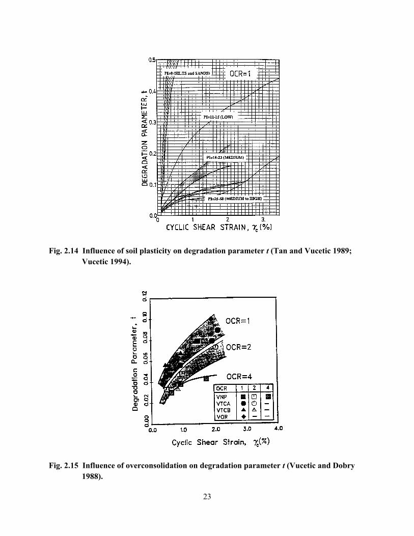
For clay, cyclic degradation can result from both pore-water pressure generation and

deterioration of clay microstructure. As indicated in Table 2.2, the degradation function for clay

takes the form of N-t (Idriss et al. 1978) where t = g(γct -γtup)r. Parameters g and r are curve-

fitting parameters introduced by Pyke (2000). In general, t is a function of the overconsolidation

ratio (OCR) and plasticity index (PI) as shown in Figures 2.14–2.15. In D-MOD_2, residual

pore-water pressure after cycle N is expressed as (Matasovic and Vucetic 1995):

DCNBNANu ttN +++= −−− 23* (2.12)

where A, B, C, and D are fitting constants that are determined experimentally.

23

Fig. 2.14 Influence of soil plasticity on degradation parameter t (Tan and Vucetic 1989; Vucetic 1994).

Fig. 2.15 Influence of overconsolidation on degradation parameter t (Vucetic and Dobry

1988).

24

D-MOD_2 includes a pore-water pressure dissipation and redistribution model, which

was originally used in DESRA-2 (Lee and Finn 1978). This is to account for the fact that if a

saturated layer can drain, simultaneous generation, dissipation, and redistribution of pore-water

pressure during and after shaking are possible. This may in turn have a significant impact on the

magnitudes of residual pore-water pressures. The model employed in D-MOD_2 was taken from

Lee and Finn (1975, 1978) and Martin and Seed (1978) and can be written as: 2

2r

cyw st

u k u uEt z tγ

⎛ ⎞∂ ∂ ∂⎛ ⎞= +⎜ ⎟ ⎜ ⎟∂ ∂ ∂⎝ ⎠⎝ ⎠ (2.13)

where u, rE , k, and γw represent pore pressure, constrained rebound modulus, hydraulic

conductivity, and unit weight of water, respectively. The first term of the right-hand side of

Equation 2.13. represents the effects of dissipation via Terzaghi’s 1D consolidation equation,

while the second term represents the rate of cyclic pore-water pressure development. This

differential equation is solved using a slightly modified finite difference solution from DESRA-

2.

(d) Viscous Damping

Full Rayleigh damping formulation is used in D-MOD_2.

(e) Summary of Input Parameters

The following seven types of input parameters are needed to implement D-MOD_2 for dynamic

nonlinear response analysis:

1. Parameters to define the MKZ backbone curve: initial tangent shear modulus of soil, Gmo,

shear stress at reference strain, τmo, and curve-fitting constants, α and s;

2. Parameters for cyclic degradation: ν (for sand), g and r (for clay), and volumetric

threshold shear strain, γtup;

3. Parameters for pore-water pressure generation model of sand: f (either 1 or 2), curve-

fitting constants p, F, and b;

4. Parameters for pore-water pressure generation model of clay: fitting constants A, B, C, D;

25

5. Parameters for the pore-water pressure dissipation and redistribution model: constrained

rebound modulus, rE or hydraulic conductivity, k, and other constants to define the

Martin et al. (1975) model;

6. Properties of each layer and visco-elastic halfspace: width, thickness, saturated unit

weight, and wet unit weight for each layer, unit weight and shear wave velocity of visco-

elastic halfspace;

7. Rayleigh damping coefficients.

Parameters (1)–(6) correspond to parameters that are related to soil profile conditions and soil

properties. Some of these parameters can be readily evaluated from the data generated in a

typical geotechnical investigation, while others cannot. In addition to soil properties, the

parameters in (7) require a relatively high degree of judgment and are not uniquely related to

ordinary soil properties. For total stress analyses, only the parameters in (1) and (7) are needed.

2.3.2 DEEPSOIL

The DEEPSOIL code includes equivalent-linear and nonlinear analysis modes. The equivalent-

linear analysis mode is similar to other available codes (e.g., SHAKE). It has no limitations on

the number of layers, material properties, or length of input motion. The implementation includes

a robust convergence algorithm and several choices for complex shear modulus formulation. The

nonlinear mode is described next.

(a) Backbone Curve

DEEPSOIL (Hashash and Park 2001, 2002; Park and Hashash 2004) is a nonlinear site response

analysis model for vertical propagation of horizontal shear waves in deep soil deposits. The code

utilizes the same MDOF lumped-mass system as DESRA-2. The dynamical equilibrium equation

of motion is solved numerically using the Newmark β method (1959). The DEEPSOIL version

used in this document (V2.6) uses a total stress analysis approach. At the writing of this

document, an effective stress analysis component has been implemented in the computational

engine of DEEPSOIL and is being integrated with the user interface. The nonlinear constitutive

model used in DEEPSOIL is based on the MKZ model, but Hashash and Park (2001) modified

the reference strain definition as follows:

26

b

ref

vor a ⎟

⎟⎠

⎞⎜⎜⎝

⎛=

σσγ '

(2.14)

where 'voσ and refσ represent effective vertical stress and reference confining pressure,

respectively, and parameters a and b are curve-fitting parameters for the initial backbone curve

and can be determined from experimental data for a particular type of soil. This modification is

to allow the reference strain to be pressure dependent.

The hysteretic model utilized in DEEPSOIL is given by:

s

r

moG

⎟⎟⎠

⎞⎜⎜⎝

⎛+

=

γγα

γτ

1

(2.15)

Figure 2.16 (top frame) shows the match of the modified MKZ model to experimental modulus

reduction curves by Laird and Stokoe (1993).

27

Fig. 2.16 Comparisons of modulus reduction curves (top frame) and damping curves

(bottom frame) obtained from Hashash and Park (2001) modified MKZ model with Laird and Stokoe (1993) experimental data.

(b) Hysteretic Soil Damping

Hysteretic soil damping in DEEPSOIL is evaluated using the backbone curve in conjunction

with the Masing criteria. The procedure is essentially the same as that presented in Section

2.3.1b.

Experimental data show a dependence of soil damping at very small strains on confining

pressure. Hashash and Park (2001) therefore proposed the small-strain hysteretic damping ratio,

denoted “zero strain equivalent” damping ratio ζs. Parameter ζs is taken as follows:

( )dsc'σ

ζ = (2.16)

where c and d are fitting constants determined experimentally. Figure 2.16 (bottom frame) shows

that the proposed pressure-dependent damping ratio equation matches the experimental data well

at small strains.

28

(c) Viscous Damping Term

DEEPSOIL allows viscous damping to be specified using simplified or full Rayleigh damping

schemes as described in Section 2.2.3. In addition, DEEPSOIL incorporates an extended

Rayleigh viscous damping formulation. In this formulation, the damping matrix can consist of

any combination of mass and stiffness matrices (Clough and Penzien 1993) and is given by:

[ ] [ ] [ ] [ ][ ] e

e

bN

bb KMaMC ∑

−−=

11 (2.17)

where N is the number of modes incorporated. The damping ratio ζn can be expressed as:

bn

N

bb

nn fa

f2

1

0)2(

41 ∑

−

=

= ππ

ζ (2.18)

Park and Hashash (2004) included four modes in their study and thus ab is found by:

⎪⎪⎭

⎪⎪⎬

⎫

⎪⎪⎩

⎪⎪⎨

⎧

⎥⎥⎥⎥⎥⎥⎥⎥⎥

⎦

⎤

⎢⎢⎢⎢⎢⎢⎢⎢⎢

⎣

⎡

=

⎥⎥⎥⎥⎥

⎦

⎤

⎢⎢⎢⎢⎢

⎣

⎡

3

2

1

0

52

2

52

52

1

1

1

1

41

aaaa

ffff

ffff

ffff

ffff

pppp

oooo

nnnn

mmmm

p

o

n

m

πζζζζ

(2.19)

where fm, fn , fo, and fp are selected frequencies and ζm, ζn, ζo, and ζp are the damping ratios at

these frequencies that may take the value of the zero strain equivalent damping ratio in Equation

(2.16). Park and Hashash (2004) performed linear wave propagation analysis, and found that

time-domain solutions using the extended Rayleigh damping formulation are closer to the

frequency-domain solution than time-domain solutions developed using simplified or full

Rayleigh damping. Park and Hashash suggested that the first two frequencies can be chosen in

part to cover the range of frequencies where there is significant energy in the input motion. The

third and fourth frequencies should be approximately 10 Hz. In general, they recommended that

an iterative procedure should be performed and the selected frequencies should give the best

agreement between the results of a linear time-domain analysis and a linear frequency-domain

solution.

29

(d) Summary of Input Parameters

For DEEPSOIL, four types of soil profile properties are needed:

1. Parameters to define the modified MKZ backbone curve: initial tangent shear modulus of

soil, Gmo, shear stress at reference strain, τmo, and curve-fitting constants, α, s; a and b;


weight, and wet unit weight for each layer, and unit weight and shear wave velocity of

visco-elastic halfspace;

3. Viscous damping ratios and frequencies for the Rayleigh damping formulation.

The parameters in (1)–(2) correspond to parameters that are related to soil profile conditions and

soil properties. In addition to soil properties, the parameters in (3) require a relatively high

degree of judgment and are not uniquely related to ordinary soil properties.

2.3.3 TESS

(a) Backbone Curve

TESS is a 1D site response analysis code that utilizes the explicit finite difference scheme to

solve the equation of motion. The backbone curve used in TESS is a hyperbolic function similar

to that used in D-MOD_2 and DEEPSOIL. The form of the equation used in TESS is:

1

moa

mo

mo

G

G

γτγ

τ

=⎛ ⎞

+ ⎜ ⎟⎝ ⎠

(2.20)

where Gmo is the initial small-strain shear modulus, ratio τmo/Gmo is the reference strain, and a is

a fitting parameter.

(b) Hysteretic Damping

Hysteretic soil damping in TESS is evaluated using the backbone curve in conjunction with the

Cundall-Pyke hypothesis (Pyke 1979). This hypothesis represents a modification of Masing rules

and is discussed in detail in Section 5.4. Similar to the Masing rules, the Cundall-Pyke

hypothesis underestimates damping at small strains and overestimates damping at large strains.

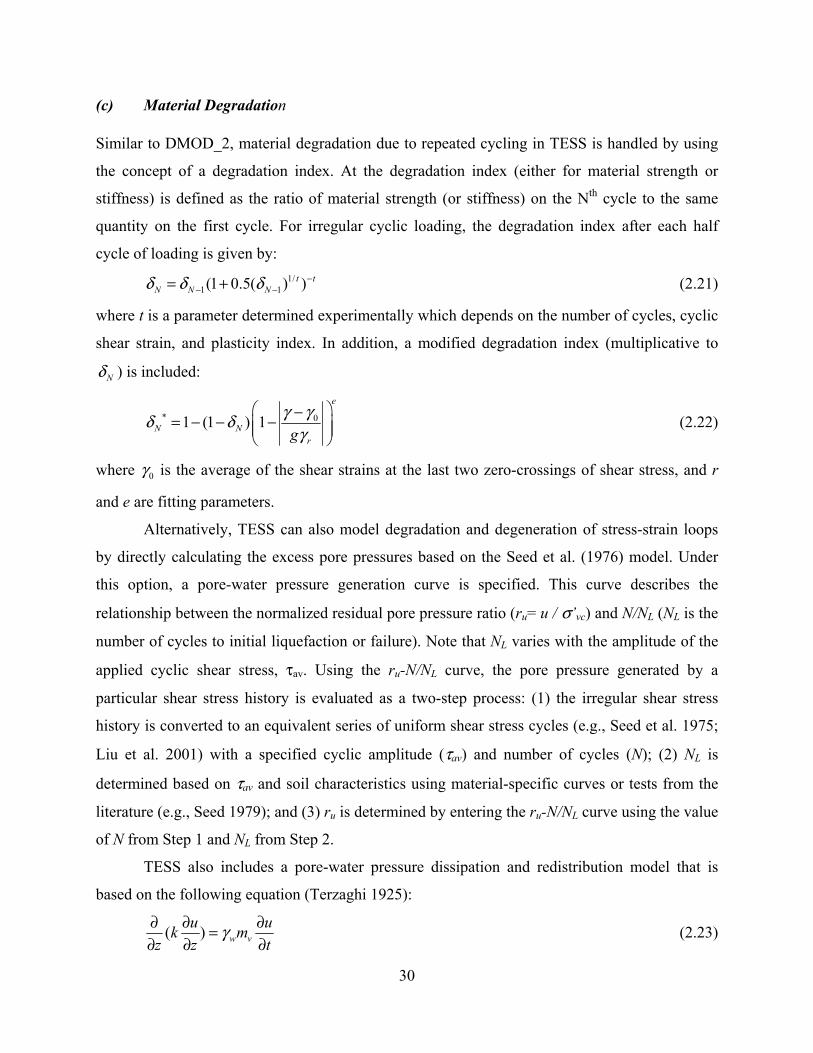
30

(c) Material Degradation

Similar to DMOD_2, material degradation due to repeated cycling in TESS is handled by using

the concept of a degradation index. At the degradation index (either for material strength or

stiffness) is defined as the ratio of material strength (or stiffness) on the Nth cycle to the same

quantity on the first cycle. For irregular cyclic loading, the degradation index after each half

cycle of loading is given by: 1/

1 1(1 0.5( ) )t tN N Nδ δ δ −

− −= + (2.21)

where t is a parameter determined experimentally which depends on the number of cycles, cyclic

shear strain, and plasticity index. In addition, a modified degradation index (multiplicative to

Nδ ) is included:

* 01 (1 ) 1e

N Nrg

γ γδ δγ

⎛ ⎞−= − − −⎜ ⎟⎜ ⎟⎝ ⎠

(2.22)

where 0γ is the average of the shear strains at the last two zero-crossings of shear stress, and r

and e are fitting parameters.

Alternatively, TESS can also model degradation and degeneration of stress-strain loops

by directly calculating the excess pore pressures based on the Seed et al. (1976) model. Under

this option, a pore-water pressure generation curve is specified. This curve describes the

relationship between the normalized residual pore pressure ratio (ru= u / σ’vc) and N/NL (NL is the

number of cycles to initial liquefaction or failure). Note that NL varies with the amplitude of the

applied cyclic shear stress, τav. Using the ru-N/NL curve, the pore pressure generated by a

particular shear stress history is evaluated as a two-step process: (1) the irregular shear stress

history is converted to an equivalent series of uniform shear stress cycles (e.g., Seed et al. 1975;

Liu et al. 2001) with a specified cyclic amplitude (τav) and number of cycles (N); (2) NL is

determined based on τav and soil characteristics using material-specific curves or tests from the

literature (e.g., Seed 1979); and (3) ru is determined by entering the ru-N/NL curve using the value

of N from Step 1 and NL from Step 2.

TESS also includes a pore-water pressure dissipation and redistribution model that is

based on the following equation (Terzaghi 1925):

( ) w vu uk m

z z tγ∂ ∂ ∂=

∂ ∂ ∂ (2.23)

31

where k, γw, and mv are the permeability of soil, coefficient of volume, change of soil, and unit

weight of water, respectively.

(d) Low-Strain Damping Scheme

Unlike the other nonlinear codes presented in this section, TESS does not have a viscous

damping scheme. Instead, it has a low-strain (hysteretic) damping scheme that produces non-zero

hysteretic damping at small strains. The most recent version of this scheme is discussed in detail

in Section 5.4.

(e) Summary of Parameters

For TESS, three types of soil profile properties are needed:

1. Parameters describing the initial backbone curve: initial tangent shear modulus of soil,

Gmo, shear stress at reference strain, τmo, and curve-fitting constants, a

2. Parameters controlling the degradation of shear modulus and shear strength (either

through the degradation parameters or specification of pore pressure generation curve and

NL)

3. Parameters controlling pore pressure generation and dissipation


weight and wet unit weight for each layer, and unit weight and shear wave velocity of

visco-elastic halfspace;

5. Parameters controlling the low strain damping scheme

2.3.4 OpenSees

The ground response module in the OpenSees simulation platform (Ragheb 1994; Parra 1996;

Yang 2000; McKenna and Fenves 2001; opensees.berkeley.edu) utilized a two-phase (solid-

fluid) fully coupled finite element (FE) formulation which is capable of simulating permanent

shear-strain accumulation in clean medium-dense cohesionless soils during liquefaction and

dilation due to increased cyclic shear stiffness and strength. The constitutive model is based on

the framework of multi-surface (nested-surface) plasticity (Iwan 1967; Prevost 1985; Mroz

1967), with modifications by Yang (2000). The major components of the plasticity model (in

32

terms of yield function, hardening rule, and flow rule) are briefly described below (more detailed

descriptions can be found from Kramer and Elgamal. 2001; Parra 1996; Yang 2000), which is

then followed by a summary of input parameters needed for analysis.

(a) Yield Function

For clay, which undergoes fast undrained loading during earthquakes, the yield function is

assumed to follow the Von Mises shape, which is illustrated in Figure 2.17. The Von Mises yield

surface is a function solely of undrained shear strength. For sand, which may exhibit within-

cycle pore pressure induced softening followed by relatively large strain dilatancy during

earthquake shaking, the yield function is assumed to follow the Drucker-Prager shape, as

illustrated in Figure 2.18. The Drucker-Prager yield surface is described in effective stress space

as a function of friction angle and cohesion (as defined in the Mohr-Coulomb failure criteria).

Both yield surface types are incorporated into the multi-surface framework.

(b) Hardening Rule

A purely deviatoric kinematic hardening rule (Prevost 1985) is employed in order to generate

soil hysteretic response under cyclic loading. This kinematic rule dictates that all yield surfaces

may translate in stress space within the failure envelope (Parra 1996; Yang 2000) and is

consistent with the Masing unloading/reloading criteria.

Under drained monotonic shear loading, the hardening zone is represented by a number

of similar yield surfaces for which the (tangent) elastoplastic modulus can be defined by using a

piecewise linear approximation of a hyperbolic backbone curve. As shown in Figure 2.19, each

linear segment represents the domain of a yield surface fm with a shear modulus Hm and size Mm,

for m = 1, 2, ..., NYS (= total number of yield surfaces). Hm is defined by

mm

mmmH

γγττ

−−

=+

+

1

1 )(2 (2.24)

where HNYS = 0. It should be noted that the outermost surface is the envelope of peak shear

strength (failure size), the size of which can be calculated as:

6sin3 sinf NYSM M φ

φ= =

− (2.25)

where φ is the friction angle.

33

σ2

σ3

σ1

σ1σ3

σ2

Fig. 2.17 Cylindrical Von Mises yield surfaces for clay (after Prevost 1985, Lacy 1986,

Parra 1996, and Yang 2000).

σ2'

σ3'

σ1'

σ1'σ3'

σ2'

Fig. 2.18 Conical Drucker-Prager yield surfaces for sand (after Prevost 1985, Lacy 1986,

Parra 1996, and Yang 2000).

Fig. 2.19 Hyperbolic backbone curve for soil nonlinear shear stress-strain response and

piecewise-linear representation in multi-surface plasticity (after Prevost 1985 and Parra 1996).

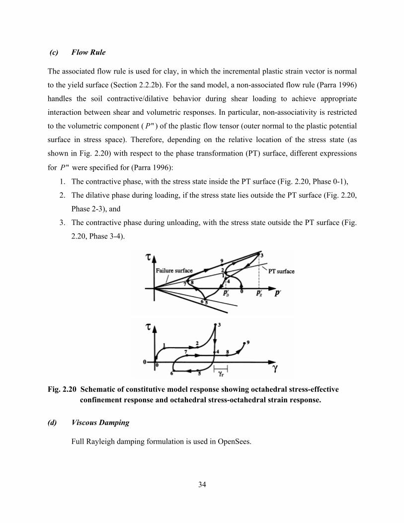
34

(c) Flow Rule

The associated flow rule is used for clay, in which the incremental plastic strain vector is normal

to the yield surface (Section 2.2.2b). For the sand model, a non-associated flow rule (Parra 1996)

handles the soil contractive/dilative behavior during shear loading to achieve appropriate

interaction between shear and volumetric responses. In particular, non-associativity is restricted

to the volumetric component ( "P ) of the plastic flow tensor (outer normal to the plastic potential

surface in stress space). Therefore, depending on the relative location of the stress state (as

shown in Fig. 2.20) with respect to the phase transformation (PT) surface, different expressions

for "P were specified for (Parra 1996):

1. The contractive phase, with the stress state inside the PT surface (Fig. 2.20, Phase 0-1),

2. The dilative phase during loading, if the stress state lies outside the PT surface (Fig. 2.20,

Phase 2-3), and

3. The contractive phase during unloading, with the stress state outside the PT surface (Fig.

2.20, Phase 3-4).

Fig. 2.20 Schematic of constitutive model response showing octahedral stress-effective

confinement response and octahedral stress-octahedral strain response.

(d) Viscous Damping

Full Rayleigh damping formulation is used in OpenSees.

35


For OpenSees, four types of soil profile properties are needed:

1. Parameters describing the yield surfaces (for both sand and clay): either defining the

modulus reduction at different strain values or a hyperbolic backbone curve (in terms of

small-strain shear modulus and reference strain)

2. Parameters controlling contraction and dilatency response.

3. Properties of each layer and visco-elastic halfspace: thickness, saturated (or wet) unit

weight, low-strain shear modulus and bulk modulus; unit weight and shear wave velocity

of visco-elastic halfspace;

4. Frequencies/modes for the Rayleigh damping formulation.

2.3.5 SUMDES

SUMDES (Li et al. 1992) is a nonlinear finite element program which can model the dynamic

response of sites under multi-directional earthquake shaking. It utilizes an effective stress

approach, and wave propagation and diffusion effects are fully coupled. It can predict three-

directional motions as well as pore pressure build-up and dissipation within soil deposits. The

soil constitutive model is based on the bounding surface hypoplasticity model (Wang 1990;

Wang et al. 1990) in which the incremental plastic strain vector direction depends on the

incremental stress direction (in addition to the stress state). The major components of this

plasticity model (in terms of yield function, hardening rule, and flow rule) are described briefly

below, which is then followed by a summary of input parameters needed for analysis.

(a) Yield Function

The plasticity framework consists of a bounding surface (or a failure surface) which is similar to

a conventional yield surface. However, elasto-plastic behavior occurs when the stress state is

inside the bounding surface. A maximum prestress memory surface is also defined. This serves

as the first bounding surface, the shape of which is similar to the yield surface. A new loading

surface forms as loading occurs inside the maximum prestress memory surface. The relative

position of the current loading surface with respect to the maximum prestress memory surface

and bounding surface would determine the elasto-plastic behavior for the current stress state.

36

Similar to the outermost yield surface in OpenSees, the bounding (failure) surface is related to

the friction angle, as given by Equation 2.25. Figure 2.21 is a schematic of the yield surfaces, the

maximum prestress memory surface (the middle one), and the loading surface (in dash line),

used in the bounding surface hypoplasticity framework. The flow rule can be related to the

normal at the maximum prestress memory surface as well as the normal on the failure surface

(when the “rotational shear” effect is simulated as needed).

Fig 2.21 Schematic of the bounding surface plasticity framework (after Wang et al. 1990).

(b) Hardening Rule

A kinematic hardening rule is employed to simulate soil hysteretic response under cyclic loading.

This rule is consistent with the Masing unloading/reloading scheme. Similar to OpenSees, the

plastic shear modulus in the hardening zone can be determined from a modulus reduction curve

(hence the backbone curve). However, only one parameter, called hr, is used in the calibration

process.

(c) Flow Rule

Non-associated flow rule is used to handle the soil contractive/dilative behavior. Similar to

OpenSees, different flow rules are used depending on the relative location of the stress state (as

shown in Fig. 2.22) with respect to the phase transformation surface (the slope of which is

defined as Rp in SUMDES).

37

Fig. 2.22 Schematic showing stress-confinement response (after Li et. al. 1992).

(d) Viscous Damping Formulation

Only the simplified Rayleigh damping formulation is available in SUMDES. It is assumed by the

program that the damping ratio is given at 1 Hz. Any desired damping ratio at a desired

frequency (e.g., fs) can be converted to a damping ratio at 1 Hz using simple proportionality, e.g.,

ζf = ζfs /fs. This is because in the simplified Rayleigh damping formulation, the damping ratio is

proportional to the frequency.


For SUMDES, four types of soil profile properties are needed:

1. Parameter controlling the plastic shear modulus (which can be determined from the

modulus reduction curve and some basic soil profile properties including void ratio,

initial tangent shear modulus, shear strength, and mean normal stress);

2. Parameters controlling contraction and dilation response;


weight, and wet unit weight for each layer, unit weight. and shear wave velocity of visco-

elastic halfspace; and

4. Viscous damping ratio for the simplified Rayleigh damping formulation.

38

2.4 VERIFICATION STUDIES OF GROUND RESPONSE ANALYSIS CODES

The effectiveness of 1D ground response analysis schemes can be studied when a rock recording

is available near a soil recording, or when vertical array data are available. In this section, several

studies that have utilized either rock/soil recording pairs or vertical array data to investigate the

ability of 1D ground response analyses to simulate observed site effects are discussed.

Verification studies utilizing rock/soil recording pairs take the rock motion as input to

ground response analysis, and the computed and recorded soil motions are compared. Several

examples of studies of this type are summarized in Table 2.3. For example, Dickenson (1994)

used SHAKE and MARDESRA to study the ground response of 11 Bay Mud soft soil sites in the

San Francisco Bay Area and found that both models were able to predict reasonably well

variations between soil/rock spectra across a broad period range (Fig. 2.23). Chang (1996) and

Chang et al. (1996) used SHAKE and DMOD to study ground response effects for deep clay

sites in both northern California and Los Angeles area alluvial sites. They found that predictions

were relatively good for the northern California sites for T < 1s (e.g., Fig. 2.24a) and relatively

poor for the Los Angeles sites (e.g., Fig. 2.24b). They concluded that the difference in model

accuracy at Bay Area and Los Angeles area sites may be associated with basin effects

(particularly at long periods) because the geometry at the Bay Area sites is relatively wide and

flat as compared to the Los Angeles area sedimentary basins. It should be noted that no formal

parameter selection protocols were followed when conducting the nonlinear ground response

analyses for these sites—hence, some adjustments of key parameters to match observed

responses were possible.

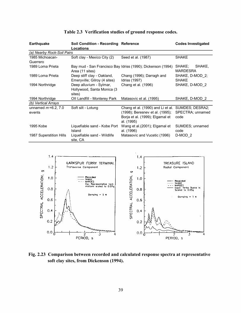
39

Table 2.3 Verification studies of ground response codes.

Earthquake Soil Condition - Recording Locations

Reference Codes Investigated

(a) Nearby Rock-Soil Pairs1985 Michoacan-Guerrero

Soft clay - Mexico City (2) Seed et al. (1987) SHAKE

1989 Loma Prieta Bay mud - San Francisco Bay Area (11 sites)

Idriss (1990); Dickenson (1994) SHAKE; SHAKE, MARDESRA

1989 Loma Prieta Deep stiff clay - Oakland, Emeryville; Gilroy (4 sites)

Chang (1996); Darragh and Idriss (1997)

SHAKE, D-MOD_2; SHAKE

1994 Northridge Deep alluvium - Sylmar, Hollywood, Santa Monica (3 sites)

Chang et al. (1996) SHAKE, D-MOD_2

1994 Northridge OII Landfill - Monterey Park Matasovic et al. (1995) SHAKE, D-MOD_2(b) Vertical Arraysunnamed m =6.2, 7.0 events

Soft silt - Lotung Chang et al. (1990) and Li et al. (1998); Beresnev et al. (1995); Borja et al. (1999); Elgamal et al. (1995)

SUMDES; DESRA2; SPECTRA; unnamed code

1995 Kobe Liquefiable sand - Kobe Port Island

Wang et al.(2001); Elgamal et al. (1996)

SUMDES; unnamed code

1987 Superstition Hills Liquefiable sand - Wildlife site, CA

Matasovic and Vucetic (1996) D-MOD_2

Fig. 2.23 Comparison between recorded and calculated response spectra at representative soft clay sites, from Dickenson (1994).

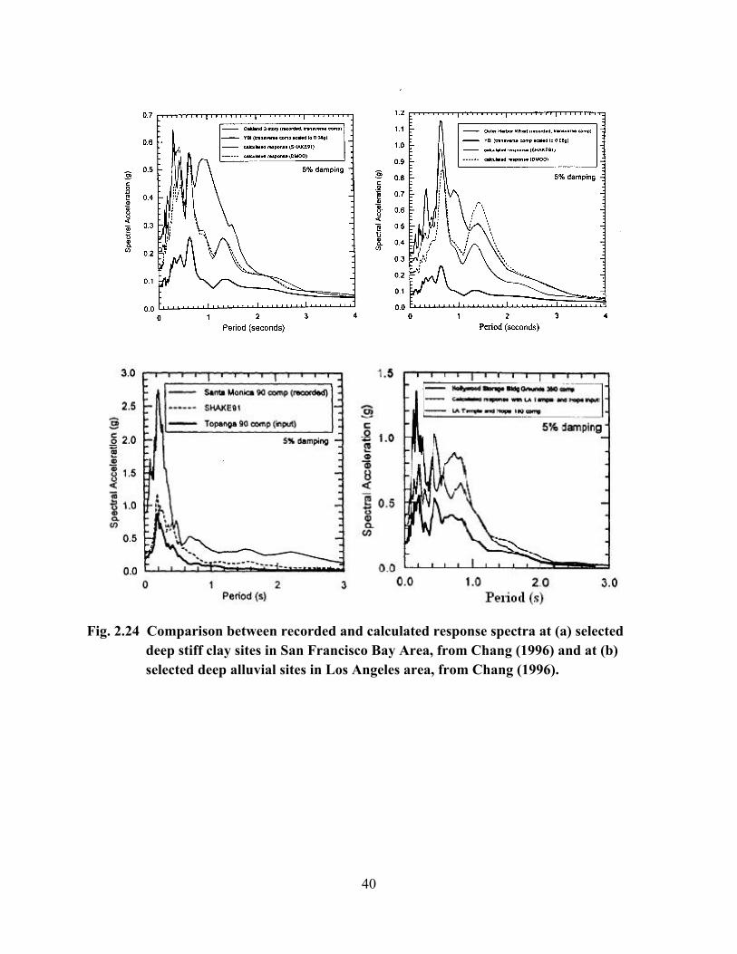
40

Fig. 2.24 Comparison between recorded and calculated response spectra at (a) selected

deep stiff clay sites in San Francisco Bay Area, from Chang (1996) and at (b) selected deep alluvial sites in Los Angeles area, from Chang (1996).

41

One important outcome of the above studies is that the accuracy of predicted spectra on

soil depends significantly on the rock (control) motion characteristics. This was well illustrated

by Idriss (1993), who found that predicted spectra at the Treasure Island soil site is matched well

when the control rock motion is taken from nearby Yerba Buena Island (Fig. 2.25, top frame),

but is matched relatively poorly when control motions are taken from other San-Francisco-

Oakland–Berkeley area rock stations (Fig. 2.25, bottom frame). Since in a design setting the

detailed characteristics of rock motions cannot be known precisely, it is clear that significant

uncertainty is introduced to predicted soil spectra from uncertainly in input motion

characteristics.

A more direct verification of 1D ground response analyses can be performed using

recordings from vertical arrays. Examples of a few prior studies that have utilized vertical array

data to validate ground response analysis codes are listed in Table 2.3. Lotung, a non-liquefiable

large-scale seismic test site in Taiwan, is one of the vertical arrays that is used to validate various

ground response analysis codes. Figure 2.26 shows the results of such analyses obtained from

both a nonlinear analysis code (SPECTRA) as well as SHAKE. Borja et al. (1999) found that

both analysis procedures provided good predictions in the time domain to the recorded motions.

42

Fig. 2.25 Comparison of acceleration response spectrum of recorded motion at Treasure Island strong motion site (1989 Loma Prieta earthquake) with calculated spectra from ground response analyses. Calculations in upper frame utilized nearby rock recording (Yerba Buena Island) as control motion; lower frame presents statistical variation in calculated spectra for suite of control motions from rock sites in region surrounding Treasure Island. From Idriss 1993.

43

Fig. 2.26 Comparison of recorded ground surface accelerations and predictions by

SHAKE (top two frames) and SPECTRA (third frame from top). Bottom frame shows recording at base of array (47-m depth). After Borja et al. 1999.

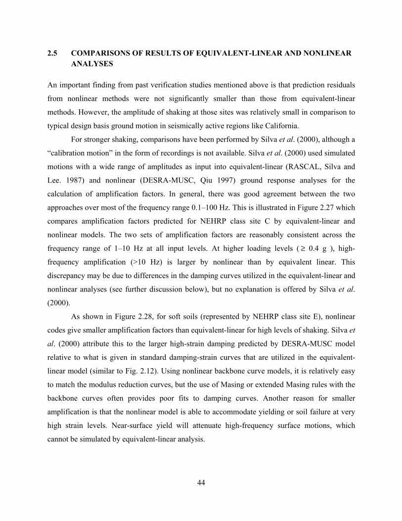
44

2.5 COMPARISONS OF RESULTS OF EQUIVALENT-LINEAR AND NONLINEAR ANALYSES

An important finding from past verification studies mentioned above is that prediction residuals

from nonlinear methods were not significantly smaller than those from equivalent-linear

methods. However, the amplitude of shaking at those sites was relatively small in comparison to

typical design basis ground motion in seismically active regions like California.

For stronger shaking, comparisons have been performed by Silva et al. (2000), although a

“calibration motion” in the form of recordings is not available. Silva et al. (2000) used simulated

motions with a wide range of amplitudes as input into equivalent-linear (RASCAL, Silva and

Lee. 1987) and nonlinear (DESRA-MUSC, Qiu 1997) ground response analyses for the

calculation of amplification factors. In general, there was good agreement between the two

approaches over most of the frequency range 0.1–100 Hz. This is illustrated in Figure 2.27 which

compares amplification factors predicted for NEHRP class site C by equivalent-linear and

nonlinear models. The two sets of amplification factors are reasonably consistent across the

frequency range of 1–10 Hz at all input levels. At higher loading levels ( ≥ 0.4 g ), high-

frequency amplification (>10 Hz) is larger by nonlinear than by equivalent linear. This

discrepancy may be due to differences in the damping curves utilized in the equivalent-linear and

nonlinear analyses (see further discussion below), but no explanation is offered by Silva et al.

(2000).

As shown in Figure 2.28, for soft soils (represented by NEHRP class site E), nonlinear

codes give smaller amplification factors than equivalent-linear for high levels of shaking. Silva et

al. (2000) attribute this to the larger high-strain damping predicted by DESRA-MUSC model

relative to what is given in standard damping-strain curves that are utilized in the equivalent-

linear model (similar to Fig. 2.12). Using nonlinear backbone curve models, it is relatively easy

to match the modulus reduction curves, but the use of Masing or extended Masing rules with the

backbone curves often provides poor fits to damping curves. Another reason for smaller

amplification is that the nonlinear model is able to accommodate yielding or soil failure at very

high strain levels. Near-surface yield will attenuate high-frequency surface motions, which

cannot be simulated by equivalent-linear analysis.

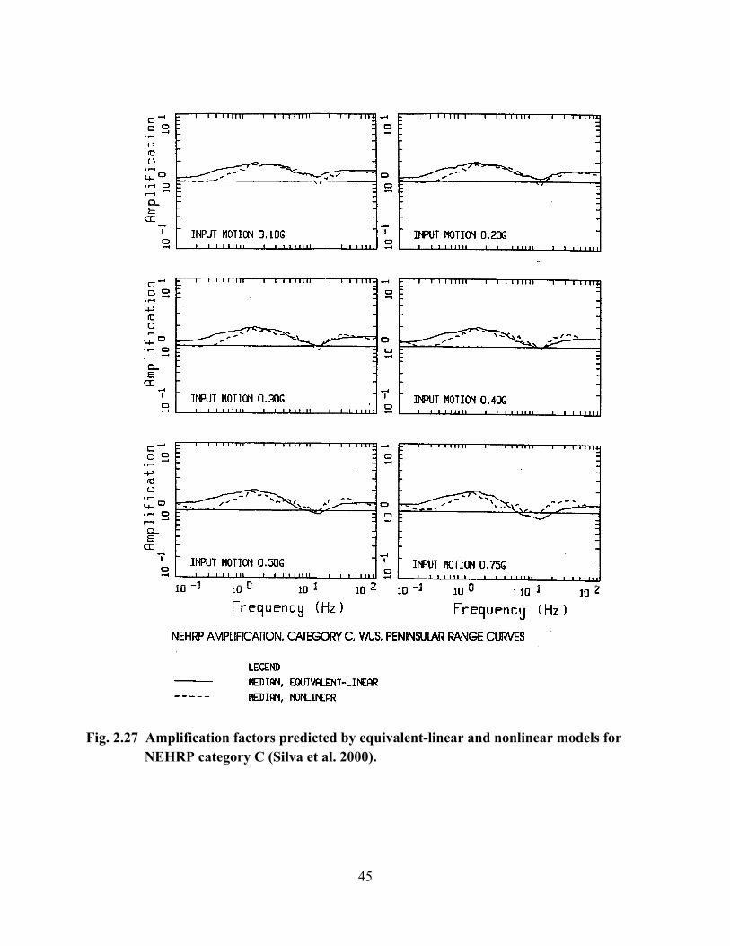
45

Fig. 2.27 Amplification factors predicted by equivalent-linear and nonlinear models for NEHRP category C (Silva et al. 2000).

46

Fig. 2.28 Amplification factors predicted by equivalent-linear and nonlinear models for

NEHRP category E (Silva et al. 2000).

3 Element Testing

Prior to the development of parameter selection and usage protocols for nonlinear codes, it is

important to verify the constitutive model implementation to ensure that soil behavior is modeled

properly. Element testing is performed on the five nonlinear codes (D-MOD_2, DEEPSOIL,

TESS, OpenSees, TESS, and SUMDES) discussed in Section 2.3. Three groups of analyses are

performed corresponding to different loading patterns (symmetric, asymmetric, and reversal

loadings). For most codes, these analyses are performed by specifying a shear strain history and

then calculating a shear stress history from the constitutive model. For DMOD_2, an acceleration

history is assigned instead of strain history and the response is calculated using a nonlinear

single-degree-of-freedom system analysis.

3.1 SYMMETRICAL LOADING

Two types of symmetrical loading histories are tested. The first type is a sinusoidal strain history

with constant amplitude. The analysis is repeated with different strain amplitudes. The purpose

of using such loading is to check if stress accumulates in one direction under symmetric loading,

which may occur with some Masing-type unload/reload models. All nonlinear codes tested,

except TESS, predicted a stress history that is sinusoidal, constant-amplitude and in-phase with

the imposed strain history. Figure 3.1 (left frames) shows the typical result obtained from

DEEPSOIL. For TESS, material softening after the first cycle is observed. This is due to the

Cundall-Pyke hypothesis, which is a mathematical formulation (implemented in TESS) such that

the unloading and reloading curves have the same shape of the initial backbone curve but are

enlarged by a factor ranging from zero to two (for Masing behavior implemented in all other

codes, the factor is a constant of 2). Figure 3.1 (right frames) shows the results obtained using

TESS.

48

The second type of sinusoidal loading history gradually ramps the amplitude up to 1%

and then gradually decreases back to zero. This is to test constitutive behavior for successive

cycles of different amplitude. As shown in Figure 3.2, the predicted stress histories from the five

nonlinear codes are all in-phase with the imposed strain history. The change in the stress

amplitude follows the trend of strain amplitude.

0 10 20 30 40 50 60 70 80 90 100Time

-0.01

-0.005

0

0.005

0.01

Stra

in

0 10 20 30 40 50 60 70 80 90 100Time

-8

-4

0

4

8

Stre

ss

-0.01 -0.005 0 0.005 0.01Strain

-8

-4

0

4

8

Stre

ss

0 10 20 30 40 50 60 70 80 90 100Time

-0.01

-0.005

0

0.005

0.01

Stra

in

0 10 20 30 40 50 60 70 80 90 100Time

-1200

-800

-400

0

400

800

1200

Stre

ss

-0.01 -0.005 0 0.005 0.01Strain

-1200

-800

-400

0

400

800

1200

Stre

ss

Fig. 3.1 Results of symmetrical loading with strain at constant amplitude from

DEEPSOIL, D-MOD_2, OpenSees, and SUMDES (left frames), and TESS (right frames).

49

0 10 20 30 40 50 60 70 80 90 100Time

-0.01

-0.005

0

0.005

0.01

Stra

in

0 10 20 30 40 50 60 70 80 90 100Time

-8

-4

0

4

8

Stre

ss

-0.01 -0.005 0 0.005 0.01Strain

-8

-4

0

4

8

Stre

ss

Fig. 3.2 Results of symmetrical loading with varying strain amplitude from all codes.

3.2 ASYMMETRICAL SINUISODAL LOADING

A constant-amplitude sinusoidal loading with initial static shear strain is imposed. This test is not

performed on D-MOD_2 as it does not allow the specification of initial static shear strain. As

shown in Figure 3.3, DEEPSOIL and OpenSees predict similarly predict constant-amplitude

shear stress cycles. As shown in Figure 3.4, the results from SUMDES show material softening

after the first cycle that produces non-overlapping stress-strain loops. This occurs because the

SUMDES constitutive model includes a rate-of-loading dependency, which allows deformation

accumulation. Similar behavior is observed with TESS, which is associated with material

softening that results from the use of the Cundall-Pyke hypothesis.

3.3 MONOTONIC LOADING WITH SMALL REVERSALS

Four types of monotonic loading are tested. The first type consists of straight-forward monotonic

loading of the element to failure and holding this strain level. All codes predict a similar stress

history as shown in Figure 3.5.

50

The second type of monotonic loading is similar to the first type except that there is a

small reversal in the monotonic loading history. The purpose of including the small reversal is to

test for potential numerical instabilities brought on by a small reversal. The concern was that

some models might revert to the small-strain modulus (Gmax) upon reloading and not return to the

backbone curve. All codes except TESS predict a stress history as shown in Figure 3.6 (left

frames) in which the shear modulus remains the same after the small reversal. For TESS,

material hardening is observed after the small reversal. This is due to the Cundall-Pyke

hypothesis for which two hyperbolic models are used to describe the unloading and reloading.

Hardening is a by-product of this formulation.

The third type of test involves monotonically loading the element to nearly fail, then

unloading to strains that are just slightly negative, followed by a reversal of the loading until

failure is reached. All codes except TESS give predictions similar to those shown in Figure 3.7

(left frame) in which the stress-strain loop is closed. As shown in Figure 3.7 (right side), for

TESS the stress-strain loop is not closed and the material is degraded so that the original ultimate

shear stress cannot be reached.

The fourth type of test is to load the element nearly to failure, unload to failure with a

small reversal in the unloading path, and then reload to failure. As shown in Figure 3.8, all codes

except TESS predict that the shear modulus remains unchanged after the small reversal and also

that the ultimate shear strain is reached. For TESS, the shear modulus is hardened after the small

reversal and the material is also degraded (thus the stress-strain loop is not closed).

51

0 10 20 30 40 50 60 70 80 90 100Time

-0.02

-0.015

-0.01

-0.005

0

0.005

0.01

0.015

0.02

Stra

in

0 10 20 30 40 50 60 70 80 90 100Time

-8

-4

0

4

8

Stre

ss

-0.02 -0.015 -0.01 -0.005 0 0.005 0.01 0.015 0.02Strain

-8

-4

0

4

8

Stre

ss

Fig. 3.3 Results of asymmetrical loading predicted by DEEPSOIL and OpenSees.

0 100 200 300 400 500 600 700 800 900Time

-0.020

-0.015

-0.010

-0.005

0.000

0.005

0.010

0.015

0.020

Stra

in

0 100 200 300 400 500 600 700 800 900Time

-8

-6

-4

-2

0

2

4

6

8

Stre

ss

-0.020 -0.015 -0.010 -0.005 0.000 0.005 0.010 0.015 0.020Strain

-8

-6

-4

-2

0

2

4

6

8

Stre

ss

0 10 20 30 40 50 60 70 80 90 100 110Time

-0.02

-0.015

-0.01

-0.005

0

0.005

0.01

0.015

0.02

Stra

in

0 10 20 30 40 50 60 70 80 90 100 110Time

-1200

-800

-400

0

400

800

1200

Stre

ss

-0.02 -0.015 -0.01 -0.005 0 0.005 0.01 0.015 0.02Strain

-1200

-800

-400

0

400

800

1200

Stre

ss

Fig. 3.4 Results of asymmetrical loading predicted by SUMDES (left frames) and TESS

(right frames).

52

0 20 40 60 80 100 120 140 160 180 200 220 240Time

-0.015

-0.01

-0.005

0

0.005

0.01

0.015

Stra

in

0 20 40 60 80 100 120 140 160 180 200 220 240Time

-1000

-800

-600

-400

-200

0

200

400

600

800

1000

Stre

ss

-0.015 -0.01 -0.005 0 0.005 0.01 0.015Strain

-1000

-800

-600

-400

-200

0

200

400

600

800

1000

Stre

ss

Fig. 3.5 Results of monotonic loading predicted by all codes.

0 20 40 60 80 100 120 140 160 180 200 220 240Time

-0.015

-0.01

-0.005

0

0.005

0.01

0.015

Stra

in

0 20 40 60 80 100 120 140 160 180 200 220 240Time

-8

-6

-4

-2

0

2

4

6

8

Stre

ss

-1.5 -1 -0.5 0 0.5 1 1.5Strain

-8

-6

-4

-2

0

2

4

6

8

Stre

ss

0 20 40 60 80 100 120 140 160 180 200 220 240Time

-0.015

-0.01

-0.005

0

0.005

0.01

0.015

Stra

in

0 20 40 60 80 100 120 140 160 180 200 220 240Time

-1000

-800

-600

-400

-200

0

200

400

600

800

1000

Stre

ss

-0.015 -0.01 -0.005 0 0.005 0.01 0.015Strain

-1000

-800

-600

-400

-200

0

200

400

600

800

1000

Stre

ss

Fig. 3.6 Results of monotonic loading with a small reversal predicted by DEEPSOIL, D-

MOD_2, OpenSees, and SUMDES (left frames), and TESS (right frames).

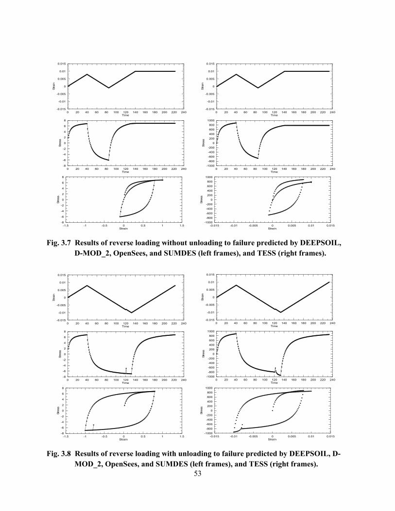
53

0 20 40 60 80 100 120 140 160 180 200 220 240Time

-0.015

-0.01

-0.005

0

0.005

0.01

0.015

Stra

in

0 20 40 60 80 100 120 140 160 180 200 220 240Time

-8

-6

-4

-2

0

2

4

6

8

Stre

ss

-1.5 -1 -0.5 0 0.5 1 1.5Strain

-8

-6

-4

-2

0

2

4

6

8

Stre

ss

0 20 40 60 80 100 120 140 160 180 200 220 240Time

-0.015

-0.01

-0.005

0

0.005

0.01

0.015

Stra

in

0 20 40 60 80 100 120 140 160 180 200 220 240Time

-1000

-800

-600

-400

-200

0

200

400

600

800

1000

Stre

ss

-0.015 -0.01 -0.005 0 0.005 0.01 0.015Strain

-1000

-800

-600

-400

-200

0

200

400

600

800

1000

Stre

ss

Fig. 3.7 Results of reverse loading without unloading to failure predicted by DEEPSOIL,

D-MOD_2, OpenSees, and SUMDES (left frames), and TESS (right frames).

0 20 40 60 80 100 120 140 160 180 200 220 240Time

-0.015

-0.01

-0.005

0

0.005

0.01

0.015

Stra

in

0 20 40 60 80 100 120 140 160 180 200 220 240Time

-8

-6

-4

-2

0

2

4

6

8

Stre

ss

-1.5 -1 -0.5 0 0.5 1 1.5Strain

-8

-6

-4

-2

0

2

4

6

8

Stre

ss

0 20 40 60 80 100 120 140 160 180 200 220 240Time

-0.015

-0.01

-0.005

0

0.005

0.01

0.015

Stra

in

0 20 40 60 80 100 120 140 160 180 200 220 240Time

-1000

-800

-600

-400

-200

0

200

400

600

800

1000

Stre

ss

-0.015 -0.01 -0.005 0 0.005 0.01 0.015Strain

-1000

-800

-600

-400

-200

0

200

400

600

800

1000

Stre

ss

Fig. 3.8 Results of reverse loading with unloading to failure predicted by DEEPSOIL, D-

MOD_2, OpenSees, and SUMDES (left frames), and TESS (right frames).

4 Key Issues in Nonlinear Ground Response Analysis

As discussed in Chapter 2, equivalent-linear analyses require the specification of well-

understood and physically meaningful input parameters (shear-wave velocity, unit weight,

modulus reduction, and damping), while nonlinear ground response analyses often require the

specification of poorly understood parameters (such as viscous damping) that may or may not be

clearly associated with measurable soil properties. Previous studies have thoroughly investigated

the sensitivity of site response results to the equivalent-linear parameters (e.g., Roblee et al.

1996), but this level of understanding is not available for the nonlinear parameters. Moreover,

prior to this research, parameter selection criteria for many of those nonlinear parameters were

often poorly documented and were unavailable to users other than the code developers. This

situation has limited the application of nonlinear ground response analyses in engineering

practice (Kramer and Paulsen 2004). The objective of this chapter is to identify five key issues

that need to be understood to properly perform nonlinear ground response analyses. Several of

these issues are addressed directly in the chapter, while others are addressed in subsequent

chapters following detailed investigations to justify the recommendations that are provided. Most

of the material presented in this chapter was previously presented in Stewart et al. (2006) and

Stewart and Kwok (2008).

4.1 PARAMETERIZATION OF BACKBONE CURVE

4.1.1 Backbone Curve

Figure 4.1 shows a typical nonlinear backbone curve for a soil element, which has a hyperbolic

shape defined by the initial small-strain secant shear modulus (Gmax) and the shear strength (τff).

The classical definition of reference strain is the ratio γref = τff /Gmax (Hardin and Drnevich 1972).

The parametric description of the nonlinear backbone curve in the past has generally required the

56

specification of this reference strain along with a number of curve-fitting parameters. A practical

problem with this approach is that the shear strength at rapid strain rate, needed to define the

reference strain, is often not available. Another problem is that the shape of the backbone curve

at small strains, as established by hyperbolic models based on γref, may be inconsistent with

laboratory test data.

At least for problems involving low to moderate strain levels, a “pseudo-reference strain”

(γr) can be used in lieu of the strength-based reference strain. The term pseudo-reference strain is

used to avoid confusion with the reference strain as defined by Hardin and Drnevich (1972). The

pseudo-reference strain is defined from a laboratory modulus reduction curve as the shear strain

at which G/Gmax = 0.5. This definition arises from hyperbolic fits of G/Gmax curves according to

( )max1/

1 ar

G Gβ γ γ

=+

(4.1)

where β and a are fitting parameters generally taken as 1 and 0.92, respectively (Darendeli

2001). The advantages of using the pseudo-reference strain are that (1) γr can be readily

evaluated from the material-specific modulus reduction curves evaluated from laboratory testing

and (2) lacking material-specific testing, empirical relationships exist to predict γr as a function

of basic parameters such as PI, overburden stress, and overconsolidation ratio (Darendeli 2001;

Zhang et al. 2005).

Because pseudo-reference strains are determined from modulus reduction curves that are

typically defined for strains less than 1%, a backbone curve described by a hyperbolic curve fit

using γr would not necessarily be expected to accurately represent soil behavior at large strain,

including the shear strength. This problem is investigated by examining the degree to which the

shear strength implied by the use of Equation 4.1 (approximately Gmax × γr) is realistic. This is

done using ratios of Gmax to shear strength, for which empirical relationships are available from

Weiler (1988). The ratios from Weiler are for soils with OCR of 1–5, confining pressures σ =

100–500, kPa (1–5 tsf), and PI=15–45. Weiler’s undrained shear strengths (Su) are based on

direct simple shear testing. Weiler’s Gmax / Su ratio is compared to the inverse of Darendeli’s

(2001) estimate of γr (which is approximately the ratio of Gmax to the large-strain asymptote of

the hyperbolic curve, taken as shear strength).

As observed from Figure 4.2, the Gmax/effective-strength ratios implied by pseudo-

reference strain γr are significantly higher than those from Weiler for an overburden stress of σ

57

=100 kPa. This bias implies that the shear strength implied by γr is underestimated by

Darendeli’s relationships at σ = 100 kPa. This bias disappears at larger overburden pressures

(σ=500 kPa). Accordingly, at relatively shallow depths, the use of backbone curves derived from

the pseudo-reference strain parameter may overestimate the soil nonlinearity at large strains.

Recommendations for the evaluation of backbone curve parameters are given in a

subsequent section following a discussion of material damping.

Fig. 4.1 Schematic illustration of backbone curve used for nonlinear ground response

analyses.

Fig. 4.2 Comparison of Gmax / Su ratio from Weiler (1988) to inverse of pseudo-reference

strain (1/γr) from Darendeli (2001). Quantity 1/γr is approximately ratio of Gmax to shear strength implied by use of pseudo-reference strain for fitting nonlinear backbone curves.

58

4.1.2 Material Damping

Masing’s rules (Masing 1926) and extended Masing rules (Vucetic 1990; Pyke 1979) are

employed in nonlinear analysis in conjunction with the backbone curve to describe unloading,

reloading, and cyclic degradation behavior of soil. Material damping is directly proportional to

the area contained within a cyclic stress-strain loop, and hence is sensitive to the shape of the

backbone curve and unload/reload rules. The damping at large strain that results from the use of

Masing or extended Masing rules tends to be overestimated relative to laboratory measurements.

There are three schools of thought on managing the overestimation of damping. One

approach is to select model parameters for the backbone curve (and hence modulus reduction

curves) that optimally fit the target data and to accept the resulting overestimation of damping

using Masing’s rules. A second approach is to select model parameters that optimize the fitting

of modulus reduction and damping curves simultaneously (across the strain range of interest).

The third approach is to introduce an additional parameter that changes the shape of the

unload/reload curves so that both modulus reduction and damping curves can be fit

simultaneously. Lo Presti et al. (2006) allows unloading and reloading curves to have a shape

scaled from that of the backbone curve by a factor of n (for the original Masing criteria, n = 2).

Lo Presti et al. provides recommendations for estimating n as a function of soil type, strain level,

and number of cycles for the motion. Wang et al. (1980) suggest an approach in which a

damping correction factor is applied to the Masing rule damping. These unload/reload rules are

not yet implemented in the nonlinear codes considered in this study, which are the codes most

often used in engineering practice, and hence this approach is not discussed further. The relative

merits of the first two approaches were investigated using vertical array data, and the results of

that investigation are discussed in Chapter 7.

4.1.3 Parameter Selection for Backbone Curve and Damping

There are two basic elements to the specification of parameters describing the nonlinear

backbone curve and damping. The first element is to select the target shape of the backbone

curve (equivalently, the modulus reduction curve) and the damping curve. The second element is

to select model parameters that describe the target relationships within a reasonable degree of

approximation for the problem at hand. Following the discussion of each element below, we

59

present results of sensitivity studies illustrating the implications for the computed site response

of alternative parameter selection procedures.

Element (1)—Target Curves: The ideal characterization would involve material-specific cyclic

testing across the strain range of interest. This testing would include characterization of the

material’s dynamic shear strength for large-strain problems. However, material-specific testing is

usually not available, requiring the nonlinear behavior to be described using published

correlations relating soil index properties, stress state, and stress history to parameters describing

modulus reduction and damping curves (e.g., Darendeli 2001; Zhang et al. 2005). Those

relationships are usually well defined to shear strains of approximately 0.3–0.7%. This is

illustrated in Figure 4.3, which shows the modulus reduction-strain values in the database used

by Darendeli (2001). As described previously, these relationships do not typically provide an

adequate representation of the shear strength. Guidelines for undrained shear strength evaluation

and estimation are given in Ladd (1991); these estimates should be adjusted in consideration of

rate effects, as described for example by Sheahan et al. (1996).

G/G

max

Shear Strain (%) Fig. 4.3 Modulus-reduction-strain values in database used by Darendeli (2001).

For problems involving large-strain soil response, traditional practice has been to use a

hyperbolic stress-strain curve (Eq. 4.1) with the strength-based reference strain. However, as

shown in Figure 4.4, because of the misfit of the reference and pseudo-reference strains, this

approach provides a poor match to small-strain modulus reduction behavior from laboratory

tests. Accordingly, we recommend an alternative approach illustrated in Figure 4.4 and explained

60

in the following: (1) use cyclic test results or correlation relationships to define the shape of the

backbone curve to strain level γ1 (typically taken as 0.1–0.3%); (2) estimate the material shear

strength (τff) for simple shear conditions with appropriate adjustment for rate effects; (3) estimate

the modulus reduction ordinates between strain γ1 and the shear strength with the following

hyperbolic relationship:

1

1 1

1/1 ( ) / ff

G GGγ

γ γ γ τ=

+ −(applies for γ > γ1 only) (4.2)

where Gγ1=secant shear modulus from Step (1) at γ= γ1. An example application of this procedure

is given by Chiu et al. (2008). In some cases this procedure can produce a noticeable kink in the

modulus reduction curve, and additional smoothing is necessary to achieve a satisfactory result.

At present, only OpenSees allows the input of the G/Gmax curve ordinates so that this formulation

could be directly applied.

0.0001 0.001 0.01 0.1 1 10Shear Strain (%)

0

0.2

0.4

0.6

0.8

1

G/G

max

0.0001 0.001 0.01 0.1 1 10Shear Strain (%)

0

10

20

30

40Sh

ear S

tres

s (k

Pa) Ps. Ref. Strain

Ref. Strain with τff/σv'=0.28Adjusted

γ1 γ1

Fig. 4.4 Modulus reduction and stress-strain curves implied by pseudo-reference

strain from Darendeli (2001), reference strain model, and proposed procedure (PI=20, OCR=1, σv’= 100 kPa, Vs=135 m/s).

Element (2)—Approximation of Target Curves: As noted above, an exact match of target

curves is not possible when Masing rules or extended Masing rules are used to describe the

unload-reload relationship. Until nonlinear codes implement the capability to simultaneously

match both modulus reduction and damping curves, mismatch of one or both of these curves is

unavoidable. As mentioned previously, one approach is to match the target modulus reduction

curve as accurately as possible and accept the misfit of damping. Another is to optimize the fit of

both simultaneously.

61

We have worked with Hashash and Phillips (pers. comm. 2006) to devise a scheme to

search for model parameters to achieve the aforementioned fitting approaches (in addition, the

scheme allows optimization of the fitting of the damping curve only, although this approach is

usually not considered). The scheme requires the specification of target material curves at (user-)

predetermined strain levels. The fitting error is considered up to a maximum strain level (usually

between 0.1 and 1%). The best combination of model parameters would be the one that gives the

least error between the target curves and model curves. This error is quantified as:

max max

2 2/ /( ) ( )G G G Gw wβ βε ε ε= × + × (4.3)

where max/G Gε and βε represent the mean error for the fitting of modulus reduction and damping

curves, respectively. Error term max/G Gε is calculated as:

( )max

max

2

/

/

( )G G i

G G N

ε γε =

∑ (4.4)

The numerator in Equation 4.4 is the summation of fitting error from the lowest specified strain

level to the maximum strain level. N is the number of strain levels included in the summation.

Error term βε is calculated in a similar way as for max/G Gε . Terms

max/G Gw and wβ in Equation

4.3 are weight factors whose values depend on the choice of fitting approach. Table 4.1

summarizes the values of weight factors under different fitting approaches. Figure 4.5 shows

differences in the fitted modulus reduction and damping curves (relative to target data) when

different fitting approaches are employed.

Table 4.1 Weight criterion for different fitting approaches.

Fitting Approach Weight Criterion MR

max/ 1; 0G Gw wβ= = MRD

max

max

2 2/

max

/ maxmax

max

( ) ( ) 1

1, 25%0.251 , 10%< 25%

0.152, 10%

G G

G G

w w

ww

β

β

ββ β

β

+ =

>⎧⎪ −⎪= + <⎨⎪

<⎪⎩

D max/ 0; 1G Gw wβ= =

62

0.0001 0.001 0.01 0.1 1Cyclic Strain (%)

0

10

20

30

Dam

ping

(%)

0

0.2

0.4

0.6

0.8

1

G/G

max

Target - Lab DataOptimizing MR fit only("MR" Fit)Trade off between MR and damping fits("MRD" Fit)Optimizing damping only("D" Fit)

Fig. 4.5 Different approaches in fitting modulus reduction and damping curves in

nonlinear analysis.

Effect of Parameter Selection Procedures on Computed Response (Overview): To illustrate

the sensitivity of the computed site response to details of the parameter selection protocols, we

describe below the results of two suites of analysis. The first suite concerns the implications of

selecting alternative target nonlinear curves — the principle issue being the use of curves

constrained by shear strength (i.e., true reference strain) or not. The second suite concerns the

implications of alternative fitting procedures for a given set of target nonlinear curves.

Effect of Parameter Selection Procedures on Computed Response—(1) Alternative Target

Nonlinear Curves: As described above, it is possible to select parameters describing the

backbone curve so that misfit is minimized between the modulus reduction and damping

behavior represented by the soil model and target curves from laboratory testing. However, as

shown in Figure 4.2, there is a potential for significant underestimation of shear strength with

such approaches. Accordingly, utilization of the shear strength in the parameterization of the

backbone curves (e.g., by using the true reference strain) is often preferred for depth intervals

63

where very large strains are expected. In this section, we investigate the effect of backbone curve

characteristics at large strain on-site response. We specifically seek to answer two questions: (1)

What is the effect of underestimating shear strength through the use of pseudo-reference strain?

and (2) What is the effect on-site response of using the true reference strain, which accurately

captures large-strain behavior but produces a misfit in modulus reduction and damping curves at

small strains?

We seek to answer the above questions using nonlinear ground response analyses for the

Apeel 2 site, located in Redwood City, California, and has a soft clay layer near the ground

surface (Bay Mud). Large-strain response during strong shaking is expected in the Bay Mud

layer (3.4–8.8 m depth). Shear strengths for this layer are estimated using the SHANSEP method

(Ladd 1991). Bay Mud is assumed to be normally consolidated with a dynamic shear strength

ratio of su/σ’c = 0.32. As shown in Figures 4.6–4.7 (black curves), modulus reduction/damping,

and backbone curves for different depths within the Bay Mud are obtained using reference

strains calculated from su and β=a=1.0 (to enforce a limiting shear stress = su).

The results obtained using the above curves are compared to additional results obtained

by matching small-strain behavior. Pseudo-reference strain is estimated using two methods: (1)

based on recommendations by Darendeli’s (2001) for PI = 50, OCR=1.0, σ’ = 52–85 kPa for

modulus reduction, and allowing overestimation of damping (MR fitting) and (2) based on MRD

fitting (described in Section 4.2) in which γr and the fitting parameters are optimized to

simultaneously fit Darendeli’s modulus reduction and damping curves. Additional analyses are

performed using the hybrid approach illustrated in Figure 4.4 in which small-strain behavior is

matched to Darendeli (2001) and large-strain behavior is controlled by the shear strength. The

modulus reduction/damping and backbone curves obtained using these approaches are shown in

Figures 4.6 and 4.7, respectively. Figure 4.6 shows that the modulus reduction and damping

curves calculated from γr based on Darendeli’s method demonstrate more nonlinearity than those

based on γref. In addition, Figure 4.7 shows that the shear strength is underestimated by the use of

pseudo-reference strain, which is consistent with the results in Figure 4.2. With respect to MRD

fitting (using Darendeli’s curves as the target), the nonlinearity is reduced (Fig. 4.6) but the peak

shear stress is increased to a level that happens to roughly match the shear strength (Fig. 4.7).

This is accidental and will not generally be the case. In general, misfit of shear strength will

64

occur at large strains and therefore the MRD-fitting procedures, as currently formulated, should

be used only for relatively small strains (less than 1%).

Nonlinear ground response analyses are performed with the above four sets of backbone

curves (shear-strength based; Darendeli with MR fitting; Darendeli with MRD fitting; hybrid).

The input motion is the same broadband synthetic considered previously with scaling to PHAr =

0.05, 0.17 g, 0.68 g, and 1.0 g. Maximum strain and PGA profiles are plotted in Figures 4.8–4.11

and response spectra are compared in Figure 4.12.

We draw two principal conclusions from these results. The first has to do with

underestimating shear strength by using pseudo-reference strain with MR fitting. To investigate

this effect, we focus on results involving large-strain response which, as indicated in Figures

4.8–4.11, occurs for input PHAr levels of 0.17 g and above. For these high levels of shaking the

results using the hybrid approach are considered to be mostly nearly “correct” because they

accurately capture both small and large-strain behavior. As shown in Figure 4.12, the

underestimation of shear strength can significantly limit the ground surface accelerations, as

reflected by low spectral acceleration for periods less than about 2–5 sec (depending on the level

of shaking). We note that the MRD method also provides good results in this case because of the

(accidental) match of large-strain behavior. As noted previously, this will generally not be the

case.

The second conclusion that can be drawn from these results concerns the effect of misfit

of modulus reduction and damping curves at small and mid-level strains (< about 0.5%) by using

the true reference strain in defining the backbone curve. As before, results from the hybrid

approach (and to a lesser extent, the MRD approach) are taken as most nearly “correct” because

they provide the best fit to the modulus reduction and damping curves over a wide range of

strains. We note that the reference-strain-based approach overestimates the response, which we

interpret to result from the underestimation of damping. This is one potential drawback to the use

of true reference strain —relatively small-strain response could be biased, and this bias will tend

to be toward overprediction of response because damping will be lower than target levels (this

occurs because the G/Gmax curve is more linear).

The general recommendation is to use shear strength data in the development of

backbone curves when large-strain response is anticipated. This can be done in two ways. The

first is to use Equation 4.1 with the true reference strain (su/Gmax using measured shear strengths)

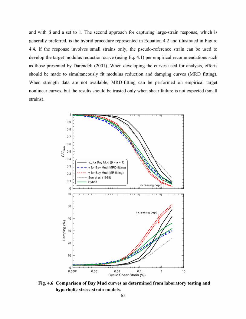
65

and with β and a set to 1. The second approach for capturing large-strain response, which is

generally preferred, is the hybrid procedure represented in Equation 4.2 and illustrated in Figure

4.4. If the response involves small strains only, the pseudo-reference strain can be used to

develop the target modulus reduction curve (using Eq. 4.1) per empirical recommendations such

as those presented by Darendeli (2001). When developing the curves used for analysis, efforts

should be made to simultaneously fit modulus reduction and damping curves (MRD fitting).

When strength data are not available, MRD-fitting can be performed on empirical target

nonlinear curves, but the results should be trusted only when shear failure is not expected (small

strains).

0

0.1

0.2

0.3

0.4

0.5

0.6

0.7

0.8

0.9

1

G/G

max

γref for Bay Mud (β = a = 1)

γr for Bay Mud (MRD fitting)

γr for Bay Mud (MR fitting)Sun et al. (1988)Hybrid

0.0001 0.001 0.01 0.1 1 10Cyclic Shear Strain (%)

0

10

20

30

40

50

60

Dam

ping

(%)

increasing depth

increasing depth

Fig. 4.6 Comparison of Bay Mud curves as determined from laboratory testing and

hyperbolic stress-strain models.

66

0 1 2 3 4 5 6 7 8 9 10Shear Strain (%)

0

10

20

30

40

She

ar S

tress

(kP

a)

γref for Bay Mud (β = a = 1)

γr for Bay Mud (MRD Fitting)

γr for Bay Mud (MR Fitting)Hybrid

increasing depth

Fig. 4.7 Stress-strain curve as implied by different reference and pseudo-reference strain

values.

0 100 200 300 400 500 600Vs (m/sec)

100

80

60

40

20

0

Dep

th (m

)

0 0.2 0.4 0.6 0.8PGA (g)

0.01 0.1 1Maximum Shear Strain (%)

PHAr = 0.05gγref for Bay Mud (β = a = 1)

γr for Bay Mud (MRD fitting)


Fig. 4.8 Maximum strain and PGA profiles for PHAr=0.05 g from nonlinear analyses.

67

0 100 200 300 400 500 600Vs (m/sec)

100

80

60

40

20

0

Dep

th (m

)

0 0.2 0.4 0.6 0.8PGA (g)



γr for Bay Mud (MRD fitting)γr for Bay Mud (MR Fitting)Hybrid


0 100 200 300 400 500 600Vs (m/sec)

100

80

60

40

20

0

Dep

th (m

)

0 0.2 0.4 0.6 0.8PGA (g)



γr for Bay Mud (MRD fitting)γr for Bay Mud (MR Fitting)Hybrid


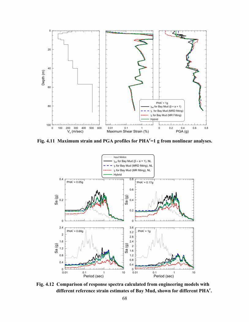
68

0 100 200 300 400 500 600Vs (m/sec)

100

80

60

40

20

0

Dep

th (m

)

0 0.2 0.4 0.6 0.8PGA (g)


PHAr = 1gγref for Bay Mud (β = a = 1)γr for Bay Mud (MRD fitting)


Fig. 4.11 Maximum strain and PGA profiles for PHAr=1 g from nonlinear analyses.

0

0.2

0.4

0.6

0.8

Sa

(g)

Input Motion

γref for Bay Mud (β = a = 1), NLγr for Bay Mud (MRD fitting), NL

γr for Bay Mud (MR fitting), NLHybrid

PHAr = 0.17g

0.01 0.1 1 10Period (sec)

0

0.4

0.8

1.2

1.6

2

2.4

Sa (g

)

PHAr = 0.68g

0.01 0.1 1 10Period (sec)

0

0.4

0.8

1.2

1.6

2

2.4

2.8

3.2

3.6

Sa

(g)

PHAr = 1g

0

0.2

0.4

Sa (g

)

PHAr = 0.05g

Fig. 4.12 Comparison of response spectra calculated from engineering models with

different reference strain estimates of Bay Mud, shown for different PHAr.

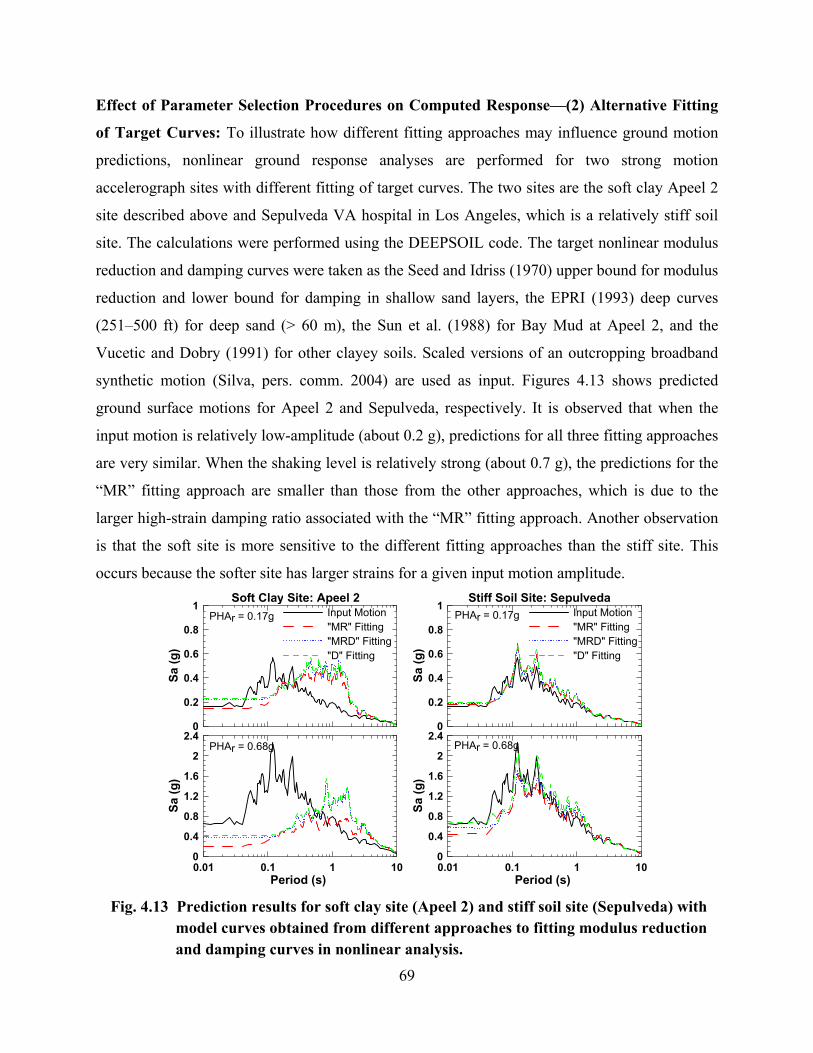
69

Effect of Parameter Selection Procedures on Computed Response—(2) Alternative Fitting

of Target Curves: To illustrate how different fitting approaches may influence ground motion

predictions, nonlinear ground response analyses are performed for two strong motion

accelerograph sites with different fitting of target curves. The two sites are the soft clay Apeel 2

site described above and Sepulveda VA hospital in Los Angeles, which is a relatively stiff soil

site. The calculations were performed using the DEEPSOIL code. The target nonlinear modulus

reduction and damping curves were taken as the Seed and Idriss (1970) upper bound for modulus

reduction and lower bound for damping in shallow sand layers, the EPRI (1993) deep curves

(251–500 ft) for deep sand (> 60 m), the Sun et al. (1988) for Bay Mud at Apeel 2, and the

Vucetic and Dobry (1991) for other clayey soils. Scaled versions of an outcropping broadband

synthetic motion (Silva, pers. comm. 2004) are used as input. Figures 4.13 shows predicted

ground surface motions for Apeel 2 and Sepulveda, respectively. It is observed that when the

input motion is relatively low-amplitude (about 0.2 g), predictions for all three fitting approaches

are very similar. When the shaking level is relatively strong (about 0.7 g), the predictions for the

“MR” fitting approach are smaller than those from the other approaches, which is due to the

larger high-strain damping ratio associated with the “MR” fitting approach. Another observation

is that the soft site is more sensitive to the different fitting approaches than the stiff site. This

occurs because the softer site has larger strains for a given input motion amplitude.

0

0.2

0.4

0.6

0.8

1

Sa (g

)

Soft Clay Site: Apeel 2Input Motion"MR" Fitting"MRD" Fitting"D" Fitting

PHAr = 0.17g

0.01 0.1 1 10Period (s)

0

0.4

0.8

1.2

1.6

2

2.4

Sa (g

)

PHAr = 0.68g

0

0.2

0.4

0.6

0.8

1

Sa (g

)

Stiff Soil Site: SepulvedaInput Motion"MR" Fitting"MRD" Fitting"D" Fitting

PHAr = 0.17g

0.01 0.1 1 10Period (s)

0

0.4

0.8

1.2

1.6

2

2.4

Sa (g

)

PHAr = 0.68g

Fig. 4.13 Prediction results for soft clay site (Apeel 2) and stiff soil site (Sepulveda) with

model curves obtained from different approaches to fitting modulus reduction and damping curves in nonlinear analysis.

70

4.2 LIMITATION IN LAYER THICKNESS

The maximum frequency of a layer is the highest frequency that the layer can propagate and is

calculated as Vs/4H (Vs and H are the shear wave velocity and thickness of the layer,

respectively) which corresponds to the fundamental frequency of the soil layer. If a layer is too

thick the maximum frequency that a layer can propagate would be small. Figure 4.14 compares

the predicted response spectra using different numbers of layers in modeling the Gilroy 2 with a

broadband synthetic motion provided by Silva (pers. comm. 2004). It can be seen that using

fewer layers (hence thicker layers) would result in lower pseudo spectral accelerations especially

at small periods as the high-frequency waves are filtered out. This issue is often not addressed in

the user’s manuals of nonlinear ground response analysis codes. Therefore, it is necessary to

improve the manuals by reminding users of the importance of checking the maximum frequency

of each layer. The most commonly used maximum frequency is 25 Hz.

0.01 0.1 1 10Period (sec)

0

0.1

0.2

0.3

0.4

0.5

0.6

Sa

(g)

Input Motion 25 layers49 layers

5% Damping

Fig. 4.14 Predicted response spectra computed using different numbers of layer.

4.3 SPECIFICATION OF INPUT MOTION

Input motions are specified at the bottom of the 1D site profile in nonlinear analyses. There has

been confusion regarding whether the motions specified at the base of the profile should

represent an outcropping condition (i.e., equivalent free-surface motions that are twice the

amplitude of the incident wave due to full reflection) or a within condition (i.e., the sum of the

71

incident waves and downward propagating waves reflected from overlying layer interfaces). A

closely related question is whether the base condition (representing the material below the site

column) should be elastic or rigid. This issue is addressed by using exact solutions of wave

propagation problems for elastic conditions in Chapter 5.

4.4 SPECIFICATION OF VISCOUS DAMPING

As discussed in Chapter 3, most nonlinear codes use some form of viscous damping to provide

for damping in the analysis at very small strains where the hysteretic damping from the nonlinear

soil models is nearly zero (an exception is TESS, which does not require viscous damping and

has a low strain damping scheme). Few protocols are available for guiding the selection of an

appropriate viscous damping scheme. In Chapter 5, guidelines on this issue are developed by

using exact solutions of wave propagation problems for elastic conditions.

5 Verification of Nonlinear Codes against Exact Solutions

5.1 INTRODUCTION

In this chapter, two key issues related to the practical application of nonlinear ground response

analysis codes are resolved by comparing the results of such analyses (under linear condition) to

known theoretical solutions. These two issues are the specification of input motions as

“outcropping” (i.e., equivalent free-surface motions) versus “within” (i.e., motion occurring at a

depth within a site profile), and the specification of the damping that occurs within a soil element

at small strains, which is either accomplished using viscous damping or unload-reload rules that

produce non-zero small-strain hysteretic damping. The five nonlinear seismic ground response

analysis codes discussed in Chapter 2 (D-MOD_2, DEEPSOIL, TESS, OpenSees, and

SUMDES) are considered in the analyses.

The chapter begins with a brief review of the solution characteristics in the frequency-

domain and time-domain ground response analysis procedures. This is followed by sections

describing verification studies addressing the issues of input motion specification and modeling

of small-strain damping. The content of this chapter also appears in a journal paper by Kwok et

al. (2007).

5.2 ONE-DIMENSIONAL GROUND RESPONSE ANALYSIS PROCEDURES

In 1D seismic ground response analyses, soil deposits are assumed to be horizontally layered

over a uniform halfspace. The incident wave is assumed to consist of vertically propagating

shear waves. The response of a soil deposit to the incident motion can be modeled in the

frequency or time domains, as described below.

74

5.2.1 Frequency-Domain Analysis

Frequency-domain analyses are based on a closed-form solution of the wave equation for shear

wave propagation through a layered continuous medium, with each layer i having a specified

density ρi, shear modulus Gi, and hysteretic damping βi. The solution was presented by Roesset

and Whitman (1969), Lysmer et al. (1971), Schnabel et al. (1972), and is also described in detail

by Kramer (1996). In these frequency-domain methods, a control motion of frequency ω is

specified at any layer j in the system. An exact solution of the system response can be expressed

as a transfer function relating the sinusoidal displacement amplitude in any arbitrary layer i to the

amplitude in layer j,

( ) ( )( ) ( )ωω

ωωjj

iiij ba

baF

++

= (5.1)

where Fij = amplitude of transfer function between layers i and j, ai and aj = normalized

amplitudes of upward propagating waves in layers i and j, and bi and bj = normalized amplitudes

of downward propagating waves in layers i and j. The normalization of the wave amplitudes is

generally taken relative to the amplitude in layer 1, for which a1 = b1 due to perfect wave

reflection at the free surface. The normalized amplitudes ai, aj, bi, and bj can be computed from a

closed-form solution of the wave equation, and depend only on profile characteristics (i.e.,

material properties ρ, G, and β for each layer and individual layer thicknesses).

The frequency-domain solution operates by modifying, relative to the control motion, the

wave amplitudes in any layer i for which results are required. These analyses are repeated across

all the discrete frequencies for which a broadband control motion is sampled, using the fast

Fourier transform. Once amplitudes ai and bi have been computed for a given layer at all these

frequencies, time-domain displacement histories of layer i can be calculated by an inverse

Fourier transformation.

Control motions for use in frequency-domain analyses are most often recorded at the

ground surface and are referred to as “outcropping.” As perfect wave reflection occurs at the

ground surface, incident and reflected wave amplitudes are identical, and hence outcropping

motions have double the amplitude of incident waves alone. Consider the example in Figure 5.1.

Rock layer n occurs at the base of a soil column in Case 1 and as outcropping rock in Case 2. In

the outcropping rock case, incident and reflected waves are equivalent (an* = bn*). The incident

waves are identical in both cases (an* = an), assuming equal rock moduli, but the reflected waves

75

differ (bn* ≠ bn) because some of the incident wave transmits into the soil (nonperfect reflection)

for Case 1, whereas perfect reflection occurs in Case 2. The motion at the base of the soil column

in Case 1 (referred to as a “within” motion) can be evaluated from the outcropping motion using

the transfer function:

( ) ( )( )ω

ωωn

nn

n

nnn a

bauu

F2**

+== (5.2)

As with any other transfer function, Fnn* can be readily computed for any frequency ω and

depends only on profile characteristics. Accordingly, through the use of Equation 5.2, the within

motion can be calculated for a given outcropping motion. The base-of-profile (within) motion

can in turn be used to calculate motions at any other layer per Equation 5.1.

an* bn*an bn

CASE 1: Soil over rock CASE 2: Outcropping rock Fig. 5.1 Incident and reflected waves in base rock layer for case of soil overlying rock and

outcropping rock (amplitudes shown are relative to unit amplitude in Case 1 surface layer).

The application of Equation 5.2 results in a within motion that is reduced from an

outcropping motion at the site (modal) frequencies. Consider, for example, a single soil layer

with thickness = 30 m, Vs = 300 m/s [giving a fundamental mode site frequency of fs = (300 m/s

)/ (4×30 m) = 2.5 Hz] overlying a halfspace with shear wave velocity Vs-H. The results of the

within/outcropping calculation (i.e., Eq. 5.2) are shown in Figure 5.2a for various values of

equivalent viscous damping ratio (equal damping values are applied in both the soil layer and

halfspace) with Vs-H=2Vs and in Figure 5.2b for zero damping and various levels of velocity

contrast (Vs/Vs-H). As shown in Figure 5.2 (a and b), the transfer function amplitude

(within/outcropping) drops below unity near the site frequencies, with the amplitudes at site

frequencies decreasing only with decreasing amounts of equivalent viscous damping. At

frequencies between the site frequencies, amplitudes decrease both with increasing damping and

with decreasing velocity contrast.

76

At zero damping the transfer function amplitude goes to zero at site frequencies. To

understand this phenomenon, consider that (1) control motion and response are in phase in this

case because of the lack of damping and (2) the site frequencies correspond to 2n+1 quarter wave

lengths, where n = 0, 1, 2, etc. (zero and positive integers). As shown in Figure 5.2c, at a depth

below the surface of 2n+1 quarter-wave lengths, the wave amplitude is zero (i.e., there is a

“node” in the response at that depth), which in turn must produce a zero transfer function

amplitude (Fig. 5.2c shows mode shapes for the 1st and 3rd modes, i.e., n=0 and 1). Additionally,

as shown in Figure 5.2c (lower right frame), as damping increases, the input and response are

increasingly out of phase, and there are no true nodes in the site response.

0

0.2

0.4

0.6

0.8

1

1.2

With

in/O

utcr

oppi

ng

Am

plitu

de

β=0%β=1%β=5%β=10%

0 1 2 3 4 5 6 7 8f / fs

0

0.2

0.4

0.6

0.8

1

1.2

With

in/O

utcr

oppi

ngA

mpl

itude

Vs-H=2Vs

Vs-H=5Vs

Vs-H=10Vs

Vs-H=20Vs

Vs-H = 2 Vs

β = 0%

Dep

th

Surface

H

Vs

Vs-H

Dep

th

uβ=0

0

Dep

th

0

β>0

β=0

u

3rd mode

1st mode 1st mode

(a)

(b)

(c)

Fig. 5.2 Ratio of within to outcropping amplitudes for (a) various equivalent viscous

damping ratios; (b) various base layer velocities (Vs-H); and (c) mode shapes for various conditions.

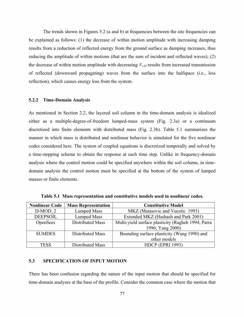
77

The trends shown in Figures 5.2 (a and b) at frequencies between the site frequencies can

be explained as follows: (1) the decrease of within motion amplitude with increasing damping

results from a reduction of reflected energy from the ground surface as damping increases, thus

reducing the amplitude of within motions (that are the sum of incident and reflected waves); (2)

the decrease of within motion amplitude with decreasing Vs-H results from increased transmission

of reflected (downward propagating) waves from the surface into the halfspace (i.e., less

reflection), which causes energy loss from the system.

5.2.2 Time-Domain Analysis

As mentioned in Section 2.2, the layered soil column in the time-domain analysis is idealized

either as a multiple-degree-of-freedom lumped-mass system (Fig. 2.3a) or a continuum

discretized into finite elements with distributed mass (Fig. 2.3b). Table 5.1 summarizes the

manner in which mass is distributed and nonlinear behavior is simulated for the five nonlinear

codes considered here. The system of coupled equations is discretized temporally and solved by

a time-stepping scheme to obtain the response at each time step. Unlike in frequency-domain

analysis where the control motion could be specified anywhere within the soil column, in time-

domain analysis the control motion must be specified at the bottom of the system of lumped

masses or finite elements.

Table 5.1 Mass representation and constitutive models used in nonlinear codes.

Nonlinear Code Mass Representation Constitutive Model D-MOD_2 Lumped Mass MKZ (Matasovic and Vucetic 1993) DEEPSOIL Lumped Mass Extended MKZ (Hashash and Park 2001) OpenSees Distributed Mass Multi-yield surface plasticity (Ragheb 1994; Parra

1996; Yang 2000) SUMDES Distributed Mass Bounding surface plasticity (Wang 1990) and

other models TESS Distributed Mass HDCP (EPRI 1993)

5.3 SPECIFICATION OF INPUT MOTION

There has been confusion regarding the nature of the input motion that should be specified for

time-domain analyses at the base of the profile. Consider the common case where the motion that

78

is to be applied was recorded at the surface of a rock site (outcrop motion). One school of

thought that has been applied in practice for many years is that the outcropping motion should be

converted to a within motion using frequency-domain analysis (e.g., Eq. 5.2), and that this within

motion should then be specified for use at the base of the site profile for application in time-

domain analysis. Most users of this approach were aware that the layer properties used in the

outcropping-to-within conversion were a potentially crude approximation to the actual nonlinear

soil properties. The approximation was accepted, however, due to the lack of a practical

alternative for obtaining within motions. The second school of thought is that the outcropping

rock motion should be applied directly at the base of the site profile without modification.

Normally, this direct use of the outcropping motion is accompanied by the use of a compliant

base in the site profile (the base stiffness being compatible with the character of the underlying

rock), which allows some of the energy in the vibrating soil deposit to radiate down into the

halfspace (Joyner and Chen 1975). Rigid base options are also available in all time-domain codes

but are seldom used because the conditions under which the rigid base should be applied are

poorly understood.

To evaluate which of the two above approaches is correct, time-domain analyses with

elastic material properties are exercised, for which frequency-domain analyses provide an exact

solution. This can be investigated using linear analyses because the underlying issue involves the

differences in linear wave propagation modeling with frequency-domain and time-domain

analyses. Consider for example a single soil layer with thickness = 30 m and a shear wave

velocity Vs = 300 m/s (site frequency = 2.5 Hz) that overlies an elastic halfspace with Vs-H = 2 Vs

= 600 m/s. Equivalent viscous damping is assumed constant at 5%. A control motion is selected

to represent an extreme scenario with respect to the variability between outcropping and within,

which is a sine wave at the site frequency. As shown in Figure 5.3c, the particular motion

selected has a frequency of 2.5 Hz, 12 cycles of shaking, and cosine tapers at the beginning and

end of the signal with a four-cycle taper duration (the tapers have the shape of half a cosine

wavelength). The control motion is specified for an outcropping condition. A large suppression

of the within motion relative to the outcropping motion would be expected for this signal (e.g., as

suggested by Fig. 5.2).

79

0 0.5 1 1.5 2 2.5 3 3.5 4 4.5 5 5.5 6 6.5 7Time (s)

-0.3

-0.2

-0.1

0

0.1

0.2

0.3

Inpu

t Out

crop

ping

A

ccel

erat

ion

(g)

-0.3

-0.2

-0.1

0

0.1

0.2

0.3

With

in M

otio

n fro

m S

HAK

E04

(g)

-0.3

-0.2

-0.1

0

0.1

0.2

0.3S

urfa

ce A

ccel

erat

ion

(g)

SHAKE04 Nonlinear Code (Outcropping Motion as Input + Elastic Base)Nonlinear Code (Within Motion as Input + Elastic Base)Nonlinear Code (Within Motion as Input + Rigid Base)Nonlinear Code (Outcropping Motion as Input + Rigid Base)

Frequency = 2.5 Hz

(a)

(b)

(c)

Fig. 5.3 Acceleration histories for one-layer problem.

A frequency-domain solution is exact because the material properties are elastic (i.e.,

strain-invariant). The frequency-domain calculations are performed with the computer program

SHAKE04 (Youngs 2004), which is a modified version of the original SHAKE program

(Schnabel et al. 1972). Both the within motion and the motion at the surface of the soil layer are

calculated, with the results shown in Figure 5.3 (a and b) with the solid black lines.

Linear time-domain analyses are performed for this site using the “nonlinear” codes listed

80

in Table 5.1 (the codes are implemented with linear backbone curves). Four combinations of

control motion and base condition are considered:

1. Outcropping motion (Fig. 5.3c) with elastic base (Vs-H = 600 m/s).

2. Within motion (which is extracted from frequency-domain analysis, see Fig. 5.3b) with

elastic base.

3. Outcropping motion with rigid base (Vs-H = 30000 m/s or select the “rigid base” option in

nonlinear code, if available).

4. Within motion with rigid base.

The results in Figure 5.3a show that the surface acceleration histories for cases (1) and (4) match

the known solution from frequency-domain analysis. Using the within motion with an elastic

base (Case 2) underestimates the surface motions, while using the outcropping motion with a

rigid base (Case 3) overestimates the surface motions.

Based on the above, our recommendations are as follows: (1) for the common case in

which the control motion is recorded as outcropping, the motion should be applied without

modification for time-domain analyses with an elastic base and (2) if time-domain analyses are

to be used to simulate the response of a vertical array using a control motion recorded at depth

within the site, the “within” motion should be used without modification in conjunction with a

rigid base.

5.4 MODELING OF DAMPING IN NONLINEAR TIME-DOMAIN ANALYSES

In nonlinear time-domain response models, there are generally two sources of damping. One

source is hysteretic damping (frequency independent) associated with the area bounded by

hysteretic stress-strain loops. When Masing (Masing 1926) and extended Masing rules (Pyke

1979; Wang et al. 1980; Vucetic 1990) are used to represent the unload-reload behavior of soil,

zero damping is encountered at small strains, where the backbone curve is linear. The zero

damping condition is incompatible with soil behavior measured in the laboratory at small strains

(e.g., Vucetic et al. 1998; Darendeli 2001) and can result in overestimation of propagated ground

motion. One solution to this problem is to add velocity-proportional viscous damping in the form

of dashpots embedded within the material elements depicted in Figure 2.3 (this approach is used

by DMOD_2, DEEPSOIL, OpenSees, and SUMDES). An alternative approach is to introduce a

81

scheme that produces non-zero hysteretic damping at small strains (e.g., TESS). It should be

noted that the nature of soil damping at small strains is neither perfectly hysteretic nor perfectly

viscous (Vucetic and Dobry 1986; Lanzo and Vucetic 1999). The incorporation of hysteretic or

viscous damping schemes into nonlinear codes is merely a convenient approximation for

simulation purposes and is required to ensure numerical stability of lumped-mass solutions.

5.4.1 Viscous Damping

There are a number of options for modeling viscous damping, which vary by code (Table 5.2).

As illustrated in Figure 5.4, there are three principal issues: (1) the form of the damping

formulation (simplified versus full or extended Rayleigh damping; Hashash and Park 2002); (2)

the target viscous damping ratio (labeled ζtar in Fig. 5.4) that is matched at specified target

frequencies; and (3) the matching frequencies (one, two, and four for the cases of simplified, full,

and extended Rayleigh damping, respectively).

Table 5.2 Available viscous damping formulation for nonlinear codes and summary of analyses discussed in text.

Nonlinear Code

Rayleigh Damping Option

Rayleigh Damping Option Considered in Current Analyses

Best Match to Frequency-

Domain Solution for all Three Sites

D-MOD_2 Simplified & Full Simplified (fsa; fma; fpa) ζtar=0.5% & 5%

Full (fs + 3×fs; fs + 5×fs) ζtar=0.5% & 5%

Full (5×fs) at ζtar=5%

DEEPSOIL Simplified, Full & Extended

Simplified (fs; fm; fp) ζtar=0.5% & 5%



OpenSees Simplified & Full Simplified (fs; fm; fp) ζtar=0.5% & 5%



SUMDES Simpified (Assuming damping ratio given at 1

Hz)b

Simplified (ζf = 5%/fs; 5%/fp; 1%/ fp; 1%) ζf = 1%

TESS No viscous damping a fs, fm, and fp represent site frequency, mean frequency, and predominant frequency of motion, respectively. b Any damping ratio at a desired frequency (e.g., fs) can be converted to damping ratio at 1 Hz using simple proportionality (e.g., ζf = ζfs /fs)

82

Visc

ous

Dam

ping

Rat

io

Frequencyf1 f2 f3 f4

Simplified Rayleigh Damping

Extended RayleighDamping

Full Rayleigh Damping

ζtar

Fig. 5.4 Schematic illustration of viscous damping models and model parameters (after

Park and Hashash 2004).

Few formal protocols are available to guide users in the selection of the Rayleigh

damping model type and parameters described above. With regard to the form of the damping

formulation, most practitioners use simplified or full Rayleigh damping. Extended Rayleigh

damping is seldom applied in practice. There are two schools of thought on the target damping

level (ζtar), which in practice is either taken as the small-strain damping or as the smallest

numerical value that appears to provide a stable solution in the judgment of the analyst (e.g., the

SUMDES manual suggests 0.02%–1%). With regard to matching frequencies, the lower target

frequency is generally taken as the site fundamental frequency. The larger target frequency is

generally taken as an odd-integer multiplier of the fundamental frequency (e.g., 3, 5, 7) (Hudson

et al. 1994).

An alternative set of guidelines was presented by Park and Hashash (2004), in which the

model parameters are selected through an iterative process in which frequency and time-domain

elastic solutions are matched within a reasonable degree of tolerance over a frequency range of

interest. The procedure is implemented through a user interface in the code DEEPSOIL but is

unavailable for other codes.

In the following, we develop recommended procedures for the specification of Rayleigh

damping that are intended to resolve some of the ambiguities in current practice with respect to

the three aforementioned issues (formulation, target damping, target frequencies). Such

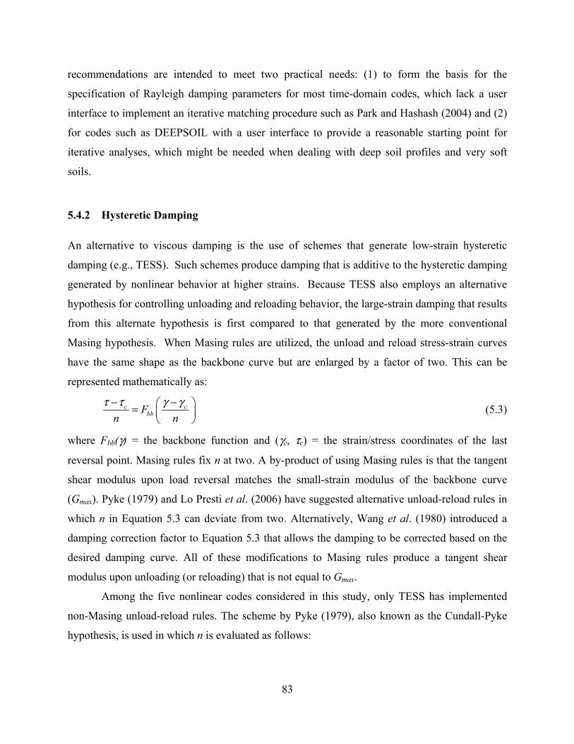
83

recommendations are intended to meet two practical needs: (1) to form the basis for the

specification of Rayleigh damping parameters for most time-domain codes, which lack a user

interface to implement an iterative matching procedure such as Park and Hashash (2004) and (2)

for codes such as DEEPSOIL with a user interface to provide a reasonable starting point for

iterative analyses, which might be needed when dealing with deep soil profiles and very soft

soils.

5.4.2 Hysteretic Damping

An alternative to viscous damping is the use of schemes that generate low-strain hysteretic

damping (e.g., TESS). Such schemes produce damping that is additive to the hysteretic damping

generated by nonlinear behavior at higher strains. Because TESS also employs an alternative

hypothesis for controlling unloading and reloading behavior, the large-strain damping that results

from this alternate hypothesis is first compared to that generated by the more conventional

Masing hypothesis. When Masing rules are utilized, the unload and reload stress-strain curves

have the same shape as the backbone curve but are enlarged by a factor of two. This can be

represented mathematically as:

c cbbF

n nτ τ γ γ− −⎛ ⎞= ⎜ ⎟

⎝ ⎠ (5.3)

where Fbb(γ) = the backbone function and (γc, τc) = the strain/stress coordinates of the last

reversal point. Masing rules fix n at two. A by-product of using Masing rules is that the tangent

shear modulus upon load reversal matches the small-strain modulus of the backbone curve

(Gmax). Pyke (1979) and Lo Presti et al. (2006) have suggested alternative unload-reload rules in

which n in Equation 5.3 can deviate from two. Alternatively, Wang et al. (1980) introduced a

damping correction factor to Equation 5.3 that allows the damping to be corrected based on the

desired damping curve. All of these modifications to Masing rules produce a tangent shear

modulus upon unloading (or reloading) that is not equal to Gmax.

Among the five nonlinear codes considered in this study, only TESS has implemented

non-Masing unload-reload rules. The scheme by Pyke (1979), also known as the Cundall-Pyke

hypothesis, is used in which n is evaluated as follows:

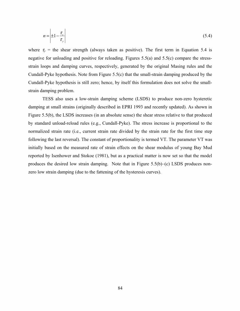
84

1 c

y

n ττ

= ± − (5.4)

where τy = the shear strength (always taken as positive). The first term in Equation 5.4 is

negative for unloading and positive for reloading. Figures 5.5(a) and 5.5(c) compare the stress-

strain loops and damping curves, respectively, generated by the original Masing rules and the

Cundall-Pyke hypothesis. Note from Figure 5.5(c) that the small-strain damping produced by the

Cundall-Pyke hypothesis is still zero; hence, by itself this formulation does not solve the small-

strain damping problem.

TESS also uses a low-strain damping scheme (LSDS) to produce non-zero hysteretic

damping at small strains (originally described in EPRI 1993 and recently updated). As shown in

Figure 5.5(b), the LSDS increases (in an absolute sense) the shear stress relative to that produced

by standard unload-reload rules (e.g., Cundall-Pyke). The stress increase is proportional to the

normalized strain rate (i.e., current strain rate divided by the strain rate for the first time step

following the last reversal). The constant of proportionality is termed VT. The parameter VT was

initially based on the measured rate of strain effects on the shear modulus of young Bay Mud

reported by Isenhower and Stokoe (1981), but as a practical matter is now set so that the model

produces the desired low strain damping. Note that in Figure 5.5(b)–(c) LSDS produces non-

zero low strain damping (due to the fattening of the hysteresis curves).

85

Fig. 5.5 Comparison of stress-strain loops generated from (a) Masing rules and Cundall-

Pyke hypothesis; (b) Cundall-Pyke hypothesis with and without the low-strain damping scheme (LSDS); and (c) comparison of damping curves generated from different schemes.

5.5 VALIDATION AGAINST KNOWN THEORETICAL ELASTIC SOLUTIONS

Validation is performed by comparing results of linear time-domain analyses performed with

alternative specifications of damping (viscous or LSDS) to an exact solution from linear

frequency-domain analyses. The frequency-domain analyses are exact because of the use of

linear soil properties and frequency-independent damping. This issue can be investigated using

86

linear analyses because the problem is associated with small-strain conditions at which soil

behavior is practically linear. The analyses are conducted for three selected sites that represent a

broad range of site conditions: shallow stiff soil over rock, soft clay overlying stiffer sediments

and rock, and very deep stiff soils typical of the Los Angeles basin (site frequencies range from

0.45–6.4 Hz). The control motion is a broadband synthetic acceleration history calculated for an

outcropping rock site condition (motion provided by Dr. Walter Silva, pers. comm. 2004).

Similar results were obtained when other control motions were utilized. The equivalent viscous

damping ratio used in the frequency-domain analysis is 5% for all layers. For the time-domain

codes D-MOD_2, DEEPSOIL, and OpenSees, target damping ratios of 0.5% and 5% are used to

evaluate whether the target viscous damping ratio should match the small-strain material

damping or a much smaller value. Both simplified and full Rayleigh damping formulations are

used for these three codes (see Table 5.2 for details).

For SUMDES, only simplified Rayleigh damping was available at the time this report

was written (implementation of full Rayleigh damping is in progress), and the SUMDES manual

calls for the target damping ratio to be specified at 1 Hz (Li et al. 1992). Past practice has been

that the 1 Hz damping (ζf1) is scaled from the target damping level (ζtar, e.g., 5%) at some

specified frequencies (often the predominant frequency of the input motion, fp) as

ptarf fςς =1 (5.5)

For SUMDES analyses, we use a 5% target damping level with matching frequencies at fp

(predominant frequency ≡ frequency having maximum spectral acceleration) and fs (elastic site

frequency). We also use a 1% target damping level with a matching frequency of fp. Finally, we

use a fixed damping ratio of ζf1 = 1%. These options are summarized in Table 5.2.

For TESS it is recommended that the numerical value of the parameter VT be set to equal

the desired low strain damping ratio, 0.05 in this case. As indicated in Table 5.2, we also utilize

values of 0.01 and 0.10 to test the sensitivity of the computed results to VT and hence to the

amount of hysteretic damping that is introduced.

5.5.1 Shallow Stiff Site: Simi Valley Knolls School

The upper 14 m of Simi Valley Knolls School is composed of silty sand, which has shear wave

velocities of about 300 m/s and is underlain by sandstone (site frequency fs = 6.4 Hz). Figures 5.6

87

and 5.7 compare 5% damped acceleration response spectra of surface motions from the

frequency-domain solution (developed using SHAKE04; Youngs 2004) with time-domain results

from the five codes listed in Table 5.2.

The trends in the D-MOD_2, DEEPSOIL, and OPENSEES results are similar.

Comparing the left and right frames, the results are somewhat better for the 5% target damping

ratio, but are relatively insensitive to the damping for this shallow site. Both simplified and full

Rayleigh damping formulations are reasonably effective, although simplified Rayleigh damping

with the target frequency set to the mean frequency of the input motion overdamps the computed

response at short periods (the site frequency is a preferred target).

For SUMDES, the results in Figure 5.7 show that a target damping ratio of 5% produces

overdamping at high frequencies regardless of the matching frequency (fp or fs), whereas ζtar=1%

provides a slightly improved fit. However, the results for all the different damping formulations

fall within a narrow range for this shallow stiff site. For TESS, results are shown for three values

of VT. The best fit is obtained by using values of VT that are one or two times the viscous

damping ratio from frequency-domain analysis.

88

0

0.2

0.4

0.6

0.8

1

1.2

1.4

1.6

1.8Ps

eudo

Spe

ctra

l Acc

eler

atio

n (g

)

Input OutcroppingSurface (FD-SHAKE04)Surface (TD, Simplified, fs)Surface (TD, Simplified, fp)Surface (TD, Simplified, fm)Surface (TD, Full, fs+3*fs)Surface (TD, Full, fs+5*fs)

Target viscous damping ratio usedin D-MOD_2 is 5%

0

0.2

0.4

0.6

0.8

1

1.2

1.4

1.6

1.8

Pseu

do S

pect

ral A

ccel

erat

ion

(g)

0.01 0.1 1 10Period (s)

0

0.2

0.4

0.6

0.8

1

1.2

1.4

1.6

1.8

Pse

udo

Spe

ctra

l Acc

eler

atio

n (g

)Target viscous damping ratio usedin D-MOD_2 is 0.5%

0.01 0.1 1 10Period (s)

Target viscous damping ratio usedin DEEPSOIL is 0.5%

Target viscous damping ratio usedin DEEPSOIL is 5%

Target viscous damping ratio usedin OPENSEES is 0.5%

Target viscous damping ratio usedin OPENSEES is 5%

Fig. 5.6 Comparison of response spectra for shallow stiff site (Simi Valley Knolls School) for D-MOD_2, DEEPSOIL, and OPENSEES.

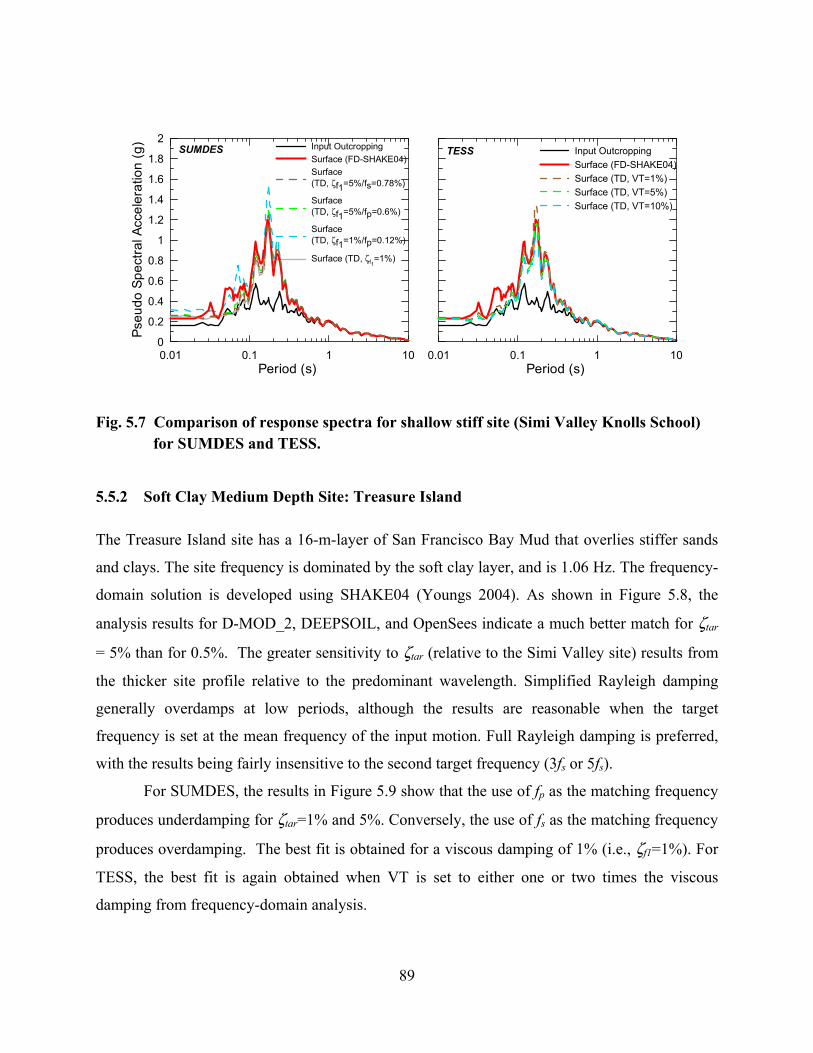
89

0.01 0.1 1 10Period (s)

0

0.2

0.4

0.6

0.8

1

1.2

1.4

1.6

1.8

2Ps

eudo

Spe

ctra

l Acc

eler

atio

n (g

) Input OutcroppingSurface (FD-SHAKE04)Surface (TD, ζf1=5%/fs=0.78%)

Surface (TD, ζf1=5%/fp=0.6%)

Surface(TD, ζf1=1%/fp=0.12%)

Surface (TD, ζf1=1%)

0.01 0.1 1 10Period (s)

Input OutcroppingSurface (FD-SHAKE04)Surface (TD, VT=1%)Surface (TD, VT=5%)Surface (TD, VT=10%)

SUMDES TESS

Fig. 5.7 Comparison of response spectra for shallow stiff site (Simi Valley Knolls School) for SUMDES and TESS.

5.5.2 Soft Clay Medium Depth Site: Treasure Island

The Treasure Island site has a 16-m-layer of San Francisco Bay Mud that overlies stiffer sands

and clays. The site frequency is dominated by the soft clay layer, and is 1.06 Hz. The frequency-

domain solution is developed using SHAKE04 (Youngs 2004). As shown in Figure 5.8, the

analysis results for D-MOD_2, DEEPSOIL, and OpenSees indicate a much better match for ζtar

= 5% than for 0.5%. The greater sensitivity to ζtar (relative to the Simi Valley site) results from

the thicker site profile relative to the predominant wavelength. Simplified Rayleigh damping

generally overdamps at low periods, although the results are reasonable when the target

frequency is set at the mean frequency of the input motion. Full Rayleigh damping is preferred,

with the results being fairly insensitive to the second target frequency (3fs or 5fs).

For SUMDES, the results in Figure 5.9 show that the use of fp as the matching frequency

produces underdamping for ζtar=1% and 5%. Conversely, the use of fs as the matching frequency

produces overdamping. The best fit is obtained for a viscous damping of 1% (i.e., ζf1=1%). For

TESS, the best fit is again obtained when VT is set to either one or two times the viscous

damping from frequency-domain analysis.

90

00.20.40.60.8

11.21.41.61.8

22.2

Pseu

do S

pect

ral A

ccel

erat

ion

(g)



00.20.40.60.8

11.21.41.61.8

22.2

Pseu

do S

pect

ral A

ccel

erat

ion

(g)

0.01 0.1 1 10Period (s)

00.20.40.60.8

11.21.41.61.8

22.2

Pseu

do S

pect

ral A

ccel

erat

ion

(g)

Target viscous damping ratio usedin D-MOD_2 is 0.5%

0.01 0.1 1 10Period (s)





Fig. 5.8 Comparison of response spectra for mid-period site with large impedance contrast

(Treasure Island) for D-MOD_2, DEEPSOIL, and OPENSEES.

91

0.01 0.1 1 10Period (s)

00.20.40.60.8

11.21.41.61.8

22.22.42.62.8

3

Pseu

do S

pect

ral A

ccel

erat

ion

(g) Input Outcropping

Surface (FD-SHAKE04)Surface (TD, ζf1=5%/fs=4.72%)




0.01 0.1 1 10Period (s)


SUMDES TESS

Fig. 5.9 Comparison of response spectra for mid-period site with large impedance contrast

(Treasure Island) for SUMDES and TESS.

5.5.3 Deep Stiff Site: La Cienega

The La Cienega site consists of bedded sands, silts, and clays that gradually increase in stiffness

with depth. Only the upper 305 m of the profile is modeled, which has a site frequency of 0.45

Hz, although the true first-mode site frequency is much lower because crystalline bedrock occurs

at great depth.

The frequency-domain solution is developed using SHAKE04 (Youngs 2004). As shown

in Figure 5.10, analysis results for D-MOD_2, DEEPSOIL, and OpenSees show high sensitivity

to ζtar (with 5% providing the better match). Simplified Rayleigh damping is most effective

when the target frequency is set to the mean frequency of the input motion (fm), and overdamps

the computed response otherwise. Full Rayleigh damping generally provides an improved fit,

with a slight preference towards the second frequency being 5fs.

For SUMDES, the results in Figure 5.11 show similar trends to those for Treasure Island:

the use of fp at the matching frequency produces underdamping whereas the use of fs produces

overdamping. The best fit is again obtained for a viscous damping of ζf1=1%. For TESS the best

fit is again obtained when VT is set to either one or two times the viscous damping from the

frequency-domain analysis.

92

0

0.2

0.4

0.6

0.8

1

1.2

1.4Ps

eudo

Spe

ctra

l Acc

eler

atio

n (g

)



0

0.2

0.4

0.6

0.8

1

1.2

1.4

Pseu

do S

pect

ral A

ccel

erat

ion

(g)

0.01 0.1 1 10Period (s)

0

0.2

0.4

0.6

0.8

1

1.2

1.4

Pseu

do S

pect

ral A

ccel

erat

ion

(g)

Target viscous damping ratio usedin D-MOD_2 is 0.5%

0.01 0.1 1 10Period (s)





Fig. 5.10 Comparison of response spectra for long-period site (La Cienega) for D-MOD_2,

DEEPSOIL, and OPENSEES.

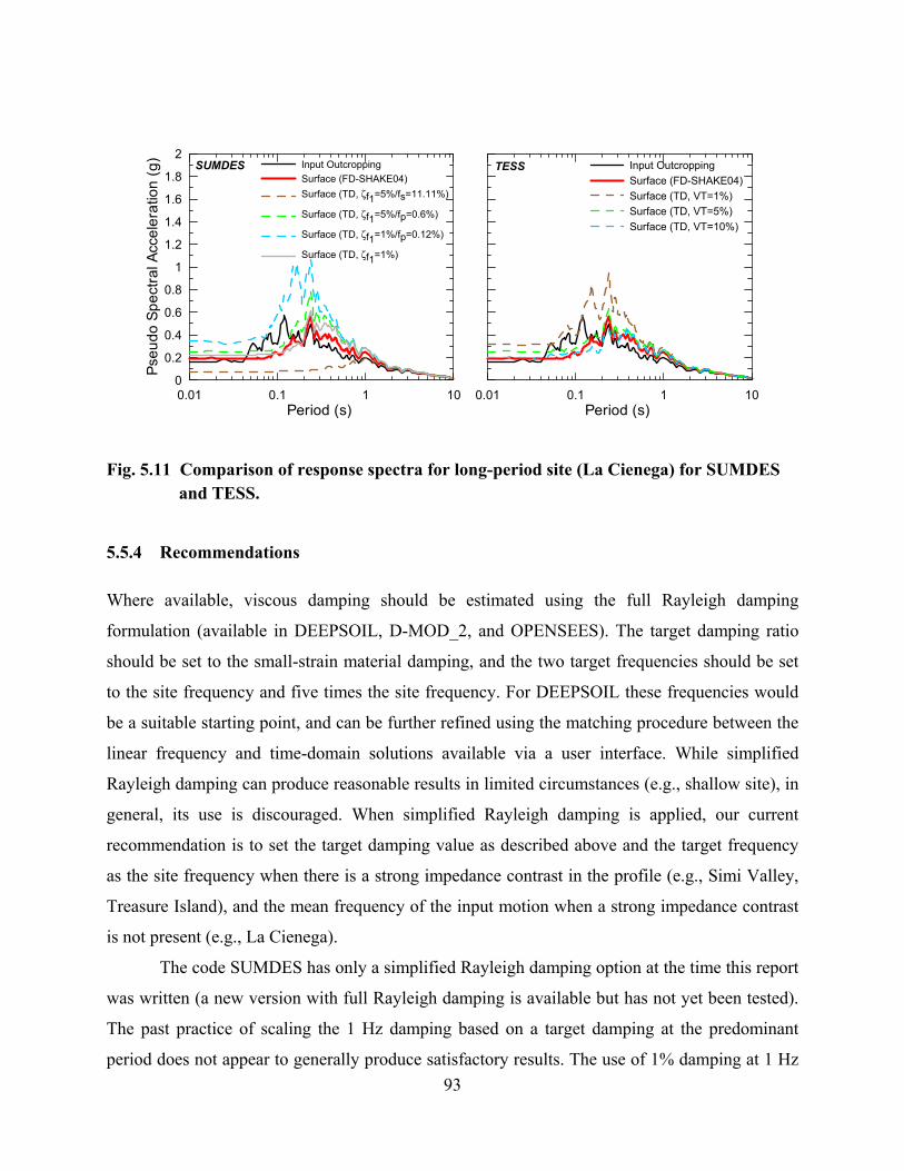
93

0.01 0.1 1 10Period (s)

0

0.2

0.4

0.6

0.8

1

1.2

1.4

1.6

1.8

2Ps

eudo

Spe

ctra

l Acc

eler

atio

n (g

) Input OutcroppingSurface (FD-SHAKE04)Surface (TD, ζf1=5%/fs=11.11%)




0.01 0.1 1 10Period (s)


SUMDES TESS

Fig. 5.11 Comparison of response spectra for long-period site (La Cienega) for SUMDES and TESS.

5.5.4 Recommendations

Where available, viscous damping should be estimated using the full Rayleigh damping

formulation (available in DEEPSOIL, D-MOD_2, and OPENSEES). The target damping ratio

should be set to the small-strain material damping, and the two target frequencies should be set

to the site frequency and five times the site frequency. For DEEPSOIL these frequencies would

be a suitable starting point, and can be further refined using the matching procedure between the

linear frequency and time-domain solutions available via a user interface. While simplified

Rayleigh damping can produce reasonable results in limited circumstances (e.g., shallow site), in

general, its use is discouraged. When simplified Rayleigh damping is applied, our current

recommendation is to set the target damping value as described above and the target frequency

as the site frequency when there is a strong impedance contrast in the profile (e.g., Simi Valley,

Treasure Island), and the mean frequency of the input motion when a strong impedance contrast

is not present (e.g., La Cienega).

The code SUMDES has only a simplified Rayleigh damping option at the time this report

was written (a new version with full Rayleigh damping is available but has not yet been tested).

The past practice of scaling the 1 Hz damping based on a target damping at the predominant

period does not appear to generally produce satisfactory results. The use of 1% damping at 1 Hz

94

appears to provide improved performance, and is simpler to apply. For TESS, a good match to

the SHAKE04 results is obtained when the parameter VT is set equal to the desired damping

ratio but the results obtained are not particularly sensitive to VT across the range of the desired

damping ratio to two times that figure.

5.6 CONCLUSIONS

Frequency-domain equivalent-linear methods of performing site response analysis remain

significantly more popular in practice than time-domain nonlinear methods (Kramer and Paulsen

2004). One reason this practice persists is that parameter selection for frequency-domain analysis

is relatively straightforward, requiring only mass density, shear wave velocity, and nonlinear

modulus reduction and damping versus shear strain curves. As a profession, we are well

equipped to provide estimates of these quantities on a site-specific basis at reasonable cost.

In contrast, time-domain nonlinear methods of analysis require the use of parameters that

are less familiar to most engineers and/or relatively difficult to obtain (details below). Three

major hurdles must be overcome before nonlinear analysis methods can be more widely adopted

in practice. The first is clarification of the manner in which input motions should be specified.

The second is the development of simple, practical guidelines for the specification of parameters

that provide element damping at small strains. In this chapter, these first two issues are addressed

by comparing the results of linear time-domain analyses to exact solutions from the frequency-

domain analyses for elastic conditions. The third issue, which would be investigated in

subsequent chapters, is the development of practical and well-validated guidelines for estimating

parameters that describe the backbone curve of soil and the unload/reload behavior given

conventionally available data from a site investigation program (shear wave velocity and soil

index properties).

The major finding on the input motion issue is that outcropping control motions should

be used as-recorded with an elastic base. Motions recorded at depth should also be used as-

recorded but with a rigid base. In both cases, the motions are specified at the base of the site

profile. For within motions, the depth at which the recording was made should match the depth

of the profile base.

With respect to the viscous damping issue, when the option of using more than one target

frequency is available (such as the full Rayleigh damping formulation), it should be applied in

95

lieu of simplified Rayleigh damping because significant bias at high frequencies can occur with

the latter. Target damping ratios should be set to the small-strain material damping, and the two

target frequencies in a full Rayleigh damping formulation should be set to the site frequency and

five times the site frequency. For DEEPSOIL these frequencies would be a suitable starting

point, and can be further refined using the matching procedure between linear frequency and

time-domain solutions available via a user interface. Specialized recommendations were

developed for SUMDES and its simplified Rayleigh damping formulation. Recommendations

are also developed for relating parameter VT to small-strain damping in the LSDS utilized in

TESS. Whenever possible, it is recommended that a check be made that linear time-domain and

linear frequency-domain solution provide similar results.

6 Turkey Flat Blind Prediction

In this chapter, ground response analysis codes (equivalent-linear and nonlinear codes described

in Chapter 2) are exercised for the blind prediction of motions recorded at the Turkey Flat

vertical array. The chapter begins with a review of previous studies performed at the Turkey Flat

site. The site conditions and the geotechnical model used for analysis are then described.

Nonlinear code usage protocols that are based on material originally presented in Chapters 4 and

5 are then summarized. The sensitivity of the predictions to model variability and to variability in

the site velocity profile and nonlinear soil properties is documented. The blind predictions are

compared to data and reasons for the misfit are investigated. Data from multiple earthquakes

recorded between 2003 and 2004 at the Turkey Flat site are used to compile site amplification

factors at specific frequencies, which are compared with model predictions to investigate event-

to-event variability in the misfit. Lastly, code performance at higher input shaking levels is

studied, from which the variability between equivalent-linear and nonlinear results are evaluated.

6.1 INTRODUCTION

In 1987, the California Geological Survey (CGS) and its strong-motion instrumentation program

established a seismic site effects test area at Turkey Flat, which is a shallow valley site. The

Turkey Flat site is located near Parkfield in the central California Coastal Range about 5 km east

of the Parkfield segment of the San Andreas fault. The objective of the Turkey Flat experiment

was to systematically test and compare the reliability of contemporary methods of estimating the

influence of site conditions on ground motions during earthquakes (Tucker and Real 1986). An

extensive site characterization program, including field and laboratory geotechnical

measurements, was conducted by numerous industrial, academic, and government organizations

to develop a standard geotechnical model of the test area, which would provide the input

parameters necessary for the site response estimation (Real 1988). Strong- and weak-motion

98

instruments were installed and have recorded numerous earthquakes with weak and strong

ground motions since 1987.

Weak motions recorded in the early years of operation of the Turkey Flat array were used

to develop empirical transfer functions for the site (Cramer 1995) and to conduct a weak-motion

blind prediction exercise (Real and Cramer 1989; Cramer and Real 1992). The chosen weak

motion for the prediction exercise was an Mw 2 event located about 32 km north of the test site

that was recorded on 27 April 1988. The blind prediction had a first stage in which participants

were given the outcrop motion at a nearby bedrock site in the first phase and a downhole motion

below the middle of the valley in the second phase. Participants were required to predict the site

response of the valley and uncertainties of their results using the standard geotechnical model.

They were also encouraged to submit predictions based on their own preferred geotechnical

model. The major results of the weak-motion blind prediction exercise were that (1) most

predictions tended to cluster together regardless of the geotechnical and site response model used

(preferred and standard velocity profiles were generally fairly similar) and (2) the shape and

frequency of resonant peaks predicted by models were similar to observation, but the amplitude

of site amplification was significantly overestimated for frequencies higher than the site

frequency.

Cramer and Real (1992) concluded that variability in the geotechnical model associated

with uncertainty in stiffness and damping characteristics more significantly impacted the

predicted motions than variability between different methods of analysis utilizing relatively

consistent velocity profiles (i.e., from preferred versus standard geotechnical models). To further

investigate the prediction bias noted in the weak-motion blind prediction exercise, Field and

Jacob (1993) performed Monte-Carlo simulations to investigate the sensitivity of site response

predictions to variability in the seismic velocity profile (including variability in layer velocities

and layer thickness) and variability in damping, using the standard geotechnical model as a

baseline. Factors that significantly contributed to the scatter of the predicted site amplification

included the first-layer shear wave velocity and thickness, as well as the profile damping (one

value was used for the entire soil layer). The variability in the properties of deeper layers did not

significantly impact the results. Cramer (1995) performed sensitivity studies similar to those of

Field and Jacob (1993), and found that the fit of the predicted response to observation was

optimized by increasing (relative to the standard geotechnical model) shear wave velocities

99

throughout the site profile by 5% and increasing the damping from the average laboratory-

reported value of 1.5%–7%.

The strongest motions recorded at the Turkey Flat site are from the Mw 6.0 Parkfield

earthquake on 28 September 2004, which occurred on the Parkfield segment of the San Andreas

fault (Rymer et al. 2006). The strong motions from this event were used in a second blind

prediction exercise for the Turkey Flat site (Real and Shakal 2005). The strong-motion blind test

procedure was similar to that for the weak-motion blind test, with the additional consideration

that nonlinear geotechnical properties (such as modulus reduction and damping curves) were a

significant component of these analyses. The emphasis of this chapter is on Phase II of the blind

prediction exercise, which focuses on ground response at the valley center conditioned on the

within (rock) motion.

6.2 TURKEY FLAT ARRAY

Turkey Flat is a shallow stiff-soil alluvial valley near Parkfield, California. The valley is

instrumented with surface and downhole sensors as indicated in the vertical schematic section

shown in Figure 6.1. One of the vertical arrays is outside the valley (location is referred to as

rock south) in upper Cretaceous and Tertiary sedimentary sandstone bedrock materials and

consists of two instruments referred to as R1 (surface) and D1 (downhole). The second vertical

array is at the valley center and consists of three instruments: V1 (surface) and D2–D3

(downhole). As shown in Figure 6.1, additional surface instruments are at the north end of the

valley (valley north, V2) and on rock north of the valley (rock north, R2).

At the time of the original array installation in 1987, each sensor location consisted of

digital three-component forced-balance accelerometers and three-component velocity sensors

(Real et al. 2006). In 2001, the data acquisition system was upgraded with 12-bit solid-state

digital recorders, which recorded all of the data utilized in this chapter.

The blind predictions reported in this chapter were part of a larger blind prediction

exercise organized by the California Strong Motion Instrumentation Program in 2005 (Real and

Shakal 2005) with multiple U.S. and international participants. The prediction exercise consisted

of two phases, both using data from the 2004 Parkfield earthquake. In the first phase, rock-

surface motion R1 was released, and the motions were predicted at D1 and D3 (rock downhole)

and D2 and V1 (soil motions). In the second phase, rock downhole motion D3 was provided, and

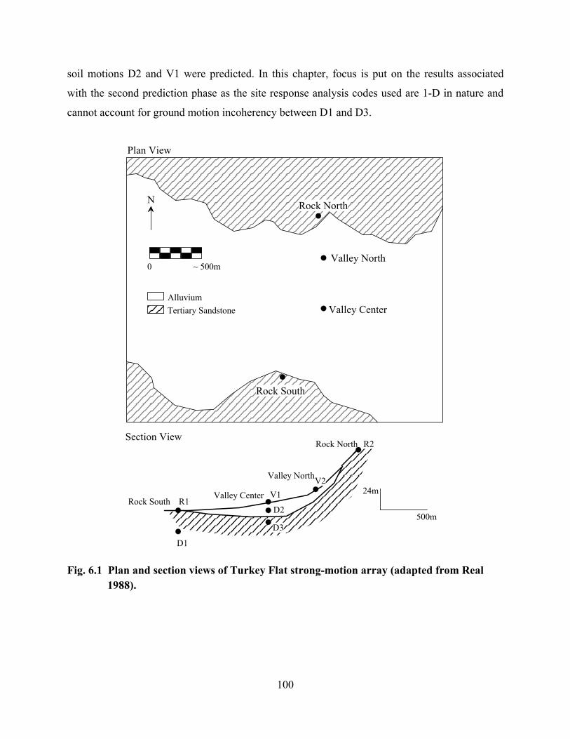
100

soil motions D2 and V1 were predicted. In this chapter, focus is put on the results associated

with the second prediction phase as the site response analysis codes used are 1-D in nature and

cannot account for ground motion incoherency between D1 and D3.

Rock SouthValley Center

Valley North

Rock North

R1

D1

D3

R2

V2V1

D2500m

24m

Plan View

Section View

N Rock North

Valley North

Valley Center

Rock South

0 ~ 500m

Alluvium Tertiary Sandstone

Fig. 6.1 Plan and section views of Turkey Flat strong-motion array (adapted from Real 1988).

101

6.3 SITE PROPERTIES AND BASELINE GEOTECHNICAL MODEL

According to Real (1988), boreholes were drilled at Turkey Flat in 1986–1987 at the locations of

the two vertical arrays to investigate geotechnical conditions and to enable installation of

downhole sensors. The maximum depths of exploration were 25 m and 40 m for rock south and

valley center, respectively. At the rock south array, surficial materials consist of weathered

grayish-brown sandstone that transition to a lower degree of weathering at approximately 14 m

(as indicated, e.g., by color change to bluish gray). At the valley center array, the soil profile

consists of dark-brown silty clay near the surface (about 1.8–4.6 m), which is underlain by

clayey sand to a depth of about 20 m. Underlying the soil materials is a sandstone bedrock

profile similar to that at rock south. Estimated values of material density at the valley center site

are shown in Table 6.1.

Table 6.1 Estimated values of material density at valley center site.

Unit Weight (kN/m3)Soft surface soil 0 - 1.8 15.7Deep stiff soil and weathered rock 1.8 - 22.9 17.6Bedrock below weathering zone 21.5

Depth (m)

> 22.9

Shear wave velocity (Vs) measurements were made in boreholes at the two vertical arrays using

downhole, crosshole, and suspension logging methods performed by numerous groups including

LeRoy Crandall and Associates, Hardin Lawson Associates, QEST Consultants, OYO

Corporation, Kajima Corporation, the California Division of Mines and Geology, and

Woodward-Clyde Consultants. Figure 6.2 shows data for the valley center site (V1-D3) along

with a weighted mean and mean ± one standard deviation profiles. Equal weights were given to

all velocity profiles except for the OYO suspension-logger profile, which was given double

weight below 4.5 m depth (because of relatively high signal/noise ratios at depth with OYO data

due to a constant spacing between source and receiver; Nigbor and Imai 1994). It is noteworthy

that the mean Vs profile in Figure 6.2 implies an upward wave travel time of 0.045 sec, which

compares favorably to travel times derived from analysis of V1-D3 seismographs (using cross-

correlations functions) of 0.05 ± 0.01 sec.

102

Also shown in Figure 6.2 is a smoothed velocity profile developed by K. Stokoe (2006,

pers. comm.).that includes a transition zone from 1–3.6 m depth between a soft surface layer and

relatively stiff soils at depth and a second transition zone reflecting apparent bedrock weathering

from 20–26 m depth. This smoothed profile implies a median travel time of 0.042 sec, and hence

is also consistent with seismograph data. A similar bedrock transition zone thickness was

observed at the rock site south vertical array (R1-D3) near the ground surface.

Finally, we show in Figure 6.2 a profile developed following the blind prediction exercise

from a spectral analysis of surface waves (SASW) tested by R. Kayen (personal comm. 2007).

The line of sensors used for SASW testing was positioned adjacent to the valley center recording

station. This velocity profile has a similar shape to the earlier profiles but has lower shear-wave

velocities from 2–33 m. The shear-wave travel time implied by this model is 0.056 sec, which is

in the plausible range of observed values from seismograms (0.05 ± 0.01 sec).

During the 1986–1987 field work, soil samples were retrieved from boreholes at the mid

valley location using Pitcher barrel (pushed/carved) and Crandall (driven-tube) samplers. Cyclic

laboratory testing was performed on specimens carved from those samples to measure nonlinear

relationships between shear stress and shear strain and between hysteretic damping ratio and

shear strain. The former are expressed in normalized form as modulus-reduction curves (G/Gmax

curves), the latter as damping ratio versus strain curves (β curves). The results obtained using

resonant column and cyclic triaxial testing are plotted on the left-hand side of Figure 6.3.

Regression model-based predictions of G/Gmax and β curves from Darendeli (2001) (which

account for soil plasticity, overconsolidation ratio, and overburden pressure) computed for

different depths are shown on the right-hand side of Figure 6.3. Values for all of the input

parameters needed to exercise the Darendeli model are given in Figure 6.3. The material-specific

G/Gmax curves and Darendeli model predictions generally compare favorably. There are

differences in the damping, with the Darendeli damping predictions generally being lower than

the measured values. It is possible that the laboratory data, which date from 1986–1987, have an

overprediction bias (this is commonly the case with data from that time period). Accordingly, the

Darendeli curves are taken as the preferred model for the analyses described below.

103

0 500 1000 1500Vs (m/sec) at Central Valley

40

35

30

25

20

15

10

5

0D

epth

(m)

DataMeanMean + SigmaSmoothed profile (Stokoe, 2006, pers. comm.)SASW (Kayen, 2007, pers. comm.)

Darendeli Curve (refer to Fig. 6.3)

C1

C2C3

C4

C5

C6

C7

C8

C9

C10

Silty Clay

Silty Clay / Clayey Sand

Clayey Sand

Sandstone Fig. 6.2 Shear wave velocity profiles at mid-valley site (V1- D3 array). Data from Real,

(1988).

104

0.0001 0.001 0.01 0.1 10

0.2

0.4

0.6

0.8

1

G/G

max

CTX (z=7.6m; σ3=287ksf))CTX (z=7.6m; σ3=287ksf)CTX (z=12.2m; σ3=115kPa)CTX (z=12.2m; σ3=230kPa)RC (z=2.1m)RC (z=18.3m)

0.0001 0.001 0.01 0.1 1Cyclic Shear Strain (%)

0

5

10

15

20

25

30

Dam

ping

(%)

0.0001 0.001 0.01 0.1 1 100

0.2

0.4

0.6

0.8

1

G/G

max


0

5

10

15

20

25

30

Dam

ping

(%)

z=21.3 m (σ'v = 370 kPa)

z=0.9 m (σ'v = 14 kPa)

Intermediate depths:2.1, 4.0, 6.1, 7.6, 9.1, 12.2, 15.2, and 18.3 m

PI=0OCR=1.0N=2.4 cyclesf=2.8 Hz

Fig. 6.3 Modulus reduction and damping curves based on material-specific testing (left

side) and Darendeli (2001) model predictions (right side), mid-valley location. Data from Real (1988).

6.4 NONLINEAR SEISMIC GROUND RESPONSE ANALYSIS CODES

Six different ground response analysis codes were utilized: SHAKE04 (Youngs 2004), which is

a modified version of SHAKE91 (Idriss and Sun 1992); D-MOD_2 (Matasovic 2006);

DEEPSOIL (Hashash and Park 2001, 2002; Park and Hashash 2004); TESS (Pyke 2000);

OpenSees (Ragheb 1994; Parra 1996; Yang 2000; McKenna and Fenves 2001); and SUMDES

(Li et al. 1992). The total stress analysis option is used for all nonlinear codes considered.

6.5 CODE USAGE PROTOCOLS

The code usage protocols relate principally to three issues: (1) specification of input motion; (2)

specification of viscous damping model and parameters; and (3) specification of parameters

describing the nonlinear backbone curve and hysteretic damping behavior given a target set of

G/Gmax curves and β curves. It is possible to address the first two issues purely through the

comparison of simulation results from the nonlinear (time-stepping) codes to known theoretical

105

solutions for linear conditions. As presented in Chapter 5, the results of this work support the

following protocols, which were applied for the Turkey Flat analyses:

1. The recorded “within“ motions (D3) are taken as the input motion without modification,

and are used with a rigid base. Although not applied for Turkey Flat, we note for

completeness that an outcropping motion to be used as input would also be applied

without modification but would be specified in the nonlinear codes with a compliant

base.

2. For codes DEEPSOIL, D-MOD_2, and OpenSees, viscous damping is specified using

full Rayleigh damping, with the target frequencies set to the first-mode site frequency (fs)

and 3×fs. The general protocol that is followed here is to use full Rayleigh damping (two

matching frequencies) in lieu of simplified Rayleigh damping (one matching frequency)

when available. The level of damping that is specified is the small-strain hysteretic

damping, referred to as Dmin. The frequencies at which matching of the target damping

value are enforced are the site frequency above the elevation at which the input motion is

specified (fs) and a higher frequency selected to optimize the match of linear frequency

and time-domain analyses (Hashash and Park 2002). In the case of the Turkey Flat site,

this optimal match occurred for a second matching frequency of 3×f. For TESS,

parameter VT is taken as equal to Dmin. For SUMDES, the target damping ratio is set to

be 1% as demonstrated in Chapter 5.

The remaining parameters required to apply the nonlinear codes describe the nonlinear

backbone curve and hysteretic damping behavior. There are two principal issues here. The first is

the selection of target soil properties to be replicated as accurately as possible in the codes’

nonlinear models. The second issue is the manner in which input parameters describing the

codes’ nonlinear models are selected given a set of target material properties. Regarding the

former issue, the required soil properties are the small-strain shear wave velocity (Vs) profile,

density, and modulus reduction and damping curves (G/Gmax and β). We define our baseline

geotechnical model as the mean Vs profile in Figure 6.2, the unit weight values in Table 6.1, and

Darendeli model-based G/Gmax and β curves in Figure 6.3. the variability in the most important

of these parameters (i.e., the Vs profile and G/Gmax and β curves) is also considered, as described

further in the next paragraph.

106

The input parameters in nonlinear codes that describe nonlinear backbone curves and

hysteretic damping behavior generally consist of Gmax, a pseudo-reference strain parameter (γr)

defined as the value of shear strain at which G/Gmax=0.5, and additional curve-fitting parameters.

The specification of Gmax is trivial. The specification of γr and additional fitting parameters are

relatively subjective because it is not possible to simultaneously match (1) the target G/Gmax

curves to the G/Gmax behavior of the backbone curve and (2) the target β curves to the hysteretic

damping that results from the application of extended Masing rules (or similar Cundall-Pyke

rules) for unload-reload behavior to the backbone curve. For the present analysis, we selected γr

and additional curve-fitting parameters to match the target G/Gmax curves. Although this

generally would produce misfit of the target β curves as shown in Figure 6.4, the misfit is

negligibly small over the strain range of interest from the recorded ground motions (as noted in

the figure).

0.0001 0.001 0.01 0.1 1Cyclic Shear Strain (%)

0

10

20

30

40

50

60

Dam

ping

(%)

Masing + viscousTarget (depth = 0.9-1.8 m)

Strain range

Fig. 6.4 Target and modeled damping curves for 0.91–1.82 m (depth range at which

largest strains occur in soil profile).

6.6 RESULTS OF SIMULATION AND COMPARISONS TO DATA

6.6.1 Blind Prediction Results Using Baseline Model

We performed ground response analyses to estimate soil motions V1 and D2 using recording D3

as the input motion. Analyses were performed using the six different codes described above.

Each code was exercised for the same baseline site condition.

107

Figures 6.5 and 6.6 present the results of the simulations and how they compare to the

recorded data. The simulation results in Figures 6.5 and 6.6 are truly “blind,” meaning they were

established before the strong motion data were released [the simulation results were published in

the proceedings of a conference from August 30–September 1, 2006 (Kwok et al. 2006), which

was prior to a Turkey Flat workshop at which all the data were released on September 21, 2006].

Figure 6.5 compares the recorded acceleration histories to the simulations from DEEPSOIL. It

can be seen that shear waves dominate the signal and that the predicted waveforms are similar to

observation except for amplitudes that are slightly too low. The results in Figure 6.6 are

presented in terms of 5% damped pseudo-acceleration response spectra (Sa) and Sa residuals (R)

defined as:

( ) ( )preadataa TSTSTR )(ln)(ln)( −= (6.1)

where ( )dataa TS )( indicates the spectra of recordings and ( )prea TS )( indicates the spectra of

model predictions. The results are shown for two horizontal directions at the surface (V1) and at

10 m depth (D2).

The elastic fundamental period (Ts = 1/fs) of the Turkey Flat site is 0.18 sec. Given the

modulus reduction relationships for the site soils, the elongated site period is approximately

0.19–0.20 sec. As shown in Figure 6.6a–d, at periods well beyond the elongated site period, the

simulation results match the surface recordings well and are very similar to each other, which is

expected because the computed site effect at such periods is negligible (nearly rigid body

motion). At shorter periods, the simulations generally underpredict the surface recorded motions

(especially in the EW direction) and the simulation results demonstrate significant code-to-code

variability. An exception to this underprediction trend occurs in the NS direction near the site

period, where the motions are overpredicted. As shown in Figure 6.5e–h, the positive residuals

that are present in the surface recordings are significantly reduced for the downhole soil

recording, which suggests that the upper part of the profile contributes significantly to the

underprediction misfit. However, the overprediction in the NS direction near the site period is

not reduced, indicating that the source of this misfit is not only related to surficial soil conditions.

Because the codes are being run for the same geotechnical model, the aforementioned

code-to-code variability arises from issues such as the manner in which the backbone curve is

parameterized and the viscous damping is specified. For example, the DEEPSOIL and D-

MOD_2 results are similar to each other because of the similarity of these models. The

108

SHAKE04 residuals are lower. The relatively high residuals from SUMDES result from

overdamping at high frequencies due to the use of the simplified Rayleigh damping formulation.

The TESS residuals are slightly higher because the damping generated by the Cundall-Pyke

hypothesis coupled with Pyke’s low-strain damping scheme is higher than what is generated by

Masing rules (see Chapter 5). The modulus reduction/damping curves and viscous damping

scheme used in OpenSees is similar to those used in DEEPSOIL and D-MOD_2; hence, the

differences in residuals (which are smaller in this case for OpenSees) is likely related both to

small differences in the constitutive models and to the soil being modeled as a finite element

continuum in OpenSees versus as lumped masses in DEEPSOIL and D-MOD_2. The code-to-

code variability shown in Figure 6.6 is found to be approximately log-normally distributed with a

standard deviation σm (subscript ‘m’ for model) ranging from zero beyond the site period to

approximately 0.15–0.20 (in natural log units) at shorter periods.

-0.2

0

0.2

Acc

(g) V1 - EW

-0.2

0

0.2

Acc

(g) D2 - EW

17 18 19 20 21 22Time (sec)

-0.2

0

0.2

Acc

(g) D3 - EW

V1 - NS

RecordedPredicted by DEEPSOIL

D2 - NS

17 18 19 20 21 22Time (sec)

D3 - NS

Fig. 6.5 Acceleration histories for data and simulation results from DEEPSOIL. Results shown for two horizontal directions and two elevations (V1, ground surface; D2, 10-m depth. Recorded input motions at elevation D3 also shown.

109

0.0

0.4

0.8

1.2

Sa (

g)

Surface (V1) Downhole rock (D3)

-0.8

-0.4

0.0

0.4

0.8

1.2

Res

idua

l, R

(ln

units

)

DEEPSOILD-MOD_2OpenSeesSUMDESTESSSHAKE2004

(a) V1-EW

0.0

0.4

0.8

1.2

Sa (

g)

Downhole soil (D2)Downhole rock (D3)

0.01 0.1 1Period (sec)

-0.8

-0.4

0.0

0.4

0.8

1.2

Res

idua

l, R

(ln

units

)

(e) D2-EW

(b) V1-NS

(c) V1-EW (d) V1-NS

(g) D2-EW


(f) D2-NS

(h) D2-NS

Fig. 6.6 Acceleration response spectra for data and simulation results compared through

direct spectral ordinates and prediction residuals. Results shown for two horizontal directions and two elevations (V1 = ground surface; D2 = 10 m depth). Results shown to a maximum period of 1/(1.25×fHP), where fHP = high-pass corner frequency.

110

6.7 UNCERTAINTY IN PREDICTION RESULTS FROM VARIABILITY IN MATERIAL PROPERTIES

As shown in Figures 6.2 and 6.3, there is significant uncertainty in soil properties at the Turkey

Flat site. The impact of that uncertainty on the simulation results is of interest both from the

standpoint of understanding whether “observations” lie within an expected band of prediction

results and understanding the most important sources of variability in the predictions. Two

sources of material property variability are considered—variability in Vs as represented by the

scatter of the field measurements and variability in modulus reduction and damping relationships

as established in the literature.

The impact of variability in the velocity profile was investigated by performing analyses

with the baseline geotechnical model, but with velocities varied to reflect mean ± 3 standard

deviation profiles. The corresponding response variability was assessed using three runs (for the

three different velocity profiles) with the DEEPSOIL code. A weighted variance is calculated

from the three results, giving a weight of 2/3 to the mean velocity profile and 1/6 to the mean ±

3 standard deviation profiles. The standard deviation of the ground motions due to the

variability in velocity (denoted σv) is then taken as the square root of the weighted variance. This

is consistent with a first-order second- moment method for estimating response variability given

input parameter variability (Melchers 1999; Baker and Cornell 2003).

The target modulus reduction and damping curves used in the predictions are from an

empirical model (Darendeli 2001). The Darendeli model includes estimates of standard deviation

on the modulus reduction and damping curves. These standard deviation estimates are based on

the scatter of the laboratory data used to develop the regression model. We utilize these standard

deviation estimates to evaluate the uncertainty on modulus reduction behavior. At G/Gmax = 0.5,

the uncertainty on the modulus reduction curves corresponds to a coefficient of variation of

approximately 0.2. Since in the nonlinear codes the shape of the backbone curve also affects the

damping, uncertainty in damping curves is not considered separately (i.e., variability in damping

was assumed to be perfectly correlated to variability in modulus reduction). So the impact of

material curve variability was evaluated by performing analyses with the baseline geotechnical

model and modulus reduction curves varied to reflect mean ± 3 standard deviation. The

111

standard deviation of the ground motions associated with material curve variability is termed σG

and is evaluated in a manner similar to what was described previously for σv.

The values of the standard deviation terms σm, σv, and σG are summarized in Figure 6.7

for the geometric mean of the spectral accelerations at location V1 in the two horizontal

directions. Also shown in Figure 6.7 is the total standard deviation (σ) calculated assuming that

the three sources of variability are uncorrelated:

2 2 2m v Gσ σ σ σ= + + (6.2)

The most significant source of dispersion below the site period (Ts = 0.18 sec) is velocity

variability. The dominant effect of velocity variability across a relatively broad range of periods,

including the elastic and elongated site period, is consistent with the previous simulation results

of Field and Jacob (1993).


0

0.5

1

Estim

ated

sta

ndar

d de

viat

ion

in p

redi

ctio

n (ln

uni

t)

Overall, σVelocity, σv

Model, σm

Material Curve, σG

Ts = 0.18 sec

Fig. 6.7 Standard deviation terms associated with geometric mean acceleration response spectral ordinates for location V1. Ts denotes elastic site period.

To evaluate whether model and material property variability could explain the

underprediction bias reported in Figure 6.6 for surface recordings (V1), we add and subtract the

total standard deviation (black line in Fig. 6.7) to the median of the residuals for the baseline

geotechnical model (i.e., the median of the residuals shown in Fig. 6.6). As shown in Figure 6.8,

the results indicate that at a mean ± one standard deviation level, the prediction residuals include

an unbiased condition (zero residual) for most periods smaller than the site period. This result

112

indicates that 1D ground response analysis with the material data available at the time of the

blind prediction exercise may be capable of explaining the observed site amplification.

Nonetheless, the best-estimate properties produce a clear bias for which we postulate two

explanations. One is that the analytical models contain inherent flaws in model formulation (e.g.,

the assumption of 1D wave propagation). The other possibility is that the measured or assumed

material properties are incorrect. This issue is explored further in the next section.


-1.5

-1.0

-0.5

0.0

0.5

1.0

1.5

Res

idua

l, R

(ln

units

)

Median + 1 std. dev.

(a) V1-EW


(b) V1-NS

Fig. 6.8 Median ± one standard deviation residuals using total standard deviation

estimate from Fig. 6.7.

6.8 INVESTIGATION OF POSSIBLE SOURCES OF BIAS

As noted in the previous section, the prediction bias reported in Figures 6.6 and 6.8 could result

from errors in the model formulation or errors in material properties. We consulted with a

number of collaborating experts in nonlinear ground response analysis (N. Matasovic, R. Pyke,

Y. Wang, Z. Yang 2006, pers. comm. 2006) asking them to independently investigate possible

reasons for the bias. Most investigated the potential for the bias to have resulted from

overestimation of damping in the models (hysteretic and viscous) and overestimation of shear

wave velocity (Vs) in the near-surface soils. In this section, we report representative results of

such sensitivity studies using the code DEEPSOIL are reported. Similar results were obtained by

the aforementioned code developers using each of their respective nonlinear codes.

Modifications of damping were found to significantly affect the prediction bias only at

very low periods (T < 0.07 sec). A typical result is shown in Figure 6.9, which shows

DEEPSOIL residuals with the baseline geotechnical model, the baseline model with lower

113

hysteretic damping (one standard deviation lower than the baseline damping), and lower viscous

damping (decreased from 0.7–1.9% to 0.5 % for all layers).

0.0

0.4

0.8

1.2

Sa (

g)



-0.8

-0.4

0.0

0.4

0.8

1.2

Res

idua

l, R

(ln

units

)

Baseline DampingReduced βReduced Viscous

(a)

(b)

Fig. 6.9 Geometric mean acceleration response spectra and prediction residuals for

DEEPSOIL simulation results obtained with alternative material curves and viscous damping formulation.

Two types of modifications to the Vs profile were considered by the code developers in

their attempts to reduce high-frequency residuals. The first involved smoothing the relatively

jagged baseline profile. This tended to further increase residuals because the smoothing process

would typically involve decreasing the thickness of the low velocity surface layer. For example,

the modification of residuals obtained using the smoothed profile from Figure 6.2 are shown in

Figure 6.10. Additional attempts to smooth the Vs profile without changing the thickness of the

surface layer resulted in effectively no change in residuals relative to the baseline result.

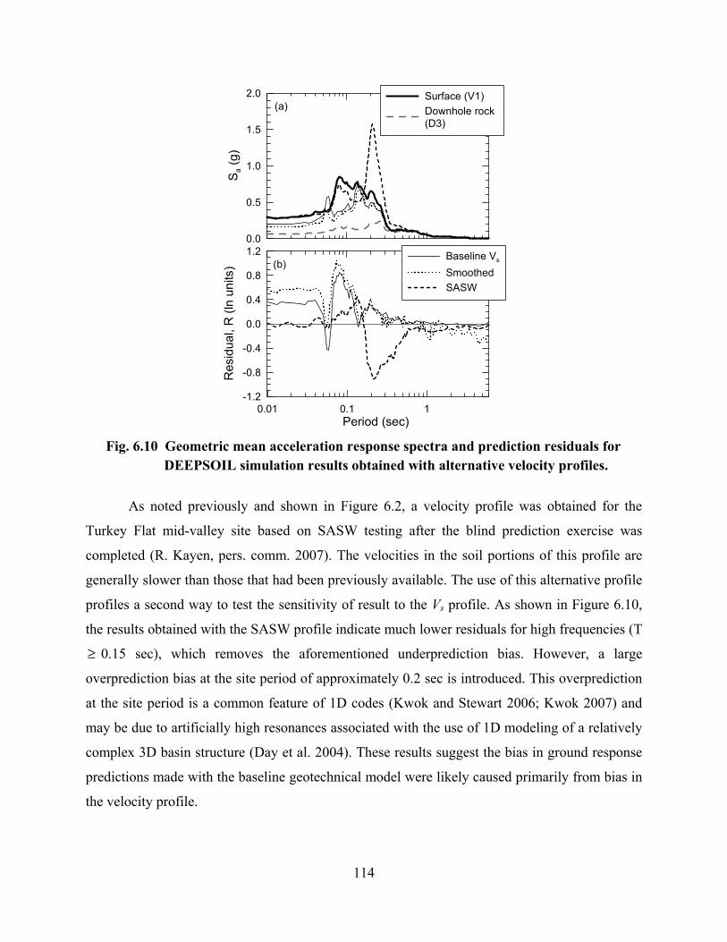
114

0.0

0.5

1.0

1.5

2.0

Sa (

g)



-1.2

-0.8

-0.4

0.0

0.4

0.8

1.2

Res

idua

l, R

(ln

units

)

Baseline Vs

SmoothedSASW

(a)

(b)

Fig. 6.10 Geometric mean acceleration response spectra and prediction residuals for

DEEPSOIL simulation results obtained with alternative velocity profiles.

As noted previously and shown in Figure 6.2, a velocity profile was obtained for the

Turkey Flat mid-valley site based on SASW testing after the blind prediction exercise was

completed (R. Kayen, pers. comm. 2007). The velocities in the soil portions of this profile are

generally slower than those that had been previously available. The use of this alternative profile

profiles a second way to test the sensitivity of result to the Vs profile. As shown in Figure 6.10,

the results obtained with the SASW profile indicate much lower residuals for high frequencies (T

≥ 0.15 sec), which removes the aforementioned underprediction bias. However, a large

overprediction bias at the site period of approximately 0.2 sec is introduced. This overprediction

at the site period is a common feature of 1D codes (Kwok and Stewart 2006; Kwok 2007) and

may be due to artificially high resonances associated with the use of 1D modeling of a relatively

complex 3D basin structure (Day et al. 2004). These results suggest the bias in ground response

predictions made with the baseline geotechnical model were likely caused primarily from bias in

the velocity profile.

115

6.9 EVENT-TO-EVENT VARIABILITY OF TURKEY FLAT SITE RESPONSE

As noted in the introduction, the first blind prediction exercise found the measured site response

at Turkey Flat from weak motions to be overpredicted using elastic wave propagation codes

(Cramer and Real 1992). Conversely, the strong motion site response from the 2004 Parkfield

earthquake is underpredicted. Although the codes used for the two prediction exercises are

different, it is nonetheless clear that there is some event-to-event variability in the ground

response analysis residuals. To investigate this more formally, we compile site amplification

factors from ground motions recorded at Turkey Flat from 2003–2004. The earthquake events

considered are summarized in Table 6.2.

Table 6.2 Earthquake events used to compile site amplification factors.

Hypocentral Site-source PGA at D3 PGA at V1 Depth (km) Distance (km) (Geo Mean, g) (Geo Mean, g)

San Simeon 2003 12 22 1115 6.5 35.71 121.10 4.7 70.4 0.019 0.034Parkfield Mainshock 2004 9 28 1015 6.0 35.81 120.37 7.9 8.2 0.067 0.292Parkfield Aftershock 1 2004 9 28 1019 4.2 35.86 120.41 9.2 5.9 0.030 0.127Parkfield Aftershock 2 2004 9 28 1022 4.0 35.84 120.39 5.6 5.9 0.011 0.071Parkfield Aftershock 3 2004 9 28 1033 3.7 35.82 120.36 6.9 7.0 0.006 0.025Parkfield Aftershock 4 2004 9 28 1035 3.6 35.95 120.49 10.2 14.7 0.002 0.007Parkfield Aftershock 5 2004 9 28 1223 3.1 35.83 120.38 6.5 6.4 0.003 0.016Parkfield Aftershock 6 2004 9 28 1231 4.0 35.84 120.39 9.3 5.9 0.007 0.037Parkfield Aftershock 7 2004 9 29 1010 5.0 35.95 120.50 11.5 15.5 0.016 0.036Parkfield Aftershock 8 2004 9 29 1012 3.8 35.95 120.49 10.2 14.7 0.002 0.006

Longitude (W)Event Year Month Day hhmm Magnitude Latitude (N)

Amplification factors (V1/D3) of geometric mean response spectral accelerations are

derived at specified periods using the baseline geotechnical model for all codes. To estimate

amplification factors for different amplitudes of input motions, the D3 Parkfield recording is

scaled down to various degrees. Sensitivity analyses performed using different D3 waveforms

indicate that the amplification factors are not particularly sensitive to the details of the

waveform, and hence the amplification factors derived using the Parkfield mainshock recording

are sufficiently representative for the present application.

In Figure 6.11, we plot the theoretical amplification factors as a function of base motion

peak acceleration (PGAr) for comparison to the observed site amplification factors from

recordings. As shown in Figure 6.11, the trend with PGAr is similar for the theoretical and

empirical results, but for most events the site amplification is underpredicted by the models. The

model-to-model variation is generally small relative to this misfit. Accordingly, the conclusions

116

reached above about bias are unlikely to be event-specific phenomena, but something more

germane to the modeling.

1

10

AF

(T =

0 s

ec)

1

10

AF

(T =

0.1

sec

)

0.001 0.01 0.1 1PHAr (g)

1

10

AF

(T =

0.2

sec

)

0.001 0.01 0.1 1PHAr (g)

1

10

AF

(T =

0.5

sec

)

RecordedSHAKE2004DEEPSOILD-MOD_2TESSOpenSees

Fig. 6.11 Theoretical and observed V1/D3 amplification factors at Turkey Flat site for

events listed in Table 6.2.

6.10 CODE PERFORMANCE AT HIGHER SHAKING LEVELS

In this section, the code-to-code variability of spectral shape for different levels of site

nonlinearity is investigated. Ground response analyses with the baseline geotechnical model are

performed with input motions (Parkfield mainshock recording at D3) scaled to higher shaking

levels. Spectral shapes of the calculated motions at the ground surface for both horizontal

directions are studied.

It can be observed from Figures 6.12 and 6.13 that the spectral shapes from equivalent-

linear and nonlinear models are similar when the input motion level is low. However, at high

shaking levels (above PHAr of 0.2 g which corresponds to scale factor above 4), the spectral

shapes from equivalent-linear and nonlinear analyses start to deviate from each other. At periods

below the site frequency, the spectral shapes from equivalent-linear analyses are flatter and have

117

less period-to-period fluctuations than those from nonlinear analyses. The spectral shapes

ordinates at the site period also tend to be larger for nonlinear models. Note also that at strong

shaking levels, the results of the various nonlinear codes differ significantly from each other.

0

1

2

3

4

5

6

7

Spe

ctra

l Sha

pe

DEEPSOILD-MOD_2OPENSEESSUMDESTESSSHAKE2004

0.01 0.1 1 10Period (s)

0

1

2

3

4

5

6

7

Spe

ctra

l Sha

pe

0.01 0.1 1 10Period (s)

Scale Factor = 1(PHAr = 0.07 g)




Fig. 6.12 Comparison of spectral shapes of predictions at different shaking levels for EW

component.

0

1

2

3

4

5

6

7

Spe

ctra

l Sha

pe

DEEPSOILD-MOD_2OPENSEESSUMDESTESSSHAKE2004

0.01 0.1 1 10Period (s)

0

1

2

3

4

5

6

7

Spec

tral S

hape

0.01 0.1 1 10Period (s)





Fig. 6.13 Comparison of spectral shapes of predictions at different shaking levels for NS

component.

118

6.11 CONCLUSIONS

The two blind prediction exercises performed using the Turkey Flat vertical array have provided

a valuable opportunity to investigate our ability to estimate seismic site response. This chapter

has focused on the second phase of the most recent blind prediction exercise and subsequent

analysis, involving relatively strong motion data from the 2004 Parkfield earthquake.

Using the original material properties provided as part of the prediction exercise, we find

that a series of equivalent-linear and nonlinear 1D ground response analysis codes generally

underestimate the observed site response over the period range where site response effects are

significant (i.e., below the elongated site period). It does not appear that the underestimation can

be explained by errors in the representation of damping in the models. We believe the observed

bias is a result of errors in the velocity profile. A recently obtained SASW profile (R. Kayen,

pers. comm. 2007) has slower velocities through much of the soil column, and results in a

significant reduction of residuals for periods lower than the site period. However, analyses with

this profile significantly overestimate the site response near the fundamental-mode site period.

The cause of this overestimation is the subject of ongoing research, but we suspect that it may be

a by-product of 1D modeling of relatively complex 3D site effects, as suggested by previous

simulation-based work (Day et al. 2004).

7 Verification of Nonlinear Codes against Vertical Array Data

7.1 INTRODUCTION

Having developed the parameter selection protocols as described in Chapters 4 and 5, it is

necessary to test the effectiveness of these protocols by studying the trends and biases (if any) in

the predictions from nonlinear ground response analysis codes. It is also important to study the

uncertainties in predictions due to various sources of variability (material properties and

modeling schemes). These two issues can be addressed by using vertical array sites by which the

predictions can be compared to the “correct” answer from empirical data. Furthermore, it is of

interest to compare the performance of equivalent-linear and nonlinear analyses for different

levels of shaking (different strain conditions). Four vertical array sites are considered: Turkey

Flat, La Cienega, KGWH02 (from the Japanese Kiknet network of strong motion stations), and

Lotung. The Turkey Flat study was conducted as part of a blind prediction exercise, and these

results are presented separately in Chapter 6. This chapter focuses on the latter two sites (non-

blind predictions) and the ground response analyses are performed by using both equivalent-

linear (SHAKE04) and nonlinear codes (DEEPSOIL, D-MOD_2, OpenSees, SUMDES, and

TESS). The chapter begins with a description of site conditions for the selected sites, which is

followed by a discussion of the geotechnical models employed in the analyses. The results are

then presented, followed by a discussion of the trends in the results and the significance of these

trends.

7.2 SITE CONDITIONS

The available site data include velocity logs and boring logs. Figures 7.1–7.3 show the available

shear wave velocity logs from geophysical measurements and the boring logs for the La Cienega,

KGWH02, and Lotung sites, respectively (see Fig. 6.2 for the profile of the Turkey Flat site). For

120

La Cienega, the profile is from SASW testing over a depth range of 0–27.4 m (Roblee, pers.

comm. 2002) and suspension logging from 26–278.3 m depth (http://geoinfo.usc.edu/rosrine/,

last accessed on May 31, 2005). For KGWH02, the shear wave velocity profiles are from SASW

testing (Kayen, pers. comm. 2006) and downhole logging (http://www.kik.bosai.go.jp/, last

accessed on February 12, 2007). For Lotung, the profile over a depth range of 0–47 m was

presented by EPRI (1993), which in turn was developed based on crosshole and uphole tests by

Anderson and Tang (1989).

7.3 GEOTECHNICAL MODEL

7.3.1 Shear Wave Velocity Model

The best estimates of the median Vs profiles for La Cienega, KGWH02, and Lotung, which are

used as the baseline geotechnical model for analysis, are shown as solid black lines in Figures

7.1–7.3, respectively. The variability in the Vs profiles is also considered. Whereas for the

Turkey Flat site profile uncertainty was estimated from data (due to multiple measurements at

the same site), for the La Cienega, KGWH02, and Lotung sites, profile variability was estimated

based on the empirical model of Toro (1997).

The Toro model is based on 176 velocity profiles from the Savannah River site and is a

statistical model that can be used to generate randomized velocity profiles. This model consists

of a submodel describing the random stratigraphy at a site, a median velocity profile, and a

submodel that describes the deviations of the velocity in each layer from the median and its

correlation with the velocity in the layer above. It should be mentioned that Toro developed the

standard deviation / correlation submodel for both generic (broad geographic region) and site-

specific conditions. The variations of standard deviation and correlation coefficient with depth in

the Toro model are shown in Figure 7.4. In current analyses, the random stratigraphy feature of

the model and the correlation of velocity between layers are not considered.

The alternative velocity profiles for soil are obtained by adding and subtracting to the

baseline profile 3 times the depth-dependent site-specific standard deviation from Toro (1997).

The 3 factor is used because the theoretical optimal three-point representation of a normal

distribution involves sampling the distribution at the mean (μ) and σμ 3± , and then providing

the samples with weights of 2/3 and 1/6 (twice). These sample points and weights preserve the

121

first (mean), second (variance), and fourth central moments of the underlying distribution

(Rosenblueth 1975; Ching et al. 2006). For KGWH02 where the array extends into rock, the

standard deviation of velocity in rock region is taken as 0.2 (ln units) (Silva, pers. comm. 2006).

The alternative profiles for rock are calculated in a similar way as for the soil. These profiles are

shown by the dashed lines in Figures 7.1–7.3.

7.3.2 Nonlinear Soil Properties

(a) Target Material Curves

For La Cienega, 13 material curves are selected to model the nonlinear soil behavior for different

depth ranges. These curves are based on material-specific testing as indicated in Table 7.1. For

KGWH02, the 15 material curves selected are based on models by Darendeli (2001) (for soil)

and Silva et al. (1996) (for rock), as indicated in Table 7.2. Figure 7.5 shows the depth-

dependent rock curves developed by Silva et al. (1996). For Lotung, three material curves are

selected based on inference of in-situ modulus reduction and damping from vertical array data by

Zeghal et al. (1995). These curves are summarized in Table 7.3 and compared to a set of expert-

interpreted curves from the EPRI (1993) study. The target curve from EPRI is generally more

linear (associated with less reduction and damping) than Zeghal’s curves.

All the curves listed in Tables 7.1–7.3 represent the target curves for the baseline

geotechnical model. The variability in target material curves for La Cienega and KGWH02 is

considered by adding and subtracting to the baseline curves 3 times the strain-dependent

standard deviation, taken from Darendeli (2001). The variability in target material curves is

considered by adding and subtracting to the baseline curves 3 times the strain-dependent

standard deviation, taken from Darendeli (2001). For rock layers, only the variability in the

damping curves is considered. The variability in the modulus reduction curves was neglected due

to the small strains in rock, resulting in minimal modulus reduction. For Lotung, the upper and

lower bounds of the statistical fitting for the back-calculation were estimated by Andrade and

Borja (2006) (each bound represents one sigma away from the best fitted curves). The standard

deviation in modulus reduction and damping is estimated as half of the distance between the

upper- and lower-bound values at a specific strain level. The variability in target material curves

is considered by adding and subtracting to the baseline curves 3 times these strain-dependent

122

standard deviations. Figures 7.6–7.11 plot the target curves along with the variability for La

Cienega, KGWH02, and Lotung.

(b) Fitted Material Curves

For DEEPSOIL, D-MOD_2, and OpenSees, the actual curves used in analyses are obtained by a

fitting procedure (“MRD fitting”) that can simultaneously minimize the misfit (compared to the

target) in modulus reduction and damping curves across a selected strain range (details can be

found in Section 4.2). That strain range was taken as “small” (∼10-4%) to 1%. For TESS and

SUMDES, only the fit of the modulus reduction curve is optimized (‘MR fitting’). For TESS,

this is due to developer preference for this approach. For SUMDES, this is due to the manner in

which the modulus reduction curve is mathematically described (MRD fits are not practical). The

reference strain value is approximated by the pseudo-reference strain as described in Section 4.2.

Figures 7.12–7.14 compare the pseudo-reference strains used in different nonlinear codes for La

Cienega, KGWH02, and Lotung, respectively. Tables 7.4–7.6 summarize the engineering model

used for La Cienega, KGWH02, and Lotung, respectively.

7.4 RECORDED MOTIONS

For La Cienega, the recordings from a Mw=4.2 event that occurred 2.7 km from the site on

09/09/2001 are used, while for KGWH02, the recordings from a Mw=6.4 event that occurred 93

km from the site on 03/24/2001 are used. For Lotung, the recordings from a Mw=6.5 event that

occurred 66 km from the site on 05/20/1986 (LSST 7) are used. Figures 7.15 and 7.17 show the

acceleration histories recorded at the La Cienega vertical array (0, 18.3, 100.6, and 252.1 m),

KGWH02 vertical array (0 and 200 m), and Lotung vertical array (0, 6, 11, 17, 47 m),

respectively.

123

0 500 1000 1500 2000 2500Vs (m/sec)

280

260

240

220

200

180

160

140

120

100

80

60

40

20

0

Dep

th (m

)Vs Suspension logging(ROSRINE)Vp Suspension logging (ROSRINE)Vs SASW (Roblee, pers. comm.)Mean + sqrt (3) x σVs

Silty Clay, loamGravelSilty sand, sandy claySandy loamSilty sand, loamSilty sandSiltClay

Target Material Curve (refer to Table 7.1)

C1C2C3C4

C5

C6

C4

C7

C8

C9

C10

C11

C12

C13

Fig. 7.1 Velocity data and model used for analysis of La Cienega site.

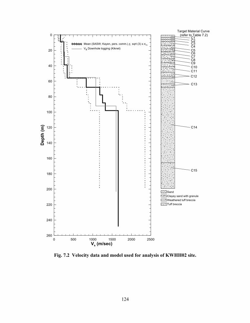
124

0 500 1000 1500 2000 2500Vs (m/sec)

260

240

220

200

180

160

140

120

100

80

60

40

20

0

Dep

th (m

)Mean (SASW; Kayen, pers. comm.) + sqrt (3) x σVs

Vs Downhole logging (Kiknet)

SandClayey sand with granuleWeathered tuff brecciaTuff breccia


C1C2C3C4C5C6

C13

C7C8C9C10C11C12

C15

C14

Fig. 7.2 Velocity data and model used for analysis of KWHH02 site.

125

0 100 200 300 400 500Vs (m/sec)

50

40

30

20

10

0

Dep

th (m

)Mean (EPRI, 1993) + sqrt (3) x σVs

Clayey siltSilty sandClayey silt & sandy siltGravel


C1

C2

C3

Decayed wood & organic matterClayey silt & silty claySilty sand & sandy silt

Fig. 7.3 Velocity data and model used for analysis of Lotung site.

126

Fig. 7.4 Variation of standard deviation and correlation coefficient with depth for generic and site-specific site profiles (Toro 1997).

Table 7.1 Target material curves for La Cienega.

Target Material Curve # Description SourceC1 La Cienega: UCLA Sample L1-1, 4.9 m ROSRINEC2 La Cienega: UCLA Sample L2-2, 6.4 m ROSRINEC3 La Cienega: UCLA Sample S-5, 7.9 m ROSRINEC4 Upper bound sand G/Gmax curve and lower bound sand damping curve Seed et al. (1984)C5 La Cienega: UT Sample L, 36 m ROSRINEC6 La Cienega: UT Sample Q, 52.4 m ROSRINEC7 Sand for 76.5 - 152.4 m EPRI (1993)C8 La Cienega: UT Sample M, 94.5 m ROSRINEC9 La Cienega: UT Sample R, 106.7 m ROSRINEC10 La Cienega: UT Sample N, 125 m ROSRINEC11 La Cienega: UT Sample S, 149.7 m ROSRINEC12 La Cienega: UT Sample O, 185.9 m ROSRINEC13 La Cienega: UT Sample P, 241.1 m ROSRINE

127

Table 7.2 Target material curves for KGWH02.

Target Material Curve # Description SourceC1 PI = 0, OCR = 1, freq = 2 Hz, Num. Cycle = 10, σ0' = 0.28 atm Darendeli (2001)C2 PI = 0, OCR = 1, freq = 2 Hz, Num. Cycle = 10, σ0' = 0.84 atm Darendeli (2001)C3 PI = 0, OCR = 1, freq = 2 Hz, Num. Cycle = 10, σ0' = 1.40 atm Darendeli (2001)C4 PI = 10, OCR = 1, freq = 2 Hz, Num. Cycle = 10, σ0' = 2.06 atm Darendeli (2001)C5 PI = 10, OCR = 1, freq = 2 Hz, Num. Cycle = 10, σ0' = 2.87 atm Darendeli (2001)C6 PI = 10, OCR = 1, freq = 2 Hz, Num. Cycle = 10, σ0' = 3.68 atm Darendeli (2001)C7 PI = 10, OCR = 1, freq = 2 Hz, Num. Cycle = 10, σ0' = 4.49 atm Darendeli (2001)C8 PI = 10, OCR = 1, freq = 2 Hz, Num. Cycle = 10, σ0' = 5.40 atm Darendeli (2001)C9 PI = 10, OCR = 1, freq = 2 Hz, Num. Cycle = 10, σ0' = 6.33 atm Darendeli (2001)C10 PI = 10, OCR = 1, freq = 2 Hz, Num. Cycle = 10, σ0' = 7.28 atm Darendeli (2001)C11 PI = 10, OCR = 1, freq = 2 Hz, Num. Cycle = 10, σ0' = 8.47 atm Darendeli (2001)C12 PI = 10, OCR = 1, freq = 2 Hz, Num. Cycle = 10, σ0' = 9.77 atm Darendeli (2001)C13 PI = 0, OCR = 1, freq = 2 Hz, Num. Cycle = 10, σ0' = 11.63 atm Darendeli (2001)C14 Rock: 76.5 - 152.4 m Silva et al. (1996)C15 Rock: 152.4 - 304.8 m Silva et al. (1996)

Table 7.3 Target material curves for Lotung.

Target Material Curve # Description SourceC1 Lotung: Back Calculation at 6 m Zeghal et al. (1995)C2 Lotung: Back Calculation at 11 m Zeghal et al. (1995)C3 Lotung: Back Calculation at 17 m Zeghal et al. (1995)

128


0

5

10

15

20

25

30

35

Dam

ping

(%)

0

0.1

0.2

0.3

0.4

0.5

0.6

0.7

0.8

0.9

1

G /

Gm

axSilva et al. Rock 0 - 6 mSilva et al. Rock 6 - 15 mSilva et al. Rock 15 - 37 mSilva et al. Rock 37 - 76 mSilva et al. Rock 76 - 152 mSilva et al. Rock 152 - 305 mSilva et al. Rock 305 - 610 mSilva et al. Rock 610 - 1524 mEPRI Sand 6 - 15 mEPRI Sand 76 - 152 mEPRI Sand 152 - 305 mSchnabel (1973) Rock

Fig. 7.5 Material curves for rock developed by Silva et al. (1996).

129

0

0.2

0.4

0.6

0.8

1

G/G

max

0

0.2

0.4

0.6

0.8

1

G/G

max

0

0.2

0.4

0.6

0.8

1

G/G

max

0

0.2

0.4

0.6

0.8

1

G/G

max

0.0001 0.001 0.01 0.1 1 10Cyclic Strain (%)

0.0001 0.001 0.01 0.1 1 10Cyclic Strain (%)

0

0.2

0.4

0.6

0.8

1

G/G

max

Target Curve 1 Target Curve 2 Target Curve 3


Target Curve 7 Target Curve 8

Target Curve 10

0.0001 0.001 0.01 0.1 1 10Cyclic Strain (%)


Target Curve 9

Target Curve 13

Fig. 7.6 Target upper and lower bounds ( 3σ± ) of modulus reduction curve for La

Cienega.

130

0

10

20

30

40

50

Dam

ping

(%)

0

10

20

30

40

50

Dam

ping

(%)

0

10

20

30

40

50

Dam

ping

(%)

0

10

20

30

40

50

Dam

ping

(%)

0.0001 0.001 0.01 0.1 1 10Cyclic Strain (%)

0.0001 0.001 0.01 0.1 1 10Cyclic Strain (%)

0

10

20

30

40

50

Dam

ping

(%)




Target Curve 10

0.0001 0.001 0.01 0.1 1 10Cyclic Strain (%)


Target Curve 9

Target Curve 13

Fig. 7.7 Target upper and lower bounds ( 3σ± ) of damping curves for La Cienega.

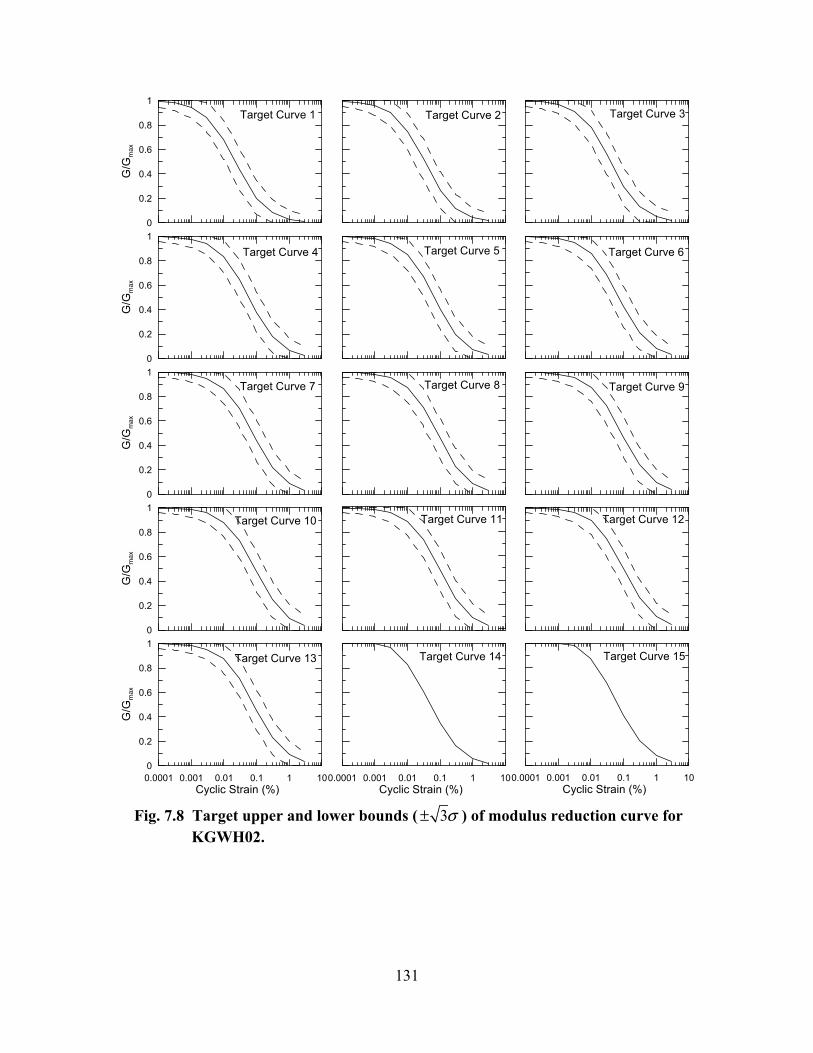
131

0

0.2

0.4

0.6

0.8

1

G/G

max

0

0.2

0.4

0.6

0.8

1

G/G

max

0

0.2

0.4

0.6

0.8

1

G/G

max

0

0.2

0.4

0.6

0.8

1

G/G

max

0.0001 0.001 0.01 0.1 1 10Cyclic Strain (%)

0

0.2

0.4

0.6

0.8

1

G/G

max





Target Curve 9

Target Curve 13

0.0001 0.001 0.01 0.1 1 10Cyclic Strain (%)

Target Curve 14

0.0001 0.001 0.01 0.1 1 10Cyclic Strain (%)

Target Curve 15

Fig. 7.8 Target upper and lower bounds ( 3σ± ) of modulus reduction curve for

KGWH02.

132

0

10

20

30

40

50

Dam

ping

(%)

0

10

20

30

40

50

Dam

ping

(%)

0

10

20

30

40

50

Dam

ping

(%)

0

10

20

30

40

50

Dam

ping

(%)

0.0001 0.001 0.01 0.1 1 10Cyclic Strain (%)

0

10

20

30

40

50

Dam

ping

(%)





Target Curve 9

Target Curve 13

0.0001 0.001 0.01 0.1 1 10Cyclic Strain (%)

Target Curve 14

0.0001 0.001 0.01 0.1 1 10Cyclic Strain (%)

Target Curve 15

Fig. 7.9 Target upper and lower bounds ( 3σ± ) of damping curves for KGWH02.

133

0.0001 0.001 0.01 0.1 1Cyclic Strain (%)

0

0.2

0.4

0.6

0.8

1G

/Gm

ax

0.0001 0.001 0.01 0.1 1Cyclic Strain (%)

0.0001 0.001 0.01 0.1 1Cyclic Strain (%)


mean (Zeghal et al.,1995)± sqrt (3) x σDarendeli

EPRI (1993)

Fig. 7.10 Target upper and lower bounds ( 3σ± ) of modulus reduction curve for Lotung.

0.0001 0.001 0.01 0.1 1Cyclic Strain (%)

0

10

20

30

40

Dam

ping

(%)

0.0001 0.001 0.01 0.1 1Cyclic Strain (%)

0.0001 0.001 0.01 0.1 1Cyclic Strain (%)


mean (Zeghal et al.,1995)± sqrt (3) x σDarendeli EPRI (1993)

Fig. 7.11 Target upper and lower bounds ( 3σ± ) of damping curves for Lotung.

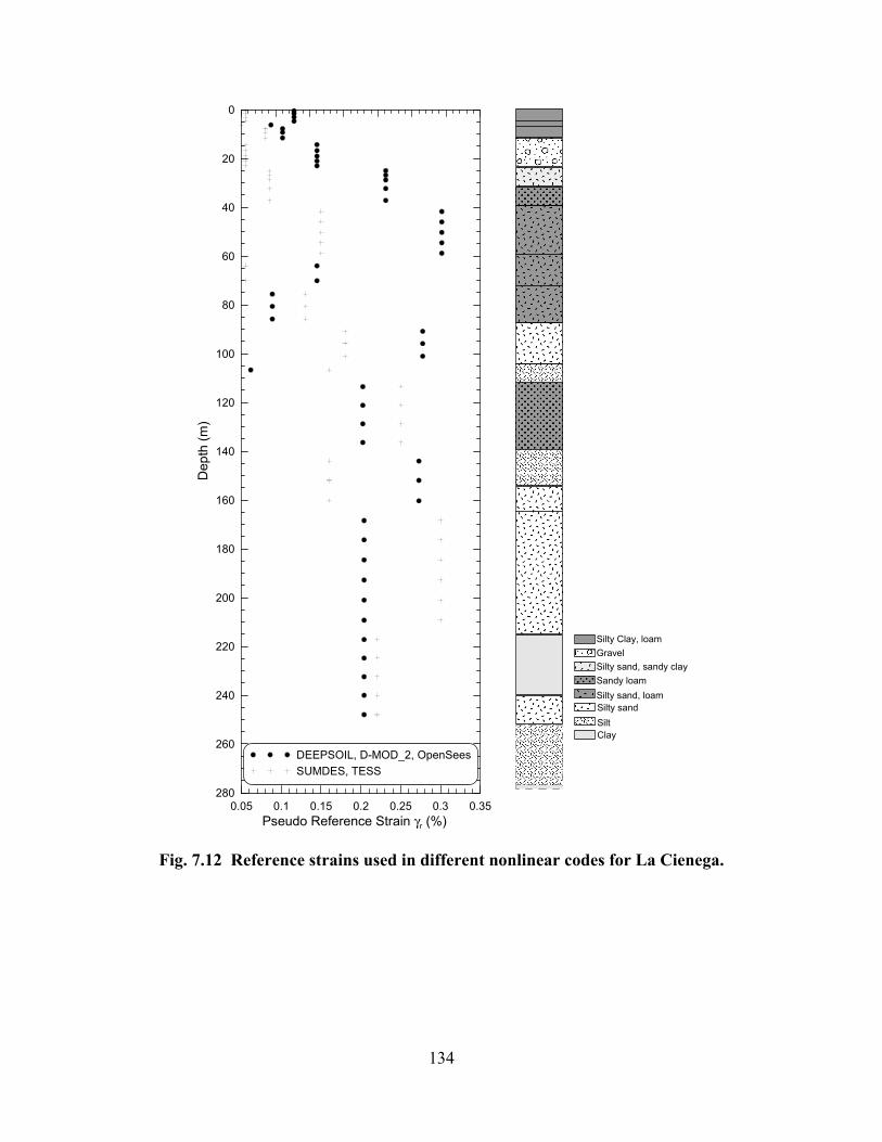
134

0.05 0.1 0.15 0.2 0.25 0.3 0.35Pseudo Reference Strain γr (%)

280

260

240

220

200

180

160

140

120

100

80

60

40

20

0

Dep

th (m

)

DEEPSOIL, D-MOD_2, OpenSeesSUMDES, TESS

Silty Clay, loamGravelSilty sand, sandy claySandy loamSilty sand, loamSilty sandSiltClay

Fig. 7.12 Reference strains used in different nonlinear codes for La Cienega.

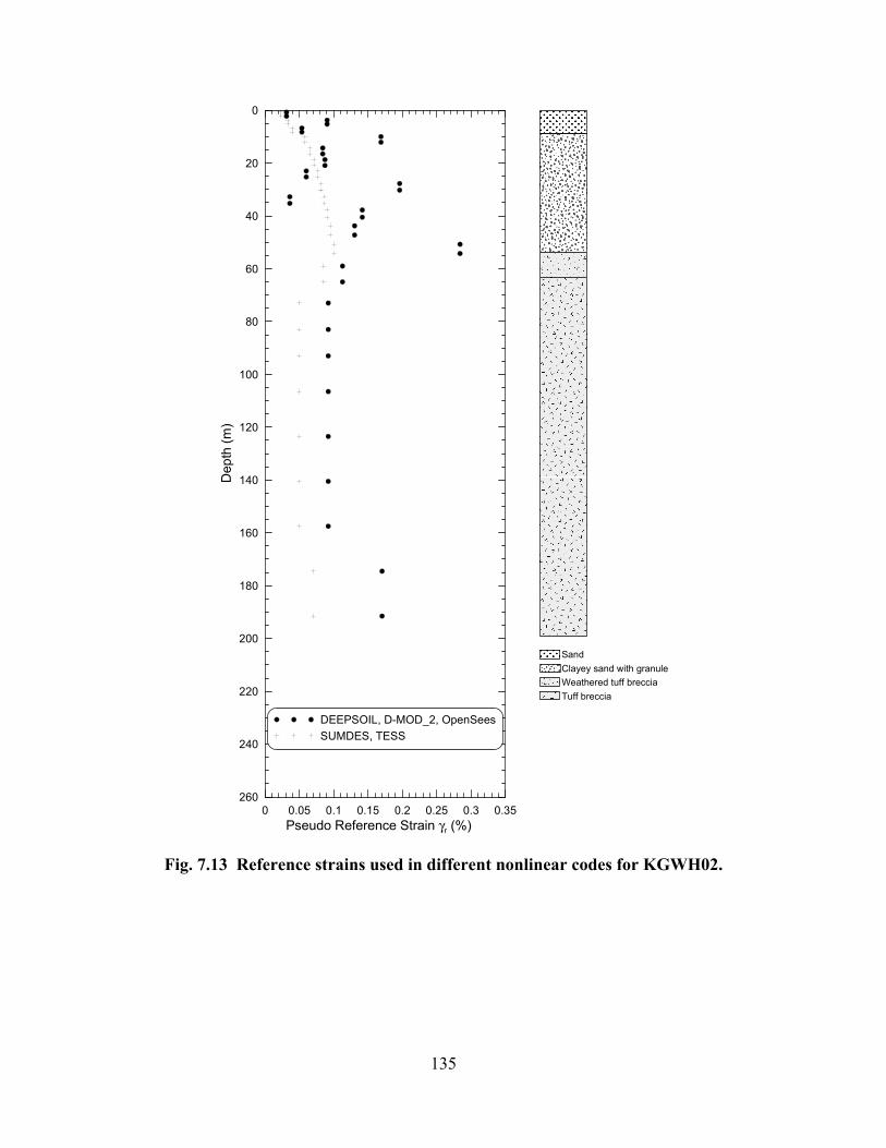
135

0 0.05 0.1 0.15 0.2 0.25 0.3 0.35Pseudo Reference Strain γr (%)

260

240

220

200

180

160

140

120

100

80

60

40

20

0

Dep

th (m

)


SandClayey sand with granuleWeathered tuff brecciaTuff breccia

Fig. 7.13 Reference strains used in different nonlinear codes for KGWH02.

136

0 0.05 0.1 0.15 0.2 0.25 0.3 0.35Pseudo Reference Strain γr (%)

50

40

30

20

10

0

Dep

th (m

)


Clayey siltSilty sandClayey silt & sandy siltGravelDecayed wood & organic matterClayey silt & silty claySilty sand & sandy silt

Fig. 7.14 Reference strains used in different nonlinear codes for Lotung.

137

Table 7.4 Summary of engineering model for La Cienega.

γr (%) β s Viscous Damping (%) γr (%)∗ VT (%) α1 0.9 140 0.26 20.1 1 0.116 1.50 0.70 1.80 0.055 1.80 0.852 1.2 140 0.26 20.1 1 0.116 1.50 0.70 1.80 0.055 1.80 0.853 1.8 180 0.26 20.1 1 0.116 1.50 0.70 1.80 0.055 1.80 0.854 1.5 210 0.23 20.1 1 0.116 1.50 0.70 1.80 0.055 1.80 0.855 1.5 210 0.16 20.1 2 0.087 1.26 0.66 2.50 0.050 2.50 0.856 1.5 240 0.16 20.1 3 0.102 1.10 0.74 1.30 0.080 1.30 0.857 1.5 240 0.16 20.1 3 0.102 1.10 0.74 1.30 0.080 1.30 0.858 3.0 280 0.16 20.1 3 0.102 1.10 0.74 1.30 0.080 1.30 0.859 2.4 310 0.16 20.1 4 0.145 1.74 0.70 0.24 0.055 0.24 0.8510 2.4 310 0.18 20.1 4 0.145 1.74 0.70 0.24 0.055 0.24 0.8511 2.1 290 0.18 20.1 4 0.145 1.74 0.70 0.24 0.055 0.24 0.8512 1.8 350 0.18 20.1 4 0.145 1.74 0.70 0.24 0.055 0.24 0.8513 2.1 370 0.18 20.1 4 0.145 1.74 0.70 0.24 0.055 0.24 0.8514 1.8 340 0.18 20.1 5 0.231 1.70 0.66 1.40 0.085 1.40 0.8515 1.8 314 0.18 20.1 5 0.231 1.70 0.66 1.40 0.085 1.40 0.8516 2.1 314 0.18 20.1 5 0.231 1.70 0.66 1.40 0.085 1.40 0.8517 4.9 472 0.18 20.1 5 0.231 1.70 0.66 1.40 0.085 1.40 0.8518 4.9 472 0.18 20.1 5 0.231 1.70 0.66 1.40 0.085 1.40 0.8519 4.3 411 0.18 20.1 6 0.302 1.50 0.70 1.44 0.150 1.44 0.8520 4.3 411 0.18 20.1 6 0.302 1.50 0.70 1.44 0.150 1.44 0.8521 4.3 411 0.13 20.1 6 0.302 1.50 0.70 1.44 0.150 1.44 0.8522 4.3 411 0.10 20.1 6 0.302 1.50 0.70 1.44 0.150 1.44 0.8523 4.3 411 0.10 20.1 6 0.302 1.50 0.70 1.44 0.150 1.44 0.8524 6.1 625 0.10 20.1 4 0.145 1.74 0.70 0.24 0.055 0.24 0.8525 6.1 625 0.10 20.1 4 0.145 1.74 0.70 0.24 0.055 0.24 0.8526 4.9 518 0.10 20.1 7 0.089 0.66 0.74 0.70 0.130 0.70 0.8527 5.2 518 0.10 20.1 7 0.089 0.66 0.74 0.70 0.130 0.70 0.8528 5.2 518 0.10 20.1 7 0.089 0.66 0.74 0.70 0.130 0.70 0.8529 4.9 518 0.10 20.1 8 0.278 1.10 0.62 0.80 0.180 0.80 0.8530 5.2 518 0.10 20.1 8 0.278 1.10 0.62 0.80 0.180 0.80 0.8531 5.2 518 0.11 20.1 8 0.278 1.10 0.62 0.80 0.180 0.80 0.8532 6.1 518 0.12 20.1 9 0.062 0.42 0.78 1.45 0.160 1.45 0.8033 7.6 561 0.12 20.1 10 0.202 0.74 0.66 0.60 0.250 0.60 0.8534 7.6 561 0.12 20.1 10 0.202 0.74 0.66 0.60 0.250 0.60 0.8535 7.6 561 0.12 20.1 10 0.202 0.74 0.66 0.60 0.250 0.60 0.8536 7.6 561 0.12 20.1 10 0.202 0.74 0.66 0.60 0.250 0.60 0.8537 7.6 561 0.12 20.1 11 0.273 1.30 0.74 2.00 0.160 2.00 0.8038 8.2 561 0.12 20.1 11 0.273 1.30 0.74 2.00 0.160 2.00 0.8039 8.5 561 0.12 20.1 11 0.273 1.30 0.74 2.00 0.160 2.00 0.8040 7.6 600 0.12 20.1 12 0.204 0.70 0.66 1.10 0.300 1.10 0.8541 8.2 600 0.12 20.1 12 0.204 0.70 0.66 1.10 0.300 1.10 0.8542 8.2 600 0.12 20.1 12 0.204 0.70 0.66 1.10 0.300 1.10 0.8543 8.2 600 0.12 20.1 12 0.204 0.70 0.66 1.10 0.300 1.10 0.8544 8.2 600 0.12 20.1 12 0.204 0.70 0.66 1.10 0.300 1.10 0.8545 8.2 600 0.12 20.1 12 0.204 0.70 0.66 1.10 0.300 1.10 0.8546 7.6 640 0.12 20.1 13 0.204 0.74 0.66 0.65 0.220 0.65 0.8547 7.6 640 0.12 20.1 13 0.204 0.74 0.66 0.65 0.220 0.65 0.8548 7.6 640 0.12 20.1 13 0.204 0.74 0.66 0.65 0.220 0.65 0.8549 7.6 640 0.12 20.1 13 0.204 0.74 0.66 0.65 0.220 0.65 0.8550 8.2 640 0.12 20.1 13 0.204 0.74 0.66 0.65 0.220 0.65 0.85

* Also used in SUMDES

Fitted Curves for D-MOD_2, DEEPSOIL and OpenSees Fitted Curves for TESSLayer # Thickness (m) Vs (m/s) σVs ( ln(m/s) ) Unit Weight (kN/m3) Target Material Curve

138

Table 7.5 Summary of engineering model for Kiknet KGWH02.

γr (%) β s Viscous Damping (%) γr (%)∗ VT (%) α1 1.5 163 0.26 18.9 1 0.031 1.18 0.66 1.45 0.023 1.45 0.852 1.5 163 0.26 18.9 1 0.031 1.18 0.66 1.45 0.023 1.45 0.853 1.5 163 0.26 18.9 2 0.090 1.86 0.70 1.05 0.033 1.05 0.854 1.5 163 0.16 18.9 2 0.090 1.86 0.70 1.05 0.033 1.05 0.855 1.5 163 0.16 18.9 3 0.054 1.14 0.70 0.91 0.040 0.91 0.856 1.5 163 0.16 18.9 3 0.054 1.14 0.70 0.91 0.040 0.91 0.857 2.0 249 0.16 18.9 4 0.169 1.94 0.70 0.93 0.058 0.93 0.858 2.2 249 0.16 18.9 4 0.169 1.94 0.70 0.93 0.058 0.93 0.859 2.2 249 0.16 18.9 5 0.084 1.10 0.70 0.85 0.065 0.85 0.8510 2.2 249 0.18 18.9 5 0.084 1.10 0.70 0.85 0.065 0.85 0.8511 2.2 249 0.18 18.9 6 0.087 1.06 0.70 0.79 0.071 0.79 0.8512 2.2 249 0.18 18.9 6 0.087 1.06 0.70 0.79 0.071 0.79 0.8513 2.0 262 0.18 18.9 7 0.060 0.78 0.70 0.74 0.076 0.74 0.8514 2.5 262 0.18 18.9 7 0.060 0.78 0.70 0.74 0.076 0.74 0.8515 2.5 262 0.18 18.9 8 0.196 1.70 0.70 0.70 0.081 0.70 0.8516 2.5 262 0.18 18.9 8 0.196 1.70 0.70 0.70 0.081 0.70 0.8517 2.5 262 0.18 18.9 9 0.036 0.50 0.70 0.67 0.086 0.67 0.8518 2.5 262 0.18 18.9 9 0.036 0.50 0.70 0.67 0.086 0.67 0.8519 2.5 262 0.18 18.9 10 0.142 1.26 0.70 0.64 0.090 0.64 0.8520 3.0 336 0.18 18.9 10 0.142 1.26 0.70 0.64 0.090 0.64 0.8521 3.5 336 0.18 18.9 11 0.130 1.14 0.70 0.62 0.095 0.62 0.8522 3.5 336 0.18 18.9 11 0.130 1.14 0.70 0.62 0.095 0.62 0.8523 3.5 336 0.10 18.9 12 0.284 1.90 0.70 0.59 0.100 0.59 0.8524 3.5 336 0.10 18.9 12 0.284 1.90 0.70 0.59 0.100 0.59 0.8525 6.0 836 0.20 20.4 13 0.113 1.14 0.70 0.49 0.085 0.49 0.8526 6.0 836 0.20 20.4 13 0.113 1.14 0.70 0.49 0.085 0.49 0.8527 10.0 1183 0.20 21.2 14 0.092 1.42 0.78 3.17 0.050 3.17 0.8528 10.0 1252 0.20 21.2 14 0.092 1.42 0.78 3.17 0.050 3.17 0.8529 10.0 1329 0.20 21.2 14 0.092 1.42 0.78 3.17 0.050 3.17 0.8530 17.0 1661 0.20 21.2 14 0.092 1.42 0.78 3.17 0.050 3.17 0.8531 17.0 1661 0.20 21.2 14 0.092 1.42 0.78 3.17 0.050 3.17 0.8532 17.0 1661 0.20 21.2 14 0.092 1.42 0.78 3.17 0.050 3.17 0.8533 17.0 1661 0.20 21.2 14 0.092 1.42 0.78 3.17 0.050 3.17 0.8534 17.0 1661 0.20 21.2 15 0.170 1.82 0.78 3.13 0.070 3.13 0.8535 17.0 1661 0.20 21.2 15 0.170 1.82 0.78 3.13 0.070 3.13 0.85


Unit Weight (kN/m3) Target Material Curve Fitted Curves for D-MOD_2, DEEPSOIL and OpenSees Fitted Curves for TESSLayer # Thickness (m) Vs (m/s) σVs ( ln(m/s) )

Table 7.6 Summary of engineering model for Lotung.

γr (%) β s Viscous Damping (%) γr (%)∗ VT (%) α1 0.8 114 0.26 17.6 1 0.097 2.06 0.78 1.00 0.037 1.00 0.852 0.8 114 0.26 17.6 1 0.097 2.06 0.78 1.00 0.037 1.00 0.853 0.8 114 0.26 17.6 1 0.097 2.06 0.78 1.00 0.037 1.00 0.854 0.7 121 0.26 17.6 1 0.097 2.06 0.78 1.00 0.037 1.00 0.855 0.7 121 0.26 17.6 1 0.097 2.06 0.78 1.00 0.037 1.00 0.856 0.3 121 0.26 17.6 1 0.097 2.06 0.78 1.00 0.037 1.00 0.857 1.4 149 0.22 17.6 1 0.097 2.06 0.78 1.00 0.037 1.00 0.858 0.5 149 0.15 17.6 1 0.097 2.06 0.78 1.00 0.037 1.00 0.859 0.7 149 0.15 17.6 2 0.089 2.02 0.74 1.00 0.034 1.00 0.8510 1.3 165 0.15 18.1 2 0.089 2.02 0.74 1.00 0.034 1.00 0.8511 1.0 165 0.15 18.1 2 0.089 2.02 0.74 1.00 0.034 1.00 0.8512 1.0 180 0.15 18.1 2 0.089 2.02 0.74 1.00 0.034 1.00 0.8513 1.0 180 0.15 18.1 2 0.089 2.02 0.74 1.00 0.034 1.00 0.8514 0.2 180 0.15 17.6 3 0.026 0.86 0.66 1.50 0.032 1.50 0.8515 1.5 185 0.15 17.6 3 0.026 0.86 0.66 1.50 0.032 1.50 0.8516 1.5 185 0.15 17.6 3 0.026 0.86 0.66 1.50 0.032 1.50 0.8517 1.4 189 0.16 17.6 3 0.026 0.86 0.66 1.50 0.032 1.50 0.8518 1.4 189 0.17 17.6 3 0.026 0.86 0.66 1.50 0.032 1.50 0.8519 0.3 189 0.17 19.7 3 0.026 0.86 0.66 1.50 0.032 1.50 0.8520 1.3 235 0.17 19.7 3 0.026 0.86 0.66 1.50 0.032 1.50 0.8521 1.3 235 0.17 19.7 3 0.026 0.86 0.66 1.50 0.032 1.50 0.8522 2.3 244 0.17 19.7 3 0.026 0.86 0.66 1.50 0.032 1.50 0.8523 1.6 244 0.17 18.7 3 0.026 0.86 0.66 1.50 0.032 1.50 0.8524 1.8 222 0.17 18.7 3 0.026 0.86 0.66 1.50 0.032 1.50 0.8525 1.9 228 0.17 18.7 3 0.026 0.86 0.66 1.50 0.032 1.50 0.8526 1.9 228 0.17 18.7 3 0.026 0.86 0.66 1.50 0.032 1.50 0.8527 0.4 319 0.17 18.7 3 0.026 0.86 0.66 1.50 0.032 1.50 0.8528 2.0 319 0.17 18.7 3 0.026 0.86 0.66 1.50 0.032 1.50 0.8529 2.1 319 0.17 18.7 3 0.026 0.86 0.66 1.50 0.032 1.50 0.8530 1.9 248 0.17 18.7 3 0.026 0.86 0.66 1.50 0.032 1.50 0.8531 1.1 248 0.17 18.7 3 0.026 0.86 0.66 1.50 0.032 1.50 0.8532 2.1 259 0.17 17.6 3 0.026 0.86 0.66 1.50 0.032 1.50 0.8533 1.9 251 0.17 17.6 3 0.026 0.86 0.66 1.50 0.032 1.50 0.8534 1.9 251 0.17 17.6 3 0.026 0.86 0.66 1.50 0.032 1.50 0.8535 2.1 256 0.17 19.7 3 0.026 0.86 0.66 1.50 0.032 1.50 0.8536 2.1 256 0.17 19.7 3 0.026 0.86 0.66 1.50 0.032 1.50 0.85


Unit Weight (kN/m3) Target Material Curve Fitted Curves for D-MOD_2, DEEPSOIL and OpenSees Fitted Curves for TESSLayer # Thickness (m) Vs (m/s) σVs ( ln(m/s) )

139

-0.2

0

0.2A

ccel

erat

ion

(g)

Surface - EW

-0.2

0

0.2

Acc

eler

atio

n (g

)

18.3 m - EW

-0.2

0

0.2

Acc

eler

atio

n (g

)

100.6 m - EW

-0.2

0

0.2

Acc

eler

atio

n (g

)

252.1 m - EW

-0.4-0.2

00.20.4

Acc

eler

atio

n (g

)

Surface - NS

-0.4-0.2

00.20.4

Acc

eler

atio

n (g

)

18.3 m - NS

-0.4-0.2

00.20.4

Acc

eler

atio

n (g

)

100.6 m - NS

0 5 10 15 20Time (sec)

-0.4-0.2

00.20.4

Acc

eler

atio

n (g

)

252.1 m - NS

Fig. 7.15 Acceleration histories recorded at La Cienega array.

140

-0.2

0

0.2A

ccel

erat

ion

(g)

Surface - EW

-0.2

0

0.2

Acc

eler

atio

n (g

)

200 m - EW

-0.2

0

0.2

Acc

eler

atio

n (g

)

Surface - NS

15 20 25 30 35 40 45 50 55 60 65Time (sec)

-0.2

0

0.2

Acc

eler

atio

n (g

)

200 m - NS

Fig. 7.16 Acceleration histories recorded at Kiknet KGWH02 array.

141

-0.2

-0.1

0

0.1

0.2

Acc

eler

atio

n (g

) Surface - EW

-0.2

-0.1

0

0.1

0.2

Acc

eler

atio

n (g

) 6 m - EW

-0.2

-0.1

0

0.1

0.2

Acc

eler

atio

n (g

) 11 m - EW

-0.2

-0.1

0

0.1

0.2

Acc

eler

atio

n (g

) 17 m - EW

0 5 10 15 20 25 30 35Time (sec)

-0.2

-0.1

0

0.1

0.2

Acc

eler

atio

n (g

) 47 m - EW

(a)

Fig. 7.17 Acceleration histories for (a) EW direction recorded at Lotung array and (b) NS direction recorded at Lotung array.

142

-0.2

-0.1

0

0.1

0.2

Acc

eler

atio

n (g

) Surface - NS

-0.2

-0.1

0

0.1

0.2

Acc

eler

atio

n (g

) 6 m - NS

-0.2

-0.1

0

0.1

0.2

Acc

eler

atio

n (g

) 11 m - NS

-0.2

-0.1

0

0.1

0.2

Acc

eler

atio

n (g

) 17 m - NS

0 5 10 15 20 25 30 35Time (sec)

-0.2

-0.1

0

0.1

0.2

Acc

eler

atio

n (g

) 47 m - NS

(b)

Fig. 7.17—Continued.

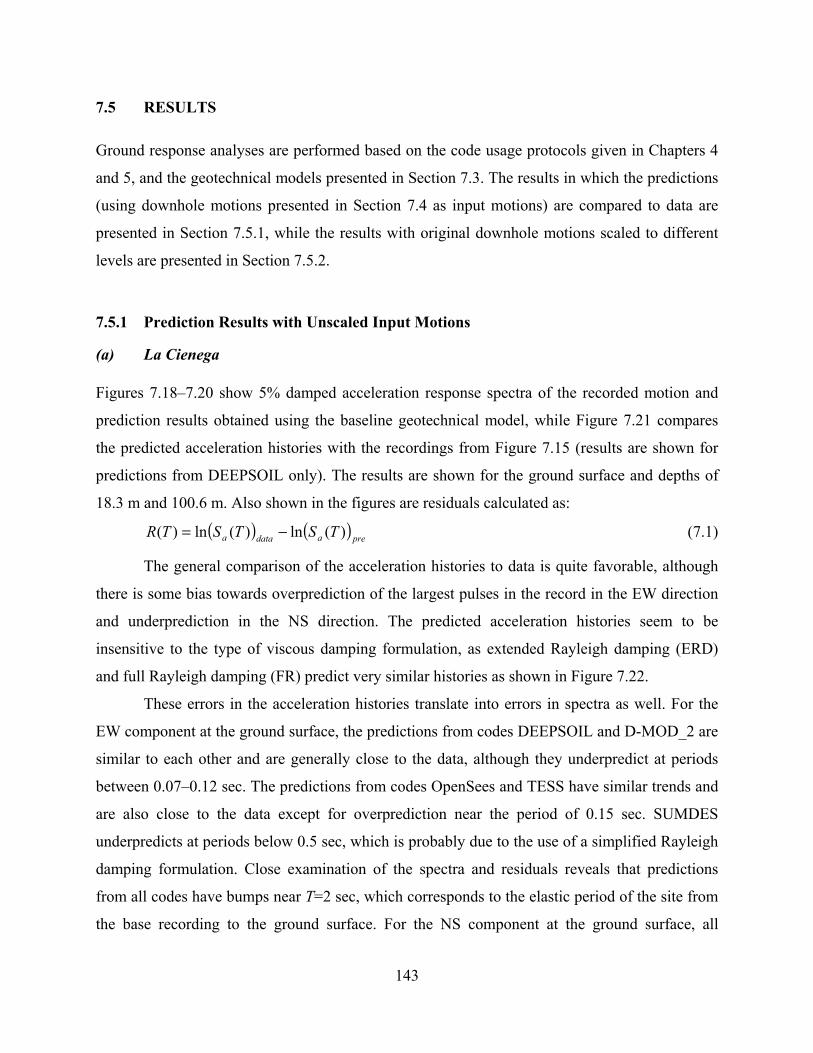
143

7.5 RESULTS

Ground response analyses are performed based on the code usage protocols given in Chapters 4

and 5, and the geotechnical models presented in Section 7.3. The results in which the predictions

(using downhole motions presented in Section 7.4 as input motions) are compared to data are

presented in Section 7.5.1, while the results with original downhole motions scaled to different

levels are presented in Section 7.5.2.

7.5.1 Prediction Results with Unscaled Input Motions

(a) La Cienega

Figures 7.18–7.20 show 5% damped acceleration response spectra of the recorded motion and

prediction results obtained using the baseline geotechnical model, while Figure 7.21 compares

the predicted acceleration histories with the recordings from Figure 7.15 (results are shown for

predictions from DEEPSOIL only). The results are shown for the ground surface and depths of

18.3 m and 100.6 m. Also shown in the figures are residuals calculated as:

( ) ( )preadataa TSTSTR )(ln)(ln)( −= (7.1)

The general comparison of the acceleration histories to data is quite favorable, although

there is some bias towards overprediction of the largest pulses in the record in the EW direction

and underprediction in the NS direction. The predicted acceleration histories seem to be

insensitive to the type of viscous damping formulation, as extended Rayleigh damping (ERD)

and full Rayleigh damping (FR) predict very similar histories as shown in Figure 7.22.

These errors in the acceleration histories translate into errors in spectra as well. For the

EW component at the ground surface, the predictions from codes DEEPSOIL and D-MOD_2 are

similar to each other and are generally close to the data, although they underpredict at periods

between 0.07–0.12 sec. The predictions from codes OpenSees and TESS have similar trends and

are also close to the data except for overprediction near the period of 0.15 sec. SUMDES

underpredicts at periods below 0.5 sec, which is probably due to the use of a simplified Rayleigh

damping formulation. Close examination of the spectra and residuals reveals that predictions

from all codes have bumps near T=2 sec, which corresponds to the elastic period of the site from

the base recording to the ground surface. For the NS component at the ground surface, all

144

nonlinear codes underpredict at periods below 0.5 sec. The misfits of predictions relative to data

at depths of 18.3 m and 100.6 m follow similar trends to those at the ground surface.

The importance of fitting strategy is studied by using model curves obtained from the

“MR” and “MRD” fitting approaches described in Section 4.2. Only DEEPSOIL is used for this

study. The prediction results for ground surface motions calculated using both fitting approaches

are compared in Figure 7.22. It can be observed that results from both approaches are very

similar, which is probably due to the fact that the input motions used here are relatively modest

and do not introduce large soil nonlinearity. That is, the strain experienced by the soil is small,

and the model damping curves from both “MRD” and “MR” fitting approaches are similar for

small-strain conditions.

OpenSees and SUMDES are formulated using a 3D finite element framework and are

capable of simulating ground response with input motions from both horizontal and vertical

components specified simultaneously. To study the 2D effect in ground response, input motions

from both horizontal directions are specified simultaneously. Only OpenSees is used in this

study. The prediction results for ground surface obtained from 1D and 2D simulations are

compared in Figure 7.24. It is observed that the response for the NS direction is reduced when

the 2D effect is considered. This is because the NS direction of the input motion is the stronger

component, and the wave energy would be diverted to the EW direction when shaking in both

directions is allowed to happen simultaneously.

Model-to-model variability is evaluated for the ground surface results in Figure 7.18. For

period T, the median estimate ( ))(ln TSa is first evaluated from the five nonlinear model

predictions. Model variability, σm, is then calculated from the variance as follows:

( )( ) ( ) 2

,2

ln ( ) ln ( )( ) ( )

1

a apre ii

m a pre

S T S TT Var S T

Nσ

⎡ ⎤−⎣ ⎦= =

−

∑ (7.2)

where N = number of predictions (five). Figure 7.25 shows the variation of σm with period.

The variability in prediction results from uncertain shear wave velocity and uncertain

modulus reduction and damping curves is considered. The variability in the velocity profile that

was used in the analysis is shown in Figure 7.1, while the variability in material curves is shown

in Figures 7.6–7.7. The response variability due to material uncertainty is assessed using

DEEPSOIL predictions only. To calculate the standard deviation due to velocity, ground motions

145

are predicted based on two non-baseline velocity profiles (mean + 3 standard deviation

velocities and mean - 3 standard deviation velocities). The standard deviation of the ground

motions due to the variability in velocity (denoted σv) is estimated according to the FOSM

method (Baker and Cornell 2003; Melchers 1999), as follows: 3

2

1(ln( ( ) ln( ( ))v i i

iw Sa T Sa Tσ

=

= −∑ (7.3)

where

1 :

2 : 3

3 : 3

3

1

1 2 3

( ) ( )

( ) ( )

( ) ( )

ln( ( )) ln( ( ) )

2 / 3; w w 1/ 6

s

s Vs

s Vs

a V

a V

a V

a i a ii

Sa T S T

Sa T S T

Sa T S T

S T w S T

w

μ

μ σ

μ σ

+

−

=

=

=

=

=

= = =

∑

(7.4)

The standard deviation due to the variability in material curves (denoted σG) is estimated

similarly to σv. Figure 7.25 shows the estimated standard deviation in prediction due to different

sources of variability. At periods below 0.4 sec, the model and material curve variability

dominate, while the velocity variability is strongest at periods above 0.4 sec.

0.0

0.2

0.4

0.6

0.8

1.0

1.2

1.4

1.6

Sa (g

)

Downhole rock record (252.1 m)Surface Record


-0.8

-0.4

0.0

0.4

0.8

1.2

1.6

Res

idua

l, R

(ln

units

) DEEPSOILD-MOD_2OpenSeesSUMDESTESSSHAKE2004

(a) Surface-EW


(b) Surface-NS

(c) Surface-EW (d) Surface-NS


direct spectral ordinates and prediction residuals for ground surface. Results shown for two horizontal directions.

146

0.0

0.2

0.4

0.6

Sa

(g)

Downhole rock record (252.1 m)Downhole record (18.3 m)


-1.2

-0.8

-0.4

0.0

0.4

0.8

1.2

1.6

Res

idua

l, R

(ln

units

) DEEPSOILD-MOD_2OpenSeesSUMDESTESSSHAKE2004

(a) 18.3 m-EW


(b) 18.3 m-NS

(c) 18.3 m-EW (d) 18.3 m-NS


direct spectral ordinates and prediction residuals for 18.3 m.

0.0

0.2

0.4

0.6

Sa (g

)

Downhole rock record (252.1 m)Downhole record (100.6 m)


-1.2

-0.8

-0.4

0.0

0.4

0.8

1.2

1.6

Res

idua

l, R

(ln

units

)


(a) 100.6 m-EW


(b) 100.6 m-NS

(c) 100.6 m-EW (d) 100.6 m-NS


direct spectral ordinates and prediction residuals for 100.6 m.

147

-0.2

0

0.2

Acc

eler

atio

n (g

)

RecordedPredicted by DEEPSOIL

Surface - EW

-0.2

0

0.2

Acc

eler

atio

n (g

)

18.3 m - EW

-0.2

0

0.2

Acc

eler

atio

n (g

)

100.6 m - EW

-0.2

0

0.2

Acc

eler

atio

n (g

)

252.1 m - EW

-0.4-0.2

00.20.4

Acc

eler

atio

n (g

)

Surface - NS

-0.4-0.2

00.20.4

Acc

eler

atio

n (g

)

18.3 m - NS

-0.4-0.2

00.20.4

Acc

eler

atio

n (g

)

100.6 m - NS

5 10 15Time (sec)

-0.4-0.2

00.20.4

Acc

eler

atio

n (g

)

252.1 m - NS

Fig. 7.21 Acceleration histories for data and simulation results from DEEPSOIL for

ground surface.

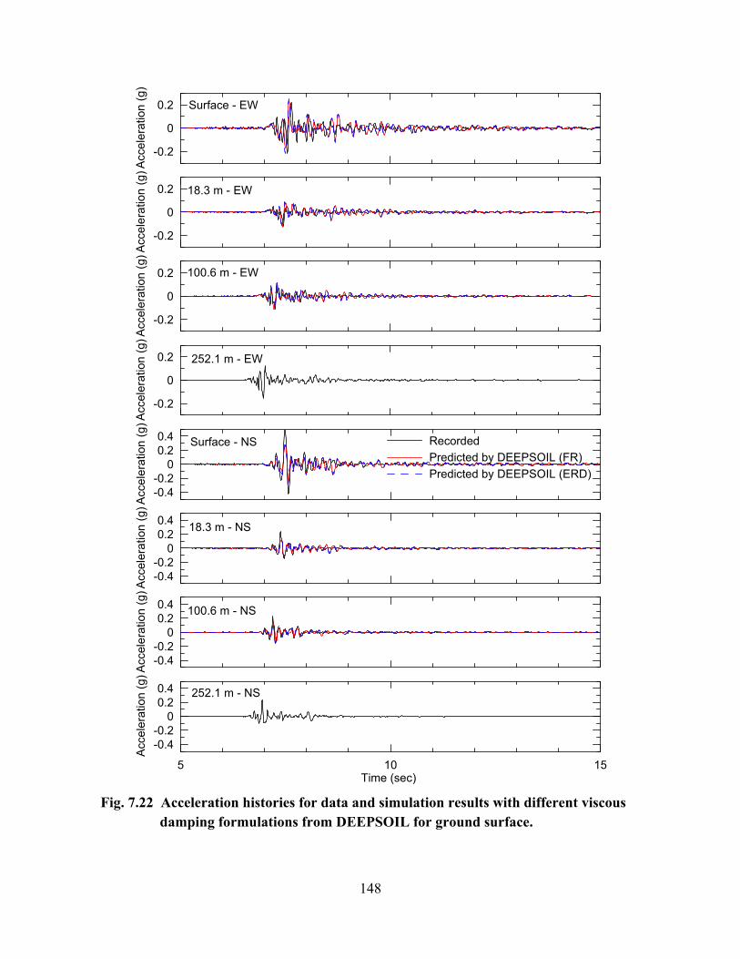
148

-0.2

0

0.2

Acc

eler

atio

n (g

)

RecordedPredicted by DEEPSOIL (FR)Predicted by DEEPSOIL (ERD)

Surface - EW

-0.2

0

0.2

Acc

eler

atio

n (g

)

18.3 m - EW

-0.2

0

0.2

Acc

eler

atio

n (g

)

100.6 m - EW

-0.2

0

0.2

Acc

eler

atio

n (g

)

252.1 m - EW

-0.4-0.2

00.20.4

Acc

eler

atio

n (g

)

Surface - NS

-0.4-0.2

00.20.4

Acc

eler

atio

n (g

)

18.3 m - NS

-0.4-0.2

00.20.4

Acc

eler

atio

n (g

)

100.6 m - NS

5 10 15Time (sec)

-0.4-0.2

00.20.4

Acc

eler

atio

n (g

)

252.1 m - NS

Fig. 7.22 Acceleration histories for data and simulation results with different viscous

damping formulations from DEEPSOIL for ground surface.

149

0.0

0.2

0.4

0.6

0.8

1.0

1.2

1.4

1.6

Sa (g

)



-0.8

-0.4

0.0

0.4

0.8

1.2

1.6

Res

idua

l, R

(ln

units

) DEEPSOIL ("MRD" Fitting)DEEPSOIL ("MR" Fitting)

(a) Surface-EW


(b) Surface-NS


Fig. 7.23 Acceleration response spectra for data and simulation results (with model curves

obtained from both “MRD” and “MR” fitting approaches) compared through direct spectral ordinates and prediction residuals for ground surface.

0.0

0.2

0.4

0.6

0.8

1.0

1.2

1.4

1.6

Sa (g

)



-0.8

-0.4

0.0

0.4

0.8

1.2

1.6

Res

idua

l, R

(ln

units

) OpenSees (1D)OpenSees (2D)

(a) Surface-EW


(b) Surface-NS


Fig. 7.24 Acceleration response spectra for data and simulation results (using 1D and 2D

simulation options in OpenSees ) compared through direct spectral ordinates and prediction residuals for ground surface.

150


00.10.20.30.40.50.60.70.80.9

1

Est

imat

ed s

tand

ard

devi

atio

n in

pre

dict

ion

(ln u

nit)

Material Curve variability, σGVelocity variability, σv

Model variability, σmOverall variability, σ

Ts = 2.0 sec

Fig. 7.25 Standard deviation terms associated with geometric mean acceleration response

spectral ordinates for ground surface. Ts denotes elastic site period.

(b) KGWH02

Figure 7.26 shows 5% damped acceleration response spectra of the recorded motion and

prediction results for the ground surface obtained using the baseline geotechnical model, while

Figure 7.27 compares the predicted acceleration histories with the recordings from Figure 7.16

(results are shown for predictions from DEEPSOIL only). The residuals shown in the figure are

calculated using Equation 7.1.

The general comparison of the acceleration histories to data is poor. The data contain a

large amount of high-frequency content that is not well simulated in the predictions. Examining

the response spectra, for T < 0.3 sec, all codes generally underpredict the observed motions in

both the EW and NS directions except for T = 0.04 - 0.09 sec, where residuals are nearly zero for

all codes except SUMDES. For T > 0.3 sec, predictions from all codes are similar to the data

except the bumps near T=0.9 sec, which correspond to the elastic period of the site for the soil

layers only (from the depth of 68 m to the ground surface).

The relative merits of “MR” and “MRD” fitting approaches are also studied using

KGWH02. The prediction results for ground surface motions calculated using both fitting

approaches are compared in Figure 7.28. Similar to the observation from analyses for the La

151

Cienega site, the results from both approaches are very similar due to the modest input ground

motion amplitude.

Two-dimensional effects are studied using OpenSees. The prediction results for ground

surface obtained from 1D and 2D simulations are compared in Figure 7.29. The predictions from

both types of simulations are similar because there is no dominant component in the input

motion.

Model-to-model variability is evaluated for the ground surface results using Equation 7.2.

Figure 7.30 shows the variation of σm with period.

The variability in prediction resulting from uncertain shear wave velocity and uncertain

nonlinear modulus reduction and damping curves is considered. The variability in velocity

profile that was used in the analysis is shown in Figure 7.2, while the variability in material

curves is shown in Figures 7.8 and 7.9. The response variability due to material uncertainty is

assessed using DEEPSOIL predictions only. The standard deviation due to velocity and material

curves are calculated in the same way as for La Cienega. It should be mentioned that the

variability of material curve for rock and soil is considered to be independent of each other. It is

found that variability in rock material curves has only a slight effect on the predictions at T < 0.1

sec and no discernable effect for other period ranges. Accordingly, the estimated total standard

deviation excludes the uncertainty in predictions due to rock material curves. Figure 7.30 shows

the estimated standard deviation in prediction due to different sources of variability.

For T < 0.15 sec, the (soil) material curve variability dominates, while velocity (whole

profile) variability dominates for T > 0.15 sec. Standard deviation due to model variability is

generally small compared to other sources of variability except in the period range T = 0.05 - 0.1

sec (where the standard deviation is large due to SUMDES being significantly different from the

other codes). Analyses are also performed for which only the velocity of upper 9 m of soil is

varied to mean + 3 standard deviation velocities. Focusing velocity variability in the upper

portion of the profile increases σv for T < 0.5 sec and decreases σv for longer periods. Figure 7.31

compares the 5% damped acceleration response spectra and the residuals calculated for different

velocity profiles.

152

0.0

0.2

0.4

0.6

0.8

1.0

Sa

(g)

Downhole rock record (200 m)Surface Record


-1.6

-1.2

-0.8

-0.4

0.0

0.4

0.8

1.2

Res

idua

l, R

(ln

units

)


(a) Surface-EW


(b) Surface-NS



direct spectral ordinates and prediction residuals for ground surface.

-0.2

0

0.2

Acc

eler

atio

n (g

)

Surface - EW

-0.2

0

0.2

Acc

eler

atio

n (g

)

200 m - EW

-0.2

0

0.2

Acc

eler

atio

n (g

)

Surface - NS

15 20 25 30 35 40 45Time (sec)

-0.2

0

0.2

Acc

eler

atio

n (g

)

200 m - NS

Fig. 7.27 Acceleration histories for data and simulation results from DEEPSOIL for

ground surface.

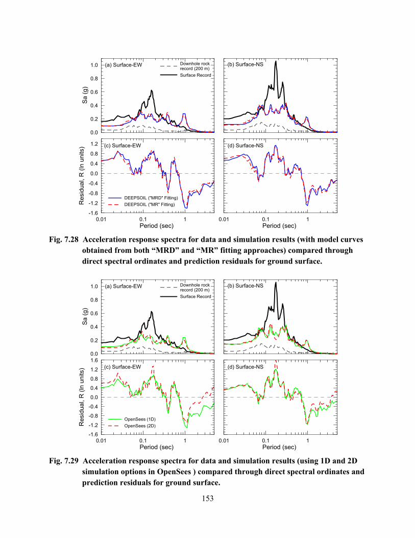
153

0.0

0.2

0.4

0.6

0.8

1.0

Sa

(g)



-1.6

-1.2

-0.8

-0.4

0.0

0.4

0.8

1.2

Res

idua

l, R

(ln

units

)

DEEPSOIL ("MRD" Fitting)DEEPSOIL ("MR" Fitting)

(a) Surface-EW


(b) Surface-NS


Fig. 7.28 Acceleration response spectra for data and simulation results (with model curves

obtained from both “MRD” and “MR” fitting approaches) compared through direct spectral ordinates and prediction residuals for ground surface.

0.0

0.2

0.4

0.6

0.8

1.0

Sa

(g)



-1.6

-1.2

-0.8

-0.4

0.0

0.4

0.8

1.2

1.6

Res

idua

l, R

(ln

units

)

OpenSees (1D)OpenSees (2D)

(a) Surface-EW


(b) Surface-NS


Fig. 7.29 Acceleration response spectra for data and simulation results (using 1D and 2D

simulation options in OpenSees ) compared through direct spectral ordinates and prediction residuals for ground surface.

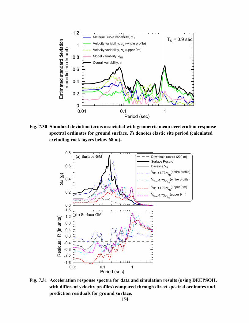
154


0

0.2

0.4

0.6

0.8

1

1.2

Est

imat

ed s

tand

ard

devi

atio

n in

pre

dict

ion

(ln u

nit)

Material Curve variability, σGVelocity variability, σv (whole profile)

Velocity variability, σv (upper 9m)


Ts = 0.9 sec


spectral ordinates for ground surface. Ts denotes elastic site period (calculated excluding rock layers below 68 m)..

0.0

0.2

0.4

0.6

0.8

Sa

(g)

Downhole record (200 m)Surface Record Baseline VsVs:μ+1.73σvs

(entire profile)

Vs:μ-1.73σvs(entire profile)

Vs:μ+1.73σvs(upper 9 m)

Vs:μ-1.73σvs(upper 9 m)


-1.6

-1.2

-0.8

-0.4

0.0

0.4

0.8

1.2

1.6

Res

idua

l, R

(ln

units

)

(a) Surface-GM

(b) Surface-GM

Fig. 7.31 Acceleration response spectra for data and simulation results (using DEEPSOIL

with different velocity profiles) compared through direct spectral ordinates and prediction residuals for ground surface.

155

(c) Lotung

Figures 7.32–7.35 show 5% damped acceleration response spectra of the recorded motion and

predictions obtained using the baseline geotechnical model, while Figure 7.36 compares the

predicted acceleration histories with the recordings from Figure 7.17 (results are shown for

predictions from DEEPSOIL only). The results are shown for the ground surface and depths of 6,

11, and 17 m. The residuals shown in the figure are calculated using Equation 7.1.

The general comparison of the acceleration histories to data is quite favorable, although

there is some bias towards underprediction of the largest pulses These errors in the acceleration

histories translate into errors in spectra as well. For both EW and NS components at the ground

surface, the predictions from all of the codes are generally similar to each other and underpredict

at periods below 0.7 sec. The misfits of predictions relative to data at depths of 6 m, 11 m, and

17 m follow similar trends to those at the ground surface. One unusual feature is that large

spectral accelerations at high frequency are predicted at depth by OpenSees which are

incompatible with the data.

Model-to-model variability is evaluated for the ground surface results using Equation 7.2.

Figure 7.37 shows the variation of σm with period.

The variability in prediction resulting from uncertain shear wave velocity and uncertain

nonlinear modulus reduction and damping curves is considered. The variability in velocity

profile that was used in the analysis is shown in Figure 7.3, while the variability in material

curves is shown in Figures 7.10 and 7.11. The response variability due to material uncertainty is

assessed using DEEPSOIL predictions only. The standard deviation due to velocity and material

curves are calculated in the same way as for La Cienega. Figure 7.37 shows the estimated

standard deviation in prediction due to different sources of variability. Material curve variability

dominates for periods below 1.5 sec. Figure 7.38 compares the 5% damped acceleration response

spectra and the residuals calculated for different target curves (Zeghal et al. 1995 versus EPRI

1993). As expected, the use of the more linear EPRI curves leads to higher response, however

the misfits at low periods are not removed.

156

0.0

0.2

0.4

0.6

Sa (g

)

Downhole record (47 m)Surface Record


-0.8

-0.4

0.0

0.4

0.8

Res

idua

l, R

(ln

units

)


(a) Surface-EW


(b) Surface-NS


Fig. 7.32 Acceleration response spectra for data and simulation results compared through direct spectral ordinates and prediction residuals for ground surface. Results shown for two horizontal directions.

0.0

0.2

0.4

0.6

Sa (g

)

Downhole record (47 m)Downhole Record (6m)


-0.8

-0.4

0.0

0.4

0.8

Res

idua

l, R

(ln

units

)


(a) 6m-EW


(b) 6m-NS

(c) 6m-EW (d) 6m-NS


direct spectral ordinates and prediction residuals for 6 m.

157

0.0

0.2

0.4

0.6

Sa (g

)



-0.8

-0.4

0.0

0.4

0.8

1.2

Res

idua

l, R

(ln

units

)

DEEPSOILD-MOD_2OpenSees

SUMDESTESSSHAKE2004

(a) 11m-EW


(b) 11m-NS

(c) 11m-EW (d) 11m-NS



0.0

0.2

0.4

0.6

Sa

(g)



-0.8

-0.4

0.0

0.4

0.8

1.2

Res

idua

l, R

(ln

units

)

DEEPSOILD-MOD_2OpenSees

SUMDESTESSSHAKE2004

(a) 17m-EW


(b) 17m-NS

(c) 17m-EW (d) 17m-NS



158

-0.2

-0.1

0

0.1

0.2A

ccel

erat

ion

(g) Recorded

Predicted by DEEPSOIL

Surface - EW

-0.2

-0.1

0

0.1

0.2

Acc

eler

atio

n (g

) 6 m - EW

-0.1

0

0.1

Acc

eler

atio

n (g

) 11 m - EW

-0.1

0

0.1

Acc

eler

atio

n (g

) 17 m - EW

5 6 7 8 9 10 11 12 13 14 15 16 17 18 19 20Time (sec)

-0.1

0

0.1

Acc

eler

atio

n (g

) 47 m - EW

(a)

Fig. 7.36 Acceleration histories for data and simulation results from DEEPSOIL for (a) EW direction and (b) NS direction.

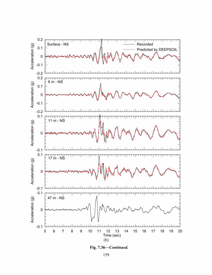
159

-0.2

-0.1

0

0.1

0.2

Acc

eler

atio

n (g

) RecordedPredicted by DEEPSOIL

Surface - NS

-0.2

-0.1

0

0.1

0.2

Acc

eler

atio

n (g

) 6 m - NS

-0.1

0

0.1

Acc

eler

atio

n (g

) 11 m - NS

-0.1

0

0.1

Acc

eler

atio

n (g

) 17 m - NS

5 6 7 8 9 10 11 12 13 14 15 16 17 18 19 20Time (sec)

-0.1

0

0.1

Acc

eler

atio

n (g

) 47 m - NS

(b)

Fig. 7.36—Continued.

160


00.10.20.30.40.50.60.70.80.9

1

Est

imat

ed s

tand

ard

devi

atio

n in

pre

dict

ion

(ln u

nit)

Material Curve variability, σGVelocity variability, σv


Ts = 0.67 sec


spectral ordinates for ground surface. Ts denotes elastic site period.


0.0

0.2

0.4

0.6

Sa (g

)

Downhole record (47 m)Surface Record


-0.8

-0.4

0.0

0.4

0.8

Res

idua

l, R

(ln

units

)

DEEPSOIL with target material curves fromZeghal et al., 1995EPRI, 1993

(a) Surface-EW (b) Surface-NS


Fig. 7.38 Acceleration response spectra for data and simulation results (using DEEPSOIL

with different target material curves) compared through direct spectral ordinates and prediction residuals for ground surface.

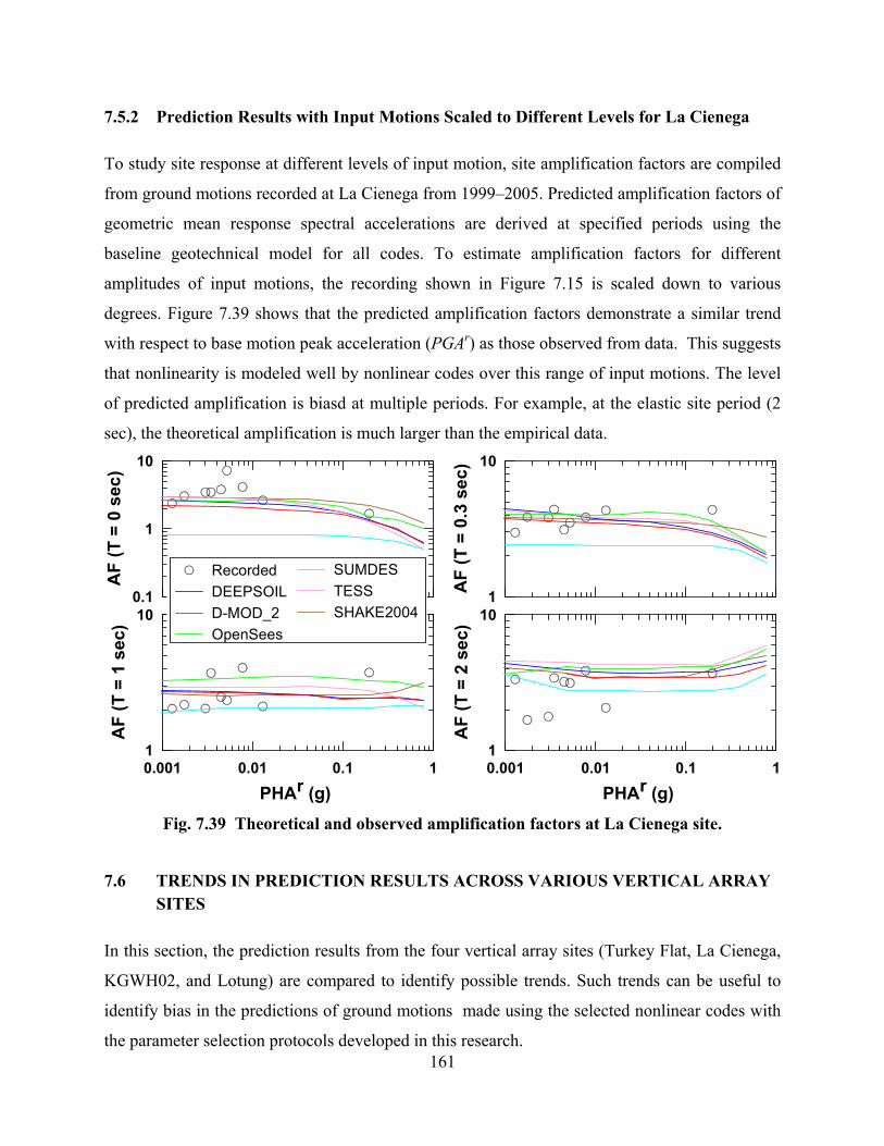
161

7.5.2 Prediction Results with Input Motions Scaled to Different Levels for La Cienega

To study site response at different levels of input motion, site amplification factors are compiled

from ground motions recorded at La Cienega from 1999–2005. Predicted amplification factors of

geometric mean response spectral accelerations are derived at specified periods using the

baseline geotechnical model for all codes. To estimate amplification factors for different

amplitudes of input motions, the recording shown in Figure 7.15 is scaled down to various

degrees. Figure 7.39 shows that the predicted amplification factors demonstrate a similar trend

with respect to base motion peak acceleration (PGAr) as those observed from data. This suggests

that nonlinearity is modeled well by nonlinear codes over this range of input motions. The level

of predicted amplification is biasd at multiple periods. For example, at the elastic site period (2

sec), the theoretical amplification is much larger than the empirical data.

0.1

1

10

AF

(T =

0 s

ec)

1

10A

F (T

= 0

.3 s

ec)

0.001 0.01 0.1 1

PHAr (g)

1

10

AF

(T =

1 s

ec)

0.001 0.01 0.1 1

PHAr (g)

1

10

AF

(T =

2 s

ec)

RecordedDEEPSOILD-MOD_2OpenSees

SUMDESTESSSHAKE2004

Fig. 7.39 Theoretical and observed amplification factors at La Cienega site.

7.6 TRENDS IN PREDICTION RESULTS ACROSS VARIOUS VERTICAL ARRAY SITES

In this section, the prediction results from the four vertical array sites (Turkey Flat, La Cienega,

KGWH02, and Lotung) are compared to identify possible trends. Such trends can be useful to

identify bias in the predictions of ground motions made using the selected nonlinear codes with

the parameter selection protocols developed in this research.

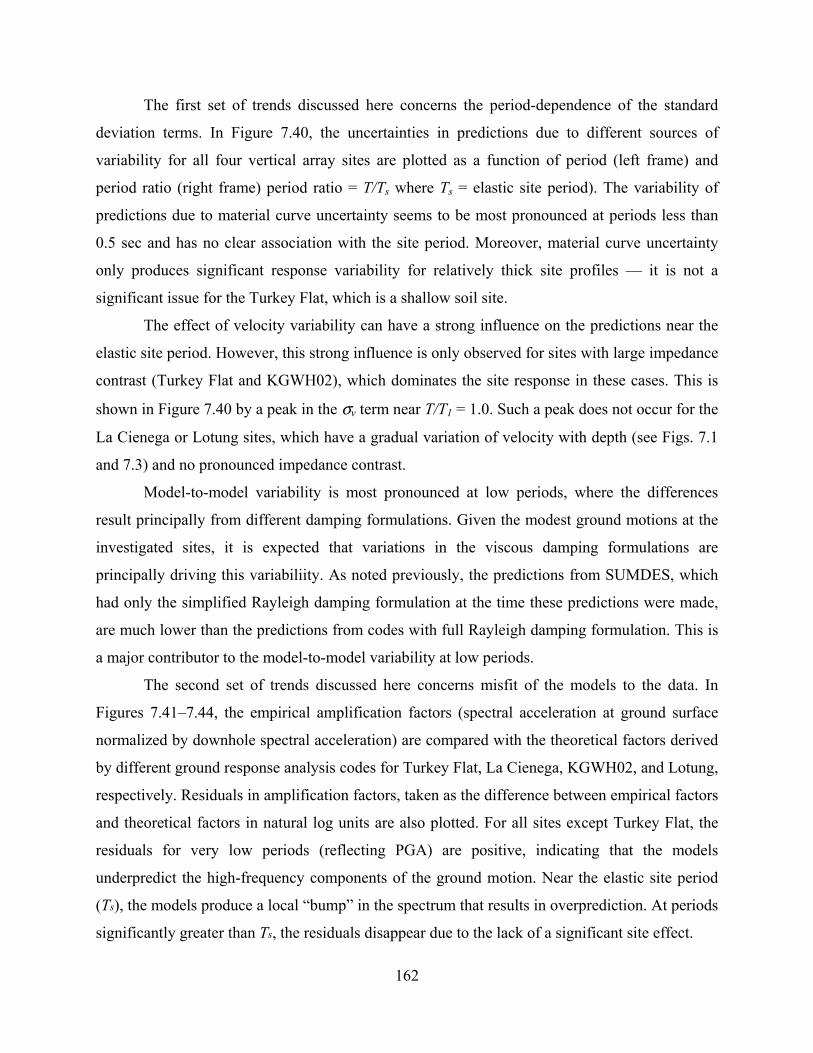
162

The first set of trends discussed here concerns the period-dependence of the standard

deviation terms. In Figure 7.40, the uncertainties in predictions due to different sources of

variability for all four vertical array sites are plotted as a function of period (left frame) and

period ratio (right frame) period ratio = T/Ts where Ts = elastic site period). The variability of

predictions due to material curve uncertainty seems to be most pronounced at periods less than

0.5 sec and has no clear association with the site period. Moreover, material curve uncertainty

only produces significant response variability for relatively thick site profiles — it is not a

significant issue for the Turkey Flat, which is a shallow soil site.

The effect of velocity variability can have a strong influence on the predictions near the

elastic site period. However, this strong influence is only observed for sites with large impedance

contrast (Turkey Flat and KGWH02), which dominates the site response in these cases. This is

shown in Figure 7.40 by a peak in the σv term near T/T1 = 1.0. Such a peak does not occur for the

La Cienega or Lotung sites, which have a gradual variation of velocity with depth (see Figs. 7.1

and 7.3) and no pronounced impedance contrast.

Model-to-model variability is most pronounced at low periods, where the differences

result principally from different damping formulations. Given the modest ground motions at the

investigated sites, it is expected that variations in the viscous damping formulations are

principally driving this variabiliity. As noted previously, the predictions from SUMDES, which

had only the simplified Rayleigh damping formulation at the time these predictions were made,

are much lower than the predictions from codes with full Rayleigh damping formulation. This is

a major contributor to the model-to-model variability at low periods.

The second set of trends discussed here concerns misfit of the models to the data. In

Figures 7.41–7.44, the empirical amplification factors (spectral acceleration at ground surface

normalized by downhole spectral acceleration) are compared with the theoretical factors derived

by different ground response analysis codes for Turkey Flat, La Cienega, KGWH02, and Lotung,

respectively. Residuals in amplification factors, taken as the difference between empirical factors

and theoretical factors in natural log units are also plotted. For all sites except Turkey Flat, the

residuals for very low periods (reflecting PGA) are positive, indicating that the models

underpredict the high-frequency components of the ground motion. Near the elastic site period

(Ts), the models produce a local “bump” in the spectrum that results in overprediction. At periods

significantly greater than Ts, the residuals disappear due to the lack of a significant site effect.

163

The above misfits can have many sources. In general, there are two possible sources of

misfit — error in the input data (velocity profiles or nonlinear curves) or error in the models and

their parameter selection protocols. The errors in the velocity profile were checked by comparing

the observed (small amplitude) shear wave travel time to the time implied by the model. With the

exception of the Kiknet site, these checks confirm the velocity profile used in the analysis. For

KGWH02, the observed travel times are less than the model travel time, which may be due to the

highly 3D nature of the site. Dr. R. Kayen (pers. comm. 2007), who performed the SASW testing

for KGWH02, observed that the site is about 150 m from an outcropping hill and that the

bedrock surface is steep (~30% grade). He suspected that the motions may not be vertically

incident in the rock and may arrive at the site from sloping surface to the west.

Apart from velocity, other possible sources of error include incorrect modeling of

material curves (modulus reduction and damping) or the presence of site response physics that

cannot be captured by a 1D model. Because modulus reduction effects are likely relatively

modest given the low strain levels excited by the subject earthquakes, error in the modeling in

modulus reduction is not likely the source of the misfit. Given that site amplification is

underpredicted for all three sites considered across a broad frequency range, a likely source of

bias is overdamping in the models. This overdamping could reflect bias in the material damping

curves or excessive Rayleigh damping. Further research is needed to resolve these possible

sources of bias.

164

0

0.2

0.4

0.6

0.8

1

Ove

rall

Varia

bilit

y, σ

(ln

uni

t)

0

0.2

0.4

0.6

0.8

1

Mat

eria

l Cur

ve V

aria

bilit

y, σ

G

(ln u

nit)

0

0.2

0.4

0.6

0.8

1

Velo

city

Var

iabi

lity,

σV

(ln u

nit)

0.01 0.1 1 10Period, T (sec)

0

0.2

0.4

0.6

0.8

1

Mod

el V

aria

bilit

y, σ

m

(ln u

nit)

0.001 0.01 0.1 1 10 100Period Ratio, T/Ts

Turkey FlatKiknet KGWH02La CienegaLotung

Fig. 7.40 Comparison of variabilities across three vertical array sites.

165

0

1

2

3

4

5

6

7

AF

DataDEEPSOILD-MOD_2OpenSeesSUMDESTESSSHAKE04


-1

-0.5

0

0.5

1R

esid

ual i

n A

F

Fig. 7.41 Comparison of empirical and theoretical amplification factors across periods for

Turkey Flat site using Parkfield event.


-1.5

-1

-0.5

0

0.5

1

1.5

Res

idua

l in

AF

0

1

2

3

4

5

AF



La Cienega site using 09/09/2001 event.

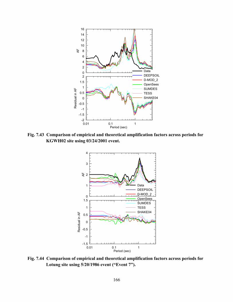
166


-2

-1.5

-1

-0.5

0

0.5

1

1.5

2R

esid

ual i

n A

F0

2

4

6

8

10

12

14

16

AF



KGWH02 site using 03/24/2001 event.


-1.5

-1

-0.5

0

0.5

1

1.5

Res

idua

l in

AF

0

1

2

3

4

AF



Lotung site using 5/20/1986 event (“Event 7”).

167

7.7 COMPARISON OF RESULTS FROM EQUIVALENT-LINEAR AND NONLINEAR ANALYSES

The predictions of ground motions at vertical array sites described in the previous section were

made using both equivalent-linear and nonlinear codes. The aforementioned comparisons of

model predictions to data showed similar trends for both methods of analysis, although the

positive residuals at short periods were generally smaller for equivalent-linear.

More meaningful insight into the differences between equivalent-linear and nonlinear

ground motion predictions can be made when the codes are exercised at relatively strong shaking

levels that induce large strains. Representative results are shown in Figure 4.45, which shows for

the La Cienega site geometric mean horizontal component predicted spectra, amplification

factors (=surface/input outcropping spectral accelerations), and spectral shapes (Sa/PGA) for a

low-strain condition (left side, corresponding to observed motions during the 2001 event) and a

large-strain condition produced through the use of a large amplitude synthetic input motion (right

side). The results shown in Figure 4.45 apply to the baseline geotechnical model described

previously. Also shown for reference purposes are predictions of empirical models for

amplification (middle frames; Choi and Stewart 2005) and spectral shape (bottom frames;

Campbell and Bozorgnia 2007). The empirical amplification model is exercised for a site’s Vs30

(260 m/s) and corresponding input PGA. The empirical spectrum from which the spectral shape

is evaluated is calculated using Mw=7.5, site-source distance=10 km, and strike-slip focal

mechanism (for synthetic). As shown in the bottom frames of Figure 4.45, the spectral shapes

from equivalent-linear and nonlinear models are similar to each other for the 2001 input motion

that induces relatively low strain but are significantly different for the large amplitude synthetic

motion. For the large-strain simulation, the spectral shapes at low periods (< ~0.2 sec) from

equivalent-linear analyses are flatter and have less period-to-period fluctuations than those from

nonlinear analyses or empirical models. This aspect of equivalent-linear results is believed to be

non-physical and can be overcome with nonlinear analysis. As shown in the middle frames, the

flatness of the equivalent-linear spectrum is associated with a dip in the amplification factors

between periods of approximately 0.03–0.3 sec. That dip is less pronounced in the nonlinear

codes, which produce amplification factor shapes more compatible with the empirical model.

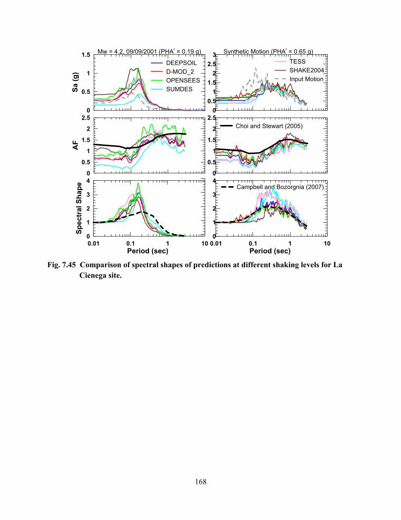
168

0

0.5

1

1.5

Sa (g

)

Mw = 4.2, 09/09/2001 (PHAr = 0.19 g)

DEEPSOILD-MOD_2OPENSEESSUMDES

TESSSHAKE2004Input Motion

00.5

11.5

22.5

3 Synthetic Motion (PHAr = 0.65 g)

0

0.5

1

1.5

2

2.5

AF

Choi and Stewart (2005)

0

0.5

1

1.5

2

2.5

0.01 0.1 1 10Period (sec)

0

1

2

3

4

Spec

tral

Sha

pe Campbell and Bozorgnia (2007)

0.01 0.1 1 10Period (sec)

0

1

2

3

4

Fig. 7.45 Comparison of spectral shapes of predictions at different shaking levels for La

Cienega site.

8 Summary and Conclusions

8.1 SCOPE OF RESEARCH

Ground motion prediction equations are used in seismic hazard analyses to provide a

probabilistic distribution of a particular ground motion intensity measure (IM) conditional on

source, path, and site parameters. The estimates from such relationships only represent averaged

values across the range of possible site conditions within the rock or soil categories, while the

actual site conditions can be influenced by sediment response to upwardly propagating body

waves (ground response effects), basin effects, and surface topography. Ground response effects

can be quantified by site amplification factor models (derived empirically or theoretically) or

site-specific theoretical ground response analyses for which soil material models can be either

equivalent-linear or nonlinear.

Nonlinear ground response analyses are seldom used in engineering practice because they

require the specification of input parameters that lack an obvious association with fundamental

soil properties and because the sensitivity of the site response results to these parameters is not

well understood. Moreover, parameter selection criteria and code usage protocols do not exist or

are poorly documented for many codes, which effectively erect a barrier to code usage for non-

expert users. Key hurdles to practical application of nonlinear ground response analyses were

identified as the selection of parameters describing the backbone curves (which affects both soil

nonlinearity and hysteretic damping), the specification of input motions (“outcropping” versus

“within”), and the specification of viscous damping (i.e., the target value of the viscous damping

ratio and frequencies for which the viscous damping produced by the model matches the target).

Exact (linear frequency-domain) solutions for body-wave propagation through an elastic medium

were used to establish guidelines for the specification of input motions and viscous damping.

Strategies for specifying backbone-curve parameters armed only with basic information on soil

conditions (small-strain shear modulus and target modulus reduction and damping curves as

170

established from information on soil type, overburden stress, PI, etc.) were developed. Because

these curves are only valid for shear strains less than about 0.1–0.3%, additional guidelines were

developed for intelligently extending the curves to approach the shear strength at large strains.

Options are developed for optimally fitting the modulus reduction curve (MR fitting) and for

establishing a simultaneously optimal fit for modulus reduction and material damping (MRD

fitting).

The parameter selection protocols developed for nonlinear ground response analyses are

tested by comparing predictions to data from vertical arrays and looking for trends in the results.

Key issues that would ideally be examined through this validation exercise include assessing the

adequacy of the viscous damping protocols and comparing alternative strategies for specifying

backbone-curve parameters. In addition, the sensitivity of predictions due to different sources of

variability (material properties and modeling schemes) was studied. Finally, targeted analyses

were performed to facilitate comparisons of the performance of equivalent-linear and nonlinear

analyses for different levels of shaking (different strain conditions).

8.2 RESEARCH FINDINGS AND RECOMMENDATIONS

The results of this research can be broadly categorized as follows: (a) parameter selection

protocols for nonlinear ground response analyses and (b) assessment of performance of nonlinear

ground response analyses. The major conclusions from the study are grouped according to these

categories in the subsections that follow.

(a) Parameter Selection Protocols for Nonlinear Ground Response Analyses

Protocols were developed regarding control motion specification, specification of viscous

damping model and parameters, and specification of parameters describing the nonlinear

backbone curve.

Control Motion Specification: Outcropping control motions should be used as-recorded with an

elastic base. Motions recorded at depth should also be used as-recorded but with a rigid base. In

both cases, the motions are specified at the base of the site profile. For within motions, the depth

at which the recording was made should match the depth of the profile base.

171

Specification of Viscous Damping Model and Parameters: When the option of using more

than one target frequency is available (such as the full Rayleigh damping formulation), it should

be applied in lieu of simplified Rayleigh damping because significant bias at high frequencies

can occur with the latter. Target damping ratios should be set to the small-strain material

damping.

The target frequencies should be selected using an iterative process in which the

frequencies are adjusted to optimally match linear frequency-domain and time-domain analyses.

If such iterative analyses are not possible, or as a first guess of frequencies to get such iterative

analyses started, the two target frequencies in a full Rayleigh damping formulation should be set

to the site frequency and five times the site frequency.

The code SUMDES, for which only the simplified Rayleigh damping formulation is

available, should be used with a damping ratio of 1% at 1 Hz (the code assumes that the target

damping ratio is given at 1 Hz). The code TESS does not use viscous damping but does

introduce a parameter VT that affects unload-reload behavior. This parameter can be set equal to

the small-strain damping (in decimal units).

Specification of Backbone Curve Parameters: The selection of backbone curve parameters

begins with the development of an appropriate shear wave velocity (Vs) profile for the site and

the identification of appropriate target nonlinear modulus reduction and damping curves for each

soil layer at the site. The target nonlinear curves can be established from material-specific testing

or, up to strain levels of approximately 0.1–0.3%, from correlation relationships (Darendeli

2001; Zhang et al. 2005). When large strains are expected in portions of a site (i.e., above a

significant impedance contrast for sites subject to strong input motions), the site characterization

should also include the evaluation of dynamic shear strengths in the potentially affected layers.

The procedures to estimate undrained shear strength through stress normalization are well

established (Ladd 1991), but require modification for rate effects (e.g., Sheahan et al. 1996).

In typical ground response analyses, most soil layers are not expected to approach soil

failure. This will generally be the case in profiles with gradual changes in Vs with depth. For sites

with a large impedance contrast, soil failure would likely be confined only to depth intervals

immediately above (i.e., on the softer side of) the impedance contrast. For all layers not

approaching soil failure, target backbone curves can be defined using modulus reduction

relationships without consideration of shear strength. For problems involving moderate to large-

172

strain response, a hybrid representation that accounts for the shape of the modulus reduction

curve at small strains and shear strength at large strain is recommended.

Ultimately it is hoped that procedures for simultaneously matching target modulus

reduction and material damping curves will be implemented in nonlinear codes, but this is not

currently available. At present, users can choose to match the modulus reduction curve only (MR

fitting) or modulus reduction and damping curves simultaneously (MRD fitting). We recommend

the use of both approaches for large-strain problems to bound the solution.

(b) Assessment of Performance of Nonlinear Ground Response Analyses

The limited available validations against vertical array data suggest that the models produce

reasonable results, although there is some indication of overdamping at high frequencies and

overestimation of site amplification at the resonant frequency of the site model. Possible sources

of the high-frequency misfit include potential bias in the velocity profile, material damping

curves, or a viscous damping level that is too high.

The variability of predictions due to material curve uncertainty seems to be most

pronounced at periods less than 0.5 sec and produces significant response variability only for

relatively thick site profiles — it is not a significant issue for shallow sites. The effect of velocity

variability can have a strong influence on the predictions near the elastic site period, but the

effect is observed only for sites with a large impedance contrast that dominates the site response

in these cases. Model-to-model variability is most pronounced at low periods, where the

differences result principally from different damping formulations.

Nonlinearity is modeled well by nonlinear codes (for input motions with PHAr up to 0.2

g; performance of codes above this level is uncertain because no data are available) although the

level of amplification from theoretical analyses and data demonstrate bias at multiple periods as

explained above.

The results of equivalent-linear (EL) and nonlinear (NL) analyses can be compared by

examining predicted trends in amplification factors versus input motion amplitude at various

periods and by examining trends in spectral shape. With respect to the former issue, EL

amplification factors tend to depart from NL factors at input PGAr (peak acceleration on rock)

values above 0.1–0.2 g. In general, the EL factors were larger than the NL factors for large input

motion levels. The EL and NL spectral shapes start to deviate from each other above PHAr of 0.2

173

g. At low periods (T < 0.1 sec), the EL spectral shapes for strong shaking are flatter and have less

period-to-period fluctuations than the NL spectral shapes. The NL codes DMOD_2, DEEPSOIL,

and OpenSees produce generally similar amplification factors and spectral shapes. The results

from these codes can differ from TESS results at high frequencies, mostly as a result of the

different damping formulation in TESS. The SUMDES results tend to be significantly different

from those of other codes for deep sites, which is attributed to the use of the simplified Rayleigh

damping formulation in SUMDES.

8.3 RECOMMENDATIONS FOR FUTURE RESEARCH

This research has identified several issues that should be considered in future work:

1. So far only three vertical array sites have been used to test the effectiveness of the

parameter selection protocols. More validation sites should be tested to see if the

prediction trends and biases identified in this research are also present in other sites. If

they are consistent across sites, future study is needed to investigate how to reduce these

biases. Possible ways may be to consider revising the current protocols for the

specification of damping (both viscous and hysteretic).

2. Empirical amplification factors for the validation sites show significant event-to-event

variability, particularly at high frequencies. Ground response analyses utilizing the

recorded motions for events with high and low residuals should be performed to see if

any of the event-to-event variability can be explained by features of the input motions

(the analyses for amplification factors in this research used a common waveform). Other

factors that should be considered would involve the location of the site relative to the

respective sources, and consideration of possible 2D and 3D site response effects that

may differ from one event to the next.

3. The nonlinear and equivalent-linear codes considered in this work have not been well

validated at large strain levels. The use of centrifuge test data to enable such validations

was considered, but was dissuaded because the experimental configurations do not

correspond to 1D conditions (Elgamal et al. 2005). If this issue can be resolved, either

through improved experiment design or by implementation of the nonlinear soil models

in 2D and 3D codes, it would be very useful to generate validation data sets at large

strains in the centrifuge. These data would be useful to (1) evaluate the relative ability of

174

EL and NL analysis to capture trends in site amplification and spectral shape as shaking

levels increase; (2) demonstrate the importance of matching the true reference strain

(which is based on shear strength) when specifying backbone curves in lieu of MR or

MRD fitting procedures; and (3) evaluate energy dissipation in site response and the

degree to which it is accurately simulated using the combined viscous and hysteretic

damping formulations currently utilized in NL codes.

4. This research is based on the total stress analysis options in the respective nonlinear

codes. A benchmarking exercise related to the pore pressure generation and dissipation

features of nonlinear codes is needed to guide parameter selection for effective stress

analyses. Validation for such cases will be challenging due to the limited number of

vertical array recordings at liquefiable soil sites. As mentioned in (3) above, centrifuge

studies have the potential to provide useful information in this regard. One issue that

would be particularly useful to consider in the validations is the extent to which model

accuracy improves for codes that consider within-cycle contractive and dilative behavior

(i.e., OpenSees) relative to codes that simply degrade the strength and stiffness of the

backbone curve (e.g., DMOD_2 and TESS).

REFERENCES

Anderson, D.G., and Y.K. Tang (1989). “Summary of soil characterization program for the

Lotung large-scale seismic experiment,” Proc. EPRI/NRC/TPC Workshop on Seismic Soil-

Structure Interaction Analysis Techniques Using Data from Lotung, Taiwan, EPRI NP-6154,

Electric Power Research Institute, Palo Alto, Calif., Vol. 1, 4.1–4.20

Andrade, J.E., and R.I. Borja (2006). “Quantifying sensitivity of local site response models to

statistical variations in soil properties,” Acta Geotechnica, 1, 3–14

Assimaki, D. and E. Kausel (2002). “An equivalent linear algorithm with frequency- and

pressure-dependent moduli and damping for the seismic analysis of deep sites,” Soil

Dynamics and Earthquake Engrg., 22(3), 959–965

Baker, J.W. and C.A. Cornell (2003). “Uncertainty specification and propagation for loss

estimation using FOSM methods,” Proceedings, 9th Int. Conf. on Applications of Statistics

and Probability in Civil Engineering (ICASP9), San Francisco, California: Millpress.,

Rotterdam, Netherlands, 8p.

Beresnev, I. A., Wen, K. L. and Yeh Y. T. (1995) “Seismological evidence for nonlinear elastic

ground behavior during large earthquakes,” Soil Dynamics and Earthquake Eng., 14 (2),

103–114.

Borja, R. I., H.Y. Chao, F.J. Montans and C.H. Lin (1999). “Nonlinear ground response at

Lotung LSST site,” J. Geotech. & Geoenv. Eng., ASCE, 125 (3), 187–197.

Borja, R.I. and W.H. Wu (1994). “Vibration of foundations on incompressible soils with no

elastic region,” J. Geotech. Engrg., ASCE, 120(9), 1570–1592.

Campbell, K.W. and Y. Bozorgnia (2007). “Campbell-Bozorgnia NGA ground motion relations

for the geometric mean horizontal component of peak and spectral ground motion

parameters,” PEER Rpt 2007/02, Pacific Earthquake Engineering Research Center,

Richmond, California

Chang, S.W. (1996). “Seismic response of deep stiff soil deposits,” Ph.D. Thesis, Univ. of

California, Berkeley.

Chang, C.-Y., C.M. Mok, M.S. Power, Y.K. Tang, H.T. Tang, and J.C. Stepp (1990).

“Equivalent linear versus nonlinear ground response analyses at Lotung seismic experiment

site,” Proc. 4th U.S. National Conf. Eqk. Engrg., Vol. 1.

176

Chang, S. W., J.D. Bray and R.B. Seed (1996). “Engineering implications of ground motions

from the Northridge earthquake,” Bull. Seism. Soc. Am., 86, S270–S288.

Ching, J., K.A. Porter, and J.L. Beck (2004). “Uncertainty propagation and fFeature selection for

loss estimation in performance-based earthquake engineering,” EERL Report 2004-02,

Earthquake Engineering Research Laboratory, California Institute of Technology, Pasadena,

California.

Chiu, P., D.E. Pradel, A.O.L. Kwok and J.P. Stewart (2008). “Seismic response analyses for the

Silicon Valley Rapid Transit Project,” Proc. 4th Decennial Geotechnical Earthquake

Engineering and Soil Dynamics Conference, ASCE, Sacramento, CA

Choi, Y. and J.P. Stewart (2005). “Nonlinear site amplification as function of 30 m shear wave

velocity,” Earthquake Spectra, 21, 1–30.

Chopra, A.K. (2000). Dynamics of Structures, 2nd Ed., Prentice Hall, Englewood Cliffs, New

Jersey

Clough, G.W., and J. Penzien (1993). Dynamics of Structures, 2nd Ed., McGraw-Hill, New York.

Cramer, C.H. (1995). “Weak-motion observations and modeling for the Turkey Flat, U.S., site-

effects test area near Parkfield, California,” Bull. Seism. Soc. Am., 85 (2), 440–451

Cramer, C.H. and C.R. Real (1992). “A statistical analysis of submitted site-effects predictions

for the weak-motion blind prediction test conducted at the Turkey Flat, USA, site effects test

area near Parkfield, California,” Proceedings, Int. Sym. on the Effects of Surface Geology on

Seismic Motion, v. 2, March 25–27, Odawara, Japan

Dafalias, Y.F. and E.P. Popov (1979). “A model for nonlinearly hardening materials for complex

loading,” Acta Mechanica, 21(3), 173–192

Darendeli, M. (2001). “Development of a new family of normalized modulus reduction and

material damping curves.” Ph.D. Thesis, Dept. of Civil Eng., Univ. of Texas, Austin.

Darragh, R.B. and I.M. Idriss (1997). “A tale of two sites: Gilroy #2 and Treasure Island – Site

response using and equivalent linear technique,” NEHRP Professional Fellowship Report,

EERI, Oakland, CA.

Day, S. M., J. Bielak, D. Dreger, R. Graves, S. Larsen, K.B. Olsen, A. Pitarka, and L. Ramirez-

Guzman (2006). “Numerical simulation of basin effects on long-period ground motion,”

paper 1857, presented at the 8th U.S. National Conference on Earthquake Engineering, 18–

22 April, San Francisco, California

177

Dickenson, S.E. (1994). “The dynamic response of soft and deep cohesive soils during the Loma

Prieta earthquake of October 17, 1989,” Ph.D. Thesis, Univ. of California, Berkeley.

Dobry, R., R.S. Ladd, F.Y. Yokel, R.M. Chung and D. Powell (1982). “Prediction of pore water

pressure buildup and liquefaction of sands during earthquakes by the cyclic strain method,”

National Bureau of Standards Building Science Series 138, National Bureau of Standards and

Technology, Gaithersburg, Md., 150

Dobry, R., W.G. Pierce, R. Dyvik, G.E. Thomas, and R.S. Ladd. (1985). “Pore pressure model

for cyclic straining of sand,” Research Report, Civil Eng. Dept., Rensselaer Polytechnic

Institute, Troy, New York

Electrical Power Research Institute, EPRI (1993). “Guidelines for determining design basis

ground motions,” Rpt. No. EPRI TR-102293, Electrical Power Research Institute, Palo Alto,

CA.

Elgamal, A.W., M. Zeghal, and E. Parra (1996). “Liquefaction of reclaimed island in Kobe,

Japan,” J. Geotech. Eng., 122 (1), 39–49.

Elgamal, A.W., Z. Yang, T. Lai, B.L. Kutter, D.W. Wilson (2005). “Dynamics response of

saturated dense sand in laminated centrifuge container,” J. Geotech. and Geoenvir. Eng.,

ASCE, 131(5), 598–609

Field, E.H. and K.H. Jacob (1993). “Monte-Carlo simulation of the theoretical site response

variability at Turkey Flat, California, given the uncertainty in the geotechnically derived

input parameters,” Earthquake Spectra, 9 (4), 669–701

Finn, W. D. L., K.W. Lee, and G.R. Martin (1977). “An effective stress model for liquefaction,”

J. Geotech. Eng. Div., ASCE, 103 (6), 517–553.

Graves, R. W. (1996). “Simulating seismic wave propagation in 3D elastic media using

staggered-grid finite-differences,” Bull. Seism. Soc. Am., 86, 1091–1106.

Hardin, B.O. and V.P. Drnevich (1972). “Shear modulus and damping in soils: design equations

and curves,” J. of the Soil Mechanics and Foundations Div., ASCE, 98 (SM7), 667–692

Hashash, Y.M.A. and D. Park (2001). “Non-linear one-dimensional seismic ground motion

propagation in the Mississippi embayment,” Eng. Geology, Amsterdam, 62(1–3), 185–206.

Hashash, Y.M.A. and D. Park (2002). “Viscous damping formulation and high frequency motion

propagation in nonlinear site response analysis,” Soil Dynamics and Earthquake Engrg.,

22(7), 611–624.

178

Hudson, M., I.M. Idriss, and M. Beikae (1994). “QUAD4M – A computer program to evaluate

the seismic response of soil structures using finite element procedures and incorporating a

compliant base.” Center for Geotechnical Modeling, Dept. Civil and Envir. Eng., Univ. of

Calif., Davis, CA

Idriss, I.M. (1990). “Response of soft soil sites during earthquakes,” Proc. H. Bolton Seed

Memorial Symposium, J.M. Duncan (ed.), Vol. 2, 273–290.

Idriss, I.M. and J.I. Sun (1992). SHAKE91: A computer program for conducting equivalent

linear seismic response analyses of horizontally layered soil deposits, Center for Geotech.

Modeling, Univ. of Calif., Davis.

Idriss, I.M. (1993). “Assessment of site response analysis procedures,” Report to National

Institute of Standards and Technology, Gaithersburg, Maryland, Dept. of Civil &

Environmental Eng., Univ. of California, Davis.

Idriss, I.M., R. Dobry and R.D. Singh (1978). “Nonlinear behavior of soft clays during cyclic

loading,” J. Geotech. Eng. Div., ASCE, 104 (GT12), 1427–1447

Isenhower, W. M. , and K. H., II Stokoe (1981). “Strain-rate dependent shear modulus of San

Francisco Bay mud,” International Conference on Recent Advances in Geotechnical

Earthquake Eng. and Soil Dynamics; St. Louis, Mo., pp. 597–602.

Ishihara, K. (1986). “Evaluation of soil properties for use in earthquake response analysis,”

Geomechanical Modeling in Eng. Practice, R. Dungar and J.A. Studer, Eds., A.A.Balkema,

Rotterdam, the Netherlands, 241–275

Iwan, W.D. (1967). “On a class of models for the yielding behavior of continuous and composite

systems,” J. of Applied Mechanics, 34 (E3), 612–617

Jacobsen, L.S. (1930). "Steady forced vibrations as influenced by damping." Transactions, ASME,

Vol. 52, No. 15, 169 - 181.

Joyner, W. B. and A.T.F. Chen (1975). “Calculation of nonlinear ground response in

earthquakes,” Bull. Seism. Soc. Am., 65(5), 1315–1336

Kausel, E. and D. Assimaki (2002). “Seismic simulation inelastic soils via frequency-dependent

moduli and damping.” J. of Engrg. Mech., ASCE, 128(1), 34–47.

Kondner, R. L., and J.S. Zelasko (1963). “A hyperbolic stress-strain formulation of sands,” Proc.

of 2nd Pan American Conference on Soil Mechanics and Foundation Engineering, Sao Paulo,

Brasil, 289–324

179

Kramer, S.L. (1996). Geotechnical Earthquake Engineering, Prentice Hall, Englewood Cliffs,

New Jersey

Kramer, S.L. and A.W. Elgamal (2001). “Modeling soil liquefaction hazards for performance-

based earthquake engineering,” PEER Rept 2001/13, Pacific Earthquake Engineering

Research Center, Richmond, California

Kramer, S.L. and S.B. Paulsen (2004). “Practical use of geotechnical site response models,” Proc.

Int. Workshop on Uncertainties in Nonlinear Soil Properties and their Impact on Modeling

Dynamic Soil Response, PEER Center Headquarters, Richmond, CA

Kwok, O.L.A. (2007). “Application of one-dimensional geotechnical modeling for site response

predictions,” PhD. Thesis, Department of Civil and Environmental Engineering, University

of California, Los Angeles

Kwok, O.L.A, and J.P. Stewart (2006). “Application of theoretical 1D amplification factors for

evaluation of seismic site effects,” Bull. Seismol. Soc. Am., 96, no. 4a, 1422–1436

Kwok, O.L.A., J.P. Stewart, Y.M.A. Hashash, N. Matasovic, R.M. Pyke, Z.L. Wang, and Z.

Yang. (2006). “Utilizing nonlinear seismic ground response analysis for Turkey Flat blind

predictions,” Proceedings, 3rd Int. Sym. on the Effects of Surface Geology on Seismic

Motion, August 29 – September 1, Grenoble, France, Paper 50.

Kwok, O.L.A., J.P. Stewart, Y.M.A. Hashash, N. Matasovic, R.M. Pyke, Z.L. Wang, and Z.

Yang (2007). “Use of exact solutions of wave propagation problems to guide implementation

of nonlinear seismic ground response analysis procedures,” J. of Geotech. & Geoenvir. Eng.,

ASCE, 133, no. 11, 1385–1398

Lacy, S. (1986). “Numerical procedures for nonlinear transient analysis of two-phase soil

system,” PhD Thesis, Princeton Univ. Princeton, N.J.

Ladd, C.C. (1991). “Stability evaluation during staged construction: 22nd Terzaghi Lecture,” J.

Geotech. Engr., ASCE, 117 (4), 537–615

Laird, J.P and K.H. Stokoe (1993). “Dynamic properties of remolded and undisturbed soil

sample tests at high confining pressure,” GR93-6, Electric Power Research Institute

Lanzo, G. and M. Vucetic (1999). “Effect of soil plasticity on damping ratio at small cyclic

strains,” Soils and Foundations, 39(4), 131–141.

180

Lee, M. K. W., and W.D.L. Finn (1975). “DESRA-1, Program for the dynamic effective stress

response analysis of soil deposits including liquefaction evaluation,” Soil Mechanics Series

No.36, Department of Civil Eng., University of British Columbia, Vancouver, Canada

Lee, M.K.W. and W.D.L. Finn. (1978). “DESRA-2: Dynamic effective stress response analysis

of soil deposits with energy transmitting boundary including assessment of liquefaction

potential,” Soil Mechanics Series 36, Dept. of Civil Eng., Univ. of British Columbia,

Vancouver, Canada, 60 p

Li, X.S., Z.L. Wangand C.K. Shen (1992). SUMDES: A nonlinear procedure for response

analysis of horizontally-layered sites subjected to multi-directional earthquake loading, Dept.

of Civil Eng., Univ. of Calif., Davis.

Li, X. S., C.K. Shen, and Z.L. Wang (1998). “Fully coupled inelastic site response analysis for

1986 Lotung earthquake,” J. Geotech. & Geoenv. Eng., ASCE, 124 (7), 560–573.

Liu, A.H., J.P. Stewart, N.A. Abrahamson, Y. Moriwaki, Y. (2001). “Equivalent number of

uniform stress cycles for soil liquefaction analysis,” J. Geotech. & Geoenv. Eng., ASCE, 127

(12), 1017–1026.

Lo Presti, D.C.F., Lai, C.G. and I. Puci (2006). “ONDA: Computer code for nonlinear seismic

response analyses of soil deposits.” J. of Geotech. and Geoenvir. Eng., ASCE, 132(2), 223–

236

Lysmer, J., H.B. Seed and P.B. Schnabel (1971). “Influence of base-rock characteristics on

ground response.” Bull. Seism. Soc. Am., 61(5), 1213–1232

Martin, G.R., W.D.L. Finn, and H.B. Seed (1975). “Fundamentals of liquefaction under cyclic

loading,” J. of the Geotech. Eng. Div., ASCE, 101 (5), 423–438

Martin, P. P. (1975). “Non-linear methods for dynamic analysis of ground response,” Ph. D.

Thesis, Univ. of California, Berkeley.

Martin, P.P and H.B. Seed (1978). “ APOLLO, a computer program for the non-linear analysis

of pore pressure generation and dissipation in horizontal sand layers during cyclic earthquake

loading, “ Report No. EERC 78-21, Earthquake Eng. Research Center, Univ. of Calif.,

Berkeley , California

Masing, G. (1926). “Eigenspannungen and verfertigung beim messing.” Proc. 2nd Int. Congress

on Applied Mech., Zurich, Switzerland

181

Matasovic, N. (2006). “D-MOD_2 – A Computer Program for Seismic Response Analysis of

Horizontally Layered Soil Deposits, Earthfill Dams, and Solid Waste Landfills.” User’s

Manual, GeoMotions, LLC, Lacey, Washington, 20 p. (plus Appendices).

Matasovic, N., Kavazanjian, E., Jr. and Abourjeily, F. (1995), “Dynamic Properties of Solid

Waste from Field Observations,” Proc. 1st International Conference on Earthquake

Geotechnical Engineering, Tokyo, Japan, Vol. 1,pp. 549-554.

Matasovic, N. and M. Vucetic (1993a). “Cyclic Characterization of Liquefiable Sands,” J. of

Geotech. Eng., ASCE, 119(11), 1805-1822

Matasovic, N. and M. Vucetic (1993b). “Seismic response of horizontally layered soil deposits,”

Report No. ENG 93-182, School of Engineering and Applied Science, University of

California, Los Angeles.

Matasovic, N. and M. Vucetic (1995). “Generalized cyclic degradation-pore pressure generation

model for clays,” J. Geotech. Eng., ASCE, 121 (1), 33-42.

Matasovic, J. and M. Vucetic (1996). “Analysis of seismic records from the Wildlife

Liquefaction site,” Proc. 11th World Conf. Earthquake Eng., Disc 1, Paper 209.

McKenna, F. and G.L. Fenves (2001). “The OpenSees command language manual, version 1.2.”

Pacific Earthquake Engrg. Research Center, Univ. of Calif., Berkeley.

(http://opensees.berkeley.edu).

Melchers, R.E. (1999). Structural Reliability Analysis and Prediction. John Wiley and Sons,

Chichester.

Mroz, Z. (1967). “On the description of anisotropic work hardening,” J. Mech. And Physics of

Solids, 15, 163-175

Newmark, N.M. (1959). “A method of computation for structural dynamics,” J. Eng Mech. Div.,

ASCE, 67-94

Nigbor, R. and T. Imai (1994). “The Suspension P-S Velocity Logging Method,” in Geophysical

Characterization of Sites, ISSMFE Special Publication TC 10.

Olsen, K.B. (2000). “Site amplification in the Los Angeles basin from three-dimensional

modeling of ground motion,” Bull. Seism. Soc. Am., 90, S77-S94.

Park, D. and Y.M.A. Hashash (2004). “Soil damping formulation in nonlinear time domain site

response analysis,” J. of Earthquake Eng., 8(2), 249-274.

182

Parra, E. (1996). “Numerical modeling of liquefaction and lateral ground deformation including

cyclic mobility and dilation response in soil systems” PhD Thesis, Dept. of Civil Engrg.,

Rensselaer Polytechnic Institute, Troy, NY.

Pestana, J.M. and F. Nadim (2000). “Nonlinear site response analysis of submerged slopes,”

Report No. UCB/GT/2000-04, Dept. of Civil & Envir. Eng., U.C. Berkeley.

Potts, D.M. and L. Zdravković (1999). Finite element analysis in geotechnical engineering:

theory, Thomas Telford Ltd., London

Prevost, J.H. (1977). “Mathematical modeling of monotonic and cyclic undrained clay

behavior,” Int. J. Numerical and Analytical Methods in Geomechanics, 1 (2), 195-216

Prevost, J.H. (1985). “A simple plasticity theory for frictional cohesionless soils,” Soil Dyn.

Earthquake Eng., 4(1), 9-17

Prevost, J.H. (1989). “DYNA1D - A computer program for nonlinear seismic site response

analysis: Technical documentation,” Rpt. No. NCEER-89-0025, National Center for

Earthquake Engineering Research, Buffalo, N.Y.

Pyke, R.M. (1979). “Nonlinear soil models for irregular cyclic loadings,” J. Geotech. Eng.,

ASCE, 105(GT6), 715-726.

Pyke, R.M. (2000). TESS: A computer program for nonlinear ground response analyses. TAGA

Engineering Systems & Software, Lafayette, Calif.

Qiu, P. (1997). “Earthquake induced nonlinear ground deformation analyses,” Ph.D. Thesis,

Univ. of Southern California.

Ragheb, A. M. (1994).”Numerical analysis of seismically induced deformations in saturated

granular soil strata,” PhD Thesis, Dept. of Civil Eng., Rensselaer Polytechnic Institute, Troy,

NY.

Ramberg, W. and W.R. Osgood (1943) “Description of stress-strain curves by three parameters,”

Technical Note 902, National Advisory Committee for Aeronautics, Washington, D.C.

Rayleigh, J.W.S and R.B. Lindsay (1945). The theory of sound, Dover Publications, New York

Real, C.R. (1988). “Turkey Flat, USA site effects test area – report 2, site characterization,” TR

88-2, Calif. Div. of Mines and Geology

Real, C.R. and C.H. Cramer. (1989) “Turkey Flat, USA Site Effects Test Area – report 3: weak-

motion test: prediction criteria and input rock motions,” TR 89-1, Calif. Div. of Mines and

Geology

183

Real, C.R. and A.F. Shakal. (2005). “Turkey Flat, USA site effects test area - report 7, strong

motion test: prediction criteria and data formats,” CSMIP Rept. OSMS 05-01, Calif.

Geological Survey, Dept. of Conservation.

Real, C.R., A.F. Shakal, B.E. Tucker (2006). “Turkey Flat, U.S.A. site effects test area: anatomy

of a blind ground-motion prediction test,” Proceedings, 3rd Int. Sym. on the Effects of

Surface Geology on Seismic Motion, August 29 e.g., September 1, Grenoble, France, Paper

KN 3.

Roblee, C.J., W.J. Silva, G.R. Toro and N.A. Abrahamson (1996). “Variability in site-specific

seismic ground motion design predictions,” ASCE Geotech. Special Publication No. 58,

Uncertainty in the Geologic Environment: From Theory to Practice, C.D. Shakelford, P.P.

Nelson (eds.), Vol. 2, 1113-1133

Roesset, J.M. and R.V. Whitman (1969). “Theoretical background for amplification studies.”

Research report R69-15, Soils publications no. 231, Massachusetts Institute of Technology,

Cambridge, Massachusetts

Roscoe, K.H. and J.B. Burland (1968). “On the generalized stress-strain behavior of ‘wet’ clay,”

J. Heyman and F.A. Leckie, eds., Eng. Plasticity, University Press, Cambridge, 535-609

Roscoe, K.H. and A.N. Schofield (1963). “Mechanical behavior of an idealized ‘wet’ clay,” Proc.

of 2nd European Conference on Soil Mechanics, Wiesbaden, Germany, Vol. 1, 47-54

Rosenblueth, E., 1975, “Point estimates for probability moments,” Proc. Nat. Acad. of Sci.,

72(10), 3812-3814

ROSRINE, Resolution of Site Response Issues from the Northridge Earthquake,

http://gees.usc.edy/ROSRINE

Rymer, M.J., J.C. Tinsley III, J.A. Treiman, J.R. Arrowsmith, K.B. Clahan, A.M. Rosinski, W.A.

Bryant, H.A. Snyder, G.S. Fuis, N.A. Toke and G.W. Bawden (2006). “Surface fault slip

associated with the 2004 Parkfield, California, earthquake,” Bull. Seism. Soc. Am., 96 (4B),

S11-S27

Schnabel, P.B, J. Lysmer and H.B. Seed (1972). “SHAKE: A computer program for earthquake

response analysis of horizontally layered site,.” Report no. UCB/EERC-72/12, Earthquake

Engrg. Research Center, Univ. of Calif., Berkeley, California, 102p

Seed, H.B. (1979). “Soil liquefaction and cyclic mobility evaluation for level ground during

earthquake,” J. Geotech. Engr. Div., ASCE, 105, GT2, 201-225

184

Seed, H.B. and I.M. Idriss (1970). “Soil moduli and damping factors for dynamic response

analyses,” Report EERC 70-10, Earthquake Engineering Research Center, University of

California, Berkeley.

Seed, H.B., I.M. Idriss, F. Makdisi, and N. Banerjee (1975) “Representation of irregular stress

time histories by equivalent uniform stress series in liquefaction analyses,” Rpt EERC 75-29,

Earthquake Engineering Research Center, Univ. of California, Berkeley.

Seed, H.B., P.P. Martin and J. Lysmer (1976) “Pore-water pressure changes during soil

liquefaction, ”J. Geotech. Eng. Div., ASCE, 102 (GT4), 323-346

Seed, H.B., M.P. Romo, J.I. Sun, A. Jaime and J. Lysmer (1987). “Relationships between soil

conditions and earthquake ground motions in Mexico City in the earthquake of September

19, 1985,” Rpt. No. UCB/EERC-87/15, Earthquake Eng. Research Center, Univ. of Calif.,

Berkeley.

Seed, H.B., R.T. Wong, I.M. Idriss and K. Tokimatsu (1984). “Moduli and damping factors for

dynamic analyses of cohesionless soils,” Rpt UCB/EERC-84/14, Earthquake Engineering

Research Center, Univ. of California, Berkeley, Calif.

Sheahan, T.C., C.C. Ladd, and J.T. Germaine (1996) “Rate-dependent undrained shear behavior

of saturated clay,” J. Geotech. Engr., ASCE, 122 (2), 99-108

Silva, W.J., N. Abrahamson, G. Toro, C. Costantino (1996) “Description and validation of the

stochastic ground motion model,” Research report prepared for the Engineering Research and

Applications Division, Department of Nuclear Energy, Brookhaven National Laboratory,

Associated Universities, New York

Silva, W.J. and K. Lee (1987). “WES RASCAL code for synthesizing earthquake ground

motions,” State of the Art for Assessing Earthquake Hazards in the United States, Report 24,

U.S. Army Engineers Waterway Experiment Station, Misc. Paper S-73-1.

Silva, W.J., R.B. Darragh, N. Gregor, G. Martin, N.A. Abrahamson, and C. Kircher (2000).

“Reassessment of site coefficients and near-fault factors for building code provisions,”

Report to U.S. Geological Survey, National Earthquake Hazards Reduction Program.

Stewart, J.P., O.L.A. Kwok, Y.M.A. Hashash, N. Matasovic, R. Pyke, Z.L. Wang, and Z. Yang

(2006). “Overcoming hurdles that limit the application of nonlinear seismic ground response

analysis in engineering practice,” 5th National Seismic Conference on Bridges and Highways,

San Francisco, CA

185

Stewart, J.P. and O.L.A. Kwok (2008). “Nonlinear seismic ground response analysis: code usage

protocols and verification against vertical array data,” Proc. 4th Decennial Geotechnical

Earthquake Engineering and Soil Dynamics Conference, ASCE, Sacramento, CA

Sun, J.I., R. Golesorkhi, and H.B. Seed (1988). “Dynamic moduli and damping ratios for

cohesive soils,” Rpt UCB/EERC-88/15, Earthquake Engineering Research Center, Univ. of

California, Berkeley, Calif.

Tan, K. and M. Vucetic (1989). “Behavior of medium and low plasticity clays under cyclic

simple shear conditions,” Proc. 4th International Conference on Soil Dynamics and

Earthquake Engineering, Soil Dynamics and Liquefaction Volume, Mexico City, 131-142

Terzaghi, K. (1925). Erdbaumechanik auf Bodenphysikalischer Grundlage, Franz Deuticke,

Leipzig und Wein

Toro, G. R. (1997). ‘‘Probabilistic models of shear-wave velocity profiles at the Savannah River

site, South Carolina.’’ Rep. to Pacific Engineering and Analysis, El Cerrito, Calif.

Tucker, B.E. and C.R. Real (1986). “Turkey Flat, USA site effects test area – report 1: needs,

goals, and objectives,” TR 86-1, Calif. Div. of Mines and Geology

Vucetic, M. (1990). “Normalized behavior of clay under irregular cyclic loading.” Canadian

Geotech. J., 27, 29-46.

Vucetic, M. (1994). “Cyclic characterization for seismic regions based on PI,” Proc. XIII

International (World) Conference on Soil Mechanics and Foundation Engineering, New

Delhi, India, Vol 1, 329-332

Vucetic, M. and R. Dobry (1986). “Pore pressure buildup and liquefaction at level sandy sites

during earthquakes,” Research report CE-86-3, Dept. Civil Eng., Rensselaer Polytechnic

Institute, New York

Vucetic, M. and R. Dobry (1988). “Degradation of marine clays under cyclic loading,” J. of the

Geotech. Eng., ASCE, 114 (2), 133-149

Vucetic, M. and R. Dobry (1991). “Effect of soil plasticity on cyclic response,” J. Geotech. Eng.,

117, 89-107.

Vucetic, M., G. Lanzo, and M. Doroudian (1998). “Damping at small strains in cyclic simple

shear test.” J. Geotech. and Geoenviron. Eng., ASCE, 124(7), 585-594.

186

Wang, Z.L. (1990). “Bounding surface hypoplasticity model for granular soils and its

applications.” PhD. Thesis, Univ. of Calif., Davis

Wang, Z.L., Y.F. Dafalias, C.K. Shen (1990). “Bounding surface hypoplasticity model for sand,”

J. Eng. Mech., ASCE, 116 (5)

Wang, Z.L., Q.Y. Han, and G.S. Zhou (1980). “Wave propagation method of site seismic

response by visco-elastoplastic model,” Proc. of Seventh World Conf. on Earthquake Eng.,

V2, 379-386

Wang, Z.L., C.-Y. Chang, and C.M. Mok (2001). “Evaluation of site response using downhole

array data from a liquefied site,” Proc. 4th Int. Conf. Recent Advances in Geotech. Eqk. Eng.

Soil Dyn., Paper 4.30.

Weiler, W.A. (1988). “Small strain shear modulus of clay,” Proc. of ASCE Conference on

Earthquake Engineering and Soil Dynamics II: Recent Advances in Ground Motion

Evaluation, Geotechnical Special Publication 20, ASCE, New York, 331-345.

Wilson, E.L. (1968). “A computer program for the dynamic stress analysis of underground

structures,” EERC Rpt 76-29, Earthquake Eng. Research Center, Univ. of California,

Berkeley

Yang, Z. (2000). “Numerical modeling of earthquake site response including dilation and

liquefaction,” PhD Thesis, Dept. of Civil Eng. and Eng. Mech., Columbia University, NY,

New York

Yang, Z., A. Elgamal and E. Parra (2003). “Computational model for cyclic mobility and

associated shear deformation,” J. Geotech. and Geoenvir. Eng., ASCE, 129(12), 1119-1127.

Youngs, R.R. (2004). Software validation report for SHAKE04, Geomatrix Consultants

Zhang, J., R.D. Andrus and C.H. Juang (2005) “Normalized shear modulus and material

damping ratio relationships,” J. Geotech. and Geoenvir. Eng., ASCE, 131(4), 453-464.

Zeghal M., A.W. Elgamal, H.T. Tang, and J.C. Stepp (1995). “Lotung downhole array II:

evaluation of soil nonlinear properties,” J. Geotech. Engr., 121(4), 363-378

PEER REPORTS

PEER reports are available from the National Information Service for Earthquake Engineering (NISEE). To order PEER reports, please contact the Pacific Earthquake Engineering Research Center, 1301 South 46th Street, Richmond, California 94804-4698. Tel.: (510) 665-3405; Fax: (510) 665-3420.

PEER 2008/05 Performance-Based Earthquake Engineering Design Evaluation Procedure for Bridge Foundations Undergoing Liquefaction-Induced Lateral Ground Displacement. Christian A. Ledezma and Jonathan D. Bray. August 2008.

PEER 2008/04 Benchmarking of Nonlinear Geotechnical Ground Response Analysis Procedures. Jonathan P. Stewart, Annie On-Lei Kwok, Youssef M. A. Hashash, Neven Matasovic, Robert Pyke, Zhiliang Wang, and Zhaohui Yang. August 2008.

PEER 2008/03 Guidelines for Nonlinear Analysis of Bridge Structures in California. Ady Aviram, Kevin R. Mackie, and Božidar Stojadinović. August 2008.

PEER 2008/02 Treatment of Uncertainties in Seismic-Risk Analysis of Transportation Systems. Evangelos Stergiou and Anne S. Kiremidjian. July 2008.

PEER 2008/01 Seismic Performance Objectives for Tall Buildings. William T. Holmes, Charles Kircher, William Petak, and Nabih Youssef. August 2008.

PEER 2007/12 An Assessment to Benchmark the Seismic Performance of a Code-Conforming Reinforced Concrete Moment-Frame Building. Curt Haselton, Christine A. Goulet, Judith Mitrani-Reiser, James L. Beck, Gregory G. Deierlein, Keith A. Porter, Jonathan P. Stewart, and Ertugrul Taciroglu. August 2008.

PEER 2007/11 Bar Buckling in Reinforced Concrete Bridge Columns. Wayne A. Brown, Dawn E. Lehman, and John F. Stanton. February 2008.

PEER 2007/10 Computational Modeling of Progressive Collapse in Reinforced Concrete Frame Structures. Mohamed M. Talaat and Khalid M. Mosalam. May 2008.

PEER 2007/09 Integrated Probabilistic Performance-Based Evaluation of Benchmark Reinforced Concrete Bridges. Kevin R. Mackie, John-Michael Wong, and Božidar Stojadinović. January 2008.

PEER 2007/08 Assessing Seismic Collapse Safety of Modern Reinforced Concrete Moment-Frame Buildings. Curt B. Haselton and Gregory G. Deierlein. February 2008.

PEER 2007/07 Performance Modeling Strategies for Modern Reinforced Concrete Bridge Columns. Michael P. Berry and Marc O. Eberhard. April 2008.

PEER 2007/06 Development of Improved Procedures for Seismic Design of Buried and Partially Buried Structures. Linda Al Atik and Nicholas Sitar. June 2007.

PEER 2007/05 Uncertainty and Correlation in Seismic Risk Assessment of Transportation Systems. Renee G. Lee and Anne S. Kiremidjian. July 2007.

PEER 2007/04 Numerical Models for Analysis and Performance-Based Design of Shallow Foundations Subjected to Seismic Loading. Sivapalan Gajan, Tara C. Hutchinson, Bruce L. Kutter, Prishati Raychowdhury, José A. Ugalde, and Jonathan P. Stewart. May 2008.

PEER 2007/03 Beam-Column Element Model Calibrated for Predicting Flexural Response Leading to Global Collapse of RC Frame Buildings. Curt B. Haselton, Abbie B. Liel, Sarah Taylor Lange, and Gregory g. Deierlein. May 2008.

PEER 2007/02 Campbell-Bozorgnia NGA Ground Motion Relations for the Geometric Mean Horizontal Component of Peak and Spectral Ground Motion Parameters. Kenneth W. Campbell and Yousef Bozorgnia. May 2007.

PEER 2007/01 Boore-Atkinson NGA Ground Motion Relations for the Geometric Mean Horizontal Component of Peak and Spectral Ground Motion Parameters. David M. Boore and Gail M. Atkinson. May. May 2007.

PEER 2006/12 Societal Implications of Performance-Based Earthquake Engineering. Peter J. May. May 2007.

PEER 2006/11 Probabilistic Seismic Demand Analysis Using Advanced Ground Motion Intensity Measures, Attenuation Relationships, and Near-Fault Effects. Polsak Tothong and C. Allin Cornell. March 2007.

PEER 2006/10 Application of the PEER PBEE Methodology to the I-880 Viaduct. Sashi Kunnath. February 2007.

PEER 2006/09 Quantifying Economic Losses from Travel Forgone Following a Large Metropolitan Earthquake. James Moore, Sungbin Cho, Yue Yue Fan, and Stuart Werner. November 2006.

PEER 2006/08 Vector-Valued Ground Motion Intensity Measures for Probabilistic Seismic Demand Analysis. Jack W. Baker and C. Allin Cornell. October 2006.

PEER 2006/07 Analytical Modeling of Reinforced Concrete Walls for Predicting Flexural and Coupled–Shear- Flexural Responses. Kutay Orakcal, Loenardo M. Massone, and John W. Wallace. October 2006.

PEER 2006/06 Nonlinear Analysis of a Soil-Drilled Pier System under Static and Dynamic Axial Loading. Gang Wang and Nicholas Sitar. November 2006.

PEER 2006/05 Advanced Seismic Assessment Guidelines. Paolo Bazzurro, C. Allin Cornell, Charles Menun, Maziar Motahari, and Nicolas Luco. September 2006.

PEER 2006/04 Probabilistic Seismic Evaluation of Reinforced Concrete Structural Components and Systems. Tae Hyung Lee and Khalid M. Mosalam. August 2006.

PEER 2006/03 Performance of Lifelines Subjected to Lateral Spreading. Scott A. Ashford and Teerawut Juirnarongrit. July 2006.

PEER 2006/02 Pacific Earthquake Engineering Research Center Highway Demonstration Project. Anne Kiremidjian, James Moore, Yue Yue Fan, Nesrin Basoz, Ozgur Yazali, and Meredith Williams. April 2006.

PEER 2006/01 Bracing Berkeley. A Guide to Seismic Safety on the UC Berkeley Campus. Mary C. Comerio, Stephen Tobriner, and Ariane Fehrenkamp. January 2006.

PEER 2005/16 Seismic Response and Reliability of Electrical Substation Equipment and Systems. Junho Song, Armen Der Kiureghian, and Jerome L. Sackman. April 2006.

PEER 2005/15 CPT-Based Probabilistic Assessment of Seismic Soil Liquefaction Initiation. R. E. S. Moss, R. B. Seed, R. E. Kayen, J. P. Stewart, and A. Der Kiureghian. April 2006.

PEER 2005/14 Workshop on Modeling of Nonlinear Cyclic Load-Deformation Behavior of Shallow Foundations. Bruce L. Kutter, Geoffrey Martin, Tara Hutchinson, Chad Harden, Sivapalan Gajan, and Justin Phalen. March 2006.

PEER 2005/13 Stochastic Characterization and Decision Bases under Time-Dependent Aftershock Risk in Performance-Based Earthquake Engineering. Gee Liek Yeo and C. Allin Cornell. July 2005.

PEER 2005/12 PEER Testbed Study on a Laboratory Building: Exercising Seismic Performance Assessment. Mary C. Comerio, editor. November 2005.

PEER 2005/11 Van Nuys Hotel Building Testbed Report: Exercising Seismic Performance Assessment. Helmut Krawinkler, editor. October 2005.

PEER 2005/10 First NEES/E-Defense Workshop on Collapse Simulation of Reinforced Concrete Building Structures. September 2005.

PEER 2005/09 Test Applications of Advanced Seismic Assessment Guidelines. Joe Maffei, Karl Telleen, Danya Mohr, William Holmes, and Yuki Nakayama. August 2006.

PEER 2005/08 Damage Accumulation in Lightly Confined Reinforced Concrete Bridge Columns. R. Tyler Ranf, Jared M. Nelson, Zach Price, Marc O. Eberhard, and John F. Stanton. April 2006.

PEER 2005/07 Experimental and Analytical Studies on the Seismic Response of Freestanding and Anchored Laboratory Equipment. Dimitrios Konstantinidis and Nicos Makris. January 2005.

PEER 2005/06 Global Collapse of Frame Structures under Seismic Excitations. Luis F. Ibarra and Helmut Krawinkler. September 2005.

PEER 2005//05 Performance Characterization of Bench- and Shelf-Mounted Equipment. Samit Ray Chaudhuri and Tara C. Hutchinson. May 2006.

PEER 2005/04 Numerical Modeling of the Nonlinear Cyclic Response of Shallow Foundations. Chad Harden, Tara Hutchinson, Geoffrey R. Martin, and Bruce L. Kutter. August 2005.

PEER 2005/03 A Taxonomy of Building Components for Performance-Based Earthquake Engineering. Keith A. Porter. September 2005.

PEER 2005/02 Fragility Basis for California Highway Overpass Bridge Seismic Decision Making. Kevin R. Mackie and Božidar Stojadinović. June 2005.

PEER 2005/01 Empirical Characterization of Site Conditions on Strong Ground Motion. Jonathan P. Stewart, Yoojoong Choi, and Robert W. Graves. June 2005.

PEER 2004/09 Electrical Substation Equipment Interaction: Experimental Rigid Conductor Studies. Christopher Stearns and André Filiatrault. February 2005.

PEER 2004/08 Seismic Qualification and Fragility Testing of Line Break 550-kV Disconnect Switches. Shakhzod M. Takhirov, Gregory L. Fenves, and Eric Fujisaki. January 2005.

PEER 2004/07 Ground Motions for Earthquake Simulator Qualification of Electrical Substation Equipment. Shakhzod M. Takhirov, Gregory L. Fenves, Eric Fujisaki, and Don Clyde. January 2005.

PEER 2004/06 Performance-Based Regulation and Regulatory Regimes. Peter J. May and Chris Koski. September 2004.

PEER 2004/05 Performance-Based Seismic Design Concepts and Implementation: Proceedings of an International Workshop. Peter Fajfar and Helmut Krawinkler, editors. September 2004.

PEER 2004/04 Seismic Performance of an Instrumented Tilt-up Wall Building. James C. Anderson and Vitelmo V. Bertero. July 2004.

PEER 2004/03 Evaluation and Application of Concrete Tilt-up Assessment Methodologies. Timothy Graf and James O. Malley. October 2004.

PEER 2004/02 Analytical Investigations of New Methods for Reducing Residual Displacements of Reinforced Concrete Bridge Columns. Junichi Sakai and Stephen A. Mahin. August 2004.

PEER 2004/01 Seismic Performance of Masonry Buildings and Design Implications. Kerri Anne Taeko Tokoro, James C. Anderson, and Vitelmo V. Bertero. February 2004.

PEER 2003/18 Performance Models for Flexural Damage in Reinforced Concrete Columns. Michael Berry and Marc Eberhard. August 2003.

PEER 2003/17 Predicting Earthquake Damage in Older Reinforced Concrete Beam-Column Joints. Catherine Pagni and Laura Lowes. October 2004.

PEER 2003/16 Seismic Demands for Performance-Based Design of Bridges. Kevin Mackie and Božidar Stojadinović. August 2003.

PEER 2003/15 Seismic Demands for Nondeteriorating Frame Structures and Their Dependence on Ground Motions. Ricardo Antonio Medina and Helmut Krawinkler. May 2004.

PEER 2003/14 Finite Element Reliability and Sensitivity Methods for Performance-Based Earthquake Engineering. Terje Haukaas and Armen Der Kiureghian. April 2004.

PEER 2003/13 Effects of Connection Hysteretic Degradation on the Seismic Behavior of Steel Moment-Resisting Frames. Janise E. Rodgers and Stephen A. Mahin. March 2004.

PEER 2003/12 Implementation Manual for the Seismic Protection of Laboratory Contents: Format and Case Studies. William T. Holmes and Mary C. Comerio. October 2003.

PEER 2003/11 Fifth U.S.-Japan Workshop on Performance-Based Earthquake Engineering Methodology for Reinforced Concrete Building Structures. February 2004.

PEER 2003/10 A Beam-Column Joint Model for Simulating the Earthquake Response of Reinforced Concrete Frames. Laura N. Lowes, Nilanjan Mitra, and Arash Altoontash. February 2004.

PEER 2003/09 Sequencing Repairs after an Earthquake: An Economic Approach. Marco Casari and Simon J. Wilkie. April 2004.

PEER 2003/08 A Technical Framework for Probability-Based Demand and Capacity Factor Design (DCFD) Seismic Formats. Fatemeh Jalayer and C. Allin Cornell. November 2003.

PEER 2003/07 Uncertainty Specification and Propagation for Loss Estimation Using FOSM Methods. Jack W. Baker and C. Allin Cornell. September 2003.

PEER 2003/06 Performance of Circular Reinforced Concrete Bridge Columns under Bidirectional Earthquake Loading. Mahmoud M. Hachem, Stephen A. Mahin, and Jack P. Moehle. February 2003.

PEER 2003/05 Response Assessment for Building-Specific Loss Estimation. Eduardo Miranda and Shahram Taghavi. September 2003.

PEER 2003/04 Experimental Assessment of Columns with Short Lap Splices Subjected to Cyclic Loads. Murat Melek, John W. Wallace, and Joel Conte. April 2003.

PEER 2003/03 Probabilistic Response Assessment for Building-Specific Loss Estimation. Eduardo Miranda and Hesameddin Aslani. September 2003.

PEER 2003/02 Software Framework for Collaborative Development of Nonlinear Dynamic Analysis Program. Jun Peng and Kincho H. Law. September 2003.

PEER 2003/01 Shake Table Tests and Analytical Studies on the Gravity Load Collapse of Reinforced Concrete Frames. Kenneth John Elwood and Jack P. Moehle. November 2003.

PEER 2002/24 Performance of Beam to Column Bridge Joints Subjected to a Large Velocity Pulse. Natalie Gibson, André Filiatrault, and Scott A. Ashford. April 2002.

PEER 2002/23 Effects of Large Velocity Pulses on Reinforced Concrete Bridge Columns. Greg L. Orozco and Scott A. Ashford. April 2002.

PEER 2002/22 Characterization of Large Velocity Pulses for Laboratory Testing. Kenneth E. Cox and Scott A. Ashford. April 2002.

PEER 2002/21 Fourth U.S.-Japan Workshop on Performance-Based Earthquake Engineering Methodology for Reinforced Concrete Building Structures. December 2002.

PEER 2002/20 Barriers to Adoption and Implementation of PBEE Innovations. Peter J. May. August 2002.

PEER 2002/19 Economic-Engineered Integrated Models for Earthquakes: Socioeconomic Impacts. Peter Gordon, James E. Moore II, and Harry W. Richardson. July 2002.

PEER 2002/18 Assessment of Reinforced Concrete Building Exterior Joints with Substandard Details. Chris P. Pantelides, Jon Hansen, Justin Nadauld, and Lawrence D. Reaveley. May 2002.

PEER 2002/17 Structural Characterization and Seismic Response Analysis of a Highway Overcrossing Equipped with Elastomeric Bearings and Fluid Dampers: A Case Study. Nicos Makris and Jian Zhang. November 2002.

PEER 2002/16 Estimation of Uncertainty in Geotechnical Properties for Performance-Based Earthquake Engineering. Allen L. Jones, Steven L. Kramer, and Pedro Arduino. December 2002.

PEER 2002/15 Seismic Behavior of Bridge Columns Subjected to Various Loading Patterns. Asadollah Esmaeily-Gh. and Yan Xiao. December 2002.

PEER 2002/14 Inelastic Seismic Response of Extended Pile Shaft Supported Bridge Structures. T.C. Hutchinson, R.W. Boulanger, Y.H. Chai, and I.M. Idriss. December 2002.

PEER 2002/13 Probabilistic Models and Fragility Estimates for Bridge Components and Systems. Paolo Gardoni, Armen Der Kiureghian, and Khalid M. Mosalam. June 2002.

PEER 2002/12 Effects of Fault Dip and Slip Rake on Near-Source Ground Motions: Why Chi-Chi Was a Relatively Mild M7.6 Earthquake. Brad T. Aagaard, John F. Hall, and Thomas H. Heaton. December 2002.

PEER 2002/11 Analytical and Experimental Study of Fiber-Reinforced Strip Isolators. James M. Kelly and Shakhzod M. Takhirov. September 2002.

PEER 2002/10 Centrifuge Modeling of Settlement and Lateral Spreading with Comparisons to Numerical Analyses. Sivapalan Gajan and Bruce L. Kutter. January 2003.

PEER 2002/09 Documentation and Analysis of Field Case Histories of Seismic Compression during the 1994 Northridge, California, Earthquake. Jonathan P. Stewart, Patrick M. Smith, Daniel H. Whang, and Jonathan D. Bray. October 2002.

PEER 2002/08 Component Testing, Stability Analysis and Characterization of Buckling-Restrained Unbonded BracesTM. Cameron Black, Nicos Makris, and Ian Aiken. September 2002.

PEER 2002/07 Seismic Performance of Pile-Wharf Connections. Charles W. Roeder, Robert Graff, Jennifer Soderstrom, and Jun Han Yoo. December 2001.

PEER 2002/06 The Use of Benefit-Cost Analysis for Evaluation of Performance-Based Earthquake Engineering Decisions. Richard O. Zerbe and Anthony Falit-Baiamonte. September 2001.

PEER 2002/05 Guidelines, Specifications, and Seismic Performance Characterization of Nonstructural Building Components and Equipment. André Filiatrault, Constantin Christopoulos, and Christopher Stearns. September 2001.

PEER 2002/04 Consortium of Organizations for Strong-Motion Observation Systems and the Pacific Earthquake Engineering Research Center Lifelines Program: Invited Workshop on Archiving and Web Dissemination of Geotechnical Data, 4–5 October 2001. September 2002.

PEER 2002/03 Investigation of Sensitivity of Building Loss Estimates to Major Uncertain Variables for the Van Nuys Testbed. Keith A. Porter, James L. Beck, and Rustem V. Shaikhutdinov. August 2002.

PEER 2002/02 The Third U.S.-Japan Workshop on Performance-Based Earthquake Engineering Methodology for Reinforced Concrete Building Structures. July 2002.

PEER 2002/01 Nonstructural Loss Estimation: The UC Berkeley Case Study. Mary C. Comerio and John C. Stallmeyer. December 2001.

PEER 2001/16 Statistics of SDF-System Estimate of Roof Displacement for Pushover Analysis of Buildings. Anil K. Chopra, Rakesh K. Goel, and Chatpan Chintanapakdee. December 2001.

PEER 2001/15 Damage to Bridges during the 2001 Nisqually Earthquake. R. Tyler Ranf, Marc O. Eberhard, and Michael P. Berry. November 2001.

PEER 2001/14 Rocking Response of Equipment Anchored to a Base Foundation. Nicos Makris and Cameron J. Black. September 2001.

PEER 2001/13 Modeling Soil Liquefaction Hazards for Performance-Based Earthquake Engineering. Steven L. Kramer and Ahmed-W. Elgamal. February 2001.

PEER 2001/12 Development of Geotechnical Capabilities in OpenSees. Boris Jeremi . September 2001.

PEER 2001/11 Analytical and Experimental Study of Fiber-Reinforced Elastomeric Isolators. James M. Kelly and Shakhzod M. Takhirov. September 2001.

PEER 2001/10 Amplification Factors for Spectral Acceleration in Active Regions. Jonathan P. Stewart, Andrew H. Liu, Yoojoong Choi, and Mehmet B. Baturay. December 2001.

PEER 2001/09 Ground Motion Evaluation Procedures for Performance-Based Design. Jonathan P. Stewart, Shyh-Jeng Chiou, Jonathan D. Bray, Robert W. Graves, Paul G. Somerville, and Norman A. Abrahamson. September 2001.

PEER 2001/08 Experimental and Computational Evaluation of Reinforced Concrete Bridge Beam-Column Connections for Seismic Performance. Clay J. Naito, Jack P. Moehle, and Khalid M. Mosalam. November 2001.

PEER 2001/07 The Rocking Spectrum and the Shortcomings of Design Guidelines. Nicos Makris and Dimitrios Konstantinidis. August 2001.

PEER 2001/06 Development of an Electrical Substation Equipment Performance Database for Evaluation of Equipment Fragilities. Thalia Agnanos. April 1999.

PEER 2001/05 Stiffness Analysis of Fiber-Reinforced Elastomeric Isolators. Hsiang-Chuan Tsai and James M. Kelly. May 2001.

PEER 2001/04 Organizational and Societal Considerations for Performance-Based Earthquake Engineering. Peter J. May. April 2001.

PEER 2001/03 A Modal Pushover Analysis Procedure to Estimate Seismic Demands for Buildings: Theory and Preliminary Evaluation. Anil K. Chopra and Rakesh K. Goel. January 2001.

PEER 2001/02 Seismic Response Analysis of Highway Overcrossings Including Soil-Structure Interaction. Jian Zhang and Nicos Makris. March 2001.

PEER 2001/01 Experimental Study of Large Seismic Steel Beam-to-Column Connections. Egor P. Popov and Shakhzod M. Takhirov. November 2000.

PEER 2000/10 The Second U.S.-Japan Workshop on Performance-Based Earthquake Engineering Methodology for Reinforced Concrete Building Structures. March 2000.

PEER 2000/09 Structural Engineering Reconnaissance of the August 17, 1999 Earthquake: Kocaeli (Izmit), Turkey. Halil Sezen, Kenneth J. Elwood, Andrew S. Whittaker, Khalid Mosalam, John J. Wallace, and John F. Stanton. December 2000.

PEER 2000/08 Behavior of Reinforced Concrete Bridge Columns Having Varying Aspect Ratios and Varying Lengths of Confinement. Anthony J. Calderone, Dawn E. Lehman, and Jack P. Moehle. January 2001.

PEER 2000/07 Cover-Plate and Flange-Plate Reinforced Steel Moment-Resisting Connections. Taejin Kim, Andrew S. Whittaker, Amir S. Gilani, Vitelmo V. Bertero, and Shakhzod M. Takhirov. September 2000.

PEER 2000/06 Seismic Evaluation and Analysis of 230-kV Disconnect Switches. Amir S. J. Gilani, Andrew S. Whittaker, Gregory L. Fenves, Chun-Hao Chen, Henry Ho, and Eric Fujisaki. July 2000.

PEER 2000/05 Performance-Based Evaluation of Exterior Reinforced Concrete Building Joints for Seismic Excitation. Chandra Clyde, Chris P. Pantelides, and Lawrence D. Reaveley. July 2000.

PEER 2000/04 An Evaluation of Seismic Energy Demand: An Attenuation Approach. Chung-Che Chou and Chia-Ming Uang. July 1999.

PEER 2000/03 Framing Earthquake Retrofitting Decisions: The Case of Hillside Homes in Los Angeles. Detlof von Winterfeldt, Nels Roselund, and Alicia Kitsuse. March 2000.

PEER 2000/02 U.S.-Japan Workshop on the Effects of Near-Field Earthquake Shaking. Andrew Whittaker, ed. July 2000.

PEER 2000/01 Further Studies on Seismic Interaction in Interconnected Electrical Substation Equipment. Armen Der Kiureghian, Kee-Jeung Hong, and Jerome L. Sackman. November 1999.

PEER 1999/14 Seismic Evaluation and Retrofit of 230-kV Porcelain Transformer Bushings. Amir S. Gilani, Andrew S. Whittaker, Gregory L. Fenves, and Eric Fujisaki. December 1999.

PEER 1999/13 Building Vulnerability Studies: Modeling and Evaluation of Tilt-up and Steel Reinforced Concrete Buildings. John W. Wallace, Jonathan P. Stewart, and Andrew S. Whittaker, editors. December 1999.

PEER 1999/12 Rehabilitation of Nonductile RC Frame Building Using Encasement Plates and Energy-Dissipating Devices. Mehrdad Sasani, Vitelmo V. Bertero, James C. Anderson. December 1999.

PEER 1999/11 Performance Evaluation Database for Concrete Bridge Components and Systems under Simulated Seismic Loads. Yael D. Hose and Frieder Seible. November 1999.

PEER 1999/10 U.S.-Japan Workshop on Performance-Based Earthquake Engineering Methodology for Reinforced Concrete Building Structures. December 1999.

PEER 1999/09 Performance Improvement of Long Period Building Structures Subjected to Severe Pulse-Type Ground Motions. James C. Anderson, Vitelmo V. Bertero, and Raul Bertero. October 1999.

PEER 1999/08 Envelopes for Seismic Response Vectors. Charles Menun and Armen Der Kiureghian. July 1999.

PEER 1999/07 Documentation of Strengths and Weaknesses of Current Computer Analysis Methods for Seismic Performance of Reinforced Concrete Members. William F. Cofer. November 1999.

PEER 1999/06 Rocking Response and Overturning of Anchored Equipment under Seismic Excitations. Nicos Makris and Jian Zhang. November 1999.

PEER 1999/05 Seismic Evaluation of 550 kV Porcelain Transformer Bushings. Amir S. Gilani, Andrew S. Whittaker, Gregory L. Fenves, and Eric Fujisaki. October 1999.

PEER 1999/04 Adoption and Enforcement of Earthquake Risk-Reduction Measures. Peter J. May, Raymond J. Burby, T. Jens Feeley, and Robert Wood.

PEER 1999/03 Task 3 Characterization of Site Response General Site Categories. Adrian Rodriguez-Marek, Jonathan D. Bray, and Norman Abrahamson. February 1999.

PEER 1999/02 Capacity-Demand-Diagram Methods for Estimating Seismic Deformation of Inelastic Structures: SDF Systems. Anil K. Chopra and Rakesh Goel. April 1999.

PEER 1999/01 Interaction in Interconnected Electrical Substation Equipment Subjected to Earthquake Ground Motions. Armen Der Kiureghian, Jerome L. Sackman, and Kee-Jeung Hong. February 1999.

PEER 1998/08 Behavior and Failure Analysis of a Multiple-Frame Highway Bridge in the 1994 Northridge Earthquake. Gregory L. Fenves and Michael Ellery. December 1998.

PEER 1998/07 Empirical Evaluation of Inertial Soil-Structure Interaction Effects. Jonathan P. Stewart, Raymond B. Seed, and Gregory L. Fenves. November 1998.

PEER 1998/06 Effect of Damping Mechanisms on the Response of Seismic Isolated Structures. Nicos Makris and Shih-Po Chang. November 1998.

PEER 1998/05 Rocking Response and Overturning of Equipment under Horizontal Pulse-Type Motions. Nicos Makris and Yiannis Roussos. October 1998.

PEER 1998/04 Pacific Earthquake Engineering Research Invitational Workshop Proceedings, May 14–15, 1998: Defining the Links between Planning, Policy Analysis, Economics and Earthquake Engineering. Mary Comerio and Peter Gordon. September 1998.

PEER 1998/03 Repair/Upgrade Procedures for Welded Beam to Column Connections. James C. Anderson and Xiaojing Duan. May 1998.

PEER 1998/02 Seismic Evaluation of 196 kV Porcelain Transformer Bushings. Amir S. Gilani, Juan W. Chavez, Gregory L. Fenves, and Andrew S. Whittaker. May 1998.

PEER 1998/01 Seismic Performance of Well-Confined Concrete Bridge Columns. Dawn E. Lehman and Jack P. Moehle. December 2000.

ONLINE REPORTS

The following PEER reports are available by Internet only at http://peer.berkeley.edu/publications/peer_reports.html

PEER 2008/101 Seismic Performance Objectives for Tall Buildings. William T. Holmes, Charles Kircher, William Petak, and Nabih Youssef. August 2008.

PEER 2007/101 Generalized Hybrid Simulation Framework for Structural Systems Subjected to Seismic Loading. Tarek Elkhoraibi and Khalid M. Mosalam. July 2007.

PEER 2007/100 Seismic Evaluation of Reinforced Concrete Buildings Including Effects of Masonry Infill Walls. Alidad Hashemi and Khalid M. Mosalam. July 2007.

pacific earthquake engineering research center · iv acknowledgments this study was sponsored by...

Documents