overland flow path and depression mapping for the auckland

8th South Pacific Stormwater Conference & Expo 2013

OVERLAND FLOW PATH AND

DEPRESSION MAPPING FOR THE

AUCKLAND REGION

Josh Irvine and Nick Brown

Auckland Council

ABSTRACT

A significant proportion of flooding issues in an urban environment can be attributed to stormwater flowing overland at relatively low depths. Typically, in a catchment-wide

study a hydraulic model is developed to identify potential flooding areas. However, these models are often limited in extent to main channels and lack the ability to predict the path of small magnitude overland flow.

This paper describes two different methodologies used in producing mapped overland flow paths undertaken for the Auckland region. The methodologies make use of a series

of automated Geographic Information System (GIS) tools in ArcGIS 10.

The final output is more than 60,000km of mapped overland flow paths showing the probable routes of stormwater in a storm event and associated catchment area.

Over 40,000 topographical depression areas have also been mapped for the region. These are the potential extent of ponded water if the piped network was to fail. Valuable

information can be attributed to each depression area including the spill level, number of buildings in the extent and potential storage volume.

These mapped datasets ultimately lead to better decision making in catchment planning,

evaluating consents, development control, hydraulic modelling and operational activities.

KEYWORDS

flooding, overland flow paths, GIS, catchment planning, modelling, critical assets, dams,

depressions, ponding

PRESENTER PROFILE

Josh Irvine is a Stormwater Hydraulic Modeller at Auckland Council. Josh has 5 years

stormwater experience in a wide variety of areas including project management, ecological assessments, operational activities, catchment planning and hydrological and

hydraulic modelling.


1 INTRODUCTION

The flooding potential represented by overland flow paths and topographical depressions

is poorly understood. This paper details efficient GIS methodologies to map both topographical depressions and overland flow paths. Much effort and money is spent predicting floodplain levels and areal extents using fully hydrodynamic models. While

prediction of floodplains is necessary, the tools used to produce them are not well suited for the prediction of flooding issues caused by overland flow or culvert blockage.

Two different methods are outlined in this paper, the mapping of overland flow and the mapping of topographical depressions. Mapped overland flow paths and depressions

areas coupled with floodplain extents give a more complete picture of the flooding issues in a catchment compared with looking at any one aspect in isolation.

Overland flow path mapping adds value upstream of floodplains and depression mapping

adds value by being able to identify residual flooding risk and flood prone areas. Mapped overland flow paths and depression areas lead to better decision making in

catchment planning and assessments of potential developments.

2 OVERLAND FLOW PATH MAPPING

2.1 BACKGROUND

Overland flow paths are the path taken by stormwater as it concentrates and flows downhill over the land. Identifying and mapping overland flow paths (OLFP's) provide an

important stormwater management tool. Stormwater planning, modelling, operational and consenting staff of Auckland Council are regular users of mapped overland flow paths

and it is a critical business need for these areas.

In 2012, Auckland Council created mapped overland flow paths for the Auckland region. The methodology used by the North Shore City Council to produce overland flow paths in

2004 and 2009 formed the basis of the process used by Auckland Council. The process, using automated GIS tools, is an efficient and accurate way of mapping overland flow

paths for the region.

However, one identified shortcoming of the previous methodology was that in depression areas, e.g. immediately upstream of culverts, the overland flow paths would be shown

incorrectly as straight lines and would not represent the real flow paths in these areas. A new method was sought to resolve this issue and provide an accurate representation of

the overland flow paths in these depression areas. A second overland flow path layer was created using a corrected digital elevation model (DEM) to account for culverts.

The methodology is based on a digital terrain model and does not take above ground structures into account. The mapped overland flow paths provide a good indication of where stormwater might flow in a storm event but onsite verification needs to be

undertaken in order to determine the impacts of structures such as buildings and walls which will alter the specific location of the flow paths.


2.2 BUSINESS DRIVERS Overland flow paths were generated for the region primarily to:

• Ensure future development adequately caters for overland flow paths • Identify existing properties at risk of flooding from overland flow

2.2.1 DEVELOPMENT Overland flow paths need to be identified and made available to the staff influencing building control to ensure developments are considering overland flow paths.

2.2.2 FLOODING RISK Mapping the overland flow paths allows for the possibility to identify houses likely to flood prior to a large storm event occurring.

2.3 THE DIFFERENCE TO FLOODPLAIN MAPPING

Overland flow paths are activated more frequently than floodplains due to their small catchments and time of concentrations. High intensity, short duration rainfall events activate overland flow paths but are unlikely to activate the floodplains which typically

require larger storm durations (i.e. larger time of concentration) and more runoff volume. Small, high intensity rainfall is common in Auckland and in urbanised

catchments, where there is a high proportion of impervious areas, the resulting overland flow paths can cause significant issues in these 'smaller' rain events. Climate change is also likely to increase the frequency of these type of events in the future.


Figure 1: Overland flow path in Mairangi Bay

On the 3rd of July 2012 there was a 20-100yr ARI storm event in the Mairangi Bay and

Albany area of North Shore, Auckland (for the 30min duration). Approximately 50% of the issues were attributed to overland flow and have a direct correlation with the mapped overland flow paths shown on the Council's GIS system. The rest of the issues were

predominately private landscaping and drainage issues with only a few floodplain related.

When identifying properties at risk of flooding in a catchment, considering only properties

in floodplains would identify under half of the total number of properties at risk in urbanised environments. These properties at risk from overland flow flooding are likely to flood more frequently than those in floodplains.

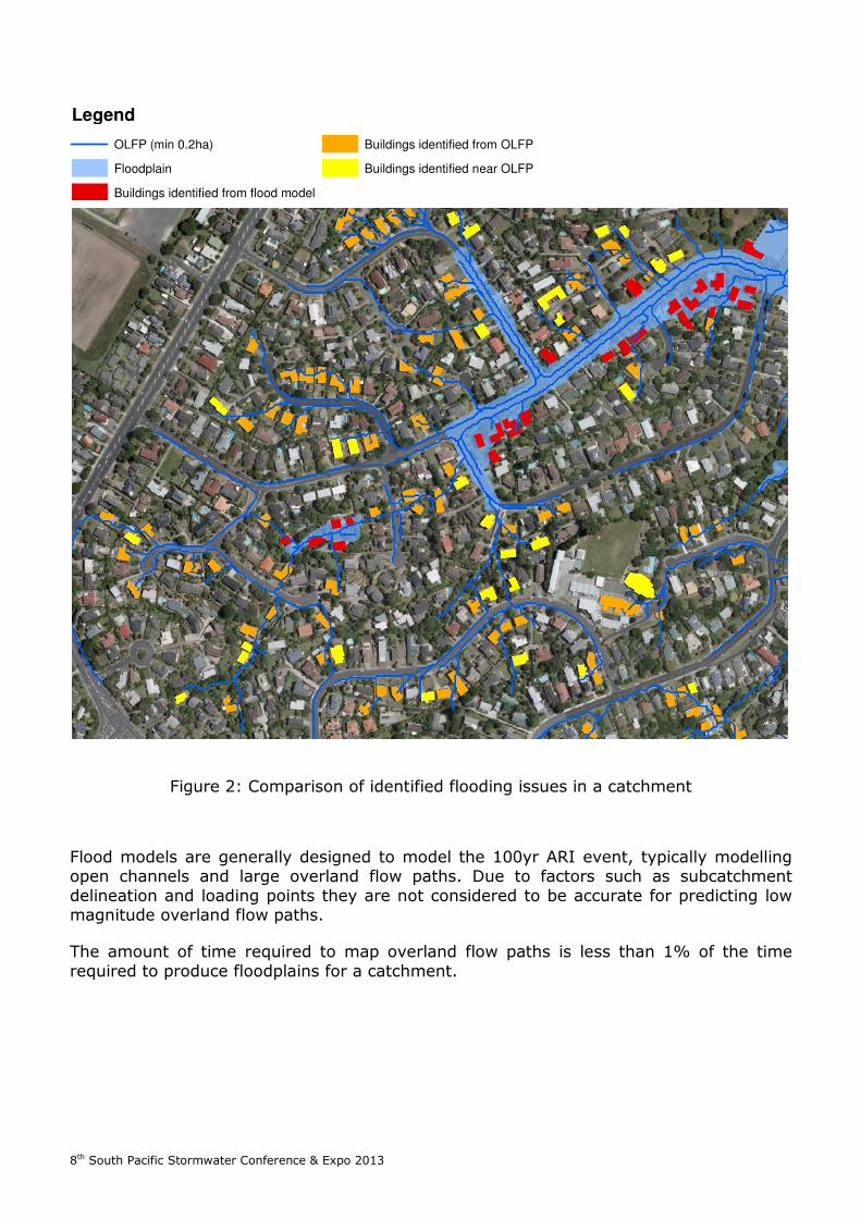
As an example in the area shown below 25 residential buildings were identified in the flood modelling study (i.e. in the extent of the floodplain), an extra 82 buildings have

predicted overland flow paths through them and an extra 29 buildings are within 2m of an overland flow path (refer to Figure 2). However, not all of these properties will have

issues in a 100yr ARI storm event (including those in the floodplains).


Figure 2: Comparison of identified flooding issues in a catchment

Flood models are generally designed to model the 100yr ARI event, typically modelling open channels and large overland flow paths. Due to factors such as subcatchment

delineation and loading points they are not considered to be accurate for predicting low magnitude overland flow paths.

The amount of time required to map overland flow paths is less than 1% of the time

required to produce floodplains for a catchment.

Legend

OLFP (min 0.2ha)

Floodplain

Buildings identified from flood model

Buildings identified from OLFP

Buildings identified near OLFP


2.4 METHODOLOGY Overland flow paths were mapped using the GIS package ARCGIS 10. The mapping

process utilised ModelBuilder to build various GIS models.

The simplified mapping process for overland flow paths is as follows:

• Start with a DEM representing the land (above ground features removed) • 'Fill' all depression areas in the topography (Fill tool) • Compute the flow direction of each cell (Flow Direction tool)

• Compute the upstream catchment area of each cell (Flow Accumulation tool) • Map the overland flow paths, using the flow direction, if the upstream catchment

area is greater than 2,000m² (Stream to Feature tool).

The process starts at the cell with the highest elevation and finds the lowest adjacent cell

and continues to do this downstream (refer to Figure 3). The flow direction shows the adjacent lowest cell. The flow accumulation (proportional to the catchment area) is the

number of cells that flow into the particular grid cell (refer to the red outlines in Figure 3). The process stops in the lowest point of a depression area (as all adjacent cells are higher than the current cell). Filling the grid removes all depression areas which allows a

continuous flow path to be mapped from the top of the catchment to the outlet at the bottom.

2.4.1 TERRAIN ADJUSTMENT

One identified issue with creating overland flow paths are that straight lines are created in the depression areas (refer to Figure 4). This comes about from using the filled grid to

produce overland flow paths. The filled DEM in depression areas have the same elevation value giving a flat surface. In large depressions (especially in urban areas) there is a need to know where the water will flow inside the depression extent.

Figure 3: Overland flow path mapping steps from topography to upstream

catchment area


Figure 4: 'Straight' overland flow paths in depression areas

To get accurate overland flow paths in depression areas the DEM needs to be adjusted to account for large culverts and natural ponding areas (refer to Figure 5 & Figure 6).

Figure 5: Digitised culverts to adjust the DEM and corrected overland flow paths

Legend

Overland flow paths Depression

Legend

Digitised culverts to adjust the DEM


Figure 6: Adjusted DEM to account for culverts

Three months was spent manually digitising over 2,500 line features to alter the terrain

across the region. An automated GIS process could not be used due to factors such as the incompleteness of the GIS data available.

Small depression areas, either constructed or natural ponding areas, were commonly found not to be 'drained' by a culvert and therefore a culvert couldn't be digitised to get accurate overland flow paths in these areas. These areas were generally at the sag points

of roads or in private property. In these cases the spill path, from the overland flow path dataset with straight lines in the depression, was digitised. Over half of the 2,500 lines

across the region were actually digitised overland flow paths.

The process to adjust the terrain is as follows:

• Identify the lowest point of the depression (using a difference grid) • Digitise from the lowest point, along the alignment of the culvert/stream, until the

DEM is lower than the lowest point of the depression

• Buffer the lines by at least the distance ��

• Burn the digitised line into the DEM by 20m (lower the elevation of the grid cells) • Fill the grid to create the new elevation surface to use for overland flow path

mapping.

Base DEM

DEM modified

for culvert


2.5 MODEL PROCESS

The GIS tools and models required to produce the overland flow paths were built in ModelBuilder, ARCGIS 10. A high specification HP Z800 workstation containing a 2.66GHz processor, 6 cores and 12GB of RAM was used for the processing. Each overland flow

path layer took up to 3 days to run and a number of weeks developing the methodology and models.

The sheer size of the Auckland region coupled with the detail of the mapping was a huge challenge to overcome and pushed computational capabilities to the limit. A 2m digital elevation model (DEM) grid was used for the region which contained 62,000 columns and

69,000 rows and was 16GB in size covering an approximate 4,900km2 area.

The region/datasets needed to be split into four different areas for computational

purposes and then later be remerged before creation of the lines.

Figure 7 below shows the GIS model to produce the flow directions and accumulation rasters without adjustment of the terrain and is one of six models used in the overland

flow path mapping process.

Figure 7: Overland flow path model (partial)

2.6 OUTPUT Two overland flow path layers were produced, one produced without terrain adjustment

(causing straight lines in the depression areas - refer to Figure 7) and the other produced using the adjustments to the terrain.


The unadjusted terrain model captures the spill path from each depression. Overlaying the two overland flow path layers ensures a full picture of the possible paths of stormwater in a storm event, i.e. overland flow, flow through the culvert and flow from

the crest of the depression (the spill path if the depression was to fill).

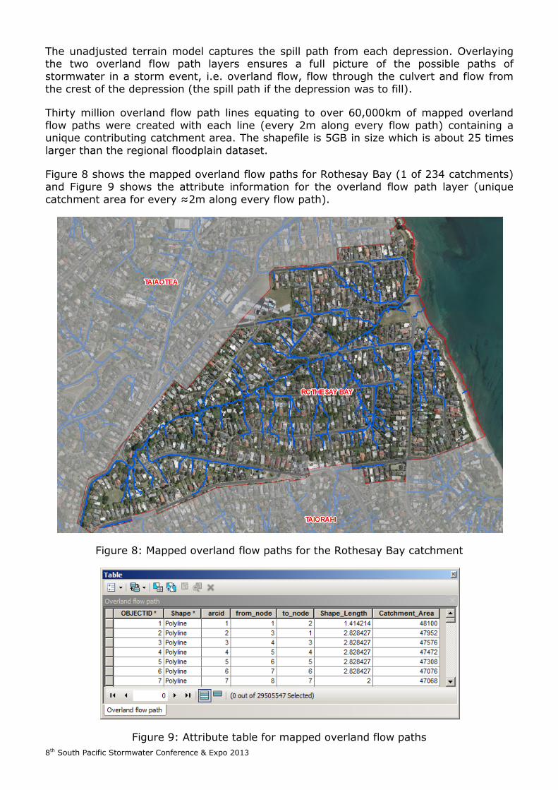
Thirty million overland flow path lines equating to over 60,000km of mapped overland

flow paths were created with each line (every 2m along every flow path) containing a unique contributing catchment area. The shapefile is 5GB in size which is about 25 times

larger than the regional floodplain dataset.

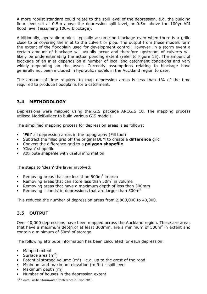
Figure 8 shows the mapped overland flow paths for Rothesay Bay (1 of 234 catchments) and Figure 9 shows the attribute information for the overland flow path layer (unique

catchment area for every ≈2m along every flow path).

Figure 8: Mapped overland flow paths for the Rothesay Bay catchment

Figure 9: Attribute table for mapped overland flow paths


2.7 USES

The common uses of mapped overland flow paths to date are:

• 'Flagging' developments that are occurring in overland flow paths to ensure adequate building provisions are considered.

• Identifying the existing properties potentially at risk of flooding due to overland flow. • Quick catchment/subcatchment boundary checks.

• Easy contributing catchment area check tool (unique catchment area available every 2m length along the flow path).

• Useful for flow calculations.

• Can be used to identify stream/rivers, e.g. overland flow paths with a contributing catchment area greater than 2ha can normally be considered a stream unless piped

(Kettle et al, 2013).

2.8 ASSUMPTIONS AND LIMITATIONS

The assumptions for the mapping process are that the:

• Lateral extent of the flow path is not considered (only the centreline is mapped). • Velocity of flow is not considered. • Depth of flow is not considered.

• Solid fences and walls are not considered. • Buildings are not considered.

Identified limitations to the process are the:

• Accuracy of the LiDAR data (e.g. the point density, equipment, process and the post-processing techniques). The accuracy of the mapped overland flow paths is highly

dependent on the quality of the LiDAR data. • Rural/Urban LiDAR (different LiDAR point densities for the rural and urban areas). • Grid or raster size used. Computationally a 2m grid was chosen as the appropriate

grid size for the region. A minor improvement would be realised if a smaller grid size was used, although far larger run times would result.

2.9 FUTURE WORK

Future work includes:

• Quantifying the 2yr, 10yr and 100yr ARI peak overland flow for existing and future land use and for existing and climate change adjusted rainfall (based on TP108).

Possible future work includes:

• Investigating the adjustment of the topography based on large commercial/industrial buildings as they are likely to divert the overland flow path around the building (say for buildings larger than 1,000m²).

• Investigating the adjustment of the topography based on a mapped stream shapefile to ensure there is accurate alignment along the stream especially in dense bush areas

and farm drains (no regional accurate stream shapefile currently exists).


3 TOPOGRAPHICAL DEPRESSION MAPPING

3.1 BACKGROUND

Depressions are areas that have a potential to pond or 'fill' up if the piped system was blocked or under capacity (wherever there are closed contours). They are the potential areal extent of the water up to crest level where water would spill downstream (instead

of continuing to pond up). Generally depressions are created due to the construction of a road perpendicular to a stream (refer to Figure 10). Large depressions are drained

typically by a culvert/inlet although some natural depressions (e.g. lakes) do occur.

Figure 10: Example depression extent with closed contours

3.2 BUSINESS DRIVERS Depressions were generated for the region primarily to:

• Identify flood prone areas - to influence development in these areas and to identify existing properties at risk of flooding

• Identify critical assets • Identify large dams (as defined in the Building Act 2004)


3.2.1 FLOOD PRONE AREAS Depression areas can be considered as flood prone areas. There is usually a floodplain/flood hazard area mapped at large depressions but their extent is usually

smaller than the depression extent. It is likely that the culvert will experience some form of blockage in a storm event and therefore reduce its capacity and capability to convey flows downstream causing a backing up of water upstream of the culvert and hence

raising flooding levels and increasing the flood extent. Applying a typical 0.5m freeboard for building floor levels on top of the computed 100yr ARI flood level is not sufficient to

account for factors like blockages in depression/ponding areas. These depression areas and associated spill levels have been identified around the region to influence intensification in these areas.

An example of a flood prone area is the depression upstream of Cartwright Road, Glen

Eden. In the 17th February 2012 storm event the Cartwright Road culvert collapsed causing the depression area upstream of Great North Road to fill up and spill over the top of the road (refer to Figure 11 and Figure 12). 18 habitable floors were flooded as a result.

Figure 11: Cartwright Road flooding


Figure 12: Overtopping of Great North Road (Cartwright Road flooding)

3.2.2 CRITICAL ASSETS

Auckland Council is currently in the process of identifying critical assets, predominately to ensure these assets are proactively maintained and perform to their potential at the start of a large storm event. These assets are often critical to the performance of the wider

stormwater system in a storm event. Mapped depressions are one input into an ongoing process to identify these assets.

3.2.3 LARGE DAMS

The definition of a dam, in part 1, subpart 7 of the Building Act 2004, is ambiguous and

it's uncertain as to whether road culverts fit into this description of a dam.

The Building Act 2004 and the Building (Dam Safety) Regulations 2008 form the framework for the Dam Safety Scheme. Under the Dam Safety Scheme, the owner of a

large dam is required to classify their dam and if considered medium or high in the Potential Impact Category (PIC) a Dam Safety Assurance Programme and an annual Dam Compliance Certificate needs to be submitted to the regional authority.


A large dam is defined as a "dam that retains 3 or more metres in depth and holds 20,000m3 or more volume of water".

The number of depressions greater than 3m in height and greater than 20,000m3 in volume in the Auckland region were identified by classifying the depression dataset. The

Dam Safety Scheme estimated 1,150 dams would be affected nationwide. 1,022 dam/depression areas would be considered as large dams in the Auckland region alone.

An amendment to the Bill proposes to split these dams into 'classifiable' and 'referable' dams due to the large number of dams (1,150) that they foresee the Dam Safety

Scheme would impact upon.

Classifiable dams would be those that: • are greater than 8m in height and greater than 20,000m3 or • can hold greater than 100,000m3 of water and greater than 3m in height.

Referable dams are those that are greater than 3m in height and hold more than

20,000m3 in volume (refer to Figure 13). Classifiable dams would automatically require a Dam Safety Assurance Programme and

an annual Dam Compliance Certificate to be submitted to the regional authority and referable dams would have to be assessed to determine whether they fall into the same

medium or high PIC (refer to Building Act, 2004). The Dam Safety Scheme has been deferred until July 2014.

Figure 13: Classifiable and referable dams


3.3 THE DIFFERENCE TO FLOODPLAIN MAPPING

Buildings constructed in depression areas, upstream of culverts, have an inherent residual risk of flooding. Often building levels are set based on the culvert acting at full capacity in a 100yr ARI event with the addition of freeboard (typically 0.5m in height).

There is generally no consideration given to the potential of blockage or collapse of the culvert before or during a storm event. Figure 15 is an example of a near full blockage of

a 1800mm diameter culvert which caused the depression in the 3rd of July 2012 storm event to fill to just below the spill crest (refer to Figure 15 for flood extent).

Figure 14: Level of blockage before and after rain event

Figure 15: Inundation of Sunnynook Park on the 3rd of July 2012


A more robust standard could relate to the spill level of the depression, e.g. the building floor level set at 0.5m above the depression spill level, or 0.5m above the 100yr ARI flood level (assuming 100% blockage).

Additionally, hydraulic models typically assume no blockage even when there is a grille

close to or covering the inlet to the culvert or pipe. The output from these models form the extent of the floodplain used for development control. However, in a storm event a

certain amount of blockage will usually occur and therefore upstream of culverts will likely be underestimating the actual ponding extent (refer to Figure 15). The amount of blockage of an inlet depends on a number of local and catchment conditions and vary

widely depending on the asset. Currently assumptions relating to blockage have generally not been included in hydraulic models in the Auckland region to date.

The amount of time required to map depression areas is less than 1% of the time required to produce floodplains for a catchment.

3.4 METHODOLOGY Depressions were mapped using the GIS package ARCGIS 10. The mapping process

utilised ModelBuilder to build various GIS models.

The simplified mapping process for depression areas is as follows: • 'Fill' all depression areas in the topography (Fill tool)

• Subtract the filled grid off the original DEM to create a difference grid • Convert the difference grid to a polygon shapefile

• 'Clean' shapefile • Attribute shapefile with useful information

The steps to 'clean' the layer involved:

• Removing areas that are less than 500m2 in area

• Removing areas that can store less than 50m3 in volume • Removing areas that have a maximum depth of less than 300mm • Removing 'islands' in depressions that are larger than 500m2

This reduced the number of depression areas from 2,800,000 to 40,000.

3.5 OUTPUT Over 40,000 depressions have been mapped across the Auckland region. These are areas

that have a maximum depth of at least 300mm, are a minimum of 500m2 in extent and contain a minimum of 50m3 of storage.

The following attribute information has been calculated for each depression:

• Mapped extent • Surface area (m2) • Potential storage volume (m3) - e.g. up to the crest of the road

• Minimum and maximum elevation (m RL) - spill level • Maximum depth (m)

• Number of houses in the depression extent


• Catchment area (m2) - based on the overland flow path layer • Amount of rainfall required to fill the depression (mm)

3.5.1 RAINFALL DEPTH CALCULATION

The amount of rainfall required to fill the depression was back calculated using the TP108 method and outlined below (ARC, 1999).

By rearranging the runoff depth formula (formula 1), the rainfall depth can be calculated using the quadratic formula (formula 2).

� = (� − ��)�(� − ��) + �

(1)

where: Q = runoff depth (mm)

P = rainfall depth (mm) S = potential maximum retention after runoff begins (mm)

Ia = initial abstraction (mm)

� = −� ± √�� − 4�2 + Ia

(2)

where:

b = - Q c = - QS

P = rainfall depth (mm) Ia = initial abstraction (mm)

The runoff depth (Q in mm) was calculated using the formula below.

� = 1000 × !"#$%

(3)

where: Vpot = Potential storage volume (m3)

A = Catchment area (m2)

Using an assumed catchment imperviousness of 70% (typical maximum probable development scenario for the urban area of Auckland) the curve number, CN, and soil

storage, S, can be calculated (refer to formula's 4 & 5). Curve numbers of 74 and 98 were used for pervious and impervious areas respectively.

The weighted curve number, CN, was calculated using the following formula.

&' =∑&'�%�%$#$ (4)


The soil storage, S, was calculated using the following formula.

� = )1000&' − 10*25.4 (5)

Calculations show 5% of the identified depressions can't possibly fill completely in a

100yr ARI event.

3.6 USES

The most common uses of mapped depressions to date are:

• Identifying flood prone areas. • Identifying critical assets. • Identifying large dams under the Building Act 2004.

• Identifying areas where there might be issues with LiDAR data (i.e. depressions shown in streams where there are no structures - LiDAR not able to penetrate dense

bush areas).

3.7 ASSUMPTIONS AND LIMITATIONS

The assumptions for the mapping process are that the:

• The runoff volume for a smaller or larger duration storm event is the same as the

TP108 24hr storm event (calculation of the rainfall depth required to fill the depression).

The limitations for the mapping process are that the:

• Statistics calculated for each depression (e.g. minimum and spill elevation) are

extracted from LiDAR. Therefore, the accuracy of the information is highly

dependent on the quality of the LiDAR data (e.g. the point density, equipment, process and the post-processing techniques).

• Extent of the depressions aren't necessarily the maximum extent in a storm event (i.e. if there is any flow over the road crest then the depression will be higher and larger in extent then shown).

• Grid or raster size used. Computationally a 2m grid was chosen as the appropriate grid size for the region. A small improvement would be evident if a smaller grid

size was used, although far larger run times would occur.

3.8 FUTURE WORK

Future work includes:

• Calculating stage/storage values for all the depressions to be used for 1D hydraulic

modelling and calculating the potential 100yr level (assuming a certain percentage of blockage of the outlet).

• Mapping the 100yr ARI extent for depressions that are very large (i.e. depressions that would require >100yr ARI rainfall depth in the catchment).

• Including the depressions layer in an appropriate way, using flood prone rules, in

the Unitary Plan. • Reproduce layer after LiDAR is re-flown.


4 COMBINED DATASETS

The overland flow path and depression layers provide very useful information in the catchment planning process to identify buildings at risk of flooding.

Figure 16 below shows the final output of the mapped overland flow paths and depressions. Overland flow paths are represented inside and outside of the depression

area. The mapped blue line leaving the depression area (via the digitised culvert) is the path of stormwater in low flows (i.e. through the pipe) and the mapped yellow line is the

potential spill path if the depression was to 'fill' up (due to blockage, inadequate pipe/inlet capacity or high peak flows) and spill downstream.

Figure 16 shows the spill path potentially affecting one property. Generally the spill path takes a similar route to the culvert/stream. It's important to identify the spill path

especially in areas where there is a divergence and properties are potentially at risk of flooding.

Figure 16: Mapped depression and overland flow paths


5 CONCLUSIONS

From the mapping work and recent experience in the use of these datasets the following conclusions can be made:

• Organisationally the overland flow path and depression layers provide a valuable

resource to Council staff and developers in planning and consenting for new and

existing developments. • Flood models only capture a portion of properties in a catchment at risk of flooding.

• Mapped overland flow paths and depression areas can identify potential flooding issues in catchments outside of the mapped floodplain or flood hazard areas.

• GIS can be a powerful and efficient tool in mapping overland flow paths and depression areas.

• The amount of time required to map overland flow paths and depression areas is less

than 2% of the time required to produce floodplains for the same catchment. • High resolution LiDAR data is vital to ensure reliable GIS data is produced.

• Flooding rules need to better allow for depression areas that have the capability to flood given partial or full blockage of culverts or pipe inlets.

6 ACKNOWLEDGEMENTS The authors would like to acknowledge Dr Ming Peng who was an integral part in developing the overland flow path methodology in GIS.

7 REFERENCES ARC (1999). Guidelines for stormwater runoff modelling in the Auckland Region (TP108).

Prepared for Auckland Regional Council by Beca Carter Hollings & Ferner Ltd.

Department of Building and Housing (2004). Building Act 2004. http://www.legislation.govt.nz/act/public/2004/0072/latest/DLM306036.html

Kettle, D; Irvine, J; Mayhew, I; Young, D (2013). The methodology for developing stormwater management areas for flow control for the Unitary Plan.

overland flow path and depression mapping for the auckland

Documents