Outsourcing, Structure of Firms, and WageInequality in the Market for Professional

Services

Jasmin Kantarevic∗

University of Toronto

August 8, 2004

Abstract

We view outsourcing as a relationship between firms that requirescommunication and coordination (management). Some workers havecomparative advantage in management, while others have compara-tive advantage in the production of outsourcing services. Productionskills of workers are observable, but there is symmetric learning aboutmanagement skills that varies by employment sector. Labour supplydecisions of workers, in addition to the outsourcing decisions of firms,determine the equilibrium extent of outsourcing, the size and hier-archical structure of firms, and the wage inequality. We show thatthese equilibrium outcomes tend to be positively correlated with eachother, and that they vary systematically with the market size. Weexamine these propositions empirically using the data on the marketfor legal services in the U.S. and find strong support for the model.The model can be used to interpret recent increases in both the extentof outsourcing and the wage inequality and attendant changes in thestructure of firms.

∗jkantare@chass.utoronto.ca. I thank Arthur Hosios and Aloysius Siow for their con-stant encouragement and many valuable comments. I also thank participants of seminarsat University of Toronto, Victoria University and York University. All remaining errorsare mine.

1

1 Introduction

Almost every firm has to decide what to produce in-house and what to pur-chase from the market (outsource). The outcome of this decision determinesthe boundaries of the firm, an issue that has been of keen interest to econo-mists since at least Coase (1932). Not surprisingly, there have been numeroustheoretical and empirical studies examining the determinants of outsourcingdecisions of firms and the variation in the extent of outsourcing across indus-tries and markets1.In recent years, there has been renewed interest in the subject because

of the spectacular growth in the extent of outsourcing over the last twodecades. However, the emphasis in many studies has shifted from analyzingthe determinants of outsourcing to understanding the impact of outsourcingon other important phenomena such as employment, wage structure, andincome inequality. For example, some researchers view the rise in the extentof outsourcing as an important determinant of the recent increase in the wageinequality2. While such efforts are pivotal to improving our understandingof the link between the extent of outsourcing and the wage inequality, theobserved correlation is open to alternative interpretations. Specifically, it isnot clear whether this correlation is causal or whether changes in both theextent of outsourcing and the wage inequality can be attributed to changesin some other factors such as the market size.What is needed to address this concern is a conceptual framework in which

the extent of outsourcing is jointly determined with other phenomena ofinterest. This paper makes first few steps in this direction. In particular, weanalyze the equilibrium process by which the extent of outsourcing, the wageinequality, and the structure of firms are jointly determined. In addition, wealso study the equilibrium relation of these variables with each other, andtheir dependency on the market size.The main conceptual innovation of the present paper is that we augment

an equilibriummodel of outsourcing with a model of labour supply of workersin the following way . We argue that the relationship between buyer firms,who are potential demanders of outsourcing services, and seller firms, who arepotential suppliers of these services, involves more than simply exchangingservices in the market. The buyer and seller firms have also to communicate

1Excellent surveys of this literature are provided by Perry (1988) and McMillan (1995)2See for example Dube and Kaplan (2001).

2

with each other and to coordinate their efforts in order to successfully com-plete outsourcing projects (a function called management hereafter). Thisassumption creates two types of jobs in the economy: production and man-agement. Some workers have comparative advantage in management, whileothers have comparative advantage in production. We assume that the infor-mation about management skills of workers is imperfect at the time workersfirst enter the labor market, but the market participants learn about theseskills as the workers accumulate experience. In addition, management skillsare valued relatively more in the seller firms because they service severalbuyer firms, while each buyer firm cares about completing its own outsourc-ing project only. For the same reason, the rate of learning about managementskills is relatively faster in the seller firms.Given this environment, the optimal behavior of buyers, sellers and work-

ers and their interaction at the market level determine the prices and quan-tities in the model: the prices of outsourcing services, the wage structure,the extent of outsourcing, and the structure of seller firms: their number,employment size and the ratio of production workers to managers (leverageratio).We show that in the equilibrium the extent of outsourcing and the wage

inequality are positively correlated. In addition, both of these variables tendto be positively associated with the employment size of seller firms, andinversely associated with the leverage ratio.The model also delivers predictions about the relationship of these vari-

ables with the market size. This relationship depends on whether the numberof workers in the market increases at a increasing or a decreasing rate withthe market size. In the first case, the extent of outsourcing, the wage in-equality, and the employment size of seller firms all vary directly with themarket size, while the leverage ratio varies inversely with the market size. Inthe second case, the predictions of the model are exactly the opposite.

In the empirical part of the paper, we use data on the market forlawyers from the 1992 Economic Census and the 1990 Census of Popula-tion and Housing to evaluate these predictions. We find strong support forthe model with respect to both pair-wise correlations between endogenousvariables and their relation with the market size.The remainder of the paper is organized as follows. Section 2 reviews

related literature in detail and delineates the contributions of the presentstudy. In section 3, we analyze a model in which workers have no role inthe outsourcing process. In this section, we assume that buyer and seller

3

firms can hire workers at the prevailing and exogenously determined wages.In Section 4, we enrich this model by introducing a model of labour supplyof workers, analyze the optimal behavior of buyers, sellers and workers, anddefine an outsourcing equilibrium. In section 5, we discuss the existence anduniqueness of the outsourcing equilibrium. We also identify the conditions forthe existence of two types of ’corner’ equilibria that may arise in the model;namely, the no outsourcing equilibrium, in which the buyer firms performall outsourcing services in-house, and the complete outsourcing equilibrium,in which the buyer firms outsource all tasks to the seller firms. Section 6discusses the comparative static results of the model. Section 7 describesthe data and outlines the methods for testing our empirical predictions, andsection 8 presents the results of the empirical tests. We conclude in section9.In the conclusion of this introductory section, we wish to emphasize that

our model of outsourcing is expected to fit markets for professional services,such as accounting and law, better than markets for other services. Thereason is that there is a clear distinction between production workers andmanagers in this market and there is empirical evidence of learning aboutinitially unobserved managerial skill in the seller firms. For example, lawyersin private law firms are usually divided into associates (junior lawyers) andpartners (senior lawyer), where the first group predominantly specializes inproduction of legal services and the latter group predominantly specializesin dealing with clients. Promotion of associates to partners is uncertain andusually takes several years as law firms learn about the potential of associatesin the partner positions.

2 Review of Related Literature

The objective of this section is to review literature on the extent of out-sourcing, the wage inequality and the structure of firms and to delineate thecontributions of the present study to this literature.In this review, we focus mainly on studies that analyze outsourcing and

on studies that link outsourcing to wage inequality and structure of firms.Our review is brief and we emphasize the most relevant studies only; theinterested reader may find more references in the sources cited in this sectionand in the bibliography section at the end of this paper.

Outsourcing

4

There is large theoretical and empirical literature on vertical integrationof firms and outsourcing. Excellent surveys are provided by Perry (1988)and McMillan (1995). Grossman and Helpman (2002) synthesize much ofthe previous literature in an equilibrium framework.For the purposes of our paper, three features of this literature are partic-

ularly relevant. First, many studies have emphasized some form of marketfailure as a potential determinant of outsourcing. Examples include monop-olistic markets for final goods, imperfect and asymmetric information, andtransaction costs due to incomplete contracting. Second, most studies haveanalyzed outsourcing as a bilateral relationship between a single buyer firmand a single seller firm. It was only recently that Grossman and Helpman(2002) studied outsourcing in an equilibrium framework with many firms ofeach type. Third, and to the best of our knowledge, none of the studiesexamined the supply decision of workers within a model of outsourcing.

In comparison to this literature, we analyze outsourcing within aneoclassical framework with competitive markets, perfect information andno transaction costs. Our claim is not that these factors are not important;rather, we simplify this side of the problem to gain better understandingof the importance of other factors in the outsourcing process. In particu-lar, we explicitly introduce a model of labour supply of workers to analyzethe process by which changes the labour market conditions influence the ex-tent of outsourcing. Therefore, our model simplifies the relationship betweenbuyer and seller firms, but gives an explicit role to workers in the outsourc-ing process. Consistent with recent contribution of Grossman and Helpman(2002), we also study outsourcing in an equilibrium framework.

Our model delivers reduced form predictions about the relation be-tween the extent of outsourcing and the market size that has received muchattention in the previous literature. This literature has advanced a num-ber of explanations for this relation. The most common explanation is thatthe extent of outsourcing increases in larger markets because firms may takeadvantage of economies of scale and learning and because there are moreopportunities for specialization in larger markets. Some studies also arguethat larger demand in big markets attracts entry of new seller firms, whichenhances competition and reduces costs of outsourcing. In Grossman andHelpman (2002), the market size is measured by the size of labor force andtheir model predicts that the extent of outsourcing increases in bigger mar-

5

kets because of larger demand for final goods3. In our model, the market sizealso affects the extent of outsourcing through larger demand for outsourcinggoods. In addition, the market size in our model also influences the extentof outsourcing indirectly through its impact on wages.

The empirical literature tends to find positive relationship betweenthe extent of outsourcing and the market size. For example, Abraham andTaylor (1996), using the data from Industrial Wage Survey conducted by theBureau of Labor Statistics between 1986 and 1987, find that the propensityof firms to outsource computer and accounting services is larger in metropol-itan areas in comparison to non-metropolitan areas, but these results do nothold for janitorial, machine maintenance, and engineering and drafting ser-vices. Ono (2001) uses data from the 1992 Annual Survey of Manufacturersand finds that the probability of outsourcing for white-collar services (adver-tising, bookkeeping and accounting, software and data processing, and legalservices) increases with an index of potential demand, but she finds no suchevidence for blue-collar services (building repair, machinery repair, refuseremoval).Our study contributes to this literature by providing new empirical evi-

dence on the relationship between the extent of outsourcing and the marketsize in the market for white-collar (legal) services. Our data set also allowsus to study outsourcing at more disaggregated level than was possible inthe previous studies. In particular, we examine the extent of outsourcingby banks and depository institutions, insurance companies, and real estatecompanies.

Wage InequalityIn the words of Katz and Autor, “studies of the wage structure are as old

as the economics profession”. In their excellent 1999 survey, they summa-rize evidence from many of these studies and also present a framework thatattributes changes in wage structure and earnings inequality to changes indemand and supply factors and institutions.

More closely related to our paper are studies that examine link be-tween outsourcing and wage inequality. These studies can be divided intothose that look into the effect of outsourcing on wage inequality and thosethat look into the effect of wage inequality on outsourcing. For example,

3This results holds only when the matching technology is increasing returns to scale.When the matching technology is constant returns to scale, the extent of outsourcing isindependent of the market size.

6

Abraham and Taylor (1996) find that the propensity to outsource janitorialservices is higher for firms that pay high wages . They interpret this resultas evidence that firms outsource in part to save on their labour costs. On theother hand, Dube and Kaplan (2001) use the CPS data between 1993 and2000 and document that janitors and security guards employed by Build-ing Service and Protective Service Contractors (sellers in our terminology)receive lower wages compared to janitors and guards who work for otheremployers.Our model also has implications for the relation between wage inequality

and the extent of outsourcing, but both of these variables are endogenouslydetermined in our model. In our empirical analysis, we present evidence onthe positive correlation between the extent of outsourcing and the wage in-equality, and also show that both of these variables are systematically relatedto the market size.

Our paper also provides a new explanation for the wage differentialbetween workers employed in buyer and seller firms. The previous literaturehas explained this wage differential in many ways. For example, the wagedifferential may arise due to differential unionization rates in the buyer andseller firms (Abraham and Taylor (1996)). The buyer firms may also payhigher wages to their internal workers, known in the literature as the ‘effi-ciency’ wages, to provide incentives to work harder, to reduce turnover, andto attract better applicants. The wage differential may also arise if the buyerand seller firms belong to different industries (the so called ’inter-industry’wage premium, analyzed in detail by Krueger and Summers (1987)) or be-cause of differences in the employment size between these two types of firms(the so called ‘employer size’ effect, analyzed by Brown and Medoff (1985)).In addition, the wage differential may arise because of differences betweenthe buyer and seller firms in the extent to which they are subject to vari-ous legislations regulating hiring and firing of workers. For example, Autor(2001) presents empirical evidence that the tightening of the employment-at-will regulations has raised costs of direct employment and thus led to a risein the use of temporary help services. As a result, workers employed in buyerand seller firms may receive different wages to compensate for differences inthe risk of losing jobs.In our model, the wage differential between workers employed in the buyer

and seller firms arises because jobs in these two types of firms differ in theextent to which they provide opportunities for accumulation of human capitaland future career advancement. In other words, our model builds on the

7

compensating wage differential literature (Rosen (198?)) and is determinedendogenously by the demand and supply factors. The institutional reasonsfor the wage differential, such as unionization, are likely to be less importantin the professional services sector such as legal services on which we focus inthis study.

Structure of Seller FirmsAs mentioned in the introduction, our model is expected to fit well in the

market for professional services such as accounting and law, and we reviewthe literature related to the structure of law firms here. For the purposesof this paper, this literature can be divided into three groups: (1) studiesthat examine aggregate employment and wages of lawyers at the marketlevel (e.g. Freeman (1975), Pashigian (1977), Rosen (1992)); (2) studiesthat analyze the mobility of lawyers between different employment sectors(e.g. Weisbrod (1983), Goddeeris (1988), Sauer (1998)); and (3) studiesthat analyze economics of law firms (e.g. Mc Chesney (1982), Spurr (1987),Gilson and Mnookin (1989), Carr and Mathewson (1990), Demougin andSiow (1994), and O’Flaherty and Siow (1995). The conceptual advantage ofthe first group of studies is that they consider both the demand and supplyside of the market, but their shortcoming is that they have less to say aboutthe mobility of lawyers and the structure of law firms. The other two groupsof studies overcome this shortcoming, but they typically consider only oneside of the market (the supply side in the second group, and the demandside in the third group). In this paper, we attempt to combine advantagesof all three groups of studies by analyzing both the employment decisions ofindividual lawyers and the decisions of law firms in an equilibrium framework.In addition, our model also incorporates choices of firms demanding legalservices, such as banks and insurance companies4 .

We borrow liberally from this literature and our debt will be clearthroughout the paper. In consequence, our model addresses a number ofissues that have been discussed in the literature. While many of our resultsare consistent with the results found in the literature, the main contribu-tion of this paper is that presents a unified framework for analyzing theseissues. Specifically, our model has implications for the number of law firms in

4With the exception of Pashigian (1982), most of the analyses of employment of lawyersin these firms (usually called in-house lawyers) have been conducted by members of legalprofession.

8

the market, their employment size, the promotion probability among juniorlawyers (associates), the mobility of lawyers among employment sectors, andthe wage differential between associates and senior lawyers (partners).

Our model of mobility of lawyers across employment sectors alsobuilds on recent contributions by Farber and Gibbons (1996) and Gibbons,Katz, Lemieux, and Parent (2002). Farber and Gibbons (1996) analyze amodel of symmetric learning about worker’s skills that are not observable byemployers when the worker enters the labor market. Gibbons etal. (2002)extend this model to allow returns to observable and unobservable skills tovary by the sector of employment. In this paper, we also consider a model inwhich workers’ skills can be divided into observable and unobservable skills,the returns to these skills vary by the employment sector, and there is asymmetric learning about the unobservable skills. In addition, we allow therate of learning about unobservable skills to vary among employment sectors.

3 A Model with Exogenous Wages

The main conceptual innovation of this paper is to explicitly model the roleof workers in the outsourcing process. To gain better insight into this role,we start in this section by analyzing a model of outsourcing in which workersplay no role at all. In the spirit of industrial organization literature, weview outsourcing as a relationship between two types of firms: buyer firms,who are potential demanders of outsourcing services, and seller firms, whoare potential suppliers of these services. In contrast to this literature, weanalyze the outsourcing problem using the neoclassical framework in whichmarkets are competitive, information is perfect, and there are no transactioncosts.The environment is quite simple. The economy is populated by only two

types of firms: buyers and sellers. The number of buyer firms is fixed at N,and the number of seller firms, denoted by S∗, is determined by a free entrycondition that will be described below. All buyer firms are identical, and allseller firms are identical, so we can discuss a representative buyer firm and arepresentative seller firm.The economy lasts for one period. At the beginning of the period, each

buyer firm receives a single outsourcing project. The project consists of aunit measure of identical tasks and must be completed in the same periodin which it is received. Tasks can be performed using labor as the only input

9

of production. In particular, a firm needs to employ n(x) workers to performx measure of tasks. n(.) is the only technology in the economy and it isavailable to both buyer and seller firms. We assume that n00(.) > 0, which isconsistent with diminishing marginal product of labour.Buyer firms can hire workers at the wage WB, and seller firms can hire

workers at the wage WS. Both WB and WS are exogenously determined.Lastly, tasks are exchanged in the competitive market for tasks at the priceP.This completes the description of the environment. We now discuss the

optimal behavior of firms and the market equilibrium conditions.The problem of a representative buyer firm is to decide what measure of

tasks to perform in-house (i.e. within the firm) and what measure of tasksto outsource (i.e. purchase from the seller firms) in order to minimize thecosts of completing the project. Formally, the problem can be stated as:

min0≤k≤1

CB(k) =WBn(k) + P (1− k)

The first-order necessary and sufficient condition for the interior5 opti-mum is:

WBn0(k∗) = P (3.1)

At the optimal k∗ the marginal cost of performing tasks in-house,WBn0(k∗),

is equated with the marginal cost of purchasing tasks from the market, P.The problem of a representative seller firm is to maximize its profits by

choosing what measure of tasks to perform:.

maxq≥0

Pq −WSn(q)

The first-order necessary and sufficient condition for the interior optimumis:

P =WSn0(q∗) (3.2)

5In this section, we focus on the equilibrium in which the buyer firms perform sometasks in-house, 1 > k∗ > 0, and outsource the remaining 1 − k∗ tasks to the seller firms.We discuss the no outsourcing equilibrium, in which the buyer firms perform all tasksin-house (k∗ = 1), and the complete outsourcing equilibrium, in which the buyer firmsoutsource all tasks (k∗ = 0), in section 5.

10

At the optimal q∗ the marginal cost of producing tasks, WSn0(q∗), is

equated to the marginal revenue from selling tasks to the buyer firms, P.Conditions (3.1) and (3.2) can be combined into:

WBn0(k∗) =WSn

0(q∗)

The marginal cost of performing tasks in the buyer firms is equated tothe marginal cost of performing tasks in the seller firms. This conditioncoincides with the socially optimal level of outsourcing, given the neoclassicalframework with competitive markets, perfect information, and no transactioncosts, and given that both types of firms have access to identical productiontechnology.The market for tasks clears when the demand for tasks by the buyer firms,

N (1− k∗) , equals the supply of tasks by the seller firms, S∗q∗ :

N (1− k∗) = S∗q∗ (3.3)

Lastly, the number of seller firms is determined by the condition that eachfirm attains normal economic profits. With diminishing returns to labour,the marginal costs, WSn

0(q), are larger than the average costs, WSn(q)/q, forany positive value of q, and the profits are always positive. To circumventthis problem, I introduce a fixed cost of entry for each seller firm, denotedby F . The number of seller firms is then determined by:

Pq∗ −WSn(q∗) = F (3.4)

The competitive outsourcing equilibrium with free entry can now be de-fined as a vector (P ∗, k∗, q∗, S∗) which satisfies equations (3.1) to (3.4). Thespecial case with n(x) = x2/2 is discussed in Appendix.What determines the extent of outsourcing in this model? First, the

incentive to outsource is stronger when the wage of workers employed bybuyer firms (WB) is higher and when the wage of workers employed by sellerfirms (WS) is lower. In a special case in which WB = WS, each of thebuyer and seller firms performs half of the outsourcing project. Second, thediminishing returns to labour assumption implies that it always takes fewerworkers to complete the project if the project is performed by two separateteams of workers rather than by one large team6. All else equal, outsourcing

6The proof is as follows. n0(.) > 0 implies n(x)/x is increasing in x, which thenimplies that n(x)/x < n(1)/1 for x < 1 and

Pn(x) < n(1)/1

Px = n(1). In particular,

11

a part of the project is less costly than completing the project entirely byeach buyer firm. Lastly, higher cost of entry (F ) discourages outsourcing assome seller firms exit the market, reduce the supply of tasks and thereforeraise the costs of outsourcing through higher equilibrium price of tasks.The number of buyer firms (N), a measure of the market size, does not

affect the extent of outsourcing in this model. The only adjustment to theincrease in the market size is the entry of new seller firms. However, theneutrality of the market size is specific to the model in which wages of workersare exogenously determined. In the next section, I show how the market sizeindirectly influences the extent of outsourcing through its role in determiningwage differentials.

4 A Model with Endogenous Wages

The basic model of the outsourcing discussed in the previous section demon-strated how the extent of outsourcing may depend on the exogenous wages atwhich buyer and seller firms can hire workers. Our objective in this sectionis to analyze how are these wages determined. We remain within the neo-classical framework by assuming perfect information, no transaction costs,and competitive markets (now also including labor markets).The basic model of outsourcing is enriched by introducing a model of

career choice of individuals. This model builds on contributions by Farberand Gibbons (1996) and Gibbons, Katz, Lemieux, and Parent (2002). Ingeneral terms, we consider a model in which workers’ skills can be dividedinto observable and unobservable skills, the returns to these skills vary bythe employment sector, there is a symmetric learning about the unobserv-able skills, and the rate of learning about unobservable skills to vary amongemployment sectors.The more specific ideas can be summarized as follows. The outsourc-

ing relationship between buyer and seller firms involves not only exchangingtasks in the market, but also communication and coordination (managementfor short). Some workers have comparative advantage in management, whileothers have comparative advantage in performing tasks. The informationabout management skills of workers is imperfect at the time workers firstenter the labor market, but the market participants learn about these skills

n(k∗) + n(1− k∗) < n(1) for k∗ ∈ (0, 1).

12

as the workers accumulate experience. Seller firms in general service sev-eral buyer firms, while each buyer firm cares only about completing its ownproject. For this reason, management skills are valued relatively more in theseller firms and the rate of learning about management skills is relativelyfaster in the seller firms.The remainder of this section develops these ideas in detail by analyzing

the decision problems of workers and each of a representative buyer firm anda representative seller firm. The section concludes by describing the marketequilibrium conditions in this extended model and by a formal definition ofthe competitive outsourcing equilibrium with free entry.

4.1 Individuals

Since learning takes time, the economy in this section lasts forever. Everyperiod L individuals are born who live for two periods. Individuals are riskneutral and do not discount future. In each period, individuals inelasticallysupply one unit of labor to the employer of their choice (a buyer or a sellerfirm) in order to maximize the expected present value of their lifetime income.Each individual is endowed with a two-dimensional vector of skills (A,B).

Each component of the skill vector takes the value of 1 if the individual hasthe relevant skill and the value of 0 otherwise. A represents the skill toperform tasks and B stands for the managerial skill.There are three important differences between A and B. First, all indi-

viduals have the skill to perform tasks, while only some individuals have themanagerial skill.Second, all market participants have perfect information about A, but

they learn about B only gradually. The rate of learning about B dependson whether the individual works for a buyer or a seller firm. Specifically,individuals who work in the seller firms for one period receive a signal thatreveals their B perfectly, while individuals who work in the buyer firms learnnothing about B.The prior probability that an individual has the managerial skill is given

by Pr[B = 1] = µ. µ can be interpreted as the index of all individual’scharacteristics positively correlated with the promotion probability, such aseducation, genetic ability, ambition, and social skills7. For concreteness, I

7For example, Sauer (1998) shows that other correlates of the promotion probabilityin law firms include the performance in law school (GPA, class rank, participation in

13

will refer to µ as ability. The distribution of ability in each generation isgiven by a time-invariant distribution function G(.) with associated densityg(.).The third difference between A and B is that buyer and seller firms value

these skills differently. In particular, the managerial skill is not used in thebuyer firms. Individuals who work in these firms perform tasks only and earnthe in-house wage WB in each period.In contrast, workers in the seller firms perform tasks in the first period

and earn the training wageWS.During this period, the information about themanagerial skill is perfectly revealed. Individuals with B = 1 are promotedto managerial positions in the second period and earn the managerial wageWM . Individuals who are not promoted can either stay in the seller firmsand earn WS performing tasks, or they can move to a buyer firm. As I willshow shortly, unsuccessful trainees always have an incentive to leave the sellerfirms. The assumption that these trainees can always find jobs in the buyerfirms implies full employment in each period. For simplicity, I assume thatthere are no mobility costs to individuals, nor hiring or firing costs to firms.The career choices of individuals can now be described as follows. The

income stream of an individual in his first period of life (a young individual)in the buyer firms is 2WB. The expected income stream of a young individualin the seller firms isWS+µWM+[1−µ]WB. The marginal young worker withability level µ∗ is indifferent between working for a seller firm and workingfor a buyer firm, which implies that the training wage satisfies the followingcondition:

WS =WB − µ∗[WM −WB] (4.1)

From equation (4.1) it is easy to see that in any equilibrium in which sellerfirms employ some managers, it must be the case that WM > WB > WS. IfWB > max{WM ,WS}, all individuals would want to work for the buyer firmsonly. If WS > WM , no trainee would ever want to become a manager.The result that WB > WS, even though individuals have identical skill

to perform tasks, reflects the option value of training jobs in the seller firms.These jobs offer an opportunity to learn about one’s potential in a high-wage managerial position, and individuals are willing to ’invest’ early intheir careers by accepting lower wages. Stated alternatively, the buyer firmsoffer higher wages to compensate individuals for the lack of opportunities for

mout courts, graduate school prior to the law school) and family characteristics (whethera parent was attorney).

14

career advancement. This result closely resembles Rosen’s (1972) result thatworkers in jobs with higher potential to accumulate human capital are willingto accept greater reduction in their wages early in their careers to increasetheir earnings in the future. In my model, the form of human capital islearning about one’s managerial skill.The sorting of young individuals between buyer and seller firms is based

on their ability. All young individuals with µ ≥ µ∗ work for the seller firms,while all young individuals with µ < µ∗ work for the buyer firms.Individuals in their second period of life (old individuals) who worked for

the seller firms and who were promoted choose to stay in the seller firmsbecause WM > WB. All other old individuals work for the buyer firms. Inparticular, unsuccessful trainees voluntarily choose to leave the seller firmsbecause WB > WS.

4.2 Seller Firms

In this extended model, the seller firms live forever and employ two typesof workers: trainees and managers. Trainees specialize in performing tasks,while managers specialize in providing client services (i.e. communication,coordination, etc.). To capture this distinction between the role of traineesand managers in a simple way, decompose the total measure of tasks per-formed by seller firms as q = B • kS, where B is the number of clients(i.e. buyer firms) each seller firm services, and kS is the measure of tasksperformed for each client.The costs of servicing B clients and performing kS tasks for each client

can be represented as WSn(BkS) + WMm(B). WS is the training wage,WM is the managerial wage, n(.) is the number of trainees, and m(.) is thenumber of managers. n(.) has identical properties as in the previous section.m(.) summarizes the management technology. Similar to n(.), I assume thatm00(.) > 0, consistent with diminishing returns to labor in management.For the purpose of analytical simplification, I assume that seller firms set

a separate team of trainees for each client they service. With this assumption,each project in the economy is completed by two teams of workers: a team oftrainees in the seller firms and a team of in-house workers in the buyer firms.These two teams are identical except for the wage rate at which workersin each team can be hired. This assumption also allows a complementaryinterpretation of what managers in this model do. Since each seller firmservices B clients, and each client is serviced by one team of trainees, the

15

communication and coordination function of managers is closely related totheir function of managing and supervising teams of trainees.The analytical advantage of this assumption arises because the production

and management decisions of seller firms can be separated into two stages.In the first stage, the seller firms decide what measure of tasks to perform foreach client, and in the second stage, they decide how many clients to service.With the separability of the production and management decisions, the costfunction becomes WSBn(kS) +WMm(B).In this model, outsourcing is similar to a tied-in sale, because the buyer

firms cannot purchase tasks without also purchasing client services. Eachcomponent of the tied-in sale is priced competitively. Specifically, the marketfor tasks determines the unit price of tasks PK , as in the previous section, andthe market for client services establishes the client fee PB. For any arbitrarynumber of clients B and any measure of tasks for each client kS, the revenuesof seller firms are equal to B(PKkS + PB).A representative seller firm now maximizes its profits by deciding in each

period8 on how many clients to service and what measure of tasks to performfor each client. Formally, the problem is:

max0≤kS≤1, B≥0

Π(kS, B) = B[PKkS −WSn(kS) + PB]−WMm(B)

The first-order necessary and sufficient conditions for the interior9 solu-tion are:

WSn0(k∗S) = PK (4.2)

PKk∗S −WSn(k

∗S) + PB = WMm0(B∗) (4.3)

Equation (4.2) is similar to the first-order condition in the basic model: atthe optimal k∗S, the marginal cost of performing an additional task,WSn

0(k∗S),is equal to its marginal revenue, P. An important property of the solution

8That is, we assume that tasks cannot be stored and in each period the seller firms faceidentical problem. This assumption excludes the possibility of strategic behaviour overtime, but is adopted for analytical simplification.

9As in the previous section, we focus on the equilibrium in which buyer firms outsourcesome tasks and perform some task inhouse. The next section discusses other types ofequilibria in the model.

16

is that k∗S depends only on the training wage and the price of tasks and isindependent of the managerial wage and the client fee. This result is dueto the assumption that the production decision can be separated from themanagement decision. Equation (4.3) states that at the optimal B∗, themarginal profit (the left-hand side) and the marginal cost, WMm0(B∗), areset equal to each other.Lastly, the number of seller firms is determined as in the previous section

by the condition that each seller firms attains normal economic profits:

Π(k∗S, B∗) = F (4.4)

4.3 Buyer Firms

Buyer firms also live forever. In this extended model, a representative buyerfirm has to pay a fixed client fee to each seller firm from whom it purchasesany tasks. The client fee is like a fixed cost of outsourcing, and the buyerfirm will minimize its outsourcing costs by dealing with a single seller firm.Given the choice of how many seller firms to deal with, the problem of arepresentative buyer firms in each period10 is:

min0≤kB≤1

WBn(kB) + PK(1− kB) + PB

The first-order necessary and sufficient condition for the interior solutionis:

WBn0(k∗B) = PK (4.5)

Equation (4.5) is identical to the first-order condition for the buyer’sproblem in the model of the previous section: At the optimal k∗B the marginalcost of performing tasks in-house, WBn

0(k∗B), is equated with the marginalcost of purchasing tasks from the market, P .

4.4 Equilibrium

In this model, there are two outsourcing markets (for tasks and client ser-vices) and three labour markets (for trainees, managers, and in-house work-

10Buyer firms face identical problem in each period due to our assumption that theoutsourcing project must be completed in the same period in which it is received. Again,this assumption is for analytical simplification.

17

ers). The market clearing conditions are as follows.In the outsourcing markets, the buyer firms demand services of N seller

firms and each buyer firm demands 1 − k∗B tasks. Seller firms supply clientservices to S∗B∗ clients and perform k∗S tasks for each client. The equilibriumconditions in the market for tasks and the market for client services are,respectively, :

1− k∗B = k∗S (4.6)

N = B∗S∗ (4.7)

In the labour markets, the seller firms demand S∗B∗n(k∗S) trainees andS∗m(B∗) managers, while the buyer firms demand Nn(k∗B) in-house workers.To derive the supply of trainees and managers, let ∆(µ∗) ≡ 1−G(µ∗) be thefraction of individuals for whom µ ≥ µ∗, and let Λ(µ∗) ≡ E[µ|µ ≥ µ∗] theaverage probability of promotion among trainees. Using this notation, thesupply of trainees is ∆(µ∗)L and the supply of managers is Λ(µ∗)∆(µ∗)L. Allother individuals work in the buyer firms.The clearing conditions in the market for trainees, the market for in-house

workers, and the market for managers are, respectively:

S∗B∗n(k∗S) = ∆(µ∗)L (4.8)

Nn(k∗B) = 2L−∆(µ∗)L− Λ(µ∗)∆(µ∗)L (4.9)

S∗m(B∗) = Λ(µ∗)∆(µ∗)L (4.10)

We conclude this section with a definition of the outsourcing equilibrium.

Definition. The competitive outsourcing equilibrium with free entry isa vector of prices (P ∗K , P

∗B,W

∗B,W

∗S ,W

∗M) and quantities (k

∗S, k

∗B, B

∗, S∗, µ∗)which satisfies conditions (4.1) to (4.10).

5 Types of Equilibria

In this section, we discuss the existence and uniqueness of the competitiveoutsourcing equilibrium with free entry. We also identify the conditions for

18

the existence of two types of ’corner’ equilibria that may arise in the model,namely, the no outsourcing equilibrium, in which the buyer firms perform alltasks in-house (k∗B = 1), and the complete outsourcing equilibrium, in whichthe buyer firms outsource all tasks to the seller firms (k∗B = 0).The strategy for proving the existence of the competitive outsourcing

equilibrium with free entry consists of first showing how the system of equa-tions (4.1) to (4.10) can be reduced to a single equation, and then analyzingthe conditions under which this equation has a solution. The first step then isto combine the equilibrium conditions in the market for trainees, the marketfor in-house workers, and the market for client services, and then express theequilibrium in the market for tasks as follows11:

1− kB

µµ∗;

L

N

¶− kS

µµ∗;

L

N

¶= 0 (5.1)

In this equation, kB (.) is a set of all pairs (kB, µ) such that the marketfor in-house workers clears. kS (.) is a set of all pairs of (kS, µ) such that themarket for trainees and the market for client services clear. Equation (5.1)picks µ among these pairs that is also consistent with the equilibrium in themarket for tasks.Define the left-hand side of (5.1) for any arbitrary µ as M(µ), which can

be interpreted as the excess demand for tasks. The competitive outsourcingequilibriumwith free entry exists if there is a µ∗ ∈ (0, 1) such thatM(µ∗) = 0.

M is continuous in µ. In the appendix, we also show thatM is monotoni-cally decreasing in µ, given the equilibrium condition that the in-house wageexceeds the training wage (WB > WS). Therefore, the necessary and sufficientcondition for the existence of the competitive partial outsourcing equilibriumis:

M (0; l) > 0 > M (1; l) (5.2)

where l is defined as L/N, the number of workers in each generation perbuyer firm in the market. The interpretation of this condition is straight-forward. If all individuals were allocated to the seller firms (µ = 0), therewould be an excess demand for tasks (i.e. teams of trainees in the seller firmswould perform fewer tasks than is necessary to complete the project), andif all individuals were allocated to the buyer firms (µ = 1), there would bean excess supply of tasks. Note also that when (5.2) holds, the competitive

11Equation (4.1) is derived explicitly in the appendix.

19

outsourcing equilibrium is unique because M is monotonically decreasing inµ. The competitive outsourcing equilibrium is illustrated in graph 1.We now further explore the existence condition and discuss the ’cor-

ner’equilibria in the model. In the appendix, we show that M decreaseswith l. Therefore, the competitive outsourcing equilibrium with free entrycan exist only if l lies in the appropriate range: l ∈ (lmin, lmax), where lminand lmax are implicitly defined by:

M (0; lmin) = 0

M (1; lmax) = 0 (5.3)

Again, these conditions are intuitive. When there are very few workers inthe market, it is impossible to complete all outsourcing projects; and whenthere are very many workers in the market, it is impossible to attain full em-ployment. When l = lmin, we have the ’no outsourcing’ equilibrium. With fewworkers in the market, allocating any workers to the management functiondoes not increase production of tasks, and since outsourcing is not possiblewithout management, the only solution is to have outsourcing projects per-formed entirely in-house. When l = lmax, the only possible equilibrium is the’complete outsourcing’ equilibrium.We summarize this discussion in the following proposition.

Proposition 1 (Types of equilibria) When l = lmin, buyer firms perform alltasks in-house; when l ∈ (lmin, lmax), buyer firms perform some tasks in-houseand outsource the rest to seller firms; and when l = lmax, the buyer firmsoutsource all tasks. lmin and lmax are implicitly defined in equation (5.3).

The model does not address the situation in which l lies outside theinterval [lmin,lmax]. This case can be interpret as a disequilibrium situation:either there is some unemployment (when l > lmax) or some outsourcingprojects cannot be completed (when l < lmin).The equilibrium interpretation can be preserved if we extend the model

in either of the following directions. The first is to allow outsourcing acrossmarkets. In this case, the buyer firms in markets with l < lmin may purchasetasks from the seller firms located in markets with l > lmax. We leave thisextension to future research.The second case is to allow mobility of the individuals across markets,

so individuals may move from the markets in which l > lmax to markets in

20

which l < lmin. In this case, the mobility of individuals ensures that l lies inthe appropriate range. A simple way to capture this idea is to endogenizethe measure of workers in each generation as L = L(N). L0(N) is likely tobe positive as individuals move from the smaller to larger markets to keep lin the interval [lmin,lmax]. The sign of L00(N) is less clear. If there are somerestrictions on the mobility of workers, then L00(N) will be negative as theincrease in the market size will be offset by increasing the number of workersbut at a decreasing rate. On the other hand, if there are increasing returnsto workers from locating in larger markets (e.g. lower search costs), then wecan expect that L00(N) will be positive.

6 Comparative Statics

The endogenous variables in the can be divided into four groups: (1) theextent of outsourcing (k∗B, k

∗S, B

∗); (2) the cost of outsourcing (P ∗K , P∗B); (3)

the wage distribution (W ∗B,W

∗S ,W

∗M); and (4) the number and hiearchical

structure of seller firms (S∗, µ∗). The analytical comparative static resultsare available for all of these variables except for P ∗K and P

∗B and these results

are discussed in propositions (2) to (4). We also numerically solve the modelfor a special case with n(k) = k2/2, m(B) = B2/2 and G(µ) = µ and presenta full set of comparative static results for this case.The model includes three parameters of interest: the size of each gen-

eration of individuals, L; the number of buyer firms, N ; and the fixed costof entry, F . We present comparative results for these parameters and alsodiscuss the results for N when there is free mobility of workers (i.e. whenL = L(N)). All proofs are delegated to the appendix.

Proposition 2 When there is an increase in the size of each generation ofindividuals (or a decrease in the number of buyer firms), then: (i) the extentof outsourcing increases, (ii) each seller firm services more clients, (iii) thewage differential between in-house workers and trainees increases, (iv) themanagerial wage falls, (v) the number of seller firms in the market falls, and(vi) the promotion probability among trainees falls.

The increase in the size of workers in each generation or a decrease inthe number of buyer firms both shift the excess demand curve in graph 1downward, and the new equilibrium level of µ falls (that is, some in-houseworkers are reallocated to the seller firms). The intuition is as follows. In

21

the equilibrium, the marginal costs of performing tasks between teams ofin-house workers in the buyer firms and teams of trainees in the seller firmsare equalized, which can be expressed as:

WBn0(kB) =WSn

0(kS)

where we omit the stars denoting the equilibrium values. SinceWS < WB,the marginal product of trainees must be smaller than the marginal productof in-house workers, or n0(kS) > n0(kB). In addition, since the marginal prod-uct is decreasing (or n00(.) >), reallocating an in-house worker to a trainingjob in a seller firm (i.e. a fall in µ) will decrease the total production of in-house workers by more than it will increase the total production of trainees.In other words, the total production of tasks will fall following the realloca-tion of workers and the change in excess demand for tasks will be positive.Note that this result is driven by two factors: first, the wage differentialbetween in-house workers and trainees, which arises because training jobsprovide an opportunity to learn about one’s managerial ability; and second,the diminishing returns property of the production technology.Once we identify the direction of movement of workers between the buyer

and seller firms in response to changes in N or L, the results in proposition(2) are easy to understand. The workers who move from the buyer firmscome from the lower end of the ability distribution and the average abilityof trainees (and their probability of promotion to managers) falls. Teams oftrainees become larger relative to teams of inhouse workers, and the frac-tion of outsourcing project performed by seller firms increases. The wagedifferential between in-house workers and trainees also increases due to themovement of workers from the buyer to seller firms. Since seller firms employmore trainees, the supply of managers in the future periods also increases,their wages decrease and the seller firms employ more managers and servicemore clients. Lastly, since the number of clients has not changed and eachseller firm services more clients, this implies that there are fewer seller firmsin the market.The response of endogenous variables to changes in l = L/N in a special

case with n(k) = k2/2, m(B) = B2/2 and G(µ) = µ are presented in figure112. This figure confirms the results presented in proposition (2) and shows

12In this case, the equilibrium exists if the equation

1− l1/2³(2(1− µ∗)1/2 + (1 + µ∗

´) = 0

22

that an increase in the size of each generation of individuals (or a decreasein the number of buyer firms) also leads to lower price of tasks and higherclient fee.

Proposition 3 Suppose L = L(N). If L00(.) > 0, then the comparative sta-tics with respect to N are identical as those for L in proposition (2). WhenL00(.) < 0, the results are opposite of those for L in proposition (2). WhenL00(.) = 0, the only effect of N is the increase in the number of seller firmsin the market.

These results are also intuitive. In this case, the increase in the num-ber of buyer firms affect endogenous variables through two channels: first,by increasing the demand for tasks, and second, by increasing the numberof workers in the market. When the number of workers increases at an in-creasing rate with the number of buyer firms, there will be a positive changein excess demand for tasks, and conversely in the case when the number ofworkers increases at a decreasing rate. When the increase in the number ofworkers is constant, there will be no change in the excess demand and theonly adjustment to the increase in the number of buyer firms will be entry ofnew seller firms. Note that this last case is identical to the result obtainedin the model with exogenous wages.

Proposition 4 When the fixed cost of entry increases, then (i) the manage-rial wage increases, (ii) the training wage increases, (iii) the in-house wageincreases, and (iv) the price of tasks increases. The extent of outsourcing,the number of clients per seller firm, the number of seller firms, and the pro-motion probability among trainees are all independent of changes in the fixedcosts of entry.

In the special case with n(k) = k2/2, m(B) = B2/2 and G(µ) = µ, itcan be shown that all prices and wages considered in proposition (4) areincreasing linear functions of F. On the other hand, the relation between thefixed client fee and F can be either positive or negative, depending on theassumed values for L and N.

has a solution. The fixed cost of entry F is normalized to 1. The existence of equilibriumrequires that l ∈ [0.16, 0.25] and that µ∗ be consistent with WB > WS which implies thatµ∗ ∈ [0, 0.236].

23

7 Data and Methods

The objective of the following two sections is to empirically evaluate a sub-set of propositions derived from our theoretical model of outsourcing. Inthis section, we describe two methods to test our empirical propositions anddescribe the data used in the analysis. The next section then presents thedetailed results of the empirical tests.

7.1 Methods

The propositions to be tested are summarized in table 113. According tothe model, the endogenous variables of interest should be positively corre-lated, independent of the sign of L00(N). In addition, all endogenous variablesmust vary in the same direction with the market size, regardless of the ex-act relationship between the market size and the size of labor force. WhenL00(N) > 0, the endogenous variables will vary positively with the marketsize, and conversely in the case when L00(N) < 0. Therefore, the first methodfor evaluating our empirical propositions is to test whether pair-wise correla-tions between endogenous variables are positive and whether these variablesvary in the same direction with the market size.

The second method is more rigorous and consists of evaluating therelationship between each of the endogenous variables and the market size ina multivariate regression framework. This method recognizes that variationsin the endogenous variables across markets depend not only on the marketsize, but also on a host of other variables such as the composition of demandand the characteristics of labor force.

In particular, for each of the endogenous variables we estimate amodel of the following form:

Ym = α0 + α1Xm + α2Zm + εm (7.1)

where Y indicates the endogenous variable of interest, X is the marketsize, and Z includes a set of other expected determinants of Y . The variablesare defined at the market level, denoted by m. ε is the error term.

13The empirical definitions of the endogenous variables and the market size will bediscussed in futher detail below. The definitons of these variables in terms of the theoreticalconstructs of the model is discussed in the appendix.

24

According to the predictions of the model, the coefficient a1 should be ofthe same sign for all endogenous variables examined. In addition, α1 > 0 ifL00(N) > 0, and conversely , α1 < 0 if L00(N) < 0.

Model (7.1) can be estimated using the ordinary least squares method.However, the model with the extent of outsourcing is a bit more involved be-cause in some markets all production may be outsourced14. This case can betreated in two ways. First, we can estimate model (7.1) and interpret a1 asthe relationship between the extent of outsourcing and the market size, giventhat buyer firms produce some services in-house (i.e. ∂E[Y |Y > 0]/∂X ).This case corresponds to the competitive outsourcing equilibrium with freeentry discussed in the previous sections. Second, we can also estimate theunconditional relationship between the extent of outsourcing and the marketsize (i.e. ∂E[Y ]/∂X). In this case, we first estimate the probability thatthe buyer firms employ in-house workers, Pr(Ym > 0), using any methodfor discrete choice models such as probit or logit. In the second step, weestimate model (7.1) as before. Using the estimates from these two models,we can then calculate the expected extent of outsourcing in all markets asPr(Ym > 0)E[Y |Y > 0]. In our empirical analysis, we will examine boththe conditional and unconditional relation between the extent of outsourcingand the market size.

7.2 Data

Our empirical analysis focuses on the market for legal services for two im-portant reasons. First, we have developed our model based on the extensiveliterature that describes the structure of this market and most of theoreticalconstructs of our model can be easily translated into their empirical coun-terparts in this market. Second, the available data for this market allows usnot only to examine the structure of seller firms in great detail, but also toanalyze the extent of outsourcing at much more disaggregated level than waspossible in the previous empirical studies.

We use three data sets: the Legal Services portion of the 1992 Eco-nomic Census, the 1990 Census of Population and Housing, and the Bureauof Economic Analysis (BEA). The 1992 Economic Census provides a wealthof information on the structure of private law firms, while the 1990 Census

14The other possibility that all production takes place in-house is of little empiricalimportance.

25

provides detailed information about the characteristics of lawyers. In combi-nation, these two data sets allow us to construct all empirical measures forour endogenous variables. We use the BEA estimates to construct a varietyof measures for the market size.The Legal Services portion of the 1992 Economic Census covers all law

establishments with at least $1,000 in annual revenues, which practicallyimplies that every law office in the United States is included. In 1992, therewere 151,737 law offices and 147,130 law firms, employing 435,219 lawyersand 665,480 non-lawyers. The definition of law firms and law offices is almostidentical since only about 2% of law firms have more than one office.

The Census collects variety of establishment-level information aboutlaw offices. Law offices report their annual revenues by the source (indi-viduals, businesses, and government), the annual payroll by job categories(associates, paraprofessionals, non-legal managers and other employees) andthe number of individuals in each job category, including partners and soleproprietors. The unique feature of the data is that it also reports the numberof lawyers specializing in different fields of law practice, such as banking lawand insurance law. The data are published at the market level (where themarket is defined as MSA or PMSA) in the Sources of Receipts and Rev-enues and Miscellaneous Subjects parts of the Census of Services publicationprogram.The 1990 5 % Census of Population and Housing contains detailed infor-

mation about occupation and industry of individuals. For the purposes ofthis analysis, I have included information on all lawyers and judges who donot reside in group quarters, who are employed and who are not in school.This sample consists of 27,985 lawyers and judges. 15 % of these lawyerswere employed in the government sector, 75% worked in the legal services in-dustry and 10% worked in other private industries. Among lawyers employedin non-legal industries, about 35% worked in the banking and credit sector(8.85%), the insurance sector (17.78%), and the real estate sector (8.09%).The Census provides data at the individual level, but the estimates at theMSA/PMSA level can be obtained by using the Census sampling weightsand the place of residence.

Lastly, the BEA provides estimates of the population size, the privateemployment, the gross personal income, and the employment in each of themain nine industries at the MSA/PMSA level.

26

7.3 Description of Variables

7.3.1 Endogenous variables

Our initial empirical measure of the extent of outsourcing is the ratio of as-sociates and partners in private law firms to the in-house lawyers employedin the business sector. The main concern with this measure is that lawyersemployed in the private law firms tend to service not only business clients,but also individuals and various government agencies. To circumvent thisproblem, I refine my empirical measure of outsourcing by exploiting the in-formation about the field of specialization of lawyers in the 1992 EconomicCensus. I focus on three fields of specialization: the banking and commerciallaw, the insurance law, and the real estate law. Lawyers specialized in thesefields service primarily banks, depository institutions, insurance companiesand real estate companies15. However, the 1992 Economic Census does notidentify whether these specialized lawyers are associates or partners, and ourempirical measure of outsourcing includes both associates and partners whoare specialized in these fields. The information on the number of in-houselawyers who are employed in the banking, insurance and real estate sectorsis available from the 1990 Census of Population and Housing16. Our refinedmeasure of the extent of outsourcing is then the number of lawyers in privatelaw firms specialized in field j divided by the number of lawyers employedin business sector j, where j stands for all fields, banking, insurance, or realestate. Since this ratio is not well defined for markets in which there areno in-house lawyers, we employ the inverse of this measure in the empiricalanalysis.The employment size of a private law firms, our second endogenous vari-

able of interest, is calculated as the number of associate lawyers and partnersdivided by the number of private law firms, available from the 1992 EconomicCensus.The ratio of trainees to managers is measured as the ratio of associates

15Some lawyers specialized in real estate law are also expected to service individualclients.16The two-year difference between the Economic Census and the Census of Population

should not be of great concern because temporal variation in the extent of outsourcing istypically smaller than the across-markets variation, specially considered than in our datathere is only two-year difference. Nevertheless, we have examined this by inflating thenumber of in-house lawyers in the 1990 Census by the rate of growth of employment in thefinancial sector between 1990 and 1992 and found no significant changes in our results.

27

to partners in private law firms. This measure is also readily constructedfrom the 1992 Economic Census. However, the quirk of the data is that notall private law firms have both partners and associates. In particular, theprofessional service organizations employ only associates and therefore theselaw firms cannot be included in the analysis. In addition, the solo proprietor-ships are also excluded from the analysis because these firms usually haveonly a single partner17. Our empirical measure is therefore confined only tothe law partnerships, which employed 43.72 percent of all lawyers employedin private law firms and accounted for 47.95 percent of the total revenues in1992.Lastly, we have considered three measures of wage inequality that have

been used frequently in the previous literature: the logarithm of standarddeviation of personal income, the inter-quartile (75-25) range of income, andthe coefficient of variation (the standard deviation divided by the mean) ofpersonal income.The summary statistics for the endogenous variables are presented in

table 2. Consider the extent of outsourcing first. The ratio of in-houselawyers to lawyers in private law firms in all fields of specialization is about0.1, ranging from 0 to 1.08. This low ratio reflects the large number of marketin which there are no in-house lawyers (59 markets out of 200). The ratio isslightly higher when we consider three specific fields of specialization. Thelargest ratio is in the insurance sector (0.48), followed by the banking sector(0.20), and then by the real estate sector (0.14). Again, there are manymarkets in which there are no in-house lawyers. In particular, the number ofmarkets with no in-house lawyers in banking industry is 106, in the insurancesector 73, and in the real estate sector 114.With respect to the structure of markets, we find that law firms are on

average small, with only 2.45 associates and partners per law firm. Thedistribution of the employment size of seller firms is skewed to the right,with the mean exceeding the median. We also find that there are on averagetwice as many partners as there are associates in our sample.Our three empirical measure of wage inequality all indicate large variation

of income of lawyers within markets as well as between markets. For example,the average inter-quartile range of income is about $60,000 (in 1992 dollars),but it ranges between $12,000 in Pueblo, CO to over $150, 000 in Kenosha,

17Including the solo proprietorships does not qualitatively alter our results with regardto the ratio of associates to partners.

28

WI.

7.3.2 Independent variables

We use three empirical measures of the market size, our main independentvariable, that have been frequently employed in the previous literature: theprivate employment, the population size, and the gross personal income.These variables are readily available from the BEA.We have also considered a number of other control variables that are

expected to influence our endogenous variables. These control variables canbe divided into those intended to capture the demand for legal services bythree types of agents: individuals, businesses and government, and thosethat are intended to describe the characteristics of lawyers. In particular, thevariables capturing the demand by individuals are: the percent of individualswho owns or has bought property, the percent of population in the age group30-45, and the percent of population who is divorced or separated. Thesethree variables have been found in earlier studies to be good indicators forthe demand of individuals for legal services. The demand by businessesis approximated by the employment share of each of nine main industriesin the private employment. The demand by various level of government iscontrolled by an indicator for whether the market (MSA/PMSA) is a statecapital. The characteristics of lawyers include the average age, percentageof lawyers who are females, percentage of lawyers who are white, and thepercentage of lawyers with professional degree.In the empirical analysis, not all of these control variables were signifi-

cant predictors of the endogenous variables of interest. Specifically, the threevariables intended to capture demand of individuals for legal services (thepercent of individuals who owns or has bought property, the percent of pop-ulation in the age group 30-45, and the percent of population who is divorcedor separated) were not significant, either individually or jointly, in any of themodels analyzed. Similarly, none of the characteristics of lawyers seemed tohave influence on any of the endogenous variables. For this reason, thesevariables were excluded from further analysis.Instead, I have included the share of receipts of private law firms received

from individualsand the government. Including these measures should partlycompensate for the exclusion of variables intended to capture the demand byindividuals and the exclusion of government employment, since these mea-sures are more comprehensive and have high predictive power. However, the

29

share of receipts received from individuals and the share of receipts receivedfrom businesses were highly collinear, and only the latter was retained in theanalysis.Table 3 presents the summary statistics. The first thing to note is that our

sample covers a wide range of market sizes. While the smallest market in oursample (Enid, OK) includes slightly over 56,000 people, the largest market(Los Angeles, CA) is over 9 million people. Included are 251 MSA/PMSAs,covering 44 states. About 13 percent of markets included in the sample arestate capitals. With respect to the sources of revenues of law firms, the high-est share is for the receipts from individuals (55%), followed by businesses(35%), and then by the government (5%). However, there are many marketsin which the receipts from businesses form the major source of revenues ofprivate law firms. On the other hand, the share of receipts from govern-ments is never above 20 percent. The share of main industries in the privateemployment reflects the distribution of employment across industries for theU.S. The largest shares are in services (34%) and retail sale (16%) sectors,while the remaining sectors have shares in the vicinity of 5 % of the privateemployment.

8 Empirical Results

8.1 Preliminary Analysis

As our first test of the empirical propositions implied by the model, we exam-ine the pair-wise correlations between the endogenous variables discussed inthe previous section and their correlations with the market size. The resultsare shown in table 4.We present the estimated correlation coefficients, the significance levels

(in square brackets) and the number of observations (in parentheses) foreach of the pair-wise correlations. All variables are transformed using loga-rithmic transformation to ease the interpretation of correlation coefficients asunconditional elasticities. The logarithmic transformation implies that thecorrelations of the extent of outsourcing with other variables are specific tomarkets in which there are some in-house lawyers. To save the space, we alsopresent only one of empirical measures for each of the extent of outsourcing(the insurance sector only) and the wage inequality (inter-quartile range ofincome) .

30

The results are very supportive of the theoretical model. First ofall, all endogenous variables are positively correlated and 5 out of 7 pair-wise correlations are significant at 10 percent significance level or better. Inaddition, all endogenous variables vary with the market size (measured bythe private employment) in exactly the same way and all of these correlationsare significant at 1 percent significance level. The results also indicate thatendogenous variables vary positively with the market size, which is consistentwith the case when L00(N) > 0; that is, there is evidence that an increase inthe market size attracts lawyers at an increasing rate .

However, the major limitation of these correlation tests is that theydo not control for a host of other factors that vary across markets and thatmay affect the endogenous variables of interest. We address this limitationin the following subsections where we examine the relationship between themarket size and each of the endogenous variables in a multivariate regressionframework.

8.2 Extent of Outsourcing

We start by examining the relationship between the extent of outsourcing andthe market size. Given the indication that L00(N) > 0 from our preliminarytests, we expect the extent of outsourcing to be positively related to themarket size.The regression results are presented in table 5. All results are obtained

using the ordinary least squares method with robust standard errors.The first column presents the results for the most general definition of

outsourcing, the ratio of in-house lawyers to lawyers employed in private lawfirms, regardless of the industry of employment or the field of specialization.The dependent variable is specified as the logarithm of this ratio, becausethe logarithmic transformation produced a distribution closest to the normal,based on the skewness and kurtosis tests for normality.The coefficient on the logarithm of private employment is negative as

expected, suggesting the positive relation between the extent of outsourcingand the market size. This coefficient is not precisely estimated, but this is notsurprising given that all fields of specialization are included in this definitionof outsourcing. The ‘source of revenues’ variables are not significant, eitherindividually or jointly. In contrast, the state capital indicator is negativeand significant, indicating that the extent of outsourcing increases in marketsthat are state capitals. In addition, the ‘share of employment’ variables are

31

jointly significant. The individually significant coefficients are for the shareof employment in agriculture and wholesale trade. Jointly, the independentvariables included in the model explain about 25 % of the variation in theextent of outsourcing across markets.Columns (2) to (4) present the results for the more specific sectors: bank-

ing, insurance, and real estate. In all three columns, the coefficient on thelogarithm of private employment is negative as expected and statisticallysignificant. The implied elasticity of outsourcing with respect to the marketsize is highest for the real estate sector (-0.52), followed by the insurance sec-tor (-0.47), and then by the banking sector (-0.27). The ‘source of revenues’variables are significant only for the real estate sector. For this sector, theincrease in the share of revenues received from businesses is associated withmore outsourcing. On the other hand, the coefficient on the state capitalindicator is not significant for any sector. The ‘share of employment’ vari-ables are significant in the insurance and real estate sectors, but not in thebanking sector. The explanatory power of the independent variables in allthree sectors is quite high, ranging from 38% in the insurance sector to 47%in the real estate sector.

These basic results are fairly consistent with our expectation thatthe extent of outsourcing increases with the market size. However, there area number of concerns that we address next.The first concern is that the logarithmic specification excludes markets

in which no in-house lawyers are employed. The estimates presented in table5 are thus specific to our partial outsourcing equilibrium only, but do notaddress the corner equilibrium of complete outsourcing. We have thereforeexamined the unconditional relation between the market size and the extentof outsourcing by estimating a two-part model, using the method discussedin the previous section. In this exercise, information for all markets withnon-missing observations is used, which increases the sample size substan-tially. The results of this exercise are presented in the second panel of table6. The standard errors are bootstrapped (using 1,000 replications) becauseof the two-stage nature of the estimation process. For all measures of the ex-tent of outsourcing, the results show that the unconditional relation betweenthe market size and the extent of outsourcing is positive and statisticallysignificant. In addition, the estimated elasticity for the three specific sectorsis quite similar (around 35 %).

We have next examined the robustness of our results to the alterna-tive functional form of the dependent variables. The results are presented in

32

the third panel of table 6. We have considered the square root and identitytransformation18 of the ratio of in-house lawyers to lawyers in private lawfirms. The results strongly confirm our earlier findings that the extent ofoutsourcing varies directly with the market size. Remarkably, the coefficientof the log of private employment becomes significant using these transforma-tions for all measures of outsourcing. However, the explanatory power usingthe square root and identity transformations are uniformly lower than forthe basic model that uses the logarithmic specification.The fourth panel of table 6 examines two alternative measures of market

size: population size and gross personal income. The coefficients on the loga-rithm of these measures are all negative, and they are statistically significantfor models in which the extent of outsourcing is defined for specific sectors.In addition, the coefficients are similar in magnitude to those in which themarket size is proxied by private employment.The last specification tests examine the impact of influential observations.

We present the results of this exercise in the fifth panel of table 6. First, wehave excluded outlier observations with large standardized residuals (greaterthan 2 in absolute value). Second, we have omitted observations with highleverage values (greater than (2k + 2)/n, where k is the number of variablesin the model and n is the number of observations). Third, we have excludedobservation with large Cook D influential statistic (greater than 4/n) thatattempts to summarize the impact of both outliers and observations withhigh leverage values19. The results indicate that our sample contains a non-negligible number of influential markets, but these markets are not solelyresponsible for the sign, significance and magnitude of the coefficient on thelogarithm of private employment variable that we have obtained in the basicmodel.Lastly, we have also estimated the model using median regression that

gives less weight to the outliers and influential observations than the ordinaryleast squares method. The coefficient on the log of private employment isstill of expected sign and of similar magnitude as in the OLS regression, butfor the banking sector this coefficient is now estimated less precisely.

In sum, these results show a systematic relation between the extentof outsourcing and the market size and confirm our expectations that thisrelationship is positive.

18That is, the ratio of in-house lawyers to the lawyers in private law firms.19These cutt-off values are commonly employed in the literature.

33

8.3 Structure of Private Law Firms

We now discuss three variables describing the structure of private law firms:their employment size and promotion probability among associates. Theregression results are presented in table 7. All results are estimated usingthe ordinary least squares method with robust standard errors.The first column presents the results for the size of private law firms,

measured by the number of partners and associates per law firm. We expectthat law firms in larger markets employ more lawyers, or that the size of lawfirms and the extent of the market are positively correlated. The coefficienton the logarithm of employment variable is positive and highly significant,indicating that increasing the private employment by about 134,000 is asso-ciated on average with one more lawyer per law firm. The results also indi-cate that law firms are larger in markets in which revenues from businessesare relatively more important. The state capital variable is not significant.However, the ‘share of employment’ variables are again jointly significant. In-dividually significant variables are shares of employment in agriculture andconstruction, associated with smaller law firms, and share of employment intransportation, associated with larger law firms. The independent variablesof the model explain about half of the variation in the logarithm of size ofprivate law firms.The last column of table 7 present the results for the leverage ratio in

private law firms, defined as the number of associates per partner. We expectthat the leverage ratio and the market size are positively correlated.According to this expectation, we find that the coefficient on the loga-

rithm of private employment variable is positive and highly significant. In-creasing the private employment by 1% is on average associated with anincrease in the leverage ratio by 0.2 %. In addition, the leverage ratio ishigher in markets in which revenues from businesses are relatively more im-portant. The state capital variable is again not significant, but the shares ofemployment are jointly significant. The only individually significant variableis the share of employment in transportation, which is positively related tothe leverage ratio. The explanatory power of independent variables is aboutone third.We next examine the robustness of these results to a number of specifi-

cation checks. The results are presented in table 8.We start in the second panel by examining the alternative functional

forms of the dependent variables. In particular, we consider the reciprocal

34

(1/dependent variable) and the reciprocal root (1/square root of dependentvariable) transformations. After the log transformation, these two functionalforms produced the closest distributions of the dependent variables to thenormal distribution . For each of the three dependent variables considered,the alternative functional forms produce highly significant coefficients of thelogarithm of private employment variable. The signs of these coefficients arealways positive, indicating the positive relationship between the market sizeand our dependent variables of interest. The explanatory power of modelswith these transformations is uniformly smaller than for our basic modelwhich employed logarithmic transformation.The third panel of table 8 examines two alternative measures of market

size: population size and gross personal income. The coefficients on the log-arithm of these measures are all positive and highly statistically significant,and their magnitude does not deviate substantially from the model in whichthe market size is proxied by private employment.The last specification tests examine the impact of influential observations

on the coefficient of the logarithm of private employment. We present theresults of this exercise in the fourth column of table 8. As before, we havetried excluding outlier observations with large standardized residuals, withhigh leverage values, and with large Cook D influential statistics. The resultsindicate that our results are quite robust to excluding these observationsfrom the sample. The results obtained from the median regression furtherstrengthen our conclusion that our estimates are not determined solely byfew unusual markets.In sum, these results confirm our expectation of the positive relationship

between the employment size of firms and the ratio of associates to partnersand the market size. It is also reassuring that these variables vary with themarket size in exactly the same direction as the extent of outsourcing, as ourmodel predicts.

8.4 Wage Inequality

In this last section, we examine whether the wage inequality is positivelyrelated to the market size. As discussed earlier, we employ three measures ofinequality: the standard deviation of logarithm of personal income, the inter-quartile (75-25) range of income, and the coefficient of variation of income.The results are presented in table 9. As before, all results are estimated

using the ordinary least squares method with robust standard errors.

35

For each of the measure of wage inequality considered, we find the resultsconsistent with our expectations. The coefficients on the logarithm of pri-vate employment in all three columns in table 9 are positive, indicating thatwage inequality increases in larger markets. The coefficients are also highlystatistically significant, except for the model in which inequality is measurdby the coefficient of variation.Other control variables explain little of the across-market variation in

the wage inequality. None of the variables are either individually or jointlystatistically significant, and the explanatory power ranges between 6 and 12percent. The low explanatory power of the model and the insignificance ofother control variables should not cause too much concern for the presentstudy, since our purpose is primarily to examine the relationship betweenthe market size and wage inequality and not to completely explain the vari-ation in the wage inequality across markets. In addition, the market size isplausibly exogenous to limit the concern that other variables that are omit-ted from the regression may bias our inference about the relation betweenthe market size and the wage inequality.To further examine this inference, we have conducted a number of speci-

fication tests. The results of these tests are presented in table 10. The firstset of tests relate to the functional form of the dependent variable. We haveconsidered the square root transformation and the logarithmic transforma-tion, based on the analysis of fit of various transformations to the normaldistribution. The second set of specification tests relates to using two alter-native measures of the market size: population and gross personal income.The last set of tests examines the robustness of our results to the outliersand the influential observations.The summary of these specification tests is as follows. The most robust

results are for the specification in which wage inequality is measured by the75-25 range of personal income. In all specifications, the results indicatepositive and statistically significant relationship between the wage inequalityand the market size.The results for other two measures of wage inequality (the standard de-

viation of logarithm of personal income and the coefficient of variation ofincome) have also expected signs, but are not always significant. In compari-son, the results using the standard deviation of logarithm of personal incomeare more significant relative to the results using the coefficient of variationof personal income.

In conclusion, we interpret these results as providing reasonable ev-

36

idence for the systematic positive relationship between the market size andthe wage inequality.

8.5 Summary of empirical results

In this section, we have tested a subset of empirical propositions implied byour model of outsourcing. Based on these results, we found little evidence toreject the implied propositions. In particular, we have found that the four en-dogenous variables of the model (the extent of outsourcing, the employmentsize of law firms, the probability of promotion among associates in law firms,and the wage inequality among lawyers) are all positively correlated, as pre-dicted by the model. In addition, we have found that each of these variablesvaries positively and significantly with the market size, which is also consis-tent with the implications of the model. This inference is robust controllingfor a host of other factors expected to influence the endogenous variables ofinterest, and also to a number of specification checks including the alterna-tive functional forms and definitions of market size, exclusion of outliers andinfluential observations, and using alternative estimation methods.

9 Conclusions

In this paper, we have developed an equilibrium framework that addressedthe question of how are the extent of outsourcing, the employment struc-ture of firms, and the wage inequality jointly determined. We have shownthat these outcomes are expected to be positively correlated, and that theyvary systematically with the market size. We have also presented empiricalevidence from the market for legal services that supports these propositions.Further empirical tests of the model for other professional services such as

accounting would be most useful. However, the model is not expected to fitwell in the market for other services mainly because the model of labour sup-ply of workers may not apply to these markets. Modifying the present modelwith a more suitable labour supply model for services such as janitorial andsecurity services would be another fruitful extension. Comparing the predic-tions of this modified model with the model presented in this paper seemspromising to improve our understanding of variations in the relationship be-tween outsourcing, structure of firms, and wage inequality across industries,and their relationship with the market size.

37

The model presented in this paper explains changes in the extent of out-sourcing, the structure of firms, and the wage inequality through two chan-nels: (1) changes in the market size, and (2) changes in the relationshipbetween the labour supply of workers and the market size. Our reducedform model of the relationship between the labour supply of workers and themarket size is only a first step and the future research into the foundationsof this relationship should be most useful. For instance, institutional factorsthat limit the mobility of workers across markets are expected to influencethis relationship and therefore also the extent of outsourcing, the structureof firms, and the wage inequality.Our model has also focused on the impact of one single variable, the

market size, on the extent of outsourcing, the structure of firms, and thewage inequality, and there are no doubt a myriad of other factors that mayinfluence these variables. Probably the most fruitful approach to considerinfluence of these other variables is to modify our neoclassical frameworkto include factors studied in the industrial organization literature, such astransaction costs and market imperfections. For example, the Grossman andHelpman (2002) model which synthesizes much of the literature on verti-cal integration and outsourcing could be augmented to introduce a suitablemodel of labour supply of workers. Such a model would necessarily be morecomplex, but the potential benefit of better understanding the extent of out-sourcing, the structure of firms, and the wage inequality may outweigh thecost of increased analytical complexity.The model has also not considered an important case of outsourcing across

markets. If we define markets as countries, the model that allows outsourcingacross markets would be pivotal to understanding recent changes in globaloutsourcing, an issue that has received an increased interest from both thepublic as well as the academic community in recent years. Important con-tributions in this field have already been made20; what we suggest for futureresearch is modifying these studies to include labour supply decision of work-ers that will expand the set of equilibrium outcomes that can be analyzed.

20See for example Antras and Helpman (2004).

38

10 Bibliography

Abraham, Katharine G. and Taylor, Susan K. (1996) ”Firms’ Use ofOutside Contractors: Theory and Evidence”, Journal of Labor Economics14(3): pp. 394-424.Antras, Pol and Helpman, Elhanan (2004) "Global Sourcing ", CEPR

Discussion Papers: 4170.Autor, David H. (2003) "Outsourcing at Will: The Contribution of Un-

just Dismissal Doctrine to the Growth of Employment Outsourcing", Journalof Labor Economics 21(1): pp. 1-42 .Brown, Charles andMedoff, James (1989) "The Employer SizeWage

Effect", The Journal of Political Economy 97(5): pp. 1027-1059.Carr, Jack and Mathewson, Frank (1990) ”The Economics of Law

Firms: a Study in the Legal Organization of the Firm”, Journal of Law andEconomics 33: pp. 307-330.Demougin, Dominique and Siow, Aloysius (1994) ”Careers in On-

going Hierarchies”, American Economic Review 84(5): pp. 1261-1277.Dube, Arindrajit and Kaplan, Ethan D. (2002) "Outsourcing and

Wages in Service Occupations", Unpublished paper, Department of Eco-nomics, University of Chicago.Farber, Henry S; Gibbons, Robert (1996) "Learning and Wage Dy-

namics", Quarterly Journal of Economics 111(4): pp. 1007-47Freeman, Richard B. (1975) ”Legal Cobwebs: A Recursive Model of

the Market for New Lawyers”, Review of Economics and Statistics 57: pp.171-179.Gibbons, Robert; Katz, Lawrence F; Lemieux, Thomas; Parent,

Daniel (2002) "Comparative Advantage, Learning, and Sectoral Wage De-termination", National Bureau of Economic Research, Inc, NBER WorkingPapers: 8889.Gilson, Ronald J. and Mnookin, Robert H. (1989) ”Coming of

Age in Corporate Law Firm: the Economics of Associate Career Patterns”,Stanford Economic Review 41(469): pp. 567-595.Goddeeris, JohnH. (1988) ”Compensation Differentials and Self-selection:

an Application to Lawyers”, The Journal of Political Economy 96(2): pp.411-428.Grossman, Gene M. and Helpman, Elhanan (February 2002) ”In-

tegration versus Outsourcing in Industry Equilibrium”, Quarterly Journal ofEconomics, pp. 85-120.

39

Katz, Lawrence F. and Autor, David H. (1999) "Changes in theWage Structure and Earnings Inequality", in O. Ashenfelter and D. Card,eds., Handbook of Labor Economics, Volume 3 (Elsevier Science B.V.).Krueger, Alan and Summers, Lawrence (1988) "Efficiency Wages

and the Interindustry Wage Structure", Econometrica 56, pp. 259-293.McChesney, Fred (1982) ”Team Production, Monitoring, and Profit

Sharing in Law Firms: an Alternative Hypothesis”, The Journal of LegalStudies 11: pp. 379-393.McMillan, John (1995) "Reorganizing Vertical Supply Relationships",

in H. Siebert, ed., Trends in Business Organization: Do Participation andCooperation Increase Competitiveness (Tubingen: J.C.B. Mohr).O’Flaherty, Brendan and Siow, Aloysius. (1992) ”On the Job

Screening, Up or Out Rules, and Firm Growth”, The Canadian Journal ofEconomics 25(2): pp. 346-369.Ono, Yukako (2001) ”Outsourcing Business Services and the Scope of

Local Markets”, Working paper, Federal Reserve Bank of Chicago.Pashigian, Peter B. (1977) ”The Market for Lawyers: The Determi-

nants of the Demand for and Supply of Lawyers”, Journal of Law and Eco-nomics 20: pp. 53-85.Pashigian, Peter B. (1982) ”A Theory of Prevention and Legal Defense

with an Application to the Legal Costs of Companies”, Journal of Law andEconomics 25: pp. 247-270.Perry, Martin K. (1989) ”Vertical Integration: Determinants and Ef-

fects”, in R. Schmalansee and R.D. Willig, eds. Handbook of Industrial Or-ganization (Amsterdam: North-Holland).Rosen, Sherwin (1972) ”Learning and LaborMarket Experience”, Jour-

nal of Human Resources 7(3): pp. 326-342.Rosen, Sherwin (1992) ”The Market for Lawyers”, Journal of Law and

Economics 35: pp. 215-246.Sauer, Robert M. (1998) ”Job Mobility and the Market for Lawyers”,

Journal of Political Economy 106(1): pp. 147-71.Spurr, Stephen J. (1987) ”How the Market Solves an Assignment Prob-

lem: the Matching of Lawyers with Legal Claims”, Journal of Labor Eco-nomics 5(4): pp. 502-532.Weisbrod, Burton A. (1983) ”Nonprofit and Proprietary Sector Behav-

ior: Wage Differentials among Lawyers”, Journal of Labor Economics 1(3):pp. 246-263.

40

11 Appendix

11.1 Equilibrium with Exogenous Wages

This section solves for the outsourcing equilibrium of the model presented insection 3 in the special case with n(x) = x2/2. In this case, the equilibriumis defined by the following four conditions:

WBk∗ = P ∗ (11.1.1)

WSq∗ = P ∗ (11.1.2)

N(K − k∗) = S∗q∗ (11.1.3)

P ∗q∗ −WSq∗2/2 = F (11.1.4)

Combining equations (11.1.2) and (11.1.4), we can solve for q∗ :

q∗ =µ2F

WS

¶ 12

(11.1.5)

In the next step, combine (11.1.1) and (11.1.2) with (11.1.5) to solve fork∗ :

k∗ =1

WB(2FWS)

12 (11.1.6)

P ∗ can be found using either (11.1.1) with (11.1.6) or using (11.1.2) with(11.1.5):

P ∗ = (2FWS)12 (11.1.7)

Lastly, S∗ can be found using (11.1.4) in combination with (11.1.5) and(11.1.6):

S∗ =µWS

2F

¶ 12

NK − WS

WB(11.1.8)

The comparative static results are summarized in the following table:

41

WB WS N K Fk∗ − + 0 0 +q∗ 0 − 0 0 +P ∗ 0 + 0 0 +S∗ + + + + −

11.2 Derivation of Eqq. (5.1)

Combine equations (4.7) and (4.8) to express the equilibrium in the marketfor trainees as:

k∗S = f (∆(µ∗)l)= f((1−G(µ∗))l)

≡ kS(µ∗; l) (11.2.1)

Here, f(.) is the inverse of n(.), and l ≡ L/N. Since n(.) is strictly in-creasing and strictly convex, f(.) exists and is strictly increasing and strictlyconcave.We can solve for k∗B directly from equation (4.9):

k∗B = f ((2−∆(µ∗)−∆(µ∗)Λ(µ∗)l)

= f

µµ1 +G(µ∗)−

Z 1

µ∗µg (µ) dµ

¶l

¶≡ kB(µ

∗; l) (11.2.2)

The second line follows since ∆(µ∗)Λ(µ∗) = (1 − G(µ∗)E[µ | µ > µ∗] =R 1µ∗ µg (µ) dµ.

Equation (5.1) is then obtained by substituting for k∗B and k∗S from equa-

tions (11.2.1) and (11.2.2) into equation (4.6).

11.3 Proof that ∂M/∂µ < 0

Using equations (11.2.1) and (11.2.2), express M(µ; l) as:

M(µ; l) = 1− f

µµ1 +G(µ)−

Z 1

µ

µ̃g (µ̃) dµ̃

¶l

¶− f((1−G(µ))l) (11.3.1)

42

Differentiating with respect to µ, we have:

∂M(µ; l)

∂µ= −lf 0(nB)g (µ) (1 + µ) + lf 0(nS)g (µ)

= −lg (µ) (f 0(nB)(1 + µ)− f 0(nS))

Here, nB = n(kB) and nS = n(kS). Since nB must be smaller than nS ifWB > WS, the concavity of f then implies that

∂M(µ;l)∂µ

< 0.

11.4 Proof that ∂M/∂l < 0

Differentiating equation (11.3.1) with respect to l we have:

∂M(µ; l)

∂l= −f 0(nB)

µ1 +G(µ)−

Z 1

µ

µ̃g (µ̃) dµ̃

¶− f 0(nS)(1−G(µ))

< 0

where the second line follows since f(.) is strictly increasing function,G(µ) ≥ 0, and 1 ≥ R 1

µµ̃g (µ̃) dµ̃.

11.5 Proof of Proposition (2)

Since ∂M/∂µ and ∂M/∂l are both negative, it follows from equation (11.3.1)that ∂µ/ ∂l < 0.To find ∂kS/ ∂l, differentiate equation (11.2.1) with respect to kS and l:

∂kS = f 0(∆(µ∗)l) •µ∆(µ∗)− g(µ∗)

∂µ

∂ll

¶∂l

so ∂kS/ ∂l > 0 since f 0 > 0,∆(µ∗) > 0, g(µ∗) > 0 and ∂µ/ ∂l < 0.To find ∂B/ ∂l, use equation (4.7) to express (4.10) as:

m(B∗)B∗

= l

Z 1

µ∗µg (µ) dµ (11.5.1)

Differentiating with respect to B and l yields:

m0(B∗)B∗ −m(B∗)B∗2

∂B =

µZ 1

µ∗µg (µ) dµ− lµ∗g (µ∗)

∂µ

∂l

¶∂l

43

so ∂B/∂l > 0 sincem0(B∗)B∗−m(B∗) > 0 asm is convex,R 1µ∗ µg (µ) dµ >

0, lµ∗g (µ∗) > 0,and ∂µ/ ∂l < 0.S∗ depends on N and L separately. From equation (4.7), totally differ-

entiating with respect to S and L, and then with respect to S and N yields:

∂S =B∗ +N ∂B

∂lLN2

B∗2∂N

∂S∗ =−∂B

∂l

B∗2∂L

so we have ∂S/∂N > 0 and ∂S/∂L < 0 since ∂B/∂l > 0.To find ∂WM/∂l, combine equations (4.3) and (4.4) to get:

W ∗M (m

0(B∗)B∗ −m(B∗)) = F (11.5.2)

Differentiating with respect to WM and l yields:

(m0(B∗)B∗ −m(B∗)) ∂W ∗M = −W ∗

Mm00(B∗)∂B

∂l∂l

m0(B∗)B∗ − m(B∗) > 0 since m is convex, and ∂B/∂l > 0.Therefore,∂WM/∂l < 0.Lastly, combine equations (4.2), (4.5) and (4.6):

W ∗B

W ∗S

=n0(k∗S)

n0(1− k∗S)(11.5.3)

Differentiate with respect to WB/WS and l :

∂

µWB

WS

¶=

n00(k∗S)n0(k∗B) + n0(k∗S)n

00(k∗B)n0(k∗B)2

∂kS∂l

∂l

so we have ∂³WB

WS

´/∂l > 0 since n0, n00 > 0 and ∂kS

∂l> 0.

These results are summarized in the following table:

L Nk∗S + −B∗ + −

W ∗B/W

∗S + −

W ∗M − +

S∗ − +µ∗ − +

44

11.6 Proof of Proposition (3)

When L00(.) > 0, then ∂(L(N)/N)/∂N > 0. In this case, ∂M(µ;N)/∂N < 0.The proof then proceeds exactly as in the proof of proposition (2) treat-ing N as l = L/N. In the case of L00(.) < 0, ∂(L(N)/N)/∂N < 0 and∂M(µ;N)/∂N > 0. The proof then follows the same lines as the proof ofproposition (2) treating N as −l. Finally, if L00(.) = 0, all variables that de-pend only on L(N)/N are not affected by changes in N. The only equationwhere N arises independently is (4.7) from which we have that ∂S∗/∂N > 0.

.

11.7 Proof of Proposition (4)

Since F does not enter equation (11.3.1), µ∗ is independent of F. In addition,k∗S, B

∗, and S∗ can be expressed only in terms of µ∗ and l, and therefore alsodo not depend on F.

∂WM/∂F can be found by differentiating equation (11.5.2) with respectto WM and F :

(m0(B∗)B∗ −m(B∗)) ∂WM = ∂F

so ∂WM/∂F > 0.Now, combine equations (4.1), (4.2) and (4.5) to express W ∗

M as:

W ∗M =

µ1 + µ∗

µ∗n0(k∗S)

n0(1− k∗S)− 1

µ∗

¶W ∗

S

Differentiating with respect to WS and F yields:

∂WM

∂F∂F =

µ1 + µ∗

µ∗n0(k∗S)

n0(1− k∗S)− 1

µ∗

¶∂WS

The term in the brackets is since n0(k∗S)n0(1−k∗S) > 1 and

1+µ∗µ∗ > 1

µ∗ . Therefore,we have ∂WS/∂F > 0.Lastly, to find ∂PK/∂F differentiate either (4.2) or (4.5) to get:

∂PK = n0(k∗S)∂WS

∂F∂F

so ∂PK/∂F > 0.

45

11.8 Empirical Predictions of the Model

1.Extent of Outsourcing

The empirical measure of the 1/extent of outsourcing can be defined interms of the variables of the model as:

Y =Nn(kB)

SBn(kS) + Sm(B)=

n(1− kS)

n(kS) +m(B)B

where we used two equilibrium conditions, kB + kS = 1 and N = SB toarrive at the expression at the right-hand side of the equation.Differentiating with respect to N and Y we have:

µn(kS) +

m(B)

B

¶2dY =

½−n0(kB)

µn(kS) +

m(B)

B

¶∂kS

∂(L/N)

¾d(L/N)

dNdN½

−n(kB)µn0(kS)

∂kS∂(L/N)

+m0(B)B −m(B)

B2

∂B

∂(L/N)

¶¾d(L/N)

dNdN

Now, ∂kS∂(L/N)

> 0 and ∂B∂(L/N)

> 0 from Proposition 2. Therefore, if d(L/N)dN

>

0, then dY/dN < 0 (i.e. the extent of outsourcing increases with the marketsize), and conversely, when d(L/N)

dN< 0, then dY/dN > 0.

2. Employment size of seller firms

The employment size of seller firms is defined as:

Y =SBn(kS) + Sm(B)

S= Bn(kS) +m(B)

Differentiating with respect to N and Y we have:

dY =

½Bn0(kS)

∂kS∂(L/N)

+

µn(kS) +m0(B)

∂B

∂(L/N)

¶¾d(L/N)

dNdN

Since ∂kS∂(L/N)

> 0 and ∂B∂(L/N)

> 0 from Proposition 2, dY/dN > 0 ifd(L/N)dN

> 0, (i.e. the employment size of firms increases with the marketsize), and conversely, when d(L/N)

dN< 0, then dY/dN < 0.

46

3. Ratio of junior to senior workers

The ratio of junior to senior workers is defined as:

Y =SBn(kS)

Sm(B)=

Bn(kS)

m(B)=

1

Λ(µ)

where the last line uses equilibrium conditions (4.8) and (4.10) and Λ(µ)is the average probability of promotion among trainees. Since Λ0(µ) > 0,

and dµ/dN < 0 when d(L/N)dN

> 0 and dµ/dN > 0 when d(L/N)dN

< 0 fromProposition (3), we have dY/dN > 0 if d(L/N)

dN> 0 (i.e. the ratio of junior

to senior workers increases with the market size), and dY/dN < 0 whend(L/N)dN

< 0.

4. Wage inequality

The lowest paid worker in the model is the trainee, and the best paidworker in the model is the manager. Therefore, the bigger the differencebetween WS and WM , the larger is wage inequality in the market. Usingequation (4.1) we can express WM/WS as:

Y =WM

WS=

WB

WS

1 + µ

µ− 1

µ

Differentiating with respect to N and Y we have:

dY =

½1 + µ

µ

∂(WM/WS)

∂(L/N)+1

µ2

µ1− WB

WS

¶∂µ

∂(L/N)

¾d(L/N)

dNdN

Now, ∂(WM/WS)∂(L/N)

> 0 and ∂µ∂(L/N)

< 0 from Proposition 2. In addition,

1− WB

WS< 0 because WB > WS. Therefore, the term in brackets is positive.

Now, if d(L/N)dN

> 0, we have dY/dN > 0 (i.e. the wage inequality increaseswith the ,market size), and dY/dN < 0 when d(L/N)

dN< 0.

47

Graph 1: Competitive outsourcing equilibrium

µ*µ

10

M(µ;L/N)

M(0;L/N)

M(1;L/N)

Figure 1

Note : The ratio of young workers to the number of buyer firms ranges from 0.163654 to 0.171531.

Response of endogenous variables to changes in the ratio of young workers to the number of buyer firms

Clients per seller firm

0.15

0.155

0.16

0.165

0.17

0.175

Fraction performed by sellers

0.440.460.480.50.520.540.560.580.6

Price of tasks

0

10

20

30

40

50

Client fee

02468101214

Figure 1 (continued)

Note : The ratio of young workers to the number of buyer firms ranges from 0.163654 to 0.171531.

Response of endogenous variables to changes in the ratio of young workers to the number of buyer firms

Promotion probability

0

0.05

0.1

0.15

0.2

0.25

Managerial wage

60

65

70

75

80

85

In-house wage

0

20

40

60

80

100

Training wage

0

20

40

60

80

100

Wage differential between in-house workers and trainees

1

1.1

1.2

1.3

1.4

1.5

Table 1. Empirical predictions of the model

Market size

Endogenous variables Case 1: L’’(N) > 0

Case 2: L’’(N) < 0

1. Extent of outsourcing

+

-

2. Employment size of seller firms + - 3.Trainee-manager ratio in seller firms + - 4.Wage inequality + -

Table 2. Summary statistics for endogenous variables Variable

Definition

Obs.

Mean

St.Dev.

Minimum

Maximum

Extent of Outsourcing

In-house lawyers per lawyers in private law firms

All fields 200 .1068 .1381 0 1.08 Banking 169 .1998 .4239 0 2.28 Insurance 154 .4780 .9174 0 5.25 Real Estate 163 .1357 .2732 0 1.24 Structure of law firms

Size Associates and partners per private law firm

247 2.45

0.71

1.18

5.41

Leverage ratio Associates per partner in private law firms (Law partnerships only)

232 0.51

0.35

0.03

2

Wage Inequality

Log of st.dev. of income Logarithm of standard deviation of total income

200 -.3006 .2339 -1.09 .30

Inter-quartile range of income Difference in income between the 75th and the 25th percentile

200 60,723 24,376 12,431 157,067

Coefficient of variation Standard deviation/Mean of Total Income

200 .6928 .1382 0.33 1.25

Table 3. Summary statistics for independent variables Variable

Definition

Obs.

Mean

St.Dev.

Minimum

Maximum

Market size Private employment Employees in private sector (‘000s) 251 329.77 581.56 25.22 4,417.88 Population Population size (‘000s) 251 703.69 1,192.8 56.78 9,055.42 Personal income Personal income (million, 1992 $) 251 15.41 29.52 1.03 241.23 State capital =1 if state capital

251 0.13 0.33 0.00 1.00

Sources of receipts

251

Individuals % of revenues from individuals 251 55.15 15.91 4.80 97.50 Businesses % of revenues from businesses 251 35.47 14.71 2.30 70.80 Government % of revenues from government 251 4.59 3.11 0.08 19.30 Share of employment Share of private employment

251

Agriculture and mining 251 0.02 0.03 0.01 0.21 Construction 251 0.06 0.01 0.04 0.15 Finance 251 0.08 0.02 0.05 0.21 Manufacturing 251 0.16 0.07 0.02 0.38 Retail sale 251 0.22 0.03 0.12 0.34 Services 251 0.34 0.05 0.24 0.52 Transportation 251 0.05 0.02 0.02 0.12 Wholesale trade 251 0.05 0.01 0.02 0.11

Table 4. Pairwise correlations between endogenous variables and the market size

1/Extent of outsourcing (Insurance)

Size of law firms

Associates to partners

Inter-quartile range of income

Size of law firms -0.1521 [0.1836] (78) Associates to partners -0.4052 0.4112 [0.0002] [0.000] (78) (284) Inter-quartile range of income -0.1237 0.1711 0.1302 [0.2871] [0.0154] [0.0725] (76) (200) (191) Private employment -0.4294 0.5159 0.4752 0.2887 [0.0001] [0.0000] [0.0000] [0.0000] (79) (302) (287) (202) All variables are in logarithms. The levels of significance are in square brackets. The numbers of observations are in parentheses.

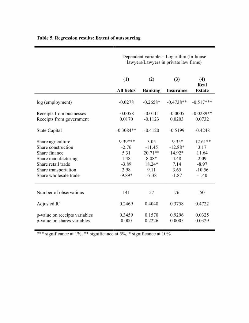
Table 5. Regression results: Extent of outsourcing

Dependent variable = Logarithm (In-house lawyers/Lawyers in private law firms)

(1)

All fields

(2)

Banking

(3)

Insurance

(4)

Real Estate

log (employment) -0.0278 -0.2658* -0.4738** -0.517*** Receipts from businesses -0.0058 -0.0111 -0.0005 -0.0289** Receipts from government 0.0170 -0.1123 0.0203 0.0732 State Capital -0.3084** -0.4120 -0.5199 -0.4248 Share agriculture -9.39*** 3.05 -9.35* -12.61** Share construction -2.76 -11.45 -12.88* 3.17 Share finance 5.31 20.71** 14.92* 11.64 Share manufacturing 1.48 8.08* 4.48 2.09 Share retail trade -3.89 18.24* 7.14 -8.97 Share transportation 2.98 9.11 3.65 -10.56 Share wholesale trade

-9.89*

-7.38

-1.87

-1.40

Number of observations

141

57

76

50

Adjusted R2 0.2469 0.4048 0.3758 0.4722 p-value on receipts variables

0.3459

0.1570

0.9296

0.0325

p-value on shares variables

0.000 0.2226 0.0005 0.0329

*** significance at 1%, ** significance at 5%, * significance at 10%.

Table 6. Specification checks: Extent of outsourcing

Dependent variable = Logarithm (In-house lawyers/Lawyers in private law firms)

All fields

Banking

Insurance

Real Estate

Panel 1 Basic Model (Adjusted R2) [Number of observations]

-0.0278 (0.2469)

[141]

-0.2658* (0.4048)

[57]

-0.4738** (0.3758)

[76]

-0.517*** (0.4722)

[50] Panel 2 Two-part model (Bootstrapped standard error) [Number of observations]

-0.4836***

(0.0234) [200]

-0.3761***

(0.0270) [162]

-0.3559***

(0.0236) [162]

-0.3417***

(0.0264) [162]

Panel 3 Dependent variable

Square root (Adjusted R2)

-0.0277* (0.2622)

-0.1185** (0.3433)

-0.2654** (0.4443)

-0.1272** (0.4034)

Identity (Adjusted R2)

-0.0450** (0.2664)

-0.2126* (0.2386)

-0.6954*** (0.4554)

-0.3984* (0.2676)

Panel 4 Market size:

log (population)

-0.0293 -0.2184* -0.4582*** -0.4550***

log (personal income) -0.0331 -0.2279* -0.4744*** -0.4387*** Influential observations

Studentized residuals > 2 (Number of excluded obs.)

0.0537 (5)

-0.1624* (2)

-0.5354** (2)

-0.3939** (1)

Leverage > (2k+2)/n (Number of excluded obs.)

0.0312 (6)

-0.1541* (2)

-0.4646*** (4)

-0.4250** (2)

Cook's D statistic > 4/n (Number of excluded obs.)

0.0649 (11)

-0.2762** (8)

-0.5723*** (6)

-0.4737*** (8)

Median regression

0.0177

-0.2098

-0.5241***

-0.3334*

*** significance at 1%, ** significance at 5%, * significance at 10%. k = number of variables, n = number of observations.

Table 7. Regression results: Structure of law firms

Dependent variable = Logarithm of

(1)

Size

of firms

(2)

Leverage ratio

log (employment) 0.0491*** 0.2251*** Receipts from businesses 0.0073*** 0.0110*** Receipts from government 0.0053 0.0014 State Capital 0.0676 0.1801 Share agriculture and mining -0.8061** 1.1905 Share construction -2.1984** 1.3998 Share finance 0.9384 3.7510 Share manufacturing 0.1090 -0.4953 Share retail trade -0.7241 0.9632 Share transportation 1.4334* 4.9748* Share wholesale trade

0.5449

-5.8553

Number of observations

247

232

Adjusted R2 0.5277 0.3263 p-value on receipts variables

0.0000

0.0397

p-value on shares of employment

0.0005 0.0099

*** significance at 1%, ** significance at 5%, * significance at 10%.

Table 8. Specification checks: Structure of law firms.

Dependent variable:

Size

of firms Leverage

ratio Panel 1 Basic Model (Adjusted R2) [Number of observations]

0.0491*** (0.5277)

[247]

0.2251*** (0.3263)

[231]

Panel 2 Dependent variable

Reciprocal root (Adjusted R2)

-0.0143*** (0.5115)

-0.1819*** (0.2547)

Reciprocal (Adjusted R2)

-0.0169*** (0.4882)

-0.6445** (0.1744)

Panel 3 Market size:

log (population)

0.0362*** 0.2198***

log (personal income) 0.0415*** 0.2111*** Panel 4 Influential observations

Studentized residuals > 2 (Number of excluded obs.)

0.0418*** [11]

0.2443*** [3]

Leverage > (2k+2)/n (Number of excluded obs.)

0.0559*** [16]

0.2053*** [17]

Cook's D statistic > 4/n (Number of excluded obs.)

0.0379*** [18]

0.1841*** [21]

Median regression

0.0595***

0.2185***

*** significance at 1%, ** significance at 5%, * significance at 10%. k = number of variables, n = number of observations.

Table 9. Regression results: Wage inequality

Dependent variable = Logarithm of

(1)

St.Dev. of log

income

(2)

Coefficient of Variation

(3)

Interquartile range

log (employment) 0.0565** 0.0265 0.1126*** Receipts from businesses -0.0002 0.0009 0.0006 Receipts from government 0.0041 0.0018 -0.0012 State Capital -0.0343 0.0262 -0.1277 Share agriculture and mining -0.7924 -1.4277 0.8691 Share construction 0.6655 1.8122 0.3471 Share finance -0.2235 -0.3558 -0.9448 Share manufacturing 0.1623 0.0142 0.4521 Share retail trade 0.7885 0.5186 -0.0059 Share transportation -0.6205 -0.5422 1.5937 Share wholesale trade -1.0333 -0.7845 2.8970 Number of observations

200

200

200

Adjusted R2 0.0561 0.0854 0.1153 p-value on receipts variables

0.7511

0.7930

0.9703

p-value on shares of employment

0.7295 0.1848 0.6237

*** significance at 1%, ** significance at 5%, * significance at 10%.

Table 10. Specification checks: Wage Inequality.

Dependent variable:

St.Dev. of

log income Coefficient

of Variation Interquartile

range Basic Model (Adjusted R2) [Number of observations]

0.0565** (0.0561)

[200]

0.0265 (0.0854)

[200]

0.1126*** (0.1153)

[200] Dependent variable

Square root (Adjusted R2)

0.0199*** (0.0421)

0.0076 (0.0720)

11.5747*** (0.1000)

Identity (Adjusted R2)

0.0272* (0.0310)

0.0072 (0.0607)

4778.51** (0.0921)

Market size:

log (population)

0.0521***

0.0220 0.1036***

log (personal income) 0.0478*** 0.0203 0.0965*** Influential observations

Studentized residuals > 2 (Number of excluded obs.)

0.0838*** [8]

0.0371* [6]

0.1288*** [5]

Leverage > (2k+2)/n (Number of excluded obs.)

0.0357 [11]

0.0142 [9]

0.1094*** [9]

Cook's D statistic > 4/n (Number of excluded obs.)

0.0377* [16]

0.0303* [17]

0.0989*** [13]

Median regression

0.0198

0.0311

0.1128***

*** significance at 1%, ** significance at 5%, * significance at 10%. k = number of variables, n = number of observations.