VOLUME 20,MUMBLER

Our .know. .ec ge oI.' 1:xe Ai:omic Constan):s i. , 1V,m, anc h in .9&:7, anc oI 01:.ter Consi:ants

:3eriva &..e '. .'. ~ereI romJESSE IA . M. DUMOND AND E. RICHARD COHEN

California Institute of Technology, Pasadena, California

I. INTRODUCTION

A. Object and Scope

"ANY critical reviews of the natural eon-- ' stants and conversion factors of physics

have appeared in the last thirty years. Themonumental work of R. T. Birge' in manypapers published during this long period is out-standing in the field for its thoroughness andpainstaking critical attention to every conceiv-able detail and to every source of information.Many other excellent studies have been madeby a number of competent physicists dealingwith this subject. There would be but little ex-cuse for further contributions were it not for thefact that with the passage of time the situationbecomes considerably modified (1) owing tonew experiments and improvements in experi-mental techniques and (2) because of thebroadening of our knowledge.

The present paper aims to deal only with alimited portion of the subject, the evaluation ofthe so-called atomic constants: e the electroniccharge, m the electronic mass, and h Planck'sconstant of action together with certain auxiliaryconstants intimately associated with them. Anumber of useful physical constants which canbe computed from the above data will also beevaluated.

The atomic constants e, m, and h have beenevaluated by means of many experiments which,

' The authors are deeply indebted to Dr. Birge for helpand criticism over a long period. They have relied exten-sively on his published work and his generous extensiveprivate communications. A very abbreviated list of hismore important published papers follows: R. T. Birge,Rev. Mod. Phys. 1, 1 (1929); Phys. Rev. 40, 207 (1932);Phys. Rev. 40, 228 (1932); Phys. Rev. 42, 736 (1932);Nature 133, 648 (1934); Nature 134, 771 (1934); Phys.Rev. 48, 918 (1935); Nature 13'7, 187 (1936); Phys. Rev.54, 972 (1938); km. Phys. Teacher 7, 351 (1939); Phys.Rev. 55, 1119 (1939); Phys. Rev. 57, 250 (1940); Phys.Rev. 58, 658 (1940); Phys. Rev. 60, 766 (1941); Reportson Progress in Ph sics, London, VIII, 90 (1942); Am. J.Phys. 13, 63 (1945 .

in general, measure some function of one, two, orall three quantities, together mith auxiliary con-stants. In this process one obtains more equationsthan the number of unknowns and a certainamount of overdetermination thus results whichpermits us to discuss the consistency of the dif-ferent determinations with each other. Over thelong period during which the subject has beeninteresting to physicists this situation has ledto a series of "discrepancies" each of a di8'erentnature, which, one after another, have beenmore or less resolved by further research and byimprovements in the measuring techniques. Be-cause of the entangled nature of the primarydata each discrepancy, before its true cause hadbeen located, appeared to offer a very compli-cated series of possibilities threatening extremelyramified modifications in the entire picture.Thus, for example, there was, at one time, muchdiscussion of the "e discrepancy. "This appearedas a difference between the supposed "oil drop"value of e and the value computed from theFaraday Ii and Avogadro's number' X when thelatter is determined by absolute length measure-ments of the atomic lattice dimension of crystalsusing x-ray wave-lengths standardized with ruledgratings. The discrepancy was resolved whenthe values originally used for the viscosity ofair, in reducing the data from the oil drop ex-periment, were shown to be in error. Before thiserror was found, however, many other possi-bilities were explored and eliminated, some ofwhich would have had very far reaching conse-quences if they had been true.

Another discrepancy which has occupied muchattention and which is not yet completely re-solved concerns the values of e/nt as determined

' We have endeavored to adhere as far as possible to theexcellent nomenclature of Birge. Avogadro's number whichBirge calls No we designate simply by N so that we canreserve the subscript zero to indicate what we call ourconventional adopted origin values of the unknowns.

ATOMIC CONSTANTS

on the one hand by spectroscopic measurementsand on the other hand by measurements in-

volving deRections of electron beams by meansof applied electric and magnetic fields.

Still a third discrepancy has lately attractedattention. This may be described by stating thatthe observed values of Ii/e (as measured by ex-periments on the quantum limit of the continu-ous x-ray spectrum) yielded significantly lowervalues than were obtained by computation fromthe best measured values of e, e/nz, and theRydberg constant, R„=2x'me4& —'c—'. Both ana-lytical and graphical examinations of the entiremass of data including the results of many othermeasured functions of e, m, and h have led

rather definitely to the conclusion' that thetrouble lay with the measured x-ray values ofb/e. These measurements have therefore re-

cently been repeated by two different groups ofworkers' in the United States and in Swedenin quite different regions of the x-ray spectrumwith most interesting results which not onlyindicate that this discrepancy has been prac-tically eliminated but which also reveal thereasons for many of the earlier "low" experi-mental values of It/e. These new results opensome new questions regarding minor correctionsto the measured x-ray value of b/e which areunfortunately not yet completely resolved butwhich introduce, in the case of the Americanmeasurements, corrections only of the sameorder as the estimated probable error of themeasurements themselves. They are, therefore,chieQy of theoretical interest at present. Thesituation regarding tt/e is therefore' far moresatisfactory than it has ever been in the pastfor we are now in a position to reject, for goodand sufficient reason, all earlier measured b/evalues which were significantly "low, " and wepossess one measured Ii/e value which, as weshall show, can be justifiably incorporated alongwith nine other independent measured func-tions of e, m, and k into a least squares solution

3 F. G. Dunnington, Rev. Mod. Phys. 11, 65 (1939);J. W. M. DuMond, Phys. Rev. 56, 153 (1939) and Phys.Rev. 58, 457 (1940); F. Kirchner, Ergebnisse der ExaktenNaturwiss. 18, 26 (1939).

4W. K. H. Panofsky, A. E. S. Green, and J. W. M.DuMond, Phys. Rev. 62, 214 (1942); Per Ohlin, Disserta-tion, Uppsala (1941);Arkiv. f. Mat. Astr. och Fysik 27B,No. 10; 29A, No. 3; 298, No. 4; 31A, No. 9; 33A, No. 23.

for the "best" values of those constants in thelight of present knowledge.

This is one new element in the situation, thediscussion of which is one of the justificationsfor the present paper. The other new elementconcerns a new viewpoint as regards the un-knowns to be determined by least squares ad-

justment.It must be admitted that the results sti11

contain minor uncertainties which make it neces-sary to regard the persent numerical values asprovisional only. Further clarification of certaindetails in the b/e work with x-rays may a littlelater permit inclusion of the Uppsala values andmay thus greatly improve the accuracy withwhich h/e is known. The situation regarding thee/m discrepancy may yet be still somewhat im-

proved. The slight discrepancy between theiodine and silver values of the Faraday may beresolved in the future. To postpone the presentpaper until any or all such minor matters arecleared up would be unfortunate since it mightinvolve a delay of several years. As E. U. Condonhas pointed out, there is a definite value in ascertaining and adopting generally acceptable standardvalues for the constants of pbysics at strategicallychosen times, even though these vulles are ad-mittedly provisional, since, by so doing, a desirableuniformity and consistency of usage in the literature is obtained. In the judgment of the authorsthe present situation is sufficiently satisfactoryto warrant such a provisional set of values andone of the purposes' of this paper is to presentthe evidence for this judgment.

It is this need for a standardized set of values,even though they be provisional, which is theonly justification for the weighted averaging andleast squares adjustments typical of the presentpaper. As H. A. Kramers has very aptly put it,"The theory of least squares is like love—onecross word can spoil it all. " The procedure of

~ In 1940 a continuing committee of the NationalResearch Council known as the "Committee on Funda-mental Constants and Conversion Factors" was formedunder the chairmanship of Dr. L. J. Briggs as a jointcommittee under the N. R. C. Divisions of Chemistry andPhysics with the stated purpose of ascertaining andpublishing from time to time the best and most generallyacceptable values of the physical constants. Responsibilityfor the subdivision of the atomic constants was assignedto one of the authors of the present paper and its contentstherefore constitute a report to the above mentionedcommittee.

J. hV. M. D IJ5tlON D AN D E. R. COHEN

YAM.E IA. Experimental sources of information in determining e, m, and k. "Old" or traditional viewpoint.

Description of experiment Quantity determined Numerical value

Function ofe, m, and hdetermined

Auxiliary constantsinvolved

1. Spectroscopic determinations of the Rydbergwave number equated to Bohr's formula.

2. Direct determinations of e by the ruled gratingand crystal x-ray Inethod.

3. Specific charge of the electron (spectroscopicmethods, deQection methods or other).

4. Measurements of the quantum limit of the con-tinuous x-ray spectrum.

5. Electron diffraction measurements of DeBrogliewave-lengths for electrons accelerated with ameasured voltage.

6. X-ray photoelectrons ejected with known quan-tum energies, hv, and measured by magneticdeflection.

7. Determinations of fine structure constant a.8. DeBroglie wave-length by electron diBraction in

which the speed of the electrons is measured kine-matically. Compton shift measurements.

Ai ~2mmmc4h 3c i =R~ R~ ~109737.3 me4h~ c

A I =-t./m

A4 -h/e

A g =h/(em)&

c =4.80193 )(20 io

g/m ~1.75903 +10't

h/e =1.3786 X20» he i

F;NMc @g(),[2dspy(P)]

I/ SPI q~

p; q; c; 4/~, s

A g =e'/(mh) c~/(mh) =3..8197 &1Q~ em &h+ Pg/X8; c

A7 =2me2/(hc) =aAs =h/m

A se =h/m =c'Ag

a =(136.95)-ih/m =7267

h/m =7.255

c~/h

h/m Xg/Xg

h/m Q/P g; c

h/(em}~ ~l.00084+10 s he '~m & p; q; Xz/X,q~

Velocity of lightc ~(2.99776~0.00004) &(10&o cm sec.-&

Avogadro's number~+N = (6.02338~0.00043) )(2023 mol i (chemical scale)

Atomic weight of calciteMc Co =100.091~0.005 (chemical scale)

Density of calcite p =2.71029~0.00003 g cm ~

Calcite volume factor rp(P) =1.09594~0.00002

Conversion from Siegbahn to absolute wave-lengthsXg/Xg ~1.002030~0.000020

Grating space of calcitedao = (3.03567&0.00005) )(10 I cm

Faraday**F =9648.5 ~1.0 e.m.u. equiv. i (chemical scale)

Conversion from NBS international electrical units toabsolute units

1 NBS ohm = P absolute ohm p =1.0004951 NBS volt =pq absolute volt pq=1.0003301 NBS ampere = q absolute ampere q ~0.999835

Atomic weights (physical scale)H 1.008131~0.000003D 2.014725 ~0.000006He 4.003860~0.000031

Gas constant per mole.Ro =(8.31436~0.00038) )&20~ erg mol i deg. i

Volume of perfect gas (O'C)Vp =(22.4146~0.0006) X203 cm' atmos. mol i

Source*

Birge

Birge

Birge

Birge

Birge

Birge

Birge

Recalculated

NBSNBSNBS

MattauchMattauchMattauch

Birge

Birge

+ Birge: R. T. Birge, Reports on Progress in Physics (2941), PhysicalSociety, London (1942). NBS: National Bureau of Standards, privatecommunication (see text). Mattauch: J. Mattauch, Nuclear PhysicsTables (Interscience Publishers, Inc., New York, 1946).

++ The values of the Faraday and Avogadro's number given hereare the obsemed values and not the least square adjusted values ofTable VIII. The latter are to be considered as the "best values. *' SeeBirge, Am. J. Phys. 13, 63 (1945).

obtaining adjusted values by weighted averagesof many different experiments (whose disagree-ments are most probably in part the result ofunknown systematic errors) has been severelycriticized in many quarters. The school ofthought which opposes such a procedure has nobetter alternative to offer, however, than to

TAM.E IB.Directly observed values of auxiliary constants.

wait hopefully for still better experimental re-sults and, in the meanwhile, to be completelynoncommital as to adoption of values .The prac-tical result of this, however, is a woeful lack ofuniformity in the literature since writers are con-tinually obliged to make calculations involvingthe constants.

There is really no danger in the use of sta-tistical theory for the calculation of adjustedvalues of the physical constants with their re-sulting probable errors, provuied we do not forget the provisional character of the results If.unknown systematic errors are presen, t in theoriginal data, we can only hope that, with asufhcient number of independent experiments,even the systematic errors will tend to have arandom distribution. Since we must determineprovisional values from a supply of partially in-consistent data, the most convenient tool me have

is a least squares adjustment. It furnishes an im-partial analytic method of determining a set ofcompromise values which do the least possibleviolence to a11 our sources of information.

B. The Experimental Sources of Information

The experiments which yielded the data usedin the present paper have usually been classifiedinto eight types, each of which determines adiferent function of the variables e, m, h. InTable IA we list these in the order of decreasingprecision and reliability giving, the function de-termined, a description of the (one or more)

ATOM I C CONSTANTS

experiments which determine it, and the nu-merical value A; at present adopted for eachfunction together with its probable error asestimated from the determining experiment orexperiments. Certain auxiliary constants are alsoneeded in each determination and these are alsolisted in the formulae, Table IA. Their defini-tions and adopted values are given in Table IB.In the computation of some of the derived con-stants at the end of this paper a few additionalauxiliary constants are needed and these, forcompleteness, are also listed in Table IB. Insucceeding sections we shall discuss the sourcesof all these data and our reasons for the adoptedvalues and precision measures.

C. The Entangled Nature of the Data

R. T. Birge has justly pointed out that in theanalysis of data such as we must deal with hereit is extremely important (1) to distinguish theprimary data of experiment from derived dataand (2) to ascertain clearly just what functionof the unknowns each experimentally deter-mined numeric really stands for. Constants suchas R„or c whose relative error is very small incomparison to the majority of the unknowns

can, of course, be treated as accurately deter-mined numbers. This is not true, however, of a11

the auxiliary constants and, as we shall presentlysee, the Faraday F and Avogadro's number Xareparticularly important cases of primary datawhich should be allowed independent freedom ofadjustment in a least squares compromise solu-tion. In the past it has been customary to intro-duce the quotient Jr/N= e, the electronic charge,as a singte primary datum. However, F and Xappear separately and in diferent ways in theformulae for the determination of constantsother than e that form, in some instances, partof our primary data and, in other cases, data tobe derived. Therefore, the only strictly logicalprocedure is to treat F and 1V as independentunknowns. The electronic charge e then has thestatus of a derived constant. Although both 1&

and N have each been determined by experi-ment, there is no guarantee that the adjustedvalues of these constants resulting from a leastsquares compromise solution of the overdeter-mined set of equations in which they are involvedwill be exactly equal to the original directlyobserved experimental values of Ii and N.

The adoption of this new viewpoint consti-tutes the second important new element in the

T&81.E II. Experimental sources of' information in determining Il, N, m, and h. New viewpoint.

Description of experiment

1. Spectroscopic determinations of Ryd-berg wave number equated to Bohr'sformula.

2. Direct determinations of Avogadro'snumber by ruled grating and crystalx-ray method.

3. Direct determinations of the Faraday(silver and iodine voltameters).

4. Atomic weight of the electron by spec-troscopy.

5. Specific charge of the electron by deflec-tion methods and Zeeman effect.

Quantity determined

A i =2~2me4h 2c i =R

Numerical value

R =109737.3

A4=mV

F =9648.5

¹n=5.48541 X10 4

A» =e/m e/m =1.75920 X107

A2 =Mcaco» t2d'pq (p)) =N Ã =6 02338 )&10" ~caco», & t . v (P)

Nm

FN-im i P, q;c

Function of F,N, m, and h Auxiliary constantsdetermined involved

F4N 4mh-2

6. F(e/m) from Bearden's x-ray refractiveindex of diamond.

7. Measurements of quantum limit of con-tinuous x-ray spectrum.

8. Electron diffraction measurements ofDeBroglie wave-lengths for electrorisaccelerated with a measured voltage.

9. X-ray photoelectrons ejected withknown quantum energies, hv, and meas-ured by magnetic deflection.

10. Determinations of fine structure con-stant n.

11. DeBroglie wave-length by electron dif-fraction in which the speed of theelectron is measured kinematically.Compton shift measurements.

A» =F(e/m)

A7 =h/ei

+8 =h/(Cltl)~

A =e2/(mh)

A io 2me2/(hc) ~a

Aii =h/m

Aiic =h/m =cXc

P(e/m) =1.69870)&10u F2N im i

h/e =1.3786 X10» P iNh P. e; C, &c/)~

C2/(mh) 3.8197 X1034 I 2N 2&&t ih i 'Ag/W, q, c

n =(136.95) i +2N 2h i

h/m 7.267

h/m =7255 m ih )tt/Xg; c

h/(cm)& =1,00084 X1.0» F-&N~ttt &h p, q; g~/p, ,q

J. W. M. DUMOND AN D E. R. COHEN

present analysis. It leads to the adoption ofTable II for the description of our primarysources of information. Under the new viewpointthe chief changes are three in number:

(1) Two unknowns, F and N, are introducedin place of the one unknown, e.

(2) Three quite different and independenttypes of experiment, all of which have in thepast traditionally been regarded as determininge/m, on the new viewpoint now fall into threeseparate classes: (a) spectroscopic experiments(such as those on the II and D lines) which

really determine the atomic mass of the electron;

(b) "deflection" experiments which are legiti-mate determinations of e/m; and (c) Bearden'smeasurement of the refractive index of diamondfor x-rays which really measures the productP(e/m).

(3) The ruled grating and crystal x-ray de-terminations traditionally regarded as deter-minations of e are now classified as what theyreally are, direct determinations of Avogadro'snumber X.

In the application of the new viewpoint theauxiliary constants used are still those of TableIB. We must however distinguish the directlyobserved F and N of that table from the finaladjusted values of these constants which weshall receive as the result of all least squaresadjustments. (Actually it turns out thatsuffers very little change from the directly ob-served value, but this could hardly have beenpredicted. )

Because this new viewpoint represents a con-siderable break with tradition, we have thoughtit wise to work the entire problem through byboth methods so that the results can be compared.We shall distinguish the two methods merelyby the adjectives "old" or "traditional" on theone hand and the adjective "new" on the otherhand. We believe the results by the new methodare those that should be recommended for tem-porary adoption simply because they do lessviolence to all of the known data with appro-priate weighting.

It should be pointed out that it is the whole-hearted espousal of the principle of least squaresadjustment in the present work which forces usto the adoption of the new viewpoint. In thepast the usual procedure was to apply the prin-

cip1e of least squares merely to finding the bestrepresentative value of each directly measuredquantity (a weighted average value of R„, forexample, or a weighted average value of Ji).Then a definite path was selected for computingeach derived constant utile'ing the most accuratePrimary data as the criterion for selection of thepath. This path was as follows: combining Fand N one obtained e. Then combining e=F/2Vwith the best adjusted mean value of e/m andwith R.„=27r'me4h 'c ' one solved the threeequations for e, m, and h. In computing otherderived constants one took pains always to ex-press them in terms of the primary data (e/m,R„, e). Other paths for arriving at the resultscould conceivably have been used (taking anexample at random) such as to combine e = F/1Vwith the observed value of 0. =2xe'h 'c ' andR„=2m'me4h 'c—' to solve for e, m, and h. Sucha possible path was not used for the obviousreason that it was much less accurate because ofthe relatively large uncertainty in the deter-mination of 0.. A simple enumeration shows thateven if R„ is always included as one of the data,there are still some 15 different paths by whichone could evaluate the atomic constants. Toselect the most accurate path, however, amountsto attaching zero weight to a great deal of in-formation and the present situation as regardsconsistency seems suKciently satisfactory (as weshall endeavor to show below) to warrant a moreinclusive procedure.

When we make a least squares adjustment ofall the data, however, we have abandoned thechoice of any specific path. We must first decidewhat we shall consider as fixed constants andwhat shall be regarded as unknowns. Let U bethe number of unknowns. Then we write downall equations in which experimentally deter-mined functions of these constants and un-knowns are equated to the numerical valueswhich the experiments yielded. The number ofthese equations, E, considerably exceeds thenumber U of unknowns and the equations arenot exactly compatible, but the theory of leastsquares teaches a definite procedure for findingcompromise values of the unknowns which dothe least possible violence to each of the de-terminations, taking due account of the relativeweights which we attribute to each equation in

ATOM I C CONSTANTS

view of its estimated probable error. The 6naladjusted values of the unknowns will differslightly from those arrived at by any particularpath in which some selected set consisting ofonly U of the total of 8 equations was used.

Our least squares adjustment procedure underthe old viewpoint is to select as unknownse(=F//r/), m, and h and to classify F and Kamong the 6xed constants. The application ofthe principle of least squares then to the nine'equations represented in column 2 of Table IAleads us to adjusted values of e, m, and h. Butthe adjusted value of e turns Oui Io be not quiteequal to the quotient of the constants I' and E initially inserted If we i.ndicate final adjusted valuesby bold faced type, the results are as follows

Inserted value

F=9648.5 +1.0 e.m. u. (chemical scale).

lV= (6.02338&0.00043) X10";cF/N=s=(4. 80193+0.0006) X10 "e.s.u.

Adjusted value

cF/N = e = (4.80214a0.00047) X 10—"e.s.u.

'Equation (1) for R„ is so accurate (i.e., deserves somuch weight) that it can merely be used to eliminate oneof the unknowns from all the others before applying theprinciple of least squares. Equations (7), (8), and (8c) allessentially determine h/m since c is known with sufficientaccuracy to regard it as a fixed constant. There are there-fore really six independent equations for the adjustmentof two unknowns.

7 Throughout this paper we indicate the accuracy withwhich a quantity is known by quoting the figure 0.67450.The standard deviation, 0, of the mean of N weightedobservations is given by

a' =ZP;s -/(rV —1)ZP;

where p; are the weights assigned to each observation andv; are the deviations of each observation from the weightedmean of the set. The range of the number such that theprobability is 0.5 that the correct value lies within thatrange is called the probable error (I'Z). It is well knownthat for observations that have a Gaussian distributionabout the mean value, PB=0.6745'.. In the general theoryof the least squares fitting of several variables, the standarddeviation of each variable can be defined in a definitemanner which involves only the observed quantities andis independent of any detailed assumptions as to thenature of the distribution from which the data were taken.The probable error on the other hand is more dificult todetermine and requires a knowledge or at least an assump-tion of the form of the distribution functions. However,since the quantity usually used by physicists is the probableerror, we have defined, somewhat loosely and arbitrarily,the probable error to be PE=0.6745o and quote thisvalue although the standard deviation o. is the quantitywhich actually results from our analysis.

The question then immediately crises as to whattve shall cull our sePurate adjusted values of F andN since the adjustment under the old viewpointhas only given us an adjusted value for their ratio.The conclusion that our adjustment under theold viewpoint did not provide a sufhcient num-ber of degrees of freedom is thus forced home. Itbecomes even more acutely evident when wemust compute derived constants from our ad-justed values of e, m, and h. Many of theseinvolve Ii and X not only implicitly in the vari-able e but also explicitly in such a way thatthey cannot be expressed as functions of F/Kalone. To be consistent we nrusI decide on sepa-rate adjusted values F and N to use in thecomputation of these derived constants. There-fore, in our procedure under the old viewpointwe have adopted the quite arbitrary method ofdetermining F and N by adjusting the relativedeviations [ F—F

~/F and [ N —X[/X so as to

make these directly proportional to the squaresof the probable errors (inversely proportional tothe weights) of the direct determinations of Fand X, respectively, while imposing the furthercondition that F/N shall equal our adjustedvalue of e. By so doing we have departed fromthe thoroughgoing application of the leastsquares principle because, for example, some ofour other determinations, notably those usuallyclassified as determinations of e/m, contain im-

plicit information regarding F to which someweight should be attached. This is why we can-not recommend the old viewpoint values.

To summarize we may say that the old view-point assumes three unknowns, say e, m, and h,which number can be reduced to two by theapplication of the Rydberg relation, while thenew viewpoint assumes four unknowns Ii, N,m, and k equivalent to three after applicationof the Rydberg relation. The larger number ofvariables under the new method introduces anunavoidable difficulty in depicting the situationgraphically.

D. Graphical Representations to Depict theInterconsistency of the Data

In the analysis of such complicated situationsas the present one, graphical aids are of greatutility in forming judgments even though theymay not be used to obtain numerical results. In

88

th. ls connection the Blrge-Bond diagram, as it 18

called, has rendered very valuable service. Toconstruct such a diagram one particular un-

known, such as e, is selected for plotting. R. T.Birge has described in detail the construction ofsuch diagrams, and the reader is referred to his1932 article for the description. Birge more re-cently plots scales on the ordinates which readdirectly in terms of the function to which eachcorresponds. In the latest diagram of this typeBirge selected the two ordinates representing (1)the "direct" determination of e (from F and thex-ray determination of Ã), and (2) the bestaverage of all e/m determinations (some of whichlllvolve F and soIlle of wlllcll do llot) Gs Llà 48-

termining orCinates for drawing his straight line.He states that a least squares adjustment wouldlead to substantially the same results as thisline yields. The data then available, especiallywhen represented in this way, certainly did notseem to warrant such an adjustment because ofthe II/e discrepancy and the rather weak weightsthat would have been attached to all data save eand e/m on his chart.

For our present discussion we prefer to utilizea diferent kind of graphical representation de-veloped some years ago by one of us' because itlends itself somewhat more readily to the kindof thinking which our present method of leastsquares adjustments requires. This graph whichwas originally called an "Isometric ConsistencyChart" was designed from the old viewpoint re-

garding e, m, and h as the unknowns and we shallexplain it in these terms. We wish it clearlyunderstood that this chart has never been andis not now intended as a nomogram for arrivingat adjusted best values. It is merely a way ofdepicting the interconsistency of input data witheach other and with the adjusted value arrivedat by least squares computations. It also offers aconvenient method of exhibiting the "ellipse oferror.

Consider a three-dimensional space in whichthe values of the three unknowns e, m, and h

' See R. T. Birge, "The general physical constants as ofAugust 1941 with details on the velocity of light only,

"Reports on Progress in Physics 8, 124 (1942}. For adescription of the construction of the Birge-Bond diagramsee R. T. Birge, Phys. Rev. 40, 22& (1932) and, in partic-ular, pages 232-5 and 252.' J.W. M. DIIMolld, Phys. Rev. 56, 153 (1939);58, 457(1940).

appear plotted on mutually rectangular car-tesian coordinate axes. To each point in thespace there corresponds a triplet of values, e,m, h. Each equation of column 2, Table IA,defines a surface in this space. These surfacesall very nearly pass through a common point.In this region of quasi-intersection a slightchange in the experimentally determined con-stants A; of these equations will displace thecorresponding surface in the direction of itsnormal. It turns out that the relative changes inthe A's needed to bring all surfaces into coin-cidence at a single point are all less than 0.5percent and indeed most are of order 0.1 percent.Only negligible second-order errors, therefore,are introduced if we replace the surfaces (whichare, in general, curved) by planes tangent tothese surfaces in the region in question. It thenbecomes our object to study these variouslytilted planes in the region where they nearlyintersect in a common point. tA'e can think of theleast squares solution as an analytic method ofselecting a point in this space in such a wa~

that the sum of the weighted squares of itsrelative distances from all of the planes shall beminimized. The weights, according to the theoryof least squares, are to be adjusted so as to beinversely proportional to the squares of the esti-mated probable errors of each determined A, .The thought behind this procedure is, of course,that each such weighted plane represents a smallsample out of a much larger universe of observa-tions which, if they had all been made, wouldhave yielded Gaussian distributions for the posi-tions of all planes whose centers would all havepassed consistently through a common pointof the space. This is an assumption, nothingmore, but in the absence of better informationit is about the best we can do. A further conse-quence of this assumption is that there exists inthis space an "ellipsoid of error" defined by thedifferent Gaussian distributions of the planes.VA shall discuss this a little later.

It is desirable to eliminate dimensional con-siderations from our problem and therefore ourprocedure is to select an origin point eo, mo, ho in

the e, m, h space whose relative distance fromeach of the planes shall be small and to definenew dimensionless variables x, =(e—ep)/ep, x= (m mp)/mp, x@= (II —Ap)/hp, the relative de-

ATOM I C CONSTANTS

viations of our original unl-nowns from the arbi-trary origin values, all of which, it turns out, area small fraction of one percent. In terms of thesenew variables each of our experimental equationsof type

4Ã,,+ x~ —3xg = ci

Xo X$8

—x1——x 6

2x;2x.

1—j»~+ &a =os&ri. = a6

XI =ava8

Relative Weights

65I31230.97.3

(8) 0.7; (Sc) 0.1.

(3)

The subscripts of the o, s correspond to the nuiu-bering in column 2 of Table IA. The first of theabove eight equations which corresponds to theRydberg relationship must be given so muchmore weight than any of the others because ofits high accuracy that, in practice, the bestprocedure is to eliminate one of the variablesfrom the entire set by means of it before pro-ceeding to the least squares adjustment.

At this point let us examine how our eight.tangent planes look in the x„x„„x~,space. Firstlet us consider only their orientations. For thispurpose we can set the a's all equal to zero sincethis merely shifts each plane in the direction of

becomes a linear equation of type

&&e+g&m+lt&h=ctijkq

wherein each a is defined as a=(A —Ao)/Ao.Here A p is the origin value of A, that is to say,

A p= 8p f@p~kp

The approxima, te Eq. (1), which is the equa-tion of the tangent p'lane to each observed sur-face in our space of relative deviation from thearbitrary origin, neglects second-order terms in

the binomial expansions which are of order onepart per million since the variables are of order0.1 percent. Our problem is thus linearized, andwe now have a set of eight di6'erent linear equa-tions of the type of (1) in three unknowns whichare not exactly compatible and which are to beadjusted by the standard procedure of leastsquares. These equations take the following form:

its normal. The coefficients of the variables inthe eight equations (3) above form a matrixcharacterized by certain properties which areinvariant to any transformation of axes and are,therefore, of fundamental importance in under-standing the situation. From this matrix of eightrows and three columns, 6fty-six different third-order determinants can be formed and tnrelvs ofthese determinonts vonisk. Geometrically, each of,these means that the corresponding set of threeplanes contains a common axis in the space. Sucha set of three planes constitutes a degeneratecase which defines a line but which is incapableof locating a point in the space. If the a's arenot zero this means for such a degenerate casethat the three planes are parallel to a commonline, though they may not pass through it. Nowit turns out that, out of our present set of eightplanes, actual/y Pre of them are parallel to a com-

mon line. These are the ones numbered 3, 4, 5,6, and 8. This line makes equal angles with thethree axes x„x, xz. The matrix defines onlytwo other axes to which more than two planesare parallel, but neither of them is associatedwith as many planes as this one." Adopting aterm frorri crystal structure we shall speak ofplanes which are parallel to a common axis asbelonging to a "zone" and such a set of planeswill be described as a "cozonal" set. If we thinkof the positive octant of our x„x,„, x~, space,then the Ave planes are parallel to and verynearly contain a line through the origin makingequa1 acute angles with the three positive axes.If we look at the planes along this direction, weshall see all hve of them on edge. There remainonly three planes, (1) the .R„plane, (2) the o

plane, and. (7) the e'/tt plane determined by thevalue of the hne structure constant n. The lastof these is considerably less accurately knowiithan the 6.rst two. One way of stating the situa-tion, then, is that five of our eight equations areonly capable of dehning ~atios between the con-stants e, m, and h. This drives home forcefullythe extreme responsibility of the first two of ourequations in. determining the three unknownconstants e, m, and h. Once the position in spaceof a best Iitting cozonal axis has been established

"A complete enumeration of all such axes is given in aprevious paper, J. Ml. M. DuMond, Phys. Rev. 58, 459(1940), see Fig. 1.

J. W. M. D UMON D AN D E. R. COHEN

for the five cozonal planes, the remaining twoplanes may or may not intersect this axis in thesame point. " In this respect the overdetermina-tion is evidently not as high as it could havebeen in the case of a less degenerate matrix. Itis, therefore, very fortunate that the two planesin question happen to represent the two mostaccurate determinations of all.

Because of this particular degenerate peculi-arity of the set the isometric consistency chartwas constructed as a view projected on the (111)plane of the x„x, xy, space of the five cozonalplanes (seen on edge) which therefore appear aslines on the chart. Each line is provided with itsown scales, normal thereto, giving displace-ments of that line corresponding to diferentpositive or negative percent deviations of thefunction in question from the origin value of thatfunction. In order to represent on the two-dimensional diagram the non-cozonal planes (2)and (7), recourse is had to the Rydberg relationwhich is considered to be essentially exact.Geometrically, this amounts to finding the linesof intersection of planes (2) and (7) with theRydberg plane and projecting each of these linesin space on the (111)plane of our isometric chart.(The reason for the name "isometric" is nowobvious. It is borrowed from drafting termin-ology. ) Any axis determined by the cozonalplanes will be seen end-on and will appear as apoint on this chart. If either the plane (2) (directdetermination of e) or the plane (7) (determina-tion of n) cuts this axis at the same point as the8 plane (1), then the projected intersection linefor that non-cozonal plane will, on our chart,pass through the point. Scales are also pro-vided to show displacements of the non-cozonallines calibrated in percent deviation of the corre-sponding functions from their origin values. Itis furthermore easy in the same way to providedisplacement scales for lines corresponding toany function of the three variables e, m, h

whether they belong to the isometric zone ornot and, in particular, it is convenient to providescales for m and h on the chart. To every pointon the chart, therefore, there corresponds a valueof e, m„and h whose percentage deviation fromthe origin values eo, mo, ho can be read oiY di-

"The spacial appearance has been shown in a perspec-&jve view, Phys. Rev. 56, 156 (1939),Figs. 1 and 2,

rectly on the appropriate scales. To distinguishscales for the non-cozonal variables from therest, two lines are drawn along the lengths ofthese while one line only is drawn along thedivisions for cozonal scales.

Figure 1 shows on our isometric consistencychart the experimental data of Table IA. Theleast squares adjustment of these data yields thepoint indicated by a small white circle at thecenter of the black ellipse. This point showsgraphically the best adjusted values of e, m, hand functions thereof under the old viewpointaccording to which these three are regarded asthe primary unknowns. These results which me

do not recommend together with a few of the de-rived constants are listed numerically later inthis article for comparison with our recom-mended values.

Examination of this chart permits us to forma judgment regarding (1) the general consistencyof the input data, (2) their estimated (input)probable errors (which are represented by twolines equally and appropriately spaced on eitherside of the center line for each variable), (3) thedeviation of each input datum from the adjustedbest value, and (4) the probable errors of theadjusted best values of e, m, and h and functionsthereof. The probable error of the adjusted bestvalue of e, m, h or any function thereof is givenby the width of the black error ellipse projectedon the scale for the variable or function whose

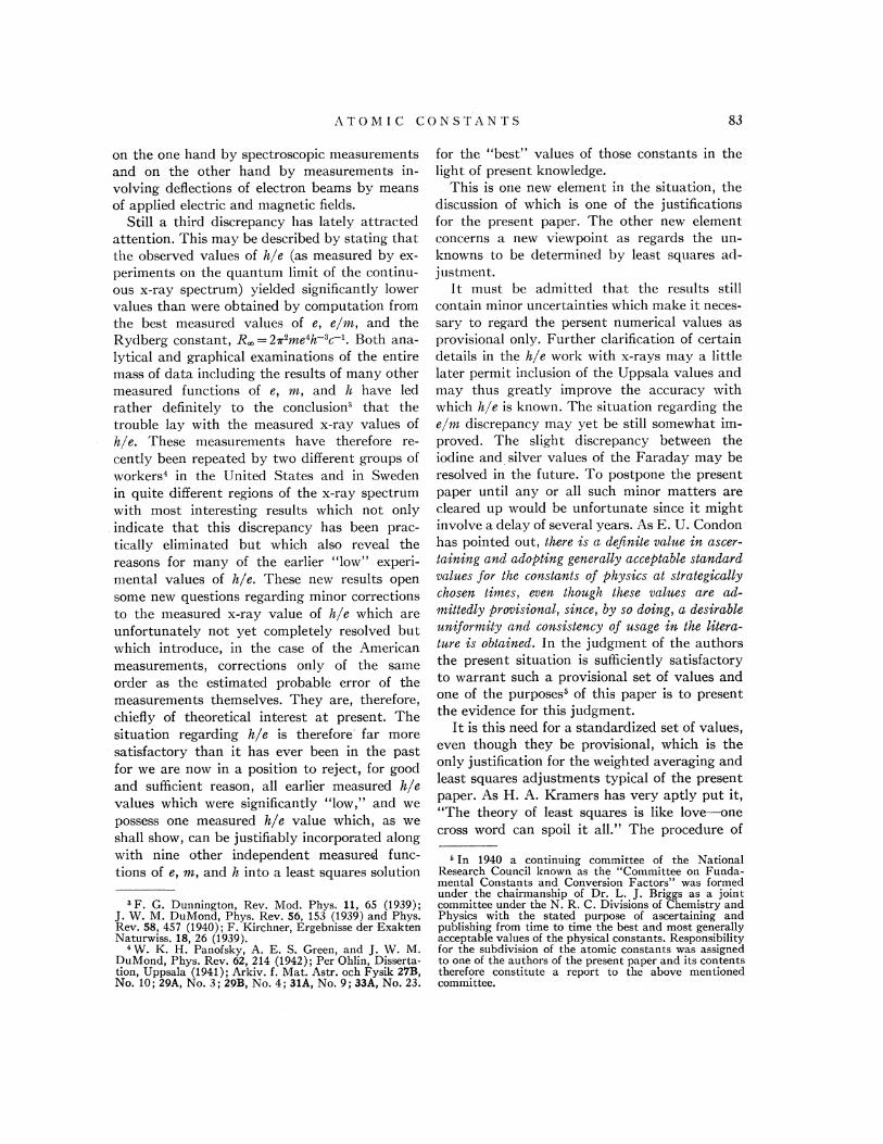
probable error is desired. In order to exhibit thissituation more clearly we show in Fig. 2 this errorellipse to nxuch larger scale than in Fig. I. Theprobable error spread of each variable or func-tion is emphasized with a heavy black strokealong the corresponding scale. This brings us

quite naturally to a discussion of the determina-tion of the precision measures for the adjustedvalues of variables and functions thereof re-sulting from such a least squares adjustment asours.

E. The Problem of EstimatingPrecision Measures

Probably the most important new conceptwhich is introduced regarding the calculation ofprecision measures from a least squares adjust-ment such as the present one is that of the exist-ence of correlation coefficients. We are accus-

ATOM I C CONSTANTS

tomed to the well-known "propagation of errors"formulae for computing the probable error' in afunction of certain variables for each of which aprobable error is given. " What is less obviousand much less generally understood is that suchstraightforward application of the principle ofpropagation of errors leads to correct results if

and only if the input variables are strictly independent (uncorrelctted).

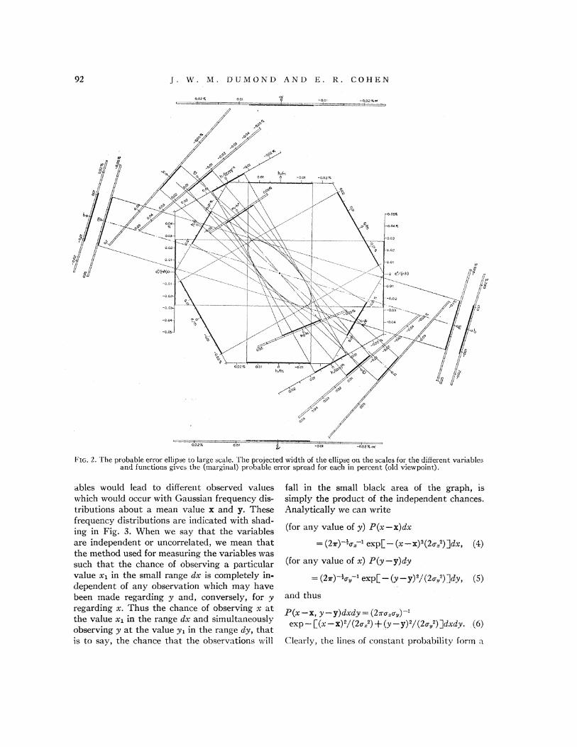
Consider the case of two independent vari-ables, x and y which have standard deviationso. and r„ illustrated in Fig. 3. In accord withthe hypothesis of the theory of least squares weassume that many observations of these vari-

Ot5 0,.4 0,.3O

0,.2 O,t 9 -0tt Wr2 -0,3 -Oi4 +f5

0.5 0.4 0.3 0,2 0.1 "0.2 W.3 QI4 -0.5'Fi

Ftc. 1. Isometric consistency chart showing the experimental input data (Table IA) and the least squares adjustedbest value under the old viewpoint. The adjusted values are given by the white circle in the center of the small blackellipse which latter is the ellipse of probable error. We do not recommend this least squares adjustment under the oldviewpoint, and this chart is shown only for comparison with the results obtained under the new viewpoint (see Figs. 9and 10). The axes of e, m, and h are shown with dot and dash lines. The origin values are given in Section III-A. Thiscut has not been revised to accord with certain small corrections to our numerical values found necessary after the paperhad been submitted. Such changes are wholly unimportant.

"We use the expression "correlation coefficient" for lack of a better word. The quantities F, N, m, and Ig arenot correlated in the strict statistical sense but are observationally related since we do not observe each one independ-ently of the others. The numbers expressing this relationship are mathematically the same as correlation coefficientsas defined, for example, in Kenney, Mathematics of Statistics (D. Van Nostrand Co., Inc. , New York, 1939), Vol. II,Chap. VI. For a discussion of the Law of Propagation of Errors, see g. T. Birge, Am. Phys. Teacher 7, 351 (1939).

VK;. 2. The probable error ellipse to large scale. 1"he projected width of the ellipse oa the scales for the different variable. "and functions gives the (marginao probable error spread for each in percent (old viewpoint).

ables would lead to different observed valueswhich would occur with Gaussian frequency dis-t:ributions about a mean value x and y. Thesefrequency distributions are indicated with shad-ing in Fig. 3. When we say that the variablesare independent or uncorrelated, we mean thatthe method used for measuring the variables wassuch that the chance of observing a particularvalue x» in the small range dx' is completely in-dependent of any observation which may havebeen made regarding y and, conversely, for yregarding x. Thus the chance of observing x atthe value x» in the range dx and simultaneouslyobserving y at the value y» in the range dy, thatis to say, the chance that the observations will

fall in the small black a,rea of the gra.ph, issimply the product of the independent chances.Analytically we can write

(for any value of y) P(x x)dx—= (2x)—'*o .-a exp) —(x —x)'(2o,') $dx, (4)

(for any value of x) P(y —y)dy

=(2~) 'o. '«PL —(y —3)'/(2o. ')ldy (5)

P(x —x, y —y)dxdy=(2so. :o„) '-p-L( —) /(2..')+(y-"y) /(2;) jd.dy (6)

Clearly, the lines of constant probability form q

ATOM I C CONSTANTS

system of similar ellipses in the x, y space withmajor and minor axes paralle1 to the axes of xand y. We can think of a "probability hill, " asit is frequently called, having elliptical contoursfor its horizontal sections and Gaussian dis-tribution curves for all its vertical sections. Theparticular ellipse plotted in Fig. 3 is then theellipse of standard deviation. An ellipse of prob-able error (of dimensions 0.6745 times the oneshown) would contain within it just half thevolume of the hill.

Now let us consider certain varia, bles derived

from x and y, say u=x+y and v=x —y. In Fig.4 the axes of these variables, which make anglesof 45' with those of x and y, are shown, togetherwith the original ellipse of standard deviationfor observations of x and y. In the u, v coordi-nates, however, the principal axes of the ellipseare oblique. This implies the existence of corre-lation coefficients for I and v. At a specifiedvalue of u, say uI, the Gaussian cross sect:ion ofthe probability hill along the line AA has. itsmaximum at M and with variation of ut thismaximum point follows along the oblique locusRR. This line passes through the horizontaltangent points of the ellipse because the ellipseis one of the level contours of the hill. Such alocus is called a regression line. Clearly then,for any specified value of u the most probablevalue of v varies with I, and this is what is meantby saying that u and v are correlated. If we Inuke

no specificatio regarding u, tken eke projectedshape of eke kill on the v axis gives the probabilitydistribution which describes our knowledge of v.

This is called the marginal probability distribu-tion for v. It can be readily shown that the pro-jected widths of the oblique ellipse of standarddeviation on the u and v axes give the respective(marginal) standard deviations o. and 0„ forthese variables in the way indicated in Fig. 4 bythe horizontal and vertical tangents to theellipse. It is not di%cult to show that thesestands. rd deviations can be computed from thestandard deviations for x and y by the simpleapplication of the law of propagation of errorsbut this is only true because x and y are uncorre-lated. This gives us

0. = (o..'+o.„')'* and 0, = (o..'+o„')i. (7)

Since u and v are correlated variables we cannot

compute the standard deviations of functions ofu and v by simple application of the laws of errorpropagation. As a trivial example to drive thisfact home, let us compute the standard deviationin the functions g=(u+v)/2 and Ii=(u —v)/2.The law of error propagation gives:

If (8) were correct, substituting (7) into it: weshould have

But actually & and Ii are nothing but x and yand have, therefore, standard deviations ot =~and o „=a.„so that we see that the ordinary ap-plication of the propagation of errors to thecorrelated variables u and v has led to incorrectresults.

R. T. Birge, in his evaluations of the constants,has been generally careful to avoid the. abovedifhculty by expressing all of his formulae forderived constants directly in terms of his pri-mary observed data which are uncorrelated inmost cases because the measurements were in-dependent in nature. "

When we pass to the case of a least squaresadjustment such as we make in the present

tel+

X=X X=XI X

Fio. 3. Illustrating the two-dimensional elliptical Gaus-sian error distribution function for two independentlyobserved variables, x and y, having standard deviationsa.„and 0.„, respectively. The ellipse of standard deviationis shown. It is one of the contours of the error distribution.

"An outstanding exception to this, however, is the caseof e and e /III which he treats as primary data but whichare correlated because some of the spectroscopic determi-nations which contribute to the weighted average value ofe/III involved F, as did also e. Our present computationsunder the old viewpoint are subject to the same objection.

J. K. Ni. DUMOND AND E. R. COHEN

tional equations:

x = 1.00&0.10y =0.80+0.07

x+2y =3.00&0.07

Weight p,1

2,2

U.= U,p —A—-

0 (7

FIG. 4. The ellipse of standard deviation for two variablesderived from x and y of Fig. 3, namely, u=x+y aridrt=x —y. In contrast to x and y which were independentlyobserved, u and v are correlated in the observational sense.

paper, all variables must be regarded as havingcorrelation coefficients. We make the assumptionthat there exists in the space of our primaryvariables an ellipsoid of error whose principalaxes will lie, in general, oblique to the axes ofany of the variables or their functions. Ourlimited number of weighted observations of thedifferent variables and their functions lead us bystandard least squares procedures to a putativeellipsoid which most nearly expresses the devia-tions of our data from exact precision and con-sistency. This is the higher dimensional analogof fitting a Gaussian distribution in one variableto a limited number of observations of thatvariable.

Suppose that by independent direct observa-tions on two variables x and y we have foundthem to have the values x=1.00~0.10 and y=0.80+0.0'7 and that we have also, by a thirdindependent direct observation, found thatu =x+2y =3.00&0.07. These three observationsare not rigorously consistent. This situation isgraphed in Fig. 5; the three heavy lines repre-senting the input observations do not intersectin a common point. Their input probable errorbands are shown with dashed lines. This situa-tion is expressed by the following set of observa-

the weights being adjusted inversely as thesquares of the input probable errors. The stand-ard procedure of least squares leads to the nor-mal equations for the adjusted values:

3x+ 4y= 7.0,4x+10y = 13.6,

with the solution

x = 1.1143, y =0.9143,

with standard deviations

r, =0.1807, 0-„=0.0990,

and with the correlation coefFicient

r = —0.7303.

The equation of the error ellipse (for standarddeviation) is

1= I os'x' 2ro,asx—y+ o.'y')/o, 'o „'(1—r')= L3x'+ 8xy+ 10y']/0 045 715.

The best or adjusted output values x and y arethe coordinates of the dot in Fig. 5 surroundedby the ellipse of error (standard deviation). Thestandard deviation in each of the output va1uesis given by the projected width of the ellipse.Since this ellipse need not necessarily have itsprincipal axes parallel to any of the input variables,it is not safe to compute standard deviations orprobable errors as though any of these variaNesm ere Nncorrelated.

Since the procedure for computing errors inthe case of statistically correlated variables iswe11 known, " it will not be explained here. A11

our probable errors have been computed bythese standard methods which give the marginalprobable errors and the correlation coefficientsfor the different variables and their functions.In a three-dimensional space this amounts geo-metrically to finding the half-spread between the

'4 A good account of the entire procedure which we havefound very useful is given in a recent paper, Henri Mineur,"Extension de la m6thode des moindres Carrds, applicationI la determination de 1'apex au moyen des mouvementspropres, "Ann. d'Astrophysique 7, 121 (1944).

two parallel tangent planes to the error ellipsoid,the planes being those associated with constan. tvalue of the particular variable or function con-sidered. In the space of x„x„,and xI, the pre-cision of the Rydberg relation makes the errorellipsoid negligiMy thin in the direction normal totlte Rydberg p/ale, i.e., the ellipsoid flattens outinto a two-dimensional ellipse described on thatplane. This is the ellipse which (projected on theisometric plane) appears in Figs 1 and 2. Itssize and orientation are consequences of theprobable errors (i.e. , weights) assigned to theinput data and of the mutual incompatibilitiesof the observational Eqs. (3).

Examination of Fig. 1 shows that even on theold viewpoint our input data do not deviatebadly from the adjusted best values, if thesedeviations are compared with the estimated in-

put probable errors. These input probable errorswere estimated entirely from considerations in-ternal to the experiment which yielded each onewithout any a priori consideration of consistencyon the chart. The situation is at least as good asthis and possibly a little better under the newviewpoint; although it is not possible to exhibitit quite so clearly because of the addition of anextra variable.

Because of the greater familiarity whichreaders may have with the isometric chart forthe variables e, m, It and also because of thegreater interest which centers in these variables,we have confined ourselves in this paper to ex-hibiting the results of our least squares adjust-ment under the new viewpoint (independentvariables I", N, m, and Itt) by means of the olde, m, h chart. Our e, ni, h space is now, however,in reality only one cross section of a four-dimen-sional F, X, m, h space. The particular crosssection we show is the one for which X is con-stant at its adjusted best value. The chart,therefore, fails to show the consistency picturein its entirety. These results are shown later inthis article in Fig. 9 and the resulting prob-ability ellipse is given in Fig. 10 to an enlargedscale.

It will be noted in Fig. 9 that, under the newviewpoint, four very good independent deter-minations agree quite satisfactorily so that theirinput probable error intervals overlap the ad-justed best value and the remaining determina-

tions do not deviate badly when their inputprobable errors are taken into consideration.Figure 10 shows us that the ellipse of probableerror under the new viewpoint is much morenearly circular (less correlation) than under theold viewpoint and also somewhat smaller.

Y t.2-

o.e,0.8 1.2

I

l.3 It.4

FrG. 5. To illustrate the case of an overdetermined setof data. Here two variables x and y are directly observedand also a function of these variables u=x+2y has beendirectly observed. The input data, represented by thethree heavy black lines, are not exactly interconsistentsince they do not intersect in a common point. The inputprobable errors are shown with dashed lines equally spacedon either side of each heavy line. The best or adjustedvalues of x and y are given by the coordinates of the dotat the center of the ellipse of standard deviation. Theoutput standard deviations associated with the adjustedbest value are shown as the projected widths of the ellipseon the scales for x, y, and u.

"R.T. Birge, "The values of R aud of e/m from thespectra of H, D, and He+, " Phys. Rev. 60, 766 (1941).

II. SELECTION OF THE PRIMARY INPUT DATA

The task of selection of reliable data for ourcomputation is greatly lightened by the numer-ous excellent studies of R. T. Birge, J. A.Bearden, F. G. Dunnington, members of thestaff of the National Bureau of Standards, andothers which have here been freely used as in-

dicated by our references.

A. R„, the Rydberg Wave Number for a Nucleusof In6nite Mass

In an important recent study" carried outwith meticulous attention to every detail andmany experimental sources, R. T. Birge arrivesat the final best value which he recommends foradoption:

R„=109737.303+0.017 cm ' (I.A. scale)or +0.05 cm ' (c.g.s. scale).

yV. M. DUMOND AN D E. R. COHEN

This important datum is considerably moreaccurately known than our present calculationsrequire. Therefore, we have rounded it off to

R„=109737.3 cm '

and have treated it as an exactly knownconstant.

B.The Electrical Conversion Factors fromInternational to Absolute Units

As a result of a long series of researches" car-ried out. in diferent national standards labora-tories of the world the following revised con-version factors" have been decided upon forofficial adoptio~ as of Ja~~ary 1, 1948.

For the ohm:

(One mean N. B. S. International ohm=pabsolute ohms)

p = 1.000495.For the volt:

(One mean N. B. S. International volt= pqabsolute volts)

pg = 1.00033.

For the ampere:

(One mean N. B. S. International ampere=gabsolute amperes)

q =0.99983S.

In our calculations we have adopted the abovevalues.

C. The Faraday Constant, E

The Faraday has been determined with pre-cision by two different methods, the silvervoltameter and the iodine voltameter. " Un-fortunately, the results disagree by an amountconsiderably in excess of the estimated probableerrors of either method. R. T. Birge" has dis-

'6For a complete summary see H. L. Curtis, N. B. S.Research paper, RP1606 from Bur. Stand. J. Research33, 235 (1944).

'~ Communicated to the authors in a letter dated May12, |.947, from E. C. Crittenden, Associate Director,National Bureau of Standards."E.W. Washburn and S. J. Bates, J. Am. Chem. Soc.34, 1341, 1515 (1912).G. W. Vinal and S. J. Bates, Bull.Bur. Stand. 10, 425 (1914)."R.T. Birge, "The general physical constants, "Reportson Progress in Physics 8, 112, 115 (1942). See also R. T.Birge, Am. J. Phys. 13, 63 (1945).

cussed this matter in his 1941 review of thegeneral physical constants and has arrived at aweighted average compromise value based onconsiderations as to the possible systematicerrors in the two determinations. As one of ushas pointed out in private correspondence withDr. Birge, the silver determinations were allmade before the discovery of isotopes and sincenatural silver consists of two isotopes, Ag'" andAg'", in nearly equal abundance, we have thebest possible situation favoring a change in theaverage atomic weight of the electrodepositedsilver through selective deposition. (Natural io-dine, on the other hand, is a pure substance,I"'.) A rough calculation based on the assump-tion that the ratio of the abundance ratios(before and after deposition) may be equal tothe ratio of the square roots of the two massesshows that this source of error alone could ac-count for a large part of the Ag-I discrepancy.Unfortunately, to close up the ga.p, the silvervalue of F must be raised but if the selectivedeposition is accounted for simply by the dif-ference in ion mobilities in the solution it is thelighter isotope which one would expect to de-posit more rapidly so that the sign of the shiftwould be in the wrong sense. However, selectiveelectrolytic separation of isotopes is a compli-cated affair and nothing is known in this con-nection regarding silver. For this reason the

authors feel that a complete revision of the whole

situation regarding the experimental determination

of the Faraday in the light of our modern knowledge

is urgently needed.A summary of absolute measurements of the

value of the Faraday made in three countriesbetween 1910 and 1931 is given in a paper"presented at the Congres International d'Elec-tricite, Paris, 1932 by G. W. Vinal of the (Ameri-can) National Bureau of Standards. G. W. Uinaland L. H. Brickwedde in a private communica-tion, prepared for the N. R. C. committee onconstants at the request of one of us, sums upthe entire situation and arrives at a value whichwhen corrected for the new value of g yields:

F=9648.5+1.0 absolute e.m.u. per equivalent(chemical sca, le of atomic weights).

"G. Ml. Vinal, "Le voltametre a argent, " Comptesrendus, Congres International d'Electricite, Paris, 3, 95(1932).

ATOM I C CONSTANTS

Vinal and Brickwedde assigned a probable errorof +0.6 but in view of the uncertainties we haveincreased this to accord with R. T. Birge's esti-mated probable error. This is the value whichwe shall adopt in the present paper. In arrivingat this value Vinal and Brickwedde weightedthe silver and the iodine results equally. Birge's1941 value of the Faraday diFfers only insig-ni6cantly from this.

D. The Avogadro Number, N

By far the most accurate and reliable valuesof the Avogadro number N are obtained byutilizing x-ray wave-lengths, calibrated in ab-solute units by very accurate measurements withruled gratings at grazing incidence, to determinethe absolute dimensions of the unit cells ofcrystals such as calcite. From the density of thecalcite and the absolute volume of this unit cellthe absolute molecular weight in grams can becalculated and this combined with the chemicalatomic weight yields Avogadro's number. Beforethe oil-drop value of e had been corrected by re-visions regarding the true viscosity of air, theabove method of arriving at K was questionedsince it led to a value of e (in the neighborhoodof 4.80X10 " e.s.u.) then supposed to be toohigh. This was a fortunate thing since it led to agreat deal of very careful and critical examina-tion" of all possible sources of error, both theo-retical and experimental, in the above (x-ray)method of arriving at N. The method has suc-cessfully withstood this criticism and is nowgenerally believed to be thoroughly reliable. Anexcellent summary of the entire experimentalsituation as regards X by the x-ray method hasbeen given by J. A. Beardens' and in a still morerecent paper by R. T. Birge" in which the workover a considerable period of time of four en-tirely independent experimenters, Bearden, Back-lin, Sodermann, and Tyren has been carefullyanalyzed to arrive at a weighted average and anestimated probable error from interconsistency.R. T, Birge in his 1945 paper essentially agreeswith Bearden's earlier results. We adopt Birge's

"J.W. M. DuMond and V. L. Bollman, Phys. Rev.50, 524 (1936); V. L. Bollman and J. W. M. DuMond,Phys. Rev. 54, 1005 (1938); P. H. Miller, Jr. and J. W.M. DuMond, Phys. Rev. 57, 198 (1940).

'2 J. A. Bearden, J. App. Phys. 12, 395 (1941); R. T.Birge, Am. J. Phys. 13, 63 (1945).

1945 value,

X= (6.02338%0.00043) X 10"mol '(chemical scale) .

E. The Velocity of Light, c

The discussion of all observations of this im-portant constant by R. T. Birge in his 1.941paper is so complete and satisfactory that wesee no reason for re-examination. Since 1941 anew, very precise and beautiful method of meas-urement has been devised by W. W. Hansen ofStanford utilizing cavity resonance of shortradiowaves. The method promises to yield betterprecision than any heretofore. Preliminary re-sults of this method indicate that no change inthis constant within the order of accuracy as-signed bv Birge in 1941 is likely. Iherefore, we

= adopt Birge's 1941 value, namely,

c = 299776+4 km/sec.

F. Ratio, r, of Chemical to Physical Scalesof Atomic Weights

For this we adopt, in accord with Birge's 1941estimate,

r = 1.000272 ~0.000005.

G. The Electronic Charge e (Computed as aPrimary Datum, Old Viewpoint)

The quotient I'/N, if each of these constantswere known with certainty, would give the elec-tronic charge e. Following what we call here theold viewpoint, this is treated as a primary datum,the three unknowns being regarded as e, m, andb. For purposes of comparison only, in order tomake as complete a least squares adjustment asthe old viewpoint permits, we must choose aninput value of e and for this purpose and this

purpose only we adopt

e = Ii/K= (1.60184+0.00033) X 10 "e.m.u.

or= (4.80193&0.00100) X 10 "e.s.u.

Since this is an input datum it cannot be ex-pected to agree exactly with the 6nal adjustedbest value even on the old viewpoint method ofadjustment and even less can it be expected toagree with the adjusted best value under the

4V. M. D U MOND AND E. R. COHF N

TABLI: III. Values of ei71s. I ABLE IV. AtoIIIic weight of the electron.

e/m

1.757041.761111.759011.759861.758271.75877

7.0X10 4

10.0X10 4

9.0X10 4

. 4.0X10 4

13.0X10 4

8.0X10 4

21160.62

Probableerror Weight Author

Einsler and HoustonPerry and ChaffeeKirchnerDunningtonShawGoedicke

Method

Zeeman eBectDirect velocityDirect velocityMag. deflectionCrossed 6eldsBusch method

Date

19341930

1931, 19321933, 1937

19381939

mN(phys-

icalscale)

X10 4

5.486505.482265.490095.486435.48951

Relativeprobable

error Weight

1.85X10 4 3.03 13X10 4 1.02.66X10-4 1.42.66X10 4 1.43.25X10 4 0.8

Author

Drinkwater, Richardson,and W. E. WilliamsHouston; ChuR. C. WilliamsC. F. RobinsonShane and Spedding

Method

Hot and DotBH and BHeHot and DotHot and DrxHot and Dot

Date

19401927, 1939

193819391935

new viewpoint which latter is the value werecommend for adoption.

H. Specifi Charge of the Electron, e/m (Com-puted as a Primary Datum, Old Viewpoint)

Under the old viewpoint three distinctly dif-ferent sources of information, as already ex-plained, have usually been combined in order tofind an input value of e/m. This prematurescrambling of diferent experiments which inreality determine e/m, F(e/m), and (e/m) /Fbefore making a least squares adjustment webelieve to be incorrect. As in the case of e then,for the old viewpoint only, we adopt as an inputdatum

e/m = (1.75903+0.00050) X 10~ abs. e.m. u g '

We have obtained this value and its probableerror from a recalculation of R. T. Birge's 1941.data. "The recalculation has involved only veryminor changes consistent with our presentadopted input values of F, p, and g.

I. Specific Charge of the Electron, e/m(Inyut Datum, New Viewyoint)

On the new viewpoint in which Ii, N, and h

are regarded as unknowns (after elimination ofm by the Rydberg relation) only two types ofexperiment lead directly to e/m, namely, theso-called deRection experiments and the Zeemaneffect. From the table of Birge referred to in theprevious paragraph" we have taken therefore thesix values numbered 6, 8, 9, 10, 11, 12. Thesehave been corrected for the slight revisions in pand g and weighted inversely as the squares of

, the stated probable errors with the results shownin Table III. In this way we receive for our

"See Table II of "The general physical constants as ofAugust 1941," p. 120, which clearly indicates in its lastcolumn how Ji, p, and q have entered to obtain e/m.

input datum on e/m

e/m =F/(Xm) = (1.75920&0.00038))&10' abs. e.m.u. g '.

J. Atomic Weight of the Electron, mN,by Spectroscopy

On the new viewpoint the comparison of thewave-lengths of the H and D lines and of RHand RH, give mX. These values have been re-computed from the original data given byBirge'4 with the results shown in Table IV. F isnot involved in this computation.

In this way we receive for our input data onmK (the atomic weight of the electron) the meanvalues:

mN = (5.48690&0.00075) X 10 4 (physical scale)= (5.48541+0.00075) X10 ' (chemical scale).

K. Beaxden's Determination of the X-RayRefractive index of Diamond

This experiment, usually classified (old view-

point) as a determination of e/m, actually gives'F/(1V m). We receive for this input datum

F/( imam)= F(e/m) = (1.69824+0.00035)X 10"e.m. u. (chemical scale) .

L. Evaluation of 7i/e from Measurements of theQuantum Limit of the Continuous

X-Ray Spectrum

This is the only datum used in the presentpaper which has undergone r'ecent experimentalrevaluation and it will therefore now be dis-cussed in somewhat more detail than the rest.The two recent redeterminations are those ofPanofsky, Green, and DuMond in Pasadena

24 R. T. Dirge, "Values of E and of e/m," Phys. . Rev.

60, 766 (1941).

ATOM I C CONSTANTS

h/e= V:,X /c. (10)

lf Fq. (Io) is to be regarded as rigorous thenit is the belief of the present authors that to themeasured voltage on the x-ray tube terminals"ntuqt bs gdded the toork function of the cathode ofthe x-ray tube to obtain the correct value of V,"

'~ W. K. H. Panofsky, A. E. S. Green, and J. W'. M.DuMond, Phys. Rev. 62, 214 (1942). P. Ohlin, InauguralDissertation, Uppsala (1941); Arkiv. f. Mat. Astro. ochFysik 27B, No. 10; 29A, No. 3; 29B, No. 4; 31A, No. 9;33A, No. 23.

26 For discussions of the effect of the window curve andmethods of determining the true threshold voltage fromthe isochromats see J. Mt', M. DuMond and V. L. Bollman,Phys. Rev. Sl, 413-423 (1937);W. K. H. Panofsky, A. E.S. Green, and J. W. M. DuMond, Phys. Rev. 62, 215—216{1942).

"Measured by means of a resistance divider conduc-tively connected across the terminals of the tube, acalibrated fraction of the total P. D. being compared witha standard'cell by potentiometer methods.

"For a discussion of the correction for cathode workfunction see J. W. M. DuMond and V. L. Bollman, Phys.

and P. Ohlin itt Uppsala. "The experiment con-sists essentially. -in applying a very constant ac-curately measured high potential, accuratelyadjustable in very small steps to an x-ray tube,and .observing the intensity of the continuousx-ray spectrum at a sharply defined accuratelymeasured wave-length selected by means of acrystal monochromator. The curves of intensityversus voltage taken with a fixed monochromatorsetting are called isochromats. Only a smallvoltage range need be explored on either sideof the threshold value, a small fraction of onepercent of the threshold value being ample. Theshape of the continuous spectrum from a thicktarget is essentially unmodified for such smallchanges. The entire pattern is merely displacedtoward higher frequencies linearly with increas-ing voltage. Hence, the shape of the observedisochromat plotted .against applied voltage be-comes a mirror image of the shape of the con-tinuous spectrum plotted against frequency savefor the slight blurring effects chieRy ascribableto the finite resolving power of the mono-chromator ("window curve")." If X„ is thewave-length setting of the monochromator andV, the critical voltage on the isochromat corre-sponding to the threshold-' for the continuousspectrum, then aside from small corrections wehave

e V, = It v =kc/X,so that

17 WITH W.F.h/ex)0 coRRKcTIQN

&.3e00—-- ALII".(&94S)

DU Mo-LEAST-SQUAR

$.3790—

P.G.LD.0@&a)

1.37SO-

SCHAITBERGER

1.3770—

D,E 8—{1937)

1 a 3760FEDER(192g)

Ktl. R(1934j

1.3750—(19/1)

(1935)

WITHOUTW. F.h/gX)o—1.3800

OHKN

USTK~ALUK —$.3700

—1.37S0

AITBERGER

—1.3760

FEDER

—1.3750

FIG. 6.=.Graph of different observed values of. h/e fromthe quantum limit of the continuous x-ray spectrum overa period of twenty years. Only the values shown in heavyprint are at present given consideration. The scale on theleft gives the values when the correction for the cathodework function has been made. Those on the right give thevalues without this correction.

Rev. Sl, 412-413. (1937) and W. K. H. Panofsky, A. E. S.Green, and J.W. M. DuMond, Phys. Rev. 02, 224 (1942).

The work of P. Ohlin was done at much longerwave-lengths and therefore lower voltages thanthe work of Panofsky, Green, and DuMond, theformer being in the region of 3 to 5 kv while thelatter was at about 20 kv. The work functioncorrection (of the order of 4 volts) is therefore amuch more significant factor in Ohlin's case thanin the high voltage work. Ohlin, however, in abeautiful series of experiments, has obtainedinternal experimental evidence which he inter-prets as unfavorable to making the work func-tion correction. This is in such serious disaccordwith theory and yet is such an essential point incorrecting Ohlin's results that it is worth dis-cussing here at some length.

In order to make all the relationships graphi-cally clear we show in Fig. 6 the history of thevalues obtained for k/e by various experimentersover a long period of years. Two scales areshown, one for the values after making thecathode work function correction, the otherwhen this correction is not made. Our finaladjusted least squares best value for It/e is alsoplotted on this scale. It will be noted that most

J. W. M. DUMOND AN D E. R. COHEN

OHLIN WITHOUT WORK FU)CTION CORRECTION1.3785 h/e &10 1.3790

I I I I I I l I

2083.3Y. ~ g o

3890.1 V. 0

4510.3 V.

4651.6 V.

~ ~

~ 0

~ I Ie o

O LIN WITH WORK FUNCTION CORRECTION1.+00 h/e &10" 1.3805 1.3810

I. .. I I I . I . I .. I. . I I I I I

2983.3 V. ~ g ~

3690.1 V.

4510.3 V. ~

4651.V. g g

~ ~

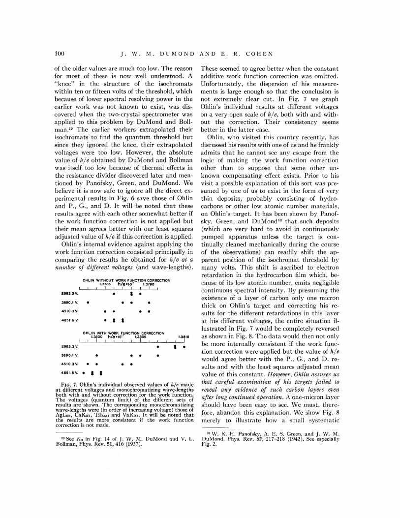
Fio. 7. Ohlin's individual observed values of ii/e madeat diAerent voltages and monochromatizing wave-lengthsboth with and without correction for the work function.The voltages (quantum limit) of the different sets ofresults are. showa, . The corresponding monochrornatizingwave-lengths were (in order of increasing voltage) those ofAgLai, CaKa~, TiKei and VaKn~. It will be noted thatthe results are more consistent if the work functioncorrection is not made.

"See Xs in Fig. 14 of J. W. M. DuMond and V. L.Bollman, Phys. Rev. $1, 416 (1937),

of the older values are much too low. I'he reasonfor most of these is now well understood. A"knee" in the structure of the isochromatswithin ten or fifteen volts of the threshold, whichbecause of lower spectral resolving power in theearlier work was not known to exist, was dis-covered when the two-crystal spectrometer wasapplied to this problem by DuMond and Boll-man. 's The earlier workers extrapolated theirisochromats to find the quantum threshold butsince they ignored the knee, their extrapolatedvoltages were too low. However, the absolutevalue of Ii/e obtained by DuMond and Bollmanwas itself too low because of thermal effects in

the resistance divider discovered later and men-tioned by Panofsky, Green, and DuMond. Webelieve it is now safe to ignore all the direct ex-perimental results in Fig. 6 save those of Ohlinand P, , G. , and D. It will be noted that theseresults agree with each other somewhat better ifthe work function correction is not applied buttheir mean agrees better with our least squaresadjusted value of Ji/e if this correction is applied.

Ohlin's internal evidence against applying thework function correction consisted principally in

comparing the results he obtained for Ji/e at anumber of dhgereut voltages (and wave-lengths)

These seemed to agree better when the constantadditive work function correction was omitted.Unfortunately, the dispersion of his measure-ments is large enough so that the conclusion isnot extremely clear cut. In Fig. 7 we graphOhlin's individual results at diR'erent voltageson a very open scale of Ji/e, both with and with-out the correction. Their consistency seemsbetter in the latter case.

Ohlin, who visited this country recently, hasdiscussed his results with one of us and he franklyadmits that he cannot see any escape from thelogic of making the work function correctionother than to suppose that some other un-known compensating effect exists. Prior to hisvisit a possible explanation of this sort was pre-sumed by one of us to exist in the form of verythin deposits, probably consisting of hydro-carbons or other low atomic number materials,on Ohlin's target. It has been shown by Panof-sky, Green, and DuMond" that such deposits(which are very hard to avoid in continuouslypumped apparatus unless the target is con-tinually cleaned mechanically during the courseof the observations) can readily shift the ap-parent position of the isochromat threshold bymany volts. This shift is ascribed to electronretardation in the hydrocarbon 61m which, be-cause of its low atomic number, emits negligiblecontinuous spectral intensity. By presuming theexistence of a layer of carbon only one micronthick on Ohlin's target and correcting his re-sults for the different retardations in this layerat his different voltages, the entire situation il-

lustrated in Fig. 7 would be completely reversedas shown in Fig. 8. The data would then not onlybe more internally consistent if the work func-tion correction were applied but the value of Ji/ewould agree better with the P., G. , and D. re-sults and with the least squares adjusted meanvalue of this constant. IIoveever, 0M' assures usthat careful examination of his targets failed to

reveal any evidence of such carbon layers even

after long continued operation. A one-micron layershould have been easy to see. We must, there-fore, abandon this explanation. We show Fig. 8merely to illustrate how a small systematic

~0 W. K. H. Panofsky, A. E. S. Green, and J. W. M.DuMond, Phys. Rev, 02, 217—218 (1942). See especiallyFig. 2,

ATOM I C CONSTANTS

source of error of this kind could aGect Ohlin's

conclusions regarding the invalidity of the workfunction correction. We are unable to see anyplausible reason for such a systematic errorhowever.

Ohlin has also tried comparing the values ofh/e he obtains using, on the one hand, an un-

coated tungsten cathode and, on the other hand,a BaO-coated platinum cathode. o' Here again theuncorrected value of h/e seemed to be inde-

pendent of the nature of the cathode. The workfunction of the coated cathode was presumablymuch lower than that of the tungsten. Unfor-

tuotately, il No case has Ohlil actually measured

the toork fulctiols of the cathodes he used Now. it is

a well-known fact that thermionic cathode workfunctions can vary widely (and either upward ordownward) from the influence of very slightcontaminations on their surfaces. In view of thetheoretical and practical importance of his re-sults we have urged him to repeat the experi-ments with provision for measuring his cathodework function. This can be done with sufhcientprecision for the purpose at hand by providingmeans of observing the cathode temperature andmeasuring the heating power which must besupplied to keep the cathode at constant tem-perature as a function of the emission currentdrawn off at diR'erent applied voltages.

On the theoretical side the absence of thenecessity for any cathode work. function correc-tion is very difFicult to understand. There canbe no doubt that the method of measuring theP.D. between the cathode and target of thetube with a resistance potential divider actuallymeasures the energy level difference (in volts)between the uppermost filled electron levels in

target and cathode terminals. Errors from ther-

1.3765I

2083.3'3690.1 V.

4510.3V.

4851.6 V.

ASSUMING ONK MICRON CARBON LAYERWITHOUT WORK FUNCTION CORRECTION .

ll.3770 h/e &10' 1.3775I I

~ ~

ASSUMING ONK MICRON CARBON LAYERWITH WORK FUNCTION CORRECTION

1,3785 h/e ~10 1.3790I I I I

2985.3V, )i ~ g ~

1.3795

3690.1 V.

45'I0. 3 V.

4651,e V.

P.G., D.

~ ~

DU MOND 8 COHKNLKAST SQUARES ADJ

mal e.m.f.'s, Kelvin P.D.'s, etc. are far too small

to be significant. Relative to the uppermost filled

levels in the target the electrons emitted fromthe cathode have received energy e V from thehigh potential source and energy ey from thethermal energy supplied to heat the cathodewhere V is the measured voltage and y thecathode work function. The maximum amountof energy available to convert into x-rays is

therefore e V+ey =ho,„,corresponding to transi-tions of cathode ray electrons to the lowest un-

filled final state in the target at the top of thepartially filled Fermi band. It would seem thatthis energy state for electrons would exist with-

Fm. 8. Ohlin's individual observed values of fo/e cor-rected for the existence of a hypothetical retarding layerof carbon deposit one micron thick on the target. Herethe results are more internally consistent if the workfunction correction is applied and also agree better withthe Io/e value of Panofsky, Green, and DuMond and withthe least squares adjusted value of fo/e from all sources.Ohlin is certain from inspection that no such depositsexisted on his target, and the plot is merely shown here toillustrate how small a systematic error of this sort couldreverse his conclusions regarding the inapplicability ofthe work function correction.

TABLE V. Values of constants on which computations are based (old viewpoint).

Inserted value

1 R = 109737.32 e 4.801933 e/m = 1.759034 fo/e = 1.378605 fo/(em)& = 1.000846 eo/(mto) =3.81977 m=7.30194X10 '8 Io/m = 7.267 (Gnan)8c io/m=7. 255 (R. and K.)

Origin value

R„p= 109737.08ep 4.80650eo/mo 1.75850too/eo = 1.38028fo /(e moo)& =o1.002157eoo/(mofoo) =3 81920np = 7.29870X 10too/mo = 7.27621too/mo = 7.27621

Relative difference

ag = 0.000002a& ——-0.000953as = 0.000302a4 = —0.00122as = —0.00132a6 = 0.000131a~ = 0.00044as = —0.00127

as, = —0.00292

Probable error

0.001.24X10 4

2.8 X10 4

2.9 X10 4

5.8 X10 4

10.5 X10-3.7 X 10-»

12.4 X10 4

30.3 X10 '

"P. Ohlin, Arkiv. f. Math. Astro. och Fysik 29B, No, 4.

TABI.E VI. Old viewpoint. Adjusted values of the atomicconstants and other derived constants. (Not recommendedbut given only for purposes of comparison. )

e= (4.8021+0.0005) )&10 '0 abs. e.s.u.m = (9.1055&0.0020) X 10—ss gh = (6.6233&0.0011))&10 '~ erg sec.F=9648.2+1.0 e.m.u. equiv. 'lV= (6.0229&0.0004) )& 10"mol '

e/m = (1.75927&0.00035) )&107 e.m.u. g 'h/e= {1.37924~0.00013))&10 '7 erg sec. e.s.u. '

a = (137.030+0.011) '),= (2.42645~0.00038) )&10 ' cm

out modification within a very few atom diam-eters of the target surface, and it is very difficultindeed to see any mechanism that can forbidtransitions of the impinging cathode rays tothis state. Such transitions will surely result in

the frequency r,„at the quantum limit of thecontinuous spectrum. It has been argued thatperhaps the transitions occur at the target surfaceor even just outside it and that the final state ofthe electron is therefore that of a free electronat the surface of the target. This electron byfurther transitions then eventually reaches thelevels of the conduction band inside the target.In such a case the equation of energy conversionwould become et/+eq, —etcs=hs, „and since

q, and y&, the work functions of cathode andtarget, respectively, are of the same order ofmagnitude, the net correction would be neg-ligible. The second subsequent transition to thetop of the Fermi sea would result in radiationtoo soft to be observed. Doubtless just suchmultiple transitions do occur but it still remainsunexplained why single transitions to the lowest

internal states are forbidden.There seems to be evidence in Ohlin's own iso-

chromats that the final state of the electron is

one of the permitted internal energy states orbands of the target lattice. The arguments lead-ing to this conclusion have been presented re-cently by DuMond. " If this is correct, it is verydificult to see how the lowest of these unfilledinternal states could be forbidden as a final statefor the impinging cathode ray-'electrons.

These diAiculties and uncertainties regardingthe work function correction, which in Ohlin's

work, because of his low voltages, would make alarge relative change in his numerical value ofh/e, have obliged us to omit using his results atthe present time. We have, therefore, based our

input value of h/e entirely on the P. , G. , and D.results corrected for the toorh function of the

tantalum cathode (4 volts or relatively only 2

parts in 10'). We have made a numerical testwhich shows that our final adjusted values ofthe constants are insignificantly aff'ected by achange of the order of this work function in ourcase. We have increased the estimated probableerror of the P., G. , and D. results from ~0.0002to ~0.0004 because of the uncertainty regardingthe value of the work function which, as we havepointed out above, might have been considerablyincreased or decreased by surface contamina-tions. We thus arrive at the following inputvalue:

h/e =hN/F = (1.3786&0.0004))&10 "erg sec. e.s.u

M. h/(em)'* from Von Friesen's ElectronDi6'rat:tion Exyeriments

For this constant we have used, withoutmodification, the value recomputed earlier by

TABLE VII. Input values, new viewpoint.

1. N= (6.02338+0.00043) X 10" (chemical scale)2. F=9648.5 +1.0 abs. e.m. u. equiv. ' (chemical scale)3. mN= (R /2ar cs)F Nsk = (5.48541+0.00075) X10 4 (chemical scale)4. F(e/m) = (2ar'c'/R )F'N sk '=(1.69824&0.00035) XIOu (chemical scale)5. e/m= (2arac /R )FsN sk = (1 75920&0 0. 0038) X I.Oa e.m.u. g6. k/e=ckN/F=1. 3786&0.0004 erg sec. e.s.u. '7. =as2arcFaN'k '= (136.95&0.05) '8. k/(em)&=( 2araca/R)&k &F&N &=(1.00084+000058)X10 s e.s.u.9. k/m= (2araca/R )FsN 4k '=7.267+0009 cg.s. unit

10. e'/mk=(2aracs/R )F'N 'k "=(3.8197&00045)X10s4 e su.

Source

X-ray crystal methodI and Ag voltametersSpectroscopic fine structureX-ray refractive index of diamondDeflection methods; Zeeman effectContinuous x-ray spectrumX-ray doublets (Christy and I&eller)Von Friesen experimentGnan experimentRobinson and co-workers

'- J. W. M. DuMond, Phys. Rev. 72, 276 {1947).

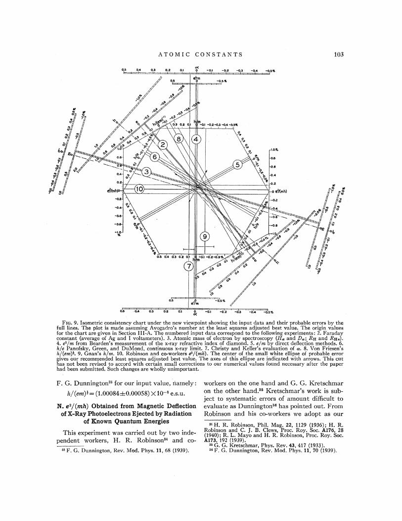
ATOM I C CONSTANTS 103

0.5 0.4 0.3 0.2cK

O.l 0 -O.I -0.2I

-0.3 -04f 0)%

-0.5%

I ii'mOl ~.2M.3~M5%

a», I I I I l~

-l.0Fo

LP+

2

0.5 0.4 0.3 0.2 O. ll&~

0.5

0.5 0& 0.3 0.2 0.$

pe/m

b O.l 0.2 0.3 W.4 0 5fo0(

FIG. 9. Isometric consistency chart under the new viewpoint showing the input data and their probable errors by thefull lines. The plot is made assuming Avogadro's number at the least squares adjusted best value. The origin valuesfor the chart are given in Section III-A. The numbered input data correspond to the following experiments: 2. Faradayconstant (average of Ag and I voltameters). 3. Atomic mass of electron by spectroscopy (H and D; Rn and RH,).4. ez/zzz from Bearden's measurement of the x-ray refractive index of diamofzd. 5. e/zzz by direct deflection methods. 6.lz/e Panofsky, Green, and DuMond, continuous x-ray limit. I. Christy and Keller's evaluation of u. 8. Von Friesen'sfz/(ezzz)&. 9. Gnan's fz/zzz. 10. Robinson and co-workers sz/(zzzfz). The center of the small white ellipse of probable errorgives our recommended least squares adjusted best value. The axes of this ellipse are indicated with arrows. This cuthas not been revised to accord with certain sma11 corrections to our numerical values found necessary after the paperhad been submitted. Such changes are wholly unimportant.

F. G. Dunnington" for our input value, namely:

b/(ezzz) & = (1.00084+0.00058) X 10—' e.s.u.

N. e'/(mjt) Obtained from Magnetic Deflectionof X-Ray Photoelectx'ons Ejected. by Radiation

of Known Quantum Energies

This experiment was carried out by two inde-pendent workers, H. R. Robinson'4 and co-

"F.G. Dunnington, Rev. Mod. Phys. 11, 68 (1939).

workers on the one hand and G. G. Kretschmaron the other hand. "Kretschmar's work is sub-ject to systematic errors of amount dif6cult toevaluate as Dunnington' has pointed out. FromR.obinson and his co-workers we adopt as our

z' H. R. Robinson, Phil. Mag. 22, 1129 (1936); H. R.Robinson and C. J. B. Clews, Proc. Roy. Soc. A176, 28(1940); R. L. Mayo and H. R. Robinson, Proc. Roy. Soc.A1V3, 192 (1939).

» G. G. Kretschmar, Phys. Rev. 43, 417 (1933).zz F. G. Dunnington, Rev. Mod. Phys. 11, VO (1939).

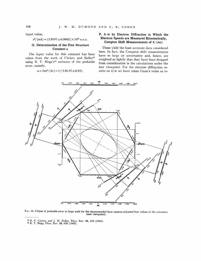
J. '|A". M. D UMON D AND E. R. COHEN

input value,

e'/(mh) = (3.8197~0.0045) &(10s4 e.s.u.

O. Determination of the Fine StructureConstant e

The input value for this constant has beentaken from the work of Christy and Keller'rusing R. T. Birge's38 estimate of the probableerror, namely,

o. =2se'/(hc) = 1/(136.95&0.05).

P. A/m by Electron Diffraction in Which theElectron Speeds are Measured Kinematically,

Compton Shift Measurements of A/(mc)

These yield the least accurate data consideredhere. In fact, the Compton shift measurementshave so large an uncertainty and, hence, areweighted so lightly that they have been droppedfrom consideration in the calculations under thenew viewpoint. For the electron diffraction re-sults on k/nz we have taken Gnan's value as re-

0.008 0.008 0.004 0.002 0 0.002 -0.004 0.008 -0.008 0.01 +I

0,'0~ O.OO8 O.OO8'

0.004 O.002 b -O.OO2 -O.OO4'

-O.OO8 -00O8 -O'e%tX

F&G. &0. El&ipse of probable error to large scale for the recommended least squares adjusted best values of the constants(new viewpoint).

~r R. F. Christy and J. M. Keller, Phys. Rev. 58, 658 (1940).» R. T. Birge, Phys. Rev. 58, 658 (1940).

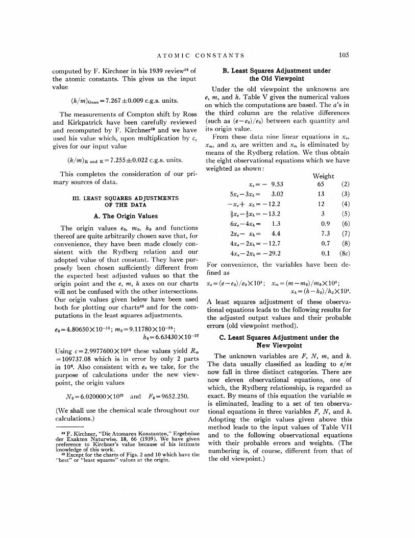
ATOMIC CONSTANTS

computed by F. Kirchner in his 1939 review 9 ofthe atomic constants, This gives us the inputvalue

(7i/m)G„, „=7.267&0.009 c.g.s. units.

The measurements of Compton shift by Rossand Kirkpatrick have been carefully reviewedand recomputed by F. Kirchner'9 and we haveused his value which, upon multiplication by c,gives for our input value

(h/m)R, „d K ——7.255 &0.022 c.g.s. units.

This completes the consideration of our pri-mary sources of data.

III. LEAST SQUARES ADJUSTMENTSOF THE DATA

A. The Origin Values

The origin values eo, mo, ho and functionsthereof are quite arbitrarily chosen save that, forconvenience, they have been made closely con-sistent with the Rydberg relation and ouradopted value of that constant. They have pur-

posely been chosen sufficiently different fromthe expected best adjusted values so that theorigin point and the e, m, h axes on our chartswill not be confused with the other intersections.Our origin values given below have been usedboth for plotting our charts" and for the com-putations in the least squares adjustments.

co=4.80650X10 ";m0=9. 11780X10—";h0=6.63430X10 '~

Using c=2.9977600X10" these values yield R=109737.08 which is in error by only 2 partsin 10'. Also consistent with eo we take, for thepurpose of calculations under the new view-

point, the origin values

Xo = 6.020000 X 10" and Ji 0 =9652.250.

(We shall use the chemical scale throughout ourcalculations. )

"F.Kirchner, "Die Atomaren Konstanten, " Ergebnisseder Exakten Naturwiss. 18, 66 (1939). Ke have givenpreference to Kirchner's value because of his intimateknowledge of this work.' Except for the charts of Figs. 2 and 10 which have the"best" or "least squares" values at the origin.

3. Least Squares Adjustment underthe Old Viewpoint

Vnder the old viewpoint the unknowns aree, m, and h. Table V gives the numerical valueson which the computations are based. The a's in

the third column are the relative differences(such as (e —eo)/eo) between each quantity andits origin value.

From these data nine linear equations in x, ,

x. , and x~, are written and x, is eliminated bymeans of the Rydberg relation. We thus obtainthe eight observational equations which we haveweighted as shown:

x, = —9.53

3.02—x,+ x(,

6x,—4xp,

2xs xII,

4x, —2xg

4x.—2xJ,

1202

1302

1.3

1207

—29.2

Weight65 (2)

(3)

(4)

(5)0.9 (6)7.3 (7)0.7 (8)0.1 (8c)

For convenience, the variables have been de-fined as

x, = (e —eo)/eo X 10'; x = (m —mo)/ma X 10';xI„= (&—&0)/&~ X 10'.

A least squares adjustment of these observa-tional equations leads to the following results forthe adjusted output values and their probableerrors (old viewpoint method).

C. Least Squares Adjustment under theNew Viewpoint

The unknown variables are F, N, m, and h.The data usually classified as leading to e/mnow fall in three distinct categories. There arenow eleven observational equations, one ofwhich, the Rydberg relationship, is regarded asexact. By means of this equation the variable m

is eliminated, leading to a set of ten observa-tional equations in three variables Ii, X, and h.Adopting the origin values given above thismethod leads to the input values of Table VIIand to the following observational equationswith their probable errors and weights. (Thenumbering is, of course, diR'erent from that ofthe old viewpoint. )

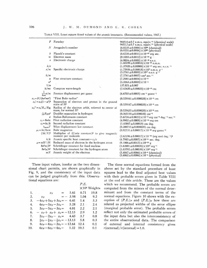
YV. A1. 0 U MON B AND E, R. COHEN

TAm, E VIII. Least square fitted values of the atomic'constants. I'Recommended values, i947.)

P Faraday

à Avogadro's number

Planck" s constantm Electron masse Flectronic charge

A/e

e/ns Specific electronic charge

h/m

cF

1/ak/mc

j.—e/ns4mc

a, =k'/(4s'me')ao'= ao(1 —a')'

ao"——ao'R„/RH

—'RHa'

cg ——8~bces = ke/k

~max &

p, g——he/4~m

(3k/X)1

h/kp= mH+/H

8s'm/k'8ssy/k2

mX

Fine structure constant

Compton wave-length

Zeeman displacement per gauss

"First Bohr radius"Separation of electron and proton in the groundstate of H'Radius of the electron orbit, referred to center ofmass, for normal H'Doublet separation in hydrogenStefan-Boltzmann constantFirst radiation constantSecond radiation constantMien displacement law constantBohr magnetonMultiplier of (Curie constant)& to give magneticmoment per moleculeAtomic specific heat constant=eq/cReduced mass of electron in the hydrogen atomSchrodinger constant for fixed nucleusSchrodinger constant for the hydrogen atomAtomic weight of the electron

9649.6&0.7 e.m. u. equiv. ' (chemical scale)9652.2 &0.7 e.m. u. equiv. ' (physical scale)(6.0235 &0.0004) X 10~~ (chemical)(6.0251+0.0004) X10" (physical)(6.6234~0.0011)X 10~' erg sec.(9 1055+0.0012)X10~' g—(& 8024+0.0005) X &0 ."e.s.u.(1.60199&0.00016)X 10 "e.m. u.(1.37920+0.00009) X 10 "erg sec. e.s.n. "

(1.75936g0.00018)X 10' e.m. u. 8 &

(5.2741&0.0005) X10"e. .u. g '(7.2741&0.0007) cm' sec. '

(7 2981+0.0004) X 10 '(5 3263+0.0005) X10 '137.021&0.007(2 42650~0 00025) X 10—10 cm

(4.6703+0.0005) cm ' gauss '

(0.529161+0.000028) X 10 ' cm

(0 529147+0.000028) X 10 ' cm

(0.529435+0.000028) X10 ' cm(0.365110&0.000038) cm '(5.6724+0.0023) X10 s erg cm ' deg. ' sec. '(4.9902&0.0008) X 10 '~ erg cm(1.43847*0.00019) cm deg.(0.289715&0.000039) cm deg.(0.92731+0.00017)X10 "erg gauss '

(2.62196+0.00017)X 10 " (erg mol deg. ')&

(4.7985&0.0007) X10 "sec. deg.(9 1006+0 0012)X 10 ~s g(1.63881+0.00039)X10'~ erg '(1 63792+0.00039)X 10sr erg ~

(5.4847&0.0006) X10 4 (chemical)(5.4862 +0.0006) X 10 ' (physical)

2.3.

5..6.7.8.9.

10.

xp'—4xg+Sx~+3xp, =

6xp —Sx~ —3',=5xp —5xy —3XI,=Xp+ X++ Xs

2xp 2xpf xA, —PXP' 2X2v g Xg—3 3

4x p—4X~ —2XI, =

6xp —6x~ —4xg, =

5.61—3.98

6.415.284.01

—12.154.43

—13.13—12.64

1.32

I'.E.X10'0.711.041.42.1

2.22.93.75.8

12,410.5

Weights

19.89.25.32.42.1

1.20.80.30.1

0.1

These input values, insofar as the two dimen-sional chart permits, are shown graphically in

Fig. 9, and the consistency of the input datacan be judged. graphically from this. Observa-tional equations are:

The three normal equations formed from theabove set by the standard procedure of leastsquares lead to the final adjusted best valueswith their probable errors given in Table VIIIat the end of this article. These are the valueswhich we recommend. The probable errors arecomputed from the minors of the normal deter-minant and from the constant terms of thenormal equations. Figure 10 shows with the ex-ception of (I'.B.)~ and (P.B.)~ how these arerelated as projected widths of the error ellipse(marginal probable error). The probab1e errorsreHect not only the estimated probable errors ofthe input data but also the interconsistency ofthe entire observational data. The comparisonof external and interrial consistency givesr(external)/r(internal) = 1.0.

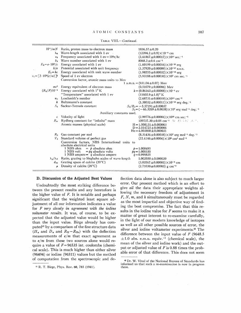
ATO M I C CONSTAN TS

I ABLE VI II.—Continued.H+/@zan

Xo

&0

(Ro/F) 10—8

no

So

1836.57~0.20(12394.2+0.9) X 10 ' cm(2.4186/&0.00017)X 10'4 sec.8068.2&0.6 cm '(1.60199+0.00016)X 10 "erg.

(1 37920+0.00009)X 10 "e.s.u.(1 98555&0.00032)X10 "erg(5.93188&0.00030) X 10' cm sec. '

Ratio, proton mass to electron massWave-length associated with 1 evFrequency associated with 1 ev= 10'e/bcWave number associated with 1 evEnergy associated with 1 evPotential associated with unit frequencyEnergy associated with unit wave numberSpeed of 1 ev electronConversion factor, atomic mass units to Mev

1 a..m. u. = (931.04&0.07) MevEnergy equivalent of electron mass (0.51079&0.00006) MevEnergy associated with 1 K k = (0.86163~0.00008) X 10 4 ev"Temperature" associated with 1 ev (11605.9&1.0)' KLoschmidt's number (2 68731&0.00019)X 10"cm 'Boltzmann's constant (1.38032&0.00011)X10 '6 erg deg. ~

Sackur-Tetrode constant Sp/Rp ———5.57191&0.0003750=(—46.3269+0.0038)X10 erg mol ' deg. '

Auxiliary constants used.(2.99776&0.00004) X10"cm sec. '109737.30&0.05 cm ' --- /."". '-. -& '"

H = 1.008131~0.000003D =2.0 1.4725 ~0.000006

He =4.00386040.000031(8.31436&0.00038) X 10r erg mol ' deg. '(22.4146&0.0006) X 10' cm' mol '

c Velocity of lightRydberg constant for "infinite" massAtomic masses (physical scale)

~0Vp

P = 1.000495Pg = 1.000330

g =0.9998351.002030+0.000020(3.03'S67&0.00005) X 10 ' cm(2.71030&0.00003) g cm '

l g/Xsd2o

P

Gas constant per molStandard volume of perfect gasConversion factors, NBS International uni, ts toabsolute electrical units

1 NBS ohm = p absolute ohm1 NBS volt =pq absolute volts1 NBS ampere= q absolute ampere

Ratio, grating to Siegbahn scales of wave-lengthGrating space of calcite (20'C)Density of calcite (20'C)

D. Discussion of the Adjusted Best Values

Undoubtedly the most striking difference be-tween the present results and any heretofore isthe higher value of Ii. It is notable and perhapssignificant that the weighted least square ad-justment of all our information indicates a valuefor Ji very closely in agreement with the iodinevoltameter results. It was, of course, to be ex-pected that the adjusted value would be higherthan the input value. Birge already has com-puted" by a comparison of the fine structure data(II and D and Rn —RH, ) with the deflectionmeasurements of e/m that exact agreement asto e/m from these two sources alone would re-quire a value of F=96535 int. coulombs (chemi-cal scale). This is much higher than either silver(96494) or iodine (96511) values but the methodof computation from the spectroscopic and de-

"R. T. Birge, Phys. Rev. 60, 785 (1941),

Hection data alone is also subject to much largererror. Our present method which is an effort togive all the data their appropriate weights al-lowing the necessary freedom of adjustment inF, N, m, and h simultaneously must be regardedas the most impartial and objective way of find-ing the best compromise. The fact that this re-sults in the iodine value for F seems to make it amatter of great interest to re-examine carefully,in the light of our modern knowledge of isotopesas well as all other possible sources of error, thesilver and iodine voltameter experiments. "Thedifference between the input value of Ii (9648.5+1.0 abs. e.m. u. equiv. ' (chemical scale), themean of the silver and iodine work) and the out-put or adjusted value of Ii is 0.88 times the prob-able error of that difference. This does not seem

~ Dr. W. Vinal of the National Bureau of Standards hasinformed us that such a re-examination is now in progressthere.

108 J. K. M. D U MON D AN D E. R. COH EN

serious and we feel no hesitancy in recommend-ing our value for adoption since it results inbetter agreement with all our sources of informa-tion than any other.

It will be noted that the adjusted value of Nhas changed very little indeed from our inputvalue or from the values recommended in thepast. This should be a source of considerablesatisfaction to the workers (Bearden, Backlin,Sodermann) who have devoted such care to thisimportant constant with such eminently satis-factory results. There is a slight upward shift ine which is chieHy ascribable to the upward shiftin Ii but the change is well inside the probableerror of the diFference between input or outputvalues. The adjusted output value of h/e ex-ceeds the Panofsky, Green, and DuMond (in-

put) value by 1.5 times the probable error ofthis diFference. This cannot be taken as proof ofsystematic errors in the measurement since sucha deviation is not considered as excessive. Theresults of Ohlin's investigations as regards thework function correction should prove of greatvalue. Should it develop that the work functionmust be added as a correction to his present re-suIts, then the average of Ohlin and P., G. , andD. as to h)e will be in substantially better agree-ment with our present adjusted best value thanP., G. , and D. alone is now. If the work functioncorrection is not made, however, the discrepancyfrom our best adjusted value will be serious.

In a very recent redetermination4' at the Na-

3M. S. Van Dusen and A. I. Dahl, N.B.S. Researchpaper, RP 1828 from Bur. Stand. J. Research 39, 291(1947).

tional Bureau of Standards of the second radia-tion constant c2 by direct experimental meansthe mean result, c2 ——1.4382 cm degrees has beenobtained. (The three different individual resultsfrom which this mean is derived indicate by theirconsistency a probable error of ~0.0006 in thea,bove figure. ) This agrees very well with (1) R.T. Birge's indirectly calculated 1941 value,cs ——1.43848&0.00034 and (2) our present recom-mended value from our least squares adjustment,c2=1.43847~0.00019. As Dr. Birge has pointedout in a recent letter to us, the InternationalTemperature Scale has been and still is based onthe value c2 = 1.432, the same value as that recom-mended by him in 1929. Until the present work4'

there never had been an experimental valuehigher than c2 ——1.436 and this was one of thegreat discrepancies between directly observedand calculated values. This situation is, therefore,very much more satisfactory than ever before.

The chart, Fig. 9, shows that none of the inputvalues of our data represented thereon deviatefrom our best adjusted output values seriouslywhen each deviation is compared with the prob-able error spread of that input datum.

ACKNOWLEDGMENTS

The authors are much indebted to ProfessorR. T. Birge for pointing out the oversight, in

their original manuscript, of his improved resultsregarding Avogadro's number which are pub-lished in his 1945 paper. ' The numerical valuesin the present paper have been revised to accordwith this result.