orthogonal statistical learning - arxivorthogonal statistical learning dylan j. foster mit...
TRANSCRIPT

Orthogonal Statistical Learning
Dylan J. FosterMIT
Vasilis SyrgkanisMicrosoft Research, New England
Abstract
We provide excess risk guarantees for statistical learning in a setting where the populationrisk with respect to which we evaluate the target model depends on an unknown model thatmust be to be estimated from data (a “nuisance model”). We analyze a two-stage samplesplitting meta-algorithm that takes as input two arbitrary estimation algorithms: one for thetarget model and one for the nuisance model. We show that if the population risk satisfies acondition called Neyman orthogonality, the impact of the nuisance estimation error on the excessrisk bound achieved by the meta-algorithm is of second order. Our theorem is agnostic to theparticular algorithms used for the target and nuisance and only makes an assumption on theirindividual performance. This enables the use of a plethora of existing results from statisticallearning and machine learning literature to give new guarantees for learning with a nuisancecomponent. Moreover, by focusing on excess risk rather than parameter estimation, we can giveguarantees under weaker assumptions than in previous works and accommodate the case wherethe target parameter belongs to a complex nonparametric class. We characterize conditions onthe metric entropy such that oracle rates—rates of the same order as if we knew the nuisancemodel—are achieved. We also analyze the rates achieved by specific estimation algorithmssuch as variance-penalized empirical risk minimization, neural network estimation and sparsehigh-dimensional linear model estimation. We highlight the applicability of our results in foursettings of central importance in the literature: 1) heterogeneous treatment effect estimation, 2)offline policy optimization, 3) domain adaptation, and 4) learning with missing data.
Contents
1 Introduction 3
2 Framework: Statistical Learning with a Nuisance Component 6
3 Orthogonal Statistical Learning 83.1 Fast Rates Under Strong Convexity . . . . . . . . . . . . . . . . . . . . . . . . . . . . . . 93.2 Beyond Strong Convexity: Slow Rates . . . . . . . . . . . . . . . . . . . . . . . . . . . . 11
4 Sufficient Conditions for Single Index Losses 114.1 Fast Rates . . . . . . . . . . . . . . . . . . . . . . . . . . . . . . . . . . . . . . . . . . . . . 114.2 Slow Rates . . . . . . . . . . . . . . . . . . . . . . . . . . . . . . . . . . . . . . . . . . . . . 13
5 Empirical Risk Minimization with a Nuisance Component 145.1 Fast Rates via Local Rademacher Complexities . . . . . . . . . . . . . . . . . . . . . . . 15
5.1.1 Fast Rates for Specific Classes . . . . . . . . . . . . . . . . . . . . . . . . . . . . 165.2 Slow Rates and Variance Penalization . . . . . . . . . . . . . . . . . . . . . . . . . . . . 19
5.2.1 Application to VC Classes . . . . . . . . . . . . . . . . . . . . . . . . . . . . . . . 21
1
arX
iv:1
901.
0903
6v2
[m
ath.
ST]
11
Mar
201
9

6 Minimax Oracle Rates for Square Losses 236.1 Rates for First Stage . . . . . . . . . . . . . . . . . . . . . . . . . . . . . . . . . . . . . . . 246.2 Minimax Oracle Rates . . . . . . . . . . . . . . . . . . . . . . . . . . . . . . . . . . . . . . 266.3 Sketch of Proof Techniques . . . . . . . . . . . . . . . . . . . . . . . . . . . . . . . . . . . 27
7 Minimax Oracle Rates for Generic Lipschitz Losses 29
8 Applications 308.1 Treatment Effect Estimation . . . . . . . . . . . . . . . . . . . . . . . . . . . . . . . . . . 308.2 Policy Learning . . . . . . . . . . . . . . . . . . . . . . . . . . . . . . . . . . . . . . . . . . 338.3 Domain Adaptation and Sample Bias Correction . . . . . . . . . . . . . . . . . . . . . . 368.4 Missing Data . . . . . . . . . . . . . . . . . . . . . . . . . . . . . . . . . . . . . . . . . . . 38
9 Discussion 39
A Preliminaries 44
B Proofs from Section 3 44
C Proofs from Section 4 46
D Preliminary Theorems for Constrained M-Estimators 49D.1 Proofs of Lemmas for Constrained M -Estimators . . . . . . . . . . . . . . . . . . . . . 51
E Proofs from Section 5 53E.1 Proof of Theorem 3 . . . . . . . . . . . . . . . . . . . . . . . . . . . . . . . . . . . . . . . 54E.2 Proofs for Specific Function Class Guarantees . . . . . . . . . . . . . . . . . . . . . . . 59E.3 Proof of Theorem 4 . . . . . . . . . . . . . . . . . . . . . . . . . . . . . . . . . . . . . . . 62E.4 Proof of Theorem 5 . . . . . . . . . . . . . . . . . . . . . . . . . . . . . . . . . . . . . . . 63E.5 Proof of Theorem 6 . . . . . . . . . . . . . . . . . . . . . . . . . . . . . . . . . . . . . . . 63
F Proofs from Section 6 and 7 68F.1 Preliminaries . . . . . . . . . . . . . . . . . . . . . . . . . . . . . . . . . . . . . . . . . . . 68F.2 Skeleton Aggregation . . . . . . . . . . . . . . . . . . . . . . . . . . . . . . . . . . . . . . 70F.3 Rates for Specific Algorithms . . . . . . . . . . . . . . . . . . . . . . . . . . . . . . . . . 70F.4 Proofs for Oracle Rates . . . . . . . . . . . . . . . . . . . . . . . . . . . . . . . . . . . . . 74
G Proofs from Section 8 76
2

1 Introduction
Predictive models based on modern machine learning methods are becoming increasingly widespreadin policy making, with applications in health care, education, law enforcement, and business decisionmaking. Most problems that arise in policy making, such as attempting to predict counterfactualoutcomes for different interventions or optimizing policies over such interventions, are not pureprediction problems, but rather are causal in nature. It is important to address the causal aspect ofthese problems and build models that have a causal interpretation.
A common paradigm in the search of causality is that to estimate a model with a causalinterpretation from observational data—for example, data not collected via randomized trial orvia a known treatment policy—one typically needs to estimate many other quantities that are notof primary interest, but that can be used to de-bias a purely predictive machine learning modelby formulating an appropriate loss. Examples of such nuisance parameters include the propensityfor taking an action under the current policy, which can be used to form unbiased estimates forthe reward of new policies, but is typically unknown in datasets that do not come from controlledexperiments.
To make matters more concrete, let us walk through an example for which certain variants havebeen well-studied in machine learning (e.g., Dudık et al. (2011); Swaminathan and Joachims (2015a);Nie and Wager (2017); Kallus and Zhou (2018)). Suppose a decision maker wants to estimate thecausal effect of some treatment T ∈ 0,1 on an outcome Y as a function of a set of observablefeatures X; the causal effect will be denoted as θ(X). Typically, one has access to data consistingof tuples (Xi, Ti, Yi), where Xi is the observed feature for sample i, Ti is the treatment taken, andYi is the observed outcome. Such settings are often referred to as having bandit feedback, sincewe only observe the outcome for the treatment that was chosen. Due to the bandit nature of theproblem, one needs to create unbiased estimates of the unobserved outcome. A standard approachis to use the so-called doubly-robust formula, which is a combination of direct regression and inverse
propensity scoring: if we let Y(t)i denote the potential outcome from treatment t in sample i, and let
m(t)0 (xi) ∶= E[Y
(t)i ∣ xi] and p
(t)0 ∶= E[1T = t∣xi], then the following is an unbiased estimator for
each potential outcome:
Y(t)i =m
(t)0 (xi) +
(Yi−m(t)0 (xi))1Ti=t
p(t)0 (xi)
(1)
Given such an estimator, we can estimate the treatment effect by running a regression between the
unbiased estimates and the features, i.e. solve minθ∈Θn∑i (Y(1) − Y (0) − θ(Xi))
2over some model
class Θn. In the population limit, with infinite samples, this corresponds to finding a model θ(x)
that minimizes the population risk E[(Y(1)i − Y
(0)i − θ(X))2]. Similarly, if one is interested in policy
optimization rather than estimating treatment effects, they could use these unbiased estimates
to solve minθ∈Θn∑i(Y(0)i − Y
(1)i ) ⋅ θ(Xi) over a policy space Θn of functions mapping features to
0, 1. When dealing with observational data, the functions m0 and p0 are not known, and must beestimated if we wish to evaluate the proxy labels Y (t).The goal of the learner is to find a model θthat achieves good population risk when evaluated at the true nuisance functions as opposed to theestimated, since only then the model has a causal interpretation.
This phenomenon is ubiquitous in causal inference and motivates us to formulate the abstractproblem of statistical learning with a nuisance component: Given n i.i.d. examples from a distributionD, a learner is interested in finding a target model θn ∈ Θn so as to minimize a population riskfunction LD ∶ Θn ×Gn → R. The population risk depends not just on the target model, but also on anuisance model whose true value g0 ∈ Gn is unknown to the learner. The goal of the learner is to
3

produce an estimate that has small excess risk evaluated at the unknown true nuisance model:
LD(θn, g0) − infθ∈Θn LD(θ, g0). (2)
Depending on the application such an excess risk bound can take different interpretations. Formany settings, such as treatment effect estimation, it is closely related to mean squared error, whilein policy optimization problems it may correspond to regret. Following the tradition of statisticallearning theory (Vapnik, 1995; Bousquet et al., 2004), we make excess risk the primary focus of ourwork, independent of the interpretation. We develop algorithms and analysis tools that genericallyaddress (2), then apply these tools to a number of applications of interest.
The problem of statistical learning with a nuisance component is strongly connected to theproblem of semiparametric inference (Robinson, 1988; Kosorok, 2008), where a true parameterθ0 is the minimizer of a population risk that depends on unknown nuisance components. Ourpaper builds on a growing body of results on “double” or “debiased” machine learning in statisticsand econometrics literature (Chernozhukov et al., 2017, 2018a,c,b) for addressing semiparametricinference problems. This line of research has focused on providing so-called “
√n-consistent and
asymptotically normal” estimates when the target parameter θ0 is low-dimensional and nuisanceparameters belong to a nonparametric class. Unlike the semiparametric inference problem, statisticallearning with a nuisance component does not require a well-specified model, nor a unique minimizerof the population risk. Moreover, we do not ask for parameter recovery and asymptotic inference(i.e. asymptotically valid confidence intervals). Rather, we are content with an excess risk bound,regardless of whether there is an underlying true parameter to be identified. As a consequence, weprovide guarantees even when the target model belongs to a large, potentially nonparametric class.
The case where the target parameter belongs to an arbitrary class has not been addressed atthe level of generality we consider in the present work, but we mention some prior work that goesbeyond the low-dimensional/parametric setup for special cases. Athey and Wager (2017) and Zhouet al. (2018) give guarantees based on metric entropy of the target class for the specific problemof treatment policy learning. For estimation of treatment effects, various nonparametric classeshave been used for the target class on a fairly cases by case basis, including kernels (Nie andWager, 2017), random forests (Athey et al., 2016; Oprescu et al., 2018; Friedberg et al., 2018), andhigh-dimensional linear models (Chernozhukov et al., 2017, 2018b). Our work unifies several ofthese papers into a single framework and our general results have implications and improve uponeach of these directions (see Section 8 for a detailed comparison).
Our approach is to reduce the problem of statistical learning with a nuisance component to thestandard formulation of statistical learning. Rather than directly analyzing particular algorithmsand models from machine learning (e.g., regularized regression, gradient boosting, or neural networkestimation) we assume a black-box guarantee for the excess risk in the case where a nuisance valueg ∈ Gn is fixed. Our main theorem asks only for the existence of an algorithm Alg(Θn, S ; g) that, forany given nuisance model g and data set S, achieves good excess risk with respect to the populationrisk LD(θ, g), i.e. with probability 1 − δ:
LD(θn, g) − infθ∈Θn
LD(θ, g) ≤ RateD(Θn, S, δ ; g). (3)
Likewise, we assume the existence of a black-box algorithm Alg(Gn, S) to estimate the nuisancecomponent g0 from the data, with the required estimation guarantee varying from problem toproblem.1
1Our approach is conceptually related to Kunzel et al. (2017), who studied meta-algorithms based on off-the-shelflearning procedures for the specific problem of estimating the conditional average treatment effect, albeit our resultsare technically very different.
4

Meta-Algorithm 1 (Two-Stage Estimation with Sample Splitting).Input: Sample set S = z1, . . . , zn.
• Split S into subsets S(1) = z1, . . . , z⌊n/2⌋ and S(2) = S ∖ S(1).
• Let gn be the output of Alg(Gn, S(1)).
• Return θn, the output of Alg(Θn, S(2) ; gn).
Given access to the two black-box algorithms, we analyze a simple sample splitting-basedmeta-algorithm for statistical learning with a nuisance component, presented as Meta-Algorithm 1.We can now state the main question addressed in this paper: When is the excess risk achieved bysample splitting robust to nuisance component estimation error?
In more technical terms, we seek to understand when the two-stage sample splitting estimationalgorithm achieves an excess risk bound with respect to g0, in spite of error in the estimator gnoutput by the first-stage algorithm. Robustness to nuisance estimation error allows the learner touse more complex models for nuisance estimation and—under certain conditions on the complexityof the target and nuisance model classes—to learn target models whose error is, up to lower orderterms, as good as if the learner had known the true nuisance model. Such a guarantee is typicallyreferred to as achieving an oracle rate in semiparametric inference.
Overview of results. We show that Neyman orthogonality, which has been used to prove oraclerates for inference in semiparametric models (Neyman, 1959, 1979; Chernozhukov et al., 2018a,b), iskey to providing oracle rates for statistical learning with a nuisance component. We prove that if thepopulation risk satisfies a functional analogue of Neyman orthogonality, then the estimation errorof gn has a second order impact on the overall excess risk (relative to g0) achieved by θn. To gainsome intuition, Neyman orthogonality is weaker condition than double robustness, albeit similar inflavor, (see e.g. Chernozhukov et al. (2016)) and is satisfied by both the treatment effect loss andthe policy learning loss described in the introduction. In more detail, our extension of the Neymanorthogonality condition asks that a cross-functional derivative of the loss vanish to zero, whenevaluated at the optimal target and nuisance models. Prior work on the classical notion of Neymanorthogonality provides a number of means through which to construct orthogonal losses whenevercertain moment conditions are satisfied by the data generating process (Chernozhukov et al., 2018a,2016, 2018b). Indeed, orthogonal losses can be constructed in settings including treatment effectestimation, policy learning, missing data problems, estimation of structural econometric problemsand game theoretic models.We identify two regimes of excess risk behavior:
1. When the population risk is strongly convex with respect to the prediction of the target model(e.g. the treatment effect estimation loss), then typically so-called fast rates (e.g. rates of orderof O(1/n) for parametric classes) are achievable had we known the true nuisance model. LettingRGn denote the estimation error of the nuisance component (root-mean-squared predictionerror for most of our settings), then in the fast rate setting we show that orthogonality impliesthat the first stage error has an impact on the excess risk of the order of R4
Gn(e.g. n−1/4
RMSE rates for the nuisance suffice when the target is parametric).
2. Absent any assumption on the convexity of the population risk (e.g. the treatment policyoptimization loss), then typically slow rates (e.g. rates of order O(1/
√n) for parametric
classes) are achievable had we known the true nuisance model. In this case the impact is
5

of nuisance estimation error is of the order R2Gn
so, once again, n−1/4 RMSE rates for thenuisance suffice when the target is parametric.
To extend the sufficient conditions above to arbitrary classes, we give conditions on the relativecomplexity of the target and nuisance classes—quantified via metric entropy—under which thesample splitting meta-algorithm achieves oracle rates (assuming the two black-box estimationalgorithms are appropriately instantiated). This allows us to extend several prior works beyond theparametric regime to complex nonparametric target classes. Our technical results extends the worksof Yang and Barron (1999); Rakhlin et al. (2017), which provide minimax optimal rates withoutnuisance components and utilize the technique of aggregation in designing optimal algorithms.
The flexibility of our approach allows us to instantiate the framework with any machine learningmodel and algorithm of interest for both nuisance and target model estimation, and to utilizethe vast literature on generalization bounds in machine learning to establish data-dependent anddimension-independent rates for several classes of interests. For instance, our approach allows usto use recent work on size-independent generalization error of neural networks. We obtain sharpguarantees for these specific model classes and more as a consequence of a new analysis for empiricalrisk minimization with plug-in estimation of nuisance parameters in the presence of orthogonality.Our results on plugin empirical risk minimization extend the local Rademacher complexity analysisof generalization bounds (Koltchinskii and Panchenko, 2000; Bartlett et al., 2005), to account for theimpact of the nuisance error. In the slow rate regime we also give a new analysis of variance-penalizedempirical risk minimization, which allows us to recover and extend several prior results in theliterature on policy learning. Our result improves upon the variance-penalized risk minimizationapproach of Maurer and Pontil (2009) by replacing the dependence on the metric entropy at a fixedapproximation level with the critical radius, which is related to the entropy integral.
As a consequence of focusing on excess risk, we obtain oracle rates under weaker assumptions onthe data generating process than in previous works. Notably, we obtain guarantees even when thetarget model is misspecified and the target parameters are not identifiable. For instance, for sparsehigh-dimensional linear classes, we obtain optimal prediction rates with no restricted eigenvalueassumptions.
We highlight the applicability of our results to four settings of primary importance in theliterature: 1) estimation of heterogeneous treatment effects from observational data, 2) offline policyoptimization, 3) domain adaptation, 4) learning with missing data. For each of these applications,our general theorems allow for the use of arbitrary estimators for the nuisance and target modelclasses and provide robustness to the nuisance estimation error.
2 Framework: Statistical Learning with a Nuisance Component
We work in a learning setting in which data instances belong to an abstract set Z. We receive asample set Sn ∶= z1, . . . , zn where each zt is drawn i.i.d. from an unknown distribution D ∈ ∆(Z).
Define variable subsets X ⊆ W ⊂ Z.2 We focus on learning models that come from a targetmodel class Θn ∶ X → V
(2) and nuisance model class Gn ∶W → V(1). Here V(1) and V(2) are finitedimensional vector spaces of dimension K(1) and K(2) respectively, equipped with norms ∥⋅∥V(1) and∥⋅∥V(2) . We use the subscript n for Θn and Gn to emphasize that the complexity of the classes maygrow with n. Given an example zt ∈ S, we write wt ∈W and xt ∈ X to denote the subsets for z thatact as arguments to the nuisance and target parameters respectively. For example, we may write
2The restriction X ⊆W is not strictly necessary but reduces notation.
6

g(wt) for g ∈ Gn or θ(xt) for θ ∈ Θn. We assume that the function spaces Θn and Gn are equippedwith norms ∥⋅∥Θn
and ∥⋅∥Gn respectively.3
We measure performance of the target predictor through the real-valued population loss functionalLD(θ, g), which maps a target predictor θ and nuisance predictor g to a loss. The subscript D in LDdenotes that the functional depends on the underlying distribution D. For all of our applications LDhas the following structure, in line the classical statistical learning setting: First define a pointwiseloss function `(θ, g ; z), then define LD(θ, g) ∶= Ez∼D `(θ, g ; z). Our general framework does notexplicitly assume this structure, however.
Let g0 ∈ Gn be the unknown true value for the nuisance parameter. Given the samples S, andwithout knowledge of g0, we aim to produce a target predictor θn that minimizes the excess riskevaluated at g0
LD(θn, g0) − infθ∈Θn
LD(θ, g0). (4)
As discussed in the introduction, we will always produce such a predictor via the sample splittingmeta-algorithm (Algorithm 1), which makes uses of a nuisance predictor gn.
When the infimum in the excess risk is obtained we will use θ⋆n to denote the correspondingminimizer, in which case the excess risk can be written as
LD(θn, g0) −LD(θ⋆n, g0).
We will sometimes use the notation θ0 to refer to a particular target parameter with respect towhich the second stage satisfies a first-order condition, i.e. DθLD(θ0, g0)[θ − θ0] = 0 ∀θ ∈ Θn. Ifθ0 ∈ Θn and the population risk is convex then we can take θ⋆n = θ0 without loss of generality, butwe do not assume this, and in general we do not assume existence of a such a parameter θ0.
Notation. ⟨⋅, ⋅⟩ denotes the standard inner product. ∥⋅∥p will denote the `p norm over Rd and
∥⋅∥σ will denote the spectral norm over Rd1×d2 . We let E and P denote expectation and probabilityrespectively under a distribution that will be clear from context. For a subset X of a vector spaceconv(X ) will denote the convex hull. For an element x ∈ X , we define the star hull via
star(X , x) = t ⋅ x + (1 − t) ⋅ x′ ∣ x′ ∈ X , t ∈ [0,1]. (5)
We also adopt the shorthand star(X ) ∶= star(X ,0).
Definition 1 (Directional Derivative). Let V be a vector space of functions. For a functionalF ∶ V → R, we define the derivative operator
DgF (g)[ν] =d
dtF (g + tν) ∣ t=0,
for a pair of functions g, ν ∈ V. Likewise, we define
DkgF (g)[ν1, . . . , νk] =
∂k
∂t1 . . . ∂tkF (g + t1ν1 + . . . + tkνk) ∣ t1=⋯=tk=0.
When considering a functional in two arguments, e.g. F (θ, g), we will write DgF (θ, g) andDθF (θ, g) to make the argument with respect to which the derivative is taken explicit.
3Both norms typically take the form ∥f∥Lp(V ;D) = (Ez∼D∥f(z)∥V)1/p
for functions f ∶ Z → V, where V is a vector
space equipped with some norm ∥⋅∥V
.
7

3 Orthogonal Statistical Learning
In this section we present our main results on orthogonal statistical learning, which state that undercertain conditions on the loss function, the error due to estimation of the nuisance componentg0 has higher-order impact on the prediction error of the target component. The results in thissection, which form the basis for all subsequent results, are algorithm-independent, and only involveassumptions on properties of the population risk LD. To emphasize the high level of generality, theresults in this section invoke the learning algorithms in Algorithm 1 only through “rate” functionsRateD(Gn, . . .), RateD(Θn, . . .) which respectively bound the estimation error of the first stage andthe excess risk of the second stage.
Definition 2 (Algorithms and Rates). The first and second stage algorithms and correspondingrate functions are defined as follows:
a) Nuisance Algorithm and Rate. The first stage learning algorithm Alg(Gn, S), when given asample set S from distribution D, outputs a predictor gn for which
∥gn − g0∥Gn ≤ RateD(Gn, S, δ)
with probability at least 1 − δ.
b) Target Algorithm and Rate. Let Θn be some set with θ⋆n ∈ Θn. The second stage learningalgorithm Alg(Θn, S ; g), when given sample set S from distribution D and any g ∈ G outputsa predictor θn ∈ Θn for which
LD(θ, g) −LD(θ⋆n, g) ≤ RateD(Θn, S, δ ; g)
with probability at least 1 − δ.
We define worst-case rates RateD(Gn, n, δ) ∶= supS∶∣S∣=nRateD(Gn, S, δ) and RateD(Θn, n, δ ; g) ∶=supS∶∣S∣=nRateD(Θn, S, δ ; g).
Observe that if one naively applies the algorithm for the target class using the nuisance predictorgn as a plug-in estimate for g0, the rate stated in Definition 2 will only yield an excess risk bound ofthe form
LD(θn, gn) −LD(θ⋆n, gn) ≤ RateD(Θn, S, δ ; gn). (6)
This clearly does not match the desired bound (4), which involves only the true nuisance value g0
and not the plug-in estimate gn. The bulk of our work is to show that orthogonality may be used tocorrect this mismatch.
Note that Definition 2 allows the target predictor θn belongs to a class Θn which in general hasΘn ≠ Θn. This extra level of generality serves two purposes. First, it allows for refined analysisin the case where Θn ⊂ Θn, which is encountered when using algorithms based on regularizationthat do not a-priori constraints on, e.g., the norm of the class of predictors. Second, it permits theuse of improper prediction, i.e. Θn ⊃ Θn, which in some cases is required to obtain fast rates formisspecified models (Audibert, 2008; Foster et al., 2018).
Recall that for a sample set S = z1, . . . , zn, the empirical loss is defined via LS(θ, g) =1n ∑
nt=1 `(θ, g ; zt). Many classical results from statistical learning can be applied to the double
machine learning setting by minimizing the empirical loss with plug-in estimates for g0, and we cansimply cite these results to provide examples of RateD for the target class Θn. Note however thatthis structure is not assumed by Definition 2, and we indeed consider algorithms that do not havethis form.
8

Fast rates and slow rates. The rates presented in this section fall into two distinct categories,which we distinguish by referring to them as either fast rates or slow rates. The meaning of theword “fast” or “slow” here is two-fold: First, for fast rates, our assumptions on the loss implythat when the target class Θn is not too large (e.g. a parametric or VC-subgraph class) predictionerror rates of order O(1/n) are possible in the absence of nuisance parameters. For our slow rateresults, the best prediction error rate that can be achieved is O(1/
√n), even for small classes. This
distinction is consistent with the usage of the term fast rate in statistical learning (Bousquet et al.,2004; Bartlett et al., 2005; Srebro et al., 2010), and we will see concrete examples of such rates forspecific classes in later sections (Section 5, Section 6).
The second meaning “fast” versus “slow” refers to the first stage: When estimation error for thenuisance is of order ε, the impact on the second stage in our fast rate results is of order ε4, while forour slow rate results the impact is of order ε2.
The fast rate regime above—particularly, the ε4-type dependence on the nuisance error—will bethe more familiar of the two for readers accustomed to semiparametric inference (Chernozhukovet al., 2018a). While fast rates might seem like a strict improvement over slow rates, these resultsrequire stronger assumptions on the loss. Our results in Section 6 and Section 7 show that whichsetting is more favorable will in general depend on the precise relationship between the complexityof the target class and the nuisance parameter class.
3.1 Fast Rates Under Strong Convexity
We first present general conditions under which the sample splitting meta-algorithm obtains so-calledfast rates for prediction. To present the conditions, we fix a representative θ⋆n ∈ arg minθ∈Θn LD(θ, g0).In general the minimizer may not be unique—indeed, by focusing on prediction we can provideguarantees even though parameter recovery is clearly impossible in this case. Thus, it is importantto keep in mind that the single fixed representative θ⋆n is used throughout all the assumptions statedin this section.
Our first assumption is the starting point for this work, and asserts that the population loss isorthogonal in the sense that the certain pathwise derivatives vanish.
Assumption 1 (Orthogonal Loss). The population risk LD is orthogonal:
DgDθLD(θ⋆n, g0)[θ − θ
⋆n, g − g0] = 0 ∀θ ∈ Θn,∀g ∈ Gn. (7)
In addition to orthogonality, our main theorem for fast rates requires three additional assumptions,all of which are ubiquitous in results on fast rates for prediction in statistical learning. We require afirst-order optimality condition for the target class, and require that the population risk is bothstrongly convex with respect to the target class and smooth.
Assumption 2 (First Order Optimality). The infimum of the population risk satisfies the first-orderoptimality condition:
DθLD(θ⋆n, g0)[θ − θ
⋆n] ≥ 0 ∀θ ∈ star(Θn, θ
⋆n). (8)
Remark 1. The first-order condition is typically satisfied for models that are well-specified, meaningthat there is some variable in z that identifies the target predictor θ0. More generally, it suffices to“almost” satisfy the first-order condition, i.e. to replace (8) by the condition
DθLD(θ⋆n, g0)[θ − θ
⋆n] ≥ − o(RateD(Θn, n, δ ; gn)). (9)
The first-order condition is also satisfied whenever Θn is star-shaped around θ⋆n, i.e. star(Θn, θ⋆n) ⊆
Θn.
9

Assumption 3 (Strong Convexity in Prediction). The population risk LD is strongly convex withrespect to the prediction:
D2θLD(θ, g)[θ − θ
⋆n, θ − θ
⋆n] ≥ λ∥θ − θ
⋆n∥
2Θn
− κ∥g − g0∥4Gn
∀θ ∈ Θn, ∀g ∈ Gn, ∀θ ∈ star(Θn, θ⋆n).
Assumption 4 (Higher-Order Smoothness). There exist constants β1, β2, and β3, such that thefollowing derivative bounds hold:
a) Second-order smoothness with respect to target. For all θ ∈ Θn and all θ ∈ star(Θn, θ⋆n):
D2θLD(θ, g0)[θ − θ
⋆n, θ − θ
⋆n] ≤ β1 ⋅ ∥θ − θ
⋆n∥
2Θn.
b) Higher-order smoothness. For all θ ∈ star(Θn, θ⋆n), g ∈ Gn, and g ∈ star(Gn, g0):
∣D2gDθLD(θ
⋆n, g)[θ − θ
⋆n, g − g0, g − g0]∣ ≤ β2 ⋅ ∥θ − θ
⋆n∥Θn
⋅ ∥g − g0∥2Gn.
Remark 2. All of the conditions of Assumption 3 and Assumption 4 are easily satisfied wheneverthe population loss is obtained by applying the square loss or any other strongly convex and smoothlink to the prediction of the target class. Concrete examples are given in Section 4.
Remark 3. Assumption 3 and Assumption 4 can be weakened so that we require the inequalities tohold only when evaluated at the predictors θn and gn output by the algorithm, instead of requiringthem to hold for all θ ∈ Θn and g ∈ Gn.
We now state our main theorem for fast rates.
Theorem 1. Suppose that there is some θ⋆n ∈ arg minθ∈Θn LD(θ, g0) such that Assumption 1, As-sumption 2, Assumption 3 and Assumption 4, are satisfied. Then the sample splitting meta-algorithmAlgorithm 1 produces a predictor θn that guarantees that with probability at least 1 − δ,
∥θn − θ⋆n∥
2
Θn≤
4
λRateD(Θn, S
(2), δ/2 ; gn) +1
λ(β2
2
λ+ 2κ) ⋅ (RateD(Gn, S
(1), δ/2))4, (10)
and
LD(θn, g0)−LD(θ⋆n, g0) ≤
2β1
λRateD(Θn, S
(2), δ/2 ; gn)+β1
2λ(β2
2
λ+ 2κ)⋅(RateD(Gn, S
(1), δ/2))4. (11)
Theorem 1 shows that the for Algorithm 1, the impact of the unknown nuisance parameter
on the prediction has favorable fourth-order growth: (RateD(Gn, S(1), δ/2))
4. This means that
if the desired oracle rate without nuisance parameters is of order O(n−1), it suffices to takeRateD(Gn, S
(1), δ/2) = o(n−1/4).There is one issue not addressed by Theorem 1: If the nuisance parameter g0 were known, the
rate for the target parameters would be RateD(Θn, . . . ; g0), but the bound in (11) scales insteadwith RateD(Θn, . . . ; gn). This is addressed in Section 5 and Section 6, where we show that for
various algorithms the cost to relate these quantities grows only as (RateD(Gn, S(1), δ/2))
4, and so
can be absorbed into the second term in (10) or (11).
10

3.2 Beyond Strong Convexity: Slow Rates
The strong convexity assumption used by Theorem 1 in the previous section requires curvatureonly in the prediction space, not the parameter space. This is considerably weaker than what isassumed in prior works on double machine learning (e.g. Chernozhukov et al. (2018b)), and is amajor advantage of analyzing prediction error rather than parameter recovery. Nonetheless, in somesituations even assuming strong convexity on predictions may be unrealistic. A second advantageof studying prediction is that, while parameter recovery is not possible here, it is still possible toachieve low prediction error, albeit with slower rates than in the strongly convex case. In this sectionwe give guarantees under which these (slower) oracle rates for prediction error can be obtained inthe presence of nuisance variables through orthogonal learning. The key technical assumption weuse to achieve such oracle rates is universal orthogonality, which informally states that the loss isnot simply orthogonal around θ⋆n, but rather is orthogonal for all θ ∈ Θn.
Assumption 5 (Universal Orthogonality). For all θ ∈ star(Θn, θ⋆n) + star(Θn − θ
⋆n,0),
DθDgLD(θ, g0)[g − g0, θ − θ⋆n] = 0 ∀g ∈ Gn, θ ∈ Θn.
The universal orthogonality assumption is satisfied in examples we consider including treatmenteffect estimation (Section 8.1) and policy learning (Section 8.2), and appears to be used implicitly inprevious work in these settings (Nie and Wager, 2017; Athey and Wager, 2017). Beyond orthogonality,we require a mild smoothness assumption for the nuisance class.
Assumption 6. The derivatives D2gLD(θ, g) and D2
θDgLD(θ, g) are continuous. Furthermore, there
exists a constant β such that for all θ ∈ star(Θn, θ⋆n) and g ∈ star(Gn, g0),
∣D2gLD(θ, g)[g − g0, g − g0]∣ ≤ β ⋅ ∥g − g0∥
2Gn
∀g ∈ Gn. (12)
Our main theorem for slow rates is as follows.
Theorem 2. Suppose that there is θ⋆n ∈ arg minθ∈Θn LD(θ, g0) such that Assumption 5 and As-
sumption 6 are satisfied. Then with probability at least 1 − δ, the target predictor θn produced byAlgorithm 1 enjoys the excess risk bound
LD(θn, g0) −LD(θ⋆n, g0) ≤ RateD(Θn, S
(2), δ/2 ; gn) + β ⋅ (RateD(Gn, S(1), δ/2))
2.
4 Sufficient Conditions for Single Index Losses
Our setup and guarantees in the previous section were phrased at the full level of generality, withabstract assumptions on the structure of the population risk. In this section we provide conditionsunder which these assumptions follow from concrete structural assumptions on the risk. We givesufficient guarantees, from first principles, for large families of loss functions that apply immediatelyto the applications we consider in Section 8
4.1 Fast Rates
In this section we give a broad class of losses under which the conditions for fast rates in Subsection 3.1are satisfied. The loss is defined as the expectation of a point-wise loss `(ζ, γ, z) acting on thepredictions of the nuisance and target parameters. Specifically, we assume existence of functions Λand Γ such that the loss has the following loss structure:
`(θ(x), g(w), z) = Φ(⟨Λ(g(w), v), θ(x)⟩, g(w), z), LD(θ, g) = Ez∼D `(θ(x), g(w), z). (13)
11

Here we recall from Section 2 that x, w are subsets of the data z, and let v ⊆ z be an auxiliarysubset of the data. We assume Φ(ζ, γ, z) satisfies the condition
∂
∂ζΦ(ζ, γ, z) = φ(ζ) − Γ(γ, z), (14)
where φ is a strictly increasing function with T ≥ φ′(ζ) ≥ τ for constants T, τ > 0. A simple exampleis square loss regression, where Φ(ζ, γ, z) = (ζ − Γ(γ, z))2.
We now show that the following conditions are sufficient to obtain fast rates of the type inSection 3 for losses with the single index structure above.
Assumption 7 (Sufficient Fast Rate Conditions for Single Index Losses). The loss ` satisfies thefollowing conditions:
T ≥ φ′(t) ≥ τ.
E[∇γ∇ζ`(θ⋆n(x), g0(w), z) ∣ w] = 0. (⇒ Assumption 1)
E[∇ζ`(θ⋆n(x), g0(w), z) ⋅ (θ(x) − θ⋆n(x))] ≥ 0, ∀θ ∈ star(Θn, θ
⋆n). (⇒ Assumption 2)
Λ(γ, v)is LΛ-Lipschitz in γ w.r.t ∥⋅∥2 a.s. (⇒ Assumption 3)
supx∈X ,θ∈Θn
∥θ(x)∥2 ≤ RΘn . (⇒ Assumption 3)
E⟨Λ(g0(w), v), θ(x) − θ⋆n(x)⟩2
E∥θ(x) − θ⋆n(x)∥22
≥ γ, ∀θ ∈ Θn. (⇒ Assumption 3)
∥E[∇2γγ∇ζi`(θ
⋆n(x), g(w), z) ∣ w]∥
σ≤ µ, ∀i,∀g ∈ star(Gn, g0). (⇒ Assumption 4 (b))
As a concrete example, consider the logistic loss, where Φ(t, γ, z) = y ⋅ log(G(t))+ (1− y) ⋅ log(1−G(t)), where the target class y ∈ 0, 1 is a subset of the data z and G(t) = 1/(1+ e−t) is the logisticfunction, so that ∂
∂tΦ(t, γ, z) = G(t) − y. Observe that the gradient of the loss with respect to thetarget index value can be written as
∇ζ`(ζ, γ, z) = (φ(⟨Λ(γ, v), ζ⟩) − Γ(γ, z))Λ(γ, v).
Moreover, whenever the arguments to the loss are bounded, the Hessian can be bounded above andbelow via
T ⋅Λ(γ, v)Λ(γ, v)⊺ ⪰ ∇2ζζ`(ζ, γ, z) = φ
′(⟨Λ(γ, v), ζ⟩) ⋅Λ(γ, v)Λ(γ, v)⊺ ⪰ τ ⋅Λ(γ, v)Λ(γ, v)⊺, (15)
and thus the ratio condition is implied by a minimum eigenvalue assumption on the conditionalcovariance matrix E[Λ(g0(w), v)Λ(g0(w), v)⊺ ∣ x].
We now show that these conditions are sufficient to satisfy the assumptions of Theorem 1, andthus guarantee higher order impact from the nuisance parameters.
Lemma 1. If Assumption 7 holds, then Assumption 1, Assumption 2, Assumption 3 and Assump-
tion 4 are satisfied with constants λ = τ4 , κ =
4τL4ΛR
2Θn
γ , β1 = T and β2 =µ√K(2)√γ and with respect to
the norms ∥θ∥Θn∶=
√
Ez[⟨Λ(g0(w), v), θ(x)⟩2] and ∥⋅∥Gn = ∥⋅∥L4(`2,D).
Combining this lemma with the guarantee from Theorem 1 directly yields the following corollary.
12

Corollary 1. Suppose that there is some θ⋆n ∈ arg minθ∈Gn LD(θ, g0) such that Assumption 7 is
satisfied. The sample splitting meta-algorithm Algorithm 1 produces a predictor θn that guarantees,with probability at least 1 − δ,
LD(θn, g0) −LD(θ⋆n, g0) ≤
16
τRateD(Θn, S
(2), δ/2 ; gn) +2 (4µ2K(2) + 16τL4
ΛR2Θn
)
τ γ(RateD(Gn, S
(1), δ/2))4.
Furthermore, defining ∥θ∥Θn=
√
Ez[⟨Λ(g0(w), v), θ(x)⟩2], the following prediction error guarantee
is satisfied with probability at least 1 − δ:
∥θn − θ⋆n∥
2
Θn≤
8T
τRateD(Θn, S
(2), δ/2 ; gn) +2T (4µ2K(2) + 8τL4
ΛR2Θn
)
τ γ(RateD(Gn, S
(1), δ/2))4.
Observe that in both of the bounds in Corollary 1, the only problem-dependent parameters thataffect the leading term are T and τ . Importantly, this implies that if the more restrictive parametersγ,LΛ, µ,RΘ,K
(2) and so forth are held constant as n grows, then they are negligible asymptoticallyso long as the nuisance parameter can be estimated quickly enough. For the square loss this isparticularly desirable since T = τ = 1.
Estimation for the first stage. Corollary 1 provides guarantees in terms of the L4 estimationrate for the nuisance parameters, i.e.
RateD(Gn, S(1), δ) = ∥gn − g0∥L4(`2,D) = (Ew∥gn(w) − g0(w)∥
42)
14 .
Since L4 error rates are somewhat less common than L2 (i.e., square loss) estimation rates, let usbriefly discuss conditions under which out-of-the box algorithms can be used to give guarantees onthe L4 error.
First, for many nonparametric classes of interest, minimax Lp error rates have been characterizedand can be applied directly. This includes smooth classes (Stone, 1980, 1982), Holder classes (Lepski,1992; Kerkyacharian et al., 2001, 2008), Besov classes (Delyon and Juditsky, 1996), Sobolev classes(Tsybakov et al., 1998), and convex regression (Guntuboyina and Sen, 2015)
Second, whenever the Gn is a linear class or more broadly a parametric class, classical statisticaltheory (e.g. (Lehmann and Casella, 2006)) guarantees parameter recovery. Up to problem-dependentconstants, this implies a bound on the L4 error as soon as the fourth moment is bounded. Thisapproach also extends to the high-dimesional setting (Hastie et al., 2015).
Last, if the class Gn has well-behaved moments in the sense that ∥g − g0∥L4(`2,D) ≤ C∥g − g0∥L2(`2,D)
for all g ∈ Gn, we can directly appeal to square loss regression algorithms for the first stage. Thiscondition is related to the so-called “subgaussian class” assumption, and both have been exploredin recent works (Lecue and Mendelson, 2013; Mendelson, 2014; Liang et al., 2015). We return tothis condition in Section 6.
4.2 Slow Rates
In the single index setup, assumptions much weaker than Assumption 7 suffice to obtain slow ratesvia Theorem 2. In particular, the following conditions are sufficient.
Assumption 8 (Sufficient Slow Rate Conditions for Single Index Losses).
E[∇ζ∇γ`(θ(x), g0(w), z) ∣ w] = 0. ∀θ ∈ star(Θn, θ⋆n) + star(Θn − θ
⋆n,0) (⇒ Assumption 5)
E[∇2γγ`(θ(x), g(w), z) ∣ w] ⪯ βI. ∀θ ∈ star(Θn, θ
⋆n), g ∈ star(Gn, g0) (⇒ Assumption 6)
13

Compared to Assumption 7, the most important difference is that since we require universalorthogonality, the first condition is required over all θ, not just at θ0. Assumption 8 has the followingimmediate consequence.
Lemma 2. If Assumption 8 holds, then Assumption 5 is satisfied and Assumption 6 is satisfiedwith constant β and with respect to the norm ∥⋅∥Gn = ∥⋅∥L2(`2,D).
We have the following immediate consequence.
Corollary 2. Suppose Assumption 8 holds. Then with probability at least 1 − δ, the target predictorθn produced by Algorithm 1 enjoys the excess risk bound
LD(θn, g0) −LD(θ⋆n, g0) ≤ RateD(Θn, S
(2), δ/2 ; gn) + β ⋅ (RateD(Gn, S(1), δ/2))
2.
5 Empirical Risk Minimization with a Nuisance Component
In this section we develop algorithms and analysis for M -estimation losses, i.e. losses that take theform
LD(θ, g) = E[`(θ(x), g(w), z)]. (16)
We analyze the case where the algorithm used for the target parameter (the second stage algorithm),is one of the most natural and widely used algorithms: plug-in empirical risk minimization (ERM).Specifically, we define the empirical risk via
LS(θ, g) =1
n
n
∑t=1
`(θ(xt), g(wt), zt). (17)
The plugin ERM algorithm returns the minimizer plug-in empirical loss obtained by plugging in thefirst-stage estimate of the nuisance component:
θn = arg minθ∈Θn
LS(θ, gn). (18)
The goal of this section is to provide generalization error bounds for the plug-in ERM algorithmand variants. In particular, we will upper bound the second-stage rate RateD(Θn, S
(2), δ ; gn) as afunction of standard complexity measures of the target class Θn. The goal of this section is to showthat the impact of gn on the achievable rate by ERM is negligible and classical excess risk boundscarry over up to lower order terms and constant factors. One can easily combine our results onthe rate RateD(Θn, S
(2), δ ; gn) from this section, with the main theorems from the previous sectionto obtain oracle guarantees on the excess risk, wherein the error due to nuisance estimation is ofsecond order.
In the fast rate regime we offer a generalization of the local Rademacher complexity analysis ofBartlett et al. (2005) in the presence of an estimated nuisance component and show that notion ofthe critical radius of the class Θn still governs rate RateD(Θn, S
(2), δ ; gn) up to second order error.This result, coupled with our main theorem in the previous section, leads to several applications ofour theory to particular target classes, including sparse linear models, neural networks and kernelclasses; these are discussed at the end of the section.
In the slow rate regime (i.e., for generic Lipschitz losses), we show that the Rademachercomplexity of the loss governs the rate, which subsequently can be upper bounded by the entropyintegral of the function class. More importantly, we offer a novel moment-penalized variant of theERM algorithm that achieves a rate whose leading term is equal to the critical radius, multiplied
14

by the variance of the population loss evaluated at the optimal target parameter. This offers animprovement over prior variance-penalized ERM approaches (Maurer and Pontil, 2009), whoseleading term depends on the metric entropy of the target function class evaluated at single scale,and which typically is larger than the critical radius (the latter depending on a fixed point of theentropy integral).
Local Rademacher complexity Before moving to our main results of the section, we need tointroduce standard concepts and notation from empirical processe theory and statistical learningtheory. Throughout this section we will use the following shorthand for norms: for a vector valuedfunction f , we will denote with
∥f∥p,q = (E[∥f(Z)∥pq])
1/p, (19)
and similarly we will define an empirical analogue of the norm on n samples:
∥f∥p,q,n = (1
n
n
∑t=1
∥f(zt)∥pq)
1/p
. (20)
If f is real-valued we will omit q. For any f∗ ∈ F let F − f∗ = f − f∗ ∶ f ∈ F. We use the followingoverloaded version of the star hull notation:
star(F − f∗) = r (f − f∗) ∶ f ∈ F , r ∈ [0,1]. (21)
Moreover, let Ft = ft ∶ (f1, . . . , ft, . . . , fd) ∈ F denote the marginal real-valued function class thatcorresponds to coordinate t of the functions in class F . Finally, for any real-valued function class G,define the localized Rademacher complexity:
Rn(δ;G) = Eε,z⎡⎢⎢⎢⎣
supg∈G∶∥g∥2≤δ
∣1
n
n
∑t=1
εt g(zt)∣⎤⎥⎥⎥⎦. (22)
A related concept that we will also use throughout this section is that of metric entropy of afunction class, which is closely related to the Rademacher complexity:
Definition 3 (Metric Entropy). For any real-valued function class G and sample z1∶n, the metricentropy Hp(ε,G, z1∶n) is the logarithm of the size of the smallest function class Gε, such that forany g ∈ G there exists gε ∈ Gε, with ∥g − gε∥p,n ≤ ε. Moreover Hp(ε,G, n) will denote the maximalempirical entropy over all possible samples z1∶n of size n.
5.1 Fast Rates via Local Rademacher Complexities
Our first contribution is an extension of the work of Bartlett et al. (2005); Koltchinskii and Panchenko(2000) on localized Rademacher complexity for bounding the excess risk. A crucial parameter inthis approach is the critical radius δn of a function class G, defined as the smallest solution to theinequality
Rn(δn;G) ≤ δ2n. (23)
Classical work of (see, e.g., the recent reference of Wainwright (2019)) shows that in the absence ofa nuisance component, if `(θ(z), z) is a Lipschitz loss in its first argument and satisfies standardassumptions required for fast rates (e.g. it is strongly convex in its first argument), then empiricalrisk minimization achieves an excess risk bound of order δ2
n. For the case of parametric classes,δn = O(n−1/2), leading to the fast O(n−1) rates for strongly convex losses.
15

For more general classes (cf. Wainwright (2019)) the critical radius is up to constant factorsequal to the solution to an inequality on the metric entropy of the function class (see Appendix E.2):
∫
δn
δ2n8
√H2(ε,G(δn, z1∶n), z1∶n)
ndε ≤
δ2n
20, (24)
where G(δ, z1∶n) = g ∈ G ∶ ∥g∥2,n ≤ δ. We exploit this characterization when applying the generalresults of this section to specific classes later on, including sparse linear models, neural networksand kernel function classes.
The theorem that follows extends this result in the presence of a nuisance component and boundsthe rate of the plug-in ERM algorithm by the critical radius of the target function class Θn (inparticular the worst-case critical radius of each coordinate of the target class, since we are dealingwith vector valued function classes).
Theorem 3 (Fast Rates for Constrained ERM). Consider a function class Θn ∶ X → RK(2), with
supθ∈Θn ∥θ∥∞,2 ≤ R. Let δ2n = Ω(
K(2) log(log(n))n ) be any solution to the inequality:
∀t ∈ 1, . . . , d ∶Rn(δ; star(Θn,t − θ∗n,t)) ≤
δ2
R. (25)
Suppose `(⋅, gn(w), z) is L-Lipschitz in its first argument with respect to the `2 norm and that thepopulation risk LD satisfies Assumption 1, Assumption 2, Assumption 3 and Assumption 4 withrespect to the ∥ ⋅ ∥2,2 norm. Let θn be the outcome of the constrained ERM algorithm. Then withprobability 1 − δ:
LD(θn, gn) −LD(θ⋆n, gn) = O (δ2
n + ∥gn − g0∥4Gn+
log(1/δ)
n) . (26)
Further, if `(⋅, gn(w), z) is also convex and twice differentiable in its first argument, with secondorder partial derivatives uniformly bounded by a constant and Assumption 4 is satisfied for everyg ∈ Gn, then the lower bound on δ2
n is not required and any non-negative solution to Equation 25suffices.
We emphasize that Theorem 3 provides an excess risk bound relative to the plugin estimate gn,all that is required to obtain an excess risk bound at g0 is to apply the results (Lemma 1) derivedin the previous section.
5.1.1 Fast Rates for Specific Classes
We now instantiate the general ERM framework to give concrete guarantees for specific classesof interest. In all examples we use O to hide dependence on problem-dependent constants, lognfactors, and log(δ−1) factors.
Linear Classes. For our first set of examples, we focus on learning high-dimensional linearpredictors. Chernozhukov et al. (2018b) gave orthogonal/debiased estimation guarantees for high-dimensional predictors using Lasso-type algorithms. Our first example shows how to recover thetype of guarantee they gave, and our second example shows that we can give similar guaranteesunder weaker assumptions by exploiting that we work in the excess risk / statistical learning (ratherthan parameter estimation) framework.
16

Example 1 (High-Dimensional Linear Predictors with `1 Constraint). Suppose that θ⋆n is s-sparsewith support set T ⊂ [d] and that ∥θ⋆n∥1 ≤ 1 and ∥x∥∞ ≤ 1. Define the target class via
Θn = x↦ ⟨θ, x⟩ ∣ θ ∈ Rd, ∥θ∥1 ≤ ∥θ⋆∥1.
Given S(2) = x1∶n, define the restricted eigenvalue for the target class as
γre = inf∆∶∥∆Tc∥1≤∥∆T ∥1
1n∥X∆∥
22
∥∆∥22
,
where X ∈ Rn×d has x1∶n as rows. Then under the assumptions of Theorem 3, empirical riskminimization guarantees that with probability at least 1 − δ,
LD(θn, g0) −LD(θ⋆n, g0) ≤ O(
s log d
n ⋅ γre+ (RateD(Gn, S
(1), δ/2))4).
For parameter estimation it is well known that restricted eigenvalue or related conditions arerequired to ensure parameter consistency. For prediction however, such as assumptions are notneeded if we are willing to consider inefficient algorithms. The next example shows that ERM overpredictors with a hard sparsity constraint obtains the optimal high-dimensional rate for predictionin the presence of nuisance parameters with no restricted eigenvalue assumption.
Example 2 (High-Dimensional Linear Predictors with Hard Sparsity). Suppose that Θn is a classof high-dimensional linear predictors obeying exact or “hard” sparsity:
Θn = x↦ ⟨θ, x⟩ ∣ θ ∈ Rd, ∥θ∥0 ≤ s, ∥θ∥1 ≤ 1,
and suppose ∥x∥∞ ≤ 1. Then under the assumptions of Theorem 3, empirical risk minimizationguarantees that with probability at least 1 − δ,
LD(θn, g0) −LD(θ⋆n, g0) ≤ O(
s log(d/s)
n+ (RateD(Gn, S
(1), δ/2))4).
Neural Networks. We now move beyond the classical linear setting to the case to the case wherethe target parameters belong to a class of neural networks, a considerable more expressive class ofmodels. Let σlog(x) = (1 + e−x)−1 be the logistic link function and let σrelu(x) = maxx,0 be theReLU function.4 Our first neural network example inspired by Farrell et al. (2018), who recentlyanalyzed neural networks for nuisance parameter estimation. We depart from their approach byusing neural networks to estimate target parameters.
Example 3. Suppose that the target parameters are a class of neural networks Θn = σlog F , where
F = f(x) ∶= AL ⋅ σrelu(AL−1 ⋅ σrelu(AL−2 ⋅ σrelu(A1x) . . .)) ∣ Ai ∈ Rdi×di−1 , ∥f∥L∞ ≤M, (27)
and d0 = d and dL = 1. Let W = ∑Li=1 didi−1 denote the total number of weights in the network. Under
the assumptions of Theorem 3, empirical risk minimization guarantees that with probability at least1 − δ,
LD(θn, g0) −LD(θ⋆n, g0) ≤ O(
WL logW logM
n+ (RateD(Gn, S
(1), δ/2))4).
4For vector-valued inputs x we overload σlog(x) and σrelu(x) to denote element-wise application.
17

The target class in this example is well-suited to estimation of binary treatment effects. Notethat in this example our only quantitative assumption on the network weights is that they guaranteeboundedness of the output. However, the bound scales linearly with the number of parameters W ,and thus may be vacuous for modern overparameterized neural networks. Our next example, whichis based on neural networks covering bounds from Bartlett et al. (2017), shows that by makingstronger assumptions on the weight matrices we can obtain weaker dependence on the number of
parameters. This comes at the price of a slower rate—n−12 vs. n−1.
Example 4. Suppose that the target parameters are a class of neural networks Θn = σlog F , where
F = f(x) ∶= AL ⋅ σrelu(AL−1 ⋅ σrelu(AL−2 ⋅ σrelu(A1x) . . .)) ∣ Ai ∈ Rdi×di−1 , ∥Ai∥σ ≤ si, ∥Ai∥2,1 ≤ bi,
and ∥A∥2,1 denotes the sum of row-wise `2 norms. Suppose ∥x∥2 ≤ 1 for all x ∈ X . Under theassumptions of Theorem 3, empirical risk minimization guarantees that with probability at least 1− δ,
LD(θn, g0) −LD(θ⋆n, g0) ≤ O
⎛⎜⎜⎝
∏Ki=1 si ⋅ (∑
Li=1(
bi/si)2/3
)3/2
√n
+ (RateD(Gn, S(1), δ/2))
4⎞⎟⎟⎠
.
Let us give a concrete example where the neural network guarantees above enable oraclerates for the target class while using a more flexible model class for the nuisance. Supposethe target parameters belong to the class in Example 3 with L2 layers and W2 weights, andsuppose the nuisance parameters also belong to a neural network class, but with L1 layers andW1 weights. In the next section we will show that under certain assumptions one can guarantee
(RateD(Gn, S(1), δ/2))
4= O((W1L1/n)
2) for such a class. In this case, Example 4 shows that
we obtain oracle rates whenever W1L1 = o(√W2L2n), meaning the number of parameters in the
nuisance network can be significantly larger than for the target network. Similar guarantees can bederived for Example 3.
Deriving tight generalization bounds for neural networks is an active area of research and thereare many more results that can be used as-is to give guarantees for the second stage in our generalframework (Golowich et al., 2018; Allen-Zhu et al., 2018).
Kernels. We now give rates for some simple kernel classes. These examples were chosen only forconcreteness, and the machinery in this section and the subsequent sections can be invoked to giveguarantees for more rich and general nonparametric classes.
Example 5 (Gaussian Kernels). Suppose that Θn ⊂ ([0,1] → R) is unit ball in the reproducing
kernel Hilbert space with the gaussian kernel K(x,x′) = e−12(x−x′)2
. Suppose x is drawn from theuniform distribution over [0,1]. Under the assumptions of Theorem 3, empirical risk minimizationguarantees that with probability at least 1 − δ,
LD(θn, g0) −LD(θ⋆n, g0) ≤ O(
1
n+ (RateD(Gn, S
(1), δ/2))4).
Example 6 (Sobolev spaces). Suppose the target class is the Sobolev space
Θn = θ ∶ [0,1]→ R ∣ θ(0) = 0, f is absolutely continuous with θ′ ∈ L2[0,1],
and suppose that x is drawn from the uniform distribution on [0,1]. Under the assumptions ofTheorem 3, empirical risk minimization guarantees that with probability at least 1 − δ,
LD(θn, g0) −LD(θ⋆n, g0) ≤ O(
1
n2/3+ (RateD(Gn, S
(1), δ/2))4).
18

5.2 Slow Rates and Variance Penalization
We now turn to the slow rate regime, where the loss is not necessarily strongly convex in theprediction. In this setting we prove upper bounds on the generalization error of the plug-in ERMalgorithm, with the main new results being slow rates that scale favorably with the variance of theloss rather than the range. Our results here are again based on local Rademacher complexities andmetric entropy.
Our first contribution is a generalization bound that scales only with the worst case variance ofthe loss difference between any predictor θ ∈ Θn and the optimal θ⋆n. To define our upper bound wefirst need to define the notion of the entropy integral of a function class:
Definition 4 (Entropy Integral). For any real-valued function class F the entropy integral is definedas:
κ(r,F) = infα≥0
⎡⎢⎢⎢⎢⎣
4α + 10∫r
α
√H2(ε/2,F , n))
ndε
⎤⎥⎥⎥⎥⎦
, (28)
The first theorem of this section bounds the generalization error of the plug-in ERM as a functionof the normalized entropy integral of the class ` Θn.
Theorem 4 (Slow Rates for Constrained ERM). Consider the function class
` Θn = `(θ(⋅), gn(⋅), ⋅) ∶ θ ∈ Θn,
with supθ∈Θn ∥`(θ(⋅), gn(⋅), ⋅)∥∞ ≤ R and r = supθ∈Θn ∥`(θ(⋅), gn(⋅), ⋅) − `(θ⋆n(⋅), gn(⋅), ⋅)∥2. Let θn be
the outcome of the constrained ERM. Then with probability 1 − δ:
LD(θn, gn) −LD(θ⋆n, gn) = O
⎛
⎝Rn(r,F − f∗) + r
√log(1/δ)
n+R
log(1/δ)
n
⎞
⎠(29)
= O⎛
⎝R ⋅ κ(r/R, ` Θn) +R
H2(r, ` Θn, n)
n+ r
√log(1/δ)
n+R
log(1/δ)
n
⎞
⎠.
(30)
As a concrete example, consider the case when the class ` Θn is a VC-subgraph class of VCdimension d, and for simplicity assume R = 1. Then Theorem 2.6.7 of Van Der Vaart and Wellner(1996) shows that: H2(ε, ` Θn, n) = O(d(1 + log(1/ε))). This implies that
κ(r, ` Θn) = O (∫
r
0
√d(1 + log(1/ε))dε) = O (r
√d√
1 + log(1/r)) .
Hence, we can conclude that:
LD(θn, gn) −LD(θ⋆n, gn) = O
⎛
⎝r√
1 + log(1/r)
√d
n+d(1 + log(1/r))
n+ r
√log(1/δ)
n+
log(1/δ)
n
⎞
⎠.
(31)
Variance-penalized ERM. The plug-in ERM result we just presented has two drawbacks wewould like to address:
1. The generalization error depends on the worst-case variance of the loss difference r over allpossible target parameters θ, θ′ ∈ Θn. This could be very large in settings like policy learningthat involve importance weighting. In such a setting it is desirable to have a bound thatdepends only on the variance of the target policy θ⋆n.
19
2. The bound has log(1/r) factors that are potentially suboptimal
We now address the first point by providing a novel moment penalization approach that achieves astronger guarantee. The second point is addressed for VC classes at the end of the section.
Our approach is an improvement over the variance penalization approach of Maurer and Pontil(2009) that penalizes its target parameter by its empirical variance. Existing results only show thatthe latter provides a generalization error whose leading term is of the form:
√Varn(`(θ⋆n(⋅), gn(⋅), ⋅))H∞(1/n, ` Θn, z1∶n)
n,
where H∞ is the metric entropy with respect to the norm ∥ ⋅ ∥∞,n. The drawback of such a bound isthat it evaluates the metric entropy fixed approximation level, which can be suboptimal comparedto the entropy integral that we derived in the previous theorem. Our new moment penalizationmethod scales with the critical radius δn of the function class. The latter can be much smaller formany function classes; for instance, as we show in the next section, it is of the order of
√d log τn
for classes with VC dimension d and bounded Alexander capacity function τ .
Theorem 5 (Moment Penalized ERM). Consider the function class F = `(θ(⋅), gn(⋅), ⋅) ∶ θ ∈ Θn,with R = supf∈F ∥f∥∞ and f∗ = `(θ⋆n(⋅), gn(⋅), ⋅). Let δ2
n ≥ 0 be any solution to the inequality
Rn(δ; star(F − f∗)) ≤δ2
R. (32)
Let θn be the outcome of second moment-penalized ERM:
θn = arg minθ∈Θn
LS(θ, gn) + 36δn∥`(θ(⋅), gn(⋅), ⋅)∥2,n. (33)
Then with probability 1 − δ:
LD(θn, gn) −LD(θ⋆n, gn) = O
⎛
⎝
√E[`(θ⋆n(⋅), gn(⋅), ⋅)
2]⎛
⎝δn +
√log(1/δ)
n
⎞
⎠+R(δ2
n +log(1/δ)
n)⎞
⎠.
(34)
Note that the leading term in the new bound is multiplied by the value of the second moment ofthe loss evaluated at the minimizer. This is especially interesting in light of the fact that in the slowrate setting, under universal orthogonality, we can choose θ∗n to be an arbitrary comparator fromthe target function class, i.e. it does not need to be the minimizer of the population loss. Hence,if we find comparators that have small second moments, then these comparators enjoy fast regretrates. This is achieved without any change to the algorithm, i.e. the algorithm does not need toknow what θ∗n is.
Moment vs Variance Penalization. One advantage the variance-penalized method of Maurerand Pontil (2009) enjoys relative to the new theorem is that its excess risk depends on the varianceas opposed to the second moment, which is always larger. If the optimal loss µ∗ ∶= LD(θ
⋆n, g0) is zero
then the two are equivalent. A general solution is as follows: if one has access to a good preliminaryestimate µ∗ of the value µ∗, then using moment penalization one can always attain a bound thatdepends on ∥f∗ − µ∗∥2 =
√Var(f∗) +O(∥µ∗ − µ∗∥). The latter is achieved by simply re-defining the
20
function class F in Theorem 5 to be the re-centered class of losses: `(θ(⋅), gn(⋅), ⋅) − µ∗ ∶ θ ∈ Θn.
This leads to a slightly altered algorithm that penalizes a centered second moment:
θ = arg minθ∈Θn
LS(θ, g) + 36δn∥`(θ(⋅), gn(⋅), ⋅) − µ∗∥2,n. (35)
If the error in the preliminary estimate is vanishing, i.e. ∥µ∗ − µ∗∥ = εn → 0, then the impact of thiserror on the regret is only of second order, since the final regret bound will be of the form:
LD(θn, gn) −LD(θ⋆n, gn) = O (δn
√Var(f∗) + δnεn + δ
2n) = O (δn
√Var(f∗)) . (36)
Such preliminary estimates can be easily attained an analysis based on the vanilla (non-localized)Rademacher complexity analysis and two-sided uniform convergence arguments over the function classF .5 For instance, if we have a uniform convergence rate of εn over Θn, i.e. E[supθ∈Θn ∣LS(θ, gn) −LD(θ, gn)∣] ≤εn, then we can use µ∗ = infθ∈Θn LS′(θ, gn) on a separate sample S′ of size n. Then by standardarguments we get that E[∣µ∗ − infθ LD(θ, gn)∣] ≤ εn. Moreover, observe that if LD(θ, g0) is Lipschitzwith respect to its second argument, then ∣LD(θ, gn) − LD(θ, g0)∣ = O(∥g0 − gn∥) for any θ ∈ Θn.Hence, it must be that: ∣LD(θ
⋆n, g) − infθ LD(θ, g)∣ = O(∥g0 − gn∥). Thus, by consistency of the first
stage estimate, the latter is also going to zero as n goes to infinity. Combining the two arguments weget that µ∗ → µ∗ as desired. Finally, under such a Lipschitzness and consistency condition we alsonote that Var(`(θ⋆n(⋅), gn(⋅), ⋅))→ Var(`(θ⋆n(⋅), g
⋆n(⋅), ⋅)) and show the error from gn in the variance
is also of lower order term as it is multiplied by δn. This reasoning yields the following corollary.
Corollary 3 (Centered Second Moment Penalization). Consider the centered second momentpenalized plugin empirical risk minimizer:
θ = arg minf∈F
LS(θ, g) + 36δn∥`(θ(⋅), gn(⋅), ⋅) − µ∗∥2,n, (37)
where µ∗ = infθ∈Θn LS′(θ, g) on an auxiliary data set S′ of size n. If LD(θ, g) is Lipschitz in itssecond argument for all θ ∈ Θn, with respect to norm ∥ ⋅ ∥Gn and gn is consistent with respect to thatnorm, then with probability 1 − δ:
LD(θn, gn) −LD(θ⋆n, gn) = O
⎛
⎝
√Var(`(θ⋆n(⋅), g0(⋅), ⋅))
⎛
⎝δn +
√log(1/δ)
n
⎞
⎠
⎞
⎠. (38)
5.2.1 Application to VC Classes
We now show how to instantiate the general slow rate guarantees developed in this section to giveoptimally efficient/variance-dependent rates for VC classes with general Lipschitz losses. Our mainresult shows that for VC classes the excess risk enjoyed by variance penalization grows exactlyas O(
√V ⋆d/n) (where V ⋆ is the variance of the loss at the pair (θ⋆n, g0)) so long as the nuisance
estimator converges at a rate of o(n−1/4). The key to our approach is to assume boundedness ofthe so-called Alexander capacity function, a classical quantity that arises in the study of ratio typeempirical processes (Gine et al., 2006).
To be more precise, for this example we assume that Θn is a class of binary predictors with VCdimension d, and let ` have the following policy learning structure:
`(θ, g, z) = Γ(g, z) ⋅ θ(x), LD(θ, g) = E `(θ, g, z),5In fact we can even treat µ∗ as part of the nuisance model, in which case it is easy to see that the re-centered loss
satisfies universal orthogonality with respect to µ∗.
21

where Γ is some known function. Define the variance of the loss at (θ⋆n, g0) via
V ⋆= Var(`(θ⋆n(x), g0(w), z)).
Our goal is to derive a bound for which the leading term only scales with V ⋆ rather than theloss range. Our results depend on a variant of Alexander’s capacity function. Letting Θε
n =
θ ∈ Θn ∶ EΓ2(g0, z)(θ(x) − θ⋆n)
2 ≤ ε2, the capacity function is defined as
τ2(ε) =
E supθ∈Θεn Γ2(g0, z)(θ(x) − θ⋆n)
2
ε2. (39)
Note that when Γ is the usual unweighted classification loss this definition recovers the usualdefinition of the capacity function (Gine et al., 2006; Hanneke et al., 2014). Beyond boundedness ofthe capacity function, we make the following assumption
Assumption 9. Assumption 8 holds with constant β. Furthermore, defining ∥g∥Gn = ∥g∥L4for
g ∈ Gn, the following bounds hold:• The loss function ` is bounded by R almost surely.• E[Γ2(g0, z) ∣ x] ≥ γ almost surely.
• (E(Γ(g, z) − Γ(g0, z))4)
1/4≤ L∥g − g0∥Gn for all g ∈ Gn.
• The first stage algorithm provides an estimation error bound with respect to ∥⋅∥Gn, i.e.∥gn − g0∥Gn ≤ RateD(Gn, S, δ) with probability at least 1 − δ over the draw of sample set S.
Theorem 6. Suppose that Assumption 9 holds, and define τ0 ∶= supε≥
√d/nτ(ε). Then variance-
penalized empirical risk minimization guarantees that with probability at least 1 − δ,
LD(θn, g0) −LD(θ⋆n, g0)
≤ O⎛
⎝
√V ⋆d log τ0
n+
(R +L)d log τ0
n+ (β + (L +R)
2γ−1/2)(RateD(Gn, S
(1), δ/2))2⎞
⎠.
Note that whenever RateD(Gn, S(1), δ/2) = o(n−1/4) the asymptotic rate depends only on the
variance at θ⋆n and g0, not on the problem-dependent parameters L/R/βγ. Furthermore, wheneverthe capacity function is constant the asymptotic rate is exactly O(
√V ⋆d/n).
Variance-dependent bounds that obtain the optimal efficient O(√V ⋆d/n) rate have been the
subject of much recent investigation, and there is much interest in understanding when theO(
√V ⋆d logn/n) rate obtained by naive approaches can be improved.
To give a brief survey, the seminal empirical variance bound due to Maurer and Pontil (2009)when applied directly gives a suboptimal to this setting gives a O(
√V ⋆d logn/n) rate. An exciting
recent work of Athey and Wager (2017) shows that for a specific loss and nuisance parameter setuparising in policy learning, the logn can be replaced with a certain worst-case variance parameter.Our result, Theorem 6 is complementary and shows that the logn can be replaced by the capacityfunction for general losses. We note that it appears unlikely that the logn can be removed with outat least some type of assumption; indeed the results in Rakhlin et al. (2017) imply that there areindeed VC classes for which the critical radius grows as
√d logn/n in the worst case.
The proof of Theorem 6 can be broken into three parts: First, we apply the previous results ofthis section to show that the excess risk obtained by variance penalization depends on the criticalradius of the class ` Θn. Second, we show that in the absence of first-stage estimation error,the capacity function controls the critical radius. Finally, we show that the impact of nuisanceestimation error on the capacity function is of second order.
22

6 Minimax Oracle Rates for Square Losses
We have now seen sharp orthogonal learning guarantees for a specific algorithm, ERM. We nowshift our focus to understanding what rates can be achieved by any algorithm, and how this isdetermined by intrinsic properties of the target and nuisance classes.
In the absence of nuisance parameters, the minimax optimal rates for prediction with squarelosses (more generally, strongly convex losses) are determined by the global metric entropy of thetarget function class Θn. These minimax rates have been characterized both for the “well-specified”setting where targets are realized by some θ0 ∈ Θn plus zero-mean noise (Yang and Barron, 1999)and the misspecified setting where no assumptions are made on the target distribution (Rakhlinet al., 2017). Suppose we want to guarantee that this oracle rate (or, optimal rate without nuisanceparameters) is obtained in the presence of nuisance parameters. How complex can the nuisanceparameter class Gn be relative to the target parameter class Θn to ensure that the oracle rate isachieved?
In this section we answer this question, focusing on the single-index loss setup from Subsection 4.1.We characterize the relationship between the target metric entropy and nuisance metric entropyunder which oracle rates are guaranteed. Given a particular growth rate for the metric entropy ofthe target class, we show what growth rate is required for the nuisance class to ensure the oraclerate is achieved. Our characterization extends the results of Yang and Barron (1999) and Rakhlinet al. (2017) to learning in the presence of nuisance parameters.
We focus on the Subsection 4.1 setup, where we recall the loss has the following structure:
`(θ(x), g(w), z) = (⟨Λ(g(w), v), θ(x)⟩ − Γ(g(w), z))2, LD(θ, g) = Ez∼D `(θ, g ; z),
We distinguish between two settings: In the well-specified setting, we assume that there is a“ground truth” predictor θ0 ∈ Θn for which
E[Γ(g0(w), z) ∣ w, v] = ⟨Λ(g0(w), v), θ0(x)⟩. (40)
In this case we may take θ⋆n = θ0 without loss of generality. On the other hand, in the misspecifiedsetting we do not require the form of realizability in (42), but we require that Θn is convex. Bothassumptions imply that the first-order condition Assumption 2 is satisfied, but interestingly theoptimal oracle rate depends on whether the model is well-specified or misspecified. Consequently,the relationship between the complexity of the target class and nuisance class under which oraclerates are obtained also depends on whether the model is well-specified or misspecified.
In both cases we assume that all problem-dependent parameters are constant. Since our aim isto characterize the optimal dependence on the complexity of the classes Θn and Gn, which is alreadyquite technical, this simplifies the presentation considerably. There are no barriers to relaxing thisassumption, however.
Assumption 10. The loss satisfies Assumption 7 with constants RΘn , LΛ, γ, µ, τ = Θ(1). Theclasses are bounded in the sense that for all θ ∈ Θn and g ∈ Gn the following bounds hold almostsurely: a) ⟨Λ(g(w),w), θ(x)⟩ ∈ [−1,+1], b) Γ(g(w), z) ∈ [−1,+1], c) Λ(g(w), v)Λ(g(w), v)⊺ ⪯ I, d)∥g(w)∥∞ ≤ 1.
Note that following Assumption 7, we work with the norms ∥θ∥Θn=
√
E⟨Λ(g0(w), v), θ(x)⟩2
and ∥⋅∥Gn = ∥⋅∥L4(`2,D) throughout the section.Our main workhorse for the results in this section is the “Aggregation of ε-Nets” or “Skeleton
Aggregation” algorithm described in Yang and Barron (1999) and extended to random design in
23

Rakhlin et al. (2017).6 In the square loss prediction setting with a well-specified model, SkeletonAggregation obtains optimal rates for generic function classes in terms of metric entropy. We useSkeleton Aggregation as-is to provide rates for the first stage, and use an extension designed towork in the presence of nuisance parameters for the second stage.
6.1 Rates for First Stage
To invoke the generic framework of Section 3 to give concrete rates for specific settings of interest wemust first provide bounds on the nuisance error rate RateD(Gn, S, δ). Here we give generic boundson the first-stage rate based on the metric entropy of the class Gn. We make two key assumptions:The first is that there is some subset of the variables z that identifies the true nuisance parameterg0, and the second is that the moments of the nuisance class are well-behaved, so that we can appealto square loss regression to provide rates; there are Assumption 11 and Assumption 12 below.
Assumption 11. For each i ∈ [K(1)], there exists a variable ui ∈ z such that
E[ui ∣ w] = g0(w)i.
Moreover, each ui lies in the range [−1,+1].
Assumption 12 (Moment Comparison). There is a constant C2→4 such that
∥g − g0∥L4(`2,D)
∥g − g0∥L2(`2,D)
≤ C2→4, ∀g ∈ Gn.
The assumption that g0 is identified is standard in semiparametric literature (Chernozhukovet al., 2016, 2018c). The moment condition Assumption 12 is somewhat stronger so we spend amoment to discuss it.
The moment comparison condition has been used recently in statistics as a minimal assumptionfor learning without boundedness (Lecue and Mendelson, 2013; Mendelson, 2014; Liang et al., 2015).For example, suppose that each g ∈ Gn has the form x↦ ⟨w,x⟩ for w,x ∈ Rd. Then C2→4 ≤ 31/4 if xis mean-zero gaussian and C2→4 ≤
√8 if x follows any distribution that is independent across all
coordinates and symmetric (via the Khintchine inequality). Moment comparison is also implied bythe “subgaussian class” assumption used in Mendelson et al. (2011); Lecue and Mendelson (2013).7
We emphasize that the moment constant C2→4 does not enter the leading term in any of ourbounds—only the RateD(Gn, . . . , ) term in Theorem 1—and so it does not affect the asymptoticrates under conditions on metric entropy growth of Gn that we prescribe in the coming sections.We also note that, per the discussion in Section 4, this condition is not required at all for manyclasses of interest, where direct L4 estimation rates are available. However, we adopt the conditionhere because it allows us to develop guarantees for arbitrary classes at the highest possible level ofgenerality.
With these assumptions, we proceed by applying standard algorithms for square loss regressionto each class G∣i ∶= w ↦ g(w)i ∣ g ∈ Gn. We make the following assumption on the metric entropygrowth rate for each of the nuisance classes.
Assumption 13. One of the following conditions holds
6We adopt the name Skeleton Aggregation from Rakhlin et al. (2017).7Suppose G is scalar-valued and let ∥g∥ψ2
= infc > 0 ∣ E exp(g2(w)/c2) ≤ 2. Then the subgaussian class assumption
for our setting asserts that ∥g − g0∥ψ2≤ C∥g − g0∥L2(D)
for all g ∈ Gn.
24

a) Parametric case. There exists constants d1 and D such that
H2(G∣i, ε, n) ≤ d1 log(D/ε) ∀i.
b) Nonparametric case. There exists constant p1 such that.
H2(G∣i, ε, n) ≤ ε−p1 ∀i.
With this assumption, we can obtain rates by appealing to the following generic algorithms.• Global ERM : For each i, select
(gn)i ∈ arg ming∈Gn∣i
n
∑t=1
((ui)t − g(wt))2.
• Skeleton Aggregation/Aggregation of ε-nets (Yang and Barron, 1999; Rakhlin et al., 2017).For each i run the Skeleton Aggregation8 algorithm with the class Gn∣i on the dataset ofinstance-target pairs (w1, (ui)1), . . . , (wn, (ui)n). Let (gn)i be the result.
Proposition 1 (Rates for first stage, informal). Suppose that Assumption 11 and Assumption 13hold. Then Global ERM guarantees that with probability at least 1 − δ,
∥gn − g0∥2L2(`2,D) ≤
⎧⎪⎪⎪⎪⎪⎨⎪⎪⎪⎪⎪⎩
O(K(1)d1 log(en/d1) ⋅ n−1), Parametric case.
O(K(1)n− 2
2+p1∧ 1p1 ), Nonparametric case.
Skeleton Aggregation guarantees that with probability at least 1 − δ,
∥gn − g0∥2L2(`2,D) ≤
⎧⎪⎪⎪⎪⎪⎨⎪⎪⎪⎪⎪⎩
O(K(1)d1 log(en/d1) ⋅ n−1), Parametric case.
O(K(1)n− 2
2+p1 ), Nonparametric case.
Here the O notation suppresses logn, log(K(1)), and log(δ−1) factors.
See Lemma 15 in the appendix for a precise version of Proposition 1 and detailed description of the
algorithms. Note that the minimax rate is Ω(n− 2
2+p1 ) (Yang and Barron, 1999), and so SkeletonAggregation is optimal for all values of p1, while Global ERM is optimal only for p1 ≤ 2. While theseare not the only algorithms in the literature for which we have generic guarantees based on metricentropy (other choices include Star Aggregation (Liang et al., 2015) and Aggregation-of-Leaders(Rakhlin et al., 2017)), they suffice for our goal in this section, which is to characterize the spectrumof admissible rates.
In all applications we study, the dimension K(1) is constant. Nevertheless, studying proceduresthat jointly learn all output dimensions of Gn and, in particular, deriving the correct statisticalcomplexity when K(1) is large is an interesting direction for future research and may be practicallyuseful.
8See Section F.2 for a formal description.
25
6.2 Minimax Oracle Rates
We are almost ready to state our main theorems for oracle rates. All that remains is to make anassumption on the complexity of the target class.
Assumption 14. One of the following conditions holds
a) Parametric case.There exists constants d2 and C such that
H2(Θn, ε, n) ≤ d2 log(C/ε).
b) Nonparametric case. There exists constant p2 such that.
H2(Θn, ε, n) ≤ ε−p2 .
In the well-specified case, it is known that the minimax rate under Assumption 14 setting is
Θ(n− 2
2+p2 ) (Yang and Barron, 1999). On the other hand, in the misspecified case the optimal rate is
Θ(n− 2
2+p2∧ 1p2 ), or in other words Θ(n
− 22+p2 ) when p2 ≤ 2 and Θ(n
− 2p2 ) when p2 > 2 (Rakhlin et al.,
2017). Our main theorems in this section show that under orthogonality, the optimal well-specifiedand misspecified rates can be achieved in the presence of nuisance parameters even when the nuisanceclass Gn is larger than the target class Θn, provided it is not too much larger. This generalizes thelarge body of results on double machine learning (Chernozhukov et al., 2018a; Mackey et al., 2017;Chernozhukov et al., 2018b), which show for various settings and assumptions that when the targetclass is parametric, one can obtain a
√n-consistent estimator for the target as long as the nuisance
estimator converges at a n−14 rate.
We first state our main theorem for the well-specified case.
Theorem 7 (Oracle Rates, Well-Specified Case). Suppose that we are in the well-specified settingand that Assumption 10,9 Assumption 11, Assumption 12, Assumption 13, and Assumption 14 aresatisfied for a class Θn defined below. Suppose that the following relationship holds
p1 < 2p2 + 2. (41)
Then for appropriate choice of sub-algorithms, the sample splitting meta-algorithm Algorithm 1produces a predictor θn that guarantees that with probability at least 1 − δ,
LD(θn, g0) −LD(θ0, g0) ≤ O(n− 2
2+p2 ), (42)
where the O symbol hides problem-dependent parameters and log(δ−1) terms. When p2 ≤ 2 itsuffices to take Θn = Θn and use global ERM for stage two, and when p2 > 2 it suffices to takeΘn = Θn + star(Θn −Θn,0) and use Skeleton Aggregation for stage two.
Theorem 7 is summarized in Figure 1. In particular, whenever Θn is a parametric class(i.e. H2(Θn, ε, n) ∝ d2 log(1/ε)), it suffices to take p1 < 2, which recovers the usual setup forsemiparametric inference.
We now focus on deriving oracle rates in the case where the second stage is misspecified. Thissetting has been relatively unexplored in double machine learning (Chernozhukov et al., 2018a;Mackey et al., 2017; Chernozhukov et al., 2018b); this is perhaps not surprising since for many
9When p1 ≥ 2, we technically require that Assumption 7 be satisfied for all g ∈ Gn + star(Gn − Gn,0).
26

0 1 2 3 4 5Exponent p2.
0
2
4
6
8
10
12
Expo
nent
p1.
Oracle Rate
Suboptimal Rate
Strongly convex/well-specified
Figure 1: Relationship between first and second stage for oracle rates, well-specified case.
setups the well-specified property is critical to establish orthogonality. Interestingly, for certainsettings including treatment effect estimation (Section 8.1), orthogonality can indeed hold evenwithout model correctness. Our main theorem for the misspecified case shows that we can obtainoracle rates under both misspecification and nuisance parameters as long as the nuisance class hasmoderate complexity.
Theorem 8 (Oracle Rates, Misspecified Case). Suppose that the target class Θn is convex. Supposethat Assumption 10,10 Assumption 11, Assumption 12, Assumption 13, and Assumption 14. If therelationship
p1 < max2p2 + 2,4p2 − 2 (43)
holds, then for appropriate choice of sub-algorithms, the sample splitting meta-algorithm Algorithm 1produces a predictor θn such that with probability at least 1 − δ,
LD(θn, g0) −LD(θ0, g0) ≤ O(n− 2
2+p2∧ 1p2 ). (44)
In particular, it suffices to use global ERM for the second stage.
Theorem 8 is summarized in Figure 2. Comparing to the well-specified case (Theorem 7/Figure 1),we see that in the misspecified case the condition on the nuisance parameter metric entropy issignificantly more permissive when the target parameter class Θn is large (i.e. p2 > 2). For example,if p2 = 5 then we require p1 < 12 for oracle rates in the well-specified case, but only require p1 < 18 inthe misspecified case. On the other hand, when p2 ≤ 2 the conditions on the nuisance metric entropymatch the well-specified case. In particular, whenever Θn is a parametric class it again suffices totake p1 < 2 (Chernozhukov et al., 2018a).
6.3 Sketch of Proof Techniques
The idea behind the second-stage rates we provide here is that the problem of obtaining a targetpredictor for the second stage can be solved by reducing to the classical square loss regression
10See previous footnote.
27

0 1 2 3 4 5Exponent p2.
0
2
4
6
8
10
12
14
16
18
Expo
nent
p1.
Oracle Rate
Suboptimal Rate
Strongly convex/misspecified
Figure 2: Relationship between first and second stage for oracle rates, misspecified case.
setting. We map our setting onto square loss regression by defining auxiliary variables X = w andY = Γ(g0(w),w), and by defining auxiliary predictor classes
F0 = X ↦ ⟨Λ(g0(w),w), θ(x)⟩ ∣ θ ∈ Θn,
F = X ↦ ⟨Λ(gn(w),w), θ(x)⟩ ∣ θ ∈ Θn.
With these definitions, our goal to bound the excess risk in, e.g., Theorem 7 can be equivalentlystated as producing a predictor f ∈ F0 that enjoys a bound on
E(f(X) − Y )2− inff∈F0
E(f(X) − Y )2, (45)
which is the standard notion of square loss excess risk used in, e.g., Liang et al. (2015); Rakhlinet al. (2017). Defining, Y = Γ(gn(w),w), we can apply any standard algorithm for the class F tothe dataset (X1, Y1), . . . , (Xn, Yn). Note however that, due to the use of gn as a plug-in estimate,predictors produced via Algorithm 1 will—invoking Definition 2—give a guarantee of the form
E(f(X) − Y )2− inff∈F
E(f(X) − Y )2≤ RateD(Θn, S
(2), δ/2 ; gn), (46)
where f and the benchmark f belong to F instead of F0. The machinery developed in Section 3relates the left-hand-side of this expression to the desired excess risk (45). Depending on the setting,more work is required to show that the right-hand-side of (46) is controlled. This challenge isonly present in the well-specified setting. The difficulty is that while the original problem (45) iswell-specified in this case, the presence of the plug-in estimator gn in (46) introduces additional“misspecification”. We show for global ERM and Skeleton Aggregation the right-hand-side of theexpression is controlled as well, meaning that RateD(Θn, S
(2), δ/2 ; gn) is not much larger thanthe rate RateD(Θn, S
(2), δ/2 ; g0) that would have been achieved if the true value for the nuisancepredictor was plugged in. This achieved by exploiting orthogonality yet again.
In the misspecified setting, we can simply upper bound the right-hand side of (46) by theworst-case bound supg∈Gn RateD(Θn, S
(2), δ/2 ; g) and get the desired growth. Since the model ismisspecified to begin with, any extra misspecification introduced by using the plugin estimate hereis irrelevant. To be precise, the algorithm configuration is as follows.
28

• For stage one, use Skeleton Aggregation (Yang and Barron, 1999; Rakhlin et al., 2017). Ifp1 ≤ 2, global ERM can be used instead.
• For stage two in the misspecified setting with Θn convex, use global ERM.• For stage two in the well-specified setting we use Skeleton Aggregation, with a new analysis to
account for the small amount of “model misspecification” introduced by the plug-in nuisanceestimate gn. If p1 ≤ 2, global ERM can be used instead; this is because skeleton ERM andglobal ERM are both optimal for p1 ≤ 2, even in the presence of nuisance parameters.
Precise descriptions and analyses for these algorithms can be found in Appendix F and Appendix E.
7 Minimax Oracle Rates for Generic Lipschitz Losses
The fast oracle rates developed in the previous section rely on strong convexity, which is not satisfiedfor all losses used in practice. For example, linear losses used in policy learning do not satisfy thisproperty (Athey and Wager, 2017). In this section we extend the oracle rate characterization fromSection 6.2 from strongly convex losses to any loss that is Lipschitz in the target prediction θ(x).For arbitrary Lipschitz losses (in particular, for the linear loss), the optimal rate in the absence of
nuisance parameters is O(n− 1
2∧ 1p2 ) under the metric entropy growth assumed in Assumption 14.11
Our main theorem for this section shows that this rate is still obtained in the presence of nuisanceparameters when the nuisance metric entropy parameter p1 is not too much larger than p2. Wemake the following regularity assumption on the loss.
Assumption 15. Assumption 8 holds with constant β = O(1).12 The loss ` has absolute valuebounded by 1 and the mapping ζ ↦ `(ζ, γ, z) is 1-Lipschitz with respect to `2.
Compared to the oracle rates for square losses, the assumptions required for our main Lipschitzloss theorem are relaxed significantly: We no longer require strong convexity, nor do we require anytype of moment comparison for the nuisance class. On the other hand, we do require the additionaluniversal orthogonality condition from Subsection 3.2.
Theorem 9. Suppose that Assumption 11, Assumption 13, Assumption 14, and Assumption 15 aresatisfied. If the relationship
p1 < max2,2p2 − 2 (47)
holds, then for appropriate choice of sub-algorithms, the sample splitting meta-algorithm produces apredictor θn that guarantees that, with probability at least 1 − δ,
LD(θn, g0) −LD(θ0, g0) ≤ O(n− 1
2∧ 1p2 ). (48)
For stage one it suffices to use global ERM for p1 ≤ 2 and Skeleton Aggregation for any value of p1.For stage two it suffices to use global ERM.
Theorem 9 is summarized in Figure 3. In particular, whenever Θn is a parametric class (i.e.H2(Θn, ε, n)∝ d2 log(1/ε)), it suffices to take p1 < 2, as in the well-specified and misspecified squareloss setups in Section 6.2, and as in standard semiparametric results (Chernozhukov et al., 2018a).That the condition matches is somewhat interesting given that the final rate in this case is slowerthan in the square loss setup. Note however that we cannot tolerate p1 > 2 until p2 > 2, as compared
11See, e.g., section 12.8 and section 12.9 in Rakhlin and Sridharan (2012).12In line with the oracle results for fast rates, when p1 ≥ 2, we require that Assumption 8 is satisfied for all
g ∈ Gn + star(Gn − Gn,0).
29

0 1 2 3 4 5Exponent p2.
0
1
2
3
4
5
6
7
8
Expo
nent
p1.
Oracle Rate
Suboptimal Rate
General loss
Figure 3: Relationship between first and second stage for oracle rates, general loss case.
to our results strongly convex losses, where the admissible value of p1 is growing for all values of p2.This result generalizes the characterization given in Athey and Wager (2017) for the specific case ofpolicy learning, which applies only on the parametric setting and to a specific loss.
8 Applications
We now apply the techniques developed so far to four families of applications: Heterogeneoustreatment effect estimation, offline policy learning/optimization, domain adaptation and samplebias correction, and learning with missing data. We how each application falls into our generalorthogonal statistical learning framework, sketch some statistical consequences using the algorithmictools developed, and show how these results generalize and extend previous work. Certain proofsfrom this section are deferred to Appendix G.
8.1 Treatment Effect Estimation
We first consider the problem of estimating conditional average treatment effects. Following,e.g., Robinson (1988); Nie and Wager (2017); Chernozhukov et al. (2018a), we receive examplesz = (X,W,Y,T ) according to the following data generating process:
Y = T ⋅ θ0(X) + f0(W ) + ε1, E[ε1 ∣X,W,T ] = 0,
T = e0(W ) + ε2, E[ε2 ∣X,W ] = 0.(49)
Here X ∈ X and W ∈W, where X and W are abstract sets. T ∈ 0,1 is the treatment variableand X ∈ R is the target variable. The “ground truth” target predictor is θ0 ∶ X → R, though wedo not assume θ0 ∈ Θn. The functions e0 ∶W → [0,1] and f0 ∶W → R are unknown. The nuisancepredictor class is defined based on these unknown functions as follows. We define m0(x,w) =
E[Y ∣X = x,W = w] = θ0(x)e0(w) + f0(w) and take g0 = m0, e0 to be the ground truth nuisanceparameter. We set w = (X,W,T ) and x = (X), and use the loss
`(θ,m,e, z) = ((Y −m(X,W ) − (T − e(W ))θ(X))2. (50)
30

This clearly falls into the framework of Subsection 4.1 using Λ(g(w),w) = (T − e(W )), Γ(g(w), z) =(Y −m(X,W )), and Φ(t, γ, z) = (t − Γ(γ, z))2. Verifying that the basic orthogonality and first-orderconditions from Assumption 7 are satisfied is a simple exercise:
• The conditional expectation assumptions in Equation 49 imply that the loss has the first-ordercondition whenever θ0 ∈ Θn:
DθLD(θ0, g0)[θ − θ0] = 0 ∀θ.
On the other hand, even if θ0 ∉ Θn, the first-order condition is still satisfied as long as Θn isconvex.
• The loss is universally orthogonal, meaning that its partial derivatives vanish not just aroundθ0 but around any θ ∶ X → R:
DeDθLD(θ,m0, e0)[θ′− θ, e − e0] = 0 ∀θ, θ′,∀e
andDmDθLD(θ,m0, e0)[θ
′− θ,m −m0] = 0 ∀θ, θ′,∀m
This means that the orthogonality condition (7) in Assumption 1 is satisfied for any θ⋆n, withno assumption on whether or not θ0 ∈ Θn.
Interpreting excess risk. Let us take a moment to interpret the meaning of low predictionerror in this setting. It is simple to verify that when the true nuisance parameters g0 = m0, e0 areplugged in, and if the model is well-specified in the sense that θ0 ∈ Θn,
LD(θ, g0) −LD(θ0, g0) = E((T − e0(W )) ⋅ (θ(X) − θ0(X)))2.
Thus, if a predictor θ has low risk, then θ must be good at predicting θ0, so long as there is sufficientvariation in the treatment T . If the model is not well-specified but Θn is convex, we can deducefrom the excess risk that
LD(θ, g0) −LD(θ⋆n, g0) ≥ E((T − e0(W )) ⋅ (θ(X) − θ⋆n(X)))
2,
and so low excess risk means we predict nearly as well as the best predictor in class whenever thereis sufficient variation in T .
Remarkably, our general results imply that for any class it is possible to achieve oracle ratesfor prediction with this loss in the presence of nuisance parameters, even when the model Θn iscompletely misspecified: If Θn is convex, then thanks to the universal orthogonality property, oraclerates are achievable so long as RateD(Gn, n, δ) = o(RateD(Θn, n, δ)
1/4).
Fast rates, slow rates, and strong convexity. Since the treatment effects setup enjoys universalorthogonality and has a single index structure, we can appeal to the sufficient conditions in Section 4to provide both fast and slow rates. Whether the fast or slow rate is better given finite samplesdepends on the assumptions on the data distribution.
Let’s first consider the fast rate case, wherein we appeal to Theorem 1 via Assumption 7. For thesquare loss, assuming data is bounded or subgaussian, arguably the most restrictive assumption in
Assumption 7 is the strong convexity-type assumption infθ∈ΘnE⟨Λ(g0(w),v),θ(x)−θ⋆n(x)⟩
2
E∥θ(x)−θ⋆n(x)∥22
≥ γ, which
for this setting simplifies to
infθ∈Θn
E(T − e0(W ))2(θ(X) − θ⋆n(X))
2
E(θ(X) − θ⋆n(X))2
≥ γ. (51)
31

One special case of the treatment effect setup, which was investigated in Chernozhukov et al. (2017)and Chernozhukov et al. (2018b) is where Θn is a class of high-dimensional predictors of the formθ(x) = ⟨w,φ(x)⟩, where w ∈ Rp and φ ∶ X → Rp is a fixed featurization. We allow the dimensionp to grow with n, so in general we may have p >> n. For this seting, to satisfy the conditions ofCorollary 1 it suffices that Var(ε2 ∣X) ≥ η for some η > 0 with no further assumptions on the datadistribution or target parameter class. The latter condition is typically referred to as overlap, sincefor the case of a binary treatment it boils down to requiring that the treatment is not deterministicfor any realization of the co-variates.
Compared to Chernozhukov et al. (2017, 2018b), our main theorems allow for misspecificationof the target model. The convergence rate depends on the quantity γ in (51), which is considerablymore benign than the minimum restricted eigenvalue of the matrix E[φ(X)φ(X)⊺], which was usedin these works. Whenever the overlap condition is satisfied we have η > γ, but even when overlap isnot satisfied the restricted eigenvalue assumption does imply (51), thereby recovering the earlierassumptions as a special case. Note that Chernozhukov et al. (2017, 2018b) investigated parameterrecovery, for which restricted eigenvalue type conditions are a minimal assumption to guaranteeconsistency. Since we consider mean squared error, we can provide guarantees even when parameterrecovery is impossible. Such is the case, for example, when the overlap condition is satisfied but thematrix E[φ(X)φ(X)⊺] has arbitrarily bad restricted eigenvalue.
Turning to slow rates, we remark that some distributions may simply not satisfy (51). In thiscase, we can appeal to Theorem 2 using Assumption 8. The assumption is trivially satisfied aslong as the classes are bounded, and does not require any lower bounds in the vein of (51). Whilethe dependence on first stage estimation error in Theorem 2 is worse than that in Theorem 1,orthogonality still helps out here when the target class is sufficiently large, cf. Figure 3.
Algorithms. Per the discussion above, the general guarantees for ERM developed in Section 5can be applied to the treatment effect loss, both to obtain fast rates when sufficient conditions forstrong convexity are met, and to obtain slow but variance-dependent rates otherwise. Suppose thatthe metric entropy of the target class Θn grows as H2(Θn, ε, n) ∝ ε−p2 . Then the machinery ofSection 6 implies that for all of the possible combinations of conditions above (fast vs. slow rate,well-specified vs. misspecified) ERM suffices to obtain optimal rates, except when the model iswell-specified and p2 > 2. In this case ERM is suboptimal (Rakhlin et al., 2017), but the Skeletonaggregation variant in Appendix F is sufficient.
Comparison to prior work on asymptotic normality in semi-parametric models. Thetreatment effects setting dates back to the early work of Robinson (1988) and more recently wasanalyzed by Chernozhukov et al. (2018a) through the lens of orthogonality. The results in thesepapers consider the case of a parametric class Θn and provide conditions for consistency andasymptotic normality of the estimated parameters. These results are mostly asymptotic in natureand require a well-specified model, i.e. θ0 belongs to the parametric class Θn. Moreover, theseresults require strong convexity of the loss with respect to the parameters of the class, which isessentially an identifiability condition for the parameters. The rates typically depend on the degreeof strong convexity in the leading term. Our results provide rates for excess risk and consistencywith respect to a data dependent metric that drop both the well-specifiedness and the identifiabilitycondition. Moreover, we do not constrain the algorithm used for fitting the second stage, while theclassical results primarily consider least squares or GMM estimation for the second stage.
32

Comparison to prior work on penalized kernel target classes. Nie and Wager (2017) dropsthe well-specified model assumption and considers the case where Θn is a RKHS with boundedkernel norm and the second stage algorithm is penalized kernel regression. They provide resultsunder conditions on the eigendecay of the kernel. Without making the eigendecay assumption,kernels with bounded RKHS norm are a convex class with metric entropy growth rate p2 = 2 (Zhang,2002). Hence, our results from Section 5 apply whenever ERM over the class is used. Our proofshows that one can achieve oracle rates for any such kernel class, with only second order influencefrom the nuisance error.
Comparison to prior work on forest-based estimation. A recent line of work (Athey et al.,2016; Oprescu et al., 2018; Friedberg et al., 2018) considers a particular type of nonparametric targetclass, where Θn is only assumed to be Lipschitz in x. These works aim for sup-norm rates and applya specific type of local GMM estimation within a random forest. Our results provide L2 predictionerror rates as opposed to sup-norm rates. Via Section 6, this allows us to provide statisticallyoptimal rates for any nonparametric class satisfying the metric entropy growth condition, not justfor Lipschitz functions.13
Comparison to prior work on neural network estimation. Farrell et al. (2018) analyze theestimation of heterogeneous treatment effects when the nuisance estimation is conducted via deepneural network training. They provide fast statistical rates for estimation of smooth non-parametricfunction classes with neural nets, thereby enabling the use of these modern ML methods as nuisanceestimators. In our framework, their results can be used as a black box: One can simply use therates and algorithms they provide to instantiate the RateD(Gn, S, δ) quantity in our main theorems.Beyond nuisance estimation, we can also use their rates in our framework for the case when thetarget parameter is a deep neural network. In this case, our main theorems imply that we can use alarger neural net class for the nuisance parameter than for the target parameter while preservingoracle convergence rates.
In fact, we can also leverage the recent surge of work on the generalization ability of deepnetworks from the machine learning community (Bartlett et al., 2017; Golowich et al., 2018), whichprovide rates for the excess risk of deep neural networks that are almost independent of the neuralnetwork size. These results imply that one can obtain nearly size-independent rates for nuisanceparameter estimation whenever the nuisance parameter can be expressed as a network with small (inappropriate norm) weights. Moreover, we can also use a deep neural network for target estimation.In this case, these results combined with our main theorems show that we can allow the norm boundfor the nuisance neural net to be larger than that of the target network without affecting the leadingterm in the final rate.
8.2 Policy Learning
In the policy learning setting we receive examples of the form Z = (Y,T,X), where Y ∈ R is anincurred loss, T ∈ T is a treatment vector and X ∈ X is a vector of covariates (also referred to as acontext in the closely related contextual bandit literature). The treatment T is chosen based onsome unknown, potentially randomized policy which depends on X. Specifically, we assume thefollowing data generating process:
Y = f0(T,X) + ε1, E[ε1 ∣X,T ] = 0,
T = e0(X) + ε2, E[ε2 ∣X] = 0.(52)
13Lipschitz functions in d dimensions satisfy Assumption 14 with p2 = d.
33

The learner wishes to optimize over a set of treatment policies Θn ⊆ (X → T ) (i.e., policies takeas input covariates X and return a treatment). Their goal is to produce a policy θn that achievessmall regret with respect to the population risk:
E[f0(θn(X),X)] − minθ∈Θn
E[f0(θ(X),X)]. (53)
This formulation has been extensively studied in statistics (Qian and Murphy, 2011; Zhao et al., 2012;Zhou et al., 2017; Athey and Wager, 2017; Zhou et al., 2018) and machine learning (Beygelzimerand Langford, 2009; Dudık et al., 2011; Swaminathan and Joachims, 2015a; Kallus and Zhou, 2018)(in the latter, it is sometimes referred to as counterfactual risk minimization).
Note that the learner does not know the function f0, typically referred to as the counterfactualoutcome function. This function is treated as a nuisance parameter. Typically orthogonalizationof this nuisance parameter is possible by utilizing the secondary treatment equation and fitting amodel for the treatment policy e0, which is also a nuisance parameter. We can then typically writethe expected counterfactual reward as
f0(t,X) = E[`(t,Z; f0, e0) ∣X] (54)
for some known function ` that utilizes the treatment model e0. Letting g0 = f0, e0, the learner’sgoal can be phrased as minimizing the population risk,
E[f0(θ(X),X)] = E[E[`(θ(X), Z; f0, e0) ∣X]] = E[`(θ(X), Z; f0, e0)] =∶ LD(θ, g0), (55)
over θ ∈ Θn. This formulation clearly falls into our orthogonal statistical learning framework, wherethe target parameter is the policy θ and the counterfactual outcome f0 and observed treatmentpolicy e0 together form the nuisance parameter g0 = f0, e0 ∈ Gn.
Binary treatments. As a first example, consider the special case of binary treatment T ∈ 0, 1,analyzed in Athey and Wager (2017). To simplify notation, define p0(t, x) = P[T = t ∣X = x], andobserve that p0(t, x) = e0(x) if t = 1 and 1 − e0(x) if t = 0. Then the loss function
`(t,Z; f0, e0) = f0(t,X) + 1T = tY − f0(t,X)
p0(t,X), (56)
has the structure in (55), i.e. it evaluates to the true risk (53) whenever the true nuisance parametervalues are plugged in. This formulation leads to the well-known doubly-robust estimator for thecounterfactual outcome (Cassel et al., 1976; Robins et al., 1994; Robins and Rotnitzky, 1995; Dudıket al., 2011). It is easy to verify that the resulting population risk is orthogonal with respect toboth f0 and p0. Furthermore, note that in this setting we can obtain a new loss by subtracting theloss incurred by choosing treatment 0, it is equivalent to optimize the loss:
`(t,Z; f0, e0) = (f0(1,X) − f0(0,X) + 1T = 1Y − f0(1,X)
e0(X)+ 1T = 0
Y − f0(0,X)
1 − e0(X))
´¹¹¹¹¹¹¹¹¹¹¹¹¹¹¹¹¹¹¹¹¹¹¹¹¹¹¹¹¹¹¹¹¹¹¹¹¹¹¹¹¹¹¹¹¹¹¹¹¹¹¹¹¹¹¹¹¹¹¹¹¹¹¹¹¹¹¹¹¹¹¹¹¹¹¹¹¹¹¹¹¹¹¹¹¹¹¹¹¹¹¹¹¹¹¹¹¹¹¹¹¹¹¹¹¹¹¹¹¹¹¹¹¹¹¹¹¹¹¹¹¹¹¹¹¹¹¹¹¹¹¹¹¹¹¹¹¹¹¹¹¹¹¹¹¹¹¹¹¹¹¹¹¹¹¹¹¹¹¹¹¹¹¹¹¹¹¹¹¹¹¹¹¹¹¹¹¹¹¹¹¹¹¹¹¹¹¹¹¹¹¹¹¹¹¹¹¹¹¹¹¹¹¹¹¹¹¹¹¹¹¹¹¹¹¹¹¹¹¹¹¹¹¹¹¹¹¹¹¹¹¹¹¹¹¹¹¹¹¹¹¹¹¹¹¹¹¹¹¹¹¹¹¹¸¹¹¹¹¹¹¹¹¹¹¹¹¹¹¹¹¹¹¹¹¹¹¹¹¹¹¹¹¹¹¹¹¹¹¹¹¹¹¹¹¹¹¹¹¹¹¹¹¹¹¹¹¹¹¹¹¹¹¹¹¹¹¹¹¹¹¹¹¹¹¹¹¹¹¹¹¹¹¹¹¹¹¹¹¹¹¹¹¹¹¹¹¹¹¹¹¹¹¹¹¹¹¹¹¹¹¹¹¹¹¹¹¹¹¹¹¹¹¹¹¹¹¹¹¹¹¹¹¹¹¹¹¹¹¹¹¹¹¹¹¹¹¹¹¹¹¹¹¹¹¹¹¹¹¹¹¹¹¹¹¹¹¹¹¹¹¹¹¹¹¹¹¹¹¹¹¹¹¹¹¹¹¹¹¹¹¹¹¹¹¹¹¹¹¹¹¹¹¹¹¹¹¹¹¹¹¹¹¹¹¹¹¹¹¹¹¹¹¹¹¹¹¹¹¹¹¹¹¹¹¹¹¹¹¹¹¹¹¹¹¹¹¹¹¹¹¹¹¹¹¹¹¹¶β(f0,e0,Z)
⋅t. (57)
This formulation leads to a linear population risk:
LD(θ, f0, e0) = E[β(f0, e0, Z) ⋅ θ(x)]. (58)
It is straightforward to show that the this population risk satisfies universal orthogonality, and soAssumption 8 is satisfied whenever the nuisance parameters are bounded appropriately.
34

Multiple finite treatments. The binary setting above can easily be extended to the case ofN possible treatments, analyzed in Zhou et al. (2018). Formally, let T ∈ e1, . . . , eN, whereei ∈ 0,1N is the i-th standard basis vector. We still follow the data generating process (52), butnow e0 ∶ X →∆N and f0 ∶ 0,1N ×X → R. To simplify notation, let p0(t, x) = Pr[T = t ∣X = x] sop0(t, x) = e0(x)t. Then the following loss function is an unbiased estimate of the counterfactual loss:
`(t,Z; f0, e0) = f0(t,X) + 1T = tY − f0(t,X)
p0(t,X). (59)
This formulation leads to the standard extension of the doubly-robust estimator to multiple outcomesDudık et al. (2011); Zhou et al. (2018). Define an N -dimensional vector-valued function β(f0, e0, Z)
to have the t-th coordinate is equal to `(t,Z; f0, e0). Then, as in the binary case, we can equivalentlyoptimize a population risk that is linear in the target parameter:
LD(θ, f0, e0) = E[⟨β(f0, e0, Z), θ(x)⟩]. (60)
This population risk is easily shown to satisfy universal orthogonality.
Counterfactual risk minimization and general continuous treatments. Counterfactualrisk minimization (CRM) is a learning framework introduced by Swaminathan and Joachims (2015a).It is mathematically equivalent to the policy learning setup with arbitrary treatment and outcomespaces, but is motivated by a different set real-world learning scenarios and was developed in aparallel line of research in the machine learning literature. To highlight the relationship with policylearning and the applicability of our results to this setting we will present the CRM frameworkusing the notation of policy learning.
In counterfactual risk minimization we receive data Z = (Y,T,X) from the policy learning datagenerating process (52). The goal is to choose a hypothesis θ ∶ X →∆(T ) (i.e., the policy takes asinput covariates and returns a distribution over treatments) that minimizes the population risk:
L1D(θ, f0) = EZ Et∼θ(X)[f0(t,X)]. (61)
As in policy learning, we construct an unbiased estimate of this counterfactual loss via inversepropensity scoring. Let p0(t,X) denote the probability density of treatment t conditional oncovariates X and (overloading notation) let θ(t, x) denote the density that hypothesis θ assigns totreatment t. Then we can formulate a new risk function that provides an unbiased estimate of thetarget risk (61):
L2D(θ, p0) = EZ[Y
θ(T,X)
p0(T,X)]. (62)
In the CRM framework the propensity p0 is assumed to be known (Swaminathan and Joachims,2015a,b). When the propensity is not known, we can treat it as a nuisance parameter to be estimatedfrom data. However, the loss (62) is not orthogonal to p0. We can orthogonalize the populationrisk by also constructing an estimate of f0 (see (52)) by regressing Y on (T,X). This leads to ananalogue of the doubly robust formulation from the finite treatment setup:
LD(θ, f0, p0) = E
⎡⎢⎢⎢⎢⎢⎢⎢⎢⎢⎣
(f0(T,X) +(Y − f0(T,X))
p0(T,X))
´¹¹¹¹¹¹¹¹¹¹¹¹¹¹¹¹¹¹¹¹¹¹¹¹¹¹¹¹¹¹¹¹¹¹¹¹¹¹¹¹¹¹¹¹¹¹¹¹¹¹¹¹¹¹¹¹¹¹¹¹¹¹¹¹¹¹¹¹¹¹¹¹¹¹¹¹¹¹¹¹¹¹¹¹¹¹¹¹¹¹¹¹¹¹¸¹¹¹¹¹¹¹¹¹¹¹¹¹¹¹¹¹¹¹¹¹¹¹¹¹¹¹¹¹¹¹¹¹¹¹¹¹¹¹¹¹¹¹¹¹¹¹¹¹¹¹¹¹¹¹¹¹¹¹¹¹¹¹¹¹¹¹¹¹¹¹¹¹¹¹¹¹¹¹¹¹¹¹¹¹¹¹¹¹¹¹¹¹¹¹¶β(f0,p0,Z)
⋅θ(T,X)
⎤⎥⎥⎥⎥⎥⎥⎥⎥⎥⎦
. (63)
35

For finite treatments this formulation is mathematically equivalent to the population risk for multiplefinite treatments presented in the prequel.
For continuous treatments, the empirical version of the problem (63) may be ill-posed, even ifwe assume that the propensity p0 has density ower bounded by some constant (the analogue of theoverlap condition). Swaminathan and Joachims (2015a) proposed to regularize the empirical riskvia variance penalization. A similar variance penalization approach is also proposed in recent workof Bertsimas and McCord (2018), who consider policy learning over arbitrary treatment spaces. Thevariance-penalized empirical risk minimization algorithm—in the context of Algorithm 1—can beseen as a second stage algorithm that achieves a rate whose leading term scales with the variance ofthe optimal policy rather than some worst-case upper bound on the risk. Hence, it can be used inour framework to achieve variance-dependent excess risk bounds.
Kallus and Zhou (2018) develop alternative algorithms for policy learning with continuoustreatments via a kernel smoothing approach. This approach is equivalent to adding noise to adeterministic hypothesis space Πn, e.g. θ(x) = π(x) + ζ for each π ∈ Πn, where ζ ∼ N (0, σ2). In ourframework Θn is the space of density functions θ(t, x) induced by this construction. The value of adeterministic policy π ∈ Πn (or equivalently the value of its corresponding density θ ∈ Θn) is equalto
E[β(f0, p0, Z) ⋅Kσ(T − π(X))], (64)
where Kσ is the pdf of a normal distribution with standard deviation σ. This is equivalent to theformulation in Kallus and Zhou (2018), since the empirical version of this risk is the kernel-weightedloss:14
LS(π, f0, p0) =1
n
n
∑t=1
β(f0, p0, Zi) ⋅Kσ(Ti − π(Xi)) (65)
This idea falls into our framework by simply defining Θn to be this space of randomly perturbedpolicy functions. The resulting analysis in our framework is slightly different than that of Kallusand Zhou (2018), where kernel weighting is invoked to show consistency of the empirical risk, andsubsequently optimization of the empirical risk over deterministic policies is analyzed. With ourframework, we directly calculate the regret with respect to randomized policies by applying ourgeneral theorem. This implies that we enjoy robustness to errors in estimating f0 and p0.
Observe that the rate for the second stage will depend on the amount of randomization σ, sincethe variance of the empirical risk is governed by σ. Consequently, if one is interested in regretagainst deterministic strategies, we can invoke Lipschitzness of the reward function f0 to controlthe regret added by the extra randomness we are injecting, which would typically be of order σ.We can then choose an optimal σ as a function of the number of samples to trade-off the bias andvariance of the regret. If we wish to further optimize dependence on problem-dependent parametersin the resulting rates one can use variance penalization in the kernel-based framework to achieve aregret rate whose leading term scales with the variance of the optimal policy.
8.3 Domain Adaptation and Sample Bias Correction
Domain adaptation is a widely studied topic in machine learning (Daume III and Marcu, 2006;Jiang and Zhai, 2007; Ben-David et al., 2007; Blitzer et al., 2008; Mansour et al., 2009). The goal isto choose a hypothesis that minimizes a given loss in expectation over a target data distribution,where the target distribution may be different from the distribution of data that is already collected.
We consider a particular instance of domain adaptation called covariate shift, encounteredin supervised learning (Shimodaira, 2000). We assume that we have data Z = (X,Y ), where X
14We note that Kallus and Zhou (2018) do not restrict themselves to only the gaussian kernel.
36

are co-variates drawn from some distribution Ds with density ps and Y are labels, drawn fromsome distribution Dx conditional on x. Our goal is to choose a hypothesis θ from some hypothesisspace Θn, so as to minimize a loss function `(θ(x), y) in expectation over a different distribution ofco-variates Dt with density pt. Both of the densities are unknown, and we solve this issue in theorthogonal statistical learning framework by treating their ratio as a nuisance parameter for an
importance-weighted loss function. Let f0(x) =pt(x)ps(x)
and g0 = f0, so that
LD(θ, g0) ∶= EDs Ey∣x[`(θ(x), y) ⋅ f0(x)] = EDt Ey∣x[`(θ(x), y)]. (66)
We assume the hypothesis space satisfies a realizability condition, i.e. there exists θ0 ∈ Θn suchthat:
E[∇ζ`(θ0(x), y) ∣ x] = 0, (67)
where ∇ζ corresponds to the gradient with respect to the first input of `. For instance, for the caseof the square loss `(ζ, y) = (ζ − y)2, then this condition has the natural interpretation that thereexists θ0 ∈ Θn such that:
E[y ∣ x] = θ0(x). (68)
Observe that when we treat the density ratio f0(x) as a nuisance function, the loss function LD isorthogonal. Indeed,
DfDθLD(θ, g)[θ − θ0, f − f0] = E[∇ζ`(θ0(x), y) ⋅ (θ(x) − θ0(x)) ⋅ (f(x) − f0(x))]
= E[E[∇ζ`(θ0(x), y) ∣ x] ⋅ (θ(x) − θ0(x)) ⋅ (f(x) − f0(x))] = 0.
Also, note that this setup fits in to the single index structure from Section 4 by writing LD asthe expectation of a new loss ˜(θ(x), g(w), z) ∶= `(θ(x), y) ⋅ f(x). Focusing on the square loss`(ζ, y) = (ζ − y)2 for concreteness, it is simple to show that all of the conditions of Assumption 7 aresatisfied as long as we have g(x) ≥ η > 0 for all g ∈ Gn. Corollary 1 then implies that with probabilityat least 1 − δ, Algorithm 1 enjoys the bound
LD(θn, g0) −LD(θ⋆n, g0) ≤ O(RateD(Θn, S
(2), δ/2 ; gn) + poly(η−1) ⋅ (RateD(Gn, S
(1), δ/2))4).
Note that whenever RateD(Gn, S(1), δ/2) = o(RateD(Θn, S
(2), δ/2 ; gn)1/4) the dependence on η−1 is
negligible asymptotically. Of course, it is also important to develop algorithms for which the rate ofthe target class does not depend on η−1. As one example, we can employ the variance-penalizedERM guarantee from Theorem 6. When Θn has VC dimension d, and the variance of the loss at(θ0, g0) and the capacity function τ0 are bounded, this gives RateD(Gn, S
(1), δ/2) = O(√d/n), with
η−1 entering only lower-order terms. The final result is that if RateD(Gn, S(1), δ/2) = o(n−1/8), we
get an excess risk bound for which the dominant term is O(√d/n), with no dependence on η−1.
Related work. Cortes et al. (2010) gave generalization error guarantees for the important weightedloss (66) in the case where the densities ps and pt are known. At the other extreme, Ben-David andUrner (2012) showed strong impossibility results in the regime where the densities are unknown.Our results lie in the middle, and show that learning with unknown densities is possible in theregime where the weights belong to a nonparametric class that is not much more complex than thetarget predictor class Θn. We remark in passing that algorithms based on discrepancy minimizationBen-David et al. (2007); Mansour et al. (2009) offer another approach to domain adaptation thatdoes not require importance weights, but these results are not directly comparable to our own.
37

8.4 Missing Data
As a final application, we consider the problem of regression with missing data. In this settingwe receive data is generated through standard regression model, but label/target variables aresometimes “missing” or unobserved. The learner observes whether or not the target is missingfor each example, and the conditional probability that the target is missing is treated as anunknown nuisance parameter. As usual, the unknown regression function is the target. Thissetting was addressed for low-dimensional target parameters by Graham (2011) and extended tohigh-dimensional target parameters by Chernozhukov et al. (2018b) using the orthogonal/debiasedlearning framework. Using our tools, we can provide guarantees when the target parameters belongto arbitrary, potentially nonparametric function classes.
To proceed, we formalize the setting through the following data-generating process for theobserved variables (X,W,T, Y ):
Y = T ⋅ Y,
Y = θ0(X) + ε1, E[ε1 ∣X] = 0,
T = e0(W ) + ε2, E[ε2 ∣W ] = 0.
(69)
Here T ∈ 0,1 is an auxiliary variable (observed by the learner) that indicates whether the targetvariable is missing, and e0 ∶ X → [0,1] is the unknown propensity for T . The parameter θ0 ∶ X → Ris the true regression function. We make the standard unobserved confounders assumption that
X ⊆W and T ⊥ Y ∣W . We define h0(w) = −2(E[Y ∣W=w]−θ0(x))
e0(w), take g0 = h0, e0, and use the loss
`(θ,h, e ; z) =T (Y − θ(X))
2
e(W )− θ(X)h(W )(T − e(W )). (70)
Observe that this loss has the property that
LD(θ, g0) = EX,Y (Y − θ(X))2,
so that the excess risk relative to θ0 precisely corresponds to prediction accuracy whenever the truenuisance parameter is plugged in. This model satisfies Assumption 1 and Assumption 2 wheneverθ0 ∈ Θn, i.e. we have DθLD(θ0,h, e0)[θ − θ0] = 0, DeDθLD(θ0,h0, e0)[θ − θ0, e − e0] = 0, andDhDθLD(θ0,h0, e0)[θ − θ0, h − h0] = 0 (see Appendix G). Note that the extra nuisance parameterh is only required here because we consider the general setting in which W ≠X. Whenever W =Xthis is unnecessary (and indeed h0 = 0). This parameter can generally be estimated at a rate noworse than the rate for e0 and θ0 (absent nuisance parameters); see Chernozhukov et al. (2018b) fordiscussion.
As to rates and algorithms, the situation here is essentially the same as that of the domainadaptation example, so we discuss it only briefly. The setup has the single index structure fromSection 4, and all of the sufficient conditions for fast rates from Assumption 7 are satisfied as long aswe have e(W ) ≥ η > 0 for all e in the nuisance class. Thus, with probability at least 1−δ, Algorithm 1enjoys the bound
LD(θn, g0) −LD(θ⋆n, g0) ≤ O(RateD(Θn, S
(2), δ/2 ; gn) + poly(η−1) ⋅ (RateD(Gn, S
(1), δ/2))4).
As with the previous example, the variance-penalized ERM guarantees from Section 5 can be appliedhere to provide bounds on RateD(Θn, . . .) for which the dominant term in the excess risk does notscale with the inverse propensity range.
38

9 Discussion
This paper initiates a study of prediction error and excess risk guarantees in the presence of nuisanceparameters and Neyman orthogonality. Our results highlight that orthogonality is beneficial forlearning with nuisance parameters even in the presence of possible model misspecification, andeven when the target parameters belong to large nonparametric classes. We also show that manyof the typical assumptions used to analyze estimation in the presence of nuisance parameters canbe dropped when prediction error is the target here. There are many promising future directions,including weakening assumptions, obtaining sharper guarantees for specific settings and losses ofinterest, and analyzing further algorithms for general function classes (along the lines of Section 5).
Acknowledgements Part of this work was completed while DF was an intern at MicrosoftResearch, New England. DF acknowledges the support of the Facebook PhD fellowship.
References
Zeyuan Allen-Zhu, Yuanzhi Li, and Yingyu Liang. Learning and generalization in overparameterizedneural networks, going beyond two layers. arXiv preprint arXiv:1811.04918, 2018.
Martin Anthony and Peter L Bartlett. Neural network learning: Theoretical foundations. cambridgeuniversity press, 1999.
Susan Athey and Stefan Wager. Efficient policy learning. arXiv preprint arXiv:1702.02896, 2017.
Susan Athey, Julie Tibshirani, and Stefan Wager. Generalized random forests. arXiv preprintarXiv:1610.01271, 2016.
Jean-Yves Audibert. Progressive mixture rules are deviation suboptimal. In Advances in NeuralInformation Processing Systems, pages 41–48, 2008.
Peter L Bartlett, Olivier Bousquet, Shahar Mendelson, et al. Local rademacher complexities. TheAnnals of Statistics, 33(4):1497–1537, 2005.
Peter L. Bartlett, Dylan J. Foster, and Matus Telgarsky. Spectrally-normalized margin bounds forneural networks. Advances in Neural Information Processing Systems (NIPS), 2017.
Peter L Bartlett, Nick Harvey, Chris Liaw, and Abbas Mehrabian. Nearly-tight vc-dimension andpseudodimension bounds for piecewise linear neural networks. Conference on Learning Theory,2017.
Shai Ben-David and Ruth Urner. On the hardness of domain adaptation and the utility of unlabeledtarget samples. In International Conference on Algorithmic Learning Theory, pages 139–153.Springer, 2012.
Shai Ben-David, John Blitzer, Koby Crammer, and Fernando Pereira. Analysis of representationsfor domain adaptation. In Advances in neural information processing systems, pages 137–144,2007.
Dimitris Bertsimas and Christopher McCord. Optimization over Continuous and Multi-dimensionalDecisions with Observational Data. arXiv preprint arXiv:1807.04183, 2018.
39

Alina Beygelzimer and John Langford. The offset tree for learning with partial labels. In Proceedingsof the 15th ACM SIGKDD international conference on Knowledge discovery and data mining,pages 129–138. ACM, 2009.
John Blitzer, Koby Crammer, Alex Kulesza, Fernando Pereira, and Jennifer Wortman. Learningbounds for domain adaptation. In Advances in neural information processing systems, pages129–136, 2008.
Olivier Bousquet, Stephane Boucheron, and Gabor Lugosi. Introduction to statistical learningtheory. In Advanced lectures on machine learning, pages 169–207. Springer, 2004.
Claes M Cassel, Carl E Sarndal, and Jan H Wretman. Some results on generalized differenceestimation and generalized regression estimation for finite populations. Biometrika, 63(3):615–620,1976.
Victor Chernozhukov, Juan Carlos Escanciano, Hidehiko Ichimura, and Whitney K Newey. Locallyrobust semiparametric estimation. arXiv preprint arXiv:1608.00033, 2016.
Victor Chernozhukov, Matt Goldman, Vira Semenova, and Matt Taddy. Orthogonal machinelearning for demand estimation: High dimensional causal inference in dynamic panels. arXivpreprint arXiv:1712.09988, 2017.
Victor Chernozhukov, Denis Chetverikov, Mert Demirer, Esther Duflo, Christian Hansen, WhitneyNewey, and James Robins. Double/debiased machine learning for treatment and structuralparameters. The Econometrics Journal, 21(1):C1–C68, 2018a.
Victor Chernozhukov, Denis Nekipelov, Vira Semenova, and Vasilis Syrgkanis. Plug-in regularizedestimation of high-dimensional parameters in nonlinear semiparametric models. arXiv preprintarXiv:1806.04823, abs/1806.04823, 2018b.
Victor Chernozhukov, Whitney Newey, and James Robins. Double/de-biased machine learningusing regularized riesz representers. arXiv preprint arXiv:1802.08667, 2018c.
Corinna Cortes, Yishay Mansour, and Mehryar Mohri. Learning bounds for importance weighting.In Advances in neural information processing systems, pages 442–450, 2010.
Hal Daume III and Daniel Marcu. Domain adaptation for statistical classifiers. Journal of artificialIntelligence research, 26:101–126, 2006.
Bernard Delyon and Anatoli Juditsky. On minimax wavelet estimators. Applied and ComputationalHarmonic Analysis, 3(3):215–228, 1996.
Miroslav Dudık, John Langford, and Lihong Li. Doubly robust policy evaluation and learning.In Proceedings of the 28th International Conference on International Conference on MachineLearning, pages 1097–1104. Omnipress, 2011.
Max. H. Farrell, Tengyuan Liang, and Sanjog Misra. Deep Neural Networks for Estimation andInference: Application to Causal Effects and Other Semiparametric Estimands. ArXiv e-prints,September 2018.
Dylan J Foster, Satyen Kale, Haipeng Luo, Mehryar Mohri, and Karthik Sridharan. Logisticregression: The importance of being improper. Conference on Learning Theory, 2018.
40

Rina Friedberg, Julie Tibshirani, Susan Athey, and Stefan Wager. Local Linear Forests. ArXive-prints, July 2018.
Evarist Gine, Vladimir Koltchinskii, et al. Concentration inequalities and asymptotic results forratio type empirical processes. The Annals of Probability, 34(3):1143–1216, 2006.
Noah Golowich, Alexander Rakhlin, and Ohad Shamir. Size-Independent Sample Complexity ofNeural Networks. Conference on Learning Theory, 2018.
Bryan S Graham. Efficiency bounds for missing data models with semiparametric restrictions.Econometrica, 79(2):437–452, 2011.
Adityanand Guntuboyina and Bodhisattva Sen. Global risk bounds and adaptation in univariateconvex regression. Probability Theory and Related Fields, 163(1-2):379–411, 2015.
Steve Hanneke et al. Theory of disagreement-based active learning. Foundations and Trends® inMachine Learning, 7(2-3):131–309, 2014.
Trevor Hastie, Robert Tibshirani, and Martin Wainwright. Statistical learning with sparsity: thelasso and generalizations. CRC press, 2015.
David Haussler. Sphere packing numbers for subsets of the boolean n-cube with bounded vapnik-chervonenkis dimension. Journal of Combinatorial Theory, Series A, 69(2):217–232, 1995.
Jing Jiang and ChengXiang Zhai. Instance weighting for domain adaptation in nlp. In Proceedingsof the 45th annual meeting of the association of computational linguistics, pages 264–271, 2007.
Nathan Kallus and Angela Zhou. Policy evaluation and optimization with continuous treatments.arXiv preprint arXiv:1802.06037, 2018.
Gerard Kerkyacharian, Oleg Lepski, and Dominique Picard. Nonlinear estimation in anisotropicmulti-index denoising. Probability theory and related fields, 121(2):137–170, 2001.
Gerard Kerkyacharian, Oleg Lepski, and Dominique Picard. Nonlinear estimation in anisotropicmulti-index denoising. sparse case. Theory of Probability & Its Applications, 52(1):58–77, 2008.
V. Koltchinskii and D. Panchenko. Rademacher processes and bounding the risk of function learning.High Dimensional Probability II, 47:443–459, 2000.
Vladimir Koltchinskii. Oracle Inequalities in Empirical Risk Minimization and Sparse RecoveryProblems. Springer, 2011.
Michael R Kosorok. Introduction to empirical processes and semiparametric inference. Springer,2008.
Soren R Kunzel, Jasjeet S Sekhon, Peter J Bickel, and Bin Yu. Meta-learners for estimatingheterogeneous treatment effects using machine learning. arXiv preprint arXiv:1706.03461, 2017.
Guillaume Lecue and Shahar Mendelson. Learning subgaussian classes: Upper and minimax bounds.arXiv preprint arXiv:1305.4825, 2013.
Erich L Lehmann and George Casella. Theory of point estimation. Springer Science & BusinessMedia, 2006.
41

Oleg Lepski. Asymptotically minimax adaptive estimation. i: Upper bounds. optimally adaptiveestimates. Theory of Probability & Its Applications, 36(4):682–697, 1992.
Tengyuan Liang, Alexander Rakhlin, and Karthik Sridharan. Learning with square loss: Localizationthrough offset rademacher complexity. In Proceedings of The 28th Conference on Learning Theory,pages 1260–1285, 2015.
Lester Mackey, Vasilis Syrgkanis, and Ilias Zadik. Orthogonal machine learning: Power andlimitations. arXiv preprint arXiv:1711.00342, 2017.
Yishay Mansour, Mehryar Mohri, and Afshin Rostamizadeh. Domain adaptation: Learning boundsand algorithms. arXiv preprint arXiv:0902.3430, 2009.
Andreas Maurer. A vector-contraction inequality for rademacher complexities. In InternationalConference on Algorithmic Learning Theory, pages 3–17. Springer, 2016.
Andreas Maurer and Massimiliano Pontil. Empirical bernstein bounds and sample variance penal-ization. In The 22nd Conference on Learning Theory (COLT, 2009.
Shahar Mendelson. Improving the sample complexity using global data. IEEE transactions onInformation Theory, 48(7):1977–1991, 2002.
Shahar Mendelson. Learning without concentration. In Conference on Learning Theory, pages25–39, 2014.
Shahar Mendelson et al. Discrepancy, chaining and subgaussian processes. The Annals of Probability,39(3):985–1026, 2011.
Jerzy Neyman. Optimal asymptotic tests of composite hypotheses. Probability and statsitics, pages213–234, 1959.
Jerzy Neyman. C (α) tests and their use. Sankhya: The Indian Journal of Statistics, Series A,pages 1–21, 1979.
Xinkun Nie and Stefan Wager. Quasi-oracle estimation of heterogeneous treatment effects. arXivpreprint arXiv:1712.04912, 2017.
Miruna Oprescu, Vasilis Syrgkanis, and Zhiwei Steven Wu. Orthogonal random forest for heteroge-neous treatment effect estimation. arXiv preprint arXiv:1806.03467, 2018.
Min Qian and Susan A Murphy. Performance guarantees for individualized treatment rules. Annalsof statistics, 39(2):1180, 2011.
Alexander Rakhlin and Karthik Sridharan. Statistical learning and sequential prediction, 2012.Available at http://stat.wharton.upenn.edu/~rakhlin/book_draft.pdf.
Alexander Rakhlin, Karthik Sridharan, Alexandre B Tsybakov, et al. Empirical entropy, minimaxregret and minimax risk. Bernoulli, 23(2):789–824, 2017.
James M Robins and Andrea Rotnitzky. Semiparametric efficiency in multivariate regression modelswith missing data. Journal of the American Statistical Association, 90(429):122–129, 1995.
James M Robins, Andrea Rotnitzky, and Lue Ping Zhao. Estimation of regression coefficients whensome regressors are not always observed. Journal of the American statistical Association, 89(427):846–866, 1994.
42

Peter M Robinson. Root-n-consistent semiparametric regression. Econometrica: Journal of theEconometric Society, pages 931–954, 1988.
Shai Shalev-Shwartz and Shai Ben-David. Understanding machine learning: From theory toalgorithms. Cambridge university press, 2014.
Hidetoshi Shimodaira. Improving predictive inference under covariate shift by weighting thelog-likelihood function. Journal of statistical planning and inference, 90(2):227–244, 2000.
Nathan Srebro, Karthik Sridharan, and Ambuj Tewari. Smoothness, low noise and fast rates. InAdvances in Neural Information Processing Systems, pages 2199–2207, 2010.
Charles J Stone. Optimal rates of convergence for nonparametric estimators. The annals of Statistics,pages 1348–1360, 1980.
Charles J Stone. Optimal global rates of convergence for nonparametric regression. The annals ofstatistics, pages 1040–1053, 1982.
Adith Swaminathan and Thorsten Joachims. Counterfactual risk minimization: Learning fromlogged bandit feedback. In International Conference on Machine Learning, pages 814–823, 2015a.
Adith Swaminathan and Thorsten Joachims. The self-normalized estimator for counterfactuallearning. In Advances in Neural Information Processing Systems, pages 3231–3239, 2015b.
Alexandre B Tsybakov et al. Pointwise and sup-norm sharp adaptive estimation of functions on thesobolev classes. The Annals of Statistics, 26(6):2420–2469, 1998.
A. W. Van Der Vaart and J. A. Wellner. Weak Convergence and Empirical Processes: WithApplications to Statistics. Springer Series, March 1996.
Vladimir N Vapnik. The nature of statistical learning theory. 1995.
Martin J. Wainwright. High-Dimensional Statistics: A Non-Asymptotic Viewpoint. CambridgeSeries in Statistical and Probabilistic Mathematics. Cambridge University Press, 2019.
Yuhong Yang and Andrew Barron. Information-theoretic determination of minimax rates ofconvergence. Annals of Statistics, pages 1564–1599, 1999.
Tong Zhang. Covering number bounds of certain regularized linear function classes. Journal ofMachine Learning Research, 2(Mar):527–550, 2002.
Yingqi Zhao, Donglin Zeng, A John Rush, and Michael R Kosorok. Estimating individualizedtreatment rules using outcome weighted learning. Journal of the American Statistical Association,107(499):1106–1118, 2012.
Xin Zhou, Nicole Mayer-Hamblett, Umer Khan, and Michael R Kosorok. Residual weighted learningfor estimating individualized treatment rules. Journal of the American Statistical Association,112(517):169–187, 2017.
Zhengyuan Zhou, Susan Athey, and Stefan Wager. Offline multi-action policy learning: Generaliza-tion and optimization. arXiv preprint arXiv:arXiv:1810.04778, 2018.
43

A Preliminaries
We invoke the following version of Taylor’s theorem and its directional derivative generalizationrepeatedly.
Proposition 2 (Taylor expansion). Let a ≤ b ∈ R be fixed and let f ∶ I → R, where I ⊆ R is an openinterval containing a, b. If f (n+1) is continuous, then there exists c ∈ [a, b] such that
f(a) = f(b) +n
∑k=1
1
k!f (k)
(b)(a − b)k +1
(n + 1)!f (n+1)
(c)(a − b)n+1.
Let F ∶ V → R, where V is a vector space of functions. For any g, g′ ∈ V, if t↦ F (t ⋅ g + (1 − t) ⋅ g′)has a continuous (n + 1)th derivative over an open interval containing [0,1], then there existsg ∈ conv(g, g′) such that
F (g′) = F (g) +n
∑k=1
1
k!DkgF (g)[g′ − g, . . . , g′ − g
´¹¹¹¹¹¹¹¹¹¹¹¹¹¹¹¹¹¹¹¹¹¹¹¹¹¹¹¹¹¹¹¹¹¹¹¹¹¹¹¹¹¸¹¹¹¹¹¹¹¹¹¹¹¹¹¹¹¹¹¹¹¹¹¹¹¹¹¹¹¹¹¹¹¹¹¹¹¹¹¹¹¹¹¹¶k times
] +1
(n + 1)!Dn+1g F (g)[g′ − g, . . . , g′ − g
´¹¹¹¹¹¹¹¹¹¹¹¹¹¹¹¹¹¹¹¹¹¹¹¹¹¹¹¹¹¹¹¹¹¹¹¹¹¹¹¹¹¸¹¹¹¹¹¹¹¹¹¹¹¹¹¹¹¹¹¹¹¹¹¹¹¹¹¹¹¹¹¹¹¹¹¹¹¹¹¹¹¹¹¹¶n + 1 times
].
B Proofs from Section 3
Proof of Theorem 1. To simplify notation we drop the subscripts from the norms ∥⋅∥Θnand ∥⋅∥Gn
and abbreviate Rθ ∶= RateD(Θn, S(2), δ/2 ; gn) and Rg ∶= RateD(Gn, S
(1), δ/2). Using a second-orderTaylor expansion on the risk at gn, there exists θ ∈ star(Θn, θ
⋆n) such that
1
2⋅D2
θLD(θ, gn)[θn − θ⋆n, θn − θ
⋆n] = LD(θn, gn) −LD(θ
⋆n, gn) −DθLD(θ
⋆n, gn)[θn − θ
⋆n].
Using the strong convexity assumption (Assumption 3) we get:
D2θLD(θ, gn)[θn − θ
⋆n, θn − θ
⋆n] ≥ λ ⋅ ∥θn − θ
⋆n∥
2
Θn− κ ⋅ ∥gn − g0∥
4Gn
= λ ⋅ ∥θn − θ⋆n∥
2
Θn− κ ⋅R4
g.
Combining these statements we conclude that
λ
2⋅ ∥θn − θ
⋆n∥
2
Θn≤ LD(θn, gn) −LD(θ
⋆n, gn) +
κ
2⋅R4
g −DθLD(θ⋆n, gn)[θn − θ
⋆n].
Using the assumed rate for θn (Definition 2), this implies the inequality
λ
2⋅ ∥θn − θ
⋆n∥
2
Θn≤ Rθ +
κ
2⋅R4
g −DθLD(θ⋆n, gn)[θn − θ
⋆n]. (71)
We now apply a second-order Taylor expansion (using the assumed derivative continuity fromAssumption 4), which implies that there exists g ∈ star(Gn, g0) such that
−DθLD(θ⋆n, gn)[θn − θ
⋆n]
= −DθLD(θ⋆n, g0)[θn − θ
⋆n] −DgDθLD(θ
⋆n, g0)[θn − θ
⋆n, gn − g0] −
1
2⋅D2
gDθLD(θ⋆n, g)[θn − θ
⋆n, gn − g0, gn − g0].
Using orthogonality of the loss (Assumption 1), this is equal to
= −DθLD(θ⋆n, g0)[θn − θ
⋆n] −
1
2⋅D2
gDθLD(θ⋆n, g)[θn − θ
⋆n, gn − g0, gn − g0].
44

We use the second order smoothness assumed in Assumption 4:
≤ −DθLD(θ⋆n, g0)[θn − θ
⋆n] +
β2
2⋅ ∥gn − g0∥
2Gn⋅ ∥θn − θ
⋆n∥Θn
.
Invoking the AM-GM inequality, we have that for any constant η > 0:
≤ −DθLD(θ⋆n, g0)[θn − θ
⋆n] +
β2
4η⋅ ∥gn − g0∥
4Gn+β2η
4⋅ ∥θn − θ
⋆n∥
2
Θn
Lastly, we use the assumed rate for gn (Definition 2):
≤ −DθLD(θ⋆n, g0)[θn − θ
⋆n] +
β2
4η⋅R4
g +β2η
4⋅ ∥θn − θ
⋆n∥
2
Θn
Choosing η = λβ2
and combining this string of inequalities with (71) and rearranging, we get:
∥θn − θ⋆n∥
2
Θn≤
4
λ(−DθLD(θ
⋆n, g0)[θn − θ
⋆n] +Rθ) + (
β22
λ2+
2κ
λ) ⋅R4
g (72)
Assumption 2 implies that DθLD(θ⋆n, g0)[θn − θ
⋆n] ≥ 0. Hence, we get the desired inequality (10).
To conclude the inequality (11), we use another Taylor expansion, which implies that thereexists θ ∈ star(Θn, θ
⋆n) such that
LD(θn, g0) −LD(θ⋆n, g0) =DθLD(θ
⋆n, g0)[θn − θ
⋆n] +
1
2⋅D2
θLD(θ, g0)[θn − θ⋆n, θn − θ
⋆n]
Using the smoothness bound from Assumption 4:
≤DθLD(θ⋆n, g0)[θn − θ
⋆n] +
β1
2⋅ ∥θn − θ
⋆n∥
2
Θn(73)
We combine (72) with (73) to get
LD(θn, g0) −LD(θ⋆n, g0) ≤
2β1
λ⋅Rθ +
β1
2(β2
2
λ2+
2κ
λ) ⋅R4
g − (2β1
λ− 1) ⋅DθLD(θ
⋆n, g0)[θn − θ
⋆n].
The result follows by again using that DθLD(θ⋆n, g0)[θn − θ
⋆n] ≥ 0, along with the fact that β1/λ ≥ 1,
without loss of generality.
Proof of Theorem 2. To begin, we use the guarantee for the second stage from Definition 2 andperform straightforward manipulation to show
LD(θn, g0)−LD(θ⋆n, g0) ≤ (LD(θn, g0)−LD(θn, gn))+(LD(θ
⋆n, gn)−LD(θ
⋆n, g0))+RateD(Θn, S
(2), δ/2 ; gn).
Using continuity guaranteed by Assumption 6, we perform a second-order Taylor expansion withrespect to g for each pair of loss terms in the preceding expression to conclude that there existg, g′ ∈ star(Gn, g0) such that
(LD(θn, g0) −LD(θn, gn)) + (LD(θ⋆n, gn) −LD(θ
⋆n, g0))
= −DgLD(θn, g0)[gn − g0] −1
2⋅D2
gLD(θn, g)[gn − g0, gn − g0]
+DgLD(θ⋆n, g0)[gn − g0] +
1
2⋅D2
gLD(θ⋆n, g
′)[gn − g0, gn − g0].
45

Using the smoothness promised by Assumption 6:
≤ −DgLD(θn, g0)[gn − g0] +DgLD(θ⋆n, g0)[gn − g0] + β∥gn − g0∥
2Gn.
To relate the two derivative terms, we apply another second-order Taylor expansion (which ispossible due to Assumption 6), this time with respect to the target predictor.
DgLD(θn, g0)[gn − g0]
=DgLD(θ⋆n, g0)[gn − g0] +DθDgLD(θ
⋆n, g0)[gn − g0, θn − θ
⋆n] +
1
2⋅D2
θDgLD(θ, g0)[gn − g0, θn − θ⋆n, θn − θ
⋆n],
where θ ∈ conv(θn, θ⋆n). Universal orthogonality immediately implies that
DθDgLD(θ⋆n, g0)[gn − g0, θn − θ
⋆n] = 0.
Furthermore, observe that
D2θDgLD(θ, g0)[gn − g0, θn − θ
⋆n, θn − θ
⋆n]
= limt→0
DθDgLD(θ + t(θn − θ⋆n), g0)[gn − g0, θn − θ
⋆n] −DθDgLD(θ, g0)[gn − g0, θn − θ
⋆n]
t.
Since θ+t(θn−θ⋆n) ∈ star(Θn, θ
⋆n)+star(Θn−θ
⋆n, 0) for all t ∈ [0,1], including t = 0, universal orthogonal-
ity (Assumption 5) implies that both terms in the numerator are zero, and hence D2θDgLD(θ, g0)[gn−
g0, θn − θ⋆n, θn − θ
⋆n] = 0. We conclude that DgLD(θn, g0)[gn − g0] =DgLD(θ
⋆n, g0)[gn − g0]. Using this
identity in the excess risk upper bound, we arrive at
LD(θn, g0) −LD(θ⋆n, g0)
≤ RateD(Θn, S(2), δ/2 ; gn) + β ⋅ ∥gn − g0∥
2Gn
≤ RateD(Θn, S(2), δ/2 ; gn) + β ⋅ (RateD(Gn, S
(1), δ/2))2.
C Proofs from Section 4
Proof of Lemma 1.
Assumption 1. By the definition of directional derivatives, the law of iterated expectations andthe fact that X ⊆W:
DgDθLD(θ⋆n, g0)[θ − θ
⋆n, g − g0] = E[(θ(x) − θ⋆n(x))
T⋅ ∇γ∇ζ`(θ
⋆n(x), g0(w), z)(g(w) − g0(w))]
= E[(θ(x) − θ⋆n(x))T⋅E[∇γ∇ζ`(θ
⋆n(x), g0(w), z) ∣ w](g(w) − g0(w))]
= 0.
Assumption 2. This likewise follows immediately by expanding the directional derivative andapplying the law of iterated expectation:
DθLD(θ⋆n, g0)[θ − θ
⋆n] = E[∇ζ`(θ
⋆n(x), g0(w), z) ⋅ (θ(x) − θ⋆n(x))] ≥ 0.
46

We now argue about the remaining assumptions. We will repeatedly invoke the followingexpression for the second derivative of the population risk.
D2θLD(θ, g)[θ − θ
′, θ − θ′] = Ez[φ′(⟨Λ(g(w), v), θ(x)⟩) ⋅ ⟨Λ(g(w), v), θ(x) − θ′(x)⟩2]. (74)
Let us introduce some additional notation. Let g ∈ Gn and θ ∈ Θn be the free variables in thestatements of Assumption 3 and Assumption 4. We define the following vector- and matrix-valuedrandom variables:
W0 = Λ(g0(w), v), Wn = Λ(g(w), v), (75)
X0 = θ⋆n(x), Xn = θ(x), (76)
V0 = g0(w), Vn = g(w), (77)
A0 = E[W0W⊺0 ∣ x]. (78)
To prove the lemma, it suffices to verify Assumption 3 and Assumption 4 with respect to the
norm on the Θ space defined via ∥θ − θ′∥2Θn
= E[⟨W0, θ(x) − θ′(x)⟩
2] and the norm in the Gn space
defined via ∥g − g′∥Gn = ∥g − g′∥L4(`2,D). One useful observation used throughout the proof is that
for all θ ∈ Θn,
∥θ − θ⋆n∥2Θn = E[(θ(x) − θ⋆n(x))
TA0(θ(x) − θ⋆n(x))] ≥ γ ⋅E[∥θ(x) − θ⋆n(x)∥
22] = γ ⋅ ∥θ − θ
⋆n∥
2L2(`2,D).
Assumption 3 By Equation 15 and Equation 74:
D2θLD(θ, g)[θ − θ
⋆n, θ − θ
⋆n] ≥ τ ⋅Ez[⟨Wn,Xn −X0⟩
2]
≥τ
2⋅Ez[⟨W0,Xn −X0⟩
2] − τ ⋅Ez[⟨W0 −Wn,Xn −X0⟩
2]
≥τ
2⋅Ez[⟨W0,Xn −X0⟩
2] − τ ⋅Ez[∥W0 −Wn∥
22∥Xn −X0∥
22]
≥τ
2⋅ ∥θ − θ⋆n∥
2Θn
− τ L2Λ Ez[∥Vn − V0∥
22∥Xn −X0∥
22].
Using the AM-GM inequality we have for any η > 0:
≥τ
2⋅ ∥θ − θ⋆n∥
2Θn
−τ L4
Λ
2ηEz[∥Vn − V0∥
42] −
ηt
2E[∥Xn −X0∥
42]
=τ
2⋅ ∥θ − θ⋆n∥
2Θn
−τL4
Λ
2η∥g − g0∥
4Gn−
4ητR2Θn
2E[∥Xn −X0∥
22]
≥τ
2⋅ ∥θ − θ⋆n∥
2Θn
−τL4
Λ
2η∥g − g0∥
4Gn−
4ητR2Θn
2γ∥θ − θ⋆n∥
2Θn.
Choosing η = γ8R2
Θn
, yields the inequality:
D2θLD(θ, g)[θ − θ
⋆n, θ − θ
⋆n] ≥
τ
4∥θ − θ⋆n∥
2Θn
−4τL4
ΛR2Θn
γ∥g − g0∥
4Gn.
Thus, Assumption 3 is satisfied with λ = τ4 and κ =
4τL4ΛR
2Θn
γ .
47

Assumption 4 (a). Using Equation 15 and Equation 74 we have:
D2θLD(θ, g0)[θ − θ
⋆n, θ − θ
⋆n] ≤ T ⋅Ez[⟨W0,Xn −X0⟩
2] = T ⋅ ∥θ − θ⋆n∥
2Θn
It follows that Assumption 4 (a) is satisfied with β1 = 2T .
Assumption 4 (b). For simplicity of notation, define the random vectors X0 = θ⋆n(x), Xn = θ(x),
V0 = g0(w), Vn = g(w) and Σ(w) = E[∇2γγ∇ζi`(θ
⋆n(x), g(w), z) ∣ w]. Then invoking the assumed
structure on the loss function:
∣D2gDθLD(θ
⋆n, g)[θ − θ
⋆n, g − g0, g − g0]∣ =
RRRRRRRRRRRR
K(2)
∑i=1
E[(Xni −X0i)(Vn − V0)⊺∇
2γγ∇ζi`(θ
⋆n(x), g(w), z)(Vn − V0)]
RRRRRRRRRRRR
.
Using that x ⊆ w:
=
RRRRRRRRRRRR
K(2)
∑i=1
E[(Xni −X0i)(Vn − V0)⊺Σ(w)(Vn − V0)]
RRRRRRRRRRRR
≤K(2)
∑i=1
E[∣Xni −X0i∣ ⋅ ∣(Vn − V0)⊺Σ(w)(Vn − V0)∣]
≤ µK(2)
∑i=1
E[∣Xni −X0i∣ ⋅ ∥Vn − V0∥22]
= µE[∥Xn −X0∥1 ⋅ ∥Vn − V0∥22].
All that remains is to relate these norms to the norms appearing in the lemma definition.
≤ µ√
K(2)E[∥Xn −X0∥2 ⋅ ∥Vn − V0∥22]
≤ µ√
K(2) ⋅
√
E[∥Xn −X0∥22] ⋅
√
E[∥Vn − V0∥42]
= µ√
K(2) ⋅ ∥θ − θ⋆n∥L2(`2,D) ⋅ ∥g − g0∥2L4(`2,D)
≤µ√K(2)C2
2→4√γ
∥θ − θ⋆n∥Θn⋅ ∥g − g0∥
2Gn.
Thus, we have
D2θLD(θ, g0)[θ − θ
⋆n, θ − θ
⋆n] ≤
µ√K(2)C2
2→4√γ
∥θ − θ⋆n∥Θn⋅ ∥g − g0∥
2Gn, (79)
and so, Assumption 4 (b) is satisfied with β2 =µ√K(2)C2
2→4√γ .
Proof of Lemma 2. Immediate.
The following lemma is used in certain subsequent results.
Lemma 3. Suppose Assumption 7 holds. Then for any functions θ ∈ Θn, θ ∈ ⋆(Θn, θ⋆n), and g ∈ Gn,
D2θLD(θ, g)[θ − θ
⋆n, θ − θ
⋆n] ≤ 3T ∥θ − θ⋆n∥
2Θn
+TL4
ΛR2Θn
γ∥g − g0∥
4Gn. (80)
48

Proof. We adopt the same notation as in the proof of Lemma 1. This proof is almost the same asthe proof that Assumption 3 is satisfied in that lemma.
D2θLD(θ, g)[θ − θ
⋆n, θ − θ
⋆n] ≤ T ⋅Ez[⟨Wn,Xn −X0⟩
2]
≤ 2T ⋅Ez[⟨W0,Xn −X0⟩2] + 2T ⋅Ez[⟨W0 −Wn,Xn −X0⟩
2]
≤ 2T ⋅Ez[⟨W0,Xn −X0⟩2] + 2T ⋅Ez[∥W0 −Wn∥
22∥Xn −X0∥
22]
≤ 2T ⋅ ∥θ − θ⋆n∥2Θn
+ 2T L2Λ Ez[∥Vn − V0∥
22∥Xn −X0∥
22].
Using the AM-GM inequality we have for any η > 0:
≤ 2T ⋅ ∥θ − θ⋆n∥2Θn
+T L4
Λ
ηEz[∥Vn − V0∥
42] + ηtE[∥Xn −X0∥
42]
= 2T ⋅ ∥θ − θ⋆n∥2Θn
+TL4
Λ
η∥g − g0∥
4Gn+ ηTR2
Θn E[∥Xn −X0∥22]
≤ 2T ⋅ ∥θ − θ⋆n∥2Θn
+TL4
Λ
η∥g − g0∥
4Gn+ηTR2
Θn
γ∥θ − θ⋆n∥
2Θn.
Choosing η = γR2
Θn
, yields the inequality:
D2θLD(θ, g)[θ − θ
⋆n, θ − θ
⋆n] ≤ 3T ∥θ − θ⋆n∥
2Θn
+TL4
ΛR2Θn
γ∥g − g0∥
4Gn.
D Preliminary Theorems for Constrained M-Estimators
Consider the case of M -estimation over a function class F ∶ X → Rd with loss ` ∶ Rd ×Z → R, i.e:
LD(f) = E[`(f(x), z)] (81)
Let Lf denote the random variable `(f(x), z) and let:
PLf = E[`(f(x), z)] (82)
PnLf =1
n
n
∑i=1
`(f(xi), zi) (83)
denote the population risk and empirical risk over n samples. Then consider the constrained ERMalgorithm:
f = arg minf∈F
PnLf (84)
Throughout this section we will use the following convention on norms: for a vector valued function
f , we will denote with ∥f∥p,q = (E[∥f(z)∥pq])1/p
. If f is real valued, then we will omit q. For anyf∗ ∈ F let F − f∗ = f − f∗ ∶ f ∈ F and:
star(F − f∗) = r (f − f∗) ∶ f ∈ F , r ∈ [0,1] (85)
Finally, let:Ft = ft ∶ (f1, . . . , ft, . . . , fd) ∈ F (86)
49

denote the marginal real-valued function class that corresponds to coordinate t of the functions inclass F .
For any real-valued function class G, define the localized Rademacher complexity:
Rn(δ;G) = Eε,z⎡⎢⎢⎢⎣
supg∈G∶∥g∥2≤δ
∣1
n
n
∑i=1
εi g(zi)∣⎤⎥⎥⎥⎦
(87)
The following lemmas provide a vector-valued extension of the development in Wainwright(2019). The key idea behind the extension is to invoke a vector-valued contraction theorem dueto Maurer (2016). For completeness we give a include proofs for these lemmas, even though someparts are straightforward adaptations of lemmas in Wainwright (2019).
Lemma 4. Consider a function class F ∶ X → Rd, with supf∈F ∥f∥∞,2 ≤ 1 and pick any f∗ ∈ F .Assume that the loss ` is L-Lipschitz in its first argument with respect to the `2 norm and let:
Zn(r) = supf ∈F ∶∥f−f∗∥2,2≤r
∣Pn(Lf −Lf∗) − P(Lf −Lf∗)∣ (88)
Then for some universal constants c1, c2:
Pr[Zn(r) ≥ 16Ld
∑t=1
R(r,Ft − f∗t ) + u] ≤ c1 exp−
c2nu2
L2r2 + 2Lu (89)
Moreover, if δn is any solution to the inequalities:
∀t ∈ 1, . . . , d ∶R(δ; star(Ft − f∗t )) ≤ δ
2 (90)
then for each r ≥ δn:
Pr[Zn(r) ≥ 16Ldr δn + u] ≤ c1 exp−c2nu
2
L2r2 + 2Lu (91)
Lemma 5. Consider a vector valued function class F ∶ X → Rd, with supf∈F ∥f∥∞,2 ≤ 1 and pick
any f∗ ∈ F . Let δ2n ≥
4d log(41 log(2c2n))c2n
be any solution to the inequalities:
∀t ∈ 1, . . . , d ∶R(δ; star(Ft − f∗t )) ≤ δ
2 (92)
Moreover, assume that the loss ` is L-Lipschitz in its first argument with respect to the `2 norm.Consider the following event:
E1 = ∃f ∈ F ∶ ∥f − f∗∥2,2 ≥ δn and ∣Pn(Lf −Lf∗) − P(Lf −Lf∗)∣ ≥ 18Ldδn ∥f − f∗∥2,2 (93)
Then for some universal constants c3, c4: Pr[E1] ≤ c3 exp−c4nδ2n.
Lemma 6. Consider a vector valued function class F ∶ X → Rd, with supf∈F ∥f∥∞,2 ≤ 1 and pickany f∗ ∈ F . Let δn ≥ 0 be any solution to the inequalities:
∀t ∈ 1, . . . , d ∶R(δ; star(Ft − f∗t )) ≤ δ
2 (94)
Moreover, assume that the loss ` is L-Lipschitz in its first argument with respect to the `2 norm andalso linear, i.e. Lf+f ′ = Lf +Lf ′ and Lαf = αLf . Consider the following event:
E1 = ∃f ∈ F ∶ ∥f − f∗∥2,2 ≥ δn and ∣Pn(Lf −Lf∗) − P(Lf −Lf∗)∣ ≥ 17Ldδn ∥f − f∗∥2,2 (95)
Then for some universal constants c3, c4: Pr[E1] ≤ c3 exp−c4nδ2n.
50

Lemma 7. Consider a function class F , with supf∈F ∥f∥∞ ≤ 1, and pick any f∗ ∈ F . Let δ2n ≥
4d log(41 log(2c2n))c2n
be any solution to the inequalities:
∀t ∈ 1, . . . , d ∶R(δ; star(Ft − f∗t )) ≤ δ
2 (96)
Moreover, assume that the loss ` is L-Lipschitz in its first argument with respect to the `2 norm.Then for some universal constants c5, c6, with probability 1 − c5 expc6nδ
2n:
∣Pn(Lf −Lf∗) − P(Lf −Lf∗)∣ ≤ 18Ldδn∥f − f∗∥2,2 + δn ∀f ∈ F (97)
Hence, the outcome f of constrained ERM satisfies that with the same probability:
P(Lf −Lf∗) ≤ 18Ldδn∥f − f∗∥2,2 + δn (98)
If the loss Lf is also linear in f , i.e. Lf+f ′ = Lf +Lf ′ and Lαf = αLf , then the lower bound on δ2n
is not required.
D.1 Proofs of Lemmas for Constrained M-Estimators
Proof of Lemma 4. By the Lipschitz condition on the loss and the boundedness of the functions,we have ∥Lf −Lf∗∥∞ ≤ L∥f − f∗∥∞,2 ≤ 2L. Moreover:
Var(Lf −Lf∗) ≤ P(Lf −Lf∗)2≤ L2
∥f − f∗∥22,2 ≤ L
2r2
Thus by Talagrand’s concentration inequality (see Theorem 3.8 of Wainwright (2019) and follow-updiscussion) we have:
Pr[Zn(r) ≥ 2E[Zn(r)] + u] ≤ c1 exp−c2nu2
L2r2 + 2Lu
Moreover, by a standard symmetrization argument:
E[Zn(r)] ≤ 2 E⎡⎢⎢⎢⎢⎣
sup∥f−f∗∥2,2≤r
∣1
n
n
∑i=1
εi `(f(xi), zi) − `(f∗(xi), zi)∣
⎤⎥⎥⎥⎥⎦
= 2 E⎡⎢⎢⎢⎢⎣
sup∥f−f∗∥2,2≤r, δ∈−1,1
δ1
n
n
∑i=1
εi `(f(xi), zi) − `(f∗(xi)
⎤⎥⎥⎥⎥⎦
≤ 2 ∑δ∈−1,1
E⎡⎢⎢⎢⎢⎣
sup∥f−f∗∥2,2≤r
δ1
n
n
∑i=1
εi `(f(xi), zi) − `(f∗(xi)
⎤⎥⎥⎥⎥⎦
≤ 4 E⎡⎢⎢⎢⎢⎣
sup∥f−f∗∥2,2≤r
1
n
n
∑i=1
εi `(f(xi), zi) − `(f∗(xi)
⎤⎥⎥⎥⎥⎦
where the second inequality follows from the fact that each summand is non-negative, since we canalways choose f = f∗. By invoking the multi-variate contraction inequality of Maurer (2016):
≤ 8L E⎡⎢⎢⎢⎢⎣
sup∥f−f∗∥2,2≤r
1
n
n
∑i=1
d
∑t=1
εi,t (ft(xi) − f∗t (xi))
⎤⎥⎥⎥⎥⎦
≤ 8Ld
∑t=1
E⎡⎢⎢⎢⎢⎣
sup∥ft−f∗t ∥2≤r
∣1
n
n
∑i=1
εi,t (ft(xi) − f∗t (xi))∣
⎤⎥⎥⎥⎥⎦
= 8Ld
∑t=1
R(r,Ft − f∗t )
51

where we also used the fact that for any fixed f∗, E[εi`(f∗(xi))] = E[εi,tf
∗t (xi)] = 0. This completes
the proof of the first part of the lemma. For the second part, observe that: R(r,Ft − f∗t ) ≤
R(r, star(Ft − f∗t )). Moreover, for any star shaped function class G, the function r →
R(r,G)r is
monotone non-decreasing. Thus for any r ≥ δn:
R(r, star(Ft − f∗t ))
r≤R(δn, star(Ft − f
∗t ))
δn≤ δn
Re-arranging, yields that: R(r, star(Ft − f∗t )) ≤ rδn. Hence, E[Zn(r)] ≤ 8Ldr δn. This completes
the proof of the second part of the lemma.
Proof of Lemma 5. We invoke a peeling argument. Consider the events:
Sm = f ∈ F ∶ αm−1δn ≤ ∥f − f∗∥2,2 ≤ αmδn
for α = 18/17. Since supf∈F ∥f − f∗∥2,2 ≤ 2 supf∈F ∥f∥∞,2 ≤ 2, it must be that any f ∈ F with
∥f − f∗∥2,2 ≥ δn belongs to some Sm for m ∈ 1, 2, . . . ,M, where M ≤log(2/δn)logα(e)
≤ 41 log(2/δn). Thus
by a union bound we have:
Pr[E1] ≤M
∑m=1
Pr[E1 ∩ Sm]
Moreover, observe that if the event E1 ∩ Sm occurs then there exists a f ∈ F with ∥f − f∗∥2,2 ≤
αmδn = rm, such that:
∣Pn(Lf −Lf∗) − P(Lf −Lf∗)∣ ≥ 18Ldδn ∥f − f∗∥2 ≥ 18Ldδn αm−1 δn = 17Ldδn α
m δn = 17Ldδn rm
Thus by the definition of Zn(r) we have:
Pr[E1 ∩ Sm] ≤ Pr[Zn(rm) ≥ 17Ldδnrm]
Applying Lemma 4 with r = rm and u = Ldrm δn, yields that the latter probability is at most
c1 exp−c2nL2r2
mδ2n
L2r2m+L
2drmδn ≤ c1 exp−c2n
δ2n
2d, where we used the fact that δn ≤ rm in the last
inequality. Subsequently, taking a union bound over the M events, we have:
Pr[E1] ≤ c1M exp−c2nδ2n
2 = c1 exp−c2n
δ2n
2d+ log(M) (99)
Since, by assumption on the lower bound on δn: log(M) ≤ log(41 log(2/δn)) ≤ log(41 log(2c2n)) ≤c2nδ
2n
4d , we get:
Pr[E1] ≤ c1 exp−c2nδ2n
4d (100)
Proof of Lemma 6. For simplicity, let ∥ ⋅ ∥ = ∥ ⋅ ∥2,2. Suppose that there exists a f ∈ F , with∥f − f∗∥ ≥ δn, such that:
∣Pn (Lf −Lf∗) − P (Lf −Lf∗)∣ ≥ 17Ldδn∥f − f∗∥.
Then we will show that there exists a f ′ ∈ star(F − f∗), with ∥f ′ − f∗∥ = δn, such that:
∣Pn (Lf −Lf∗) − P (Lf −Lf∗)∣ ≥ 17Ldδ2n.
52

Simply set f ′ to satisfy:
f ′ − f∗ =δn
∥f − f∗∥(f − f∗)
Since δn∥f−f∗∥ ≤ 1 and by the definition of the star hull, we know that f ′ ∈ star(F − f∗). Moreover, by
definition of θ′, we also have that ∥f ′ − f∗∥n = δn. Moreover, by the linearity of the loss L∗f withrespect to f , we have:
∣Pn (Lf ′ −Lf∗) − P (Lf ′ −Lf∗)∣ = ∣PnLf ′−f∗ − PLf ′−f∗ ∣
=δn
∥f − f∗∥∣PnLf−f∗ − PLf−f∗ ∣
=δn
∥f − f∗∥∣Pn (Lf −Lf∗) − P (Lf −Lf∗)∣
≥δn
∥f − f∗∥17Ldδn∥f − f
∗∥ = 17Ldδ2
n.
Thus we have that the probability of event E1 is upper bounded by the probability of the event:
E′1 =
⎧⎪⎪⎨⎪⎪⎩
supf ∈ star(F−f∗)∶∥f−f∗∥≤δn
∣Pn (Lf −Lf∗) − P (Lf −Lf∗)∣ ≥ 17Ldδ2n
⎫⎪⎪⎬⎪⎪⎭
= Zn(δn) ≥ 17Ldδ2n
Invoking Lemma 4, with r = δn and u = Ldδ2n, we get that the probability of the second event is
also at most µ′1 exp−µ′2nδ2n, for some universal constants µ′1, µ
′2.
Proof of Lemma 7. Consider the events:
E0 = Zn(δn) ≥ 17Ldδ2n
E1 = ∃f ∈ F ∶ ∥f − f∗∥2,2 ≥ δn and ∣Pn(Lf −Lf∗) − P(Lf −Lf∗)∣ ≥ 18Ldδn∥f − f∗∥2,2
with Zn(r) as defined in Lemma 4. Observe that if Equation 97 is violated, then one of these eventsmust occur. Applying Lemma 4 with r = δn and u = Ldδ2
n yields, that event E0 happens withprobability at most c1 expc′2nδ
2n, where c′2 = c2/(L
2 +Ld). Moreover, applying Lemma 5 we getthat Pr[E1] ≤ c3 exp−c4nδ
2n. Thus by a union bound with probability 1 − c5 expc6nδ
2n, neither
events occur. If the loss Lf is linear then we apply Lemma 6 instead of Lemma 5, which does notrequire a lower bound on δ2
n.
E Proofs from Section 5
For notational convenience, we will use throughout the proofs of this section an empirical processtheory notation. In particular, let Lθ,g denote the random variable `(θ(x), g(w), z) and let:
PLθ,g = E[`(θ(x), g(w), z)] (101)
PnLθ,g =1
n
n
∑i=1
`(θ(xi), g(wi), zi) (102)
denote, correspondingly, the population risk and empirical risk over n samples. Then consider theconstrained the two-stage plugin ERM algorithm:
θn = arg minθ∈Θn
PnLθ,gn (103)
53

E.1 Proof of Theorem 3
We split the theorem into two parts. In the first part we prove the result that requires a lowerbound on the cricial radius δ2
n of order O(log log(n)/n). In the second part we prove the improvedresult that does not require the lower bound, albeit under the extra assumption that the loss ` isLipschitz and twice differentiable. We prove both results for the case when R = 1. The general Rcase follows easily by a standard re-scaling of the loss argument.
Lemma 8 (Fast Rates for Constrained ERM). Consider a function class Θn ∶ X → Rd, with
supθ∈Θn ∥θ∥∞,2 ≤ 1. Let δ2n ≥
4d log(41 log(2c2n))c2n
be any solution to the inequality:
∀t ∈ 1, . . . , d ∶R(δ; star(Θn,t − θ∗n,t)) ≤ δ
2. (104)
Suppose `(⋅, gn(w), z) is L-Lipschitz in its first argument with respect to the `2 norm and that thepopulation risk LD satisfies Assumption 1, Assumption 2, Assumption 3 and Assumption 4 withrespect to the ∥ ⋅ ∥2,2 norm. Let θn be the outcome of the constrained ERM algorithm. Then withprobability 1 − c7 exp−c8nδ
2n:
P(Lθn,gn −Lθ⋆n,gn) ≤ O(δ2n + ∥gn − g0∥
4Gn
) (105)
Proof of Lemma 8. Since θn is the outcome of the constrained ERM and since θ⋆n ∈ Θn, we have:
Pn (Lθn,gn−Lθ⋆n,gn) ≤ 0
Applying Lemma 5, with F = Θn, f∗ = θ⋆n and L⋅ = L⋅,gn , we know that the probability of the event:
E1 = ∃θ ∈ Θn ∶ ∥θ − θ⋆n∥2,2 ≥ δn and ∣Pn(Lθ,gn −Lθ⋆n,gn) − P(Lθ,gn −Lθ⋆n,gn)∣ ≥ 18Ldδn∥θ − θ
⋆n∥2,2
is at most ζ = c3 exp−c4nδ2n. Thus with probability 1 − ζ, either ∥θn − θ
⋆n∥2,2 ≤ δn or
∣Pn(Lθn,gn −Lθ⋆n,gn) − P(Lθn,gn −Lθ⋆n,gn)∣ ≤ 18Ldδn∥θ − θ⋆n∥2,2.
Invoking the first inequality, the latter also implies that:
P(Lθn,gn −Lθ⋆n,gn) ≤ 18Ldδn∥θn − θ⋆n∥2,2
Invoking the strong convexity Assumption 3, we have:
P(Lθn,gn −Lθ⋆n,gn) ≥DθLD(θ⋆n, gn)[θn − θ⋆n] + λ∥θn − θ
⋆n∥
22,2 − κ∥gn − g0∥
4Gn
Invoking Assumption 1, Assumption 2 and Assumption 4 and following the same step of inequalitiesas in the proof of Theorem 1, we have that for any η > 0:
DθLD(θ⋆n, gn)[θn − θ⋆n] ≥ DθLD(θ⋆n, g0)[θn − θ
⋆n] −
β2
4η∥gn − g0∥
4Gn−β2η
4∥θ − θ⋆n∥
22,2
≥ −β2
4η∥gn − g0∥
4Gn−β2η
4∥θn − θ
⋆n∥
22,2
Choosing η = 2λβ2
and combining the last two inequalities, yields:
P(Lθn,gn −Lθ⋆n,gn) ≥λ
2∥θn − θ
⋆n∥
22,2 − (κ +
β22
8λ)∥gn − g0∥
4Gn
54

Combining with the upper bound on the left hand side and using the AM-GM inequality, we havefor any η > 0:
λ
2∥θn − θ
⋆n∥
22,2 − (κ +
β22
8λ)∥gn − g0∥
4Gn
≤ 18Ldδn∥θn − θ⋆n∥2,2 ≤
9L2 d2
ηδ2n +
η
2∥θn − θ
⋆n∥
22,2
Choosing η = λ2 and re-arranging, yields:
∥θn − θ⋆n∥
22,2 ≤
80L2d2
λ2δ2n +
4
λ(κ +
β22
8λ)∥gn − g0∥
4Gn
Thus we conclude that in any case:
∥θn − θ⋆n∥2,2 ≤ O (δn + ∥gn − g0∥
2Gn
)
Applying Lemma 7 and invoking Equation 97 together with the fact that Pn (Lθn,gn−Lθ⋆n,gn) ≤ 0,
by the definition of constrained ERM, yields that:
P(Lθn,gn −Lθ⋆n,gn) ≤ O (δ2n + δn ∥gn − g0∥
2Gn
) ≤ O (δ2n + ∥gn − g0∥
4Gn
)
where we used the AM-GM inequality in the final inequality.
Lemma 9 (Improved Fast Rates for Constrained ERM). Consider a function class Θn ∶ X → Rd,with supθ∈Θn ∥θ∥∞,2 ≤ 1. Let δn ≥ 0 be any solution to the inequality:
∀t ∈ 1, . . . , d ∶R(δ; star(Θn,t − θ∗n,t)) ≤ δ
2 (106)
Suppose `(⋅, gn(w), z) is L-Lipschitz with respect to the `2 norm, convex and twice differentiable in itsfirst argument, with second order partial derivatives all uniformly bounded by a constant. Moreover,the population risk LD satisfies Assumption 1, Assumption 2, Assumption 3 and Assumption 4, withrespect to the ∥ ⋅ ∥2,2 norm and Assumption 4 (a) is satisfied at every g ∈ Gn, rather than only at g0.Let θn be the outcome of the constrained ERM algorithm. Then with probability 1 − c7 exp−c8nδ
2n:
P(Lθn,gn −Lθ⋆n,gn) ≤ O(δ2n + ∥gn − g0∥
4Gn
) (107)
Proof of Lemma 9. For shorthand notation, let ∥θ∥ = ∥θ∥2,2 =
√
E[∥θ(x)∥22] and ∥θ∥n = ∥θ∥n,2,2 =
√1n ∑
ni=1 ∥θ(xi)∥
22. Moreover, throughout the section we use the fact (see Lemma 14.1 of Wainwright
(2019)) that for δn that satisfies the conditions in the theorem, with probability ρ ≥ 1−µ1 exp−µ2nδ2n
(for some universal constants µ1, µ2): for all θ ∈ Θn
∣∥θ − θ⋆n∥2n − ∥θ − θ⋆n∥
2∣ ≤1
2∥θ − θ⋆n∥
2+ d
δ2n
2(108)
Since θn is the outcome of the constrained ERM and since θ⋆n ∈ Θn, we have:
Pn (Lθn,gn−Lθ⋆n,gn) ≤ 0
Moreover, we also show that the strong convexity Assumption 3 on the population risk, also impliesup to O(δ2
n) terms a strong convexity condition of the empirical risk:
55

Lemma 10. Let δn ≥ 0 be any solution to the inequality:
∀t ∈ 1, . . . , d ∶R(δ; star(Θn,t − θ∗n,t)) ≤ δ
2 (109)
Suppose that the loss function ` is convex, twice differentiable in its first argument, with second orderpartial derivatives all uniformly bounded by a constant. Moreover, suppose that the population risksatisfies Assumption 3. Then for some universal constants µ3, µ4, with probability 1−µ3 exp−µ4nδ
2n:
Pn (Lθn,gn−Lθ⋆n,gn) ≥ Pn⟨∇ζ`(θ⋆n(x), gn(w), z), θn(z) − θ
⋆n(z)⟩ +
λ
4∥θn − θ
⋆n∥
2− κ∥gn − g0∥
4Gn−O(δ2
n)
We defer the proof of this lemma and continue with the remainder of the proof. Let L∗θ,g =
⟨∇ζ`(θ⋆n(x), g(w), z), θ(z)⟩, denote the linearized loss around θ⋆n. Combining the last two inequalities
we derive:λ
2∥θn − θ
⋆n∥
2≤ −Pn (L
∗
θn,gn−L
∗θ⋆n,gn
) + κ∥gn − g0∥4Gn+O(δ2
n) (110)
Consider the following events:
E1 =
⎧⎪⎪⎨⎪⎪⎩
sup∥θ−θ⋆n∥≤δn
∣Pn (Lθ,gn −Lθ⋆n,gn) − P (Lθ,gn −Lθ⋆n,gn)∣ > 17Ldδ2n
⎫⎪⎪⎬⎪⎪⎭
E2 = ∃θ ∈ Θn ∶ ∥θ − θ⋆n∥ ≥ δn and ∣Pn (L
∗θ,gn −L
∗θ⋆n,gn
) − P (L∗θ,gn −L
∗θ⋆n,gn
)∣ ≥ 17Ldδn∥θ − θ⋆n∥
Invoking Lemma 4, with F = Θn, f∗ = θ⋆n and L⋅ = L⋅,gn , r = δn and u = Ldδ2n, we get that the
probability of event E1 is at most µ′1 exp−µ′2nδ2n, for some universal constants µ′1, µ
′2. Noting that
the loss L∗θ,gn is linear in θ and invoking Lemma 6, with F = Θn, f∗ = θ⋆n and L⋅ = L∗⋅,gn
, we get that
the probability of E2 is also at most µ′1 exp−µ′2nδ2n. Thus we conclude that by a union bound
none of the events occur with probability at least 1 − ζ, for ζ = µ′′1 exp−µ′′2nδ2n, for some universal
constants µ′′1 , µ′′2 . Thus with probability 1 − ζ, E1 does not hold and either ∥θn − θ
⋆n∥ ≤ δn or
∣Pn (L∗
θn,gn−L
∗θ⋆n,gn
) − P (L∗
θn,gn−L
∗θ⋆n,gn
)∣ ≤ 17Ldδn∥θn − θ⋆n∥.
In the former case, together with the fact that E1 does not hold:
∣Pn (Lθn,gn−Lθ⋆n,gn) − P (Lθn,gn
−Lθ⋆n,gn)∣ ≤ sup∥θ−θ⋆n∥≤δn
∣Pn (Lθ,gn −Lθ⋆n,gn) − P (Lθ,gn −Lθ⋆n,gn)∣ ≤ 17Ldδ2n
Combining with the fact that Pn (Lθn,gn−Lθ⋆n,gn) ≤ 0, by the definition of ERM, yields:
P (Lθn,gn−Lθ⋆n,gn) ≤ 17Ldδ2
n = O (δ2n + ∥gn − g0∥
4Gn
)
as desired by the theorem.In the latter case, we further derive, by invoking Equation 110, that:
λ
2∥θn − θ
⋆n∥
2≤ 17Ldδn∥θn − θ
⋆n∥ − P (L
∗
θn,gn−L
∗θ⋆n,gn
) + κ∥gn − g0∥4Gn+O(δ2
n)
= 17Ldδn∥θn − θ⋆n∥ −DθLD(θ⋆n, gn)[θn − θ
⋆n] + κ∥gn − g0∥
4Gn+O(δ2
n)
Applying the AM-GM inequality, for any η > 0:
λ
2∥θn − θ
⋆n∥
2≤
172L2 d2
2ηδ2n +
η
2∥θn − θ
⋆n∥
2−DθLD(θ⋆n, gn)[θn − θ
⋆n] + κ∥gn − g0∥
4Gn+O(δ2
n)
56

Choosing η = λ2 , re-arranging yields:
∥θn − θ⋆n∥
2≤ O(δ2
n) −4
λDθLD(θ⋆n, gn)[θn − θ
⋆n] +
4κ
λ∥gn − g0∥
4Gn
Performing a second order Taylor expansion of the population risk around θ⋆n and invoking secondorder smoothness of the population risk:
P(Lθn,gn −Lθ⋆n,gn) ≤ DθLD(θ⋆n, gn)[θn − θ
⋆n] +
β1
2⋅ ∥θn − θ
⋆n∥
2
Combining the latter two inequalities yields:
P(Lθn,gn −Lθ⋆n,gn) ≤ O (δ2n + ∥gn − g0∥
4Gn
) − (4β1
λ− 1) DθLD(θ⋆n, gn)[θn − θ
⋆n] (111)
Since β1/λ ≥ 1 (by standard properties of smoothness and strong convexity of a function) the
coefficient (4β1
λ − 1) in front of the last term is non-negative. Invoking Assumption 1, Assumption 2
and Assumption 4 and following the same step of inequalities as in the proof of Theorem 1/Lemma 1,we have that for any η > 0:
−DθLD(θ⋆n, gn)[θ − θ⋆n] ≤ −DθLD(θ⋆n, g0)[θn − θ
⋆n] +
β2
4η∥gn − g0∥
4Gn+β2η
4∥θ − θ⋆n∥
2
≤β2
4η∥gn − g0∥
4Gn+β2η
4∥θ − θ⋆n∥
2
≤β2
4η∥gn − g0∥
4Gn+β2η
4(O (δ2
n + ∥gn − g0∥4Gn
) −4
λDθLD(θ⋆n, gn)[θn − θ
⋆n])
Choosing η = λ2β2
and re-arranging:
−DθLD(θ⋆n, gn)[θ − θ⋆n] ≤ O (δ2
n + ∥gn − g0∥4Gn
)
Combining with Equation 111, yields:
P(Lθn,gn −Lθ⋆n,gn) ≤ O (δ2n + ∥gn − g0∥
4Gn
) (112)
as desired by the theorem.
Proof of Lemma 10. Consider a second order Taylor expansion of Pn (Lθn,gn−Lθ⋆n,gn):
Pn⟨∇ζ`(θ⋆n(x), gn(w), z), θn(z) − θ⋆n(z)⟩ +
1
2Pn (θn(x) − θ
⋆n(x))
⊺∇ζζ`(θ(x), gn(w), z) (θn(x) − θ
⋆n(x))
for some θ that is determined by θn by the mean value theorem. Since ` is a convex function withrespect to its first argument, we know that the Hessian is positive semidefinite. Hence, we candecompose it as:
∇ζζ`(θ(x), gn(w), z) =d
∑t=1
vt(θ(x), gn(w), z) vt(θ(x), gn(w), z)⊺
57

For simplicity of notation, since gn is fixed and the rest of the variables are random, we will denotewith Vt,θn the random vector that corresponds to vector vt(θ(x), gn(w), z), where we remind that θ
is determined by θn. Thus we can write the second order part of the Taylor expansion as:
d
∑t=1
Pn (θn(x) − θ⋆n(x))
⊺Vt,θnV
⊺
t,θn(θn(x) − θ
⋆n(x)) =
d
∑t=1
Pn⟨Vt,θn , θn(x) − θ⋆n(x)⟩
2
Moreover, we note that since ∥∇ζζ`(θ(x), gn(w), z)∥∞ ≤ U , it must be that ∥Vt,θ∥22 ≤ U , for all θ ∈ Θn,
which implies that ∥Vt,θn∥2 ≤√U . We now argue that for any δn that satisfies the conditions of the
theorem, for some universal constants µ1, µ2, with probability 1 − µ1 exp−µ2nδ2n:
Pn⟨Vt,θn , θn(x) − θ⋆n(x)⟩
2≥
1
2P⟨Vt,θn , θn(x) − θ
⋆n(x)⟩
2−O(δ2
n).
Consider the function class: G = Z → ⟨Vt,θ, θ(X)− θ⋆n(X)⟩ ∶ θ ∈ Θn. Let ∥g∥n =√
1n ∑
ni=1 g(Zi)
2
and ∥g∥ =√E[g(Z)2]. Invoking Theorem 4.1 of Wainwright (2019), we have that for any δn that
satisfies the inequality:R(δn, star(G,0)) ≤ δ2
n
with probability 1 − µ3 exp−µ4nδ2n:
∥g∥2n ≥
1
2∥g∥2
−δ2n
2∀g ∈ G
The latter immediately translates to:
Pn⟨Vt,θ, θ(x) − θ⋆n(x)⟩2≥
1
2P⟨Vt,θ, θ(x) − θ⋆n(x)⟩
2−
1
2δ2n ∀θ ∈ Θn
Thus the latter also holds for θ = θn. We now relate δn, with the δn from our theorem. Observethat because ∥Vt,θ∥ ≤
√U , we have that the function Z → ⟨Vt,θ, θ(X) − θ⋆n(X)⟩ is
√U -Lipschitz in
θ(X) − θ⋆n(X). Thus by the vector-valued contraction lemma of Maurer (2016), we have (see alsoproof of Lemma 4), for any r > 0:
R(r, star(G)) ≤ 4√U
d
∑t=1
R(r, star(Θn,t − θ∗n,t))
Now for any r ≥ δn, we have:
R(r, star(G)) ≤ 4√U
d
∑t=1
R(r, star(Θn,t − θ∗n,t)) ≤ 4
√Udδnr
Thus if we choose δn = 4√Udδn, then:
R(δn, star(G)) ≤ 4√Udδnδn = δ
2n
which is what is required for δn. Thus we get that with probability 1 − µ3 exp−16Ud2µ4nδ2n:
Pn⟨Vt,θn , θn(x) − θ⋆n(x)⟩
2≥
1
2P⟨Vt,θn , θn(x) − θ
⋆n(x)⟩
2− 8Ud2δ2
n ∀θ ∈ Θn
as desired.
58

Now taking a union bound over all t, and since d is a constant, we get that the latter holdsuniformly for all t. Hence, we conclude that with a probability of 1 − µ′3 exp−µ′4nδ
2n:
d
∑t=1
Pn⟨Vt,θn , θn(x) − θ⋆n(x)⟩
2≥
1
2
d
∑t=1
P⟨Vt,θn , θn(x) − θ⋆n(x)⟩
2−O(δ2
n)
Subsequently the latter implies that:
Pn (θn(x) − θ⋆n(x))
⊺∇ζζ`(θ(x), gn(w), z) (θn(x) − θ
⋆n(x))
≥1
2P (θn(x) − θ
⋆n(x))
⊺∇ζζ`(θ(x), gn(w), z) (θn(x) − θ
⋆n(x)) −O(δ2
n)
The first term on the right hand side is equal to D2θLD(θ, g)[θn−θ
⋆n, θn−θ
⋆n]. Hence, by Assumption 3,
we get that the latter is lower bounded by:
λ
2∥θn − θ
⋆n∥
2−κ
2∥gn − g0∥
4Gn−O(δ2
n)
E.2 Proofs for Specific Function Class Guarantees
Lemma 11 (Mendelson (2002), Lemma 4.5). For any real-valued function class F with ∥f∥n ≤ 1for all f ∈ F and any f⋆ with ∥f⋆∥n ≤ 1,
H(star(F , f⋆), ε, z1∶n) ≤H(F , ε/2, z1∶n) + log(4/ε). (113)
Lemma 12 (Wainwright (2019), Proposition 14.1). Let δn be the minimal solution to
Rn(δ ; F) ≤ δ2,
where F ⊆ (Z → R) is a star-shaped set with supf∈F supz∈Z ∣f(z)∣ ≤ 1. Then with probability at least
1 − e−cnδ2n over the draw of data z1∶n,
δn ≤ 34δn,
where δn is the minimal solution to
Rn(δ ; F , z1∶n) ∶= Eε⎡⎢⎢⎢⎢⎣
supf∈F ∶∥f∥n≤δ
∣1
n
n
∑t=1
εtf(zt)∣
⎤⎥⎥⎥⎥⎦
≤ δ2. (114)
Proposition 3. DefineF(δ, z1∶n) = f ∈ F ∶ ∥f∥n ≤ δ. (115)
Then any minimal solution to
∫
δ
δ2
8
√H(ε,F(δ, z1∶n), z1∶n)
ndε ≤
δ2
20. (116)
is an upper bound for the fixed point δn in (114).
Proof. Immediately follows from Lemma 13.
59

Proof for Example 1. Let data x1∶n be fixed. Let Gb = x↦ ⟨θ, x⟩ ∣ ∥θ∥1 ≤ b. Under our assump-tion that ∥xt∥∞ ≤ 1, Zhang (2002), Theorem 3, implies that
H(ε,Gb, x1∶n) ≤ O(b2 log(d)
ε2).
We will now establish that Θn(δ, x1∶n) ∶= x↦ ⟨θ − θ⋆n, x⟩ ∣ θ ∈ Θn, ∥θ − θ⋆n∥n ≤ δ ⊆ Gb for an appro-
priate choice of b using the restricted eigenvalue bound. Let C = ∆ ∈ Rd ∣ ∥∆T c∥1 ≤ ∥∆T ∥1. Wefirst claim Θn − θ
⋆n ⊂ C. Indeed, fix θ ∈ Θn and let ∆ = θ − θ⋆n. Then we have
∥θ⋆n∥1 ≥ ∥θ∥1 = ∥θ⋆n +∆∥1 = ∥θ⋆n +∆T ∥1 + ∥∆T c∥1 ≥ ∥θ⋆n∥1 − ∥∆T ∥1 + ∥∆T c∥1.
Rearranging, we get ∥∆T c∥1 ≤ ∥∆T ∥1 as desired. Now observe that for any ∆ ∈ C, we have
∥∆∥1 ≤ ∥∆T ∥1 + ∥∆T c∥1 ≤ 2∥∆T ∥1 ≤ 2√s∥∆∥2 ≤
2√s
√γre
⋅1
√n∥X∆∥2.
This implies that Θn(δ, x1∶n) ⊆ Gb for b = 2√s
√γreδ, and as a consequence
H(ε,Θn(δ, x1∶n), x1∶n) ≤ O(s log(d)
γre ⋅ ε2δ2
).
We plug this bound into (116) and derive an upper bound of
∫
δ
δ2
8
√H(ε, star(Θn − θ⋆n,0), x1∶n)
ndε ≤ O
⎛
⎝δ ⋅
√s log(d)
γren⋅ ∫
δ
δ2
8
1
εdε
⎞
⎠≤ O
⎛
⎝δ log(1/δ) ⋅
√s log(d)
γren
⎞
⎠.
where we have used that star(Θn − θ⋆n,0) = Θn − θ
⋆n. Using Proposition 3, we may now take
δn ≤ O(
√s log(d/s)
n logn) in Equation 25, then combine with Theorem 3 and Lemma 1 to get the
result.
Proof for Example 2. Since ∥θ∥1 ≤ 1 and ∥x∥∞ ≤ 1, the standard covering number bound forlinear classes states that the covering number at scale ε for any fixed sparsity pattern is at mostC ⋅ s log(1/ε). We take the union over all such covers for all (
ds) ≤ ( ed
s)s
sparsity patterns, whichimplies H(ε,Θn − θ
⋆n, x1∶n)∝ s(log(d/s) + log(1/ε)). Lemma 11 further implies that
H(ε, star(Θn − θ⋆n,0), x1∶n)∝ s(log(d/s) + log(1/ε)).
It is now a standard calculation to show that
∫
δ
δ2
8
√H(ε, star(Θn − θ⋆n,0), x1∶n)
ndε ≤ O
⎛
⎝δ√
log(1/δ) ⋅
√s log(d/s)
n
⎞
⎠.
Thus, via Lemma 12 and Proposition 3, we may take δn ≤ O(
√s log(d/s) logn
n ) in Equation 25. The
final result follows by combining Theorem 3 and Lemma 1.
60

Proof for Example 3. Since our the target class is bounded, Lemma 11 implies
H(2ε, star(Θn − θ⋆n), x1∶n) ≤H(ε,Θn − θ
⋆n, x1∶n) + log(2/ε) =H(ε,Θn, x1∶n) + log(2/ε).
Recall
F = f(x) ∶= AL ⋅ σrelu(AL−1 ⋅ σrelu(AL−2 ⋅ σrelu(A1x) . . .)) ∣ Ai ∈ Rdi×di−1 , ∥f∥L∞ ≤M.
Then, since σrelu is 1-Lipschitz and positive-homogeneous, we have H(ε,Θn, x1∶n) ≤ H(ε,F , x1∶n).Recall that for [0,M]-valued classes of regressors we can relate the L2 metric to the L1 metric for aclosely related VC class as follows. Let Y ∼ unif([0,M]), let f, f ′ ∈ G, and write
Pn(f(X) − f ′(X))2=M2Pn(PY (Y ≤ f(X)) − PY (Y ≤ f ′(X)))
2
≤M2(Pn × PY )(1Y ≤ f(X) − 1Y ≤ f ′(X)).
Consequently, we see that the L2 covering number for F on the distribution Pn at scale ε, is at mostthe size of the L1 cover of the class F ′ = (x, y)↦ y ≤ f(x) ∣ f ∈ F on distribution Pn × PY atscale ε2/M . Thus, invoking Haussler’s L1 covering number bound for VC classes (Haussler, 1995),we have
H(ε,Θn, x1∶n) ≤ 2 ⋅ vc(F ′) log(CM
ε) = 2 ⋅ pdim(F) log(
CM
ε),
where vc(⋅) denotes the VC dimension and pdim(⋅) denotes the pseudodimension. Using Theorem14.1 from Anthony and Bartlett (1999) and Theorem 6 from Bartlett et al. (2017), we have
pdim(F) ≤ O(LW log(W )).
With this bound on the metric entropy we have
∫
δ
δ2
8
√H(ε, star(Θn − θ⋆n,0), x1∶n)
ndε ≤ O
⎛
⎝
√LW logW logM
n
⎞
⎠⋅ ∫
δ
δ2
8
√log(1/ε)dε
≤ O⎛
⎝
√LW logW logM
n⋅ δ
√log(1/δ)
⎞
⎠.
Thus, it suffices to take δn ≤ O(
√LW logW logM logn
n ) in Equation 25 and appeal to Theorem 3 and
Lemma 1.
Proof for Example 4. As in Example 3, we have H(ε, star(Θn − θ⋆n), x1∶n) ≤H(ε,F , x1∶n). Theo-
rem 3.3 of Bartlett et al. (2017) implies that under our assumptions,
H(ε,F , x1∶n) ≤ O⎛
⎝
n logW
ε2
K
∏i=1
s2i ⋅ (
L
∑i=1
(bi/si)2/3
)
3⎞
⎠.
The result follows by plugging this bound into Proposition 3 and proceeding exactly as in theprevious examples.
Proof for Example 5 and Example 6. Note that each target class Θn has range bounded by 1.By examples 14.4 and 14.3 in Wainwright (2019), we may take δn = c
√logn/n and δn = cn
−1/3 inEquation 25 for the gaussian and Sobolev classes respectively. We combine with this with Theorem 3and Lemma 1.
61

E.3 Proof of Theorem 4
We prove the theorem for the case of R = 1. The general R version then easily follows by a standardre-scaling argument. Applying the first part of Lemma 4 with F = ` Θn, f∗ = `(θ⋆n(⋅), gn(⋅), ⋅),Lf = f , and r = supf∈F ∥f − f∗∥2, we have that with probability 1 − δ:
supf ∈F
∣Pn(Lf −Lf∗) − P(Lf −Lf∗)∣ ≤ 16R(r,F − f∗) +O⎛
⎝r
√log(1/δ)
n+
log(1/δ)
n
⎞
⎠
Hence, the latter also holds for f = `(θn(⋅), gn(⋅), ⋅). Moreover by the definition of plug-in ERM,Pn(Lf −Lf∗) ≤ 0. Thus we get:
P(Lf −Lf∗) ≤ 16R(r,F − f∗) +O⎛
⎝r
√log(1/δ)
n+
log(1/δ)
n
⎞
⎠
This proves the first part of the Theorem. We now analyze the quantity R(r,F − f∗) so as toprovide the second part.
Let Rn(δ,F , z1∶n) = Eε[supf∈F ∣ 1n ∑
ni=1 εif(zi)∣] denote the Rademacher complexity conditional
on the dataset z1∶n. Thus R(r,F − f∗) = Ez1∶n[Rn(r,F − f∗, z1∶n)]. Let rn = supf∈F ∥f − f∗∥2,n,which is a random variable that depends on the dataset z1∶n. Invoking Lemma 13, we have
Rn(r,F − f⋆, z1∶n) ≤ infα≥0
⎡⎢⎢⎢⎢⎢⎢⎢⎢⎣
4α + 10∫rn
α
√H2(ε,F − f⋆, n)
ndε
´¹¹¹¹¹¹¹¹¹¹¹¹¹¹¹¹¹¹¹¹¹¹¹¹¹¹¹¹¹¹¹¹¹¹¹¹¹¹¹¹¹¹¹¹¹¹¹¹¹¹¹¹¹¹¹¹¹¹¹¹¹¹¹¹¹¹¹¹¹¹¹¹¹¹¹¹¹¹¹¹¹¹¹¹¹¸¹¹¹¹¹¹¹¹¹¹¹¹¹¹¹¹¹¹¹¹¹¹¹¹¹¹¹¹¹¹¹¹¹¹¹¹¹¹¹¹¹¹¹¹¹¹¹¹¹¹¹¹¹¹¹¹¹¹¹¹¹¹¹¹¹¹¹¹¹¹¹¹¹¹¹¹¹¹¹¹¹¹¹¹¹¹¶K(α,rn)
⎤⎥⎥⎥⎥⎥⎥⎥⎥⎦
.
Thus we have that:
R(r,F − f∗) ≤ infα≥0
[4α + 10Ez1∶n[K(α, rn)]]
Since metric entropy is a non-negative, non-increasing function of ε, we have that K(α, ⋅) is anon-decreasing, concave function. Thus by Jensen’s inequality:
Ez1∶n[K(α, rn)] ≤K(α,Ez1∶n[rn]) ≤K(α,√Ez1∶n[r2
n])
Moreover, by the definition of r2n and invoking a standard symmetrization argument for uniform
convergence and Lipschitz contraction (since elements of F are bounded by 1), we have
E[r2n − r
2] ≤ E[supf∈F
∣∥f − f∗∥2n,2 − ∥f − f∗∥2
2∣] ≤ 4R(r,F − f⋆).
Moreover, by concavity of K(α, ⋅) and an application of the AM-GM inequality, we also have:
K(α,√Ez1∶n[r2
n]) ≤ K(α, r + 2√R(r,F − f⋆)) (non-decreasing K(α, ⋅))
≤ K(α, r) +∂K(α, r)
∂r2√R(r,F − f⋆) (concavity of K(α, ⋅))
= K(α, r) +
√H2(r,F − f⋆, n)
n2√R(r,F − f⋆) (definition of derivative)
= K(α, r) + 2H2(r,F − f⋆, n)
n+
1
2R(r,F − f⋆) (AM-GM)
62
Thus we conclude that:
R(r,F − f∗) ≤ infα≥0
[4α + 10K(α, r)] + 2H2(r,F − f⋆, n)
n+
1
2R(r,F − f⋆)
Re-arranging yields:
R(r,F − f∗) ≤ infα≥0
[8α + 20K(α, r)] + 4H2(r,F − f⋆, n)
n
Moreover, observe that if Fε is an ε-cover of F , the Fε − f∗ is an ε-cover of F − f⋆. Thus:
H2(ε,F − f⋆, n) ≤H2(ε,F , n). This completes the proof of the theorem.
E.4 Proof of Theorem 5
Proof of Theorem 5. Applying Lemma 7, the fact that ∥f−f∗∥2 ≤ 2∥f−f∗∥n,2+δn with probability1 − c7 expc8nδ
2n (via Theorem 4.1 of Wainwright (2019)) and the fact that Lf is linear (it is the
identity function), we get that for any δn ≥ 0 that satisfies the conditions of the theorem, withprobability 1 − c9 expc10nδ
2n:
∣Pn(Lf −Lf∗) − P(Lf −Lf∗)∣ ≤ 18δn∥f − f∗∥2 + δn ≤ 36δn∥f − f
∗∥n,2 + δn ∀f ∈ F (117)
Then we know that with probability 1 − c9 expc10nδ2n:
P(Lf −Lf∗) ≤ Pn(Lf −Lf∗) + 36δn∥f − f∗∥n,2 + 36δ2
n
≤ Pn(Lf −Lf∗) + 36δn∥f∥ + 36δn∥f∗∥n,2 + 36δ2
n
≤ 72δn∥f∗∥n,2 + 36δ2
n
where the second inequality follows by the definition of the moment penalized algorithm, since:
PnLf + 36δn∥f∥n,2 ≤ PnLf∗ + 36δn∥f∗∥n,2
E.5 Proof of Theorem 6
Proof of Theorem 6.Part 1: Overview. Define the function class F = z ↦ `(θ(x), gn(w), z) ∶ θ ∈ Θn. We assume fornow that ∥f∥∞ ≤ 1 for all f ∈ F , that Γ is 1-Lipschitz (i.e. L = R = 1 in the theorem statement) andthat E[Γ2(g0, z) ∣ x] ≥ γ; the general case will be handled by rescaling at the end of the proof..
Our starting point is to appeal to Theorem 5 . In particular, let δn ≥ 0 be any solution to theinequality:
Rn(δ, star(F − f∗)) ≤ δ2, (118)
where f∗ = z ↦ `(θ⋆n(x), gn(w), z). Then if θn is the outcome of variance-penalized ERM— per (36)and the discussion around it—with probability at least 1 − δ,
LD(θn, gn) −LD(θ⋆n, gn) = O
⎛
⎝
√V ⋆
⎛
⎝δn +
√log(1/δ)
n
⎞
⎠+ δ2
n +log(1/δ)
n+ (RateD(Gn, S
(1), δ/2))2⎞
⎠.
Furthermore, Corollary 1, orthogonality implies that
LD(θn, g0) −LD(θ⋆n, g0) = O
⎛
⎝
√V ⋆
⎛
⎝δn +
√log(1/δ)
n
⎞
⎠+ δ2
n +log(1/δ)
n+ β(RateD(Gn, S
(1), δ/2))2⎞
⎠.
63

Part 2: Moving to capacity function at g0. Per the discussion in the previous section, wefocus on bounding the critical radius in the case where F is bounded by 1 and Γ is 1-Lipschitz.We wish to make use of the capacity function, which is defined at g0, but the local Rademachercomplexity we need to bound is that of F , which evaluates the weight function Γ at gn. To makeprogress, we show how to use the capacity function defined in the theorem statement to bound thean alternative capacity function
τ2(ε) =
E supθ∶E[Γ(gn,z)2(θ(x)−θ⋆n(x))2]≤ε2 Γ2(gn, z)(θ(x) − θ
⋆n(x))
2
ε2.
We first show how to relate the L2 norm at gn to the L2 norm at g0. Define ∥θ∥Θn=
√EΓ(gn, z)2(θ(x) − θ⋆n(x))
2. Then for any θ ∈ Θn we have
E[Γ(gn, z)2(θ(x) − θ⋆n(x))
2]
≥1
2EΓ(g0, z)
2(θ(x) − θ⋆n(x))
2−E(Γ(gn, z) − Γ(g0, z))
2(θ(x) − θ⋆n(x))
2
=1
2∥θ − θ⋆n∥
2Θn
−E(Γ(gn, z) − Γ(g0, z))2(θ(x) − θ⋆n(x))
2.
Using AM-GM and boundedness of θ, for any η > 0 this is lower bounded by
≥1
2∥θ − θ⋆n∥
2Θn
−1
2ηE(Γ(gn, z) − Γ(g0, z))
4−η
2E(θ(x) − θ⋆n(x))
2
Using the Lipschitz assumption and conditional lower bound on Γ, we further lower bound by
≥1
2∥θ − θ⋆n∥
2Θn
−1
2η∥gn − g0∥
4Gn−η
2γ∥θ − θ⋆n∥
2Θn.
Hence, by choosing η = γ/2 and rearranging, we get
∥θ − θ⋆n∥2Θn
≤ 4E[Γ(gn, z)2(θ(x) − θ⋆n(x))
2] +4
γ∥gn − g0∥
4Gn. (119)
We now proceed to bound the capacity function τ . Let ε0 =2
γ1/2 ∥gn − g0∥2Gn
. Let ε ≥ ε0 be fixed
and let θ ∈ Θn be any policy with E[Γ(gn, z)2(θ(x) − θ⋆n(x))
2] ≤ ε2. Then equation (119) implies
that that ∥θ − θ⋆n∥2Θn
≤ 5ε2, and so
τ2(ε) ≤
E supθ∶∥θ−θ⋆n∥2Θn
≤5ε2 Γ2(gn, z)(θ(x) − θ⋆n(x))
2
ε2.
To handle the term in the numerator we proceed similar to the proof of (119). We have
E supθ∶∥θ−θ⋆n∥
2Θn
≤5ε2Γ2
(gn, z)(θ(x) − θ⋆n(x))
2
≤ 2E supθ∶∥θ−θ⋆n∥
2Θn
≤5ε2Γ2
(g0, z)(θ(x) − θ⋆n(x))
2+ 2E sup
θ∶∥θ−θ⋆n∥2Θn
≤5ε2(Γ(gn, z) − Γ(g0, z))
2(θ(x) − θ⋆n(x))
2.
64

Fix any η > 0. We use AM-GM and boundedness of policies to upper bound the second term as
E supθ∶∥θ−θ⋆n∥
2Θn
≤5ε2(Γ(gn, z) − Γ(g0, z))
2(θ(x) − θ⋆n(x))
2
≤1
ηE(Γ(gn, z) − Γ(g0, z))
4+ ηEx sup
θ∶∥θ−θ⋆n∥2Θn
≤5ε2(θ(x) − θ⋆n(x))
2
≤1
η∥gn − g0∥
4Gn+η
γEx sup
θ∶∥θ−θ⋆n∥2Θn
≤5ε2E[Γ2
(g0, z) ∣ x](θ(x) − θ⋆n(x))2
≤1
η∥gn − g0∥
4Gn+η
γE supθ∶∥θ−θ⋆n∥
2Θn
≤5ε2Γ2
(g0, z)(θ(x) − θ⋆n(x))
2
We choose η = γ and recall the definition of ε0, which gives
≤ ε20/4 +E sup
θ∶∥θ−θ⋆n∥2Θn
≤5ε2Γ2
(g0, z)(θ(x) − θ⋆n(x))
2.
Putting everything together, we get
τ2(ε) ≤
4 ⋅ E supθ∶∥θ−θ⋆n∥2Θn
≤5ε2 Γ2(g0, z)(θ(x) − θ⋆n(x))
2 + ε20/2
ε2.
Thus, for all ε ≥ ε0 we haveτ2
(ε) ≤ 20 ⋅ τ2(5ε) + 3. (120)
Part 3: Bounding the critical radius. For any class G we define Gδ = g ∈ G ∶ ∥g∥2 ≤ δ. Wework with the following localized empirical Rademacher complexity
Rn(δ,G, z1∶n) = Eε[supg∈Gδ
∣1
n
n
∑i=1
εig(zi)∣], (121)
which has Rn(δ,G) = Ez1∶n[Rn(δ,G, z1∶n)].For the remainder of the proof we define G = star(F −f⋆). Let the draw of z1∶n be fixed. Invoking
Lemma 13, we have
Rn(δ, star(F − f⋆), z1∶n) ≤ infα≥0
⎡⎢⎢⎢⎢⎣
4α + 10∫supg∈Gδ
∥g∥n
α
√H2(ε,Gδ, z1∶n)
ndε
⎤⎥⎥⎥⎥⎦
.
We also define F(δ) = f ∈ F ∶ ∥f − f⋆∥2 ≤ δ. Using that any g ∈ G can be written as r ⋅ (f − f⋆),where ∥f − f⋆∥2 ≤ δ and r ∈ [0,1], a simple discretization argument (see the proof of Lemma 11)shows that
H2(ε,Gδ, z1∶n) ≤H2(ε/2, (F − f⋆)δ, z1∶n) + log⎛
⎝2 supf∈F(δ)
∥f − f⋆∥n/ε⎞
⎠.
Let us adopt the shorthand vn = supf∈F(δ)∥f − f⋆∥n. It follows from the usual symmetrization
argument that E v2n ≤ δ
2 + 2Rn(δ,F − f⋆). Letting α = 0 be fixed, we can summarize our argumentso far as
Rn(δ, star(F − f⋆), z1∶n) ≤ 10∫vn
0
√H2(ε/2, (F − f⋆)δ, z1∶n)
ndε + 10∫
vn
0
√log(2vn/ε)/ndε.
65

Furthermore, using a change of variables we have
∫
vn
0
√log(2vn/ε)/ndε ≤ vn∫
1
0
√log(2/ε)/ndε ≤ C ⋅
vn√n.
We now handle the covering integral for (F−f⋆)δ. We first need some additional notation. Let g = (f−f⋆) and g′ = (f ′−f⋆) be fixed elements of (F−f⋆)δ. Let Θn(δ) = θ ∈ Θn ∣ EΓ(gn, z)(θ(x) − θ
⋆n(x))
2δ2,and let θ, θ′ ∈ Θn(δ) be such that f = Γ(gn, z)(θ(x)−θ
⋆n(x)) and likewise for f ′ and θ′. The following
quantity will feature prominently in the analysis: u2n =
1n ∑
nt=1 supθ∈Θn(δ) Γ2
t (θ(xt) − θ⋆n(xt))
2. Note
in particular that u2n ≥ v
2n by definition.
Our approach is to upper bound the empirical L2 covering number for (F − f⋆) by the coveringnumber of the class Θn with respect to Hamming error. In particular, we claim that there is adataset S′ = x′1, . . . , x
′M such that for all g, g′ ∈ (F − f⋆)δ, the empirical L2 error on S is upper
bounded by the empirical Hamming error of the associated policies θ, θ′ on S′.Let the Hamming error on S′ be defined via
dH,S′(θ, θ′) =
1
M
M
∑t=1
1θ(x′t) ≠ θ′(x′t).
Define Γt = Γ(gn, zt), and let S′ consist of mt ∶= ⌈supθ∈Θn(δ) Γ2
t (θ(xt)−θ⋆(xt))2
δ2 ⌉ copies of example xt.
With this definition we have
dH,S′(θ, θ′) =
1
M
M
∑t=1
1θ(x′t) ≠ θ′(x′t)
=1
M
n
∑t=1
⎡⎢⎢⎢⎢⎢
supθ∈Θn(δ) Γ2t (θ(xt) − θ
⋆(xt))2
δ2
⎤⎥⎥⎥⎥⎥
1θ(xt) ≠ θ′(xt)
≥1
2M
n
∑t=1
Γ2t (θ(xt) − θ
⋆(xt))2 + Γ2
t (θ′(xt) − θ
⋆(xt))2
δ21θ(xt) ≠ θ
′(xt)
≥1
4M
n
∑t=1
Γ2t (θ(xt) − θ
′(xt))2
δ21θ(xt) ≠ θ
′(xt)
=1
4M
n
∑t=1
Γ2t (θ(xt) − θ
′(xt))2
δ2
=n
4Mδ2d2
2,S(g, g′).
Thus, if we let ε′ = n4Mδ2 ε
2, then any ε′-cover in Hamming error is an ε-cover in L2. We now use thefollowing facts:
• M ≤ n +∑nt=1supθ∈Θn(δ) Γ2
t (θ(xt)−θ⋆(xt))2
δ2 = n(1 + u2n/δ
2).• Haussler’s bound (Haussler, 1995) implies that any class with VC dimension d admits a
ε-Hamming error cover of size e(d + 1)(2eε)d.
Putting everything together, we get that
∫
vn
0
√H2(ε/2, (F − f⋆)δ, z1∶n)
ndε ≤ ∫
vn
0
√d log(2e(δ2 + u2
n)/ε2)
ndε +C ⋅ vn
√log d/n.
It follows from the usual symmetrization argument that E v2n ≤ δ
2 + 2Rn(δ,F − f⋆). Furthermore,using the Talagrand-type concentration bound in (89),15 there exists a constant C ≥ 1 such that for
15We use the assumed boundedness of elements of F to simplify (89) to the form that appears on this page.
66

any s > 0, with probability at least 1 − e−s over the draw of z1∶n,
v2n ≤ C(δ2
+Rn(δ, (F − f⋆)) +s
n) =∶ δ2.
Thus, conditioning on this event, we have
∫
vn
0
√d log(2e(δ2 + u2
n)/ε2)
ndε
≤ ∫
δ
0
√d log(2e(δ2 + u2
n)/ε2)
ndε
≤ δ∫1
0
√d log(2e(1 + u2
n/δ2)/ε2)
ndε
≤ C ⋅ δ
√d log(2e(1 + u2
n/δ2))
n,
where the second inequality uses a change of variables and that δ ≤ δ.Now, to summarize our developments so far, we have shown that with probability at least 1−e−s,
Rn(δ, star(F − f⋆), z1∶n)
≤ C⎛
⎝δ
√d log(2e(1 + u2
n/δ2))
n+ vn
√log d/n
⎞
⎠
≤ C⎛
⎝δ
√d log(2e(1 + u2
n/δ2))
n+ (δ +
√Rn(δ,F − f⋆)
√log d/n
⎞
⎠
≤ C⎛
⎝(δ +
√Rn(δ,F − f⋆) +
√s/n)
√d log(2e(1 + u2
n/δ2))
n+ (δ +
√Rn(δ,F − f⋆)
√log d/n
⎞
⎠.
Using Markov’s inequality, we also have that with probability at least 1 − e−s, u2n ≤ Eu2
n ⋅ es. Thus,
by union bound, we have that with probability at least 1 − e−2s,
Rn(δ, star(F − f⋆), z1∶n)
≤ C⎛
⎝
√s(δ +
√Rn(δ,F − f⋆) +
√s/n)
√d log(2e2(1 +Ez1∶n u2
n/δ2))
n+ (δ +
√Rn(δ,F − f⋆)
√log d/n
⎞
⎠.
Integrating out this tail bound, we get that
Rn(δ, star(F − f⋆))
≤ C⎛
⎝(δ +
√Rn(δ,F − f⋆) +
√1/n)
√d log(2e2(1 +Ez1∶n u2
n/δ2))
n+ (δ +
√Rn(δ,F − f⋆)
√log d/n
⎞
⎠.
Using AM-GM and that Rn(δ,F − f⋆) ≤Rn(δ, star(F − f⋆)) and rearranging, this implies
Rn(δ, star(F − f⋆)) ≤ C⎛
⎝δ
√d log(2e2(1 +Ez1∶n u2
n/δ2))
n+d log(2e(1 +Ez1∶n u2
n/δ2))
n
⎞
⎠.
67

We now bound the ratio Ez1∶n u2n/δ
2. We have
Ez1∶n u2n =
1
n
n
∑t=1
Ezt supθ∈Θn(δ)
Γ2(gn, zt)(θ(xt)−θ
⋆(xt))
2= Ez sup
θ∈Θn(δ)Γ2
(gn, zt)(θ(xt)−θ⋆(xt))
2≤ τ2
(δ)δ2.
Thus, using the relationship between τ and τ established in the previous section of the proof, ifδ > ε0 we have
Ez1∶n u2n/δ
2≤ 20 ⋅ τ2
(5δ) + 3,
and so for all δ > ε0,
Rn(δ, star(F − f⋆)) ≤ C⎛
⎝δ
√d log τ(5δ)
n+d log τ(5δ)
n
⎞
⎠.
In particular, we can see from this expression that taking
δn ∝
√d log τ0
n+ ε0
yields a valid upper bound on the critical radius.
Part 4: Final bound. Putting together the excess risk bound and the critical radius bound, weget
LD(θn, g0) −LD(θ⋆n, g0)
= O⎛
⎝
√V ⋆
⎛
⎝δn +
√log(1/δ)
n
⎞
⎠+ δ2
n +log(1/δ)
n+ (1 + β)(RateD(Gn, S
(1), δ/2))2⎞
⎠
≤ O⎛
⎝
√V ⋆d log(τ0/δ)
n+d log(τ0/δ)
n+ (γ−1/2
+ β)(RateD(Gn, S(1), δ/2))
2⎞
⎠.
To deduce the final bound in the general R-bounded L-Lipschitz case we divide the class by (L+R),then rescale the final bound (observing that β, γ, and V ⋆ all change under the rescaling).
F Proofs from Section 6 and 7
F.1 Preliminaries
Definition 5 (Empirical Rademacher Complexity). For a real-valued function class F and sampleset S = z1, . . . , zn, the Rademacher complexity is defined via
Rn(F , S) = Eε supf∈F
[1
n
n
∑t=1
εtf(zt)], (122)
where ε = ε1, . . . , εn are i.i.d. Rademacher random variables.
We require the following technical lemmas. First is the Dudley entropy integral bound; we usethe following form from Srebro et al. (2010) (Lemma A.3). In all results that follow we will useC > 0 to denote an absolute constant whose value may change from line to line.
68

Lemma 13. For any real-valued function class F ⊆ (Z → R), we have
Rn(F , S) ≤ infα>0
⎧⎪⎪⎨⎪⎪⎩
4α + 10∫supf∈F
√Ez∼S f2(z)
α
√H2(F , ε, S)
ndε
⎫⎪⎪⎬⎪⎪⎭
. (123)
As a consequence, whenever F takes values in [−1,+1] the following bounds hold:• If H2(F , ε, S) ≤ ε
−p, then Rn(F , S) ≤ ⋅ rn,p, where rn,p satisfies
rn,p ≤ Cp ⋅
⎧⎪⎪⎪⎪⎨⎪⎪⎪⎪⎩
n−12 , p < 2.
n−12 ⋅ logn, p = 2.
n− 1p , p > 2.
• If H2(F , ε, S) ≤ d log(D/ε), then Rn(F , S) ≤ C ⋅√d/n.
We also require the following lemma, which controls the rate at which the empirical L2 metricconverges to the population L2 metric in terms of metric entropy behavior.
Lemma 14. Let F ⊆ (Z → [−1,+1]), and let S = z1∶n be a collection of samples in Z drawn i.i.d.from D.
• If H2(F , ε, n)∝ ε−p for some p, then with probability at least 1 − δ, for all f, f ′ ∈ F ,
∥f − f ′∥2
L2(D)≤ 2d2
S(f, f′) +Rn,p +C
log(logn/δ)
n,
where
Rn,p ≤ Cp ⋅
⎧⎪⎪⎪⎪⎨⎪⎪⎪⎪⎩
n−1 log3 n, p < 2.
n−1 log4 n, p = 2.
n− 2p log3 n, p > 2.
• If H2(F , ε, n) ≤ d log(D/ε), then with probability at least 1 − δ, for all f, f ′ ∈ F ,
∥f − f ′∥2
L2(D)≤ 2d2
S(f, f′) +C
d log(en/d) + log(logn/δ)
n.
Proof of Lemma 14. Using Lemma 8 and Lemma 9 from Rakhlin et al. (2017), it also holds thatwith probability at least 1 − 4δ, for all f, f ′ ∈ F , we have
∥f − f ′∥2
L2(D)≤ 2d2
S(f, f′) +C(r⋆ + β),
where β = (log(1/δ) + log logn)/n, and where r⋆ ≤ d2 log(en/d2) in the parametric case, andr⋆ ≤ R2
n(F) log3(n) in the general case. The final result follows by applying the Rademachercomplexity bounds from Lemma 13.
Remark 4. Technically, the result in Rakhlin et al. (2017) we appeal to in the proof above is statedfor [0,1]-valued classes, but it may be applied to our [−1,+1]-valued setting by shifting and rescalingthe class F (i.e., invoking with F ′ ∶= (F + 1)/2). We appeal to the same reasoning throughout thissection, shifting regression targets in the same fashion when necessary.
69

F.2 Skeleton Aggregation
Here we briefly describe the Skeleton Aggregation meta-algorithm for real-valued regression (Yangand Barron, 1999; Rakhlin et al., 2017). The setting is as follows: we receive n examples S =
(X1, Y1), . . . , (Xn, Yn) ∈ (X ×R)n i.i.d. from a distribution D. For a function class F ⊆ (X → R),we define LD(f) = ED(f(X) − Y )
2. Our goal is to produce a predictor fS for which the excess riskLD(f) − inff∈F LD(f) is small.
We call a sharp model selection aggregate any algorithm that, given a finite collection of Mfunctions f1, . . . , fM and n i.i.d. samples, returns a convex combination f = ∑
Mi=1 νifi for which
L(f) ≤ mini∈[M]
L(fi) +Clog(M/δ)
n(124)
with probability at least 1− δ. One such model selection aggregate is the star aggregation strategy ofAudibert (2008), which produces a 2-sparse convex combination f with the property (124) whenever∣Y ∣ ≤ 1 almost surely and the functions in f1, . . . , fM take values in [−1,+1].
We use the following variant of skeleton aggregation, following Rakhlin et al. (2017). Given adataset S = (X1, Y1), . . . , (Xn, Yn), we split it into two equal-sized parts S′ and S′′.
• Fix a scale ε > 0, and let N =H(F , ε, S′). Let fii∈[N]be a collection of functions that realize
the cover, and assume the cover is proper without loss of generality.16
• Let f be the output of the star aggregation algorithm run with the collection fii∈[N]on the
dataset S′′.For a simple analysis of this strategy, see Section 6 of Rakhlin et al. (2017). In general, the strategyis optimal only in the well-specified setting in which E[Y ∣X] = f⋆(X) for some f⋆ ∈ F . We give amore refined analysis in the presence of nuisance parameters in the sequel. As final remark, notethat since we use a proper cover and the star aggregate is 2-sparse, the final predictor f lies in theclass F ′ ∶= F + star(F −F ,0)
F.3 Rates for Specific Algorithms
Given an example z ∈ Z, we define an auxiliary example (X, Y ) via X(z) = w, Y (z) = Γ(gn(w), z).For the remainder of this section we make use of the auxiliary second-stage dataset S defined via
S = (X(z), Y (z))z∈S(2)
. (125)
We make use of the following auxiliary predictor classes:
F0 = X ↦ ⟨Λ(g0(w),w), θ(x)⟩ ∣ θ ∈ Θn, (126)
F = X ↦ ⟨Λ(gn(w),w), θ(x)⟩ ∣ θ ∈ Θn. (127)
Finally, we define (y, y) = (y − y)2 and L(f) = EX,Y (f(X), Y ), where (X, Y ) are sampled from
the distribution introduced by drawing z ∼ D, and taking (X(z), Y (z)). With these definitions,observe that for any f ∈ F of the form X ↦ ⟨Λ(gn(w),w), θ(x)⟩, we have
L(f) = LD(θ, gn) and inff∈F
L(f) ≤ LD(θ⋆n, gn). (128)
We relate the metric entropy of the auxiliary class F to that of Θn as follows.
16Any improper ε-cover can be made into a proper 2ε-cover.
70

Proposition 4. Under Assumption 10, it holds that
H2(F , ε, n) ≤H2(Θn, ε, n). (129)
Lemma 15 (Rates for first stage). Suppose that Assumption 11 and Assumption 13 hold. ThenGlobal ERM guarantees that with probability at least 1 − δ,
∥gn − g0∥2L2(`2,D) ≤K
(1)⋅
⎧⎪⎪⎪⎪⎪⎪⎪⎨⎪⎪⎪⎪⎪⎪⎪⎩
C ⋅ (d1 log(en/d1) + log(δ−1))n−1, Parametric case.
Cp1 ⋅ n− 2
2+p1 + log(δ−1)n−1, Nonparametric case, p1 < 2
C√
(logn + log(δ−1))/n, Nonparametric case, p1 = 2
Cp1 ⋅ n− 1p1 +
√log(δ−1)/n, Nonparametric case, p1 > 2
Skeleton Aggregation guarantees that with probability at least 1 − δ,
∥gn − g0∥2L2(`2,D) ≤K
(1)⋅
⎧⎪⎪⎨⎪⎪⎩
C ⋅ (d1 log(en/d1) + log(δ−1))n−1, Parametric case.
Cp1 ⋅ n− 2
2+p1 + log(δ−1)n−1, Nonparametric case.
Cp1 is some constant that depends only on p1.
Proof of Lemma 15. In what follows we analyze the algorithms under consideration for the classGn∣i for a fixed coordinate i. The final result follows by union bounding over coordinates andsumming the coordinate-wise error bounds we establish.Global ERM. When we are either in the parametric case or the nonparametric case with p1 < 2,the result is given by Theorem 5.2 of Koltchinskii (2011). See Example 3 and Example 4 that followthe theorem for precise calculations under these assumtions. See also Remark 4.
On the other hand, when p1 ≥ 2 we apply to the standard Rademacher complexity bound forERM (e.g. Shalev-Shwartz and Ben-David (2014)), which states that with probability at least 1 − δ,
E(gn)i(w) − g0(w))2≤ 2 ⋅Rn/2(` Gn∣i, S) +
√log(1/δ)
n.
The result follows by applying Lipschitz contraction to the Rademacher complexity (using that theclass is bounded) and appealing to the Rademacher complexity bounds from Lemma 13.Skeleton Aggregation. We appeal to Section 6 of Rakhlin et al. (2017). See Remark 4.
Lemma 16. Consider the plug-in global ERM strategy for the setting in Section 6.2, i.e.
θn ∈ arg minθ∈Θn
∑z∈S(2)
`(θ, gn ; z).
Under the assumptions of Theorem 7 and Theorem 8, global ERM guarantees
LD(θn, gn) −LD(θ⋆n, gn) ≤ C ⋅
⎧⎪⎪⎪⎪⎪⎪⎪⎨⎪⎪⎪⎪⎪⎪⎪⎩
(d2 log(en/d2) + log(δ−1))n−1, Parametric case.
Cp2 ⋅ n− 2
2+p2 + log(δ−1)n−1, Nonparametric case, p2 < 2.√
(logn + log(δ−1))/n, Nonparametric case, p2 = 2.
Cp2 ⋅ n− 1p2 +
√log(δ−1)/n, Nonparametric case, p2 > 2.
71

Proof of Lemma 16. Let f = X ↦ ⟨Λ(gn(w),w), θn(x)⟩. Observe that we can write f as the
global ERM for the auxiliary dataset S:
f ∈ arg minf∈F
∑
(X,Y )∈S
(f(X), Y ).
Case p2 < 2. In the misspecified case we appeal to Theorem 5.1 in Koltchinskii (2011), using thatf is the global ERM for the class F . To invoke the theorem, we verify that a) F takes values in[−1,+1] under Assumption 10,17 b) F inherits convexity from Θn, and c) H2(F , ε, n) ≤H2(Θn, ε, n),following Proposition 4. The theorem (see also the following discussion in Example 3 and Example4) therefore guarantees that with probability at least 1 − δ,
L(f) − inff∈F
L(f) ≤ C ⋅
⎧⎪⎪⎨⎪⎪⎩
n−1(d2 log(en/d2) + log(δ−1)), Parametric case.
Cp2 ⋅ n− 2
2+p2 + n−1 log(δ−1), Nonparametric case, p1 < 2.
The result now follows from (128), in particular that L(f) = LD(θn, gn).
Case p2 ≥ 2. We apply the standard Rademacher complexity bound for ERM (e.g. Shalev-Shwartzand Ben-David (2014)), which states that with probability at least 1 − δ,
L(f) − inff∈F
L(f) ≤ 2 ⋅Rn/2( F) +C
√log(1/δ)
n
≤ C ′⋅Rn/2(F) +C
√log(1/δ)
n,
where we have applied Lipschitz contraction to the Rademacher complexity (using that the classis bounded). To complete the result, we use that H2(F , ε, n) ≤ H2(Θn, ε, n) and appeal to theRademacher complexity bound from Lemma 13.
Lemma 17. Consider the following Skeleton Aggregation variant:18
• Split S(2) into equal-sized subsets S′ and S′′.• Fix a scale ε > 0, and let N = H2(Θn, ε, S
′). Let θii∈[N] be a collection of functionsthat realize the cover, and assume the cover is proper without loss of generality. Definefi = X ↦ ⟨Λ(gn(w),w), θi(x)⟩ for each i ∈ [N].
• Let θn ∈ Θn + star(Θn −Θn,0) =∶ Θn realize the output of the star aggregation algorithm usingthe function class fii∈[N]
on the dataset (X(z), Y (z))z∈S′′
.
Under the assumptions of Theorem 7, when the model is well-specified, Skeleton Aggregation guaran-tees that with probability at least 1 − δ,
LD(θn, gn) −LD(θ⋆n, gn)
≤ C ⋅ ∥gn − g0∥4L4(`2,D) +C
′⋅
⎧⎪⎪⎨⎪⎪⎩
(d2 log(en/d2) +K(2) log(K(2) logn/δ))n−1, Parametric case,
Cp2 ⋅ n− 2
2+p2 +K(2) log(K(2) logn/δ)n−1, Nonparametric case,
so long as K(2) = o(np2
2+p2∧ 4p2(2+p2) ).
17See Remark 4.18See Section F.2 for background.
72

Proof of Lemma 17. Let F = fii∈[N]. The Skeleton Aggregation algorithm as described outputs
a predictor f ∈ F + star(F − F ,0) (see Section F.2) such that
L(f) ≤ mini∈[N]
L(fi) +C(logN
n+
log(1/δ)
n) ≤ min
i∈[N]L(fi) +C(
H2(Θn, ε, S)
n+
log(1/δ)
n).
Translating back into the language of the lemma statement, recall that we can express each fi viafi = X ↦ ⟨Λ(gn(w),w), θi(x)⟩, with θii∈[N] ⊂ Θn since we have assumed a proper cover. Since
this parameterization is linear in θ, there must be some θn ∈ Θn + star(Θn −Θn,0) that realizes f .Using the expression for the risk in (128), this implies
LD(θn, gn) ≤ mini∈[N]
LD(θi, gn) +C(H2(Θn, ε, S)
n+
log(1/δ)
n).
Adding and subtracting from both sides, we rewrite the inequality as
LD(θn, gn) −LD(θ0, gn) ≤ mini∈[N]
LD(θi, gn) −LD(θ0, gn) +C(H2(Θn, ε, S)
n+
log(1/δ)
n).
The idea going forward is to use orthogonality to bound the approximation error on the right-hand-side. Let i be fixed. Using a second-order Taylor expansion there exists θ ∈ star(Θn, θ0) suchthat
LD(θi, gn) −LD(θ0, gn) =DθLD(θ0, gn)[θi − θ0] +1
2D2θLD(θ, gn)[θi − θ0, θi − θ0].
Using another second-order Taylor expansion, there exists g ∈ star(Gn, g0) for which
DθLD(θ0, gn)[θi − θ0]
=DθLD(θ0, g0)[θi − θ0] +DgDθLD(θ0, g0)[θi − θ0, gn − g0] +D2gDθLD(θ0, g)[θi − θ0, gn − g0, gn − g0].
The model is well-specified and we have assumed orthogonality, so the first two terms on the
right-hand-side vanish. Let ∥θ − θ′∥2Θn
= E[⟨Λ(g0(w),w), θ(x) − θ′(x)⟩2]. Using Lemma 3, we have
D2θLD(θ, gn)[θi − θ0, θi − θ0] = C ⋅ ∥θi − θ0∥
2Θn
+C ′⋅ ∥gn − g0∥
4L4(`2,D).
Next, using (79), we have
D2gDθLD(θ0, g)[θi−θ0, gn−g0, gn−g0] ≤ C ⋅∥θi − θ0∥Θn
⋅∥gn − g0∥2L4(`2,D) ≤ C ⋅(∥θi − θ0∥
2Θn
+ ∥gn − g0∥4L4(`2,D)).
Furthermore, Assumption 10 implies that ∥θi − θ0∥Θn≤ ∥θi − θ0∥L2(`,D). Plugging these bounds back
into the excess risk guarantee, we have that there are constants C,C ′,C ′′ such that
LD(θn, gn)−LD(θ0, gn) ≤ C ⋅ mini∈[N]
∥θi − θ0∥2L2(`2,D)+C
′(H2(F , ε, S)
n+
log(1/δ)
n)+C ′′
⋅∥gn − g0∥4L4(`2,D).
We now invoke Lemma 14 for each of the K(2) output coordinates of the target space separatelyand union bound, which implies that with probability at least 1 − δ over the draw of S′,
∥θi − θ0∥2L2(`2,D) ≤ 2d2
2,S′(θi, θ0) +U,
73
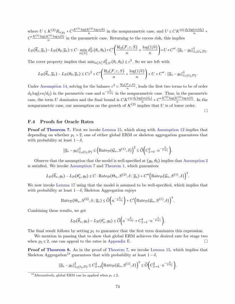
where U ≤K(2)Rn,p2 +CK(2) log(K(2) logn/δ)
n in the nonparametric case, and U ≤ CK(2) d2 log(en/d2)
n +
C ′K(2) log(K(2) logn/δ)
n in the parametric case. Returning to the excess risk, this implies
LD(θn, gn)−LD(θ0, gn) ≤ C ⋅ mini∈[N]
d2S′(θi, θ0)+C
′(H2(F , ε, S)
n+
log(1/δ)
n)+U +C ′′
⋅∥gn − g0∥4L4(`2,D).
The cover property implies that mini∈[N] d22,S′(θi, θ0) ≤ ε
2. So we are left with
LD(θn, gn) −LD(θ0, gn) ≤ Cε2+C ′
(H2(F , ε, S)
n+
log(1/δ)
n) +U +C ′′
⋅ ∥gn − g0∥4L4(`2,D).
Under Assumption 14, solving for the balance ε2 ≍H2(F ,ε,S)
n , leads the first two terms to be of order
d2 log(en/d2) in the parametric case and n− 2
2+p2 in the nonparametric case. Thus, in the parametric
case, the term U dominates and the final bound is CK(2) d2 log(en/d2)
n +C ′K(2) log(K(2) logn/δ)
n . In the
nonparametric case, our assumption on the growth of K(2) implies that U is of lower order.
F.4 Proofs for Oracle Rates
Proof of Theorem 7. First we invoke Lemma 15, which along with Assumption 12 implies thatdepending on whether p1 > 2, one of either global ERM or skeleton aggregation guarantees thatwith probability at least 1 − δ,
∥gn − g0∥2L4(`2,D) ≤ (RateD(Gn, S
(1), δ))2≤ O(C2
2→4 ⋅ n− 2
2+p1 ).
Observe that the assumption that the model is well-specified at (g0, θ0) implies that Assumption 2is satisfied. We invoke Assumption 7 and Theorem 1, which guarantees
LD(θn, g0) −LD(θ⋆n, g0) ≤ C ⋅RateD(Θn, S
(2), δ ; gn) +C′′(RateD(Gn, S
(1), δ))4.
We now invoke Lemma 17 using that the model is assumed to be well-specified, which implies thatwith probability at least 1 − δ, Skeleton Aggregation enjoys
RateD(Θn, S(2), δ ; gn) ≤ O(n
− 22+p2 ) +C ′
(RateD(Gn, S(1), δ))
4.
Combining these results, we get
LD(θn, g0) −LD(θ⋆n, g0) ≤ O(n
− 22+p2 +C4
2→4 ⋅ n− 4
2+p1 ).
The final result follows by setting p1 to guarantee that the first term dominates this expression.We mention in passing that to show that global ERM achieves the desired rate for stage two
when p2 ≤ 2, one can appeal to the rates in Appendix E.
Proof of Theorem 8. As in the proof of Theorem 7, we invoke Lemma 15, which implies thatSkeleton Aggregation19 guarantees that with probability at least 1 − δ,
∥gn − g0∥2L2(`2,D) ≤ C
22→4(RateD(Gn, S
(1), δ))2≤ O(C2
2→4 ⋅ n− 2
2+p1 ).
19Alternatively, global ERM can be applied when p1 ≤ 2.
74

Observe that since Θn is convex, Assumption 2 is satisfied, and so we can invoke Assumption 7 andTheorem 1 to get
LD(θn, g0) −LD(θ⋆n, g0) ≤ C ⋅RateD(Θn, S
(2), δ ; gn) +C′′(RateD(Gn, S
(1), δ))4.
We use global ERM for the second stage. Lemma 16 implies that since the class Θn is convex, withprobability at least 1 − δ, global ERM guarantees
RateD(Θn, S(2), δ ; gn) ≤ O(n
− 22+p2
∧ 1p2 ).
This leads to a final guarantee of
LD(θn, g0) −LD(θ⋆n, g0) ≤ O(n
− 22+p2
∧ 1p2 +C4
2→4 ⋅ n− 4
2+p1 ),
and the stated result follows by setting p1 to guarantee that the first term dominates this expression.
Proof of Theorem 9. Lemma 15 implies that either Skeleton Aggregation or global ERM (forp1 ≤ 2) guarantees that with probability at least 1 − δ,
∥gn − g0∥2L2(`2,D) = (RateD(Gn, S
(1), δ))2≤ O(n
− 22+p1 ).
Since Assumption 8 is satisfied, we appeal to Lemma 2, which guarantees
LD(θn, g0) −LD(θ⋆n, g0) ≤ C ⋅RateD(Θn, S
(2), δ ; gn) +C′′(RateD(Gn, S
(1), δ))2.
We use global ERM for the second stage. The standard Rademacher complexity bound for ERM(e.g. Shalev-Shwartz and Ben-David (2014)), states that with probability at least 1 − δ, the excessrisk is bounded by the Rademacher complexity of the target class Θn composed with the loss classas follows:
LD(θn, gn) −LD(θ⋆n, gn) ≤ 2 ⋅Eε sup
θ∈Θn
2
n
n/2
∑t=1
εt`(θ(xt), gn(wt), zt)
´¹¹¹¹¹¹¹¹¹¹¹¹¹¹¹¹¹¹¹¹¹¹¹¹¹¹¹¹¹¹¹¹¹¹¹¹¹¹¹¹¹¹¹¹¹¹¹¹¹¹¹¹¹¹¹¹¹¹¹¹¹¹¹¹¹¹¹¹¹¹¹¹¹¹¹¹¹¹¹¹¹¹¹¹¹¹¹¹¹¹¹¹¹¹¹¹¹¹¹¹¹¹¹¹¹¹¹¹¹¸¹¹¹¹¹¹¹¹¹¹¹¹¹¹¹¹¹¹¹¹¹¹¹¹¹¹¹¹¹¹¹¹¹¹¹¹¹¹¹¹¹¹¹¹¹¹¹¹¹¹¹¹¹¹¹¹¹¹¹¹¹¹¹¹¹¹¹¹¹¹¹¹¹¹¹¹¹¹¹¹¹¹¹¹¹¹¹¹¹¹¹¹¹¹¹¹¹¹¹¹¹¹¹¹¹¹¹¹¹¹
=∶Rn/2(` Θn, S(2))
+C
√log(1/δ)
n.
Using Lemma 13 and boundedness of the loss, we have
Rn/2(` Θn, S(2)
) ≤ C ⋅ infα>0
⎧⎪⎪⎨⎪⎪⎩
α + ∫1
α
√H2(` Θn, ε, S(2))
ndε
⎫⎪⎪⎬⎪⎪⎭
.
Since the loss is 1-Lipschitz with respect to `2, we have H2(` Θn, ε, S(2)) ≤H2(Θn, ε, S
(2)). Underthe assumed growth of H2(Θn, ε, S
(2))∝ ε−p2 , this gives
RateD(Θn, S(2), δ ; gn) ≤ O(n
− 12∧ 1p2 ).
This leads to a final guarantee of
LD(θn, g0) −LD(θ⋆n, g0) ≤ O(n
− 12∧ 1p2 + n
− 22+p1 .),
The theorem statement follows by setting p1 so that the first term dominates.
75

G Proofs from Section 8
Orthogonality for Treatment Effects Example (Section 8.1). We first show that Assump-tion 2 holds whenever the second stage is well-specified (i.e. θ0 ∈ Θn). We have
DθLD(θ0, g0)[θ − θ0] = −2 ⋅E[((Y −m0(X,W )) − (T − e0(W ))θ0(X))(T − e0(W ))(θ(X) − θ0(X))].
In particular, for any x we have
E[(Y −m0(X,W )) − (T − e0(W ))θ0(X))(T − e0(W )) ∣X = x]
= E[(Tθ0(W ) + f0(W ) + ε1 − e0(X)θ0(W ) − f0(W )) − (T − e0(W ))θ0(X))(T − e0(W )) ∣X = x]
= E[ε1 ⋅ ε2 ∣X = x] = E[E[ε1 ∣X = x, ε2] ⋅ ε2 ∣X = x] = 0,
and so DθLD(θ0, g0)[θ − θ0] = 0. To establish orthogonality for the propensities e, let θ, θ′ be fixed.Then we have
DeDθLD(θ,m0, e0)[θ′− θ, e − e0]
= 2 ⋅ E[((Y −m0(X,W )) − (T − e0(W ))θ(X))(θ′(X) − θ(X))(e(W ) − e0(W ))]
− 2 ⋅E[(θ(X)(T − e0(W ))(θ′(X) − θ(X))(e(W ) − e0(W )))].
To handle the first term, we use that for any x,w,
E[((Y −m0(X,W )) − (T − e0(W ))θ(X)) ∣X = x,W = w]
= E[ε1 + ε2 ⋅ (θ0(X) − θ(X)) ∣X = x,W = w] = 0.
Similarly, the second term is handled by using that
E[θ(X)(T − e0(W )) ∣X = x,W = w] = E[θ(X) ⋅ ε2 ∣X = x,W = w] = 0.
To establish orthogonality for the expected value parameter m, for any θ, θ′ we have
DmDθLD(θ,m0, e0)[θ′− θ,m −m0]
= 2 ⋅ E[(T − e0(W ))(θ′(X) − θ(X))(m(X,W ) −m0(X,W ))]
= 2 ⋅ E[ε2 ⋅ (θ′(X) − θ(X))(m(X,W ) −m0(X,W ))]
= 0,
which follows from the assumption E[ε2 ∣X,W ] = 0. Note that both of these orthogonality proofsheld for any choice of θ, not just θ0, and hence universal orthogonality holds.
Orthogonality for Missing Data Example (Section 8.4). We first show that the gradientvanishes in the sense of Assumption 2 when evaluated at θ0. In particular, for any choice of h wehave
DθLD(θ0,h, e0)[θ − θ0]
= E[(−2T(Y − θ0(X))
e0(W )− h(W )(T − e0(W )))(θ(X) − θ0(X))].
76

Using that E[T ∣W ] = e0(W ) and X ⊆W :
= E[(−2T(Y − θ0(X))
e0(W ))(θ(X) − θ0(X))].
Using that T ∈ 0,1:
= E[(−2T(Y − θ0(X))
e0(W ))(θ(X) − θ0(X))].
Using that T ⊥ Y ∣W and that X ⊆W :
= EW [(−2E[T ∣W ]E[(Y − θ0(X)) ∣W ]
e0(W ))(θ(X) − θ0(X))]
= −2E[(Y − θ0(X))(θ(X) − θ0(X))].
Using that E[Y ∣X] = θ0(X):
= 0.
To establish orthogonality with respect to e, we have
DeDθLD(θ0,h0, e0)[θ − θ0, e − e0]
= E[(2T(Y − θ0(X))
e20(W )
+ h0(W ))(θ(X) − θ0(X))(e(W ) − e0(W ))].
Using that X ⊆W :
= EW [(2(E[Y ∣W ] − θ0(X))
e0(W )+ h0(W ))(θ(X) − θ0(X))(e(W ) − e0(W ))].
The result follows immediately, using that h0(w) = −2(E[Y ∣W=w]−θ0(x))
e0(w).
= 0.
To establish orthogonality with respect to h, we have
DhDθLD(θ0,h0, e0)[θ − θ0, h − h0]
= E[(T − e0(W ))(θ(X) − θ0(X))(h(W ) − h0(W ))]
= E[ε2 ⋅ (θ(X) − θ0(X))(h(W ) − h0(W ))].
Using that E[ε2 ∣W ] = 0 and X ⊆W :
= 0.
77