organizational hierarchies in the slovenian manufacturing

Munich Personal RePEc Archive

Organizational Hierarchies in the

Slovenian Manufacturing Sector

Bonilla, Santiago and Polanec, Sašo

Universidad Santiago de Cali, University of Ljubljana

13 September 2020

Online at https://mpra.ub.uni-muenchen.de/103009/

MPRA Paper No. 103009, posted 22 Sep 2020 10:00 UTC

Organizational Hierarchies in the Slovenian

Manufacturing Sector∗

Santiago Bonilla† and Saso Polanec‡

July 8, 2020

Abstract

We study organizational hierarchies in a transition country. Using employer-employee

matched data for a set of Slovenian manufacturing firms, we find strong support for

the key hypotheses of the knowledge-based hierarchies proposed by Garicano (2000) and

Caliendo and Rossi-Hansberg (2012). According to these theories, firms should organize in

consecutively ordered layers with less hours and higher wages in higher layers. Following

Caliendo, Monte, and Rossi-Hansberg (2015b), who were the first to test the predictions

of knowledge-based theories of organizational hierarchies, we are able to directly compare

our results to those obtained for French manufacturing firms. We find that Slovenian

firms exhibit lower consistency with consecutive ordering of organizational layers, have on

average fewer organizational layers and change them less frequently. We attribute lower

organizational depth to the higher wage premia to workers in higher organizational layers,

which is an implication of under-investment in human capital during the socialist era.

Keywords: Organizational hierarchies, human capital, wages

JEL classification: D21, D24, J24, J31

1 Introduction

Firms facing decisions regarding organization of production must deal with questions like how

many and what kind of workers to hire, and what roles should they play. When facing rising

demand, firms must decide whether to replicate their operations to a larger scale or instead

reorganize their employees in teams. Similarly, when facing declining demand, they decide

∗We are grateful to the Slovenian Statistical Office for allowing us to access, use and analyze the data in a

secure room.†Faculty of Entrepreneurial and Economic Sciences, Universidad Santiago de Cali, Calle 5 # 62-00, 7600

Cali, Colombia. E-mail: [email protected]‡School of Economics and Business, University of Ljubljana, Kardeljeva pl. 17, 1000 Ljubljana, Slovenia.

E-mail: [email protected].

1

whether to reduce the number of workers, or change the organization of teams. The theories of

knowledge-based hierarchies provide nuanced answers to such questions that often depart from

traditional theory of labor demand with homogeneous workers.

In the seminal work Garicano (2000) develops a theory, which predicts that firms should orga-

nize their workforce in hierarchical layers, with the less-knowledgeable workers dedicated solely

to the most routine tasks, while the more-knowledgeable ones deal only with more complex

problems that might appear in production and give directions to the others regarding these

harder tasks.1 Caliendo and Rossi-Hansberg (2012) consider these decisions within the general

equilibrium context featuring heterogeneous firms, which allows the authors to derive further

theoretical insights that relate firm organization and its characteristics. A firm facing an in-

crease (decrease) in demand or productivity, may add (drop) layers, as having many layers

of management with more knowledgeable managers at the top, but much less knowledgeable

employees in the bottom layers, allows it to have lower production costs. Changes in the num-

ber of layers are expected only when production costs fall with adding or dropping layers. If

changes in value added are too small, firms may instead respond by changing the number of

working hours.

In this paper we investigate whether the predictions of the theoretical model developed by

Caliendo and Rossi-Hansberg (2012) also hold for Slovenian manufacturing firms. We examine

the differences between firms with different number of hierarchical layers, and investigate the

consequences of adding/dropping layers of management due to expansions/contractions in value

added, as opposed to the case when they keep the same hierarchical structure. For this purpose

we use a comprehensive annual employer-employee matched data set of Slovenian manufacturing

firms covering the period 1997–2011. Using employee-level information on ISCO 88 4-digit

occupation code, we map each worker into one of four possible hierarchical layers that each

firm can have, thus obtaining a data set that is suitable for testing the implications of the

model by Caliendo and Rossi-Hansberg (2012). In our empirical analysis we follow closely the

empirical methodology used by Caliendo et al. (2015b), who analyze employer-employee data

for French manufacturing firms, which makes many of our results directly comparable to those

reported in their paper.

Our findings mostly confirm the theory of Caliendo and Rossi-Hansberg (2012) and are aligned

with the results obtained by Caliendo et al. (2015b) for French manufacturing firms. First of

all, we observe that Slovenian firms pay higher wages in higher layers; larger firms in terms

of value added are also larger in terms of number of layers and hours of work, and pay higher

wages. Second, we find that the probability of firms adding layers increases with value added,

and that the probability of adding 1 layer is larger than that of adding more than 1 layer.

Third, we note that firms adding more layers at a certain transition period tend to grow faster

than their counterparts that diminish or preserve the same number of layers. In comparison to

French firms, Slovenian firms tend to pay higher wage premia in higher layers and have fewer

1At the core of this cost minimization decision is the trade off between increasing returns to specialization(due to economies of scale in the use of knowledge) and matching problems to workers, which gets increasinglydifficult with specialization.

2

organizational layers. We attribute these differences to relative scarcity of skilled workers in

Slovenia, a heritage of under-investment in human capital during the socialist era, particularly

in tertiary education (Bartolj, Ahcan, Feldin, and Polanec, 2013). Due to higher wage premia,

Slovenian firms have weaker incentives to add organizational layers and are thus less likely to

adjust them.

More to the point, we also explore firm dynamics in terms of hours of work and wages when

firms grow in size, both with and without changing their number of layers. When firms grow in

value added and keep the same number of layers, we observe that they hire more hours of work

and increase wages in all layers. However, according to our estimated elasticities and compared

to French firms in Caliendo et al. (2015b), we note that Slovenian firms tend to adjust more

in terms of hours of work rather than in wages. Now, when firms grow by changing their orga-

nizational structure, the patterns we find also coincide with those observed for French firms in

Caliendo et al. (2015b): firms that add (drop) a layer of management increase (decrease) hours

of work, but decrease (increase) average wages in pre-existing layers. This is fully consistent

with the theoretical prediction by Caliendo and Rossi-Hansberg (2012), as firms that decide to

add (drop) a layer of management must be, at the same time, transferring knowledge upward

(downward) by reducing (increasing) it in all layers that pre-date the corresponding transition.

Again, our estimates suggest that Slovenian firms rely relatively more heavily on hours of work

than on wages to perform said adjustments when compared to French firms.

Finally, we employ worker education and experience as more direct measures of knowledge, in

the same manner as Caliendo et al. (2015b), in order to explore how firms redistribute those

resources as they change their layer structure. Our results show that the theory holds well in

Slovenian firms: in the vast majority of cases, when undergoing transitions that add (drop)

layers of management, Slovenian firms decrease (increase) either average education or average

experience in all pre-existing layers, as they transfer knowledge to (from) the newly added

(dropped) top layers. In fact, Slovenian firms seem to transfer knowledge across layers via

worker education and experience more than average wages reveal.

The structure of the paper is as follows. Section 2 contains a brief review of the most relevant

literature on organizational hierarchies. Section 3 describes the sources of data and variables

we use in our empirical estimations and Section 4 contains summary statistics. We present our

key empirical findings in Section 5. Section 6 concludes.

2 Literature Review on Organizational Hierarchies

The study of organizations has been present in economics literature for a long time, with early

works aiming mostly to explain the distribution of pay and firm size. One of the earliest

investigations studies how managers monitor their subordinates using hierarchies (Calvo and

Wellisz, 1978). This and several subsequent studies, however, feature neither an equilibrium

approach for firms and the economy nor do they involve labor heterogeneity. Equilibrium

analysis was initially introduced in a model developed by Garicano (2000), which represents

3

a cornerstone in the theory of knowledge-based hierarchies. In his model, firms minimize the

costs of producing output by organizing their employees in teams, with the less-knowledgeable

workers dedicated solely to the most routine tasks, while the more-knowledgeable ones deal with

more complex problems that might appear in production processes. Thus, knowledge-based

hierarchies arise in the firm, with labor specialization leading to a more efficient allocation of

working time, and the organizational problem lies in determining the proper quantities and

distribution of knowledge, as well as the ways of communication within hierarchies. However,

one of the simplifying assumptions made by Garicano (2000) is that all workers have the same

learning and communication abilities. This assumption is relaxed in the models developed

by Garicano and Rossi-Hansberg (2006, 2012), which assume ex-ante heterogeneity of workers

embedded in a dynamic framework. This allows them to study the effects of communication

and information technologies on economic growth through their impact on firm organization

and innovation. Caliendo and Rossi-Hansberg (2012) use the same model of knowledge-based

hierarchies, this time allowing heterogeneity in the demand that firms face, to analyze the

effect of international trade on firm organization. By calibrating the model to U.S. data and

running simulations, they find that due to bilateral trade liberalization exporting firms will

increase the number of management layers. Hence, the theory of knowledge-based hierarchies

allows researchers to gain a better understanding of how firms organize internally, using layers

of management in order to solve the problems that emerge in the production processes. More

recently, Chen (2017) builds an industry equilibrium model in which firms use hierarchies as a

means to gain efficiency in monitoring employees in the production process. Ke, Li, and Powell

(2018) use a theoretical model based on Shapiro and Stiglitz (1984) to examine the impact of

various internal policy decisions by firms aimed at increasing worker motivation within their

ranks. One of the implications of their model is that firms tend to increase turnover rates at

top layers and create more top positions in order to keep strong promotion incentives among

workers.

In terms of empirical research, the study of organizational hierarchies in firms has been gaining

momentum, especially after the development of theories featuring worker and firm hetero-

geneity (Garicano and Rossi-Hansberg, 2006, 2012; Caliendo and Rossi-Hansberg, 2012).2 As

mentioned, this new research focuses on the effects of demand shocks, especially of foreign de-

mand shocks, foreign acquisitions, competitiveness programs, information and communication

technologies, and trade costs, on organizational hierarchies; it also studies the effects of changes

in organizational hierarchies on firm performance, like productivity and entrepreneurship.3

2Meagher (2001), using surveys of Australian employees, was one of the first to document wage premia forhigher hierarchical positions.

3Our review of empirical literature is by no means comprehensive. Bastos, Monteiro, and Straume (2018)examine the impact of foreign acquisitions on organizational structures of Portuguese firms. Tag, Astebro,and Thompson (2016) analyze the relation between Swedish firms’ hierarchical structure and the likelihoodof their former employees becoming entrepreneurs. Caliendo, Mion, Opromolla, and Rossi-Hansberg (2015a)study the effects of firm reorganizations caused by expansions on the productivity of firms. Cruz, Bussolo, andIacovone (2018) investigate the impact of competitiveness enhancing program for small and medium enterprisesin Brazil on firms’ internal organization. Bloom, Garicano, Sadun, and Van Reenen (2014) examine the impactof information technologies and communication technologies on the organizational structure of firms, whereasGumpert (2018) studies how changes in communication costs affect their organizational structure.

4

A few studies analyze the relation between organizational structures, demand shocks and wages,

in order to test the theoretical predictions by Caliendo and Rossi-Hansberg (2012). As our

work is tightly related to them, we start our survey with these studies. Tag (2013) uses linked

employer-employee data from the Swedish manufacturing sector to find that firms with more

organizational layers tend to be larger in terms of number of workers and value added, exhibit

higher wages, and when they add a new top layer of management, bottom layers experience

a decrease in average wages, whereas the opposite happens when firms drop said top layer.

Caliendo et al. (2015b) provide similar results using a comprehensive employer-employee data

set for French manufacturing firms. They provide a vast set of empirical tests that relate

organizational structure, in terms of total number of organizational layers, to firm size, in terms

of value added and working hours, and wages. For example, they compare the adjustment of

wages and hours of work in firms that change their number of layers (i.e. adding or dropping

one or more layers), as opposed to firms that keep the same number of layers across periods.

They find that firms that grow in terms of value added without changing their hierarchical

structure tend to increase wages in all layers, while firms that expand by adding one layer of

management tend to decrease average wages in pre-existing layers. As our work closely follows

theirs, we discuss their results along with ours below in order to avoid repetition.

Several recent empirical studies of organizational hierarchies exploit possibly exogenous varia-

tion in either trade costs or foreign demand. Guadalupe and Wulf (2010) analyze the impact of

increased product market competition brought by the 1989 Canada-United States Free Trade

Agreement on the depth of hierarchies and span of control in a set of large US manufacturing

firms. They find that, for a firm with average tariffs before 1989, trade liberalization induced an

increase in CEO span of control and a reduction in the number of management levels. Spanos

(2016), also using French employer-employee data for the manufacturing sector combined with

firm-transaction-level trade data, studies the relation between export performance and the or-

ganizational structure of firms. He finds a positive relationship between the total number of

organizational layers and export performance: firms with more hierarchical layers tend to sell

a greater value on average, to more destinations, and comprising a wider variety of products.

Caliendo, Monte, and Rossi-Hansberg (2017) further examine how French firms’ decisions of

becoming exporters affect their organizational structure in terms of hierarchies. These authors

find that, relative to non-exporters, exporter firms are larger, hire more hours of work, pay

higher wages and exhibit more layers of management, and, in addition, new exporters are more

likely to add new layers than non-exporters. Davidson, Heyman, Matusz, Sjoholm, and Zhu

(2017) also examine the relation between the degree of global engagement (i.e. international

commercial relations) of firms and the skill mix of the workforce they employ. Using employer-

employee data on Swedish firms, the authors find that an increase in export shares in firms has

the effect of shifting their labor structure towards more skilled personnel (i.e. professionals in

finance, sales, computing and engineering).

5

3 Data Sources and Description of Variables

3.1 Data Sources

Our empirical analysis of organizational hierarchies is conducted using data for Slovenian man-

ufacturing firms that operated during the period 1997—2011. We use three distinct data sets to

construct a matched employer-employee data set, using unique firm and individual identifiers.

Our main source of data, maintained and provided by the Slovenian Statistical Office, is the

Slovenian Employment Registry (henceforth SER), which contains information on all registered

employment contracts between employers and employees.4 The former is obliged to report ini-

tiation and termination dates of contracts, which allows us to identify the matches between

firms and workers, and to determine job tenure. Employers are also obliged to report detailed

information on occupation (4-digit ISCO 88 and ISCO 08 occupational codes), educational at-

tainment (ISCED codes), gender, hours worked, and type of employment contract (definite vs.

indefinite) for all initiated contracts and any changes to these characteristics. From the events

in the registry we construct annual data of employment spells. The most important information

for studying organizational hierarchies is the occupation of employees, which is used to allocate

workers to different organizational layers, as described in the next subsection.

The second source of data is the Slovenian Financial Authority (henceforth SFA), which collects

personal-income tax filings and also contains information on labor incomes. Unlike typical

personal-income tax data reported by employees, which lack information on the identity of

employers paying wages, we use SFA data that is reported by employers.5 Hence, the data

on gross wages used in our empirical analysis contains both personal and firm identifiers that

can be matched to employment spells. Incomes combined with employment spells allow us to

calculate the hourly gross wages that were paid to employees by individual employers.

The last source of data is the Agency of the Republic of Slovenia for Public Legal Records and

Related Services (henceforth AJPES). All registered firms are obliged to report annual balance

sheets and income statements to AJPES, from which we extract information on annual sales,

costs of material inputs and services, and total hours worked by all employees. These allow us

to calculate the measures of firm-level demand/size — value added and total hours worked.

3.2 Description of Variables

The main focus of this paper is to study how firms organize their labor into different orga-

nizational layers and how these organizations change when firms expand or contract. Hence,

it is essential to map workers with different occupations into organizational layers. We follow

4Employment contracts are registered with the Health Insurance Institute of Slovenia. The employmentregistry is maintained by the Statistical Office based on these records.

5Personal incomes reported by payees (firms, government entities etc.) were originally used for tax-inspectionpurposes, that is, to identify potential misreporting of personal incomes by individuals. More recently, thesedata have become the main source of individuals’ personal incomes, while individuals are no longer obliged tofile personal income statements.

6

Caliendo et al. (2015b) and map 4-digit ISCO 88 or ISCO 08 codes into four occupational layers

l ∈ L = {1, 2, 3, 4}, where workers in the bottom layer (layer 1) perform the ordinary tasks in

production, while higher layers deal with problems of increasing complexity. In particular, we

distinguish between:

− Occupational layer 1: blue-collar qualified and nonqualified workers (assemblers, machine

operators, drivers, laborers, office clerks, etc).

− Occupational layer 2: professionals and technicians at the supervisory level (engineers,

safety and quality inspectors, technical supervisors, etc).

− Occupational layer 3: senior staff (production and operations department managers, chief

financial officers, etc).

− Occupational layer 4: Firm owners, directors and chief executives (CEOs and general

managers).6

The mapping from occupational codes to layers is, however, not unique and depends on the

total number of occupations within a firm. For example, if a firm in a given year has employees

with occupational codes 2 and 4, then the total number of layers is L = 2, and employees with

occupational code 2 (4) belong to layer l = 1 (l = 2). So, as in Caliendo et al. (2015b) all firms

have at least 1 layer and can take the decision of adding layers, up to a maximum of 4.

Aside from the organizational layer each employee belongs to and the total number of layers in

each firm and year, the main variables we use throughout our empirical analysis are: firm-level

measures of demand/size—value added and number of working hours, and hourly gross wage

for each worker.7 Using employer and employee identifiers, we are able to construct firm-level

totals and averages per year, which we use in our empirical analysis. For the final exercise in

this paper, we also use years of formal education for each worker and use them to construct a

measure of potential experience.8

Our analysis is conducted on a sample of firms from the manufacturing sector. Namely, for

the period 1997–2008 we include firms that reported main economic activity within 2-digit

industry code 15–37, according to NACE Rev.1.9 As firms’ income statements were reported

in Slovenian Tolars prior to 2007, we convert those to Euros using a fixed exchange rate of

239.64 Tolars per Euro. In order to calculate real wages and value added, we deflate nominal

6We identify firm owners who are actually employed as managing directors using information on basis forsocial insurance.

7Note that our entire empirical analysis relies on gross wages as these are specified in employment contracts.For brevity we refer to these as wages.

8Potential years of experience (X) is calculated as X = A − T − 6, where A is age of individual, T is thenumber of years spent in formal education and 6 is the statutory school entry age in Slovenia. The number ofyears of schooling is calculated using ISCED codes of the highest completed level of education. Namely, primaryschool is given 8 years of schooling, high school is attributed 12 years of schooling, bachelor’s degree is given 16years of schooling and PhD degree corresponds to 20 years of schooling.

9During the period 2009–2011 firms reported industry codes according to NACE Rev.2 codes. We used aconcordance between the two classifications for firms entering the sample after 2008, and the NACE Rev.1 codereported in 2008 for continuing firms.

7

Table 1: Summary statistics for the sample of Slovenian manufacturing firms, 1997–2011

VariableFirm-worker-

yearObservations

Firm-yearObservations

Mean S.d.

Wage 3’302,751 71,730 5.05 2,69Total Hours 3’302,751 71,730 82,488 337,089Total Layers 3’302,751 71,730 2.28 1.01Value Added 3’302,751 71,730 1,011 6,399Experience 2’975,299 66,535 23.22 10.19Education 3’151,241 71,275 10.49 2.66

Note: This table presents the total number of firm-worker-year and firm-year observations for each variable. Meansand standard deviations are calculated from firm-level values. Firm-level values for variables that are observed atthe level of individual workers (i.e. wage, experience and education) are averages calculated at the level of firms.Value added is reported in thousands of 2004 Euros, whereas hourly wage is reported in 2004 Euros.

values using the consumer price index with base in 2004 (the year in which the exchange rate

was fixed).

We restrict our sample to employer-year observations that reported positive sales, total labor

costs and costs of materials and services, which are used to calculate value added. Due to our

focus on organizational hierarchies, we restrict the sample to firms with at least one employee.

For this set of firm-year observations we only preserve employer-employee-year observations

for which we have information on annual gross wage paid by employer to employee. The final

sample used in our empirical analysis is described in Table 1. In our main analysis we use 3.3

million firm-worker-year observations for almost 72 thousand firms. On average, these firms

paid a wage around 5 EUR (in 2004 prices), hired around 82 thousand hours of work, had on

average 2.3 total organizational layers, and produced around 1 million EUR in real value added.

The samples of observations for the two direct measures of knowledge (years of education and

potential years of experience) are slightly smaller due to missing values. Average years of

schooling and work experience for workers with available information are 10.5 and 23 years,

respectively.

4 Summary Statistics on Layers and Other Key Vari-

ables

The basic prediction of the theories of knowledge hierarchies (see Garicano (2000), Garicano

and Rossi-Hansberg (2006, 2012), and Caliendo and Rossi-Hansberg (2012)) states that in

order to minimize production costs, firms position their workers within hierarchies based on

their level of knowledge. Assuming that wages reflect the level of knowledge associated with

employees’ occupations, we should observe that workers in higher layers earn higher average

wages. Table 2 compares average hourly wages and selected percentiles of wage distributions

across layers. Evidently, higher layers are indeed associated with higher average wages and

8

wages in all percentiles of wage distributions. This finding is consistent with the evidence

reported by Caliendo et al. (2015b) for French manufacturing firms. Due to differences in

average productivity between Slovenian and French firms, direct comparisons of wages are not

meaningful.10 Instead, we compare the wage premia associated with layers in the two countries.

To calculate wage premia for French firms, we use wages reported in Table 1 in Caliendo et al.

(2015b).11 We find that the employees of Slovenian (French) firms in the fourth layer earn wages

89 (70) percent higher, on average, than the employees in the third layer. Similarly, Slovene

(French) employees in the third layer earn hourly wages 99 (80) percent higher, on average,

than those in the second layer, whereas the premium in the second layer in comparison to the

first layer is 40 (35) percent in Slovene (French) firms. These premia are significant in both

countries, although employees in Slovenian firms in the top-two layers earn significantly higher

premia than workers in French firms. In summary, wage inequality in French firms seems to

be lower than that observed in Slovenian firms, which may also affect motivation for adding

organizational layers.

Table 2: Hourly Wage Distribution by Layers

LayerAverage

Hourly Wagep.5 p.10 p.25 p.50 p.75 p.90 p.95

1 4.54 2.39 2.76 3.35 4.17 5.27 6.61 7.692 6.14 2.65 3.05 4.00 5.52 7.48 9.67 11.553 11.65 3.44 4.07 6.05 9.68 14.78 20.99 26.274 22.05 4.71 6.33 10.63 18.85 29.27 41.38 49.95

Source: Own calculations based on data from SER, SFA and AJPES.

Notes: This table presents average hourly wage and hourly wage in the corresponding percentile (in 2004Euros), by layer. We use firm-level average values as units of observation. The mean hourly wage andpercentiles in every layer are calculated for the sample of all firms and across all years of observations withinour sample.

Table 3 shows the dynamics of the number of firms and the average values of the main variables

of interest. The number of firms had been increasing until the onset of the economic crisis of

late 2008. Regarding hierarchies, the average number of layers was between 2.20 and 2.35 over

this entire period, which is slightly lower than the values reported by Caliendo et al. (2015b) for

French firms (2.51–2.60). This comparison suggests that Slovenian firms are less hierarchically

organized. This is somewhat surprising as the average number of working hours in French firms

(69–78 thousand hours) is slightly lower than that in Slovenian firms. It is also interesting

to observe that the average number of layers in Slovenia declined during the economic crisis,

falling from 2.32 in 2007 to 2.20 in 2011.

One of the main predictions of theoretical models on knowledge-based hierarchies is that larger

firms should find it optimal to choose more layers and pay higher average wages. Both of these

features are evident in our sample of firms. In Table 4 are shown averages of value added,

total hours of work and hourly wage, as well as median hourly wage, calculated separately for

10The average hourly wage of Slovenian firms is roughly one quarter of that paid by French firms.11Although Caliendo et al. (2015b) do not report wages by layers, we used average wages of five groups of

occupations, which correspond to four layers, assuming consecutively ordered layers.

9

Table 3: Dynamics of Main Variables by Year

Average

Active Number Hourly Value TotalYear firms of Layers Wage Added Hours

1997 4,007 2.27 4.09 1,056 101,6851998 4,166 2.24 4.17 987 96,5291999 4,206 2.25 4.32 1,034 97,0792000 4,404 2.27 4.39 1,052 95,3292001 4,518 2.29 4.61 1,066 90,9752002 4,674 2.33 4.73 1,070 90,5482003 4,738 2.33 4.85 1,075 87,6332004 4,823 2.35 4.88 1,026 85,2312005 4,986 2.33 5.05 1,005 81,8652006 5,138 2.32 5.26 1,049 78,5482007 5,289 2.32 5.56 1,061 74,9432008 5,443 2.30 5.70 979 73,3822009 5,378 2.24 5.58 890 67,1962010 5,222 2.21 5.80 875 64,5942011 4,738 2.20 6.01 979 65,923


Notes: The average values are calculated from the firm-level values forour sample of firms. Average value added is reported in thousand (2004)Euros and average hourly wage is given in 2004 Euros. Total hours arecalculated as the sum of hours for all employees in a firm in a given year.

10

Table 4: Description of Main Variables by Total Number of Layers

Average

Numberof

LayersFirm-Years

MedianHourly Wage

HourlyWage

ValueAdded

TotalHours

1 19,140 3.88 4.39 41.30 3,5522 22,872 4.35 4.84 182.57 17,1313 19,853 5.03 5.44 855.53 80,8994 9,865 5.65 6.05 5,125.46 390,363


Note: This table presents the number of observations (firm-years) and the average values for the referencedvariables by total number of layers. Median and average hourly wage are given in 2004 Euros, whereasaverage value added is reported in thousands of 2004 Euros.

firm-year observations with different total number of layers. While main patterns are broadly

consistent with those documented for French firms, there are some important differences. Av-

erage hourly wages in Slovenian firms monotonically increase with total number of layers, while

this is not the case for French firms.12 Namely, average hourly wage increases with total number

of layers by roughly 10 percent for Slovenian firms, whereas in France, it is the highest for firms

with only one layer, and increases modestly between firms with 2–4 layers. We attribute this

difference to the higher wage premia for higher layers, which we have discussed above, and is

related to the relative scarcity of college educated persons who are the predominant group of

workers in the third and fourth layers.13

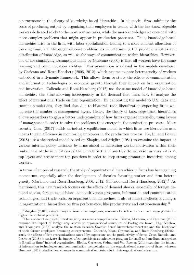
Figures 1, 2 and 3 present kernel density plots of the distributions for value added, total hours of

work and average hourly wage (all in logs), for 1-, 2-, 3- and 4-layered firms. We follow the same

procedure as Caliendo et al. (2015b), and report densities for both raw data and transformed

variables after removing year and industry fixed effects. In Figure 1 we again see how firms

with more layers of management are also larger in terms of value added, even after controlling

for year and industry fixed effects. In addition, Figure 2 shows that firms with more layers

also tend to hire more hours of work. The relation between average hourly wage and number

of layers in the firm, as presented in Figure 3, appears less striking, although more layers are

clearly related to higher wages. These distributions for Slovenian firms exhibit qualitatively

similar patterns for French firms in measures of firm size (value added and total hours), while

the distributions for average hourly wages bear some important differences. Wage distributions

in Slovenian firms are less skewed and feature thinner upper tails than in French firms. French

one-layered firms exhibit particularly a thick upper tail, which may explain the non-monotonic

ranking of average hourly wages in France.

12The rankings of median hourly wage, however, hold also for French firms.13Bartolj et al. (2013) show that Slovenia had relatively poor educational attainment at the start of the

economic transition from socialist to market economy, which leads to relatively high returns to college degreesduring the period 1994–2008, a period that partly overlaps with our sample.

11

Figure 1: Distribution of Value Added by Total Number of Layers.


Notes: This figure depicts the distribution of logarithm of value added by total number of layers. Theleft panel uses raw data in order to estimate kernel densities by groups of firm-year observations with thesame number of layers. The right panel shows the distributions of value added after we remove year andindustry fixed effects. To do so, we run a linear regression of the logaritm of value added on indicatorvariables for the number of layers in the firm, the two-digit NACE industry codes, and the year. We takefirms with 1 layer of management in Food and Beverage Production (2-digit code 15) in the year 1997as the base group. Then, we use the residuals of the previous regression, the median value added for thebase group and the estimated coefficients for the number of layer dummies in order to estimate the logvalue added free of industry and year fixed effects. Finally, we compute the kernel-density estimates forthe distribution of our log value added estimates, using the number of layers of each firm as the groupingvariable.

Figure 2: Distribution of Working Hours by Total Number of Layers.


Notes: This figure presents kernel density estimates of the distribution of (log) working hours by totalnumber of layers. The left panel uses raw data, whereas the right panel uses hours after removing industryand year fixed effects. To build it we use the same methodology as in Figure 1, after computing totalworking hours used in each firm-year.

5 The Empirics of Organizational Hierarchies in Slove-

nia

5.1 Consecutively Ordered Layers and Hierarchical Behavior

Next, we analyze layer management in Slovenian manufacturing firms. Specifically, we test

whether firms’ behavior is consistent with theoretical predictions by Caliendo and Rossi-Hansberg

(2012) regarding the choices of number of hours in different layers, and how wages and working

hours change when firms choose to add layers. The first prediction states that hours in layers

12

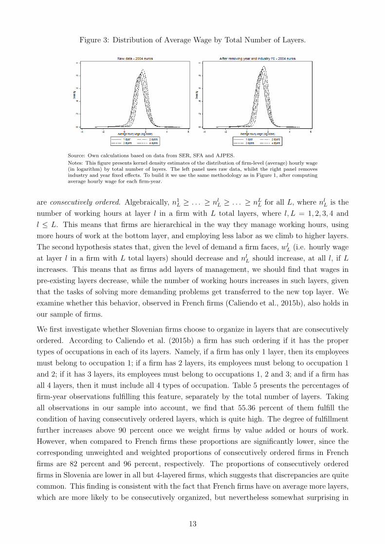
Figure 3: Distribution of Average Wage by Total Number of Layers.


Notes: This figure presents kernel density estimates of the distribution of firm-level (average) hourly wage(in logarithm) by total number of layers. The left panel uses raw data, whilst the right panel removesindustry and year fixed effects. To build it we use the same methodology as in Figure 1, after computingaverage hourly wage for each firm-year.

are consecutively ordered. Algebraically, n1L ≥ . . . ≥ nl

L ≥ . . . ≥ nLL for all L, where nl

L is the

number of working hours at layer l in a firm with L total layers, where l, L = 1, 2, 3, 4 and

l ≤ L. This means that firms are hierarchical in the way they manage working hours, using

more hours of work at the bottom layer, and employing less labor as we climb to higher layers.

The second hypothesis states that, given the level of demand a firm faces, wlL (i.e. hourly wage

at layer l in a firm with L total layers) should decrease and nlL should increase, at all l, if L

increases. This means that as firms add layers of management, we should find that wages in

pre-existing layers decrease, while the number of working hours increases in such layers, given

that the tasks of solving more demanding problems get transferred to the new top layer. We

examine whether this behavior, observed in French firms (Caliendo et al., 2015b), also holds in

our sample of firms.

We first investigate whether Slovenian firms choose to organize in layers that are consecutively

ordered. According to Caliendo et al. (2015b) a firm has such ordering if it has the proper

types of occupations in each of its layers. Namely, if a firm has only 1 layer, then its employees

must belong to occupation 1; if a firm has 2 layers, its employees must belong to occupation 1

and 2; if it has 3 layers, its employees must belong to occupations 1, 2 and 3; and if a firm has

all 4 layers, then it must include all 4 types of occupation. Table 5 presents the percentages of

firm-year observations fulfilling this feature, separately by the total number of layers. Taking

all observations in our sample into account, we find that 55.36 percent of them fulfill the

condition of having consecutively ordered layers, which is quite high. The degree of fulfillment

further increases above 90 percent once we weight firms by value added or hours of work.

However, when compared to French firms these proportions are significantly lower, since the

corresponding unweighted and weighted proportions of consecutively ordered firms in French

firms are 82 percent and 96 percent, respectively. The proportions of consecutively ordered

firms in Slovenia are lower in all but 4-layered firms, which suggests that discrepancies are quite

common. This finding is consistent with the fact that French firms have on average more layers,

which are more likely to be consecutively organized, but nevertheless somewhat surprising in

13

the light of the Slovenian socialist heritage, which featured large hierarchies.14 It suggests that

particularly new firms tend to deviate from the hypothesized consecutive ordering. Further

inspection of the data shows that main departures are primarily related to the classification of

managers/executives in small firms, who may be the only employee in firms (and often perform

multiple tasks), or may directly manage employees in the first layer. These may be considered

as misclassified, as the tasks of such managers may not correspond to those in the top layer.15

Table 5: Firm-Year Observations with Consecutively Ordered Layers

Firm-Year Observations With

1 Layer 2 Layers 3 Layers 4 Layers All obs.

Unweighted 49.27 56.18 38.12 100 55.36Weighted by Value Added 62.17 79.27 72.62 100 91.98Weighted by Hours of Work 68.30 80.84 72.66 100 90.95


Notes: This table presents the percentages of firm-year observations that fulfill the condition of having consec-utively ordered layers, where observations were grouped by number of layers. We also present the percentagesof fulfillment, weighted by value added and by total hours of work hired.

Next, we examine whether firms exhibit hierarchical behavior with respect to the total hours

of work they hire. According to the aforementioned theory, a firm with L total layers satisfies

a hierarchy in hours between layers l and l + 1, with l = 1, . . . , L− 1, if the number of working

hours employed in layer l is larger or equal than the hours of work hired in layer l + 1. For

instance, a firm with 4 layers satisfies all hierarchies in hours of work if it hires more hours of

work in the bottom layer than in the second layer, more hours of work in the second layer than

in the third one, and more hours of work in the third layer than in the top layer.

Table 6 shows that the majority of firms in our sample satisfy hierarchical behavior with respect

to hours of work. For instance, more than 71% of firms with 4 layers of management satisfy

hierarchical order in all of their layers.16 Slovenian firms with 3 and 4 layers—in comparison

to French firms (Caliendo et al., 2015b)—tend to exhibit higher shares of firms with consistent

ranking (based on all layers) by 8 and 14 percentage points, respectively, whereas in firms with

only 2 layers the percentage is lower by 5 points. These numbers suggest that larger firms in

particular tend to strongly comply with hierarchical patterns for hours.

Regarding hierarchical patterns for wages — according to Caliendo et al. (2015b) — a firm

with total number of layers L satisfies a hierarchy in wages between layers l and l + 1, if the

average wage in layer l + 1 is higher than or equal to the average wage in layer l. The results in

Table 7 suggest that firms do exhibit such hierarchies regarding wages, albeit the percentage of

14We also investigated a subsample of firms with socialist heritage, defined as those that existed already priorto 1988—a year of deregulation of entry of privately-owned firms—and find them to be larger, to have fourlayers and thus to fully comply with the consecutive ordering of layers. The share of such firms (including theirspin offs) is, however, relatively small in comparison to post-1988 entrants.

15Note that employers can select only one occupation in the registration forms for each employee, which maynot fully correspond to the actual job description.

16The numbers are even higher when the percentages are weighted by firm value added. These are omittedfor brevity, but available upon request.

14

Table 6: Firm-Year Observations with Hierarchies in Terms of Hours

Number ofLayers

N lL ≥ N l+1

L

For all lN1

L ≥ N2L N2

L ≥ N3L N3

L ≥ N4L

2 81.72 81.72 ... ...3 72.23 84.40 87.06 ...4 71.24 88.71 96.26 82.94


Note: This table presents the percentages of firms that fulfill the condition of having hierarchies interms of working hours. A firm satisfies a hierarchy in hours between layers l and l + 1 if the numberof working hours in layer l is at least as large as the number of working hours in layer l + 1. Thesecond column reports the percentage of firms that satisfy hierarchies in hours at all layers at once,while columns 3 to 5 report this only at layer l = 1, 2, 3. The percentages are presented accordingto the number of layers in the firm, as the first column indicates.

4-layered firms satisfying this condition in all layers is not as high as it is regarding hierarchies

in hours of work. In comparison to French firms these numbers tend to be similar in 3-layered

firms, but higher (lower) in 4 (2)-layered firms.

Table 7: Firm-Year Observations with Hierarchies in Terms of Wages

Number ofLayers

wl+1L ≥ wl

L

For all lw2

L ≥ w1L w3

L ≥ w2L w4

L ≥ w3L

2 73.68 73.68 ... ...3 62.61 75.15 85.40 ...4 64.34 91.52 88.15 80.84


Note: This table presents the percentages of firms that fulfill the condition of having hierarchies inwages. A firm satisfies a hierarchy in wages between layers l + 1 and l if the average wage in layerl+1 is at least as large as the average wage in layer l. The second column reports the percentage offirms that satisfy hierarchies in wages at all layers simultaneously, while columns 3 to 5 report thisonly at layer l = 1, 2, 3. The percentages are presented according to the number of layers in the firm,as the first column indicates.

The hierarchical organization within firms can also be presented graphically. Figure 4 presents

a clearer view of the hierarchies of 1-, 2-, 3- and 4-layered firms in terms of normalized average

hours of work (normalized by total hours in the top layer) and average wages. We can infer

that firms use more hours of work in lower layers and pay lower average wages. As we move

upward in the hierarchy, firms use less hours of work and pay higher average wages.

The fact that firms organize employees with different levels of knowledge into different hierar-

chies, as described above, should also be reflected in wage inequality across layers within firms.

Namely, it should increase as they add new layers of management (see Garicano and Rossi-

Hansberg (2006)). To investigate that, we follow the method used by Caliendo et al. (2015b).

We regress the log-hourly wage of workers in each firm-year on a constant and dummy vari-

ables for all layers (excluding layer 1), extract the R2, and compute the mean across all firms,

15

Figure 4: Firm Hierarchies Normalized by Hours in the Top Layer

Source: Own calculations based on data from SER, SFA and AJPES.Note: This figure presents hierarchies of the average firm with L = 1, 2, 3, 4 layers. Following Caliendoet al. (2015b), we only use data for the middle tercile of firm-year observations according to value added,and for each group of firms with L = 1, 2, 3, 4 layers we compute average hours of work and average wageat every layer. We normalize average number of hours by dividing them by their value at the top layer.The x-axis measures normalized average hours of work in the L-layered firm at layer l = 1, ..., L, whilethe y-axis measures average hourly wage (in 2004 Euros) at each layer.

grouping firms by number of total layers. Hence, for each firm-year i = 1, . . . , N we estimate:

logwi,j = αi +L∑

l=2

βi,lDi,j,l + ǫi,j (1)

where logwi,j is the log hourly wage of employee j in firm-year i, and Di,j,l is a dummy variable

for employee j in firm-year i in layer l, which takes the value of 1 if the employee in a given

firm-year pair belongs to layer l, and zero otherwise. We also compute the mean R2 using hours

of work and value added as weights of observations with different numbers of layers.

Our results, reported in Table 8, show that cross-layer wage variation explains almost 43% of

mean wage variation in Slovenian firms. When weighing these proportions of variations by hours

hired or value added, the share of mean wage variation explained by cross-layer variation falls

to around 30%, which suggests there is a negative relation between firm size (captured by hours

of work and value added) and variance of wages due to layer variation. These percentages are

lower in comparison to French firms, for which Caliendo et al. (2015b) report that cross-layer

variation explains around 50% of unweighted and weighted mean wage variation.

16

Table 8: Average Share of Wage Variation Explained by Layer Variation

Weighted by

Firm-Years UnweightedHoursof Work

ValueAdded

All Firms 58,700 42.86 29.12 30.21Firms with More than 1 Layer 52,052 48.33 29.34 30.42Firms with 1 Layer 6,648 0.00 0.00 0.00Firms with 2 Layers 22,361 51.85 26.62 28.83Firms with 3 Layers 19,826 48.17 29.59 31.17Firms with 4 Layers 9,865 40.68 29.52 30.29


Note: This table presents the mean R2, across all firms and grouped by total number of layers, resulting from the regressionlogwi,j = αi+

∑Ll=2

βi,lDi,j,l+ǫi,j , for each firm-year i = 1, . . . , N , where logwi,j is the log hourly wage of employee j in firm-yeari, and Di,j,l is a dummy variable for employee j in firm-year i in layer l, which takes the value of 1 if said employee in said firm-yearbelongs to layer l, and zero otherwise. Thus, R2 is a measure of wage variation due only to layer variation within firms. We alsocompute the weighted mean R2 across firm-years, using hours of work and value added as weights. We should note that, for firmswith 1 layer, there is no wage variation across layers since there is only one of them.

5.2 Firm Size and Layer Transitions

In this section we investigate firms’ transitions in terms of number of layers. Using the method

employed by Caliendo et al. (2015b), we compute the share of firms that, conditioned on having

L layers in a certain year, add/drop, keep the same number of layers, or exit the sample in the

next year.

According to Table 9, the majority of Slovenian firms—between 76 and 83 percent of them—

in any given year tend to keep their number of layers unaltered until the next year, which

means their hierarchical structure is slightly more rigid than that of their French counterparts,

for which values around 62–71 percent were reported (Caliendo et al., 2015b). While lower

transition probabilities may be partly related to higher exit rates among French firms, a higher

rigidity of layers in Slovenia is still observed even when we consider transition probabilities

for surviving firms alone. Table 9 also reveals that, similar to French firms, the exit rates for

Slovenian firms also decline with total number of layers, which is consistent with the commonly

observed fact that exit rates decline with firm size. Finally, Table 9 shows that when Slovenian

firms decide to expand or contract their size in terms of layers, they do so by adding or dropping

only one layer: transitions that add or drop more than one layer are not very likely.

Next we investigate how the probability of adding/dropping layers varies with firm size, mea-

sured in terms of value added. The theory by Caliendo and Rossi-Hansberg (2012) states that

some firms will add new layers of management when receiving positive demand shocks and/or

productivity improvements, and the probability of this happening is higher for firms with higher

value added. Hence, a positive relation between value added and the probability of adding lay-

ers should be observed. To provide descriptive evidence that supports this prediction, Figure

5 presents a lowess smoothing interpolation of the fraction of firms that change their number

of layers as a function of their value added, conditioned on the initial number of layers of the

17

Table 9: Layer Transition Matrix

Number of Layers at t+ 1

Number ofLayers at t

Exit 1 2 3 4 Total

1 10.43 77.06 11.40 1.05 0.06 1002 6.34 8.37 75.95 8.94 0.39 1003 4.75 0.95 9.66 78.73 5.91 1004 4.19 0.28 1.03 11.43 83.08 100


Note: This table presents the proportion of firms, among all firm-years, that condi-tioned on having L = 1, 2, 3, 4 layers in year t, decide to change/keep their hierarchicalstructure or exit the market in year t+ 1.

firm, following the same method used by Caliendo et al. (2015b). Supporting the theory by

Caliendo and Rossi-Hansberg (2012), Figure 5 shows that the probability of adding layers for

Slovenian firms increases with value added, and that the probability of adding only one layer

is always greater than that of adding more than one. At the same time, the probability of

dropping layers decreases with value added. A visual inspection suggests that the behavior of

Slovenian and French firms is very similar (Caliendo et al., 2015b).

Figure 5: Transitions Between Layers and Value Added

Source: Own calculations based on data from SER, SFA and AJPES.Note: This figure presents lowess smoothing interpolations of the fraction of firms that change theirnumber of layers as a function of their value added, conditional on the initial number of layers of thefirm. The x-axis measures value added (in 2004 Euros), while the y-axis measures the fraction of firmswith L = 1, 2, 3, 4 layers engaging in the respective layer transitions in the next year. We follow Caliendoet al. (2015b) in allocating groups of firm-years (by their total number of layers L) into 100 bins, accordingto their value added. Then, we compute in each bin the share of firm-years that engage in each type oflayer transition in the next year. Finally, we graph the lowess plot of the fraction of firm-years in eachtype of transition against the average value added in each bin, for all bins.

18

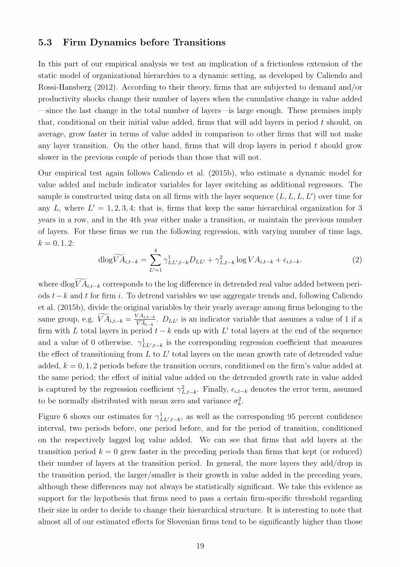
5.3 Firm Dynamics before Transitions

In this part of our empirical analysis we test an implication of a frictionless extension of the

static model of organizational hierarchies to a dynamic setting, as developed by Caliendo and

Rossi-Hansberg (2012). According to their theory, firms that are subjected to demand and/or

productivity shocks change their number of layers when the cumulative change in value added

—since the last change in the total number of layers—is large enough. These premises imply

that, conditional on their initial value added, firms that will add layers in period t should, on

average, grow faster in terms of value added in comparison to other firms that will not make

any layer transition. On the other hand, firms that will drop layers in period t should grow

slower in the previous couple of periods than those that will not.

Our empirical test again follows Caliendo et al. (2015b), who estimate a dynamic model for

value added and include indicator variables for layer switching as additional regressors. The

sample is constructed using data on all firms with the layer sequence (L,L, L, L′) over time for

any L, where L′ = 1, 2, 3, 4; that is, firms that keep the same hierarchical organization for 3

years in a row, and in the 4th year either make a transition, or maintain the previous number

of layers. For these firms we run the following regression, with varying number of time lags,

k = 0, 1, 2:

dlogV Ai,t−k =4∑

L′=1

γ1LL′,t−kDLL′ + γ2

L,t−k log V Ai,t−k + ǫi,t−k. (2)

where dlogV Ai,t−k corresponds to the log difference in detrended real value added between peri-

ods t−k and t for firm i. To detrend variables we use aggregate trends and, following Caliendo

et al. (2015b), divide the original variables by their yearly average among firms belonging to the

same group, e.g. V Ai,t−k =V Ai,t−k

V At−k. DLL′ is an indicator variable that assumes a value of 1 if a

firm with L total layers in period t− k ends up with L′ total layers at the end of the sequence

and a value of 0 otherwise. γ1LL′,t−k is the corresponding regression coefficient that measures

the effect of transitioning from L to L′ total layers on the mean growth rate of detrended value

added, k = 0, 1, 2 periods before the transition occurs, conditioned on the firm’s value added at

the same period; the effect of initial value added on the detrended growth rate in value added

is captured by the regression coefficient γ2L,t−k. Finally, ǫi,t−k denotes the error term, assumed

to be normally distributed with mean zero and variance σ2k.

Figure 6 shows our estimates for γ1LL′,t−k, as well as the corresponding 95 percent confidence

interval, two periods before, one period before, and for the period of transition, conditioned

on the respectively lagged log value added. We can see that firms that add layers at the

transition period k = 0 grew faster in the preceding periods than firms that kept (or reduced)

their number of layers at the transition period. In general, the more layers they add/drop in

the transition period, the larger/smaller is their growth in value added in the preceding years,

although these differences may not always be statistically significant. We take this evidence as

support for the hypothesis that firms need to pass a certain firm-specific threshold regarding

their size in order to decide to change their hierarchical structure. It is interesting to note that

almost all of our estimated effects for Slovenian firms tend to be significantly higher than those

19

reported by Caliendo et al. (2015b) for French firms. In order to illustrate this point, consider

firms with 3 layers before transition and lag 0 in both countries. Slovenian firms that shifted

to 2 (4) layers had a productivity growth 20 (10) percentage points lower (higher) than those

that kept 3 layers, whereas the corresponding French firms that shifted to 2 (4) layers had a

less than 10 (less than 5) percentage points lower (higher) value added growth than those that

kept 3 layers. This comparison suggests that Slovenian firms require a greater (relative) change

in value added in order to adjust their total number of layers, which is consistent with the

fact that Slovenian firms tend to have flatter organizations with a smaller average number of

organizational layers.

Figure 6: Growth in Value Added before and at Transition Period

Source: Own calculations based on data from SER, SFA and AJPES.Notes: This figure displays the estimates of regression coefficients γ1

LL′,t−k(and their 95 percent

confidence interval in each case) corresponding to indicator variables for various layer transitions (fromL = 1, 2, 3, 4 to L′ = 1, 2, 3, 4 number of layers). These coefficients are obtained from a dynamic equation

for real value added: dlogV Ai,t−k =∑

4L′=1

γ1LL′,t−k

DLL′ +γ2L,t−k

log V Ai,t−k+ ǫi,t−k. The coefficient

estimates are reported for k = 0, 1, 2 periods before layer transition for each group of firms, according totheir number of layers before the transition.

5.4 Changes in Hours and Wages as Firms Expand or Contract

One of the theoretical implications of the model by Caliendo and Rossi-Hansberg (2012) is

that, for firms that do not change their hierarchical structure, demand and productivity shocks

increasing (decreasing) their revenues should increase (decrease) their hours of work and wages

in all layers. Hence, in this section we analyze the changes that occur within different layers

of management in firms as they expand or contract in terms of firm size. We first investigate

the relation between real value added and normalized hours (normalized with respect to the

number of hours employed in the top layer), for those firms that keep the same number of layers

for two consecutive years. Specifically, we estimate the following equation

dlognlLi,t = βl

LdlogV Ai,t + ǫi,t, (3)

20

Table 10: Elasticities of Normalized Working Hours With Respect to Value Added, for Firmsthat Keep L Layers in Two Consecutive Years

Number ofLayers

Layer βlL

StandardError

p-Value Observations

2 1 0.108 0.009 0.000 15,9253 1 0.139 0.008 0.000 14,5253 2 0.129 0.010 0.000 14,5254 1 0.152 0.013 0.000 7,6664 2 0.135 0.014 0.000 7,6664 3 0.107 0.016 0.000 7,666


Note: This table shows our estimates of the elasticity of working hours to value added, βlL. These

estimates are obtained from the equation dlognlLi,t

= βlLdlogV Ai,t + ǫi,t, where dlognl

Li,tis the

yearly log difference in detrended normalized hours of work, in layer l and total number of layers L,

and d log V Ai,t is the yearly log difference in detrended value added, both for firm i in year t.

Here dlognlLi,t denotes log difference of detrended normalized hours of work in layer l for firm i

and period t, keeping L total layers, whereas dlogV Ai,t denotes log difference in detrended real

value added for the same firm-year observation. βlL denotes the elasticity of normalized hours

of work in layer l for firms with L layers, with respect to value added, for firms that do not

change layers in 2 consecutive years. Detrended normalized hours and value added are defined

as: nlLi,t =

nlLi,t

ntand V Ai,t =

V Ai,t

V At, where nt and V At are yearly average hours and value added,

respectively.

Our estimates for the elasticity of hours of work with respect to value added, βlL, are shown in

Table 10. We can see that, when firms grow in value added, they hire more hours of work in

all layers, i.e. our estimates of βlL are all positive and significant in all cases. We also find that,

given the total number of layers in the firm, the increase in hours of work hired is higher in

lower layers. Our estimates of βlL also satisfy that βl

L > βl′

L for l < l′, so that as firms grow in

value added, they become flatter, employing proportionally more hours of work in the bottom

layers. Comparing our results to those for French firms (Caliendo et al., 2015b), we observe that

the elasticities for Slovenian firms tend to be significantly higher. Namely, the range of these

elasticities for French firms is between 0.013 and 0.107, while the corresponding elasticities for

Slovenian firms are between 0.107 and 0.152. This finding seems expected given our previous

result that Slovenian firms are less inclined to change their organizational layers in response to

changes in value added. Moreover, a comparison of the range of estimated elasticities between

the two countries also suggests important differences in the adjustment of the number of hours

across layers, as Slovenian firms exhibit a weaker flattening of organizational hierarchies.

Next, we use a similar estimation equation, only this time to estimate the elasticity of average

wages to value added for firms keeping the same number of layers in two consecutive years. We

estimate

dlogwlLi,t = γl

LdlogV Ai,t + ǫi,t, (4)

21

Table 11: Elasticities of Wages with Respect to Value Added, for Firms that Keep L Layers inTwo Consecutive Years

Number ofLayers

Layer γlL

StandardError

p-Value Observations

1 1 0.065 0.005 0.000 13,0452 1 0.051 0.004 0.000 15,9252 2 0.068 0.005 0.000 15,9253 1 0.039 0.004 0.000 14,5253 2 0.043 0.005 0.000 14,5253 3 0.058 0.005 0.000 14,5254 1 0.019 0.004 0.000 7,6664 2 0.022 0.005 0.000 7,6664 3 0.039 0.008 0.000 7,6664 4 0.052 0.009 0.000 7,666


Note: This table presents our estimates of the elasticity of average wage to value added, γlL, for firms

that do not change layers in 2 consecutive years. The estimates are obtained from the regression

dlogwlLi,t

= γlLdlogV Ai,t + ǫi,t, where dlogwl

Li,tis the yearly log difference in detrended normalized

average wage in layer l for firm i keeping L total layers for 2 consecutive years, and d log ˜V Ai,t isthe yearly log difference in detrended value added for firm i at year t.

where dlogwlLi,t denotes the yearly log difference in detrended average wage in layer l for firm

i keeping L total layers for two consecutive years, and log V Ai,t is the yearly log difference in

detrended value added for firm i at year t. γlL denotes the elasticity of average wage in layer

l for firms with L layers with respect to value added, for firms that do not change layers in 2

consecutive years.

Table 11 presents our estimates for the elasticity of wages with respect to value added, γlL.

These results are again in line with the theory by Caliendo and Rossi-Hansberg (2012), as all

of our estimates are significant, positive, and satisfy that γlL < γl′

L for l < l′. This means

that, as firms grow in value added without adding layers, they increase wages in all their

existing layers, although the increases are proportionally larger at higher layers. Comparing

these results with those obtained for French firms (Caliendo et al., 2015b), we again observe

important differences. Wage elasticities for Slovenian firms are relatively small, ranging between

0.019 and 0.068, whereas the corresponding elasticities for French firms are significantly higher,

between 0.077 and 0.217. Interpreting these results jointly with our results on the elasticities

of hours, we can deduce that among firms that keep layers unchanged, Slovenian firms tend to

primarily adjust hours, whereas French firms mainly adjust wages.

Next, we consider the adjustment of firms depending on whether they decrease, increase, or

keep the same number of layers of management over consecutive years. The implications of

the theory by Caliendo and Rossi-Hansberg (2012) are now different than in the previous case.

Firms that grow by adding a new top layer of management should hire more hours of work,

but at the same time decrease wages in all pre-existing layers. Table 12 presents our estimates

for the average differences in log of total hours of work, normalized total hours of work, value

22

added and average firm wage, both including and excluding wages in the newly added/dropped

layer, if so. It shows that, over consecutive years, and even after removing time trends in the

variables, firms tend to increase their number of working hours, value added and wages when

adding layers. This general pattern is consistent with that documented by Caliendo et al.

(2015b) for French firms.

The same pattern is evident with respect to working hours and value added even when con-

sidering only firms that increase or do not change their number of layers. However, we find

that on average firms that increase their number of layers also tend to increase their wages,

whilst the theory implies that firms that add a layer of management should decrease wages in

bottom layers, since they are reducing knowledge in all pre-existing layers and adding a new

top layer in order to deal with uncommon problems. That is the reason why we also compute

the average log change in wages only for common layers, i.e. those which firms had both before

and after the change. The negative and significant estimates for firms that increase their total

layers show that, in accordance with the theory, wages in all pre-existing layers tend to decrease

once a firm adds a new top layer. On the contrary, when firms do not change layers or drop a

top layer, wages in all pre-existing layers tend to increase. Once again it is necessary to point

out the difference in adjustment of wages and hours between Slovenian and French firms. The

former exhibit larger changes in total hours in response to changes in the number of layers17,

whereas the latter tend to make greater wage adjustments. A case in point are firms that

expand layers. For these firms we observe that (i) the average growth rate of detrended total

hours is 0.336 for Slovenian firms and only 0.04 for French firms and (ii) the wage growth rate

in common layers is -0.059 for Slovenian firms, while the corresponding value for French firms

is -0.101.

Next, we investigate a theoretical prediction stating that firms adding layers should increase

their hours of work in all pre-existing layers and decrease wages in all pre-existing layers. This

is done in Table 13, which shows the average changes in log hours of work and wages for firms

that make a transition from L to L′ total layers (for L 6= L′), layer by layer. We focus on firms

that experience a layer transition as described by the first two columns, and we calculate the

average log change in detrended normalized hours and wages in the (common) layer (stated in

the third column). Focusing first on working hours, we confirm the theory as all our estimates

are statistically significant, and for transitions with an increase (decrease) in the total number

of layers the change is positive (negative). In comparison to French firms, we find that most

(but not all) of the absolute values of the changes we observe are lower, which is exactly what

we observed in Table 12 in the case of normalized working hours.

Regarding the adjustment of average wages to layer transitions, we note that the estimated

coefficients are not all significant as in the case of working hours. Namely, out of 20 estimates,

12 are statistically significant (at the 1% level). More importantly, among the significant

coefficients 11 out of 12 have the sign that is in line with the theory: in firms that add layers,

wages tend to decrease in every pre-existing layer, and in firms that drop layers, wages should

17Note that the adjustment of normalized hours is smaller in Slovenia, which may be due to smaller absolutechange in the top layer.

23

Table 12: Firm-Level Outcomes Conditioned on Layer Management

All Increase in LNo Change

in LDecrease in L

dlog Total Hours 0.045** 0.387** 0.043** -0.299**Detrended - 0.336** -0.003 -0.344**

dlog Normalized Hours 0.012** 1.078** 0.003 -1.046**Detrended - 1.066** -0.009** -1.058**

dlog Valued Added 0.020** 0.242** 0.012** -0.136**Detrended - 0.222** -0.008* -0.116**

dlog Average Wage 0.021** 0.034*** 0.020** 0.020**Detrended - 0.013** -0.001 0.000

Common layers 0.021** -0.037** 0.020** 0.088**Detrended - -0.059** 0.000 0.067**

% of Firms 100.00 8.34 84.01 7.66% Value Added Change 100.00 15.78 96.28 -12.06


Note: This table reports changes in various firm outcomes, grouping firms according to the type of transitionthey experience between two years: increase in their total number of layers L, decrease in L, no change in L,and altogether. For changes in the average wage in common layers, we compute average wage only taking intoaccount the layers that existed both before and after the referenced transition. To detrend variables, we again useaggregate trends following Caliendo et al. (2015b), as we explained above. In the last two rows, % of firms shows thepercentage of firms engaging in each type of transition, and % value added change shows the share of total changein value added for the whole data set explained by firms in each type of transition. ***, ** and * denote statisticalsignificance at 1, 5 and 10 percent, respectively.

increase in every pre-existing layer. In comparison to French firms, for which Caliendo et al.

(2015b) find all coefficients correctly signed and statistically significant, Slovenian firms again

exhibit lower responsiveness of wages to layer transitions.

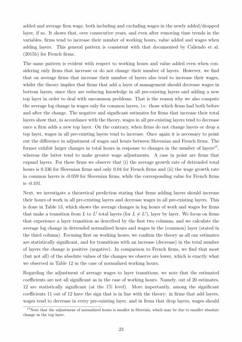
Continuing with the analysis of layers and wages, we follow Caliendo et al. (2015b) to decompose

firm-level the log-change in detrended average wage in the firm:

dlogwLi,t = log wL′i,t+1 − log wLi,t = log

[(wl≤L

L′i,t+1

wLi,t

)s+

(wL′

L′i,t+1

wLi,t

)(1− s)

]. (5)

Here wl≤LL′i,t+1 denotes the average detrended wage in all pre-existing layers in the firm after the

transition from L to L′ total layers, where L′ > L. wL′

L′i,t+1 is the average wage in the newly

added layer, wLi,t is the average wage in the firm before the transition for all layers, and s is

the share of working hours in pre-existing layers.

In Table 14 we report estimates for each component, separately by layer transitions. The upper

left and right cells show average ratios that compare wages after and before transitions in

common organizational layers. For example, for firms expanding from 1 layer to 2 layers, this

ratio is 0.987 for workers that stayed in layer 1, which implies a modest reduction of average

wage in common layers, as predicted by the theory of organizational hierarchies. Similarly,

all reorganizations that add one layer also exhibit a decrease in the average wage. However,

additions of more than one layer lead to growth in wages even in the common layers. These

24

Table 13: Average Change in Log-Hours and Log-Wages in Layer l, Conditioned on TransitionType

Total LayersBefore

Total LayersAfter

Layer dlognlLi,t S.E. dlogwl

Li,t S.E. Observations

1 2 1 0.515*** 0.039 -0.080*** 0.011 19041 3 1 0.833*** 0.137 -0.044 0.049 1651 4 1 2.621*** 0.522 0.496 0.384 92 1 1 -0.610*** 0.037 0.083*** 0.013 16322 3 1 0.645*** 0.038 -0.026*** 0.007 18482 3 2 0.383*** 0.041 -0.208*** 0.012 18482 4 1 1.442*** 0.235 0.050 0.051 772 4 2 1.581*** 0.183 -0.054 0.065 773 1 1 -0.964*** 0.120 0.118** 0.049 1503 2 1 -0.629*** 0.035 0.037*** 0.009 17423 2 2 -0.523*** 0.037 0.252*** 0.014 17423 4 1 0.770*** 0.039 0.002 0.006 10743 4 2 0.753*** 0.042 -0.047*** 0.010 10743 4 3 0.449*** 0.048 -0.213*** 0.019 10744 1 1 -1.846*** 0.432 -0.074 0.270 224 2 1 -1.540*** 0.209 -0.004 0.048 834 2 2 -1.466*** 0.186 0.225*** 0.081 834 3 1 -0.742*** 0.038 -0.006 0.008 10334 3 2 -0.745*** 0.039 0.037*** 0.011 10334 3 3 -0.417*** 0.045 0.275*** 0.022 1033


Note: This table presents the log changes in hours worked and wages in a specific layer, separately by total number of layersbefore and after transition. In each row are shown the estimates for firms transitioning from L to L′ total layers in twoconsecutive years, where L 6= L′. Hours are normalized by hours in the top layer. Both wages and hours are detrended usingaggregate trends. ***, ** and * denote statistical significance at 1, 5 and 10 percent, respectively.

25

positive growth rates are consistent with our previous observations (Table 13), which showed

that workers’ pay in the first layer did not decline after the layer expansion. This is inconsistent

with the theory and evidence provided by Caliendo et al. (2015b) for French firms, which

systematically decrease wages in common layers after expanding the total number of layers.

Nevertheless, further investigation of changes in the wages of workers in common layers (see

Figure 8 below) shows that log-changes are mostly negative, especially for workers in higher

percentiles of wage distributions.

The upper right panel shows the ratios between wages of workers in the new layers after the

transitions in comparison to wages of workers before the transitions. Consistent with the theory

and evidence for French firms (Caliendo et al., 2015b) we observe that the average wage in the

newly added layer is far higher than the average wage before said transition. That is, when

firms add layers, average wages in those new layers are significantly higher than average wages

in pre-existing layers.

The overall effect of transitions on firm wages can be seen in the bottom-right panel, where we

report the log change of the average wage. We mostly observe increases in the average wage for

firms adding one or more layers, although the estimates are not statistically different from zero

in 3 out of the 6 transition types. This result is in stark contrast to French firms, for which

Caliendo et al. (2015b) report negative values in 5 out of the 6 transition types, and may be

attributed to the fact that Slovenian firms only modestly reduce wages in pre-existing layers

when expanding the total number of layers.

In order to complete the analysis of changes in wages in response to layer transitions, we

also consider changes in the entire wage distribution. According to the theory by Garicano

and Rossi-Hansberg (2006), reorganizations have an impact on wage inequality within firms.

Again, we follow Caliendo et al. (2015b) in computing the log difference in wages before and

after transitions for each percentile, as well as in building bootstrapped confidence intervals (5th

and 95th percentiles of the replications). The plots in Figure 7 show that firms in our data set

do exhibit some change in their wage distribution when performing a transition. For instance,

when firms transition from 2 layers to 1 layer, the bottom percentiles experience an increase in

wages higher than those in the top of the distribution. However, the impact of these transitions

contains also the component of the newly added (or dropped) layer in the wage distribution.

It may therefore be useful to look at changes in wage distribution by focusing only on the

changes in wages in pre-existing layers. Figure 8 presents log changes in wages by percentiles,

just as Figure 7, but conditioning on common layers before and after the transition. Here,

the picture becomes clearer: wages tend to increase in pre-existing layers when firms drop a

layer, especially in higher percentiles; also, when firms add a layer, they tend to decrease wages,

especially in higher percentiles. These results are again in line with the theory by Caliendo and

Rossi-Hansberg (2012) and the observed patterns in French firms (Caliendo et al., 2015b).

Finally, we use the methodology by Caliendo et al. (2015b) one more time in order to show

how hierarchies in firms change in terms of normalized hours of work and wages when they

experience transitions. Figures 9, 10 and 11 show how, when adding a layer of management,

26

Table 14: Decomposition of Log-Change in Average Wages, by Transition Type

wl≤L

L′i,t+1

wLi,t

wL′

L′i,t+1

wLi,t

From/To 2 3 4 From/To 2 3 4

1 0.987*** 1.125*** 3.285* 1 1.098*** 1.584*** 8.726[1,866] [163] [9] [1,866] [163] [9]

2 0.952*** 1.130*** 2 1.519*** 2.014***[1,812] [77] [1,812] [77]

3 0.971*** 3 2.772***[1,054] [1,054]

s dlogwLi,t

From/To 2 3 4 From/To 2 3 4

1 0.584*** 0.488*** 0.610*** 1 -0.004 0.075* 0.742[1,866] [163] [9] [1,866] [163] [9]

2 0.821*** 0.822*** 2 0.005 0.076*[1,812] [77] [1,812] [77]

3 0.953*** 3 0.016***[1,054] [1,054]


Note: This table presents estimates of the components of decomposition of the total log-change in average wage, bytransition type, into average wage change in pre-existing layers, and in the newly added layer, both with respect to

average wage before transition. For the top-left panel, we compute wl≤L

L′i,t+1, which is the average wage in common layers

(i.e. pre-existing layers before the transition occurs) after the corresponding transition from L to L′ total layers (withL′ > L), as well as wLi,t, which is the average wage before transition among all layers; after detrending both measuresusing again aggregate trends of wages, we compute the average ratio and its standard error. For the top-right panel we

follow the same procedure, but this time we compute wL′

L′i,t+1, which is the average wage in the newly added layer after

transition, in order to obtain its ratio with the average wage among all layers before transition (detrending both measures),and compute the average ratio. For the bottom-left panel, we calculate total hours of work in common layers (i.e. pre-existing layers before transition) and total hours of work among all layers, for those firms engaging in layer transitions;after detrending both measures, we compute the ratio of the former over the latter and calculate the average. Hence, sis an estimate of the share of hours of work in pre-existing layers. Finally, the bottom-right panel shows the estimatesfor total log-change in detrended average wage; to do so, we compute average wage both before and after transition, andafter detrending both variables, we compute their log-difference, and calculate its average. ***, ** and * denote statisticalsignificance at 1, 5 and 10 percent, respectively.

27

Figure 7: Change in Wage Distribution by Transition Type


Note: This figure presents differences in log-wages after minus before each transition type, by wagepercentile in our sample. Following Caliendo et al. (2015b) we remove firm and year fixed effects from log-hourly wage in the data set. Then, we weight this employee-level ”clean” log-wage by the share of yearlyworking hours of each employee in each firm. After this, we compute the percentile wage distribution foreach firm-year, i.e. we obtain 19 values of clean weighted log-wage for each firm-year, corresponding tothe pth percentile, with p = 5, 10, ..., 95. We then focus on those firms engaging in each 1-layer transitiontype between 2 years (i.e. from L to L′ total layers, with L,L′ = 1, 2, 3, 4 and |L − L′| = 1), andcompute the difference in our wage measure at each percentile. Next, using this percentile distributionof log-wage changes we have for each firm-year, we bootstrap its values and confidence intervals (5thand 95th estimated percentiles), with 500 replications and clustering by firm. Hence, we end up with anestimated percentile distribution of log-changes in wages for our whole sample, each estimated percentilewith its own confidence interval, for those firms transitioning from L to L′ total layers in each panel,with L,L′ = 1, 2, 3, 4 and |L− L′| = 1.

firms tend to decrease average wages and increase the number of hours of work in pre-existing

layers, while the newly added layer has, of course, the highest average wage and the lowest

total number of hours of work in it. At the same time, when firms decide to drop a layer of

management, they tend to increase average wages and decrease the number of hours of work

in pre-existing layers.

5.5 Other Variables as Proxies of Knowledge

Our last exercise seeks to employ variables other than hourly wage that can also measure the

level of knowledge within layers, which is what firms manage whenever there are expansions or

contractions that induce them to change their organizational structure in terms of layers. As the

model by Garicano (2000) states, firms use hierarchies in order to optimize their organizational

structure by allocating workers and supervisors with different levels of knowledge to different

layers. Depending on specific conditions, firms may decide to invest in knowledge acquisition for

their workers, thus requiring fewer layers of supervisors dealing with more complex problems,

or they may decide to reduce the knowledge of bottom layer workers and instead create a

28

Figure 8: Change in Wage Distribution in Common Layers by Transition Type


Note: This figure presents differences in log-wages after minus before each transition type, by wagepercentile in our sample, using only common layers (i.e. layers existing before and after the transition).We follow the exact same method we use to build Figure 7, but this time using only the pre-existinglayers before each transition type in every firm-year to build the wage percentile distribution.

new layer of more knowledgeable problem solvers who will deal with more complex situations

whenever they arise.

Thus far we used the variable “hourly wage” as a market-based measure for knowledge. Now,

following Caliendo et al. (2015b) we use formal education and experience as more direct mea-

sures for the knowledge of employees, and examine how firms manage these as they grow in value

added. As we mention earlier, the Slovenian Employment Registry data set contains employee-

level information on educational attainment based on the International Standard Classification

of Education codes, which we are able to transform into years of formal education.18 In order

to obtain worker experience, we follow Caliendo et al. (2015b) and compute what the authors

call “potential experience” for each employee, by taking their age and subtracting their years

of formal education from it, and subtracting again 6. Then, we compute average experience

and average education by layer in each firm, take logarithms, and after detrending them using

aggregate trends, we compute their difference after and before transition. Finally, we regress

each of them on a constant for those firms engaging in layer transitions, in order to obtain

average changes in experience and education, layer by layer, for firms transitioning from L to

L′ total layers, with L,L′ = {1, 2, 3, 4} and L 6= L′.

According to the model by Garicano (2000), firms that add new layers should exhibit a decrease

in knowledge in pre-existing layers, as they hire more knowledgeable superiors in the newly

18We recode primary school into 8 years of schooling, attained high school degree to 12 years of schooling,finished 2-and 4-year undergraduate degrees to 14 and 16 years of schooling, respectively, master’s degree to 18years of schooling, and PhD to 20 years of schooling.

29

Figure 9: Representation of Transition Between One and Two Layers


Note: This figure provides a graphical representation of hierarchies in the average firm before and aftermaking the transition from 1 to 2, and from 2 to 1 total layers. To build it, we compute total hoursof work in each layer, normalized by total hours of work in the top layer in every firm-year, as well asaverage wage. Finally, we focus in firms that transition from 1 to 2 total layers in consecutive years andcompute the averages in normalized hours of work and mean wage among them, both before and aftertransitioning. We do the same focusing on firms that transition from 2 to 1 total layers.

Figure 10: Representation of Transitions Between Two and Three Layers


Note: This figure provides a graphical representation of hierarchies in the average firm before and aftermaking the transition from 2 to 3, and from 3 to 2 total layers. We follow the same method used to buildFigure 9.

30

Figure 11: Representation of Transition Between Three and Four Layers


Note: This figure provides a graphical representation of hierarchies in the average firm before and aftermaking the transition from 3 to 4, and from 4 to 3 total layers. We follow the same method used to buildFigure 9.

added top layers, whilst firms that reduce their size and drop layers should increase their level

of knowledge in pre-existing layers, as they need their bottom-layer workers to be able to solve

more complex tasks that their supervisors had to tackle before.

Table 15 shows our estimates for average changes in experience and education by transition

type. With respect to average years of formal education, out of the 10 transition types that

add layers, 6 estimates are statistically significant (only one of them at the 10% level) and have

signs consistent with the theory, i.e. a decrease in average education in pre-existing layers. On

the other hand, out of the 10 transition types that drop layers, 8 estimates are significant (only

two of them at the 5% level) and show the proper sign, i.e. an increase in average education

in pre-existing layers. In comparison to French firms (Caliendo et al., 2015b), which exhibit

mostly low and insignificant effects of reorganizations on average education, our results seem

to lend more support to the theory.

Regarding experience, only 11 out of the 20 transition types altogether have the expected

sign and are statistically significant. However, when considering both variables together, we

note that only in 2 transition types are changes in average knowledge not significant, and in

a third case it does not have the expected sign. In the remaining transition types in which

average change in education is not statistically significant, average change in experience results

significant and exhibits the correct sign.

Hence, our results suggest that in the vast majority of layer transitions, Slovenian firms alter

average knowledge in pre-existing layers just as the theory predicts. In most cases, these come

31

Table 15: Average Change in Experience and Education for Firms, Conditioned on TransitionType

Experience Education

TotalLayersBefore

TotalLayersAfter

Layer βlL,L′ p-Value Observations γl

L,L′ p-Value Observations

1 2 1 -0.064 0.000 1,637 -0.046 0.000 1,7851 3 1 -0.007 0.889 150 -0.117 0.000 1601 4 1 0.263 0.320 8 -0.142 0.068 82 1 1 0.099 0.000 1,355 0.047 0.000 1,5642 3 1 0.010 0.267 1,696 -0.015 0.000 1,8152 3 2 -0.192 0.000 1,334 -0.015 0.000 1,4512 4 1 0.085 0.094 72 -0.032 0.005 752 4 2 -0.063 0.281 67 0.006 0.670 713 1 1 0.060 0.185 111 0.109 0.000 1493 2 1 0.027 0.003 1,537 0.019 0.000 1,7213 2 2 0.175 0.000 1,180 0.014 0.000 1,3613 4 1 0.018 0.000 1,024 0.004 0.046 1,0723 4 2 -0.034 0.001 967 0.001 0.617 1,0153 4 3 -0.089 0.000 1,025 -0.005 0.318 1,0714 1 1 -0.048 0.836 12 0.133 0.017 204 2 1 0.057 0.159 72 0.012 0.569 834 2 2 0.118 0.096 69 0.022 0.173 794 3 1 0.026 0.000 958 0.009 0.000 1,0334 3 2 0.048 0.000 916 0.005 0.013 9914 3 3 0.053 0.000 954 0.024 0.000 1,030


Note: This table presents our estimates for average changes in experience and educational attainment by layer, according totransition type. Employee-level educational attainment is one of the variables in the Slovenian Employment Registry data set.Following Caliendo et al. (2015b), we compute potential experience as employee’s age minus their years of formal education, minus6. Then, in each row we focus on firms transitioning from L to L′ total layers in two consecutive years, with L 6= L′, and we computelog average experience and log average education for said firms at layer l (which exists in both years), where l = 1, ...,min{L,L′}.We again use aggregate trends in order to detrend both variables at layer l. Finally, we regress the detrended log change inexperience and the detrended log change in education, each one by separate, on a constant, which yields our estimates for averagechange in experience (βl

L,L′ ) and average change in education (γlL,L′ ).

32

in the form of changes in average formal education, which in some cases are complemented with

changes in average worker experience. In the couple of cases in which average formal education

is not altered when undergoing a transition, it is average experience that firms decide to modify.

According to our results in Table 15, Slovenian firms that decide to add a layer of management

hire more knowledgeable (in terms of education or experience) workers and/or promote the

more educated/experienced ones into the new top layer, thus decreasing the average level of

knowledge in bottom (pre-existing) layers, where they hire employees with a level of knowledge

similar to the average. Firms undergoing a contraction such that they decide to drop a layer of

management do the exact opposite, by transferring their more knowledgeable employees from

the recently dropped top layer into lower layers, which will now have to tackle more complex

problems. These dynamics are also consistent with the findings by Caliendo et al. (2015b),

which allows us to conclude that wage variation due to layer transitions, as shown in Table 13,

is backed up by changes in knowledge across layers. If anything, our results may suggest that,

when undergoing layer transitions, wages in Slovenian firms tend to be a bit more rigid than

the level of knowledge of their employees across layers.

6 Conclusions

This paper provides the first empirical investigation of knowledge-based organizational hierar-

chies for one of the Eastern European countries that underwent a process of economic transition.

For this purpose we use a large employer-employee data set from the Slovenian manufacturing

sector. We provide a set of summary statistics and empirical tests of various theoretical hypoth-

esis (Garicano (2000), Caliendo and Rossi-Hansberg (2012)) regarding the dynamics of layer

management by firms. Moreover, wherever possible, we compare our results to those reported

in the seminal paper by Caliendo et al. (2015b) for French firms.

We find overwhelming support for the key theoretical predictions of the models with knowledge-

based hierarchies. Namely, the firms in our sample also organize workers in layers, where

larger firms in terms of value added tend to organize in more layers. This cross-sectional

relationship seems to arise from demand or supply side shocks, as firms facing changes in value

added are more likely to adjust their total number of layers. Slovenian firms frequently feature

consecutively-ordered layers, which implies that firms tend to hire less hours of work and pay

higher wages in higher layers. When firms decide to change the number of layers (due to changes

in value added), they tend to change both hours and wages, but differently across layers. While

workers in the newly added layers tend to receive higher wages, pre-existing layers tend to lose

when firms expand the number of layers. In contrast, workers in pre-existing layers tend to

gain when firms contract in terms of layers. These patterns are confirmed using not only wages

but also direct measures of knowledge (education and experience).

In spite of qualitative similarities between our sample of firms and those reported by Caliendo

et al. (2015b) for French firms, we find several differences. The number of organizational layers

in Slovenia seems to be smaller, and the wage premia of workers in higher layers are significantly

33

higher. Given the higher wage premia, Slovenian firms also seem to adjust layers less frequently

and adjust them when value added exhibits greater variation. Slovenian firms tend instead to

adjust more strongly in terms of working hours.

References

T. Bartolj, A. Ahcan, A. Feldin, and S. Polanec. Evolution of private returns to tertiary

education during transition: evidence from slovenia. Post-Communist Economies, 25(3):

407–424, 2013.

P. Bastos, N. P. Monteiro, and O. R. Straume. Foreign acquisition and internal organization.

Journal of International Economics, 114:143–163, 2018.

N. Bloom, L. Garicano, R. Sadun, and J. Van Reenen. The distinct effects of information

technology and communication technology on firm organization. Management Science, 60

(12):2859–2885, 2014.

L. Caliendo and E. Rossi-Hansberg. The impact of trade on organization and productivity. The

Quarterly Journal of Economics, 127(3):1393–1467, 2012.

L. Caliendo, G. Mion, L. D. Opromolla, and E. Rossi-Hansberg. Productivity and organization

in portuguese firms. Technical report, National Bureau of Economic Research, 2015a.

L. Caliendo, F. Monte, and E. Rossi-Hansberg. The anatomy of french production hierarchies.

Journal of Political Economy, 123(4):809–852, 2015b.

L. Caliendo, F. Monte, and E. Rossi-Hansberg. Exporting and organizational change. Technical

report, National Bureau of Economic Research, 2017.

G. A. Calvo and S. Wellisz. Supervision, loss of control, and the optimum size of the firm.

Journal of Political Economy, 86(5):943–952, 1978.

C. Chen. Management quality and firm hierarchy in industry equilibrium. American Economic

Journal: Microeconomics, 9(4):203–44, 2017.

M. Cruz, M. Bussolo, and L. Iacovone. Organizing knowledge to compete: Impacts of capacity

building programs on firm organization. Journal of International Economics, 111:1–20, 2018.

C. Davidson, F. Heyman, S. Matusz, F. Sjoholm, and S. C. Zhu. Global engagement and the

occupational structure of firms. European Economic Review, 100:273–292, 2017.

L. Garicano. Hierarchies and the organization of knowledge in production. Journal of Political

Economy, 108(5):874–904, 2000.

L. Garicano and E. Rossi-Hansberg. Organization and inequality in a knowledge economy. The

Quarterly Journal of Economics, 121(4):1383–1435, 2006.

34

L. Garicano and E. Rossi-Hansberg. Organizing growth. Journal of Economic Theory, 147(2):

623–656, 2012.

M. Guadalupe and J. Wulf. The flattening firm and product market competition: The ef-

fect of trade liberalization on corporate hierarchies. American Economic Journal: Applied

Economics, 2(4):105–27, 2010.

A. Gumpert. The organization of knowledge in multinational firms. Journal of the European

Economic Association, 16(6):1929–1976, 2018.

R. Ke, J. Li, and M. Powell. Managing careers in organizations. Journal of Labor Economics,

36(1):197–252, 2018.

K. J. Meagher. The impact of hierarchies on wages. Journal of Economic Behavior & Organi-

zation, 45(4):441–458, 2001.

C. Shapiro and J. E. Stiglitz. Equilibrium unemployment as a worker discipline device. The

American Economic Review, 74(3):433–444, 1984.

G. Spanos. Organization and export performance. Economics Letters, 146:130–134, 2016.

J. Tag. Production hierarchies in sweden. Economics Letters, 121(2):210–213, 2013.

J. Tag, T. Astebro, and P. Thompson. Hierarchies and entrepreneurship. European Economic

Review, 89:129–147, 2016.

35

organizational hierarchies in the slovenian manufacturing

Documents