oregon deq tmdl modeling revie deq tmdl modeling review introduction tmdls specify load allocations...

TMDL Modeling Review DRAFT

Oregon DEQ TMDL Modeling Review

INTRODUCTION TMDLs specify load allocations that will result in water quality standards being met. TMDLs must identify a waterbody’s loading capacity for the applicable pollutant. The loading capacity is the greatest amount of loading that the waterbody can receive without violating water quality standards. Once the loading capacity is defined, a portion is allocated to point sources (wasteload allocations) and a portion to non-point sources and natural background (load allocations). The TMDL must also include a margin of safety, which may be explicitly specified as an unallocated portion of the loading capacity or implicitly specified via conservative assumptions, etc. Modeling to determine TMDLs can be divided into two general categories: 1. Modeling to determine loading capacities (loading capacity modeling), 2. Modeling to allocate loads (load allocation or nonpoint source modeling). For certain pollutants, loading capacity modeling is not needed, only load allocation modeling. This is generally the case for conservative pollutants when the standard being exceeded is the same as the pollutant being allocated. For such pollutants, determination of the loading capacity is straightforward. It is simply the water quality standard converted to a mass loading, as follows:

LC = Cstd x Q x CF Where: LC = loading capacity, mass/time Cstd = water column water quality standard, mass/volume Q = stream flow rate, volume/time CF = a conversion factor

The loading capacity can then be allocated to point sources (wasteload allocations) and non-point sources (load allocations). The loading capacity allocated to non-point sources is usually distributed between the various potential non-point sources for the pollutant. Frequently, it is distributed on a broad land use category basis; for example: 50% to agriculture, 25% to forestry, 25% to urban. Or it may be allocated on a more specific basis, such as on a sub land use category. To do this, non-point source load allocation modeling is performed. Examples of TMDLs of this type where loading capacity modeling generally is not needed, but for which considerable LA modeling may be needed, include:

1. TMDLs to address turbidity concerns related to suspended solids, 2. Certain TMDLs to address metals or other conservative toxic pollutants, 3. Certain bacteria TMDLs where decay in-stream does not affect the load allocations.

For other pollutants, loading capacity modeling is necessary. This is generally the case where the standard being violated is different than the pollutant being allocated. An example is dissolved oxygen. Pollutants contributing to DO standard violations include BOD, nutrients, and settleable volatile solids. Modeling is needed to determine the loading capacities for these pollutants. Once loading capacities have been determined, additional load allocation modeling may be performed to allocate the loads. Another example is temperature. Temperature standard violations are caused by excessive heat energy loads. Modeling is performed to determine acceptable heat energy loading capacities. Modeling is then performed to determine the surrogate measures, such as percent effective shade, needed to meet the loading capacities.


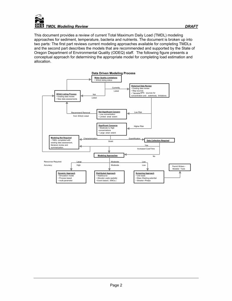
This document provides a review of current Total Maximum Daily Load (TMDL) modeling approaches for sediment, temperature, bacteria and nutrients. The document is broken up into two parts: The first part reviews current modeling approaches available for completing TMDLs and the second part describes the models that are recommended and supported by the State of Oregon Department of Environmental Quality (ODEQ) staff. The following figure presents a conceptual approach for determining the appropriate model for completing load estimation and allocation.

Historical Data Review • Existing data review• Map sources• TabulatieNPS sources forconcentration and waterbody limitations

Water Quality Limitations • 303(d) listing status

Currently

Listed

Not

Listed

303(d) Listing Process • Existing data review• New data assessments

Low RiskNot Significant Concern • Low concentration• Limited areal extent

Recommend Removal

from 303(d) Listed

Significant Concerns • Moderate to Highconcentrations• Large areal extent

Higher Risk

Modeling Not Required • TMDL completed withexisting data assessment,literature review andsummarization.

GoalsCharacterization Quantification

Modeling Approaches

Distributed Approach • HeatSource• Allocate Loads spatially• Event based ( EMCs )

Dynamic Approach • Simulation model• Process based• multi-parameter

Data Collection Required

Yes

Increased Cost/Time

No

Screening Approach • Unit loads• Mass Wasting potential• Streeter -Phelps

Resources Required: Large Moderate Low

Accuracy: High Moderate Low

Data Driven Modeling Process

Permit Writers -Modeler Tools


Part 1 – Review of Nonpoint Source Modeling Methods The current schedule requires that ODEQ complete TMDLs to address all 303(d) listed stream reaches in the state by 2007. With the time constraints of such a schedule, it is necessary for the TMDL team to develop efficient processes for determining TMDLs. One of the purposes of this report is to evaluate methods and determine how to increase efficiencies and effectiveness in completing TMDLs in a short time frame while ensuring scientific credibility. To determine the best approach to completing a TMDL, one should evaluate many criteria for selecting the approach and objectively compare the methods. The following is a list of criteria for determining the approach:

• What is the areal (geographic) extent? • What existing data (water quality, hydrology, GIS) are currently available? • Is additional data needed? What will it cost? • Will the data be appropriate for the modeling tasks? • Are the resources for performing the analysis comparable to resources budgeted for

the tasks? • What levels of precision and accuracy are needed and why? • Are there any additional resources (monetary or personnel) that can be used to

complete the project (external to DEQ)? If so, are the resources cost effective for DEQ. Will the analysis provide necessary rigor?

Nonpoint source (NPS) models are tools for estimating and determining water quality impacts to receiving waterbodies. They are useful for allocating loads, evaluating management practices and understanding the basic mechanisms for the transport (routing) and fate of water quality. Therefore NPS models are often critical tools necessary to complete TMDLs that comply with federal statutes. Nonpoint source models are based on large geographic areas, and estimate parameters across those areas which drain into stream, lakes or estuaries. Common nonpoint source water quality parameters include temperature, sediments, nutrients, biochemical oxygen demand, bacteria, toxics, and pesticides. Sources of these pollutants include: thermal impacts from the loss of riparian vegetation; nitrogen and phosphorus fluxes from fertilizers, septic tank systems, or feedlots; sediment sources from construction and timber harvesting; pesticides from agricultural and urban areas; and heavy metals and toxic chemicals from industrial facilities, landfills and urban runoff. Hydrology is often critical to modeling nonpoint source pollution because water flow and routing are the basic transport mechanisms for most pollutants. Some pollutants, such as sediment and total phosphorus are transported primarily by overland flow, whereas nitrogen, soluble phosphorus and pesticides are transported in the saturated soil zone or, in some instances, groundwater. Therefore it is important that hydrology be evaluated in most nonpoint source evaluations.

Figure 1 presents a systematic approach to evaluating NPS models in Oregon for the TMDL process. This approach coordinates data exchange between various modeling approaches and reduces costs.


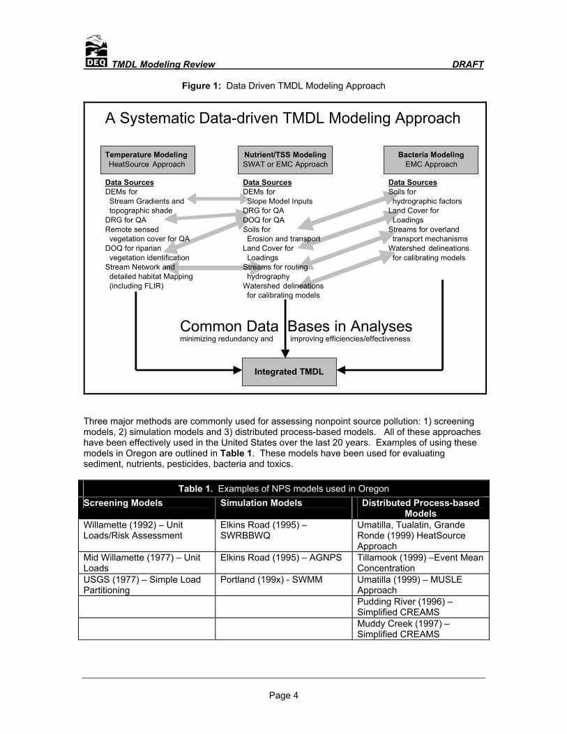
Figure 1: Data Driven TMDL Modeling Approach

Temperature ModelingHeatSource Approach

Nutrient/TSS ModelingSWAT or EMC Approach

Bacteria ModelingEMC Approach

Data Sources DEMs for Slope Model InputsDRG for QADOQ for QASoils for Erosion and transportLand Cover for

LoadingsStreams for routing hydrographyWatershed delineations for calibrating models

Data Sources Soils for hydrographic factorsLand Cover for LoadingsStreams for overland transport mechanismsWatershed delineations for calibrating models

Data Sources DEMs for Stream Gradients and topographic shadeDRG for QARemote sensed vegetation cover for QADOQ for riparian vegetation identificationStream Network and detailed habitat Mapping (including FLIR)

Common Data Bases in Analysesminimizing redundancy and improving efficiencies/effectiveness

A Systematic Data-driven TMDL Modeling Approach

Integrated TMDL

Three major methods are commonly used for assessing nonpoint source pollution: 1) screening models, 2) simulation models and 3) distributed process-based models. All of these approaches have been effectively used in the United States over the last 20 years. Examples of using these models in Oregon are outlined in Table 1. These models have been used for evaluating sediment, nutrients, pesticides, bacteria and toxics.

Table 1. Examples of NPS models used in Oregon Screening Models Simulation Models Distributed Process-based

Models Willamette (1992) – Unit Loads/Risk Assessment

Elkins Road (1995) – SWRBBWQ

Umatilla, Tualatin, Grande Ronde (1999) HeatSource Approach

Mid Willamette (1977) – Unit Loads

Elkins Road (1995) – AGNPS Tillamook (1999) –Event Mean Concentration

USGS (1977) – Simple Load Partitioning

Portland (199x) - SWMM Umatilla (1999) – MUSLE Approach

Pudding River (1996) – Simplified CREAMS

Muddy Creek (1997) – Simplified CREAMS


Screening Models There are several screening tools that can assist in evaluating pesticides, nutrients and bacteria impacts. Unlike detailed process-based simulation models, screening models will not specify exact concentrations but yield rankings and risk potentials. Screening models are simple in nature and rely on very general data. Examples of screening models include a unit load approach, P-Route (for point sources), Oregon Water Quality Decision Aid and other approaches (discussed in the next section). In some cases screening models have been used in conjunction with other models such as process-based simulation models for evaluating water quality impacts (Maidment, 1993; Tian, 1994). Screening models have been used commonly since the 1960’s. The screening model allows prioritization over large geographic areas and the process-based model can be used to evaluate specific factors in areas of high risk. The detailed modeling results are nested hierarchically in a basin based on existing data. The nesting methodology (along with sample statistics) can save major costs and quantify errors. The cost savings are due to reduced labor in data collection, data processing, laboratory analysis and interpretation. Simulation Models There are numerous process-based simulation models that could be easily applied in Oregon to evaluate sediment, nutrient and pesticide contributions to surface water. The most common models include HSPF, CREAMS, ANSWERS, SWMM, SWRRB, SWAT, EPIC and GLEAMS, PRZM, PATRIOT, RZWQM, PESTAN, and LEACHM (most of these models are available at no charge from the EPA Center for Exposure Analysis and Modeling [CEAM] in Athens, GA (Ravi and Johnson, 1994; Knisel, et al. 1991). The major advantage of these models is that they include specific routing and transport mechanisms and can be calibrated to measured concentrations. Table 1 presents the most common nonpoint source models. These models predict concentrations in various components (i.e. soil layers/depths, organic matter, soluble) over time given specific application rates. The differences between these models include plant uptake, different soil inputs, and the number of pesticides that can be simulated. The major disadvantage of process-based models is that they are typically lumped sum parameter models with no detailed spatial components and are typically time consuming to calibrate because many additional parameters have to be included in the model to account for spatial variability. This type of model was very commonly used in the 1970’s and 1980s. The standard water quality simulation models require detailed data and are typically applied at the field scale. Homogeneous areas are usually determined in a GIS, and are often called hydrologic response units (HRU). This approach is similar to hydrologic/water quality models such as SWMM, or HSPF (Donigian and Huber, 1991). Distributed Process-based Models Distributed process-based modeling approaches have become very prevalent in the literature in recent years. Researchers throughout the United States have used a combination of geographic and water quality modeling methods for evaluating quality patterns/impacts to groundwater and surface water (eg. Burkart and James, 1999; Arnold et al, 1998; Burkart et al., 1998; Mizgalewicz, and Maidment, 1996; Battaglin and Goolsby, 1995). Geographic Information Systems (GIS) have been used to assist in this process. GIS is often used to estimate flow in ungaged watersheds (Maidment, 1996) and identify the causal factors associated with the modeling tasks. Instead of summarizing/characterizing the landscape with artificial parameters, as in a standard simulation model, the distributed modeling approach allows site specific data to be incorporated into the model. With the advent of computational capabilities (faster computers) and new software (GIS, remote sensing, etc), distributed process-based models have become an effective and efficient solution for complex water quality modeling.


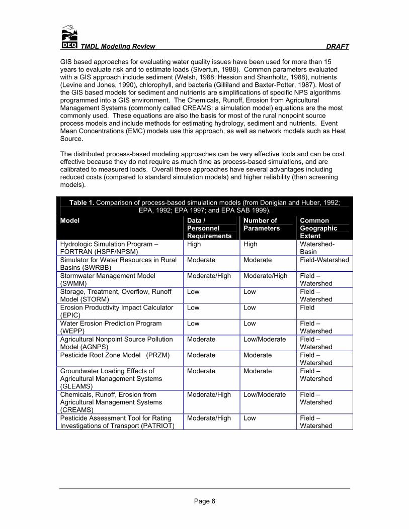
GIS based approaches for evaluating water quality issues have been used for more than 15 years to evaluate risk and to estimate loads (Sivertun, 1988). Common parameters evaluated with a GIS approach include sediment (Welsh, 1988; Hession and Shanholtz, 1988), nutrients (Levine and Jones, 1990), chlorophyll, and bacteria (Gilliland and Baxter-Potter, 1987). Most of the GIS based models for sediment and nutrients are simplifications of specific NPS algorithms programmed into a GIS environment. The Chemicals, Runoff, Erosion from Agricultural Management Systems (commonly called CREAMS: a simulation model) equations are the most commonly used. These equations are also the basis for most of the rural nonpoint source process models and include methods for estimating hydrology, sediment and nutrients. Event Mean Concentrations (EMC) models use this approach, as well as network models such as Heat Source. The distributed process-based modeling approaches can be very effective tools and can be cost effective because they do not require as much time as process-based simulations, and are calibrated to measured loads. Overall these approaches have several advantages including reduced costs (compared to standard simulation models) and higher reliability (than screening models).

Table 1. Comparison of process-based simulation models (from Donigian and Huber, 1992; EPA, 1992; EPA 1997; and EPA SAB 1999).

Model Data / Personnel Requirements

Number of Parameters

Common Geographic Extent

Hydrologic Simulation Program – FORTRAN (HSPF/NPSM)

High High Watershed- Basin

Simulator for Water Resources in Rural Basins (SWRBB)

Moderate Moderate Field-Watershed

Stormwater Management Model (SWMM)

Moderate/High Moderate/High Field – Watershed

Storage, Treatment, Overflow, Runoff Model (STORM)

Low Low Field – Watershed

Erosion Productivity Impact Calculator (EPIC)

Low Low Field

Water Erosion Prediction Program (WEPP)

Low Low Field – Watershed

Agricultural Nonpoint Source Pollution Model (AGNPS)

Moderate Low/Moderate Field – Watershed

Pesticide Root Zone Model (PRZM) Moderate Moderate Field – Watershed

Groundwater Loading Effects of Agricultural Management Systems (GLEAMS)

Moderate Moderate Field – Watershed

Chemicals, Runoff, Erosion from Agricultural Management Systems (CREAMS)

Moderate/High Low/Moderate Field – Watershed

Pesticide Assessment Tool for Rating Investigations of Transport (PATRIOT)

Moderate/High Low Field – Watershed


Further discussion of various models follows: Temperature Models Brown’s equation Browns equation is a physical based heat flux equation. Jobson and Keefer Jobson and Keefer developed a methodology to predict heat transfer on the Chattahoochee River using finite difference methods (hydro-pulsated system). Beschta and Weatherred Beschta and Weatherred contributed quantitative descriptions of heat energy flux components, particularly convection, conduction, and evaporation. SSTEMP SSTEMP used daily average temperature and estimated daily maximum temperature from an empirical simplification that correlates maximum air and water temperature. MNSTREM MNSTREM (Sinokrot and Stefan) developed a numerical model based on finite difference solution to the unsteady heat advection / dispersion equation in predicting hourly water temperatures. HSPF Chen used a combination of the Hydrologic Simulation Package Fortran (HSPF) and an energy balance methodology to simulate stream temperatures for various hypothetical riparian restoration strategies Heat Source Heat Source uses multiple data sources such as FLIR data, instream hourly temperature data, 1:5000 scale stream and riparian vegetation data, GIS-sampled data, and field-measured hydrology data to accurately predict stream temperature at a 100-foot distances. Heat Source is used to model stream networks as well as point source discharges for the development of TMDL Loading Capacities and Waste Load Allocations. Heat Source is a distributed process-based modeling approach. Sediment and Nutrient Models Unit Load Models Nutrient screening models have been used for many years for evaluating regional impacts (see Jettyjohn et al., 1991). The most common screening model is the unit load approach. This involves associating land use data and areal coverage to estimated average annual loading rates to surface or groundwater (Novonty and Chester, 1981). The only data set usually required is land cover (areal extents). These models typically are low reliability because the model results cannot be compared to measured values. Oregon Water Quality Decision Aid The Oregon Water Quality Decision Aid (OWQDA) is a screening tool that allows the evaluation of the likelihood that specific chemicals, when applied to soil, will move through the soil and contaminate groundwater. This program has a user-friendly interface with a complete Oregon soils and pesticides database. Soils sensitivity is evaluated based on permeability, soil depth, slope, organic matter and clay content. Pesticide movement is rated based on the chemical half-life and mobility. Although the ranking/rating methods identified in the OWQDA software is set up


for individual soils and pesticides, its methods could be easily incorporated into a GIS to create a hybrid approach. Soils and land use (a surrogate for pesticide applications) can be overlaid in a GIS and a spreadsheet can be used for ranking. CMLS CMLS is another screening type model that can serve as a management tool and a decision aid for the application of organic chemicals (Nofziger and Hornsby, 1986). It can estimate the movement of chemicals in soils and response to downward movement of water. Li et al. (1990) have also presented a screening model for evaluation of pesticides using data from regression models derived from field data. P-Route P-ROUTE is a simple routing model that estimates point and non-point source pollutant concentrations on a reach by reach flow basis using 7Q10 or mean flow. Event Mean Concentrations Event Mean Concentration (EMC) typically uses a unit load type approach where a concentration is associated with a specific land cover and the water volume from a storm event. The water volume is usually estimated with the SCS, or rational methods. Kinematic wave theory (Chow et al., 1988) can be used to estimate time of concentration and related to first order decay rates. This approach is well suited to being completely distributed and is calibrated to measured data. HSPF HSPF is a simulation model developed by EPA that predicts water quality for numerous constituents including conservative and non-conservative parameters. The model uses a wash-off routine for estimating pollutant loads and simulating hydrology. HSPF requires extensive hydrologic data including continuous precipitation, evaporation, and temperature. This model has been incorporated into EPA Better Assessment Science Integrating Source and Nonpoint Sources (BASINS). SWAT SWAT is a process-based model that uses the CREAMS algorithms combined with the erosion (MUSLE) and groundwater/subsurface (GLEAMS) equations for estimating hydrology and water quality (primarily sediment, nutrients and pesticides). The SWAT model (modified version of the SWRBB model; Arnold, et al. 1993; Arnold and Williams, 1987) has incorporated an ArcView interface for assisting in determining information for watersheds. The model requires the studied watershed to be partitioned into homogeneous response units (HRUs), (i.e. similar in soils, slope and land use). The advantage of this approach over the standard SWRRB or SWAT model is that the GIS interface allows users more control of the spatial components of the model and assists with setting up calibration parameters. SWAT’s newest improvements allow complete distribution (via a GIS interface) within the model. AGNPS AGNPS is a spatially distributed nonpoint source model, which uses a grid cell based modeling approach (Young, et al., 1989). AGNPS has been widely used for estimating sediment and nutrients. The model has an interface to GIS (the GRASS System). Pesticides can be applied and routed in this model (beta release). The newest version of this model (AGNPS98) will also include tools for characterizing reaches, in-stream sediment processes (CONCEPTS), temperature (SNTEMP), and salmonid responses to sediment (SIDO). SEAMS Soil, Environmental and Agricultural Management System (SEAMS) is an ArcView interface to the CMLS model that was developed for watersheds in Florida (Hoogeweg and Hornsby, 1998). This tool consists of several modules for evaluating pesticide risks. Currently the model only has data files for Florida. The SWMM model has a set of tools for ArcView (SWMMTools) for


generating input files. Other models with GIS interfaces include ModFlow, WASP (Chen, 1995; Benaman et al., 1996) and other specified models. Bacteria Models HSPF HSPF (discussed above) also can be used to estimate bacteria concentration in a stream. An advantage of HSPF for bacteria (biological) modeling is that fine time steps (minutes, hours, etc) can be modeled if data is available. This modeling approach usually requires significant time and resources to complete. SWAT SWAT has new bacteria processes incorporated and ODEQ is going to do beta evaluations and tests of these models for the USDA Agricultural Research Service. EMC Event Mean Concentration approaches have been used extensively to model various constituents since the 1980’s (Huber, 1993). Several bacteria TMDLs have been determined by Oregon DEQ using the EMC approach including Tillamook, Tualatin, Umatilla and the Nestucca River. Other examples of EMC modeling approaches include: Quenzer and Maidment, 1998; Melancon, et al 1999; EPA, 1983; and EPA 1992. Simple Point Source/Decay Models There are several models which have simple first order decay capabilities for evaluating bacteria in-stream. Loads are typically requires as inputs into these models. Examples include QUAL2EU and P-Route. Additional Models Useful for Determining Loading Capacities In addition to nonpoint source load allocation modeling, modeling is often needed to determine receiving water loading capacities. Loading capacity modeling is generally needed in complex situations, such as when the standard is being violated is different than the pollutant being allocated or when a parameter undergoes phase changes from a less toxic to more toxic form. Many of the models for determining loading capacities provide detailed information on the fate, transformation and transport of organic chemicals. Examples of models used in the State of Oregon to determine loading capacities include QUAL2E, CE-QUAL-W2, WASP, modified Streeter-Phelps DO models, periphyton models, and toxicity models, as follows: QUAL2E The Enhanced Stream Water Quality Model (QUAL2E) is a user-friendly one-dimensional, hydraulically steady-state stream model that has been used extensively throughout Oregon and North America (Brown and Barnwell 1987). 15 constituents may be modeled including temperature, dissolved oxygen, BOD, phytoplankton, nitrogen, phosphorus, bacteria, and arbitrary conservative and non-conservative constituents. QUAL2E is generally operated as a steady-state model in order to calculate daily average concentrations, but does have limited dynamic capabilities. For example it can calculate diel dissolved oxygen dynamics due to algal growth and respiration. An enhancement, QUAL2E-UNCAS, allows uncertainty analyses including sensitivity analyses, 1st order error analyses, and monte carlo simulations. QUAL2E has been used most extensively to determine point source load allocations for BOD, ammonia, and nutrients necessary to meet dissolved oxygen standards. QUAL2E is supported by the U.S. EPA Center for Exposure Assessment Modeling. Example Applications: Willamette River, Pudding River, South Yamhill River


CE-QUAL-W2 CE-QUAL-W2 is a two-dimensional, laterally averaged, hydrodynamic and water quality model. It is best suited for relatively long and narrow rivers, lakes, reservoirs and estuaries exhibiting longitudinal and vertical water quality gradients (Cole and Buchak 1994, Cole and Wells 2000). Considerable flexibility is provided for modeling hydraulic structures such as culverts, spillways, weirs, and selective withdrawal structures. 34 water quality constituents may be modeled including temperature, dissolved oxygen, labile and refractory dissolved and particulate organic matter, dissolved and suspended solids, bacteria, phosphorus, nitrogen, phytoplankton, inorganic carbon, alkalinity, and pH. A recent version of the model includes a shade routine that allows shade and temperature to modeled in a method similar to the DEQ temperature model Heat Source. As a dynamic model, CE-QUAL-W2 can calculate the full diel cycle and, therefore, calculate daily maximum temperature, daily minimum DO, and daily maximum and minimum pH. This allows direct comparisons of model calculations to water quality standards. Simulations can also be performed for long time periods and non-steady state flow conditions. Therefore, critical salmonid spawning periods may be evaluated in addition to critical summer low flow periods. CE-QUAL-W2 is supported by the U.S. Army Corps of Engineers Waterways Experiment Station. Many recent enhancements have been made to the model by Dr. Scott Wells at Portland State University under contract with the Corps. Example Applications: Tualatin River, Bull Run, Clackamas River, Snake River (including Brownlee Reservoir). WASP The Water Quality Analysis Simulation Program (WASP) is a dynamic modeling system that can be used to analyze a variety of water quality problems in streams, lakes, reservoirs and estuaries. Based on the flexible compartment modeling approach, WASP can be applied in one, two or three dimensions and is designed to permit easy substitution of user- written routines into program structure. Problems studied using WASP include biochemical oxygen demand and dissolved oxygen dynamics, nutrients and eutrophication, bacterial contamination, and organic chemical and heavy metal contamination. WASP consists of two models: TOXI5 calculates dissolved and sorbed toxic pollutant concentrations in the bed and overlying waters; EUTRO5 calculates DO and phytoplankton dynamics affected by nutrients and organic material. WASP is applied by DEQ in specialized applications such as estuaries where three-dimensional modeling is necessary or where specialized kinetic sub-routines are needed to model complex pollutants. WASP does not model hydrodynamics, so a separate hydrodynamics model, such as the companion model DYNHYD, may be needed if hydrodynamics are complex. WASP is supported by the U.S. EPA Center for Exposure Assessment Modeling. Example Applications: South Fork Coquille River Streeter-Phelps DO models DEQ has developed simplified dissolved oxygen models for streams that utilize modified Streeter-Phelps equations. These calculate dissolved oxygen concentrations downstream from point sources for steady-state flow conditions. The models are in the form of executable DOS routines and Microsoft Excel routines and provide user-friendly alternatives to modeling with QUAL2E. The models are supported by the DEQ Water Quality Division Watershed Management Section. Example Applications: Water quality-based NPDES permits, Wildhorse Creek TMDL Periphyton Control Model The Periphyton Control Model (PCM) is a stream periphyton model developed by DEQ to evaluate the sensitivity of diel DO and pH fluctuations to solar radiation, temperature, nitrogen, phosphorus, depth and turbidity (ODEQ 2000). The model is calibrated on critical condition diel DO and pH data, such as from Hydrolab datasondes, collected at several locations along a stream. When coupled with a temperature model, such as Heat Source, PCM can indicate


whether shade improvements necessary to meet temperature standards will also result in pH and DO standards being met, or whether nutrient reductions are also necessary. PCM is supported by the DEQ Water Quality Division Watershed Management Section. Example Application: Grande Ronde River SMPTOX3 The Simplified Method Program - Variable Complexity Stream Toxics Model (SMPTOX3) is a user-friendly one-dimensional steady-state model for developing wasteload allocations for toxic pollutants (Tetra Tech and Limno-Tech 1993). It models dissolved and particulate (sorbed) toxic pollutant phases in both the water column and bedded sediment, water column suspended solids, and bed interactions. Processes modeled include equilibrium partitioning of toxic pollutant between particulate and dissolved phases, settling and resuspension of solids and associated toxic pollutant, sediment-water diffusion of dissolved phase toxic pollutant, and toxic pollutant decay, photolysis, and volatilization. SYMPTOX3 is supported by the U.S. EPA Center for Exposure Assessment Modeling. Example Application: Willamette River Part 2 – Recommended and Supported Nonpoint Source and Temperature TMDL models Since it is financially impossible for ODEQ to have in-house expertise on all of the NPS models, ODEQ staff (modelers, GIS, database, etc) have attempted to develop specific expertise in several models. Several issues were evaluated in choosing the appropriate models:

• Is the model applicable at various scales? • Can the model easily deal with dynamic simulations/data? • Is the model geographically variable enough to represent diverse landscapes present

in Oregon? • Is the approach based on sound scientific principles? • Can the modeling approach be cost effectively employed?

Increasing the technical expertise with a few specific models increases the speed at which the modeling can be completed, allows stronger understanding of the underlying processes impacting water quality, and reduces costs. This cost effectiveness is extremely important because ODEQ staff is charged with producing TMDLs at a very rapid pace with limited resources. The following graph presents data from EPA (1996) on the cost of preparing TMDLs. The graph demonstrates that as the areal extent of the watershed increases, the cost only nominally increases (indicating that large area TMDLs are much more cost effective). Based on previously completed TMDLs by ODEQ staff, these costs can actually be significantly lowered by clearly defining the modeling process a priori in order to focus data collection and analytical efforts.


Figure 2. Costs for completing TMDLs (EPA, 1996).

TMDL Modeling Costs

$0

$50,000

$100,000

$150,000

$200,000

$250,000

$300,000

$350,000

0 100 200 300 400 500 600 700Water Size (Sq. Miles)

Cos

ts

- 2 FTE

- 3 FTE

- 1 FTE

- 3 FTE

- 5 FTE

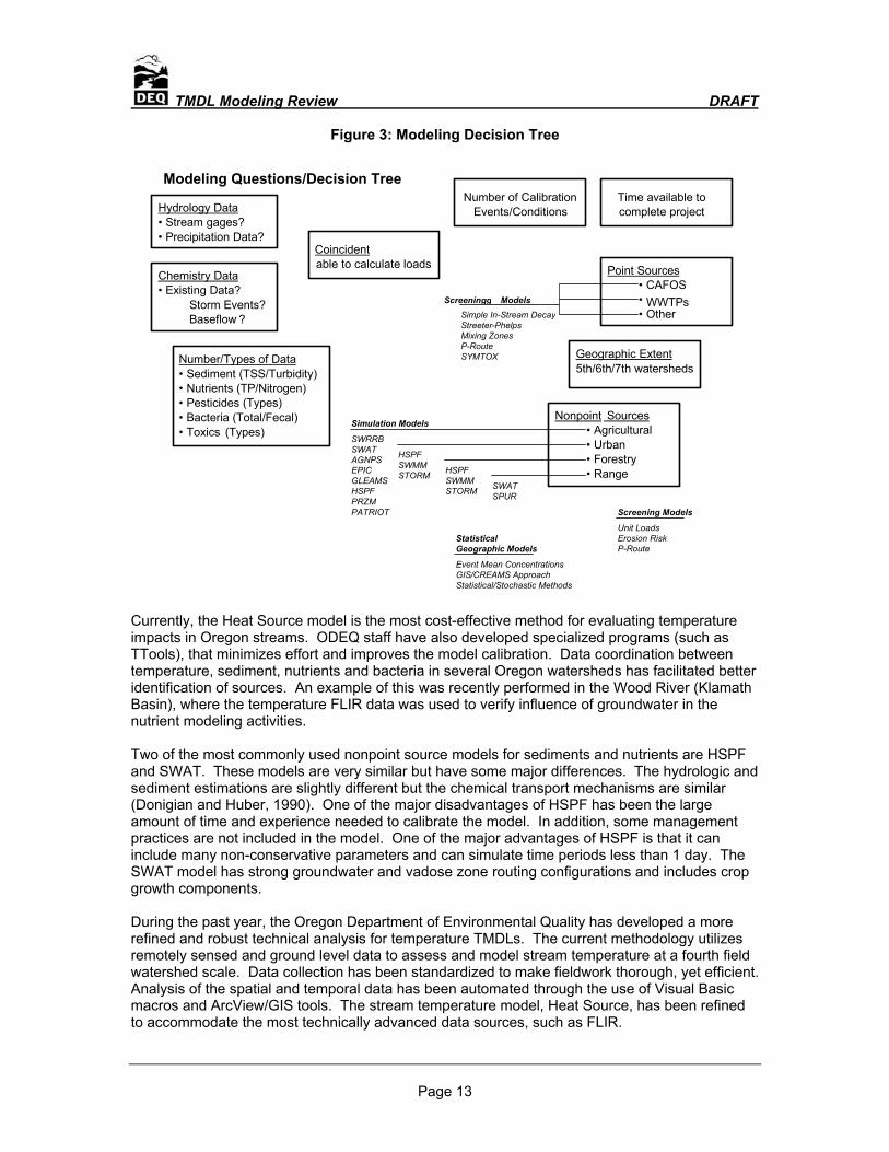
The various modeling approaches require different time commitments to obtain data, prepare inputs, calibrate models, run scenarios and prepare results. For example, using HSPF for a 250 to 350 square miles watershed would require 5 FTE for a minimum of 1 year (EPA, 1996; EPA Midwest Agricultural Subsurface Transport and Effects Research and USDA Midwest Effects Program), whereas using a model such as SWAT (based on ODEQ current activities) requires 2 FTE for 2 to 3 months. In comparison, using a simplified EMC approach would require only 1 FTE for less than 1 month. The more resource demanding approaches can improve modeling accuracy and precision, which may allow smaller margins of safety, higher load allocations, greater confidence that standards will be met, and potentially greater acceptance by local stakeholders. The more resource demanding approaches also may also allow multiple parameters to be addressed using a single model. Selection of the most cost-effective modeling approach depends upon available resources and the potential impact that the modeling may have on load allocations. Figure 3 presents some of the major decisions that are evaluated when determining the appropriate sediment/nutrient model.


Figure 3: Modeling Decision Tree

Modeling Questions/Decision Tree

Chemistry Data • Existing Data?

Storm Events?Baseflow ?

Hydrology Data • Stream gages?• Precipitation Data?

Coincident able to calculate loads

Number/Types of Data • Sediment (TSS/Turbidity)• Nutrients (TP/Nitrogen)• Pesticides (Types)• Bacteria (Total/Fecal)• Toxics (Types)

Number of CalibrationEvents/Conditions

Time available tocomplete project

Point Sources • CAFOS• WWTPs• Other

Nonpoint Sources • Agricultural• Urban• Forestry• Range

Simple In-Stream DecayStreeter-PhelpsMixing ZonesP-RouteSYMTOX

Screeningg Models

Simulation Models

SWRRBSWATAGNPSEPICGLEAMSHSPFPRZMPATRIOT

HSPFSWMMSTORM HSPF

SWMMSTORM SWAT

SPUR

Unit LoadsErosion RiskP-Route

Screening Models

Event Mean ConcentrationsGIS/CREAMS ApproachStatistical/Stochastic Methods

StatisticalGeographic Models

Geographic Extent 5th/6th/7th watersheds

Currently, the Heat Source model is the most cost-effective method for evaluating temperature impacts in Oregon streams. ODEQ staff have also developed specialized programs (such as TTools), that minimizes effort and improves the model calibration. Data coordination between temperature, sediment, nutrients and bacteria in several Oregon watersheds has facilitated better identification of sources. An example of this was recently performed in the Wood River (Klamath Basin), where the temperature FLIR data was used to verify influence of groundwater in the nutrient modeling activities. Two of the most commonly used nonpoint source models for sediments and nutrients are HSPF and SWAT. These models are very similar but have some major differences. The hydrologic and sediment estimations are slightly different but the chemical transport mechanisms are similar (Donigian and Huber, 1990). One of the major disadvantages of HSPF has been the large amount of time and experience needed to calibrate the model. In addition, some management practices are not included in the model. One of the major advantages of HSPF is that it can include many non-conservative parameters and can simulate time periods less than 1 day. The SWAT model has strong groundwater and vadose zone routing configurations and includes crop growth components. During the past year, the Oregon Department of Environmental Quality has developed a more refined and robust technical analysis for temperature TMDLs. The current methodology utilizes remotely sensed and ground level data to assess and model stream temperature at a fourth field watershed scale. Data collection has been standardized to make fieldwork thorough, yet efficient. Analysis of the spatial and temporal data has been automated through the use of Visual Basic macros and ArcView/GIS tools. The stream temperature model, Heat Source, has been refined to accommodate the most technically advanced data sources, such as FLIR.


Below are brief descriptions of the innovative data sources and applications which have become part of the Oregon DEQ’s temperature TMDL technical analysis within the past year. Including using Forward Looking Infrared Radiometry (FLIR), Aerial Photograph Mapping and specialized GIS tools:

• A high-resolution infrared camera is mounted to a helicopter and records a spatially continuous longitudinal temperature profile of the stream. This data is used to assess the current conditions, identify significant groundwater sources, examine point source effects, and to calibrate the temperature model.

• High-resolution (one meter pixel) orthorectified aerial photographs are used to digitize the streams and riparian vegetation at a 1:5000 or smaller scale. Ground level riparian data is collected and used to assign species composition, stand height, and canopy density values to the mapped riparian vegetation.

• ODEQ staff has written an ArcView extension that automatically samples the following parameters every 100 longitudinal feet along a stream improving cost effectiveness and minimizing data input errors: stream aspect, stream elevation and gradient, topographic shading (West, South, and East), channel width, and riparian vegetation

Based on information in the model review, available time, resources, data, and other issues, the following were identified as primary models for completing Oregon’s TMDLS: Heat Source for temperature, SWAT for sediments/nutrients/pesticides and possibly bacteria, and the EMC approach for bacteria and some nutrient issues. The following figure presents some of the issues the users must evaluate before choosing the appropriate model for a sediment/nutrient TMDL. This type of process has been completed by ODEQ staff for numerous TMDLs that have been completed and approved (or are pending) at EPA including the following subbasins/watersheds: Umatilla, Grande Ronde, Tillamook, Tualatin. In addition, work is currently underway for completing the Nestucca, Wood, Sprague, Williamson, Wallowa, and Hood subbasins in 2000 and early 2001. Heat Source Advantages

• Distributed Process-based model • Designed to utilize available spatial data sets • Easy to set up and calibrate model • Directly determines Load Allocations and Surrogate Measures • Effective for Agricultural, Range, Forest and Urban areas • Management practices/BMPs can be easily incorporated

SWAT Advantages

• Distributed Process-based model • Simulates hydrology from climate • ARS model with EPA support (BASINS) • Effective for Agricultural, Range, Forest and Urban areas • Management practices/BMPs can be easily incorporated

EMC Advantages

• Distributed Process-based model • Easy to set up and calibrate model • Management practices/BMPs can be easily incorporated


Heat Source Temperature Model Heat Source uses spatially distributed data and process based equations for simulating stream temperature. Heat Source uses a finite difference method to solve the non-uniform heat energy transfer equation. The model also considers advection, dispersion, and heat energy flux. The Heat Source methodology is designed to utilize spatial data set and utilizes GIS tools to efficiently and accurately sample these data sets. The major Heat Source modeling steps are:

1. Identify Data Needs and Obtain/Organize Data 2. Determine the Indicator Streams/Rivers to Be Modeled/Analyzed 3. Digitize Indicator Steam/River 4. Use Ttools to create Spatial Data 5. Input Data into Model 6. Calibrate model 7. Develop and Run scenarios

SWAT Sediment/Nutrient/Pesticide Model SWATs primary objective is to predict the effect of management decisions on water, sediment, nutrient and pesticide yields with reasonable accuracy on large, ungaged river basins. The model simulates hydrology (including surface runoff, return flow, percolation, ET, transmission losses, pond & reservoir storage, crop growth & irrigation, groundwater flow, reach routing) and nutrient (nitrogen and phosphorus) & pesticides loading. The model functions on a daily time step and can account for differences in soils, land use, crops, topography, weather, etc. Basins of several thousand square miles can be studied and the model uses measured data & point sources. The major SWAT modeling steps are (see appendix for more detailed sprocess):

1. Prepare Climate data for model input 2. Prepare hydrology and water chemistry data for calibration 3. Prepare GIS data base (Soils, land use, Homogenous Response Units, etc) 4. Set up model/Initial runs 5. Incorporate other processes (hydrology storage, withdrawals ,etc) 6. Calibrate Hydrology 7. Calibrate Sediment 8. Calibrate Phosphorus 9. Calibrate Bacteria 10. Calibrate Nitrogen 11. Calibrate Pesticides 12. Run Scenarios

EMC Bacteria/Nutrient Model The primary objective of an EMC approach is to predict the loads from various land management practices on ungaged and gaged river basins. The EMC approach estimates runoff volumes and correspondingly pollutant loads.


This simple modeling approach typically functions on an event or in some cases a daily time step. Various landscape factors are included in the analyses. ODEQ EMC methods have used the SCS method for estimating flow volume, rational formula to estimate flow rates, kinematic wave for estimating time of concentration, and first order decay rates for biological die-off. The major EMC modeling steps are:

1. Prepare precipitation data for model input 2. Prepare hydrology and water chemistry load data for calibration targets 3. Prepare GIS data base 4. Combine (overlay) GIS data for input into model 5. Calibrate Hydrology (adjust curve numbers/land uses) 6. Calibrate Bacteria/Nutrients 7. Run Scenarios/examine loads by DMAs

References Ambrose, R.B., T.A. Wool, J.P. Connolly, and R.W. Schanz. 1988. WASP4, A Hydrodynamic And Water Quality Model – Model Theory, User’s Manual, And Programmer Guide. U.S. Environmental Protection Agency, Athens, GA. EPA/600/3-87/039. Arnold, J.G., P.M. Allen and G. Bernhardt, 1993. A comprehensive surface-groundwater flow model [SWAT], Journal of Hydrology, 142:47-69. Arnold, J. G.. and J. R. Williams. 1987. Validation of SWRRB - Simulator of Waters in rural basins. J. Water Resources Planning and Management. ASCE 113(2):243-246. Barbash, J.E., G. P Thelin, D.W. Kolpin and R.J. Gilliom, 1999. Distribution of major herbicides in groundwater in the United States, USGS WRIR 98-4245. Battaglin, W.A. and D. Goolsby, 1995. Spatial data in GIS format on agricultural chemical use, land use and cropping practices in the United States, USGS Water Resources Investigation 94-4176, Denver, CO. Benaman, J., N.E. Armstrong and D.R. Maidment, 1996. Modeling of Dissolved Oxygen in the Houston Ship Channel using WASP5 and Geographic Information Systems, CRWR Online Report 96-2. Bernert J.A., J. M. Eilers , B. J. Eilers , E. Blok2, S.G. Daggett , and K.F. Bierly , 1999. Recent wetlands trends (1981/82-1994) in the Willamette Valley, Oregon, USA, Wetlands, 13:3 Bernert, J.A., J.M. Eilers, T.J. Sullivan, K.E. Freemark, and C. Ribic, 1997. A quantitative methods for delineating regions: An example for the Western Corn Belt Plains Ecoregion of the USA. Environmental Management, 21:405-420. Brown, L.C. and T.O. Barnwell. The Enhanced Stream Water Quality Models QUAL2E and QUAL2E-UNCAS: Documentation And User Manual. U.S. Environmental Protection Agency, Athens, GA. EPA/600/3-87/007. Burkart, M.F., P.W. Gassman, D.E. James, K.W. Kolpin, 1998. Regional groundwater Vulnerability to Agrichecmicals, National Soil Tilth Laboratory, Ames, IA.


Burkart, M.R. and James, D.E., 1999. Agricultural-Nitrogen Contributions to Hypoxia in the Gulf of Mexico. Journal of Environmental Quality 28(3):850-859 Burkart, M and D. Kolpin, 1993. Hydrologic and land use and factors associated with herbicides and nitrates in near surface aquifiers, Journal of Environmental Quality, 22:646-656. Burkart, M.R. D.W. Kolpin, R.J Jaquis, and K.J. Cole, 1999, Agrichemicals in Groundwater of the midwestern United States: relation to soils characteristics, Journal of Environmental Quality, 28:1908:1915. Chen, C.L, L.E. Gomez, C.W. Chen, C.M Wu, J.J. Lin and I.L Cheng, 1995. An integrated Watershed Management model with GIS and Windows Application, International Symposium on Water Quality Modeling, Orlando, Florida, pp242-250. Chen, H. and D. Druliner, 1988. Agricultural chemical contamination of ground water in six areas of the High Plains Aquifer, Nebraska, National Water Summary, 1986, Water Supply Paper 2325, Reston Virginia, USGS. Cole, T.M. and E.M. Buchak. 1994. CE-QUAL-W2: A Two-Dimensional Laterally Averaged, Hydrodynmaic And Water Quality Model, Version 2.0. U.S. Army Corps of Engineers Waterways Experiment Station, Vicksburg, MS Cole, T.M. and S. Wells. 2000. CE-QUAL-W2 Version 3 Workshop, August 21-25, 2000, Portland State University DiGuardo, A. A. Williams, R.J. Mattiessen, P., Brooke, D.N. and D. Calamrai, 1994. Simulation of pesticide runoff at Rosemaund farm using the SoilFug model, Environmental Science and Pollution Research, 1:151-160. Donigian, A.D., Jr., Huber, W.C. and T.O. Barnwell, Jr., "Modeling of Nonpoint Source Water Quality in Urban and Nonurban Areas," Chapter 7 in Nonpoint Pollution and Urban Stormwater Management, V. Novotny, ed., Technomic Publishing Co., Inc., Lancaster, PA, 1995, pp. 293-345. Donigian, A.D. and W.C. Huber, 1991. Models of nonpoint source water quality, EPA, Athens, GA. EPA, 1983. Results of the Nationwide Urban Runoff Program, Volume I – Final Report. EP1.2:N21/8/V.1, Washington, D.C. EPA, 1992. Compendium of Watershed-Scale models for TMDL development, EPA841-R-94002, Washington DC. EPA, 1996. TMDL development Cost Estimates: Case Studies of 14 TMDLs, Washington, DC, EPA-R-96-01. EPA, 1997. Compendium of Tools for Watershed Assessment and TMDL Development, EPA841-B-97-006, Erwin, M.L. and A.J. Tesoriero, 1997 Predicting Groundwater vulnerability to nitrate in the Puget Sound Basin, USGS Fact Sheet, FS-0161-97.


Hession, W.C. and V.O Shanholtz, 1988. A GIS for targeting nonpoint source agricultural pollution, Journal of Soil and Water Conservation, 43:264-266. Hoogeweg, C.G. and A.G. Hornsby, 1998. Soil, Environmental and Agricultural Management System: SEAMS Versions 1.0, University of Florida, SW112. Huber, W.C., 1993, Contaminant Transport in Surface Water, Handbook of Hydrology, edited by D.R. Maidment, McGraw-Hill, Inc., New York. Gilliland, M.W. and W. Baxter-Potter, 1987. A GIS to predict nonpoint source pollution potential, Water Resources, Bulletin, 17:410-420. Knisel, W. G., R. A. Leonard, F. M. Davis, and J. M. Sheridan. 1991. Water balance components in the Georgia Coastal Plain: A GLEAMS model validation and simulation. 46(6):450-456. Levine, D.A. and W.W. Jones, 1990. Modeling phosphorus loading to three Indiana reservoirs: A GIS Approach, Lake and Reservoir Management, 6:81-91. Li, W. D.E. Merrill, and D.A. Haith, 1990. Loading functions for pesticide runoff. Research Journal of the WPCF, 62:16-26. Melancon, P.A., Barrett, M.E. and Maidment, D.R., 1999. A GIS Based Watershed Analysis System for Tillamook Bay, Oregon, CRWR Online Report 99-3. Maidment, D.R. 1993. GIS and hydrology modeling, in Environmental modeling with GIS, edited by Goodchild, M.F., Parks, B.O, and L.T. Steyaert, Oxford university Press. Maidment, D.R., 1996. GIS and Hydrologic Modeling - an Assessment of Progress, Presented at The Third International Conference on GIS and Environmental Modeling, in Santa Fe, New Mexico Maidment, D.R. 19xx. Handbook of Hydrology, editor, John Wiley and Sons. McCuen, 1998. Hydrologic Analysis and Design, Prentise Hall, New York. Mizgalewicz, P.J., and D.R. Maidment, 1996. Modeling Agrichemical Transport in Midwest Rivers using Geographic Information Systems, Center for Research Water Resources, report 96-6:, Austin, TX. Moorman, T.B. and D.B. Jaynes, C.A. Cambardalla, J.L. Hatfield, R.L. Pfeiffer and A.J. Morrow, 1999. Water quality in Walnut creek watershed: herbicides in soils, subsurface drainage and groundwater, 1999. Journal of Environmental Quality, 28:35-45. National Research Conucil, 1993. Groundwater Vulnerability Assessment: Predicting relative contamination potential under conditions of uncertainty, National Academy Press, Washington DC. Newell, A, and J. Bernert, 1996 Scientific and Management Issues in Oregon’s Lake Ecoregions, Northwest Science, 70:1-12. Nofziger D.L. and A.G. Hornsby, 1986. A microcomputer based management tool for chemical movement in soils [CMLS], Applied agricultural Research, 1:50-56.


Novotny, V. and G. Chesters, 1981. Handbook of Nonpoint Source Pollution, VanNostram Reinhold, New York, New York. ODEQ. 2000. Upper Grande Ronde River Sub-Basin Total Maximum Daily Load (TMDL). Oregon Department of Environmental Quality, Portland, OR. Olivera, F., 1996. Spatially Distributed Modeling of Storm Runoff and Non-Point Source Pollution Using Geographic Information Systems, Doctoral Dissertation, University of Texas at Austin - Graduate School, Austin, Texas, http://www.ce.utexas.edu/prof/olivera/disstn/header.htm Olivera F. and D.R. Maidment, 1999. GIS-Based Spatially Distributed Model for Runoff Routing, Water Resources Research Vol. 35 No. 4 pp. 1155-1164, American Geophysical Union, Washington DC. Olivera, F. and D.R. Maidment, 1998. GIS for Hydrologic Data Development for Design of Highway Drainage Facilities, Transportation Research Record # 1625, pp. 131-138, Transportation Research Board, Washington DC. ODEQ, 1999. Report to the Legislative Assembly: groundwater Quality Protection in Oregon, Portland, OR. Pettyjohn, W.A., M. Savoca and D.Self. 1991. Regional assessment of aquifer vulnerability and sensitivity in the conterminous United States, EPA-600/2/91/043, Ada, OK Pipes, W, O., 1982. Bacterial Indicators of Pollution, CRC Press. Quenzer, A.M. and D.R. Maidment, 1998. A GIS Assessment of the Total Loads and Water Quality in the Corpus Christi Bay System, CRWR Online Report 98-1.

Ravi, V. and J. A. Johnson, 1994. PESTAN: Pesticide Analytical Model, version 4.0 Center for Subsurface modeling, Ada, OK.

Rounds, S.A., Wood, T.M., and Lynch, D.D., 1999, Modeling discharge, temperature, and water quality in the Tualatin River, Oregon: U.S. Geological Survey Water-Supply Paper 2465-B, 121 p.

Sivertun, A., L.E. Reinlet and J. Castensson, 1988. A GIS method to aid in nonpoint source critical area analysis, International Journal of Geographic Information Systems, 2:365:378. Tetra Tech, Inc. and Limno-Tech, Inc. 1993. Willamette River Basin Water Quality Study, Component 2: Toxic Chemical Model Application Report. Tetra Tech, Inc., Redmond, WA. TC8983-02. Tesoriero, A/j. and Voss, F.D. 1997. Predicting the probability of elevated nitrate concentrations in the Puget sound basin-implications for aquifer susceptibility and vulnerability, Groundwater, 35:6:1029-1039.

Tian, X., G.J. Sabbagh, G.W. Cuperus, and M. Gregory, 1994. Integrating mathematical model with GIS to evaluate potential of insecticide leaching and runoff, Proceedings GIS/LIS, 759-768. USDA, 1996. Agricultural Chemical Usage: 1995 Fruit Summary, NASS-ERS, usda.mannlib.cornell.edu/data-sets/input/9X172/96172/agch0796.txt. USDA, 1995. Soil Survey Geographic (SSURGO) data base, NRCS, publication 1527.

http://www.ce.utexas.edu/prof/olivera/disstn/header.htm


Welsh, R., M. Madden Remillard, and R.B. Slack, 1988. Remote Sensing and GIS techniques for aquatic resource evaluation, Photogrammetric Engineering and Remote Sensing, 54:177-185. Wood, T.M. and Rounds, S.A., 1998, Using CE-QUAL-W2 to assess the effect of reduced phosphorus loads on chlorophyll-a and dissolved oxygen in the Tualatin River, Oregon, in Proceedings of the First Federal Interagency Hydrologic Modeling Conference, Las Vegas, Nevada, April 19-23, 1998: U.S. Geological Survey, p. 2-149 - 2-156. Wyoming DEQ, 1998 Wyoming Ground Water Vulnerability Assessment Handbook Young, R.A., C.A. Onstad, D.D. Bosch, and W.P. Anderson, 1989. AGNPS: A nonpoint source model for evaluating agricultural watersheds, Journal of Soil and Water Conservation, 44:168-173.


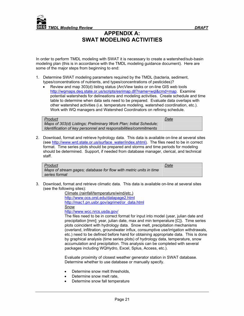
APPENDIX A: SWAT MODELING ACTIVITIES

In order to perform TMDL modeling with SWAT it is necessary to create a watershed/sub-basin modeling plan (this is in accordance with the TMDL modeling guidance document). Here are some of the major steps from beginning to end: 1. Determine SWAT modeling parameters required by the TMDL (bacteria, sediment,

types/concentrations of nutrients, and types/concentrations of pesticides)? • Review and map 303(d) listing status (ArcView tasks or on-line GIS web tools

http://wqmaps.deq.state.or.us/scripts/esrimap.dll?name=wql&cmd=map. Examine potential watersheds for delineations and modeling activities. Create schedule and time table to determine when data sets need to be prepared. Evaluate data overlaps with other watershed activities (i.e. temperature modeling, watershed coordination, etc.). Work with WQ managers and Watershed Coordinators on refining schedule.

Product Date Maps of 303(d) Listings; Preliminary Work Plan; Initial Schedule; Identification of key personnel and responsibilities/commitments

2. Download, format and retrieve hydrology data. This data is available on-line at several sites

(see http://www.wrd.state.or.us/surface_water/index.shtml). The files need to be in correct format. Time series plots should be prepared and storms and time periods for modeling should be determined. Support, if needed from database manager, clerical, and technical staff. Product Date Maps of stream gages; database for flow with metric units in time series format

3. Download, format and retrieve climatic data. This data is available on-line at several sites

(see the following sites): Climate (rainfall/temperature/wind/etc.) http://www.ocs.orst.edu/datapage2.html http://mac1.pn.usbr.gov/agrimet/or_data.html

Snow http://www.wcc.nrcs.usda.gov/ The files need to be in correct format for input into model (year, julian date and precipitation [mm]; year, julian date, max and min temperature [C]). Time series plots coincident with hydrology data. Snow melt, precipitation mechanisms (overland, infiltration, groundwater influx, consumptive use/irrigation withdrawals, etc.) need to be defined before hand for obtaining appropriate data. This is done by graphical analysis (time series plots) of hydrology data, temperature, snow accumulation and precipitation. This analysis can be completed with several packages including WQHydro, Excel, Splus, Access, etc.). Evaluate proximity of closest weather generator station in SWAT database. Determine whether to use database or manually specify.

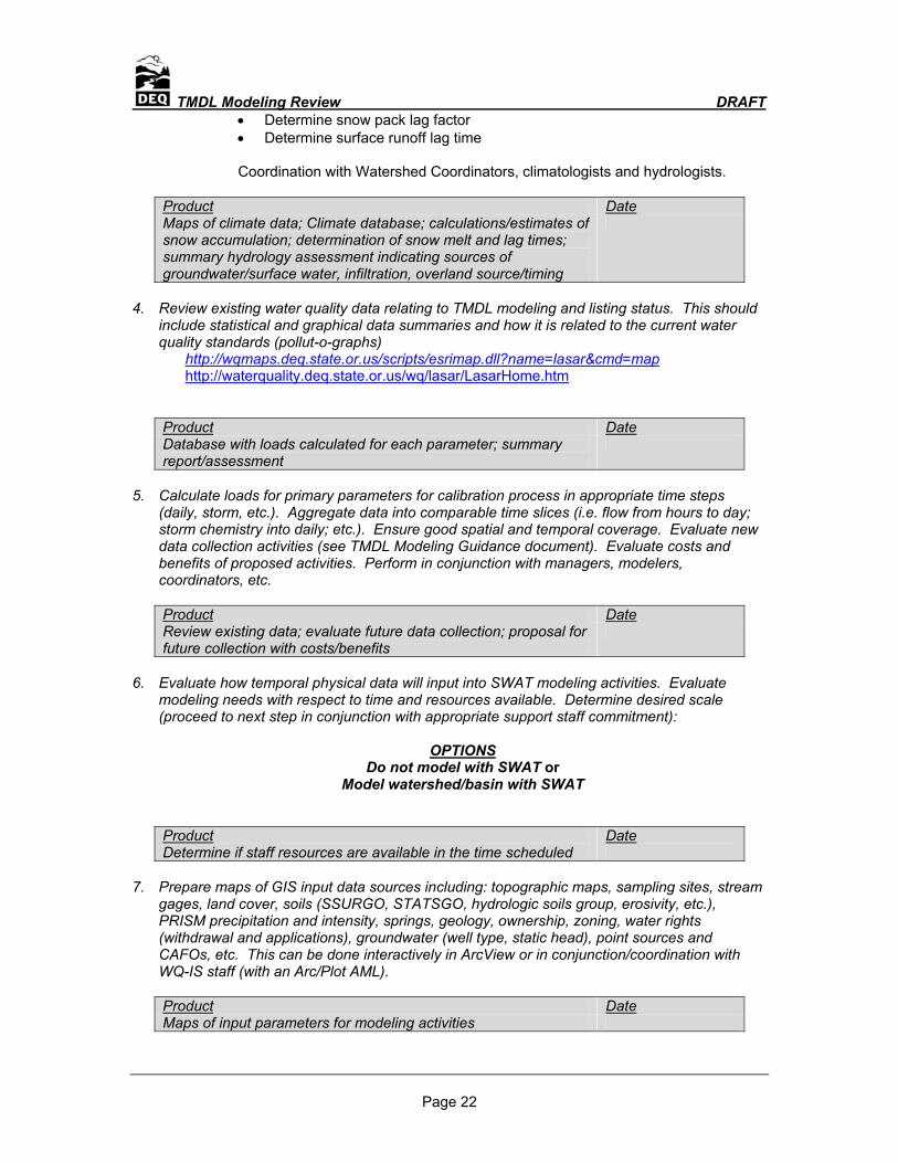
• Determine snow melt thresholds, • Determine snow melt rate, • Determine snow fall temperature

http://wqmaps.deq.state.or.us/scripts/esrimap.dll?name=wql&cmd=map

http://www.wrd.state.or.us/surface_water/index.shtml)

http://www.ocs.orst.edu/datapage2.html

http://mac1.pn.usbr.gov/agrimet/or_data.html

http://www.wcc.nrcs.usda.gov/


• Determine snow pack lag factor • Determine surface runoff lag time

Coordination with Watershed Coordinators, climatologists and hydrologists.

Product Date Maps of climate data; Climate database; calculations/estimates of snow accumulation; determination of snow melt and lag times; summary hydrology assessment indicating sources of groundwater/surface water, infiltration, overland source/timing

4. Review existing water quality data relating to TMDL modeling and listing status. This should

include statistical and graphical data summaries and how it is related to the current water quality standards (pollut-o-graphs)

http://wqmaps.deq.state.or.us/scripts/esrimap.dll?name=lasar&cmd=map http://waterquality.deq.state.or.us/wq/lasar/LasarHome.htm

Product Date Database with loads calculated for each parameter; summary report/assessment

5. Calculate loads for primary parameters for calibration process in appropriate time steps

(daily, storm, etc.). Aggregate data into comparable time slices (i.e. flow from hours to day; storm chemistry into daily; etc.). Ensure good spatial and temporal coverage. Evaluate new data collection activities (see TMDL Modeling Guidance document). Evaluate costs and benefits of proposed activities. Perform in conjunction with managers, modelers, coordinators, etc. Product Date Review existing data; evaluate future data collection; proposal for future collection with costs/benefits

6. Evaluate how temporal physical data will input into SWAT modeling activities. Evaluate

modeling needs with respect to time and resources available. Determine desired scale (proceed to next step in conjunction with appropriate support staff commitment):

OPTIONS

Do not model with SWAT or Model watershed/basin with SWAT

Product Date Determine if staff resources are available in the time scheduled

7. Prepare maps of GIS input data sources including: topographic maps, sampling sites, stream

gages, land cover, soils (SSURGO, STATSGO, hydrologic soils group, erosivity, etc.), PRISM precipitation and intensity, springs, geology, ownership, zoning, water rights (withdrawal and applications), groundwater (well type, static head), point sources and CAFOs, etc. This can be done interactively in ArcView or in conjunction/coordination with WQ-IS staff (with an Arc/Plot AML). Product Date Maps of input parameters for modeling activities

http://wqmaps.deq.state.or.us/scripts/esrimap.dll?name=lasar&cmd=map

http://waterquality.deq.state.or.us/wq/lasar/LasarHome.htm


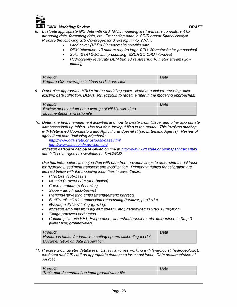
8. Evaluate appropriate GIS data with GIS/TMDL modeling staff and time commitment for preparing data, formatting data, etc. Processing done in GRID and/or Spatial Analyst. Prepare the following GIS Coverages for direct input into SWAT:

• Land cover (MLRA 30 meter; site specific data) • DEM (elevation: 10 meters require large CPU, 30 meter faster processing) • Soils (STATSGO fast processing; SSURGO CPU intensive) • Hydrography (evaluate DEM burned in streams; 10 meter streams [low

points])

Product Date Prepare GIS coverages in Grids and shape files

9. Determine appropriate HRU’s for the modeling tasks. Need to consider reporting units,

existing data collection, DMA’s, etc. (difficult to redefine later in the modeling approaches). Product Date Review maps and create coverage of HRU’s with data documentation and rationale

10. Determine land management activities and how to create crop, tillage, and other appropriate

databases/look up tables. Use this data for input files to the model. This involves meeting with Watershed Coordinators and Agricultural Specialist (i.e. Extension Agents). Review of agricultural data (including irrigation):

http://www.oda.state.or.us/oass/oass.html http://www.nass.usda.gov/census/

Irrigation database can be reviewed on line at http://www.wrd.state.or.us/maps/index.shtml and GIS coverages are available on DEQWQ2. Use this information, in conjunction with data from previous steps to determine model input for hydrology, sediment transport and mobilization. Primary variables for calibration are defined below with the modeling input files in parenthesis. • P factors (sub-basins) • Manning’s overland n (sub-basins) • Curve numbers (sub-basins) • Slope – length (sub-basins) • Planting/Harvesting times (management; harvest) • Fertilizer/Pesticides application rates/timing (fertilizer; pesticide) • Grazing activities/timing (grazing) • Irrigation amounts from aquifer; stream, etc.; determined in Step 3 (Irrigation) • Tillage practices and timing • Consumptive use PET, Evaporation, watershed transfers, etc. determined in Step 3

(water use; groundwater) Product Date Numerous tables for input into setting up and calibrating model. Documentation on data preparation.

11. Prepare groundwater databases. Usually involves working with hydrologist, hydrogeologist,

modelers and GIS staff on appropriate databases for model input. Data documentation of sources. Product Date Table and documentation input groundwater file

http://www.oda.state.or.us/oass/oass.html

http://www.nass.usda.gov/census/

http://www.wrd.state.or.us/maps/index.shtml


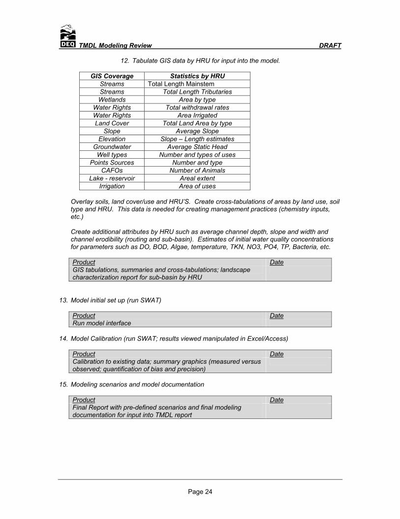
12. Tabulate GIS data by HRU for input into the model.

GIS Coverage Statistics by HRU

Streams Total Length Mainstem Streams Total Length Tributaries Wetlands Area by type

Water Rights Total withdrawal rates Water Rights Area Irrigated Land Cover Total Land Area by type

Slope Average Slope Elevation Slope – Length estimates

Groundwater Average Static Head Well types Number and types of uses

Points Sources Number and type CAFOs Number of Animals

Lake - reservoir Areal extent Irrigation Area of uses

Overlay soils, land cover/use and HRU’S. Create cross-tabulations of areas by land use, soil type and HRU. This data is needed for creating management practices (chemistry inputs, etc.)

Create additional attributes by HRU such as average channel depth, slope and width and channel erodibility (routing and sub-basin). Estimates of initial water quality concentrations for parameters such as DO, BOD, Algae, temperature, TKN, NO3, PO4, TP, Bacteria, etc. Product Date GIS tabulations, summaries and cross-tabulations; landscape characterization report for sub-basin by HRU

13. Model initial set up (run SWAT)

Product Date Run model interface

14. Model Calibration (run SWAT; results viewed manipulated in Excel/Access)

Product Date Calibration to existing data; summary graphics (measured versus observed; quantification of bias and precision)

15. Modeling scenarios and model documentation

Product Date Final Report with pre-defined scenarios and final modeling documentation for input into TMDL report

oregon deq tmdl modeling revie deq tmdl modeling review introduction tmdls specify load allocations...

Documents