order picking problems under weight, fragility, and

June 14, 2016 International Journal of Production Research Warehouse

To appear in the International Journal of Production ResearchVol. 00, No. 00, 00 Month 20XX, 1–22

Order Picking Problems under Weight, Fragility, and Category Constraints

Thomas Chabota∗, Rahma Lahyanib,c, Leandro C. Coelhoa,d, Jacques Renauda

aCIRRELT, Faculté des sciences de l’administration, Université Laval, CanadabCollege of Business, Al Faisal University, Kingdom of Saudi Arabia

cLOGIQ Laboratory, Institut Supérieur de Gestion Industrielle, Sfax, TunisiadCanada Research Chair in Integrated Logistics, Université Laval, Canada

(Received 00 Month 20XX; accepted 00 Month 20XX)

Warehouse order picking activities are among the ones that impact the most the bottom lines of ware-houses. They are known to often account for more than half of the total warehousing costs. New practicesand innovations generate new challenges for managers and open new research avenues. Many practicalconstraints arising in real-life have often been neglected in the scientific literature. We introduce, model,and solve a rich order picking problem under weight, fragility, and category constraints, motivated byour observation of a real-life application arising in the grocery retail industry. This difficult warehousingproblem combines complex picking and routing decisions under the objective of minimizing the distancetraveled. We first provide a full description of the warehouse design which enables us to algebraicallycompute the distances between all pairs of products. We then propose two distinct mathematical modelsto formulate the problem. We develop five heuristic methods, including extensions of the classical largestgap, mid point, S-shape, and combined heuristics. The fifth one is an implementation of the powerfuladaptive large neighborhood search algorithm specifically designed for the problem at hand. We then im-plement a branch-and-cut algorithm and cutting planes to solve the two formulations. The performanceof the proposed solution methods is assessed on a newly generated and realistic test bed containing upto 100 pickups and seven aisles. We compare the bounds provided by the two formulations. Our in-depthanalysis shows which formulation tends to perform better. Extensive computational experiments confirmthe efficiency of the ALNS matheuristic and derive some important insights for managing order pickingin this kind of warehouses.

Keywords: Order picking, warehousing, formulations, exact algorithms, heuristics.

1. Introduction

Order picking represents an important part of warehouse and inventory management activities(Gu et al. 2010). It consists of retrieving goods from specific storage locations to fulfill customersorders. It is considered as the most labor-intensive and costly warehousing activity (de Koster et al.2007; Tompkins et al. 2010), and it may account for up to 55% of all warehouse operating expenses(Chiang et al. 2011). Therefore, warehouse productivity is highly affected by order picking activities(de Koster et al. 2007). Research in this area has rapidly expanded over the past decades. Thesestudies can be categorized into books (Hompel and Schmidt 2006; Ackerman 2013; Manzini 2012),survey papers (Wäscher 2004; de Koster et al. 2007; Henn et al. 2012), and theoretical papersproviding mathematical formulations and exact or approximate solution methods (Bortolini et al.2015; Lu et al. 2016).

Order picking strategies and algorithms have often been studied for classical warehouses (Petersen1997; Petersen and Aase 2004). The role of picker personality in predicting picking performance with

∗Corresponding author. Email: [email protected]


different picking technologies has been studied by de Vries et al. (2015). Recently, some attentionhas been devoted to researches oriented towards more realistic picking contexts (Chackelson et al.2013; Matusiak et al. 2014; Chabot et al. 2015). These cases are either motivated by the complexcharacteristics of real-life warehousing activities, legal regulations, or the introduction of on-lineshopping requiring faster and more customized services.

This paper is motivated by the situation prevailing in the grocery retail industry. In this industry,each company owns one or several distribution centers (DCs) to store its products. Almost all DCsare designed with reserve storage and fast pick areas. In the fast pick area, each stock keeping unit(SKU) is stored in a specific and dedicated location. However, in the reserve storage area, SKUs areplaced at random available locations, but close to the picking and sorting area. Order pickers onlyhave access to the pick area, which is replenished continually by employees from the reserve area.Each order is picked in a sequential way and transported to the sorting area by hand-lift trucks.Each picker deals with a list of products, i.e., a pick-list, to be collected from the storage aisles.

In general, when orders are small compared to the picking vehicle capacity, order batching occurs.Order batching consists of combining orders to reduce the distance traveled by the picker (de Kosteret al. 2007; Petersen 1997; Petersen and Schmenner 1999). Batched orders must later be sorted. Inour case, each individual order may consist of several hundreds of different SKUs, often resultingin thousands of units picked on many pallets.

The sequences followed by the pickers to retrieve all the SKUs of a given order are called routes.A fixed routing plan may perform well for some pick-lists, but poorly for others as decisions aremade sequentially. Thus, the primary and most common objective in manual order-picking systemsis to find the set of picking routes that minimizes the total traveled distance (de Koster and Van derPoort 1998; de Koster et al. 1998; Petersen et al. 2004).

In this paper we develop order picking routes in a warehouse under practical restrictions observedin the grocery retail industry. Each product characteristic considered adds an extra layer of difficultyto the problem. These product-specific properties are described next.

We introduce the order picking problem under weight, fragility, and category constraints (OPP-WFCC). Regarding the weight, as soon as the total weight of all the products transported onthe hand-lift truck exceeds a threshold value, heavy items can no longer be collected, and thepicker is only allowed to pick light SKUs. Thus, another tour is required to pick (some of) theremaining heavy items. This requirement, referred to as weight constraint, has two motivations. Ithelps avoid work accidents and back problems caused by lifting heavy charges to relatively highpositions, and it ensures the vertical and horizontal stability of the pallet. Besides the weight, otherconstraints arise in practice regarding the fragility of the items. A product can support a certainweight without being crushed. Therefore, fragile products must not be placed underneath heavyproducts, i.e., heavy products must be on the bottom of the pallet and light products on the top.We refer to this restriction as fragility constraint and the maximum weight a product can supportis referred to hereinafter as self-capacity. Finally, we consider two types of commodities: food andnon-food products. Non-food products encompass household items. Food products should not becarried under non-food on the pallet in order to avoid contamination. Thus, one has to pick thenon-food products separately or before any food products. This constraint is referred to as categoryconstraint.

Order picking problems dealing with the physical properties of the products have not been widelystudied in the literature, but similar constraints appear in other contexts. Matusiak et al. (2014)refer to these constraints as precedence constraints since they impose that some products must bepicked before some others due to weight restrictions, fragility, shape, size, stackability, and pre-ferred unloading sequence. They propose an heuristic method to solve the joint order batchingand picker routing problem without any specific assumption regarding the layout and without anypre-determined sequencing constraints. Junqueira et al. (2012) introduce the problem of loadingrectangular boxes into containers while considering cargo stability and load bearing constraints.Their mathematical model ensures the vertical and horizontal cargo stability and limits the maxi-

2


mum number of boxes that can be loaded above each other. Dekker et al. (2004) solved a real-worldapplication arising in a warehouse storing tools and garden equipment. The authors considered dif-ferent assumptions arising in this particular real-life application such as the design of the warehousewith non-coinciding start and end points, dead-end aisles, and two floors. For the sake of efficiencyimprovement, the authors examined the storage and the pickup policies of these products whileensuring that heavy products are picked first to prevent damaging fragile products. They proposedstorage heuristics and routing heuristics to consider the application restrictions.

Routing problems with precedence constraints, in which one request must be served and/orloaded before another, have been widely studied in the VRP literature and may arise in severalreal-life contexts. Some practical applications include the dial-a-ride problem (Cordeau and Laporte2007), airline scheduling (Medard and Sawhney 2007), and bus routing (Park and Kim 2010). If oneintroduces capacity constraints to the VRP, depending on the precedence constraints, the resultingproblem is a pickup and delivery (Zachariadis et al. 2016). For more details on the VRP withprecedence constraints, see Lahyani et al. (2014). The multi-constrained OPP studied in this paperis similar but quite different from the VRP with precedence constraints. Indeed, considering theself-capacity and the fragility constraints adds an extra layer of difficulty to the problem since ithas a significant impact on the storage and routing strategies.

The contributions of this paper are threefold. First, we introduce a rich variation of the orderpicking problem under weight, fragility, and category constraints inspired from the grocery retailindustry. Part of the complexity of the problem is due to the new practical constraints arising fromthe separation of the products, their fragility, the stability, and weight limit of the pallet. The secondcontribution is the development of two distinct formulations to model the problem, which include aprecise computation of the distance matrix between all pairs of items within the warehouse and thedevelopment of original valid inequalities. Our third contribution is to develop heuristic algorithmsand different exact methods to support warehouse picking operations in choosing the most suitablerouting sequences to satisfy orders. Specifically, we propose branch-and-cut as well as an adaptivelarge neighborhood search (ALNS), and an extension of four classical order picking algorithms tosolve the OPP-WFCC. We then solve large sets of instances reproducing realistic configurationsusing our algorithms, which aim at minimizing the total distance traveled for picking all items. Weshow that the classical order picking heuristics in the literature do not perform well for constrainedorder picking problems.

The remainder of the paper is organized as follows. In Section 2 we formally describe the problemand define its particularities. Section 3 presents two mathematical models along with a set of newvalid inequalities. The details of the five heuristic algorithms and of the branch-and-cut proceduresare provided in Section 4. The results of extensive computational experiments are presented inSection 5, and our conclusions follow in Section 6.

2. Problem description and distance modeling

In order to properly model the problem, which aims to minimize the total distance traveled by thepickers, one needs to know precisely the distances between all pairs of positions within the warehouseunder study. We have modeled a warehouse constituted of several parallel aisles on a plane. Thereare complete racks in the middle of the warehouse and two half-racks on either side. These aisles areperpendicular to two corridors, one in the front and one in the rear. This configuration is commonlyused and is generic enough for the purpose of this paper. Besides, the location of a product is fixedand each product takes just one location. In other words, each product exists in only one locationwithin the warehouse. Finally, we suppose that the distance between the two sides of an aisle islarge, such that the picker cannot pick items from both sides at the same time. We also supposethe one-dimensional stacking. The warehouse has one input/output (I/O) point which is consideredas the departure and the arrival point for all the pickers. In addition, the warehouse is symmetric

3


with respect to the I/O, with the same number of aisles on either side.The distance between different locations is computed by solving a shortest path problem. Observe

that in order to change aisles, the picker can move through the rear or the front corridor, and thesetwo paths usually yield different distances. Let xi represent the aisle number of SKU i, and yi itssection number, where yi ∈ 1, . . . , S. The total number of sections S represents the number ofin-depth locations of the aisle. A warehouse with one aisle and 20 sections per aisle contains 40locations, by considering both sides. Note that aisles with vertical picking are modeled as well, butit is not a common layout in the grocery industry. The higher rack levels contain bulk stock, whichis used to replenish the ground level, which contains the pick stock of the items. The side of producti within an aisle is zi, with zi ∈ 1, 2. Using this notation, one can fully represent the locationof product i as its coordinates (xi, yi, zi) (Chabot et al. 2015). The width of an aisle is γ units ofdistance, the depth of a location is α units of distance, and its width is β. Since there are S sectionsin an aisle, the total length of the aisle is βS. The minimal distance between two aisles is given by2α. In order to consider the complex characteristics of the real-world application under study, weconsider a turning radius, denoted Ω. These features can be visualized in Figure 1.

Figure 1. Overview of the warehouse layout in the grocery retail industry

Floor plan

γ

x=1 x=2 x=3

β

α Ω

z=1 z=1 z=1z=2 z=2 z=2

α: depth of a shelf x: aisle number y: section numberβ: width of a shelf z: side number S: number of sectionsγ: width of an aisle Ω: turning radius I/O: in & out point

y=1

y=2

y=3

y=4

y=...

y=S

I/O

We define the distance matrix D = dij where i < j and i ∈ 0, . . . ,m− 1, j ∈ 1, . . . ,m, overthe I/O point and all m product locations. Several scenarios must be considered when defining Das follows.

(i) Assume that i and j refer to two distinct products, then two cases may arise. The first oneappears when both products are in the same aisle. The distance dij between i and j is then:

diji<j

= |yi − yj |β + |zi − zj | γ if xi = xj . (2.1)

The first term computes the distance between the two sections, and the second term accountsfor the aisle width γ if the products are on different sides of the aisle.

The second case arises when the two products are in different aisles. With the aim of easing thenotation, we separate the equations into two segments: the length-wise distance, denoted υ, and thewidth-wise described next. The length proportion is expressed by υ = min(β(2S − yi − yj), β(yi +yj)) + 2Ω. The total distance can then be computed as:

4


diji<j

=

|xi − xj | (2α+ γ) + υ if zi = zj (2.2a)(xj − xi)(2α+ γ) + γ + υ if zi = 1, zj = 2 (2.2b)(xj − xi)(2α) + (xj − (xi + 1)) + υ if zi = 2, zj = 1. (2.2c)

The first case appears when products are on same side, but in different aisles. In the secondcase, the items are in two different sides, such that the picker has to cross the aisle width at thedeparture and at the arrival aisles. In the third case, products i and j are placed such that the startand arrival aisles are not crossed.

(ii) Now, assume that i refers to a product and j refers to the I/O point. The distances betweena product and the I/O point are symmetric and must be computed by taking into account threecases. The first and easiest one is when section xi of item i coincides with section x0 of the I/Opoint. The second appears if xi < x0, and the third if xi > x0. These distances are then computedas:

di0 =

yiβ +

1

2γ if xi = x0 (2.3a)

(x0 − xi)2α+ (x0 − xi − zi + 1)γ +1

2γ + Ω + yiβ if xi < x0 (2.3b)

(xi − x0)2α+ (xi − x0 + zi − 2)γ +1

2γ + Ω + yiβ if xi > x0. (2.3c)

In the first case, in which xi = x0, the distance is the total of the number of sections plus halfof the width of an aisle. The second case appears when the product is located on the left of theI/O point, and the third case if the product is on the right. These two cases are symmetrical andare composed of the width of the cells to be traversed, the width of the aisles to be crossed, theturning radius distance, and the length of the sections needed to traverse to reach the product. Thedifferent scenarios defining the distance matrix D are illustrated in Figure 2.

Figure 2. Illustration of the distance matrix and the corresponding equations

1

2 3

4

I/O (0)

1 2 d12 = equation (2.1)

1 3 d13 = equation (2.2a)

1 4 d14 = equation (2.2b)

2 3 d23 = equation (2.2c)

1 0 d10 = equation (2.3b)

3 0 d30 = equation (2.3c)

The OPP-WFCC is formally defined on a directed graph G = (V,A) where V is the vertex setand A is the arc set. The set V = 0, . . . ,m contains the location of the I/O point and the mproducts locations constituting the set V ′

= 1, . . . ,m. The set A = (i, j) : i ∈ V, j ∈ V ′, i 6= j is

the arc set. Each product i ∈ V ′ has a weight qi. In the OPP-WFCC products have three importantcharacteristics. First, a product is said to be light if its weight is under B units, otherwise it is

5


considered as a heavy item. Second, a product can also be fragile or non-fragile. A weight limitwi, i.e., a self-capacity, is associated with each fragile item i. If a given item i is considered asnon-fragile, then wi is assumed to be Q which corresponds to the total weight that can be loadedon a pallet. Finally, products are also categorized as food or non-food items. Non-food items cannotbe loaded on top of food items. With this requirement, we observe that arcs (i, j) with i being afood item and j being a non-food item can be removed from A. Finally, when the total weight ofall picked items on the pallet reaches a limit L, no more heavy products can be picked in the sametour. The objective of OPP-WFCC is to find the set of tours minimizing the total distance whilerespecting the weight, fragility, and category constraints.

To better describe the particularities of this problem, in Figure 3 we sketch a solution for theOPP-WFCC in which precedence constraints may interfere. The output of the example solutionincludes two routes where each route begins and ends at the I/O node. The picking points arevisited in a specific order respecting the weight, fragility, capacity, and category constraints. Items1 and 2 are non-food products while items 3, 4, and 5 are food products. Besides, products 2 and3 are considered fragile. The first route, presented in Figure 3a, starts by picking product 1 thenproduct 2. Since these are non-food products, the picker can load food-products on the top of thestack while respecting the category constraints. However, the total weight of the pallet reaches thethreshold L = 100 so the picker can no longer load any heavy products. Since the self-capacityof product 2 equals to 20, product 3 (q3 = 50) or product 4 (q4 = 45) cannot be loaded on topof it. Finally route 1 picks product 5 before going back to the I/O node. The products left in thewarehouse are 3 and 4. Since product 4 is heavier than the self-capacity of product 3, route 2 firstpicks product 4, then product 3, and then goes back to the I/O (Figure 3b). The set of constraintsrequires the picker to do two tours, both going around the warehouse and the two aisles. Withoutconstraints, the picker could only make one tour to pick everything. In such a case, the distance topick all products is almost the double.

Figure 3. Example of a solution for the OPP-WFCC

I/O

1

a)

2

3 4

5

I/O

3 4

Food

Non-food

Fragile

Q = 150L = 100B = 40

Weightq1 = 100 q2 = 30 q3 = 50 q4 = 45 q5 = 20

Self-cap.w1 = 150 w2 = 20 w3 = 40 w4 = 150 w5 = 150

Food

üüü

Non-foodüü

Fragile

üü

b)

3. Mathematical formulations

We now provide two different formulations for the OPP-WFCC. In Section 3.1 we present a capacity-indexed formulation which makes explicit the remaining capacity of the pallet traversing each arc.

6


In Section 3.2 we present a two-index vehicle flow formulation.Recall that dij denotes the distance between two nodes i and j defining arc (i, j) computed as

described in Section 2. Let V ′

h be the set of nodes associated with heavy products.

3.1 Capacity indexed formulation

In this section, we propose a new formulation to model the OPP-WFCC, referred to as capacity-indexed formulation. This type of formulation has only appeared a few times for basic and richvariants of VRPs (Picard and Queyranne 1978; Pessoa et al. 2009; Poggi de Aragão and Uchoa2014; Lahyani et al. 2015). This formulation is compact enough to enumerate all variables andconstraints for small and medium instances of the problem. We later incorporate new proceduresto further reduce the number of variables. Let binary variables xqij indicate that arc (i, j) is usedwith a remaining capacity of q units. Let C ⊂ Q be the subset of possible values of q from 1 to Q.The formulation is defined by:

(F1) minimize∑

(i,j)∈A

dij∑q∈C

xqij (3.1)

subject to ∑j∈V

∑q∈C

xqij = 1 i ∈ V (3.2)

∑i∈V

∑q∈C

xqij = 1 j ∈ V (3.3)

∑i∈V

xqij −∑k∈V

xq−qjjk = 0 j ∈ V ′

, q > qi ∈ C (3.4)

∑i∈V ′

xqi0 = 0 q > 1 ∈ C (3.5)

∑j∈V ′

x00j = 0 (3.6)

xqij ∈ 0, 1 i, j ∈ V, q ∈ C. (3.7)

The traveled distance is minimized in (3.1). Equations (3.2) and (3.3) are the in and out degreeconstraints. They ensure that each node is visited exactly once. Equations (3.4) guarantee that if thepicker visits a node j with a remaining capacity q, then he must leave this node after picking loadqj with a remaining capacity of q − qj . These constraints ensure the connectivity of the solutionand the capacity requirements. Infeasible and unnecessary variables are removed with equalities(3.5) and (3.6). Equations (3.5) forbid arcs to return to the I/O point with a remaining capacity

7


different from zero. Similarly, equations (3.6) state that all arcs visiting a node i must carry a loadwith available space for item i. Constraints 3.7 define the domain of the variables.

The main advantage of formulation F1 is that it enables to preprocess the model to decrease itssize and to remove infeasible variables by adding appropriate constraints in the preprocessing ofthe variables. Indeed, because of the physical characteristics of the products, precedence constraintsshould be considered when defining picking route to avoid putting non-food products above foodproducts on the pallet. One can identify arcs going from non-food to food products beforehand.Moreover, one can ensure that the safety requirements for fragile products are always respectedby removing infeasible variables. Because the index q carries the information about the remainingweight capacity, all arcs with q greater than the self-capacity wj and the weight qj of the destinationproduct j, i.e., q > wj +qj , cannot exist. Thus, all the arcs generated respect the weights that fragileproducts can support. We can also eliminate variables xqij traversing arcs (i, j) with infeasibleremaining capacity, i.e., with a capacity q < Q − qi. In what concerns the weight constraint, thepicker cannot load any heavy product if the total weight of the pallet reaches the threshold L. Wemodel this restriction with inequalities (3.8):

∑i,j∈S

xqij + xqlh ≤ |S| − 1 S ⊆ V ′ : qs ≥ L, l ∈ S, h ∈ V′

h\S. (3.8)

Recall that a heavy product is a product whose weight exceeds the limit B. Consider a subset ofnodes S associated with products whose total weight is greater than or equal to L. We check if thepotential item to be picked in the same route is a heavy product and we impose that the picker canonly pick light items. The arc (l, h) links the last node l of the subset S and the node correspondingto the heavy product h. Constraints (3.8) can be improved by considering all the potential heavyproducts that cannot be picked on the same route. We lift the second term of the left-hand sideover the nodes related to heavy products, i.e., the nodes in the subset V ′

h. Constraints (3.8) canthus be replaced by:

∑i,j∈S

xqij +∑

h∈V ′h\S

xqlh ≤ |S| − 1 S ⊆ V ′ : qs ≥ L, l ∈ S. (3.9)

Constraints (3.9) can be further generalized by removing the restriction to leave the subset Sfrom the last node visited in this subset. We then replace constraints (3.9) by:

∑i,j∈S

xqij +∑l∈S

∑h∈V ′

h\S

xqlh ≤ |S| − 1 S ⊆ V ′ : qs ≥ L. (3.10)

Since the number of constraints (3.10) is exponential (in the order of O(2m)), they cannot begenerated a priori. We propose a branch-and-cut algorithm to add them dynamically. Details aboutthis algorithm are provided in Section 4.2.

It is possible to strengthen the formulation by adding some valid inequalities. Taking into accountthe physical characteristics of the products and their structural capacity, we can identify generalsituations in which a solution is not feasible. We already use several of these characteristics in thevariables creation, and we could derive the following new cuts. In constraints (3.11), we consider anarc between product i and j, and its self-capacity wi. If a route follows the path from i to j, andfrom j to k, then one can impose the following constraints:

8


xqij +∑k∈V ′

wi<qj+qk

xq−qjjk ≤ 1 i, j ∈ V ′

, q ≥ qj ∈ C. (3.11)

We can also use the self-capacity to derive a new family of valid inequalities. Let S1 represent aset of fragile products and its complement denoted S2, and all arcs going from i ∈ S1 to any productj. We know that all arcs going out of j to a product k with the sum of weights qk + qj is larger thanthe maximum self-capacity of the products in S1 will not be permitted. So all other self-capacity ofany products in S1 are also violated. Thus, valid inequalities (3.12) forbid this situation:

∑i∈S1

xqij +∑k∈S2

maxi∈S1wi<qk+qj

xq−qjjk ≤ 1 j ∈ V ′

,S1 ⊆ V′

: wi < Q,S2 ⊆ V′, q ≥ qj ∈ C. (3.12)

3.2 Two-index flow formulation

Formulation F1 has the drawback that the number of variables is dependent on the number of qvalues that can be obtained by different picking routes. We now provide a two-index flow formulationto determine the best picker routes, based on the model described in (Laporte 1986; Toth and Vigo2014) for the asymmetric VRP. We define new binary variables xij equal to one if arc (i, j) is used,and an integer variable K indicating the number of picking tours required to satisfy all the orders.This model can be stated as follows:

(F2) minimize∑

(i.j)∈A

dijxij (3.13)

subject to ∑j∈V ′

x0j = K (3.14)

∑i∈V ′

xi0 = K (3.15)

∑i∈V

xij = 1 j ∈ V ′(3.16)

∑j∈V

xij = 1 i ∈ V ′(3.17)

∑i,j∈S

xij ≤ |S| − r(s) S ⊆ V ′, |S| ≥ 2 (3.18)

9


K ∈ N+ (3.19)

xij ∈ 0, 1 i, j ∈ V (3.20)

The objective function (3.13) minimizes the total traveled distance. Constraints (3.14) and (3.15)impose the degree requirements for the I/O point. Equations (3.16) and (3.17) are in-degree and out-degree constraints. They state that each product i must be picked exactly once. Constraints (3.18)correspond to generalized subtour elimination constraints. They simultaneously forbid subtours

and ensure the capacity requirements with r(s) =

⌈∑j∈S qjQ

⌉. Constraints (3.19) and (3.20) impose

integrality and binary conditions on the variables.Similarly to the capacity-indexed formulation, one can add beforehand the category constraints

when creating the variables. We also remove irrelevant arcs going from non-food to food products.However, unlike formulation F1, formulation F2 cannot handle the fragility constraints in a pre-processing phase by eliminating infeasible variables. Thus, we propose a branch-and-cut routinethat dynamically adds the fragility constraints defined by (3.21). For a subset of nodes S, we checkwhether the products related to the potential nodes that may follow node i respect the maximumweight supported by i, wi. If this condition is not met, we then impose the fragility constraints:

∑j∈S

xij +∑j,k∈S

xjk ≤ |S| − 1 S ⊆ V ′: qs > wi, i ∈ V

′\S. (3.21)

The weight constraints (3.10) proposed for formulation F1 can be adapted for F2 by removingthe capacity index, which results in inequalities (3.22):

∑i,j∈S

xij +∑l∈S

∑h∈V ′

h\S

xlh ≤ |S| − 1 S ⊆ V ′ : qs ≥ L. (3.22)

We have also adapted the two sets of valid inequalities (3.11) and (3.12) from model F1 to modelF2. The new valid inequalities (3.23) and (3.24) may be written as follows:

xij +∑k∈V ′

wi<qj+qk

xjk ≤ 1 i, j ∈ V ′(3.23)

∑i∈S1

xij +∑k∈S2

maxi∈S1wi<qk+qj

xjk ≤ 1 j ∈ V ′S1,S2 ⊆ V′. (3.24)

4. Solution algorithms

We now describe the proposed heuristics and exact algorithms to solve the OPP-WFCC introducedin this paper. We describe four classical heuristic algorithms and the ALNS metaheuristic in Section4.1. Then, we present the branch-and-cut algorithm and the cutting planes in Section 4.2.

10


4.1 Heuristic algorithms

In this section we describe five heuristic algorithms to solve the OPP-WFCC. The first four areextensions of classical and well-known heuristics that we have adapted to solve the OPP-WFCC,and the last one is a metaheuristic designed specifically for our problem. In Section 4.1.1 we describehow we have adapted the S-shape, mid point, and largest gap heuristics of Hall (1993) along with thecombined heuristic of Roodbergen and de Koster (2001) for our problem. These solution methodsare modified to handle the precedence constraints considered in the OPP-WFCC. Section 4.1.2presents the main procedures of the ALNS metaheuristic.

4.1.1 Classical heuristics

Under the S-shape heuristic, the picker will completely traverse any aisle containing at least oneitem to be picked. Thus, the warehouse is completely traversed, by leaving an aisle and enteringthe adjacent one, picking products as the picker advances.

In the mid point heuristic we divide the warehouse into two halves. There are picks on thefront side, reached by the front aisle, and picks on the back side reached from the back side. Thepicker only crosses through the first and last aisles of the picking tour. Intermediate aisles are nevercrossed completely. According to Hall (1993), this method performs better than the S-shape whenthe number of picks per aisle is small.

In the largest gap heuristic, the picker follows the same idea of the S-shape by visiting all adjacentaisles, but instead of traversing the aisle completely, he enters the aisle up to the item that willleave the largest gap for the next item in that aisle. This heuristic tries to maximize the parts ofthe aisles that are not traversed. When the largest gap is identified, the picker returns and leavesthe aisle from the same side (back or front) used to enter it. We proceed by making the first pickas in the original heuristic and by traversing the warehouse following the original rules.

In the combined heuristic, picking routes visit every aisle that contains at least one item. We haveadapted the dynamic programming algorithm of Roodbergen and de Koster (2001) to determinewhether it is better to traverse the current aisle in full or to go back, then entering the next aislefrom the front or from the rear side. In general, this method is best suited for pickings that followa TSP-like tour.

The following modifications are required to these four heuristics in order to handle weight,fragility, and category constraints. We start by picking the first available product in the left mostaisle as in the original version of the heuristics. Any subsequent product is picked if it respects allthe constraints of the problem, and skipped otherwise. We continue following the heuristic rulestraversing the warehousing, and skipping any infeasible pick until the pallet is full or the last itemis reached. At this point, the picker returns to the I/O point and starts a new route going back tothe first skipped item, which will be picked and the same procedure is repeated as long as there areproducts to be picked.

4.1.2 Adaptive large neighborhood search heuristic

We present an implementation of an Adaptive large neighborhood search heuristic (ALNS) meta-heuristic, widely based on Ropke and Pisinger (2006). The ALNS is composed of a set of simpledestruction and reconstruction heuristics in order to find better solutions at each iteration using anadaptive layer to keep track of the performance of the invoked heuristics. An initial solution canbe considered to speed up the search and the convergence of the algorithm. We have implementeda fast sequential insertion heuristic, which performs a greedy search for the best insertion for oneproduct at a time.

The ALNS selects one of many destroy and repair operators at each iteration. We have im-plemented three destroy and two repair operators. Destroy operators include the Shaw removal(Shaw 1997), the worst removal, and a random removal. Repair operators include a greedy parallel

11


insertion and a k-regret heuristic (Potvin and Rousseau 1993). Each operator is selected with aprobability that depends on its past performance, and a simulated annealing acceptance criterionis used. Each procedure of the ALNS is adapted to deal with the weight, fragility, and categoryconstraints.

The ALNS is run for 50,000 iterations of destroy-repair operations. After every 100 iterations theweight of each operator is updated according to its past performance. Initially, all the operatorshave the same weight. A sketch of our ALNS implementation is provided in Algorithm 1 (for furtherdetails see Ropke and Pisinger (2006)).

Algorithm 1 Adaptive large neighborhood search metaheuristic1: Create an initial solution s using sequential insertion operators : s′ = s2: D : set of removal operators, I : set of repair operators3: Initiate probability ρd for each destroy operator d ∈ D and probability ρi for each repair

operator i ∈ I4: while stopping criterion is not met do5: Select remove (d ∈ D) and insert (i ∈ I) operators using ρd and ρi6: Apply operators and create st7: if st, is accepted by the simulated annealing criterion then8: s = st

9: end if10: if cost(s) < cost(s′) then11: s′ = s12: end if13: Update ρd and ρi14: end while15: return s′

4.2 Exact algorithms

In this section we present the various algorithms used to solve exactly the mathematical models fromSection 3. We present in Section 4.2.1 a subset sum algorithm that enables us to drastically reducethe number of required variables for model F1. This is followed in Section 4.2.2 by an overview ofthe branch-and-cut algorithm we have used as well as the detailed description of the proceduresused to dynamically identify and generate violated valid inequalities.

4.2.1 Subset sum algorithm to reduce the number of variables of model F1

The variables of formulation F1 presented in Section 3.1 can only be fully enumerated for smalland medium size instances. However, it is easy to observe that some variables are never used inthe model, e.g., the ones for which some values of q cannot be obtained by any combination of theweights of the products. These variables can be generated and fed into the solver, which will setthem to zero in any feasible solution. If one can identify these variables beforehand, it is possibleto set them to zero and remove them from the model at a preprocessing phase. Thus, one can(substantially) decrease the size of the model and the memory footprint by preprocessing the modeland the instance a priori, identifying the subset of variables that should not be generated.

We use a subset sum algorithm to identify all possible values of q from 1 to Q that can be achievedby any combination of weights qi. The ones that are found not to be feasible are not generated.

From a theoretical point of view, its performance is directly related to the distribution of theweights of the items in the instance. For example, an instance for which all products have a weightof five units will have five time less variables than the model with all the values of q.

12


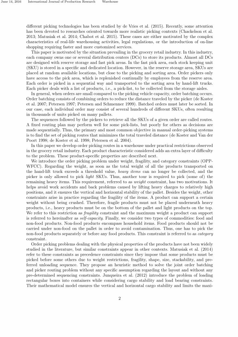
4.2.2 Branch-and-cut algorithms

Models F1 and F2 can be fed straightforwardly into a general purpose solver and solutions areobtained by branch-and-bound if the number of constraints (3.10), (3.18), (3.21) and (3.22) is notexcessive. However, for instances of realistic size, the number of these constraints is too large toallow a full enumeration and they must be dynamically generated throughout the search process.Indeed, polynomial constraints may be added a priori to the model while other constraints cannotbe generated a priori since their number is exponential.

The exact algorithm we present is a branch-and-cut scheme in which inequalities (3.10), (3.18),(3.21), and (3.22) are generated and added into the program whenever they are found to be violated.It works as follows. At a generic node of the search tree, a linear program containing the model witha subset of the subtour elimination constraints and relaxed integrality constraints is solved, a searchfor violated inequalities is performed, and some of these are added to the current program whichis then reoptimized. This process is reiterated until a feasible or dominated solution is reached, oruntil there are no more cuts to be added. At this point, branching on a fractional variable occurs.We provide a sketch of the branch-and-cut scheme in Algorithm 2. Note that for formulation F1,we apply Algorithm 2 but we skip the process to identify violated subtour elimination constraints(lines 8− 12) as connectivity requirements are ensured by constraints (3.4).

Algorithm 2 Branch-and-cut algorithm1: Subproblem solution: Solve the LP relaxation of the current node2: Termination check:3: if there are no more nodes to evaluate then4: Stop5: else6: Select one node from the branch-and-cut tree7: end if8: while the solution of the current LP relaxation contains subtours do9: Identify connected components as in Padberg and Rinaldi (1991)

10: Add violated subtour elimination constraints11: Subproblem solution. Solve the LP relaxation of the current node12: end while13: if the solution contains no disconnected components then14: Apply Algorithms 3 and 4, and add violated cuts15: end if16: if the solution of the current LP relaxation is integer then17: Go to the termination check18: else19: Branching: branch on one of the fractional variables20: Go to the termination check21: end if

In this branch-and-cut algorithm, weight, and fragility inequalities are used as cutting planesto strengthen the linear programming relaxation at each node of the branch-and-bound tree. Con-straints (3.10), (3.21), and (3.22) cannot be generated a priori since their number is exponential.These are initially relaxed and dynamically generated as cuts as they are found to be violated.

When model F1 without weight constraints (3.10) (similarly with (3.22) for F2) is solved, twosituations can occur. The first one consists of finding an integer solution. Then one can easily verifyif the picking tour exceeds the weight limit L or the self-capacity wi by calculating the cumulativeweight of a set S. In the second case, when the solution is fractional, one can identify connectedcomponents by means of the maximum flow algorithm as in Padberg and Rinaldi (1991). This

13


procedure, sketched in Algorithm 3, consists of constructing an auxiliary graph as follows. First, anode i is selected. Then the node j associated with the maximum flow value leaving i is identifiedand added to the set S. We check whether the sum of weights of the products included in S, referredto by qS , respects the threshold L. If it exceeds this limit, we add cuts to forbid such solution. Thisis achieved by adding the appropriate constraints (3.10) for the capacity indexed formulation, and(3.22) for the two-index flow formulation associated with the nodes in S.

Similarly, in Algorithm 4, we describe the procedure used to dynamically generate constraints(3.21). We identify a subset S such that it respects the fragility constraints. Otherwise, we add theviolated constraints associated with the nodes in S.

Algorithm 3 Weight constraints algorithm1: for i = 1 to m do2: S = i3: j∗ = argmaxk∈V ′\Sxik4: S = S ∪ j∗5: if qS > L and qS ≤ Q then6: for l ∈ S do7: if the solution violates (3.10) (or (3.22)) then8: Add weight constraints (3.10) (or (3.22))9: end if

10: end for11: end if12: if qS > Q then13: Continue to next i from step 114: else15: Go to Step 316: end if17: end for

5. Computational experiments

In this section, we provide details on the implementation, benchmark instances, and describe theresults of extensive computational experiments. Implementation and hardware information is pro-vided in Section 5.1. The description of the benchmark instances is presented in Section 5.2, followedby the results of our computational experiments. Heuristic results are presented in Section 5.3 andthe results of experiments carried out in order to assess the performance of the proposed exactmethods are presented in Section 5.4.

5.1 Implementation details

All the formulations described in Section 3 and the algorithms described in Section 4 were imple-mented in C++. The branch-and-cut algorithm uses the CVRPSEP library (Lysgaard 2003) forthe sub-tours elimination constraints, the newly proposed cutting methods, and IBM CPLEX Con-cert Technology 12.6 as the branch-and-bound solver. All computations were executed on machinesequipped with two Intel Westmere EP X5650 six-core processors running at 2.667 GHz, and with upto 8 GB of RAM installed per node running the Scientific Linux 6.3. All algorithms were provideda time limit of 7200 seconds.

14


Algorithm 4 Fragility constraints algorithm1: for i = 1 to m do2: if i is a fragile product then3: S = i, best = i4: while stop criterion is not met do5: j∗ = argmaxk∈V ′\Sxbest,k)6: if xbest,k < 0.5 then7: Stop8: end if9: S = S ∪ j∗, Best=j

10: if qS ≤ Q and qS > wi then11: if the solution violates (3.21) then12: Add fragility constraints (3.21)13: end if14: end if15: if qS > Q then16: Stop17: end if18: end while19: end if20: end for

5.2 Data sets generation

Since no data sets are available for the OPP-WFCC, we have created three groups of instances torepresent different configurations and combinations of the new features introduced in this paper.To reflect common practice, non-food items are grouped in the same aisle(s). In the first group ofinstances, called G1, only one side of the first aisle is dedicated to non-food items, whereas all fragileand non-fragile products are randomly placed throughout the warehouse. In the second group ofinstances (G2), we split the picking area in two symmetric zones. This allows non-food items tobe placed in the lateral extremities of the warehouse. All remaining items are placed randomlyelsewhere. In the third group (G3), non-food items are placed in the extremities like in G2, butsolid products (SP), i.e., non-fragile, with large self-capacity are grouped together in the sectionsclose to the I/O point. These three types of layouts are illustrated in Figure 4.

NFNFNFNF

NFNFNFNF

NFNFNFNF

NFNFNFNF

IIII////OOOO

NFNFNFNF

NFNFNFNF

NFNFNFNF

NFNFNFNF

IIII////OOOO

NFNFNFNF

NFNFNFNF

NFNFNFNF

NFNFNFNF

NFNFNFNF

SPSPSPSP

NFNFNFNF

NFNFNFNF

NFNFNFNF

IIII////OOOO

NFNFNFNF

NFNFNFNF

NFNFNFNF

NFNFNFNF

SPSPSPSP SPSPSPSP SPSPSPSP

SPSPSPSP SPSPSPSP SPSPSPSP SPSPSPSP

G1G1G1G1:::: oneoneoneone zonezonezonezone G2G2G2G2:::: twotwotwotwo zoneszoneszoneszones G3G3G3G3:::: twotwotwotwo zoneszoneszoneszones andandandand solidssolidssolidssolids inininin firstfirstfirstfirst sectionssectionssectionssections

NFNFNFNF:::: nonnonnonnon----foodfoodfoodfood productproductproductproductSPSPSPSP:::: solidsolidsolidsolid productproductproductproduct

Figure 4. Schematic representation of the three groups of instances

In each group of instances, we have kept the same proportion of food and non-food products, andranges of weight and self-capacity. The generator has a 50% probability to create a fragile product.Each fragile product has a 2/3 probability to be a food product and 1/3 to be non-food. A non-

15


fragile product, food or otherwise, has a weight between five and 50 kg, and infinite self-capacity.A fragile product has a weight between one and 10 kg, and a self-capacity between five and 50 kg.

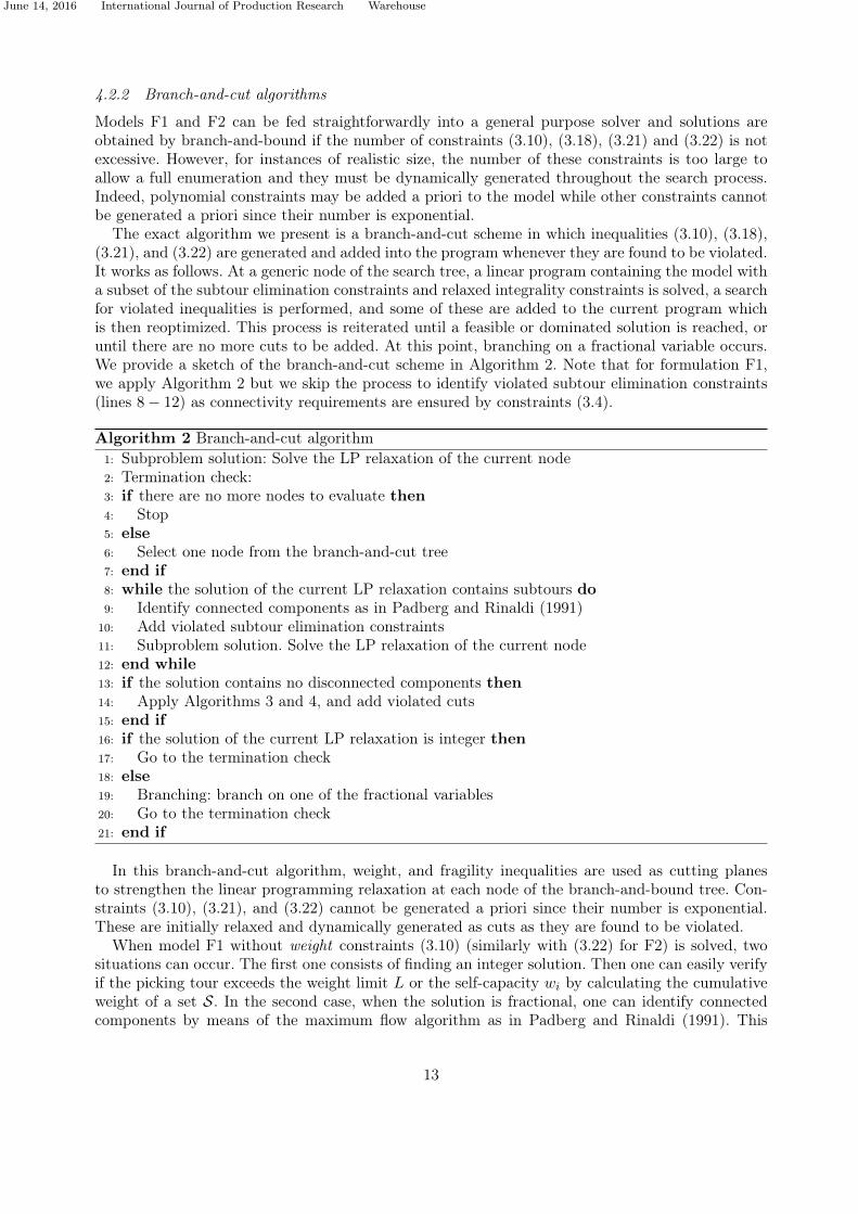
The general characteristics of this large test bed are summarized in Table 1. An instance ischaracterized by the number of picks, the number of aisles, and the capacity of the picking vehicles.The number of SKU to be picked is between 20 and 100, by steps of 10. The number of aisles isequal to 3, 4, 5, 6 or 7, with the I/O point located in the middle of the warehouse. The capacity ofthe pallet may take the value 150 or 250. In total, there are 270 different parameter combinationsrepresented in Table 1. For each combination, we have generated randomly three instances, fortest bed of 810 distinct instances. Recall that each aisle side contains 20 storage locations and thenumber of SKU per warehouse depends on the number of aisles. Regarding the parameters values,we have used the following physical distance parameters: α = 10, β = 5, γ = 15, and Ω = 5.

Table 1. General characteristics of the generated test bed

Parameter Variations Values

group 3 G1, G2, G3# of picks 9 20, 30, 40, 50, 60, 70, 80, 90, 100# of aisles 5 3, 4, 5, 6, 7capacity of the pallet 2 150, 250

5.3 Heuristic results

This section presents the results of extensive computational experiments of the five heuristic al-gorithms presented in Section 4.1 for the test bed containing 810 instances. Table 2 presents thesolutions of the heuristic algorithms for all the three groups of instances. Specifically, for eachheuristic, group, and pallet capacity, and for each number of pickups we provide the total distancewhich is the average over 15 instances, i.e., three instances for each scenario. We also provide theaverage distance over each group.

The best average results of classical heuristics are underlined for each capacity and each group. Interms of computational times required by the different heuristic algorithms, the CPU time needed isless than one second for instances with 100 pickups and seven aisles. The classical heuristics resultspresented in Table 2 highlight that their performance slightly differ over the three instances groups.The mid-point heuristic is most likely less effective than the other heuristics. For the first group,the combined heuristic outperforms the other three. For G2, the S-shape heuristic is the best one.Finally, for G3, the largest gap heuristic yields the best results. These results hold for both capacityscenarios. More generally, the four classical heuristics yielded very similar solutions, whereas thesemay be significantly enhanced by the ALNS metaheuristic.

A richer and more intricate metaheuristic, such as the ALNS, significantly improves the solution,as shown in Table 2. The average solution is reduced by almost 50% for all groups. This maybe explained by the fact that the ALNS metaheuristic provides more compact solutions with fewerpicking tours and much shorter distances, thanks to its intensification and diversification procedures.Regarding the running time, the ALNS improves the solution quality with no significant timeincrease. The average running time is around 60 seconds for the largest instances with 100 pickupsand 7 aisles. As expected, increasing the capacity of the pallet (as done in the second scenario)reduces the distance traversed, and this for all heuristics. Moreover, being the most advanced one,the ALNS better exploits this extra capacity and reduces distances significantly.

16


Table 2. Average heuristic results on instances with Q = 150 and Q = 250

# Q = 150 Q = 250pickups S-shape Mid point L-Gap Combined ALNS S-shape Mid point L-Gap Combined ALNS

G1 20 2169.00 2224.00 2205.67 2016.67 1234.33 1917.00 2036.00 1826.33 1852.00 1082.3330 2949.00 3014.33 2902.33 2850.00 1555.33 2638.67 2891.67 2715.67 2443.67 1357.6740 3665.33 3812.33 3558.33 3611.67 1904.67 3075.67 3281.67 3145.33 2967.00 1552.6750 4075.67 4223.33 4126.00 3972.33 2135.33 3754.00 3917.67 3892.00 3562.33 1831.3360 5181.33 5114.33 4912.67 5023.33 2540.33 4357.67 4311.00 4240.67 4157.00 2063.3370 5694.67 5680.00 5409.00 5600.67 2739.33 4816.33 4935.33 4788.33 4615.00 2259.3380 6159.33 6135.00 6012.33 5750.33 3046.33 5329.00 5226.67 5215.67 5029.33 2382.3390 7011.67 6878.00 6886.67 6877.00 3408.33 5651.67 5919.67 5579.00 5331.00 2580.00100 7663.67 7550.00 7452.67 7147.00 3716.67 5981.00 6084.33 6045.67 5897.33 2738.00

Average 4952.19 4959.04 4829.52 4761.00 2475.63 4169.00 4289.33 4160.96 3983.85 1983.00

G2 20 2231.00 2441.00 2288.00 2213.00 1290.67 1959.33 2171.33 2077.00 1961.33 1171.0030 3093.33 3274.67 3154.67 2996.00 1641.33 2651.33 2950.00 2835.00 2747.00 1450.0040 3695.33 3757.67 3765.33 3728.33 1967.00 3398.33 3514.33 3527.00 3263.67 1693.6750 4150.00 4303.00 4295.33 4244.33 2219.67 3878.00 4322.33 3961.33 3814.67 1883.6760 5034.33 5403.00 5044.00 5249.33 2568.00 4445.67 4469.33 4487.00 4473.33 2135.3370 5608.67 5874.67 5714.67 5648.00 2797.00 4667.33 5089.33 4858.67 4993.33 2351.0080 6048.00 6376.33 6132.67 6142.67 3133.33 5201.00 5223.00 5250.67 5218.33 2446.6790 6921.67 7087.67 6973.67 6719.00 3466.33 5448.67 5808.00 5469.00 5519.00 2665.33100 7453.67 7680.67 7338.00 7625.67 3773.67 6180.67 6239.00 6042.67 6074.00 2764.44

Average 4915.11 5133.19 4967.37 4951.81 2539.67 4203.37 4420.74 4278.70 4229.41 2062.35

G3 20 2311.00 2438.33 2205.67 2199.67 1279.67 2047.67 2147.33 2003.33 2025.67 1195.0030 2977.00 3183.00 3071.33 2982.67 1620.67 2686.00 2990.00 2695.00 2742.00 1439.0040 3590.00 3714.00 3455.67 3732.00 1919.00 3370.33 3484.67 3356.00 3230.67 1676.6750 4173.67 4400.00 4110.67 4248.67 2158.33 3736.33 4113.33 3758.33 3908.33 1862.3360 4911.00 5084.33 4980.33 5099.67 2487.33 4387.33 4501.33 4325.67 4455.00 2102.6770 5415.33 5651.00 5428.00 5779.00 2707.33 4660.00 5265.00 4734.00 4980.33 2328.6780 5949.00 6030.67 5904.67 6111.67 3011.67 5410.33 5243.00 5113.00 5224.33 2377.0090 6892.33 6828.33 6857.67 6738.00 3327.00 5371.67 5764.33 5353.00 5568.00 2606.33100 7262.67 7380.33 7132.67 7786.67 3586.67 5959.33 6125.33 5826.33 6023.33 2764.67

Average 4831.33 4967.78 4794.07 4964.22 2455.30 4181.00 4403.81 4129.41 4239.74 2039.15

Overall average 4899.54 5020.00 4863.65 4892.35 2490.20 4184.46 4371.30 4189.69 4151.00 2028.16

5.4 Exact algorithms results

Tables 3 and 4 present the results of the best heuristic proposed (ALNS) compared to the resultsobtained by solving the two mathematical models, F1 and F2, when applying the branch-and-cutalgorithms with the proposed cutting planes.

For each instance group and for each number of pickups, we provide the average results over allthe instances and over all the number of aisles, with Q = 150 in Table 3 and Q = 250 in Table 4.We report the upper bound (UB) and the lower bound (LB) for models F1 and F2. We provide theaverage percentage gaps, given by the ratio (UB−LB

LB · 100). We also provide the average runningtime in seconds.

From Tables 3 and 4, we observe that the results provided by the ALNS metaheuristic areclose to the best UBs yielded by both models. For instance, when Q = 150, ALNS gives an overallaverage distance of 2496.83 compared to 2482.68 and 2479.07 for F1 and F2. This remark also holdswhen Q = 250. Moreover, the ALNS algorithm provides near-optimal solutions within very shortcomputing times (few seconds) compared to the time spent by both models to prove optimalityor to provide better UBs. However, deriving better results at the expense of longer run times wasone of our goals to provide the best possible results for the newly proposed testbed and serve thewarehousing research community.

A deeper analysis of the formulations shows that the solutions are tight, and the optimality gapis in average 9.35% when Q = 150 for F1, and 6.91% for F2. Model F2 proves optimality over allinstances with 20 pickups and almost all instances with 30 pickups within very short computingtimes. Both models had problems closing the gap and proving optimality for instances with morethan 30 pickups.

Note that the time limit of 7200 seconds is often exceeded by F1. This is due to the fact thatthe time spent to instantiate model F1 is also considered in the total time, and the size of modelF1 may become an issue when the instance size increases. For example, for instances including 100pickups, almost two hours are needed only to create the model.

Finally, it is important to notice that the subset sum algorithm presented in Section 4.2.1 was

17


able to reduce an average of 12.55% variables compared to a complete enumeration of all possiblevariables for model F1. In our test bed, we have observed a reduction of up to 23.56% in the numberof variables, and a minimum reduction of 5.87%.

Regarding the three groups of instances, we observe that the gap between the upper and lowerbounds is slightly lower for group G1 for both models. There are no major differences among groupsin terms of the traveled distance except for very small variations. Indeed, it seems more difficult tosolve instances where the products are placed in groups, in such a way as to facilitate the pickingwork.

Table 3. Average results of the exact algorithms per group of instances and number of pickups on instances with Q = 150

Group Pickups ALNS Time (s) Capacity indexed formulation (F1) Two-index formulation (F2)UB LB %Gap Time (s) UB LB %Gap Time (s)

G1 20 1251.00 1.53 1232.00 1232.00 0.00 118.27 1232.00 1232.00 0.00 8.0030 1568.00 3.33 1542.67 1521.86 1.37 1577.60 1542.67 1540.30 0.15 541.6040 1928.00 5.53 1892.67 1798.71 5.22 7278.67 1888.67 1873.72 0.80 1656.4050 2127.33 9.60 2120.67 1937.19 9.47 7604.07 2104.33 2031.58 3.58 5321.4060 2530.33 16.40 2529.33 2319.77 9.03 8678.60 2525.67 2380.87 6.08 7200.6770 2734.00 24.47 2733.33 2491.91 9.69 9527.27 2732.33 2595.60 5.27 7201.0080 3040.67 31.20 3038.33 2790.07 8.90 10031.27 3035.00 2854.34 6.33 7201.2090 3403.33 50.33 3402.67 3083.69 10.34 16523.53 3403.33 3153.14 7.93 7202.67100 3722.67 65.60 3722.67 3373.26 10.36 19710.80 3722.67 3426.66 8.64 7202.93

Average 2478.37 23.11 2468.26 2283.16 8.11 9005.56 2465.19 2343.13 5.21 4837.32

G2 20 1300.33 1.07 1287.67 1252.50 2.81 188.53 1287.67 1287.67 0.00 99.7330 1661.67 3.20 1627.67 1601.29 1.65 3185.60 1627.00 1626.52 0.03 1066.0740 2012.33 6.13 1962.67 1820.88 7.79 7140.73 1955.67 1890.01 3.47 4403.5350 2230.00 9.40 2221.33 1993.66 11.42 7946.80 2193.00 2079.29 5.47 6028.4760 2565.33 17.13 2557.00 2301.68 11.09 8804.27 2546.00 2371.23 7.37 6923.1370 2803.33 24.80 2797.33 2519.51 11.03 9967.53 2798.00 2574.98 8.66 7201.1380 3129.67 33.73 3129.33 2805.88 11.53 11105.93 3113.00 2848.36 9.29 7201.6090 3453.67 51.00 3453.67 3116.54 10.82 14786.20 3453.67 3165.65 9.10 7202.33100 3783.00 67.53 3781.00 3392.42 11.45 17634.47 3783.00 3420.28 10.60 7202.93

Average 2548.81 23.78 2535.30 2311.60 9.68 8973.34 2528.56 2362.66 7.02 5258.77

G3 20 1275.33 1.67 1253.00 1140.00 9.91 211.47 1253.00 1253.00 0.00 7.6730 1614.67 3.13 1592.33 1592.33 0.00 1559.87 1592.33 1586.33 0.38 850.0740 1958.33 5.60 1871.67 1781.19 5.08 6868.73 1879.33 1816.53 3.46 3475.0050 2139.67 8.87 2119.00 1939.38 9.26 7849.73 2109.33 1995.65 5.70 6013.2060 2490.67 16.27 2474.00 2206.25 12.14 8744.40 2473.00 2254.63 9.69 6729.3370 2706.67 20.80 2706.67 2431.64 11.31 9096.13 2702.67 2448.13 10.40 7201.0080 3042.33 31.00 3041.67 2678.45 13.56 11614.67 3041.67 2679.62 13.51 7201.8090 3360.67 43.13 3360.67 2991.94 12.32 12734.93 3358.67 3029.84 10.85 7201.80100 3581.33 66.87 3581.33 3188.99 12.30 16577.47 3581.33 3195.08 12.09 7202.13

Average 2463.30 21.93 2444.48 2216.69 10.28 8361.93 2443.48 2250.98 8.55 5098.00

Overall average 2496.83 22.94 2482.68 2270.48 9.35 8780.28 2479.07 2318.93 6.91 5064.70

Table 5 presents the number of optimal solutions obtained by both models over the 810 instances.These results are separated in groups of instances, number of aisles, and by the value of the capacityQ. This helps highlight the effect of each of these characteristics. In the first and second lineswe present the capacity indexed formulation F1 and the two-index formulation F2 with the twocapacities, Q = 150 and Q = 250. We then present the results for each group of instances and eachnumber of aisles. The number of optimal solutions is slightly higher with F2. This corroborates theresults already observed from the gaps and running time of these models. A transversal analysis ofTables 3, 4, and 5 points out again the difficulty of the problem. We observe that the best exactalgorithm is able to prove optimality for only 27% of the instances.

Table 6 presents a deeper statistical comparison between the proposed formulations. For eachmodel, we provide averages for the percentage optimality gap, the computation time in seconds, thenumber of variables, and constraints generated along with the number of cuts added to fractionaland integer solutions, and finally the number of nodes explored in the branch-and-bound tree. Thelast column of the table shows the relative difference of F1 with respect to F2.

The first outstanding result from Table 6 is related to the huge number of variables and constraintsgenerated in F1. These two figures are more than 100 times higher than the number of variablesand constraints generated in F2. Although the subset sum algorithm helps decreasing the size ofF1 by removing irrelevant variables, the size of formulation F1 remains huge compared to F2 andrequires much more time to load the instance and create the model.

18


Table 4. Average results of the exact algorithms per group of instances and number of pickups on instances with Q = 250

Group Pickups ALNS Time (s) Capacity indexed formulation (F1) Two-index formulation (F2)UB LB %Gap Time (s) UB LB %Gap Time (s)

G1 20 1093.67 1.73 1064.33 1048.65 1.50 1644.87 1063.33 1063.33 0.00 1.0730 1388.00 4.40 1360.33 1314.20 3.51 4645.33 1355.67 1355.67 0.00 45.8040 1568.67 6.87 1559.33 1422.70 9.60 7523.00 1530.33 1517.27 0.86 2241.0050 1859.33 12.07 1858.67 1584.14 17.33 8551.40 1836.00 1701.57 7.90 7081.7360 2057.67 20.33 2057.00 1746.16 17.80 12133.93 2016.33 1847.55 9.14 7065.6770 2236.67 31.80 2236.67 1911.78 16.99 14281.20 2228.00 1987.49 12.10 7200.9380 2387.00 46.07 2387.00 1999.96 19.35 17920.47 2377.33 2043.08 16.36 7201.1390 2568.00 73.67 2568.00 2157.94 19.00 35708.87 2567.33 2214.82 15.92 7202.07100 2716.67 86.27 2716.67 2283.53 18.97 41148.93 2716.00 2323.99 16.87 7201.73

Average 1986.19 31.47 1978.67 1718.78 15.12 15950.89 1965.59 1783.86 10.19 5026.79

G2 20 1209.33 1.67 1164.67 1149.44 1.32 2309.47 1164.67 1164.67 0.00 0.3330 1499.67 3.87 1470.33 1357.62 8.30 5233.27 1448.00 1444.69 0.23 529.0740 1728.67 7.40 1714.67 1526.73 12.31 8008.13 1699.00 1641.20 3.52 4543.8050 1935.67 12.07 1935.67 1613.44 19.97 9346.67 1891.33 1673.86 12.99 6787.1360 2179.67 22.80 2179.67 1810.35 20.40 12049.20 2141.67 1876.63 14.12 6893.5370 2379.67 31.20 2377.67 1973.70 20.47 15551.13 2354.00 2005.31 17.39 7201.2780 2473.00 46.27 2473.00 2037.14 21.40 21498.93 2473.00 2072.88 19.30 7201.5390 2694.67 65.47 2694.67 2230.08 20.83 33595.00 2694.00 2266.36 18.87 7202.27100 2825.33 80.07 2825.33 2351.37 20.16 40648.80 2823.33 2356.54 19.81 7202.47

Average 2102.85 30.09 2092.85 1783.32 17.36 16471.18 2076.56 1833.57 13.25 5284.60

G3 20 1235.33 1.53 1193.33 1177.85 1.31 2571.73 1193.00 1193.00 0.00 0.6030 1481.00 4.00 1452.00 1357.24 6.98 4982.13 1441.00 1441.00 0.00 178.5340 1730.00 6.87 1720.00 1508.52 14.02 7646.07 1676.00 1633.55 2.60 3854.4750 1876.00 13.27 1876.00 1602.06 17.10 8903.73 1856.67 1680.63 10.47 6233.3360 2149.00 20.27 2149.00 1795.72 19.67 11513.80 2106.33 1817.12 15.92 7200.7370 2321.67 28.13 2321.67 1938.48 19.77 14725.33 2304.33 1962.90 17.39 7201.0780 2384.67 44.53 2384.67 2008.36 18.74 22755.27 2383.33 2007.33 18.73 7201.6790 2641.00 55.67 2641.00 2179.95 21.15 28728.27 2640.33 2202.66 19.87 7201.73100 2780.67 80.00 2780.00 2311.15 20.29 35836.53 2778.67 2291.00 21.29 7201.60

Average 2066.59 28.25 2057.52 1764.37 16.61 15295.87 2042.19 1803.24 13.25 5141.53

Overall average 2051.88 29.94 2043.01 1755.49 16.38 15905.98 2028.11 1806.89 12.24 5150.97

Table 5. Number of optimal solutions per group of instances and capacity of the truckG1 G2 G3

Capacity 3 4 5 6 7 Total 3 4 5 6 7 Total 3 4 5 6 7 Total Total

F1 Q=150 6 7 5 6 6 30 4 5 4 6 6 25 8 7 6 7 5 33 88Q=250 8 9 10 11 8 46 8 7 9 8 9 41 8 8 9 9 7 41 128

F2 Q=150 5 4 4 4 6 23 4 4 4 3 5 20 4 4 3 4 5 20 63Q=250 9 9 8 9 9 44 6 7 6 8 10 37 7 8 7 9 10 41 122

However, F1 uses almost no cuts during the search process to limit the size of the solution whileF2 invokes a huge number of cuts for both fractional and integer solutions. Indeed, over all instances,F2 uses on average 316.2 cuts on fractional solutions and 9703.5 on integer ones. This is due tothe fact that F1 does not need to add sub-tours elimination constraints or self-capacity constraintsduring the search process. Moreover, for both models and on instances with more than 40 pickups,the number of visited nodes gradually decreases while the instances size increases. This is due tothe increasing number of cuts generated while the instances size increases and then a smaller treesize is explored. This shows that the average number of visited nodes in F1 is less than the numberof visited nodes in F2 by 33%. These results clearly show that formulation F1 is again outperformedby formulation F2.

Table 6. Statistical comparison of models F1 and F2 over all instances per number of pickupsPickups 20 30 40 50 60 70 80 90 100 Average vs. F2

F1

% Gap 3.2 4.1 9.2 14.5 15.5 15.0 15.7 15.8 15.6 12.0 42%Time (s) 1174.1 3530.6 7410.9 8367.1 10320.7 12191.4 15821.1 23679.5 28592.8 12343.1 142%

# Variables 37479.6 72740.4 130246.9 203011.6 280638.7 384998.3 497471.6 665514.9 793555.8 340628.6 10528%# Constraintes 12962.8 23821.5 37205.6 57058.8 75440.1 98905.7 130409.9 159564.4 194357.4 87747.3 11308%Fractional cuts 0.6 1.1 1.4 0.2 0.1 0.2 0.1 0.0 0.0 0.4 -100%

Integer cuts 12.6 17.2 23.2 10.9 7.3 5.5 6.7 2.3 3.3 9.9 -100%# Nodes 12998.2 32487.2 31799.1 13686.6 4279.6 2436.6 1504.5 373.6 320.4 11098.4 -33%

F2

% Gap 0.0 0.2 2.7 8.0 10.9 12.0 14.1 13.8 14.9 8.5Time (s) 19.6 535.2 3362.4 6244.2 7002.2 7201.1 7201.5 7202.1 7202.3 5107.8

# Variables 330.9 703.7 1218.8 1895.9 2698.1 3691.6 4748.4 6121.6 7435.2 3204.9# Constraintes 101.5 198.8 312.9 486.3 671.4 880.7 1163.6 1378.6 1728.5 769.2Fractional cuts 96.7 277.4 455.4 581.3 476.9 283.7 273.4 206.9 193.9 316.2

Integer cuts 128.5 1144.2 5485.5 10890.1 14157.9 14544.8 14606.4 13246.6 13127.8 9703.5# Nodes 1838.3 19307.3 35759.4 34536.0 19465.7 14024.2 10649.1 6882.4 5773.8 16470,7

19


6. Conclusions

We have tackled a real-world-based and rich order picking problem arising in the grocery retailindustry which, to our knowledge, was studied here for the first time. This practical problemextended classical warehousing problems by incorporating more challenges regarding the physicalcharacteristics of the products to be picked. Specifically, products can support a maximum weightwhen being transported on a lift-truck used for warehouse picking, some products are more fragilethan others, and products belonging to food and non-food categories must be picked in a given ordersuch as to avoid contamination. We have adapted four classical order picking heuristics from thewarehousing literature to handle these new features. Notably, we have shown how the S-shape, thelargest gap, the mid point, and the combined heuristics can yield feasible solutions within very shortcomputation times. Moreover, we have also proposed a more powerful metaheuristic, ALNS, whichoutperforms the best results obtained by the four heuristics. We have presented two mathematicalmodels including known and new valid inequalities for this challenging picking problem. The first oneis the capacity-indexed formulation, which is a based compact single commodity flow using binaryvariables to indicate the flow on each arc. The second formulation is a two-index flow formulation,in which individual hand-lift trucks are not explicitly identified. We have proposed exact algorithmsfor their resolution.

We have tested the proposed heuristics, metaheuristic, and the two formulations on large sets ofnewly generated and realistic instances. The results show the effectiveness of the proposed heuristicsin finding high-quality solutions within a negligible computation time. The solutions provided by theALNS metaheuristic dominated those from the other heuristics, as it traversed smaller distances dueto fewer tours. Moreover, we have been able to prove optimality for several instances and to obtainbetter solutions and tight gaps with two mathematical models that were solved with classical andad-hoc valid inequalities and cutting planes. Extensive tests have shown that the proposed exactalgorithms outperformed the solutions of the heuristic algorithms. Moreover, we have shown thatthe two-index formulation outperforms the capacity-indexed formulation for this problem. The mostremarkable conclusion for this work is that the running times of the heuristics are very low, andthose of the exact algorithms are still acceptable, allowing for their usage in practical applications.

Our future works aim to show how the proposed solution methods can be adapted to cover avariety of other warehousing applications, in other industries and under different assumptions. Inaddition, there might be a strong correlation between the instances characteristics, e.g., warehousedesign, number of aisles, capacity of the truck, and the results obtained. Consequently, more researchis needed to demonstrate such interactions through design experiments, as they are supposed tosignificantly help find the best warehouse design with respect to the routing policy under differentconditions. Similar work has been already performed in Chackelson et al. (2013). Future researchthat supports this study may include more computational experiments to assess the impact of eachprecedence constraint on the performance of the heuristic and exact algorithms. Previous studiesevaluating the impact of different operating conditions on the route distance exist, e.g., Petersen(1997), Petersen and Schmenner (1999).

Acknowledgments

This research was partly supported by grants 2014-05764 and 0172633 from the Canadian Natu-ral Sciences and Engineering Research Council. This support is gratefully acknowledged. We alsothank Calcul Québec for providing computing facilities. We also thank Calcul Québec for providingcomputing facilities. We thank an associate editor and two anonymous referees for their commentson an earlier version of this paper.

20


References

K. B. Ackerman. Practical Handbook of Warehousing. Springer Science & Business Media, New York, 2013.M. Bortolini, M. Faccio, M. Gamberi, and R. Manzini. Diagonal cross-aisles in unit load warehouses to

increase handling performance. International Journal of Production Economics, 170:838–849, 2015.T. Chabot, L. C. Coelho, J. Renaud, and J.-F. Côté. Mathematical models, heuristic and exact method for

order picking in 3d-narrow aisles. Technical Report CIRRELT-2015-18, Québec, Canada, 2015.C. Chackelson, A. Errasti, D. Ciprés, and F. Lahoz. Evaluating order picking performance trade-offs by con-

figuring main operating strategies in a retail distributor: a design of experiments approach. InternationalJournal of Production Research, 51(20):6097–6109, 2013.

D. M.-H. Chiang, C.-P. Lin, and M.-C. Chen. The adaptive approach for storage assignment by mining dataof warehouse management system for distribution centres. Enterprise Information Systems, 5(2):219–234,2011.

J-F. Cordeau and G. Laporte. The dial-a-ride problem: models and algorithms. Annals of OperationsResearch, 153(1):29–46, 2007.

R. de Koster and E. Van der Poort. Routing orderpickers in a warehouse: a comparison between optimaland heuristic solutions. IIE Transactions, 30(5):469–480, 1998.

R. de Koster, E. S. Van der Poort, and K. J. Roodbergen. When to apply optimal or heuristic routing oforderpickers. In B. Fleischmann, J. A. E. E. Van Nunen, M.G. Speranza, and P. Stähly, editors, Advancesin Distribution Logistics, pages 375–401. Springer, Berlin, 1998.

R. de Koster, T. Le-Duc, and K. J. Roodbergen. Design and control of warehouse order picking: A literaturereview. European Journal of Operational Research, 182(2):481–501, 2007.

J. de Vries, R. de Koster, and D. Stam. Exploring the role of picker personality in predicting pickingperformance with pick by voice, pick to light and RF-terminal picking. International Journal of ProductionResearch, pages 1–15, 2015.

R. Dekker, M. B. M. De Koster, K. J. Roodbergen, and H. Van Kalleveen. Improving order-picking responsetime at ankor’s warehouse. Interfaces, 34(4):303–313, 2004.

J. Gu, M. Goetschalckx, and L. F. McGinnis. Research on warehouse design and performance evaluation:A comprehensive review. European Journal of Operational Research, 203(3):539–549, 2010.

R. W. Hall. Distance approximations for routing manual pickers in a warehouse. IIE Transactions, 25(4):76–87, 1993.

S. Henn, S. Koch, and G. Wäscher. Order batching in order picking warehouses: A survey of solutionapproaches. In R. Manzini, editor, Warehousing in the Global Supply Chain, pages 105–137. Springer,London, 2012.

M. Hompel and T. Schmidt. Warehouse Management: Automation and Organisation of Warehouse andOrder Picking Systems. Springer, Berlin, 2006.

L. Junqueira, R. Morabito, and D. S. Yamashita. Three-dimensional container loading models with cargostability and load bearing constraints. Computers & Operations Research, 39(1):74–85, 2012.

R. Lahyani, F. Semet, and B. Trouillet. Vehicle routing problems with scheduling constraints. In Meta-heuristics for Production Scheduling, pages 433–463. Wiley Online Library, United Kingdom, 2014.

R. Lahyani, L. C. Coelho, and J. Renaud. Alternative formulations and improved bounds for the multi-depotfleet size and mix vehicle routing. Technical Report CIRRELT-2015-36, Québec, Canada, 2015.

G. Laporte. Generalized subtour elimination constraints and connectivity constraints. Journal of the Oper-ational Research Society, 37(5):509–514, 1986.

W. Lu, D. McFarlane, V. Giannikas, and Q. Zhang. An algorithm for dynamic order-picking in warehouseoperations. European Journal of Operational Research, 248(1):107–122, 2016.

J. Lysgaard. CVRPSEP: A package of separation routines for the capacitated vehicle routing problem.Department of Management Science and Logistics, Aarhus School of Business, Denmark, 2003.

R. Manzini. Warehousing in the Global Supply Chain. Springer, London, 2012.M. Matusiak, R. de Koster, L. Kroon, and J. Saarinen. A fast simulated annealing method for batching

precedence-constrained customer orders in a warehouse. European Journal of Operational Research, 236(3):968–977, 2014.

C. P. Medard and N. Sawhney. Airline crew scheduling from planning to operations. European Journal ofOperational Research, 183(3):1013–1027, 2007.

M. W. Padberg and G. Rinaldi. A branch-and-cut algorithm for the resolution of large-scale symmetric

21


traveling salesman problems. SIAM Review, 33(1):60–100, 1991.J. Park and B.-I. Kim. The school bus routing problem: A review. European Journal of Operational Research,

202(2):311–319, 2010.A. Pessoa, E. Uchoa, and M. V. S. Poggi de Aragão. A robust branch-cut-and-price algorithm for the

heterogeneous fleet vehicle routing problem. Networks, 54(4):167–177, 2009.C. G. Petersen. An evaluation of order picking routeing policies. International Journal of Operations &

Production Management, 17(11):1098–1111, 1997.C. G. Petersen and G. R. Aase. A comparison of picking, storage, and routing policies in manual order

picking. International Journal of Production Economics, 92(1):11–19, 2004.C. G. Petersen and R. W. Schmenner. An evaluation of routing and volume-based storage policies in an

order picking operation. Decision Sciences, 30(2):481–501, 1999.C. G. Petersen, G. R. Aase, and D. R. Heiser. Improving order-picking performance through the implemen-

tation of class-based storage. International Journal of Physical Distribution & Logistics Management, 34(7):534–544, 2004.

J. C. Picard and M. Queyranne. The time-dependent traveling salesman problem and its application to thetardiness problem in one-machine scheduling. Operations Research, 26(1):86–110, 1978.

M. V. S. Poggi de Aragão and E. Uchoa. New exact algorithms for the capacitated cehicle routing problem.In P. Toth and D. Vigo, editors, Vehicle Routing: Problems, Methods, and Applications, pages 59–86.MOS-SIAM Series on Optimization, Philadelphia, 2014.

J.-Y. Potvin and J.-M. Rousseau. A parallel route building algorithm for the vehicle routing and schedulingproblem with time windows. European Journal of Operational Research, 66(3):331–340, 1993.

K. J. Roodbergen and R. de Koster. Routing order pickers in a warehouse with a middle aisle. EuropeanJournal of Operational Research, 133(1):32–43, 2001.

S. Ropke and D. Pisinger. An adaptive large neighborhood search heuristic for the pickup and deliveryproblem with time windows. Transportation Science, 40(4):455–472, 2006.

P. Shaw. A new local search algorithm providing high quality solutions to vehicle routing problems. Technicalreport, APES Group, Dept of Computer Science, University of Strathclyde, Glasgow, Scotland, UK, 1997.

J. A. Tompkins, J. A. White, Y. A. Bozer, and J. M. A. Tanchoco. Facilities Planning. John Wiley & Sons,New York, 2010.

P. Toth and D. Vigo. The family of vehicle routing problem. In P. Toth and D. Vigo, editors, Vehicle Routing:Problems, Methods, and Applications, pages 1–23. MOS-SIAM Series on Optimization, Philadelphia, 2014.

G. Wäscher. Order picking: a survey of planning problems and methods. In H. Dyckhoff, R. Lackes, andJ. Reese, editors, Supply Chain Management and Reverse Logistics, pages 323–347. Springer, Berlin, 2004.

E. E. Zachariadis, C. D. Tarantilis, and C. T. Kiranoudis. The vehicle routing problem with simultane-ous pick-ups and deliveries and two-dimensional loading constraints. European Journal of OperationalResearch, 251(2):369–386, 2016.

22

order picking problems under weight, fragility, and

Documents