orbital mechanics for engineering … engineering... · solutions manual to accompany orbital...
TRANSCRIPT
SOLUTIONS MANUAL
to accompany
ORBITAL MECHANICS FOR ENGINEERING STUDENTS
Howard D. CurtisEmbry-Riddle Aeronautical University
Daytona Beach, Florida

Solutions Manual Orbital Mechanics for Engineering Students Chapter 1
1
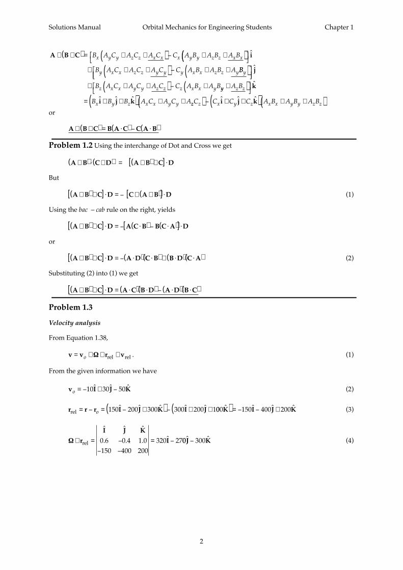
Problem 1.1(a)
A A i j k i j k
i
⋅ = + +( ) ⋅ + +( )= ⋅
A A A A A A
A
x y z x y z
x
ˆ ˆ ˆ ˆ ˆ ˆ
ˆ AA A A A A A A Ax y z y x y z zˆ ˆ ˆ ˆ ˆ ˆ ˆ ˆi j k j i j k+ +( ) + ⋅ + +( ) + kk i j k
i i i j
⋅ + +( )= ⋅( ) + ⋅( ) +
A A A
A A A
x y z
x x y
ˆ ˆ ˆ
ˆ ˆ ˆ ˆ2 AA A A A A A Ax z y x y yˆ ˆ ˆ ˆ ˆ ˆi k j i j j⋅( )
+ ⋅( ) + ⋅( ) +2
zz
z x z y zA A A A A
ˆ ˆ
ˆ ˆ ˆ ˆ
j k
k i k j
⋅( )
+ ⋅( ) + ⋅( ) + 2 ˆ ˆk k⋅( )
= ( ) + ( ) + ( )
+A A A A A A Ax x y x z y
2 1 0 0 xx y y z z x z y zA A A A A A A A0 1 0 0 02( ) + ( ) + ( )
+ ( ) + ( ) + 22
2 2 2
1( )
= + +A A Ax y z
But, according to the Pythagorean Theorem, A A A Ax y z
2 2 2 2+ + = , where A = A , the magnitude of
the vector A . Thus A A⋅ = A2 .
(b)
A B C A
i j k
i j k
⋅ ×( ) = ⋅
= + +
ˆ ˆ ˆ
ˆ ˆ ˆ
B B B
C C C
A A A
x y z
x y z
x y z(( ) ⋅ −( ) − −( ) + −ˆ ˆ ˆi j kB C B C B C B C B C B Cy z z y x z z x x y y x(( )
= −( ) − −( ) + −A B C B C A B C B C A B Cx y z z y y x z z x z x y BB Cy x( )or
A B C⋅ ×( ) = + + − − −A B C A B C A B C A B C A B C A B Cx y z y z x z x y x z y y x z z y x (1)
Note that A B C C A B×( ) ⋅ = ⋅ ×( ) , and according to (1)
C A B⋅ ×( ) = + + − − −C A B C A B C A B C A B C A B C A Bx y z y z x z x y x z y y x z z y x (2)
The right hand sides of (1) and (2) are identical. Hence A B C A B C⋅ ×( ) = ×( ) ⋅ .
(c)
A B C i j k
i j k
× ×( ) = + +( ) ×A A A B B B
C C Cx y z x y z
x y z
ˆ ˆ ˆˆ ˆ ˆ
==
− − −
=
ˆ ˆ ˆi j k
A A A
B C B C B C B C B C B C
A
x y z
y z z y z x x y x y y x
yy x y y x z z x x z z y z zB C B C A B C B C A B C B−( ) − −( )
+ −i CC A B C B C
A B C B C A
y x x y y x
x z x x z
( ) − −( )
+ −( ) −
ˆ
j
yy y z z y
y x y z x z y y x z
B C B C
A B C A B C A B C A
−( )
= + − −
k
BB C A B C A B C A B C A B C
A
z x x y x z y z x x y z z y( ) + + − −( )+
ˆ ˆi j
xx z x y z y x x z y y z
x y y z z
B C A B C A B C A B C
B A C A C
+ − −( )= +
k
(( ) − +( )
+ +( ) −C A B A B B A C A C C A Bx y y z z y x x z z y xi xx z z
z x x y y z x x y y
A B
B A C A C C A B A B
+( )
+ +( ) − +( )j
k
Add and subtract the underlined terms to get
Solutions Manual Orbital Mechanics for Engineering Students Chapter 1
2
A B C× ×( ) = + +( ) − + +B A C A C A C C A B A B A Bx y y z z x x x y y z z x x(( )
+ + +( ) − + +
i
B A C A C A C C A B A B Ay x x z z y y y x x z z yBB
B A C A C A C C A B A B
y
z x x y y z z z x x y
( )
+ + +( ) − +
j
yy z z
x y z x x y y
A B
B B B A C A C A
+( )
= + +( ) + +
ˆ
ˆ ˆ ˆ
k
i j k zz z x y z x x y y z zC C C C A B A B A B( ) − + +( ) + +( )ˆ ˆ ˆi j k
or
A B C B A C C A B× ×( ) = ⋅( ) − ⋅( )
Problem 1.2 Using the interchange of Dot and Cross we get
A B C D A B C D×( ) ⋅ ×( ) = ×( ) ×[ ] ⋅
But
A B C D C A B D×( ) ×[ ] ⋅ = − × ×( )[ ] ⋅ (1)
Using the bac – cab rule on the right, yields
A B C D A C B B C A D×( ) ×[ ] ⋅ = − ⋅( ) − ⋅( )[ ] ⋅
or
A B C D A D C B B D C A×( ) ×[ ] ⋅ = − ⋅( ) ⋅( ) + ⋅( ) ⋅( ) (2)
Substituting (2) into (1) we get
A B C D A C B D A D B C×( ) ×[ ] ⋅ = ⋅( ) ⋅( ) − ⋅( ) ⋅( )
Problem 1.3
Velocity analysis
From Equation 1.38,
v v r v= + × +o ΩΩ rel rel . (1)
From the given information we have
v I J Ko = − + −10 30 50ˆ ˆ ˆ (2)
r r r I J K I Jrel = − = − +( ) − + +o 150 200 300 300 200 1ˆ ˆ ˆ ˆ ˆ 000 150 400 200ˆ ˆ ˆ ˆK I J K( ) = − − + (3)
ΩΩ× = −
− −
= −r
I J K
Irel
ˆ ˆ ˆ
. . . ˆ0 6 0 4 1 0150 400 200
320 2700 300ˆ ˆJ K− (4)

Solutions Manual Orbital Mechanics for Engineering Students Chapter 1
3
v i j k
I J
rel = − + +
= − +
20 25 70
20 0 57735 0 57735
ˆ ˆ ˆ
. ˆ . ˆ ++( )+ − + +
0 57735
25 0 74296 0 66475 0
. ˆ
. ˆ . ˆ
K
I J .. ˆ
. ˆ . ˆ
078206
70 0 33864 0 47410
K
I
( )+ − − JJ K+( )0 81274. ˆ
so that
v I J Krel m s= − − + ( )53 826 28 115 47 300. ˆ . ˆ . ˆ (5)
Substituting (2), (3), (4) and (5) into (1) yields
v I J K I J K= − + −( ) + − −( ) + −10 30 50 320 270 300 53ˆ ˆ ˆ ˆ ˆ ˆ .. ˆ . ˆ . ˆ826 28 115 47 300I J K− +( )
v I J K
I
= − −
=
256 17 268 12 302 7
478 68 0 53516
. ˆ . ˆ . ˆ
. . ˆ −− −( ) ( )0 56011 0 63236. ˆ . J K m s
Acceleration analysis
From Equation 1.42,
a a r r v a= + × + × ×( ) + × +O rel rel rel relΩΩ ΩΩ ΩΩ ΩΩ2 (6)
Using the given data together with (4) and (5) we obtain
a I J Ko = + −25 40 15ˆ ˆ ˆ (7)
ΩΩ× = − −
− −
= −r
I J K
Irel
ˆ ˆ ˆ
. . . ˆ0 4 0 3 1 0150 400 200
340 ++ +230 205ˆ ˆJ K (8)
ΩΩ ΩΩ× ×( ) = −
− −
=r
I J K
rel
ˆ ˆ ˆ
. . . ˆ0 6 0 4 1 0320 270 300
390II J K+ −500 34ˆ ˆ (9)
2 2 0 6 0 4 1 053 826 28 115 47 3
ΩΩ× = −
− −
v
I J K
rel
ˆ ˆ ˆ
. . .
. . . 0002 9 151 82 206 38 399= − −( ). ˆ . ˆ . ˆI J K (10)
a i j k
I
rel = − +
= +
7 5 8 5 6 0
7 5 0 57735 0 57735
. ˆ . ˆ . ˆ
. . ˆ . ˆ . ˆ
. . ˆ . ˆ .
J K
I J
+( )− − + +
0 57735
8 5 0 74296 0 66475 0 0078206
6 0 0 33864 0 47410 0
ˆ
. . ˆ . ˆ .
K
I J
( )+ − − + 881274K( )
a I J Krel = − +8 6134 4 1649 8 5418. ˆ . ˆ . ˆ (11)
Substituting (7), (8), (9), (10) and (11) into (6) yields
a I J K I J K= + −( ) + − + +( ) +25 40 15 340 230 205 390ˆ ˆ ˆ ˆ ˆ ˆ ˆ ˆ ˆ
. ˆ . ˆ . ˆ
I J K
I J K
+ −( )+ − −
500 34
2 9 151 82 206 38 399(( )
+ − +( )8 6134 4 1649 8 5418. ˆ . ˆ . ˆI J K
Solutions Manual Orbital Mechanics for Engineering Students Chapter 1
4
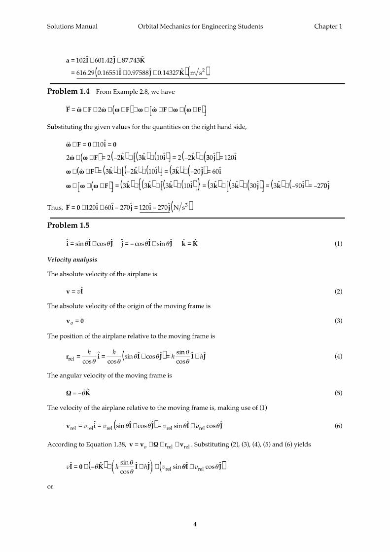
a I J K
I
= + +
= +
102 601 42 87 743
616 29 0 16551 0
ˆ . ˆ . ˆ
. . ˆ .. ˆ . ˆ 97588 0 14327J K+( ) ( )m s2
Problem 1.4 From Example 2.8, we have
F F F F F= × + × ×( ) + × × + × ×( ) ωω ωω ωω ωω ωω ωω ωω2
Substituting the given values for the quantities on the right hand side,
ωω × = × =F 0 i 010ˆ
2 2 2 3 10 2 2ωω ωω× ×( ) = −( ) × ( ) × ( ) = −( ) ×F k k i kˆ ˆ ˆ ˆ 330 120ˆ ˆj i( ) =
ωω ωω× ×( ) = ( ) × −( ) × ( ) = ( ) × −F k k i k3 2 10 3 20ˆ ˆ ˆ ˆ jj i( ) = 60ˆ
ωω ωω ωω× × ×( ) = ( ) × ( ) × ( ) × ( ) F k k k i3 3 3 10ˆ ˆ ˆ ˆ = ( ) × ( ) × ( )
= ( ) × −( ) = −3 3 30 3 90 27ˆ ˆ ˆ ˆ ˆk k j k i 00 j
Thus, F 0 i i j i j= + + − = − ( )120 60 270 120 270ˆ ˆ ˆ ˆ ˆ N s3 .
Problem 1.5
ˆ sin ˆ cos ˆ ˆ cos ˆ sin ˆ i I J j I J= + = − +θ θ θ θ ˆ ˆk K= (1)
Velocity analysis
The absolute velocity of the airplane is
v I= vˆ (2)
The absolute velocity of the origin of the moving frame is
v 0o = (3)
The position of the airplane relative to the moving frame is
r i I Jrel = = +( ) =
h hh
cosˆ
cossin ˆ cos ˆ sin
cosθ θθ θ
θθ
ˆ ˆI J+ h (4)
The angular velocity of the moving frame is
ΩΩ = −θK (5)
The velocity of the airplane relative to the moving frame is, making use of (1)
v i I J Irel rel rel rel= = +( ) = +v v vˆ sin ˆ cos ˆ sin ˆθ θ θ vvrel cos ˆθJ (6)
According to Equation 1.38, v v r v= + × +o ΩΩ rel rel . Substituting (2), (3), (4), (5) and (6) yields
v h h vˆ ˆ sin
cosˆ ˆ sinI 0 K I J= + −( ) × +
+θθθ rel θθ θˆ cos ˆI J+( )vrel
or
Solutions Manual Orbital Mechanics for Engineering Students Chapter 1
5
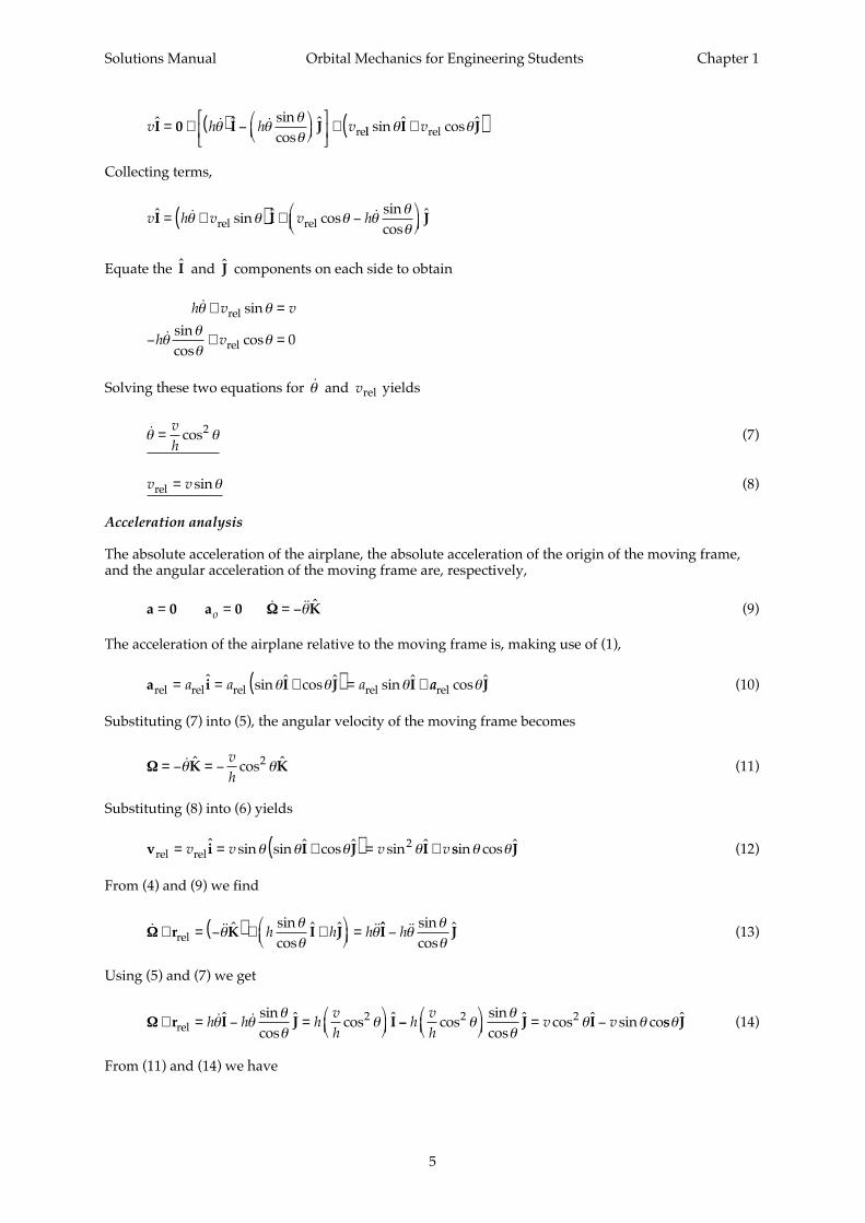
v h h vˆ ˆ sin
cosˆI 0 I J= + ( ) −
+θ θ
θθ rell relsin ˆ cos ˆθ θI J+( )v
Collecting terms,
v h v v hˆ sin ˆ cos
sincos
I I= +( ) + −
θ θ θ θθθrel rel
J
Equate the I and J components on each side to obtain
h v v
h v
θ θ
θθθ
θ
+ =
− + =
rel
rel
sin
sincos
cos 0
Solving these two equations for θ and vrel yields
θ θ=
vh
cos2 (7)
v vrel = sinθ (8)
Acceleration analysis
The absolute acceleration of the airplane, the absolute acceleration of the origin of the moving frame,and the angular acceleration of the moving frame are, respectively,
a 0 a 0 K= = = − ˆo ΩΩ θ (9)
The acceleration of the airplane relative to the moving frame is, making use of (1),
a i I J Irel rel rel rel= = +( ) = +a a aˆ sin ˆ cos ˆ sin ˆθ θ θ aarel cos ˆθJ (10)
Substituting (7) into (5), the angular velocity of the moving frame becomes
ΩΩ = − = −θ θˆ cos ˆK K
vh
2 (11)
Substituting (8) into (6) yields
v i I J Irel rel= = +( ) = +v v v vˆ sin sin ˆ cos ˆ sin ˆθ θ θ θ2 ssin cos ˆθ θJ (12)
From (4) and (9) we find
ΩΩ× = −( ) × +
=r K I Jrel θθθ
θˆ sincos
ˆ ˆh h h ˆ sincos
ˆI J− hθθθ
(13)
Using (5) and (7) we get
ΩΩ× = − =
r I J Irel h h hvh
θ θθθ
θˆ sincos
ˆ cos ˆ2 −−
= −hvh
v vcossincos
ˆ cos ˆ sin co2 2θθθ
θ θJ I ss ˆθJ (14)
From (11) and (14) we have
Solutions Manual Orbital Mechanics for Engineering Students Chapter 1
6
ΩΩ ΩΩ× ×( ) = −
−
r
I J K
rel
ˆ ˆ ˆ
cos
cos sin cos
0 0 2
2
vh
v v
θ
θ θ θ 00
23
24= − −
vh
vh
sin cos ˆ cos ˆθ θ θI J (15)
From (11) and (12),
2 2 0 0
0
22
2
ΩΩ× = − =v
I J K
rel
ˆ ˆ ˆ
cos
sin sin cos
vh
v v
θ
θ θ θ
vvh
vh
23
22 22sin cos ˆ sin cos ˆθ θ θ θI J− (16)
According to Equation 1.42, a a r r v a= + × + × ×( ) + × +o ΩΩ ΩΩ ΩΩ ΩΩrel rel rel rel2 . Substituting (9), (10),
(13), (15) and (16) yields
0 0 I J= + −
+ −h hvh
θ θθθ
θˆ sincos
ˆ sin cos2
332
4
23
22 2
θ θ
θ θ
ˆ cos ˆ
sin cos ˆ
I J
I
−
+ −
vh
vh
vh
ssin cos ˆ sin ˆ cos ˆ2 2θ θ θ θJ I J
+ +( )a arel rel
Collecting terms
0 = − + +
hvh
vh
aθ θ θ θ θ θ2
32
32sin cos sin cos sinrel
+ − − −
ˆ
sincos
cos sin co
I
hvh
vh
θθθ
θ θ2
42
22 ss cos ˆ2 θ θ+
arel J
or
0 I= + +
+ −h
vh
a hθ θ θ θ θ2
3sin cos sin ˆ srel
iincos
cos sin cos ˆθθ
θ θ θ− +( ) +
vh
a2
2 21 rel J
Equate the I and √J components on each side to obtain
h avh
h a
θ θ θ θ
θθθ
+ = −
− +
rel
r
sin sin cos
sincos
23
eel cos cos sinθ θ θ= +( )vh
22 21
Solving these two equations for ««θ and arel yields
θ θ θ θ= − =22
23
23v
ha
vhrelcos sin cos
Problem 1.6 From Equation 2.58b with z = 0 we have
a i j= − + − +2 22
2 2Ω Ω Ωy RyR
REE
Esin ˆ sin cos ˆ cosφ φ φ φφ
k (1)
where
Solutions Manual Orbital Mechanics for Engineering Students Chapter 1
7
R
y
E = ×
= °
=×
=
6378 10
30
1000 103600
27 78
3
3
m
m s
φ
.
Ω =
×= × −2
23 934 36007 2921 10 5π
.. rad s
Substituting these numbers into (1), we find
a i j k= − + − ( )0 0020256 0 014686 0 025557. ˆ . ˆ . ˆ m s
From F a= m , with m = 1000 kg , we obtain the net force on the car,
F i j k=-2.0256 Nˆ . ˆ . ˆ+ − ( )14 686 25 557
F Fxlateral N lb= = − = −2 0256 0 4554. . , that is
Flateral lb to the west= 0 4554.
The normal force N of the road on the car is given by N F mgz= + , so that
N = − + × =25 557 1000 9 81 9784. . N
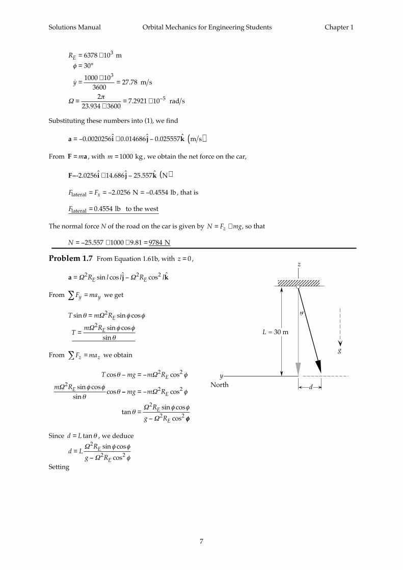
Problem 1.7 From Equation 1.61b, with z = 0 ,
a j k= −Ω Ω2 2 2R l l R lE Esin cos ˆ cos ˆ
From
F may y=∑ we get
T m R
Tm R
E
E
sin sin cos
sin cos
sin
θ φ φ
φ φ
θ
=
=
Ω
Ω
2
2
From F maz z=∑ we obtain
T mg m R
m R
E
E
cos cos
sin cos
sincos
θ φ
φ φ
θθ
− = − Ω
Ω
2 2
2−− = −
=−
mg m R
R
g R
E
E
E
Ω
Ω
Ω
2 2
2
2 2
cos
tansin cos
cos
φ
θφ φ
φφ
Since d L= tanθ , we deduce
d L
R
g RE
E
=−
Ω
Ω
2
2 2sin cos
cos
φ φ
φSetting
g
y
z
North d
L = 30 m
Solutions Manual Orbital Mechanics for Engineering Students Chapter 1
8
L
R
g
E
=
= × = ×
= °
=
=×
= × −
30
6378 1000 6 378 1029
9 812
23 9344 36007 2921 10
6
5
m
m
m s
rad s
2
.
.
..
φ
πΩ
yields
d = ( )44 1. mm to the south
Solutions Manual Orbital Mechanics for Engineering Students Chapter 2
9
d
m
m
Fg
c.m.
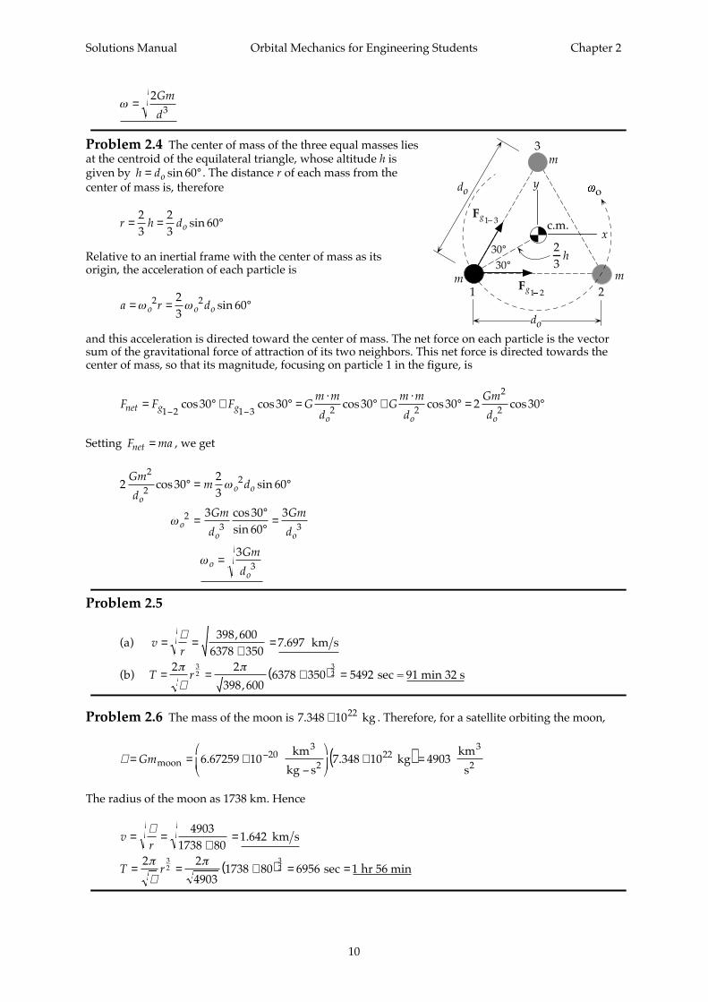
Problem 2.1
r I J K
r I J K
= + +
= + +( ) ⋅3 2 9
3 2 9 3
4 3 2
4 3 2
t t t
t t t t
ˆ ˆ ˆ
ˆ ˆ ˆ 44 3 2 8 6 4
7
2 9 9 4 81
36
ˆ ˆ ˆI J K
r
+ +( ) = + +
= =
t t t t t
rddt
t ++ +
+ +
12 162
9 4 81
5 3
8 6 4
t t
t t t
At t = 2 sec ,
« .r =
+ +
+ +=
4608 384 1296
2304 256 1296101 3 m s
r I J K
r I J K
=12t
12t
3
3
ˆ ˆ ˆ
ˆ ˆ ˆ
+ +
= + +(6 18
6 18
2
2
t t
t t )) ⋅ + +( ) = + +12t3ˆ ˆ ˆI J K6 18 144 36 3242 6 4 2t t t t t
At t = 2 sec ,
« .r = + + =9216 576 1296 105 3 m s
Problem 2.2
ˆ ˆ ˆ ˆ
ˆˆ ˆu u u u
uu ur r r r
rr r
ddt
ddt
⋅ = ⇒ ⋅( ) = ⇒ ⋅ +1 0 ⋅⋅ = ⇒ ⋅ =ddt
ddt
rr
rˆ ˆ
ˆuu
u0 0
Or,
ddt
ddt r
rddt
drdt
r
r r
rrˆ
ˆ
u rr
r r r=
=−
=−
2 2
uuu r r r r r
rrd
dt rr r
r r
rr
r⋅ = ⋅
−=
⋅−
ˆ2 2 2
But according to Equation 2.25, r r⋅ = rr . Hence ˆ
ˆu
ur
rddt
⋅ = 0
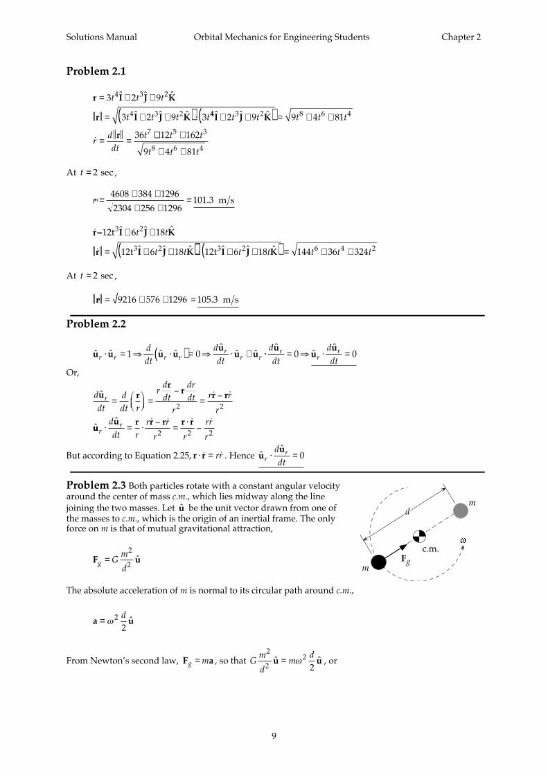
Problem 2.3 Both particles rotate with a constant angular velocityaround the center of mass c.m., which lies midway along the linejoining the two masses. Let u be the unit vector drawn from one ofthe masses to c.m., which is the origin of an inertial frame. The onlyforce on m is that of mutual gravitational attraction,
F ug G
m
d=
2
2ˆ
The absolute acceleration of m is normal to its circular path around c.m.,
a u= ω 2
2d ˆ
From Newton’s second law, F ag m= , so that
G
m
dm
d2
22
2ˆ ˆu u= ω , or
Solutions Manual Orbital Mechanics for Engineering Students Chapter 2
10
ω =
23
Gm
d
Problem 2.4 The center of mass of the three equal masses liesat the centroid of the equilateral triangle, whose altitude h isgiven by h do= °sin 60 . The distance r of each mass from thecenter of mass is, therefore
r h do= = °
23
23
60sin
Relative to an inertial frame with the center of mass as itsorigin, the acceleration of each particle is
a r do o o= = °ω ω2 22
360sin
and this acceleration is directed toward the center of mass. The net force on each particle is the vectorsum of the gravitational force of attraction of its two neighbors. This net force is directed towards thecenter of mass, so that its magnitude, focusing on particle 1 in the figure, is
F F F G
m m
dG
m m
d
Gm
dnet g g
o o o= ° + ° =
⋅° +
⋅° = °
− −1 2 1 3 2 2
2
230 30 30 30 2 30cos cos cos cos cos
Setting F manet = , we get
2 3023
60
3 3060
3
3
2
22
23 3
3
Gm
dm d
Gm
d
Gm
d
Gm
d
oo o
oo o
oo
cos sin
cossin
° = °
=°°
=
=
ω
ω
ω
Problem 2.5
(a) km s
(b) sec = 91 min 32 s
vr
T r
= =+
=
= = +( ) =
µ
π
µ
π
398 6006378 350
7 697
2 2
398 6006378 350 5492
32
32
,.
,
Problem 2.6 The mass of the moon is 7 348 1022. × kg . Therefore, for a satellite orbiting the moon,
µ = = ×
−
×( ) =−Gmmoon
3
2
3
2 km
kg s kg
km
s6 67259 10 7 348 10 490320 22. .
The radius of the moon as 1738 km. Hence
vr
T r
= =+
=
= = +( ) = =
µ
π
µ
π
49031738 80
1
2 2
49031738 80 6956 1
32
32
.642 km s
sec hr 56 min
x
y
m1 2
3
c.m.
Fg1 2
Fg1 3
30°
30°
do
do o
23
h
m
m
Solutions Manual Orbital Mechanics for Engineering Students Chapter 2
11
Problem 2.7 The time between successive crossings of the equator equals the period of the orbit.That is
dR
R zΩEarth Earth
Earth= +( )2 3 2π
µ/
where d = 3000 km is the distance between ground tracks, z is the altitude of the orbit,
REarth km= 6378 and ΩEarth rad s= ⋅( ) = × −2 23 934 3600 7 2921 10 5π . . . Thus
3000
7 2921 10 6378
2
398 6006378
53 2
./
×( )( )= +( )
−
πz
so that
z = 1440 7. km
Problem 2.8 From Example 2.3 we know that vGEO km s= 3 0747. . From Equation 2.82 we knowthat
v vesc = 2 circular. Hence ∆v v= −( ) = ⋅ =2 1 0 41421 3 0747 1 2736GEO km s. . . .
Problem 2.9
µ
µ
sun3 2
earth
earthsun
earth
esc
relative
km s
km
km s
km s km s
= ×
= ×
= =×
×=
= ⋅ =
= − =
1 3271 10
149 6 10
1 3271 10
149 6 1029 784
2 29 784 42 12142 121 29 784 12 337
11
6
11
6
.
.
.
..
. .. . .
r
vr
v
v
Problem 2.10
AT
abT
Aab
ab
3
31 0472
=
= =
π
π.
Problem 2.11
vh
e
vhr
h
he
r =
= =
+
⊥
µθ
µ θ
sin
cos
2 11
v v vr= + ⊥2 2
cos sin cos= +( ) + +
µθ θ θ
he e2 2 2 2 1
v
he e= + +
µθ2 2 1cos
Problem 2.12 For the ellipse, according to Problem 2.11,

Solutions Manual Orbital Mechanics for Engineering Students Chapter 2
12
v
he eellipse
22
22 2 1= + +( )µ
θcos
For the circle, at the point of intersection with the ellipse,
vr h
eh
ecircle2
2
2
211
1= =
+
= +( )µ µ
µ θ
µθ
cos
cos
Setting v vcircle ellipse
2 2= ,
µθ
µθ
2
2
2
221 2 1
he
he e+( ) = + +( )cos cos
yields e ecosθ = − 2 , or θ = −( )−cos 1 e .
Problem 2.13 From Equation 3.42
tan
sincos
γθθ
=+e
e1
From Problem 2.12 θ = −( )−cos 1 e . Hence
tan
sin cosγ =
−( )[ ]−
−e e
e
1
21
But sin cos− −( )[ ] = −1 21e e . Therefore,
tan γ =−
−=
−
e e
e
e
e
1
1 1
2
2 2
Problem 2.14(a)
e
r r
r r=
−
+=
−
+= ( )apogee perigee
apogee perigee ellipse
70 000 700070 000 7000
0 81818.
(b)
a
r r=
+= =
apogee perigee km
277 000
238 500
(c)
T a= = ( ) = ( )2 2
398 60038 500 75 1803 2 3 2π
µ
π/ / s 20.88 h
(d)
ε
µ= − = −
⋅= −
2398 600
2 38 5005 1766
a. km s2 2
(e) From Equation 3.62,
6378 100038 500 1 0 81818
1 0 818180 88615 27 607
2+ =
−( )+
= ⇒ = °
.. cos
cos . .θ
θ θ
Solutions Manual Orbital Mechanics for Engineering Students Chapter 2
13
(f) From Equation 3.40
h e r= +( ) = ⋅ +( ) ⋅ =µ 1 398 600 1 0 81818 7000 71 226perigee
2 km s.
Then
vhr
vh
er
⊥ = = =
= = ⋅ ⋅ ° =
71 2267378
9 6538
398 60071 226
0 81818 27 607 2 1218
.
sin . sin . .
km s
km sµ
θ
(g)
vh
r
vh
r
perigeeperigee
apogeeapogee
km s
km s
= = =
= = =
71 2267000
10 175
71 22670 000
1 0175
.
.
Problem 2.15
rperigee km= + =6378 250 6628
rapogee km= + =6378 300 6678
a
r r=
+=
+=
perigee apogee km
26628 6678
26653
T a= = ⋅ = ( )2 2
398 6006653 5400 53 2 3 2π
µ
π/ / . s 90.009 m
t
Tperigee to apogee m= =
245 005.
Problem 2.16(a)
e
r r
r r=
−
+=
+( ) − +( )+( ) + +( ) =
apogee perigee
apogee perigee
6378 1600 6378 6006378 1600 6378 600
0 066863.
(b)
h e r s= +( ) = ⋅ +( ) ⋅ +( ) =µ 1 398 600 1 0 066863 6378 600 54 474perigee
2 km.
vh
r
vh
r
perigeeperigee
apogeeapogee
km s
.8280 km s
= =+
=
= =+
=
54 4746378 600
7 8065
54 4746378 1600
6
.
(c)
Th
e=
−
=
−
=
2
1
2
398 600
54 474
1 0 0668636435 62 2
3
2 2
3π
µ
π
.. s = 107.26 m
Problem 2.17
h r v= = +( ) ⋅ =perigee perigee
2 km s6378 1270 9 68 832
r
heperigee =
+
2
21
1µ
Solutions Manual Orbital Mechanics for Engineering Students Chapter 2
14
6378 1270
68 832
398 600
11
0 554162
2+ =+
⇒ =e
e .
tan
sincos
. sin. cos
. .γθθ
γ=+
=⋅ °
+ °= ⇒ = °
ee1
0 55416 1001 0 55416 100
0 60385 31 13
z R
he
+ =+earth
2 11µ θcos
z z+ =
+ °⇒ =6378
68 832398 600
11 0 55416 100
6773 82
. cos . km
h r v
rh
e
ee
ee
z Rh
e
z
= = +( ) ⋅ =
=+
+ =+
⇒ =
=+
=⋅ °
+ °= ⇒ = °
+ =+
+ =
perigee perigee2
perigee
earth
km s6378 1270 9 68 832
11
6378 127068 832
398 600
11
0 55416
10 55416 100
1 0 55416 1000 60385 31 13
11
6378
2
2
2
2
2
µ
γθθ
γ
µ θ
.
tansin
cos. sin
. cos. .
cos
6868 832398 600
11 0 55416 100
6773 82
+ °⇒ =
. cos .z km
Problem 2.18
v v
v v
h rv
r = = ⋅ ° =
= = ⋅ ° =
∴ = = +( ) ⋅ =
⊥
⊥
sin . sin .cos . cos .
.
γ
γ
9 2 10 1 59769 2 10 9 0602
6378 640 9 0602 63 585
km s km s
km s2
rh
e
e
e
vh
e
e
e
r
=+
+ =+
=
=
=
=
= = = ⇒ = °
2
2
11
6378 64063 585398 600
11
0 445 29
1 5976398 60063 585
0 254 840 254 840 445 29
0 572 31 29 783
µ θ
θ
θ
µθ
θ
θ
θθθ
θ
cos
coscos .
sin
. sin
sin .
tansincos
.
.. .
e e
Th
e
sin . . .
.
29 783 0 254 84 0 51306
2
1
2
398 600
63 585
1 0 5130616 0752 2
3
2 2
3
° = ⇒ =
=−
=
−
=
π
µ
π s = 4.4654 h
Solutions Manual Orbital Mechanics for Engineering Students Chapter 2
15
Problem 2.19
a
r r=
+=
+( ) + +( )=
perigee apogee km
26378 250 6378 42 000
227 503
T a= = =
2 2
398 60027 503 45 3923 2 3 2π
µ
π/ / s = 12.61 h
e
r r
r r=
−
−=
+( ) − +( )
+( ) + +( ) =apogee perigee
apogee perigee
6378 42 000 6378 2506378 42 000 6378 250
0 75901.
h e r= +( ) = ⋅ +( ) ⋅ +( ) =µ 1 398 600 1 0 75901 6378 250 68 170perigee
2 km s.
v
hrperigeeperigee
km s= =+
=68 170
6378 25010 285.
Problem 2.20
h r v
rh
e
ee
rh
e
z
ar r
= = +( ) ⋅ =
=+
=+
⇒ =
=−
=−
=
= − =
=+
=( ) + ( )
=
perigee perigee
perigee
apogee
apogee
perigee apogee
km s
km
km
6378 640 8 56 144
11
701856 144398 600
11
0 126 82
11
56 144398 600
11 0 126 82
9056 6
9056 6 6378 2678 6
27018 9056 6
28037
2
2
2 2
µ
µ
.
..
. .
...
./ /
3
2 2
398 6008037 3 71713 2 3 2
km
s = 1.992 hT a= = =π
µ
π
Problem 2.21
T a
a a
=
⋅ = ⇒ =
2
2 36002
398 6008059
3 2
3 2
π
µ
π
/
/ km
Using the energy equation
v
r a
rr
z
perigee
perigee
perigeeperigee
perigee
km
km
2
2
2 2
82
398 600 398 6002 8059
7026 2
7026 2 6378 648 25
− = −
− = −⋅
⇒ =
= − =
µ µ
.
. .
Solutions Manual Orbital Mechanics for Engineering Students Chapter 2
16
Problem 2.22
T a=
2 3 2π
µ/
90 60
26652 63 2⋅ = ⇒ =
π
µa a/ . km
r r aperigee apogee+ = 2
6378 + 150 kmapogee apogee( ) + = ⋅ ⇒ =r r2 6652 6 6777 1. .
e
r r
r r=
−
+=
−+
=apogee perigee
apogee perigee
6777 1 65286777 1 6528
0 018 723..
.
Problem 2.23
(a)
vr
v v v
esc
perigee esc
km s
km s
= =+
=
= − = − =∞
2 2398 600
6378 30010 926
15 10 926 10 2772 2 2 2
µ.
. .
(b)
h r v= = ⋅ =perigee perigee
2 km s6678 15 100 170
r
heperigee =
+
2 11µ
6678
100 170398 600
11
2 76962
=+
⇒ =e
e .
r
he
=+
=+ °
=2 21
1100 170398 600
11 2 7696 100
48 497µ θcos . cos
km s
(c)
vh
e
vhr
r = = ⋅ ⋅ ° =
= = =⊥
µθsin . sin .
.
398 600100 170
2 7696 100 10 853
100 17048 497
2 0655
km s
km s
Problem 2.24
(a) From Equation 3.47
ε
µ= − = − =
vr
2 2
22 23
2398 600402 000
1 4949.
. km s2 2
From Equation 3.50
h e e
h e
22
22
2
2 2 10
12
112
398 6001 4949
1
5 3141 1 10
= − −( ) = − −( )
= −( )×
µε .
.
From the orbit equation

Solutions Manual Orbital Mechanics for Engineering Students Chapter 2
17
h r e e
h e
2
2 10
1 398 600 402 000 1 150
16 024 13 877 10
= +( ) = ⋅ ⋅ + °( )
= −( ) ×
µ θcos cos
. .
Equating the two expressions for h2 ,
5 3141 1 10 16 024 13 877 102 10 10. . .e e−( )× = −( ) ×
yields
e e2 22 6113 4 0153 0+ − =. .
which has the positive root
e = 1 086.
(b) Using this value of the eccentricity we find
h2 10 916 024 13 877 1 086 10 9 5334 10= − ⋅( ) × = ×. . . . km s4 2
so that
rh
e
z
perigee
perigee
km
km
=+
=×
+=
= − =
2 911
9 5334 10398 600
11 1 086
11 466
11 466 6378 5087 6µ
..
.
(c)
v
hrperigeeperigee
km s= =×
=9 5334 10
11 4668 5158
9..
Problem 2.25 From the energy equation
v v v
vr
v
rv
∞
∞ ∞
∞
+ =
+ = ( )
=
2 2 2
2 2
2
21 1
9 5238
esc
µ
µ
.
.
Substituting Equation 3.105
r
he
h
e=
−
=−
9 5238
1
9 52381
122
2
2. .µ
µ µ
Using Equation 3.40
r r e
e
r
e= +( )[ ]
−=
−9 5238 1
1
19 5238
12. .perigeeperigee
Problem 2.26
v
he∞ = − = − =
µ 2 21398 600105 000
3 1 10 737. km s
Solutions Manual Orbital Mechanics for Engineering Students Chapter 2
18
Problem 2.27(a)
r
he1
2
1
11
=+µ θcos
6378 1700
398 6001
1 130
2+ =
+ °h
e cos
h e2 93 2199 2 0697 10= −( ) ×. .
r
he2
2
2
11
=+µ θcos
6378 500
398 6001
1 50
2+ =
+ °h
e cos
h e2 92 7416 1 7622 10= +( ) ×. .
3 2199 2 0697 10 2 7416 1 7622 103 832 0 478 32
0 124 82
9 9. . . .. .
.
−( ) × = +( ) ×
=
=
e e
e
e
(b)
h2 9 92 7416 1 7622 0 124 82 10 2 9615 10= + ⋅( )× = ×. . . . km s4 2
r
heperigee km=
+=
×+
=2 91
12 9615 10
398 6001
1 0 124 826605 4
µ.
..
zperigee km= − =6605 4 6378 227 35. .
(c) From Equation 3.63,
a
r
e=
−=
−=
perigee km
16605 4
1 0 124 827547 5
..
.
Problem 2.28
(a)
vv
v vrr
⊥⊥= = ° = ⇒ =tan tan . .γ 15 0 26795 0 26795
v v vr2 2 2= + ⊥
7 0 267952 2 2= ( ) +⊥ ⊥. v v
∴ =
=⊥v
vr
6 76151 8117
.
. km s km s
h rv= = ⋅ =⊥ 9000 6 7615 60 853. km s2
vh
e
e
e
r =
=3
=
µθ
θ
θ
sin
. sin
sin .
1 811798 60060 853
0 27659

Solutions Manual Orbital Mechanics for Engineering Students Chapter 2
19
rh
e
e
e
ee
=+
=+
=
= = = ⇒ = °
2
2
11
900060 853398 600
11
0 032259
0 276590 032259
8 574 83 348
µ θ
θ
θ
θθθ
θ
cos
coscos .
tansincos
..
. .
(b)
e ecos . . .83 348 0 032259 0 27847° = ⇒ =
Problem 2.29 From Equation 3.50,
εµ
= − −( )
− = − −( ) ⇒ =
12
1
2012
398 600
60 0001 0 30605
2
22
2
22
he
e e .
rh
e
z
perigee
perigee
km
km
=+
=+
=
= − =
2 211
60 000398 600
11 0 30605
6915 2
6915 2 6378 537 21µ .
.
. .
rh
e
z
apogee
apogee
km
636.8 km
=−
=−
=
= − =
2 211
60 000398 600
11 0 30605
13 015
13 015 6378 6µ .
Problem 2.30(a)
v v⊥ = = ⋅ ° =cos . cos .γ 8 85 6 8 8015 km s
h rv= = +( ) ⋅ =⊥ 6378 550 8 8015 60 977. km s2
r
he
=+
2 11µ θcos
6928
60 977398 600
11
0 346442
=+
⇒ =e
ecos
cos .θ
θ
v vr = = ⋅ ° =sin . sin .γ 8 85 6 0 92508 km s
v
her =
µθsin
0 92508
398 60060 977
0 14152. sin sin .= ⇒ =e eθ θ
∴ = = ⇒ = °tan
sincos
. .θθθ
θee
0 40849 22 22
e esin . . .22 22 0 14152 0 37423° = ⇒ =
(b)
Th
e=
−
=
−
=
2
1
2
398 600
60 977
1 0 3742311 2432 2
3
2 2
3π
µ
π
. s = 187.39 m
Solutions Manual Orbital Mechanics for Engineering Students Chapter 2
20
Problem 2.31
v v
h rv
rh
e
ee
⊥
⊥
= = ⋅ ° =
= = ( ) ⋅ =
=+
=+
⇒ =
cos cos .
.
cos
cos cos .
γ
µ θ
θθ
10 30 8 6603
10 000 8 6603 86 603
11
10 00086 603398 600
11
0 88159
2
2
km s
km s2
v v
vh
e
e e
r
r
= = ⋅ ° =
=
= ⇒ =
sin sin
sin
sin sin .
γ
µθ
θ θ
10 30 5
5398 60086 603
1 0863
km s
∴ = = ⇒ = °tan
sincos
. .θθθ
θee
1 2323 50 94
Problem 2.32
v v
h rv
rh
e
ee
⊥
⊥
= = ⋅ ° =
= = ( ) ⋅ =
=+
=+
⇒ =
cos cos .
.
cos
cos cos .
γ
µ θ
θθ
10 20 9 3969
15 000 9 3969 140 950
11
15 000140 950398 600
11
2 323
2
2
km s
km s2
v v
vh
e
e e
r
r
= = ⋅ ° =
=
= ⇒ =
sin sin .
sin
. sin sin .
γ
µθ
θ θ
10 20 3 4202
3 4202398 600140 950
1 2095
km s
∴ = = ⇒ = °tan
sincos
. .θθθ
θee
0 52065 27 504
Problem 2.33 Using the orbit equation r
he
=+
2 11µ θcos
we find
he e
he e
e e
e e
2
2
10 000 1 30 10 000 8660 3
30 000 1 105 30 000 7764 6
10 000 8660 3 30 000 7764 616 425 20 000 1 2177
µ
µ
= + °( ) = +
= + °( ) = −
∴ + = −
= ⇒ =
cos .
cos .
. . .
Problem 2.34
v
r1398 600
6378 5007 6127= =
+=
µ. km s
Solutions Manual Orbital Mechanics for Engineering Students Chapter 2
21
v v
v2 1
12
11 419= + = . km s
v vr
∞ −∞
= −2
22
2 2µ µ
vv∞∞= − = ⇒ =
2 2
211 419
2398 600
68787 2441 3 8062
.. . km s
Problem 2.35
vr
v v
h r v
rh
e
ee
rh
e
z
1
1
2
2
2 2
398 6006378 320
7 7143
0 5 8 2143
6698 8 2143 55 019
11
669855 019398 600
11
0 13383
11
55 019398 600
11 0 13383
8767 8
8767 8
= =+
=
= + =
= = ⋅ =
=+
=+
⇒ =
=−
=−
=
=
µ
µ
µ
.
. .
.
.
..
.
km s
km s
km
perigee
perigee perigee
perigee
apogee
apogee −− =6378 2389 8. km
Problem 2.36
v
r=
µ
perigee
v v v
rperigeeperigee
= + = +( )α αµ
1
h r v r
rr= = +( ) +( )perigee perigee perigee
perigeeperigee =1 1α
µα µ
r
he
r
eperigeeperigee
=+
=+( )
+
2 21
1
1 11µ
α µ
µ
∴ + = +( )
+ = + + ⇒ = +( )
1 1
1 1 2 2
2
2
e
e e
α
α α α α
Problem 2.37(a)
v
r1398 600
6378 4007 6686= =
+=
µ. km s
v v⊥ = + =2 1 0 24 7 9086. . km s
h rv2 2 6778 7 9086 53 605= = ⋅ =⊥ . km s2
r
he
=+
22 1
1µ
6778
53 605398 600
11
0 0635722
=+
⇒ =e
e .
zperigee km
2400=
Solutions Manual Orbital Mechanics for Engineering Students Chapter 2
22
6378 + kmapogee apogeez
he
z2
22 2
2
11
53 605398 600
11 0 063572
1320 3=−
=−
⇒ =µ .
.
(b)
vr
h rv
vh
e
e e
rh
e
ee
r
⊥
⊥
= =+
=
= = ⋅ =
=
= ⇒ =
=+
=+
⇒ = ⇒ =
2
2 2
22
2
2 2
22
22
22
398 6006378 400
7 6686
6778 7 6686 51 978
0 24398 60051 978
0 031296
11
677851 978398 600
11
0 90
µ
µθ
θ θ
µ θ
θθ θ
.
.
sin
. sin sin .
cos
cos cos
km s
km s2
°° ≠( )
° = ⇒ =
+ =+
=+
⇒ =
=−
=−
⇒ =
since cannot be zero if
km
6378 + km
perigee perigee
apogee apogee
e v
e e
zh
ez
zh
ez
r 0
90 0 031296 0 031296
63781
151 978398 600
11 0 031296
196 49
11
51 978398 600
11 0 031296
631 3
2 2
22
2 2
2
22
2 2
2
sin . .
. .
. .
µ
µ
Problem 2.38 In Figure 3.30
m m
m m
r
130
24
126
1 989 10
5 974 10
149 6 10
= = ×
= = ×
= ×
sun
2 earth
kg
kg
km
.
.
.
From Equation 3.169
π2 =
+= × −m
m m2
1 2
63 0035 10.
Substitute π2 into Equation 3.195,
f ξπ
ξ πξ π
π
ξ πξ π ξ( ) =
−
++( ) +
+ −+ −( ) −1
112
23 2
2
23 2
The graph of f ξ( ) is similar to Figure 3.33, with the two crossings on the right much more closelyspaced. Zeroing in on the regions where f ξ( ) = 0 , with the aid of a computer, reveals
ξ
ξ
ξ
1
2
3
0 990 026 61 010 034
1 000 001
=
=
= −
.
..
Then,
x r
x r
x r
1
2
3
km
km
km
= = ×
= = ×
= = − ×
ξ
ξ
ξ
1 126
2 126
3 126
148 108 10
151 101 10
149 600 10
.
.
.
Solutions Manual Orbital Mechanics for Engineering Students Chapter 2
23
These are the locations of L1, L2 and L3 relative to the center of mass of the sun-earth system(essentially the center of the sun).
Solutions Manual Orbital Mechanics for Engineering Students Chapter 2
24
Solutions Manual Orbital Mechanics for Engineering Students Chapter 3
25
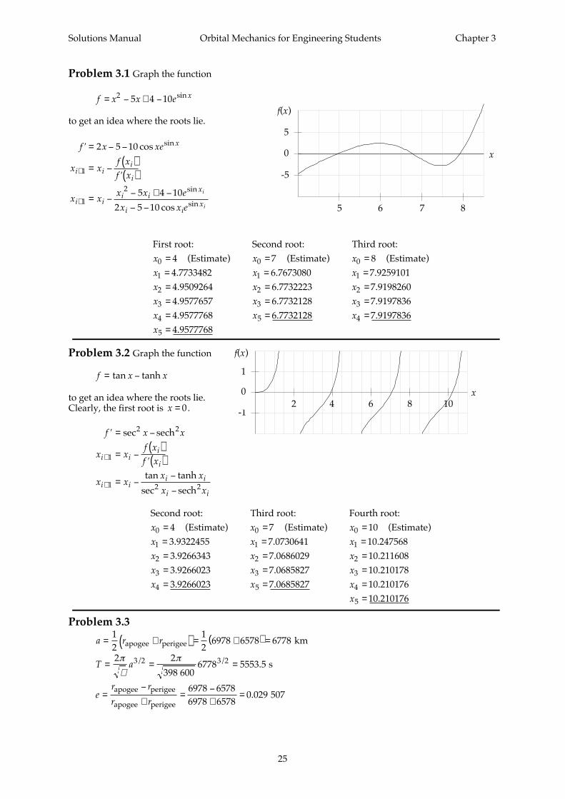
Problem 3.1 Graph the function
f x x e x= − + −2 5 4 10 sin
to get an idea where the roots lie.
First root: (Estimate)
Second root: (Estimate)
Third root: (Estimate)x
x
x
x
x
x
x
x
x
x
x
x
x
x
x
x
0
1
2
3
4
5
0
1
2
3
5
0
1
2
3
4
44 77334824 95092644 95776574 95777684 9577768
76 76730806 77322236 77321286 7732128
87 92591017 91982607 91978367 9197836
=
=
=
=
=
=
=
=
=
=
=
=
=
=
=
=
.....
....
....
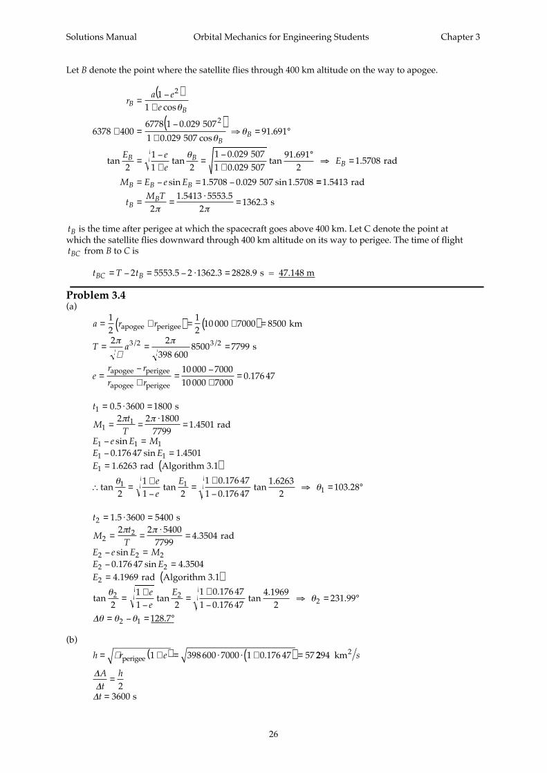
Problem 3.2 Graph the function
f x x= −tan tanh
to get an idea where the roots lie.Clearly, the first root is x = 0.
′ = −
= −( )′( )
= −−
−
+
+
f x x
x xf xf x
x xx x
x x
i ii
i
i ii i
i i
sec
tan tanh
sec
2 2
1
1 2 2
sech
sech
Second root: (Estimate)
3.93224553.92663433.92660233.9266023
Third root: (Estimate)
7.07306417.06860297.06858277.0685827
Fourth root: (Estimate)
10.24756810.21160810.21017810.21017610.210176
x
x
x
x
x
x
x
x
x
x
x
x
x
x
x
x
0
1
2
3
4
0
1
2
3
5
0
1
2
3
4
5
4 7 10=
=
=
=
=
=
=
=
=
=
=
=
=
=
=
=
Problem 3.3
a r r= +( ) = +( ) =
12
12
6978 6578 6778apogee perigee km
T a= = =
2 2
398 6006778 5553 53 2 3 2π
µ
π/ / . s
e
r r
r r=
−
+=
−+
=apogee perigee
apogee perigee
6978 65786978 6578
0 029 507.
f(x)
5 6 7 8
-5
0
5
x
2 4 6 8 10-1
0
1
x
f(x)
′ = − −
= −( )′( )
= −− + −
− −
+
+
f x xe
x xf x
f x
x xx x e
x x e
x
i ii
i
i ii i
x
i ix
i
i
2 5 10
5 4 10
2 5 10
1
1
2
cos
cos
sin
sin
sin
Solutions Manual Orbital Mechanics for Engineering Students Chapter 3
26
Let B denote the point where the satellite flies through 400 km altitude on the way to apogee.
ra e
e
E ee
E
M E e E
BB
BB
B BB
B B B
=−( )
+
+ =−( )
+⇒ = °
=−+
=−
+°
⇒ =
= − = −
11
6378 4006778 1 0 029 507
1 0 029 50791 691
211 2
1 0 029 5071 0 029 507
91 6912
1 5708
1 5708 0 029 507 1 5708
2
2
cos
.
. cos.
tan tan..
tan.
.
sin . . sin .
θ
θθ
θ rad
==
= =⋅
=
1 5413
21 5413 5553 5
21362 3
.. .
.
rad
stM T
BBπ π
tB is the time after perigee at which the spacecraft goes above 400 km. Let C denote the point atwhich the satellite flies downward through 400 km altitude on its way to perigee. The time of flight
tBC from B to C is
t T tBC B= − = − ⋅ =2 5553 5 2 1362 3 2828 9. . . s = 47.148 m
Problem 3.4(a)
a r r= +( ) = +( ) =
12
12
10 000 7000 8500apogee perigee km
T a= = =
2 2
398 6008500 77993 2 3 2π
µ
π/ / s
e
r r
r r=
−
+=
−
+=
apogee perigee
apogee perigee
10 000 700010 000 7000
0 176 47.
t1 0 5 3600 1800= ⋅ =. s
M
tT1
12 2 18007799
1 4501= =⋅
=π π
. rad
E e E M1 1 1− =sin
E E1 10 176 47 1 4501− =. sin .
E1 1 6263= ( ). rad Algorithm 3.1
∴ =
+−
=+
−⇒ = °tan tan
.
.tan
. .
θθ1 1
1211 2
1 0 176 471 0 176 47
1 62632
103 28ee
E
t2 1 5 3600 5400= ⋅ =. s
M
tT2
22 2 54007799
4 3504= =⋅
=π π
. rad
E e E M2 2 2− =sin
E E2 20 176 47 4 3504− =. sin .
E2 4 1969= ( ). rad Algorithm 3.1
tan tan
.
.tan
. .
θθ2 2
2211 2
1 0 176 471 0 176 47
4 19692
231 99=+−
=+
−⇒ = °
ee
E
∆θ θ θ= − = °2 1 128 7.
(b)
h r e= +( ) = ⋅ ⋅ +( ) =µ perigee 1 398 600 7000 1 0 176 47 57. 2294 km2 s
∆∆At
h=
2 ∆t = 3600 s
Solutions Manual Orbital Mechanics for Engineering Students Chapter 3
27
∴ = = ⋅ = ×∆ ∆A h t
12
12
57 294 3600 103 13 106. km2
Problem 3.5(a)
T a
a a
a r r
r r
er r
r r
MtT
E e
=
⋅ = ⇒ =
= +( )
= +( ) ⇒ =
=−
+=
−
+=
= = =
−
2
15 743 36002
398 60031890
12
3189012
12756 51024
51024 1275651024 12756
0 6000
2 210
15 7433 9911
3 2
3 2
π
µ
π
π π
/
/.
.
..
sin
km
km
rad
perigee apogee
apogee apogee
apogee perigee
apogee perigee
EE M
E E
E
ee
E
ra e
e
=
− =
=
=+−
=+−
⇒ = °
=−( )
+=
−( )+ °
=
0 6 3 99113 6823
11 2
1 0 61 0 6
3 68232
195 78
11
31890 1 0 61 0 6 195 78
48 9242 2
. sin ..
tan..
tan.
.
cos.
. cos .
rad (Algorithm 3.1)
tan2
km
θθ
θ
(b)
vr a
vv
2
22 2
2398 60048 924
398 6002 31890
2 0019
− = −
− = −⋅
⇒ =
µ µ
. km s
(c)
h a e
vh
er
= −( ) = ⋅ ⋅ −( ) =
= = ⋅ ⋅ ° = −
µ
µθ
1 398 600 31890 1 0 6 90196
398 60090196
0 6 195 78 0 720 97
2 2.
sin . sin . .
km s
km s
2
Problem 3.6(a)
M E e EPB = − sin
22 2
π π πtT
ePB = − sin
t e
TPB = −
ππ2 2
t t
eTDPB PB= = −
2
12 π
(b)
t
TtBA PB= −
2
t
Te
T eTBA = − −
= +
2 2 2
14 2
ππ π
Solutions Manual Orbital Mechanics for Engineering Students Chapter 3
28
t t
eTBAD BA= = +
2
12 π
Problem 3.7
tan tan..
tan . .
sin . . sin . ..
.
E ee
E
M E e E
tM
T T T
B BB
B B B
BB
211 2
1 0 31 0 3 4
0 733 80 1 2661
1 2661 0 6 1 2661 0 97992
20 97992
20 48996
=−+
=−+
= ⇒ =
= − = − =
= = =
θ π
π π
rad
rad
Problem 3.8
ar r
er r
r r
T a
E ee
E
=+
=+
=
=−
+=
−
+=
= = =
=−+
°
=
−+
°( ) = ⇒= °
apogee perigee
apogee perigee
apogee perigee
km
s
214 000 7000
210 500
14 000 700014 000 7000
0 33333
2 2
398 60010 500 10708
211
602
1 0 333331 0 33333
30 0 40825
3 2 3 2
60
.
tan tan..
tan .
/ /π
µ
π
θθ == °
= °
= °= °
=
= − ( ) =
= = =
60
60
6060
0 77519
0 77519 0 33333 0 77519 0 54191
20 54191
210708 923 51
.
. . sin . ..
.
rad
rad
s
M
tM
T
θ
θθπ π
t t
MtT
θ θ
θθπ π
= + ⋅ =
= = =
= °60 30 60 2723 5
2 22723 510708
1 5981
..
.
s
rad
E e E M
E E E
ee
E
θ θ θ
θ θ θ
θθθ
− =
− = ⇒ =
=+−
=+−
⇒ = °
sin. sin . .
tan..
tan.
.
0 33333 1 5981 1 9122
11 2
1 0 333331 0 33333
1 91222
126 95
rad (Algorithm 3.1)
tan2
Problem 3.9
a b ccos sinθ θ+ =
cos sinθ θ+ =
ba
ca
ba≡ =tan
sincos
φφφ
cos
sincos
sinθφφ
θ+ =ca
cos cos sin sin cosθ φ θ φ φ+ =
ca
cos cosθ φ φ−( ) =
ca
θ φ φ− = ±
−cos cos1 ca
θ φ φ= ±
−cos cos1 ca
Solutions Manual Orbital Mechanics for Engineering Students Chapter 3
29
Problem 3.10
M E e E
tT
e
te
T e
B B B
B
B
= −
= −
=−
= −( )
sin
sin
sin. .
22 2
2 22
0 25 0 15915
ππ π
π π
πΤ
Problem 3.11
rh
e
rh
e
rr e
e
rr
E ee
E
B
B B
B B
=+
=+
⇒ =+( )
+
=+( )
+
= − ⇒ = °
=−+
=−+
°⇒
2
2
11
11
1
1
21 0 5
1 0 50 5 120
211 2
1 0 51 5
1202
µ θ
µ
θ
θ
θ θ
θ
cos
cos
.
. coscos .
tan tan..
tan
perigee
perigee
perigeeperigee
BB
B B B
BB
M E e E
tM
T T T
=
= − = − =
= = =
π
π π
π π
2
20 5
21 0708
21 0708
20 17042
rad
radsin . sin .
..
Problem 3.12 From Example 3.3 we have
e
T
c
=
=
=
0 246498679 1143 36
..
. s
θ
Thus
tan tan..
tan.
.
sin . . sin . ..
. .
E ee
E
M E e E
tM
T
c cc
c c c
cc
211 2
1 0 246491 0 24649
143 362
2 3364
2 3364 0 24649 2 3364 2 1587
22 1587
28679 1 2981 8
=−+
=−+
°⇒ =
= − = − ⋅ =
= = ⋅ =
θ
π π
rad
rad
s
Problem 3.13
rSOI km= 925000
r
r e
e=
+( )
+perigee 1
1 cosθ
925000
6378 500 1 11 1
170 11=+( ) +( )
+ ⋅⇒ = °
cos .
θθ
Mp tan tan tan
.tan
..= + =
°+
°=
12 2
16 2
12
170 112
16
170 112
262 823 3θ θ
r
hh rperigee perigee
2 km s= ⇒ = = ⋅ ⋅ =2
22 2 398 600 6878 74 048
µµ
Solutions Manual Orbital Mechanics for Engineering Students Chapter 3
30
t
hMp= = ⋅ =
3 374 048398 600
262 82 671630µ
. s = 7d 18h 34m
Problem 3.14(a)
h r e
M
th
M
t
p
p
= +( ) = ⋅ ⋅ +( ) =
) =°
+°
=
= ) = =
= ⋅ = =
= °
= ° = °
− ° °
µ
µ
θ
θ θ
perigee2
to +90
km s
s
s h
1 398 600 7500 1 1 77 324
12
902
16
902
0 66667
77 324
389 6000 66667 1939 9
2 1939 9 3879 8 1 0777
903
90
3
2 90
3
2
90
tan tan .
. .
. . .
(b)
Mt
h
M M M M
p
p p p p
= =⋅ ⋅( )
=
= + ( ) +
− + ( ) +
= ⋅ + ⋅( ) +[ ] − ⋅ + ⋅( ) +
−
µ
θ
θ
2
3
3
3
21 3
21 3
21 3
2
398 600 24 3600
77 32429 692
23 3 1 3 3 1
23 29 692 3 29 692 1 3 29 692 3 29 692 1
.
tan
tan . . . .
/ /
/ [[ ] =
= °
=+
=+ °
=
−1 3
2 2
5 4492
159 2
11
77 324398 600
11 159 2
230 200
/.
.
cos cos .
θ
µ θr
h km
Problem 3.15(a)
v
rperigeeperigee
km s= =⋅
=1 12
1 12 398 600
750011 341. . .
µ
h r v= = ⋅ =perigee perigee
2 km s7500 11 341 85056.
r
heperigee =
+
2 11µ
7500
85056398 600
11
1 42002
=+
⇒ =e
e .
tanh tan
.
.tan .
F ee
F90902
11
902
1 42 11 42 1
902
0 887 14°°=
−+
°=
−+
°⇒ =
M e F Fh ) = − = ⋅ − =° ° °90 90 90 1 42 0 88714 0 88714 0 544 46sinh . sinh . . .
M
he th ) = −( )
° °90
2
32 3 2
901µ /
0 544 46
398 600
850561 42 1 2057 9
2
32 3 2
90 90. . ./
= −( ) ⇒ =° °t t s
t t-90 to 90 s = 1.1433 h° ° °= =2 4115 790 .
(b)
M
he th = −( ) = −( ) ⋅ ⋅ =
µ2
32 3 2 2
32 3 2
1398 600
850561 42 1 24 3600 22 859
/ /. .
e F F Mhsinh − =
1 42 22 859 3 6196. sinh . . F F F− = ⇒ = ( )Algorithm 3.2
Solutions Manual Orbital Mechanics for Engineering Students Chapter 3
31
tan tanh
.
.tanh
. .
θθ
211 2
1 42 11 42 1
3 61962
132 55=+−
=+−
⇒ = °ee
F
r
he
=+
=+ ⋅ °
=2 21
185056398 600
11 1 42 132 55
455 660µ θcos . cos .
km
Problem 3.16
h r v
rh
e
eh
r
ah
e
= = +( ) ⋅ =
=+
= − =⋅
− = ( )
=−
=−
=
perigee perigee2
perigee
perigee
km s
hyperbola
km
6378 300 11 5 76 797
11
176 797
398 600 68781 1 2157
1
1
76 797398 600
1
1 2157 130 964
2
2 2
2
2
2
2
.
.
.
µ
µ
µ
At 6 AM:
vr a
rr
2
22 2
102
398 600 398 6002 30 964
9149 9
− =
− =⋅
⇒ =
µ µ
. km
rh
e
towards
F ee
F
M e F Fh
=+
=+
⇒ = − ° ( )
=−+
=−+
− °= − ⇒ = −
= − = −( ) − −
2
2
11
9149 976 797398 600
11 1 2157
59 494
211 2
1 2157 11 2157 1
59 4942
0 10384 0 360 45
1 2157 0 360 45 0
µ θ
θθ
θ
cos
.. cos
.
tanh tan..
tan.
. .
sinh . sinh .
flying earth
.. .
. . .
/
/
360 45 0 087 287
1
0 087 287398 600
76 7971 2157 1 753 3
2
32 3 2
2
32 3 2
( ) = −
= −( )
− = −( ) ⇒ = − ( )
Mh
e t
t t until
hµ
s negative means time perigee
At 11 AM:
t
Mh
e t
e F F M
F F F
ee
F
h
h
= ⋅ − − = ( )
= −( ) = −( ) ⋅ =
− =
− = ⇒ = ( )
=+−
=+
5 3600 753 3 17 247
1398 600
76 7971 2157 1 17 247 1 9984
1 2157 1 9984 1 8760
211 2
1 2157 1
2
32 3 2
2
2
32 3 2
.
. .
sinh
. sinh . .
tanh tan.
/ /
s time perigee at 11 AM
Algorithm 3.2
since
µ
θ11 2157 1
1 87602
133 96
11
76 797398 600
11 1 2157 133 96
94771
6378 88 393
2 2.
tan.
.
cos . cos .
−⇒ = °
=+
=+ ⋅ °
=
= − =
θ
µ θr
he
z r
km
km
Solutions Manual Orbital Mechanics for Engineering Students Chapter 3
32
Problem 3.17
v v
h rv
rh
e
ee
v v
vh
e
r
r
⊥
⊥
= = ⋅ − °( ) =
= = +( ) ⋅ =
=+
=+
⇒ =
= = ⋅ − °( ) = −
=
−
cos cos .
.
cos
cos cos .
sin sin .
sin
.
γ
µ θ
θθ
γ
µθ
8 65 3 3809
37 000 6378 3 3809 146 660
11
43 378146 660398 600
11
0 24397
8 65 7 2505
7 2505
2
2
km s
km s
km s
2
== ⇒ = −
= =−
= − ⇒ = − °
− °( ) = − ⇒ = ( )
=+
=+
= ( )
398 600146 660
2 6677
2 66770 24397
10 935 84 775
84 775 2 6677 2 6788
11
146 660398 600
11 2 6788
14 6682 2
e e
ee
e e
rh
e
sin sin .
tansincos
..
. .
sin . . .
.
θ θ
θθθ
θ
µ
hyperbola
km no impactperigee
tanh tan..
tan.
.
sinh . sinh . . .
. .
/
/
F ee
F
M e F F
Mh
e t
h
h
211 2
2 6788 12 6788 1
84 7752
1 4389
2 6788 1 4389 1 4389 3 8906
1
3 8906398 600
46 6602 6788 1
2
32 3 2
2
32 3 2
=−+
=−+
− °
⇒ = −
= − = −( ) − −( ) = −
= −( )
− = −( )
θ
µ
tt t . .⇒ = − −5032 5 1 3979 s = h
1.3979 hours until perigee passage.
Problem 3.18 Write the following MATLAB script to use M-function kepler_U to implementAlgorithm 3.3.
clearglobal mumu = 398600;
ro = 7200;vro = 1;a = 10000;dt = 3600;
x = kepler_U(dt, ro, vro, 1/a);
fprintf('\n\n-----------------------------------------------------\n')fprintf('\n Initial radial coordinate = %g',ro)fprintf('\n Initial radial velocity = %g',vro)fprintf('\n Elapsed time = %g',dt)fprintf('\n Semimajor axis = %g\n',a)fprintf('\n Universal anomaly = %g',x)fprintf('\n\n-----------------------------------------------------\n\n')
Running this program produces the following output in the MATLAB Command Window:

Solutions Manual Orbital Mechanics for Engineering Students Chapter 3
33
-----------------------------------------------------
Initial radial coordinate = 7200 Initial radial velocity = 1 Elapsed time = 3600 Semimajor axis = 10000
Universal anomaly = 229.341
-----------------------------------------------------
That is, χ = 229 34. km1/2 . To check this with Equation 3.55, proceed as follows.
r
he
=+
2 11µ θcos
7200
398 6001
1
2=
+h
e cosθ
∴ =
× −−cos
.θ
3 844 10 110 2he
(1)
v
her =
µθsin
1
398 600=
he sinθ
sin∴ =θ
1398 600
he
(2)
sin cos2 2 1θ θ+ =
Substitute (1) and (2):
1398 600
3 844 10 11
2 10 2 2he
he
+
× −
=
−.(3)
a
h
e=
−
2
21
1µ
10 000
398 6001
1
2
2=−
h
e
∴ = × −( )h e3 986 10 19 2. (4)
Substitute (4) into (3):
1398 600
3 986 10 1 3 844 10 3 986 10 1 11
9 22
10 9 22
. . .× −( )
+
× × −( )[ ] −
=−e
ee
e
Expanding and collecting terms yields
1
19933844 5 4195 9 351 41 02
4 2
ee e. . .− +( ) =
or
3844 5 4195 9 351 41 04 2. . .e e− + =
Solutions Manual Orbital Mechanics for Engineering Students Chapter 3
34
The positive roorts of this equation are e = 1 0000. and e = 0 30233. . Obviously, we choose the latter.
e = 0 30233. (5)
Substituting (5) into (4), we get
h = 60180 km s2 (6)
Substituting (5) and (6) into (1) or (2) yields
θ1 29 959= °. (7)
Compute the time at this initial true anomaly as follows:
tan tan
.
.tan
. .
E ee
1 12
11 2
1 0 302331 0 30233
29 9592
0 19584=−+
=−+
°=
θ
∴ =E1 0 38678. rad (8)
M E e E
tM
T
1 1 1
11
0 38678 0 30233 0 38678 0 27273
20 27273
29952 0 431 99
= − = − ⋅ =
= = ⋅ =
sin . . sin . ..
. .
rad
sπ π
Obtain E one hour later.
t t
MtT
E e E M
E E
2 1
22
2 2 2
2 2
3600 4032
2 24032
9952 02 5456
0 30233 2 5456
= + =
= = =
− =
− =
s
radπ π.
.
sin. sin .
Using Algorithm 3.1,
E2 2 6802= . rad (9)
According to Equation 3.55,
χ = −( ) = −( ) =a 10 000 km1/2E E2 1 2 6802 0 38678 229 34. . .
This is the same as the value obtained via Algorithm 3.3
Problem 3.19 Write the following MATLAB script to use the M-function rv_from_r0v0 toexecute Algorithm 3.4.
clearglobal mumu = 398600;
R0 = [20000 -105000 -19000];V0 = [ 0.9 -3.4 -1.5];t =2*3600;
[R V] = rv_from_r0v0(R0, V0, t);
fprintf('-----------------------------------------------------')fprintf('\n Initial position vector (km):')fprintf('\n r0 = (%g, %g, %g)\n', R0(1), R0(2), R0(3))fprintf('\n Initial velocity vector (km/s):')
Solutions Manual Orbital Mechanics for Engineering Students Chapter 3
35
fprintf('\n v0 = (%g, %g, %g)', V0(1), V0(2), V0(3))fprintf('\n\n Elapsed time = %g s\n',t)fprintf('\n Final position vector (km):')fprintf('\n r = (%g, %g, %g)\n', R(1), R(2), R(3))fprintf('\n Final velocity vector (km/s):')fprintf('\n v = (%g, %g, %g)', V(1), V(2), V(3))fprintf('\n-----------------------------------------------------\n')
The output to the MATLAB Command Window is as follows:
----------------------------------------------------- Initial position vector (km): r0 = (20000, -105000, -19000)
Initial velocity vector (km/s): v0 = (0.9, -3.4, -1.5)
Elapsed time = 7200 s
Final position vector (km): r = (26337.8, -128752, -29655.9)
Final velocity vector (km/s): v = (0.862796, -3.2116, -1.46129)-----------------------------------------------------

Solutions Manual Orbital Mechanics for Engineering Students Chapter 3
36
Solutions Manual Orbital Mechanics for Engineering Students Chapter 4
37
Problem 4.1 Algorithm 4.1 (MATLAB M-function coe_from_sv in Appendix D.8):
1 16 850
2 5 7415
3
( ) = =
( ) = =
( )
.
r
v
vr
r
v
km
km s
==⋅
= >( )
( ) = × =
r v
h r v
r0 001885 6 0
4 82 234
.
km s
ˆ ˆ ˆ
I J K
h
− + ( )( ) = =
23035 41876
5 95 360
km s
km
2
h 22 s
64187696 350
1 1( ) =
=
− − cos cosi
hhZ
= °
( ) = × = +
63 952
7 24 035 82 234
.
ˆ ˆ ˆN K h I J km2 ss
km s2
( ) >( )( ) = =
( ) = −
N
N
N
Y
X
0
8 85 674
9 1
cos
N
ΩNN
=
= °−cos .1 24 035
85 67473 707
101
398 6005 7415 398 600 16 850 26152( ) = −( ) + . ˆe I 115 881 3980
16 580
ˆ ˆ
J K+( )
− ( ) 00 001855 6 2 767 0 7905 4 98
0
. . ˆ . ˆ . ˆ
.
( ) − − +( )=
I J K
0059 521 0 360 32 0 08988 0ˆ . ˆ . ˆ I J K+ + >( )eZ
( ) .
( ) cos .
( ) cos .
11 0 37602
12 15 43
13 0 067 42
1
1
e
Ne
er
= =
⋅
= °
=⋅
= °
−
−
e
N e
e r
ω
θ
==
Problem 4.2 Algorithm 4.1 (MATLAB M-function coe_from_sv in Appendix D.8):
1 12 670
2 3 9538
3
( ) = =
( ) = =
( )
.
r
v
vr
r
v
km
km s
==⋅
= − <( )
( ) = × =
r v
h r v I
r0 7905 0
4 49084
.
ˆ
km s
kkm s
km s
2
2
( )( ) = =
( ) =
−
5 49084
6 1
cos
h
ihhZ
h
=
= °
( ) = × =
−cos
ˆ
1 049084
90
7 4908N K h 44 0
8 49084
9
ˆ
J
N
km s
km s
2
2
( ) >( )( ) = =
( ) =
N
N
Y
Ω ccos cos− −
=
= °1 1 0
4908490
NN
X
101
398 6003 9538 398 600 12 670 12 6702( ) = −( ) . ˆe K(( )
− ( ) −( ) − . .12 670 0 7905 3 8744 0 7905
0 097342 0 52296
ˆ . ˆ
. ˆ . ˆ
J K
J K
−( )= − − eZZ <( )0
( ) .11 0 53194e = =e
Solutions Manual Orbital Mechanics for Engineering Students Chapter 4
38
( ) cos . .
( ) cos . .
12 360 360 100 54 259 46
13 360 360 169 46 190 54
1
1
ω
θ
== ° −⋅
= ° − ° = °
= ° −⋅
= ° − ° = °
−
−
N e
e rNe
er
Problem 4.3 Algorithm 4.1 (MATLAB M-function coe_from_sv in Appendix D.8):
1 10189
2 5 8805
3
( ) =
( ) =
( ) =⋅
.
r
v
r v
km
km s
vr rr= >( )
( ) = × = +
1 2874 0
4 31509 11 46
.
ˆ
km/s
h r v I 88 47 888
5 5
6
ˆ ˆ
J K
h
+ ( )( ) = =
( )
km s
8 461 km s
2
2h
iihhZ=
=
= °− −cos cos1 1 47 888
535
8 461
77 11 468 31509 0
8
( ) = × = − + ( ) >( ) ˆ ˆ ˆN K h I J km s2 NY
(( ) = =
( ) =
=−
cos co
N
NN
X
N 33 532
9 1
km s2
Ω ss−−
= °1 11 468
33 532110
101
398 6005 8805 398 600 10189 6472 72( ) = −( ) . . ˆe II J K− −( )
−
7470 8 2469 8
10
. ˆ . ˆ
1189 1 2874 3 9914 2 7916 3 2948( )( ) + −( ). . ˆ . ˆ . ˆI J K
= − − + >( )0 2051 0 006738 2 0 13657 0. ˆ . ˆ . ˆ I J K eZ
( ) .
( ) cos .
( ) cos
11 0 2465
12 74 996
13 130
1
1
e
Ne
er
= =
⋅
= °
=⋅
= °
−
−
e
N e
e r
ω
θ
==
Problem 4.4
vr
towards
er
r =⋅
= − ( )
= ° −⋅
= ° − ° = °−
v r
e r
2 30454
360 360 30 3301
.
cos
km s Flying perigee
θ
Problem 4.5
ˆ . ˆ . ˆ . ˆ
.w
r er e
I J K=
×
×=− + +3353 1 6361 8 2718 1
7687 9
ˆ . ˆ . ˆ . ˆw I J K= − + +0 43616 0 827 51 0 353 55
i = ⋅( ) = ( ) = °− −cos ˆ ˆ cos . .1 1 0 353 55 69 295w K
Problem 4.6(a)
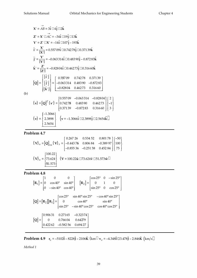
AB→
= −( ) + −( ) + −( ) = + +4 1 6 2 5 3 3 4 2ˆ ˆ ˆ ˆ ˆ ˆi j k i j k
AC→
= −( ) + −( ) + − −( ) = + −3 1 9 2 2 3 2 7 5ˆ ˆ ˆ ˆ ˆ ˆi j k i j k
Solutions Manual Orbital Mechanics for Engineering Students Chapter 4
39
′ = = + +→
X i j kAB 3 4 2ˆ ˆ ˆ
′ = ′ × = − + +→
Z X i j kAC 34 19 13ˆ ˆ ˆ
′ = ′ × ′ = − + −Y Z X i j k14 107 193ˆ ˆ ˆ
ˆ . ˆ . ˆ . ˆ′ =′
′= + +i
XX
i j k0 557 09 0 74278 0 37139
ˆ . ˆ . ˆ . ˆ′ =′
′= − + −j
YY
i j k0 063 314 0 483 90 0 872 83
ˆ . ˆ . ˆ . ˆ′ =′
′= − + +k
ZZ
i j k0 82804 0 46273 0 316 60
Q
i
j
k
[ ] =
′
′
′
=
ˆ
ˆ
ˆ
.0 5557 09 0 74278 0 371390 063 314 0 483 90 0 872 83
. .. . .− −
−−
0 82804 0 46273 0 316 60. . .
(b)
v Q v = [ ] ′ =
− −T
0 557 09 0 063 314 0 828040 7427. . .. 88 0 483 90 0 46273
0 37139 0 872 83 0 316 60. .
. . .−
−
=
−
21
3
1 30662 38982 5654
v
...
= − + + . ˆ . ˆ .v i j1 3066 2 3898 2 5654 ˆk( )
Problem 4.7
V Q V = [ ] = −u xu x
0 267 26 0 534 52 0 801 780 443 7. . .. 66 0 806 84 0 389 97
0 855 36 0 251 58 0 452 84. .
. . .−
− −
−
=
5010075
100 2273 624V u
..
551 573100 22 73 624 51
. . ˆ . ˆ
= + +V u v .. ˆ573w( )
Problem 4.8
R R1 2
1 0 00 40 400 40 40
25 0 250 1 025 0 25
[ ] = ° °
− ° °
[ ] =
° − °
° °
cos sinsin cos
cos sin
sin cos
Q R R[ ] = [ ][ ] =
° ° ° − ° °
° °
° − ° ° ° °
2 1
25 40 25 40 250 40 4025 40 25 40 25
cos sin sin cos sincos sin
sin sin cos cos cos
Q[ ] =
−
−
0 906 31 0 27165 0 323740 0 766 04 0 64279
0 422 62 0 582 56 0 694 27
. . .. .
. . .
Problem 4.9 r I J K v Io o= − − − ( ) = −5102 8228 2106 4 348ˆ ˆ ˆ . ˆ km ++ − ( )3 478 2 846. ˆ . ˆJ K km s
Method 1
Solutions Manual Orbital Mechanics for Engineering Students Chapter 4
40
Use Algorithm 3.4 (MATLAB M-function rv_from_r0v0 in Appendix D.7):
1 9907 6 6 2531
1
a r v
bo o( ) = =
( ) . . km km s
.
.
v
c
ro = −
( ) = × −
0 044 678
1 103 77 10 6
km s
α kkm
km
-1
1/22 195
3 0 365 39
( ) =
( ) = −
.
χ
f .
. ˆg =
( ) = −( ) − −
1394 4
4 0 36 539 5102 82
s-1
r I 228 2106 1394 4 4 348 3 478 2 846ˆ ˆ . . ˆ . ˆ .J K I J−( ) + − + − ˆ
. ˆ . ˆ . ˆK
I J K
( )= − + − (4198 4 7856 1 3199 2 km))
( ) = − × = −
(
−5 6 0467 10 0 429 31
6
4 . .f g s-1
)) = − ×( ) − − −( )− . ˆ ˆ ˆv I J K6 0467 10 5102 8228 21064 ++ −( ) − + −( )0 429 31 4 348 3 478 2 846. . ˆ . ˆ . ˆ
I J K
== + + ( )4 9517 3 4821 2 4946. ˆ . ˆ . ˆI J K km s
Method 2
Compute the orbital elements using Algorithm 4.1 (MATLAB M-function coe_from_sv in AppendixD.8):
1 9907 6
2 6 2531
3
( ) = =
( ) = =
( )
.
.
r
v
v
r
v
km
km s
rr r=
⋅= − <( )
( ) = × =
r v
h r v
0 044 678 0
4 3073
.
km s
88 5367 8 53 520
5 6
ˆ . ˆ ˆ
I J K
h
− − ( )( ) = =
km s
1 952
2
h km s
1 9
2
653 520
61 1( ) =
=−− − cos cosi
hhZ
552
= °
( ) = × = +
149 76
7 5367 8 30738
.
ˆ . ˆN K h I ˆ
c
J
N
km s
km s
2
2
( ) >( )( ) = =
( ) =
N
N
Y 0
8 31 203
9 Ω oos cos.
.− −
=
=1 1 5367 8
31 20380 09
NN
X 44°
101
398 6005 7415 398 600 9907 6 51022( ) = −( ) − . . ˆe II J K− −( )
−
8228 2106
9907 6
ˆ ˆ
.(( ) −( ) − + −( )=
0 044 678 4 348 3 478 2 846. . ˆ . ˆ . ˆI J K
00 009 638 51 0 027193 0 002 808 3 0. ˆ . ˆ . ˆ I J K+ + >eZ(( )
( ) .
( ) cos .
( ) cos . .
11 0 028 987
12 11 09
13 360 360 166 14 193 86
1
1
e
Ne
er
= =
⋅
= °
= ° −⋅
= ° − ° = °
−
−
e
N e
e r
ω
θ
==
Th
e=
−
=
2
19414 92 2
3π
µ. s
Determine the time since perigee passage at true anomaly θo = °193 86. :
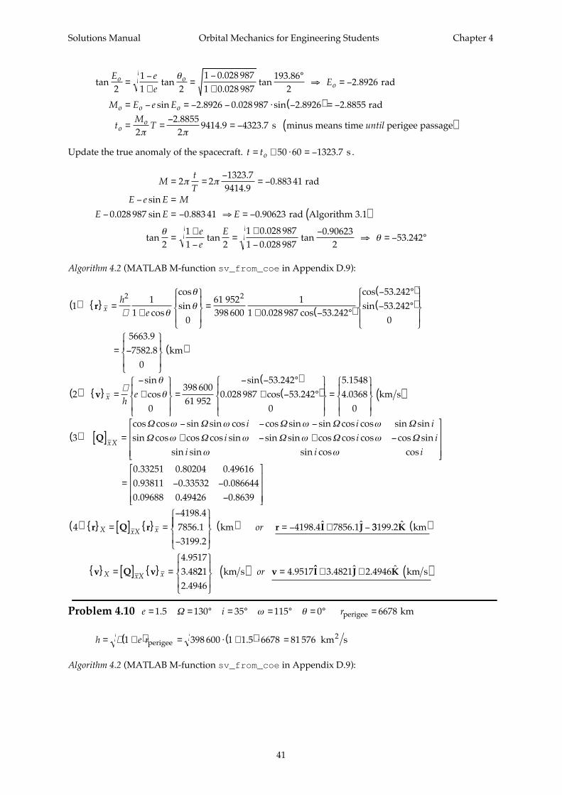
Solutions Manual Orbital Mechanics for Engineering Students Chapter 4
41
tan tan..
tan.
.
sin . . sin . ..
. .
E ee
E
M E e E
tM
T until
o oo
o o o
oo
211 2
1 0 028 9871 0 028 987
193 862
2 8926
2 8926 0 028 987 2 8926 2 8855
22 88552
9414 9 4323 7
=−+
=−
+°
⇒ = −
= − = − − ⋅ −( ) = −
= =−
= − ( )
θ
π π
rad
rad
s minus means time perigee passage
Update the true anomaly of the spacecraft. t to= + ⋅ = −50 60 1323 7. s .
MtT
E e E M
E E E
ee
E
= =−
= −
− =
− = − ⇒ = − ( )
=+−
=+
−−
⇒ = − °
2 21323 7
9414 90 883 41
0 028 987 0 883 41 0 90623
211 2
1 0 028 9871 0 028 987
0 906232
53 242
π π
θθ
..
.
sin
. sin . .
tan tan..
tan.
.
rad
rad Algorithm 3.1
Algorithm 4.2 (MATLAB M-function sv_from_coe in Appendix D.9):
11
10
6398 600
11 0 028 987 53 242
53 24253 2420
5663 97582 8
0
2 2( ) =
+
=+ − °( )
− °( )
− °( )
= −
( )
cos
cossin
. cos .
cos .sin .
..
r xh
eµ θ
θ
θ1 952
km
20
398 6006
53 2420 028 987 53 242
0
5 15484 0368
0
( ) =
−
+
=
− − °( )
+ − °( )
=
( ) sincos
sin .. cos .
.
.v x he
µθ
θ1 952
km s
3
0 33251 0 80204 0 496160 93811 0 33532 0 0866440 09688 0
( ) [ ] =
− − −
+ − + −
= − −
cos cos sin sin cos cos sin sin cos cos sin sinsin cos cos cos sin sin sin cos cos cos cos sin
sin sin sin cos cos
. . .. . ..
Q xX
i i i
i i i
i i i
Ω Ω Ω Ω Ω
Ω Ω Ω Ω Ω
ω ω ω ω
ω ω ω ω
ω ω
.. .49426 0 8639−
44198 4
7856 13199 2
( ) = [ ] =
−
−
.
..
r Q rX xX x
( ) = − + − km . ˆ . ˆor r I J4198 4 7856 1 33199 2
4 95173 48
. ˆ
..
K
v Q v
km( )
= [ ] =X xX x 2212 4946
4 9517.
.
( ) = km s or v ˆ . ˆ . ˆI J K+ + ( )3 4821 2 4946 km s
Problem 4.10 e i r= = ° = ° = ° = ° =1 5 130 35 115 0 6678. Ω ω θ perigee km
h e r= +( ) = ⋅ +( ) ⋅ =µ 1 398 600 1 1 5 6678 81 576perigee
2 km s.
Algorithm 4.2 (MATLAB M-function sv_from_coe in Appendix D.9):
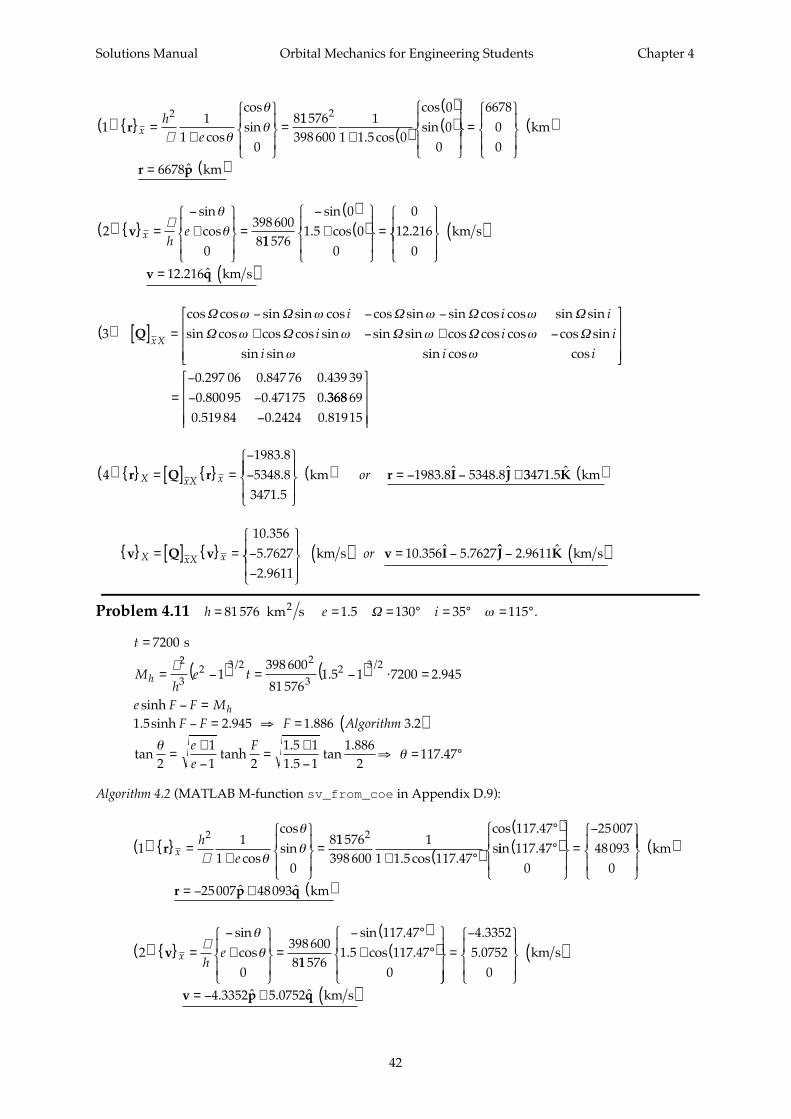
Solutions Manual Orbital Mechanics for Engineering Students Chapter 4
42
11
10
82( ) =
+
= cos
cossinr x
heµ θ
θ
θ11576
398 6001
1 1 5 0
00
0
2
+ ( )
( )( )
. cos
cossin
=
( )
=
667800
6678
km
ˆr p km( )
20
398 6008
( ) =
−
+
= sincosv x h
eµ
θ
θ11576
01 5 0
0
012 216
0
− ( )+ ( )
=
sin. cos .
( )
= ( )
km s
km s . ˆv q12 216
3
0 297 06 0 847 76 0 439 390 800 95 0 47175 0
( ) [ ] =
− − −
+ − + −
=
−
− −
cos cos sin sin cos cos sin sin cos cos sin sinsin cos cos cos sin sin sin cos cos cos cos sin
sin sin sin cos cos
. . .. . .
Q xX
i i i
i i i
i i i
Ω Ω Ω Ω Ω
Ω Ω Ω Ω Ω
ω ω ω ω
ω ω ω ω
ω ω
368368 690 519 84 0 2424 0 81915. . .−
41983 85348 8
3471 5
( ) = [ ] =
−
−
..
.r Q rX xX x
( ) = − − + km . ˆ . ˆor r I J1983 8 5348 8 33471 5. K km( )
...
v Q v = [ ] = −
−
X xX x
10 3565 76272 9611
( ) = − km s . ˆ .or v I10 356 5 7627ˆ . ˆJ K− ( )2 9611 km s
Problem 4.11 h e i= = = ° = ° = °81 576 1 5 130 35 115 km s2 . Ω ω .
t = 7200 s
M
he th = −( ) = −( ) ⋅ =
µ2
32 3 2 2
32 3 2
1398 600
81 5761 5 1 7200 2 945
/ /. .
e F F Mhsinh − =
1 5 2 945 1 886. sinh . . F F F− = ⇒ = ( )Algorithm 3.2
tan tanh
.
.tan
. .
θθ
211 2
1 5 11 5 1
1 8862
117 47=+−
=+−
⇒ = °ee
F
Algorithm 4.2 (MATLAB M-function sv_from_coe in Appendix D.9):
11
10
82( ) =
+
= cos
cossinr x
heµ θ
θ
θ11576
398 6001
1 1 5 117 47
117 472
+ °( )
°( )
. cos .
cos .siin .117 47
0
2500748093
0°( )
=
−
( )
= − + ( )
km
km ˆ ˆr p q25007 48093
20
398 6008
( ) =
−
+
= sincosv x h
eµ
θ
θ11576
117 471 5 117 47
0
− °( )+ °( )
sin .. cos .
=
−
( )4 3352
5 07520
..
km s
. ˆ . ˆv p q= − + ( )4 3352 5 0752 km s
Solutions Manual Orbital Mechanics for Engineering Students Chapter 4
43
30 297 06 0 847 76 0 439 390 800 95 0 47175 0 368 69
0 519 84 0 2424 0 81915
( ) [ ] =
−
− −
−
( ) . . .. . .
. . .Q xX Problem 4.10
448 200
265824 658
( ) = [ ] = −
−
r Q rX xX x
( ) = − − km ˆ ˆ ˆor r I J K48 200 2658 24 658 kkm( )
= [ ] =
−
..v Q vX xX x
5 59031 07813..
. ˆ
48385 5903
( ) = + km s or v I 11 0781 3 4838. ˆ . ˆJ K− ( ) km s
Problem 4.12 r I J K vo = − − ( ) =6472 7 7470 8 2469 8 3. ˆ . ˆ . ˆ . km o 99914 2 7916 3 2948ˆ . ˆ . ˆI J K+ − ( ) km s2
Method 1
Use Algorithm 3.4 (MATLAB M-function rv_from_r0v0 in Appendix D.7):
1 10189 5 805
1
a r v
bo o( ) = =
( ) .
km km s
.
.
v
c
ro =
( ) = × −
1 2874
1 109 54 10
2
6
km s
km-1α
(( ) =
( ) = −
.
.
χ 171 31
3 0 093 379
km1/2
f .
. . ˆg =
( ) = −( ) −
1870 6
4 0 093 379 6472 7 7
s-1
r I 4470 8 2469 8 1870 6 3 9914 2 7916. ˆ . ˆ . . ˆ . ˆJ K I J−( ) + + −−( )= + −
3 2948
6861 9 5919 6 5932 7
. ˆ
. ˆ . ˆ .
K
I J ˆ
. .
K km
s-1
( )
( ) = − × = −−5 5 3316 10 0 04f g 228 475
6 5 3316 10 6472 7 7470 84( ) = − ×( ) −− . . ˆ . ˆv I JJ K I J−( ) + −( ) + −2469 8 0 028 475 3 9914 2 7916. ˆ . . ˆ . ˆ 33 2948
3 5647 3 9037 1 4106
. ˆ
. ˆ . ˆ . ˆK
I J
( )= − + + KK km s( )
Method 2
From Problem 4.3 h e i= = = ° = ° = ° = °5 0 2465 35 110 74 996 1308 461 km s2 , . , , , . , Ω ω θ .
Th
e
E ee
E
M E e E
o oo
o o o
=−
=
−
=
=−+
=−+
°⇒ =
= − = − ⋅ ( ) =
2
1
2
398 600
5
1 0 24658680 3
211 2
1 0 24651 0 2465
1302
2 0612
2 0612 0 2465 2 0612 1 8437
2 2
3
2 2
3π
µ
π
θ
8 461 s
rad
..
tan tan..
tan .
sin . . sin . . rad rad
s minus means time perigee passagetM
T untiloo= = = ( )
21 8437
28680 3 2547 1
π π.
. .
Update the true anomaly: t to= + ⋅ =50 60 5547 1. s
Solutions Manual Orbital Mechanics for Engineering Students Chapter 4
44
MtT
E e E M
E E E
ee
E
= = =
− =
− = ⇒ = ( )
=+−
=+−
⇒ = − °
2 25547 18680 3
4 0153
0 2465 4 0153
211 2
1 0 24651 0 2465 2
147 73
π π
θθ
.
..
sin
. sin .
tan tan..
tan .
rad
3.8541 rad Algorithm 3.1
3.8541
Algorithm 4.2 (MATLAB M-function sv_from_coe in Appendix D.9):
11
10
58 461398 600
11 0 2465 147 73
147 73147 730
9158 15783 8
0
2 2( ) =
+
=+ − °( )
− °( )
− °( )
=
−
−
( )
cos
cossin
. cos .
cos .sin .
..
r xh
eµ θ
θ
θ
km
20
398 6008 461
147 730 2465 147 73
0
3 64084 0841
0
( ) =
−
+
=
− − °( )
+ − °( )
= −
( ) sincos
sin .. cos .
..v x h
eµ
θ
θ km s
3
0 8321 0 13078 0 538 990 026 991 0 9802 0 19617
( ) [ ] =
− − −
+ − + −
=
−
− −
cos cos sin sin cos cos sin sin cos cos sin sinsin cos cos cos sin sin sin cos cos cos cos sin
sin sin sin cos cos
. . .
. . .
Q xX
i i i
i i i
i i i
Ω Ω Ω Ω Ω
Ω Ω Ω Ω Ω
ω ω ω ω
ω ω ω ω
ω ω
00 553 97 0 148 69 0 81915. . .
46864
5916 55933 3
( ) = [ ] =
−
..
r Q rX xX x
( ) = + − km ˆ . ˆ .or r I J6864 5916 5 5933 3 ˆ
..
.
K
v Q v
km( )
= [ ] =
−
X xX x
3 56363 905
1 409963 5636 3
( ) = − + km s . ˆ .or v I 9905 1 4096ˆ . ˆJ K+ ( ) km s
Problem 4.13 e i r= = ° = ° = ° = ° =1 2 75 50 80 0 6578. Ω ω θ perigee km
h e r= +( ) = ⋅ +( ) ⋅ =µ 1 398 600 1 1 2 6578 79 950perigee
2 km s.
Algorithm 4.2 (MATLAB M-function sv_from_coe in Appendix D.9):
11
10
72( ) =
+
= cos
cossinr x
heµ θ
θ
θ99 950
398 6001
1 1 2 0
00
0
2
+ ( )
( )( )
. cos
cossin
=
( )
=
657800
6578
km
ˆr p km( )
20
398 6007
( ) =
−
+
= sincosv x h
eµ
θ
θ99 950
01 2 0
0
011 546
0
− ( )+ ( )
=
sin. cos .
( )
= ( )
km s
km s . ˆv q11 546
Solutions Manual Orbital Mechanics for Engineering Students Chapter 4
45
3
0 56 561 0 3627 0 739 940 331 57 0 92236 0 198
( ) [ ] =
− − −
+ − + −
=
− −
− −
cos cos sin sin cos cos sin sin cos cos sin sinsin cos cos cos sin sin sin cos cos cos cos sin
sin sin sin cos cos
. . .
. . .
Q xX
i i i
i i i
i i i
Ω Ω Ω Ω Ω
Ω Ω Ω Ω Ω
ω ω ω ω
ω ω ω ω
ω ω
27270 754 41 0 133 02 0 64279. . .
43726 5
2181 14962 5
( ) = [ ] =
−
...
r Q rX xX x
( ) = − + + km . ˆ . ˆor r I J3726 5 2181 1 49962 5
4 187810 6
. ˆ
.
.
K
v Q v
km( )
= [ ] =
−
−X xX x 551 5359
4 1878.
.
( ) = − km s or v ˆ . ˆ . ˆI J K+ + ( )10 65 1 5359 km s
Problem 4.14 h e i= = = ° = ° = °75950 1 2 130 50 80 km s2 . Ω ω
t
Mh
e t
e F F M
F F F
ee
F
h
h
=
= −( ) = −( ) ⋅ =
− =
− = ⇒ = ( )
=+−
=+−
⇒ =
7200
1398 600
759501 2 1 7200 0 762 09
1 2 0 762 09 1 3174
211 2
1 2 11 2 1
0 762 092
124
2
32 3 2 2
32 3 2
s
3.2
µ
θθ
/ /. .
sinh
. sinh . .
tan tanh..
tan.
.
Algorithm
8686°
Algorithm 4.2 (MATLAB M-function sv_from_coe in Appendix D.9):
11
10
72( ) =
+
= cos
cossinr x
heµ θ
θ
θ55950
398 6001
1 1 2 124 86
124 862
+ °( )
°( )
. cos .
cos .siin .124 86
0
26 33637 806
0°( )
=
−
( )
= − + ( )
km
km ˆ ˆr p q26 336 37 806
20
398 6008
( ) =
−
+
= sincosv x h
eµ
θ
θ11576
124 861 5 124 86
0
− °( )+ °( )
sin .. cos .
=
−
( )4 30643 298
0
.
.
km s
vv p q= − + ( )4 3064 3 298. ˆ . ˆ km s
30 56 561 0 3627 0 739 94
0 331 57 0 92236 0 198 270 754 41 0 133 02 0 64279
( ) [ ] =
− −
− −
( ) . . .
. . .
. . .Q xX Problem 4.13
41207 243 60314 839
( ) = [ ] = −
−
.
r Q rX xX x
( ) = − − km . ˆ ˆor r I J1207 2 43 603 14 8399
1 24344 4
ˆ
..
K
v Q v
km( )
= [ ] = −X xX x 66982 8100
1 24−
( ) =
. . km s or v 334 4 4698 2 8100ˆ . ˆ . ˆI J K− − ( ) km s
Solutions Manual Orbital Mechanics for Engineering Students Chapter 4
46
60°
X
Y
ZB
perigeeapogee
Problem 4.15 h e= = = °75000 0 7 25 km s2 . θ
v =
−
+
=
− °( )
+ °( )
=
−
( )x he
µθ
θ
sincos
sin. cos
..
0
398 60075000
250 7 25
0
2 24618 537
0 km s
v Q v = [ ] =
−
−
= −
−
( )X xX x . .
....
0 83204 2 24618 537
0
2 10288 07332 8853
0.02741 0.55403-0.13114 -0.98019 -0.148450.53899 -0.19617 0.81915
km s
or
v I J K= − − ( )2 1028 8 0733 2 8853. ˆ . ˆ . ˆ km s
Problem 4.16
Ω = ° = = °60 0 90 ω i
v =
−
−
( )x
3 2080 8288
0
.. km s
cos cos sin sin cos cos sin sin cos cos sin sinsin cos cos cos sin sin sin cos cos cos cos sin
sin sin sin cos cos
. .. .
Q[ ] =
− − −
+ − + −
= −
xX
i i i
i i i
i i i
Ω Ω Ω Ω Ω
Ω Ω Ω Ω Ω
ω ω ω ω
ω ω ω ω
ω ω
0 5 0 0 866030 86603 0 0 5
0 1 0
v Q v = =
−
−
−
X xX x ...
1 6042 77820 8288
( )
= − − −
km s
or
v I J K1 604 2 7782 0 8288. ˆ . ˆ . ˆ kkm s( )
Problem 4.17 a e i= = = ° = = ° = °7016 0 05 45 0 20 10 km . Ω ω θ
r =−( )
+
=−( )
+ °
°
°
=
( )xa e
e1
10
7016 1 051 0 05 10
1010
0
6568 71158 2
0
2 2
cos
cossin
. cos
cossin
.
.θ
θ
θ km
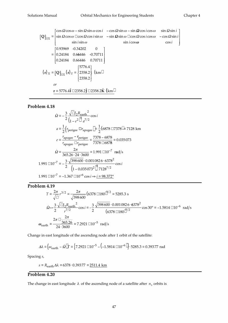
Solutions Manual Orbital Mechanics for Engineering Students Chapter 4
47
cos cos sin sin cos cos sin sin
Q =
− − −
xX
iΩ Ω Ωω ω ω ΩΩ Ω
Ω Ω
cos cos sin sinsin cos cos cos sin sin
i i
i
ω
ω ω+ − ΩΩ Ω Ωsin cos cos cos cos sinsin sin sin cos
ω ω
ω
+ −i i
i i ωω cos i
=
0.93969 -0.342020.24184 0.6
066446 -0.70711
0.24184 0.66446 0.70711
= =
r Q rX xX x
5776 42358 22358 2
.
.
.
( )
= + +
km
km
or
r I J K5776 4 2358 2 2358 2. ˆ . ˆ . ˆ (( )
Problem 4.18
Ω = −−( )
=
32
112
22
2 2 7 2
µ J R
e ai
a r
earth
perigee
/cos
++( ) = +( ) =
=−
r
er
apogee
apogee
km12
6878 7378 7128
rr
r rperigee
apogee perigee+=
−+
7378 68787378 68788
0 035073
2365 26 24 3600
1 991 10 7
=
=⋅ ⋅
= × −
.
..Ω
π raad s
1 991 1032
398 600 0 001082 6 6378
1 0
72
..
× = −⋅ ⋅
−
−
..cos
. .
/035073 7128
1 991 10 1 367 10
2 2 7 2
7
( )× = − ×−
i
−− ⇒ = °6 98 372cos .i i
Problem 4.19
T r= = +( ) =2 2
398 6006378 180 5285 33 2 3 2π
µ
π/ / . s
=Ω --32
-32
earthµ J R
ri2
2
7 2
398 600 0 001082 6/
cos.
=⋅ ⋅66378
6378 18030 1 5814 10
2
7 26
+( )° = − × −
/cos . rad s
ωωπ
π
earth rad s=+
⋅= × −
22
365 2624 3600
7 2921 10 5. .
Change in east longitude of the ascending node after 1 orbit of the satellite:
∆ Ωλ ω= −( ) = × − − ×( ) − −
earth T 7 2921 10 1 5814 105 6. . ⋅ =5285 3 0 39377. . rad
Spacing s,
s R= = ⋅ =earth km∆λ 6378 0 39377 2511 4. .
Problem 4.20
The change in east longitude λ of the ascending node of a satellite after ns orbits is
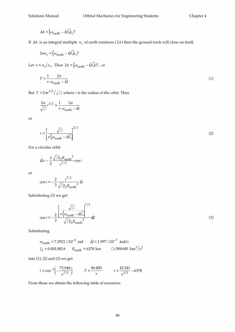
Solutions Manual Orbital Mechanics for Engineering Students Chapter 4
48
∆ Ωλ ω= −( )earth n Ts
If ∆λ is an integral multiple ne of earth rotations ( 2π ) then the ground track will close on itself,
2π ωn n Te s= −( )earth Ω
Let ν = n ns e . Then 2π ω ν= −( )earth Ω T , or
T =
−
1 2ν
π
ωearth Ω(1)
But T r= 2 3 2π µ/ , where r is the radius of the orbit. Thus
2 1 23 2π
µ νπ
ωr / =
−earth Ω
or
r =−( )
µ
ν ωearth Ω
2 3/
(2)
For a circular orbit
Ω=
32
earth−µ J R
ri2
2
7 2/cos
or
cos
/i
r
J R= −
23
7 2
22µ earth
Ω
Substituting (2) we get
cos
/
iJ R
= −−( )
2
3
7 3
22
µ
ν ω
µ
earth
earth
ΩΩΩ (3)
Substituting
ωearth rad = × = ×− −7 2921 10 1 997 105 7. .Ω rrad s
km earthJ R2 0 001082 6 6378= =. =398 600 km s3 2µ
into (1), (2) and (3) we get
i T z= −
= = −−cos
. / /
17 3 2 3
73 948 86 400 42 2416378
ν ν ν
From these we obtain the following table of scenarios:
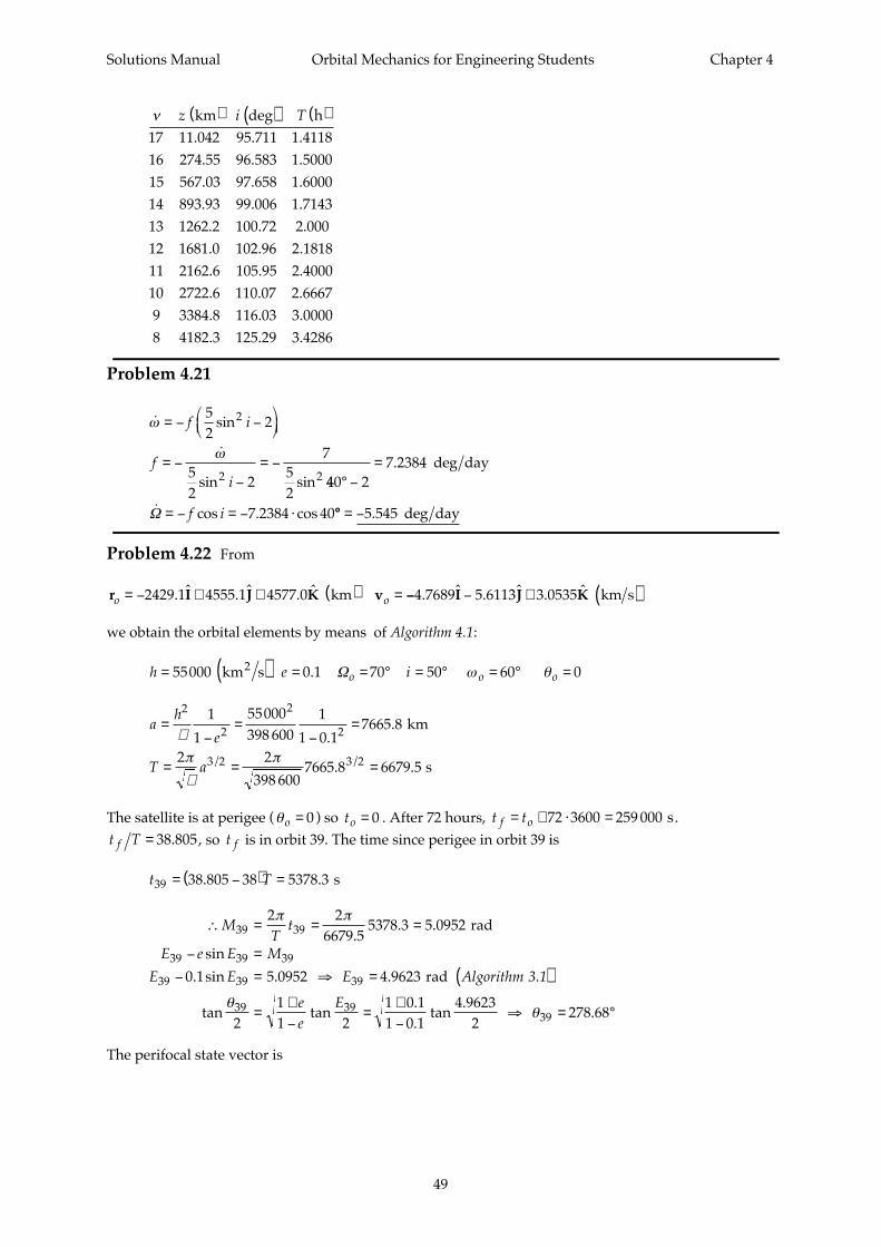
Solutions Manual Orbital Mechanics for Engineering Students Chapter 4
49
ν z i T km deg h17 11.042 95.711 1.411816 274.55 96.583 1.500015 567.03 97.658 1.600014 893.93 1.714313 1262.2 2.00012 1681.0 2.181811 2162.6 2.400010 2722.6 2.66679 3384.8 3.00008 4182.3 3.4286
( ) ( ) ( )
99 006100 72102 96105 95110 07116 03125 29
.......
Problem 4.21
ω
ω
= − −
= −−
= −
f i
fi
52
2
52
2
752
2
2 2
sin
sin sin 440 27 2384
7 2384 40
° −=
= − = − ⋅
.
cos . cos
deg day
Ω f i °° = −5 545. deg day
Problem 4.22 From
r I J K vo o= − + + ( ) =2429 1 4555 1 4577 0. ˆ . ˆ . ˆ km −− − + ( )4 7689 5 6113 3 0535. ˆ . ˆ . ˆI J K km s
we obtain the orbital elements by means of Algorithm 4.1:
h e io o o= ( ) = = ° = ° = ° =55000 0 1 70 50 60 0 km s2 . Ω ω θ
ah
e
T a
=−
=−
=
= = =
2
2
2
2
3 2 3 2
1
1
55000398 600
1
1 0 17665 8
2 2
398 6007665 8 6679 5
µ
π
µ
π.
.
. ./ /
km
s
The satellite is at perigee ( θo = 0 ) so to = 0 . After 72 hours, t tf o= + ⋅ =72 3600 259 000 s.
t Tf = 38 805. , so
t f is in orbit 39. The time since perigee in orbit 39 is
t T39 38 805 38 5378 3= −( ) =. . s
∴ = = =
− =
− = ⇒ = ( )
=+−
=+−
⇒ = °
MT
t
E e E M
E E E
ee
E
39 39
39 39 39
39 39 39
39 3939
2 26679 5
5378 3 5 0952
0 1 5 0952 4 9623
211 2
1 0 11 0 1
4 96232
278 68
π π
θθ
.. .
sin
. sin . .
tan tan..
tan.
.
rad
rad Algorithm 3.1
The perifocal state vector is
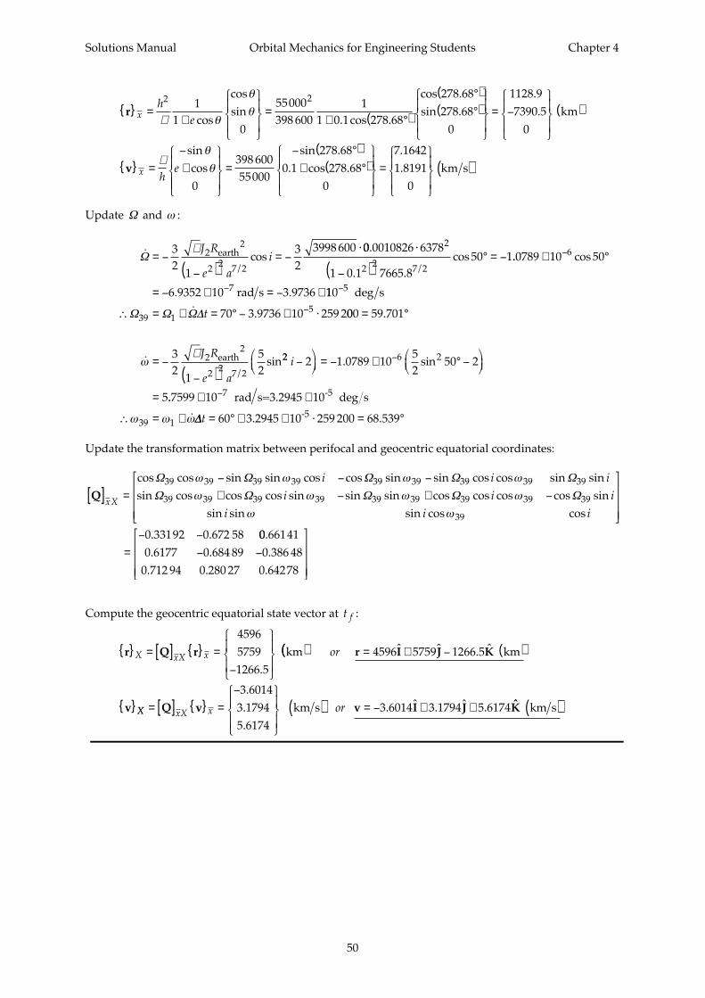
Solutions Manual Orbital Mechanics for Engineering Students Chapter 4
50
r
v
=+
=+ °( )
°( )
°( )
= −
( )
=
−
+
x
x
he
he
2 211
0
55000398 600
11 0 1 278 68
278 68278 68
0
1128 97390 5
0
0
µ θ
θ
θ
µθ
θ
cos
cossin
. cos .
cos .sin .
..
sincos
km
=
− °( )
+ °( )
=
( )398 60055000
278 680 1 278 68
0
7 16421 8191
0
sin .. cos .
.
. km s
Update Ω and ω :
Ω = −−( )
= −⋅3
21
32
3998 60022
2 2 7 2
µ J R
e aiearth
/cos
00 0010826 6378
1 0 1 7665 850 1
2
2 2 7 2
.
. .cos
/
⋅
−( )° = − .. cos
. .
0789 10 50
6 9352 10 3 9736
6
7
× °
= − × = − ×
−
− rad s 110
70 3 9736 10 259 2
5
39 15
−
−∴ = + = ° − × ⋅
deg s
Ω Ω Ω∆t . 000 59 701
32
1
52
22
2 2 7 2
= °
= −−( )
.
sin/
ωµ J R
e a
earth 22 6 22 1 0789 1052
50 2
5
i −
= − × ° −
=
−. sin
..7599 10 7
39 1
× ×
∴ = +
− rad s=3.2945 10 deg s-5
ω ω ω∆∆t = ° + × ⋅ = °60 259 200 68 5393.2945 10-5 .
Update the transformation matrix between perifocal and geocentric equatorial coordinates:
Q[ ] =
− − −
+ − + −
=
− −
xX
i i i
i i i
i i i
cos cos sin sin cos cos sin sin cos cos sin sinsin cos cos cos sin sin sin cos cos cos cos sin
sin sin sin cos cos
. .
Ω Ω Ω Ω Ω
Ω Ω Ω Ω Ω39 39 39 39 39 39 39 39 39
39 39 39 39 39 39 39 39 39
39
0 33192 0 672 58
ω ω ω ω
ω ω ω ω
ω ω
00 661410 6177 0 684 89 0 386 48
0 712 94 0 280 27 0 64278
.. . .
. . .− −
Compute the geocentric equatorial state vector at t f :
r Q r = [ ] =
−
X xX x
459657591266 5.
km(( ) = + − ( )
ˆ ˆ . ˆor r I J K
v
4596 5759 1266 5 km
XX xX x= [ ] =
−
Q v
3 60143 17945 6174
...
km s( ) = − + + . ˆ . ˆ .or v I J3 6014 3 1794 5 6174 ˆK km s( )
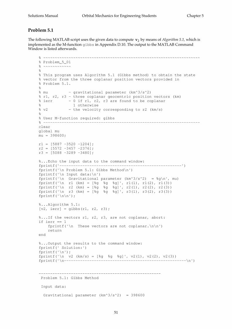
Solutions Manual Orbital Mechanics for Engineering Students Chapter 5
51
Problem 5.1
The following MATLAB script uses the given data to compute v2 by means of Algorithm 5.1, which isimplemented as the M-function gibbs in Appendix D.10. The output to the MATLAB CommandWindow is listed afterwards.
% ~~~~~~~~~~~~~~~~~~~~~~~~~~~~~~~~~~~~~~~~~~~~~~~~~~~~~~~~~~~~~~~~~~~~% Problem_5_01% ~~~~~~~~~~~~%% This program uses Algorithm 5.1 (Gibbs method) to obtain the state% vector from the three coplanar position vectors provided in% Problem 5.1.%% mu - gravitational parameter (km^3/s^2)% r1, r2, r3 - three coplanar geocentric position vectors (km)% ierr - 0 if r1, r2, r3 are found to be coplanar% 1 otherwise% v2 - the velocity corresponding to r2 (km/s)%% User M-function required: gibbs% --------------------------------------------------------------------clearglobal mumu = 398600;
r1 = [5887 -3520 -1204];r2 = [5572 -3457 -2376];r3 = [5088 -3289 -3480];
%...Echo the input data to the command window:fprintf('-----------------------------------------------------')fprintf('\n Problem 5.1: Gibbs Method\n')fprintf('\n Input data:\n')fprintf('\n Gravitational parameter (km^3/s^2) = %g\n', mu)fprintf('\n r1 (km) = [%g %g %g]', r1(1), r1(2), r1(3))fprintf('\n r2 (km) = [%g %g %g]', r2(1), r2(2), r2(3))fprintf('\n r3 (km) = [%g %g %g]', r3(1), r3(2), r3(3))fprintf('\n\n');
%...Algorithm 5.1:[v2, ierr] = gibbs(r1, r2, r3);
%...If the vectors r1, r2, r3, are not coplanar, abort:if ierr == 1 fprintf('\n These vectors are not coplanar.\n\n') returnend
%...Output the results to the command window:fprintf(' Solution:')fprintf('\n');fprintf('\n v2 (km/s) = [%g %g %g]', v2(1), v2(2), v2(3))fprintf('\n-----------------------------------------------------\n')
----------------------------------------------------- Problem 5.1: Gibbs Method
Input data:
Gravitational parameter (km^3/s^2) = 398600
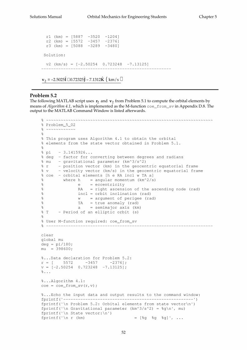
Solutions Manual Orbital Mechanics for Engineering Students Chapter 5
52
r1 (km) = [5887 -3520 -1204] r2 (km) = [5572 -3457 -2376] r3 (km) = [5088 -3289 -3480]
Solution:
v2 (km/s) = [-2.50254 0.723248 -7.13125]-----------------------------------------------------
v I J K2 2 5025 0 72325 7 1312= − + − ( ). ˆ . ˆ . ˆ km/s
Problem 5.2The following MATLAB script uses r2 and v2 from Problem 5.1 to compute the orbital elements bymeans of Algorithm 4.1, which is implemented as the M-function coe_from_sv in Appendix D.8. Theoutput to the MATLAB Command Window is listed afterwards.
% ~~~~~~~~~~~~~~~~~~~~~~~~~~~~~~~~~~~~~~~~~~~~~~~~~~~~~~~~~~~~~~~~~~~~% Problem_5_02% ~~~~~~~~~~~~%% This program uses Algorithm 4.1 to obtain the orbital% elements from the state vector obtained in Problem 5.1.%% pi - 3.1415926...% deg - factor for converting between degrees and radians% mu - gravitational parameter (km^3/s^2)% r - position vector (km) in the geocentric equatorial frame% v - velocity vector (km/s) in the geocentric equatorial frame% coe - orbital elements [h e RA incl w TA a]% where h = angular momentum (km^2/s)% e = eccentricity% RA = right ascension of the ascending node (rad)% incl = orbit inclination (rad)% w = argument of perigee (rad)% TA = true anomaly (rad)% a = semimajor axis (km)% T - Period of an elliptic orbit (s)%% User M-function required: coe_from_sv% --------------------------------------------------------------------
clearglobal mudeg = pi/180;mu = 398600;
%...Data declaration for Problem 5.2:r = [ 5572 -3457 -2376];v = [-2.50254 0.723248 -7.13125];%...
%...Algorithm 4.1:coe = coe_from_sv(r,v);
%...Echo the input data and output results to the command window:fprintf('-----------------------------------------------------')fprintf('\n Problem 5.2: Orbital elements from state vector\n')fprintf('\n Gravitational parameter (km^3/s^2) = %g\n', mu)fprintf('\n State vector:\n')fprintf('\n r (km) = [%g %g %g]', ...
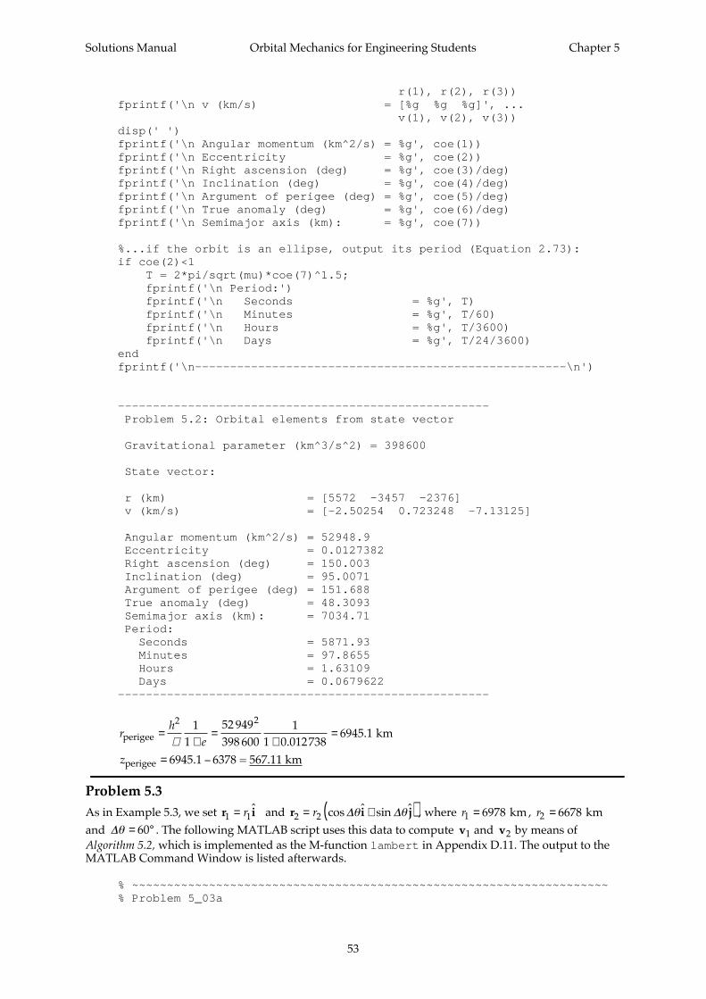
Solutions Manual Orbital Mechanics for Engineering Students Chapter 5
53
r(1), r(2), r(3))fprintf('\n v (km/s) = [%g %g %g]', ... v(1), v(2), v(3))disp(' ')fprintf('\n Angular momentum (km^2/s) = %g', coe(1))fprintf('\n Eccentricity = %g', coe(2))fprintf('\n Right ascension (deg) = %g', coe(3)/deg)fprintf('\n Inclination (deg) = %g', coe(4)/deg)fprintf('\n Argument of perigee (deg) = %g', coe(5)/deg)fprintf('\n True anomaly (deg) = %g', coe(6)/deg)fprintf('\n Semimajor axis (km): = %g', coe(7))
%...if the orbit is an ellipse, output its period (Equation 2.73):if coe(2)<1 T = 2*pi/sqrt(mu)*coe(7)^1.5; fprintf('\n Period:') fprintf('\n Seconds = %g', T) fprintf('\n Minutes = %g', T/60) fprintf('\n Hours = %g', T/3600) fprintf('\n Days = %g', T/24/3600)endfprintf('\n-----------------------------------------------------\n')
----------------------------------------------------- Problem 5.2: Orbital elements from state vector
Gravitational parameter (km^3/s^2) = 398600
State vector:
r (km) = [5572 -3457 -2376] v (km/s) = [-2.50254 0.723248 -7.13125]
Angular momentum (km^2/s) = 52948.9 Eccentricity = 0.0127382 Right ascension (deg) = 150.003 Inclination (deg) = 95.0071 Argument of perigee (deg) = 151.688 True anomaly (deg) = 48.3093 Semimajor axis (km): = 7034.71 Period: Seconds = 5871.93 Minutes = 97.8655 Hours = 1.63109 Days = 0.0679622-----------------------------------------------------
rh
e
z
perigee
perigee
km
6378 = 567.11 km
=+
=+
=
= −
2 211
52 949398 600
11 0 012738
6945 1
6945 1µ .
.
.
Problem 5.3As in Example 5.3, we set r i1 1= r ˆ and
r i j2 2= +( )r cos ˆ sin ˆ∆ ∆θ θ , where r1 6978= km , r2 6678= km
and ∆θ = °60 . The following MATLAB script uses this data to compute v1 and v2 by means ofAlgorithm 5.2, which is implemented as the M-function lambert in Appendix D.11. The output to theMATLAB Command Window is listed afterwards.
% ~~~~~~~~~~~~~~~~~~~~~~~~~~~~~~~~~~~~~~~~~~~~~~~~~~~~~~~~~~~~~~~~~~~~% Problem 5_03a
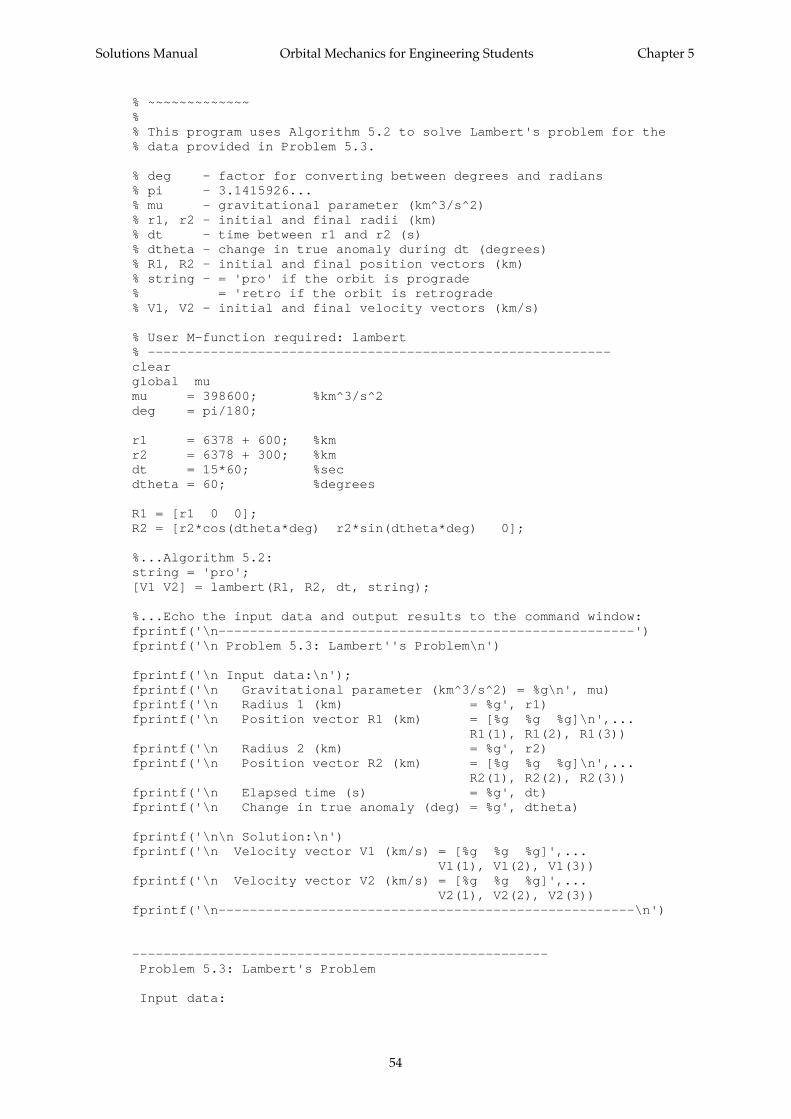
Solutions Manual Orbital Mechanics for Engineering Students Chapter 5
54
% ~~~~~~~~~~~~~%% This program uses Algorithm 5.2 to solve Lambert's problem for the% data provided in Problem 5.3.
% deg - factor for converting between degrees and radians% pi - 3.1415926...% mu - gravitational parameter (km^3/s^2)% r1, r2 - initial and final radii (km)% dt - time between r1 and r2 (s)% dtheta - change in true anomaly during dt (degrees)% R1, R2 - initial and final position vectors (km)% string - = 'pro' if the orbit is prograde% = 'retro if the orbit is retrograde% V1, V2 - initial and final velocity vectors (km/s)
% User M-function required: lambert% -----------------------------------------------------------clearglobal mumu = 398600; %km^3/s^2deg = pi/180;
r1 = 6378 + 600; %kmr2 = 6378 + 300; %kmdt = 15*60; %secdtheta = 60; %degrees
R1 = [r1 0 0];R2 = [r2*cos(dtheta*deg) r2*sin(dtheta*deg) 0];
%...Algorithm 5.2:string = 'pro';[V1 V2] = lambert(R1, R2, dt, string);
%...Echo the input data and output results to the command window:fprintf('\n-----------------------------------------------------')fprintf('\n Problem 5.3: Lambert''s Problem\n')
fprintf('\n Input data:\n');fprintf('\n Gravitational parameter (km^3/s^2) = %g\n', mu)fprintf('\n Radius 1 (km) = %g', r1)fprintf('\n Position vector R1 (km) = [%g %g %g]\n',... R1(1), R1(2), R1(3))fprintf('\n Radius 2 (km) = %g', r2)fprintf('\n Position vector R2 (km) = [%g %g %g]\n',... R2(1), R2(2), R2(3))fprintf('\n Elapsed time (s) = %g', dt)fprintf('\n Change in true anomaly (deg) = %g', dtheta)
fprintf('\n\n Solution:\n')fprintf('\n Velocity vector V1 (km/s) = [%g %g %g]',... V1(1), V1(2), V1(3))fprintf('\n Velocity vector V2 (km/s) = [%g %g %g]',... V2(1), V2(2), V2(3))fprintf('\n-----------------------------------------------------\n')
----------------------------------------------------- Problem 5.3: Lambert's Problem
Input data:

Solutions Manual Orbital Mechanics for Engineering Students Chapter 5
55
Gravitational parameter (km^3/s^2) = 398600
Radius 1 (km) = 6978 Position vector R1 (km) = [6978 0 0]
Radius 2 (km) = 6678 Position vector R2 (km) = [3339 5783.32 0]
Elapsed time (s) = 900 Change in true anomaly (deg) = 60
Solution:
Velocity vector V1 (km/s) = [-0.544135 7.68498 0] Velocity vector V2 (km/s) = [-6.98129 3.96849 0]-----------------------------------------------------
To find the perigee altitude, we need the orbital elements. The following MATLAB script uses
r i1 6978= ( )ˆ km and v i j1 km/s= − + ( )0 544135 7 68498. ˆ . ˆ from above to compute the orbital elementsby means of Algorithm 4.1, which is implemented as the M-function coe_from_sv in Appendix D.8.The output to the MATLAB Command Window is listed afterwards.
% ~~~~~~~~~~~~~~~~~~~~~~~~~~~~~~~~~~~~~~~~~~~~~~~~~~~~~~~~~~~~~~~~~~~~% Problem_5_03b% ~~~~~~~~~~~~%% This program employs Algorithm 4.1 to obtain the orbital% elements from the state vector found from the solution% of Lambert's problem using the data given in Problem 5.3.%% pi - 3.1415926...% deg - factor for converting between degrees and radians% mu - gravitational parameter (km^3/s^2)% r - position vector (km) in the geocentric equatorial frame% v - velocity vector (km/s) in the geocentric equatorial frame% coe - orbital elements [h e RA incl w TA a]% where h = angular momentum (km^2/s)% e = eccentricity% RA = right ascension of the ascending node (rad)% incl = orbit inclination (rad)% w = argument of perigee (rad)% TA = true anomaly (rad)% a = semimajor axis (km)% T - Period of an elliptic orbit (s)%% User M-function required: coe_from_sv% --------------------------------------------------------------------
clearglobal mudeg = pi/180;mu = 398600;
%...Data declaration for Problem 5.3:r = [6978 0 0];v = [-0.544135 7.68498 0];%...
%...Algorithm 4.1:coe = coe_from_sv(r,v);
%...Echo the input data and output results to the command window:
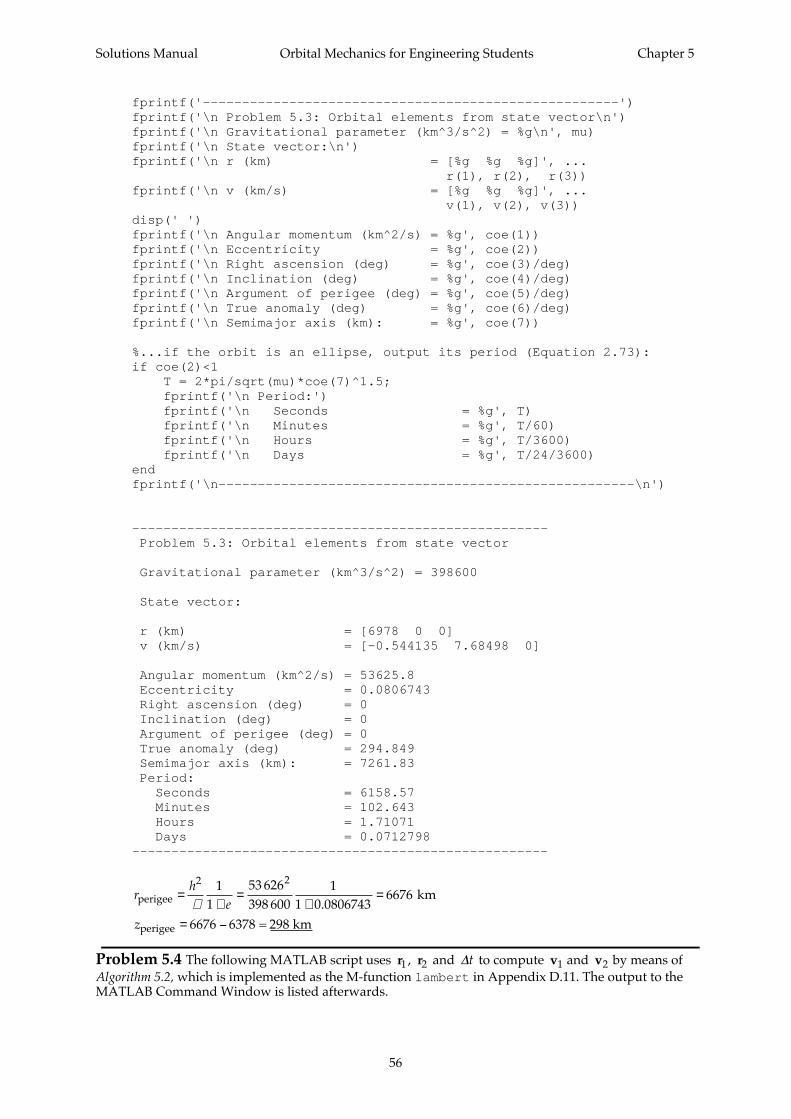
Solutions Manual Orbital Mechanics for Engineering Students Chapter 5
56
fprintf('-----------------------------------------------------')fprintf('\n Problem 5.3: Orbital elements from state vector\n')fprintf('\n Gravitational parameter (km^3/s^2) = %g\n', mu)fprintf('\n State vector:\n')fprintf('\n r (km) = [%g %g %g]', ... r(1), r(2), r(3))fprintf('\n v (km/s) = [%g %g %g]', ... v(1), v(2), v(3))disp(' ')fprintf('\n Angular momentum (km^2/s) = %g', coe(1))fprintf('\n Eccentricity = %g', coe(2))fprintf('\n Right ascension (deg) = %g', coe(3)/deg)fprintf('\n Inclination (deg) = %g', coe(4)/deg)fprintf('\n Argument of perigee (deg) = %g', coe(5)/deg)fprintf('\n True anomaly (deg) = %g', coe(6)/deg)fprintf('\n Semimajor axis (km): = %g', coe(7))
%...if the orbit is an ellipse, output its period (Equation 2.73):if coe(2)<1 T = 2*pi/sqrt(mu)*coe(7)^1.5; fprintf('\n Period:') fprintf('\n Seconds = %g', T) fprintf('\n Minutes = %g', T/60) fprintf('\n Hours = %g', T/3600) fprintf('\n Days = %g', T/24/3600)endfprintf('\n-----------------------------------------------------\n')
----------------------------------------------------- Problem 5.3: Orbital elements from state vector
Gravitational parameter (km^3/s^2) = 398600
State vector:
r (km) = [6978 0 0] v (km/s) = [-0.544135 7.68498 0]
Angular momentum (km^2/s) = 53625.8 Eccentricity = 0.0806743 Right ascension (deg) = 0 Inclination (deg) = 0 Argument of perigee (deg) = 0 True anomaly (deg) = 294.849 Semimajor axis (km): = 7261.83 Period: Seconds = 6158.57 Minutes = 102.643 Hours = 1.71071 Days = 0.0712798-----------------------------------------------------
rh
e
z
perigee
perigee
km
6378 = 298 km
=+
=+
=
= −
2 211
53 626398 600
11 0 0806743
6676
6676µ .
Problem 5.4 The following MATLAB script uses r1 , r2 and ∆t to compute v1 and v2 by means ofAlgorithm 5.2, which is implemented as the M-function lambert in Appendix D.11. The output to theMATLAB Command Window is listed afterwards.
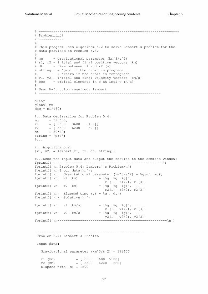
Solutions Manual Orbital Mechanics for Engineering Students Chapter 5
57
% ~~~~~~~~~~~~~~~~~~~~~~~~~~~~~~~~~~~~~~~~~~~~~~~~~~~~~~~~~~~~~~~~~~~~% Problem_5_04% ~~~~~~~~~~~~%% This program uses Algorithm 5.2 to solve Lambert's problem for the% data provided in Problem 5.4.%% mu - gravitational parameter (km^3/s^2)% r1, r2 - initial and final position vectors (km)% dt - time between r1 and r2 (s)% string - = 'pro' if the orbit is prograde% = 'retro if the orbit is retrograde% v1, v2 - initial and final velocity vectors (km/s)% coe - orbital elements [h e RA incl w TA a]%% User M-function required: lambert% -----------------------------------------------------------
clearglobal mudeg = pi/180;
%...Data declaration for Problem 5.4:mu = 398600;r1 = [-3600 3600 5100];r2 = [-5500 -6240 -520];dt = 30*60;string = 'pro';%...
%...Algorithm 5.2:[v1, v2] = lambert(r1, r2, dt, string);
%...Echo the input data and output the results to the command window:fprintf('-----------------------------------------------------')fprintf('\n Problem 5.4: Lambert''s Problem\n')fprintf('\n Input data:\n');fprintf('\n Gravitational parameter (km^3/s^2) = %g\n', mu);fprintf('\n r1 (km) = [%g %g %g]', ... r1(1), r1(2), r1(3))fprintf('\n r2 (km) = [%g %g %g]', ... r2(1), r2(2), r2(3))fprintf('\n Elapsed time (s) = %g', dt);fprintf('\n\n Solution:\n')
fprintf('\n v1 (km/s) = [%g %g %g]', ... v1(1), v1(2), v1(3))fprintf('\n v2 (km/s) = [%g %g %g]', ... v2(1), v2(2), v2(3))fprintf('\n-----------------------------------------------------\n')
----------------------------------------------------- Problem 5.4: Lambert's Problem
Input data:
Gravitational parameter (km^3/s^2) = 398600
r1 (km) = [-3600 3600 5100] r2 (km) = [-5500 -6240 -520] Elapsed time (s) = 1800
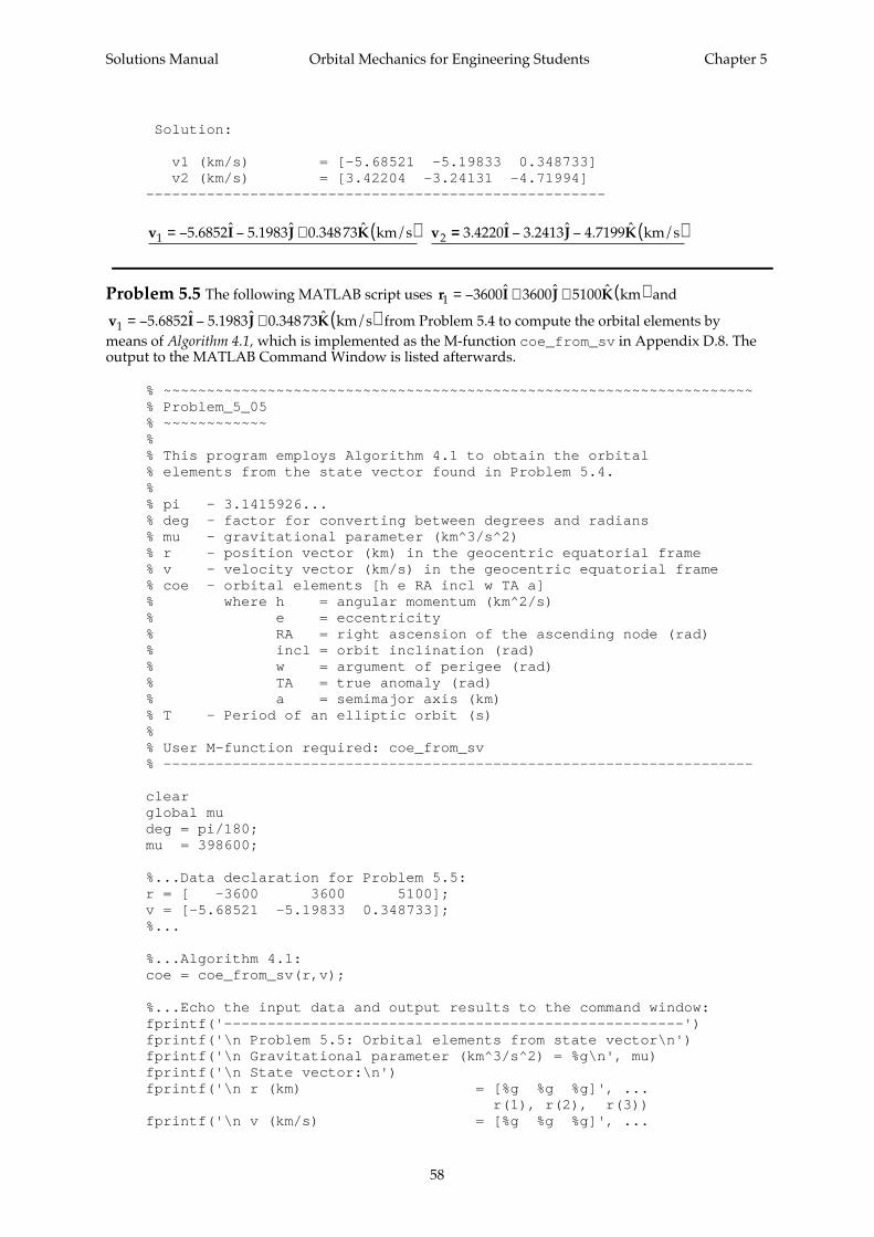
Solutions Manual Orbital Mechanics for Engineering Students Chapter 5
58
Solution:
v1 (km/s) = [-5.68521 -5.19833 0.348733] v2 (km/s) = [3.42204 -3.24131 -4.71994]-----------------------------------------------------
v I J K v1 km/s= − − + ( )5 6852 5 1983 0 34873 2. ˆ . ˆ . ˆ == − − ( )3 4220 3 2413 4 7199. ˆ . ˆ . ˆI J K km/s
Problem 5.5 The following MATLAB script uses r I J K1 km= − + + ( )3600 3600 5100ˆ ˆ ˆ and
v I J K1 km/s= − − + ( )5 6852 5 1983 0 34873. ˆ . ˆ . ˆ from Problem 5.4 to compute the orbital elements bymeans of Algorithm 4.1, which is implemented as the M-function coe_from_sv in Appendix D.8. Theoutput to the MATLAB Command Window is listed afterwards.
% ~~~~~~~~~~~~~~~~~~~~~~~~~~~~~~~~~~~~~~~~~~~~~~~~~~~~~~~~~~~~~~~~~~~~% Problem_5_05% ~~~~~~~~~~~~%% This program employs Algorithm 4.1 to obtain the orbital% elements from the state vector found in Problem 5.4.%% pi - 3.1415926...% deg - factor for converting between degrees and radians% mu - gravitational parameter (km^3/s^2)% r - position vector (km) in the geocentric equatorial frame% v - velocity vector (km/s) in the geocentric equatorial frame% coe - orbital elements [h e RA incl w TA a]% where h = angular momentum (km^2/s)% e = eccentricity% RA = right ascension of the ascending node (rad)% incl = orbit inclination (rad)% w = argument of perigee (rad)% TA = true anomaly (rad)% a = semimajor axis (km)% T - Period of an elliptic orbit (s)%% User M-function required: coe_from_sv% --------------------------------------------------------------------
clearglobal mudeg = pi/180;mu = 398600;
%...Data declaration for Problem 5.5:r = [ -3600 3600 5100];v = [-5.68521 -5.19833 0.348733];%...
%...Algorithm 4.1:coe = coe_from_sv(r,v);
%...Echo the input data and output results to the command window:fprintf('-----------------------------------------------------')fprintf('\n Problem 5.5: Orbital elements from state vector\n')fprintf('\n Gravitational parameter (km^3/s^2) = %g\n', mu)fprintf('\n State vector:\n')fprintf('\n r (km) = [%g %g %g]', ... r(1), r(2), r(3))fprintf('\n v (km/s) = [%g %g %g]', ...
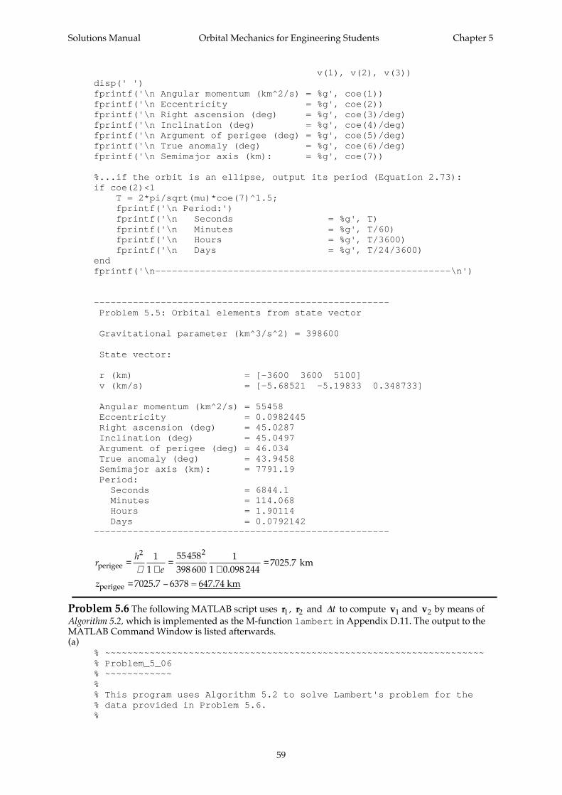
Solutions Manual Orbital Mechanics for Engineering Students Chapter 5
59
v(1), v(2), v(3))disp(' ')fprintf('\n Angular momentum (km^2/s) = %g', coe(1))fprintf('\n Eccentricity = %g', coe(2))fprintf('\n Right ascension (deg) = %g', coe(3)/deg)fprintf('\n Inclination (deg) = %g', coe(4)/deg)fprintf('\n Argument of perigee (deg) = %g', coe(5)/deg)fprintf('\n True anomaly (deg) = %g', coe(6)/deg)fprintf('\n Semimajor axis (km): = %g', coe(7))
%...if the orbit is an ellipse, output its period (Equation 2.73):if coe(2)<1 T = 2*pi/sqrt(mu)*coe(7)^1.5; fprintf('\n Period:') fprintf('\n Seconds = %g', T) fprintf('\n Minutes = %g', T/60) fprintf('\n Hours = %g', T/3600) fprintf('\n Days = %g', T/24/3600)endfprintf('\n-----------------------------------------------------\n')
----------------------------------------------------- Problem 5.5: Orbital elements from state vector
Gravitational parameter (km^3/s^2) = 398600
State vector:
r (km) = [-3600 3600 5100] v (km/s) = [-5.68521 -5.19833 0.348733]
Angular momentum (km^2/s) = 55458 Eccentricity = 0.0982445 Right ascension (deg) = 45.0287 Inclination (deg) = 45.0497 Argument of perigee (deg) = 46.034 True anomaly (deg) = 43.9458 Semimajor axis (km): = 7791.19 Period: Seconds = 6844.1 Minutes = 114.068 Hours = 1.90114 Days = 0.0792142-----------------------------------------------------
rh
e
z
perigee
perigee
km
6378 = 647.74 km
=+
=+
=
= −
2 211
55458398 600
11 0 098 244
7025 7
7025 7µ .
.
.
Problem 5.6 The following MATLAB script uses r1 , r2 and ∆t to compute v1 and v2 by means ofAlgorithm 5.2, which is implemented as the M-function lambert in Appendix D.11. The output to theMATLAB Command Window is listed afterwards.(a)
% ~~~~~~~~~~~~~~~~~~~~~~~~~~~~~~~~~~~~~~~~~~~~~~~~~~~~~~~~~~~~~~~~~~~~% Problem_5_06% ~~~~~~~~~~~~%% This program uses Algorithm 5.2 to solve Lambert's problem for the% data provided in Problem 5.6.%
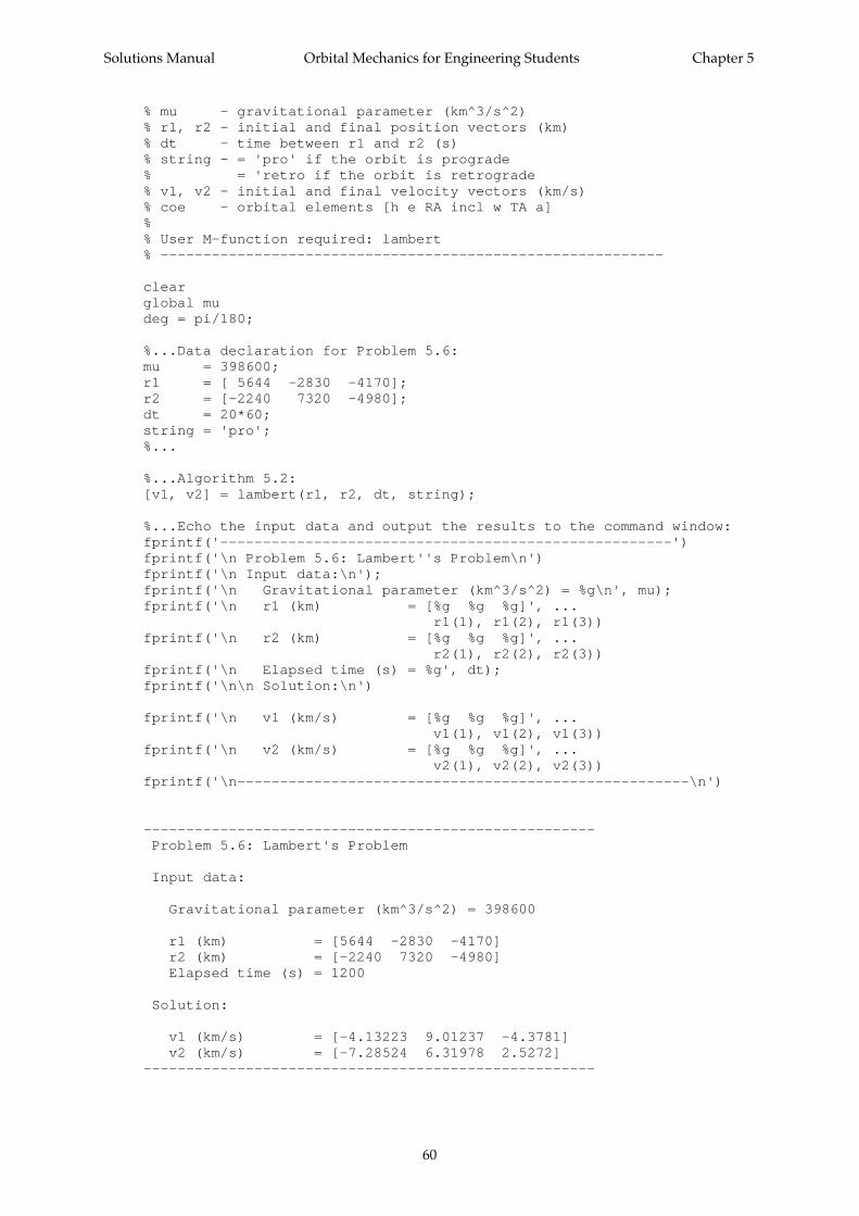
Solutions Manual Orbital Mechanics for Engineering Students Chapter 5
60
% mu - gravitational parameter (km^3/s^2)% r1, r2 - initial and final position vectors (km)% dt - time between r1 and r2 (s)% string - = 'pro' if the orbit is prograde% = 'retro if the orbit is retrograde% v1, v2 - initial and final velocity vectors (km/s)% coe - orbital elements [h e RA incl w TA a]%% User M-function required: lambert% -----------------------------------------------------------
clearglobal mudeg = pi/180;
%...Data declaration for Problem 5.6:mu = 398600;r1 = [ 5644 -2830 -4170];r2 = [-2240 7320 -4980];dt = 20*60;string = 'pro';%...
%...Algorithm 5.2:[v1, v2] = lambert(r1, r2, dt, string);
%...Echo the input data and output the results to the command window:fprintf('-----------------------------------------------------')fprintf('\n Problem 5.6: Lambert''s Problem\n')fprintf('\n Input data:\n');fprintf('\n Gravitational parameter (km^3/s^2) = %g\n', mu);fprintf('\n r1 (km) = [%g %g %g]', ... r1(1), r1(2), r1(3))fprintf('\n r2 (km) = [%g %g %g]', ... r2(1), r2(2), r2(3))fprintf('\n Elapsed time (s) = %g', dt);fprintf('\n\n Solution:\n')
fprintf('\n v1 (km/s) = [%g %g %g]', ... v1(1), v1(2), v1(3))fprintf('\n v2 (km/s) = [%g %g %g]', ... v2(1), v2(2), v2(3))fprintf('\n-----------------------------------------------------\n')
----------------------------------------------------- Problem 5.6: Lambert's Problem
Input data:
Gravitational parameter (km^3/s^2) = 398600
r1 (km) = [5644 -2830 -4170] r2 (km) = [-2240 7320 -4980] Elapsed time (s) = 1200
Solution:
v1 (km/s) = [-4.13223 9.01237 -4.3781] v2 (km/s) = [-7.28524 6.31978 2.5272]-----------------------------------------------------
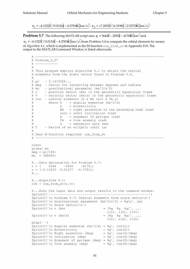
Solutions Manual Orbital Mechanics for Engineering Students Chapter 5
61
v I J K v1 km/s= − + − ( ) =4 1322 9 0124 4 3781 2. ˆ . ˆ . ˆ −− + + ( )7 2852 6 3198 2 5272. ˆ . ˆ . ˆI J K km/s
Problem 5.7 The following MATLAB script uses r I J K1 km= − − ( )5644 2830 4170ˆ ˆ ˆ and
v I J K1 km/s= − + − ( )4 1322 9 0124 4 3781. ˆ . ˆ . ˆ from Problem 5.4 to compute the orbital elements by meansof Algorithm 4.1, which is implemented as the M-function coe_from_sv in Appendix D.8. Theoutput to the MATLAB Command Window is listed afterwards.
% ~~~~~~~~~~~~~~~~~~~~~~~~~~~~~~~~~~~~~~~~~~~~~~~~~~~~~~~~~~~~~~~~~~~~% Problem_5_07% ~~~~~~~~~~~~%% This program employs Algorithm 4.1 to obtain the orbital% elements from the state vector found in Problem 5.6.%% pi - 3.1415926...% deg - factor for converting between degrees and radians% mu - gravitational parameter (km^3/s^2)% r - position vector (km) in the geocentric equatorial frame% v - velocity vector (km/s) in the geocentric equatorial frame% coe - orbital elements [h e RA incl w TA a]% where h = angular momentum (km^2/s)% e = eccentricity% RA = right ascension of the ascending node (rad)% incl = orbit inclination (rad)% w = argument of perigee (rad)% TA = true anomaly (rad)% a = semimajor axis (km)% T - Period of an elliptic orbit (s)%% User M-function required: coe_from_sv% --------------------------------------------------------------------
clearglobal mudeg = pi/180;mu = 398600;
%...Data declaration for Problem 5.7:r = [ 5644 -2830 -4170];v = [-4.13223 9.01237 -4.3781];%...
%...Algorithm 4.1:coe = coe_from_sv(r,v);
%...Echo the input data and output results to the command window:fprintf('-----------------------------------------------------')fprintf('\n Problem 5.7: Orbital elements from state vector\n')fprintf('\n Gravitational parameter (km^3/s^2) = %g\n', mu)fprintf('\n State vector:\n')fprintf('\n r (km) = [%g %g %g]', ... r(1), r(2), r(3))fprintf('\n v (km/s) = [%g %g %g]', ... v(1), v(2), v(3))disp(' ')fprintf('\n Angular momentum (km^2/s) = %g', coe(1))fprintf('\n Eccentricity = %g', coe(2))fprintf('\n Right ascension (deg) = %g', coe(3)/deg)fprintf('\n Inclination (deg) = %g', coe(4)/deg)fprintf('\n Argument of perigee (deg) = %g', coe(5)/deg)fprintf('\n True anomaly (deg) = %g', coe(6)/deg)
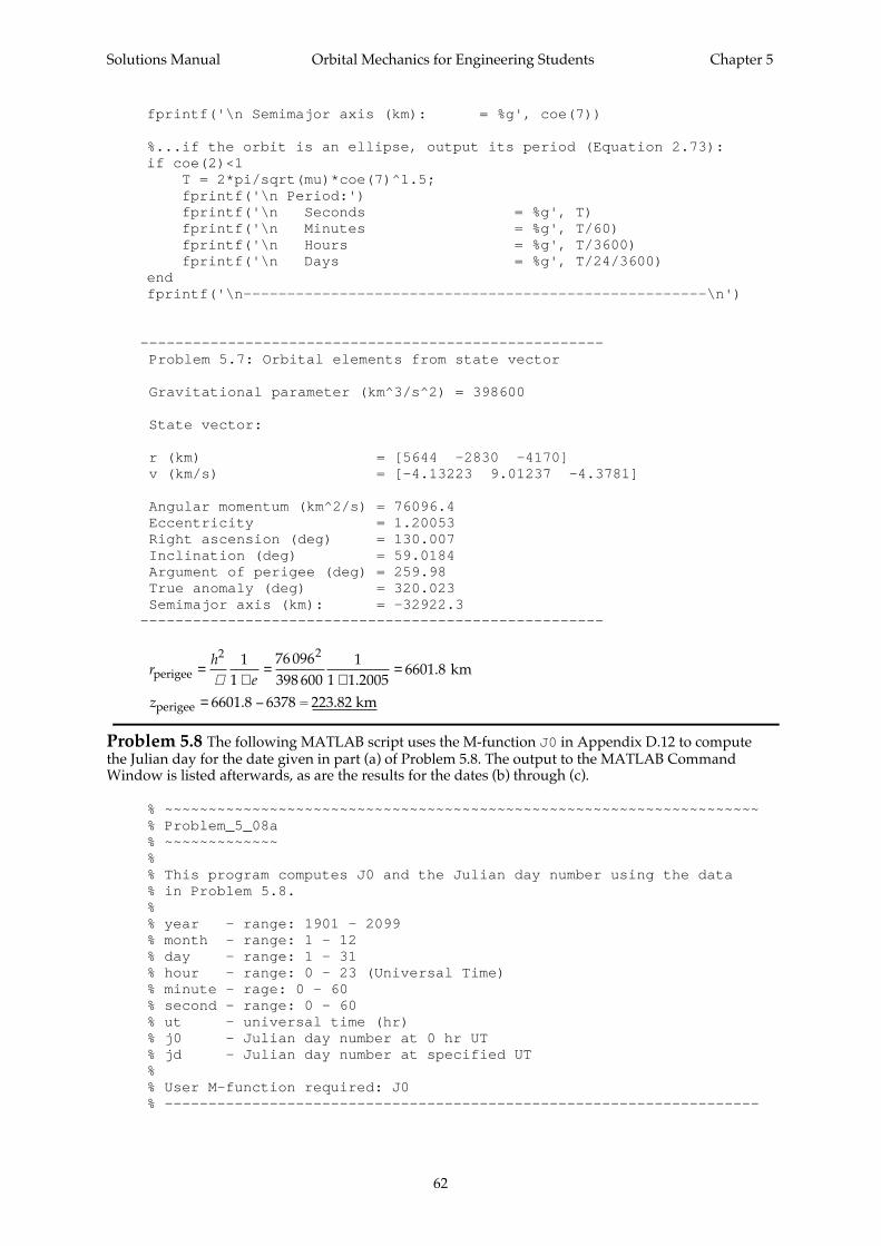
Solutions Manual Orbital Mechanics for Engineering Students Chapter 5
62
fprintf('\n Semimajor axis (km): = %g', coe(7))
%...if the orbit is an ellipse, output its period (Equation 2.73):if coe(2)<1 T = 2*pi/sqrt(mu)*coe(7)^1.5; fprintf('\n Period:') fprintf('\n Seconds = %g', T) fprintf('\n Minutes = %g', T/60) fprintf('\n Hours = %g', T/3600) fprintf('\n Days = %g', T/24/3600)endfprintf('\n-----------------------------------------------------\n')
----------------------------------------------------- Problem 5.7: Orbital elements from state vector
Gravitational parameter (km^3/s^2) = 398600
State vector:
r (km) = [5644 -2830 -4170] v (km/s) = [-4.13223 9.01237 -4.3781]
Angular momentum (km^2/s) = 76096.4 Eccentricity = 1.20053 Right ascension (deg) = 130.007 Inclination (deg) = 59.0184 Argument of perigee (deg) = 259.98 True anomaly (deg) = 320.023 Semimajor axis (km): = -32922.3-----------------------------------------------------
rh
e
z
perigee
perigee
km
6378 = 223.82 km
=+
=+
=
= −
2 211
76 096398 600
11 1 2005
6601 8
6601 8µ .
.
.
Problem 5.8 The following MATLAB script uses the M-function J0 in Appendix D.12 to computethe Julian day for the date given in part (a) of Problem 5.8. The output to the MATLAB CommandWindow is listed afterwards, as are the results for the dates (b) through (c).
% ~~~~~~~~~~~~~~~~~~~~~~~~~~~~~~~~~~~~~~~~~~~~~~~~~~~~~~~~~~~~~~~~~~~~% Problem_5_08a% ~~~~~~~~~~~~~%% This program computes J0 and the Julian day number using the data% in Problem 5.8.%% year - range: 1901 - 2099% month - range: 1 - 12% day - range: 1 - 31% hour - range: 0 - 23 (Universal Time)% minute - rage: 0 - 60% second - range: 0 - 60% ut - universal time (hr)% j0 - Julian day number at 0 hr UT% jd - Julian day number at specified UT%% User M-function required: J0% --------------------------------------------------------------------
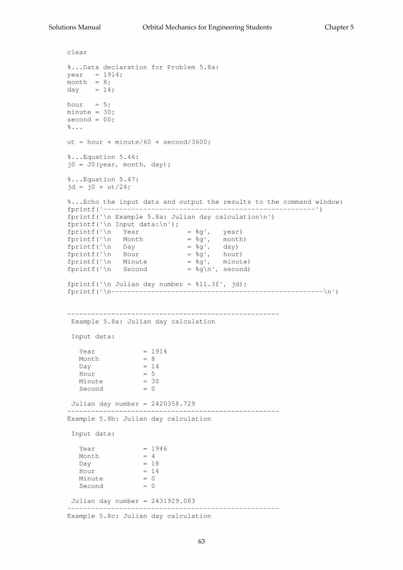
Solutions Manual Orbital Mechanics for Engineering Students Chapter 5
63
clear
%...Data declaration for Problem 5.8a:year = 1914;month = 8;day = 14;
hour = 5;minute = 30;second = 00;%...
ut = hour + minute/60 + second/3600;
%...Equation 5.46:j0 = J0(year, month, day);
%...Equation 5.47:jd = j0 + ut/24;
%...Echo the input data and output the results to the command window:fprintf('-----------------------------------------------------')fprintf('\n Example 5.8a: Julian day calculation\n')fprintf('\n Input data:\n');fprintf('\n Year = %g', year)fprintf('\n Month = %g', month)fprintf('\n Day = %g', day)fprintf('\n Hour = %g', hour)fprintf('\n Minute = %g', minute)fprintf('\n Second = %g\n', second)
fprintf('\n Julian day number = %11.3f', jd);fprintf('\n-----------------------------------------------------\n')
----------------------------------------------------- Example 5.8a: Julian day calculation
Input data:
Year = 1914 Month = 8 Day = 14 Hour = 5 Minute = 30 Second = 0
Julian day number = 2420358.729-----------------------------------------------------Example 5.8b: Julian day calculation
Input data:
Year = 1946 Month = 4 Day = 18 Hour = 14 Minute = 0 Second = 0
Julian day number = 2431929.083-----------------------------------------------------Example 5.8c: Julian day calculation
Solutions Manual Orbital Mechanics for Engineering Students Chapter 5
64
Input data:
Year = 2010 Month = 9 Day = 1 Hour = 0 Minute = 0 Second = 0
Julian day number = 2455440.500-----------------------------------------------------Example 5.8d: Julian day calculation
Input data:
Year = 2007 Month = 10 Day = 16 Hour = 12 Minute = 0 Second = 0
Julian day number = 2454390.000-----------------------------------------------------
Problem 5.9 This is similar to Example 5.5. The MATLAB script listed in the solution to Problem5.8 can be used to obtain the Julian day numbers.
Problem 5.10 The following MATLAB script uses Algorithm 5.3, which is implemented in MATLABby the M-function LST in Appendix D.13, to compute the local sidereal time for the data given in part(a) of Problem 5.10. The output to the MATLAB Command Window is listed afterwards, as are theresults for the data in (b) through (e).
% ~~~~~~~~~~~~~~~~~~~~~~~~~~~~~~~~~~~~~~~~~~~~~~~~~~~~~~~~~~~~~~~~~~~~% Problem_5_10a% ~~~~~~~~~~~~~%% This program uses Algorithm 5.3 to obtain the local sidereal% time from the data provided in Problem 5.10.%% lst - local sidereal time (degrees)% EL - east longitude of the site (west longitude is negative):% degrees (0 - 360)% minutes (0 - 60)% seconds (0 - 60)% WL - west longitude% year - range: 1901 - 2099% month - range: 1 - 12% day - range: 1 - 31% ut - universal time% hour (0 - 23)% minute (0 - 60)% second (0 - 60)%% User M-function required: LST% --------------------------------------------------------------------
clear
%...Data declaration for Problem 5.10a:
Solutions Manual Orbital Mechanics for Engineering Students Chapter 5
65
% East longitude:degrees = 18;minutes = 3;seconds = 0;
% Date:year = 2008;month = 1;day = 1;
% Universal time:hour = 12;minute = 0;second = 0;
%...
%...Convert negative (west) longitude to east longitude:if degrees < 0 degrees = degrees + 360;end
%...Express the longitudes as decimal numbers:EL = degrees + minutes/60 + seconds/3600;WL = 360 - EL;
%...Express universal time as a decimal number:ut = hour + minute/60 + second/3600;
%...Algorithm 5.3:lst = LST(year, month, day, ut, EL);
%...Echo the input data and output the results to the command window:fprintf('-----------------------------------------------------')fprintf('\n Problem 5.10a: Local sidereal time calculation\n')fprintf('\n Input data:\n');fprintf('\n Year = %g', year)fprintf('\n Month = %g', month)fprintf('\n Day = %g', day)fprintf('\n UT (hr) = %g', ut)fprintf('\n West Longitude (deg) = %g', WL)fprintf('\n East Longitude (deg) = %g', EL)fprintf('\n\n');
fprintf(' Solution:')fprintf('\n');fprintf('\n Local Sidereal Time (deg) = %g', lst)fprintf('\n Local Sidereal Time (hr) = %g', lst/15)fprintf('\n-----------------------------------------------------\n')
----------------------------------------------------- Problem 5.10a: Local sidereal time calculation
Input data:
Year = 2008 Month = 1 Day = 1 UT (hr) = 12 West Longitude (deg) = 341.95 East Longitude (deg) = 18.05
Solutions Manual Orbital Mechanics for Engineering Students Chapter 5
66
Solution:
Local Sidereal Time (deg) = 298.572 Local Sidereal Time (hr) = 19.9048----------------------------------------------------- Problem 5.10b: Local sidereal time calculation
Input data:
Year = 2007 Month = 12 Day = 21 UT (hr) = 10 West Longitude (deg) = 215.033 East Longitude (deg) = 144.967
Solution:
Local Sidereal Time (deg) = 24.5646 Local Sidereal Time (hr) = 1.63764----------------------------------------------------- Problem 5.10c: Local sidereal time calculation
Input data:
Year = 2005 Month = 7 Day = 4 UT (hr) = 20 West Longitude (deg) = 118.25 East Longitude (deg) = 241.75
Solution:
Local Sidereal Time (deg) = 104.676 Local Sidereal Time (hr) = 6.9784----------------------------------------------------- Problem 5.10d: Local sidereal time calculation
Input data:
Year = 2006 Month = 2 Day = 15 UT (hr) = 3 West Longitude (deg) = 43.1 East Longitude (deg) = 316.9
Solution:
Local Sidereal Time (deg) = 146.884 Local Sidereal Time (hr) = 9.79228----------------------------------------------------- Problem 5.10e: Local sidereal time calculation
Input data:
Year = 2006 Month = 3 Day = 21 UT (hr) = 8 West Longitude (deg) = 228.067 East Longitude (deg) = 131.933
Solutions Manual Orbital Mechanics for Engineering Students Chapter 5
67
Solution:
Local Sidereal Time (deg) = 70.6348 Local Sidereal Time (hr) = 4.70899-----------------------------------------------------
Problem 5.11. θ φ= ° = ° = ° = °117 51 28 68Α a .
From Equation 5.83a,
δ φ φ
δ
= +( )= ° ° ° + ° °( )
= °
− −sin cos cos cos sin sin sin cos cos cos sin sin.
1 1 51 28 68 117 6868 235
A a a
From Equation 5.83b, since A < °180 ,
ha A a
= ° −−
= ° −° ° − ° ° °
°
= °
−
−
360
36051 68 51 28 68
68 235331 69
1
1
coscos sin sin cos cos
cos
coscos sin sin cos cos
cos ..
φ φδ
From Equation 5.83c
α θ= − = ° − ° = −h 117 331 69 214 69. .
Placing this within the range 0 360≤ ≤ °θ ,
α = °145 31.
Problem 5.12 The following MATLAB script uses Algorithm 5.4, which is implemented in MATLABby the M-function rv_from_observe in Appendix D.14, to compute the state vector of a spaceobject from the data given in Problem 5.12. The output to the MATLAB Command Window is listedafterwards.
% ~~~~~~~~~~~~~~~~~~~~~~~~~~~~~~~~~~~~~~~~~~~~~~~~~~~~~~~~~~~~~~~~~~~~% Problem_5_12% ~~~~~~~~~~~~%% This program uses Algorithm 5.4 to obtain the state% vector from the observational data provided in Problem 5.12.%% deg - conversion factor between degrees and radians% pi - 3.1415926...% mu - gravitational parameter (km^3/s^2)
% Re - equatorial radius of the earth (km)% f - earth's flattening factor% wE - angular velocity of the earth (rad/s)% omega - earth's angular velocity vector (rad/s) in the% geocentric equatorial frame
% rho - slant range of object (km)% rhodot - range rate (km/s)% A - azimuth (deg) of object relative to observation site% Adot - time rate of change of azimuth (deg/s)% a - elevation angle (deg) of object relative to observationsite
Solutions Manual Orbital Mechanics for Engineering Students Chapter 5
68
% adot - time rate of change of elevation angle (degrees/s)
% theta - local sidereal time (deg) of tracking site% phi - geodetic latitude (deg) of site% H - elevation of site (km)
% r - geocentric equatorial position vector of object (km)% v - geocentric equatorial velocity vector of object (km)
% coe - orbital elements [h e RA incl w TA a]% where% h = angular momentum (km^2/s)% e = eccentricity% RA = right ascension of the ascending node (rad)% incl = inclination of the orbit (rad)% w = argument of perigee (rad)% TA = true anomaly (rad)% a = semimajor axis (km)% rp - perigee radius (km)% T - period of elliptical orbit (s)%% User M-function required: rv_from_observe% --------------------------------------------------------------------
clearglobal f Re wE mu
deg = pi/180;f = 0.0033528;Re = 6378;wE = 7.2921e-5;mu = 398600;
%...Data declaration for Problem 5.12:rho = 988;rhodot = 4.86;A = 36;Adot = 0.59;a = 36.6;adot = -0.263;theta = 40;phi = 35;H = 0;%...
%...Algorithm 5.4:[r,v] = rv_from_observe(rho, rhodot, A, Adot, a, adot, theta, phi, H);
%...Echo the input data and output the solution to% the command window:fprintf('-----------------------------------------------------')fprintf('\n Problem 5.12')fprintf('\n\n Input data:\n');fprintf('\n Slant range (km) = %g', rho);fprintf('\n Slant range rate (km/s) = %g', rhodot);fprintf('\n Azimuth (deg) = %g', A);fprintf('\n Azimuth rate (deg/s) = %g', Adot);fprintf('\n Elevation (deg) = %g', a);fprintf('\n Elevation rate (deg/s) = %g', adot);fprintf('\n Local sidereal time (deg) = %g', theta);fprintf('\n Latitude (deg) = %g', phi);fprintf('\n Altitude above sea level (km) = %g', H);fprintf('\n\n');

Solutions Manual Orbital Mechanics for Engineering Students Chapter 5
69
fprintf(' Solution:')
fprintf('\n\n State vector:\n');fprintf('\n r (km) = [%g, %g, %g]', ... r(1), r(2), r(3));fprintf('\n v (km/s) = [%g, %g, %g]', ... v(1), v(2), v(3));fprintf('\n-----------------------------------------------------\n')
----------------------------------------------------- Problem 5.12
Input data:
Slant range (km) = 988 Slant range rate (km/s) = 4.86 Azimuth (deg) = 36 Azimuth rate (deg/s) = 0.59 Elevation (deg) = 36.6 Elevation rate (deg/s) = -0.263 Local sidereal time (deg) = 40 Latitude (deg) = 35 Altitude above sea level (km) = 0
Solution:
State vector:
r (km) = [3794.66, 3792.71, 4501.31] v (km/s) = [-7.72483, 7.72134, 0.0186586]-----------------------------------------------------
r I J K v= + + ( ) = −3794 7 3792 7 4501 3 7 7. ˆ . ˆ . ˆ .km 2248 7 72134 0 018 659ˆ . ˆ . ˆI J K+ + ( )km/s
Problem 5.13 The following MATLAB script uses the state vector found in Problem 5.12 tocompute the orbital elements by means of Algorithm 4.1, which is implemented as the M-functioncoe_from_sv in Appendix D.8. The output to the MATLAB Command Window is listed afterwards.
% ~~~~~~~~~~~~~~~~~~~~~~~~~~~~~~~~~~~~~~~~~~~~~~~~~~~~~~~~~~~~~~~~~~~~% Problem_5_13% ~~~~~~~~~~~~%% This program employs Algorithm 4.1 to obtain the orbital% elements from the state vector found in Problem 5.12.%% pi - 3.1415926...% deg - factor for converting between degrees and radians% mu - gravitational parameter (km^3/s^2)% r - position vector (km) in the geocentric equatorial frame% v - velocity vector (km/s) in the geocentric equatorial frame% coe - orbital elements [h e RA incl w TA a]% where h = angular momentum (km^2/s)% e = eccentricity% RA = right ascension of the ascending node (rad)% incl = orbit inclination (rad)% w = argument of perigee (rad)% TA = true anomaly (rad)% a = semimajor axis (km)% T - Period of an elliptic orbit (s)%
Solutions Manual Orbital Mechanics for Engineering Students Chapter 5
70
% User M-function required: coe_from_sv% --------------------------------------------------------------------
clearglobal mudeg = pi/180;mu = 398600;
%...Data declaration for Problem 5.13:r = [ 3794.66, 3792.71, 4501.31];v = [-7.72483, 7.72134, 0.0186586];%...
%...Algorithm 4.1:coe = coe_from_sv(r,v);
%...Echo the input data and output results to the command window:fprintf('-----------------------------------------------------')fprintf('\n Problem 5.13: Orbital elements from state vector\n')fprintf('\n Gravitational parameter (km^3/s^2) = %g\n', mu)fprintf('\n State vector:\n')fprintf('\n r (km) = [%g %g %g]', ... r(1), r(2), r(3))fprintf('\n v (km/s) = [%g %g %g]', ... v(1), v(2), v(3))disp(' ')fprintf('\n Angular momentum (km^2/s) = %g', coe(1))fprintf('\n Eccentricity = %g', coe(2))fprintf('\n Right ascension (deg) = %g', coe(3)/deg)fprintf('\n Inclination (deg) = %g', coe(4)/deg)fprintf('\n Argument of perigee (deg) = %g', coe(5)/deg)fprintf('\n True anomaly (deg) = %g', coe(6)/deg)fprintf('\n Semimajor axis (km): = %g', coe(7))
%...if the orbit is an ellipse, output its period (Equation 2.73):if coe(2)<1 T = 2*pi/sqrt(mu)*coe(7)^1.5; fprintf('\n Period:') fprintf('\n Seconds = %g', T) fprintf('\n Minutes = %g', T/60) fprintf('\n Hours = %g', T/3600) fprintf('\n Days = %g', T/24/3600)endfprintf('\n-----------------------------------------------------\n')
----------------------------------------------------- Problem 5.13: Orbital elements from state vector
Gravitational parameter (km^3/s^2) = 398600
State vector:
r (km) = [3794.66 3792.71 4501.31] v (km/s) = [-7.72483 7.72134 0.0186586]
Angular momentum (km^2/s) = 76490.5 Eccentricity = 1.09593 Right ascension (deg) = 315.13 Inclination (deg) = 39.9968 Argument of perigee (deg) = 89.8097 True anomaly (deg) = 0.0797759 Semimajor axis (km): = -73003.5-----------------------------------------------------
Solutions Manual Orbital Mechanics for Engineering Students Chapter 5
71
Problem 5.14 The local sidereal time θ , azimuth A, angular elevation a and slant range ρ areprovided at three observation times. The rates are not provided, but we can still use Algorithm 5.4,implemented in MATLAB as rv_from_observe in Appendix D.14, to find just the position vectorsat each of the times. The following MATLAB script carries out this procedure, passing zeros torv_from_observe as values for the rates. The output to the MATLAB Command Window follows.
% ~~~~~~~~~~~~~~~~~~~~~~~~~~~~~~~~~~~~~~~~~~~~~~~~~~~~~~~~~~~~~~~~~~~~% Problem_5_10a% ~~~~~~~~~~~~~%% This program uses Algorithm 5.4 to find the geocentric position% vectors corresponding to the three sets of azimuth, elevation% and slant range data given in Problem 5.14
% deg - conversion factor between degrees and radians% pi - 3.1415926...
% Re - equatorial radius of the earth (km)% f - earth's flattening factor% wE - angular velocity of the earth (rad/s) (not required in% this problem)
% t - vector of three observation times (min)% rho - vector of slant ranges (km) of the object at the three% observation times% az - vector of azimuths (deg) of the object relative to the% observation site at the three observation times% el - vector of elevation angles (deg) of the object relative to% the observation site at the three observation times
% theta - vector of local sidereal times (deg) of the tracking siteat% the three observation times% phi - geodetic latitude (deg) of site% H - elevation of site (km)
% r - geocentric equatorial position vector of object (km)% v - geocentric equatorial velocity vector of object (km)% (not computed since the rates of rho, az and el are notgiven)
% User M-function required: rv_from_observe% --------------------------------------------------------------------clear
global f Re wE
deg = pi/180;Re = 6378;f = 0.0033528;wE = 7.292115e-5;
%...Data declaration for Problem 5.14:phi = -20;H = 0.5;t = [0 2 4];theta = [60.0 60.5014 61.0027];az = [165.931 145.967 2.40962];el = [9.53549 45.7711 21.8825];rho = [1214.89 421.441 732.079];%...
Solutions Manual Orbital Mechanics for Engineering Students Chapter 5
72
%...Echo the input data to the command window:fprintf('-----------------------------------------------------')fprintf('\n Problem 5.14')fprintf('\n\n Input data (angles in degrees):\n');fprintf('\n Time')fprintf('\n (min) Azimuth Elevation Slant range\n')
for i = 1:3fprintf('\n %5.1f%15.5e%15.5e%15.5e',t(i), az(i), el(i), rho(i))end
%...Output the solution to the command window:fprintf('\n\n Solution:')fprintf('\n\n Time')fprintf('\n (min) Geocentric position vector (km)\n')
for i = 1:3%...Algorithm 5.4:
[r,v] = rv_from_observe(rho(i), 0, az(i), 0, el(i), ... 0, theta(i), phi, H);fprintf('\n %5.1f [%g %g %g]',t(i), r(1), r(2), r(3))
endfprintf('\n-----------------------------------------------------\n')
----------------------------------------------------- Problem 5.14
Input data (angles in degrees):
Time (min) Azimuth Elevation Slant range
0.0 1.65931e+02 9.53549e+00 1.21489e+03 2.0 1.45967e+02 4.57711e+01 4.21441e+02 4.0 2.40962e+00 2.18825e+01 7.32079e+02
Solution:
Time (min) Geocentric position vector (km)
0.0 [2641.68 5158.02 -3328.73] 2.0 [2908.04 5474.36 -2500.03] 4.0 [3118.6 5685.65 -1623.34]-----------------------------------------------------
r I J K
r1
2
2641 7 5158 0 3328 7
2908 0
= + − ( )
=
. ˆ . ˆ . ˆ
.
kmˆ . ˆ . ˆ
. ˆ .
I J K
r I
+ − ( )
= +
5474 4 2500 0
3118 6 56853
km
66 1623 3ˆ . ˆ J K− ( )km
Using these three position vectors we employ Gibbs’ method, Algrorithm 5.1, which is implementedin MATLAB as the M-function gibbs in Appendix D.10. The following MATLAB script calls upongibbs to find the velocity vector v2 corresponding to the position vector r2 . The output is listedafterward.
% ~~~~~~~~~~~~~~~~~~~~~~~~~~~~~~~~~~~~~~~~~~~~~~~~~~~~~~~~~~~~~~~~~~~~% Problem_5_14b% ~~~~~~~~~~~~~%% This program uses Algorithm 5.1 (Gibbs method) to obtain the state

Solutions Manual Orbital Mechanics for Engineering Students Chapter 5
73
% vector from the three coplanar position vectors found in the first% part of Problem 5.14.%% mu - gravitational parameter (km^3/s^2)% r1, r2, r3 - three coplanar geocentric position vectors (km)% ierr - 0 if r1, r2, r3 are found to be coplanar% 1 otherwise% v2 - the velocity corresponding to r2 (km/s)%% User M-function required: gibbs% --------------------------------------------------------------------clearglobal mumu = 398600;
r1 = [2641.68 5158.02 -3328.73];r2 = [2908.04 5474.36 -2500.03];r3 = [3118.6 5685.65 -1623.34];
%...Echo the input data to the command window:fprintf('-----------------------------------------------------')fprintf('\n Problem 5.14: Gibbs Method\n')fprintf('\n Input data:\n')fprintf('\n Gravitational parameter (km^3/s^2) = %g\n', mu)fprintf('\n r1 (km) = [%g %g %g]', r1(1), r1(2), r1(3))fprintf('\n r2 (km) = [%g %g %g]', r2(1), r2(2), r2(3))fprintf('\n r3 (km) = [%g %g %g]', r3(1), r3(2), r3(3))fprintf('\n\n');
%...Algorithm 5.1:[v2, ierr] = gibbs(r1, r2, r3);
%...If the vectors r1, r2, r3, are not coplanar, abort:if ierr == 1 fprintf('\n These vectors are not coplanar.\n\n') returnend
%...Output the results to the command window:fprintf(' Solution:')fprintf('\n');fprintf('\n v2 (km/s) = [%g %g %g]', v2(1), v2(2), v2(3))fprintf('\n-----------------------------------------------------\n')
----------------------------------------------------- Problem 5.14: Gibbs Method
Input data:
Gravitational parameter (km^3/s^2) = 398600
r1 (km) = [2641.68 5158.02 -3328.73] r2 (km) = [2908.04 5474.36 -2500.03] r3 (km) = [3118.6 5685.65 -1623.34]
Solution:
v2 (km/s) = [1.99357 2.20552 7.12881]-----------------------------------------------------
v I J K2 = + + ( )1.9936 2.2055 7.1288 km/sˆ ˆ ˆ
Solutions Manual Orbital Mechanics for Engineering Students Chapter 5
74
Problem 5.15 The following MATLAB script uses r2 and v2 from Problem 5.14 to compute theorbital elements by means of Algorithm 4.1, which is implemented as the M-function coe_from_sv inAppendix D.8. The output to the MATLAB Command Window is listed afterwards.
% ~~~~~~~~~~~~~~~~~~~~~~~~~~~~~~~~~~~~~~~~~~~~~~~~~~~~~~~~~~~~~~~~~~~~% Problem_5_15% ~~~~~~~~~~~~%% This program uses Algorithm 4.1 to obtain the orbital% elements from the state vector obtained in Problem 5.14.%% pi - 3.1415926...% deg - factor for converting between degrees and radians% mu - gravitational parameter (km^3/s^2)% r - position vector (km) in the geocentric equatorial frame% v - velocity vector (km/s) in the geocentric equatorial frame% coe - orbital elements [h e RA incl w TA a]% where h = angular momentum (km^2/s)% e = eccentricity% RA = right ascension of the ascending node (rad)% incl = orbit inclination (rad)% w = argument of perigee (rad)% TA = true anomaly (rad)% a = semimajor axis (km)% T - Period of an elliptic orbit (s)%% User M-function required: coe_from_sv% --------------------------------------------------------------------
clearglobal mudeg = pi/180;mu = 398600;
%...Data declaration for Problem 5.15:r = [2908.04 5474.36 -2500.03];v = [1.99357 2.20552 7.12881];%...
%...Algorithm 4.1:coe = coe_from_sv(r,v);
%...Echo the input data and output results to the command window:fprintf('-----------------------------------------------------')fprintf('\n Problem 5.15: Orbital elements from state vector\n')fprintf('\n Gravitational parameter (km^3/s^2) = %g\n', mu)fprintf('\n State vector:\n')fprintf('\n r (km) = [%g %g %g]', ... r(1), r(2), r(3))fprintf('\n v (km/s) = [%g %g %g]', ... v(1), v(2), v(3))disp(' ')fprintf('\n Angular momentum (km^2/s) = %g', coe(1))fprintf('\n Eccentricity = %g', coe(2))fprintf('\n Right ascension (deg) = %g', coe(3)/deg)fprintf('\n Inclination (deg) = %g', coe(4)/deg)fprintf('\n Argument of perigee (deg) = %g', coe(5)/deg)fprintf('\n True anomaly (deg) = %g', coe(6)/deg)fprintf('\n Semimajor axis (km): = %g', coe(7))
%...if the orbit is an ellipse, output its period (Equation 2.73):if coe(2)<1
Solutions Manual Orbital Mechanics for Engineering Students Chapter 5
75
T = 2*pi/sqrt(mu)*coe(7)^1.5; fprintf('\n Period:') fprintf('\n Seconds = %g', T) fprintf('\n Minutes = %g', T/60) fprintf('\n Hours = %g', T/3600) fprintf('\n Days = %g', T/24/3600)endfprintf('\n-----------------------------------------------------\n')
----------------------------------------------------- Problem 5.15: Orbital elements from state vector
Gravitational parameter (km^3/s^2) = 398600
State vector:
r (km) = [2908.04 5474.36 -2500.03] v (km/s) = [1.99357 2.20552 7.12881]
Angular momentum (km^2/s) = 51626.3 Eccentricity = 0.00102595 Right ascension (deg) = 60.0001 Inclination (deg) = 95.0003 Argument of perigee (deg) = 270.34 True anomaly (deg) = 67.6075 Semimajor axis (km): = 6686.59 Period: Seconds = 5441.5 Minutes = 90.6916 Hours = 1.51153 Days = 0.0629803-----------------------------------------------------
Problems 5.16 and 5.17 The following MATLAB script uses Equations 5.55 and 5.56 to convertthe data given in Problem 5.16 into three tracking site position vectors ( R1, R2 , R3) and three space
object direction cosine vectors ( ρρ1 ,
ρρ2 ,
ρρ3 ). These vectors together with the three observation times are
then handed off to the M-function gauss (Appendix D.15). gauss implements both the GaussAlgorithm 5.5 to compute an approximation of the state vector r v,( ) and Algorithm 5.6. whichiteratively improves it. The output to the MATLAB Command Window is listed afterwards.
% ~~~~~~~~~~~~~~~~~~~~~~~~~~~~~~~~~~~~~~~~~~~~~~~~~~~~~~~~~~~~~~~~~~~~% Problem_5_16% ~~~~~~~~~~~~%% This program uses Algorithms 5.5 and 5.6 (Gauss's method) to compute% the state vector from the angles only data provided in Problem 5.16.%% deg - factor for converting between degrees and radians% pi - 3.1415926...% mu - gravitational parameter (km^3/s^2)% Re - earth's equatorial radius (km)% f - earth's flattening factor% H - elevation of observation site (km)% phi - latitude of site (deg)% t - vector of observation times t1, t2, t3 (s)% ra - vector of topocentric equatorial right ascensions% at t1, t2, t3 (deg)% dec - vector of topocentric equatorial right declinations% at t1, t2, t3 (deg)% theta - vector of local sidereal times for t1, t2, t3 (deg)% R - matrix of site position vectors at t1, t2, t3 (km)
Solutions Manual Orbital Mechanics for Engineering Students Chapter 5
76
% rho - matrix of direction cosine vectors at t1, t2, t3% fac1, fac2 - common factors% r_old, v_old - the state vector without iterative improvement (km,km/s)% r, v - the state vector with iterative improvement (km,km/s)%% User M-function required: gauss% --------------------------------------------------------------------
clear
global mu
deg = pi/180;mu = 398600;Re = 6378;f = 1/298.26;
%...Data declaration for Problen 5.16:H = 0;phi = 29*deg;t = [ 0 60 120 ];ra = [ 0 6.59279e+01 7.98500e+01]*deg;dec = [5.15110e+01 2.79911e+01 1.46609e+01]*deg;theta = [ 0 2.50684e-01 5.01369e-01]*deg;%...
%...Equations 5.56, 5.57:fac1 = Re/sqrt(1-(2*f - f*f)*sin(phi)^2);fac2 = (Re*(1-f)^2/sqrt(1-(2*f - f*f)*sin(phi)^2) + H)*sin(phi);for i = 1:3 R(i,1) = (fac1 + H)*cos(phi)*cos(theta(i)); R(i,2) = (fac1 + H)*cos(phi)*sin(theta(i)); R(i,3) = fac2; rho(i,1) = cos(dec(i))*cos(ra(i)); rho(i,2) = cos(dec(i))*sin(ra(i)); rho(i,3) = sin(dec(i));end
%...Algorithms 5.5 and 5.6:[r, v, r_old, v_old] = gauss(rho(1,:), rho(2,:), rho(3,:), ... R(1,:), R(2,:), R(3,:), ... t(1), t(2), t(3));
%...Echo the input data and output the solution to% the command window:fprintf('-----------------------------------------------------')fprintf('\n Problems 5.16 and 5.17: Orbit determination')fprintf('\n by the Gauss method\n')fprintf('\n Radius of earth (km) = %g', Re)fprintf('\n Flattening factor = %g', f)fprintf('\n Gravitational parameter (km^3/s^2) = %g', mu)fprintf('\n\n Input data:\n');fprintf('\n Latitude (deg) of tracking site = %g', phi/deg);fprintf('\n Altitude (km) above sea level = %g', H);fprintf('\n\n Observations:')fprintf('\n Right')fprintf(' Local')fprintf('\n Time (s) Ascension (deg) Declination (deg)')fprintf(' Sidereal time (deg)')for i = 1:3 fprintf('\n %9.4g %11.4f %19.4f %20.4f', ...
Solutions Manual Orbital Mechanics for Engineering Students Chapter 5
77
t(i), ra(i)/deg, dec(i)/deg, theta(i)/deg)end
fprintf('\n\n Solution:\n')
fprintf('\n Without iterative improvement (Problem 5.16)...\n')fprintf('\n r (km) = [%g, %g, %g]', r_old(1), r_old(2), r_old(3))fprintf('\n v (km/s) = [%g, %g, %g]', v_old(1), v_old(2), v_old(3))fprintf('\n');fprintf('\n\n With iterative improvement (Problem 5.17)...\n')fprintf('\n r (km) = [%g, %g, %g]', r(1), r(2), r(3))fprintf('\n v (km/s) = [%g, %g, %g]', v(1), v(2), v(3))fprintf('\n-----------------------------------------------------\n')
----------------------------------------------------- Problems 5.16 and 5.17: Orbit determination by the Gauss method
Radius of earth (km) = 6378 Flattening factor = 0.00335278 Gravitational parameter (km^3/s^2) = 398600
Input data:
Latitude (deg) of tracking site = 29 Altitude (km) above sea level = 0
Observations: Right Local Time (s) Ascension (deg) Declination (deg) Sidereal time(deg) 0 0.0000 51.5110 0.0000 60 65.9279 27.9911 0.2507 120 79.8500 14.6609 0.5014
Solution:
Without iterative improvement (Problem 5.16)...
r (km) = [5788.09, 484.257, 3341.52] v (km/s) = [-0.460072, 8.05816, -0.265618]
With iterative improvement (Problem 5.17)...
r (km) = [5788.42, 485.007, 3341.96] v (km/s) = [-0.460926, 8.0706, -0.266112]-----------------------------------------------------
Problem 5.18 The following MATLAB script uses r2 and v2 from Problem 5.17 to compute theorbital elements by means of Algorithm 4.1, which is implemented as the M-function coe_from_sv inAppendix D.8. The output to the MATLAB Command Window is listed afterwards.
% ~~~~~~~~~~~~~~~~~~~~~~~~~~~~~~~~~~~~~~~~~~~~~~~~~~~~~~~~~~~~~~~~~~~~% Problem_5_18% ~~~~~~~~~~~~%% This program uses Algorithm 4.1 to obtain the orbital% elements from the state vector obtained in Problem 5.17.%% pi - 3.1415926...
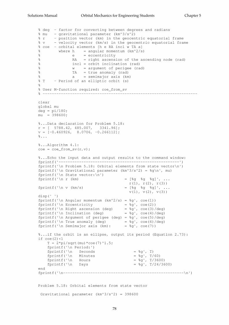
Solutions Manual Orbital Mechanics for Engineering Students Chapter 5
78
% deg - factor for converting between degrees and radians% mu - gravitational parameter (km^3/s^2)% r - position vector (km) in the geocentric equatorial frame% v - velocity vector (km/s) in the geocentric equatorial frame% coe - orbital elements [h e RA incl w TA a]% where h = angular momentum (km^2/s)% e = eccentricity% RA = right ascension of the ascending node (rad)% incl = orbit inclination (rad)% w = argument of perigee (rad)% TA = true anomaly (rad)% a = semimajor axis (km)% T - Period of an elliptic orbit (s)%% User M-function required: coe_from_sv% --------------------------------------------------------------------
clearglobal mudeg = pi/180;mu = 398600;
%...Data declaration for Problem 5.18:r = [ 5788.42, 485.007, 3341.96];v = [-0.460926, 8.0706, -0.266112];%...
%...Algorithm 4.1:coe = coe_from_sv(r,v);
%...Echo the input data and output results to the command window:fprintf('-----------------------------------------------------')fprintf('\n Problem 5.18: Orbital elements from state vector\n')fprintf('\n Gravitational parameter (km^3/s^2) = %g\n', mu)fprintf('\n State vector:\n')fprintf('\n r (km) = [%g %g %g]', ... r(1), r(2), r(3))fprintf('\n v (km/s) = [%g %g %g]', ... v(1), v(2), v(3))disp(' ')fprintf('\n Angular momentum (km^2/s) = %g', coe(1))fprintf('\n Eccentricity = %g', coe(2))fprintf('\n Right ascension (deg) = %g', coe(3)/deg)fprintf('\n Inclination (deg) = %g', coe(4)/deg)fprintf('\n Argument of perigee (deg) = %g', coe(5)/deg)fprintf('\n True anomaly (deg) = %g', coe(6)/deg)fprintf('\n Semimajor axis (km): = %g', coe(7))
%...if the orbit is an ellipse, output its period (Equation 2.73):if coe(2)<1 T = 2*pi/sqrt(mu)*coe(7)^1.5; fprintf('\n Period:') fprintf('\n Seconds = %g', T) fprintf('\n Minutes = %g', T/60) fprintf('\n Hours = %g', T/3600) fprintf('\n Days = %g', T/24/3600)endfprintf('\n-----------------------------------------------------\n')
Problem 5.18: Orbital elements from state vector
Gravitational parameter (km^3/s^2) = 398600
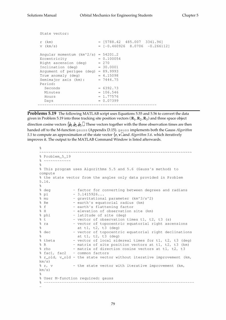
Solutions Manual Orbital Mechanics for Engineering Students Chapter 5
79
State vector:
r (km) = [5788.42 485.007 3341.96] v (km/s) = [-0.460926 8.0706 -0.266112]
Angular momentum (km^2/s) = 54201.2 Eccentricity = 0.100054 Right ascension (deg) = 270 Inclination (deg) = 30.0001 Argument of perigee (deg) = 89.9993 True anomaly (deg) = 4.15098 Semimajor axis (km): = 7444.75 Period: Seconds = 6392.73 Minutes = 106.546 Hours = 1.77576 Days = 0.07399-----------------------------------------------------
Problems 5.19 The following MATLAB script uses Equations 5.55 and 5.56 to convert the datagiven in Problem 5.19 into three tracking site position vectors ( R1, R2 , R3) and three space object
direction cosine vectors ˆ ˆ ˆρρ ρρ ρρ1 2 3, ,( ) . These vectors together with the three observation times are then
handed off to the M-function gauss (Appendix D.15). gauss implements both the Gauss Algorithm5.5 to compute an approximation of the state vector r v,( ) and Algorithm 5.6. which iterativelyimproves it. The output to the MATLAB Command Window is listed afterwards.
%~~~~~~~~~~~~~~~~~~~~~~~~~~~~~~~~~~~~~~~~~~~~~~~~~~~~~~~~~~~~~~~~~~~~% Problem_5_19% ~~~~~~~~~~~~%% This program uses Algorithms 5.5 and 5.6 (Gauss's method) tocompute% the state vector from the angles only data provided in Problem5.16.%% deg - factor for converting between degrees and radians% pi - 3.1415926...% mu - gravitational parameter (km^3/s^2)% Re - earth's equatorial radius (km)% f - earth's flattening factor% H - elevation of observation site (km)% phi - latitude of site (deg)% t - vector of observation times t1, t2, t3 (s)% ra - vector of topocentric equatorial right ascensions% at t1, t2, t3 (deg)% dec - vector of topocentric equatorial right declinations% at t1, t2, t3 (deg)% theta - vector of local sidereal times for t1, t2, t3 (deg)% R - matrix of site position vectors at t1, t2, t3 (km)% rho - matrix of direction cosine vectors at t1, t2, t3% fac1, fac2 - common factors% r_old, v_old - the state vector without iterative improvement (km,km/s)% r, v - the state vector with iterative improvement (km,km/s)%% User M-function required: gauss% --------------------------------------------------------------------
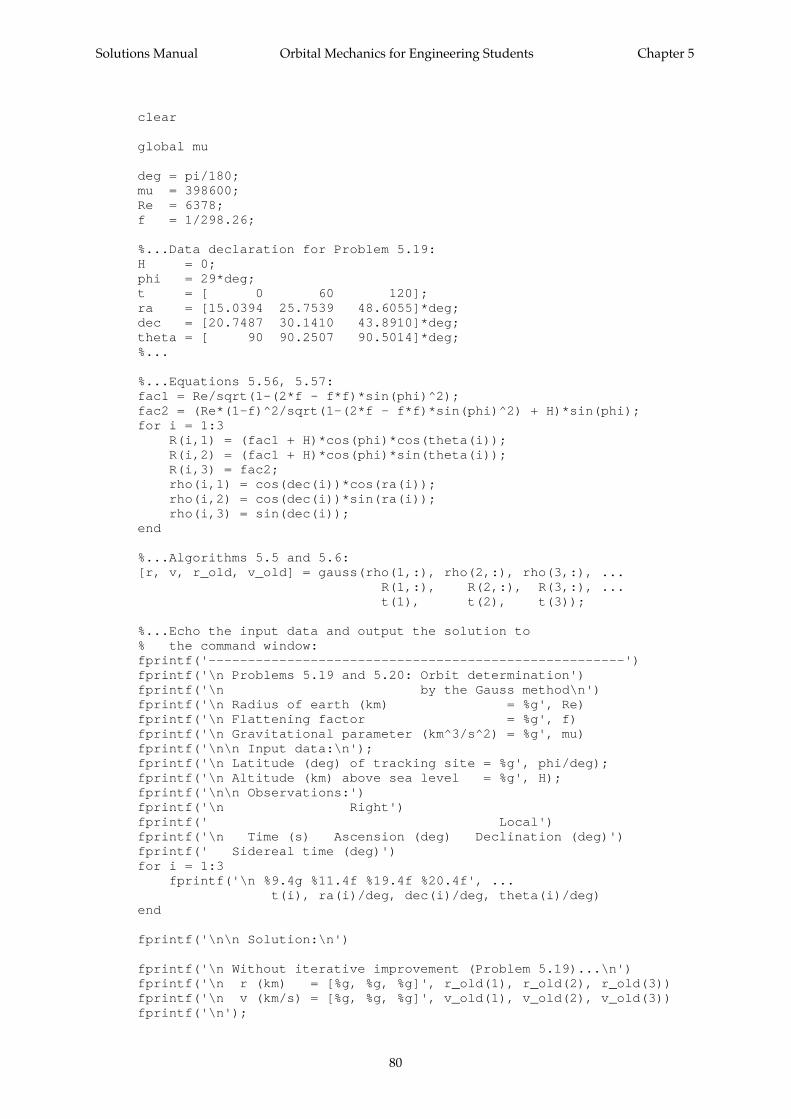
Solutions Manual Orbital Mechanics for Engineering Students Chapter 5
80
clear
global mu
deg = pi/180;mu = 398600;Re = 6378;f = 1/298.26;
%...Data declaration for Problem 5.19:H = 0;phi = 29*deg;t = [ 0 60 120];ra = [15.0394 25.7539 48.6055]*deg;dec = [20.7487 30.1410 43.8910]*deg;theta = [ 90 90.2507 90.5014]*deg;%...
%...Equations 5.56, 5.57:fac1 = Re/sqrt(1-(2*f - f*f)*sin(phi)^2);fac2 = (Re*(1-f)^2/sqrt(1-(2*f - f*f)*sin(phi)^2) + H)*sin(phi);for i = 1:3 R(i,1) = (fac1 + H)*cos(phi)*cos(theta(i)); R(i,2) = (fac1 + H)*cos(phi)*sin(theta(i)); R(i,3) = fac2; rho(i,1) = cos(dec(i))*cos(ra(i)); rho(i,2) = cos(dec(i))*sin(ra(i)); rho(i,3) = sin(dec(i));end
%...Algorithms 5.5 and 5.6:[r, v, r_old, v_old] = gauss(rho(1,:), rho(2,:), rho(3,:), ... R(1,:), R(2,:), R(3,:), ... t(1), t(2), t(3));
%...Echo the input data and output the solution to% the command window:fprintf('-----------------------------------------------------')fprintf('\n Problems 5.19 and 5.20: Orbit determination')fprintf('\n by the Gauss method\n')fprintf('\n Radius of earth (km) = %g', Re)fprintf('\n Flattening factor = %g', f)fprintf('\n Gravitational parameter (km^3/s^2) = %g', mu)fprintf('\n\n Input data:\n');fprintf('\n Latitude (deg) of tracking site = %g', phi/deg);fprintf('\n Altitude (km) above sea level = %g', H);fprintf('\n\n Observations:')fprintf('\n Right')fprintf(' Local')fprintf('\n Time (s) Ascension (deg) Declination (deg)')fprintf(' Sidereal time (deg)')for i = 1:3 fprintf('\n %9.4g %11.4f %19.4f %20.4f', ... t(i), ra(i)/deg, dec(i)/deg, theta(i)/deg)end
fprintf('\n\n Solution:\n')
fprintf('\n Without iterative improvement (Problem 5.19)...\n')fprintf('\n r (km) = [%g, %g, %g]', r_old(1), r_old(2), r_old(3))fprintf('\n v (km/s) = [%g, %g, %g]', v_old(1), v_old(2), v_old(3))fprintf('\n');
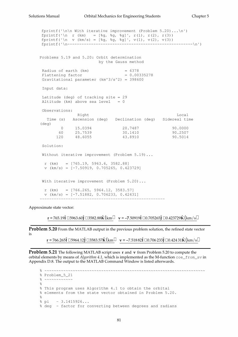
Solutions Manual Orbital Mechanics for Engineering Students Chapter 5
81
fprintf('\n\n With iterative improvement (Problem 5.20)...\n')fprintf('\n r (km) = [%g, %g, %g]', r(1), r(2), r(3))fprintf('\n v (km/s) = [%g, %g, %g]', v(1), v(2), v(3))fprintf('\n-----------------------------------------------------\n')
Problems 5.19 and 5.20: Orbit determination by the Gauss method
Radius of earth (km) = 6378 Flattening factor = 0.00335278 Gravitational parameter (km^3/s^2) = 398600
Input data:
Latitude (deg) of tracking site = 29 Altitude (km) above sea level = 0
Observations: Right Local Time (s) Ascension (deg) Declination (deg) Sidereal time(deg) 0 15.0394 20.7487 90.0000 60 25.7539 30.1410 90.2507 120 48.6055 43.8910 90.5014
Solution:
Without iterative improvement (Problem 5.19)...
r (km) = [765.19, 5963.6, 3582.88] v (km/s) = [-7.50919, 0.705265, 0.423729]
With iterative improvement (Problem 5.20)...
r (km) = [766.265, 5964.12, 3583.57] v (km/s) = [-7.51882, 0.706233, 0.42431]-----------------------------------------------------
Approximate state vector:
r I J K v= + + ( ) = −765.19 5963.60 3582.88 kmˆ ˆ ˆ 77.50919 0.705265 0.423729 km/sˆ ˆ ˆ I J K+ + ( )
Problem 5.20 From the MATLAB output in the previous problem solution, the refined state vectoris
r I J K v= + + ( ) =766.265 5964.12 3583.57 kmˆ ˆ ˆ −− + + ( )7.518 82 0.706 233 0.424 31 km/sˆ ˆ ˆ I J K
Problem 5.21 The following MATLAB script uses r and v from Problem 5.20 to compute theorbital elements by means of Algorithm 4.1, which is implemented as the M-function coe_from_sv inAppendix D.8. The output to the MATLAB Command Window is listed afterwards.
% ~~~~~~~~~~~~~~~~~~~~~~~~~~~~~~~~~~~~~~~~~~~~~~~~~~~~~~~~~~~~~~~~~~~~% Problem_5_21% ~~~~~~~~~~~~%% This program uses Algorithm 4.1 to obtain the orbital% elements from the state vector obtained in Problem 5.20.%% pi - 3.1415926...% deg - factor for converting between degrees and radians
Solutions Manual Orbital Mechanics for Engineering Students Chapter 5
82
% mu - gravitational parameter (km^3/s^2)% r - position vector (km) in the geocentric equatorial frame% v - velocity vector (km/s) in the geocentric equatorial frame% coe - orbital elements [h e RA incl w TA a]% where h = angular momentum (km^2/s)% e = eccentricity% RA = right ascension of the ascending node (rad)% incl = orbit inclination (rad)% w = argument of perigee (rad)% TA = true anomaly (rad)% a = semimajor axis (km)% T - Period of an elliptic orbit (s)%% User M-function required: coe_from_sv% --------------------------------------------------------------------
clearglobal mudeg = pi/180;mu = 398600;
%...Data declaration for Problem 5.21:r = [ 766.265, 5964.12, 3583.57];v = [-7.51882, 0.706233, 0.42431];%...
%...Algorithm 4.1:coe = coe_from_sv(r,v);
%...Echo the input data and output results to the command window:fprintf('-----------------------------------------------------')fprintf('\n Problem 5.21: Orbital elements from state vector\n')fprintf('\n Gravitational parameter (km^3/s^2) = %g\n', mu)fprintf('\n State vector:\n')fprintf('\n r (km) = [%g %g %g]', ... r(1), r(2), r(3))fprintf('\n v (km/s) = [%g %g %g]', ... v(1), v(2), v(3))disp(' ')fprintf('\n Angular momentum (km^2/s) = %g', coe(1))fprintf('\n Eccentricity = %g', coe(2))fprintf('\n Right ascension (deg) = %g', coe(3)/deg)fprintf('\n Inclination (deg) = %g', coe(4)/deg)fprintf('\n Argument of perigee (deg) = %g', coe(5)/deg)fprintf('\n True anomaly (deg) = %g', coe(6)/deg)fprintf('\n Semimajor axis (km): = %g', coe(7))
%...if the orbit is an ellipse, output its period (Equation 2.73):if coe(2)<1 T = 2*pi/sqrt(mu)*coe(7)^1.5; fprintf('\n Period:') fprintf('\n Seconds = %g', T) fprintf('\n Minutes = %g', T/60) fprintf('\n Hours = %g', T/3600) fprintf('\n Days = %g', T/24/3600)endfprintf('\n-----------------------------------------------------\n')
----------------------------------------------------- Problem 5.21: Orbital elements from state vector
Gravitational parameter (km^3/s^2) = 398600
Solutions Manual Orbital Mechanics for Engineering Students Chapter 5
83
State vector:
r (km) = [766.265 5964.12 3583.57] v (km/s) = [-7.51882 0.706233 0.42431]
Angular momentum (km^2/s) = 52946.7 Eccentricity = 0.00474691 Right ascension (deg) = 360 Inclination (deg) = 30.9997 Argument of perigee (deg) = 90.3282 True anomaly (deg) = 353.388 Semimajor axis (km): = 7033.16 Period: Seconds = 5869.98 Minutes = 97.833 Hours = 1.63055 Days = 0.0679396-----------------------------------------------------
Problem 5.22 The following MATLAB script uses the given three tracking site position vectors
( R1, R2 , R3) and three space object direction cosine vectors ˆ , ˆ , ˆρρ ρρ ρρ1 2 3( ) together with the three
observation times to find the state vector r v,( ) by means of Algorithm 5.5 and then iterativelyimprove it using Algorithm 5.6. Both algorithms are implemented in the MATLAB M-function gaussin Appendix D.15. The output to the MATLAB Command Window is listed afterwards.
% ~~~~~~~~~~~~~~~~~~~~~~~~~~~~~~~~~~~~~~~~~~~~~~~~~~~~~~~~~~~~~~~~~~~~% Problem_5_22% ~~~~~~~~~~~~%% This program uses Algorithms 5.5 and 5.6 (Gauss's method) to compute% the state vector from the angles only data provided in Problem 5.16.%% deg - factor for converting between degrees and radians% pi - 3.1415926...% mu - gravitational parameter (km^3/s^2)% t - vector of observation times t1, t2, t3 (s)% theta - vector of local sidereal times for t1, t2, t3 (deg)% R - matrix of site position vectors at t1, t2, t3 (km)% rho - matrix of direction cosine vectors at t1, t2, t3% r_old, v_old - the state vector without iterative improvement (km,km/s)% r, v - the state vector with iterative improvement (km,km/s)%% User M-function required: gauss% --------------------------------------------------------------------
clearglobal mudeg = pi/180;mu = 398600;
%...Data declaration for Problem 5.22:t = [ 0 60 120];
R = [ -1825.96 3583.66 4933.54 -1841.63 3575.63 4933.54 -1857.25 3567.54 4933.54];
rho = [-0.301687 0.200673 0.932049 -0.793090 -0.210324 0.571640
Solutions Manual Orbital Mechanics for Engineering Students Chapter 5
84
-0.873085 -0.362969 0.325539];%...
%...Algorithms 5.5 and 5.6:[r, v, r_old, v_old] = gauss(rho(1,:), rho(2,:), rho(3,:), ... R(1,:), R(2,:), R(3,:), ... t(1), t(2), t(3));
%...Echo the input data and output the solution to% the command window:fprintf('-----------------------------------------------------')fprintf('\n Problems 5.22 and 5.23: Orbit determination')fprintf('\n by the Gauss method\n')fprintf('\n Gravitational parameter (km^3/s^2) = %g', mu)fprintf('\n\n Input data:\n');fprintf('\n Site position vector (R) and space object')fprintf('\n direction cosine vector (rho) at three times:\n')for i = 1:3 fprintf('\n t = %g s:\n',t(i))
fprintf('\n R = [%g %g %g]', R(i,1), R(i,2), R(i,3))fprintf('\n rho = [%g %g %g]', rho(i,1), rho(i,2), rho(i,3))
disp(' ')endfprintf('\n\n Solution:\n')fprintf('\n Without iterative improvement (Problem 5.22)...\n')fprintf('\n r (km) = [%g, %g, %g]', r_old(1), r_old(2), r_old(3))fprintf('\n v (km/s) = [%g, %g, %g]', v_old(1), v_old(2), v_old(3))fprintf('\n');fprintf('\n\n With iterative improvement (Problem 5.23)...\n')fprintf('\n r (km) = [%g, %g, %g]', r(1), r(2), r(3))fprintf('\n v (km/s) = [%g, %g, %g]', v(1), v(2), v(3))fprintf('\n-----------------------------------------------------\n')
----------------------------------------------------- Problems 5.22 and 5.23: Orbit determination by the Gauss method
Gravitational parameter (km^3/s^2) = 398600
Input data:
Site position vector (R) and space object direction cosine vector (rho) at three times:
t = 0 s:
R = [-1825.96 3583.66 4933.54] rho = [-0.301687 0.200673 0.932049]
t = 60 s:
R = [-1841.63 3575.63 4933.54] rho = [-0.79309 -0.210324 0.57164]
t = 120 s:
R = [-1857.25 3567.54 4933.54] rho = [-0.873085 -0.362969 0.325539]
Solution:
Solutions Manual Orbital Mechanics for Engineering Students Chapter 5
85
Without iterative improvement (Problem 5.22)...
r (km) = [-2350.74, 3440.62, 5300.49] v (km/s) = [-6.61345, -3.88226, -0.413321]
With iterative improvement (Problem 5.23)...
r (km) = [-2351.59, 3440.39, 5301.1] v (km/s) = [-6.62403, -3.8885, -0.414013]-----------------------------------------------------
Approximate state vector:
r I J K v= − + + ( )2350.74 3440.62 5300.49 kmˆ ˆ ˆ == − − − ( )6.613 45 3.882 26 0.413 321 km/sˆ ˆ ˆ I J K
Problem 5.23 From the MATLAB output listed in the previous problem solution, the iterativelyimproved state vector is
r I J K v= − + + ( ) =2351.59 3440.39 5301.1 kmˆ ˆ ˆ −− − − ( )6.624 03 3.8885 0.414 013 km/sˆ ˆ ˆ I J K
Problem 5.24 The following MATLAB script uses r and v from Problem 5.23 to compute theorbital elements by means of Algorithm 4.1, which is implemented as the M-function coe_from_sv inAppendix D.8. The output to the MATLAB Command Window is listed afterwards.
%~~~~~~~~~~~~~~~~~~~~~~~~~~~~~~~~~~~~~~~~~~~~~~~~~~~~~~~~~~~~~~~~~~~~% Problem_5_24% ~~~~~~~~~~~~%% This program uses Algorithm 4.1 to obtain the orbital% elements from the state vector obtained in Problem 5.23.%% pi - 3.1415926...% deg - factor for converting between degrees and radians% mu - gravitational parameter (km^3/s^2)% r - position vector (km) in the geocentric equatorial frame% v - velocity vector (km/s) in the geocentric equatorial frame% coe - orbital elements [h e RA incl w TA a]% where h = angular momentum (km^2/s)% e = eccentricity% RA = right ascension of the ascending node (rad)% incl = orbit inclination (rad)% w = argument of perigee (rad)% TA = true anomaly (rad)% a = semimajor axis (km)% T - Period of an elliptic orbit (s)%% User M-function required: coe_from_sv% --------------------------------------------------------------------
clearglobal mudeg = pi/180;mu = 398600;
%...Data declaration for Problem 5.24:r = [-2351.59, 3440.39, 5301.1];v = [-6.62403, -3.8885, -0.414013];
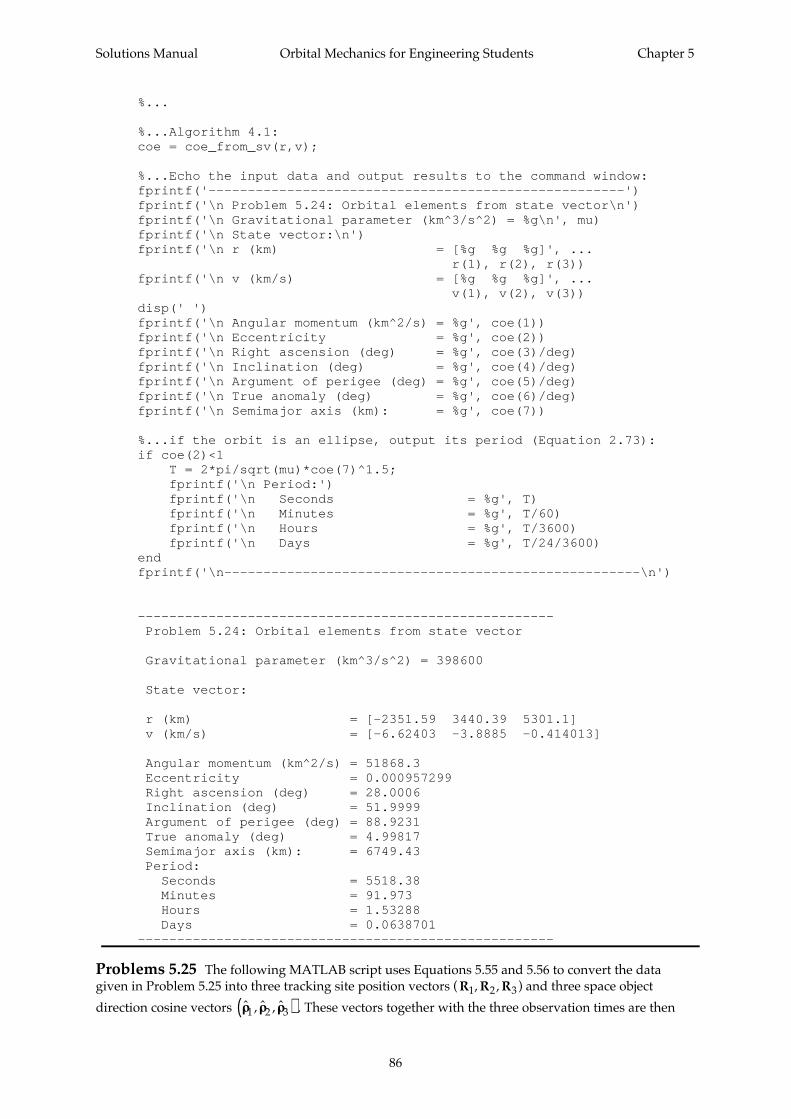
Solutions Manual Orbital Mechanics for Engineering Students Chapter 5
86
%...
%...Algorithm 4.1:coe = coe_from_sv(r,v);
%...Echo the input data and output results to the command window:fprintf('-----------------------------------------------------')fprintf('\n Problem 5.24: Orbital elements from state vector\n')fprintf('\n Gravitational parameter (km^3/s^2) = %g\n', mu)fprintf('\n State vector:\n')fprintf('\n r (km) = [%g %g %g]', ... r(1), r(2), r(3))fprintf('\n v (km/s) = [%g %g %g]', ... v(1), v(2), v(3))disp(' ')fprintf('\n Angular momentum (km^2/s) = %g', coe(1))fprintf('\n Eccentricity = %g', coe(2))fprintf('\n Right ascension (deg) = %g', coe(3)/deg)fprintf('\n Inclination (deg) = %g', coe(4)/deg)fprintf('\n Argument of perigee (deg) = %g', coe(5)/deg)fprintf('\n True anomaly (deg) = %g', coe(6)/deg)fprintf('\n Semimajor axis (km): = %g', coe(7))
%...if the orbit is an ellipse, output its period (Equation 2.73):if coe(2)<1 T = 2*pi/sqrt(mu)*coe(7)^1.5; fprintf('\n Period:') fprintf('\n Seconds = %g', T) fprintf('\n Minutes = %g', T/60) fprintf('\n Hours = %g', T/3600) fprintf('\n Days = %g', T/24/3600)endfprintf('\n-----------------------------------------------------\n')
----------------------------------------------------- Problem 5.24: Orbital elements from state vector
Gravitational parameter (km^3/s^2) = 398600
State vector:
r (km) = [-2351.59 3440.39 5301.1] v (km/s) = [-6.62403 -3.8885 -0.414013]
Angular momentum (km^2/s) = 51868.3 Eccentricity = 0.000957299 Right ascension (deg) = 28.0006 Inclination (deg) = 51.9999 Argument of perigee (deg) = 88.9231 True anomaly (deg) = 4.99817 Semimajor axis (km): = 6749.43 Period: Seconds = 5518.38 Minutes = 91.973 Hours = 1.53288 Days = 0.0638701-----------------------------------------------------
Problems 5.25 The following MATLAB script uses Equations 5.55 and 5.56 to convert the datagiven in Problem 5.25 into three tracking site position vectors ( R1, R2 , R3) and three space object
direction cosine vectors ˆ , ˆ , ˆρρ ρρ ρρ1 2 3( ) . These vectors together with the three observation times are then
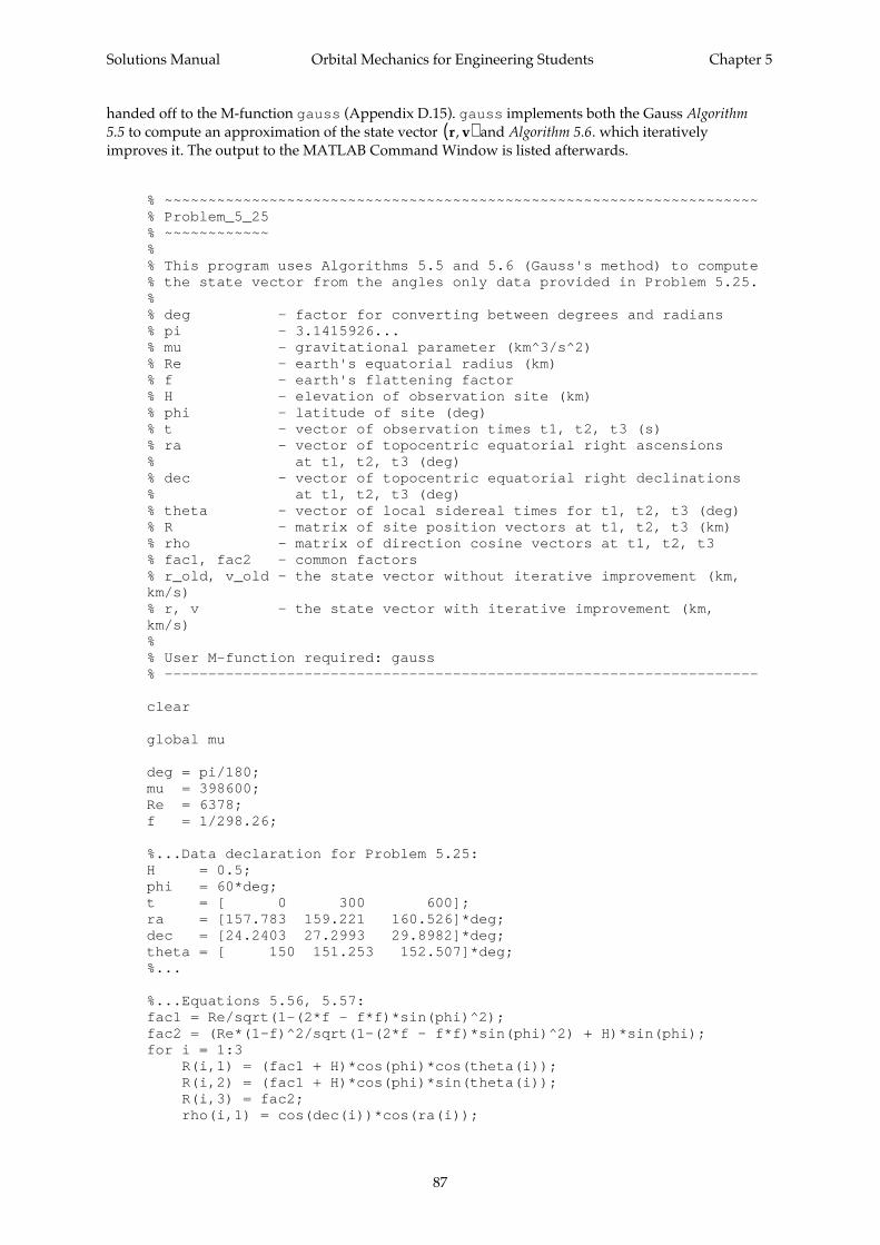
Solutions Manual Orbital Mechanics for Engineering Students Chapter 5
87
handed off to the M-function gauss (Appendix D.15). gauss implements both the Gauss Algorithm5.5 to compute an approximation of the state vector r v,( ) and Algorithm 5.6. which iterativelyimproves it. The output to the MATLAB Command Window is listed afterwards.
% ~~~~~~~~~~~~~~~~~~~~~~~~~~~~~~~~~~~~~~~~~~~~~~~~~~~~~~~~~~~~~~~~~~~~% Problem_5_25% ~~~~~~~~~~~~%% This program uses Algorithms 5.5 and 5.6 (Gauss's method) to compute% the state vector from the angles only data provided in Problem 5.25.%% deg - factor for converting between degrees and radians% pi - 3.1415926...% mu - gravitational parameter (km^3/s^2)% Re - earth's equatorial radius (km)% f - earth's flattening factor% H - elevation of observation site (km)% phi - latitude of site (deg)% t - vector of observation times t1, t2, t3 (s)% ra - vector of topocentric equatorial right ascensions% at t1, t2, t3 (deg)% dec - vector of topocentric equatorial right declinations% at t1, t2, t3 (deg)% theta - vector of local sidereal times for t1, t2, t3 (deg)% R - matrix of site position vectors at t1, t2, t3 (km)% rho - matrix of direction cosine vectors at t1, t2, t3% fac1, fac2 - common factors% r_old, v_old - the state vector without iterative improvement (km,km/s)% r, v - the state vector with iterative improvement (km,km/s)%% User M-function required: gauss% --------------------------------------------------------------------
clear
global mu
deg = pi/180;mu = 398600;Re = 6378;f = 1/298.26;
%...Data declaration for Problem 5.25:H = 0.5;phi = 60*deg;t = [ 0 300 600];ra = [157.783 159.221 160.526]*deg;dec = [24.2403 27.2993 29.8982]*deg;theta = [ 150 151.253 152.507]*deg;%...
%...Equations 5.56, 5.57:fac1 = Re/sqrt(1-(2*f - f*f)*sin(phi)^2);fac2 = (Re*(1-f)^2/sqrt(1-(2*f - f*f)*sin(phi)^2) + H)*sin(phi);for i = 1:3 R(i,1) = (fac1 + H)*cos(phi)*cos(theta(i)); R(i,2) = (fac1 + H)*cos(phi)*sin(theta(i)); R(i,3) = fac2; rho(i,1) = cos(dec(i))*cos(ra(i));
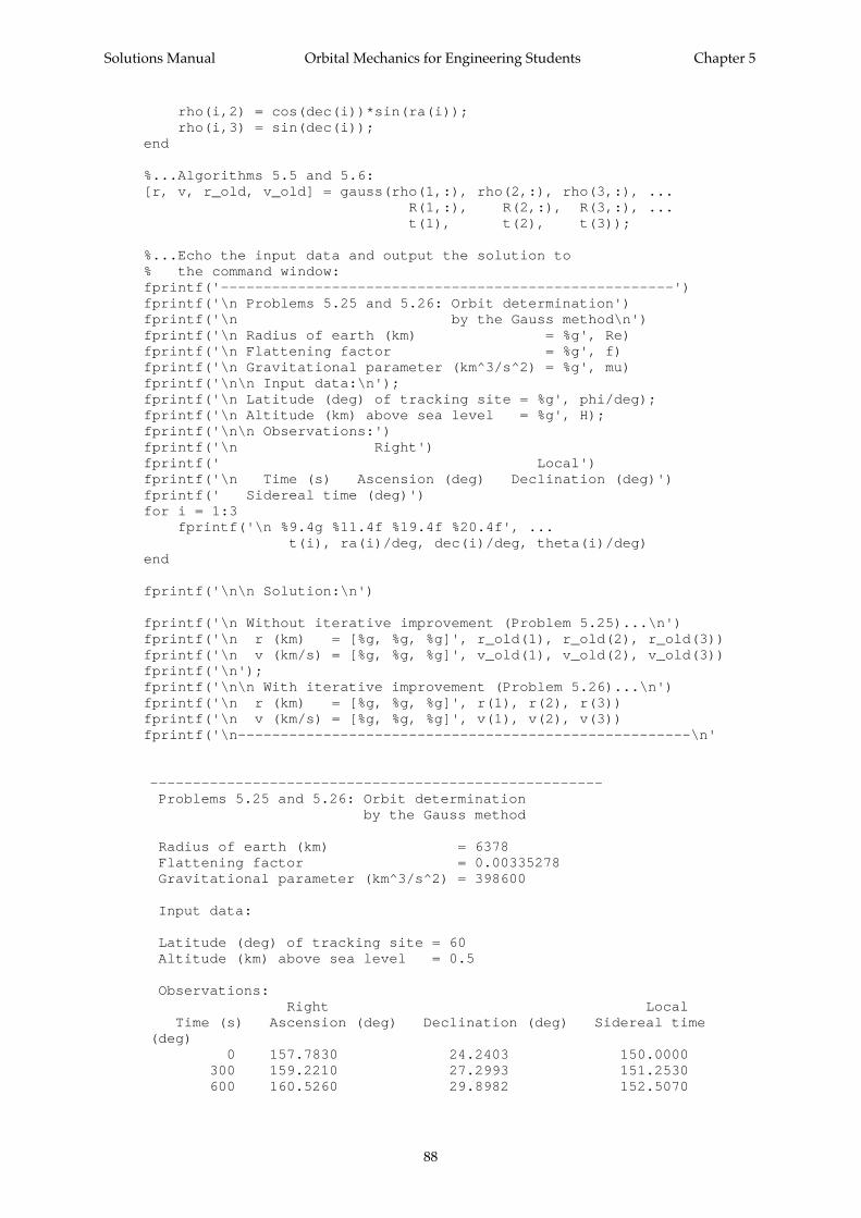
Solutions Manual Orbital Mechanics for Engineering Students Chapter 5
88
rho(i,2) = cos(dec(i))*sin(ra(i)); rho(i,3) = sin(dec(i));end
%...Algorithms 5.5 and 5.6:[r, v, r_old, v_old] = gauss(rho(1,:), rho(2,:), rho(3,:), ... R(1,:), R(2,:), R(3,:), ... t(1), t(2), t(3));
%...Echo the input data and output the solution to% the command window:fprintf('-----------------------------------------------------')fprintf('\n Problems 5.25 and 5.26: Orbit determination')fprintf('\n by the Gauss method\n')fprintf('\n Radius of earth (km) = %g', Re)fprintf('\n Flattening factor = %g', f)fprintf('\n Gravitational parameter (km^3/s^2) = %g', mu)fprintf('\n\n Input data:\n');fprintf('\n Latitude (deg) of tracking site = %g', phi/deg);fprintf('\n Altitude (km) above sea level = %g', H);fprintf('\n\n Observations:')fprintf('\n Right')fprintf(' Local')fprintf('\n Time (s) Ascension (deg) Declination (deg)')fprintf(' Sidereal time (deg)')for i = 1:3 fprintf('\n %9.4g %11.4f %19.4f %20.4f', ... t(i), ra(i)/deg, dec(i)/deg, theta(i)/deg)end
fprintf('\n\n Solution:\n')
fprintf('\n Without iterative improvement (Problem 5.25)...\n')fprintf('\n r (km) = [%g, %g, %g]', r_old(1), r_old(2), r_old(3))fprintf('\n v (km/s) = [%g, %g, %g]', v_old(1), v_old(2), v_old(3))fprintf('\n');fprintf('\n\n With iterative improvement (Problem 5.26)...\n')fprintf('\n r (km) = [%g, %g, %g]', r(1), r(2), r(3))fprintf('\n v (km/s) = [%g, %g, %g]', v(1), v(2), v(3))fprintf('\n-----------------------------------------------------\n'
----------------------------------------------------- Problems 5.25 and 5.26: Orbit determination by the Gauss method
Radius of earth (km) = 6378 Flattening factor = 0.00335278 Gravitational parameter (km^3/s^2) = 398600
Input data:
Latitude (deg) of tracking site = 60 Altitude (km) above sea level = 0.5
Observations: Right Local Time (s) Ascension (deg) Declination (deg) Sidereal time(deg) 0 157.7830 24.2403 150.0000 300 159.2210 27.2993 151.2530 600 160.5260 29.8982 152.5070
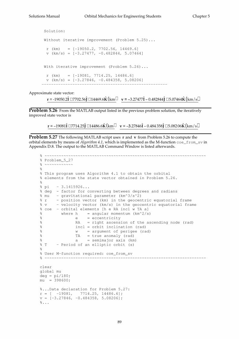
Solutions Manual Orbital Mechanics for Engineering Students Chapter 5
89
Solution:
Without iterative improvement (Problem 5.25)...
r (km) = [-19050.2, 7702.56, 14469.6] v (km/s) = [-3.27477, -0.482844, 5.07464]
With iterative improvement (Problem 5.26)...
r (km) = [-19081, 7714.25, 14486.6] v (km/s) = [-3.27846, -0.484358, 5.08206]-----------------------------------------------------
Approximate state vector:
r I J K v= + + ( )-19050.2 7702.56 14469.6 kmˆ ˆ ˆ == − − + ( )3.27477 0.482844 5.07464 km/sˆ ˆ ˆ I J K
Problem 5.26 From the MATLAB output listed in the previous problem solution, the iterativelyimproved state vector is
r I J K v= − + + ( ) = −19081 7714.25 14486.6 kmˆ ˆ ˆ 33.27846 0.484 358 5.08206 km/sˆ ˆ ˆ I J K− + ( )
Problem 5.27 The following MATLAB script uses r and v from Problem 5.26 to compute theorbital elements by means of Algorithm 4.1, which is implemented as the M-function coe_from_sv inAppendix D.8. The output to the MATLAB Command Window is listed afterwards.
% ~~~~~~~~~~~~~~~~~~~~~~~~~~~~~~~~~~~~~~~~~~~~~~~~~~~~~~~~~~~~~~~~~~~~% Problem_5_27% ~~~~~~~~~~~~%% This program uses Algorithm 4.1 to obtain the orbital% elements from the state vector obtained in Problem 5.26.%% pi - 3.1415926...% deg - factor for converting between degrees and radians% mu - gravitational parameter (km^3/s^2)% r - position vector (km) in the geocentric equatorial frame% v - velocity vector (km/s) in the geocentric equatorial frame% coe - orbital elements [h e RA incl w TA a]% where h = angular momentum (km^2/s)% e = eccentricity% RA = right ascension of the ascending node (rad)% incl = orbit inclination (rad)% w = argument of perigee (rad)% TA = true anomaly (rad)% a = semimajor axis (km)% T - Period of an elliptic orbit (s)%% User M-function required: coe_from_sv% --------------------------------------------------------------------
clearglobal mudeg = pi/180;mu = 398600;
%...Data declaration for Problem 5.27:r = [ -19081, 7714.25, 14486.6];v = [-3.27846, -0.484358, 5.08206];%...
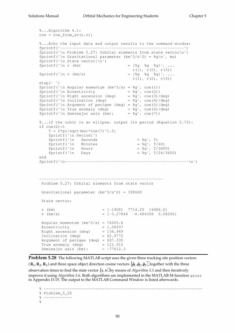
Solutions Manual Orbital Mechanics for Engineering Students Chapter 5
90
%...Algorithm 4.1:coe = coe_from_sv(r,v);
%...Echo the input data and output results to the command window:fprintf('-----------------------------------------------------')fprintf('\n Problem 5.27: Orbital elements from state vector\n')fprintf('\n Gravitational parameter (km^3/s^2) = %g\n', mu)fprintf('\n State vector:\n')fprintf('\n r (km) = [%g %g %g]', ... r(1), r(2), r(3))fprintf('\n v (km/s) = [%g %g %g]', ... v(1), v(2), v(3))disp(' ')fprintf('\n Angular momentum (km^2/s) = %g', coe(1))fprintf('\n Eccentricity = %g', coe(2))fprintf('\n Right ascension (deg) = %g', coe(3)/deg)fprintf('\n Inclination (deg) = %g', coe(4)/deg)fprintf('\n Argument of perigee (deg) = %g', coe(5)/deg)fprintf('\n True anomaly (deg) = %g', coe(6)/deg)fprintf('\n Semimajor axis (km): = %g', coe(7))
%...if the orbit is an ellipse, output its period (Equation 2.73):if coe(2)<1 T = 2*pi/sqrt(mu)*coe(7)^1.5; fprintf('\n Period:') fprintf('\n Seconds = %g', T) fprintf('\n Minutes = %g', T/60) fprintf('\n Hours = %g', T/3600) fprintf('\n Days = %g', T/24/3600)endfprintf('\n-----------------------------------------------------\n')
----------------------------------------------------- Problem 5.27: Orbital elements from state vector
Gravitational parameter (km^3/s^2) = 398600
State vector:
r (km) = [-19081 7714.25 14486.6] v (km/s) = [-3.27846 -0.484358 5.08206]
Angular momentum (km^2/s) = 76005.8 Eccentricity = 1.08937 Right ascension (deg) = 136.949 Inclination (deg) = 62.9772 Argument of perigee (deg) = 287.335 True anomaly (deg) = 112.915 Semimajor axis (km): = -77612.3
Problem 5.28 The following MATLAB script uses the given three tracking site position vectors
( R1, R2 , R3) and three space object direction cosine vectors ˆ , ˆ , ˆρρ ρρ ρρ1 2 3( ) together with the three
observation times to find the state vector r v,( ) by means of Algorithm 5.5 and then iterativelyimprove it using Algorithm 5.6. Both algorithms are implemented in the MATLAB M-function gaussin Appendix D.15. The output to the MATLAB Command Window is listed afterwards.
% ~~~~~~~~~~~~~~~~~~~~~~~~~~~~~~~~~~~~~~~~~~~~~~~~~~~~~~~~~~~~~~~~~~~~% Problem_5_28% ~~~~~~~~~~~~%
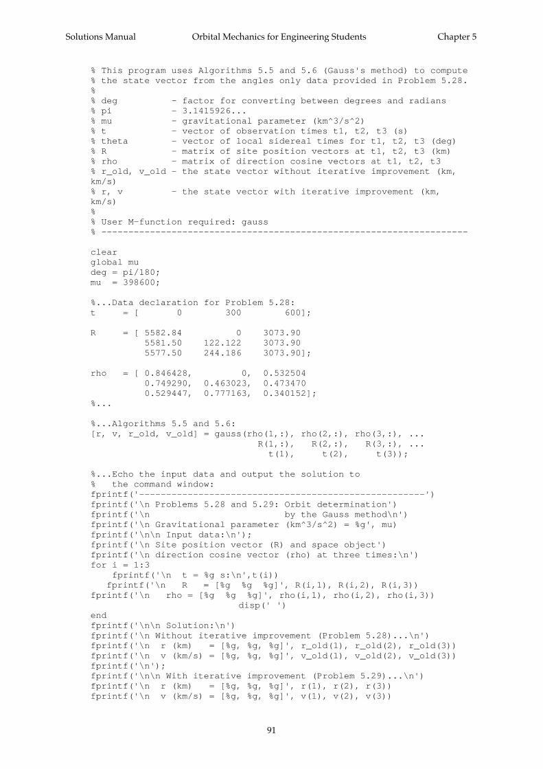
Solutions Manual Orbital Mechanics for Engineering Students Chapter 5
91
% This program uses Algorithms 5.5 and 5.6 (Gauss's method) to compute% the state vector from the angles only data provided in Problem 5.28.%% deg - factor for converting between degrees and radians% pi - 3.1415926...% mu - gravitational parameter (km^3/s^2)% t - vector of observation times t1, t2, t3 (s)% theta - vector of local sidereal times for t1, t2, t3 (deg)% R - matrix of site position vectors at t1, t2, t3 (km)% rho - matrix of direction cosine vectors at t1, t2, t3% r_old, v_old - the state vector without iterative improvement (km,km/s)% r, v - the state vector with iterative improvement (km,km/s)%% User M-function required: gauss% --------------------------------------------------------------------
clearglobal mudeg = pi/180;mu = 398600;
%...Data declaration for Problem 5.28:t = [ 0 300 600];
R = [ 5582.84 0 3073.90 5581.50 122.122 3073.90 5577.50 244.186 3073.90];
rho = [ 0.846428, 0, 0.532504 0.749290, 0.463023, 0.473470 0.529447, 0.777163, 0.340152];%...
%...Algorithms 5.5 and 5.6:[r, v, r_old, v_old] = gauss(rho(1,:), rho(2,:), rho(3,:), ... R(1,:), R(2,:), R(3,:), ... t(1), t(2), t(3));
%...Echo the input data and output the solution to% the command window:fprintf('-----------------------------------------------------')fprintf('\n Problems 5.28 and 5.29: Orbit determination')fprintf('\n by the Gauss method\n')fprintf('\n Gravitational parameter (km^3/s^2) = %g', mu)fprintf('\n\n Input data:\n');fprintf('\n Site position vector (R) and space object')fprintf('\n direction cosine vector (rho) at three times:\n')for i = 1:3 fprintf('\n t = %g s:\n',t(i))
fprintf('\n R = [%g %g %g]', R(i,1), R(i,2), R(i,3))fprintf('\n rho = [%g %g %g]', rho(i,1), rho(i,2), rho(i,3))
disp(' ')endfprintf('\n\n Solution:\n')fprintf('\n Without iterative improvement (Problem 5.28)...\n')fprintf('\n r (km) = [%g, %g, %g]', r_old(1), r_old(2), r_old(3))fprintf('\n v (km/s) = [%g, %g, %g]', v_old(1), v_old(2), v_old(3))fprintf('\n');fprintf('\n\n With iterative improvement (Problem 5.29)...\n')fprintf('\n r (km) = [%g, %g, %g]', r(1), r(2), r(3))fprintf('\n v (km/s) = [%g, %g, %g]', v(1), v(2), v(3))
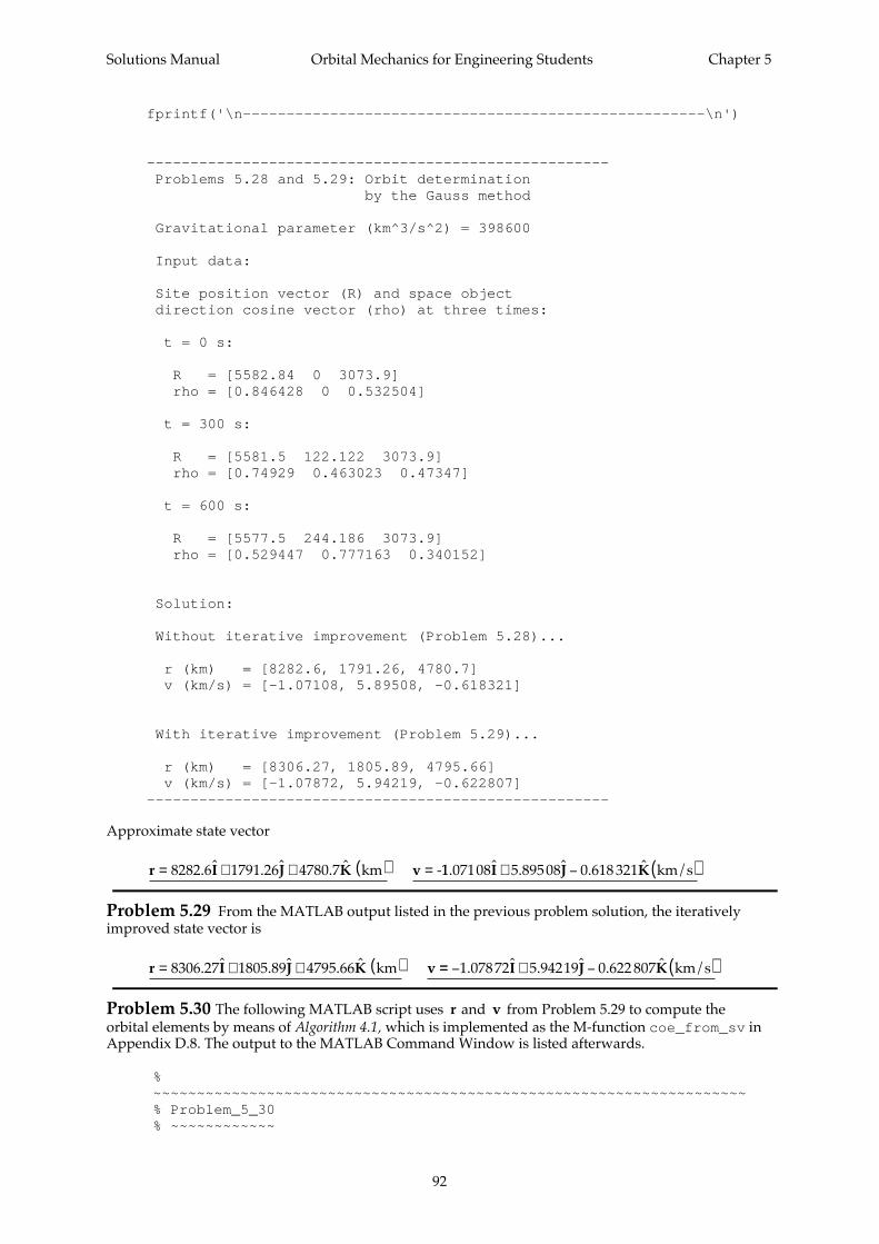
Solutions Manual Orbital Mechanics for Engineering Students Chapter 5
92
fprintf('\n-----------------------------------------------------\n')
----------------------------------------------------- Problems 5.28 and 5.29: Orbit determination by the Gauss method
Gravitational parameter (km^3/s^2) = 398600
Input data:
Site position vector (R) and space object direction cosine vector (rho) at three times:
t = 0 s:
R = [5582.84 0 3073.9] rho = [0.846428 0 0.532504]
t = 300 s:
R = [5581.5 122.122 3073.9] rho = [0.74929 0.463023 0.47347]
t = 600 s:
R = [5577.5 244.186 3073.9] rho = [0.529447 0.777163 0.340152]
Solution:
Without iterative improvement (Problem 5.28)...
r (km) = [8282.6, 1791.26, 4780.7] v (km/s) = [-1.07108, 5.89508, -0.618321]
With iterative improvement (Problem 5.29)...
r (km) = [8306.27, 1805.89, 4795.66] v (km/s) = [-1.07872, 5.94219, -0.622807]-----------------------------------------------------
Approximate state vector
r I J K v= + + ( ) =8282.6 1791.26 4780.7 km -ˆ ˆ ˆ 11.07108 5.89508 0.618 321 km/sˆ ˆ ˆI J K+ − ( )
Problem 5.29 From the MATLAB output listed in the previous problem solution, the iterativelyimproved state vector is
r I J K v= + + ( )8306.27 1805.89 4795.66 kmˆ ˆ ˆ == − + − ( )1.07872 5.94219 0.622 807 km/sˆ ˆ ˆI J K
Problem 5.30 The following MATLAB script uses r and v from Problem 5.29 to compute theorbital elements by means of Algorithm 4.1, which is implemented as the M-function coe_from_sv inAppendix D.8. The output to the MATLAB Command Window is listed afterwards.
%~~~~~~~~~~~~~~~~~~~~~~~~~~~~~~~~~~~~~~~~~~~~~~~~~~~~~~~~~~~~~~~~~~~~% Problem_5_30% ~~~~~~~~~~~~
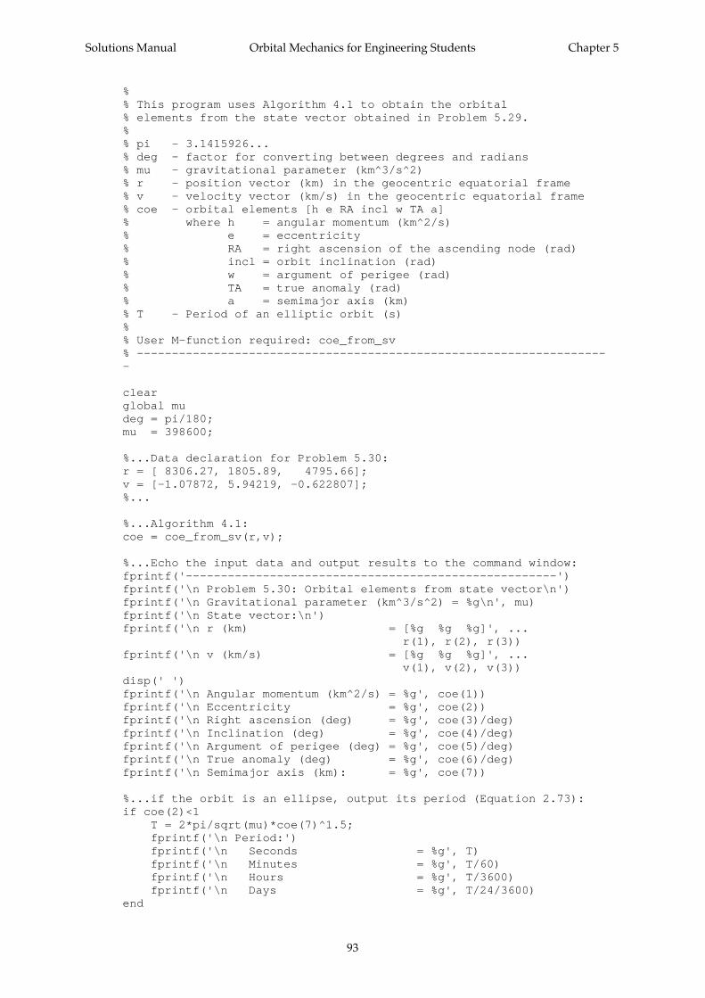
Solutions Manual Orbital Mechanics for Engineering Students Chapter 5
93
%% This program uses Algorithm 4.1 to obtain the orbital% elements from the state vector obtained in Problem 5.29.%% pi - 3.1415926...% deg - factor for converting between degrees and radians% mu - gravitational parameter (km^3/s^2)% r - position vector (km) in the geocentric equatorial frame% v - velocity vector (km/s) in the geocentric equatorial frame% coe - orbital elements [h e RA incl w TA a]% where h = angular momentum (km^2/s)% e = eccentricity% RA = right ascension of the ascending node (rad)% incl = orbit inclination (rad)% w = argument of perigee (rad)% TA = true anomaly (rad)% a = semimajor axis (km)% T - Period of an elliptic orbit (s)%% User M-function required: coe_from_sv% --------------------------------------------------------------------
clearglobal mudeg = pi/180;mu = 398600;
%...Data declaration for Problem 5.30:r = [ 8306.27, 1805.89, 4795.66];v = [-1.07872, 5.94219, -0.622807];%...
%...Algorithm 4.1:coe = coe_from_sv(r,v);
%...Echo the input data and output results to the command window:fprintf('-----------------------------------------------------')fprintf('\n Problem 5.30: Orbital elements from state vector\n')fprintf('\n Gravitational parameter (km^3/s^2) = %g\n', mu)fprintf('\n State vector:\n')fprintf('\n r (km) = [%g %g %g]', ... r(1), r(2), r(3))fprintf('\n v (km/s) = [%g %g %g]', ... v(1), v(2), v(3))disp(' ')fprintf('\n Angular momentum (km^2/s) = %g', coe(1))fprintf('\n Eccentricity = %g', coe(2))fprintf('\n Right ascension (deg) = %g', coe(3)/deg)fprintf('\n Inclination (deg) = %g', coe(4)/deg)fprintf('\n Argument of perigee (deg) = %g', coe(5)/deg)fprintf('\n True anomaly (deg) = %g', coe(6)/deg)fprintf('\n Semimajor axis (km): = %g', coe(7))
%...if the orbit is an ellipse, output its period (Equation 2.73):if coe(2)<1 T = 2*pi/sqrt(mu)*coe(7)^1.5; fprintf('\n Period:') fprintf('\n Seconds = %g', T) fprintf('\n Minutes = %g', T/60) fprintf('\n Hours = %g', T/3600) fprintf('\n Days = %g', T/24/3600)end
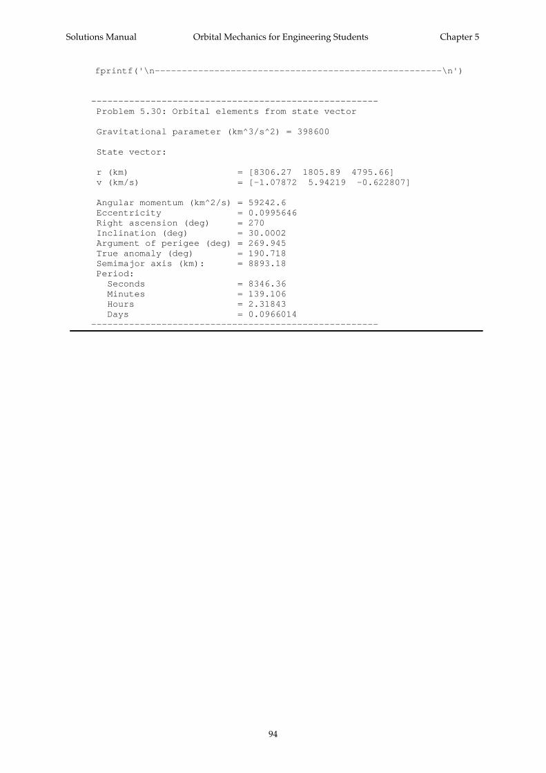
Solutions Manual Orbital Mechanics for Engineering Students Chapter 5
94
fprintf('\n-----------------------------------------------------\n')
----------------------------------------------------- Problem 5.30: Orbital elements from state vector
Gravitational parameter (km^3/s^2) = 398600
State vector:
r (km) = [8306.27 1805.89 4795.66] v (km/s) = [-1.07872 5.94219 -0.622807]
Angular momentum (km^2/s) = 59242.6 Eccentricity = 0.0995646 Right ascension (deg) = 270 Inclination (deg) = 30.0002 Argument of perigee (deg) = 269.945 True anomaly (deg) = 190.718 Semimajor axis (km): = 8893.18 Period: Seconds = 8346.36 Minutes = 139.106 Hours = 2.31843 Days = 0.0966014-----------------------------------------------------
Solutions Manual Orbital Mechanics for Engineering Students Chapter 6
95
Problem 6.1
Orbit 1 circle( ):
v
rc km /s= =+
=µ 398 600
6378 3007 726.
Orbit 2 ellipse( ):
er r
r r
rh
e
hh
vh
r
v
=−
+=
+( ) − +( )+( ) − +( ) =
=−
+ =−
⇒ =
= = =
= − =
apogee perigee
apogee perigee
apogee
2
apogeeapogee
km s
km s
km s
6378 300 6378 2006378 300 6378 200
0 003758
11
6378 300398 600
11 0 003758
51 500
51 5006678
7 711
7 726 7 711 0 01453
2
2
.
.
.
. . .
µ
∆ .
. .
..
.
. .
.
=
⋅ =
⋅ = ⋅ ⇒ =
=+ +( )
= + = + =
= = ⋅ =
=⋅
=
14 53
53 400 125000 14 53 34 01
2 27 726
14 532
7 733
7 733 34 01 263
2632 6600
0
m s
(a) s
m s
(b) km
(c) s
orbit circumference
circle circlecircle
Thrust t m v
t t
vv v v
vv
s v t
avg
avg
∆ ∆
∆ ∆
∆ ∆
∆ ∆
∆π
006006 268 0 63 or . %
Problem 6.2
v
r
r r
r
er r
r r
rh
e
hh
perigee
perigee
apogee perigee
perigee
apogee perigee
apogee perigee
apogee
2
km s
km
km
km
km s
1
1
2 1
2
22 2
2 2
22
2
2
22
2
8 2
6378 480 6858
6858
6378 160 6538
6858 65386858 6538
0 023 89
11
6858398 600
11 0 023 89
51660
=
= + =
= =
= + =
=−
+=
−+
=
=−
=−
⇒ =
.
.
.
µ
vh
r
v v v
apogeeapogee
apogee perigee
km s
km s
22
2
2 1
516606858
7 532
7 532 8 2 0 6678
= = =
= − = − = −
.
. . . ∆
Solutions Manual Orbital Mechanics for Engineering Students Chapter 6
96
Problem 6.3(a)
Orbit 1 (circle):
v
r1398 600
6378 3007 726= =
+=
µ. km s
Orbit 2 (transfer ellipse):
er r
r r
rh
e
hh
vh
r
vh
r
22 2
2 2
22
2
2
22
2
22
2
22
6378 3000 6378 3006378 3000 6378 300
0 1682
11
6678398 600
11 0 1682
55760
557606678
8 35
=−
+=
+( ) − +( )+( ) + +( ) =
=+
=+
⇒ =
= = =
=
apogee perigee
apogee perigee
perigee
2
perigeeperigee
apogeeapogee
km s
km s
.
.
.
µ
22
557609378
5 946= = . km s
Orbit 3 (circle):
v
r3398 600
6378 30006 519= =
+=
µ. km s
∆
∆
∆ ∆ ∆
v v v
v v v
v v v
1 2 1
2 3 2
1 2
8 350 7 726 0 6244
6 519 5 946 0 5734
1 198
= − = − =
= − = − =
= + =
perigee
apogee
total
km s
km s
km s
. . .
. . .
.
(b)
a r r
T a
tT
2 2 2
23 2 3 2
2
12
12
6678 9378 8028
2 2
398 6008028 7159
23579 59 65
= +( ) = +( ) =
= = = ( )
= = =
perigee apogee
perigee to apogee
km s
s period of tranfer ellipse
s m
.
/ /π
µ
π
Problem 6.4 To determine where the projectile B impacts the earth we need the orbital elements.
r
Bapogee km= 7000
v
Bapogee km s= 7 1.
h r vB B B
= = ⋅ =apogee apogee2km s7000 7 1 49700.
r
heB
B
Bapogee =
+
2 11µ
7000
49700398 600
11
0 11472
=+
⇒ =e
eB
B .
Th
eB
B
B
=−
=−
2
1
2
398 600
49700
1 0 12 2
3
2π
µ
π
. 11474952
2
3
= ( ) s period of 's orbitB
Solutions Manual Orbital Mechanics for Engineering Students Chapter 6
97
At impact, r RB = earth .
R
he
r RB
B impactBearth earthAt impact, =
+=( )
2 11µ θcos
6378
49700398 600
11 0 1147
2=
+⇒
. cos
θθ
impactimpaact = °104 3. from perigee of 's elliptical B oorbit( )
Determine the time of flight ( tof ) to impact by first finding timpact , the time from perigee to B’s
impact point.
tan tan
.
.tan
. .
E ee
Eimpact B
B
impactimpact2
11 2
1 0 11471 0 1147
104 32
1 708=−+
=−+
°⇒ =
θ rad
M E e Eimpact impact B impact= − = − =sin . . sin . .1 708 0 1147 1 708 1 594 rad
t T
Mimpact B
impact= = =
24952
1 5942
1257π π
. s (from impact point to perigee)
Then
tof
TtB
impact= − = − =2
49522
1257 1220 s
Find the orbital elements of spacecraft S trajectory.
r
Sperigee km= 7000
v vrS esc
Sperigee
perigeekm s= = =
⋅=1 3 1 3
21 3
2 398 6007000
13 97. . . . µ
h r vS S S
= = ⋅ =perigee perigee2km s7000 13 97 97 110.
r
heS
S
Sperigee =
+
2 11µ
7000
97 110398 600
11
2 382
=+
⇒ =e
eS
S .
Location of S on its hyperbolic trajectory when B impacts the earth:
M
he tofh
SS= −( ) = ⋅ −( ) ⋅ =
µ2
32 3 2 2
32 3 2
1398 600
97 1102 38 1 1220 2 131
/ /. . rad
e F F MS hsinh − =
2 38 2 131 1 118. sinh . . F F F− = ⇒ = ( )Algorihm 3.2
tan tanh
.
.tanh
. .
θθS S
SS
ee
F2
11 2
2 38 12 38 1
1 1182
76 87=+−
=+−
⇒ = °
r
heS
S
S s=
+=
+ °=
2 211
97 110398 600
11 0 28 76 87
15360µ θcos . cos .
km
distance = − =rS 6378 8978 km
Problem 6.5
(a) For the transfer ellipse
Solutions Manual Orbital Mechanics for Engineering Students Chapter 6
98
a r r= +( ) = +( ) × = ×
12
12
227 9 149 6 10 188 8 106 6Mars earth km. . .
T a= =
××( ) = ×
2 2
132 7 10188 8 10 44 73 103 2
96 3 2 6π
µ
π/ /
.. . s = 517.7 days
tof
T= =
2258 8. days time of flight from earth to Mars( )
(b) Period of Mars in its orbit,
T rMars Mars s days= =
××( ) = × =
2 2
132 7 10227 9 10 59 34 10 686 83 2
96 3 2 6π
µ
π/ /
.. . .
∴° −
°= = =
180180
2
258 8343 4
0 7537α tof
TMars
.
..
α = °44 33.
Problem 6.6
r r
e
er rr rrr
r
e
er rr rrr
r
A C
B A
B A
B
BB
D C
D C
D
DD
= =
=
=−+
=−+
⇒ =
=
=−+
=−
+⇒ =
7000 32 0000 3
0 370007000
13 000
0 5
0 532 00032 000
96 000
1
1
2
2
km km
km
km
.
.
.
.
hr r
r r
hr r
r r
hr r
r r
hr r
r
A B
A B
C D
C D
A D
A D
B C
1
2
3
4
2 2 398 6007000 13 0007000 13 000
60 230
2 2 398 60032 000 96 00032 000 96 000
138 300
2 2 398 6007000 96 0007000 96 000
72120
2
=+
= ⋅⋅
+=
=+
= ⋅⋅
+=
=+
= ⋅⋅
+=
=
µ
µ
µ
µ
km s
km s
km s
2
2
2
BB Cr+= ⋅
⋅
+=2 398 600
13 000 32 00013 000 32 000
85850 km s2
v
hr
vhrA
AA
A1
13
360 2307000
8 604721207000
10 3= = = = = =. .km s km s
v
hr
vhrB
BB
B1
14
460 23013 000
4 6338585013 000
6 604= = = = = =. .km s km s
v
hr
vhrC
CC
C2
24
4138 30032 000
4 3238585032 000
2 683= = = = = =. .km s km s
v
hr
vhrD
DD
D2
23
3138 30096 000
1 4417212096 000
0 7512= = = = = =. .km s km s

Solutions Manual Orbital Mechanics for Engineering Students Chapter 6
99
Tr r
Tr r
A D
B C
3
3 2 3 2
4
3 2 3 2
22
2
398 600
7000 96 0002
116 300 32 31
22
2
398 600
13 000 32 0002
33 590 9 33
=+
=
+
= =
=+
=
+
= =
π
µ
π
π
µ
π
/ /
/ /
.
.
s h
s h
(a) Transfer orbit 3:
∆
∆
∆ ∆ ∆
v v v
v v v
v v v
tofT
A A A
D D D
A D
= − = − =
= − = − =
= + =
= = =
3 1
2 3
33
10 3 8 604 1 699
1 441 0 7512 0 6896
2 389
232 32
216 15
. . .
. . .
.
..
km s
km s
km s
h
total
(b) Transfer orbit 4:
∆
∆
∆ ∆ ∆
v v v
v v v
v v v
tofT
B B B
C C C
B C
= − = − =
= − = − =
= + =
= = =
4 1
2 4
44
6 604 4 633 1 971
4 323 2 683 1 64
3 611
29 33
24 665
. . .
. . .
.
..
km s
km s
km s
h
total
Problem 6.7 Orbit 1 is the original circular orbit and orbit 2 is the impact trajectory.
v
rA1398 600
6378 5007 613= =
+=
µ. km s
rh
e
he
he
apogee22
2
2
22
2
22
2
11
6378 5001
16878 1
=−
+ =−
⇒ = −( )
µ
µ µ
rh
e
he
he
BB
22
2
2
22
2
22
2
11
63781
1 606378 1 0 5
=+
=+ °
⇒ = +( )
µ θ
µ µ
cos
cos .
h he e e2
22
2
2 2 26378 1 0 5 6878 1 0 04967µ µ
= ⇒ +( ) = −( ) ⇒ = . .
∴ = −( ) = ⋅ ⋅ −( ) =h e2 26878 1 6878 398 600 1 0 04967 51040µ . km s2
(a)
vhr
v v v
AA
A A
22
2 1
510406878
7 421
7 421 7 613 0 1915
= = =
= − = − = −
.
. . .
km s
km s∆
(b) To fall through the point directly below, we must remove completely the transverse component ofvelocity:
∆v vA= − = −0 7 6131 . km s
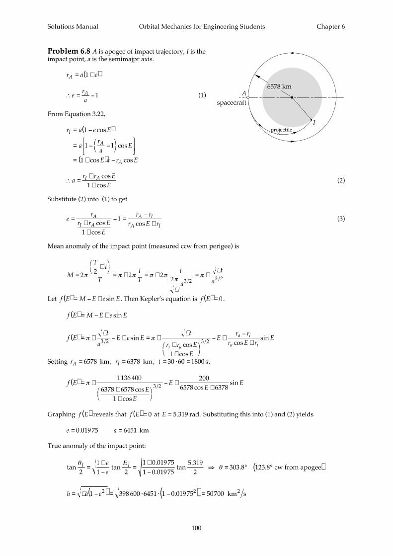
Solutions Manual Orbital Mechanics for Engineering Students Chapter 6
100
Problem 6.8 A is apogee of impact trajectory, I is theimpact point, a is the semimajpr axis.
r a eA = +( )1
∴ = −e
raA 1 (1)
From Equation 3.22,
r a e E
ara
E
E a r E
I
A
A
= −( )
= − −
= +( ) −
1
1 1
1
cos
cos
cos cos
∴ =
++
ar r E
EI A cos
cos1(2)
Substitute (2) into (1) to get
er
r r EE
r rr E r
A
I A
A I
A I=
++
− =−
+coscos
cos1
1 (3)
Mean anomaly of the impact point (measured ccw from perigee) is
M
Tt
TtT
t
a
t
a=
+
= + = + = +2 2 2 22 3 2 3 2π π π π ππ
µ
πµ
/ /
Let f E M E e E( ) = − + sin . Then Kepler’s equation is f E( ) = 0 .
f E M E e E( ) = − + sin
f Et
aE e E
t
r r EE
Er r
r E rE
i a
a i
a i( ) = + − + = +
++
− +−
+π
µπ
µ3 2 3 2
1
/ /sincos
cos
cossin
Setting r r tA I= = = ⋅ =6578 6378 30 60 1800 km km s, , ,
f EE
E
EE
E( ) = +++
− ++
π1136 400
6378 65781
2006578 63783 2cos
cos
cossin/
Graphing f E( ) reveals that f E( ) = 0 at E = 5 319. rad. Substituting this into (1) and (2) yields
e a= =0 01975 6451. km
True anomaly of the impact point:
tan tan
.
.tan
. . .
θθI Ie
e211 2
1 0 019751 0 01975
5 3192
303 8 123 8=+−
=+
−⇒ = ° °( )Ε
cw from apogee
h a e= −( ) = ⋅ ⋅ −( ) =µ 1 398 600 6451 1 0 01975 507002 2. km s2
6578 km
projectile
spacecraftA
I
Solutions Manual Orbital Mechanics for Engineering Students Chapter 6
101
v
hrAA
= = =507006578
7 707. km s velocity of projectile at apogee.
v
rc = = =µ 398 600
65787 784. km s velocity of spacecraft in circular orbit.
∆v v va c= − = − = −7 707 7 784 0 07725. . . km s
Problem 6.9
r r
r r
r
r r
apogee perigee
apogee perigee
apogee perigee
km km
km km
km km km
1 1
2 2
3
4 4
6378 302 6680 6378 296 6674
6378 291 6669 6378 259 6637
6378 259 66376378 255 6633 6378 194 6572
= + = = + =
= + = = + =
= + =
= + = = + =
.
.
hr r
r r
vh
r
vh
r
11 1
1 1
11
1
11
1
2 2 398 6006680 66746680 6674
51 590
51 5906680
7 723
51 5906674
7 730
=+
= ⋅⋅+
=
= = =
= = =
µapogee perigee
apogee perigee
2
apogeeapogee
perigeeperigee
km s
km s
km s
.
.
hr r
r r
vh
r
vh
r
22 2
2 2
22
2
21
2
2 2 398 6006669 66376669 6637
51 500
51 5006669
7 722
51 5006637
7 759
=+
= ⋅⋅+
=
= = =
= = =
µapogee perigee
apogee perigee
2
apogeeapogee
perigeeperigee
km s
km s
km s
v
r33
398 6006637
7 750= = =µ
. km s
hr r
r r
vh
r
vh
r
44 4
4 4
44
4
44
4
2 2 398 6006633 65726633 6572
51300
513006633
7 734
513006572
7 806
=+
= ⋅⋅+
=
= = =
= = =
µapogee perigee
apogee perigee
2
apogeeapogee
perigeeperigee
km s
km s
km s
.
.
Apogee of orbit 1 to perigee of orbit 2:
hr r
r r
vh
rv
hr
v
121 2
1 2
1212
11
12
22
2 2 398 6006680 66376680 6637
51 520
7 712 7 723 7 762 7 759 0 013 93
=+
= ⋅⋅+
=
= − + − = − + − =
µapogee perigee
apogee perigee
2
apogeeapogee
perigeeperigee
km s
km s∆ . . . . .
Perigee of orbit 2 to orbit 3 (tangent):
Solutions Manual Orbital Mechanics for Engineering Students Chapter 6
102
∆v v v23 2 3 7 759 7 750 0 009 313= − = − =perigee km s. . .
Orbit 3 to perigee of orbit 4:
hr r
r r
vhr
vh
rv
343 4
3 4
3434
33
34
44
2 2 398 6006572 66376572 6637
51310
7 731 7 75 7 807 7 806 0 020 26
=+
= ⋅⋅+
=
= − + − = − + − =
µperigee
perigee
2
perigeeperigee
km s
km s∆ . . . . .
∆ ∆ ∆ ∆v v v vtotal . . . . = + + = + + =12 23 34 0 013 93 0 009 313 0 020 26 0 04351 km s
Problem 6.10 r rA B= =6878 7378 km km
v
rAA
1398 600
68787 613= = =
µ. km s
h
r rr r
A B
A B2 2 2 398 600
6878 73786878 7378
53 270=+
= ⋅⋅+
=µ km s2
vhr
vhr
AA
BB
22
22
53 2706878
7 745
53 2707378
7 220
= = =
= = =
.
.
km s
km s
Alternatively, the energy equation, v r a2 2 2− = − ( )µ µ , implies
v
r a= −
2 1µ
so that, since a r rA B= +( ) =2 7128 km,
vr a
vr a
AA
BB
2
2
2 1 26878
17128
398 600 7 745
2 1 27378
17128
398 600 7 220
= −
= −
⋅ =
= −
= −
⋅ =
µ
µ
.
.
km s
km s
v
rBB
3398 600
73787 35= = =
µ. km s
∆v v v v vA A B B= − + − = + =2 1 3 2 0 1323 0 1300 0 2624. . . km s
Problem 6.11
v
rA1 =µ
h
r rr r
r2 21212
1 359=( )+
=µ µ.
v
hr rA22 1 359= = .
µ
Solutions Manual Orbital Mechanics for Engineering Students Chapter 6
103
v
hr rB2
212
0 1132= = .µ
Alternatively, using the energy equation,
ar r
r
vr a r r
vr a r r
A
B
2
22
22
122
6 5
2 11 846 1 359
212
10 01282 0 1132
=+
=
= −
= =
= −
= =
.
. .
. .
µµ µ
µµ µ
v
r rB3 120 2887= =
µ µ.
∆v v v v v
r r rA A B B= − + − = + =2 1 3 2 0 3587 0 1754 0 5342. . .µ µ µ
Problem 6.12
v
rv
r rA A1 22
1 414= = =µ µ µ
.
v
r rv
r rB B3 4212
0 408212
0 2887= = = =µ µ µ µ
. .
∆v v v v v
r r rA A B B= − + − = + =2 1 4 3 0 4142 0 1196 0 5338. . .µ µ µ
Problem 6.13 r r r rA B= = 3
v v
r rAA
1 1= = =µ µ
hr r
r rr rr r
r
vhr
rr r
vhr
rr r
A B
A B
AA
BB
2
22
22
2 233
1 225
1 2251 225
1 2253
0 4082
=+
=( )+
=
= = =
= = =
µ µ µ
µ µ
µ µ
.
..
..
(Alternatively, use the energy equation.)
v vr r r
v v v v vr r r
v
BB
A A B B
3 3
2 1 3 2 1
30 5774
0 2247 0 1691 0 3938 0 3938
= = = =
= − + − = + = =
µ µ µ
µ µ µ
.
. . . .∆
Problem 6.14 r rA C= =6678 9378 km km (a)Orbit 1:
v
rAA
1398 600
66787 726= = =
µ. km s
Orbit 2:
Solutions Manual Orbital Mechanics for Engineering Students Chapter 6
104
r rr r
e
rr
r
B A
B A
B
BB
−+
=
−+
= ⇒ =
2
66786678
0 3 12 402. km
hr r
r r
vhr
vhr
A B
A B
AA
BB
2
22
22
2 2 398 6006678 12 4026678 12 402
58 830
58 8306678
8 809
58 83012 402
4 743
=+
= ⋅⋅
+=
= = =
= = =
µ km s
km s
km s
2
.
.
Orbit 3:
hr r
r r
vhr
vhr
B C
B C
BB
CC
3
33
33
2 2 398 60012 402 937812 402 9378
65250
6525012 402
5 261
652509378
6 957
=+
= ⋅⋅
+=
= = =
= = =
µ km s
km s
km s
2
.
.
Orbit 4:
v
rCC
4398 6009 378
6 519= = =µ
. km s
∆v v v v v v vtotal A A B B C C= − + − + − = + + =2 1 3 2 4 3 1 083 0 5177 0 4379 2 039. . . . km s
(b)
Tr r
Tr r
t T T
A B
B C
total
2
3 2 3 2
3
3 2 3 2
1 2
22
2
398 600
6678 12 4022
9273
22
2
398 600
12 402 93782
11310
12
10 290 2 859
=+
=
+
=
=+
=
+
=
= +( ) = =
π
µ
π
π
µ
π
/ /
/ /
.
s
s
s hr
Problem 6.15 r r r r rA C E B D= = = = =15000 22 000 6878 km km km(a)Orbit 1:
vrAA
A
) = = =
=
1
1
398 60015000
5 155µ
γ
. km s
Orbit 2:
er rr r
hr r
r r
B D
B D
B D
B D
2
2
22 000 687822 000 6878
0 5237
2 2 398 60022 000 687822 000 6878
64 630
=−+
=−
+=
=+
= ⋅⋅
+=
.
µ km s2
At the maneuvering point A:

Solutions Manual Orbital Mechanics for Engineering Students Chapter 6
105
rh
eAA
AA
=+
=+
⇒ = °
22
22
11
1500064 630398 600
11 0 5237
125 1
µ θ
θθ
cos
. cos .
v
hrAA
22 64 630
150004 309) = = =
⊥. km s
v
heA r A2
22
398 60064 630
0 5237 125 1 2 641) = = ° =µ
θsin . sin . . km s
v v vA A A r2 2
22
2 2 24 309 2 641 5 054= ) + ) = + =⊥
. . . km s
γ γAA r
AA
v
v21 2
2
12
2 6414 309
0 5499 31 51=))
= = ⇒ = °−
⊥
−tan tan..
. .
∆γ γ γA A A= − = ° − = °2 1 31 51 0 31 51. .
∆ ∆ ∆v v v v vA A A A A A A= + − = + − =1
22
21 2
2 22 5 155 5 054 25 1555 054 2 773cos . . . . cos .γ γ km s T
(b)Try Hohmann transfer (orbit 3) from point E on orbit 1 to point B on orbit 2.
h
r rr r
E B
E B3 2 2 398 600
15000 22 00015000 22 000
84 320=+
= ⋅⋅
+=µ km s2
v v
vhr
vhr
vhr
v v v v v
E A
EE
BB
BB
total E E B B
1
1
1
33
33
22
3 2 3
5 155
84 32015000
5 621
84 32022 000
3 833
64 63022 000
2 938
0 4665 0 985 1 362
= =
= = =
= = =
= = =
= − + − = + =
.
.
.
.
. . .
km s
km s
km s
km s
km s∆
Try Hohmann transfer (orbit 4) from point C on orbit 1 to point D on orbit 2.
h
r rr r
C D
C D4 2 2 398 600
15000 687815000 6878
61310=+
= ⋅⋅
+=µ km s2
v v
vhr
vhr
vhr
v v v v v
C A
CC
DD
DD
total C C D D
1 1
44
44
42
4 2 4
5 155
6131015000
4 088
613106878
8 914
64 6306878
9 397
1 067 0 4824 1 551
= =
= = =
= = =
= = =
= − + − = + =
.
.
.
.
. . .
km s
km s
km s
km s
km s∆
This is larger than the total computed above; thus for minimum Hohmann transfer
∆v = 1 362. km s
Solutions Manual Orbital Mechanics for Engineering Students Chapter 6
106
Problem 6.16
Orbit 1:
r
v
h r v
rh
e
ee
perigee
perigee
perigee perigee2
perigee
km
km s
km s
1
1
1 1 1
11
2
12
11
6378 1270 7648
9
7648 9 68 832
11
764868 832398 600
11
0 5542
= + =
=
= = ⋅ =
=+
=+
⇒ =
.
µ
At the maneuver point, θ = °100 .
r
he
=+
=+ °
=12
1
211
68 832398 600
11 0 5542 100
13150µ θcos . cos
km
vhr
vh
e
v v v
v
v
r
r
r
11
11
1
1 12
12 2 2
11 1
1
1
68 83213150
5 234
398 60068 832
0 5542 100 3 16
5 234 3 16 6 114
3 165 234
31 13
⊥
⊥
−
⊥
−
= = =
= = ° =
= + = + =
= = =
.
sin . sin .
. . .
tan tan..
.
km s
km s
km s
µθ
γ
Orbit 2:
e
rh
e
hh
2
22
2
22
2
0 4
11
13150398 600
11 0 4 100
69 840
=
=+
=+ °
⇒ =
.
cos
. cos
µ θ
km s2
vhr
vh
e
v v v
v
v
r
r
r
22
22
2
2 22
22 2 2
21 2
2
1
69 84013150
5 311
398 60069 840
0 4 100 2 248
5 311 2 248 5 767
2 2485 767
22 94
⊥
⊥
−
⊥
−
= = =
= = ° =
= + = + =
= = = °
.
sin . sin .
. . .
tan tan..
.
km s
km s
km s
µθ
γ
∆
∆ ∆
γ γ γ
γ
= − = ° − ° = − °
= + − = + − ⋅ ⋅ −( ) =
2 1
12
22
1 22 2
22 94 31 13 8 181
2 6 114 5 767 2 6 114 5 767 8 181 0 9155
. . .
cos . . . . cos . . v v v v v km s
Problem 6.17 r vA A A= = = °12756 6 5992 20 km km . γ
Orbit 1:
v v
h r v
A A A
A A
⊥
⊥
= = ° =
∴ = = ⋅ =
cos . cos .
. .
γ 6 5992 20 6 20122
12756 6 20122 79102 81
km s
km s2

Solutions Manual Orbital Mechanics for Engineering Students Chapter 6
107
v v
vh
e
e e
Ar A A
Ar A
A A
= = ⋅ ° =
=
= ⇒ =
sin . sin .
sin
..
sin sin .
γ
µθ
θ θ
6 5992 20 2 25706
2 25706398 60079102 8
0 447 917
11
1 1
km s
rh
e
ee
AA
AA
=+
=+
⇒ =
12
12
11
11
1275679102 8398 600
11
0 230 641
µ θ
θθ
cos
.cos
cos .
∴ +( ) = +e A A12 2 2 2 20 447 917 0 230 641sin cos . .θ θ
e e12
10 253 825 0 503 81= ⇒ =. .
∴ = = ⇒ = ° = °sin
..
. . .θ θ θA A A0 447 9170 503 81
0 889 058 62 7552 117 235 or
Since cosθA > 0 , θA = °62 7552. .
rh
e
vhr
vh
e
BB
BB
Br B
=+
=+ °
=
) = = =
) = = ⋅ ⋅ ° =
⊥
12
1 1
2
11
1 11 1
11
79102 8398 600
11 0 503 81 150
27 848 9
79102 827 848 9
2 840 43
398 60079102 8
0 503 81 150 1 269 45
µ θ
µθ
cos.
. cos.
..
.
sin.
. sin .
km
km s
km s
Orbit 2:
∆
∆
v
v v vB
B B B
⊥
⊥ ⊥ ⊥
=
∴ ) = ) + = + =
0 758 20
2 840 43 0 758 20 3 598 632 1
.
. . .
km s
km s
h r vB B2 2
27 848 9 3 598 63 100 218= ) = ⋅ =⊥ . . km s2
∆
∆
v
v v vBr
Br Br B
=
∴ ) = ) + = + =⊥
0
1 269 45 0 1 269 452 1
. . km s
vh
e
e e
Br B
B B
) =
= ⇒ =
2 22 2
2 2 2 21 269 45398 600100 218
0 319146
µθ
θ θ
sin
. sin sin .
rh
e
ee
BB
BB
=+
=+
⇒ = −
22
2 22
2 22 2
11
27 848 9100 218398 600
11
0 095216 6
µ θ
θθ
cos
.cos
cos .
AB
150°
1
2
Solutions Manual Orbital Mechanics for Engineering Students Chapter 6
108
e
e
e
B B22 2
22
22 2
22
2
0 319146 0 095216 6
0 110 9210 333 048
sin cos . .
.
.
θ θ+( ) = + −( )=
=
∴ = = ⇒ = ° °sin
.
.. . θ θB B2 2
0 3191460 333 048
0 958 261 73 387 7 or 106.612
Since cosθB2 0< , θB2 = °106.612 .
∆θ = − ° = °150 43 3877106.612 .
That is, the apse line is rotated 43.387 7° ccw from that of orbit 1.
Problem 6.18
r r
he
he
1 22 21
11
1
22
=
+=
+ −( )= −( )
∴ = − ⇒ = ⇒ =
µ θ µ η θ
θ η θ
θ η θ θ η θη
cos cos
cos cos
Problem 6.19
Orbit 1:
r
heP1
12 1
1=
+µ
Orbit 2:
r
he
hP1
22
221
1 90=
+ °=
µ µcos
∴ =
+⇒ =
+
h he
hh
e2
21
2
211
1 1µ µ
Problem 6.20
At A:
r
h=
2
µ
v
he
her1 90= ° =
µ µsin
v
he
her2 90= − °( ) = −
µ µsin
v v
hr⊥ ⊥= =1 2
∴ =⊥∆v 0
∆v v v
her r r= − = −2 1 2
µ
Solutions Manual Orbital Mechanics for Engineering Students Chapter 6
109
∴ = =∆ ∆v v
ehr
2µ
Problem 6.21 For the circular orbit of the space station,
r v
rT rc c= = = = = = =6728
398 6006728
7 6972 2
398 6006728 54923 2 3 2 km km s s = 91.54 m . / /µ π
µ
π
(a) The time required for spacecraft A to reach the space station is the time it takes for the spacestation to fly around to the original position of spacecraft A.
t T
rrSA c = s = 90.2 min
2 6002
54922 6728 600
2 67285414
ππ
π
π−
=⋅ −
⋅=
The time required for spacecraft B to reach the space station is the time it takes for the space station tofly around to the original position of spacecraft B.
t T
rrBS c = s = 92.8 min
2 6002
54922 6728 600
2 67285570
ππ
π
π+
=⋅ +
⋅=
(b)
The period of spacecraft A’s phasing orbit, is tSA, which determines the semimajor axis of that orbit:
5414
2
398 60066643 2= ⇒ =
πa aA A
/ km
Spacecraft A is at the apogee of its phasing orbit. From the energy equation
v
r aAA
= −
= −
=µ
2 1398 600
26728
16664
7 660. km s
The delta-v required to drop into the phasing orbit is
∆v v vA A c= − = − = −7 660 7 697 0 036 94. . . km s
Spacecraft A must therefore slow down in order to speed up (i.e., catch the space station). After onecircuit of its phasing orbit, this delta-v must be added in order to rejoin the circular orbit. Thus
∆ ∆v vAtotal A= =2 0 073 88. km s
The period of spacecraft B’s phasing orbit, is tBS, which determines the semimajor axis of thatorbit:
5570
2
398 60067913 2= ⇒ =
πa aB B
/ km
Spacecraft B is at the perigee of its phasing orbit. From the energy equation
v
r aBB
= −
= −
=µ
2 1398 600
26728
16791
7 733. km s
The prograde delta-v required to enter the phasing orbit is
Solutions Manual Orbital Mechanics for Engineering Students Chapter 6
110
∆v v vB B c= − = − = +7 733 7 697 0 03576. . . km s
Spacecraft B must therefore speed up in order to slow down (i.e, allow the space station to catch up).After one circuit of its phasing orbit, this delta-v must be subtracted in order to rejoin the circularorbit. Thus
∆ ∆v vBtotal B= =2 0 071 53. km s
Problem 6.22
TT
a r
a r
a r a r
phasing =
=
=
=
⇒ =
22 1
22
12
12
0 63
3 2 3 2
3 2 3 2
3 22 3
π
µ
π
µ/ /
/ /
//
.
Problem 6.23 r rA P= =13 000 8000 km km
Orbit 1:
ar r
er rr r
h e r
T a
A P
A P
A P
P
1
1
1
13 2 3 2
210 500
0 2381
1 398 600 1 0 2381 8000 62 830
2 2
398 60010 500 10710
=+
=
=−+
=
= +( ) = +( ) ⋅ =
= = =
.
.
/ /
km
km s
s
2µ
π
µ
π
Time of flight from P to C:
Eee
M E e E
tM
T
CC
C C C
CC
=−+
=
−+
°
=
= − = − =
= = ⋅ =
− −tan tan tan..
tan .
sin . . sin . ..
.
1 1
1
1
1
11 2
1 0 23811 0 2381
302
0 4144
0 4144 0 2381 0 4144 0 3185
20 3185
210710 542 8
θ
π π
rad
rad
s
Time of flight from P to D:
Eee
M E e E
tM
T
DD
D D d
DD
=−+
=
−+
°
=
= − = − =
= = ⋅ =
− −tan tan tan..
tan .
sin . . sin . ..
1 1
1
1
1
11 2
1 0 23811 0 2381
902
1 330
1 330 0 2381 1 330 1 099
21 099
210710 1873
θ
π π
rad
rad
s
Time of flight from C to D:
t t tCD D C= − = − =1873 542 8 1330. s
To determine the trajectory from P to D is Lambert’s problem. Note that
r
heD
D=
+=
+ °=1
2
1
211
62 830398 600
11 0 2381 90
9905µ θcos . cos
km

Solutions Manual Orbital Mechanics for Engineering Students Chapter 6
111
so that in perifocal coordinates
r p r qP D= =8000 9905ˆ ˆ km km
Note as well, that on orbit 1,
v p qP P Phe1
1
398 60062 830
= − + +( ) =µ
θ θsin ˆ cos ˆ −− + +( )
= ( )
sin ˆ . cos ˆ
. ˆ
0 0 2381 0
7 854
p q
q
v
km s
D111
398 60062 830
= − + +( ) = −µ
θ θh
eD Dsin ˆ cos ˆp q ssin ˆ . cos ˆ
. ˆ .
90 0 2381 90
6 344 1
° + + °( )
= − +
p q
p 5510q km s( )
The following MATLAB script calls upon Algorithm 5.2, implemented as the M-function lambert inAppendix D.11, to solve Lamberts’ problem for the velocities on orbit 2 at P and D. The output to theMATLAB Command Window is listed afterwards.
%~~~~~~~~~~~~~~~~~~~~~~~~~~~~~~~~~~~~~~~~~~~~~~~~~~~~~~~~~~~~~~~~~~~~% Problem 6_23% ~~~~~~~~~~~~%% This program uses Algorithm 5.2 to solve Lambert's problem for the% data of in Problem 6.23.
% deg - factor for converting between degrees and radians% pi - 3.1415926...% mu - gravitational parameter (km^3/s^2)% r1, r2 - initial and final radii (km)% dt - time between r1 and r2 (s)% dtheta - change in true anomaly during dt (degrees)% R1, R2 - initial and final position vectors (km)% string - = 'pro' if the orbit is prograde% = 'retro if the orbit is retrograde% V1, V2 - initial and final velocity vectors (km/s)
% User M-function required: lambert% -----------------------------------------------------------clearglobal mumu = 398600; %km^3/s^2deg = pi/180;
r1 = 8000; %kmr2 = 9905; %kmdt = 1330; %secdtheta = 90; %degrees
R1 = [r1 0 0];R2 = [r2*cos(dtheta*deg) r2*sin(dtheta*deg) 0];
%...Algorithm 5.2:string = 'pro';[V1 V2] = lambert(R1, R2, dt, string);
%...Echo the input data and output results to the command window:fprintf('\n-----------------------------------------------------')fprintf('\n Problem 6.23: Lambert''s Problem\n')
fprintf('\n Input data:\n');
Solutions Manual Orbital Mechanics for Engineering Students Chapter 6
112
fprintf('\n Gravitational parameter (km^3/s^2) = %g\n', mu)fprintf('\n Radius 1 (km) = %g', r1)fprintf('\n Position vector R1 (km) = [%g %g %g]\n',... R1(1), R1(2), R1(3))fprintf('\n Radius 2 (km) = %g', r2)fprintf('\n Position vector R2 (km) = [%g %g %g]\n',... R2(1), R2(2), R2(3))fprintf('\n Elapsed time (s) = %g', dt)fprintf('\n Change in true anomaly (deg) = %g', dtheta)
fprintf('\n\n Solution:\n')fprintf('\n Velocity vector V1 (km/s) = [%g %g %g]',... V1(1), V1(2), V1(3))fprintf('\n Velocity vector V2 (km/s) = [%g %g %g]',... V2(1), V2(2), V2(3))fprintf('\n-----------------------------------------------------\n')
----------------------------------------------------- Problem 6.23: Lambert's Problem
Input data:
Gravitational parameter (km^3/s^2) = 398600
Radius 1 (km) = 8000 Position vector R1 (km) = [8000 0 0]
Radius 2 (km) = 9905 Position vector R2 (km) = [-0 9905 0]
Elapsed time (s) = 1330 Change in true anomaly (deg) = 90
Solution:
Velocity vector V1 (km/s) = [-2.53168 9.57638 0] Velocity vector V2 (km/s) = [-7.73458 4.37347 0]-----------------------------------------------------
v p q
v pP
D
2
2
2 532 9 576
7 734 4 37
= − + ( )= − +
. ˆ . ˆ
. ˆ .
km s
33 ˆ q km s( )
∆v v v p q qP P P= − = − +( ) − = −2 1 2 532 9 576 7 854 2 5. ˆ . ˆ . ˆ . 332 1 722
2 532 1 722 3 02 2
ˆ . ˆ
. . .
p q
v
+ ( )
= −( ) + =
km s
∆ P 662 km s( )
∆v v v p q pD D D= − = − +( ) − − +2 1 7 734 4 373 6 344 1 5. ˆ . ˆ . ˆ . 110 1 391 2 863
1 391 2
ˆ . ˆ . ˆ
.
q p q
v
( ) = − + ( )
= −( )
km s
∆ D ++ = ( )2 863 3 1832. . km s
∆ ∆ ∆vtotal P D= + = + =v v 3 062 3 183 6 245. . . km s
Problem 6.24
h a e= −( ) = ⋅ ⋅ −( ) =µ 1 398 600 15000 1 0 5 66 9602 2. km s2
r
heascending node km=
+ −( ) =+ − °( ) =
2 211
66 960398 600
11 0 5 30
7851µ ωcos . cos
Solutions Manual Orbital Mechanics for Engineering Students Chapter 6
113
r
hedescending node km=
+ − +( ) =+ − ° + °( ) =
2 211
66 960398 600
11 0 5 30 180
19 840µ ω πcos . cos
Rotate the orbital plane 10 degrees around the node line. That means hold vr fixed and rotate v⊥ 10degrees. For minimum delta-v, do this maneuver at the furthest distance from the focus (at thedescending node, rather than the ascending node).
vh
r
v vi
⊥
⊥
= = =
= = ⋅ ⋅°
=
descending nodekm s
km s
66 96019 840
3 375
22
2 3 375102
0 5883
.
sin . sin . ∆∆
(Note: if the maneuver is done at the ascending node,
vh
r
v vi
⊥
⊥
= = =
= = ⋅ ⋅°
=
ascending nodekm s
km s
66 9607851
8 53
22
2 8 53102
1 487
.
sin . sin .∆∆
Over twice the delta-v requirement.)
Problem 6.25 For the circular orbit
v
r1398 600
67787 668= = =
µ. km s
Assume the maneuver is done at apogee of the ellipse (orbit 2).
rh
e
hh
=−
=−
⇒ =
22
2
22
2
11
6778398 600
11 0 5
36750
µ
. km s2
Then
r
heperigee km=
+=
+=2
2
2
211
36750398 600
11 0 5
2259µ .
which is inside the earth. So the maneuver cannot occur at apogee. Assume it occurs at perigee.
rh
e
hh
=+
=+
⇒ =
22
2
22
2
11
6778398 600
11 0 5
63 660
µ
. km s2
v
hr22 63 660
67789 392= = = . km s
∆v v v v v= + − = + − ⋅ ⋅ =1
22
21 2
2 22 7 668 9 392 2 7 668 9 392 3 414cos . . . . cos . δ δ km s
Solutions Manual Orbital Mechanics for Engineering Students Chapter 6
114
Problem 6.26
rh
e
vh
r
v v
apogee
apogeeapogee
apogee
km
km s
km s
=−
=−
=
= = =
= = ⋅°
=
2 211
60 000398 600
11 0 3
12 900
60 00012 900
4 65
22
2 4 65902
6 577
µ
δ
.
.
sin . sin . ∆
Problem 6.27
vr
rh
eh h
h r
Bo
o o
1
22
22
22
21
11
1 0 25 90
=
=+
=+ − °( ) = ⇒ =
µ
µ θ µ µµ
cos . cos
vhr
r
r r
vh
er r
Bo
o
o o
Bro o
⊥ = = =
= = ⋅ ⋅ − °( ) = −
22
2 22 0 25 90 0 25
µ µ
µθ
µ
µ
µsin . sin .
∆v v v v v v vBr Br B B B B= −( ) + + −⊥ ⊥ ⊥ ⊥2 1
212
22
1 22 cosδ
∆v
r r r r ro o o o o= − −
+ + − − °( )0 25 0 2 90
2 2 2
. cosµ µ µ µ µ
∆
∆
∆
vr r r
vr
vr
o o o
o
o
= + + −
=
=
0 0625 0
2 0625
1 436
.
.
.
µ µ µ
µ
µ
Problem 6.28 The initial and target orbits are “1” and “2”, respectively, and “3” is the transferorbit.
r1 6678= km
v
r11
398 6006678
7 726= = =µ
. km s
r2 6978= km
v
r22
398 6006978
7 558= = =µ
. km s
a
r r3
1 22
6678 69782
6828=+
=+
= km
v
r aperigee km s3 1 3
2 1398 600
26678
16828
7 810= −
= −
=µ .
v
r aapogee km s3 2 3
2 1398 600
26978
16828
7 474= −
= −
=µ .
Solutions Manual Orbital Mechanics for Engineering Students Chapter 6
115
(a)
∆∆
v v v v v vi
= −( ) + −( ) + ⋅
= −( ) + −( ) + ⋅°
= + + =
perigee apogee
km s
3 1 2 3 222
7 810 7 726 7 558 7 474 2 7 558202
0 0844 0 083 48 2 625 2 793
sin
. . . . . sin
. . . . (b)
∆ ∆v v v v v v v i= −( ) + + −
= −( ) + + − ⋅ ⋅ °
= + =
perigee apogee apogee
km s
3 1 32
22
3 2
2 2
2
7 810 7 726 7 474 7 588 2 7 474 7 558 200 0844 2 612 2 696
cos
. . . . . . cos. . .
(c)
∆ ∆v v v v v i v v= + − + −( )= + − ⋅ ⋅ ° + −( )
= + =
perigee perigee apogee
km s
32
12
3 1 2 3
2 2
2
7 81 7 726 2 7 81 7 726 20 7 558 7 4742 699 0 083 48 2 783
cos
. . . . cos . .. . .
Problem 6.29 Design problem.
Problem 6.30
A
i=
−sincoscos
1φ
(a) A =
°°
= −( ) = °− −sin
cos .cos .
sin . .1 1116 5728 5
0 5088 329 4
(b) A =
°°
= −( ) = °− −sin
cos .cos .
sin . .1 1116 5734 5
0 5427 327 1
(c) A =
°°
= −( ) = °− −sin
cos .cos .
sin . .1 1116 5734 5
0 4493 333 3

Solutions Manual Orbital Mechanics for Engineering Students Chapter 7
116
Problem 7.1
ˆ ˆ ˆ ˆ
ˆ ˆ ˆ ˆ
ˆ ˆ ˆ ˆ
i I J K
j I J K
k I J K
Q
= + +
= + +
= + +
∴[ ]
0 0
0 0
0 0
XXx =
0 1 00 0 11 0 0
r K K
v J
B
BBr
= +( ) = ( )
= − = −
6378 250 6628
398 60
ˆ ˆ
ˆ
km
µ 006628
7 754 92
7 7552 2
ˆ . ˆ
ˆ .
J J
a K
= − ( )
= − = −
km s
BB
B
vr 66628
0 009 073 45ˆ . ˆK K= − ( )km s2
r K J
v K
A
AAr
= +( ) = ( )
= = −
6378 300 6678
398 600
ˆ ˆ
ˆ
km
µ66678
7 725 84
7 75566
2 2
ˆ . ˆ
ˆ .
K K
a J
= ( )
= − = −
km s
AA
A
vr 228
0 008 938 08ˆ . ˆJ J= − ( )km s2
ΩΩxyzA
A
vr
= = = ( )ˆ . ˆ . ˆ I I I7 7266678
0 001 156 91 rad s
ΩΩxyz = 0
r r r J K
r Q
rel B A
rel xyz
= − = − + ( )
= [ ]
6678 6628ˆ ˆ km
XXx rel XYZr =
−
0 1 00 0 11 0 0
06678
6628
=
−
66786628
0
rrel == − + ( )6678 6628ˆ ˆi j km
v v r v
J K
B A xyz rel rel= + × +
− = +
ΩΩ
7 754 92 7 725 84 0. ˆ . ˆ .0001 156 91 6678 6628
7 754 92
ˆ ˆ ˆ
.
I J K v( ) × − +( ) +
−
rel
ˆ . ˆ . ˆ . ˆJ K J K v
v
= + − −( ) +7 725 84 7 667 99 7 725 84 rel
reel
rel xyz Xx rel X
= − ( )
= [ ]
0 086 931 6. J
v Q v
km s
YYZ=
−
0 1 00 0 11 0 0
00 086 931 6
0.
=
−
= −
0 086 931 600
0 086 9316
.
. ˆv irel kkm s( )
a a r r vB A xyz rel xyz xyz rel xyz re= + × + × ×( ) + ×ΩΩ ΩΩ ΩΩ ΩΩ2 ll rel+ a
− = − + + (0 009 073 45 0 008 983 08 0 0 001 156 91. ˆ . ˆ . ˆK J I)) × ( ) × − +( )
0 001 156 91 6678 6628. ˆ ˆ ˆ
I J K
. ˆ+ ( ) × −2 0 001 156 91I 00 086 931 6. J a( )
+ rel
Solutions Manual Orbital Mechanics for Engineering Students Chapter 7
117
− = − ( ) + +− −0 009 073 45 8 93808 10 0 1 156 91 103. ˆ . ˆ .K J 33 7 667 99 7 725 84( )
× − −( )ˆ . ˆ . ˆ
I J K
. ˆ+ − +2 0 000 100 572K areel
− = − ( ) + +−0 009 073 45 8 93808 10 0 0 008 938083. ˆ . ˆ .K J ˆ . ˆ
J K−( )0 008 87116
. ˆ+ −( ) +2 0 000100 572K arel
− = − +0 009 073 45 0 009 072 31. ˆ . ˆK K arel
a K
a Q a
rel
rel xyz Xx r
= − × ( )
= [ ]
−1 140 18 10 6. ˆ km s2
eel XYZ =
− × −
0 1 00 0 11 0 0
00
1 140 18 10 6.
= − ×
= −
−
0
1 140 18 100
6.
arel 11 140 18 10 6. ˆ× ( )− j km s2
Problem 7.2
v j j j
v
AA
BB
r
r
= = − = ( )
=
µ
µ
ˆ ˆ . ˆ398 6008000
7 058 68 km s
ˆ ˆ . ˆj j j= − = ( )398 6007000
7 546 05 km s
ΩΩxyzA
A
vr
= = =ˆ . ˆ . ˆk k k7 058 68
80000 000 882 335 rad s(( )
=ΩΩxyz 0
r r r irel B A= − = − ( )1000ˆ km
v v r v
j j
B = + × +
= +
A xyz rel relΩΩ
7 546 05 7 058 68 0 0. ˆ . ˆ . 000 882 335 1000
7 546 05 7 058
ˆ ˆ
. ˆ .
k i v
j
( ) × −( ) +
=
rel
668 0 882 335
1 36970
ˆ . ˆ
. ˆ
j j v
v j
− +
= ( )rel
rel km s
a i i iAA
A
vr
= − = − = −2 27 058 68
80000 006 228 12ˆ . ˆ . ˆ kmm s2
2 27 546 057000
0 008 134
( )
= − = − = −a i iBB
B
vr
ˆ . ˆ . 669 2ˆ i km s( )
a a r r vB A xyz rel xyz xyz rel xyz re= + × + × ×( ) + ×ΩΩ ΩΩ ΩΩ ΩΩ2 ll rel+ a
− = − + +0 008 134 69 0 006 228 12 0 0 000 882 335. ˆ . ˆ . ˆi i k(( ) × ( ) × −( )
0 000 882 335 1000. ˆ ˆ
k i
. ˆ .+ ( ) ×2 0 000 882 335 1 3697k 00 j a( ) + rel
Solutions Manual Orbital Mechanics for Engineering Students Chapter 7
118
− = − + ( )0 008 134 69 0 006 228 12 0 000 882 335. ˆ . ˆ . ˆi i k ×× −( )0 882 335. ˆ
j
++ −( ) +2 0 001 208 54. i arel
0 008 134 69 0 006 228 12 0 000778 516. ˆ . ˆ . ˆ
i i k= − +
. ˆ− +0 002 417 07i arell
− = − +0 008 134 69 0 007 866 68. ˆ . ˆ
i i arel
. ˆ a irel = − ( )0 000 268 012 2km s
Problem 7.3 r r r= +o δ(a)
r
r r
rr
rr
o o
o o o
o o
oo
o o
= +( ) ⋅ +( )[ ]= ⋅ + ⋅ + ⋅( )
= + ⋅ +( )
= +⋅
+
r r r r
r r r r r r
r r
r r
δ δ
δ δ δ
δ δ
δ δ
1 2
1 2
2 2 1 2
2
2 1 2
2
2
12
/
/
/
/
Keep only terms of the first order in δr :
r r
ro
o
o= +
⋅
1
22
1 2r rδ /
∴ = +
⋅
r r
ro
o
o1
22
1 4r rδ /
By means of the binomial theorem,
r r
rr
ro
o
oo
o
o= +
⋅
= +
⋅1
14
2 122 3 2
r r r rδ δ/
∴ ( ) =⋅
Oro
oδ
δr
r r12 3 2/
(b)
r i j k r i j ko = + + = − +3 4 5 0 01 0 01 0 03ˆ ˆ ˆ . ˆ . ˆ . ˆδ δδr =( )0 033 166 2.
ro = + +( ) =3 4 5 7 071 072 2 2 1 2/.
ro = 2 659 15.
Oro
o
δδ
rr r i j k i( ) =⋅
=+ +( ) ⋅ −1
212
3 4 5 0 01 03 2/
ˆ ˆ ˆ . ˆ .. ˆ . ˆ
.
../
01 0 03
7 071 07
12
0 14000018 80303 2
j k+( )=
000 003 722 81= .
r i j k= + +3 01 3 99 5 03. ˆ . ˆ . ˆ
r
r
r ro
= + +( ) =
=
− =
3 01 3 99 5 03 7 090 92
2 662 88
0 003 729 58
2 2 2 1 2. . . .
.
.
/
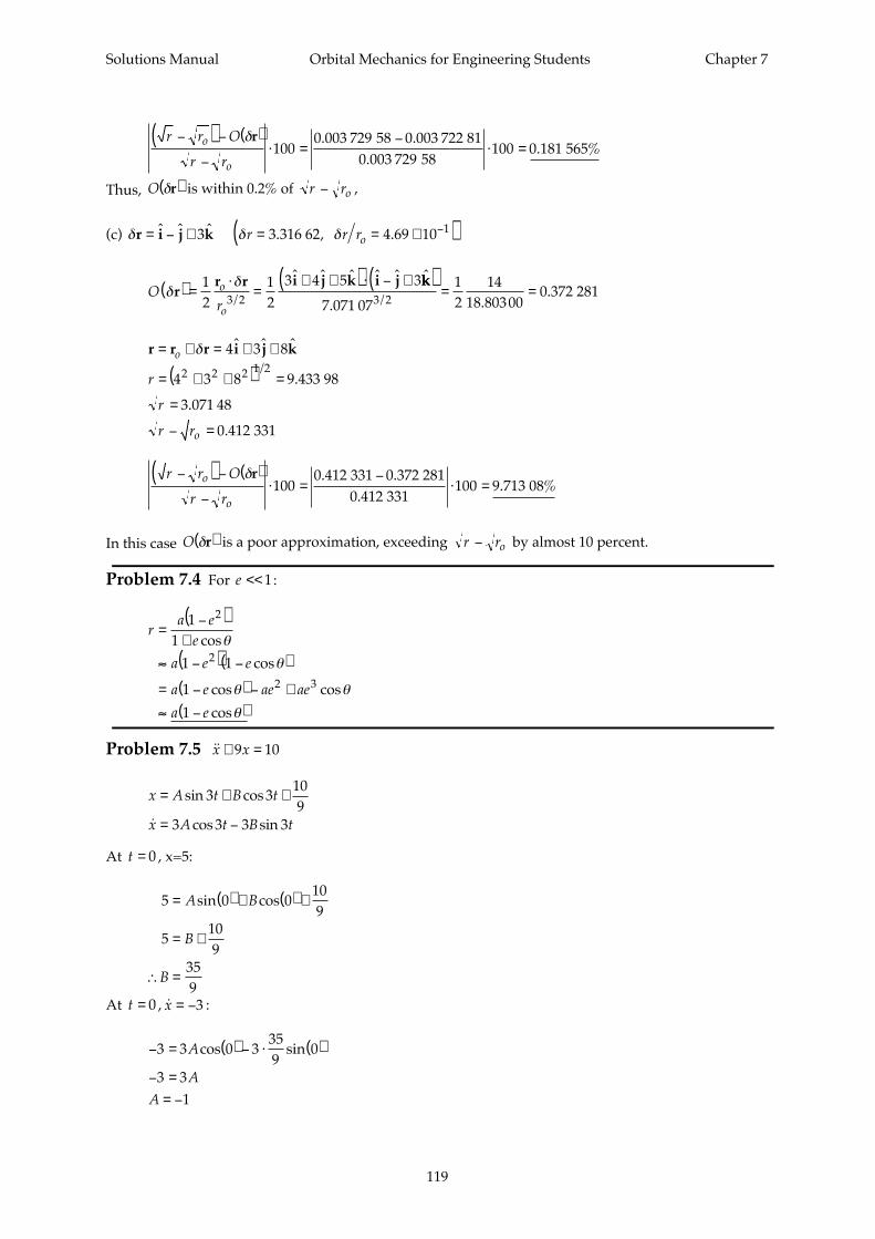
Solutions Manual Orbital Mechanics for Engineering Students Chapter 7
119
r r O
r ro
o
−( ) − ( )
−⋅ =
−⋅ =
δr100
0 003 729 58 0 003 722 810 003 729 58
100 0 181 565. .
.. %
Thus, O δr( ) is within 0.2% of r ro− ,
(c) δ δ δr i j k= − + = = ×( )−ˆ ˆ ˆ . , .3 3 316 62 4 69 10 1r r ro
Oro
o
δδ
rr r i j k i j( ) =⋅
=+ +( ) ⋅ − +1
212
3 4 5 33 2/
ˆ ˆ ˆ ˆ ˆ kk( )= =
7 071 07
12
1418 80300
0 372 2813 2. .
./
r r r i j k= + = + +o δ 4 3 8ˆ ˆ ˆ
r
r
r ro
= + +( ) =
=
− =
4 3 8 9 433 98
3 071 48
0 412 331
2 2 2 1 2/.
.
.
r r O
r ro
o
−( ) − ( )
−⋅ =
−⋅ =
δr100
0 412 331 0 372 2810 412 331
100 9 713 08. .
.. %
In this case O δr( ) is a poor approximation, exceeding r ro− by almost 10 percent.
Problem 7.4 For e << 1:
ra e
e
a e e
a e ae ae
a e
=−( )
+
≈ −( ) −( )
= −( ) − +
≈ −( )
11
1 1
1
1
2
2
2 3
cos
cos
cos cos
cos
θ
θ
θ θ
θ
Problem 7.5 x x+ =9 10
x A t B t
x A t B t
= + +
= −
sin cos
cos sin
3 3109
3 3 3 3
At t = 0 , x=5:
5 0 0109
5109
359
= ( ) + ( ) +
= +
∴ =
A B
B
B
sin cos
At t = 0 , x = −3 :
− = ( ) − ⋅ ( )
− =
= −
3 3 0 3359
0
3 31
A
A
A
cos sin
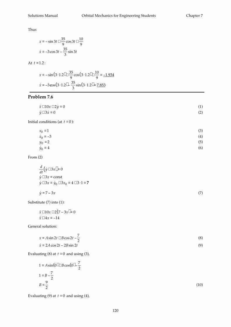
Solutions Manual Orbital Mechanics for Engineering Students Chapter 7
120
Thus
x t t
x t t
= − + +
= − −
sin cos
cos sin
3359
3109
3 3353
3
At t = 1 2. :
x
x
= − ⋅( ) + ⋅( ) + = −
= −
sin . cos . .3 1 2359
3 1 2109
1 934
3ccos . sin . .3 1 2353
3 1 2 7 853⋅( )− ⋅( ) =
Problem 7.6
x x y+ + =10 2 0 (1)
y x+ =3 0 (2)
Initial conditions (at t = 0 ):
x0 1= (3)
x0 3= − (4)
y0 2= (5)
y0 4= (6)
From (2)
ddt
y x
y x
y x y x
+( ) =
+ =
+ = + = + ⋅ =
3 0
33 3 4 3 10 0
const77
y x= −7 3 (7)
Substitute (7) into (1):
x x x
x x
+ + −( ) =
+ = −
10 2 7 3 04 14
General solution:
x A t B t= + −sin cos2 2
72
(8)
x A t B t= −2 2 2 2cos sin (9)
Evaluating (8) at t = 0 and using (3),
1 0 072
172
= ( ) + ( ) −
= −
A B
B
sin cos
B =
92
(10)
Evaluating (9) at t = 0 and using (4),
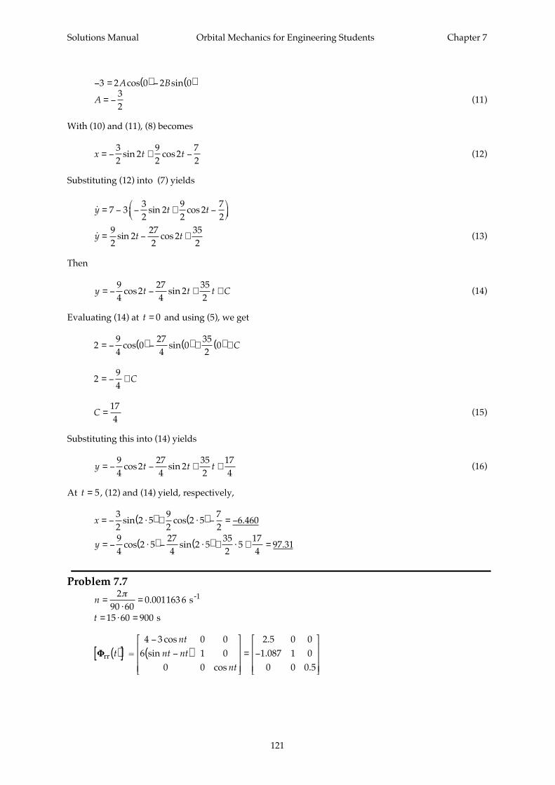
Solutions Manual Orbital Mechanics for Engineering Students Chapter 7
121
− = ( ) − ( )3 2 0 2 0A Bcos sin
A = −
32
(11)
With (10) and (11), (8) becomes
x t t= − + −
32
292
272
sin cos (12)
Substituting (12) into (7) yields
y t t= − − + −
7 332
292
272
sin cos
y t t= − +
92
2272
2352
sin cos (13)
Then
y t t t C= − − + +
94
2274
2352
cos sin (14)
Evaluating (14) at t = 0 and using (5), we get
2
94
0274
0352
0= − ( ) − ( ) + ( ) +cos sin C
2
94
= − + C
C =
174
(15)
Substituting this into (14) yields
y t t t= − − + +
94
2274
2352
174
cos sin (16)
At t = 5, (12) and (14) yield, respectively,
x
y
= − ⋅( ) + ⋅( ) − = −
= − ⋅( ) − ⋅( ) + ⋅ + =
32
2 592
2 572
6 460
94
2 5274
2 5352
5174
97 31
sin cos .
cos sin .
Problem 7.7
n
t
=⋅
=
= ⋅ =
290 60
0 001163 6
15 60 900
π. s
s
-1
ΦΦrr =t
nt
nt nt
nt( )[ ]
−
−( )
= −
4 3 0 06 1 0
0 0
2 5 0 01 087 1 0
0 0 0 5
cossin
cos
..
.
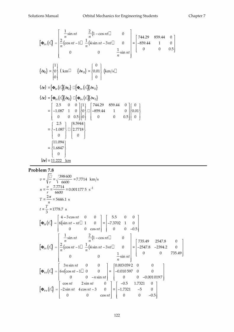
Solutions Manual Orbital Mechanics for Engineering Students Chapter 7
122
ΦΦrv =t
nnt
nnt
nnt
nnt nt
nnt
( )[ ]
−( )
−( ) −( )
= −
1 21 0
21
14 3 0
0 01
744 29 859 44 0859 44 1 0
0 0 0 5
sin cos
cos sin
sin
. ..
.
δ δr v0 0
100
00 01
0 =
( ) =
( ) . km km s
δ δ δr r v = ( )[ ] + ( )[ ] ΦΦ ΦΦrr rvt t0 0
δ δ δr r v = ( )[ ] + ( )[ ]
= −
+ −
=
ΦΦ ΦΦrr rvt t0 0
2 5 0 01 087 1 0
0 0 0 5
100
744 29 859 44 0859 44 1 0
0 0 0 5
00 01
0
2
..
.
. ..
..
...
.
.
..
.
51 087
0
8 59442 7718
0
11 0941 6847
0
11 222
−
+
=
=δr km
Problem 7.8
v
r= = =
µ 398 6006600
7 7714. km s
n
vr
= = =7 77146600
0 001177 5.
. s-1
T
n= =
25446 1
π. s
t
T= =
31778 7. s
ΦΦrr =t
nt
nt nt
nt( )[ ]
−
−( )
= −
−
4 3 0 06 1 0
0 0
5 5 0 07 3702 1 0
0 0 0 5
cossin
cos
..
.
ΦΦrv =t
nnt
nnt
nnt
nnt nt
nnt
( )[ ]
−( )
−( ) −( )
= − −
1 21 0
21
14 3 0
0 01
735 49 2547 8 02547 8 2394 2 0
0 0 735 49
sin cos
cos sin
sin
. .. .
.
ΦΦvr =t
n nt
n nt
n nt( )[ ] −( )
−
= −
−
3 0 06 1 0 0
0 0
0 003 059 2 0 00 010 597 0 0
0 0 0 0010197
sincos
sin
..
.
ΦΦvv =t
nt nt
nt nt
nt( )[ ] − −
=
−
− −
−
cos sinsin cos
cos
. ..
.
2 02 4 3 0
0 0
0 5 1 7321 01 7321 5 0
0 0 0 5
Solutions Manual Orbital Mechanics for Engineering Students Chapter 7
123
δ δ δr r vf = [ ] + [ ] +ΦΦ ΦΦrr rv0 0
000
5 5 0 07 3702 1 0
0 0 0 5
111
735 49 2547 8 02547 8 2394 2 0
0 0 735 490
= −
−
+ − −
+
..
.
. .. .
.δv
735 49 2547 8 02547 8 2394 2 0
0 0 735 49
5 5 0 07 3702 1 0
0 0 0 5
111
5 56 3702
0 50
. .. .
.
..
.
..
.− −
= − −
−
=
−
+δv
δv0
1735 49 2547 8 02547 8 2394 2 0
0 0 735 49
5 56 3702
0 5
0 000 647 340 0019718
0 000 679 82
+
−
= − −
−
=
−
−
( ). .
. ..
..
.
..
.km s
∆v v v1 0 0
0 000 647 340 0019718
0 000 679 82
00
0 005
0 000 647 340 00197180 004 320 2
= − =
−
−
−
=
−
−
−
( )+ −δ δ
..
. .
...
km s
∆ ∆v1 1 0 004792 8= =v . km s
δ δ δv r vf
− + = [ ] + [ ] ΦΦ ΦΦvr vv0 0
δv f− = −
−
+
−
− −
−
−
−
0 003 059 2 0 00 010 597 0 0
0 0 0 0010197
111
0 5 1 7321 01 7321 5 0
0 0 0 5
0 000 647 340 0019718
0 000 679 82
..
.
. ..
.
..
.
δv f− = −
−
+
−
−
0 003 059 20 010 5970 0010197
0 003 09170 010 98
0 000 339 91
...
..
.
δv f− =
−
−
( )0 000 032 48
0 000 383120 001359 6
..
. km s
δv f+ =
000
∆v v v2
000
0 000 032 480 000 38312
0 001359 6
0 000 032 480 000 383120 001359 6
= − =
−
−
−
= −
( )+ −δ δf f
..
.
...
km s
∆ ∆v2 2 0 001413= =v . km s
v v vtotal . . . . = + = + = =∆ ∆1 2 0 004792 8 0 001413 0 006 2058 6 206 km s m s
Problem 7.9
tT
ntT
=
= =
0
0
22π
π
ΦΦrr =t
nt
nt nt
nt( )[ ]
−
−( )
= −
−
4 3 0 06 1 0
0 0
7 0 06 1 00 0 1
cossin
cosπ
Solutions Manual Orbital Mechanics for Engineering Students Chapter 7
124
ΦΦrv =t
nnt
nnt
nnt
nnt nt
nnt
n
n n( )[ ]
−( )
−( ) −( )
= − −
1 21 0
21
14 3 0
0 01
04
0
4 30
0 0 0
sin cos
cos sin
sin
π
ΦΦvr =t
n nt
n nt
n nt
n( )[ ] −( )−
= −
3 0 06 1 0 0
0 0
0 0 012 0 00 0 0
sincos
sin
cos sin
sin coscos
ΦΦvv =t
nt nt
nt nt
nt( )[ ] − −
=
−
−
−
2 02 4 3 0
0 0
1 0 00 7 00 0 1
(a)
δ δ δr r vf = [ ] + [ ] +ΦΦ ΦΦrr rv0 0
000
7 0 06 1 00 0 1 0
04
0
4 30
0 0 0
0
00 0
= −
−
+ − −
π
δρ
δπ
δy
n
n nv
000
76
0
4
3
00
0
0
= − +
+ −
δρ
πδρ δ
δ
πδy
vn
vn
74
63
0
000
0
00
δρδ
πδρπδ
δ
+
− − +
=
vnv
ny
7
40
74
00δρ
δδ δρ+ = ⇒ = −
vn
v n
δ πδρ
πδρ πδρy
nn0 6
3 74
34
= + −
=
∴ =
= −
+δ
δρ
πδρ δ δρr v0 034
0
074
0
v
(b)
δ δ δv r vf
− + = [ ] + [ ] ΦΦ ΦΦvr vv0 0
δ
δρ
πδρ δρv f n v− = −
+
−
−
−
−
0 0 012 0 00 0 0
34
0
1 0 00 7 00 0 1
074
0
δ δρ δρ δρπδρ
v f n n nT
− = −
+
=
=
012
0
0494
0
014
0
012
00
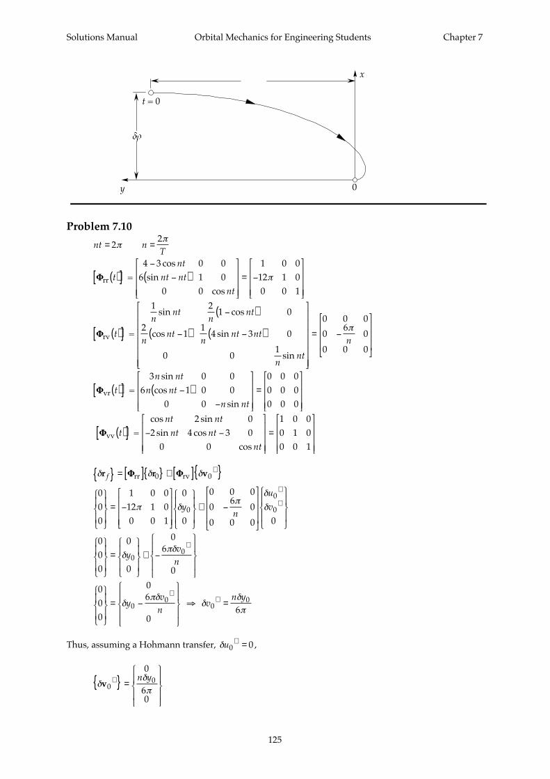
Solutions Manual Orbital Mechanics for Engineering Students Chapter 7
125
Problem 7.10
nt n
T= =2
2π
π
ΦΦrr =t
nt
nt nt
nt( )[ ]
−
−( )
= −
4 3 0 06 1 0
0 0
1 0 012 1 00 0 1
cossin
cosπ
ΦΦrv =t
nnt
nnt
nnt
nnt nt
nnt
n( )[ ]
−( )
−( ) −( )
= −
1 21 0
21
14 3 0
0 01
0 0 0
06
0
0 0 0
sin cos
cos sin
sin
π
ΦΦvr =t
n nt
n nt
n nt( )[ ] −( )
−
=
3 0 06 1 0 0
0 0
0 0 00 0 00 0 0
sincos
sin
cos sin
sin coscos
ΦΦvv =t
nt nt
nt nt
nt( )[ ] − −
=
2 02 4 3 0
0 0
1 0 00 1 00 0 1
δ δ δr r vf = [ ] + [ ] +ΦΦ ΦΦrr rv0 0
000
1 0 012 1 00 0 1
0
0
0 0 0
06
0
0 0 0 00
0
0
= −
+ −
+
+π δπ
δ
δyn
u
v
000
0
0
06
00
0
=
+ −
+
δπδ
yv
n
000
06
060
00
0
= −
⇒ =+
+δπδ
δδπ
yv
nv
n y
Thus, assuming a Hohmann transfer, δu0 0+ = ,
δδπ
v00
0
60
+ =
n y
0y
x
34πδρ
t = 0
Solutions Manual Orbital Mechanics for Engineering Students Chapter 7
126
∆
∆ ∆
v v v
v
1 0 00 0
1 10
0
60
000
0
60
6
= − =
−
=
= =
+ −δ δδπ
δπ
δπ
n y n y
vn y
δ δ δv r vf
− + = [ ] + [ ] ΦΦ ΦΦvr vv0 0
δ δδπ
v f yn y− =
+
0 0 00 0 00 0 0
0
0
1 0 00 1 00 0 1
0
60
00
δδπ
v fn y− =
0
60
0
∆v v v20 0
000
0
60
0
60
= − =
−
= −
+ −δ δδπ
δπf f
n y n y
∆ ∆v
n y2 2
06
= =vδπ
∆ ∆ ∆v v v
n y n y n y yTtotal = + = + = =1 2
0 0 0 06 6 3
23
δπ
δπ
δπ
δ
Problem 7.11
n
t
nt
=⋅
=
= ⋅ =
=
22 3600
0 000 872 66
30 60 1800
2
π
π
. s
s
-1
ΦΦrr = =t
nt
nt nt
nt( )[ ]
−
−( )
−
4 3 0 06 1 0
0 0
4 0 03 425 1 0
0 0 0
cossin
cos.
ΦΦrv = =t
nnt
nnt
nnt
nnt nt
nnt
( )[ ]
−( )
−( ) −( )
− −
1 21 0
21
14 3 0
0 01
1146 2292 02292 816 3 00 0 1146
sin cos
cos sin
sin
.
ΦΦvr = =t
n nt
n nt
n nt( )[ ] −( )
−
−
−
3 0 06 1 0 0
0 0
0 002 618 0 00 005236 0 0
0 0 0 000 8727
sincos
sin
..
.
x
yy0
y0t = 0
Solutions Manual Orbital Mechanics for Engineering Students Chapter 7
127
cos sin
sin coscos
ΦΦvv =t
nt nt
nt nt
nt( )[ ] − −
= − −
2 02 4 3 0
0 0
0 2 02 3 0
0 0 0
δ δ δr r vf = [ ] + [ ] +ΦΦ ΦΦrr rv0 0
δr f = −
+ − −
−
4 0 03 425 1 0
0 0 0
060
1146 2292 02292 816 3 00 0 1146
00 003
0. . .
δr f =
+
−
=
−
( )060
6 8752 449
0
6 8758 449
0
..
.. km
δr f = 10 89. km
δ δ δv r vf = [ ] + [ ] +ΦΦ ΦΦvr vv0 0
δv f = −
−
+ − −
−
0 002 618 0 00 005236 0 0
0 0 0 000 8727
060
0 2 02 3 0
0 0 0
00 003
0
..
..
δv f =
+
−
=
+
−
( )000
0 0060 009
0
000
0 0060 009
0
..
.. km s
δv f = 0 010 82. km s
Problem 7.12 Use C-W frame attached to original location of satellite in GEO.
n =
+
⋅= × −
22
365 2624 3600
7 292 10 5π
π. . s-1
First determine the relative position and velocity after two hours.
t
nt
= ⋅ =
=
2 3600 72000 1671
s. π
0
-6
-4
-2
2468
x (km)
y (km) t = 0
t = 30 min
Solutions Manual Orbital Mechanics for Engineering Students Chapter 7
128
ΦΦ
ΦΦ
ΦΦ
rr
rv
vr
=
=
=
tnt
nt nt
t nnt
nnt
nnt
nnt nt
t
( )[ ]−
−( )
=
−
( )[ ]−( )
−( ) −( )
=−
( )[ ]
4 3 06 1
1 404 00 1427 1
1 21
21
14 3
6874 36943694 5895
cossin
.
.
sin cos
cos sin
33 06 1 0
10 97 10 05 893 10 0
22 4 3
0 8653 1 0021 002 0 4612
5
5n nt
n nt
tnt nt
nt nt
sincos
..
cos sin
sin cos. .
. .
−( )
=
×
− ×
( )[ ]− −
=
−
−
−
ΦΦvv =
δ δ δr r v2 0 0 = [ ] + [ ] ΦΦ ΦΦrr rv
−
=−
+−
1010
1 404 00 1427 1
00
6874 36943694 5895 0
.
.δv
6874 36943694 5895
10100−
=
−
δv
δv0
16874 36943694 5895
1010
0 001770 000 587
=−
−
=
−
( )− .
.km s
δ δ δ
δ
δ
v r v
v
v
2 0 0
2
5
5
2
10 97 10 05 893 10 0
00
0 8653 1 0021 002 0 4612
0 001770 000 587
0 000 943 40
−
−−
−
−
= [ ] + [ ]
=×
− ×
+−
−
=−
ΦΦ ΦΦvr vv
..
. .. .
..
.
..
002 045
( )km s
Initiate rendezvous with the origin.
t
nt
= ⋅ =
=
6 3600 216000 5014
s. π
δ δ δ
δ
δ
r r v
v
v
6 2 2
2
2
00
4 013 03 451 1
1010
13710 27 54027 540 9947
13710 27 54027 540 9947
4 013 03 451 1
= [ ] + [ ]
=−
−
+− −
− −
= −
−
+
+
+
ΦΦ ΦΦrr rv
..
..
−
− −
=
−
=− −
−
=
( )
+
+−
1010
13710 27 54027 540 9947
40 1344 51
13710 27 54027 540 9947
40 1344 51
0 0013290 0007954
2
2
1
δ
δ
v
v
..
..
..
km s
δ δ δ
δ
δ
v r v
v
v
6 0 2
6
6
0 000 218 8 00 000 439 4 0
1010
0 004 3 22 3 017
0 0013290 0007954
0 0021880 004 394
− +
−
−
= [ ] + [ ]
=−
−
+−
− −
=−
ΦΦ ΦΦvr vv
..
..
..
..
+−
=−
−
( )0 001 5850 005057
0 000 602 50 000 663
..
..
km s
Solutions Manual Orbital Mechanics for Engineering Students Chapter 7
129
∆
∆ ∆
v v v
v
2 2 2
2 2
0 0013290 0007954
0 000 943 40 002 045
0 002 2720 001 25
0 002 593
= − =
−
−
=−
( )
= =
+ −δ δ.
...
..
.
km s
km sv
∆v v v6 6 6
00
0 000 602 50 000 663
0 000 602 50 000 663
= − =
−
−
−
=
( )+ −δ δ..
..
km s
∆ ∆v6 6 0 000 8958= =v . km s
∆ ∆ ∆v v vtotal = + = + = =2 6 0 002 593 0 000 8958 0 003 489 3 489. . . . km s m s
Problem 7.13 Design problem.
Problem 7.14
n
v n x
= =
= − = − ⋅ ⋅ = =
398 6006600
66000 001 177 5
32
32
0 001 177 5 5 0 008 8311 8 8311
.
. . .
s
km s m s
-1
δ δ
Problem 7.15
nt =
π2
ΦΦ
ΦΦ
rr
rv
=
=
tnt
nt nt
t nnt
nnt
nnt
nnt nt
n n
n n
( )[ ]−
−( )
=
−
( )[ ]−( )
−( ) −( )
=− −
4 3 06 1
4 03 425 1
1 21
21
14 3
1 2
2 0 7124
cossin .
sin cos
cos sin.
δ δ δr r vf = [ ] + [ ] ΦΦ ΦΦrr rv0 0
δδ
πδ
πδ
δr f
r
rn n
n n
n r
n r =−
+− −
−
4 03 425 1
1 2
2 0 7124167
4. .
δ
δ
δ
δ
δ
δ
δr f
r
r
r
r
r
r =−
+−
=
40 2832
3 3040 854
0 69630 85708.
..
..
246810
-8
-6
-4
-2
0
x (km)
y (km)t = 0
t = 2 hr
Outbound
Return
-10
Solutions Manual Orbital Mechanics for Engineering Students Chapter 7
130
d rf= =δ δr 0 9004.
Problem 7.16 nt = π nt = π
ΦΦ
ΦΦ
rr
rv
=
=
tnt
nt nt
t nnt
nnt
nnt
nnt nt
n
n n
( )[ ]−
−( )
=
−
( )[ ]−( )
−( ) −( )
=− −
4 3 06 1
7 018 85 1
1 21
21
14 3
04
4 9 425
cossin .
sin cos
cos sin.
δ δ δ
δδ
r r v
v
f
x n
n n
= [ ] + [ ]
=−
+− −
ΦΦ ΦΦrr rv0 0
00
00
7 018 85 1 0
04
4 9 425. .
04
4 9 4257
18 85
04
4 9 4257
18 85
0 5891 75
00
0
0
1
0
0
00
0
n
n n
x
x
n
n n
x
x
n x
n x
− −
=
−
=− −
−
=−
−
−
. .
. .
..
δδ
δ
δδ
δ
δδ
δ
v
v
v
or
δ δ δv i j0 0 00 589 1 75= − − ( ). ˆ . ˆ n x n x km s
Problem 7.17
nt =
π4
ΦΦ
ΦΦ
rr
rv
=
=
tnt
nt nt
t nnt
nnt
nnt
nnt nt
n n
n n
( )[ ]−
−( )
=
−
( )[ ]−( )
−( ) −( )
=−
4 3 06 1
1 879 00 4697 1
1 21
21
14 3
0 7071 0 5858
0 5858 0 4722
cossin
.
.
sin cos
cos sin
. .
. .
δ δ δr r vf = [ ] + [ ] ΦΦ ΦΦrr rv0 0
00
1 879 00 4697 1
0 7071 0 5858
0 5858 0 47220
0 0
=−
−
+−
.
.
. .
. .d
yn n
n nvδ δ
00
1 8790 4697
0 5858
0 47220
0
0
=−
+
+
..
.
.d
d y
vn
vn
δ
δ
δ
0 58581 879
0 47220 4697
00
0
00
..
..
δ
δδ
vn
d
vn
d y
−
+ +
=
Solutions Manual Orbital Mechanics for Engineering Students Chapter 7
131
00 5858
10 4722
1 8790 4697
0
0
.
...
n
n
y
v
d
d
=−
δ
δ
δ
δ
δ
δ
y
vn
n
d
d
y
v n
d
d
d
nd
0
0
1
0
0
00 5858
10 4722
1 8790 4697
0 8062 11 707 0
1 8790 4697
1 9843 207
=
−
=−
−
=−
−.
...
..
.
..
.
δy d0 1 984= − .

Solutions Manual Orbital Mechanics for Engineering Students Chapter 7
132
Solutions Manual Orbital Mechanics for Engineering Students Chapter 8
133
Problem 8.1
µ
µ
sun3 2
earth3 2
earth
earth
km s
km s
km km
= ×
=
= ×
=
132 7 10
398 600
147 4 106378
9
6
.
. R
r
a R R=
12
12
kmearth +( ) = × + ×( ) = ×26 6 6147 4 10 120 10 138 7 10. .
Heliocentric spacecraft velocity at earth’s sphere of influence:
V
R av( ) = −
= ×
×−
×
=µsun
earthkm s
2 1132 7 10
2
147 4 10
1
138 7 1028 439
6 6.. .
.
Heliocentric velocity of earth:
V
Rearthsun
earthkm s= =
×
×=
µ 132 7 10
149 6 1030 06
9
6.
..
∴ = − = − =∞( )v V V v
earth km s30 06 28 43 1 579. . .
Geocentric spacecraft velocity of spacecraft at perigee of departure hyperbola:
v v
rpp
= + = +⋅
+=∞
2 221 579
2 398 6006378 200
11 12µearth km s. .
Geocentric spacecraft velocity in its circular parking orbit:
v
rc = =+
=µearth
km s398 600
6378 2007 784.
∴ = − = − =∆v v vp c 11 12 7 784 3 337. . . km s
Problem 8.2
µ
µ
µ
sun3 2
earth3 2
Mercury3 2
km s
km s
km s
= ×
=
=
132 7 10
398 600
22 930
9.
R
R
earth
Mercury
km
km
= ×
= ×
149 6 10
57 91 10
6
6
.
.
r
rearth
Mercury
km km
=
=
63782440
V
Rearthsun
earthkm s= =
×
×=
µ 132 7 10
149 6 1029 78
9
6.
..
V
RMercurysun
Mercurykm s= =
×
×=
µ 132 7 10
57 91 1047 87
9
6.
..
Solutions Manual Orbital Mechanics for Engineering Students Chapter 8
134
Semimajor axis of Hohmann transfer ellipse:
a R R=
12
12
kmearth Mercury+( ) = × + ×( ) = ×149 6 10 57 91 10 103 8 106 6 6. . .
Departure from earth:
Spacecraft heliocentric velocity:
V
R av( ) = −
= ×
×−
×
=µsun
earthkm s
2 1132 7 10
2
149 6 10
1
103 8 1022 259
6 6.. .
.
∴ = − = − =∞( )v V V v
earth km s29 78 22 25 7 532. . .
Spacecraft geocentric velocity in circular parking orbit:
v
rcp
= =+
=µearth km s
398 6006378 150
7 814.
Spacecraft geocentric velocity at perigee of departure hyperbola:
v v
rpp
= + = +⋅
+=∞
2 227 532
2 398 6006378 150
13 37µearth km s. .
∴ = − = − =∆v v vp c1 13 37 7 814 9 611. . . km s
Arrival at Mercury:
Spacecraft heliocentric velocity:
VR a
v( ) = −
= ×
×−
×
= .
. ..µsun
Mercurykm s
2 1132 7 10
2
57 91 10
1
103 8 1057 489
6 6
∴ = − = − =∞
( )v V VvMercury km s57 48 47 87 9 611. . .
Spacecraft velocity relative to Mercury at periapse of approach hyperbola:
v v
rpp
= + = +⋅
+=∞
2 229 611
2 22 9302440 150
10 49µMercury
km s. .
Spacecraft parking orbit speed relative to Mercury:
v
rcp
= =+
=µMercury
km s22 930
2440 1502 975.
∴ = − = − =∆v v vp c2 10 49 2 975 7 516. . . km s
∆ ∆ ∆v v vtotal = + = + =1 2 9 611 7 516 15 03. . . km s
Problem 8.3
r Rm
m
m
SOIp
=
= ×
sun
sun kg1 989 1030.
Mercury:
Solutions Manual Orbital Mechanics for Engineering Students Chapter 8
135
R
m
r
p
SOI
= 57.91 10 km
kg
57.91 10 km
6
6
×
= ×
= ××
×
= ×
.
.
..
3 302 10
3 302 10
1 989 101 124 10
23
23
305
Venus:
R
m
r
p
SOI
= 108.2 10 km
kg
108.2 10 km
6
6
×
= ×
= ××
×
= ×
.
.
..
4 869 10
4 869 10
1 989 106 162 10
24
24
305
Mars:
R
m
r
p
SOI
= 227.9 10 km
kg
227.9 10 km
6
6
×
= ×
= ××
×
= ×
.
.
..
6 419 10
6 419 10
1 989 105 771 10
23
23
305
Jupiter:
R
m
r
p
SOI
= 778.6 10 km
kg
778.6 10 km
6
6
×
= ×
= ××
×
= ×
.
.
..
1 899 10
1 899 10
1 989 104 882 10
27
27
307
Problem 8.4
r Rm
m
m
SOIp
=
= ×
sun
sun kg1 989 1030.
Saturn:
R
m
r
p
SOI
= 1433 10 km
kg
1433 10 km
6
6
×
= ×
= ××
×
= ×
.
.
..
5 685 10
5 685 10
1 989 105 479 10
26
26
307
Uranus:
R
m
r
p
SOI
= 2872 10 km
kg
2872 10 km
6
6
×
= ×
= ××
×
= ×
.
.
..
8 683 10
8 683 10
1 989 105 178 10
25
25
307
Neptune:
R
m
r
p
SOI
= 4495 10 km
kg
km
6×
= ×
= ××
×
= ×
.
..
..
1 024 10
1 024 101 024 10
1 989 108 658 10
26
2626
307

Solutions Manual Orbital Mechanics for Engineering Students Chapter 8
136
Pluto:
R
m
r
p
SOI
= 5870 10 km
kg
5870 10 km
6
6
×
= ×
= ××
×
= ×
.
.
..
1 25 10
1 25 10
1 989 103 076 10
22
22
306
Problem 8.5
µ
µ
sun3 2
Jupiter3 2
earth
Jupiter
Jupiter
km s
km s
km
km
km
= ×
= ×
= ×
= ×
=
132 7 10
126 7 10
149 6 10
778 6 10
71490
9
6
6
6
.
.
.
.
R
R
r
Semimajor axis of Hohmann transfer ellipse:
a R R1
6 6 612
12
149 6 10 778 6 10 464 1 10= +( ) = × + ×( ) = ×earth Jupiter km. . .
V
RJupitersun
Jupiterkm s= =
×
×=
µ 132 7 10
778 6 1013 06
9
6.
..
Use the energy equation to obtain the spacecraft’s velocity upon arrival at Jupiter’s sphere ofinfluence:
VR a
v1
1
96 6
2 1132 7 10
2
778 6 10
1
464 1 107 412( ) = −
= ×
×−
×
=µsun
Jupiter km s.
. ..
v V V v∞
( )= − = − =Jupiter km s1 13 06 7 412 5 643. . .
Eccentricity of hyperbolic swing by trajectory:
e
r vp= + = +
⋅
×=
∞1 1
271490 5 643
126 7 101 068
2 2
6µJupiter
.
. .
Turn angle:
δ =
=
= °− −2
12
11 068
138 81 1sin sin.
.e
Angle between VJupiter and v∞ at inbound crossing: φ1 180= ° . At the outbound crossing,
VJupiter = 13.06 km/s 149.6(106) km
778.6(106) km
Sun
uV
uS
V1v 7.412 km s

Solutions Manual Orbital Mechanics for Engineering Students Chapter 8
137
v 1
v 2 uV
uS
318.8°
v 1
v 2
V v
p
φ δ2 180 318 8= ° + = °.
At the outbound crossing
V V v
u u
2 2
2
v
V VV v v
( )∞
∞
= +
= + +
Jupiter
Jupiter ˆ cos ˆφ ∞∞( )= + ⋅ ° +
sin ˆ
. ˆ . cos . ˆ .
φ2
13 06 5 643 318 8 5
u
u u
S
V V 6643 318 8
17 30 3 716
sin . ˆ
. ˆ . ˆ
°( )= − ( )
u
u uS
V S km s
∆V V V
u u
v v v
V S
( ) ( ) ( )= −
= −( ) −2 1
17 30 3 716 7 412. ˆ . ˆ . ˆ
. ˆ . ˆ
u
u uV
V S= − ( )9 890 3 716 km s
∴ = =( ) ( )∆ ∆V v vV 10 57. km s
Alternatively, ∆V vv( )
∞= = ⋅ ⋅°
=22
2 5 643138 8
210 57sin . sin
..
δkm s.
Angular momentum of the new orbit after flyby:
h R V v
26 9778 6 10 17 30 13 47 10= = × ⋅ = ×⊥
( )Jupiter
2 km s. . .
Obtain the semimajor axis a2 from the energy equation:
VR a
v2
2
22 2
( )− = −
µ µsun
Jupiter
sun
17 702
132 7 10
778 6 10
132 7 102
4 791 102 9
6
9
22
9. .
.
. . −
×
×= −
×⇒ = ×
aa km
Observe that a a2 1 10 32= . . The new orbit dwarfs the original one in size and, therefore, energy.
Use Equation 3.61 to find the eccentricity:
ah
e
ee
22
2
22
992
92
2 2
1
1
4 791 1013 47 10
132 7 10
1
10 8453
=−
× =×
× −⇒ =
µsun
..
. .
Use the orbit equation to find the true anomaly in the new orbit:
R
heJupiter
sun=
+2
2
2 2
11µ θcos
778 6 10
13 47 10
132 7 10
11 0 8453
26 5692
92
2..
. . cos .× =
×
× +⇒ = °
θθ
The new and original heliocentric orbits are illustrated below.
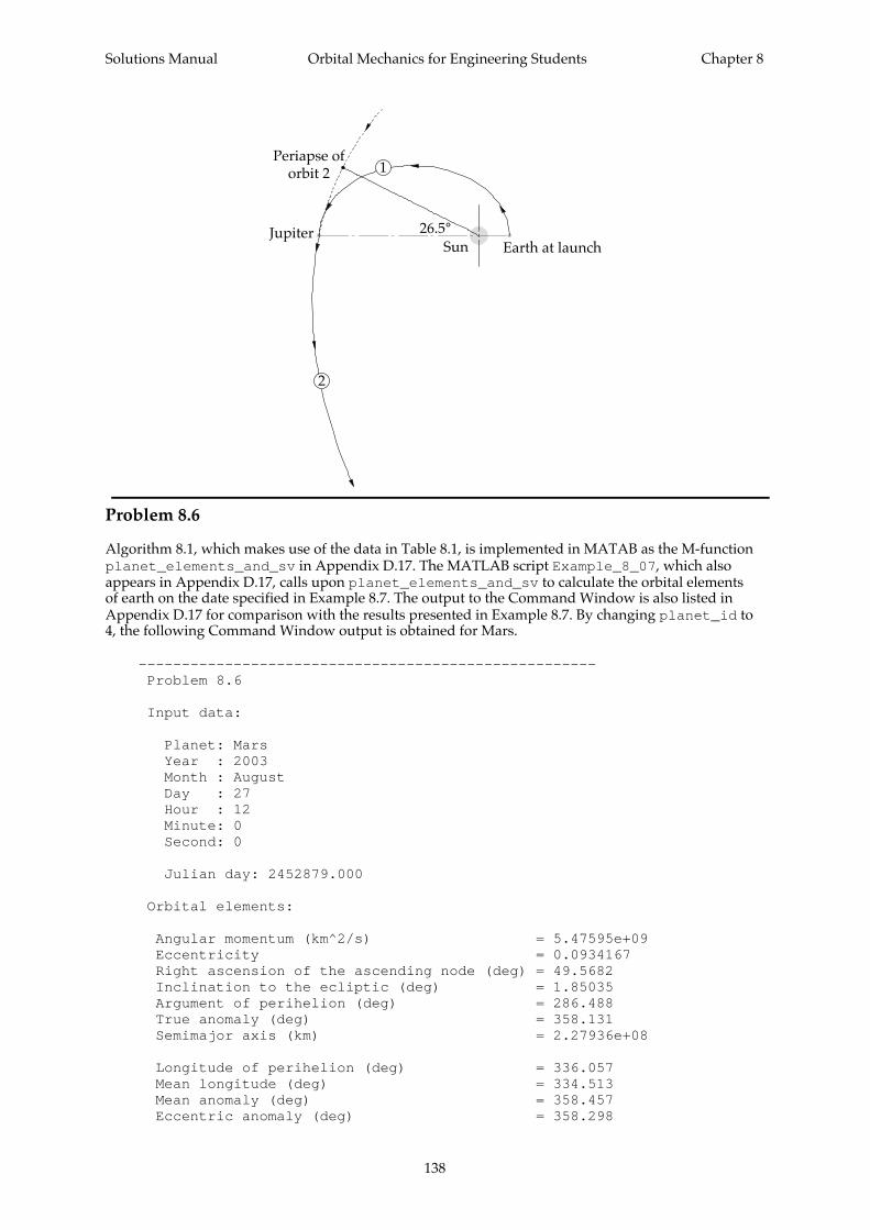
Solutions Manual Orbital Mechanics for Engineering Students Chapter 8
138
Problem 8.6
Algorithm 8.1, which makes use of the data in Table 8.1, is implemented in MATAB as the M-functionplanet_elements_and_sv in Appendix D.17. The MATLAB script Example_8_07, which alsoappears in Appendix D.17, calls upon planet_elements_and_sv to calculate the orbital elementsof earth on the date specified in Example 8.7. The output to the Command Window is also listed inAppendix D.17 for comparison with the results presented in Example 8.7. By changing planet_id to4, the following Command Window output is obtained for Mars.
----------------------------------------------------- Problem 8.6
Input data:
Planet: Mars Year : 2003 Month : August Day : 27 Hour : 12 Minute: 0 Second: 0
Julian day: 2452879.000
Orbital elements:
Angular momentum (km^2/s) = 5.47595e+09 Eccentricity = 0.0934167 Right ascension of the ascending node (deg) = 49.5682 Inclination to the ecliptic (deg) = 1.85035 Argument of perihelion (deg) = 286.488 True anomaly (deg) = 358.131 Semimajor axis (km) = 2.27936e+08
Longitude of perihelion (deg) = 336.057 Mean longitude (deg) = 334.513 Mean anomaly (deg) = 358.457 Eccentric anomaly (deg) = 358.298
1
2
SunJupiter
Earth at launch
Periapse oforbit 2
26.5°
Solutions Manual Orbital Mechanics for Engineering Students Chapter 8
139
State vector:
Position vector (km) = [1.85954e+08 -8.99155e+07 -6.45661e+06] Magnitude = 2.06653e+08
Velocity (km/s) = [11.4744 23.8842 0.218255] Magnitude = 26.4984-----------------------------------------------------
Problem 8.7 The following MATLAB script calls upon Algorithm 8.1, implemented as theMATLAB M-function planet_elements_and_sv in Appendix D.17, to compute the distance of theearth from the sun on the first day of each month of the year 2005, at 12:00:00 UT. The output to theMATLAB command window is listed afterwards.
% ~~~~~~~~~~~~~~~~~~~~~~~~~~~~~~~~~~~~~~~~~~~~~~~~~~~~~~~~~~~~~~~~~~~~% Problem_8_07a% ~~~~~~~~~~~~~%% This program uses Algorithm 8.1 to compute the orbital elements% and state vector of Mars at the date and time specified% in Example 8.7.%% mu - gravitational parameter of the sun (km^3/s^2)%% coe - vector of heliocentric orbital elements% [h e RA incl w TA a w_hat L M E],% where% h = angular momentum (km^2/s)% e = eccentricity% RA = right ascension (deg)% incl = inclination (deg)% w = argument of perihelion (deg)% TA = true anomaly (deg)% a = semimajor axis (km)% w_hat = longitude of perihelion ( = RA + w) (deg)% L = mean longitude ( = w_hat + M) (deg)% M = mean anomaly (deg)% E = eccentric anomaly (deg)%% r - heliocentric position vector (km)% v - heliocentric velocity vector (km/s)%% planet_id - planet identifier:% 1 = Mercury% 2 = Venus% 3 = Earth% 4 = Mars% 5 = Jupiter% 6 = Saturn% 7 = Uranus% 8 = Neptune% 9 = Pluto%% year - range: 1901 - 2099% month - range: 1 - 12% day - range: 1 - 31% hour - range: 0 - 23% minute - range: 0 - 60% second - range: 0 - 60%% User M-functions required: planet_elements_and_sv,% month_planet_names
Solutions Manual Orbital Mechanics for Engineering Students Chapter 8
140
% --------------------------------------------------------------------
global mumu = 1.327124e11;deg = pi/180;
%...Data declaration for Problem 8.6 :planet_id = 3;year = 2005;day = 1;hour = 12;minute = 0;second = 0;%...
fprintf('\n-----------------------------------------------------\n')fprintf(' Problem 8.7a: Determine the month\n')fprintf('\n Year = %g Time = 12:00:00 UT\n', year)
for month = 1:12 %...Algorithm 8.1: [coe, r, v, jd] = planet_elements_and_sv ... (planet_id, year, month, day, hour, minute, second); %...Convert the month numbers into names for output: [month_name, planet_name] = month_planet_names(month, planet_id); fprintf('\n %10s 1st: Distance = %11.5e (km)', month_name,norm(r))endfprintf('\n-----------------------------------------------------\n')
----------------------------------------------------- Problem 8.7a: Determine the month
Year = 2005 Time = 12:00:00 UT
January 1st: Distance = 1.47100e+08 (km) February 1st: Distance = 1.47417e+08 (km) March 1st: Distance = 1.48243e+08 (km) April 1st: Distance = 1.49505e+08 (km) May 1st: Distance = 1.50745e+08 (km) June 1st: Distance = 1.51707e+08 (km) July 1st: Distance = 1.52093e+08 (km) August 1st: Distance = 1.51830e+08 (km) September 1st: Distance = 1.50963e+08 (km) October 1st: Distance = 1.49758e+08 (km) November 1st: Distance = 1.48464e+08 (km) December 1st: Distance = 1.47505e+08 (km)-----------------------------------------------------
This list reveals that the greatest distance occurs in the month of July. We can modify the aboveMATLAB script to loop through the days of July:
% ~~~~~~~~~~~~~~~~~~~~~~~~~~~~~~~~~~~~~~~~~~~~~~~~~~~~~~~~~~~~~~~~~~~~% Problem_8_07b% ~~~~~~~~~~~~~%% This program uses Algorithm 8.1 to determine the distance of the% earth from the sun, according to Problem 8.7%% User M-functions required: planet_elements_and_sv,% month_planet_names% --------------------------------------------------------------------
Solutions Manual Orbital Mechanics for Engineering Students Chapter 8
141
global mumu = 1.327124e11;
%...Data declaration for Problem 8.7 :planet_id = 3;year = 2005;month = 7;hour = 12;minute = 0;second = 0;%...
fprintf('\n-----------------------------------------------------\n')fprintf(' Problem 8.7b: Determine the day\n')fprintf('\n Year = %g Time = 12:00:00 UT\n', year)%...Convert the planet_id and month numbers into names for output:
[month_name, planet_name] = month_planet_names(month, planet_id);
for day = 1:31 %...Algorithm 8.1: [coe, r, v, jd] = planet_elements_and_sv ... (planet_id, year, month, day, hour, minute, second); %...Convert the planet_id and month numbers into names for output: [month_name, planet_name] = month_planet_names(month, planet_id); fprintf('\n %5s %4g: Distance = %14.7e (km)',...
month_name, day, norm(r))endfprintf('\n-----------------------------------------------------\n')
The output to the MATLAB command window is:
----------------------------------------------------- Problem 8.7b: Determine the day
Year = 2005 Time = 12:00:00 UT
July 1: Distance = 1.5209314e+08 (km) July 2: Distance = 1.5209524e+08 (km) July 3: Distance = 1.5209664e+08 (km) July 4: Distance = 1.5209732e+08 (km) July 5: Distance = 1.5209728e+08 (km) July 6: Distance = 1.5209653e+08 (km) July 7: Distance = 1.5209506e+08 (km) July 8: Distance = 1.5209287e+08 (km) July 9: Distance = 1.5208998e+08 (km) July 10: Distance = 1.5208637e+08 (km) July 11: Distance = 1.5208204e+08 (km) July 12: Distance = 1.5207701e+08 (km) July 13: Distance = 1.5207126e+08 (km) July 14: Distance = 1.5206481e+08 (km) July 15: Distance = 1.5205765e+08 (km) July 16: Distance = 1.5204978e+08 (km) July 17: Distance = 1.5204122e+08 (km) July 18: Distance = 1.5203195e+08 (km) July 19: Distance = 1.5202198e+08 (km) July 20: Distance = 1.5201132e+08 (km) July 21: Distance = 1.5199996e+08 (km) July 22: Distance = 1.5198792e+08 (km) July 23: Distance = 1.5197519e+08 (km) July 24: Distance = 1.5196178e+08 (km) July 25: Distance = 1.5194769e+08 (km) July 26: Distance = 1.5193292e+08 (km)

Solutions Manual Orbital Mechanics for Engineering Students Chapter 8
142
July 27: Distance = 1.5191748e+08 (km) July 28: Distance = 1.5190138e+08 (km) July 29: Distance = 1.5188461e+08 (km) July 30: Distance = 1.5186718e+08 (km) July 31: Distance = 1.5184910e+08 (km)-----------------------------------------------------
The furthest distance occurs on July 4.
Problem 8.8 For the data given in this problem, the following MATLAB script invokes Algorithm8.2, which is implemented as the MATLAB M-function interplanetary in Appendix D.18.interplanetary uses Algorithms 8.1 and 5.2 to compute v∞ at the home and target planets. Theoutput to the MATLAB Command Window is listed afterwards.
% ~~~~~~~~~~~~~~~~~~~~~~~~~~~~~~~~~~~~~~~~~~~~~~~~~~~~~~~~~~~~~~~~~~~~% Problem_8_08% ~~~~~~~~~~~~%% This program uses Algorithm 8.2 to obtain v-infinities% in Problem 8.8.%% mu - gravitational parameter of the sun (km^3/s^2)% deg - conversion factor between degrees and radians% pi - 3.1415926...%% planet_id - planet identifier:% 1 = Mercury% 2 = Venus% 3 = Earth% 4 = Mars% 5 = Jupiter% 6 = Saturn% 7 = Uranus% 8 = Neptune% 9 = Pluto%% year - range: 1901 - 2099% month - range: 1 - 12% day - range: 1 - 31% hour - range: 0 - 23% minute - range: 0 - 60% second - range: 0 - 60%% depart - [planet_id, year, month, day, hour, minute, second]% at departure% arrive - [planet_id, year, month, day, hour, minute, second]% at arrival%% planet1 - [Rp1, Vp1, jd1]% planet2 - [Rp2, Vp2, jd2]% trajectory - [V1, V2]%% coe - orbital elements [h e RA incl w TA]% where% h = angular momentum (km^2/s)% e = eccentricity% RA = right ascension of the ascending% node (rad)% incl = inclination of the orbit (rad)% w = argument of perigee (rad)% TA = true anomaly (rad)
Solutions Manual Orbital Mechanics for Engineering Students Chapter 8
143
% a = semimajor axis (km)%% jd1, jd2 - Julian day numbers at departure and arrival% tof - time of flight from planet 1 to planet 2 (days)%% Rp1, Vp1 - state vector of planet 1 at departure (km, km/s)% Rp2, Vp2 - state vector of planet 2 at arrival (km, km/s)% R1, V1 - heliocentric state vector of spacecraft at% departure (km, km/s)% R2, V2 - heliocentric state vector of spacecraft at% arrival (km, km/s)%% vinf1, vinf2 - hyperbolic excess velocities at departure% and arrival (km/s)%% User M-functions required: interplanetary, coe_from_sv,% month_planet_names% --------------------------------------------------------------------
clearglobal mumu = 1.327124e11;deg = pi/180;
%...Data declaration for Problem 8.8:
%...Departureplanet_id = 3;year = 2005;month = 12;day = 1;hour = 0;minute = 0;second = 0;depart = [planet_id year month day hour minute second];
%...Arrivalplanet_id = 2;year = 2006;month = 4;day = 1;hour = 0;minute = 0;second = 0;arrive = [planet_id year month day hour minute second];
%...
%...Algorithm 8.2:[planet1, planet2, trajectory] = interplanetary(depart, arrive);
R1 = planet1(1,1:3);Vp1 = planet1(1,4:6);jd1 = planet1(1,7);
R2 = planet2(1,1:3);Vp2 = planet2(1,4:6);jd2 = planet2(1,7);
V1 = trajectory(1,1:3);V2 = trajectory(1,4:6);
tof = jd2 - jd1;
Solutions Manual Orbital Mechanics for Engineering Students Chapter 8
144
%...Use Algorithm 5.1 to find the orbital elements of the% spacecraft trajectory based on [Rp1, V1]...coe = coe_from_sv(R1, V1);% ... and [R2, V2]coe2 = coe_from_sv(R2, V2);
%...Equations 8.102 and 8.103:vinf1 = V1 - Vp1;vinf2 = V2 - Vp2;
%...Echo the input data and output the solution to% the command window:fprintf('-----------------------------------------------------')fprintf('\n Problem 8.8: Earth to Venus')fprintf('\n\n Departure:\n');fprintf('\n Planet: %s', planet_name(depart(1)))fprintf('\n Year : %g', depart(2))fprintf('\n Month : %s', month_name(depart(3)))fprintf('\n Day : %g', depart(4))fprintf('\n Hour : %g', depart(5))fprintf('\n Minute: %g', depart(6))fprintf('\n Second: %g', depart(7))fprintf('\n\n Julian day: %11.3f\n', jd1)fprintf('\n Planet position vector (km) = [%g %g %g]', ... R1(1),R1(2), R1(3))
fprintf('\n Magnitude = %g\n', norm(R1))
fprintf('\n Planet velocity (km/s) = [%g %g %g]', ... Vp1(1), Vp1(2), Vp1(3))
fprintf('\n Magnitude = %g\n', norm(Vp1))
fprintf('\n Spacecraft velocity (km/s) = [%g %g %g]', ... V1(1), V1(2), V1(3))
fprintf('\n Magnitude = %g\n', norm(V1))
fprintf('\n v-infinity at departure (km/s) = [%g %g %g]', ... vinf1(1), vinf1(2), vinf1(3))
fprintf('\n Magnitude = %g\n', norm(vinf1))
fprintf('\n\n Time of flight = %g days\n', tof)
fprintf('\n\n Arrival:\n');fprintf('\n Planet: %s', planet_name(arrive(1)))fprintf('\n Year : %g', arrive(2))fprintf('\n Month : %s', month_name(arrive(3)))fprintf('\n Day : %g', arrive(4))fprintf('\n Hour : %g', arrive(5))fprintf('\n Minute: %g', arrive(6))fprintf('\n Second: %g', arrive(7))fprintf('\n\n Julian day: %11.3f\n', jd2)fprintf('\n Planet position vector (km) = [%g %g %g]', ... R2(1), R2(2), R2(3))
fprintf('\n Magnitude = %g\n', norm(R1))
fprintf('\n Planet velocity (km/s) = [%g %g %g]', ... Vp2(1), Vp2(2), Vp2(3))
Solutions Manual Orbital Mechanics for Engineering Students Chapter 8
145
fprintf('\n Magnitude = %g\n', norm(Vp2))
fprintf('\n Spacecraft Velocity (km/s) = [%g %g %g]', ... V2(1), V2(2), V2(3))
fprintf('\n Magnitude = %g\n', norm(V2))
fprintf('\n v-infinity at arrival (km/s) = [%g %g %g]', ... vinf2(1), vinf2(2), vinf2(3))
fprintf('\n Magnitude = %g', norm(vinf2))
fprintf('\n\n\n Orbital elements of flight trajectory:\n')
fprintf('\n Angular momentum (km^2/s) = %g',... coe(1))fprintf('\n Eccentricity = %g',... coe(2))fprintf('\n Right ascension of the ascending node (deg) = %g',... coe(3)/deg)fprintf('\n Inclination to the ecliptic (deg) = %g',... coe(4)/deg)fprintf('\n Argument of perihelion (deg) = %g',... coe(5)/deg)fprintf('\n True anomaly at departure (deg) = %g',... coe(6)/deg)fprintf('\n True anomaly at arrival (deg) = %g\n',... coe2(6)/deg)fprintf('\n Semimajor axis (km) = %g',... coe(7))% If the orbit is an ellipse, output the period:if coe(2) < 1 fprintf('\n Period (days) = %g',... 2*pi/sqrt(mu)*coe(7)^1.5/24/3600)endfprintf('\n-----------------------------------------------------\n')
----------------------------------------------------- Problem 8.8: Earth to Venus
Departure:
Planet: Earth Year : 2005 Month : December Day : 1 Hour : 0 Minute: 0 Second: 0
Julian day: 2453705.500
Planet position vector (km) = [5.33243e+07 1.37541e+08 -1830.84] Magnitude = 1.47517e+08
Planet velocity (km/s) = [-28.2595 10.6564 -6.01367e-05] Magnitude = 30.202
Spacecraft velocity (km/s) = [-27.0436 6.58196 2.7931] Magnitude = 27.9729
v-infinity at departure (km/s) = [1.2159 -4.07444 2.79316]
Solutions Manual Orbital Mechanics for Engineering Students Chapter 8
146
Magnitude = 5.08735
Time of flight = 121 days
Arrival:
Planet: Venus Year : 2006 Month : April Day : 1 Hour : 0 Minute: 0 Second: 0
Julian day: 2453826.500
Planet position vector (km) = [-5.74135e+07 -9.1938e+07 2.05581e+06] Magnitude = 1.47517e+08
Planet velocity (km/s) = [29.4613 -18.7099 -1.95644] Magnitude = 34.955
Spacecraft Velocity (km/s) = [30.3918 -22.2324 -3.68154] Magnitude = 37.8351
v-infinity at arrival (km/s) = [0.930541 -3.52248 -1.7251] Magnitude = 4.0311
Orbital elements of flight trajectory:
Angular momentum (km^2/s) = 4.0914e+09 Eccentricity = 0.183291 Right ascension of the ascending node (deg) = 68.8159 Inclination to the ecliptic (deg) = 5.77973 Argument of perihelion (deg) = 142.255 True anomaly at departure (deg) = 217.738 True anomaly at arrival (deg) = 26.8913
Semimajor axis (km) = 1.30519e+08 Period (days) = 297.66-----------------------------------------------------
The output shows that at departure from earth, v∞ = 5 087. km s. Hence, the spacecraft velocity atperigee of the departure hyperbola is
v vr
pp
= + = +⋅
+( )=∞
22
22
25 087
2 398 600
6378 18012 14
µearth km s. .
The spacecraft velocity in its circular 180 km parking orbit is
v
rcp
= =+
=µearth km s
398 6006378 180
7 796.
Hence, the delta-v requirement at earth is
∆v v vp c1 12 14 7 796 4 346= − = − =. . . km s
Solutions Manual Orbital Mechanics for Engineering Students Chapter 8
147
At Venus ( µVenus3 2 km s= 324 900 , rVenus km= 6052 ) the above output shows that
v∞ = 4 031. km s . The speed at the 300 km altitude periapse on the arrival hyperbola is therefore
v vr
pp
hyperbolaVenus km s= + = +
⋅
+( )=∞
22
22
24 031
2 324 900
6052 30010 89
µ. .
The semimajor axis of the elliptical capture orbit is
a r r= +( ) + +( )[ ] =
12
300 9000 10702Venus Venus
Therefore the velocity at periapse on the ellipse is, using the energy equation,
vr appellipse Venus km s= −
=
+−
=µ
2 1324 900
26052 300
110702
8 482.
It follows that the delta-v requirement at Venus is
∆v v vp p2 10 89 8 482 2 406= − = − =
hyperbola ellipsekm s. . .
The total delta-v requirement is
∆ ∆ ∆v v vtotal = + = + =1 2 4 346 2 406 6 753. . . km s
Problem 8.9 For the data given in this problem, the following MATLAB script invokes Algorithm8.2, which is implemented as the MATLAB M-function interplanetary in Appendix D.18.interplanetary uses Algorithms 8.1 and 5.2 to compute v∞ at the home and target planets. Theoutput to the MATLAB Command Window is listed afterwards.
% ~~~~~~~~~~~~~~~~~~~~~~~~~~~~~~~~~~~~~~~~~~~~~~~~~~~~~~~~~~~~~~~~~~~~% Problem_8_09% ~~~~~~~~~~~~%% This program uses Algorithm 8.2 to obtain v-infinities% in Problem 8.9.%% mu - gravitational parameter of the sun (km^3/s^2)% deg - conversion factor between degrees and radians% pi - 3.1415926...%% planet_id - planet identifier:% 1 = Mercury% 2 = Venus% 3 = Earth% 4 = Mars% 5 = Jupiter% 6 = Saturn% 7 = Uranus% 8 = Neptune% 9 = Pluto%% year - range: 1901 - 2099% month - range: 1 - 12% day - range: 1 - 31% hour - range: 0 - 23% minute - range: 0 - 60% second - range: 0 - 60
Solutions Manual Orbital Mechanics for Engineering Students Chapter 8
148
%% depart - [planet_id, year, month, day, hour, minute, second]% at departure% arrive - [planet_id, year, month, day, hour, minute, second]% at arrival%% planet1 - [Rp1, Vp1, jd1]% planet2 - [Rp2, Vp2, jd2]% trajectory - [V1, V2]%% coe - orbital elements [h e RA incl w TA]% where% h = angular momentum (km^2/s)% e = eccentricity% RA = right ascension of the ascending% node (rad)% incl = inclination of the orbit (rad)% w = argument of perigee (rad)% TA = true anomaly (rad)% a = semimajor axis (km)%% jd1, jd2 - Julian day numbers at departure and arrival% tof - time of flight from planet 1 to planet 2 (days)%% Rp1, Vp1 - state vector of planet 1 at departure (km, km/s)% Rp2, Vp2 - state vector of planet 2 at arrival (km, km/s)% R1, V1 - heliocentric state vector of spacecraft at% departure (km, km/s)% R2, V2 - heliocentric state vector of spacecraft at% arrival (km, km/s)%% vinf1, vinf2 - hyperbolic excess velocities at departure% and arrival (km/s)%% User M-functions required: interplanetary, coe_from_sv,% month_planet_names% --------------------------------------------------------------------
clearglobal mumu = 1.327124e11;deg = pi/180;
%...Data declaration for Problem 8.9:
%...Departureplanet_id = 3;year = 2005;month = 8;day = 15;hour = 0;minute = 0;second = 0;depart = [planet_id year month day hour minute second];
%...Arrivalplanet_id = 4;year = 2006;month = 3;day = 15;hour = 0;minute = 0;second = 0;
Solutions Manual Orbital Mechanics for Engineering Students Chapter 8
149
arrive = [planet_id year month day hour minute second];
%...
%...Algorithm 8.2:[planet1, planet2, trajectory] = interplanetary(depart, arrive);
R1 = planet1(1,1:3);Vp1 = planet1(1,4:6);jd1 = planet1(1,7);
R2 = planet2(1,1:3);Vp2 = planet2(1,4:6);jd2 = planet2(1,7);
V1 = trajectory(1,1:3);V2 = trajectory(1,4:6);
tof = jd2 - jd1;
%...Use Algorithm 5.1 to find the orbital elements of the% spacecraft trajectory based on [Rp1, V1]...coe = coe_from_sv(R1, V1);% ... and [R2, V2]coe2 = coe_from_sv(R2, V2);
%...Equations 8.102 and 8.103:vinf1 = V1 - Vp1;vinf2 = V2 - Vp2;
%...Echo the input data and output the solution to% the command window:fprintf('-----------------------------------------------------')fprintf('\n Problem 8.9: Earth to Mars')fprintf('\n\n Departure:\n');fprintf('\n Planet: %s', planet_name(depart(1)))fprintf('\n Year : %g', depart(2))fprintf('\n Month : %s', month_name(depart(3)))fprintf('\n Day : %g', depart(4))fprintf('\n Hour : %g', depart(5))fprintf('\n Minute: %g', depart(6))fprintf('\n Second: %g', depart(7))fprintf('\n\n Julian day: %11.3f\n', jd1)fprintf('\n Planet position vector (km) = [%g %g %g]', ... R1(1),R1(2), R1(3))
fprintf('\n Magnitude = %g\n', norm(R1))
fprintf('\n Planet velocity (km/s) = [%g %g %g]', ... Vp1(1), Vp1(2), Vp1(3))
fprintf('\n Magnitude = %g\n', norm(Vp1))
fprintf('\n Spacecraft velocity (km/s) = [%g %g %g]', ... V1(1), V1(2), V1(3))
fprintf('\n Magnitude = %g\n', norm(V1))
fprintf('\n v-infinity at departure (km/s) = [%g %g %g]', ... vinf1(1), vinf1(2), vinf1(3))
fprintf('\n Magnitude = %g\n', norm(vinf1))
Solutions Manual Orbital Mechanics for Engineering Students Chapter 8
150
fprintf('\n\n Time of flight = %g days\n', tof)
fprintf('\n\n Arrival:\n');fprintf('\n Planet: %s', planet_name(arrive(1)))fprintf('\n Year : %g', arrive(2))fprintf('\n Month : %s', month_name(arrive(3)))fprintf('\n Day : %g', arrive(4))fprintf('\n Hour : %g', arrive(5))fprintf('\n Minute: %g', arrive(6))fprintf('\n Second: %g', arrive(7))fprintf('\n\n Julian day: %11.3f\n', jd2)fprintf('\n Planet position vector (km) = [%g %g %g]', ... R2(1), R2(2), R2(3))
fprintf('\n Magnitude = %g\n', norm(R1))
fprintf('\n Planet velocity (km/s) = [%g %g %g]', ... Vp2(1), Vp2(2), Vp2(3))
fprintf('\n Magnitude = %g\n', norm(Vp2))
fprintf('\n Spacecraft Velocity (km/s) = [%g %g %g]', ... V2(1), V2(2), V2(3))
fprintf('\n Magnitude = %g\n', norm(V2))
fprintf('\n v-infinity at arrival (km/s) = [%g %g %g]', ... vinf2(1), vinf2(2), vinf2(3))
fprintf('\n Magnitude = %g', norm(vinf2))
fprintf('\n\n\n Orbital elements of flight trajectory:\n')
fprintf('\n Angular momentum (km^2/s) = %g',... coe(1))fprintf('\n Eccentricity = %g',... coe(2))fprintf('\n Right ascension of the ascending node (deg) = %g',... coe(3)/deg)fprintf('\n Inclination to the ecliptic (deg) = %g',... coe(4)/deg)fprintf('\n Argument of perihelion (deg) = %g',... coe(5)/deg)fprintf('\n True anomaly at departure (deg) = %g',... coe(6)/deg)fprintf('\n True anomaly at arrival (deg) = %g\n',... coe2(6)/deg)fprintf('\n Semimajor axis (km) = %g',... coe(7))% If the orbit is an ellipse, output the period:if coe(2) < 1 fprintf('\n Period (days) = %g',... 2*pi/sqrt(mu)*coe(7)^1.5/24/3600)endfprintf('\n-----------------------------------------------------\n')
----------------------------------------------------- Problem 8.9: Earth to Mars
Departure:
Planet: Earth

Solutions Manual Orbital Mechanics for Engineering Students Chapter 8
151
Year : 2005 Month : August Day : 15 Hour : 0 Minute: 0 Second: 0
Julian day: 2453597.500
Planet position vector (km) = [1.19728e+08 -9.28572e+07 798.533] Magnitude = 1.51517e+08
Planet velocity (km/s) = [17.7711 23.4274 -0.000315884] Magnitude = 29.405
Spacecraft velocity (km/s) = [20.6107 25.7677 1.75181] Magnitude = 33.0431
v-infinity at departure (km/s) = [2.83967 2.34021 1.75212] Magnitude = 4.07557
Time of flight = 212 days
Arrival:
Planet: Mars Year : 2006 Month : March Day : 15 Hour : 0 Minute: 0 Second: 0
Julian day: 2453809.500
Planet position vector (km) = [-8.33472e+07 2.26736e+08 6.79991e+06] Magnitude = 1.51517e+08
Planet velocity (km/s) = [-21.8221 -6.30169 0.40447] Magnitude = 22.7173
Spacecraft Velocity (km/s) = [-20.4825 -4.25753 -0.845206] Magnitude = 20.9374
v-infinity at arrival (km/s) = [1.33959 2.04416 -1.24968] Magnitude = 2.74496
Orbital elements of flight trajectory:
Angular momentum (km^2/s) = 5.00602e+09 Eccentricity = 0.246978 Right ascension of the ascending node (deg) = 322.198 Inclination to the ecliptic (deg) = 3.03935 Argument of perihelion (deg) = 355.671 True anomaly at departure (deg) = 4.33479 True anomaly at arrival (deg) = 152.278
Semimajor axis (km) = 2.01098e+08 Period (days) = 569.273-----------------------------------------------------
Solutions Manual Orbital Mechanics for Engineering Students Chapter 8
152
The output shows that at departure from earth, v∞ = 4 076. km s. Hence, the spacecraft velocity atperigee of the departure hyperbola is
v vr
pp
= + = +⋅
+( )=∞
22
22
24 076
2 398 600
6378 19011 75
µearth km s. .
The spacecraft velocity in its circular 190 km parking orbit is
v
rcp
= =+
=µearth km s
398 6006378 190
7 790.
Hence, the delta-v requirement at earth is
∆v v vp c1 11 75 7 790 3 957= − = − =. . . km s
At Mars ( µMars3 2 km s= 42 830 , rMars km= 3396 ) the above output shows that v∞ = 2 745. km s .
The speed at the 300 km altitude periapse on the arrival hyperbola is therefore
v vr
pp
hyperbolaMars km s= + = +
⋅
+( )=∞
22
22
22 745
2 42 830
3396 3005 542
µ. .
The semimajor axis of the capture ellipse is found from the required 35 hour period.
T a
a a
=
⋅ = ⇒ =
2
35 36002
42 83025830
3 2
3 2
π
µ
πMars
km
/
/
Therefore the velocity at periapse on the ellipse is, using the energy equation,
vr appellipse Mars km s= −
=
+−
=µ
2 142 830
23396 300
125830
4 639.
It follows that the delta-v requirement at Mars is
∆v v vp p2 5 542 4 639 0 9030= − = − =
hyperbola ellipsekm s. . .
The total delta-v requirement is
∆ ∆ ∆v v vtotal = + = + =1 2 3 957 0 9030 4 860. . . km s
Problem 8.10
R Rearth Saturn km km= × = ×149 6 10 1433 106 6.
Semimajor axis of Hohmann transfer ellipse:
a R R=
12
12
kmearth Saturn+( ) = × + ×( ) = ×149 6 10 1433 10 791 3 106 6 6. .
Period of Hohmann transfer ellipse:
Solutions Manual Orbital Mechanics for Engineering Students Chapter 8
153
T a= =
××( ) = × =
2 2
132 7 10791 3 10 383 9 10 12 173 2
96 3 2 6π
µ
π
sun s y/ /
.. . .
Therefore, the time of flight to Saturn’s orbit is T 2 6 083= . y . Cassini departed on 15 October 1997
(Julian day 2 450 736.5) and arrived on 1 July 2004 (Julian day 2 453 187.5). The number of years forCassinni’s flight was
2 453 187.5 - 2 450 736.5 y
365 256 71
..=
Cassini, with its several flyby maneuvers, required a flight time only about 10 percent longer than theHohmann transfer.
The velocity of the spacecraft at the outbound crossing of the earth’s sphere of influence is
V
R av( ) = −
= ×
×−
×
=µsun
earthkm s
2 1132 7 10
2
149 6 10
1
791 3 1040 089
6 6.. .
.
The velocity of earth in its (assumed) circular orbit is
V
Rearthsun
earthkm s= =
×
×=
µ 132 7 10
149 6 1029 78
9
6.
..
Thus
v V Vv∞
( )= − = − =earth km s40 08 29 78 10 3. . .
The spacecraft velocity at the 180 km altitude perigee of the departure hyperbola is
v v
rpp
= + = +⋅
+=∞
2 2210 3
2 398 6006378 180
15 09µearth km s. .
The velocity in the circular parking orbit is
v
rcp
= =+
=µearth km s
398 6006378 180
7 796.
Hence,
∆v v vp c= − = − =15 09 7 796 7 289. . . km s
From Equation 6.1
∆∆
m mv
I gm mo
sp oo o= − −
= − −⋅ ×
=
−1 1
7 289
300 9 81 100 9163exp exp
.
..
But ∆m equals the mass mp of propellant expended, and the initial mass mo equals
mp plus the mass
of the spacecraft (2000 kg). Thus,
m m mp p p= +( ) ⇒ =0 916 2000 21810. kg
Solutions Manual Orbital Mechanics for Engineering Students Chapter 8
154
Solutions Manual Orbital Mechanics for Engineering Students Chapter 9
155
Problem 9.1Method 1: Use
ˆ, ˆ, ˆI J K( ) as the basis.
ˆ sin sin ˆ sin cos ˆ cos ˆi I J K= − +θ φ θ φ θ (1)
ˆ cos ˆ sin ˆj I J= +φ φ (2)
ˆ cos sin ˆ cos cos ˆ sin ˆk I J K= − + +θ φ θ φ θ (3)
ωω = + +2 3 4ˆ ˆ ˆK j i (4)
αα ωω= = +3 4ˆ ˆj i
ˆ ˆ ˆ ˆ cos ˆ sin ˆ sin ˆj K j K I J I= ( ) × = ( ) × +( ) = −2 2 2φ φ φ ++ 2cos ˆφJ
ˆ ˆ ˆ ˆ ˆ cos ˆ sin ˆ sini K j i K I J= +( ) × = + +( ) ×2 3 2 3 3φ φ θ ssin ˆ sin cos ˆ cos ˆ
cos sin sin
φ θ φ θ
θ φ θ
I J K− +( )= +3 2 ccos ˆ sin sin cos cos ˆ sin ˆφ θ φ θ φ θ( ) + −( ) −I J K2 3 3
αα = − +( ) + +(3 2 2 4 3 2sin ˆ cos ˆ cos sin sin cosφ φ θ φ θ φI J )) + −( ) −
= −
ˆ sin sin cos cos ˆ sin ˆI J K2 3 3
6
θ φ θ φ θ
ssin cos sin sin cos ˆ cos cosφ θ φ θ φ φ θ+ +( ) + −12 8 6 12I ccos sin sin ˆ sin ˆφ θ φ θ+( ) −8 12J K
α
φ θ φ θ φ φ
= ⋅
= − + +( ) + −
αα αα
6 12 8 62sin cos sin sin cos cos 112 8 1442 2
2
cos cos sin sin sin
sin cos
θ φ θ φ θ
φ
+( ) +
= + 22 2 2 236 144 144 64 144φ θ θ θ θ( ) + − +( ) +cos cos sin sin
== + +( ) − +
= +
36 144 144 64
36 14
2 2 2cos sin cos sinθ θ θ θ
44 144 64 2− +cos sinθ θ
α θ θ= − +180 144 64 2cos sin
Method 2: Use
ˆ, ˆ, ˆi j k( ) as the basis. Multiply (1) through by cosθ and (2) by sinθ to obtain
sin cos sin ˆ sin cos cos ˆ cos ˆ cos ˆθ θ φ θ θ φ θ θI J K− + =2 ii
I J K− + + =sin cos sin ˆ sin cos cos ˆ sin ˆ siθ θ φ θ θ φ θ2 nn ˆθk
Adding these two equations yields
ˆ cos ˆ sin ˆK i k= +θ θ
Then (4) can be written
ωω = +( ) + + = +( ) + +2 3 4 4 2 3cos ˆ sin ˆ ˆ ˆ cos ˆ ˆθ θ θi k j i i j 22sin ˆθk (6)
αα
ωωΩΩ ωω=
+ ×ddt rel
ddt rel
ωω
= − + = − +2 2 6 6θ θ θ θ θsin ˆ cos ˆ sin ˆ ci k i oos ˆθk
Solutions Manual Orbital Mechanics for Engineering Students Chapter 9
156
ΩΩ = + = +( ) +2 3 2 3ˆ ˆ cos ˆ sin ˆ ˆK j i k jθ θ
ΩΩ ωω× =
+
= −
ˆ ˆ ˆ
cos sincos sin
sin ˆi j k
j2 3 24 2 3
8 1θ θ
θ θ
θ 22k
∴ = − +( ) + − = −αα 6 6 8 12 6sin ˆ cos ˆ sin ˆ ˆ sin ˆθ θ θ θi k j k i ++ + −( )8 6 12sin ˆ cos ˆθ θj k
α θ θ θ θ= ⋅ = + + − +( )αα αα 36 64 36 144 1442 2 2sin sin cos cos
== +( ) + − +
= +
36 64 144 144
36 64
2 2 2sin cos sin cosθ θ θ θ
ssin cos2 144 144θ θ− +
α θ θ= + −180 64 1442sin cos
Problem 9.2(a)
ωωplate = ( ) +
+ +θ φ ν ψˆ ˆ ˆ ˆk j m n (1)
ˆ sin ˆ cos ˆ ˆ ˆ ˆ cos ˆ sinm i k p m j i= + = × = − +φ φ φ φ ˆ
ˆ cos ˆ sin ˆ cos sin ˆ cos ˆ sin
k
n j p i j= + = − + +ν ν φ ν ν φ ssin ˆνk
Substituting m and n into (1) yields the result,
ωωplate = −( ) + +( ) +ν φ ψ φ ν φ ψ νsin cos sin ˆ cos ˆi j θ ν φ ψ φ ν+ +( )cos sin sin k (2)
(b)
αα
ωω ωωΩΩ ωωplate
plate plateplate= =
+ ×
d
dt
d
dt rel(3)
where ΩΩ is the angular velocity of the xyz frame, which is θ k That is,
ΩΩ = θ k (4)
From (2)
d
dtddt
ωωplate
= −( )
rel
ν φ ψ φ νsin cos sin + +( )
+ + +ˆ cos ˆ cosi jddt
ddt
φ ψ ν θ ν φ ψ ssin sin ˆφ ν( )
k
Taking the derivatives, bearing in mind that θ , φ and ψ are all constant, we get
d
dt
ωωplate
= +( ) −
relφ ν φ ψ φ ν ψνcos sin sin coos cos ˆ
φ ν
ψν
−
i
ssin ˆ sin cos sin cos sinν φ ν φ ψ φ ν ψν ν φj + − +( ) + k
(5)
From (2) and (4),
Solutions Manual Orbital Mechanics for Engineering Students Chapter 9
157
ΩΩ ωω× = × −( )plate θ ν φ ψ φ νˆ sin cos sin ˆ
k i
cos ˆ+ +( )φ ψ ν j ++ + +( )
= − +( )
θ ν φ ψ φ ν
θ ψ ν φ
cos sin sin ˆ
cos ˆ
k
ii j+ −( )θ ν φ ψ φ νsin cos sin ˆ
(6)
Substituting (5) and (6) into (3) and collecting terms yields the result,
ααplate = −( ) + −ν φ φ ψ φ ν ψφ φ νcos cos cos sin sin ψψθ ν φθ
ν θ φ ψ
cos ˆ
sin
−
+ −
i
ssin cos sin ˆ
cos sin
ν ψθ φ ν
ψν ν φ ψ
( ) −
+ +
j
φφ φ ν φν φcos sin sin ˆ− k
(7)
(c)
a a r rC B BC C B BC BC C B= + × + × ×( )αα ωω ωω (8)
r m i kC B = = +l lˆ sin ˆ cos ˆφ γ (9)
ωωBC = +θ φˆ ˆk j (10)
αα
ωω ωωΩΩ ωωBC
BC BCBC= =
+ × = + × +d
dtd
dt rel0 k kθ θˆ ˆ φφ θφˆ ˆj i( ) = − (11)
a a r r
0 0
B O AB B O AB AB B O= + × + × ×( )= + ×
αα ωω ωω
. ˆ1 25ljj k k j j( ) + × ×( ) = −θ θ θˆ ˆ . ˆ . ˆ1 25 1 25 2l l(12)
Substituting (9), (10), (11) and (12) into (8) yields
a j i i kC = −( ) + −( ) × +( )1 25 2. ˆ ˆ sin ˆ cos ˆθ θφ φ γl l ++ +( ) × +( ) × +( )θ φ θ φ φ γˆ ˆ ˆ ˆ sin ˆ cos ˆk j k j i kl
Upon expanding and collecting terms, we get the result
a iC = − +( ) + −( )l l lφ θ φ φθ φ θ2 2 2 1 25 2sin ˆ cos . jj k− lφ φ2 cos ˆ
Problem 9.3
av
v
i j k
Grel
ddtddt
t t t
=
+ ×
= +( ) + ( ) ×
ωω
3 2 34 2ˆ ˆ ˆ ii j
i i j
i j
+( )= + − +( )= − +
4
3 8 2
5 2
2 2 5
2 5
ˆ
ˆ ˆ ˆ
ˆ ˆ
t t t
t t
At t = 2 s
a i jG = − + ( )20 64ˆ ˆ m s2
Problem 9.4
αα
ωωΩΩ ωω=
+ ×ddt rel
αα = + +( ) + +( ) × +
ddt x y z x y x yω ω ω ω ω ω ωˆ ˆ ˆ ˆ ˆ ˆ ˆi j k i j i j ++( )ωzk
Solutions Manual Orbital Mechanics for Engineering Students Chapter 9
158
αα = +0 0
ˆ ˆ ˆi j k
ω ω
ω ω ω
x y
x y z
αα = −ω ω ω ωy z x z
ˆ ˆi j
Problem 9.5
About the origin O:
I i i
i i i i i i
i i i i i i
i i i i i i
m
y z x y x z
x y x z y z
x z y z x y[ ] =
+ − −
− + −
− − +
2 2
2 2
2 2
I I1 2
20 10 1010 20 1010 10 20
20 10 1010 20 1010 10 20
[ ] =
− −
− −
− −
( ) [ ] =
− −
− −
− −
( ) kg - m kg - m2 2
I I3 4
256 128 128128 256 128128 128 256
64 32 3232 64 3232 32 64
[ ] =
−
−
( ) [ ] =
−
−
( ) kg - m kg - m2 2
I I5 6
216 108 108108 216 108108 108 216
216 108 108108 216 108108 108 216
[ ] = −
−
( ) [ ] = −
−
( ) kg - m kg - m2 2
I IO ii
[ ] = [ ] = −
−
( )=∑
1
6 792 356 36356 792 7636 76 792
kg - m2
m m gi
i= =
=∑ 60
1
6 k
x
m x
mG
i ii= = ==∑
1
6
1660
0 2667. m
y
m y
mG
i ii= =
−= −=
∑1
6
1660
0 2667. m
z
m z
mG
i ii= = ==∑
1
6
1660
0 2667. m
ΙΙmP
G G G G G G
G G G G G G
G G G G G G
m
y z x y x z
x y x z y z
x z y z x y[ ] =
+ − −
− + −
− − +
=
−
−
( )2 2
2 2
2 2
8 533 4 267 4 2674 267 8 533 4 2674 267 4 267 8 533
. . .
. . .. . .
kg - m2
I IG P mP[ ] = [ ] − [ ] = −
−
−
−
−
ΙΙ
792 356 36356 792 7636 76 792
8 533 4 267 4 2674 267 8 533 4 2674 267 4 267 8 533
. . .
. . .. . .
Solutions Manual Orbital Mechanics for Engineering Students Chapter 9
159
IG[ ] = −
−
( )783 5 351 7 40 27351 7 783 5 80 2740 27 80 27 783 5
. . .
. . .. . .
kg - m2
Problem 9.6
From the previous problem
IO[ ] = −
−
⋅( )792 356 36356 792 7636 76 792
kg m2
′ =+ +
+ += + +ˆ
ˆ ˆ ˆ. ˆ . ˆ .i
i j ki j
2 2
1 2 20 3333 0 6667 0
2 2 266667
0 3333 0 6667 0 6667
ˆ
ˆ . . .
k
i′ =
Ix′ = ′ −
−
i
792 356 36356 792 7636 76 792
′
=
ˆ
. . .
iT
0 3333 0 6667 0 66677922 356 36356 792 7636 76 792
0 33330 6−
−
.
. 66670 6667
0 3333 0 6667 0 66
.
. . .
= 667535 3596
489 3
.
.
I x′ = ⋅898 7. kg m2
Problem 9.7
IGm
b c ab ac
ab a c bc
ac bc a b[ ] =
+ − −
− + −
− − +
12
2 2
2 2
2 2
a l
b l
c
=
=
=
cossin
θ
θ
0
IGm
l l l l
l l l l
l l l l[ ] =
( ) + ( ) −( )( ) −( )( )
−( )( ) ( ) + ( ) −( )( )
−( )( ) −( )( ) ( ) + ( )
12
0 00 0
0 0
2 2
2 2
2 2
sin cos sin coscos sin cos sin
cos sin cos sin
θ θ θ θ
θ θ θ θ
θ θ θ θ
IGml[ ] =
−
−
2
2
212
22
0
22
0
0 0 1
sinsin
sincos
θθ
θθ
Solutions Manual Orbital Mechanics for Engineering Students Chapter 9
160
Problem 9.8(a)
IGm
b c
a c
a b[ ] =
+
+
+
12
0 00 00 0
2 2
2 2
2 2
=
+
+
+
100012
2 1 0 00 3 1 00 0 3 2
2 2
2 2
2 2
.
. =
⋅( )416 7 0 0
0 833 3 00 0 1083
kg m2
I mO
G G G G G G
G G G G G G
G G G G G G
m
y z x y x z
x y x z y z
x z y z x y[ ] =
+ − −
− + −
− − +
2 2
2 2
2 2
x
ay
bz
cG G G= = = = = =
21 5
21
20 5. . m m m
∴[ ] =
− −
− −
− −
⋅( )I mO
1250 1500 7501500 2500 500750 500 3250
kg m2
I I IO G mO[ ] = [ ] + [ ] =
+
− −
− −
− −
416 7 0 00 833 3 00 0 1083
1250 1500 7501500 2500 500750 500 3250
..
IO[ ] =
− −
− −
− −
⋅( )1667 1500 7501500 3333 500750 500 4333
kg m2
(b)
1667 1500 7501500 3333 500750 500 4333
0− − −
− − −
− − −
=
λ
λ
λ
λ λ λ3 2 6 99333 24 16 10 10 91 10 0− + ( ) − ( ) =. .
λ λ λ1 2 3568 9 4209 4556= ⋅ = ⋅ = ⋅. kg m kg m kg m2 2 2
Principal direction 1:
1667 568 9 1500 7501500 3333 568 9 500750 500 4333 568 9
000
1
1
1
− − −
− − −
− − −
=
( )
( )
( )
..
.
v
v
v
x
y
z
1098 1500 7501500 2764 500750 500 3764
1 000
1
1
− −
− −
− −
=
( )
( )v
v
y
z
2764 500500 3764
1500750
1
1
−
−
=
( )
( )v
v
y
z
Solutions Manual Orbital Mechanics for Engineering Students Chapter 9
161
v
v
y
z
1
1
12764 500500 3764
1500750
0 59290 278
( )
( )
−
=
−
−
=
..
ˆˆ . ˆ . ˆ
. .v
i j k12 2 2
0 5829 0 278
1 0 5829 0 278
( ) =+ +
+ += 00 8366 0 496 0 2326. ˆ . ˆ . ˆi j k+ +
Principal direction 2:
1667 4209 1500 7501500 3333 4209 500750 500 4333 4209
000
2
2
2
− − −
− − −
− − −
=
( )
( )
( )
v
v
v
x
y
z
− − −
− − −
− −
=
( )
( )
2542 1500 7501500 875 5 500750 500 124 5
1 000
2
2
..
v
v
y
z
− −
−
=
( )
( )875 5 500500 124 5
1500750
2
2
..
v
v
y
z
v
v
y
z
2
2
1875 5 500500 124 5
1500750
1 5650 2601
( )
( )
−
=
− −
−
=−
−
..
..
ˆˆ . ˆ . ˆ
. .v
i j k2
2 2
1 565 0 2601
1 1 565 0 26
( ) =− −
+ −( ) + − 0010 5333 0 8345 0 1387
2( )= − −. ˆ . ˆ . ˆi j k
Principal direction 3:
1667 4556 1500 7501500 3333 4556 500750 500 4333 4556
000
3
3
3
− − −
− − −
− − −
=
( )
( )
( )
v
v
v
x
y
z
− − −
− − −
− − −
=
( )
( )
2889 1500 7501500 1222 500750 500 222 3
1 000
3
3.v
v
y
z
− −
− −
=
( )
( )1222 500500 222 3
1500750
3
3.v
v
y
z
v
v
y
z
3
3
11222 500500 222 3
1500750
1 9167 685
( )
( )
−
=
− −
− −
=−
.
..
ˆˆ . ˆ . ˆ
. .v
i j k3
2 2 2
1 916 7 685
1 1 916 7 685
( ) =+ −
+ + −( )== + −0 1253 0 2401 0 9626. ˆ . ˆ . ˆi j k
The following MATLAB script uses the built-in function eig to obtain these results, as shown in theCommand Window output which follows.
fprintf('\n---------------------------------------------------\n')Matrix = [ 1666.7 -1500 -750 -1500 3333.3 -500 -750 -500 4333.3]
[eigvector, eigvalue] = eig(I);
fprintf('\n Eigenvalue Eigenvector')for i = 1:3
Solutions Manual Orbital Mechanics for Engineering Students Chapter 9
162
fprintf('\n %g [%g %g %g]', eigvalue(i,i), eigvector(1,i),eigvector(2,i), eigvector(3,i))endfprintf('\n---------------------------------------------------\n')
---------------------------------------------------
Matrix =
1666.7 -1500 -750 -1500 3333.3 -500 -750 -500 4333.3
Eigenvalue Eigenvector 4208.83 [-0.533304 0.834478 0.138683] 4555.59 [0.125278 0.240046 -0.962644] 568.881 [0.836596 0.496008 0.232559]---------------------------------------------------
(c)
ˆˆ ˆ ˆ
. ˆ . ˆ .′ =+ +
+ += + +i
i j ki j
3 2
3 2 10 8018 0 5345 0
2 2 222673k
ˆ . . .′ = i 0 8018 0 5345 0 2673
Ix O
T′ = ′ ′ =ˆ ˆ . . i I i 0 8018 0 5345 0..2673
1667 1500 7501500 3333 500750 50
− −
− −
− − 00 4333
0 80180 53450 2673
...
I
I
x
x
′
′
=
= ⋅
0 8018 0 5345 0 2673334 1445 4239 5
583 3
. . ....
. kg m2
Problem 9.9
H IC Cml
ml
ml
ml
= [ ] = −
−
= −
ωω2
2
2
2
2
2 212
1 0 0
02
2
02
2
0
112
124
2
112
sinsin
sincos
sin
cos
θθ
θθ
ωω
θ
θΩ
Ω
Ω
H i j kC ml ml ml= − +
112
124
21
122 2 2 2ω θ θˆ sin ˆ cos ˆΩ Ω
H H r vP C C P Cm= + ×
r i v k i jC P Cd d d= = × =ˆ ˆ ˆ ˆΩ Ω
H H i j H kP C Cd m d m d= + × = +ˆ ˆ ˆΩ Ω 2
H i j kP ml ml ml= − + 1
12124
21
122 2 2 2ω θ θˆ sin ˆ cos ˆΩ Ω
+
= − +
m d
ml mlP
Ω
Ω
2
2 2112
124
21
1
ˆ
ˆ sin ˆ
k
H i jω θ22
2 2 2ml mdcos ˆθ +
Ωk
Solutions Manual Orbital Mechanics for Engineering Students Chapter 9
163
Problem 9.10
1000 0 3000 1000 500300 500 1000
1000−
−
=
ω
ω
ω
ω
ω
ω
x
y
z
x
y
z
1000 3001000 500
300 500 1000
100010001000
ω ω
ω ω
ω ω ω
ω
ω
ω
x z
y z
x y z
x
y
z
−
+
− + +
=
−
− +
=
300500
300 500
000
ω
ω
ω ω
z
z
x y
ω z = 0
− + = ⇒ =300 500 0
35
ω ω ω ωx y y
∴ =
ωω
ω
ω
x
x35
0
ωω = = ⇒ =1 166 20 17 15. .ω ωx x
∴ =
= +ωω ωω
17 1510 29
017 15 10
.
. . ˆor i .. ˆ29j s-1( )
Problem 9.11
ωω = + +2 4 32t tˆ ˆ ˆi j k
αα
ωωωω ωω
ωω=
+ × =
ddt
ddtrel rel
αα = +4 3tˆ ˆi k t = 3 :
ωω = + +18 4 9ˆ ˆ ˆi j k
αα = +12 3ˆ ˆi k
M I I = [ ] + × [ ] G Gαα ωω ωω
M =
+
×
10 0 00 20 00 0 30
03
1849
10 0 00 20 00 0 30
1849
1122
M =
+
×
1200
90
1849
18080
270
M i k
i j k
i= +( ) + = +120 90 18 4 9180 80 270
120 90ˆ ˆˆ ˆ ˆ
ˆ kk i j k( ) + − +( )360 3240 720ˆ ˆ ˆ
M i j k= − +480 3240 810ˆ ˆ ˆ
M = = + −( ) + = ⋅M 480 3240 810 33742 2 2 N m
Solutions Manual Orbital Mechanics for Engineering Students Chapter 9
164
Problem 9.12
M I IG G G = [ ] + × [ ] αα ωω ωω
ωω = 0
M r F I JG = × = −( ) + −( ) + −( )0 0 075 0 0 2536 0 0 05714. ˆ . ˆ . ˆ ˆ . ˆ . ˆK I j k
× = + ⋅( )100 34 29 25 36 N m
034 2925 36
0 1522 0 03975 0 01200 03975 0 07177 0 040 570 0120 0 040 57 0 1569
.
.
. . .
. . .
. . .
=
−
−
α
α
α
X
Y
Z
α
α
α
X
Y
Z
=
−
−
=
( )−0 1522 0 03975 0 0120
0 03975 0 07177 0 040 570 0120 0 040 57 0 1569
034 2925 36
143 9553 17 61
1. . .. . .. . .
.
.
..
. m s2
Problem 9.13(a)
F ma
mg mvR
vgR
x Gx=
=
=
∑
sin cos
tan
θ θ
θ
2
2
(b)
M H
i j k
i= × = = −( ) + −ωω
ˆ ˆ ˆˆω ω ω
ω ω ω
ω ωx y z
x y z
y z
A B C
C B A C(( ) + −( )ω ω ω ωx z x yB Aˆ ˆj k
ω θ ω ω θx y z
vR
vR
= − = =sin cos0
M j= −( ) −
A CvR
vR
sin cos ˆθ θ
M C A
v
RC A
v
Ry = −( ) = −( )
2
2
2
222sin cos sinθ θ θ
Problem 9.14
M H
i j k
i= × = = −( ) + −ωω
ˆ ˆ ˆˆω ω ω
ω ω ω
ω ωx y z
x y z
y z
A B C
C B A C(( ) + −( )ω ω ω ωx z x yB Aˆ ˆj k
ω ω ω α ω ω αx y Z z Z= = =0 sin cos
M i= −( )( )( )C B Z Zω α ω αsin cos ˆ
M C B M Mx Z y z= −( ) = =
12
2 0 02ω αsin
Problem 9.15
xl l l
yl
z
G
G
G
1
1
1
2 3 6
60
= − −
= −
=
=
cos cos
sin
θ
θ
2l/3 l/3
2l/3
l/3
A(–2l/3, 0, 0)
B(l/3, 0, 0)
y
xC (0,0,0)
G (–l[1 + cos ]/12, lsin /12, 0)
1
2
Solutions Manual Orbital Mechanics for Engineering Students Chapter 9
165
xl
y z
G
G G
2
2 2
60
= −
= =
xmx mx
ml l l
ymy my
ml l
z
GG G
GG G
G
=+
= − −
= − +( )
=+
=
=
=
1 2
1 2
212 6 6 12
1
212 6 12
0
cos cos
sin sin
θ θ
θ θ
Free-body diagram (no bearing couples and no thrust components of bearing force):
F max Gx= =∑ 2 0 0:
F ma A B
m ly Gy y y= + = −∑ 2
6
2: sin
ωθ (1)
F ma A Bz Gz z z= + =∑ 2 0: (2)
Moments of inertia about G1 (inferred from results of Exercise 9.7):
IGml
1
12
2
212
12
0
12
0
0 0 1
( )[ ] =
2
2
sin sin
sin cos
θ θ
θ θ
From Equation 9.60:
I m C
G G G G G G
G G G G G G
G G G G G G
m
y z x y x z
x y x z y z
x z y z x y
112
12
1 1 1 1
1 1 12
12
1 1
1 1 1 1 12
12
( )[ ] =
+ − −
− + −
− − +
sin cos sin
cos sin cos
cos sin
=
− −
− −
−
−
+
m
l l l
l l l
l l
6 6 60
6 6 60
0 06 6
2
2
2 2
θ θ θ
θ θ θ
θ θ
2l/3 l/3
A B
y
xC
zAz Bz
Ay By
Solutions Manual Orbital Mechanics for Engineering Students Chapter 9
166
I m Cml1
2
2
212
13
16
2 0
16
213
0
0 013
( )[ ] =
sin sin
sin cos
θ θ
θ θ
I I IC G m Cml ml1 1 1
2
2
22
2
21 12
12
0
12
0
0 0 112
13
16
2 0
16
213
0
0 013
( ) ( ) ( )[ ] = [ ] + [ ] =
2
2
+
sin sin
sin cos
sin sin
sin cos
θ θ
θ θ
θ θ
θ θ
ICml1
2
2
212
43
23
2 0
23
243
0
0 043
( )[ ] =
sin sin
sin cos
θ θ
θ θ
IGml
2
22
12
0 0 00 1 00 0 1
( )[ ] =
I m C
G G G G G G
G G G G G G
G G G G G G
m
y z x y x z
x y x z y z
x z y z x y
ml
l
22
22
22 2 2 2
2 2 22
22
2 2
2 2 2 2 22
22
2
2
0 0 0
06
0
0 06
( )[ ] =
+ − −
− + −
− − +
= −
−
I m Cml2
2
12
0 0 0
013
0
0 013
( )[ ] =
I I IC G m Cml ml2 2 2
2 2
2 12
0 0 00 1 00 0 1
12
0 0 0
013
0
0 013
( ) ( ) ( )[ ] = [ ] + [ ] =
+
ICml2
2
12
0 0 0
043
0
0 043
( )[ ] =
I I IC C Cml ml[ ] = [ ] + [ ] =
+
( ) ( )1 22
2
22
12
43
23
2 0
23
243
0
0 043
12
0 0 0
043
0
0 043
sin sin
sin cos
θ θ
θ θ
Solutions Manual Orbital Mechanics for Engineering Students Chapter 9
167
IC
ml ml
ml ml
ml
[ ] = +( )
22
2
2 22
2
9 182 0
182
91 0
0 02
9
sin sin
sin cos
θ θ
θ θ
H IC C
ml ml
ml ml
ml
ml
ml = [ ] = +( )
=
ωω
22
2
2 22
2
22
29 18
2 0
182
91 0
0 02
9
00
9
182
0
sin sin
sin cos
sin
sin
θ θ
θ θ
ω
ωθ
ωθ
M H
i j k
C C
ml ml
ml= × = =ωω
ˆ ˆ ˆ
sin sin
ω
ωθ
ωθ
0 0
9 182 0
22
2
2ωωθ
2
182sin k
MC x = 0 (3)
MC y = 0 (4)
M
mlC z =
2 2
182
ωθsin (5)
Calculate the moments of the bearing reactions in the above free body diagram:
M i j k i jC y z yl A A
lB= −
× +( ) +
×23 3
ˆ ˆ ˆ ˆ ˆ ++( ) = −
+ − +
B A l B l A l B lz z z y yˆ ˆk j
23
13
23
13
j
MC x = 0 (6)
M A l B lC y z z= −
23
13
(7)
M A l B lC z y y= − +
23
13
(8)
From (4) and (7)
2 0A Bz z− = (9)
From (5) and (8)
− + =
23
13 18
22 2
A l B lml
y yω
θsin (10)
From (1) we have
sinB
m lAy y= − −
ωθ
2
6(11)
Substituting this into (10):
− + − −
= ⇒ = − +( )2
313 6 18
218
1 22 2 2 2 2
A lm l
A lml
Aml
y y yω
θω
θω
θ θsin sin sin cos (12)
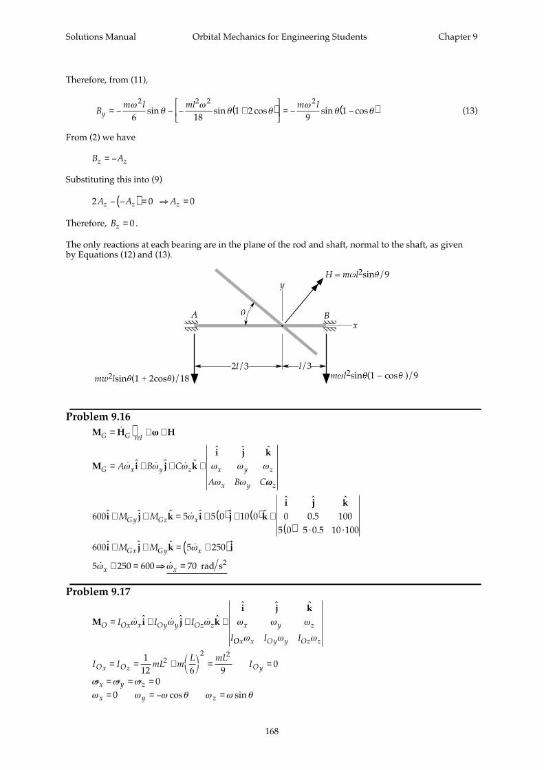
Solutions Manual Orbital Mechanics for Engineering Students Chapter 9
168
Therefore, from (11),
sin sin cos sin cosB
m l ml m ly = − − − +( )
= − −( )ω
θω
θ θω
θ θ2 2 2 2
6 181 2
91 (13)
From (2) we have
B Az z= −
Substituting this into (9)
2 0 0A A Az z z− −( ) = ⇒ =
Therefore, Bz = 0 .
The only reactions at each bearing are in the plane of the rod and shaft, normal to the shaft, as givenby Equations (12) and (13).
Problem 9.16
M H HG G rel
= ) + ×ωω
M i j k
i j k
G x y z x y z
x y
A B C
A B C
= + + +ω ω ω ω ω ω
ω ω
ˆ ˆ ˆˆ ˆ ˆ
ωωz
600 5 5 0 10 0ˆ ˆ ˆ ˆ ˆ ˆˆ ˆ
i j k i j k
i
+ + = + ( ) + ( ) +M MGy Gz xω
jj k
..
0 0 5 1005 0 5 0 5 10 100( ) ⋅ ⋅
600 5 250
5 250 600
ˆ ˆ ˆ ˆ
i j k i+ + = +( )+ =
M MGx Gy x
x
ω
ω ⇒⇒ = ωx 70 rad s2
Problem 9.17
M i j k
i j k
O Ox x Oy y Oz z x y zI I I
I
= + + +ω ω ω ω ω ωˆ ˆ ˆˆ ˆ ˆ
OOx x Oy y Oz zI Iω ω ω
I I mL m
L mLIOx Oz Oy= = +
= =
112 6 9
022 2
« « «ω ω ωx y z= = = 0
ω ω ω θ ω ω θx y z= = − =0 cos sin
2l/3 l/3
A B
y
x
H = m l2sin /9
m l2sin (1 – cos )/9mw2lsin (1 + 2cos )/18
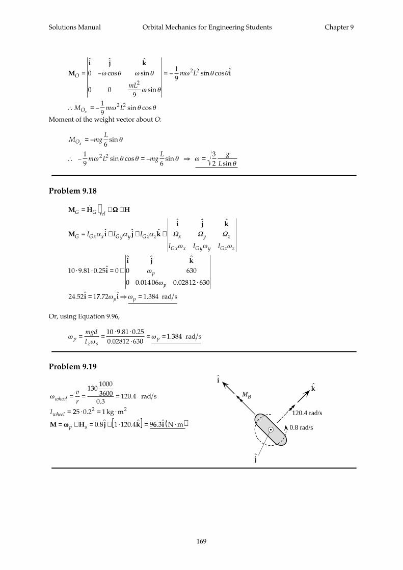
Solutions Manual Orbital Mechanics for Engineering Students Chapter 9
169
M
i j k
O
mL
m L= − = −
ˆ ˆ ˆ
cos sin
sin
si0
0 09
19
2
2 2ω θ ω θ
ω θ
ω nn cos ˆθ θi
∴ = −M m LOx
19
2 2ω θ θsin cos
Moment of the weight vector about O:
M mg
LOx
= −6
sinθ
∴ − = − ⇒ = sin cos sin
sin19 6
32
2 2m L mgL g
Lω θ θ θ ω
θ
Problem 9.18
M H H
M i j k
i
G G rel
G Gx x Gy y Gz zI I I
= ) + ×
= + + +
ΩΩ
α α αˆ ˆ ˆˆ ˆ ˆ
. . ˆ
j k
i
Ω Ω Ωx y z
Gx x Gy y Gz zI I Iω ω ω
10 9 81 0 25 0⋅ ⋅ = +
ˆ ˆ ˆ
. .
. ˆ
i j k
i
0 630
0 0 014 06 0 02812 630
24 52 1
ω
ω
p
p ⋅
= 77 72 1 384. ˆ .ω ωp pi ⇒ = rad s
Or, using Equation 9.96,
ω
ωωp
z sp
mgdI
= =⋅ ⋅
⋅= =
10 9 81 0 250 02812 630
1 384. .
.. rad s
Problem 9.19
ωwheel
wheel
vr
I
= = =
=
13010003600
0 3120 4
.. rad s
225 0 2 1
0 8 1 120 4 9
2⋅ = ⋅
= × = × ⋅[ ] =
.
. ˆ . ˆ
kg m2
M H j kωωp s 66 3. ˆ i N m⋅( )120.4 rad/s
0.8 rad/s
MB
i
j
k
Solutions Manual Orbital Mechanics for Engineering Students Chapter 9
170
Problem 9.20
Irotor
p s
= ⋅ = ⋅
= × = ×
4 0 07 0 0196
2 0 01
2. .
ˆ .
kg m2
M H iωω 996 10000260
41 05⋅ ⋅
= ⋅( )
=
π ˆ . ˆ
k j N m
B Fy
. .
A F
F
F
y = −
=
=
0 04 41 051026 N
Problem 9.21
Irotor
s
= ⋅ = ⋅
= ⋅ =
200 0 25 12 5
15000260
15
2. . kg m2
ωπ
771
65000036002500
0 072 22
.
rad s
rad sωpvr
= = =
=M ωωωωp s× = × −( ) =H i k i0 072 22 12 5 1571 1418. ˆ . ˆ ˆ N ⋅⋅( )m
The moment reaction on the airframe is clockwise, pitching the nose down.
Problem 9.22
M HG p s= ×ωω
ωωp = ( )20i rad s
H k ks = ⋅ ⋅ ⋅ = ⋅( )1
210 0 05 200 2 52. ˆ . ˆ kg m s2
M i k jG = × = − ⋅( )20 2 5 50ˆ . ˆ ˆ N m
0 6 50. ˆ ˆRBj j= −
R R RB A B= − = − =83 33 83 33. . N N
Problem 9.23
lx
xX
= −
= ° ° − ° ° °
= ⋅ − ⋅ ⋅
= −
= −( ) = °−
cos cos sin sin coscos cos sin sin cos
. . . . ..
cos . .
ψ φ φ ψ θ
α
70 50 50 70 250 6428 0 3420 0 7660 0 9397 0 9063
0 4326
0 4326 115 61
k
i
1570.8 rad/s
0.07222 rad/s
j
forwardG
M G C = 12.5 kg - m2
Solutions Manual Orbital Mechanics for Engineering Students Chapter 9
171
Problem 9.24
H I
H
= [ ] =
−
−
=
⋅( )
= ⋅ =
=
ωω
ωω
20 10 010 30 00 0 40
102030
0500
1500
12
12
0 500 1500102030
23 000
J s
JT

Solutions Manual Orbital Mechanics for Engineering Students Chapter 9
172
Solutions Manual Orbital Mechanics for Engineering Students Chapter 10
173
Problem 10.1
ωω
θpsC
A C=
−=
− °=
cos cos.
12002600 1200
66
5 171 rad ss
kg m s2H A p= = ⋅ = ⋅ω 2600 5 171 13 450.
Problem 10.2
ωω
θπ
ωπ
ps
p
CA C
T
=−
=− °
= −
= = =
cos cos.
..
500300 500
610
15 06
2 215 06
0 4173
rad s
s
Problem 10.3
ωω
θω
θω
θ
θθ
θθ θ
θ
ω ωθ
ps s s
p s
CA C
mr
mr mr=
−=
−= −
= −
= −
= + <<( )
∴ = − +
−
cos cos cos
cos
cos
2
2 2
2
2 1 2
2
12
2
12
11
21
20
2 12
Problem 10.4
H A sp= = ⋅ = ⋅ω 1000 2 2000 kg m2
Problem 10.5
H HG rel G) + × =ωω 0
I HG G[ ] + × =αα ωω 0
385 4 0 00 416 7 00 0 52 08
0 010 03
0 02
385 4 0 00 416 7 00 0 52 08
0 010 03
0 02
000
..
.
..
.
..
.
..
.
+ −
×
−
=
αα
385 4 0 00 416 7 00 0 52 08
0 010 03
0 02
3 85412 50
1 042
000
..
.
..
.
..
.
+ −
× −
=
αα
385 4 0 00 416 7 00 0 52 08
0 21880 066 60 009 39
000
..
.
...
+
−
=
αα
385 4 0 00 416 7 00 0 52 08
0 21880 066 60 009 39
000
..
.
...
+
−
=
αα
Solutions Manual Orbital Mechanics for Engineering Students Chapter 10
174
αα = −
−
=
−
−
( )−385 4 0 0
0 416 7 00 0 52 08
0 21880 066 60 009 39
0 000 567 60 00016
0 000180 3
1
2.
..
...
..
. m s
αα = 0 000 6167 2. m s
Problem 10.6
ωω
θω
ps
n
CC A
=−
=− °
= −
=cos
.. . cos
.0 72
0 72 0 3630
1562 12
0
rad s
ω ω θ ψ ω ψ ψ ψ ψ
ω ω θ ψ ω ψ ψ ψ ψ
ω ω ω θ
x p n
y p n
z s p
= + = − ° + ⋅ = −
= − = − ° − ⋅ = −
= + = + −( ) 1 ° = −
sin sin cos . sin sin cos . sin
sin cos cos . sin cos cos . cos
cos . cos
62 12 15 0 16 08
62 12 15 0 16 08
30 62 12 5 30
T A B CR x y z= + +( )= −( ) + −( ) + −( )[ ]= +( ) +[ ]= +( )
=
1212
0 36 16 08 0 36 16 08 0 72 30
12
93 05 648
12
93 05 648
370 5
2 2 2
2 2 2
2 2
ω ω ω
ψ ψ
ψ ψ
. . sin . . cos .
. sin cos
.
. J
Or,
H A sp= = −( ) = − ⋅ω 0 36 62 12 22 36. . . /kg m2
T
HC
C AAR = +−
12
12
2sin θ
..
. ..
sin=−( )
+−
°
12
22 360 72
10 72 0 36
0 3615
22
. .= ⋅ ⋅ +( )1
2694 5 1 0 066 99
. = 370 5 J
Problem 10.7
IG
m l l
m l l
m l l
ml
ml
ml
[ ] =
+ ( )[ ]
+ ( )[ ]( ) + ( )[ ]
=
112
2 0 0
01
123 0
0 01
122 3
512
0 0
056
0
0 01312
2 2
2 2
2 2
2
2
2
H I0
2
2
2
0
0
0
20
20
20
512
0 0
056
0
0 01312
1 50 80 6
0 6250 6667
0 65 = [ ] =
=
G
ml
ml
ml
ml
ml
mlωω
.
.
.
..
.
ω
ω
ω
ω
ω
ω
H ml02
01 121= . ω

Solutions Manual Orbital Mechanics for Engineering Students Chapter 10
175
T
ml
ml
ml
ml0 0 0 0 0
20
20
20
20
212
12
1 5 0 8 0 60 625
0 66670 65
0 9305= ⋅ =
=ωω H . . ..
..
.ω ω ω
ω
ω
ω
ω
(a)
T C ml ml
T T
ml ml
= = =
=
=
= =
12
12
1312
0 5417
0 5417 0 9305
1 718 1 311
2 2 2 2 2
02 2 2
02
0 0
ω ω ω
ω ω
ω ω ω
.
. .
. .
(b)
H C ml
H H
ml ml
= =
=
=
=
ω ω
ω ω
ω ω
1312
1312
1 121
1 035
2
0
2 20
0
.
.
Problem 10.8
H initial = ⋅ = ⋅1000 6 6000 kg m s2
Tinitial = ⋅ ⋅ = ⋅
12
1000 6 18 0002 kg m s2 2
H final final= 5000ω
H Hfinal initial=
5000 6000ω final =
ω final = 1 2. rad s
T final final= ⋅ ⋅ = ⋅ ⋅ = ⋅
12
500012
5000 1 2 36002 2ω . kg m s2 2
∆T T Tfinal initial= − = − = −3600 18 000 14 400 J
Problem 10.9
HG0
0 1522 0 03975 0 0120 03975 0 07177 0 040570 012 0 04057 0 1569
1000
1 5220 3975
0 1200 =
−
−
= −
⋅( ). . .. . .. . .
..
.kg m s2
HG G0 0 1 5776= = ⋅H . kg m s2
T G0 0 012
12
1 522 0 3975 0 12001000
7 610= ⋅ = −
=H ω . . . . J
I max . = ⋅ ( )0 1747 kg m from Example 10.112
H IG f f f= =max .ω ω0 1747
H HG f G= 0
0 1747 1 578. .ω f =
ω f = 9 03. rad s
Solutions Manual Orbital Mechanics for Engineering Students Chapter 10
176
T If f= ⋅ = ⋅ ⋅ =
12
12
0 1747 9 03 7 1232 2max . . .ω J
∆T T Tf= − = − = −0 7 123 7 610 0 4867. . . J
Problem 10.10
C C C C
C
C C
rr
pr
relp
rr
pr
relp
r r p relp
relp
p r
r
ω ω ω ω ω ω
ω ωω ω
ω
2 2 2 1 1 1
2 11 2
2 3500 1 0 5500 1000
3 167
( ) ( ) ( ) ( ) ( ) ( )
( ) ( )( ) ( )
( )
+ +( ) = + +( )
= +−( )
+
= +−( )
+=
.. rad s
Problem 10.11
ωω
θπω
π
ps
p
CA C
t
=−
=− °
=
= = =
cos.
cos.
..
10005000 1000
0 120
0 0266
0 0266118 1
rad s
s
Problem 10.12
cos
tan
γφ
=
+
A
A C2 2 22
A
mr l C mr= +( ) = ⋅ +( ) = ⋅ = = ⋅ = ⋅
123
50012
3 0 5 2 197 912
12
500 0 5 62 52 2 2 2 2 2. . . . kg m kg m2 2
φ
γ=
−
= °
−
= °− −2 2
197 95
197 9
62 530 971
22
21
22
2tancos
tan
.cos
.
..
AA
C
Problem 10.13
Npd I= −( )ω ω2 1
ω ω2 1= +
NpdI
ω π2 0 01 2
30 15 1 52000
0 4003 0 0637= ⋅ +⋅ ⋅
= =..
. . rad s rev s
Problem 10.14
H i j k
i
G x y zA B C0 0 0 0
2000 0 1
= + +
= ⋅
ω ω ωˆ ˆ ˆ
. ˆ ++ ⋅ + ⋅
= +
4000 0 3 6000 0 5
200 1200
. ˆ . ˆ
ˆ ˆj k
i jj k+ 3000 ˆ
H H H
i j k i
G G G= +
= + + + −
0
200 1200 3000 50 1
∆
ˆ ˆ ˆ ˆ 000 300
250 1100 3300
ˆ ˆ
ˆ ˆ ˆj k
i j k
+( )= + +
Solutions Manual Orbital Mechanics for Engineering Students Chapter 10
177
A B Cx y zω ω ωˆ ˆ ˆ ˆ ˆ ˆi j k i j k+ + = + +250 1100 3300
ω x A
= = =250 250
20000 125. rad s
ω y B
= = =1100 1100
40000 275. rad s
ω z C
= = =3300 3300
60000 55. rad s
ω ω ω ω= + + =x y z
2 2 2 0 6275. rad s
Problem 10.15
A mr ml
C mr
= + = ⋅ + ⋅ = ⋅
= = ⋅ = ⋅
14
112
14
300 1 51
12300 1 5 225
12
12
300 1 5 337 5
2 2 2 2
2 2
. .
. .
kg m
kg m
2
2
H k k kG C
1 1 337 5 1260
35 34= = ⋅ ⋅
= ⋅ωπˆ . ˆ . ˆ kg m2(( )
H HG G M2 1
= + II
H k jG M2
35 34= + −( ). ˆ ˆI
HG M M2
35 34 12492 2 2= + = +. I I
H AG p2
= ω
1249 225 0 1 2 141 42+ = ⋅ ⋅( ) =IM . .π
I
I
M
M
2 18740136 9=
= ⋅ ⋅. N m s
Problem 10.16
K
C
mR= + = +
⋅ ⋅=1
21
300
2 3 1 523 222 2.
.
(a)
l R K
tK
ff
f
f
f
=−
+= ⋅
−+
=
−
+=
−+
=
ω ω
ω ω
ω
ω ω
ω ω
0
0
02
0
02
1 5 23 225 15 1
5 902
23 22
5
5 15 1
0 7869
. . .
..
m
= s
(b)
l R K
tK
ff
f
f
f
=−
+= ⋅
−+
=
−
+=
−+
=
ω ω
ω ω
ω
ω ω
ω ω
0
0
02
0
02
1 5 23 225 05 0
7 228
23 22
5
5 05 0
0 9636
. . .
..
m
= s
Solutions Manual Orbital Mechanics for Engineering Students Chapter 10
178
Problem 10.17
T A C A Cx y z0
2 2 2 20
212
12
12
12
= +( ) + = +ω ω ω ωΩ
ω
ωθp
sCA C
=−
=− °
= −cos cos
.60
30 60215
4 141 rad s
ω ω θ0
3060
4 141 15 2= = −( ) ° = −AC p cos . cos rad s
Ω = = − ° = −ω θp sin . sin .4 141 15 1 072 rad s
∴ = ⋅ −( ) + ⋅ −( ) =T0
2 212
30 1 07212
60 2 137 2. . J
(a)
H A p0 30 4 141 124 2= = ⋅ = ⋅ω . . kg m s2
H Hf = 0
60 124 2 2 071ω ωf f= ⇒ =. . rad s
(b)
T Cf f= = ⋅ ⋅ =
12
12
60 2 071 128 62 2ω . . J
∆T T Tf= − = − = −0 128 6 137 2 8 616. . . J
(c)
l R
C
mRf = + = ⋅ +
⋅ ⋅=1
21 1
60
2 7 12 2992 2 . m
Problem 10.18
H IG G
s s
A
A
C
n nA
C = [ ] =
−
=
−
ωω
0 00 00 0
0 0
ω ω
M H
i j k
iG G
s
sn
nA C
C n= × =
−
= −ΩΩ 00
ˆ ˆ ˆˆ0
0 ω
ω
ωπ
ππ
s
n
C
= ⋅ =
=+
⋅= ×
⋅
−
1260
0 1047
22
365 2624 3600
7 292 10
550
5
.
. .
rad /s
rad /s
= kg m2
∴ = − ⋅ ⋅ × = − ⋅−MGx 550 0 1047 7 292 10 0 004 25. . . N m
Problem 10.19 ωω0 and ωω f are the initial and final angular velocities of the spacecraft. ω is the
angular velocity of the flywheel relative to the vehicle.
H H H HG
vGv
Gv w
f( ) ( ) ( ) ( )+[ ] = +[ ]0
A A C I I Ix y z x x y y zω ω ω ω ω ω0 0 0 0 0 0ˆ ˆ ˆ ˆ ˆi j k i j+ +( ) + + + zz
x y z x x y yA A C I I
ˆ
ˆ ˆ ˆ ˆ ˆ
k
i j k i
( )= + +( ) + +( ) +ω ω ω ω ω ω jj k+
Iz zω ˆ
Solutions Manual Orbital Mechanics for Engineering Students Chapter 10
179
A I A Iz z z z z z+( ) = +( ) ⇒ = =ω ω ω ω0 0 0
A I A Iy y y y y y+( ) = +( ) ⇒ = =ω ω ω ω0 0 0 05 . rad s
A I I A I
AIx x x x x
xx x+( ) + = +( ) ⇒ = +
−( )ω ω ω ω ω ω0 01
∴ = +
−( ) =ω 1
100020
0 1 0 003 4 947. . . rad s
Problem 10.20
Given: I I I3 2 1> > .
Figure 10.29, Stable region I: I I Iroll yaw pitch> > :
I1 axis in pitch direction (normal to orbital plane)
I2 axis in yaw direction (radial)
I3 axis in roll direction (local horizon)
Figure 10.29, Stable region II (preferred): I I Ipitch roll yaw> > :
I1 axis in yaw direction (radial)
I2 axis in roll direction (local horizon)
I3 axis in pitch direction (normal to orbital plane)
Solutions Manual Orbital Mechanics for Engineering Students Chapter 10
180
Solutions Manual Orbital Mechanics for Engineering Students Chapter 11
181
Problem 11.1
m m m m
mmp pout pin pout
poutpout
= + = + =4
54
Outbound leg:
∆v I gm m m
m m m m
m m
m m m
m m
m m
sp oe p PL
e p pout PL
e pout
e pout pout
e pout
e pout
=+ +
+ − +
= ⋅ ⋅+ +
+ − +
= ⋅ ⋅+ +
+ +
ln
. ln
. ln
4220 430 9 81
54
3500
54
3500
430 9 81
54
3500
14
3500
m m
m m
e pout
e pout
+ +
+ +=
54
3500
14
35002 719.
0 5702 1 719 6018. .m mpout e− = (1)
Return from GEO tp LEO:
∆v I g
m m
msp oe pout
e=
+ +
ln
14
3500
4220 430 9 81
14= ⋅ ⋅
+
. ln
m m
m
e pout
e
m m
m
e pout
e
+=
14 2 719.
m mpout e= 6 876. (2)
Substitute (2) into(1):
0 5702 6 876 1 719 60182733
. . .m m
me e
e
( ) − =
= kg
Problem 11.2
First stage:
c I gsp o= = ⋅ =235 9 81 2943. m s
v c
mm
m m g
mbof
f o
e=
−
−( )=
−
−( ) ⋅= − =ln
«ln
.
.. . .
..0 0
2943249 5170 1
249 5 170 1 9 8110 61
1127 73 38 1054 m s
h
cm
m
mm m m
m m
mgbo
e
ff f
f
eo=
+ −
−
−
«
ln«0
00
212
.ln
.
.. . .
. ..
.=
⋅ + −
−
−
294310 61
170 1249 5
170 1 249 5 170 112
249 5 170 110 61
9 812
Solutions Manual Orbital Mechanics for Engineering Students Chapter 11
182
.
= −
=
3947 274 43673 m
After 3 second staging delay:
v v g tbo s= − = − ⋅ =∆ 1054 9 81 3 1024. m s
h h v t g tbo bo s s= + − = + ⋅ − ⋅ ⋅ = + =∆ ∆
12
3673 1054 312
9 81 3 3673 3117 67902 2 m.
Second stage:
v
h0
0
10246790
=
=
m s m
c I gsp o= = ⋅ =235 9 81 2305. m s
v v cmm
m m g
mbof
f o
e= +
−
−( )
= +
−
−( ) ⋅
= + −
=
00 0
1024 2305113 458 97
113 4 58 97 9 814 0573
1024 1508 131 72400
ln«
ln.
.. . .
. . m s
h h v
m m
mc
m
m
mm m m
m m
mgbo
f
e e
ff f
f
eo= +
−
+
+ −
−
−
0 0
0
00
02
12« «
ln«
. .. .
ln..
. . .. .
..= +
−
+
⋅ + −
−
−
⋅6790 1024
113 4 59 974 053
23054 053
59 97113 4
58 97 113 4 58 9712
113 4 58 974 063
9 812
.= + + −6790 13760 9028 884 7
= 28 690 m
Coast to apogee:
v
h0
0
240028 690
=
=
m s m
0
24009 81
244 700= − ⇒ = = =v gt t
vgmax max
.. s
h h v t gtmax max max . . .= + − = + ⋅ − ⋅ ⋅ =0 0
2 212
28 690 2400 244 712
9 81 244 7 322 300 m
Problem 11.3
v R057 292 10 6378 28 0 4107= = ( ) ⋅ ⋅ ° =−ω φearth earth km scos . cos .
∆v = + − =
398 6006678
2 0 4107 9 315. . km s
v vbo = =∆ 9 315. km s
v v vbo bo bo= +1 2
v I gm
mI g
m
mbo sp of
sp of
=
+
1
01
12
02
2
ln ln
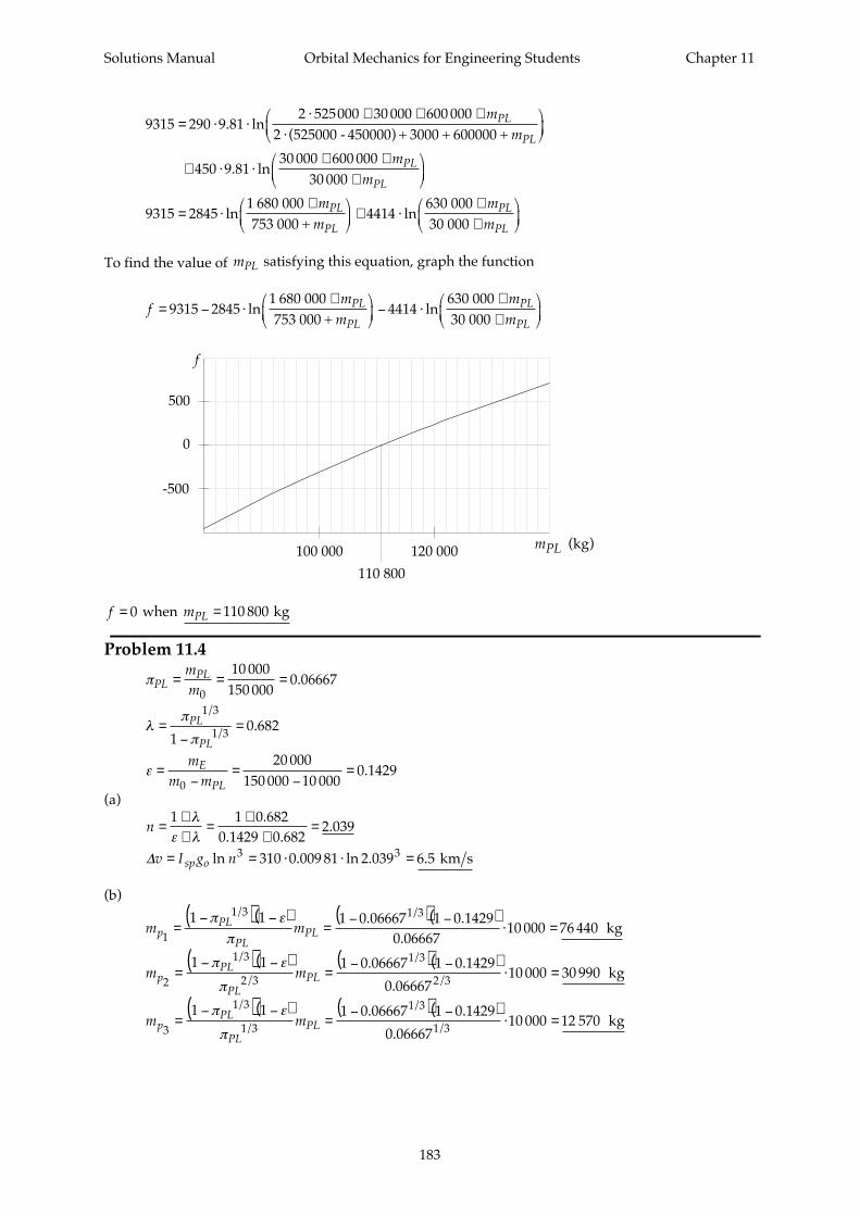
Solutions Manual Orbital Mechanics for Engineering Students Chapter 11
183
9315 290 9 812 525000 30 000 600 000
450 9 8130 000 600 000
30 000
= ⋅ ⋅⋅ + + +
⋅
+ ⋅ ⋅+ +
+
. ln
. ln
mm
mm
PL
PL
PL
PL
2 (525000 - 450000) + 3000 + 600000 +
9315 2845
1 680 0007
4414630 00030 000
= ⋅+
+ ⋅
+
+
ln ln
mm
mm
PL
PL
PL
PL53 000 +
To find the value of mPL satisfying this equation, graph the function
f
mm
mm
PL
PL
PL
PL= − ⋅
+
− ⋅
+
+
9315 2845
1 680 0007
4414630 00030 000
ln ln53 000 +
f = 0 when mPL = 110 800 kg
Problem 11.4
π
λπ
π
ε
PLPL
PL
PL
E
PL
mm
mm m
= = =
=−
=
=−
=−
=
01 3
1 3
0
10 000150 000
0 06667
10 682
20 000150 000 10 000
0 1429
.
.
.
/
/
(a)
n
v I g nsp o
=++
=+
+=
= = ⋅ ⋅ =
1 1 0 6820 1429 0 682
2 039
310 0 009 81 2 039 6 53 3
λε λ
.. .
.
ln . ln . .∆ km s
(b)
m mp
PL
PLPL1
1 3 1 31 1 1 0 06667 1 0 14290 06667
10 000 76 440=−( ) −( )
=−( ) −( )
⋅ =π ε
π
/ /. ..
kg
m mp
PL
PLPL2
1 3
2 3
1 3
2 31 1 1 0 06667 1 0 1429
0 0666710 000 30 990=
−( ) −( )=
−( ) −( )⋅ =
π ε
π
/
/
/
/. .
. kg
m mp
PL
PLPL3
1 3
1 3
1 3
1 31 1 1 0 06667 1 0 1429
0 0666710 000 12 570=
−( ) −( )=
−( ) −( )⋅ =
π ε
π
/
/
/
/. .
. kg
-500
0
500
100 000 120 000
110 800
mPL (kg)
f
Solutions Manual Orbital Mechanics for Engineering Students Chapter 11
184
(c)
m m
m m
m m
EPL
PLPL
EPL
PLPL
EPL
PLPL
1
1 3 1 3
2
1 3
2 3
1 3
2 3
3
1 3
1 3
1 1 0 06667 0 14290 06667
10 000 12740
1 1 0 06667 0 1429
0 0666710 000 5166
1 1 0
=−( )
=−( ) ⋅
=
=−( )
=−( ) ⋅
=
=−( )
=−
π ε
π
π ε
π
π ε
π
/ /
/
/
/
/
/
/
. ..
. .
.
kg
kg
.. .
.
/
/06667 0 1429
0 0666710 000 2095
1 3
1 3
( ) ⋅= kg
(d)
m m m m
m m m m
m m m m
E p PL
E p
E p
03 3 3
02 2 2 03
01 1 1 02
2095 12 570 10 000 24 660
5166 30 990 24 660 6
12740 76 440 6 1
= + + = + + =
= + + = + + =
= + + = + + =
kg
0 820 kg
0 820 50 000 kg
Problem 11.5
c I g
c I g
sp o
sp o
1 1
2 2
300 0 009 81 2 943
235 0 009 81 2 305
= = ⋅ =
= = ⋅ =
. .
. .
km s
km s
ε
ε1
2
0 20 3
=
=
..
vbo = 6 2. km s
v c
cc
ccc
cccbo i
i
i ii=
−
=
−
+
−
=∑ ln ln ln
ηε η
ηε η
ηε η
1 1 1
1
2
11
1 12
2
2 2
6 2 2 943
2 943 12 943 0 2
2 3052 305 12 305 0 3
. . ln.. .
. ln.. .
=−
⋅
+
−⋅
ηη
ηη
6 2 2 943
2 943 10 5886
2 3052 305 10 6915
. . ln..
. ln..
=−
+
−
ηη
ηη
To find η , graph the function
f =
−
+
−
−2 943
2 943 10 5886
2 3052 305 10 6915
6 2. ln..
. ln..
.ηη
ηη
As shown below, f = 0 when η = 1 726. .
n
cc11
1 1
1 2 943 1 726 12 943 0 2 1 726
4 016=−
=⋅ −⋅ ⋅
=ηε η
. .. . .
.
n
cc22
2 2
1 2 305 1 726 12 305 0 3 1 726
2 496=−
=⋅ −⋅ ⋅
=ηε η
. .. . .
.
m
nn
mPL22
2 2
11
2 496 11 0 3 2 496
10 59 53=−
−=
−− ⋅
⋅ =ε
.. .
. kg
m
nn
m mPL11
1 12
11
4 016 11 0 2 4 016
59 53 10 1065=−
−+( ) =
−− ⋅
+( ) =ε
.. .
. kg
M m m= + = + =1 2 1065 59 53 1124. kg
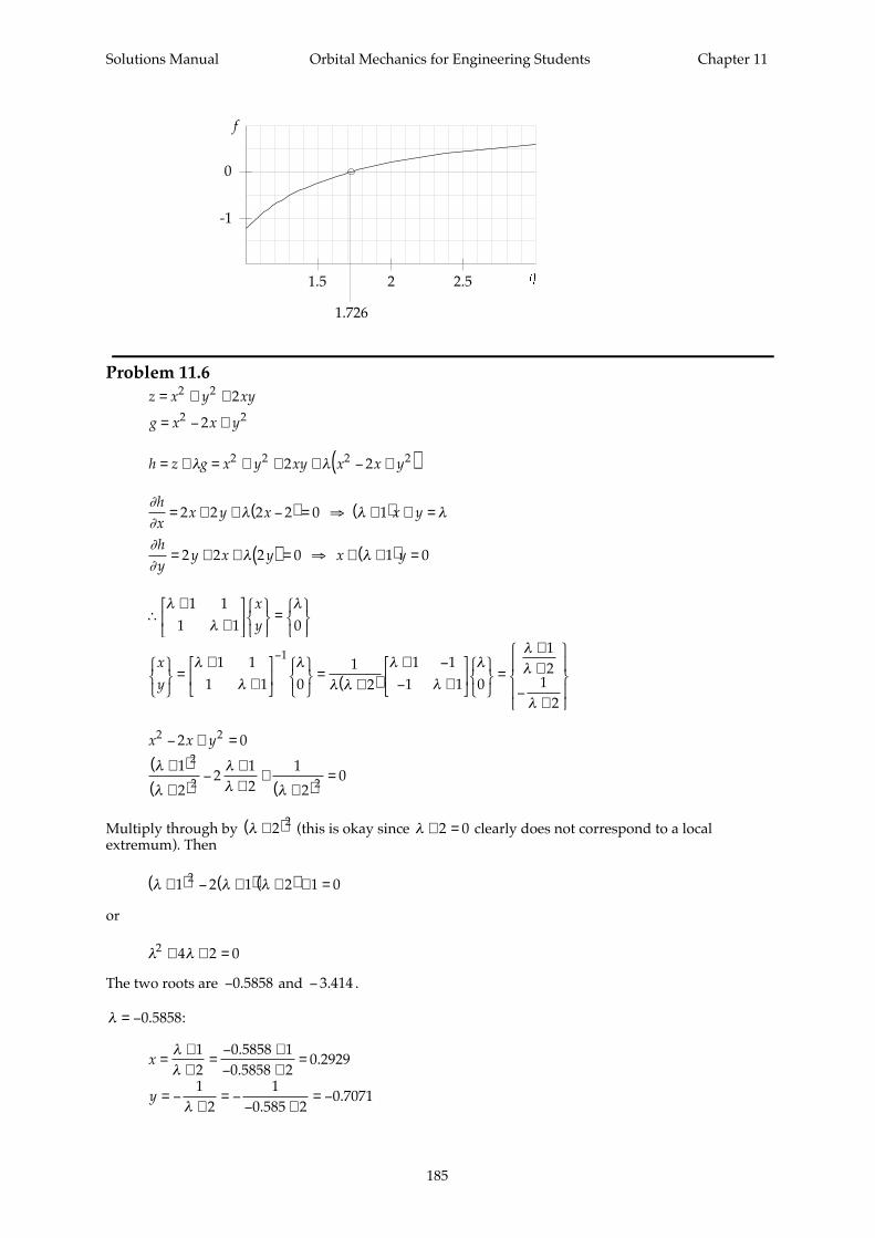
Solutions Manual Orbital Mechanics for Engineering Students Chapter 11
185
Problem 11.6
z x y xy
g x x y
= + +
= − +
2 2
2 2
2
2
h z g x y xy x x y= + = + + + − +( )λ λ2 2 2 22 2
∂
∂λ λ λ
hx
x y x x y= + + −( ) = ⇒ +( ) + =2 2 2 2 0 1
∂
∂λ λ
hy
y x y x y= + + ( ) = ⇒ + +( ) =2 2 2 0 1 0
∴
+
+
=
λ
λ
λ1 11 1 0
x
y
x
y
=+
+
=+( )
+ −
− +
=
++
−+
−λ
λ
λ
λ λ
λ
λ
λλλ
λ
1 11 1 0
12
1 11 1 0
12
12
1
x x y2 22 0− + =
λ
λ
λλ λ
+( )
+( )−
++
++( )
=1
22
12
1
20
2
2 2
Multiply through by λ +( )2 2 (this is okay since λ + =2 0 clearly does not correspond to a localextremum). Then
λ λ λ+( ) − +( ) +( ) + =1 2 1 2 1 02
or
λ λ2 4 2 0+ + =
The two roots are −0 5858. and − 3 414. .
λ = −0 5858. :
x =
++
=− +− +
=λλ
12
0 5858 10 5858 2
0 2929..
.
y = −
+= −
− += −
12
10 585 2
0 7071λ .
.
1.5 2 2.5
-1
0
1.726
f
Solutions Manual Orbital Mechanics for Engineering Students Chapter 11
186
z x y xy12 2 2 22 0 2929 0 7071 2 0 2929 0 7071 0 1716= + + = + −( ) + ⋅ −( ) =. . . . .
λ = −3 414. :
x =
++
=− +− +
=λλ
12
3 414 13 414 2
1 707..
.
y = −
+= −
− +=
12
13 414 2
0 7071λ .
.
z x y xy22 2 2 22 1 707 0 7071 2 1 707 0 7071 5 828= + + = + + ⋅ ⋅ =. . . . .
Note that
d h
z
x
g
xdx
zx y
gx y
dxdyz
y
g
ydy2
2
2
2
22
2 2 2
2
2
222= +
+ +
+ +
∂
∂λ∂
∂
∂∂ ∂
λ∂∂ ∂
∂
∂λ∂
∂
d h dx dxdy dy2 2 22 2 2 2 0 2 2= + ⋅( ) + + ⋅( ) + + ⋅( )λ λ λ
d h dx dy dxdy2 2 22 1 4= +( ) +( ) +λ
For λ = −0 5858. ,
d h dx dy dxdy dx dy dxdy
dx dy dxdy
2 2 2 2 2
2 2
2 1 4 2 0 5858 1 4
0 8284 4
= +( ) +( ) + = − +( ) +( ) +
= +( ) +
λ .
.
Since d h2 0> , z z1 = min .
For λ = −3 414. ,
d h dx dy dxdy dx dy dxdy
dx dy dxdy
2 2 2 2 2
2 2
2 1 4 2 3 414 1 4
4 828 4
= +( ) +( ) + = − +( ) +( ) +
= − +( ) +
λ .
.
Since d h2 0< , z z2 = max .