Arnold, S. (2010) Environmental Decision Making and Behaviours: How to People Choose how to Travel to Work? Working Paper. Department of Economics, University of Bath, Bath, UK. (Unpublished)

Link to official URL (if available): http://www.bath.ac.uk/economics/research/workingpapers.html

Opus: University of Bath Online Publication Store

http://opus.bath.ac.uk/

This version is made available in accordance with publisher policies. Please cite only the published version using the reference above.

See http://opus.bath.ac.uk/ for usage policies.

Please scroll down to view the document.

1

Environmental Decision Making and Behaviours: How to People Choose how to

Travel to Work?

Steven Arnold

No. 07/10

BATH ECONOMICS RESEARCH PAPERS

Department of Economics

2

Environmental decision making and

behaviours: How do people choose how

to travel to work?

Steve Arnold Department of Economics, University of Bath

1.

Abstract: The daily commute is an important element of transport and travel

behaviour in the UK, and as such is relevant to discussions about the environment

and sustainability, as well as social well-being. Economic research on the matter

focuses on cost and structural factors, with preferences being given, whilst the

psychological literature looks at how preferences are formed from attitudes and

values, but tends to underplay the role of structural variables. This paper develops a

simple structure of how attitudes, values and behaviours are linked, and tests them

with multinomial and ordered regressions using data from Defra’s 2007 Survey of

Attitudes and Behaviours in Relation to the Environment. The results found that

attitudes towards cars and driving were a significant factor in transport choices, but

environmental beliefs were only mildly significant, and only for some travel

choices. Structural variables, here proxied by distance to work, were influential in

most travel choices, as was age. Stated environmental behaviours however, were

almost entirely insignificant. The results were robust, and suggest that policies

aimed at structural or attitudinal change would be more effective than policies

aimed at changing people’s environmental values.

Key Words: Transport, Commute, Environment, Values, Attitudes, Decision-making

JEL Codes: R41, Q50

1 Claverton Down, Bath, BA2 7AY, UK. The author can be contacted at s.arnold@bath.ac.uk

The author would like to thank Prof. Anil Markandya and Mr. Tim Taylor for the helpful comments and suggestions

on this paper. Any mistakes that remain are my own.

3

INTRODUCTION

Understanding the factors that lie behind people’s daily commuting decisions is important for

both transport and environmental policy, but too often, the psychological, sociological and

economic aspects of such research have been kept apart. Previously, there has been a separation

of investigations, with some academic research looking at the economic and structural factors

which influence people's choices, and other research - led by psychologists and sociologists -

looking at how values and attitudes lead to choices being made. Very little has been done to

combine the two, particularly in the realm of transport economics. This is surprising, since it

seems likely that both aspects combine in many people's process-making.

This paper will look at how individuals' environmental attitudes and values shape their choice of

method by which they travel to work. That is, it will ask whether people are affected by their

concern or understanding of environmental issues to the extent that they will travel by methods

perceived to be more environmentally aware or, on the other hand, do financial and structural

concerns override most people's environmental values?

LITERATURE REVIEW

Economic Literature

A large number of the transport economics papers which look at decision making are largely

based on McFadden's 1974 paper, which took the proposed development of a public transport

system in San Francisco as its basis. A binary decision was modelled where people were

assumed to have the choice of travelling by car or by the new public transport system. Costs of

both private and public transport were estimated, including the costs of time spent waiting and

travelling. A “pure auto-mode” preference effect was also calculated which found that over half

the population would travel by car even if costs and times for public transport were zero.

However, no variables were tested that looked at environmental beliefs or values, other than

possibly “People drive cars that are too big” and “Buses smell of fumes”, both of which were

insignificant at the 5% level. The paper discusses the variables that correspond to attitudes in

taste and behaviour (such as becoming angry in traffic jams) and reasons that it is better from a

policy analysis view to bypass researching people’s attitudes and go straight to researching the

policies that may have shaped these.

One issue which McFadden treated as exogenous in his study was residential location. He

recognised the sample selection issues concerning how people made choices based around where

they live, found that people think living near public transport is a key decision in choosing that

travel method. Other studies have looked at the relationship between housing location choice and

travel choice in more depth, such as Cervero and Radisch (1996), Kitamura et al (1997), Cervero

(2002), Bagley and Mokhtarian (2002), Schwanen and Mokhtarian (2005), and Feldman and

Simmonds (2007). A range of hypothesis have been raised and tested to study how people may

choose a neighbourhood on the basis of the travel commitments it would involve, or how people

4

choose travel methods based on the neighbourhood characteristics, or how these may interact

with each other. The dynamic inter-relationships of two importance choices – work and home

location – mean that such studies are not completely pertinent here. However, it is crucial to note

that environmental attitudes and values can play a role in such large decisions.

When considering values and behaviours against more structural variables such as location,

Kitamura et al (1997) found that attitudes have a stronger or more direct association with travel

than local land use characteristics. That is, factors such as local housing density and public

transport accessibility were found to be less influential than attitudes such as “driving allows me

more freedom” and “too many people drive alone”.

Similarly, Bagley and Mokhtarian (2002) find that the attitudinal and lifestyle variables, such as

a tendency to accept pro-environmental statements, have a stronger effect on travel choice than

the location. Their methodology was based on the structural equations modelling (SEM)

approach, and the same dataset as Kitamura et al (1997) from San Francisco. They find that pro-

environmental beliefs are linked to pro-high-density and pro-transit attitudes, and lead to an

increase in transit miles and commute distance, but no significant relationship with miles cycled.

Overall, Bagley and Mokhtarian (2002) find that residential location has very little impact on

travel behaviour, which suggests that personal variables, such as beliefs, have a stronger impact

than structural variables such as location. This may be because personal variables influence the

choice of location, but the SEM approach attempts to capture such interrelations. The authors

note that both attitudes and behaviours change over time, and people adapt to the situations they

are in, but overall the study “found no impact of residential location on attitudes” (Bagley and

Mokhtarian, 2002:295, emphasis theirs). Dynamic interrelationships were outside the scope of

their study, but it is an interesting side-note to reflect upon how changeable variables can be.

One study that looks in particular at the travel decisions to work across the UK was carried out

by Parkin et al (2008), who studied the factors that lie behind cycling to work. Although it would

seem likely that this would be, at least in part, related to environmental attitudes, the study does

not look into this aspect. Rather, it examines physical and infrastructure variables, such as road

condition, hilliness and the presence of cycle paths. Hilliness is found to be a key variable, which

suggests that structural factors are key to people’s decision making and behaviour. Similarly,

Black et al (2001) look at factors which influence people’s decision to walk to school. Again,

structural factors are key, in this case, difficulty parking at school and square of distance among

the significant results. Subsequent research was able to divide the respondents into three groups

but the Environmental Awareness group was the least influential2.

Overall, the literature on transport decisions makes little reference to environmental values as an

explanatory variable. Black et al (2001) use a range of questions on environmental and personal

attitudes to travel, and find some significantly affect people’s decisions to walk to school.

However, the wider range of literature suggests that there are complex interactions between the

variables, and that the decisions are made through a process over time. The next section of this

paper will therefore look at the wider, less economic-based literature into travel decision making

and environmental beliefs.

2 The other groups were Individual Responsibility and Awareness, and Car-Centredness.

5

Psychological Literature

There is a field of psychology that looks at how environmental behaviour is related to both

attitudes and values (see Davies et al, 2002 and Schultz et al, 1995 for summaries). This

literature largely ignores financial/economic incentives to behaviour, and instead assumes that

what drives an action or behaviour are the underlying values and perspectives on the world. Of

particular interest is how values and attitudes can be ‘layered’, with broad values (e.g. about the

environment) not entirely aligned with more precise attitudes, for example about recycling.

Eagly and Kulesa (1997) define attitudes as the “psychological tendency that is expressed by

evaluating a particular entity with some degree of favour or disfavour.” Overarching attitudes are

known as values. Based on Katz (1960), they discuss how people can change their attitudes (or

have their attitudes changed) by changing values. These definitions are subject to a degree of

discussion but in general, it is accepted that people have different types of attitude or values

which can influence each other and influence behaviour in different ways.

Looking first at values, there is a body of literature than examines how environmental values are

linked to transport decisions. There is mixed evidence for how transport preferences are

associated with concern for the environment, pro-social orientations and pro-individual values.

Joireman et al (2004) summarise the findings from Van Vugt et al (1995 and 1996), Van Lange

et al (1998) and Joireman et al (1997); although these come from a broad ‘family’ of research

using the social dilemma model, the results are not conclusive. Joireman et al (2004) then test

whether travel decisions are based on people’s temporal concerns, that is, whether they are

consider future consequences or not, and they find that the relationship between people’s

perceptions of the negative environmental impact of cars and preference for public transport was

only significant when there was a high consideration of future impact. This suggests that the

interrelationships between values and preferences can be complex and affect each other.

Other studies have looked at what may limit the relationship between values, beliefs and

behaviour. Derksen and Gartrell (1993) found that environmental attitudes only affect behaviour

in communities with easy access to recycling. Similarly, Diekmann and Preisendörfer (2003) test

the hypothesis that environmental concern influences environmental behaviour primarily in low-

cost or low-hassle situations, but found none was significantly correlated to stated environmental

concern. The authors suggest that this is because such travel behaviours are “high-cost” and so

leave little room for people’s concern.

Grob (1995) developed and tested a model of the relationships between environmental attitudes

and pro-environmental behaviour, which is summarised in Figure 1. Figure 1: Grob’s Model of Environmental Behaviour. Source: Grob (1995)

Personal

Philosophical

Values

Environmental

Awareness

Emotions

Perceived

Control

Environmental

Behaviour

6

In general, the accuracy of this research is hard to estimate since the key variable measured does

not consider differences in various types of environmental behaviour. Also, Grob recognises that

the model only represents individual level research, and reflects that "it would be worthwhile to

include other categories on influence (i.e. socio-economic, geographical, and cultural location) to

gain a more comprehensive pattern of the extent to which environmental behaviours are due to

physical, individual, historical and cultural influences" (p.218). However, it seems robust enough

to show that the model shown in Figure 1 would be a useful mental picture of the sorts of value-

attitude-behaviour relationships tested in this paper.

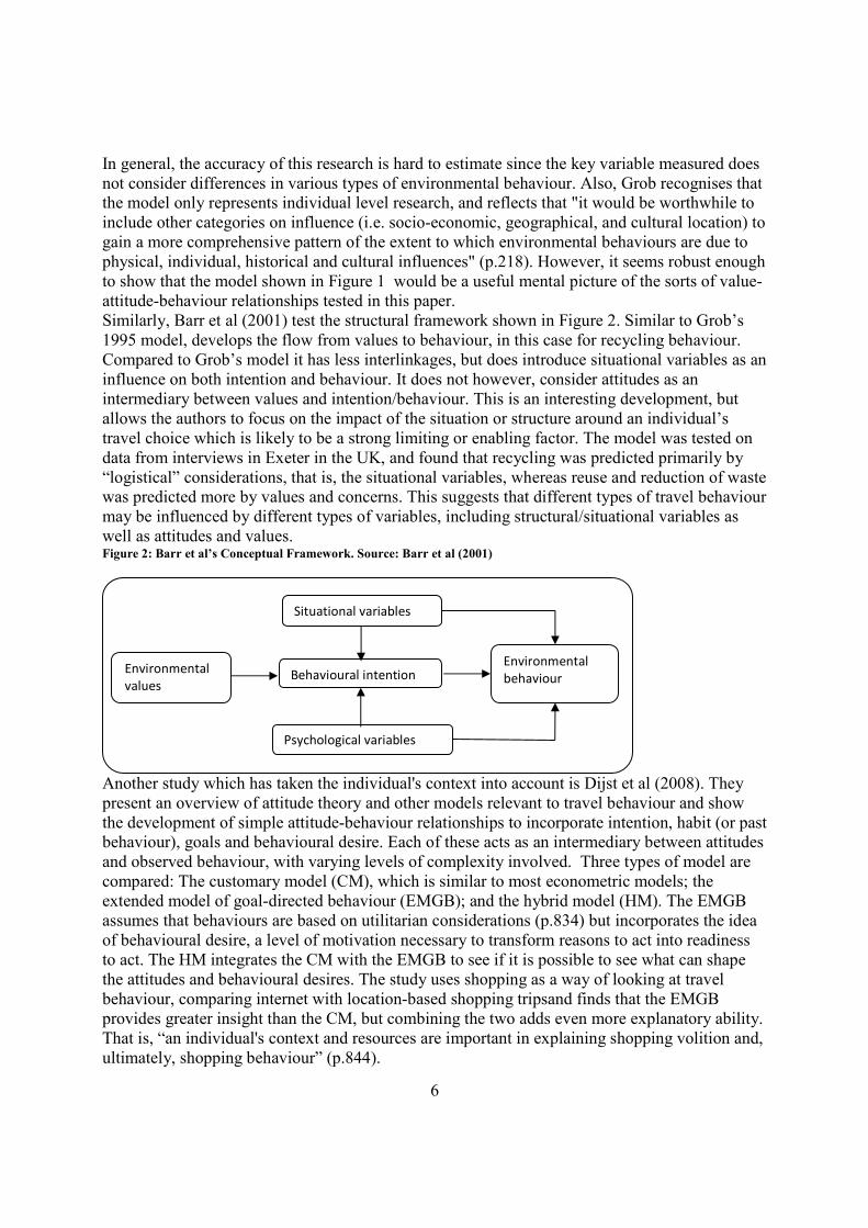
Similarly, Barr et al (2001) test the structural framework shown in Figure 2. Similar to Grob’s

1995 model, develops the flow from values to behaviour, in this case for recycling behaviour.

Compared to Grob’s model it has less interlinkages, but does introduce situational variables as an

influence on both intention and behaviour. It does not however, consider attitudes as an

intermediary between values and intention/behaviour. This is an interesting development, but

allows the authors to focus on the impact of the situation or structure around an individual’s

travel choice which is likely to be a strong limiting or enabling factor. The model was tested on

data from interviews in Exeter in the UK, and found that recycling was predicted primarily by

“logistical” considerations, that is, the situational variables, whereas reuse and reduction of waste

was predicted more by values and concerns. This suggests that different types of travel behaviour

may be influenced by different types of variables, including structural/situational variables as

well as attitudes and values. Figure 2: Barr et al’s Conceptual Framework. Source: Barr et al (2001)

Another study which has taken the individual's context into account is Dijst et al (2008). They

present an overview of attitude theory and other models relevant to travel behaviour and show

the development of simple attitude-behaviour relationships to incorporate intention, habit (or past

behaviour), goals and behavioural desire. Each of these acts as an intermediary between attitudes

and observed behaviour, with varying levels of complexity involved. Three types of model are

compared: The customary model (CM), which is similar to most econometric models; the

extended model of goal-directed behaviour (EMGB); and the hybrid model (HM). The EMGB

assumes that behaviours are based on utilitarian considerations (p.834) but incorporates the idea

of behavioural desire, a level of motivation necessary to transform reasons to act into readiness

to act. The HM integrates the CM with the EMGB to see if it is possible to see what can shape

the attitudes and behavioural desires. The study uses shopping as a way of looking at travel

behaviour, comparing internet with location-based shopping tripsand finds that the EMGB

provides greater insight than the CM, but combining the two adds even more explanatory ability.

That is, “an individual's context and resources are important in explaining shopping volition and,

ultimately, shopping behaviour” (p.844).

Environmental

values Behavioural intention

Psychological variables

Environmental

behaviour

Situational variables

7

Synthesis

Both the economic and psychological literature look at similar sorts of problems concerning

people’s responses to environmental problem and their environmental behaviour. However, they

do tend to take different approaches, with the psychological literature developing frameworks for

the interrelationships between different personal or situational characteristics, whereas the

economic modelling looks more at financial, time and structural considerations. These can be

incorporated by finding relevant attitudinal and value variables. Of course, these variables will

have to be constructed in different ways, and will have different types of impact. Usually

structural, or situational, variables will be limiting factors, for example, people may want to take

the train but no route exists, or the distance may be too far to walk.

The literature that looks specifically at values and attitudes suggests that there is a hierarchy of

focus and influence. That is, values focus on the bigger picture, and attitudes reflect people’s

position towards precise behaviours or events. However, since people can hold a number of

values that may link to a particular attitude or behaviour, complex relationships can occur, which

means that predicting a simple relationship between values and behaviour may be a vast over-

simplification of the situation (Eagly and Kulesa, 1997).

In combining the discussions about values and attitudes into an economic framework, such

complexities have to be considered carefully. Without wishing to ignore them altogether, this

research is looking to develop a synthesis that allows interaction between the fields. This being

so, the model shown in Figure 3 will be used. Here, values and attitudes set preferences, which

together with structural variables lead to the final choice of commuting method. The dashed lines

from values to attitudes and around preferences show unobserved factors. For example, it is not

within the scope of this project to analyse how values and attitudes are interrelated, but rather to

examine which has a more influential role in travel decisions. However, it is important to bear in

mind the extra complexities between all these factors during the subsequent development of and

results from the following research. Figure 3: The model of values, attitudes and behaviour. Dashed lines show unobserved factors.

Environmental

values

Choice of

method to

work

Transport

attitudes

Structural or

situational

variables

Transport

preferences

8

METHODOLOGY

The previous section shows that there is a strong theoretical background for understanding the

relationship between attitudes, values and behaviour. Using the hierarchy of attitudes and values,

we can assume that environmental values can influence more precise attitudes, which in turn

influence behaviour. It seems likely that there may be some disparities between values and

behaviour, but less between attitudes and behaviour. Also, based on Grob (1995), values are

likely to influence how much people understand about environmental issues, which also affects

behaviour.

In terms of measuring the extent to which this is true, a number of assumptions have to be made

about how environmental values and attitudes can be measured. A large number of studies such

as Barr et al (2001), Black et al (2001), Poortinga et al (2004) and Schwanen and Mokhtarian

(2005) have successfully used a series of questions with Likert-scale answers to assess various

environmental opinions, values and attitudes.

Behaviour can be measured by either revealed or stated methods. The former is where actual

behaviour is observed, whereas stated methods indicate preferences for behaviour in a

hypothetical situation. Since the choice of commuting method is a common decision for most

people, and reflects the individual's situational variables, it is much to be preferred over stated

preferences. It is important to bear in mind that the variable used for this in the research has to

accurately capture the behaviour desired. That is, care has to be taken if proxies are used since

these can involve other factors that may be missed out from the test. Also, it has to be

remembered that because one environmental behaviour has been tested, the results may not hold

for other behaviours, depending on their relationship to values, attitudes and structural variables.

The dominant methodological forms of research into the area are econometric regressions,

usually using a logit regression, or SEM. The latter approach is predominantly used in the

literature to estimate connections between variables and interlinkages. It also requires that

relationships have to be posited beforehand, and then the size of that relationship is tested. The

logit regression methods only estimate a single relationship, but can accurately estimate the

marginal impact of the variables which constitute this relationship. As this paper is only looking

at the effects of environmental values on commuting behaviour, the econometric approach seems

most appropriate.

Multinomial logit and probit regressions are very common in the literature and are used for

regressions where the dependent variable is in separate categories but these are not ranked or

ordered in any way. They are comparable in their construction, theory and results, and differ in

their underlying cumulative probability function. The multinomial logit has been more popular in

the past due to simpler calculations needed but in recent years, greater computational access has

meant that the multinomial probit has become more popular (Weeks, 1997). The differences

between the two mean that the marginal effects of a logit cannot be compared without

transformation with a probit. However, the regressions can - and often are - used in conjunction

with each other as a basic form of sensitivity analysis. Even without the transformation of the

marginal effects, the results can be compared to see if there are any differences in either the

significance or the scale of the coefficients and the significance of the regression overall

Multinomial regressions can be carried out with a large range of variables. Having too few

variable risks underspecifying the model by leaving out any important or relevant factors. This

would lead to the factors that were used seeming more important than they actually are. Having

too many variables reduces the explanatory power of the regression and risks making the model

9

too weak or complex to give any insights. A balance therefore has to be found, and this is usually

developed by testing a number of regressions containing variables which seem likely - based on

theory or previous studies - to be relevant.

In order to find the relative impact of individuals' environmental values and attitudes on their

commuting methods, the regression will need to explore the structural variables and the

attitudinal variables. The former are the factors which may limit or allow the transport choices

available to the individual. These are likely to be location based - how near to public transport,

quality of local roads, ease of cycling and so on - and individual based - such as someone's age,

job type, or number of children.

Attitudinal variables will be concerned with exploring people's views towards the environment

and environmental behaviour. As we have seen, these can be precise attitudes towards a

particular concern or activity, or can be broader values; both are often researched using Likert

scales. As Black et al (2001) showed, these can be compiled into groups of similar attitudes or

values and tested like that, or can be included individually as variables. The latter method risks

over-specifying the model and introducing correlation between variables that are linked.

However, care must be taken in correlating such questions, since people may have strong pro-

environmental opinions in one field, such as recycling, but not in another, for example fuel

efficiency. Creating an indicator, or index score, of results should offer the desired balance here,

since it can combine relevant indicators but be reflective of each individual's spread of attitudes

or values.

It is therefore considered that using a variety of variables, including indicators of people's

environmental values and attitudes towards transport should be used in a multinomial regression,

using both logit and probit methods as a basic form of sensitivity comparison. Also, if the data is

available in a suitable form, a simple ordinal regression, using both the logit and probit methods,

can be carried out to see if there is any information to be gained from this method.

DATA

The 2007 Survey of Public Attitudes and Behaviours Towards the Environment (Defra, 2007)

was carried out on behalf of the UK government on a representative sample of 3,618 people from

across England. It looks at people's attitudes, values and behaviours on a range of environmental

issues, including travel, energy efficiency and awareness of climate change. The resulting dataset

has nearly 500 responses coded for most of the participants, many of which are Likert-scale

responses to questions such as "Humans are severely abusing the environment" and "I sometimes

feel guilty about doing things that harm the environment", with 1 being the code for the response

"strongly agree" and 5 being the code for "strongly disagree"3, and additionally codes for "Don't

know" and "not stated".

This data is therefore based on people's stated responses rather than observed behaviour, which

gives the opportunity for people to lie or give misleading responses. Arguably the only motive

for this would be to impress the survey administrator with responses that may seem more

3 For the regressions, these were recoded where necessary so that 1 becomes “strongly disagree” and 5 becomes

“strongly agree” and so on. This is to make the results of the regressions more intuitive to understand, as an increase

in agreement shows as a higher number.

10

socially acceptable. This seems a weak argument given that the surveys are anonymous and there

would be very little gain from lying to impress a stranger. The other weakness in self-reported

data would be with questions that ask about a comparison with a baseline, such as "I know a lot

about climate change" or "how many people in the country would be willing to use a car less". In

these cases, the respondent has to make a decision based on their own knowledge or perception

of other people's knowledge or attitudes. Such questions may provide interesting answers, for

example in comparing perceptions of public willingness against revealed willingness, but also

have the weakness that people can be badly informed about others' opinions or knowledge. This

being so, such questions need to be treated carefully.

Table 1 and Table 2 show the descriptive statistics for the dependent and independent variables

used in the analysis. The dependent variable is the primary method to the usual place of work,

and the results are clearly dominated by people who drive to work. The quantity of people who

use a motorcycle or similar is surprisingly low, but this may be a reflection of the seasonal nature

of such transport. For example, if people only use motorbikes in good weather, they may well

consider it as a secondary method, with another method (such as car or lift sharing) as their

primary or usual method. Another limitation of this as a dependant variable is that it does not

include if people include other purposes alongside their commute, such as including the school

run en route to work, or shopping on the way home. Some people may have strong anti-car

attitudes, or pro-environmental values, but these are ameliorated by the practicality or necessity

of multi-purpose trips.

Table 1: Descriptive statistics of the dependent variable “method_to_work”. Source: Defra (2007).

Code Description Freq. Percent

1 Drive 742 69.48

2 Get a lift with someone from household 33 3.09

3 Get a lift with someone outside household 22 2.06

4 Motorcycle/moped/scooter 5 0.47

5 Taxi/minicab 5 0.47

6 Bus 51 4.78

7 Train 38 3.56

8 Underground/Metro/Tram/Light railway 18 1.69

9 Cycle 42 3.93

10 Walk 112 10.49

Total 1,068 100

Multinomial logit and probit regressions require the property of independence of irrelevant

alternatives (IIA) amongst the categories of the dependent variable. This means that the relative

odds between two of the variables is not affected by the other alternatives (Heij et al, 2004). In

this case, constructing the dependent variable as, for example, between driving, walking and

everything else should result in the same odds between driving and walking compared with

constructing the dependent variable as all ten categories. In this case, the IIA condition is

satisfied.

The independent variables shown in Table 2 were selected as they offered the most relevant

variables in answering the research question. A number of other possible variables from the 2007

Survey were considered but not used either because of low response rates (for example, people’s

reserve choice of method to work) or ambiguity of responses (for example, whether the

respondent lives in an urban or rural area, or how much they consider themselves knowledgeable

11

about climate change). There is a lack of information about the respondents’ location, since the

survey only locates people to one of nine Government Office Regions in England. This is too

vague to be able to assess either the social or geographical variables that may be pertinent. Also,

it is clear that most of the variables have coded responses, either stratified or binary. The

stratified responses are where people’s answers were recorded in bands, such as age from 0-15,

16-25 and so on. The weakness of this is that a fuller range of responses would give more precise

variability in the regression, in particular in understanding any marginal effects. However, these

methods are used in surveying to encourage people to be open and honest about subjects like age

and income which are important for the survey users and are likely to be sensitive to the

respondents. Since the codings are sensibly laid out, it is possible to still use them, but it has to

be remembered when interpreting the results that they represent a shift in the stratified bands,

rather than a unitary shift in age or income.

Table 2: Descriptive Statistics of the independent variables. N=1068. Source: Defra (2007).

Name Description Type of data Min Max Mean S.D

hhold_income Overall household income

last year

Stratified: 1= under

£2,500; 15 = £100,000 or

more

1 15 8.452 3.368

age Age of respondent Stratified: 1=0-15; 6=65+ 2 6 3.434 1.002

gender Gender of respondent 1=male, 2=female 1 2 1.465 0.499

miles_to_work Distance from home to usual

place of work (miles)

Stratified: 1=0-1 miles;

8=51+miles

1 8 3.448 1.824

procarav Average response to pro-car

attitude questions

Likert: 1=strongly

disagree; 5=strongly

agree

1 5 2.946 0.689

anticarav Average response to anti-car

attitude questions

Likert: 1=strongly

disagree; 5=strongly

agree

1 5 3.022 0.663

proenvav Average response to pro-

environmental values

questions

Likert: 1=strongly

disagree; 5=strongly

agree

1.7 4.6 3.298 0.372

antienvav Average response to anti-

environmental values

questions

Likert: 1=strongly

disagree; 5=strongly

agree

1.111 4.389 2.535 0.524

behavioursum Sum of responses to

questions of environmental

activity

sum of below 0 5 1.360 1.270

enviro_talk Response to "I often talk to

friends or family about things

they can do to help the

environment"

0=no; 1=yes 0 1 0.307 0.462

enviro_persuade Response to "I try to

persuade people I know to

become more

environmentally-friendly"

0=no; 1=yes 0 1 0.219 0.414

12

enviro_work Response to "I've suggested

improvements at my

workplace/the place where I

study to make it more

environmentally-friendly"

0=no; 1=yes 0 1 0.253 0.435

enviro_ethics Response to "I've told

relatives or friends to avoid

buying from a particular

company because I feel they

are damaging the

environment"

0=no; 1=yes 0 1 0.141 0.349

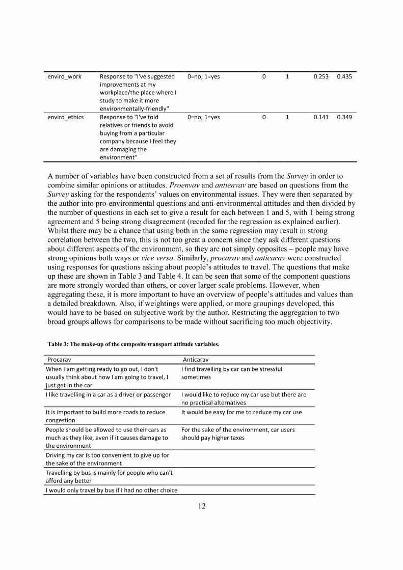
A number of variables have been constructed from a set of results from the Survey in order to

combine similar opinions or attitudes. Proenvav and antienvav are based on questions from the

Survey asking for the respondents’ values on environmental issues. They were then separated by

the author into pro-environmental questions and anti-environmental attitudes and then divided by

the number of questions in each set to give a result for each between 1 and 5, with 1 being strong

agreement and 5 being strong disagreement (recoded for the regression as explained earlier).

Whilst there may be a chance that using both in the same regression may result in strong

correlation between the two, this is not too great a concern since they ask different questions

about different aspects of the environment, so they are not simply opposites – people may have

strong opinions both ways or vice versa. Similarly, procarav and anticarav were constructed

using responses for questions asking about people’s attitudes to travel. The questions that make

up these are shown in Table 3 and Table 4. It can be seen that some of the component questions

are more strongly worded than others, or cover larger scale problems. However, when

aggregating these, it is more important to have an overview of people’s attitudes and values than

a detailed breakdown. Also, if weightings were applied, or more groupings developed, this

would have to be based on subjective work by the author. Restricting the aggregation to two

broad groups allows for comparisons to be made without sacrificing too much objectivity.

Table 3: The make-up of the composite transport attitude variables.

Procarav Anticarav

When I am getting ready to go out, I don't

usually think about how I am going to travel, I

just get in the car

I find travelling by car can be stressful

sometimes

I like travelling in a car as a driver or passenger I would like to reduce my car use but there are

no practical alternatives

It is important to build more roads to reduce

congestion

It would be easy for me to reduce my car use

People should be allowed to use their cars as

much as they like, even if it causes damage to

the environment

For the sake of the environment, car users

should pay higher taxes

Driving my car is too convenient to give up for

the sake of the environment

Travelling by bus is mainly for people who can't

afford any better

I would only travel by bus if I had no other choice

13

Table 4: The make-up of the composite environmental value variables.

Proenvav Antienvav

We are close to the limit of the number of

people the earth can support

The so-called 'environmental crisis' facing

humanity has been greatly exaggerated

When humans interfere with nature it often

produces disastrous consequences

Humans are capable of finding ways to

overcome the world's environmental problems

Humans are severely abusing the environment Scientists will find a solution to global warming

without people having to make big changes to

their lifestyles

The Earth has very limited room and resources Humans were meant to rule over the rest of

nature

If things continue on their current course, we

will soon experience a major environmental

disaster

It would embarrass me if my friends thought my

lifestyle was purposefully environmentally

friendly

I sometimes feel guilty about doing things that

harm the environment

Being green is an alternative lifestyle it's not for

the majority

The government is doing a lot to tackle climate

change

I find it hard to change my habits to be more

environmentally-friendly

If government did more to tackle climate

change, I'd do more too

Any changes I make to help the environment

need to fit in with my lifestyle

I do worry about the changes to the countryside

in the UK and the loss of native animals and

plants

I need more information on what I could do to

be more environmentally friendly

So many people are environmentally-friendly

these days, it does make a difference

The environment is a low priority for me

compared with a lot of other things in my life

It's only worth doing environmentally-friendly

things if they save you money

Climate Change is beyond control - it's too late

to do anything about it

The effects of climate change are too far in the

future to really worry me

It's not worth me doing things to help the

environment if others don't do the same

It's not worth Britain trying to combat climate

change, because other countries will just cancel

out what we do

It takes too much effort to do things that are

environmentally friendly

I'd struggle to find the time to be any more

environmentally-friendly than I am now

The other composite variable is labelled behavioursum. This is created by summing the binary

responses to five questions about people’s environmental behaviour, and has two functions. The

first is to see if people have coherent behaviours amongst travel-to-work decisions and the five

given here; the second is to measure people’s environmental values through revealed responses.

The five questions are shown in Table 2, and are enviro_talk, enviro_persuade, enviro_work,

enviro_ethics. It can be seen that while 31% of respondents claim they often talk to friends and

14

family about environmental behaviours, only 14% have spoken to them about purchasing from

particular companies. The composite variable will be included in one set of regressions

(multinomial logit and probit) and in a second set the variables will be included separately too

see if there is any individual significance. Black et al (2001) used factor analysis in compiling

sets of responses, but still adjusted these manually after inconclusive results, which is why the

method was not used in this research.

RESULTS

Multinomial Regression

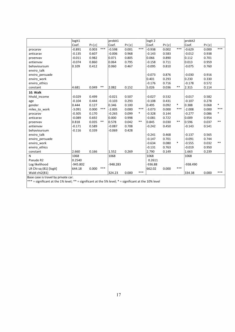
The results of four regressions are shown in Table 5. Logit1 and Probit1 were run with

behavioursum as a composite variable, and Logit2 and Probit2 include the components of

behavioursum as separate variables. All the regressions are multinomial, with driving as the base

case; positive coefficients imply that an increase in the variable means an increase in the

likelihood of an individual taking that form of transport relative to driving. Each of the

regressions is jointly significant at the 1% level as shown by the LR chi-squared or Wald chi-

squared statistic.

The regression shows that some modes of transport are more significantly estimated than others.

In particular, bus, rail and cycling all have a large number of significant variables at the 5% level

or higher. This is perhaps because they have the greater number of responses, or because they are

most affected by age, distance and environmental considerations. A third reason could be is that

over a range of distances to work, they are the closest alternatives to driving.

Income is, perhaps surprisingly, not significant (at the 10% level or better) for most of the

transport modes, except for rail, light rail and motorbike. This is perhaps because rail and light

rail are comparatively more expensive than other substitutes in the areas where these are option.

Age is a more significant variable, with older people more likely to drive than to take most of the

other options. Gender shows some interesting characteristics; it is not usually significant but

females are more likely to be driven by another member of the household, and males more likely

to cycle.

15

Table 5: Results of regressions

logit1 probit1 logit 2 probit2

Coef. P>|z| Coef. P>|z| Coef. P>|z| Coef. P>|z|

2. Lift Share (as driver)

hhold_income -0.036 0.536 -0.013 0.703 -0.036 0.532 -0.013 0.697

age -0.459 0.019 ** -0.312 0.004 *** -0.460 0.019 ** -0.307 0.005 ***

gender 0.857 0.031 ** 0.473 0.034 ** 0.881 0.028 ** 0.487 0.031 **

miles_to_work -0.226 0.076 * -0.186 0.011 ** -0.228 0.073 * -0.190 0.009 ***

procarav -0.914 0.006 *** -0.637 0.001 *** -0.871 0.008 *** -0.620 0.001 ***

anticarav 0.596 0.040 ** 0.349 0.029 ** 0.583 0.045 ** 0.348 0.029 **

proenvav 0.672 0.212 0.412 0.185 0.605 0.257 0.380 0.217

antienvav 0.515 0.233 0.382 0.125 0.584 0.171 0.420 0.089 *

behavioursum -0.224 0.189 -0.127 0.197

enviro_talk -0.139 0.744 -0.079 0.748

enviro_persuade 0.024 0.958 0.020 0.943

enviro_work -0.306 0.490 -0.191 0.449

enviro_ethics -0.179 0.740 -0.151 0.639

constant -4.382 0.093 * -2.576 0.087 * -4.589 0.076 * -2.706 0.070 *

3. Lift Share (as passenger)

hhold_income 0.016 0.820 0.015 0.689 0.021 0.758 0.019 0.615

age -0.810 0.002 *** -0.470 0.001 *** -0.787 0.002 *** -0.467 0.001 ***

gender -0.787 0.113 -0.397 0.126 -0.684 0.172 -0.348 0.195

miles_to_work 0.049 0.718 -0.007 0.922 0.062 0.646 0.010 0.901

procarav -0.492 0.213 -0.439 0.046 ** -0.522 0.193 -0.454 0.044 **

anticarav 0.421 0.222 0.241 0.199 0.469 0.175 0.280 0.145

proenvav -0.259 0.671 -0.081 0.815 -0.325 0.606 -0.134 0.707

antienvav 0.491 0.358 0.348 0.231 0.576 0.286 0.393 0.187

behavioursum -0.040 0.846 -0.026 0.817

enviro_talk -0.042 0.937 -0.090 0.757

enviro_persuade 0.013 0.984 0.039 0.910

enviro_work -1.287 0.098 * -0.710 0.069 *

enviro_ethics 0.831 0.144 0.498 0.125

constant -0.408 0.895 -0.487 0.773 -0.764 0.808 -0.671 0.698

4. Motorcycle, scooter,

moped

hhold_income 0.333 0.056 * 0.148 0.053 * 0.324 0.061 * 0.144 0.065 *

age -0.337 0.455 -0.198 0.355 -0.405 0.370 -0.220 0.303

gender -0.224 0.822 -0.128 0.787 -0.391 0.695 -0.160 0.739

miles_to_work -0.071 0.804 -0.060 0.665 -0.087 0.764 -0.048 0.736

procarav 0.092 0.910 -0.062 0.880 0.001 0.999 -0.126 0.756

anticarav -0.794 0.263 -0.314 0.359 -0.857 0.222 -0.336 0.336

proenvav 2.113 0.126 1.000 0.139 2.120 0.124 1.037 0.122

antienvav -0.602 0.584 -0.100 0.854 -0.850 0.458 -0.231 0.683

behavioursum 0.413 0.229 0.206 0.249

enviro_talk 0.561 0.627 0.374 0.482

enviro_persuade -0.323 0.785 -0.200 0.740

enviro_work 1.084 0.304 0.425 0.382

enviro_ethics -0.033 0.979 -0.130 0.843

constant -11.164 0.094 * -5.912 0.070 * -9.338 0.164 -5.242 0.104

5. Taxi

hhold_income -0.103 0.504 -0.022 0.754 -0.099 0.528 -0.021 0.770

age -1.026 0.088 * -0.512 0.060 * -1.018 0.090 * -0.504 0.066 *

gender 0.649 0.502 0.176 0.700 0.646 0.508 0.228 0.635

miles_to_work -0.406 0.230 -0.255 0.112 -0.396 0.254 -0.243 0.143

procarav 0.900 0.290 0.377 0.401 0.943 0.269 0.366 0.414

anticarav -1.164 0.096 * -0.533 0.125 -1.159 0.094 * -0.564 0.112

proenvav -0.327 0.782 0.124 0.832 -0.377 0.756 0.069 0.910

antienvav 0.470 0.587 0.325 0.472 0.452 0.621 0.363 0.439

16

logit1 probit1 logit 2 probit2

Coef. P>|z| Coef. P>|z| Coef. P>|z| Coef. P>|z|

behavioursum 0.426 0.287 0.216 0.284

enviro_talk 0.947 0.361 0.515 0.320

enviro_persuade 0.271 0.841 0.223 0.722

enviro_work -0.027 0.982 -0.084 0.883

enviro_ethics 0.750 0.548 0.290 0.644

constant -1.309 0.825 -2.106 0.476 -1.267 0.834 -2.039 0.498

6. Bus

hhold_income -0.027 0.576 -0.012 0.668 -0.033 0.500 -0.016 0.597

age -0.398 0.011 ** -0.281 0.003 *** -0.390 0.013 ** -0.279 0.003 ***

gender 0.253 0.406 0.121 0.522 0.261 0.398 0.128 0.509

miles_to_work -0.217 0.031 ** -0.188 0.003 *** -0.215 0.033 ** -0.187 0.003 ***

procarav -1.242 0.000 *** -0.801 0.000 *** -1.212 0.000 *** -0.784 0.000 ***

anticarav 0.556 0.018 ** 0.312 0.025 ** 0.556 0.020 ** 0.318 0.023 **

proenvav 0.827 0.054 * 0.507 0.052 * 0.809 0.058 * 0.508 0.052 *

antienvav 1.092 0.002 *** 0.638 0.003 *** 1.070 0.002 *** 0.633 0.003 ***

behavioursum -0.149 0.275 -0.079 0.349

enviro_talk -0.187 0.601 -0.081 0.713

enviro_persuade -0.800 0.094 * -0.455 0.101

enviro_work 0.059 0.867 -0.009 0.968

enviro_ethics 0.382 0.349 0.254 0.331

constant -4.344 0.037 ** -2.333 0.067 * -4.388 0.037 ** -2.424 0.058 *

7. Train

hhold_income 0.156 0.007 *** 0.086 0.013 ** 0.160 0.006 *** 0.088 0.011 **

age -0.461 0.023 ** -0.363 0.003 *** -0.463 0.023 ** -0.367 0.003 ***

gender -0.214 0.571 -0.223 0.339 -0.191 0.619 -0.219 0.357

miles_to_work 0.446 0.000 *** 0.242 0.000 *** 0.453 0.000 *** 0.246 0.000 ***

procarav -1.325 0.000 *** -0.911 0.000 *** -1.396 0.000 *** -0.944 0.000 ***

anticarav 0.488 0.097 * 0.270 0.130 0.530 0.075 * 0.291 0.107

proenvav -0.734 0.150 -0.446 0.146 -0.736 0.148 -0.438 0.155

antienvav 0.304 0.502 0.290 0.272 0.325 0.479 0.256 0.339

behavioursum 0.043 0.775 0.028 0.766

enviro_talk 0.095 0.824 0.012 0.963

enviro_persuade 0.296 0.512 0.156 0.588

enviro_work -0.263 0.529 -0.145 0.576

enviro_ethics -0.432 0.427 -0.305 0.377

constant -0.852 0.740 -0.062 0.968 -0.844 0.743 0.081 0.958

8. Underground, tram, light

railway

hhold_income 0.213 0.006 *** 0.115 0.005 *** 0.230 0.004 *** 0.121 0.004 ***

age -0.301 0.243 -0.253 0.057 * -0.302 0.246 -0.245 0.067 *

gender -0.718 0.190 -0.374 0.189 -0.641 0.248 -0.322 0.270

miles_to_work 0.056 0.693 -0.002 0.985 0.067 0.646 0.009 0.912

procarav -1.074 0.018 ** -0.746 0.003 *** -1.178 0.010 ** -0.817 0.002 ***

anticarav 0.494 0.210 0.237 0.245 0.538 0.176 0.269 0.193

proenvav 1.161 0.093 * 0.628 0.103 1.146 0.099 * 0.624 0.110

antienvav 1.285 0.022 ** 0.737 0.014 ** 1.309 0.022 ** 0.777 0.013 **

behavioursum 0.062 0.763 0.042 0.717

enviro_talk 0.296 0.606 0.162 0.600

enviro_persuade 0.457 0.462 0.189 0.575

enviro_work -1.038 0.135 -0.450 0.190

enviro_ethics -0.352 0.662 -0.247 0.563

constant -9.688 0.005 *** -4.842 0.007 *** -9.699 0.006 *** -4.934 0.007 ***

9. Cycle

hhold_income 0.071 0.164 0.047 0.133 0.070 0.167 0.048 0.126

age -0.420 0.014 ** -0.272 0.009 *** -0.440 0.011 ** -0.283 0.007 ***

gender -0.872 0.014 ** -0.485 0.021 ** -0.902 0.011 ** -0.496 0.019 **

miles_to_work -0.907 0.000 *** -0.582 0.000 *** -0.908 0.000 *** -0.588 0.000 ***

17

logit1 probit1 logit 2 probit2

Coef. P>|z| Coef. P>|z| Coef. P>|z| Coef. P>|z|

procarav -0.891 0.003 *** -0.598 0.001 *** -0.938 0.002 *** -0.629 0.000 ***

anticarav -0.135 0.607 -0.006 0.968 -0.143 0.583 -0.012 0.938

proenvav -0.011 0.982 0.071 0.805 0.066 0.890 0.112 0.701

antienvav -0.074 0.860 0.064 0.795 -0.158 0.711 0.013 0.959

behavioursum 0.109 0.412 0.060 0.467 -0.095 0.810 -0.075 0.760

enviro_talk

enviro_persuade -0.073 0.876 -0.030 0.916

enviro_work 0.401 0.293 0.230 0.330

enviro_ethics -0.176 0.716 -0.178 0.572

constant 4.681 0.049 ** 2.082 0.152 5.026 0.036 ** 2.315 0.114

10. Walk

hhold_income -0.029 0.499 -0.021 0.507 -0.027 0.532 -0.017 0.582

age -0.104 0.444 -0.103 0.293 -0.108 0.431 -0.107 0.278

gender 0.444 0.127 0.346 0.100 0.495 0.092 * 0.388 0.068 *

miles_to_work -3.091 0.000 *** -2.005 0.000 *** -3.073 0.000 *** -2.008 0.000 ***

procarav -0.305 0.170 -0.265 0.099 * -0.328 0.144 -0.277 0.086 *

anticarav -0.089 0.692 0.000 0.998 -0.081 0.722 0.009 0.954

proenvav 0.818 0.035 ** 0.578 0.042 ** 0.845 0.030 ** 0.596 0.037 **

antienvav -0.171 0.589 -0.087 0.708 -0.242 0.450 -0.143 0.541

behavioursum -0.116 0.339 -0.069 0.428

enviro_talk -0.241 0.468 -0.137 0.565

enviro_persuade -0.147 0.701 -0.091 0.744

enviro_work -0.634 0.080 * -0.555 0.032 **

enviro_ethics -0.131 0.763 -0.019 0.950

constant 2.660 0.166 1.552 0.269 2.790 0.149 1.663 0.239

N 1068 1068 1068 1068

Pseudo R2 0.2540 0.2611

Log likelihood -945.802 -948.283 -936.88 -938.490

LR Chi-sq (81) [logit] 644.18 0.000 *** 662.02 0.000 ***

Wald chi2(81) 324.23 0.000 *** 334.38 0.000 ***

Base case is travel by private car.

*** = significant at the 1% level; ** = significant at the 5% level; * = significant at the 10% level

18

Distance to work is significant, particularly for public transport and for non-motorised

transport. The results agree with the idea that there are structural limits to cycling,

walking and using buses, and that trains are considered better for longer distances.

Looking at option 2, lift sharing with someone from your household, it can be seen

that procarav is negative and strongly significant, and anticarav is positive and

significant at the 5% level. This suggests that within households, people who do not

like driving are more likely to be driven than to drive, which makes clear sense. In

most cases where attitudes towards or against cars are significant, procarav is more

significant and larger than anticarav. That is, pro-car attitudes are more powerful

indicators of drivers than anti-car attitudes are indicators of non-drivers. For example,

in the case of travelling by train, positive attitudes towards driving are a stronger

indicator of someone driving rather than taking the train compared with anti-car

attitudes which point towards using the train. Attitudes towards cars have little impact

on people choosing to walk, but pro-environmental values are significant at the 5%

level and positive for all the regressions.

However, environmental considerations are not important under any of the

regressions. This gives support to the theory that attitudes are more important

predictors of behaviour than values. The environmental value variables are not very

significant in most transport decisions except in the choice to walk – and here the car

attitudes have little significance. Also of note are the environmental values variables

for bus and light railway. Here, they are significant but in both cases, both the pro-

and anti-environmental values are positive. As was stated earlier in the methodology

section, this is not necessarily a mistake, since the variables were constructed to allow

a range of values to be expressed under pro- and anti- labels. It could be that people

who take these methods develop stronger opinions, due perhaps to encounters with

bus fumes, advertising or other people.

Finally, both the regressions that looked at behavioursum as a single variable and as

separate variables found these to be largely insignificant predictors of travel choice.

Where there is some significance at the 10% level of better, there is a negative sign on

the coefficient. This suggests that people who drive instead of walk, take the bus or

lift share as a passenger are more likely to have spoken to other people or their work

about being more environmentally friendly. Whether this is a displacement effect

whereby people feel guilty for driving so speak up (or tell the interviewer they have

done so) is impossible to tell from the dataset. Since the evidence is fairly weak, it is

difficult to say how robust this observation is.

Overall, the results are reasonably strong and coherent, and show that people are more

likely to choose their method of commuting based on attitudes to transport than

environmental values. In terms of sensitivity analysis, the logit and probit results

show similar significances and signs to each other, which suggests that the results are

not highly sensitive to the underlying regression analysis used.

Ordered Regression

As a second level of sensitivity analysis, and to explore the data further, a simple

ordered regression was run. In this case, instead of the dependent variable being

different types of transport where the order does not matter, the levels of the

dependent variable are ordered or ranked. The differences between the levels of the

variable are still meaningless however, so the ranking is ordinal not cardinal. To

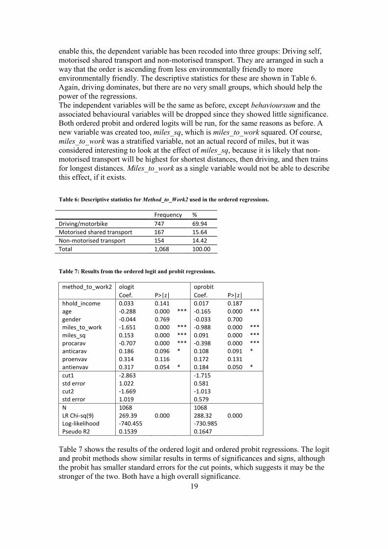
19

enable this, the dependent variable has been recoded into three groups: Driving self,

motorised shared transport and non-motorised transport. They are arranged in such a

way that the order is ascending from less environmentally friendly to more

environmentally friendly. The descriptive statistics for these are shown in Table 6.

Again, driving dominates, but there are no very small groups, which should help the

power of the regressions.

The independent variables will be the same as before, except behavioursum and the

associated behavioural variables will be dropped since they showed little significance.

Both ordered probit and ordered logits will be run, for the same reasons as before. A

new variable was created too, miles_sq, which is miles_to_work squared. Of course,

miles_to_work was a stratified variable, not an actual record of miles, but it was

considered interesting to look at the effect of miles_sq, because it is likely that non-

motorised transport will be highest for shortest distances, then driving, and then trains

for longest distances. Miles_to_work as a single variable would not be able to describe

this effect, if it exists.

Table 6: Descriptive statistics for Method_to_Work2 used in the ordered regressions.

Frequency %

Driving/motorbike 747 69.94

Motorised shared transport 167 15.64

Non-motorised transport 154 14.42

Total 1,068 100.00

Table 7: Results from the ordered logit and probit regressions.

method_to_work2 ologit oprobit

Coef. P>|z| Coef. P>|z|

hhold_income 0.033 0.141 0.017 0.187

age -0.288 0.000 *** -0.165 0.000 ***

gender -0.044 0.769 -0.033 0.700

miles_to_work -1.651 0.000 *** -0.988 0.000 ***

miles_sq 0.153 0.000 *** 0.091 0.000 ***

procarav -0.707 0.000 *** -0.398 0.000 ***

anticarav 0.186 0.096 * 0.108 0.091 *

proenvav 0.314 0.116 0.172 0.131

antienvav 0.317 0.054 * 0.184 0.050 *

cut1 -2.863 -1.715

std error 1.022 0.581

cut2 -1.669 -1.013

std error 1.019 0.579

N 1068 1068

LR Chi-sq(9) 269.39 0.000 288.32 0.000

Log-likelihood -740.455 -730.985

Pseudo R2 0.1539 0.1647

Table 7 shows the results of the ordered logit and ordered probit regressions. The logit

and probit methods show similar results in terms of significances and signs, although

the probit has smaller standard errors for the cut points, which suggests it may be the

stronger of the two. Both have a high overall significance.

20

Income and gender are insignificant, but the other personal and structural variables

are. Both miles_to_work and miles_sq are significant, and have different signs,

suggesting that over medium distances, people are more likely to drive and over

longer distances public transport it more used. Older people are more likely to use less

environmentally friendly transport.

Pro- and anti- car attitudes are both significant, and with the expected signs. Procarav

is however, both larger in scale and significance than anticarav. This is either due to

the much larger amount of people driving than using other methods, thus making the

variables which are linked to driving have a stronger effect.

Environmental values are much less strong than attitudes towards transport, and only

anti-environmental opinions have a significant effect, but this is the opposite of what

would be expected. Both the probit and logit show antienvav to have a positive effect

on transport decisions, at a significant of just over 5%. This perhaps shows the

weakness of using composite variables to quantify values. For example, the variable

antienvav contains statements such as “It's only worth doing environmentally-friendly

things if they save you money” which would perhaps be pro-cycling or pro-walking.

It also contains statements which have a certain degree of mutual inconsistency, for

example, “Climate Change is beyond control - it's too late to do anything about it,”

and “The effects of climate change are too far in the future to really worry me.”

DISCUSSION

The results showed that distance to work was a crucial variable in people’s selection

of transport methods particularly in comparing driving with travelling by train, foot or

bicycle. This is not a surprising result, and including the distance to work squared

term in the ordered regression highlighted the importance of different distances.

However, between different options that cover a similar distance, such as lift-sharing,

bus motorcycling, or driving, distance is not a significant variable. Indeed, in these

cases, the other variables are rarely significant as well. This suggests that structural

limits are more important than the attitudinal and value aspects.

Another interesting point is that, as seen in Table 5, there are a number of significant

factors in people’s decision to lift share as driver compared to driving alone, but these

are not so significant in the sharers who do not drive. Again, this could be because

people feel (structurally) forced to drive, due to distance or lack of public transport,

but dislike driving so take company. Environmental values are not important in

people’s decision to lift share.

One trend that was repeated for most of the regressions was that attitudes were a more

significant indicator than values. Generally, the environmental values had

insignificant or vague impacts on travel behaviour, whereas attitudes were a common

predictor of behaviour. In particular, anti-car attitudes predict people are more likely

to use non-driving methods, or at least to car-share. This may seem too obvious to

need studying, but it is recognised that people may hold inconsistent or contradictory

attitudes. This study adds to the literature which notices the greater consistency

between attitudes and behaviour than values and behaviour. In a similar way, there are

only very weak links between stated environmental behaviour as shown by people’s

willingness to talk to others or their employers about the environment, and travel

behaviour. In economics, revealed behaviour is often felt to be a more reliable

21

indicator of preferences than stated behaviour, but here this suggests the opposite.

This could be because of the narrow range of environmental actions (as shown in

Table 2), all of which have a somewhat evangelical theme to them. That is, attempting

to persuade others to change their environmental behaviours shows a high level of

environmental concern, and so this variable does not capture the whole range of

environmental concerns/values which may lead to travel behaviour change. Inasmuch

as this variable is usable however, the results also add to the conclusion that values

have a low impact on behaviour, and that leads to the possibility of inconsistent

behaviours which would be difficult to sustain if the behaviour-value links were

stronger.

This research also suggests a number of policy-relevant results. Firstly, age was a

significant variable in people taking options other than driving alone. This suggests

that policy measures aimed at encouraging behavioural change should be age-

targeted. Obviously, policies cannot change people’s ages, but it can focus on older

age groups where there are larger numbers of people who are driving alone to work.

Policies to encourage lift sharing or public transport use could therefore aim at things

which these age groups prefer, such as comfort or flexibility. Further research would

therefore be needed to find out exactly what these preferences are. Also, the

significance of age suggests that in the long-run, the public may (if they keep their

current attitudes) become less car-centric. Also, policies could be aimed at

encouraging older people to cycle to work, for example, showing its health benefits.

The second policy relevant finding is that structural variables are important; in

particular, this research highlights the impact of the distances to work. Over short and

long distances, people are more likely to use more environmentally friendly methods,

but over medium distances people are more inclined to drive alone to work. In the

long-term, people could be encouraged to work nearer home, or live nearer work, but

this would need a large scale plan at both the national and local levels. A more

workable policy suggestion would be to increase people’s options for travelling a

medium distances. Making driving alone less attractive and shared transport more

attractive would help shift people’s travel choices towards more environmentally

friendly modes of transport over the medium distances. Again, the precise range of

factors that would persuade people to change is not disclosed by this research.

Thirdly, and most importantly, this research shows that attempts to change people’s

values – whether through information or education – are likely to have a low impact.

The variables in the regressions that proxied environmental values were largely

insignificant or vague in their impact on people’s choice of commuting method.

Limited resources would best be put towards the policies recommended above, rather

than in attempting to change beliefs or values. Educational or informational policies

that changed attitudes would however, have more success in changing behaviour.

Looking back at Table 5, the issues raised in the procarav column could be addressed,

for example by changing perceptions of bus travel. Of course, changing people’s

perceptions is different to changing the actual experience of bus travel – not only

would buses have to change, this would have to be communicated to drivers on a level

that will change their mentality towards travelling by bus.

22

CONCLUSION

This research paper has used econometrics to analyse what affects the choice of

transport method people take to work. Using data from Defra’s 2007 Survey of

Attitudes and Behaviours in relation to the Environment, (Defra, 2007) and based on a

framework developed from both the economic and psychological literature, the

research found a number of significant factors in this decision. Perhaps more

interestingly, income and environmental values were not significant in people’s travel

choices. Attitudes to car travel and distance travelled to work were both important in

most travel decisions.

Distance to work, and later distance squared, were both significant. This suggests that

structural variables are key to individuals’ travel decisions, but the dataset lacked

information about other structural variables that could be used, such as proximity of a

public transport route to the individual’s work or the need to share commuting with

other tasks such as the school run or shopping. Costs of travel also were not known. It

may seem a large assumption to extrapolate from the significance of distance to work

to the statement that structural variables are key, but this is backed up by the

literature, for example, Parkin et al’s (2008) findings on the likelihood of cycling to

work in various UK regions.

Another possible weakness in the dataset was the lack of local variables, such as

hilliness or vehicle related crime rates. Knowing these would probably have revealed

more information about travel decisions as they are highly likely to influence

behaviour. However, as the research did not aim to find every influential factor, but

rather to assess the impact of environmental values, this is not a major weakness.

Finally, the results depend to quite a large extent on the formulation of the variables

that measured environmental values, environmental behaviour and transport attitudes.

These were taken from the 2007 Survey and compiled to make composite variables,

which avoided having too many variables in the equation, and allowed for a range of

pro-environmental opinions (for example) being measured in one variable. This is a

good thing, because people can have pro-environmental opinions in one respect, such

as concern over climate change, but not in others such as the need for recycling.

Compiling these attitudes and values into single variables allows the focus of the

paper to remain focussed.

Overall, this paper presents an important synthesis of two strands of the

environmental literature, from economics and psychology. The results shed light on

transport behaviours and show that psychological insights about people’s behaviours

and attitudes can be integrated into an economic framework. Looking ahead, more

work is needed in compiling attitudinal and value-based variables for future studies.

In particular, it remains open to debate whether integrating a wide range of values or

attitudes into one or two variables is a successful methodology, or whether tools such

as factor analysis (such as Black et al, 2001) present a better way ahead. Future

research could also look into the effectiveness of policies that are aimed at changing

behaviour through changing attitudes. Whilst research like this paper suggests that

this would be an effective strategy, the implementation and costs of such policies may

make them unworkable. However, there is a growing body of literature around such

questions, and this paper adds a useful contribution.

23

REFERENCES

Bagley, M.N and P.L Mokhtarian (2002) “The impact of residential neighbourhood

type on travel behaviour: A structural equations modeling approach”, The

Annals of Regional Science 36:279-297.

Barr, S., A.W Gilg and N.J Ford (2001) “Differences between household waste

reduction, reuse and reduction behaviour: A study of reported behaviours,

intentions and explanatory variables”, Environmental and Waste Management

4(2): 69-82.

Black, C., A. Collins and M. Snell (2001) “Encouraging walking: The case of

journey-to-school trips in compact urban areas”, Urban Studies 38:1121-1141.

Bryman, A. (2004) Social Research Methods, 2nd ed. Oxford University Press: Great

Britain.

Cervero, R., 2002, ``Built environment and mode choice: toward a normative

framework'' Transportation Research D 7:265-284.

Cervero, R., and C. Radisch (1996) “Travel choices in pedestrian versus automobile

oriented neighborhoods”, Transport Policy 3(3):127–141.

Davies, J., G.R Foxall and J. Pallister (2002) “Beyond the intention-behaviour

mythology: An integrated model of recycling”. Marketing Theory 2(1):29-113.

Defra (2007) Survey of Attitudes and Behaviours in Relation to the Environment.

Project homepage at

http://www.defra.gov.uk/environment/statistics/pubatt/index.htm. Accessed

15.12.08.

Diekmann, A., and P. Preisendörfer (2003) “Green and greenback: The behavioural

effects of environmental attitudes in low-cost and high-cost situations”.

Rationality and Society 15(4):441-472.

Dijst, M., S. Farag and T. Schwanen (2008) “A comparative study of attitude theory

and other models for understanding travel behaviour”, Environment and

Planning A 40:831-847.

Eagly, A.H and P. Kulesa (1997) “Attitudes, Attitude Structure and Resistance to

Change: Implications for Persuasion on Environmental Issues” In: Bazerman,

M.N, D.M Messick, A.E Tenbrunsel and K.A Wade-Benzoni (eds.)

Environment, Ethics and Behaviour: New Lexington Press: USA.

Feldman, O., and D. Simmonds (2007) Household Location Modelling. David

Simmonds Consultancy, with University of Leeds School of Geography,

University College London and MVA for the Department for Transport, UK.

Report available online at http://www.dft.gov.uk/pgr/economics/rdg/hlm/

24

Grob, A. (1995) “A structural model of environmental attitudes and behaviour”,

Journal of Environmental Psychology 15: 209-220.

Gujurati, D.N (1995) Basic Econometrics. International Edition. McGraw-Hill:

Singapore.

Heij, C., P. de Boer, P.H Franses, T. Kloek and H.K van Dijk (2004) Econometric

Methods with Applications in Business and Econometrics. Oxford University

Press: USA.

Joireman, J.A, T.P Lasane, J. Bennett, D. Richards, and S. Solaimani (2001)

“Integrating social value orientation and consideration of future consequences

within the extended norm activation model of proenvironmental behaviour”.

British Journal of Social Psychology 40: 133-155.

Joireman, J.A., P.A.M Van Lange and M. Van Vught (2004) “Who cares about the

environmental impact of cars? Those with an eye toward the future”.

Environment and Behaviour 36:187-206.

Katz, D. (1960) “The functional approach to the study of attitudes” Public Opinion

Quarterly 24:163-204.

Kitamura, R., P.L Mokhtarian and L Laidet (1997) “A micro-analysis of land use and

travel in five neighbourhoods in the San Francisco Bay Area”. Transportation

24(2):125-158.

McFadden (1974) “The measurement of urban traffic demand” Journal of Public

Economics 3:303-328.

Parkin, J., M. Wardman and M. Page (2008) “Estimation of the determinants of

bicycle mode share for the journey to work using census data”. Transportation

35:93-109.

Poortinga, W., L. Steg and C. Vlek (2004) “Values, environmental concern and

environmental behaviour: A study into household energy use”. Environment

and Behaviour 36(1): 70-93.

Schultz, P.W., S. Oskamp and T. Mainieri (1995) “Who recycles and when? A review

of personal and situational factors”. Journal of Environmental Psychology

15:105-121.

Schwanen, T., and P.L Mokhtarian (2005) “What if you live in the wrong

neighbourhood? The impact of residential neighbourhood type dissonance on

distance travelled”. Transportation Research Part D 10(2): 127-151.

Stanbridge, K., G. Lyons and S. Farthing (2004) Travel Behaviour Change and

Residential Location. Paper presented at the 3rd International Conference of

Traffic and Transport Psychology, 5-9 September, Nottingham, UK.

25

Van Lange, P.A.M., M. Van Vugt, R.M Meertens and R.A.C Ruiter (1998) “A social

dilemma analysis of commuting preferences: The roles of social value

orientation and trust”. Journal of Applied Social Psychology 28:796-820.

Van Vugt, M., P.A.M Van Lange and R.M Meertens (1996) “Commuting by car or

public transportation? A social dilemma analysis of travel mode judgments”.

European Journal of Social Psychology 26:373-395.

Van Vugt, M., R.M Meertens and P.A.M Van Lange (1995) “Car or public

transportation? The role of social orientations in a real-life social dilemma”.

Journal of Applied Social Psychology 25:258-278.

Weeks, M. (1997) “The multinomial probit model revisited: A discussion of

parameter estimability, identification and specification testing”. Journal of

Economic Surveys 11(3): 297-320.