optimizing coordination strategies in a real supply chain ... · developing new coordination...
TRANSCRIPT

Optimizing Coordination Strategies in a Real Supply Chain: Simulation Approach
Von der Fakultät für Ingenieurwissenschaften, Abteilung Maschinenbau der
Universität Duisburg-Essen
zur Erlangung des akademischen Grades
DOKTOR-INGENIEUR
genehmigte Dissertation
von
Tarak Ali Housein
aus
Benghazi / Libyen
Referent: Univ.-Prof. Dr.-Ing. Bernd Noche
Korreferent: Univ.-Prof. Dr.-Ing. Uwe Meinberg
Tag der mündlichen Prüfung: 12.09.2007

ABSTRACT OF THE DISSERTATION
In recent years the interest in the supply chain coordination field has been
growing, both among companies and researchers, particularly in the area of
transportations systems and logistics management. Many companies realize
that coordinating supply chain activities can maximize the performance of the
supply chain, through the minimization of the system-wide costs while still
satisfying service level requirements. The coordination of inventory and
distribution (transportation) activities are the effective key for efficient
coordination of the supply chain. Therefore, this dissertation deals mainly with
developing new coordination distribution strategies that coordinate the inventory
and transportation activities and optimize the performance of the supply chain.
These strategies are evaluated and their applications are reported using the
real-life supply chain network which motivated this research. In this dissertation,
a real life food Supply Chain company located in a European country was
considered for more detailed studies. Since the real supply chain being
modeled and the problem of coordinating two activities are so complex that
optimal solutions are very hard to obtain, most of the study models consider
simple networks and make many assumptions to simplify the problem, for
example, considering only one item in a static inventory system. Thus, it can be
solved by exact algorithms (mixed integer programming) and heuristic solution
approaches.
Generally to solve such coordinated problems optimally is not easy due to its
combinatorial nature, especially when many strategies are involved. Simulation
models that permit user interaction and take into account the dynamics of the
system are capable of characterizing system performance for coordinated and
integrated models.
A discrete simulation model integrated with C++ program was constructed
specifically for modeling this real supply chain. The simulation model was

___________________________________________________________________ ii
validated by comparing the simulation results with the real data provided by the
company. Then the simulation is extended to model and implement the new
coordination distribution strategies. The new strategies are designed based on
new trends and a new prescriptive of the Supply Chain. To show the
importance and the value of the coordination strategies, uncoordinated
strategies which were designed based on the item classification approaches
(ABC & XYZ classifications) are presented and implemented by the developed
simulation model. These uncoordinated strategies are evaluated to compare
them with the developed new coordination strategies. The new trends which are
considered in designing the coordination strategies are, for example, the
shipment consolidation concepts, advance demand information technology, and
vendor managed inventory (VMI) programs. All the mentioned trends are
implemented and realized in this work.
This dissertation presents two new shipment consolidation concepts for
constructing new coordination distribution strategies. These two are the "Item
classification consolidation concept" and "N-days forecasted demand
consolidation concept". The first consolidation concept is developed based on
the item classification concept and the second consolidation concept is
developed based on the advance demand information technology. The
problems such as the residual stock resulting from applying or using the
coordination strategies are interpreted and discussed. Moreover, these two
consolidation concepts are integrated with the VMI programs to construct more
appropriate and efficient coordination strategies between the inventory policies
and transportation strategies.
To evaluate the effectiveness of the coordination strategies, a number of
measures of performance have been selected. These measures are the
logistics costs and the customer satisfaction (responsiveness/backorders).
Many simulation results are collected and analyses have been made. These
results and analyses show that under the right conditions the value of
coordination can be extremely high. Also, the simulation results show that, the
coordination strategies are better than the uncoordinated strategies for
optimizing the system performance. Furthermore, the newly developed

___________________________________________________________________ iii
coordination strategies which incorporate the appropriate shipment
consolidation concepts, advanced information technology, and apply new
initiatives like VMI programs, are capable of reducing the system-wide costs
and improving the Supply Chain performances significantly. Finally, conclusions
and suggestions for future research have been presented.

___________________________________________________________________ iv
Dedication
TO
My mother, Halima My father, Prof. Ali
My wife, Ing. Khadiga My daughter Ala My daughter Arig
My daughter Farah My brothers and my sisters
Tarak Ali Housein

___________________________________________________________________ v
Acknowledgments
I wish to express my sincere gratitude to my supervisor Prof. Dr.-Ing. Bernd
Noche, for the may inspirational discussions and guidance throughout this work.
Special thanks to all academic and technical staff of Transportsysteme und
–logistik Institute for their many helpful suggestions and technical supports.
I wish to acknowledge my gratitude to the SimulationsDienstleistungsZentrum
GmbH for their support especially in applied simulation and optimization
methods for simulation studies for real life application.
Another special gratitude owes to my wife, from whom I always get support and
lovely care especially during my study here in Germany.
At last but not least, I would like to thank my family (mother, father, brothers,
and sisters) for their support all the way from the very beginning of my study.
I am thankful to all my family members for their thoughtfulness and
encouragement.
Duisburg, September 2007 Tarak Ali Housein

___________________________________________________________________
vi
Contents
1. Introduction ..................................................................................................................... 1
1.1. Definition of Supply Chain ................................................................................... 1
1.2. Coordination in Supply Chains ............................................................................. 4
1.3. Motivation ............................................................................................................. 7
1.4. Outline of the Thesis ............................................................................................. 7
2. Literature Review ............................................................................................................ 9
2.1. Overview of various approaches on the coordination and integrated problems in supply
chains 9
2.2. Overview of the supply Chain Simulation .......................................................... 16
2.3. Goals of the Dissertation ..................................................................................... 19
3. Modeling Coordination Strategies in Supply Chains Using Simulation: ...................... 21
A real-Life Case Study ........................................................................................................ 21
3.1. Introduction ......................................................................................................... 21
3.2. Simulation Model Description ............................................................................ 23
3.2.1. Model Elements........................................................................................... 26
3.2.2. Model Data .................................................................................................. 30
3.2.3. Model Output Reports ................................................................................. 36
3.3. Model Policies and Strategies ............................................................................. 42
3.3.1. Inventory Management Policies .................................................................. 43
3.3.2. Transportation Strategies............................................................................. 45
3.4. Model Implementation ........................................................................................ 46
3.5. Model Optimization............................................................................................. 49
3.6. A Real-Life Case Study....................................................................................... 50
3.6.1. A Real Distribution Supply Chain Description ........................................... 50
3.6.2. Model Data and Analysis ............................................................................ 52
3.6.3. Problem Description.................................................................................... 63
3.6.4. Simulation Model and Assumptions ........................................................... 64
3.6.5. Simulation Experiment and Results ............................................................ 65
3.7. Extended Studies and Models ............................................................................. 66
3.7.1. Investigation of Coordinating Distribution Strategies and Inventory Policies Study 67
3.7.2. Coordination Strategies Model Study II...................................................... 68
3.7.3. VMI-Programs Model Study II ................................................................... 76

___________________________________________________________________
vii
4. Design and Analysis of Uncoordinated Distribution Strategies:................................... 81
Item Classification approaches............................................................................................ 81
4.1. ABC Classification, XYZ, and ABC-XYZ Classification approaches ....... 81
4.1.1. ABC Classification...................................................................................... 81
4.1.2. XYZ Classification:..................................................................................... 86
4.2. Design of Uncoordinated Strategy Experiments ................................................. 92
4.2.1. Experiment ABC– Item Strategy (without Safety Stock) - (UCS- Expt 1): 93
4.2.2. Experiment ABC-Item Strategy (with Safety Stock) – (UCS- Expt 2): ...... 94
4.2.3. Experiment ABC- Item Strategy (minimize transportation) – (UCS- Expt 3):95
4.2.4. Experiment C- Item Allocation Strategy- (UCS- Expt 4): .......................... 96
4.2.5. Experiment XYZ-Item Strategy - (UCS- Expt 5):....................................... 97
4.2.6. Experiment Z- Item Allocation Strategy- (UCS- Expt 6): .......................... 97
4.2.7. Experiment ABC- XYZ - Combination Strategy- (UCS- Expt 7): ............. 98
4.2.8. Experiment ABC- XYZ – Combination Strategy (MIL) - (UCS- Expt 8):. 99
4.2.9. Experiment CSL (80%) ABC Item Strategy- (UCS- Expt 9): .................... 99
4.2.10. Experiment CSL (90%) ABC Item Strategy- (UCS-Expt 10): ................. 101
4.3. Performance Measures: ..................................................................................... 103
4.3.1. Total Transportation Cost (TTC):.............................................................. 103
4.3.2. Total Inventory Holding Cost (TIHC):...................................................... 104
4.3.3. Total Logistics Cost (TLC): ...................................................................... 104
4.3.4. Item Fill Rate Measures: ........................................................................... 104
4.3.5. Order Lines Fill Rate Measures:................................................................ 105
4.3.6. Order Fill Rate Measures: ......................................................................... 105
4.4. Experimental Simulation Results and Analysis ................................................ 106
4.4.1. Logistics Costs Analysis: .......................................................................... 108
4.4.2. Fill Rate Analysis: ..................................................................................... 115
4.4.3. Truck Utilization Analysis: ....................................................................... 120
5. Coordination Distribution Strategies:.......................................................................... 123
Design and Analysis .......................................................................................................... 123
5.1. Design of Coordination Strategy Experiments:................................................. 124
5.1.1. Coordination Strategy Experiments (1) - (CS1-Expt): .............................. 125
5.1.2. Coordination Strategy Experiments (2) - (CS2-Expt): .............................. 125
5.1.3. Coordination Strategy Experiments (3) - (CS3-Expt): .............................. 126
5.1.4. Coordination Strategy Experiments (4) - (CS4-Expt): .............................. 127

___________________________________________________________________
viii
5.1.5. Coordination Strategy Experiments (5) - (CS5-Expt): .............................. 127
5.1.6. Coordination Strategy Experiments (6) - (CS6-Expt): .............................. 128
5.1.7. Coordination Strategy Experiments (7) - (CS7-Expt): .............................. 128
5.2. Experimental Simulation Results ...................................................................... 129
5.2.1. Results of Coordination Strategy Experiments (1).................................... 130
5.2.2. Results of Coordination Strategy Experiments (2).................................... 131
5.2.3. Results of Coordination Strategy Experiments (3).................................... 132
5.2.4. Results of Coordination Strategy Experiments (4).................................... 133
5.2.5. Results of Coordination Strategy Experiments (5).................................... 134
5.2.6. Results of Coordination Strategy Experiments (6).................................... 135
5.2.7. Results of Coordination Strategy Experiments (7).................................... 136
5.3. Analysis of Simulation Results ......................................................................... 137
5.3.1. Logistics Costs and Fill Rate Analysis ...................................................... 137
5.3.2. Residual Stock Analysis ............................................................................ 151
5.3.3. Truck Utilization Analysis: ....................................................................... 157
6. Optimization of Coordination Strategies: Developing New ABC Classification ....... 160
6.1. New ABC Classification Model:....................................................................... 160
6.2. Experiments Designs ......................................................................................... 166
6.2.1. Experiment New-ABC-Item Uncoordinated Strategy - (UCS-N-Expt):... 167
6.2.2. Experiments New-ABC-Item Coordination Strategy (1) - (CS1-N-Expt):167
6.2.3. Experiments New-ABC-Item Coordination Strategy (2) - (CS2-N-Expt):169
6.3. Experimental Simulation Results and analysis.................................................. 170
6.3.1. Simulation Results and analysis of UCS-N-Expt & CS1-N-Expt Strategies170
6.3.2. Simulation Results and analysis of CS2-N-Expt Strategy ........................ 174
7. Optimization of Coordination Strategies Using Vendor-Managed Inventory (VMI) Programs
........................................................................................................................... 182
7.1. VMI-Programs Model: ...................................................................................... 182
7.2. Experiments Designs ......................................................................................... 183
7.2.1. VMI-Programs Uncoordinated Strategy - (UCS-V-Expt):........................ 184
7.2.2. VMI-Programs Coordination Strategy - (CS-V-Expt): ............................. 184
7.3. Experimental Simulation Results and analysis.................................................. 185
7.3.1. Results and Analysis of UCS-V-Expt Uncoordinated Strategy ................ 185
7.3.2. Results and Analysis of CS-V-Expt Coordination Strategy...................... 188
7.3.3. Truck Utilization Analysis......................................................................... 194

___________________________________________________________________
ix
7.3.4. Lower Bound Transportation Cost Analysis ............................................. 196
8. Conclusions and Future Work ..................................................................................... 198
8.1. Conclusions ....................................................................................................... 198
8.2. Future Work....................................................................................................... 200
9. References ................................................................................................................... 201
Curriculum Vitae ............................................................................................................... 213

___________________________________________________________________
x
List of Tables
Table 3. 1 Main Location Controller DLL Classes ..................................................26
Table 3. 2 Customer File of one Warehouse Location ...........................................31
Table 3. 3 Production File of one Warehouse Location .........................................31
Table 3. 4 Item File of Whole System ....................................................................31
Table 3. 5 Activity- based Cost File of one Warehouse Location...........................32
Table 3. 6 Freight Cost File of one Warehouse Location .......................................32
Table 3. 7 Management Inventory File of one Distribution Center .........................33
Table 3. 8 Demand (Order Customer) File of one Distribution Center ...................33
Table 3. 9 ABC File of one Distribution Centre ......................................................34
Table 3.10 Activity-Based Cost File of a Distribution Centre..................................37
Table 3.11 Inventory Tracing File of a Distribution Center .....................................38
Table 3.12 Aggregated Ending Inventory File of a Distribution Centre ..................39
Table 3.13 Shipment Flow File of one Distribution Centre .....................................40
Table 3.14 Tour Plan File of one Distribution Center .............................................40
Table 3. 15 Tour Trace File of one Distribution Center ..........................................41
Table 3. 16 Service Order Degree File of a Distribution Center .............................42
Table 3. 17 Types of Events Modelled...................................................................47
Table 3. 18 Fitted Probability Distribution per Distribution Center..........................58
Table 3. 19 Distance Matrix in Kilometers..............................................................62
Table 3. 20 Reduction in Transportation Cost (%) Matrix ......................................62
Table 3. 21 Operating Strategies of the Simulation Model.....................................80
Table 4. 1 Percentage of Items in each Class for each Distribution Center ...........85
Table 4. 2 Percentage of Items in each Class for each Distribution Center ...........89
Table 4. 3 Reorder Point and Maximum Inventory Level for Each Item Class .......94
Table 4. 4 Reorder Point and Maximum Inventory Level for Each Item Class .......95
Table 4. 5 Reorder Point and Maximum Inventory Level for Each Item Class .......96
Table 4. 6 Reorder Point and Maximum Inventory Level for Each Item Class .......96
Table 4. 7 Reorder Point and Maximum Inventory Level for Each Item Class .......97
___________________________________________________________________
xi
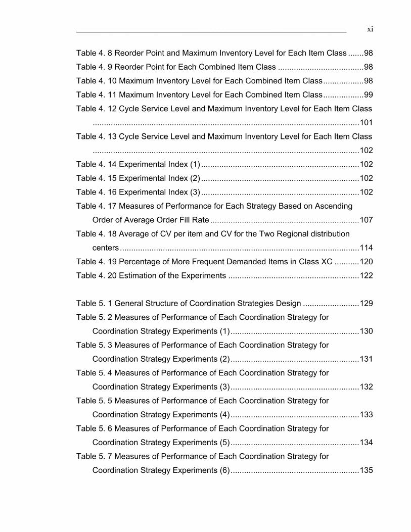
Table 4. 8 Reorder Point and Maximum Inventory Level for Each Item Class .......98
Table 4. 9 Reorder Point for Each Combined Item Class ......................................98
Table 4. 10 Maximum Inventory Level for Each Combined Item Class..................98
Table 4. 11 Maximum Inventory Level for Each Combined Item Class..................99
Table 4. 12 Cycle Service Level and Maximum Inventory Level for Each Item Class
......................................................................................................................101
Table 4. 13 Cycle Service Level and Maximum Inventory Level for Each Item Class
......................................................................................................................102
Table 4. 14 Experimental Index (1) ......................................................................102
Table 4. 15 Experimental Index (2) ......................................................................102
Table 4. 16 Experimental Index (3) ......................................................................102
Table 4. 17 Measures of Performance for Each Strategy Based on Ascending
Order of Average Order Fill Rate ..................................................................107
Table 4. 18 Average of CV per item and CV for the Two Regional distribution
centers ..........................................................................................................114
Table 4. 19 Percentage of More Frequent Demanded Items in Class XC ...........120
Table 4. 20 Estimation of the Experiments ..........................................................122
Table 5. 1 General Structure of Coordination Strategies Design .........................129
Table 5. 2 Measures of Performance of Each Coordination Strategy for
Coordination Strategy Experiments (1) .........................................................130
Table 5. 3 Measures of Performance of Each Coordination Strategy for
Coordination Strategy Experiments (2) .........................................................131
Table 5. 4 Measures of Performance of Each Coordination Strategy for
Coordination Strategy Experiments (3) .........................................................132
Table 5. 5 Measures of Performance of Each Coordination Strategy for
Coordination Strategy Experiments (4) .........................................................133
Table 5. 6 Measures of Performance of Each Coordination Strategy for
Coordination Strategy Experiments (5) .........................................................134
Table 5. 7 Measures of Performance of Each Coordination Strategy for
Coordination Strategy Experiments (6) .........................................................135

___________________________________________________________________
xii
Table 5. 8 Measures of Performance of Each Coordination Strategy for
Coordination Strategy Experiments (7) .........................................................136
Table 5. 9 Correlation Coefficient between Number of Pallets and Reduction in
Transportation Cost ......................................................................................146
Table 5. 10 Improving Order Fill Rate of the Four Selected Experiments ............150
Table 5. 11 Increasing Total Logistics Costs of the Four Selected Experiments .150
Table 6. 1 Percentage of Items in each Class for each Distribution Center .........163
Table 6. 2 Reorder Point and Maximum Inventory Level for Each Item Class .....167
Table 6. 3 General Structure of Coordination Strategies Design Using the New
ABC Classification ........................................................................................169
Table 6. 4 Measures of Performance for Each Coordination Strategy and the Base
Strategy Based on Ascending Order of Average Order Fill Rate ..................170
Table 6. 5 Measures of Performance for the Selected Strategies.......................173
Table 6. 6 Measures of Performance for the Selected Strategies Based on
Ascending Order of Average Order Fill Rate ................................................175
Table 6. 7 Average of Percentage of Item in Each Class.....................................178
Table 6. 8 Measures of Performance and Comparisons Results of the two
Experiments for RDC17................................................................................179
Table 6. 9 Comparisons of Measures of Performance of the two Experiments for
RDC17..........................................................................................................179
Table 6. 10 Residual Stock of the A-item in the two Classifications....................180
Table 7. 1 General Structure of Coordination Strategies Design Using a New ABC
Classification.................................................................................................185
Table 7. 2 Measures of Performance for Each Experiments Sorted in Descending
Order of the Total Logistics Cost ..................................................................186
Table 7. 3 Measures of Performance for Each Experiments Sorted in Ascending
Order of Total Logistics Cost ........................................................................188
Table 7. 4 Total Numbers of Tours and Shipped Quantity (Pallets) for Each
Selected Experiment.....................................................................................190

___________________________________________________________________
xiii
Table 7. 5 Measures of Performance for Selected Experiments Sorted in
Descending Order of Total Logistics Cost.....................................................192
Table 7. 6 Measures of Performance of Lower Bound Transportation Cost
Experiment....................................................................................................197

___________________________________________________________________
xiv
List of Figures
Figure 1. 1 The Supply Chain Process ....................................................................2
Figure 2. 1 Classification of Supply Chain Coordination ........................................15
Figure 3. 1 DOSIMIS-3, DLL and Other Tools Interaction......................................24
Figure 3. 2 Elements of DOSIMIS-3 Modules for Building Supply Chain Simulation
Model ..............................................................................................................28
Figure 3. 3 Elements of DOSIMIS-3 Modules for Building Warehouse Location ...29
Figure 3. 4 Elements of DOSIMIS-3 Modules for Building Distribution Center
Location ..........................................................................................................29
Figure 3. 5 Simulation Model Input Data Parameter Masks...................................35
Figure 3. 6 Units of Transportation.........................................................................46
Figure 3. 7 Flowchart of Order Fulfillment Control Activities at Warehouse and
Distribution Center Locations..........................................................................48
Figure 3. 8 A Real Distribution Supply Chain Network...........................................51
Figure 3. 9 Plants and Distribution Centers Location .............................................51
Figure 3. 10 Number of Item Types per Plant ........................................................53
Figure 3. 11 Number and Percentage of Replenished Items from each Warehouse
type to each Distribution Center......................................................................54
Figure 3. 12 Average Number of Order Lines per Distribution Center ...................55
Figure 3. 13 Number of Customers per Distribution Center ...................................56
Figure 3. 14 Aggregated Average Daily Demand...................................................57
Figure 3. 15 Percentage of each Probability Distribution of Demand.....................59
Figure 3. 16 Average of the Coefficient of Variation per Item for each Distribution
Center .............................................................................................................60
Figure 3. 17 DOSIMIS-3 Simulation Model Snapshot ............................................64
Figure 3.18 Flow Logical Processes of Consolidation Concept .............................69
Figure 3. 19 Mask Parameters for VMI and Consolidation Concepts.....................78

___________________________________________________________________
xv
Figure 3. 20 Flow of Logical Processes of Consolidation Concept under VMI Model
........................................................................................................................79
Figure 4. 1 ABC Classification for LDC1 ................................................................82
Figure 4. 2 ABC Classification for LDC5 ................................................................83
Figure 4. 3 ABC Classification for RDC15 .............................................................83
Figure 4. 4 ABC Classification for RDC19 .............................................................84
Figure 4. 5 Average Percentages of Items in each Class ......................................85
Figure 4. 6 XYZ Classification for LDC1 ................................................................87
Figure 4. 7 XYZ Classification for LDC5 ................................................................87
Figure 4. 8 XYZ Classification for RDC15..............................................................88
Figure 4. 9 XYZ Classification for RDC19..............................................................88
Figure 4. 10 Average Percentages of Items in each Class ....................................89
Figure 4. 11 Percentage of Items in each Class for each Distribution Center........90
Figure 4. 12 Average Percentages of Items in each Class ....................................91
Figure 4. 13 Measures of Performance for Each Strategy Based on Ascending
Order of Average Order Fill Rate ..................................................................107
Figure 4. 14 Percentage Increase of the Total Logistics Costs............................108
Figure 4. 15 Costs Categories Shares Regarding Logistics Costs for All Strategies
......................................................................................................................111
Figure 4. 16 Average Order Fill Rate of Selected Strategies for Each Distribution
Center ...........................................................................................................112
Figure 4. 17 Total Transportation Costs of Selected Strategies for Each Distribution
Center ...........................................................................................................112
Figure 4. 18 Total Inventory Holding Cost of Selected Strategies for Each
Distribution Center ........................................................................................113
Figure 4. 19 Order Fill Rate of Each Distribution Center for Each Strategy ........116
Figure 4. 20 Average Item Fill Rates of Each Combined Item Class (RDC3) ......117
Figure 4. 21 Average Item Fill Rate of Each Combined Item Class (RDC6) ........118
Figure 4. 22 Average Item Fill Rate of Each Combined Item Class (RDC15) ......118
Figure 4. 23 Average Item Fill Rate of Each Combined Item Class (RDC19) ......119
___________________________________________________________________
xvi
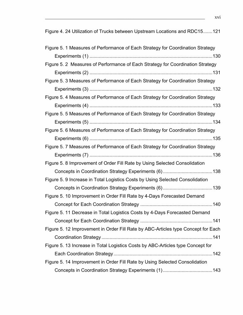
Figure 4. 24 Utilization of Trucks between Upstream Locations and RDC15.......121
Figure 5. 1 Measures of Performance of Each Strategy for Coordination Strategy
Experiments (1) ............................................................................................130
Figure 5. 2 Measures of Performance of Each Strategy for Coordination Strategy
Experiments (2) ............................................................................................131
Figure 5. 3 Measures of Performance of Each Strategy for Coordination Strategy
Experiments (3) ............................................................................................132
Figure 5. 4 Measures of Performance of Each Strategy for Coordination Strategy
Experiments (4) ............................................................................................133
Figure 5. 5 Measures of Performance of Each Strategy for Coordination Strategy
Experiments (5) ............................................................................................134
Figure 5. 6 Measures of Performance of Each Strategy for Coordination Strategy
Experiments (6) ............................................................................................135
Figure 5. 7 Measures of Performance of Each Strategy for Coordination Strategy
Experiments (7) ............................................................................................136
Figure 5. 8 Improvement of Order Fill Rate by Using Selected Consolidation
Concepts in Coordination Strategy Experiments (6) .....................................138
Figure 5. 9 Increase in Total Logistics Costs by Using Selected Consolidation
Concepts in Coordination Strategy Experiments (6) .....................................139
Figure 5. 10 Improvement in Order Fill Rate by 4-Days Forecasted Demand
Concept for Each Coordination Strategy ......................................................140
Figure 5. 11 Decrease in Total Logistics Costs by 4-Days Forecasted Demand
Concept for Each Coordination Strategy ......................................................141
Figure 5. 12 Improvement in Order Fill Rate by ABC-Articles type Concept for Each
Coordination Strategy ...................................................................................141
Figure 5. 13 Increase in Total Logistics Costs by ABC-Articles type Concept for
Each Coordination Strategy ..........................................................................142
Figure 5. 14 Improvement in Order Fill Rate by Using Selected Consolidation
Concepts in Coordination Strategy Experiments (1) .....................................143

___________________________________________________________________
xvii
Figure 5. 15 Increase in the Total Logistics Costs by Using Selected
Consolidation Concepts in Coordination Strategy Experiments (1) ..............144
Figure 5. 16 Real Curve and Fitted Curve of Transportation Cost ($) Function in
RDC9............................................................................................................146
Figure 5. 17 Real Curve and Fitted Curve of Transportation Cost ($) Function in
RDC13..........................................................................................................147
Figure 5. 18 Real Curve and Fitted Curve of Transportation Cost ($) Function in
RDC19..........................................................................................................147
Figure 5. 19 Reduction in Transportation Cost.....................................................148
Figure 5. 20 Relationship between the Number of Pallets and the Truck Utilization
......................................................................................................................148
Figure 5. 21 Percentage of Increase in the Average Residual Stock by Each
Consolidation Concept in RDC17 [A-Item]....................................................152
Figure 5. 22 Percentage of Increase in the Average Residual Stock by Each
Consolidation Concept in RDC19 [A-Item]....................................................152
Figure 5. 23 Residual Stock and Reorder Point of A-Item Using 4-Days Forecasted
Demand Consolidation Concept in RDC19...................................................153
Figure 5. 24 Residual Stock of ZA Item Using (Z-Articles) Consolidation Concept in
RDC19..........................................................................................................154
Figure 5. 25 Residual Stock of ZA Item Using (A-Articles) Consolidation Concept in
RDC19..........................................................................................................155
Figure 5. 26 Comparison of Increasing Average Residual Stock (%) of ZA-Item in
Two Distribution Centers (RDC17 & RDC19) ...............................................156
Figure 5. 27 Average Percentage of A-Item from Suppliers (Warehouses) to
Distribution Centers ......................................................................................157
Figure 5. 28 Truck Utilization between Upstream Locations and RDC15 ............158
Figure 6. 1 ABC New Classification for LDC1......................................................161
Figure 6. 2 ABC New Classification for LDC5......................................................162
Figure 6. 3 ABC New Classification for RDC15 ...................................................162
Figure 6. 4 ABC New Classification for RDC19 ...................................................163

___________________________________________________________________
xviii
Figure 6. 5 Percentage of Items in A Class for each Distribution Center in Two
Classifications...............................................................................................164
Figure 6. 6 Percentage of Items in B Class for each Distribution Center in the two
Classifications...............................................................................................165
Figure 6. 7 Percentage of Items in C Class for each Distribution Center in the two
Classifications...............................................................................................165
Figure 6. 8 Average Percentages of Items in each Class for the two Classifications
......................................................................................................................166
Figure 6. 9 Measures of Performance for Each Strategy Based on Ascending
Order of Average Order Fill Rate ..................................................................171
Figure 6. 10 Percentage of Improved Order Fill Rate by each Coordination Strategy
......................................................................................................................172
Figure 6. 11 Percentage of Increased Total Logistics Costs by Each Coordination
Strategy ........................................................................................................172
Figure 6. 12 Measures of Performance for the Selected Strategies Based on
Ascending Order of Average Order Fill Rate ................................................175
Figure 6. 13 Percentage of Improved Order Fill Rate by the Selected Coordination
Strategy ........................................................................................................176
Figure 6. 14 Percentage of Increased Total Logistics Costs by the Selected
Coordination Strategy ...................................................................................176
Figure 6. 15 Number of Replenishments for Each Distribution Center using the two
Different Consolidation Concepts .................................................................177
Figure 7. 1 Total Logistics Costs and Transportation Cost for Each Experiment .186
Figure 7. 2 Total Average Inventory Cost for Each Experiment ...........................187
Figure 7. 3 Percentage of Increasing Total Logistics Costs by Each Experiment 189
Figure 7. 4 Percentage of Increasing Total Transportation Cost by Each
Experiment....................................................................................................189
Figure 7. 5 Total Number of Tours and Shipped Quantities (Pallets) for Each
Selected Experiment.....................................................................................191

___________________________________________________________________
xix
Figure 7. 6 Total Logistics Costs and Transportation Cost for the Selected
Experiments..................................................................................................193
Figure 7. 7 Total Average Inventory Cost for the Selected Experiments..............193
Figure 7. 8 Percentage of Decreased Total Logistics Costs for the Selected
Experiments..................................................................................................194
Figure 7. 9 Truck Utilization between Upstream Locations and Downstream
Locations for UCS-V-Expt Strategy ..............................................................195
Figure 7. 10 Truck Utilization between Upstream Locations and Downstream
Locations for CS-V-4D-Expt 9 Strategy ........................................................196

Chapter 1. Introduction 1
1. Introduction
1.1. Definition of Supply Chain
Supply chain management (SCM) has been recently presented to address the
coordination and integration of organizational functions, ranging from the supply
and receipt of raw materials throughout the manufacturing stages, to the
distribution and delivery of final products to the end customer. Its application
demonstrates that this idea enables companies to achieve higher quality products,
better customer service, and lower inventory and transportation costs. In order to
achieve high system performance, supply chain functions (processes) must
operate in an integrated and coordinated manner.
The SCM literatures offer many definitions and frameworks of a supply chain
[MDK01], [Tan01], [LGC05], [SB06]. Beamon [Bea98] defined a supply chain as an
integrated manufacturing process herein raw materials are converted into final
products and then delivered to customers. At its highest level, a supply chain is
comprised of two basic and integrated processes: (1) Production Planning and
Inventory Control Process and (2) Distribution and Logistics Process. These
processes are illustrated below in Figure 1.

Chapter 1. Introduction 2
Figure 1. 1 The Supply Chain Process
According to Simchi-Levi et al. [SKS03], a supply chain is “a set of approaches
utilized to efficiently integrate suppliers, manufactures, warehouses, and stores, so
that merchandise is produced and distributed at the right quantities, to right
locations, and at the right time, in order to minimize systemwide costs while
satisfying service level requirements”.
As stated by Ballou [Bal04], “The supply chain encompasses all activities
associated with the flow and transformation of goods from the raw materials stage
(extraction), through to the end user as well as the associated information flows.
Materials and information flow both up and down the supply chain. Supply chain
management (SCM) is the integration of these activities, through improved supply
chain relationships, to achieve a sustainable competitive advantage”.
Nilsson [Nil6] summarized the new trends in the SCM and logistics as discusses by
Waters [Wat03]. There are 12 different trends in logistics today. These are:
• Improving communications. Better communication within the supply chain
with new technologies such as Electronic Data Interchange (EDI).

Chapter 1. Introduction 3
• Improving customer service. Making logistics cost as low as possible and
increasing high service levels at low costs.
• Globalization. Firms operations are becoming more and more international
when trade and competition are rising.
• Reduced number of suppliers. The number of suppliers is reduced and long
term relationships are created.
• Concentration of ownership. When the companies experience economics of
scale the competition is concentrated to fewer players on the market.
• Outsourcing. More and more logistics operations are outsourced to
specialized companies.
• Postponement. The movement of almost-finished goods into the distribution
system and delays of final modifications.
• Cross-docking. When incoming goods are shipped again without being
stored at the warehouse.
• Direct delivery. Direct shipping from manufacturer to final customer.
• Other stock reduction methods. Newer methods such as Just-in-Time and
Vendor Managed Inventories.
• Increasing environmental concerns. The movement towards ‘greener’
practices among logistics operations.
• More collaboration along the supply chain. Aiming towards the same
objectives and no internal competition within the supply chain.
This thesis is based on three of the logistics trends outlined above; improving
customer service, cross-docking and other stock reduction methods. Procuring
several items from upstream locations to downstream locations in supply chains
requires well functioning coordination regarding transportation and inventory
decisions, and therefore, this thesis deals mainly with the common problems of
transportation and inventory coordination.

Chapter 1. Introduction 4
1.2. Coordination in Supply Chains
Supply chain consists of many systems including manufacturing, storage,
transportation, and retail systems. Managing of any one these systems involves a
series of complex trade-offs. Additionally, these systems are connected and hence
the outputs from one system within the supply chain are the inputs to the next
system. For example the outputs from the production system may be the inputs to
a transportation or inventory system. Therefore the various systems need some
kind of coordination to operate effectively.
Coordinating supply chain activities maximises the supply chain performance
[SKS03]. Supply chain coordination improves if all the stages of the chain take
actions that altogether increase total supply chain profits. Supply chain
coordination requires each stage of the supply chain to take into account the
impact its actions have on other stages.
A coordination mechanism is a set of methods used to manage the interactions
between multiple supply chain tiers. To increase the high-performance of supply
chain, an organization should select the appropriate coordination mechanism
[XB06]. A lack of coordination occurs either because different stages of the supply
chain have objectives that may conflict, or because information moving between
different stages may have been distorted [CM04].
The management of the entire supply chain has become possible in the recent
years due to new developments in the technology of information systems. But still it
is obviously much more difficult than dealing with each of the traditional production,
transportation and inventory decision problems separately.
In spite of the difficulty in managing a supply chain, the coordination of inventory
polices and transportation strategies are the key terms for an efficient management
of the supply chain. Transportation strategies include the application of different
types of shipment consolidation (freight consolidation) policies. The consolidation
policy coordinates the shipping of different item orders for the same destination,

Chapter 1. Introduction 5
and this can lead to a reduction in transportation costs. Higginson and Bookbinder
[HB94] present a simple discrete-event simulation model to distinguish between
three types of consolidation policies: the time policy, the quantity policy and the
time-and-quantity policy. The time policy dispatches orders at a scheduling
shipping date. The quantity policy dispatches orders when a fixed consolidated
quantity is reached. The time-and-quantity policy is a mixed policy of the time and
the quantity policies. Instead of using simulation, Higginson and Bookbinder [HB95]
use a Markov chain model to determine the optimal consolidation policy given as
an (s,S) continuous review inventory policy generating shipment orders, where s is
reorder point and S is order-up-to level. In this thesis, a new shipment
consolidation concept (quantity policy) based on item classification approach is
developed and a discrete-event simulation model to test this concept for effective
coordination is developed.
With recent advances in communication and advanced information technology,
companies have better chance for substantial savings in the total logistics costs by
coordinating and integrating the different stages in the supply chain. Clearly,
companies realize that the sharing of information through the supply chain is
beneficial. As is already known, to coordinate and integrate the supply chain
effectively, the information must be available and shared. Several information
technologies (IT) have been developed recently in order to facilitate this. Electronic
data interchange (EDI), the Internet, and Web sites are some of these
technologies. By applying these technologies, many new supply chain initiatives,
such as Vendor Managed Inventory (VMI), are constructed and implemented.
VMI is a coordination mechanism in which the upstream member of the supply
chain manages the inventory level and the appropriate inventory policies on its
downstream member of the supply chain. In VMI, one can optimize the entire
system performance by coordinating inventory and distribution. As suggested by
Silver et al. [SPP98], the VMI is one of the new future developments in supply
chain initiatives that could be expanded as the next competitive source of supply
chain coordination. Therefore in this thesis, the VMI is implemented for a real life

Chapter 1. Introduction 6
supply chain to see the benefits of using this approach on the coordination of
supply chains and how this approach can be incorporated effectively to develop a
new coordination strategy. Furthermore, the most important requirement for an
effective coordination, especially for a VMI, is advance demand information.
Contemporary research has been conducted on how a supplier can make use of
customer demand information for better demand forecasts and inventory control
policies [GKT96], [CF00], [LST00], [AF98]. In industry, there has been great
interest expressed in the concept of a supplier making use of downstream demand
information to coordinate the replenishments or shipments [CL02]. Here,
coordinating the shipment is the practice used by the supplier in order to make the
timing and quantity of replenishment decisions for the retailers, the advance
demand information being provided by the retailers [CL02]. In this thesis, a new
shipment consolidation concept (quantity policy) that uses the advance demand
information technology for consolidating shipments is developed. For effective
coordination between the inventory and transportation decisions and for optimizing
of the real supply chain, this concept is linked to VMI programs.
In reality supply chains are complex and consist of numerous companies. The
companies have different complex network structures. These companies realize
that great savings of the total logistics cost can be obtained by effective designing
of the supply chain network and distribution strategies.

Chapter 1. Introduction 7
1.3. Motivation
This thesis was motivated by a real life food supply chain company located in a
European country. This company wanted to optimize its supply chain network and
the distribution strategies.
The supply chain distribution network model that should be analyzed is typically
complex; it considers many strategies to be changed over time. The mathematical
optimization techniques have some limitations as they deal only with static models.
However, simulation based tools which take into account the dynamics of the
system are capable of characterizing system performance for a given design.
In this research, the distribution network simulation model was created by using
DOSIMIS-3, with support of C++ program it was specifically developed for the
supply chain simulation purpose. Some other tools were customized for use with
this particular model. The validation of the simulation model has been done by
comparing the simulated results with the historical data obtained from the logistic
department of the company. Therefore, in this thesis, the simulation model is
extended to include and to implement all aspects of the new prescriptive of supply
chains that have been discussed. Another motivation is the availability of significant
amount of historic data (more variations and dynamic) from the company’s ERP
system which has been used to conduct all the simulation studies in this thesis.
1.4. Outline of the Thesis
The thesis consists of eight chapters. These chapters are organized as follows:
Chapter 1 gives a brief introduction on the supply chain and supply chain
coordination. Chapter 2 gives a survey of the existing literatures in the fields to
overview the variations of the integrated problems in supply chains and supply
chain simulation. In this chapter, the goals of the dissertation are presented.
Chapter 3 deals with simulation modeling of supply chains. The chapter on

Chapter 1. Introduction 8
simulation modeling of supply chains gives an overview of the various activities
involved in the supply chain. This chapter discusses in detail the description of the
developed simulation model. The chapter also discusses the procedure and tools
adopted for carrying out the simulation. The various features of the simulation
model including the performance measures are also explained. The real life
problem is presented and explained in this chapter. Extend studies on the real life
case study are also described, the logic methodology and the steps of the two new
consolidation concepts are also explained. An in depth description of the
implementation of the coordination strategies and VMI concept using the
developed simulation model is also given in this chapter.
Chapter 4 deals with the designing and the conducting of the uncoordinated
strategies based on the item classification approaches. Two item classification
approaches (ABC & XYZ) are presented in this chapter. The detailed description of
the designing, resulting, and analysis of the experiments are also presented in this
chapter. The main measures of performance used in this thesis are also described
in this chapter. In Chapter 5, description of how to design and conduct the
coordination strategies using the two new consolidation approaches is presented.
All the results and analysis of the results of the coordination experiments are also
presented in this chapter. Chapter 6 presents the optimization of coordination
strategies by using a newly developed item classification. This new item
classification is explained in this chapter. The new coordination strategies
developed based on this new classification are also described. Results and
analysis of these new strategies are summarized and illustrated in this chapter. In
Chapter 7, the use of the Vendor-Managed Inventory (VMI) programs for
constructing optimal coordination strategies is described and presented.
Comparative studies are conducted and exhibited in this chapter. Finally, Chapter
8 summarizes the results and conclusions with some recommendations which
would be useful for future studies.

Chapter 2. Literature Review 9
2. Literature Review
A large body of literature exists on the coordination and integrated supply chains.
This chapter gives an outline of the literature reviewed for the purposes of this
work. In Section 2.1, a review of the literature on supply chain coordination is
given. Section 2.2 discusses supply chain simulation frameworks that have been
proposed in the past. Section 2.3 deals with goals of the dissertation.
2.1. Overview of various approaches on the coordination and integrated problems in supply chains
Several approaches can be found in the literature, which provide models to
coordinate at least two stages of the supply chain and which can detect new
opportunities that may exist for improving the efficiency of the supply chain.
Beginning with Clark and Scarf in 1960 [CS60], many researchers have considered
multi-echelon distribution-inventory problems. This problem considers a central
plant (warehouse) that allocates a product (or products) to a number of customers
with the objective of minimizing overall total costs including holding cost and
transportation cost [AF90], [AF90], [FZ84]. The decision variables which have been
considered in the problem are shipment sizes and delivery routes.
A large amount of researches has been conducted on the inventory-distribution
coordination [DB87], [Cha93]. Anily and Federgruen [AF90] have studied a model
integrating inventory control and transportation planning decisions motivated by the
trade-off between the size and the frequency of delivery. They have considered a
single-warehouse and multi-retailer scenario where inventory would be kept only at
the retailers that face constant demand. The model determines the replenishment
policy at the warehouse and the distribution schedule for each retailer so that the

Chapter 2. Literature Review 10
total inventory and distribution costs are minimized. They have presented heuristic
procedures to find upper and lower bounds on the optimal solution value.
Bhatnagar et al. [BCG93] classified the issue of coordination in organizations in to
two problems. The first problem is the General Coordination problem (coordination
between functions) and the second problem is the Multi-Plant Coordination
problem (coordination within the same function at different echelons in an
organization). They study the Multi-Plant Coordination problem. The authors have
presented a good categorization and some literature review for the general
coordination problem. Within this problem they have distinguished three categories
that represent the integration of decision making pertaining to: (1) supply and
production planning, (2) production and distribution planning, and (3) inventory and
distribution planning.
Thomas and Griffin [TG96] defined three categories of the operational coordination
of the supply chain management. These three categories are: (1) Buyer-vendor
coordination, (2) Production-distribution coordination, (3) Inventory-distribution
coordination. Also they have made a review study on the supply chain coordination
and list some topics for future work.
Viswanathan and Mathur [VM97] studied the same problem as Anily and
Federgruen [AF90] with the generalization of multiple products in the system. They
have developed a heuristic based on a joint replenishment problem to obtain a
stationary nested joint replenishment policy (SNJRP). They have considered
vehicles with limited capacity and present computational results comparing the
performance of the proposed heuristic with the heuristics proposed by Anily and
Federgruen [AF90], for the case of a single product. Their results show that the
SNJRP policy performs better in the majority of cases in terms of cost. The authors
have reported that no other heuristic was known to handle multiple products.
Therefore, a comparison was not possible for problems that consider more than
one product in the system.
Chapter 2. Literature Review 11
Sarmiento and Nagi [SN99] presented a review on the integrated analysis of
production-distribution systems, and have identified important areas where further
research would be needed. They have suggested that further research in the
Inventory/Distribution problem could take into consideration more complex
networks for analysis. Algorithms that explicitly consider the location of several
customers and depots, as well as the routing of vehicles and inventory levels
setting are needed for more complete dynamic scenarios. While optimal solutions
are very difficult to obtain, heuristic procedures could be developed to obtain
approximate solutions for this complex problem. Validation methods would also be
required. Research is also needed for the explicit consideration of multiple
products in the system. The analysis of different instances of the
Inventory/Distribution problem under stochastic demand considerations is still a
largely open research area. Further research is also needed for Inventory/
Distribution scenarios that would acknowledge the existence of emergency
shipments, and would consider a constrained transportation system.
Morales [Mor00] studied a class of optimization models, which would integrate both
transportation and inventory decisions, to search for opportunities for improving the
logistics distribution network. He considered a set of plants and a set of
warehouses to deliver the demand to the customers, he proposed a class of
greedy heuristics, and showed that significant improvements could be made by
using the result of the greedy heuristic as the starting point of two local exchange
procedures, yielding very nearly optimal solutions for problems with many
customers.
Yang [Yan00] considered a single- warehouse multiple-retailer (SWMR) system.
His work is one of the first to examine the relative impact of various policies and
environmental factors on the performance of an SWMR system. He suggested
three important environmental factors and four policies that may affect the
performance of an SWMR system. The three environmental factors are: the
number of stores, order processing time and demand variability. The four policies
are: the warehouse location, vehicle-scheduling rule, inventory rule and order size.

Chapter 2. Literature Review 12
He has developed a simulation model of an SWMR system using SLAM II. The
simulation result shows that the number of stores, demand variability, order size
and order processing time have a much larger impact on the performance than the
inventory and vehicle-scheduling rules. This paper also provides some suggestions
for future research. The environmental factors, for instance, have demonstrated a
much larger impact on the performance than the inventory and vehicle-scheduling
rules. Future research should therefore examine the impact of the environmental
factors in greater details, such as the impact of variable order processing times.
Another possible area for future research is a detailed comparison between the
Continuous Review and Periodic Review policies.
Min and Zhou [MZ02] offered an effort to help firms capture the synergy of inter-
functional and inter-organizational integration and coordination across the supply
chain and subsequently make better supply chain decisions. This effort is based on
the prior supply chain modelling efforts. They present the models that attempt to
integrate different functions of the supply chain as the supply chain models. Such
models deal with the multi-functional problems of location/routing,
production/distribution, location/inventory control, inventory control/transportation,
and supplier selection/ inventory control.
Liu [Liu03] concluded that most of the integrated production-distribution models
consider transportation elements as a fixed cost, and no routing or other
transportation capacity issues are involved. In other words, these models consider
only the demand allocation element in distribution, and make decision based only
on how much product has to be transported from production plant to customers.
There is no decision on how the transportation function is carried out. Most of
these models, with few exceptions, do not consider how these quantities can be
transferred by transporters with their capacity, speed, and availability (constrained
time to operate). Based on that Liu [Liu03] proposed and evaluated the
effectiveness of a two-phase solution methodology for solving the integrated
production, inventory and distribution problem (PIDP) where the transporters
routing must be optimized together with the production lot sizes and the inventory

Chapter 2. Literature Review 13
policies. The phase I model, a PIDP with direct shipment, is solved as a mixed-
integer programming problem subject to all the constraints in the original model,
except that the transporters routings are restricted to direct shipment. To handle
the potential inefficiency of the direct shipment, Phase II applies a heuristic
procedure (the Load Consolidation (LC) algorithm) to solve an associated
consolidation problem. The associated delivery consolidation problem is formulated
as a capacitated transportation problem with additional constraints. In this
capacitated transportation problem, transporters in the heterogeneous fleet are
allowed to make multiple trips per period. His study on this problem enriches the
existing literature of Vehicle Routing Problem (VRP), and the proposed LC
algorithm provides an alternative to solve complicated real life distribution problems
with a heterogeneous fleet that allows multiple trips per transporters. There are
several potential extensions from this work. Firstly, from a practical point of view,
models that allow the distribution centre (DC) demands to be random variables and
that some DC’s to be used as transshipment points could be of great value to real
world needs. Secondly, there have been a vast amount of research results
available for capacitated vehicle routing. A comparative study of the LC algorithm
used in Phase II of this study with existing heuristics in the literature results has a
potential to further improve the solution quality of the approaches to the integrated
production, inventory and distribution routing problems. Finally, he assumes that
each plant owns a fixed fleet of heterogeneous transporters, and that the
transporters owned by one plant do not travel to other plants.
Mason et al. [MRF03] examined the total cost benefit that could be achieved by
suppliers and warehouses through the increased global visibility provided by an
integrated system. They developed a discrete event simulation model of a multi-
product supply chain to examine the potential benefits to be gained from global
inventory visibility, trailer yard dispatching and sequencing techniques. From the
simulation results they showed that queue dispatching rules significantly affect total
cost, by assigning the sequence of loading and unloading trucks. Queue
dispatching rules also aid cross-docking, which significantly reduces holding and

Chapter 2. Literature Review 14
back-ordering costs. They suggested for future research that in order to quantify
operational improvements resulting from the implementation of an integrated
system. It would be necessary to establish a set of metrics to ensure that overall
supply chain costs are reduced, rather than simply optimizing the various
components of the supply chain individually. Potential issues to be considered
include the coordination of replenishment when a single vendor supplies multiple
SKUs (Stock Keeping Unit), so that full-truckload trucking can be utilized. When a
pull system is implemented, initially ordered quantities are smaller due to existing
safety stock. This may result in less than full-truckload trucking. However,
assuming that demand does not decrease, as soon as the system exhausts the
safety stock, the system should reach equilibrium and reverts back to full-truckload
trucking.
Another line of research in coordination of supply chain is the joint replenishment
or coordinated replenishment problem. The Joint Replenishment Problem (JRP) is
a research topic in the area of multi-item inventory problems that has been
generating interest for many years as it is a common real-world problem that
occurs in different situations, for instance, when a group of items are replenished
from the same supplier or when a product after manufacturing is packaged in
different quantities. Goyal [Goy73], [Goy74] gives a more detailed definitions and
descriptions of the problem.
Goyal and Satir [GS89] presented an early review of all models, starting from a
simple deterministic problem. In the joint replenishment literature, two types of
control policy were presented. These are: the continuous review can-order policy
),,( iii Scs and the periodic review order-up-to policy ),( ii SR . In the continuous can-
order policy ),,( iii Scs , when the inventory position of an item i reaches the must-
order point is , replenishment is triggered as to raise the item’s inventory position to
order-up-to level iS . Meanwhile, any other item in the group with an inventory
position at or below its can-order point ic is included in the replenishment as to
raise the inventory position up to iS [LY00], [FGT84]. In the periodic review

Chapter 2. Literature Review 15
policy ),( ii SR , the inventory position of item i is inspected with intervals iR and the
review moments are coordinated in order to consolidate orders of individual items
[VM97].
Silver et al. [SPP98] explained the cost savings that can be achieved by
coordinating the replenishment of several items. Sombat et al. [SRE05], Chen and
Chen [CC05], and Nilsson [Nil06] give a more detailed information on the JRP and
associated issues. As can be seen from literature, due to the difficulty of
coordination problems, most of the models proposed are analytical models which
consider simple supply chain networks, therefore, they limit more investigations on
the supply chain coordination. Rather simulation models can be used to handle
and analyse complex problems. Figure 2.1 summarizes the classification of supply
chain coordination as presented in the lite7rature.
Figure 2. 1 Classification of Supply Chain Coordination
The dashed boxes in the above figure indicate the points of focus of this thesis.
Integrated Supply Chain Modeling
Supplier Selection/Inventory Control
Production/Inventory
Location/Inventory Control
Inventory Control/Transportation
Supply and Production or Buyer-vendor Coordination
Production and DistributionCoordination
Inventory and DistributionCoordination
Distribution –InventoryModels
Inventory –Distribution–InventoryModels
Production –Inventory –Distribution–InventoryModels
Thomas and Griffin 1996)
Samiento and Nagi (1999)
Min and Zhou (2002)
Coordination in an Organisation
General CoordinationProblem (function)
Multi –plant Coordination(same function at different echelons)
Bhatnagar et al.(1993)
Coordination in an Organisation
General CoordinationProblem (function)
Multi –plant Coordination(same function at different echelons)
Bhatnagar et al.(1993)

Chapter 2. Literature Review 16
2.2. Overview of the supply Chain Simulation
There are extensive literatures available on the analysis of supply chain
coordination. Two of the most common ways of analyzing a supply chain are
simulation and analytical modeling. The literature on the analytical modeling is
presented in the previous section. This section summarizes some of the significant
research on supply chain simulation.
Cachon and Fisher [CF97] examined forecasting and inventory management under
VMI for Campbell's Soup. Using simulations of their ordering rules, they have found
that both retailers’ and manufacturers’ inventories could be reduced while
improving service. They did not consider cases with limited manufacturing capacity
and issues related to allocating inventory across retailers.
Vendor-managed inventory (VMI) is one of the most widely discussed partnering
initiatives for improving multi-firm supply chain efficiency. Waller et al. [WJD99]
introduced a simulation model that examines VMI quantitatively in order to
understand the effect of key variables. Bhaskaran [Bha98] performed an analysis
of supply chain instability for an automobile industry. In this study, it is shown how
supply chains can be analyzed for continuous improvement opportunities using
simulation. For building the simulation model, automobile supply chain simulation
software originally developed to GM’s specifications was used. This supply chain
simulation software could be used to study the impact of many production control
and material management policies on important measures such as inventory
levels, forecast stability, and material shortages.
In supply chain modeling, effort is made to consider the effect of policies on the
performance of the supply chain. The effects of policies are tested either
analytically or through simulation. In the case of simulation for supply chains, effort
involved in building the supply chain simulation model can be reduced to a great
extent if the models can be built hierarchically from existing modules. Eliter et al.
[ESP98] worked on the concept of Agent Programs. An agent consists of a body of

Chapter 2. Literature Review 17
software code that supports a well-defined application programmer interface and a
semantic wrapper that contains a wealth of information. As part of the work, the
team developed agents for various functions of supply chain management
systems. A simulation model of a supply chain application based on agents was
built using commercial software such as Microsoft Access and ESRI’s MapObject.
Swaminathan et al. [SSS98] described a supply chain modeling framework that
can be used for constructing supply chain simulation models. They develop
software components for representing various types of supply chain agents such
as retailers, manufacturers and transporters. The authors divide the set of
elements in their supply chain library into two categories: Structural Elements and
Control Elements. Structural elements correspond to agents (eg manufacturer
agents, transportation agents) and control elements correspond to the control
policies.
Bagchi et al. [BBE98] discussed the IBM’s Supply Chain Simulator. Supply chain
simulation involves the simulation of both inter-facility and intra-facility operations.
For example, a supply chain simulation tool may model MRP processes, planning
and scheduling, capital acquisition, labour and other resources, transportation
policies, stocking policies, etc. Bagchi et al. [BBE98] indicated that the key to the
usefulness of a supply chain simulator is the ability to translate the simulation
information into costs and financial reports. This is typically achieved through the
use of activity base costing models.
Jain et al. [JWC01] observed that the level of details included in the development
of a simulation model should be appropriate to the objective of the study. They
concluded that inclusion of more detail than necessary can easily lead to too large
an effort for the objective at hand and the effort not being approved by the parent
organization. As part of the work, the authors developed a high level supply chain
simulation model using a general-purpose simulation model. Their justification for
using general-purpose simulation software instead of a commercially available
supply chain simulation tool was that general-purpose simulation software lets the

Chapter 2. Literature Review 18
user select the desired level of abstraction. IBM Supply Chain Simulator is one of
the commercially available packages for simulating supply chains.
Díaz and Buxmann [DB03] examined how the benefits of Supply Chain
Management, as reported by the literature and widely accepted, can simulatively
be proven. They presented selected results of a survey conducted on the
European automotive industry, which show an evident needed for transparency, in
terms of the quantification of the added-value of Supply Chain Management. For
this purpose an XML-based prototype for modeling and simulating cooperative
scenarios in supply chains is introduced, and illustrated its flexible architecture and
the interaction between modeled scenarios and optimization routines through XML
(Extensible Markup Language) interfaces. In the context of this prototype the
authors describe a simulation scenario in which the transportation activities in a
supply chain are modeled and planned.
Chu [Chu03] provided a comprehensive listing of simulation studies to summarize
their findings and to identify future research. He classified the simulation studies on
supply chains based on its major focus. Referring to his classification and
suggestions for future research, the developed simulation model in this thesis can
be classified as being a new simulation study to an industry, and new
enhancement strategies are to be tested and combined.
Schwarz et al. [SJX04] presented a review study on a class of supply chain
management problems which is called Integration or Joint transportation-and-
Inventory Problem (JTIP). They carried out a survey of 49 contemporary papers on
this problem and outlined problems that deserve further research and possible
ways to solve them. Based on their suggestion, this thesis considers two of these:
Multi-Product JTIP and Multi-Depot JTIP.
Terzi and Cavalieri [TC04] presented a comprehensive review made on more than
80 articles, the main purpose being to ascertain which general objectives
simulation is generally called to solve and which paradigms and simulation tools

Chapter 2. Literature Review 19
are most suitable. Useful prescriptions, both for practitioners and researchers, on
the applicability of simulation to decision-making processes within the supply chain
context were also derived.
By providing a systematic quantitative and objective evaluation of the outcomes
resulting from different possible planning scenarios, from demand planning to
transportation and distribution planning, simulation techniques can make
companies more aware of the benefits coming out from integrated and co-
operating strategies with their upstream/downstream locations rather than following
myopically an antagonistic behavior with them [TC04].
Regarding the above literature, few papers considered the coordination strategies
in supply chains using simulation models [Bea98], [TG96]. Therefore, this work
represents one of the new applications that uses simulation to model the
coordination strategies in the supply chains.
2.3. Goals of the Dissertation
Regarding to the significant and vast literature on the supply chain coordination
problems, this dissertation is designed to achieve some goals. These goals are:
• To study the optimization of distribution strategies, which integrate both
transportation and inventory decisions, to search for opportunities for
optimizing the supply chain performance
• To build a supply chain simulation model using a discrete-event simulation
tool for real life problems
• To use multi-item classification approaches for designing uncoordinated
distribution strategies
• To develop new shipment consolidation concepts for constructing new
coordination distribution strategies
• To develop new criteria for an item classification concept to be used for
designing an efficient coordination distribution strategy

Chapter 2. Literature Review 20
• To apply new initiatives and technologies in supply chain coordination
• To conduct more statistical tests for analysing the real life input data
• To interpret the problems resulting from the coordination strategies
• To estimate multi-criteria for evaluating the performance measures of supply
chains
• To conclude new findings and to suggest new trends for further work

Chapter 3. A real Life Case Study 21
3. Modeling Coordination Strategies in Supply Chains Using Simulation: A real-Life Case Study
3.1. Introduction
Supply chain management (SCM) is the management of the flow of
products/goods, services, and information from a supplier stage to the end-
customer stage. It is a complex process because of the level of uncertainty at each
stage of the supply chain. The main objective of problem-solving methods in
Supply Chain Management is to reduce uncertainties. Sources of uncertainty are,
e.g., the forecast horizon, input data, administrative and decision processes, and
inherent uncertainties [VBW98].
One major obstacle in creating a seamless supply chain is uncertainty. In order to
deal with this issue, managers must identify and understand the causes of
uncertainty and know how it affects other activities up and down the supply chain.
This helps them to formulate ways to reduce or eliminate it. Currently, tools for
understanding uncertainty are limited to traditional mathematical formulas that do
not account for variability. However, simulation is one of the best means for
analyzing supply chains because of its capability for handling variability.
Companies can use simulation to see how effective and costly an innovative
inventory system, such as just-in-time, would be in their own environment without
having to implement the system physically [SP00].
A supply chain is a network of facilities that performs the functions of procurement
of materials, transformation of these materials into intermediate and finished
products, and the distribution of these finished products to customers. A typical
supply chain may consist of many participants, such as suppliers, manufacturers,
distributors, retailers and the end customer. Each participant in the supply chain
has his own set of objectives. Due to its inherent complexity, analytical modeling of

Chapter 3. A real Life Case Study 22
supply chains becomes difficult. Moreover, a typical supply chain faces uncertainty
in many of its activities, for example, in the supply of raw materials from the
suppliers. Under such complex and uncertain situations, simulation becomes the
best alternative for analysis [Pun02].
In recent years, operation research models have put more emphasis on modeling
and analyzing multi-echelon distribution systems. Though SCM is relatively new,
the idea of coordination is not. Thomas and Griffin [TG96] presented an extensive
review on coordination of two or more stages of a supply chain and models
appropriate for modeling the supply chains.
The main drawback of most analytical models is the fact that numerous constraints
have to be satisfied before results can be applied in practice. Most models only
take a few variables into account, for example, inventory and running out of stock,
and ignore other cost, such as, order processing, handling and transportation.
Furthermore, these models neglect capacity restrictions [VBB00].
Due to the complexity of integrated problems, most of the models proposed in the
literature are static in nature and consider simple logistics distribution network.
Therefore, they do not allow more investigations on the coordination of
transportation and inventory decisions. Computer simulation is an especially
effective tool to help investigate and analyze complex problems. Because it can be
applied to operational problems that are too difficult to model and solve analytically
[TC04]. Moreover, mathematical models require too many simplifications and
assumptions to model coordination strategies in realistic supply chain problems.
Discrete event simulation permits complex logistics systems to be modeled more
realistically. This thesis therefore reports the findings of a vast investigation into the
discrete-event modeling and simulation of alternative designs and distribution
strategies for a supply chain of a food industry company.

Chapter 3. A real Life Case Study 23
3.2. Simulation Model Description
General-purpose discrete event simulation software cannot be directly used for
simulating supply chains. The simulation modules provided in the software should
be combined or modified to represent the activities typical to supply chains
[Pun02]. Based on this idea, a simulation tool is constructed. The simulation tool is
a discrete event model, developed based on the combining of the event-scheduling
and activity-scanning approaches [BCN03]. The model was created using
DOSIMIS-3, with support of a C++ program (DLL). It was developed specifically for
the supply chain simulation purpose. Some other tools were customized for the use
with this particular model. The database tools used in this model interface readily
with widely available application programs, such as Microsoft Excel, Access and
Visual Basic for Applications (VBA), to assist in scrutinizing the data.
DOSIMIS-3 is a discrete event simulation tool developed by
SimulationsDienstleistungsZentrum GmbH. It is an interactive using objects and
graphical working with Windows 95/98/NT/XP. The package is modular-oriented.
The simulator works event-discrete and allows simulation of time-discrete material
flow systems. A simulated production process can be developed graphically on the
screen with no special knowledge in the area of computing necessary. Standard
elements, such as sources, sinks, work stations, storages, vehicles etc., which in
their structure represent essential modules from the logistics field, allow a rational
layout by means of a menu-controlled user interface. Modules with several
entrances and exits deploy an intelligence over which local strategies, such as
FIFO, minimal occupation of the succeeding module etc. can be realized when
controlling the object flow. Thanks to the modular concept there are theoretically no
limitations to the scope and size of the simulation. Super-ordinated levels enable
the planner to define failures and breaks or to simulate the deployment of workers
in any number of freely-definable work sections [GK01], [BKS99].

Chapter 3. A real Life Case Study 24
The simulation tool is controlled by the Dynamic Link Library (DLL) called as
location controller programmed by visual C++ program under the DOSIMIS-3
simulation platform. The interaction between DOSIMIS-3, DLL, and other tools is
presented in Figure 3.1.
Input andOutput
Text Files
Excel, Access,and VBA
Tools
DLL(C++ Code)
Interface
DOSIMIS-3Platform
Interface
Input andOutput
Text Files
Excel, Access,and VBA
Tools
DLL(C++ Code)
Interface
DOSIMIS-3Platform
Interface
Figure 3. 1 DOSIMIS-3, DLL and Other Tools Interaction
The simulation tool consists of the basic supply chain distribution network elements
representing all the locations, items (materials and resources), inventories, and
customers in the network. The user enters or imports data about the supply chain
distribution network, and the simulation tool predicts the performance of the
proposed network, operationally and financially. If the existing network is entered
in, alternative scenarios can be tried, in order to see how the existing operation
would function if, for example, demand falls, rises or spikes seasonally, for one
product, several products, or entire product classes.

Chapter 3. A real Life Case Study 25
The simulation tool also allows the user try out changes to the existing distribution
network configuration, to see what the impact would be. Thus, users can evaluate
what the effect on the financial status of a previous scenario would have been on if
they had implemented centralization via decentralization, or transshipment points
via tradition centre distribution.
The following network data is needed to implement the simulation tool:
• Network Structure: o Items - weight, volume, source.
o Location - type, name, number.
o Customer Order (Demand) – date, type and location.
• Network Policies and Strategies: o Inventory Policy – determine if (at all) the inventory is stocked or not,
how often is it counted, when is it replenished, carrying costs,
o Replenishment Policy – determine the replenishment order size and
based on what concept (Only Demanded Order replenishment,
others ),
o Sourcing Strategy – determine the source (location) of satisfaction of
the customer order (order type, location, item type and number).
o Transportation Strategy – determine how are shipments transported
(Less than Truck Load (LTL), Full Truck Load (FTL) and how much
do shipments cost.
• Production: o Productions are modelled using the black box: simple production lead
time and quantities.

Chapter 3. A real Life Case Study 26
o The plants have an unlimited capacity to supply any item or product.
3.2.1. Model Elements
The simulation tool is a system of elements and processes that together control
and creates a dynamic system. Bagchi et al. [BBE98] discussed the IBM’s Supply
Chain Simulator. Supply chain simulation involves the simulation of both inter-
facility and intra-facility operations. For example, a supply chain simulation tool
may model MRP (Material Requirement Planning) processes, planning and
scheduling, capital acquisition, resources, transportation policies, stocking policies,
etc. The model consists of the basic elements representing all the activities and
processes that are performed in each location, items, inventories, retailers and
customer’s allocation and shipments in the network. Table 3.1 represents the main
location controller DLL classes.
Table 3. 1 Main Location Controller DLL Classes
Class Name Purpose
ABC Items Class Determining the class type per item
Items Information Class Reading the items specification
Make Order Class Checking the type of orders and flows
Truck Capacity Class Checking the utilized truck capacity
Spedition Type Class Determining the shipping order region
Spedition ( Shipping Cost ) Class Determining the shipping costs
Customers Class Reading the customers allocation
Inventory Location Class Checking type of location (central
warehouse, distribution centers,
transhipment point, special retailer )
Inventory Control Management Model
Class
Appling inventory policy , tracing
inventory status, and determining the

Chapter 3. A real Life Case Study 27
ending inventory
Direct Shipment Class Checking the possibility of supplying the
shipment directly from upper stream
location
Tour Management Model Class Constructing the tour between two
points (no routing)
Transportation Type and List Class Tracing the transportation activities
Activity- Based Cost Class Estimating the activity-based costs at a
location
Main Location Controller DLL General event control
General Simulation Model Class General simulation model controller
3.2.1.1. Locations
The model simulates the current network of central warehouses, distribution
centres, transshipment points, and special retailers that respond to consumer
demand for finished goods SKUs. Suppliers are not considered.
3.2.1.2. Materials and Inventories
Each plant produces a range of finished goods – SKUs – that are produced from a
single brand and send them to central warehouses directly. Inventories at
distribution centres consist of SKUs. Raw materials are not specifically modelled in
this tool. They are not included because they have never been a real constraint to
the production plants [SPC03].
3.2.1.3. Transportation Methodology
Several approaches to modelling shipments were considered, but each approach
is decided according to a delay time associated with moving material from one
location to another (dock to dock). This delay time is assumed to be uniformly
distributed between (1 to 4 working days). This is a valid assumption because

Chapter 3. A real Life Case Study 28
transportation is not a constraint in this model. The delay time from each origin to
every possible destination in the model can be entered as an input parameter in
DOSIMIS-3 mask parameter.
3.2.1.4. DOSIMIS-3 Elements
To build supply chain network simulation models, some elements of DOSIMIS-3
modules are used. Figures 3.2, 3.3, and 3.4 show the general elements of
DOSIMIS-3 modules for building supply chain network models.
Elements of DOSIMIS-3 Modules
Storage
Workstation
CombiningStation
Distributor
AccumulationConveyor
Sink
Source
Some Elements of DOSIMIS-3 Modules
For Building SC Models
Elements of DOSIMIS-3 Modules
Storage
Workstation
CombiningStation
Distributor
AccumulationConveyor
Sink
Source
Some Elements of DOSIMIS-3 Modules
For Building SC Models
Figure 3. 2 Elements of DOSIMIS-3 Modules for Building Supply Chain Simulation Model

Chapter 3. A real Life Case Study 29
Figure 3. 3 Elements of DOSIMIS-3 Modules for Building Warehouse Location
Figure 3. 4 Elements of DOSIMIS-3 Modules for Building Distribution Center
Location

Chapter 3. A real Life Case Study 30
The figures show some modules which could be used to represent some
processes or functions in the supply chain network. Constructing these modules
depends on the location and the process needed at that location in the network.
For example, at both locations (warehouse and distribution centre), the sending of
shipments process is needed and presented by the distributor module. Also, the
storing of materials process is needed and presented by the storage module.
3.2.2. Model Data
Using a simulation tool that has been specifically designed for supply chain
analysis allows users to build models of their supply chains, to investigate different
operating strategies and to improve the efficiency of their models. In order to use
the simulation tool it must be supplied with the required information. Information
should be given to the simulation tool to define the required input data for each
location type in the supply chain model. The required input data is entered in two
ways; using external files or using the Mask Parameters of DOSIMS-3 modules.
3.2.2.1. Input Data in External Files
External files which can be read by the simulation tool are generated. These files
are text files and provide information on the following areas at each location:
• Central Warehouse Location: 1. File Group 1: "customer xxx.txt'' This file contains information on location
and customer data. Table 3.2 shows one part of a customer file for one
warehouse.

Chapter 3. A real Life Case Study 31
Table 3. 2 Customer File of one Warehouse Location
Warehouse-Nr
Customer-
Nr Name Location ZIP *
Distance
(Km)
1 4723 Customer A Duisburg 47119 85
1 5128 Customer B Augsburg 86161 552
1 8852 Customer C ESSEN 45144 67 * ZIP: ZIP code or Postal Code
2. File Group 2:"Production xxx.txt'' This file provides general information on
the production. Table 3.3 presents the content of one file of file Group 2.
Table 3. 3 Production File of one Warehouse Location
Starting Date and
Time
Order-
Nr Material Quantity Plant
DD.MM.YY 06:00 2053 A9291 1278 1
DD.MM.YY 06:00 3158 A9295 2880 1
DD.MM.YY 06:00 4578 A7297 3440 1
3. File Group 3: "Item xxx.txt '' This file gives specific information on items
(weight, volume, name, and number) and items loading units. Table 3.4
exhibits a list of this file.
Table 3. 4 Item File of Whole System
Material
Material
Name
Plant-
Nr
Weight
per
Bag
Quantity
per
Carton
Volume of
Carton
Quantity
per Pallet
Pallet
Height
A9978 AXYZ 3 0.115 20 0.0408 640 2190
4. File Group 4:"activity-based cost xxx.txt '' This file provides information on
the activity costs like loading, unloading, picking, preparing of order and

Chapter 3. A real Life Case Study 32
consolidating of shipments activities. Table 3.5 presents the content of one
file of this group.
Table 3. 5 Activity- based Cost File of one Warehouse Location
Activity Cost Description
Order Preparing 1.2 $ per Order
Order Pecking 0.10 $ per carton
Unloading 0.60 $ per Pallet
loading 0.40 $ per Pallet
Consolidating 0.20 $ per carton
5. File Group 5:"freight cost xxx.txt '' This file provides information on the
freight rate and cost structure (Transportation Matrix). For example transport
rate discount and cost rate of each region. Also it provides information on
the capacity of the truck. Table 3.6 shows a part of transportation matrix for
one warehouse location.
Table 3. 6 Freight Cost File of one Warehouse Location
Warehouse-
Nr
Pal
min
Pal
max Destination
ZIP
min
ZIP
max
Freight
Price Per Spedition
1 1 1 5240 00000 09999 20 PAL C
1 1 1 6234 10000 19999 21 PAL C
1 1 1 1268 20000 29999 22 PAL C
1 1 1 8742 30000 39999 25 PAL B
1 1 1 5489 40000 49999 24 PAL B
1 2 2 5240 00000 09999 17 PAL C
1 2 2 6234 10000 19999 18 PAL C
1 2 2 1268 20000 29999 19 PAL C
1 2 2 8742 30000 39999 22 PAL B
1 2 2 5489 40000 49999 21 PAL B

Chapter 3. A real Life Case Study 33
• Distribution Centre Location: 1) File Group 1: "inventory management xxx.txt '' This file contains
information on location number, item number, initial, minimum, and
maximum inventory, and interval period of keeping the inventory. Table
3.7 illustrates one part of an inventory management file for one
distribution centre.
Table 3. 7 Management Inventory File of one Distribution Center
DC-Nr
Item -
Nr
Initial
Inventory
Min-
Inventory
Max-
Inventory
Inventory-
from Inventory-to
12 A9874 78401 78401 196002 DD.MM.YY DD.MM.YY
12 B7458 27631 27631 69078 DD.MM.YY DD.MM.YY
12 D4125 23910 23910 59774 DD.MM.YY DD.MM.YY
12 A6548 10031 10031 25077 DD.MM.YY DD.MM.YY
2) File Group 2: "demand xxx.txt'' This file contains detailed information
on the order customer. Table 3.8 presents the content of one part of file
Group 2 for one distribution centre.
Table 3. 8 Demand (Order Customer) File of one Distribution Center
Date
Order-
Nr
Item -
Nr Quantity
Customer-
Nr
DC-
Nr
Warehouse-
Nr
Number of Units
per Pallet
DD.MM.YY 1245 A9486 16320 8475 15 3 4809
DD.MM.YY 4123 C5987 1252 1844 15 1 1445
DD.MM.YY 4591 D8743 51230 8795 15 1 6407
DD.MM.YY 5481 A4578 480 2541 15 3 6402
DD.MM.YY 5525 B9852 1000 1259 15 3 6408
DD.MM.YY 5932 B5669 2258 7895 15 1 6409
DD.MM.YY 6548 C6603 550 4823 15 3 6405

Chapter 3. A real Life Case Study 34
3) File Group 3: "ABC xxx.txt '' This file contains information on
classification of the items. Table 3.9 presents the content of one part of
file Group 3 for one distribution centre.
Table 3. 9 ABC File of one Distribution Centre
Item Quantity
Cum.
Quantity Class
A8956 12289 12289 A
C8986 11172 23461 A
C9840 10258 33719 A
D5735 9856 43575 A
B6739 8229 51804 A
4) Other File Groups: The other file groups provide the same information
provided by some of the file groups at the central warehouse location.
These Files are:
a. “customer xxx.txt '', as shown in Table 3.2.
b. "item xxx.txt '', as shown in Table 3.4.
c. "activity- based cost xxx.txt '', as shown in
Table 3.5.
d. "freight cost xxx.txt'', as shown in Table 3.6.
3.2.2.2. Input Data in Mask Parameters
The other required information is entered through the Mask Parameters of
DOSIMS-3 modules. Two mask parameters interfaces are designed specifically for
supply chain models by DLL (C++ code) under DOSIMIS-3 platform. These mask
interfaces are system control mask parameters and global mask parameters.
Figure 3.5 shows both masks. The input data for these masks are:
The input data to the system control are:
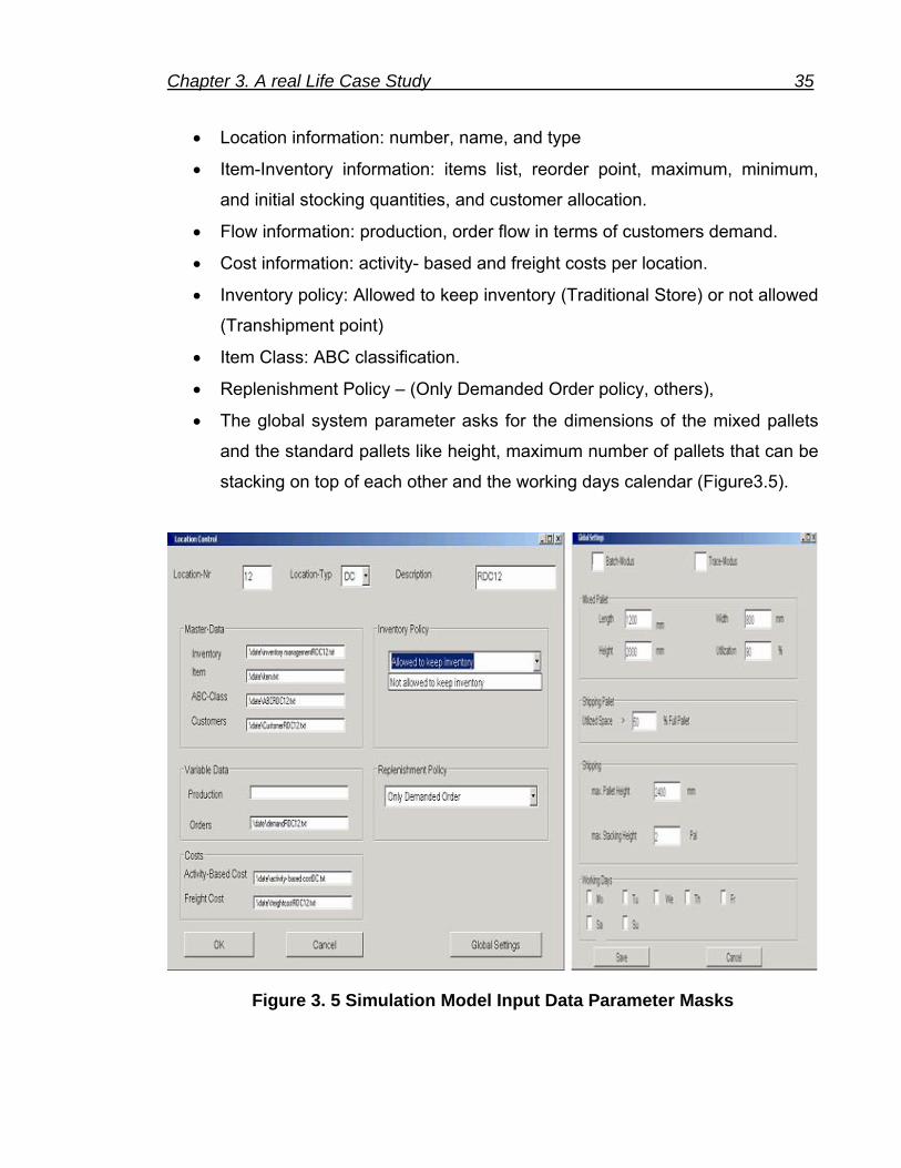
Chapter 3. A real Life Case Study 35
• Location information: number, name, and type
• Item-Inventory information: items list, reorder point, maximum, minimum,
and initial stocking quantities, and customer allocation.
• Flow information: production, order flow in terms of customers demand.
• Cost information: activity- based and freight costs per location.
• Inventory policy: Allowed to keep inventory (Traditional Store) or not allowed
(Transhipment point)
• Item Class: ABC classification.
• Replenishment Policy – (Only Demanded Order policy, others),
• The global system parameter asks for the dimensions of the mixed pallets
and the standard pallets like height, maximum number of pallets that can be
stacking on top of each other and the working days calendar (Figure3.5).
Figure 3. 5 Simulation Model Input Data Parameter Masks

Chapter 3. A real Life Case Study 36
3.2.3. Model Output Reports
The key to the usefulness of a supply chain simulator is the ability to translate the
simulation information into costs and financial reports [BBE98]. This is typically
achieved through the use of activity-based costing models. Therefore, the
developed simulation model generates more detailed information about the activity-
based costs by each location in the network. Once the model has been simulated,
the user can get detailed statistics on almost every aspect of the model's
performance. The data from the simulation has been summarized in a number of
different ways to provide information in the following areas:
• Service Level (Fill rate)
• Transportation
• Inventory
• Activity -based Costs
Some of the standard output reports produced by the model include: financial
summary reports, inventory levels, transportation rate/levels, and service order
degree reports.
3.2.3.1. Financial Summary Report
• Network total cost.
• Detailed network wide expenses, including transportation costs, inventory
carrying costs and activity- based costs.
• Detailed financial split out by site (for all articles): warehousing, inventory,
transportation costs (Table 3.10).

Chapter 3. A real Life Case Study 37
Table 3.10 Activity-Based Cost File of a Distribution Centre
Date and
Time Action
Item -
Nr From To
Sum-
Pal
Pal-
Typ
Sum-
Carton
Pickup-
Carton/Pal Costs
DD.MM.YY
16:00 Ordering - 18 5555 0 0 0 1.2
DD.MM.YY
16:00 Picking A7072 18 5555 1 EP 2 2 0.20
DD.MM.YY
16:00 Picking B8033 18 5555 1 EP 5 5 0.50
DD.MM.YY
16:00 Picking B9134 18 5555 1 EP 5 5 0.50
DD.MM.YY
16:00 Picking A7738 18 5555 1 EP 10 10 1.00
DD.MM.YY
16:00 Picking C7539 18 5555 1 EP 20 20 2.00
DD.MM.YY
16:00 Picking C8855 18 5555 1 EP 5 5 0.50
DD.MM.YY
16:00 Picking D8077 18 5555 1 EP 2 2 0.20 EP: Standard European Pallet
In the above table, the cost per event time for each activity required for one order
per customer is calculated.
3.2.3.2. Inventory Levels
Some reports for tracing inventory are created:
• Detailed tables of inventory status by item, by location, for the entire
network, for the entire run (Table 3.11).
• Aggregated inventory investment, by location, and for the entire network, for
the entire model run (Table 3.12).

Chapter 3. A real Life Case Study 38
Table 3.11 Inventory Tracing File of a Distribution Center
Date and
Time Action Item -Nr Q Stock Min Max
Res-
Q
Back-
Order
In-
Transit
Dlv-
Q.
DD.MM.YY
12:00 RES A9272 120 1549 1549 3874 120 0 0 0
DD.MM.YY
12:00 RES C5833 500 5373 5373 8955 500 0 0 0
DD.MM.YY
12:00 RES C9834 250 5364 5364 13410 250 0 0 0
DD.MM.YY
12:00 RES B7738 188 12356 12356 30890 188 0 0 0
DD.MM.YY
12:00 RES B8939 228 5862 5862 14655 228 0 0 0
DD.MM.YY
12:00 RES D6655 700 3432 3432 5720 700 0 0 0
DD.MM.YY
12:00 RES D6677 260 2583 2583 3874 260 0 0 0 Q: quantity
RES: reservation action.
Res-Q: reserved quantity.
Dlv-Q.: delivered quantity.
In the above table, all inventory actions per event time required for each item are
traceable. The status inventories (stock levels) per event time for each item are
also traceable. This table provides information on the backorder, in-transit, and
delivered quantities for each item.

Chapter 3. A real Life Case Study 39
Table 3.12 Aggregated Ending Inventory File of a Distribution Centre
DC Date and Time
Ending-Inventory
(Pallet)
14 DD.MM.YY 16:00 2586
14 DD.MM.YY 16:00 3224
14 DD.MM.YY 16:00 1258
14 DD.MM.YY 16:00 1169
From the above table, the daily ending inventory and average ending inventory for
one year could be calculated.
3.2.3.3. Transportation Rates/ Levels
For the computation of the transportation costs, a detailed and complex transport
cost matrix has been considered for the calculation based on different calculation
criteria. Some of output files regarding transportation are explained:
• Aggregated toll transportation fees, by location, for the entire network, and
for the entire model run.
• The flow of shipments and the shipment quantity between the locations and
their destinations, for the entire network, and for the entire model run (Table
3.13).
• The transportation frequencies and utilized truck capacity between central
warehouses and distribution centres per location (Table 3.13).
• Tour plan and tour trace by location, for the entire network, and for the entire
model run (Table 3.14 and 3.15).

Chapter 3. A real Life Case Study 40
Table 3.13 Shipment Flow File of one Distribution Centre
DC Date and Time Action Tour Nr From To Nr-Pallet
17 DD.MM.YY 16:00 Shipping T 1 17 4217 6
17 DD.MM.YY 16:00 Shipping T 2 17 3642 9
17 DD.MM.YY 16:00 Shipping T 3 17 3372 20
17 DD.MM.YY 16:00 Shipping T 4 17 3356 15
17 DD.MM.YY 16:00 Shipping T 5 17 2613 30
17 DD.MM.YY 16:00 Shipping T 6 17 1817 4
17 DD.MM.YY 16:00 Shipping T 7 17 1496 8
Table 3.14 Tour Plan File of one Distribution Center
Date and Time
Tour
Nr From To Pal Weight
Freight
Price/Pal Cost
DD.MM.YY 16:00 T 1 17 4217 6 315 20 P 120
DD.MM.YY 16:00 T 2 17 3642 9 722 18 P 162
DD.MM.YY 16:00 T 3 17 3372 20 856 10 P 200
DD.MM.YY 16:00 T 4 17 3356 15 802 12 P 180
DD.MM.YY 16:00 T 5 17 2613 30 978 7 P 210
DD.MM.YY 16:00 T 6 17 1817 4 258 22 P 88
DD.MM.YY 16:00 T 7 17 1496 8 654 18 P 144

Chapter 3. A real Life Case Study 41
Table 3. 15 Tour Trace File of one Distribution Center
Date and
Time Action Item-Nr From To Pal
Pal-
Typ Quantity Weight
DD.MM.YY
16:00 LOAD A6132 17 4217 0,04 EP 20 3.78
DD.MM.YY
16:00 LOAD B8033 17 4217 0,05 EP 30 5.67
DD.MM.YY
16:00 LOAD B6934 17 4217 0,05 EP 30 5.55
DD.MM.YY
16:00 LOAD D8838 17 4217 0,06 EP 30 6.6
DD.MM.YY
16:00 LOAD C7546 17 4217 0,04 EP 20 3.78
DD.MM.YY
16:00 LOAD C9755 17 4217 0,02 EP 10 2.10
DD.MM.YY
16:00 LOAD B4556 17 4217 0,02 EP 10 2.10
DD.MM.YY
16:00 LOAD C5562 17 4217 0,02 EP 10 2.10
DD.MM.YY
16:00 LOAD A6677 17 4217 0,02 EP 12 2.26
3.2.3.4. Service Order Degree Reports
The simulation model generates detailed reports for analysis of the satisfaction of
customer orders by location, for the entire network, and for the entire model run
(Table 3.16).
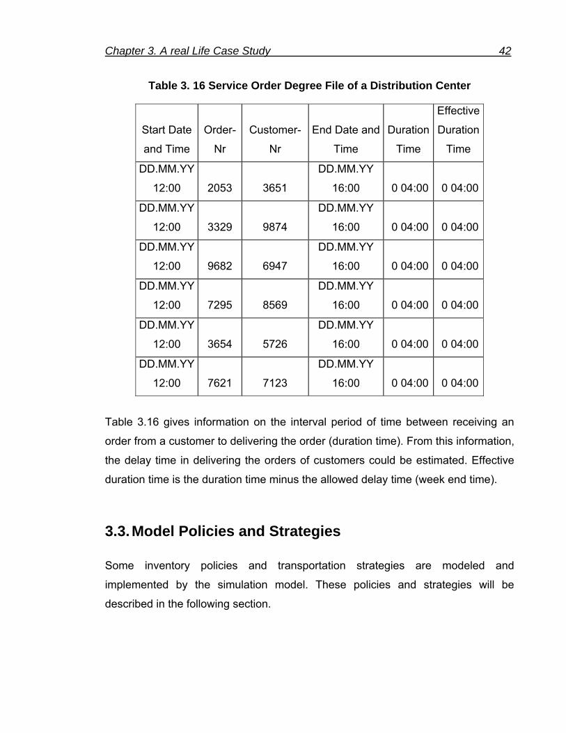
Chapter 3. A real Life Case Study 42
Table 3. 16 Service Order Degree File of a Distribution Center
Start Date
and Time
Order-
Nr
Customer-
Nr
End Date and
Time
Duration
Time
Effective
Duration
Time
DD.MM.YY
12:00 2053 3651
DD.MM.YY
16:00 0 04:00 0 04:00
DD.MM.YY
12:00 3329 9874
DD.MM.YY
16:00 0 04:00 0 04:00
DD.MM.YY
12:00 9682 6947
DD.MM.YY
16:00 0 04:00 0 04:00
DD.MM.YY
12:00 7295 8569
DD.MM.YY
16:00 0 04:00 0 04:00
DD.MM.YY
12:00 3654 5726
DD.MM.YY
16:00 0 04:00 0 04:00
DD.MM.YY
12:00 7621 7123
DD.MM.YY
16:00 0 04:00 0 04:00
Table 3.16 gives information on the interval period of time between receiving an
order from a customer to delivering the order (duration time). From this information,
the delay time in delivering the orders of customers could be estimated. Effective
duration time is the duration time minus the allowed delay time (week end time).
3.3. Model Policies and Strategies
Some inventory policies and transportation strategies are modeled and
implemented by the simulation model. These policies and strategies will be
described in the following section.

Chapter 3. A real Life Case Study 43
3.3.1. Inventory Management Policies
In this simulation model, the location inventory in the supply chain network uses
the continuous review installation stock (s,S) policy where s is the reorder point
and S is the order up-to-level. The stocks are controlled in a decentralized manner
by installation stock reorder points [Axs00]. The simulation model checks
continuously whether the customer orders have reduced the net current inventory
position of any item at each location to a level less than the reorder point (si). When
the net current inventory position falls below the reorder point, the inventory system
will make a replenishment order from the inventory of its upstream location. The
process continues until enough material has been received at the location to fill all
current orders. Net current inventory position is a number calculated throughout the
simulation. The formulas (3.1), (3.2) and (3.3) give expression of the replenishment
(order) quantity.
However, if the stock on-hand cannot fill the order, the order will be held in a queue
in the inventory system; this means the order becomes a backorder. The
backorders are held in a queue in the location. The backorder queue is
implemented as a first-in-first-out (FIFO) queue. Whenever the on-hand, on-order,
and backlog are updated, the net current inventory position (inventory on-hand +
on-order - backorders) will be updated. The inventory system can fill the
backorders only when the replenishment orders (shipments) arrive. There is a time
delay for the shipments to arrive (lead time).
Inventory Tracking files keep track of the possible status of an existing orders that
are open or delivered, and the inventory status include received, in-process, in-
transit, or delivered.
The values of initial inventory on hand, minimum order quantity (si), the maximum
inventory level (Si) and the allowed interval time to stocking for each item type can
be obtained from the Inventory Management files (Table 3.7) as input parameters.

Chapter 3. A real Life Case Study 44
iiii tOtBtHtI )1()1()()( −+−−= (3.1)
∑=
−=N
nniii tRESVtAIVtH
1)()()( (3.2)
If ii stI ≤)(
iii tISQ )(−= (3.3)
Else,
0=iQ
Where
=itI )( inventory position level at time t for item type i .
=itH )( inventory on hand at time t for item type i .
=− itB )1( back-order quantity at time 1−t for item type i .
=− itO )1( on-order quantity at time 1−t for item type i .
=itAIV )( actual inventory level at time t for item type i .
=nitRESV )( reserved customer order quantity of customer order n at time t
for item type i .
=iQ replenishment quantity for item type i .
=is reorder point for item type i .
=iS order-up-to-level for item type i .
=N total number of reserved orders.
Notes:
• The order size is rounds up to make full pallet per item type and the
minimum value of the replenishment quantity is one pallet ( 1=iQ ).
• The customer orders are filled completely or partially (some of available
items).
• The filling of customer orders is based on a first-in-first-out (FIFO) rule.
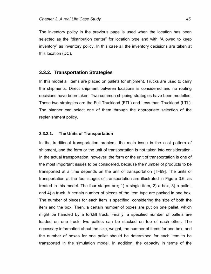
Chapter 3. A real Life Case Study 45
The inventory policy in the previous page is used when the location has been
selected as the “distribution center” for location type and with “Allowed to keep
inventory” as inventory policy. In this case all the inventory decisions are taken at
this location (DC).
3.3.2. Transportation Strategies
In this model all items are placed on pallets for shipment. Trucks are used to carry
the shipments. Direct shipment between locations is considered and no routing
decisions have been taken. Two common shipping strategies have been modelled.
These two strategies are the Full Truckload (FTL) and Less-than-Truckload (LTL).
The planner can select one of them through the appropriate selection of the
replenishment policy.
3.3.2.1. The Units of Transportation
In the traditional transportation problem, the main issue is the cost pattern of
shipment, and the form or the unit of transportation is not taken into consideration.
In the actual transportation, however, the form or the unit of transportation is one of
the most important issues to be considered, because the number of products to be
transported at a time depends on the unit of transportation [TF99]. The units of
transportation at the four stages of transportation are illustrated in Figure 3.6, as
treated in this model. The four stages are; 1) a single item, 2) a box, 3) a pallet,
and 4) a truck. A certain number of pieces of the item type are packed in one box.
The number of pieces for each item is specified, considering the size of both the
item and the box. Then, a certain number of boxes are put on one pallet, which
might be handled by a forklift truck. Finally, a specified number of pallets are
loaded on one truck; two pallets can be stacked on top of each other. The
necessary information about the size, weight, the number of items for one box, and
the number of boxes for one pallet should be determined for each item to be
transported in the simulation model. In addition, the capacity in terms of the

Chapter 3. A real Life Case Study 46
number of pallets to be loaded onto the truck should be decided for each
combination of the supply.
All the above information is given in the item files (Table 3.4) and freight cost per
location files (Table 3.6). Also, information on the pallet dimensions should be
given by the Planner (Figure 3.5).
Figure 3. 6 Units of Transportation
3.4. Model Implementation
This section describes an overview of how the simulation model is implemented.
The modules make use of the DOSIMIS-3 and DLL (C++ Code) interfaces. The
DOSIMIS-3 software interacts with DLL (C++ Code) under the DOSIMIS-3
platform. Each location of the supply chain has text files associated with it. So
whenever the DLL is called, depending on the type of location and the activity to be
executed, the corresponding text file is accessed and data is read or written using
DLL class. Functions and procedures are written in C++ Code to execute the

Chapter 3. A real Life Case Study 47
activities in supply chain, such as, consolidation of items for orders, and delivering
the shipment.
For building supply chain models using DOSIMIS-3 modules, the modules are put
together and connected using their interfaces. So each location in the supply chain
network has its own set of modules (Figure 3.2, 3.3, and 3.4). In addition, text files
corresponding to each location should also be present. These text files and
DOSIMIS-3 modules are linked for each location by DLL under the DOSIMIS-3
platform (Figure 3.5).
DOSIMIS-3 provides a hierarchical modeling. This means that a model can consist
of sub-models. The supply chain simulation model consists of sub-models that
correspond to the modules in the proposed template. The DLL code with the text
files performs planning activities. Execution is carried out under the DOSIMIS-3
environment. Enable processes are modeled as inputs to the simulation either in
the form of text file data or parameters in the DOSIMIS-3 model.
DOSIMIS-3 triggers various scheduling events in DLL either at periodic intervals
(e.g. checking inventory) or based on random events (e.g. customer placing an
order). Some of these types of events are illustrated in Table 3.17.
Table 3. 17 Types of Events Modelled
Event Type Event Description
1 Arrival of a shipment from the Warehouse
2 Place an order from end-customer
3 Update inventory level
4 Starting or Ending Pickup and Consolidation of Orders
5 End of simulation after t years

Chapter 3. A real Life Case Study 48
When DOSIMIS-3 triggers an event, some activities should be achieved by the
DLL Code. For example, when the arrival of an order from the end-customer at the
distribution center occurs then some activities should be executed to fill the order.
The flowchart of order fulfillment control activities at the warehouse and distribution
center locations is shown in Figure 3.7.
End
CheckInventory
Position :< s?(DC)
New CustomerOrder
Arrival (DC)
Reservation Order List (DC)
Determine Reserved Quantity (DC)
Pickup Order List (DC)
Prepare theShipment (DC)
Loading theTruck (DC)
Calculate Transportation Cost (DC)
Tour List (DC)
Dispatch Truck (DC)
Place ReplenishmentOrder to
Warehouse (DC)
ConsolidationList (W)
Pickup Order List (W)
TransportationPlan for
Each DC (W)
Prepare Replenishment Shipment (W)
Loading theTruck (W)
Calculate Transportation
Cost (W)
Tour List (W)
DispatchTruck (W)
Order Arrive/Update
Inventory (DC)
FillBackorders
(DC)
W: Activities done at warehouse locationDC: Activities done at distribution center location
Yes
No
End
CheckInventory
Position :< s?(DC)
New CustomerOrder
Arrival (DC)
Reservation Order List (DC)
Determine Reserved Quantity (DC)
Pickup Order List (DC)
Prepare theShipment (DC)
Loading theTruck (DC)
Calculate Transportation Cost (DC)
Tour List (DC)
Dispatch Truck (DC)
Place ReplenishmentOrder to
Warehouse (DC)
ConsolidationList (W)
Pickup Order List (W)
TransportationPlan for
Each DC (W)
Prepare Replenishment Shipment (W)
Loading theTruck (W)
Calculate Transportation
Cost (W)
Tour List (W)
DispatchTruck (W)
Order Arrive/Update
Inventory (DC)
FillBackorders
(DC)
W: Activities done at warehouse locationDC: Activities done at distribution center location
Yes
No
Figure 3. 7 Flowchart of Order Fulfillment Control Activities at Warehouse and Distribution Center Locations.

Chapter 3. A real Life Case Study 49
Every time a planning activity is carried out, the system status is checked and
actions are taken depending on the status. Information flow can be of two types.
One type of information flow records the status of the system that will be used for
calculating the performance measures. The other type of information flow triggers
events in the model, this includes planning activities that occur while checking the
status of the system and events, such as, placing of an order by the customer. The
simulation progresses due to the triggering of such events.
In addition to the rolled up reports from the model itself, detailed reports are
created for verification and analysis. The simulation model can write detailed data
to text files while the model runs. Collected text files include daily records (such as
inventory for each location for each SKU for each day, order point by location and
SKU, and backorder by Location and SKU). The other text files (output reports)
created for detailed analyses are described the previous sections.
The text files are created for use in an external statistical package such as
Microsoft Excel. Through the results of the simulation analysis, users can assess
the relative merits of alternative supply chains, as well as predict their impact on
costs and delivery.
3.5. Model Optimization
When evaluating a system with many different combinations of possible options, it
can be difficult to execute all possible combinations and identify all of the possible
trade offs. Although users are able to play "what if" with input data and simulation
scenarios to obtain potential solutions, the optimization subsystem helps to
eliminate the need for random trial and error.
In this simulation model, ad hoc approaches that required the user to manually try
many sets of input parameters for optimizing are used [SP00].

Chapter 3. A real Life Case Study 50
3.6. A Real-Life Case Study
3.6.1. A Real Distribution Supply Chain Description
A real life distribution supply chain in a food industry has been considered. The
company is located in a European country, produces three major brands of
products, and holds more than 3000 different SKUs per day (stock keeping unit).
Currently, this company has several production locations (plants), central
warehouses, about 30 regional distribution centres, and approximately more than
5000 retailers and customers spread over the country. The warehouses are
located at the plants and deliver different items to distribution centres which in turn
supply a large set of geographically scattered retailers. It is assumed that the
warehouses replenish multi-items from infinite supply plants and act merely as
coordinators of the supply process, but do not hold any stocks.
The distribution centres hold stocks of multi-items and use common inventory
policies to replenish their inventory levels. Each distribution centre faces a dynamic
demand rate. Figures 3.8 shows the distribution supply chain network considered
with the dynamic of flow orders; and Figure 3.9 shows the locations inside the
country.

Chapter 3. A real Life Case Study 51
Figure 3. 8 A Real Distribution Supply Chain Network
Figure 3. 9 Plants and Distribution Centers Location

Chapter 3. A real Life Case Study 52
The detailed description of the model considered has been presented in the
following section:
3.6.2. Model Data and Analysis
A significant amount of historic data from the company’s ERP (Enterprise
Resource Planning) system has been used to conduct the simulation study. In the
first phase of the simulation study, an extensive data analysis was accomplished.
In this study only 3 plants, 3 warehouses, and 24 regional distribution centres
(RDCs) are included. The distribution centres have different size of customers
(small, medium, and large). Five distribution centres with small-sized customers
are assumed to operate as local distribution centres (LDCs) and are not
responsible for delivering to their customers. The customers receive their orders
by an own truck fleet. The 19 regional distribution centres that have medium and
large-sized customers are responsible for delivering to their customers.
3.6.2.1. Items (Articles) Data
Different types of items are produced by the plants. In total, the items are produced
in 392 different types. The plants’ production is enough to meet orders received
daily. Figure 3.10 shows the number of different item types for each plant.

Chapter 3. A real Life Case Study 53
94
82
216
0
50
100
150
200
250
Plant1 Plant2 Plant3
Plant Number
Num
ber o
f Ite
ms
Figure 3. 10 Number of Item Types per Plant
The items have different characteristics (name, weight, and volume). The
distribution centres keep stocks of multi-item (SKU) and use the three warehouses
to replenish their inventory levels. Each distribution centre holds different types of
items. The number and percentage of different item types replenished from each
warehouse to each distribution centre is shown in Figure 3.11.

Chapter 3. A real Life Case Study 54
37 36 38 34 39 46 41 36 36 38 38 35 38 37 38 36 42 36 38 29 30 26 27 31
13 13 13 1314
14 1213 12 13 13 13 13 14 13 13 13 13 13 12
1212 12 13
56 59 62 57 57 74 61 60 60 59 58 59 62 64 61 55 70 58 58 47 44 44 42 48
0%
20%
40%
60%
80%
100%
RDC1RDC2
RDC3RDC4
RDC5RDC6
RDC7RDC8
RDC9
RDC10
RDC11
RDC12
RDC13
RDC14
RDC15
RDC16
RDC17
RDC18
RDC19LD
C1LD
C2LD
C3LD
C4LD
C5
Distribution Center
Num
ber
of It
ems
(%)
Warehouse(1) Warehouse(2) Warehouse(3) Figure 3. 11 Number and Percentage of Replenished Items from each
Warehouse type to each Distribution Center
3.6.2.2. Customer Orders Data and Analysis
The following set of customer information has been considered in the simulation
model:
• Customer name
• Customer number
• Address
• Travel Distance from the regional distribution centres
• Type of customer
The customer orders for each distribution centre for one year are also collected
from the company and have been analyzed. Each distribution center receives daily
orders of different items (order lines) from retailers and customers. Figure 3.12

Chapter 3. A real Life Case Study 55
illustrates the average daily number of order lines per distribution center. The total
number of customers and retailers at each distribution center is presented in Figure
3.13.
22 2326 25 24 24 24 24
2623
2124
29
2522 21
26 2523
47 4643
51 52
0
10
20
30
40
50
60
RDC1RDC2
RDC3RDC4
RDC5RDC6
RDC7RDC8
RDC9
RDC10
RDC11
RDC12
RDC13
RDC14
RDC15
RDC16
RDC17
RDC18
RDC19LD
C1LD
C2LD
C3LD
C4LD
C5
Distribution Center
Avg
. Ord
er L
ines
Figure 3. 12 Average Number of Order Lines per Distribution Center

Chapter 3. A real Life Case Study 56
Figure 3. 13 Number of Customers per Distribution Center
The average daily demand for each item is aggregated and fitted to some of the
theoretical probability distributions by using Input Analyzer. The Input Analyzer is a
standard tool that accompanies ARENA software and is designed specifically to fit
distributions to observed data, provide estimates of their parameters, and measure
how well they fit into the data. In addition, the Input Analyzer provides three
numerical measures of the quality of fit of a distribution to the data. The first, and
the simplest to understand, is the mean square error. This is the average of the
square error terms for each histogram cell, which are the squares of the
differences between the relative frequencies of the observations in a cell and the
relative frequency for the fitted probability distribution function over that cell’s data
range. The larger this square error value, the further away the fitted distribution is
from the actual data (and thus the poorer the fit). The other two measures of a
distribution’s fit to the data are the chi-square and Kolmogorov-Smirnov (K-S)
goodness-of-fit hypothesis tests. Kelton et al. [KSS02] gives more information
about these tests and the Input Analyzer.
195210
175117
178592
230332
195230
319200
189196
542362
248298
28500000
0 100 200 300 400 500 600 700
RDC1RDC2RDC3RDC4RDC5RDC6RDC7RDC8RDC9
RDC10RDC11RDC12RDC13RDC14RDC15RDC16RDC17RDC18RDC19
LDC1LDC2LDC3LDC4LDC5
Dis
trib
utio
n C
ente
r
Number Of Customers

Chapter 3. A real Life Case Study 57
Figure 3.14 shows the aggregated daily average demand, the standard deviation,
and the coefficient of variation (CV). Table 3.18 presents the fitted probability
distribution with the square error for each distribution centre.
0
50
100
150
200
250
300
RDC1RDC2
RDC3RDC4
RDC5RDC6
RDC7RDC8
RDC9
RDC10
RDC11
RDC12
RDC13
RDC14
RDC15
RDC16
RDC17
RDC18
RDC19LD
C1LD
C2LD
C3LD
C4LD
C5
Distribution Center
Qua
ntity
(Pal
let)
0
0,1
0,2
0,3
0,4
0,5
0,6
CV
Average Daily Aggregate Demand (Pallet) Standard Deviation CV
Figure 3. 14 Aggregated Average Daily Demand

Chapter 3. A real Life Case Study 58
Table 3. 18 Fitted Probability Distribution per Distribution Center
The percentage of each probability distribution of demand are calculated from the
above Table and shown in Figure 3.15
DC Probability Distribution Square ErrorRDC1 Gamma 0.005490RDC2 Erlang 0.005352RDC3 Weibull 0.005104RDC4 Lognormal 0.004430RDC5 Gamma 0.010967RDC6 Normal 0.009840RDC7 Normal 0.008318RDC8 Normal 0.004959RDC9 Normal 0.003856
RDC10 Normal 0.009327RDC11 Gamma 0.006381RDC12 Gamma 0.007801RDC13 Beta 0.010409RDC14 Normal 0.007741RDC15 Normal 0.005139RDC16 Normal 0.006693RDC17 Normal 0.005081RDC18 Normal 0.008071RDC19 Normal 0.003365LDC1 Lognormal 0.007407LDC2 Poisson 0.005243LDC3 Lognormal 0.005141LDC4 Beta 0.006377LDC5 Erlang 0.005882

Chapter 3. A real Life Case Study 59
8%8%
17%
46%
13%
4% 4%
Beta Erlang Gamma Normal Lognormal Poisson Weibull
Figure 3. 15 Percentage of each Probability Distribution of Demand
When dealing with real supply chain problems, one of the important aspects is to
consider whether the different items are homogeneous in terms of demand
(demand variability). Demand variability ranges widely in different industries. For
example, daily demand variability may be low (CV = 0.1 to 0.3) in consumer
products but significantly higher in electronics products due to short product life
cycles [WJD99]. To see the complexity and sensitivity of the considered real
model, an analysis of demand data for individual items has been performed to
evaluate the differences between items. The demand generated at the DC as real
demand is considered.
A daily total average demand and standard deviation of 2546 items has been
calculated, and then the CV is calculated and is shown in Figure 3.16.

Chapter 3. A real Life Case Study 60
0,93
0,84
0,94
0,81
0,98
0,83
0,96 0,960,99
1,1
0,84
0,69
0,760,79
0,74
0,910,91
0,93
0,920,93
0,960,9
0,960,95
0
0,2
0,4
0,6
0,8
1
1,2
RDC1RDC2
RDC3RDC4
RDC5RDC6
RDC7RDC8
RDC9
RDC10
RDC11
RDC12
RDC13
RDC14
RDC15
RDC16
RDC17
RDC18
RDC19LD
C1LD
C2LD
C3LD
C4LD
C5
Distribution Center
CV
Average of CV per Item Avg.
Figure 3. 16 Average of the Coefficient of Variation per Item for each Distribution Center
As can be seen from Figure 3.16, the CV of each item is higher than 0.5. This
means that the demand variability is significantly high. Therefore, the considered
real model is very sensitive and complex.
3.6.2.3. Lead Times
The lead times between locations (Warehouses and Distribution centres) are
assumed to be uniformly distributed from 1 to 4 working days.
3.6.2.4. Logistics Cost Structure
In this study the most common (practice) and complex logistics cost structures
have been considered. The logistics costs can be classified as follows:

Chapter 3. A real Life Case Study 61
• Transportation costs: The transportation cost is the most complex cost
structure. A detailed transport cost matrix from the company has been
considered for the computation of the transport costs based on different
calculation criteria. The criteria depend on the number of pallets, weight,
and distance (ZIP code and region). Freight rate discounts are offered
based on these criteria and considered in the simulation model. The
distance matrix between all the warehouses and distribution centres is
shown in Table 3.19. The reduction of transportation cost (%) offered by
Third Party Logistics (3PL) provider from warehouse 2 to three distribution
centre (RDC9, RDC13 and RDC19) is explained in Table 3.20.
• Storage and handling costs (inventory costs)
a) Monthly storage costs
b) Order costs
• Activity-Based Costs
c) Order picking costs per pallet
d) Warehouse outgoing goods costs per pallet
e) Regional distribution centres incoming goods costs per pallet
• Toll fees
f) Inbound toll costs (warehouse to distribution centres) per kilometre
travelled.
g) Outbound toll costs (distribution centres to retailers and customers)
per kilometre travelled.

Chapter 3. A real Life Case Study 62
Table 3. 19 Distance Matrix in Kilometers
D C W a r e h o u s e ( 1 ) W a r e h o u s e ( 2 ) W a r e h o u s e ( 3 )R D C 1 5 1 9 6 5 3 2 8 5R D C 2 4 4 3 6 4 7 2 1 4R D C 3 4 4 8 5 4 9 2 6 7R D C 4 3 8 6 4 3 0 2 0 4R D C 5 2 8 3 5 2 1 1 2 7R D C 6 0 2 7 0 2 5 7R D C 7 3 2 2 1 9 2 3 8 8R D C 8 3 9 7 5 9 6 1 6 3R D C 9 3 0 0 5 8 4 7 3
R D C 1 0 2 5 0 2 5 8 2 3 6R D C 1 1 5 2 5 4 6 7 4 0 4R D C 1 2 5 8 0 4 5 1 5 8 9R D C 1 3 5 9 6 6 9 7 3 9 8R D C 1 4 1 3 7 3 5 8 1 5 2R D C 1 5 9 2 1 8 3 2 9 6R D C 1 6 2 2 6 1 3 6 3 8 3R D C 1 7 2 3 9 4 0 1 5 7R D C 1 8 2 5 7 4 4 3 0R D C 1 9 4 3 8 1 9 5 5 5 2L D C 1 5 9 0 6 9 1 3 9 9L D C 2 5 1 3 2 7 0 6 3 6L D C 3 1 9 5 1 0 4 3 6 2L D C 4 6 8 5 5 5 5 5 6 1L D C 5 4 8 8 5 3 9 3 0 6
Table 3. 20 Reduction in Transportation Cost (%) Matrix
R D C 9 R D C 1 3 R D C 1 92 1 1 0 , 0 0 % 0 , 0 0 % 0 , 0 0 %2 2 2 3 3 , 9 1 % 5 , 6 8 % 3 4 , 7 8 %2 3 3 4 1 , 9 6 % 1 1 , 3 6 % 4 1 , 3 0 %2 4 4 5 1 , 9 6 % 2 1 , 5 9 % 4 3 , 4 8 %2 5 5 5 9 , 1 3 % 3 7 , 5 0 % 4 6 , 7 4 %2 6 6 6 3 , 9 1 % 4 0 , 1 1 % 4 7 , 3 9 %2 7 7 6 7 , 3 9 % 4 2 , 0 5 % 5 0 , 2 2 %2 8 8 7 0 , 0 0 % 4 4 , 2 0 % 5 3 , 4 8 %2 9 9 7 2 , 6 1 % 4 5 , 6 8 % 5 6 , 0 9 %2 1 0 1 0 7 4 , 7 8 % 4 6 , 1 4 % 5 8 , 0 4 %2 1 1 1 1 7 6 , 9 6 % 4 7 , 1 6 % 6 0 , 6 5 %2 1 2 1 2 7 8 , 2 6 % 4 8 , 6 4 % 6 2 , 3 9 %2 1 3 1 3 7 9 , 1 3 % 5 0 , 6 8 % 6 3 , 7 0 %2 1 4 1 4 7 9 , 7 8 % 5 1 , 1 4 % 6 5 , 0 0 %2 1 5 1 5 8 0 , 2 2 % 5 4 , 0 7 % 6 6 , 0 9 %2 1 6 1 6 8 0 , 8 7 % 5 4 , 8 9 % 6 7 , 6 1 %2 1 7 1 7 8 1 , 3 0 % 5 6 , 1 4 % 6 8 , 9 1 %2 1 8 1 8 8 1 , 5 2 % 5 6 , 5 9 % 7 0 , 2 2 %2 1 9 1 9 8 1 , 9 6 % 5 6 , 5 9 % 7 1 , 3 0 %2 2 0 2 0 8 2 , 1 7 % 5 6 , 8 2 % 7 2 , 1 7 %2 2 1 2 1 8 2 , 8 3 % 5 7 , 0 5 % 7 3 , 4 8 %2 2 2 2 2 8 3 , 4 8 % 5 7 , 1 6 % 7 4 , 3 5 %2 2 3 2 3 8 4 , 1 3 % 5 7 , 2 7 % 7 5 , 2 2 %2 2 4 2 4 8 4 , 7 8 % 5 7 , 3 9 % 7 6 , 0 9 %2 2 5 2 5 8 5 , 0 0 % 5 7 , 3 9 % 7 6 , 7 4 %2 2 6 2 6 8 5 , 0 0 % 5 7 , 5 0 % 7 6 , 9 6 %2 2 7 2 7 8 5 , 2 2 % 5 7 , 5 0 % 7 7 , 1 7 %2 2 8 2 8 8 5 , 4 3 % 5 7 , 5 0 % 7 7 , 3 9 %2 2 9 2 9 8 5 , 6 5 % 5 7 , 6 1 % 7 7 , 6 1 %2 3 0 3 0 8 5 , 8 7 % 5 7 , 6 1 % 7 7 , 8 3 %2 3 1 3 1 8 6 , 0 9 % 5 7 , 7 3 % 7 8 , 0 4 %2 3 2 3 2 8 6 , 3 0 % 5 7 , 8 4 % 7 8 , 4 8 %2 3 3 3 3 8 6 , 5 2 % 5 7 , 9 5 % 7 8 , 7 0 %2 3 4 3 4 8 6 , 7 4 % 5 8 , 6 4 % 7 8 , 9 1 %2 3 5 3 5 8 6 , 9 6 % 5 9 , 0 9 % 7 9 , 1 3 %2 3 6 3 6 8 6 , 9 6 % 5 9 , 5 5 % 7 9 , 3 5 %2 3 7 3 7 8 7 , 1 7 % 5 9 , 7 7 % 7 9 , 7 8 %2 3 8 3 8 8 7 , 3 9 % 6 0 , 2 3 % 8 0 , 4 3 %
D i s t r i b u t i o n C e n t e r N r .W a r e h o u s e N r . P a l m i n P a l m a x

Chapter 3. A real Life Case Study 63
As can be seen from Table 3.20, as the number of shipped pallets is increased the
transportation cost is reduced. The percentage of this reduction varies for each
warehouse and for each distribution center. More analysis will be discussed in
Chapter 5.
3.6.3. Problem Description
Due to increasing logistics costs and due to considerable competition in the market
the company wants to build and use a simulation model to study and investigate
many different optimizing decisions regarding distribution network structures and
distribution strategies. The company is also interested in studying the proper
measures of performance that should be used. A primary objective was to maintain
or improve service levels, while reducing inventories and transportation costs. A
project team used simulation to quantify how well alternative networks would
function through variations in demand and supply. The company designed some
different scenarios and requires the following questions to be answered by the
simulation model:
1. Is the existing distribution network well designed?
2. What is the optimal distribution network from the proposed scenarios?
3. How should new cost structures be considered and evaluated?
4. What is the relationship between distribution strategies and the resulting
inventory levels, customer service levels, and number of replenishments?
5. Does the location of inventory storage for different classes of item have an
effect on the total inventory levels and number of tours?
The logistics manager in the company had to study some operating strategies to
evaluate and improve the existing network. The simulation study was designed to
investigate these strategies.

Chapter 3. A real Life Case Study 64
3.6.4. Simulation Model and Assumptions
The main objective of applying the simulation was the investigation of different
operating strategies at the warehouses and regional distribution centres to improve
the efficiency of the distribution network in the supply chain. The simulation model
which has been developed and described at the beginning of this chapter is
implemented. Figure 3.17 illustrates a snapshot screen of the simulation model.
Figure 3. 17 DOSIMIS-3 Simulation Model Snapshot
3.6.4.1. Simulation Assumptions
The developed simulation model was implemented under the following
assumptions:

Chapter 3. A real Life Case Study 65
• Standard European Pallet (SEP) with a height of 2.4 m height will be used to
move the full pallet product from the warehouses to regional distribution
centre.
Length x Width x Height (LxWxH) = 1.2m x 0.8m x 2.4m
• The mixed pallet of the following dimensions will be used to move the
product from the regional distribution centre to retailers and customers :
L x W x H = 1.2m x 0.8m x 1.8m. Percentage of utilized space: 70%
• Transportation costs based on the direct tour with one destination will be
accounted, no routing allowed.
• Direct shipments from central warehouse to retailers or customers are
allowed if the shipment size is up to truck capacity.
• The used truck capacity is 38 SEP
• All transportations between locations are done by Third Party Logistics
(3PL) providers. Therefore the fixed transportation costs are not considered.
• The customer orders are satisfied and delivered completely (all order lines)
based on a first-in-first-out (FIFO) rule.
3.6.5. Simulation Experiment and Results
Simulation results are collected after running the developed simulation model for
one year. The validation of the model has been accomplished by comparing the
simulated results with the historical data provided by the logistic department in the
company. The data collected for each scenario is exported to an Excel worksheet
after the simulation run is completed. Noche et al. [NAH04] gives more detailed
information about these scenarios, the answer to the previously raised questions,
and the findings.

Chapter 3. A real Life Case Study 66
3.7. Extended Studies and Models
Coordination and Integration are the key terms for effective supply chain
management. An effective supply chain will reduce the systemwide costs while
improving the service levels and conforming to customer requirements.
In last few years, as many companies become aware of their supply chain
performance and the importance of their performance improvement, coordination
and integration of the inventory and the distribution strategies have become the
other source of competitive advantages. They have also realized that important
cost savings can be achieved by integrating inventory control and transportation
policies throughout their supply chains. Thus, the problem faced by these
companies is to find an optimal replenishment plan, i.e. an inventory and
transportation strategy, so as to minimize total inventory and transportation costs
over a finite planning horizon [CMS02].
The problem has attracted the attention of researcher in recent years and many
models have been proposed in this direction. The basic idea behind these models
is to simultaneously optimize decision variables of different stages that have
traditionally been optimized sequentially, in the sense that the optimized output of
one stage becomes the input to the other stage (first setting inventory levels and
then scheduling distribution, for instance). Since the problem is so complex that
optimal solutions are very difficult to obtain. Due to this reason most of the study
models consider simple networks and make many assumptions, such as, only
considering direct shipment, in order to simplify the problem, and thus, it can be
solved by exact algorithms (mixed integer programming) and heuristic solution
approaches.
Integrated inventory replenishment and order shipment consolidation have
received much attention recently, driven mainly by the widespread adoption of
Vendor Managed Inventory (VMI) programs. Under a typical VMI program, the
supplier/vendor holds a certain level of control not only over in-bound

Chapter 3. A real Life Case Study 67
replenishment decisions on stocking, but also over outbound re-supply decisions
on the timing and/or quantity of shipment consolidation. Thus, the trucks are more
likely to be dispatched fully, and the vendor has a better opportunity to synchronize
the inventory and transportation decisions. However, the challenge is to satisfy
demanding customer service standards if they are justified, while at the same time
the benefits of consolidation are achieved.
Generally, to solve such integrated problems optimally and to implement such
concepts is not easy due to their combinatorial and dynamic nature, especially
when many strategies are involved in a real supply chain.
Simulation models that permit user interaction and take the dynamics of the system
in to account are capable of characterizing system performance for integrated
models.
The previous open problems and new concepts regarding these problems are
mainly the scope of work of this thesis. Many extended studies and experiments
have been constructed and conducted. In the next sections, detailed description of
the extended studies of the case study and the developed simulation model will be
introduced.
3.7.1. Investigation of Coordinating Distribution Strategies and Inventory Policies Study
The goal of this work is the study of the integrated inventory and distribution
problem which is concerned with coordinating the inventory and delivery operations
to meet customer demand with an objective to minimize the total logistic costs. The
developed simulation model is used to investigate the effect of coordination and
integration of inventory policies and distribution strategies on the selected
measures of performance and also to see how significantly the coordination affects
the selected measures of performance.

Chapter 3. A real Life Case Study 68
In this study, the existing distribution supply chain network is extended to be more
complex. The considered network consists of three echelons (Warehouse,
distribution centre, and special retailer). Many simulation scenarios have been
designed and many statistical tests have been performed to see how significantly
the coordination affects the selected measures of performance.
The results from statistical test approach suggest that the inventory policies and
shipping (distribution) strategies significantly affect the measures of performance of
the supply chain network. The investigations also show that integrating the
inventory policies and transportation strategies is not simple. It requires a trade-off
between different performance measures. Potential costs saving can be achieved
by selecting the right inventory policy and transportation strategy. The complete
benefit of coordination is only achieved when all the stages and functions in the
entire network are integrated. Housein et al. [HAN05] gives more detailed
description of this work. The results of this study clearly conform to intuition and
help to verify the internal consistency of the developed simulation model. There are
many opportunities for expansion of the simulation model presented in this study.
The open areas where model expansion would be of benefit are discussed and
carried out in the subsequent sections of this thesis.
3.7.2. Coordination Strategies Model Study II
One of the current interests in supply-chain management is to overlook certain
transportation/distribution issues; potential savings are realizable by carefully
coordinating a shipment strategy with the inventory replenishment policies. This
effect is particularly tangible when the shipment strategy calls for a consolidation
program where several smaller deliveries are shipped as a single load, realizing
substantial savings in transportation costs.
Formally, shipment consolidation refers to the active intervention by management
to combine many small shipments/orders so that a larger, hence more economical,

Chapter 3. A real Life Case Study 69
load can be sent on the same vehicle [Bre81], [Hal87], [HB95]. The main
motivation behind a consolidation program is to take advantage of the decreased
per unit freight costs due to economies of scale associated with transportation
[CL00]. Based on that two heuristic, consolidation concepts are developed and
programmed to integrate into the developed simulation model. These two are:
1. Item classification consolidation concept
2. N-days forecasted demand concept
The flow logical processes for both consolidation concepts are illustrated in Figure
3.18.
Select Appropriate Group (items)
For Consolidation
Receive an OrderOf Multi-Items
(at Distribution Center)
Some Items Reach its Reorder Point and Trigger
A Group Replenishment
Select ConsolidationConcept
Estimate AppropriateGroup Consolidation
Quantity
Place Consolidated Replenishment Order
(at Distribution Center)
Is Quantities of A Group Replenishment
< Truck Capacity?
Yes
No
Examine InventoryPosition of each Item
Send (Normal or Consolidated)Replenishment Shipment
(at Warehouse)
Place an NormalReplenishment Order
(at Distribution Center)
Figure 3.18 Flow Logical Processes of Consolidation Concept

Chapter 3. A real Life Case Study 70
3.7.2.1. Notation
jQR = replenished quantity for item j in pallet unit.
iQC = consolidated quantity for item i in pallet unit.
iDQ = customer order quantity for item i (in pallet unit) of one day.
iNQ = sum of order quantities for item i (in pallet unit) of the next N-days.
CTr = truck capacity.
ECTr = empty truck capacity.
iI = inventory position for item i .
is = reorder point
RL= replenishment list.
CL= consolidation list.
NDL= N-days list.
CNDL= candidate items N-days list.
FCL= final consolidation list.
FCNDL= final consolidation of candidate items list.
n = number of items.
N = total number of days.
The two consolidation concepts are constructed under the following two
assumptions:
• The replenished quantity ( jQR ) and consolidated quantity ( iQC ) rounded up
to make full pallet per item type, and the minimum quantity is one pallet.
• The total quantities of group replenishment are less than the truck load
(truck capacity).
For more understanding of the consolidation concepts, some steps are
summarized. In the following section, the steps of the consolidation concepts are
presented.
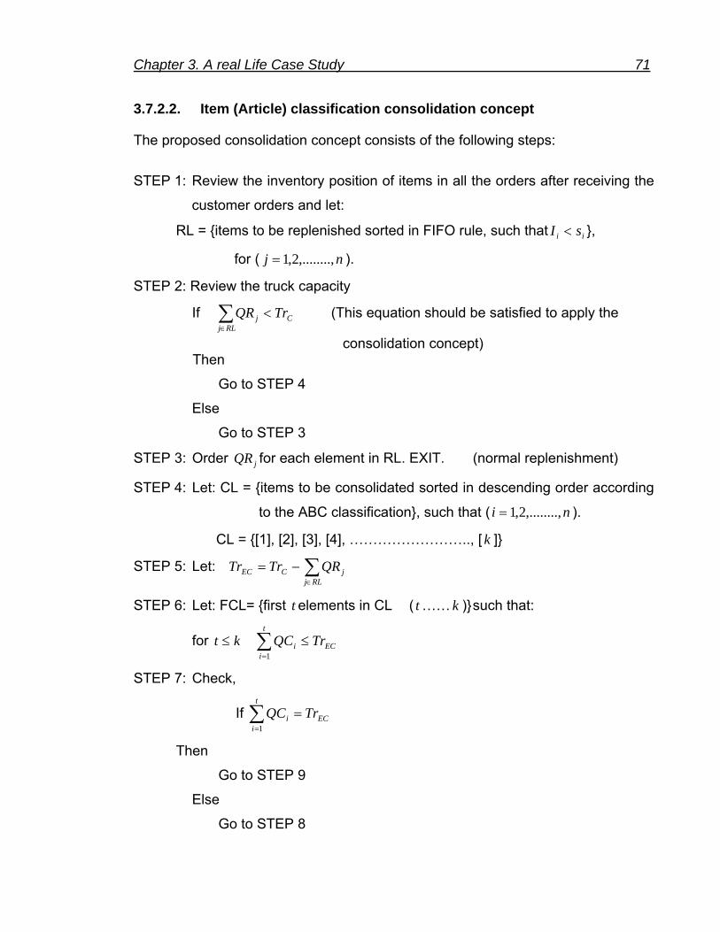
Chapter 3. A real Life Case Study 71
3.7.2.2. Item (Article) classification consolidation concept
The proposed consolidation concept consists of the following steps:
STEP 1: Review the inventory position of items in all the orders after receiving the
customer orders and let:
RL = {items to be replenished sorted in FIFO rule, such that ii sI < },
for ( nj ,........,2,1= ).
STEP 2: Review the truck capacity
If CRLj
j TrQR <∑∈
(This equation should be satisfied to apply the
consolidation concept) Then
Go to STEP 4
Else
Go to STEP 3
STEP 3: Order jQR for each element in RL. EXIT. (normal replenishment)
STEP 4: Let: CL = {items to be consolidated sorted in descending order according
to the ABC classification}, such that ( ni ,........,2,1= ).
CL = {[1], [2], [3], [4], …………………….., [ k ]}
STEP 5: Let: ∑∈
−=RLj
jCEC QRTrTr
STEP 6: Let: FCL= {first t elements in CL ( t …… k )} such that:
for kt ≤ EC
t
ii TrQC ≤∑
=1
STEP 7: Check,
If EC
t
ii TrQC =∑
=1
Then
Go to STEP 9
Else
Go to STEP 8
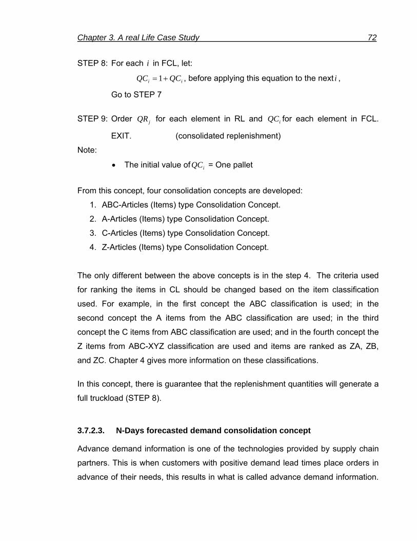
Chapter 3. A real Life Case Study 72
STEP 8: For each i in FCL, let:
ii QCQC += 1 , before applying this equation to the next i ,
Go to STEP 7
STEP 9: Order jQR for each element in RL and iQC for each element in FCL.
EXIT. (consolidated replenishment)
Note:
• The initial value of iQC = One pallet
From this concept, four consolidation concepts are developed:
1. ABC-Articles (Items) type Consolidation Concept.
2. A-Articles (Items) type Consolidation Concept.
3. C-Articles (Items) type Consolidation Concept.
4. Z-Articles (Items) type Consolidation Concept.
The only different between the above concepts is in the step 4. The criteria used
for ranking the items in CL should be changed based on the item classification
used. For example, in the first concept the ABC classification is used; in the
second concept the A items from the ABC classification are used; in the third
concept the C items from ABC classification are used; and in the fourth concept the
Z items from ABC-XYZ classification are used and items are ranked as ZA, ZB,
and ZC. Chapter 4 gives more information on these classifications.
In this concept, there is guarantee that the replenishment quantities will generate a
full truckload (STEP 8).
3.7.2.3. N-Days forecasted demand consolidation concept
Advance demand information is one of the technologies provided by supply chain
partners. This is when customers with positive demand lead times place orders in
advance of their needs, this results in what is called advance demand information.

Chapter 3. A real Life Case Study 73
Ford Motor Company, for example, issues and weekly updates orders to its
catalytic converter suppliers, as discussed in the “Corning Glass Works” Harvard
Business School teaching case (1991). The e-commerce of customized products,
such as personal computers, provides advance demand information for the product
components. An example is Dell’s cutting edge distribution model. Under this
model, consumers are allowed to customize their choice of PC online for future
delivery [HS99].
Toyota recently announced plans to make customized cars within five days,
reflecting its ability to quickly respond to advance demand information [Sim99]. GM
and Ford are scrambling to catch up this trend. These strategies, in conjunction
with advances in information technology, assist companies in getting a better
sense of demand and its evolution over time.
Advance demand information enables many companies to shift their production
operations from the ‘build to stock’ to ‘build to order’ model. In spite of the fact that
many companies operate in a dynamic environment, stochastic inventory models
that incorporate advance demand information are rare [GÖ01].
In addition, advance information technology allows supply chains to be designed to
satisfy most of the conflicting goals. For example, when shipments are delivered in
full truckloads, this is done to minimized transportation costs, and at the same time,
it leads to higher inventory costs. Such conflicting cases can be reduced by using
advance information technology [SKS03]. In this thesis, this fact has been
implemented by applying the developed consolidation concept (N-Days forecasted
demand consolidation).
The proposed concept for the consolidation is modified to consider the above
technology and consists of the following steps:

Chapter 3. A real Life Case Study 74
STEP 1: Review the inventory position of items in all the orders after receiving the
customer orders and let: RL = {items to be replenished, sorted in FIFO
rule, such that ii sI < }, for ( nj ,........,2,1= ).
STEP 2: Review the truck capacity
If C
RLjj TrQR <∑
∈
(This equation should be satisfied to apply the
consolidation concept) Then
Go to STEP 4
Else
Go to STEP 3
STEP 3: Order jQR for each element in RL. EXIT. (normal replenishment)
STEP 4: Read all orders for the next N-days for each DC from the order customers
list.
Let: NDL = {items to be ordered in N-days ranked by event time,
following chronological order}, for ( ni ,........,2,1= ).
STEP 5: Sum all the order quantities for the same item at the same location.
Let: ∑=
=N
DiDiN QQ
1 for each i in NDL
STEP 6: Check, for each i in NDL
If iiN IQ >
Then
Go to STEP 7
Else
Go to STEP 6
STEP 7: Let: CNDL= {candidate items for consolidation, such that iiN IQ > }, for
( ni ,........,2,1= )
If CNDL= {ø} then Go to STEP 3
STEP 8: Rank the k items in CNDL following the same sequence in NDL, such
that: CNDL= {[1], [2], [3], [4],………….[ k ]}

Chapter 3. A real Life Case Study 75
STEP 9: For each i in CNDL set:
iNi QQC =
STEP 10: Let:
∑∈
−=RLj
jCEC QRTrTr
STEP 11: Let: FCNDL= [first t elements in CNDL ( t ….. k )} such that
for kt <
EC
t
ii TrQC ≤∑
=1 and EC
t
iim TrQCQC >+∑
=
)(1
for each tm > and m in CNDL
Go to STEP 12
for kt = :
EC
t
ii TrQC ≤∑
=1
Go to STEP 13
STEP 12: Let ∑=
−=t
iiECm QCTrQC
1 ( m is the last item in FCNDL)
STEP 13: Order jQR for each element in RL and iQC for each element in FCNCL.
EXIT. (consolidated replenishment)
As mentioned before, this concept is constructed under an important assumption.
The assumption is:
• Advance information about the order of customers is incorporated.
This assumption is valid because many companies in the industry ask customers
to fix their demands some days before the delivery. Therefore, in this thesis, the
concept using this technology is implemented.
Due to fact that information technology has developed in recent years and
companies are seldom willing to incorporate such technology into the original

Chapter 3. A real Life Case Study 76
consolidation concept, this technology is not considered. The original concept is
constructed under another assumption:
• Forecasting techniques are used to forecast a demand in advance.
Therefore, Step 4 should be modified, and instead the order customers list should
be read for n-days, by applying any forecasting technique, reading from the
forecasted demand list for n-days.
Also, a discussion is held with the logistics manager in the considered company
regarding the maximum period for which information is required from the
customers in advance. The maximum period is not more than four days. Based on
that two consolidation concepts are developed:
1. 2-Days Forecasted Demand Consolidation Concept.
2. 4-Days Forecasted Demand Consolidation Concept.
In this concept, there is no guarantee that the replenishment quantities will
generate a full truckload. More detailed information about the classification of items
and the application of the consolidation concepts is described in the next chapter.
3.7.3. VMI-Programs Model Study II
In this study, a simulation model for coordinating inventory and transportation
decisions in VMI systems is presented. The mechanism driving order placement is
the only modification made for the developed simulation model. Instead of the
distribution centre placing orders with the warehouse (supplier), the warehouse
obtains customer orders directly, bypassing the distribution centre. In turn, the
warehouse determines the quantity and timing of goods sent to the distribution
centre, and the distribution centre functions primarily not only as a transport delay
in the system, (transshipment point) but also as a rearrangement for the tours.

Chapter 3. A real Life Case Study 77
Note that the distribution centre no longer places orders with the warehouse.
Distribution centre inventory is depleted at a rate, by retail shipping, which is equal
to customer demand.
To reflect the vendor-managed inventory concept by using the developed
simulation model, the user should select the appropriate inventory policy and
replenishment policy for each location in the network. For example, the
downstream locations should be selected as distribution centres with “Not allowed
to keep inventory” inventory policy. In this case, the distribution centres function as
transshipment points and all the inventory decisions are taken at upstream
locations (warehouses).
To make the coordination between the inventory policies and transportation
strategies more efficient, the VMI concept could be integrated with one of the
above described consolidation concepts. Since the user selects “Not allowed to
keep inventory” inventory policy for a location, he should also select one of the
consolidation concepts as the replenishment policy. All of these strategies could be
selected through the input data mask parameters (Figure 3.19).

Chapter 3. A real Life Case Study 78
Figure 3. 19 Mask Parameters for VMI and Consolidation Concepts
The flow of logical processes of consolidation concepts under VMI model is shown
in Figure 3.20.
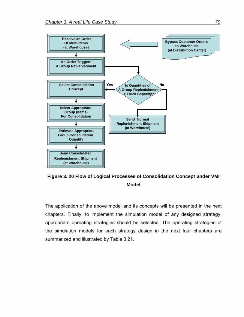
Chapter 3. A real Life Case Study 79
Select Appropriate Group (items)
For Consolidation
Bypass Customer Orders to Warehouse
(at Distribution Center)
Receive an OrderOf Multi-Items
(at Warehouse)
An Order Triggers A Group Replenishment
Select ConsolidationConcept
Estimate AppropriateGroup Consolidation
Quantity
Send Consolidated Replenishment Shipment
(at Warehouse)
Is Quantities of A Group Replenishment
< Truck Capacity?
Yes No
Send NormalReplenishment Shipment
(at Warehouse)
Figure 3. 20 Flow of Logical Processes of Consolidation Concept under VMI Model
The application of the above model and its concepts will be presented in the next
chapters. Finally, to implement the simulation model of any designed strategy,
appropriate operating strategies should be selected. The operating strategies of
the simulation models for each strategy design in the next four chapters are
summarized and illustrated by Table 3.21.

Chapter 3. A real Life Case Study 80
Table 3. 21 Operating Strategies of the Simulation Model
Operating Strategy UCS CS UCS-V CS-V
with Allowed to
keep inventory
X
X
In
vent
ory
Pol
icy
Not allowed to
keep inventory
X
X
FTL Concept
(Consolidation
Concepts)
X
X
Rep
leni
shm
ent
Pol
icy
LTL Concept
(Only
Demanded
Order)
X
X
UCS: Uncoordinated Strategy
CS: Coordination Strategy
UCS-V: Uncoordinated Strategy with VMI approach
CS-V: Coordination Strategy with VMI approach
FTL: Full Truckload
LTL: Less than Truckload.
Chapter 4.Uncoordinated Distribution Strategies 81
4. Design and Analysis of Uncoordinated Distribution Strategies:
Item Classification approaches
The aim of this chapter is to show the sensitivity of distribution strategies in supply
chains to item classification approaches and to show the difficulties of optimizing
such complex systems, due to the conflicts of system objectives. To achieve the
aim, the developed simulation model is used and implemented.
4.1. ABC Classification, XYZ, and ABC-XYZ Classification approaches
In multi-item inventory systems, classification of inventories can help to reduce the
complexity of managing thousands of items. Many researchers [FW87] recommend
the use of a two dimensional classification systems, where the first is the traditional
ABC classification and the second is based on criticality. In this thesis a two
dimensional classification of items is used. The first is the traditional ABC
classification and the second is based on variability (XYZ classification).
4.1.1. ABC Classification
ABC classification is a practical approach [EB94], [Bal04], [SKS03] applied for
multi-item inventory problems. Different item classifications need different
replenishment and inventory control policies. Different types of items also need
different ways of replenishment. Silver et al. [SPP98] propose the so-called ABC-
classification, based on the perception that items with a large turnover (A-items)
need to be controlled differently compared with items with a low turnover (C-items).
In this classification approach, the items are classified based on demand
(consumption) rate:

Chapter 4.Uncoordinated Distribution Strategies 82
● A-Class: This class represents about 11 to 24% of the items carried in
inventory and 75% of the consumption rate (fast-moving items).
● B-Class: This class represents about 13 to 23% of the items carried in
inventory and 15% of the consumption rate.
● C-Class: This class represents about 55 to 75% of the items carried in
inventory and 10% of the consumption rate (slow-moving items).
The classification has been done for all the distribution centers based on the real
demand data from the company. The ABC classification of some distribution
centers are illustrated in the following figures:
0%
10%
20%
30%
40%
50%
60%
70%
80%
90%
100%
110%
1,14
%
6,82
%
12,5
0%
18,1
8%
23,8
6%
29,5
5%
35,2
3%
40,9
1%
46,5
9%
52,2
7%
57,9
5%
63,6
4%
69,3
2%
75,0
0%
80,6
8%
86,3
6%
92,0
5%
97,7
3%
Item Percentage
Con
sum
ptio
n R
ate(
%)
CA B
Figure 4. 1 ABC Classification for LDC1

Chapter 4.Uncoordinated Distribution Strategies 83
0%
10%
20%
30%
40%
50%
60%
70%
80%
90%
100%
110%
1,09
%
6,52
%
11,9
6%
17,3
9%
22,8
3%
28,2
6%
33,7
0%
39,1
3%
44,5
7%
50,0
0%
55,4
3%
60,8
7%
66,3
0%
71,7
4%
77,1
7%
82,6
1%
88,0
4%
93,4
8%
98,9
1%
Item Percentage
Con
sum
ptio
n R
ate(
%)
CA B
Figure 4. 2 ABC Classification for LDC5
0%
10%
20%
30%
40%
50%
60%
70%
80%
90%
100%
110%
0,89
%
5,36
%
9,82
%
14,2
9%
18,7
5%
23,2
1%
27,6
8%
32,1
4%
36,6
1%
41,0
7%
45,5
4%
50,0
0%
54,4
6%
58,9
3%
63,3
9%
67,8
6%
72,3
2%
76,7
9%
81,2
5%
85,7
1%
90,1
8%
94,6
4%
99,1
1%
Item Percentage
Con
sum
ptio
n R
ate(
%)
CA B
Figure 4. 3 ABC Classification for RDC15

Chapter 4.Uncoordinated Distribution Strategies 84
0%
10%
20%
30%
40%
50%
60%
70%
80%
90%
100%
110%
0,92
%
5,50
%
10,0
9%
14,6
8%
19,2
7%
23,8
5%
28,4
4%
33,0
3%
37,6
1%
42,2
0%
46,7
9%
51,3
8%
55,9
6%
60,5
5%
65,1
4%
69,7
2%
74,3
1%
78,9
0%
83,4
9%
88,0
7%
92,6
6%
97,2
5%
Item Percentage
Con
sum
ptio
n R
ate(
%)
CA B
Figure 4. 4 ABC Classification for RDC19
Table 4.1 shows the percentage of items in each class for each distribution centre
and Figure 4.5 shows the average percentage of items in each class for all the
distribution centers.

Chapter 4.Uncoordinated Distribution Strategies 85
Table 4. 1 Percentage of Items in each Class for each Distribution Center
19,41%
18,03%62,55%
A B C
Figure 4. 5 Average Percentages of Items in each Class
D C A B C TotalR D C 1 20,75% 19,81% 59,43% 100,00%R D C 2 17,59% 19,44% 62,96% 100,00%R D C 3 15,93% 18,58% 65,49% 100,00%R D C 4 22,12% 19,23% 58,65% 100,00%R D C 5 14,55% 17,27% 68,18% 100,00%R D C 6 12,69% 17,91% 69,40% 100,00%R D C 7 20,18% 15,79% 64,04% 100,00%R D C 8 15,60% 17,43% 66,97% 100,00%R D C 9 11,11% 19,44% 69,44% 100,00%
R D C 10 24,55% 16,36% 59,09% 100,00%R D C 11 19,27% 17,43% 63,30% 100,00%R D C 12 24,30% 20,56% 55,14% 100,00%R D C 13 23,89% 17,70% 58,41% 100,00%R D C 14 15,65% 22,61% 61,74% 100,00%R D C 15 11,61% 13,39% 75,00% 100,00%R D C 16 12,50% 18,27% 69,23% 100,00%R D C 17 21,60% 15,20% 63,20% 100,00%R D C 18 21,50% 22,43% 56,07% 100,00%R D C 19 18,35% 21,10% 60,55% 100,00%LD C 1 22,73% 17,05% 60,23% 100,00%LD C 2 23,26% 15,12% 61,63% 100,00%LD C 3 18,29% 15,85% 65,85% 100,00%LD C 4 29,63% 18,52% 51,85% 100,00%LD C 5 28,26% 16,30% 55,43% 100,00%

Chapter 4.Uncoordinated Distribution Strategies 86
4.1.2. XYZ Classification:
The variability of item demand (consumption) must be taken into consideration in
order to improve the supply chain processes [Sch01], [RT02], [Knu03]. The items
are classified based on demand variability. The variability is measured by the
coefficient of variation (CV), the standard deviation of daily demand divided by the
mean.
● X-Class: In this class daily demand variability is low (CV ≤ 0.5).
● Y-Class: In this class daily demand variability is intermediate (0.5< CV ≤ 1.0).
● Z-Class: In this class daily demand variability is high (CV > 1.0).
For an item with very low coefficient of variation, the demand can be forecasted
with good accuracy. For an item with very high coefficient of variation, the demand
can not be forecasted with accuracy.
As in the first classification, the XYZ classification has been done for all the
distribution centers based on the real demand data from the company. The XYZ
classification of some distribution centers are exhibited in the following figures.

Chapter 4.Uncoordinated Distribution Strategies 87
0
0,5
1
1,5
2
2,5
3
3,5
1,14
%
6,82
%
12,5
0%
18,1
8%
23,8
6%
29,5
5%
35,2
3%
40,9
1%
46,5
9%
52,2
7%
57,9
5%
63,6
4%
69,3
2%
75,0
0%
80,6
8%
86,3
6%
92,0
5%
97,7
3%
Item Percentage
CV
X Y Z
Figure 4. 6 XYZ Classification for LDC1
0
0,5
1
1,5
2
2,5
3
3,5
4
4,5
1,09
%
6,52
%
11,9
6%
17,3
9%
22,8
3%
28,2
6%
33,7
0%
39,1
3%
44,5
7%
50,0
0%
55,4
3%
60,8
7%
66,3
0%
71,7
4%
77,1
7%
82,6
1%
88,0
4%
93,4
8%
98,9
1%
Item Percentage
CV
X Y Z
Figure 4. 7 XYZ Classification for LDC5

Chapter 4.Uncoordinated Distribution Strategies 88
0
0,5
1
1,5
2
2,5
3
0,89
%
5,36
%
9,82
%
14,2
9%
18,7
5%
23,2
1%
27,6
8%
32,1
4%
36,6
1%
41,0
7%
45,5
4%
50,0
0%
54,4
6%
58,9
3%
63,3
9%
67,8
6%
72,3
2%
76,7
9%
81,2
5%
85,7
1%
90,1
8%
94,6
4%
99,1
1%
Item Percentage
CV
X Y Z
Figure 4. 8 XYZ Classification for RDC15
0
0,5
1
1,5
2
2,5
3
3,5
4
0,92
%
5,50
%
10,0
9%
14,6
8%
19,2
7%
23,8
5%
28,4
4%
33,0
3%
37,6
1%
42,2
0%
46,7
9%
51,3
8%
55,9
6%
60,5
5%
65,1
4%
69,7
2%
74,3
1%
78,9
0%
83,4
9%
88,0
7%
92,6
6%
97,2
5%
Item Percentage
CV
X Y Z
Figure 4. 9 XYZ Classification for RDC19

Chapter 4.Uncoordinated Distribution Strategies 89
The percentage of items in each class for each distribution center is shown in
Table 4.2 and the average percentage of items in each class for all the distribution
centers is illustrated by Figure 4.10.
Table 4. 2 Percentage of Items in each Class for each Distribution Center
19,14%
49,68%
31,18%
X Y Z
Figure 4. 10 Average Percentages of Items in each Class
D C X Y Z T o ta lR D C 1 1 6 ,0 4 % 4 8 ,1 1 % 3 5 ,8 5 % 1 0 0 ,0 0 %R D C 2 2 5 ,9 3 % 4 0 ,7 4 % 3 3 ,3 3 % 1 0 0 ,0 0 %R D C 3 1 8 ,5 8 % 5 3 ,1 0 % 2 8 ,3 2 % 1 0 0 ,0 0 %R D C 4 2 2 ,1 2 % 5 6 ,7 3 % 2 1 ,1 5 % 1 0 0 ,0 0 %R D C 5 1 9 ,0 9 % 5 1 ,8 2 % 2 9 ,0 9 % 1 0 0 ,0 0 %R D C 6 8 ,9 6 % 5 1 ,4 9 % 3 9 ,5 5 % 1 0 0 ,0 0 %R D C 7 1 1 ,4 0 % 4 5 ,6 1 % 4 2 ,9 8 % 1 0 0 ,0 0 %R D C 8 1 0 ,0 9 % 4 8 ,6 2 % 4 1 ,2 8 % 1 0 0 ,0 0 %R D C 9 2 9 ,6 3 % 4 7 ,2 2 % 2 3 ,1 5 % 1 0 0 ,0 0 %
R D C 1 0 2 3 ,6 4 % 4 5 ,4 5 % 3 0 ,9 1 % 1 0 0 ,0 0 %R D C 1 1 1 7 ,4 3 % 5 8 ,7 2 % 2 3 ,8 5 % 1 0 0 ,0 0 %R D C 1 2 3 ,7 4 % 5 7 ,9 4 % 3 8 ,3 2 % 1 0 0 ,0 0 %R D C 1 3 1 9 ,4 7 % 4 9 ,5 6 % 3 0 ,9 7 % 1 0 0 ,0 0 %R D C 1 4 2 5 ,2 2 % 4 7 ,8 3 % 2 6 ,9 6 % 1 0 0 ,0 0 %R D C 1 5 9 ,8 2 % 4 8 ,2 1 % 4 1 ,9 6 % 1 0 0 ,0 0 %R D C 1 6 2 2 ,1 2 % 3 5 ,5 8 % 4 2 ,3 1 % 1 0 0 ,0 0 %R D C 1 7 2 1 ,6 0 % 3 8 ,4 0 % 4 0 ,0 0 % 1 0 0 ,0 0 %R D C 1 8 1 ,8 7 % 4 5 ,7 9 % 5 2 ,3 4 % 1 0 0 ,0 0 %R D C 1 9 5 ,5 0 % 4 4 ,0 4 % 5 0 ,4 6 % 1 0 0 ,0 0 %L D C 1 2 3 ,8 6 % 6 5 ,9 1 % 1 0 ,2 3 % 1 0 0 ,0 0 %L D C 2 3 1 ,4 0 % 5 0 ,0 0 % 1 8 ,6 0 % 1 0 0 ,0 0 %L D C 3 2 4 ,3 9 % 5 2 ,4 4 % 2 3 ,1 7 % 1 0 0 ,0 0 %L D C 4 3 7 ,0 4 % 5 8 ,0 2 % 4 ,9 4 % 1 0 0 ,0 0 %L D C 5 3 0 ,4 3 % 5 1 ,0 9 % 1 8 ,4 8 % 1 0 0 ,0 0 %

Chapter 4.Uncoordinated Distribution Strategies 90
ABC-XYZ Classification
To get more insight into the behavior and sensitivity of the demand pattern of each
item, the items are clustered or grouped based on the combination of two
classifications (ABC & XYZ classifications). Nine different categories (classes) of
items are generated (XA, XB, XC, YA, YB, YC, ZA, ZB, and ZC). Figure 4.11
shows the percentage of items in the nine classes for each distribution center.
Figure 4.12 illustrates the average percentage of items in each class for all the
distribution centers.
0%
10%
20%
30%
40%
50%
60%
70%
80%
90%
100%
RDC1RDC2
RDC3RDC4
RDC5RDC6
RDC7RDC8
RDC9
RDC10
RDC11
RDC12
RDC13
RDC14
RDC15
RDC16
RDC17
RDC18
RDC19LD
C1LD
C2LD
C3LD
C4LD
C5
XA XB XC YA YB YC ZA ZB ZC
Figure 4. 11 Percentage of Items in each Class for each Distribution Center

Chapter 4.Uncoordinated Distribution Strategies 91
7,80%5,61%
5,74%
9,51%
8,51%
31,67%
2,11%3,92%
25,15%
XA XB XC YA YB YC ZA ZB ZC
Figure 4. 12 Average Percentages of Items in each Class
Classification of items can also help to design more appropriate distribution
strategies based on the objectives of supply chain decision makers. This fact has
been proven by designing a lot of distribution strategies, using a two classification
approach to achieve some goals and then comparing the results with those from
some common strategies. As seen in the previous figures and tables, the item
percentage of each class for each distribution center is completely different as
compared with another distribution center for each of the three classification
approaches (Table 4.1, 4.2, and Figure 4.11). Therefore, using a common
distribution strategy for all the distribution centers based on the item classification
is very difficult and hence the comparison is more complex. All of these difficulties
and the design of the distribution strategies are described and discussed in the
following sections.

Chapter 4.Uncoordinated Distribution Strategies 92
4.2. Design of Uncoordinated Strategy Experiments
The design of each experiment strategy is constructed mainly based on the
following four control parameters:
1. ABC classification
2. XYZ classification
3. Reorder point (fixed for each class or individual based on service level, s).
4. Maximum inventory level (order up-to-level, S).
For designing these experiments, some assumptions are considered:
• In all experiments the beginning inventory is assumed to be equal to the
reorder point and the lead time is four days (LT = 4 Days).
• The inventory decisions are taken at the distribution centers.
• The continuous review installation stock (s, S) policy where s is the reorder
point and S is the order up-to-level is used as inventory policy for all the
experiments.
• The physical maximum capacity of inventory levels should be limited.
• The customer orders are filled completely.
• The filling of customer orders is based on a first-in-first-out (FIFO) rule.
• The number of distribution centers that have been considered is twenty four
(DC's = 24).
Notation:
UCS-Expt: uncoordinated Strategy experiment
By using the above parameters and assumptions, ten experiments are constructed.
The ten experiments are conducted by implementing the simulation model
described in chapter three. To conduct the experiments by using the developed
simulation model, the user should select the appropriate inventory policy and
replenishment policy for each location in the network. In these experiments, the

Chapter 4.Uncoordinated Distribution Strategies 93
downstream locations were selected as the “distribution centres” for location type
and “Allowed to keep inventory” was selected as the inventory policy. In this case,
the distribution centres function as traditional stores and all the inventory decisions
are taken at downstream locations (DCs). The less-than-truck-load (LTL) is also
selected as the transportation strategy by selecting the (Only Demanded Order
replenishment) as the replenishment policy. All of these strategies and policies
could be selected through the input data mask parameters (Figure 3.5 and 3.19).
As mentioned above, the (s, S) system is used as a policy for controlling the
inventory. It is interesting that (s, S) systems are frequently encountered in
practice. However, the values of the control parameters are usually set in a rather
arbitrary fashion. For B items (and even most A items) mathematical optimality
does not make sense; instead, a fairly simple way of obtaining reasonable values
of s and S is needed [SPP98]. Therefore, in the following experiments the values of
s and S parameters for each item type are estimated by different ways to see the
effect of selecting these control parameters on the performance of distribution
strategies and also to see the benefit of using the simulation as a tool for
estimating the optimal value of such parameters.
4.2.1. Experiment ABC– Item Strategy (without Safety Stock) - (UCS- Expt 1):
In this experiment only three of the above parameters have been considered.
These parameters are the ABC classification, the reorder point and the maximum
inventory level. The reorder point of each item is designed mainly based on
common inventory policy (equal to the average demand during the lead time). The
reorder point and the maximum inventory level of each item type are estimated by
the following formulas:
Reorder Point (s) = Lead Time * Average Demand (Daily) (4.1)

Chapter 4.Uncoordinated Distribution Strategies 94
Maximum Inventory Level (S) = Number of Days * Average Demand (Daily) (4.2)
The design of the experiment is summarized as shown in Table 4.3:
Table 4. 3 Reorder Point and Maximum Inventory Level for Each Item Class
The above maximum inventory level is designed by taking the physical maximum
capacity of the distribution centers in to consideration.
4.2.2. Experiment ABC-Item Strategy (with Safety Stock) – (UCS-
Expt 2):
This experiment is designed in the same manner as the previous experiment
except that the safety stock is considered in a different way. In this case the safety
stock is equal to the fifty percentage of the demand during lead time [Bal04].
The reorder point of each item is designed as given by the following formula:
Reorder Point (s) = Lead Time * Average Demand (Daily) + Safety Stock
Reorder Point (s) = Lead Time * Average Demand (Daily) + 50% of [Lead Time * Average Demand (Daily)] (4.3)
Maximum inventory level (S) of each item is calculated by equation (4.2). The
design of the experiment is summarized in Table 4.4:
ABC Classification s (Days) S (Days)A 4 10B 4 10C 4 15

Chapter 4.Uncoordinated Distribution Strategies 95
Table 4. 4 Reorder Point and Maximum Inventory Level for Each Item Class
4.2.3. Experiment ABC- Item Strategy (minimize transportation) – (UCS- Expt 3):
This strategy is designed mainly to get more savings on transportation costs. Due
to attractive transportation cost rate with increased quantity, the shipment size of
high consumption rate or important items (A items) is large and that for B- and C-
items is lower. Most companies also keep a relatively large number of units of low
consumption or important items (C items) in stock to minimize the amount of
inconvenience that could be caused by a stockout of such insignificant parts
[SPP98].
Based on all the mentioned rules, the reorder point and the maximum inventory
level of each item are designed by selecting the appropriate number of days. It is
clear that the difference in days between the s and S values determine the
shipment size. Therefore, for example, to generate a large shipment size of type A-
items, the difference between the s and S in days should be big. For keeping a
large number of the type C-items at the distribution centers, the number of days for
estimating the reorder point of such item type should be high.
The reorder point and maximum inventory level of each item are estimated by the
general equation (4.4). Table 4.5 illustrates the number of days given for each
parameter.
s or S = Number of Days * Average Demand (Daily) (4.4)
ABC Classification s (Days) S (Days)A 6 10B 6 10C 6 15

Chapter 4.Uncoordinated Distribution Strategies 96
Table 4. 5 Reorder Point and Maximum Inventory Level for Each Item Class
4.2.4. Experiment C- Item Allocation Strategy- (UCS- Expt 4):
The allocation of item inventory is one of the distribution strategies which has been
widely used in the literatures and practice to minimize the systemwide cost
especially when the holding cost is very high [NT01], [CM04]. Additionally, other
factors, such as the emergency of items and the satisfaction of customers, should
be considered. All of these savings and the factors will be realised by this
experiment. The logic of this strategy is to keep items with a very low demand or
slow-moving items (C) at upstream location (Warehouse) and items with a very
high demand or fast-moving items or more demanded items (A and B) close to the
customer, at the lowest downstream location (Distribution Centre) to minimize the
inventory and transportation costs. By using the equation (4.4) the reorder point
and maximum level of each item are constructed. To implement this strategy, the
reorder point (s) for each type C-item is estimated as zero days. Table 4.6 shows
the design of the strategy:
Table 4. 6 Reorder Point and Maximum Inventory Level for Each Item Class
ABC Classification s (Days) S (Days)A 4 10B 6 10C 10 15
ABC Classification s (Days) S (Days)A 4 10B 4 10C 0 15

Chapter 4.Uncoordinated Distribution Strategies 97
4.2.5. Experiment XYZ-Item Strategy - (UCS- Expt 5):
The uncertainty in the demand pattern of multi items significantly complicates the
controlling of the inventory and the designing of an appropriate distribution
strategy. Most organizations make an appropriate reallocation of safety stock to
meet the unexpected fluctuations in demand which lead to a significant
improvement in the customer services. More safety stocks should be given for
items with high variability demand and vice versa. The two parameters (s & S) are
designed by taking the uncertainty into account and by calculating using the same
equation (4.4). For example, the value of the reorder point (s) for the high variability
items (Z) is the biggest. Table 4.7 shows the estimation of these two parameters (s
& S).
Table 4. 7 Reorder Point and Maximum Inventory Level for Each Item Class
4.2.6. Experiment Z- Item Allocation Strategy- (UCS- Expt 6):
In this experiment, the logic of the strategy is to keep the items with high variability
demand (Z Item), that are very difficult to be forecasted, at the upstream location
(Warehouse) and the items with low variability demand, that can be forecasted with
accuracy, close to the customer at lowest downstream location (Distribution
Centre).Therefore, the reorder point for each type Z-item is estimated to be zero
days. The reorder point and maximum inventory level of each item type are
estimated by equation (4.4).
The strategy is designed as given in Table 4.8.
XYZ Classification s (Days) S (Days)X 4 10Y 6 10Z 10 15

Chapter 4.Uncoordinated Distribution Strategies 98
Table 4. 8 Reorder Point and Maximum Inventory Level for Each Item Class
4.2.7. Experiment ABC- XYZ - Combination Strategy- (UCS- Expt 7):
In this experiment, nine classes of items are generated based on the ABC-XYZ
classification. The reorder point of each item is constructed based on these nine
categories and by using equation (4.4). The mechanism of this strategy is to give
more safety stock for a very important item with high variability demand (YA, ZA,
and ZB) and less safety stocks for less important item with high demand variability
(YC and ZC). For example, the value of s for the type ZA-item is the largest and for
the type ZC-item is the smallest.
The reorder point is given by Table 4.9:
Table 4. 9 Reorder Point for Each Combined Item Class
The maximum inventory level is given in Table 4.10:
Table 4. 10 Maximum Inventory Level for Each Combined Item Class
Note: all the values in the tables are in days.
A B CX 4 4 4Y 5 4 2Z 6 5 1
A B CX 10 10 15Y 10 10 15Z 10 10 15
XYZ Classification s (Days) S (Days)X 4 10Y 4 10Z 0 15

Chapter 4.Uncoordinated Distribution Strategies 99
4.2.8. Experiment ABC- XYZ – Combination Strategy (MIL) - (UCS- Expt 8):
This experiment is designed by the same method as that used in the previous
combination experiment. The only difference is in the maximum level estimation.
Here the maximum level of less important items (B and C) is reduced to minimize
the shipment size and the average ending inventory of these items. For example,
in all the previous experiments the value of the maximum inventory level (S) of the
type C-items is equal to fifteen days, and in this strategy it is only eight days.
The maximum inventory level is given by Table 4.11:
Table 4. 11 Maximum Inventory Level for Each Combined Item Class
Note: all the values in the tables are in days.
4.2.9. Experiment CSL (80%) ABC Item Strategy- (UCS- Expt 9):
As the variability of demand grows the required level of safety stock inventory
increases. The appropriate level of safety stock inventory is determined by the
following two factors [CM04]:
1. The uncertainty of both demand and supply
2. The desired level of product availability
One of the measures of item availability is Cycle Service Level (CSL).
Cycle Service Level (CSL) is the fraction of replenishment cycles that end with all
the customer demand being met. A replenishment cycle is the interval between two
successive replenishment deliveries. Therefore, CSL is equal to the probability of
not having a stockout in a replenishment cycle. In this case safety stock (safety
A B CX 10 8 8Y 10 8 8Z 10 8 8

Chapter 4.Uncoordinated Distribution Strategies 100
inventory) is determined based on desired Cycle Service Level (CSL) of decision
makers. The reorder point (s) for each item will be calculated based on this result.
The procedure can be described as follows:
Observe that a stockout occurs in a cycle if demand during the lead time is larger
than the ROP (s). Thus, identify the safety inventory SS such that the following is
true:
CSL= probability (demand during lead time ≤ SSDL + )
• If demand during lead time is normally distributed with a mean of LD and a
standard deviation of Lσ where,
LDDL ×= and DL L σσ ×= , so that
CSLDSSDF LLL =+ ),,( σ (4.5)
• By using the definition of the inverse normal, the equation can be derived
),,(1LLL DCSLFSSD σ−=+ , or LLL DDCSLFSS −= − ),,(1 σ (4.6)
• By using the definition of standard normal distribution, its inverse can be
modified as follows:
LS CSLFSS σ×= − )(1 (4.7)
Finally, the reorder point (s) can be calculated by
SSDs L += (4.8)
where:
=CSL Desired cycle service level,
=D Average demand,

Chapter 4.Uncoordinated Distribution Strategies 101
=Dσ Standard deviation of demand,
=LD Mean demand during lead time,
=Lσ Standard deviation of demand during lead time,
=L Average lead time for replenishment
=SS Safety stock
=s Reorder point
This procedure has been applied under an important assumption that the
continuous review replenishment (ROP, Q) policy is implemented. In this thesis the
procedure is used under (s, S) replenishment policy and with different distributions
of the demand and lead time.
In this experiment, the reorder point of each item is designed to achieve a CSL of
80%. The maximum inventory level of each item is calculated as in the previous
experiments. The reorder point designed of each item is calculated by equation
(4.8) and the maximum inventory level of each class is calculated by equation
(4.4). Table 4.12 shows the desired Cycle Service Level (CSL) and the maximum
inventory level for each item class:
Table 4. 12 Cycle Service Level and Maximum Inventory Level for Each Item Class
4.2.10. Experiment CSL (90%) ABC Item Strategy- (UCS-Expt 10):
The reorder point and the maximum inventory of each item are estimated using the
same procedures in the previous strategy; here the reorder point of each item is
designed to achieve a CSL of 90 percent.
ABC Classification CSL(%) S (Days)A 80% 10B 80% 10C 80% 15

Chapter 4.Uncoordinated Distribution Strategies 102
The designed parameters of this experiment are shown in Table 4.13.
Table 4. 13 Cycle Service Level and Maximum Inventory Level for Each Item Class
The design of all the ten strategies will be summarized in the following tables:
Table 4. 14 Experimental Index (1)
Table 4. 15 Experimental Index (2)
Table 4. 16 Experimental Index (3)
ABC Classification CSL(%) S (Days)A 90% 10B 90% 10C 90% 15
A B C X Y Z A B C X Y ZUCS- Expt 1 4 4 4 - - - 10 10 15 - - -UCS- Expt 2 6 6 6 - - - 10 10 15 - - -UCS- Expt 3 4 6 10 - - - 10 10 15 - - -UCS- Expt 4 4 4 0 - - - 10 10 15 - - -UCS- Expt 5 - - - 4 6 10 - - - 10 10 15UCS- Expt 6 - - - 4 4 0 - - - 10 10 15
Expt-Names (Days) S (Days)
A B C X Y Z A B C X Y ZUCS- Expt 9 80% 80% 80% - - - 10 10 15 - - -UCS- Expt 10 90% 90% 90% - - - 10 10 15 - - -
Expt-NameCSL (%) S (Days)
XA XB XC YA YB YC ZA ZB ZC XA XB XC YA YB YC ZA ZB ZCUCS- Expt 7 4 4 4 5 4 2 6 5 1 10 10 15 10 10 15 10 10 15UCS- Expt 8 4 4 4 5 4 2 6 5 1 10 8 8 10 8 8 10 8 8
s (Days) S (Days)Expt-Name

Chapter 4.Uncoordinated Distribution Strategies 103
4.3. Performance Measures:
To compare the experiments and to see how significantly each the strategies
affects the system performance, six measures of performance are selected to
provide measures of the logistics costs and customer responsiveness/ backorders.
These measures are most commonly used to measure the supply chain
performance, and are described in the following section:
In the following sections the following notations are used:
=i Distribution centre i .
=I Total number of items
=j Warehouse j
=TC Transportation cost for one year
=n Total number of distribution centres
=W Total number of warehouses
=s A stockout item
=S Total number of stockout items
=sc A stockout item in a class
=C Total number of stockout items in a class
4.3.1. Total Transportation Cost (TTC):
This is equal to the sum of the transportation costs for one year between each
warehouse and distribution centre (Inbound Transportation cost). The required
data for calculating TTC is collected from the financial summary report (Table 3.10
and Table 3.14).
TTC = ∑∑= =
W
jji
n
iTC
1 1, (4.9)
Where jiTC is the transportation cost between warehouse j and distribution centre i.

Chapter 4.Uncoordinated Distribution Strategies 104
4.3.2. Total Inventory Holding Cost (TIHC):
This is equal to the sum of the inventory holding costs for one year for all
distribution centres. It is calculated using the average daily ending inventory (pallet
unit). To calculate the average daily ending inventory, some data should be
collected from aggregated inventory investment report (Table 3.12).
TIHC = ∑=
n
iiIHC
1
(4.10)
=IHC Inventory holding cost for one year.
4.3.3. Total Logistics Cost (TLC):
This is equal to the sum of the transportation cost and inventory holding cost.
TLC = TTC + TIHC (4.11)
4.3.4. Item Fill Rate Measures:
This is the fraction of item demand that is satisfied from item stock.
1. Item Fill Rate (IFR) = 1 - (total number of orders of an item not satisfied /total
number of orders of an item) (4.12)
2. Average Item Fill Rate of each DC (AIFR) = S
IFRS
ss∑
=1)(
(4.13)
3. Average Item Fill Rate of each Class (AIFRC) = C
IFRC
scsc∑
=1)(
(4.14)
4. Average of Average Item Fill Rate of all DCs (AAIFR) =n
AIFRn
ii∑
=1)(
(4.15)

Chapter 4.Uncoordinated Distribution Strategies 105
4.3.5. Order Lines Fill Rate Measures:
The order line fill rate is the fraction of order lines that is satisfied immediately from
item stock.
Order Lines Fill Rate of each DC (OLFR):
linesorderofnumberTotalsatisfiednotlinesorderofnumberTotalOLFR −= 1 (4.16)
Average of Order Lines Fill Rate of all DCs (AOLFR):
DCsofnumberTotalDCsofratefilllinesorderTotalAOLFR =
n
OLFRAOLFR
n
ii∑
== 1)(
(4.17)
For calculating OLFR and IFR, some data from inventory tracing reports should be
collected (Table 3.11).
4.3.6. Order Fill Rate Measures:
The order fill rate is the fraction of orders that are filled completely from available
item stock. This measure is very important when the customer orders must be filled
completely.
The Order Fill Rate of each DC (OFR):
ordersofnumberTotalsatisfiednotorderofnumberTotalOFR −= 1 (4.18)
Average of Order Fill Rate (AOFR):

Chapter 4.Uncoordinated Distribution Strategies 106
DCsofnumberTotalDCsofratefillorderTotalAOFR =
n
OFRAOFR
n
ii∑
== 1 (4.19)
The required data for calculating OFR is gathered from service order degree
reports (Table 3.16).
Some costs (Pickup, Order, unloading, and loading) are negligible compared with
transportation or holding costs, so for the sake of simplicity they are not taken into
account.
4.4. Experimental Simulation Results and Analysis
Simulation results are collected after running the simulation model for one year.
Once the model has been simulated, many detailed output reports on every aspect
of the measures of performance are generated by the simulation model (see
chapter three). The simulation results (measures of performance), analysis of
results and some findings will be shown in the following section.
The summary of measures of performance for each strategy are ranked in
ascending order based on the average order fill rate (AOFR) and presented in
Table 4.17 and Figure 4.13. Figure 4.14 shows the percentage increase in the total
logistics costs for each strategy as compared with the experiment C-Item Allocation
Strategy. This strategy (UCS- Expt 4) has been considered as a base experiment
because it has the minimum total logistics costs.

Chapter 4.Uncoordinated Distribution Strategies 107
Table 4. 17 Measures of Performance for Each Strategy Based on Ascending Order of Average Order Fill Rate
Experiments TTC TIHC TLC AOLFR AOFRUCS-Expt 4* $8.109.584,95 $205.694,79 $8.315.279,74 86,49% 10,10%UCS-Expt 6 $8.116.662,30 $233.927,36 $8.350.589,66 88,91% 12,98%UCS-Expt 8 $8.146.816,06 $238.005,21 $8.384.821,27 92,06% 32,76%UCS-Expt 7 $8.124.646,65 $266.363,19 $8.391.009,84 95,04% 43,23%UCS-Expt 1 $8.114.944,57 $276.000,10 $8.390.944,67 96,44% 61,06%UCS-Expt 5 $8.139.476,97 $340.781,80 $8.480.258,77 97,44% 71,46%UCS-Expt 3 $8.125.338,06 $344.206,49 $8.469.544,55 98,17% 77,19%UCS-Expt 9 $8.139.772,59 $317.015,50 $8.456.788,09 98,23% 78,45%UCS-Expt 2 $8.149.488,60 $321.158,15 $8.470.646,75 98,68% 83,65%UCS-Expt 10 $8.150.344,06 $340.914,26 $8.491.258,32 98,72% 84,08%
* Base Experiment
10,10%12,98%
32,76%
43,23%
61,06%
71,46%77,19% 78,45%
83,65%84,08%
7,90E+06
8,00E+06
8,10E+06
8,20E+06
8,30E+06
8,40E+06
8,50E+06
8,60E+06
UCS-Exp
t 4*
UCS-Exp
t 6
UCS-Exp
t 8
UCS-Exp
t 7
UCS-Exp
t 1
UCS-Exp
t 5
UCS-Exp
t 3
UCS-Exp
t 9
UCS-Exp
t 2
UCS-Exp
t 10
Experiments
Cos
ts ($
)
0%
20%
40%
60%
80%
100%
120%
Fill
Rat
e
TTC TLC AOLFR AOFR
Figure 4. 13 Measures of Performance for Each Strategy Based on Ascending Order of Average Order Fill Rate

Chapter 4.Uncoordinated Distribution Strategies 108
0,00%
0,42%
0,84%0,91%
1,70%
1,87%1,98%
2,12%
0,91%
1,86%
0,00%
0,50%
1,00%
1,50%
2,00%
2,50%
UCS-Exp
t 4*
UCS-Exp
t 6
UCS-Exp
t 8
UCS-Exp
t 1
UCS-Exp
t 7
UCS-Exp
t 9
UCS-Exp
t 3
UCS-Exp
t 2
UCS-Exp
t 5
UCS-Exp
t 10
Experiments
Incr
easi
ng T
LC
Figure 4. 14 Percentage Increase of the Total Logistics Costs
4.4.1. Logistics Costs Analysis:
The following analysis can be made based on Table 4.17 and Figure 4.13:
1. In the case minimizing of the total logistic cost is the main objective and if
the item fill rate is not to be less than 85% and that it is not used as a
measure of performance (especially when the holding inventory cost is very
high and the customer orders are partially filled) then it is recommended that
allocation strategies are used.
2. From the results, the C-Item allocation strategy performs better than the Z-
Item allocation strategy and the reduction of the total logistic cost is about
more than 0.5% but the Z-Item has improved the fill rate by more than 2%.
This can be explained by the fact that the keeping of slow-moving items (C)
at upstream location produces less transportation between the upstream
and downstream locations as compared with keeping the Z items at

Chapter 4.Uncoordinated Distribution Strategies 109
upstream locations. Keeping the Z items at upstream locations produces
more transportation because some of Z items are A items (fast-moving
items) which are more demanded items. Also, keeping slow-moving items
(C) at upstream locations produces less ending inventory at the downstream
locations as compared with keeping the Z items at upstream locations. This
is due to the difference in the item percentage of each class. The average
item percentage of C items class is equal to 62.55% and the average item
percentage of the Z items class is equal to 31.18% (Table 4.1, Table 4.2,
Figure 4.5, and Figure 4.10). Furthermore, the significant difference in item
percentages justifies, in general, the low average order fill rate for both
strategies.
3. In the case where the inventory levels are adjusted to achieve an item fill
rate of more than 90%, 70% order fill rate and transportation costs have the
first priority, it is recommended to use experiment ABC-item strategy. It
performs better than the others with a saving in transportation cost of 0.30%.
4. In the case where the order fill rate (more than 80%) has the first priority, it
is recommended to use the common strategies, especially the CLS-
Strategies. These strategies are more sensitive to item variability and
therefore they can produce high service levels with no considerable increase
in the total logistics costs.
5. In most cases, as the order fill rate is increased the total logistics costs are
increased.
6. On the other hand, a high average daily ending inventory (TIHC) cannot be
correlated with the high service levels (AOLFR & AOFR) in all the strategies.
For example, the experiment CSL (90%) ABC Item strategy (UCS-Expt 10)
and the experiment XYZ-Item strategy (UCS- Expt 5) have approximately
the same total inventory holding cost (TIHC), but the AOFR of the UCS-Expt
10 strategy is approximately 13% higher than that in the UCS- Expt 5
strategy.

Chapter 4.Uncoordinated Distribution Strategies 110
7. As seen in Figure 4.14, the optimal strategy (Experiment CSL (90%) ABC
Item Strategy) increases the total logistics cost by only approximately 2% as
compared with the experiment C Item Allocation strategy (UCS- Expt 4),
while at the same time it is approximately 74% higher in AOFR as compared
to that in the UCS- Expt 4 strategy.
8. Figure 4.14 shows that some strategies could have the same percentage of
increase in the total logistics costs with a significant different in the AOFR.
For example, the experiment ABC– Item strategy (without Safety Stock) -
(UCS- Expt 1) and the experiment ABC- XYZ – Combination strategy-
(UCS- Expt 7), have approximately the same total logistics cost but the
AOFR of the UCS- Expt 1 strategy is approximately 18% higher than that in
the UCS- Expt 7 strategy. This can be explained by the fact that in the UCS-
Expt 7 strategy the less important items with high demand variability (YC
and ZC) have given less safety stock. These items present on average
approximately 57% of the total items (Figure 4.12). The high percentage of
these items justifies the low value of AOFR of this strategy and also the
small ending inventory. Furthermore, the total transportation cost of the
UCS- Expt 7 strategy is higher than the total transportation cost of the UCS-
Expt 1 strategy. This can also be justified by the fact that when these items
(YC and ZC), have less safety stock results in less reorder point (s) which in
turn increases the shipment size of those items. Increasing the shipment
size increases the transportation cost.
9. Furthermore, as seen in Figure 4.14, the percentage of increasing the total
logistics costs by each strategy is very small. This can be justified by the
sharing of transportation costs in the total logistics costs, as shown in Figure
4.15.

Chapter 4.Uncoordinated Distribution Strategies 111
10. The cost categories shares of the logistics costs for all strategies are
presented in Figure 4.15. The bigger share on average for all strategies
represents transportation costs (96%), whereas average inventory costs
represent only a small portion of logistics costs (4%).
Figure 4. 15 Costs Categories Shares Regarding Logistics Costs for All Strategies
Based on Table 4.17, four strategies with safety stock policy are selected to be
discussed in more detail (for each distribution center) in order to get a better insight
into the sensitivity of the item classification to these strategies. These strategies
are as follows:
1. Experiment ABC–Item Strategy (without Safety Stock) as a base experiment
(UCS-Expt 1*).
2. Experiment ABC-Item Strategy (with Safety Stock) – (UCS-Expt 2).
3. Experiment CSL (80%) ABC Item Strategy – (UCS-Expt 9).
4. Experiment CSL (90%) ABC Item Strategy – (UCS-Expt 10).
The measures of performance of all selected strategies of only nineteen regional
distribution centres (RDC's = 19) are selected and presented in Figure 4.16, Figure
4.17 and Figure 4.18.
0%
10%
20%
30%
40%
50%
60%
70%
80%
90%
100%
UCS-Exp
t 1
UCS-Exp
t 2
UCS-Exp
t 3
UCS-Exp
t 4
UCS-Exp
t 5
UCS-Exp
t 6
UCS-Exp
t 7
UCS-Exp
t 8
UCS-Exp
t 9
UCS-Exp
t 10
Experiments
Tot
al L
ogis
tics
Cos
ts (%
)
Total Transportation Cost (%) Total Average Inventory Cost (%)

Chapter 4.Uncoordinated Distribution Strategies 112
0,00%
10,00%
20,00%
30,00%
40,00%
50,00%
60,00%
70,00%
80,00%
90,00%
100,00%
RDC1RDC2
RDC3RDC4
RDC5RDC6
RDC7RDC8
RDC9
RDC10
RDC11
RDC12
RDC13
RDC14
RDC15
RDC16
RDC17
RDC18
RDC19
Distribution Center
AO
FR (%
)
UCS-Expt 1* UCS-Expt 2 UCS-Expt 9 UCS-Expt 10
Figure 4. 16 Average Order Fill Rate of Selected Strategies for Each Distribution Center
0,00E+00
1,00E+05
2,00E+05
3,00E+05
4,00E+05
5,00E+05
6,00E+05
RDC1RDC2
RDC3RDC4
RDC5RDC6
RDC7RDC8
RDC9
RDC10
RDC11
RDC12
RDC13
RDC14
RDC15
RDC16
RDC17
RDC18
RDC19
Distribution Center
TTC
($)
UCS-Expt 1* UCS-Expt 2 UCS-Expt 9 UCS-Expt 10 Figure 4. 17 Total Transportation Costs of Selected Strategies for Each
Distribution Center

Chapter 4.Uncoordinated Distribution Strategies 113
0,00E+00
5,00E+03
1,00E+04
1,50E+04
2,00E+04
2,50E+04
3,00E+04
3,50E+04
4,00E+04
RDC1RDC2
RDC3RDC4
RDC5RDC6
RDC7RDC8
RDC9
RDC10
RDC11
RDC12
RDC13
RDC14
RDC15
RDC16
RDC17
RDC18
RDC19
Distribution Center
TIH
C ($
)
UCS-Expt 1* UCS-Expt 2 UCS-Expt 9 UCS-Expt 10
Figure 4. 18 Total Inventory Holding Cost of Selected Strategies for Each Distribution Center
* Base experiment
In this analysis the base experiment (without Safety Stock) is also assumed to be
improved together with the other three strategies. The following can be observed
from the previous figures and tables:
• Experiment ABC-Item Strategy (with Safety Stock) performs better than the
others as in all measures of performance when the percentage of items in
X-class is greater than the percentage of items in Z-class, as is the case in
the regional distribution center RDC9 (Table 4.2). Additionally, this
distribution center has the lowest average coefficient of variation per item
(Figure 3.16). Therefore, it is recommended to use this strategy when the
variation in demand in most of the items is low and the distribution of
demand can be fitted to normal distribution (Table 3.18).
• It is recommended to use the average coefficient of variation per item, rather
than to use the coefficient of variation based on aggregate demand, to get a
better insight into the data sensitivity and item demand variability for

Chapter 4.Uncoordinated Distribution Strategies 114
designing appropriate distribution strategy. As an example, two regional
distribution centers RDC9 and DC17 are selected. The distributions of the
aggregated daily average demand of both distribution centers are fitted to
give a normal distribution. The CV (coefficient of variation) of the
aggregated demand and average of the CV per item of both are given by
the following table:
Table 4. 18 Average of CV per item and CV for the Two Regional distribution centers
• From Table 4.18, RDC17 has less variability if the CV is taken as the criteria
of demand variability. But if the average of CV per item is taken as the
criteria it is clear that the demand variability of RDC9 is more stationary than
the demand variability of RDC17. Therefore, more attention should be given
to both coefficients in order to understand the behavior of demand
variability.
• Experiment CSL (90%) ABC Item Strategy performs better than the others
in terms of all measures of performance when the percentage of items in Z-
class is greater than the percentage of items in X-class, for example for
RDC15 (Table 4.2). It is, therefore, recommended to use this strategy when
the variability in demand in most of the items is very high, as it is more
sensitive to variability in demand for each item.
• Additionally, by using CSL equations (equation 4.7 and 4.8) to design the
reorder point of items when the distribution center has a high percentage of
items with a high variation of demand (Y & Z items) the CSL equations can
achieve more than the desirable service level. For example in RDC15, CSL
DC Average of CV per Item CVRDC9 0,81 0,40
RDC17 0,91 0,36

Chapter 4.Uncoordinated Distribution Strategies 115
equations achieve more than the desirable level in both of the two CSL
strategies (80% & 90%). The order fill rate of this distribution center in both
strategies is equal to 87.71% and 92.28% respectively (Figure 4.16). This is
due to the high percentage of ZC-items (37%) and YC-items (33%) in this
RDC (Figure 4.11). This means the percentage of items with high variation
of demand represent more than 70% of the total items (Table 4.2, Figure
4.11).
• From the results, the CSL equations have been proven to be a good
estimation for the reorder point even when the (s, S) inventory systems are
used and the distribution of the demand and the lead are not normally
distributed.
4.4.2. Fill Rate Analysis:
From the simulation results, the order fill rate (OFR) of each DC for all
experiments, for the nineteen important distribution centers (RDCs) is calculated
and illustrated in Figure 4.19.

Chapter 4.Uncoordinated Distribution Strategies 116
0,00%
10,00%
20,00%
30,00%
40,00%
50,00%
60,00%
70,00%
80,00%
90,00%
100,00%
UCS-Exp
t 7
UCS-Exp
t 8
UCS-Exp
t 1
UCS-Exp
t 2
UCS-Exp
t 4
UCS-Exp
t 6
UCS-Exp
t 5
UCS-Exp
t 3
UCS-Exp
t 9
UCS-Exp
t 10
Experiments
Ord
er F
ill R
ate(
%)
RDC1 RDC2 RDC3 RDC4 RDC5 RDC6 RDC7 RDC8 RDC9 RDC10RDC11 RDC12 RDC13 RDC14 RDC15 RDC16 RDC17 RDC18 RDC19
Figure 4. 19 Order Fill Rate of Each Distribution Center for Each Strategy
Analyses of these results were carried out and some findings are explained below:
Some distribution centers perform very low order fill rates (OFR) in most of
the experiments (Figure 4.19). The reason behind this is that such
distribution centers have very high variations in demand rate especially
during the lead time period (for example, RDC3).
To explain this, the average item fill rates for each combined item class
(AIFRC) and for each strategy of RDC3 are estimated. Figure 4.20 shows
the AIFRC of only six strategies (experiments).
Another reason for low item fill rate of RDC3 is the lack of classification of
items. Figure 4.20 shows the problem with XB & XC items. These items are
frequent items (with low coefficient of variation), of low demand. Therefore,
they should be treated as emergency items or the reorder point of these
items should be redesigned. Another optimal solution of this problem is to

Chapter 4.Uncoordinated Distribution Strategies 117
make new appropriate classification, as will be discussed in the next
chapters.
75%
80%
85%
90%
95%
100%
105%
XA XB XC YA YB YC ZA ZB ZC
ABC-XYZ Classification Class
AIF
RC
(%)
UCS-Expt 1 UCS-Expt 2 UCS-Expt 5 UCS-Expt 3 UCS-Expt 9 UCS-Expt 10
Figure 4. 20 Average Item Fill Rates of Each Combined Item Class (RDC3)
In order to give a greater explanation of the problem (lack of classification
approach), three large distribution centers are selected. These are: RDC6, RDC15,
and RDC19 respectively. The average item fill rate of each combined item class
(AIFRC) for each strategy is calculated and illustrated in Figures 4.21, 4.22 and
4.23.

Chapter 4.Uncoordinated Distribution Strategies 118
56,80%
0%
20%
40%
60%
80%
100%
120%
XA XB XC YA YB YC ZA ZB ZC
ABC-XYZ Classification Class
AIF
RC
(%)
UCS-Expt 1 UCS-Expt 2 UCS-Expt 3 UCS-Expt 4 UCS-Expt 5 UCS-Expt 6UCS-Expt 7 UCS-Expt 8 UCS-Expt 9 UCS-Expt 10
Figure 4. 21 Average Item Fill Rate of Each Combined Item Class (RDC6)
30,80%
0%
20%
40%
60%
80%
100%
120%
XA XB XC YA YB YC ZA ZB ZC
ABC-XYZ Classification Class
AIF
RC
(%)
UCS-Expt 1 UCS-Expt 2 UCS-Expt 3 UCS-Expt 4 UCS-Expt 5 UCS-Expt 6UCS-Expt 7 UCS-Expt 8 UCS-Expt 9 UCS-Expt 10
Figure 4. 22 Average Item Fill Rate of Each Combined Item Class (RDC15)

Chapter 4.Uncoordinated Distribution Strategies 119
32,43%
0%
20%
40%
60%
80%
100%
120%
XA XB XC YA YB YC ZA ZB ZC
ABC-XYZ Classification Class
AIF
RC
(%)
UCS-Expt 1 UCS-Expt 2 UCS-Expt 3 UCS-Expt 4 UCS-Expt 5 UCS-Expt 6UCS-Expt 7 UCS-Expt 8 UCS-Expt 9 UCS-Expt 10
Figure 4. 23 Average Item Fill Rate of Each Combined Item Class (RDC19)
• Figures 4.21, 4.22, and 4.23 show that, the average item fill rate of
combined item class (ZA, ZB, and ZC) is very low under the experiment Z -
Item Allocation strategy (UCS- Expt 6) and the average item fill rate of the
combined item class (XC, YC, and ZC) is very low under experiment C Item
Allocation strategy (UCS- Expt 4). It is clear because the reorder point (s) of
all these item types is equal to zero and all of these item types were kept at
the upstream locations. Therefore, these strategies produce very low order
fill rate (OFR) as compared with others.
• Moreover, from the previous figures, the effect of each strategy on the
distribution centers seems to be the same. This means that, the conclusions
from these strategies could be more general and suitable for a more general
structure of supply chain (more robustness).

Chapter 4.Uncoordinated Distribution Strategies 120
The percentage of items in each class plays an important role in designing
distribution strategies to optimize system performances. For example, the
percentage of C-class items is the highest percentage compared to the other
classes, and difference in percentage between the classes also varies for the
different distribution centers (Table 4.1, Figure 4.5).
For more explanation of the lack of classification problem, the average item fill rate
of the combined item class (XC) for the all three distribution centers are compared.
It is clear from the above three figures that, the average item fill rate of XC class of
the RDC6 is the highest with a significant difference in the percentages. This is due
to the fact that, most of the items in this class (XC) are more frequent demanded
items with different percentages in each distribution center. The percentage of
more frequently demanded items for each distribution center in class (XC) is
presented in Table 4.19.
Table 4. 19 Percentage of More Frequent Demanded Items in Class XC
4.4.3. Truck Utilization Analysis:
To show the lack and the weakness of the uncoordinated strategies, the utilization
of trucks from upstream locations (warehouses) and the downstream locations is
calculated. The maximum utilization of trucks was between the upstream locations
and the RDC15. This is due to the fact that RDC15 has the maximum average
daily aggregate demand (Figure 3.14). The truck utilization between the upstream
locations and RDC15 for each uncoordinated strategy is illustrated in Figure 4.24.
DC More Frequent Demanded Items(%)RDC6 33,33%RDC15 100,00%RDC19 50,00%

Chapter 4.Uncoordinated Distribution Strategies 121
0%
10%
20%
30%
40%
50%
60%
70%
80%
90%
UCS-EXPT 1
UCS-EXPT 2
UCS-EXPT 3
UCS-EXPT 4
UCS-EXPT 5
UCS-EXPT 6
UCS-EXPT 7
UCS-EXPT 8
UCS-EXPT 9
UCS-EXPT 10
Experiments
Truc
k U
tiliz
atio
n (%
)
Warehouse 1 Warehouse 2 Warehouse 3
Figure 4. 24 Utilization of Trucks between Upstream Locations and RDC15
From the above figure it is clear that the utilization of trucks is very low,
approximately equal 57% on the average. The low value of truck utilization is one
of the problems of uncoordinated strategies. This problem produces high
transportation costs.
Conclusion: To estimate, in general, the strategies and make a general conclusion, weighted
factors for all measures of performance is given, and then the weighted average
factor for all strategies has been calculated, and based on the weighted average
factor, the estimating factors of all strategies have been calculated (Table 4.20).

Chapter 4.Uncoordinated Distribution Strategies 122
Table 4. 20 Estimation of the Experiments
• Table 4.20 shows that, there is no optimal strategy for all measures of
performance in supply chain real networks.
• AOLFR can be correlated with the AOFR.
• The optimal solution of all the indicated problems is to make a new
appropriate classification, as will be discussed in the next chapters.
• More attention should be given to designing the reorder points and the
maximum inventory level with not only considering the inventory and service
levels but also more considering the transportation costs. This can be
achieved by giving more attention and consideration of the supply chain
coordination. The coordination of inventory and transportation decisions will
be presented in the next sections.
• As can be seen, low utilization of trucks is one of the problems commonly
encountered when using uncoordinated strategies. Coordination strategies
solve this problem, especially when freight rate discounts are offered on the
total shipped quantity volume.
Experiments TTC TIHC AOLFR AOFR Estimating FactorUCS-Expt 1 4 3 3 3 4UCS-Expt 2 1 2 5 5 4UCS-Expt 3 3 1 4 4 3UCS-Expt 4 5 5 1 1 3UCS-Expt 5 2 1 3 3 2UCS-Expt 6 4 4 1 1 2UCS-Expt 7 3 3 3 2 2UCS-Expt 8 1 4 2 2 1UCS-Expt 9 2 2 4 4 3UCS-Expt 10 1 1 5 5 3
1: Poor2: Fair3: Good4: Very Good5: Excellent

Chapter 5. Coordination Distribution Strategies 123
5. Coordination Distribution Strategies: Design and Analysis
The main focus of this chapter is the coordination strategies in the supply chain
and to show how these strategies can achieve attractive cost savings with
improved customer satisfaction.
Savings on unit transportation cost is one of the most important advantages of
shipment consolidation or joint replenishment (coordinated replenishment). In the
model mentioned in the last chapter, freight rate discounts are offered on the total
volume of a replenishment made up of several items. Therefore, it is attractive to
use a full truckload concept. Many systems and procedures for continuous or
periodic control systems are developed to solve the problem of joint replenishment
or coordinated replenishment (shipment consolidation) like can-order systems.
Balintfy [Bal64] proposed the use of an (S, c, s) continuous review system for
controlling coordinated items. Atkins and Iyogun [AI88] developed a procedure for
periodic review control system that out performs can-order policies and which are
easier to implement. Miltenburg [Mil87] developed a system which can be used
when a discount is offered and if the group order size exceeds some level then it is
attractive to achieve a specified group order size. It can be used for either
continuous or periodic review systems. For full truck applications, all of the
previous methods can be applied but there is no guarantee that the order
quantities will generate a full truckload. A reasonable approximation method is
developed for full truck application. This method is called a Service Point method
with some adaptations for a full truck load [CM88]. In this thesis the developed
simulation model can guarantee that and solve the problem of filling the truck
exactly. Silver et al. [SPP98] gives additional information and other researches on
this topic.
Seven experiments have been designed specially for these purposes.

Chapter 5. Coordination Distribution Strategies 124
5.1. Design of Coordination Strategy Experiments:
The coordination strategies are mainly designed to coordinate the transportation
decisions and inventory decisions (policies). These strategies are developed by
jointing one of the consolidation concepts (Transportation Decisions), which have
been described in chapter three with one of the previous uncoordinated strategies
(Inventory Decisions). In general, seven coordination strategies are designed.
Under these seven strategies, thirty eight experiments are constructed. All of the
seven strategies are designed under the same assumptions considered in Chapter
4, and all the experiments are conducted by implementing the simulation model
described in Chapter 3.
To conduct the experiments by using the developed simulation model, the user
should select the appropriate inventory and replenishment policies for each
location in the network. In these experiments, like those in the previous chapter,
the downstream locations are selected as “distribution centres” for location type
and with “Allowed to keep inventory” as inventory policy. Here the Full-Truck-Load
(FTL) strategy is selected as transportation strategy by selecting one of the
described consolidation concepts as the replenishment policy.
To construct a coordination strategy, the uncoordinated strategies could be
integrated with one of the described consolidation concepts. All of these strategies
could be selected through the input data mask parameters (Figure 3.5 and Figure
3.19).
Notation:
- CS--Expt: Coordination Strategy Experiment.
- CS-XXX-Expt: Coordination Strategy combined with one of the consolidation
concepts Experiment.

Chapter 5. Coordination Distribution Strategies 125
5.1.1. Coordination Strategy Experiments (1) - (CS1-Expt):
In this experiment design, the experiment ABC– Item Strategy (without Safety
Stock) is coordinated with all of the six consolidation concepts to generate six
coordination strategies. The name of each experiment strategy is described below:
I. Experiment ABC– Item (without Safety Stock) with ABC-Articles (Items)
type Coordination Strategy (CS1-ABC-Expt1).
II. Experiment ABC– Item (without Safety Stock) with A-Articles (Items) type
Coordination Strategy (CS1-A-Expt2).
III. Experiment ABC– Item (without Safety Stock) with C-Articles (Items) type
Coordination Strategy (CS1-C-Expt3).
IV. Experiment ABC– Item (without Safety Stock) with Z-Articles (Items) type
Coordination Strategy (CS1-Z-Expt4).
V. Experiment ABC– Item (without Safety Stock) 2-Days Forecasted Demand
Coordination Strategy (CS1-2D-Expt5).
VI. Experiment ABC– Item (without Safety Stock) 4-Days Forecasted Demand
Coordination Strategy (CS1-4D-Expt6).
As mentioned before, all the experiments are conducted by using the developed
simulation model.
5.1.2. Coordination Strategy Experiments (2) - (CS2-Expt):
The experiment ABC–Item Strategy (with Safety Stock) is coordinated with all of
the six consolidation concepts to generate six coordination strategies as in the
above experiment design. The experiments are:
I. Experiment ABC–Item (with Safety Stock) with ABC-Articles type
Coordination Strategy (CS2-ABC-Expt1).
II. Experiment ABC–Item (with Safety Stock) with A-Articles type Coordination
Strategy (CS2-A-Expt2).
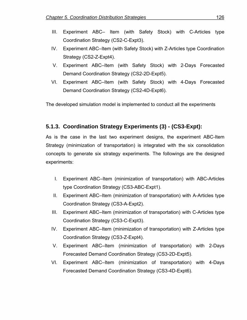
Chapter 5. Coordination Distribution Strategies 126
III. Experiment ABC– Item (with Safety Stock) with C-Articles type
Coordination Strategy (CS2-C-Expt3).
IV. Experiment ABC–Item (with Safety Stock) with Z-Articles type Coordination
Strategy (CS2-Z-Expt4).
V. Experiment ABC–Item (with Safety Stock) with 2-Days Forecasted
Demand Coordination Strategy (CS2-2D-Expt5).
VI. Experiment ABC–Item (with Safety Stock) with 4-Days Forecasted
Demand Coordination Strategy (CS2-4D-Expt6).
The developed simulation model is implemented to conduct all the experiments
5.1.3. Coordination Strategy Experiments (3) - (CS3-Expt):
As is the case in the last two experiment designs, the experiment ABC-Item
Strategy (minimization of transportation) is integrated with the six consolidation
concepts to generate six strategy experiments. The followings are the designed
experiments:
I. Experiment ABC–Item (minimization of transportation) with ABC-Articles
type Coordination Strategy (CS3-ABC-Expt1).
II. Experiment ABC–Item (minimization of transportation) with A-Articles type
Coordination Strategy (CS3-A-Expt2).
III. Experiment ABC–Item (minimization of transportation) with C-Articles type
Coordination Strategy (CS3-C-Expt3).
IV. Experiment ABC–Item (minimization of transportation) with Z-Articles type
Coordination Strategy (CS3-Z-Expt4).
V. Experiment ABC–Item (minimization of transportation) with 2-Days
Forecasted Demand Coordination Strategy (CS3-2D-Expt5).
VI. Experiment ABC–Item (minimization of transportation) with 4-Days
Forecasted Demand Coordination Strategy (CS3-4D-Expt6).

Chapter 5. Coordination Distribution Strategies 127
5.1.4. Coordination Strategy Experiments (4) - (CS4-Expt):
To study the effect of consolidation concepts on the allocation strategy only four
consolidation concepts are selected to coordinate with the base strategy
(Experiment C-Item Allocation Coordination Strategy). Four new coordination
strategies are constructed. These are:
I. Experiment C-Item Allocation with ABC-Articles type Coordination Strategy
(CS4-ABC-Expt1).
II. Experiment C-Item Allocation with C-Articles type Coordination Strategy
(CS4-C-Expt2).
III. Experiment C-Item Allocation with 2-Days Forecasted Demand
Coordination Strategy (CS4-2D-Expt3).
IV. Experiment C-Item Allocation with 4-Days Forecasted Demand
Coordination Strategy (CS4-4D-Expt4).
5.1.5. Coordination Strategy Experiments (5) - (CS5-Expt):
As is the case in the previous experiment design, four consolidation concepts are
selected and coordinated with the uncoordinated strategy (Experiment Z-Item
Allocation Strategy) to construct four coordination strategies. These strategies are:
I. Experiment Z-Item Allocation with ABC-Articles type Coordination Strategy
(CS5-ABC-Expt1).
II. Experiment Z-Item Allocation with Z-Articles type Coordination Strategy
(CS5-Z-Expt2).
III. Experiment Z-Item Allocation with 2-Days Forecasted Demand
Coordination Strategy (CS5-2D-Expt3).
IV. Experiment Z-Item Allocation with 4-Days Forecasted Demand
Coordination Strategy (CS5-4D-Expt4).

Chapter 5. Coordination Distribution Strategies 128
5.1.6. Coordination Strategy Experiments (6) - (CS6-Expt):
In this experiment design, all of the six consolidation concepts are selected and
integrated with the base strategy (Experiment CSL (80%) ABC Item Strategy) to
generate new six coordination strategies. The new coordination strategies will be
compared with the uncoordinated strategy (base). The descriptions of all the
experiments are:
I. Experiment CSL (80%) ABC Item with ABC-Articles type Coordination
Strategy (CS6-ABC-Expt1).
II. Experiment CSL (80%) ABC Item with A-Articles type Coordination
Strategy (CS6-A-Expt2).
III. Experiment CSL (80%) ABC Item with C-Articles type Coordination
Strategy (CS6-C-Expt3).
IV. Experiment CSL (80%) ABC Item with Z-Articles type Coordination
Strategy (CS6-Z-Expt4).
V. Experiment CSL (80%) ABC Item with 2-Days Forecasted Demand
Coordination Strategy (CS6-2D-Expt5).
VI. Experiment CSL (80%) ABC Item with 4-Days Forecasted Demand
Coordination Strategy (CS6-4D-Expt6).
5.1.7. Coordination Strategy Experiments (7) - (CS7-Expt):
This experiment design is the same as the above experiment design but the
difference is only in the selection of the uncoordinated strategy. The uncoordinated
strategy is the experiment CSL (90%) ABC Item Strategy (base). The six
generated strategy experiments are:
I. Experiment CSL (90%) ABC Item with ABC-Articles type Coordination
Strategy (CS7-ABC-Expt1).
II. Experiment CSL (90%) ABC Item with A-Articles type Coordination
Strategy (CS7-A-Expt2).

Chapter 5. Coordination Distribution Strategies 129
III. Experiment CSL (90%) ABC Item with C-Articles type Coordination
Strategy (CS7-C-Expt3).
IV. Experiment CSL (90%) ABC Item with Z-Articles type Coordination
Strategy (CS7-Z-Expt4).
V. Experiment CSL (90%) ABC Item with 2-Days Forecasted Demand
Coordination Strategy (CS7-2D-Expt5).
VI. Experiment CSL (90%) ABC Item with 4-Days Forecasted Demand
Coordination Strategy (CS7-4D-Expt6).
The general structure of the design of all the seven coordination strategies is
summarized in Table 5.1.
Table 5. 1 General Structure of Coordination Strategies Design
5.2. Experimental Simulation Results
Many results have been collected and analyzed after running the developed
simulation model for one year. The same measures of performance as used in the
last chapter are also calculated here. For comparing the results, the uncoordinated
strategies have been taken as the base experiments to be compared with the new
coordination strategies. The average order fill rate (AOFR) is selected as the first
and important measure of performance. The following section presents the results
and analysis of these results.
UCS- Expt 1 UCS- Expt 2 UCS- Expt 3 UCS- Expt 4 UCS- Expt 6 UCS- Expt 9 UCS- Expt 10 ABC A C Z 2D 4DCS1-Expt - - - - - -CS2-Expt - - - - - -CS3-Expt - - - - - -CS4-Expt - - - - - - -CS5-Expt - - - - - - - -CS6-Expt - - - - - -CS7-Expt - - - - - -
Integrated- Not Integrated
Expt-NameUncoordinated Strategy Expt. Consolidation Concept

Chapter 5. Coordination Distribution Strategies 130
5.2.1. Results of Coordination Strategy Experiments (1)
The simulation results of these experiments are summarized and the measures of
performance are calculated and ranked in ascending order based on the average
order fill rate (AOFR) as shown in Table 5.2 and Figure 5.1.
Table 5. 2 Measures of Performance of Each Coordination Strategy for Coordination Strategy Experiments (1)
Figure 5. 1 Measures of Performance of Each Strategy for Coordination Strategy Experiments (1)
Experiments TTC TIHC TLC AOLFR AOFRCS1-4D-Expt6 $8.039.851,27 $268.930,82 $8.308.782,09 98,87% 89,27%
CS1-ABC-Expt1 $8.687.533,81 $2.341.572,03 $11.029.105,84 98,74% 84,82%CS1-C-Expt3 $11.510.425,29 $5.717.147,31 $17.227.572,60 97,31% 68,04%CS1-A-Expt2 $10.639.802,17 $4.429.948,84 $15.069.751,01 97,55% 67,50%
CS1-2D-Expt5 $8.105.428,01 $274.111,20 $8.379.539,21 96,76% 66,13%CS1-Z-Expt4 $11.455.651,84 $5.574.419,35 $17.030.071,19 97,01% 65,92%UCS-Expt 1* $8.114.944,57 $276.000,10 $8.390.944,67 96,44% 61,06%
* Base Experiment
61,06%
65,92%
89,27%84,82%
68,04% 67,50% 66,13%
0,00E+00
2,00E+06
4,00E+06
6,00E+06
8,00E+06
1,00E+07
1,20E+07
1,40E+07
1,60E+07
1,80E+07
2,00E+07
CS1-4D-E
xpt6
CS1-ABC-E
xpt1
CS1-C-E
xpt3
CS1-A-E
xpt2
CS1-2D-E
xpt5
CS1-Z-E
xpt4
UCS-Exp
t 1*
Experiments
Cos
ts ($
)
0%
20%
40%
60%
80%
100%
120%
Fill
Rat
e
TTC TLC AOLFR AOFR

Chapter 5. Coordination Distribution Strategies 131
5.2.2. Results of Coordination Strategy Experiments (2)
The measures of performance of each strategy based on the ascending order of
average order fill rate (AOFR) are presented in Table 5.3 and Figure 5.2.
Table 5. 3 Measures of Performance of Each Coordination Strategy for Coordination Strategy Experiments (2)
Figure 5. 2 Measures of Performance of Each Strategy for Coordination Strategy Experiments (2)
Experiments TTC TIHC TLC AOLFR AOFRCS2-4D-Expt6 $8.132.842,11 $318.010,96 $8.450.853,07 99,69% 97,14%
CS2-ABC-Expt1 $8.945.934,57 $2.773.991,36 $11.719.925,93 99,53% 94,61%CS2-C-Expt3 $11.972.692,77 $6.399.221,14 $18.371.913,91 99,06% 88,12%CS2-Z-Expt4 $11.766.785,39 $6.048.990,65 $17.815.776,04 99,00% 88,05%CS2-A-Expt2 $11.003.937,31 $4.933.961,77 $15.937.899,08 99,09% 86,47%CS2-2D-Expt5 $8.146.000,17 $319.955,78 $8.465.955,95 98,82% 86,09%UCS-Expt 2* $8.149.488,60 $321.158,15 $8.470.646,75 98,68% 83,65%
* Base Experiment
83,65%
97,14% 94,61%88,12% 88,05% 86,47% 86,09%
0,00E+00
2,00E+06
4,00E+06
6,00E+06
8,00E+06
1,00E+07
1,20E+07
1,40E+07
1,60E+07
1,80E+07
2,00E+07
CS2-4D-E
xpt6
CS2-ABC-E
xpt1
CS2-C-E
xpt3
CS2-Z-E
xpt4
CS2-A-E
xpt2
CS2-2D-E
xpt5
UCS-Exp
t 2*
Experiments
Cos
ts ($
)
0%
20%
40%
60%
80%
100%
120%
Fill
Rat
e
TTC TLC AOLFR AOFR

Chapter 5. Coordination Distribution Strategies 132
5.2.3. Results of Coordination Strategy Experiments (3)
As in previous experiments, the measures of performance of each strategy are
given in Table 5.4 and Figure 5.3.
Table 5. 4 Measures of Performance of Each Coordination Strategy for Coordination Strategy Experiments (3)
Figure 5. 3 Measures of Performance of Each Strategy for Coordination Strategy Experiments (3)
Experiments TTC TIHC TLC AOLFR AOFRCS3-4D-Expt6 $8.103.591,95 $340.000,96 $8.443.592,91 99,50% 94,74%CS3-A-Expt2 $11.178.345,65 $5.185.475,66 $16.363.821,31 99,30% 89,54%
CS3-ABC-Expt1 $8.788.238,45 $2.578.447,63 $11.366.686,08 99,12% 89,16%CS3-Z-Expt4 $11.767.926,44 $6.067.614,39 $17.835.540,83 98,44% 80,67%
CS3-2D-Expt5 $8.121.995,18 $343.017,62 $8.465.012,80 98,30% 79,77%CS3-C-Expt3 $11.786.583,89 $6.155.959,19 $17.942.543,08 98,28% 78,40%UCS-Expt 3* $8.125.338,06 $344.206,49 $8.469.544,55 98,17% 77,19%
* Base Experiment
89,16%
78,40%79,77%
94,74% 89,54%
80,67%
77,19%
0,00E+00
2,00E+06
4,00E+06
6,00E+06
8,00E+06
1,00E+07
1,20E+07
1,40E+07
1,60E+07
1,80E+07
2,00E+07
CS3-4D-E
xpt6
CS3-A-E
xpt2
CS3-ABC-E
xpt1
CS3-Z-E
xpt4
CS3-2D-E
xpt5
CS3-C-E
xpt3
UCS-Exp
t 3*
Experiments
Cos
ts ($
)
0%
20%
40%
60%
80%
100%
120%
Fill
Rat
e
TTC TLC AOLFR AOFR

Chapter 5. Coordination Distribution Strategies 133
5.2.4. Results of Coordination Strategy Experiments (4)
The results of these experiments are shown in Table 5.5 and Figure 5.4.
Table 5. 5 Measures of Performance of Each Coordination Strategy for Coordination Strategy Experiments (4)
75,51%
62,99%
39,15%
80,82%
10,10%
0,00E+00
2,00E+06
4,00E+06
6,00E+06
8,00E+06
1,00E+07
1,20E+07
1,40E+07
1,60E+07
1,80E+07
2,00E+07
CS4-4D-E
xpt4
CS4-ABC-E
xpt1
CS4-C-E
xpt2
CS4-2D-E
xpt3
UCS-Exp
t 4*
Experiments
Cos
ts ($
)
0%
20%
40%
60%
80%
100%
120%
Fill
Rat
e
TTC TLC AOLFR AOFR
Figure 5. 4 Measures of Performance of Each Strategy for Coordination Strategy Experiments (4)
Experiments TTC TIHC TLC AOLFR AOFRCS4-4D-Expt4 $7.928.724,62 $180.621,99 $8.109.346,61 97,84% 80,82%
CS4-ABC-Expt1 $8.727.735,23 $2.348.033,66 $11.075.768,89 97,70% 75,51%CS4-C-Expt2 $11.519.417,05 $5.668.792,86 $17.188.209,91 96,69% 62,99%CS4-2D-Expt3 $8.007.420,01 $189.960,61 $8.197.380,62 92,50% 39,15%UCS-Expt 4* $8.109.584,95 $205.694,79 $8.315.279,74 86,49% 10,10%
* Base Experiment
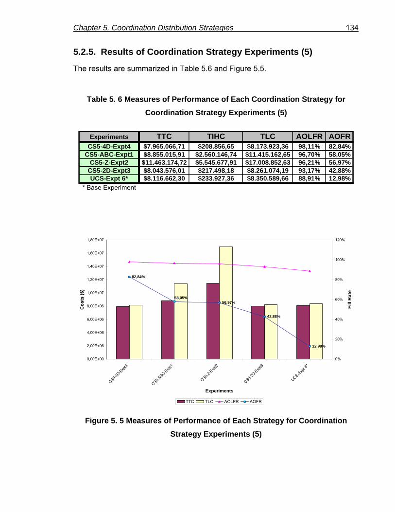
Chapter 5. Coordination Distribution Strategies 134
5.2.5. Results of Coordination Strategy Experiments (5)
The results are summarized in Table 5.6 and Figure 5.5.
Table 5. 6 Measures of Performance of Each Coordination Strategy for Coordination Strategy Experiments (5)
56,97%
42,88%
58,05%
82,84%
12,98%
0,00E+00
2,00E+06
4,00E+06
6,00E+06
8,00E+06
1,00E+07
1,20E+07
1,40E+07
1,60E+07
1,80E+07
CS5-4D-E
xpt4
CS5-ABC-E
xpt1
CS5-Z-E
xpt2
CS5-2D-E
xpt3
UCS-Exp
t 6*
Experiments
Cos
ts ($
)
0%
20%
40%
60%
80%
100%
120%
Fill
Rat
e
TTC TLC AOLFR AOFR
Figure 5. 5 Measures of Performance of Each Strategy for Coordination Strategy Experiments (5)
Experiments TTC TIHC TLC AOLFR AOFRCS5-4D-Expt4 $7.965.066,71 $208.856,65 $8.173.923,36 98,11% 82,84%
CS5-ABC-Expt1 $8.855.015,91 $2.560.146,74 $11.415.162,65 96,70% 58,05%CS5-Z-Expt2 $11.463.174,72 $5.545.677,91 $17.008.852,63 96,21% 56,97%
CS5-2D-Expt3 $8.043.576,01 $217.498,18 $8.261.074,19 93,17% 42,88%UCS-Expt 6* $8.116.662,30 $233.927,36 $8.350.589,66 88,91% 12,98%
* Base Experiment

Chapter 5. Coordination Distribution Strategies 135
5.2.6. Results of Coordination Strategy Experiments (6)
The measures of performance are estimated and presented in Table 5.7 and
Figure 5.6.
Table 5. 7 Measures of Performance of Each Coordination Strategy for Coordination Strategy Experiments (6)
Experiments TTC TIHC TLC AOLFR AOFRCS6-4D-Expt6 $8.113.603,89 $312.881,40 $8.426.485,29 99,52% 95,39%
CS6-ABC-Expt1 $8.863.932,25 $2.667.211,44 $11.531.143,69 99,35% 92,74%CS6-C-Expt3 $11.800.758,53 $6.157.632,97 $17.958.391,50 98,65% 83,03%CS6-A-Expt2 $10.894.912,99 $4.789.759,82 $15.684.672,81 98,82% 82,67%CS6-Z-Expt4 $11.642.805,24 $5.865.654,06 $17.508.459,30 98,49% 81,80%
CS6-2D-Expt5 $8.135.225,14 $315.905,35 $8.451.130,49 98,37% 81,02%UCS-Expt 9* $8.139.772,59 $317.015,50 $8.456.788,09 98,23% 78,45%
* Base Experiment
Figure 5. 6 Measures of Performance of Each Strategy for Coordination Strategy Experiments (6)
81,02%
92,74%95,39%83,03% 82,67% 81,80%
78,45%
0,00E+00
2,00E+06
4,00E+06
6,00E+06
8,00E+06
1,00E+07
1,20E+07
1,40E+07
1,60E+07
1,80E+07
2,00E+07
CS6-4D-E
xpt6
CS6-ABC-E
xpt1
CS6-C-E
xpt3
CS6-A-E
xpt2
CS6-Z-E
xpt4
CS6-2D-E
xpt5
UCS-Exp
t 9*
Experiments
Cos
ts ($
)
0%
20%
40%
60%
80%
100%
120%
Fill
Rat
e
TTC TLC AOLFR AOFR

Chapter 5. Coordination Distribution Strategies 136
5.2.7. Results of Coordination Strategy Experiments (7)
The measures of performance are calculated and presented in Table 5.8 and
Figure 5.7.
Table 5. 8 Measures of Performance of Each Coordination Strategy for Coordination Strategy Experiments (7)
Experiments TTC TIHC TLC AOLFR AOFRCS7-4D-Expt6 $8.128.735,31 $338.034,68 $8.466.769,99 99,69% 96,78%
CS7-ABC-Expt1 $9.011.188,75 $2.876.555,01 $11.887.743,76 99,52% 94,60%CS7-C-Expt3 $11.959.254,33 $6.387.193,00 $18.346.447,33 99,02% 87,52%CS7-A-Expt2 $10.996.591,27 $4.974.371,04 $15.970.962,31 99,17% 87,38%CS7-Z-Expt4 $11.739.426,40 $6.030.849,88 $17.770.276,28 98,92% 87,06%
CS7-2D-Expt5 $8.148.532,70 $340.068,95 $8.488.601,65 98,83% 86,12%UCS-Expt 10* $8.150.344,06 $340.914,26 $8.491.258,32 98,72% 84,08%
* Base Experiment
86,12% 84,08%87,06%87,38%87,52%
94,60%96,78%
0,00E+00
2,00E+06
4,00E+06
6,00E+06
8,00E+06
1,00E+07
1,20E+07
1,40E+07
1,60E+07
1,80E+07
2,00E+07
CS7-4D-E
xpt6
CS7-ABC-E
xpt1
CS7-C-E
xpt3
CS7-A-E
xpt2
CS7-Z-E
xpt4
CS7-2D-E
xpt5
UCS-Exp
t 10*
Experiments
Cos
ts ($
)
0%
20%
40%
60%
80%
100%
120%
Fill
Rat
e
TTC TLC AOLFR AOFR
Figure 5. 7 Measures of Performance of Each Strategy for Coordination Strategy Experiments (7)

Chapter 5. Coordination Distribution Strategies 137
5.3. Analysis of Simulation Results
In this section all the analysis and interpretation of the results (measures of
performance) are presented.
5.3.1. Logistics Costs and Fill Rate Analysis
From the investigations of the previous tables and figures, some findings are
notable:
• Coordination strategies perform better than the uncoordinated
strategies.
• In all seven experiments the 4-Days Forecasted Demand and the
ABC-Articles type consolidation concepts are the optimal strategies
for improving the uncoordinated strategies and system
performances, respectively, especially in terms of OFR.
The above findings can be proven by selecting CS6-Expt coordination experiment
design as an example. The improvement on the average of the order fill rate using
each consolidation concept is calculated as a percentage of the base experiment
(uncoordinated strategy) using equation (5.1) and shown in Figure 5.8.
Improvement of Average Order Fill Rate by each Coordination Strategy (%) =
%100xstrategyteduncoordinaofAOFR
strategyteduncoordinaofAOFRstrategyoncoordinatiofAOFR − (5.1)

Chapter 5. Coordination Distribution Strategies 138
18,22%
21,60%
5,84%5,38%
0,00%
3,28%4,27%
0%
5%
10%
15%
20%
25%
UCS-Exp
t 9*
CS6-2D-E
xpt5
CS6-Z-E
xpt4
CS6-A-E
xpt2
CS6-C-E
xpt3
CS6-ABC-E
xpt1
CS6-4D-E
xpt6
Experiments
Imp.
AO
FR (%
)
Figure 5. 8 Improvement of Order Fill Rate by Using Selected Consolidation
Concepts in Coordination Strategy Experiments (6)
Additionally, the percentage of increase in the total logistics costs resulting from
applying of the coordination strategies as compared with the uncoordinated
strategy (base) is calculated using equation (5.2) and shown in Figure 5.9.
Increase in Total Logistics Costs by Each Coordination Strategy (%) =
%100xstrategyteduncoordinaofTLC
strategyteduncoordinaofTLCstrategyoncoordinatiofTLC − (5.2)

Chapter 5. Coordination Distribution Strategies 139
0,00%
36,35%
85,47%
107,03%112,35%
-0,07%-0,36%
-20%
0%
20%
40%
60%
80%
100%
120%
CS6-4D-E
xpt6
CS6-2D-E
xpt5
UCS-Exp
t 9*
CS6-ABC-E
xpt1
CS6-A-E
xpt2
CS6-Z-E
xpt4
CS6-C-E
xpt3
Experiments
Incr
easi
ng T
LC (%
)
Figure 5. 9 Increase in Total Logistics Costs by Using Selected Consolidation
Concepts in Coordination Strategy Experiments (6)
The optimality of the 4-Days Forecasted Demand consolidation concept can be
justified by the fact that, this concept produces less inventory and transportation
due to the strength of the logic of the concept as explained in chapter 3. By this
concept, the truck will be highly utilized and a greater saving on transportation cost
is achievable. By this concept the average ending inventory is also reduced due to
the fact that the stock level of most items will be increased more than the reorder
point (s). This reduces the number of replenishments which in turn reduces the
total replenishment quantities, especially when the control parameters (s, S) of
uncoordinated strategies produce large replenishment quantities. Detailed
explanation has been made in the next chapter.
• The value of improving the service level (order fill rate) by applying
coordination strategies is more attractive when there is inappropriate
uncoordinated strategy. To show this fact, five general coordination

Chapter 5. Coordination Distribution Strategies 140
design strategies with the two optimal consolidation concepts (4-Days
Forecasted Demand and the ABC-Articles type) for each coordination
design strategy are selected. For more comparisons, the percentage of
improving average order fill rate and the percentage of increasing or
decreasing the total logistics costs by the two consolidation concepts for
each coordination strategy are calculated using equations (5.1), (5.2)
and (5.3) and shown in Figures 5.10, 5.11, 5.12, and 5.13.
Decrease in Total Logistics Costs by Each Coordination Strategy (%) =
%100xstrategyteduncoordinaofTLC
strategyoncoordinatiofTLCstrategyteduncoordinaofTLC − (5.3)
21,60%22,74%
16,13%
46,19%
15,11%
0%
5%
10%
15%
20%
25%
30%
35%
40%
45%
50%
CS1-4D-E
xpt6
CS2-4D-E
xpt6
CS3-4D-E
xpt6
CS6-4D-E
xpt6
CS7-4D-E
xpt6
Experiments
Imp.
AO
FR (%
)
Figure 5. 10 Improvement in Order Fill Rate by 4-Days Forecasted Demand
Concept for Each Coordination Strategy

Chapter 5. Coordination Distribution Strategies 141
0,29%
0,98%
0,23%0,31%
0,36%
0,00%
0,20%
0,40%
0,60%
0,80%
1,00%
1,20%
CS1-4D-E
xpt6
CS2-4D-E
xpt6
CS3-4D-E
xpt6
CS6-4D-E
xpt6
CS7-4D-E
xpt6
Experiments
Dec
reas
ing
TLC
(%)
Figure 5. 11 Decrease in Total Logistics Costs by 4-Days Forecasted Demand Concept for Each Coordination Strategy
18,22%
12,51%
38,90%
15,51%
13,10%
0%
5%
10%
15%
20%
25%
30%
35%
40%
45%
CS1-ABC-E
xpt1
CS2-ABC-E
xpt1
CS3-ABC-E
xpt1
CS6-ABC-E
xpt1
CS7-ABC-E
xpt1
Experiments
Imp.
AO
FR (%
)
Figure 5. 12 Improvement in Order Fill Rate by ABC-Articles type Concept for
Each Coordination Strategy

Chapter 5. Coordination Distribution Strategies 142
40,00%
36,35%34,21%38,36%
31,44%
0%
5%
10%
15%
20%
25%
30%
35%
40%
45%
CS1-ABC-E
xpt1
CS2-ABC-E
xpt1
CS3-ABC-E
xpt1
CS6-ABC-E
xpt1
CS7-ABC-E
xpt1
Experiments
Incr
easi
ng T
LC (%
)
Figure 5. 13 Increase in Total Logistics Costs by ABC-Articles type Concept for Each Coordination Strategy
• The optimal consolidation concept (4-Days Forecasted Demand)
improves the service levels (AOFR) on the average by 24% without
increasing the total logistic costs (Figure 5.10 and Figure 5.11).
• The second optimal coordination strategy (ABC-Articles type) improves
the service levels (Order Fill Rate) on the average by 20% and increases
the total logistic costs on the average by 36% (Figure 5.12 and Figure
5.13).
• The figures (5.10and 5.12) illustrate that the service level (Order Fill
Rate) of inappropriate distribution strategies is highly improved by using
an appropriate coordination strategy.
• In most of the experiments the A-Articles type consolidation concept
strategy performs better than the C-Articles type consolidation concept

Chapter 5. Coordination Distribution Strategies 143
for improving system performances in terms of total logistics costs. In
some cases, however, C-type articles consolidation concept gives a
slight improvement in the Average Order Fill Rate. To show this, the
coordination strategy experiments (1) - (CS1-Expt) are selected and the
results are show in Figure 5.14 and Figure 5.15. It can be explained by
the fact that the C-items represent the highest percentage of the total
items, as shown in Table 4.1 and Figure 4.5. This percentage affects the
availability of items and, therefore, the C-type articles (Items)
consolidation concept increases the availability of C-items at the
downstream locations which finally increases the efficiency of delivering
the completed orders (AOFR). The significant differences in measures of
performance by using these two consolidation concepts (A and C)
enhance the importance of using an appropriate items classification
approach, as will be seen in the next chapter.
0,00%
46,19%
7,95% 8,29%
11,42%10,54%
38,90%
0%
5%
10%
15%
20%
25%
30%
35%
40%
45%
50%
UCS-Exp
t 1*
CS1-Z-E
xpt4
CS1-2D-E
xpt5
CS1-A-E
xpt2
CS1-C-E
xpt3
CS1-ABC-E
xpt1
CS1-4D-E
xpt6
Experiments
Imp.
AO
FR (%
)
Figure 5. 14 Improvement in Order Fill Rate by Using Selected Consolidation
Concepts in Coordination Strategy Experiments (1)

Chapter 5. Coordination Distribution Strategies 144
31,44%
105,31%
0,00%-0,98% -0,14%
79,60%
102,96%
-20%
0%
20%
40%
60%
80%
100%
120%
CS1-4D-E
xpt6
CS1-2D-E
xpt5
UCS-Exp
t 1*
CS1-ABC-E
xpt1
CS1-A-E
xpt2
CS1-Z-E
xpt4
CS1-C-E
xpt3
Experiments
Incr
easi
ng T
LC (%
)
Figure 5. 15 Increase in the Total Logistics Costs by Using Selected Consolidation Concepts in Coordination Strategy Experiments (1)
- The interaction between the design of reorder points based on item type and
the item classification consolidation concept is remarkable. For example,
from the results, it was clear that in most of the coordination experiments the
ABC-Articles type consolidation concept performs better than the other item
classification consolidation concepts (A, C and Z) especially when the
design of reorder points of all the items types is the same (Tables 5.2, 5.3,
5.7 and 5.8). In the coordination strategy experiments (3) the A-Articles
(Items) type consolidation concept performs better than the ABC-Articles
type consolidation concept in terms of AOFR (Table 5.4). This can be
justified by the fact that, the design of the reorder point of A item type in
uncoordinated strategy (UCS-Expt 3) is different from the other items types.
The value of the s parameter for A-type items is the smallest (Table 4.14).
Therefore the A-Articles (Items) type consolidation concept can increase the

Chapter 5. Coordination Distribution Strategies 145
availability of A items which increases the efficiency of delivering the
completed orders (AOFR). This means that the reorder point of A item type
is inappropriate and should be redesigned. Also, for further explanation of
this interaction, consider as an example the coordination strategy
experiments (2) where the uncoordinated strategy (UCS- 2) gives more
values of the s parameter for A-type items (More safety stock), the A-
Articles (Items) type consolidation concept performs very badly compared to
other consolidation concepts ( Table 5.3). This means that the reorder point
(s) of A items type was designed perfectly by uncoordinated strategy and
there is no need to increase the availability of this item type. Furthermore,
the ABC-Articles type consolidation concept in the coordination strategy
experiments (2) performs better than in the other coordination strategy
experiments in terms of AOFR. This is interpreted by the good design of the
reorder points (s) of all items types (A, B and C) by the uncoordinated
strategy (UCS- 2).
- In most cases the TLC and AOLFR is correlated with AOFR.
Here, the problem of the large increase in the percentage of total logistics cost
is recognized, especially when the item (Article) classification consolidation
concept is used in coordination strategies. This is mainly due to the huge size
of shipment quantity (replenishment quantity) which was produced from the
logic of these consolidation concepts. The increase in the shipment size causes
an increase both in transportation and inventory costs. The problem is mainly
due to the complex structure of transportation cost rates in the considered real
life problem (Table 3.20). The potential saving in transportation cost by using a
full truck load under this cost structure is not really attractive. The relationship
between the pallet number and the discount in cost tariff is not linear, as shown
in Figures 5.16, 5.17, and 5.18. To explain that, the data from Table 3.20 is
illustrated in Figure 5.19 and is used to calculate the correlation coefficient
between the number of pallets and the transportation cost reduction for the

Chapter 5. Coordination Distribution Strategies 146
selected three regional distribution centers. The correlation coefficients are
shown in Table 5.9. The relationship between the number of pallets and the
truck utilization is also presented in Figure 5.20. In general, a uniform increase
in truck utilization for n total number of pallets may be expressed as U, 2U,
……………., (n-1)U .
Table 5. 9 Correlation Coefficient between Number of Pallets and Reduction in Transportation Cost
Figure 5. 16 Real Curve and Fitted Curve of Transportation Cost ($) Function in RDC9
DC Correlation Coefficient RDC9 0,741851974RDC13 0,773806665RDC19 0,857383295

Chapter 5. Coordination Distribution Strategies 147
Figure 5. 17 Real Curve and Fitted Curve of Transportation Cost ($) Function in RDC13
Figure 5. 18 Real Curve and Fitted Curve of Transportation Cost ($) Function in RDC19

Chapter 5. Coordination Distribution Strategies 148
0%
10%
20%
30%
40%
50%
60%
70%
80%
90%
100%
1 2 3 4 5 6 7 8 9 10 11 12 13 14 15 16 17 18 19 20 21 22 23 24 25 26 27 28 29 30 31 32 33 34 35 36 37 38
Number of Pallets
Red
uctio
n in
Cos
t (%
)
Distribution Center Nr. RDC9 Distribution Center Nr. RDC13 Distribution Center Nr. RDC19 Figure 5. 19 Reduction in Transportation Cost
0%
10%
20%
30%
40%
50%
60%
70%
80%
90%
100%
110%
0 1 2 3 4 5 6 7 8 9 10 11 12 13 14 15 16 17 18 19 20 21 22 23 24 25 26 27 28 29 30 31 32 33 34 35 36 37 38
Number of Pallets
Util
izat
ion(
%)
Figure 5. 20 Relationship between the Number of Pallets and the Truck
Utilization

Chapter 5. Coordination Distribution Strategies 149
As mentioned above, one of the disadvantages of using coordination strategies is
the increase in the average inventory level. When items are coordinated, some of
them will be replenished earlier than if they were treated independently. This
problem is named as residual stock [SPP98] and will be discussed in more details
in the next section. Increasing the average inventory level is considered for
redesigning the reorder point as safety stock. Then the uncoordinated strategy with
consolidation concept (coordination strategy) is compared with the uncoordinated
strategy with increasing reorder point (More Safety Stock). The idea is to use the
residual stock as safety stock built into the reorder point. Based on this idea the
equation for increasing the level of inventory from the coordination strategy,
considered as safety stock instead of redesigning of the reorder point by adding
safety stock, is created. The following are the experiments selected to carry out a
comparison study for this purpose:
Experiment ABC– Item Strategy (without Safety Stock) - (UCS- Expt
1)
Experiment ABC-Item Strategy (with Safety Stock) - (UCS- Expt 2)
Experiment ABC– Item (without Safety Stock) with ABC-Articles
(Items) type Coordination Strategy (CS1-ABC-Expt1)
Experiment ABC– Item (without Safety Stock) 4-Days Forecasted
Demand Coordination Strategy (CS1-4D-Expt6)
The first strategy is designed without considering of the safety stock, the
second strategy is designed with more consideration of the safety (Table 4.14),
and the third and fourth strategies are coordination strategies of the first
strategy (Table 5.1).
The results of all the strategies are compared and summarized in Table 5.10
and Table 5.11.

Chapter 5. Coordination Distribution Strategies 150
Table 5. 10 Improving Order Fill Rate of the Four Selected Experiments
Table 5. 11 Increasing Total Logistics Costs of the Four Selected Experiments
The above tables show that, the coordination strategies can improve the service
level better than redesigning the reorder point with more safety stock does. So it is
recommended that to improve service level, coordination strategies should be used
rather than increasing the safety stock policy. For example, the (CS1-4D-Expt6)
coordination strategy improves the Order Fill Rate of (UCS- Expt 1) uncoordinated
strategy by 46% without increasing the total logistic costs and in the same time the
(UCS- Expt 2) uncoordinated strategy (More safety stock) improves the Order Fill
Rate by 36% with increasing the total logistic costs. Therefore, instead of thinking
of increasing the safety stock for improving the service level, more attention should
be paid to applying coordination strategies.
Experiments Increasing Total Logistics Cost (%)CS1-4D-Expt6 -0,98%
CS1-ABC-Expt1 31,44%UCS-Expt 2 0,95%UCS-Expt 1* 0,00%
* Base Experiment
Experiments Improving Average Order Fill Rate (%)CS1-4D-Expt6 46,19%
CS1-ABC-Expt1 38,90%UCS-Expt 2 36,98%UCS-Expt 1* 0,00%
* Base Experiment
Chapter 5. Coordination Distribution Strategies 151
5.3.2. Residual Stock Analysis
In this section the problem of increasing the stock level in distribution centers
caused by consolidation concepts in coordination strategies is discussed. The
increasing results when an item is reordered while it is still above its reorder point.
This is because some other items in the distribution center will trigger the
replenishment. The excess stock above the reorder point is known as residual
stock [SPP98]. The residual stock must be taken into account because it adds
safety stock above and beyond the usual safety stock included in the reorder point.
All the used consolidation concepts cause this problem. Detailed investigations and
analysis have been done and the main points are explored. Statistical analysis
tests are performed to fit the residual stock distribution from different consolidation
concepts. Therefore, many items from different distribution centers are selected
and fitted by using the supported tool "Input Analyzer" of Arena 5.0 Software
(Rockwell Software, [KSS02]). The results of the experiment coordination strategy
experiments (3) and uncoordinated strategy “experiment ABC-Item strategy
(minimize of transportation)” are taken as a base experiment for performing this
analysis. Two distribution centers are also selected: RDC17 and RDC19. As
discussed in the literature, Miltenburg and Silver [MS84] have found that in a
periodic review system a normal distribution provides a reasonable fit to the
distribution of residual stock. In this thesis, the continuous review with (s, S) control
policy is used, and the best fit for residual stock for most consolidation concepts is
found to be the normal distribution. For example, for an A-item using an ABC-
Articles type Consolidation Concept, the best fit to the distribution of residual stock
is normal distribution (Square Error: 0.014247) and the same item using (4-Days
Forecasted Demand) consolidation concept, the best fit to the distribution of
residual stock is exponential distribution (Square Error: 0.007835). Such
distributions must be taken into account when establishing the reorder points (as
safety stock).
The summarized results of the analyzed residual stock for both distribution centers
are shown in Figure 5.21 and Figure 5.22.

Chapter 5. Coordination Distribution Strategies 152
-0,80%0,00%
0,21%2,11%
3,74%
9,84%
35,54%
-5%
0%
5%
10%
15%
20%
25%
30%
35%
40%
CS3-2D
-Exp
t5
UCS-Exp
t 3*
CS3-C-E
xpt3
CS3-ABC-E
xpt1
CS3-4D
-Exp
t6
CS3-Z-
Expt4
CS3-A-E
xpt2
Experiments
Res
idua
l Sto
ck
* Base Experiment
Figure 5. 21 Percentage of Increase in the Average Residual Stock by Each Consolidation Concept in RDC17 [A-Item]
1936,91%
39,79%29,00%8,20%4,69%
-1,17% 0,00%
-500%
0%
500%
1000%
1500%
2000%
2500%
CS3-C-E
xpt3
UCS-Exp
t 3*
CS3-2D-E
xpt5
CS3-4D-E
xpt6
CS3-ABC-E
xpt1
CS3-Z-E
xpt4
CS3-A-E
xpt2
Experiments
Res
idua
l Sto
ck
* Base Experiment
Figure 5. 22 Percentage of Increase in the Average Residual Stock by Each Consolidation Concept in RDC19 [A-Item]

Chapter 5. Coordination Distribution Strategies 153
The Residual stock chart of 4-Days Forecasted Demand consolidation concept for
RDC19 is shown in Figure 5.23. The peak point of the residual is seen in the month
of December because of the huge demand rate in this month. This proves that this
consolidation concept can handle the seasonality of demand with perfect balance
of residual stock.
0
500
1000
1500
2000
2500
11-J
un
20-J
un
28-J
un
9-Ju
l
20-J
ul
1-A
ug
13-A
ug
22-A
ug
31-A
ug
10-S
ep
18-S
ep
27-S
ep
9-O
ct
25-O
ct
6-N
ov
15-N
ov
23-N
ov
5-D
ec
17-D
ec
27-D
ec
10-J
an
21-J
an
29-J
an
12-F
eb
22-F
eb
8-M
ar
19-M
ar
27-M
ar
5-Ap
r
16-A
pr
26-A
pr
13-M
ay
27-M
ay
Date
Stoc
k le
vel (
Bag
s)
Residual Stock Reoder Point
Figure 5. 23 Residual Stock and Reorder Point of A-Item Using 4-Days Forecasted Demand Consolidation Concept in RDC19
To control the residual stock, appropriate group replenishment should be selected.
This depends mainly on the number of items selected for consolidation, the
quantity of each item, and the average usage or demand rate. To show that, one
fast moving high demand variability item (ZA- Item) in the above two distribution
centers is selected. The residual stock of this item caused by two consolidation
concepts (Z-Articles and A- Articles) is calculated and shown in Figure 5.24 and
Figure 5.25, respectively.

Chapter 5. Coordination Distribution Strategies 154
In RDC19, the average residual stock of this item by using Z-Articles consolidation
concept is less than that when using A-Articles consolidation concept is used. It is
clear from due to the percentage of each item classification in this distribution. The
A-Item percentage is 18% and Z-Item is 50%. This means that the number of
consolidation items in Z-Articles consolidation concept is more than the number of
consolidation items in the A-Articles consolidation concept and the consolidated
quantity size of each item in Z-Articles consolidation concept is lower than the
consolidated quantity size of each item in the A-Articles consolidation concept
(Figure 5.24 and 5.25).
0
2
4
6
8
10
12
14
16
18
11-J
un
19-J
un
27-J
un
5-Ju
l
17-J
ul
25-J
ul
2-Au
g
10-A
ug
20-A
ug
28-A
ug
10-S
ep
19-S
ep
27-S
ep
9-O
ct
19-O
ct
29-O
ct
8-N
ov
16-N
ov
26-N
ov
6-D
ec
14-D
ec
2-Ja
n
10-J
an
21-J
an
29-J
an
6-Fe
b
21-F
eb
7-M
ar
15-M
ar
28-M
ar
5-A
pr
16-A
pr
26-A
pr
7-M
ay
22-M
ay
Date
Res
idua
l Sto
ck (
Palle
t)
Residual Stock(Pallet) Reoder Point(Pallet)
Figure 5. 24 Residual Stock of ZA Item Using (Z-Articles) Consolidation Concept in RDC19

Chapter 5. Coordination Distribution Strategies 155
0
10
20
30
40
50
60
70
80
90
100
110
5-Ju
n
20-J
un
3-Ju
l
16-J
ul
27-J
ul
9-A
ug
22-A
ug
4-S
ep
17-S
ep
28-S
ep
12-O
ct
26-O
ct
8-N
ov
21-N
ov
4-D
ec
17-D
ec
2-Ja
n
16-J
an
29-J
an
13-F
eb
28-F
eb
15-M
ar
28-M
ar
10-A
pr
25-A
pr
10-M
ay
24-M
ay
Date
Res
idua
l Sto
ck (
Palle
t)
Residual Stock(Pallet) Reoder Point(Pallet) Figure 5. 25 Residual Stock of ZA Item Using (A-Articles) Consolidation
Concept in RDC19
To explain the effect of consumption rate of each item on the residual stock, the
average residual stock of the same item (ZA item) in the two distribution centers is
compared and presented in the Figure 5.26. From this figure, the residual stock of
this item caused by consolidation concepts at RDC17 is less than that at RDC19.
This is due to the fact that the average demand rate of the item in RDC17 is
greater than that in RDC19 (Avg. Demand = 3 pallets & Avg. Demand = 1.5 pallets,
respectively). As mentioned in Chapter 3, the minimum quantity size of
consolidation of each item is equal to one pallet. Therefore, the consolidated load
in RDC17 is approximately 33% of the average demand rate whereas in RDC19 it
is approximately 67% of the average demand rate.

Chapter 5. Coordination Distribution Strategies 156
-5%
0%
5%
10%
15%
20%
25%
30%
35%
40%
45%
UCS-Exp
t 3*
CS3-2D-E
xpt5
CS3-4D-E
xpt6
CS3-C-E
xpt3
CS3-ABC-E
xpt1
CS3-Z-E
xpt4
Increased Average Residual Stock (%)_RDC19 Increased Average Residual Stock (%)_RDC17* Base Experiment Figure 5. 26 Comparison of Increasing Average Residual Stock (%) of ZA-
Item in Two Distribution Centers (RDC17 & RDC19)
One of the complex problems for controlling of the residual stock is the selection of
the proper quantity of consolidation groups. The studied model (real Model); it is
much more complex because the items are replenished from different suppliers.
So, it is not easy to control the consolidation shipment size. To explain this
problem, the percentage of supplying or replenishing A-Items from the three
suppliers (Warehouses) to each distribution center is calculated and the average
percentage of all distribution centers is estimated and presented in Figure 5.27.

Chapter 5. Coordination Distribution Strategies 157
15,42%
46,73%
37,85%
Warehouse(1) Warehouse(2) Warehouse(3)
Figure 5. 27 Average Percentage of A-Item from Suppliers (Warehouses) to Distribution Centers
When more items are consolidated with a proper consolidation quantity size, the
effect of residual stock will be reduced. This is due to the increase in the interval
period time between replenishments of many items. Increasing the interval period
between replenishments can reduce the number of replenishments, which finally
reduces the average ending inventory levels.
5.3.3. Truck Utilization Analysis:
As mentioned in Chapter 3, the item classification consolidation concepts can
guarantee that the replenishment quantities will generate a full truckload. From the
results, all the Item classification consolidation concepts produce 100% utilization
of truck. To show the effect of the coordination strategies on the utilization of truck,
as it is done in the previous chapter, the truck utilization between the upstream
locations and RDC15 for each coordination strategy with the 4-Days Forecasted
Demand consolidation concept is presented in Figure 5.28.

Chapter 5. Coordination Distribution Strategies 158
0%
10%
20%
30%
40%
50%
60%
70%
80%
90%
100%
CS1-4D-E
xpt6
CS2-4D-E
xpt6
CS3-4D-E
xpt6
CS4-4D-E
xpt4
CS5-4D-E
xpt4
CS6-4D-E
xpt6
CS7-4D-E
xpt6
Experiments
Truc
k U
tiliz
atio
n (%
)
Warehouse 1 Warehouse 2 Warehouse 3 Figure 5. 28 Truck Utilization between Upstream Locations and RDC15
From Figure 5.28, it is clear that the truck utilization is improved by using the
coordination strategies, which is 63% on the average. This figure is about 6%
higher than that for the uncoordinated strategies (Figure 4.24 and 5.28).

Chapter 5. Coordination Distribution Strategies 159
Conclusion:
Regarding the analysis and investigation of the results, the following
conclusions can be made:
• Classifications of items are very important for uncoordinated and
coordination strategies. Therefore, developing new classifications for
items that are considered more appropriate classification criteria
should be constructed.
• N-Days forecasted demand concepts are better than Item
classification consolidation concepts for designing effective
coordination strategies.
• Interaction between the reorder point design and the consolidation
concepts is remarkable. So more consideration of this interaction is
powerful for designing good coordination strategies.
• Coordination strategies which use Item classification consolidation
concepts raise the ending inventory very highly. While the
Coordination strategies which use N-Days forecasted demand
concepts reduce the ending inventory.
• Truck Utilization is yet not highly utilized by using the N-Days
forecasted demand concepts.
Chapter 6. Developing New ABC Classification 160
6. Optimization of Coordination Strategies: Developing New ABC Classification
In this chapter, the distribution coordination strategies have been optimized based
on the conclusions of the previous chapters. These conclusions are mainly
regarding the improvement of item classification approaches which could be used
in constructing an appropriate consolidation concept. Finally the appropriate
consolidation concept can improve the measures of performance of the distribution
coordination strategies. Therefore, in this chapter a new item classification
approach is presented.
6.1. New ABC Classification Model:
As a conclusion from last chapters, the right selection of item classification (More
frequent Items) is the key for getting the optimal coordination strategy. Therefore, a
new ABC Classification has been developed to optimize system performance. The
idea behind constructing this classification is to consolidate more ordered or
frequent items rather than items with high consumption rate. The consolidation of
more ordered items produces fewer replenishments that can finally reduce the
inventory and transportation cost. The New ABC classification will be integrated
with the Item classification consolidation concept to develop a new consolidation
concept that could improve the effectiveness of the old item consolidation concept.
The improvement in the systems performance by using this classification in item
consolidation concept has been proved and presented in this chapter.
As mentioned above, the items are classified based on the number of orders for
each item (order lines):
• A-Class: This class represents about 24 to 50% of the items carried in
inventory and 75% of the total number of order lines.
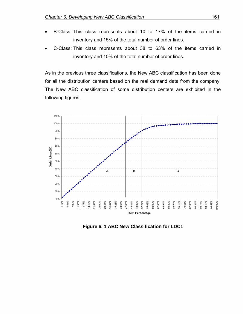
Chapter 6. Developing New ABC Classification 161
• B-Class: This class represents about 10 to 17% of the items carried in
inventory and 15% of the total number of order lines.
• C-Class: This class represents about 38 to 63% of the items carried in
inventory and 10% of the total number of order lines.
As in the previous three classifications, the New ABC classification has been done
for all the distribution centers based on the real demand data from the company.
The New ABC classification of some distribution centers are exhibited in the
following figures.
0%
10%
20%
30%
40%
50%
60%
70%
80%
90%
100%
110%
1,14
%
4,55
%
7,95
%
11,3
6%
14,7
7%
18,1
8%
21,5
9%
25,0
0%
28,4
1%
31,8
2%
35,2
3%
38,6
4%
42,0
5%
45,4
5%
48,8
6%
52,2
7%
55,6
8%
59,0
9%
62,5
0%
65,9
1%
69,3
2%
72,7
3%
76,1
4%
79,5
5%
82,9
5%
86,3
6%
89,7
7%
93,1
8%
96,5
9%
100,
00%
Item Percentage
Ord
er L
ines
(%)
A B C
Figure 6. 1 ABC New Classification for LDC1

Chapter 6. Developing New ABC Classification 162
0%
10%
20%
30%
40%
50%
60%
70%
80%
90%
100%
110%
1,09
%
4,35
%
7,61
%
10,8
7%
14,1
3%
17,3
9%
20,6
5%
23,9
1%
27,1
7%
30,4
3%
33,7
0%
36,9
6%
40,2
2%
43,4
8%
46,7
4%
50,0
0%
53,2
6%
56,5
2%
59,7
8%
63,0
4%
66,3
0%
69,5
7%
72,8
3%
76,0
9%
79,3
5%
82,6
1%
85,8
7%
89,1
3%
92,3
9%
95,6
5%
98,9
1%
Item Percentage
Ord
er L
ines
(%)
A B C
Figure 6. 2 ABC New Classification for LDC5
0%
10%
20%
30%
40%
50%
60%
70%
80%
90%
100%
110%
0,89
%
3,57
%
6,25
%
8,93
%
11,6
1%
14,2
9%
16,9
6%
19,6
4%
22,3
2%
25,0
0%
27,6
8%
30,3
6%
33,0
4%
35,7
1%
38,3
9%
41,0
7%
43,7
5%
46,4
3%
49,1
1%
51,7
9%
54,4
6%
57,1
4%
59,8
2%
62,5
0%
65,1
8%
67,8
6%
70,5
4%
73,2
1%
75,8
9%
78,5
7%
81,2
5%
83,9
3%
86,6
1%
89,2
9%
91,9
6%
94,6
4%
97,3
2%
100,
00%
Item Percentage
Ord
er L
ines
(%)
A B C
Figure 6. 3 ABC New Classification for RDC15

Chapter 6. Developing New ABC Classification 163
0%
10%
20%
30%
40%
50%
60%
70%
80%
90%
100%
110%
0,92
%
3,67
%
6,42
%
9,17
%
11,9
3%
14,6
8%
17,4
3%
20,1
8%
22,9
4%
25,6
9%
28,4
4%
31,1
9%
33,9
4%
36,7
0%
39,4
5%
42,2
0%
44,9
5%
47,7
1%
50,4
6%
53,2
1%
55,9
6%
58,7
2%
61,4
7%
64,2
2%
66,9
7%
69,7
2%
72,4
8%
75,2
3%
77,9
8%
80,7
3%
83,4
9%
86,2
4%
88,9
9%
91,7
4%
94,5
0%
97,2
5%
100,
00%
Item Percentage
Ord
er L
ines
(%)
A B C
Figure 6. 4 ABC New Classification for RDC19
The percentage of items in each class for each distribution center is exhibited in
Table 6.1.
Table 6. 1 Percentage of Items in each Class for each Distribution Center
(New ABC Classification)
D C A B C T o ta lR D C 1 30 ,19% 14 ,15% 55 ,66% 100 ,00%R D C 2 33 ,33% 15 ,74% 50 ,93% 100 ,00%R D C 3 31 ,86% 13 ,27% 54 ,87% 100 ,00%R D C 4 35 ,58% 14 ,42% 50 ,00% 100 ,00%R D C 5 34 ,55% 12 ,73% 52 ,73% 100 ,00%R D C 6 24 ,63% 12 ,69% 62 ,69% 100 ,00%R D C 7 29 ,82% 14 ,04% 56 ,14% 100 ,00%R D C 8 30 ,28% 11 ,93% 57 ,80% 100 ,00%R D C 9 28 ,70% 10 ,19% 61 ,11% 100 ,00%
R D C 10 30 ,91% 13 ,64% 55 ,45% 100 ,00%R D C 11 27 ,52% 13 ,76% 58 ,72% 100 ,00%R D C 12 32 ,71% 13 ,08% 54 ,21% 100 ,00%R D C 13 32 ,74% 13 ,27% 53 ,98% 100 ,00%R D C 14 32 ,17% 13 ,04% 54 ,78% 100 ,00%R D C 15 28 ,57% 13 ,39% 58 ,04% 100 ,00%R D C 16 27 ,88% 15 ,38% 56 ,73% 100 ,00%R D C 17 28 ,80% 11 ,20% 60 ,00% 100 ,00%R D C 18 31 ,78% 13 ,08% 55 ,14% 100 ,00%R D C 19 30 ,28% 16 ,51% 53 ,21% 100 ,00%L D C 1 40 ,91% 10 ,23% 48 ,86% 100 ,00%L D C 2 40 ,70% 11 ,63% 47 ,67% 100 ,00%L D C 3 39 ,02% 13 ,41% 47 ,56% 100 ,00%L D C 4 49 ,38% 12 ,35% 38 ,27% 100 ,00%L D C 5 43 ,48% 11 ,96% 44 ,57% 100 ,00%

Chapter 6. Developing New ABC Classification 164
To show the difference between the old ABC and the New ABC classifications, the
percentage of items in each class of the two classifications for all the distribution
centers are illustrated in the following Figures:
0%
5%
10%
15%
20%
25%
30%
35%
40%
45%
50%
55%
RDC1RDC2
RDC3RDC4
RDC5RDC6
RDC7RDC8
RDC9
RDC10
RDC11
RDC12
RDC13
RDC14
RDC15
RDC16
RDC17
RDC18
RDC19LD
C1LD
C2LD
C3LD
C4LD
C5
Distribution Center
Perc
enta
ge o
f Ite
ms
New A-Class Old A-Class Figure 6. 5 Percentage of Items in A Class for each Distribution Center in
Two Classifications

Chapter 6. Developing New ABC Classification 165
0%
5%
10%
15%
20%
25%
RDC1RDC2
RDC3RDC4
RDC5RDC6
RDC7RDC8
RDC9
RDC10
RDC11
RDC12
RDC13
RDC14
RDC15
RDC16
RDC17
RDC18
RDC19LD
C1LD
C2LD
C3LD
C4LD
C5
Distribution Center
Perc
enta
ge o
f Ite
ms
New B-Class Old B-Class Figure 6. 6 Percentage of Items in B Class for each Distribution Center in the
two Classifications
0%
10%
20%
30%
40%
50%
60%
70%
80%
RDC1RDC2
RDC3RDC4
RDC5RDC6
RDC7RDC8
RDC9
RDC10
RDC11
RDC12
RDC13
RDC14
RDC15
RDC16
RDC17
RDC18
RDC19LD
C1LD
C2LD
C3LD
C4LD
C5
Distribution Center
Perc
enta
ge o
f Ite
ms
New C-Class Old C-Class Figure 6. 7 Percentage of Items in C Class for each Distribution Center in the
two Classifications

Chapter 6. Developing New ABC Classification 166
The average percentage of items in each class of the two classifications for all the
distribution centers is shown in Figure 6.8.
19,41% 18,03%
62,55%
33,16%
13,13%
53,71%
0%
10%
20%
30%
40%
50%
60%
70%
A B C
ABC Classes
Perc
enta
ge o
f Ite
ms
Average (Old) Average (New) Figure 6. 8 Average Percentages of Items in each Class for the two
Classifications
6.2. Experiments Designs
In these experiment designs, the New ABC classification has been used to design
the control parameters (s, S) in uncoordinated strategies and Item classification
consolidation concept in coordination strategies.
In this section, three general experiments are considered and conducted by
implementing the developed simulation model as is the case in the previous
chapters. All the assumptions and considerations used in the last two chapters are
used in these experiments, too.
- UCS-N-Expt: Uncoordinated Strategy with new ABC classification experiment.

Chapter 6. Developing New ABC Classification 167
- CS-N-Expt: Coordination Strategy with new ABC classification experiment
6.2.1. Experiment New-ABC-Item Uncoordinated Strategy - (UCS-N-Expt):
Based on the New ABC Classification, the reorder point and the maximum
inventory level for each item are designed. To estimate these two parameters the
general equation (4.4) is used. Table 6.2 shows the number of days given for each
parameter.
Table 6. 2 Reorder Point and Maximum Inventory Level for Each Item Class
As can bee seen in the above table and Table 4.5, the logic of designing the
control parameters (s, S) in this strategy is same as in the uncoordinated strategy
(Experiment ABC-Item Strategy, UCS- Expt 3) in Chapter 4. The reason for that is
to enhance the importance of item classifications on the effectiveness of the
distribution strategies.
6.2.2. Experiments New-ABC-Item Coordination Strategy (1) - (CS1-N-Expt):
The main goal of this experiment design is to prove that the coordination strategies
are still better than uncoordinated strategies, even with a new ABC classification
and also to show the effect of using the new ABC classification in the Item
classification consolidation concept on the performance of the coordination
strategies.
New ABC Classification s (Days) S (Days)A 4 10B 6 10C 10 15
Chapter 6. Developing New ABC Classification 168
The New ABC Classification has been used to develop the following three new
Item consolidation concepts. These three concepts are as follows:
1. Full Truck Load with New-ABC-Articles type.
2. Full Truck Load with New-A-Articles type.
3. Full Truck Load with New-C-Articles type.
In this experiments design, the Experiment New-ABC-Item Uncoordinated Strategy
(UCS-N-Expt) is integrated with all the above consolidation concepts and also with
two of the N-Days forecasted demand consolidation concepts to generate five new
experiments. The name of each experiment strategy is described as follows:
1. Experiment New-ABC-Item Uncoordinated Strategy with New-ABC-Articles
(CS1-N-ABC-Expt1)
2. Experiment New-ABC-Item Uncoordinated Strategy with New-A-Articles (CS1-
N-A-Expt2)
3. Experiment New-ABC-Item Uncoordinated Strategy with New-C-Articles (CS1-
N-C-Expt3)
4. Experiment New-ABC-Item Uncoordinated Strategy with 2-Days Forecasted
Demand (CS1-N-2D-Expt4).
5. Experiment New-ABC-Item Uncoordinated Strategy with 4-Days Forecasted
Demand (CS1-N-4D-Expt5).
As mentioned before, all the experiments are conducted by using the developed
simulation model.

Chapter 6. Developing New ABC Classification 169
6.2.3. Experiments New-ABC-Item Coordination Strategy (2) - (CS2-N-Expt):
To prove the importance of item classification in consolidation and optimization of
system performance, new experiments are designed and compared with old
experiments to show how this new classification can optimize system performance.
As is the case in the previous experiment design, to design coordination strategies
of these new experiments, the uncoordinated strategy (UCS- Expt 1) of Chapter 4
is integrated with the three new consolidation concepts developed in this chapter to
generate three new experiments, which are:
1. UCS- Expt 1With New-ABC-Articles (CS2-N-ABC-Expt1).
2. UCS- Expt 1With New-A-Articles (CS2-N-A-Expt2).
3. UCS- Expt 1With New-C-Articles (CS2-N-C-Expt3).
The general structure of designing the two coordination strategies by using the new
ABC classification is summarized in Table 6.3.
Table 6. 3 General Structure of Coordination Strategies Design Using the New ABC Classification
UCS-N-Expt UCS- Expt 1 New-ABC New-A New-C 2D 4DCS1-N-Expt -CS2-N-Expt - - -
Integrated- Not Integrated
Expt-NameUncoordinated Strategy Expt. Consolidation Concept
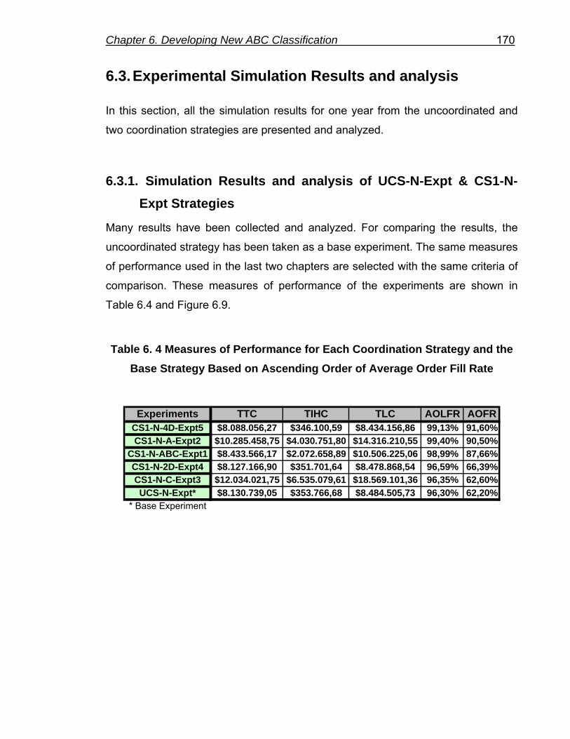
Chapter 6. Developing New ABC Classification 170
6.3. Experimental Simulation Results and analysis
In this section, all the simulation results for one year from the uncoordinated and
two coordination strategies are presented and analyzed.
6.3.1. Simulation Results and analysis of UCS-N-Expt & CS1-N-Expt Strategies
Many results have been collected and analyzed. For comparing the results, the
uncoordinated strategy has been taken as a base experiment. The same measures
of performance used in the last two chapters are selected with the same criteria of
comparison. These measures of performance of the experiments are shown in
Table 6.4 and Figure 6.9.
Table 6. 4 Measures of Performance for Each Coordination Strategy and the Base Strategy Based on Ascending Order of Average Order Fill Rate
Experiments TTC TIHC TLC AOLFR AOFRCS1-N-4D-Expt5 $8.088.056,27 $346.100,59 $8.434.156,86 99,13% 91,60%CS1-N-A-Expt2 $10.285.458,75 $4.030.751,80 $14.316.210,55 99,40% 90,50%
CS1-N-ABC-Expt1 $8.433.566,17 $2.072.658,89 $10.506.225,06 98,99% 87,66%CS1-N-2D-Expt4 $8.127.166,90 $351.701,64 $8.478.868,54 96,59% 66,39%CS1-N-C-Expt3 $12.034.021,75 $6.535.079,61 $18.569.101,36 96,35% 62,60%UCS-N-Expt* $8.130.739,05 $353.766,68 $8.484.505,73 96,30% 62,20%
* Base Experiment

Chapter 6. Developing New ABC Classification 171
91,60% 90,50%87,66%
66,39%62,60% 62,20%
0,00E+00
2,00E+06
4,00E+06
6,00E+06
8,00E+06
1,00E+07
1,20E+07
1,40E+07
1,60E+07
1,80E+07
2,00E+07
CS1-N-4D
-Exp
t5
CS1-N-A
-Exp
t2
CS1-N-A
BC-Exp
t1
CS1-N-2D
-Exp
t4
CS1-N-C
-Exp
t3
UCS-N-E
xpt*
Experiments
Cos
ts($
)
0%
20%
40%
60%
80%
100%
120%
Fill
Rat
e
TTC TLC AOLFR AOFR
Figure 6. 9 Measures of Performance for Each Strategy Based on Ascending Order of Average Order Fill Rate
The percentage of improved average order fill rate and increased total logistics
costs are calculated using the two equations (5.1) and (5.2) and are presented in
Figure 6.10 and Figure 6.11, respectively.

Chapter 6. Developing New ABC Classification 172
0,00% 0,65%
6,73%
47,27%
40,92%
45,49%
0%
5%
10%
15%
20%
25%
30%
35%
40%
45%
50%
UCS-N-E
xpt*
CS1-N-C
-Exp
t3
CS1-N-2D
-Exp
t4
CS1-N-A
BC-Exp
t1
CS1-N-A
-Exp
t2
CS1-N-4D
-Exp
t5
Experiments
Imp.
AO
FR
Figure 6. 10 Percentage of Improved Order Fill Rate by each Coordination Strategy
0,00%
68,73%
118,86%
23,83%
-0,07%-0,59%-10%
0%
10%
20%
30%
40%
50%
60%
70%
80%
90%
100%
110%
120%
130%
CS1-N-4D
-Exp
t5
CS1-N-2D
-Exp
t4
UCS-N-E
xpt*
CS1-N-A
BC-Exp
t1
CS1-N-A
-Exp
t2
CS1-N-C
-Exp
t3
Experiments
Incr
easi
ng T
LC
Figure 6. 11 Percentage of Increased Total Logistics Costs by Each
Coordination Strategy

Chapter 6. Developing New ABC Classification 173
The following findings are collected from the previous figures:
- Coordination strategies still perform better than the uncoordinated
strategies.
- In all the six experiments the coordination strategies using the 4-Days
Forecasted Demand and the ABC-Articles consolidation concepts are the
optimal strategies for improving the system performances.
- With respect to the AOFR, CS2-N-A-Expt2 coordination strategy using the
A-Articles consolidation Concept is an attractive strategy for improving
service level as compared specially with the ABC-Articles consolidation
concept (Figure 6.10). This can be justified by the fact that the A-items type
is more critical and sensitive in the new ABC classification than in the old
ABC classification. To explain this better, a comparative study between two
uncoordinated strategies is done. These two strategies are UCS-N-Expt and
UCS- Expt 3. The selected strategies have the same design as the control
parameters (s, S), as mentioned and explained at the beginning of this
chapter. From the comparative study (Table 6.5), it was clear that under this
design of parameters the UCS- Expt 3 performs better than UCS-N-Expt.
This is due to the inappropriate design of s parameter for A items in the new
classification (only 4 Days). A-items are more frequent in the new
classification, therefore additional safety stock should be given for this item
type.
Table 6. 5 Measures of Performance for the Selected Strategies
- In the new ABC classification, C-Article consolidation concept is not
attractive for constructing a coordination strategy; especially for improving
the service level. It also increases the logistics cost by more than two times
Experiments TTC TIHC TLC AOLFR AOFRUCS-N-Expt $8.130.739,05 $353.766,68 $8.484.505,73 96,30% 62,20%UCS-Expt 3 $8.125.338,06 $344.206,49 $8.469.544,55 98,17% 77,19%

Chapter 6. Developing New ABC Classification 174
that of the uncoordinated strategy (Figure 6.11). Because here the slow
moving items are consolidated and hence both the transportation and
inventory costs are increased with no considerable improvement in the
service level. So, it is not recommended to use this concept in a
coordination strategy.
- By using this new classification of consolidation, there is a large percentage
increase in the order fill rate and a low percentage increase in the total
logistic costs as compared with all the results in Chapter 5. For example, in
these experiments, the average order fill rate is improved by using the ABC-
Articles consolidation concept by approximately 41% and the total logistic
costs is increased by only approximately 24%. The maximum improvement
in average order fill rate in all the experiments in Chapter 5 using the ABC-
Articles consolidation concept was approximately 39% and the total logistics
costs is increased by approximately 31% (Figure 5.12 and 5.13). This
means that the new ABC classification classifies the items by better criteria
for classification (Order lines).
6.3.2. Simulation Results and analysis of CS2-N-Expt Strategy
After the simulation run, the results for one year are collected. The measures of
performance of the new experiments are compared with the results of the first
coordination strategy experiments (CS1-Expt) of Chapter 5. These experiments
integrate the same uncoordinated strategy (UCS-Expt 1) but with different Item
consolidation concepts (Table 5.1 and Table 6.3). The comparison is shown in
Table 6.6 and Figure 6.12.

Chapter 6. Developing New ABC Classification 175
Table 6. 6 Measures of Performance for the Selected Strategies Based on Ascending Order of Average Order Fill Rate
87,14% 84,82%80,90%
68,04% 67,50%63,73% 61,06%
0,00E+00
2,00E+06
4,00E+06
6,00E+06
8,00E+06
1,00E+07
1,20E+07
1,40E+07
1,60E+07
1,80E+07
2,00E+07
CS2-N-A
BC-Exp
t1
CS1-ABC-E
xpt1
CS2-N-A
-Exp
t2
CS1-C-E
xpt3
CS1-A-E
xpt2
CS2-N-C
-Exp
t3
UCS-Exp
t 1*
Experiments
Cos
ts ($
)
0%
20%
40%
60%
80%
100%
120%
Fill
Rat
e
TTC TLC AOLFR AOFR
Figure 6. 12 Measures of Performance for the Selected Strategies Based on Ascending Order of Average Order Fill Rate
Experiments TTC TIHC TLC AOLFR AOFRCS2-N-ABC-Expt1 $8.355.320,89 $1.871.855,24 $10.227.176,13 98,96% 87,14%CS1-ABC-Expt1 $8.687.533,81 $2.341.572,03 $11.029.105,84 98,74% 84,82%CS2-N-A-Expt2 $9.568.005,11 $3.037.783,65 $12.605.788,76 98,85% 80,90%CS1-C-Expt3 $11.510.425,29 $5.717.147,31 $17.227.572,60 97,31% 68,04%CS1-A-Expt2 $10.639.802,17 $4.429.948,84 $15.069.751,01 97,55% 67,50%
CS2-N-C-Expt3 $11.691.301,93 $5.996.524,89 $17.687.826,82 96,74% 63,73%UCS-Expt 1* $8.114.944,57 $276.000,10 $8.390.944,67 96,44% 61,06%
* Base Experiment

Chapter 6. Developing New ABC Classification 176
For comparison the percentage of improved order fill rate and increased total
logistics costs of each experiment are calculated using equations (5.1) and (5.2)
and are shown in Figures 6.13 and 6.14.
0,00%
11,42%
42,70%
10,54%
32,49%
38,90%
4,36%
0%
5%
10%
15%
20%
25%
30%
35%
40%
45%
UCS-Exp
t 1*
CS2-N-C
-Exp
t3
CS1-A-E
xpt2
CS1-C-E
xpt3
CS2-N-A
-Exp
t2
CS1-ABC-E
xpt1
CS2-N-A
BC-Exp
t1
Experiments
Imp.
AO
FR
Figure 6. 13 Percentage of Improved Order Fill Rate by the Selected
Coordination Strategy
0,00%
50,23%
79,60%
110,80%
105,31%
31,44%
21,88%
0%
20%
40%
60%
80%
100%
120%
UCS-Exp
t 1*
CS2-N-A
BC-Exp
t1
CS1-ABC-E
xpt1
CS2-N-A
-Exp
t2
CS1-A-E
xpt2
CS1-C-E
xpt3
CS2-N-C
-Exp
t3
Experiments
Incr
easi
ng T
LC
Figure 6. 14 Percentage of Increased Total Logistics Costs by the Selected
Coordination Strategy

Chapter 6. Developing New ABC Classification 177
The number of replenishments for each distribution centre using the two
consolidation concepts (ABC-Articles & New-ABC-Articles) are also calculated and
shown in Figure 6.15.
0
200
400
600
800
1000
1200
1400
1600
1800
RD
C1
RD
C2
RD
C3
RD
C4
RD
C5
RD
C6
RD
C7
RD
C8
RD
C9
RD
C10
RD
C11
RD
C12
RD
C13
RD
C14
RD
C15
RD
C16
RD
C17
RD
C18
RD
C19
Distribution Center
Num
ber o
f Rep
leni
shm
ents
CS1-ABC-Expt1 CS2-N-ABC-Expt1 Figure 6. 15 Number of Replenishments for Each Distribution Center using
the two Different Consolidation Concepts
• The results in the previous tables and figures show that the new ABC
classification can improve system performance better than the old ABC
classification.
• The percentage of improved Order fill rate is higher and the percentage of
increased total logistics costs is lower when using the new classification, this
is clear especially in ABC-Article consolidation concept. The percentage of
improvement in the order fill rate of the new classification is approximately
4% higher than that in the old classification, and the percentage of increase

Chapter 6. Developing New ABC Classification 178
in the total logistics costs of the new classification is approximately 10%
lower than that in old classification ( Figures 6.13 and 6.14).
• The new classification is more attractive for consolidation than the other two
classifications (ABC & XYZ) of Chapter 4 when the system performance is
being optimised. This is due to the fact that consolidation with more frequent
items (A items type) is better than that with high consumption rate items.
This is specifically true when most frequent items are those same items with
high variability.
• It is clear that the consolidation with more frequent ordered items could
further reduce the transportation costs and the inventory costs (Table 6.6)
• Consolidation with more frequent ordered items can mainly reduce the
number of replenishments; this has effect both on the transportation and
inventory costs (Figure 6. 15).
• The residual stock of the new ABC classification is less than that of the old
ABC classification. This could be justified by two reasons: the first reason is
that the interval period between two replenishments is increased. This could
be seen from the reduction in the number of replenishments, which in-turn
reduces the number of periods that another item is replenished when it is
still above its reorder point (residual stock). The second reason is the
difference in percentage of items for each class (Table 6.7) in the two
classifications. This percentage affects the consolidation quantities which
play an important role for reducing the residual stock.
Table 6. 7 Average of Percentage of Item in Each Class
• As can be seen from the above table, the percentage of items in A-Class is
higher in the new ABC classification. This gives more opportunity to
Classification Type A B CNew Classification 33,16% 13,13% 53,71%Old Classification 19,41% 18,03% 62,55%
* The average of all Distribution Centers

Chapter 6. Developing New ABC Classification 179
consolidate more items with small consolidation shipment size, which
reduces the residual stock.
• To avoid the effect of the differences in percentage of items in the two
classifications for comparison and to prove that the new ABC classification
performs better than the old classification, the two experiments were
conducted for one distribution centre. In these two experiments, the A-
Articles (Items) type consolidation concept is selected. The designs of these
experiments are the same as those of “CS2-N-A-Expt2” and “CS1-A-Expt2”
strategies (Table 5.1 and Table 6.3). In this distribution centre, the numbers
of items of A-class (=36 items) for both classifications are same. After
running the simulation, the results are analysed, compared, and presented
in Table 6.8 and Table 6.9.
Table 6. 8 Measures of Performance and Comparisons Results of the two Experiments for RDC17
Table 6. 9 Comparisons of Measures of Performance of the two Experiments for RDC17
• As a conclusion from the Table 6.8 and Table 6.9., it is clear that the A-
Articles type consolidation concept using new ABC classification performs
better in all the terms of measures of performance. For example, the AOFR
of CS2-N-A-Expt2 experiment is approximately 4% higher than that in the
Experiments TTC TIHC TLC AOLFR AOFRCS2-N-A-Expt2 $205.302,76 $77.392,60 $282.695,36 98,86% 81,26%CS1-A-Expt2* $231.839,36 $109.999,96 $341.839,32 98,35% 78,29%
Experiments Reduction inTLC Improving in AOFRCS2-N-A-Expt2 17,30% 3,80%CS1-A-Expt2* 0,00% 0,00%
* Base Experiment

Chapter 6. Developing New ABC Classification 180
CS1-A-Expt2 experiment and the TLC of CS2-N-A-Expt2 experiment is
approximately 17% lower than that in the CS1-A-Expt2 experiment.
• For more explanation, using the results of the above two experiments (CS2-
N-A-Expt2” & CS1-A-Expt2), of RDC17, the total residual stock for one year
of an item is calculated and shown in Table 6.10. This item is the A-item
type in the two ABC classifications.
Table 6. 10 Residual Stock of the A-item in the two Classifications
• From the Table 6.10, it is clear that the residual stock of the A-item is
reduced more than 13% by using the new ABC classification.
Experiments Total Residual Stock (Pallets)CS2-N-A-Expt2 2356CS1-A-Expt2* 2721
* Base Experiment

Chapter 6. Developing New ABC Classification 181
Conclusion: Based on the analysis and investigations of the results, the following conclusions
can be made:
• All the conclusions of the last chapter have been concluded by the results
and analysis of this chapter.
• These results show the importance of the item classification and the effect
of this classification on system performance in the supply chain.
• The new ABC classification is proved to be an attractive classification for
constructing an appropriate consolidation concept.
• Using of the new ABC classification in constructing the consolidation
concept improves all the systems performance.
• It is clear that the implementation of the new ABC classification could further
reduce the inventory levels (residual stock), however, an increase in the
inventory stock is observed.
• An attractive approach that can control the highly increasing inventory stock
and that can also help the N-Days forecasted demand concept to improve
truck utilization is presented in the next chapter. This approach can
synchronize and coordinate inventory and transportation decisions by using
information sharing technology.

Chapter 7. Vendor-Managed Inventory (VMI) Programs 182
7. Optimization of Coordination Strategies Using Vendor-Managed Inventory (VMI) Programs
7.1. VMI-Programs Model:
Vendor-managed inventory (VMI) is a supply-chain approach where the supplier is
authorized to manage inventories of stock-keeping units at downstream locations.
In VMI, distortion of demand information (known as the bullwhip effect) transferred
from the downstream supply-chain location (e.g., retailer) to the upstream location
(e.g., supplier) is minimized, stockout situations are less frequent, and inventory-
carrying costs are reduced. Furthermore, a VMI supplier has the liberty of
controlling the downstream resupply decisions rather than filling orders as they are
placed. Thus, the approach offers a framework for synchronizing and coordinating
inventory and transportation decisions [CL00].
Vendor managed inventory (VMI) is an important coordination initiative. In VMI, the
vendor (supplier) is responsible for managing inventories at retailers using
advanced online messaging and data-retrieval systems [AF98], [Par96], [SM98].
Reviewing the retailer’s inventory levels, the supplier makes decisions regarding
the quantity and timing of replenishment. This requires that inventory information at
the retailer should be accessible to the supplier. As a result, the approach is
gaining more attention and application as new information technology like the
electronic data interchange (EDI) is improving and the cost of information sharing
is decreasing. Cetinkaya and Lee [CL00], Axsäter [Axs00], and Cheung and
Lee[CL02] give more detailed description and discussion of this approach,
shipment consolidation and related literature
As mentioned in Chapter 3, a VMI simulation model has been constructed. This
model is be implemented in this chapter for conducting all the designed
experiments. The VMI model considers the warehouses as a supplier (vendor) and
the distribution centres as retailers. Unlike the previous simulation models the

Chapter 7. Vendor-Managed Inventory (VMI) Programs 183
inventory decisions and the consolidation decisions are taken at warehouses
based on the information obtained from distribution centres.
The warehouse observes a sequence of random demands from a group of
distribution centres located in a given geographical region as they are realized.
Ideally, these demands should be shipped immediately. In this model, the time
definite delivery (TDD) agreements contracts are used. These agreements are
common between third-party logistics services providers and their partnering
manufacturing companies [CL00]. These contracts guarantee that the warehouses
deliver the orders to the distribution centres in a ‘next day’ dispatch time. It also
guarantees TDD for outbound deliveries to customers. Such an arrangement is
useful for effective Just-in-Time (JIT) manufacturing. Therefore, the distribution
centres can act as transshipment points that are not allowed to keep normal stock
as traditional stores as in the previous models. The stockout is also not allowed
due to using such arrangement.
7.2. Experiments Designs
In this chapter, two optimal uncoordinated and coordination distribution strategies
are designed and conducted based on the above approach (VMI). For designing
these experiments, some assumptions have been considered:
• The inventory decisions are taken at the warehouses.
• The customer orders are filled completely.
• There are daily deliveries between the warehouses and distribution centers.
• The filling of customer orders is based on a first-in-first-out (FIFO) rule.
• The number of distribution centers that have been considered are twenty
four (DC's =24)
• Stockout is not allowed.
• Distribution centres are not allowed to keep normal stock.

Chapter 7. Vendor-Managed Inventory (VMI) Programs 184
The two distribution strategies are as follows:
- UCS-V-Expt: Uncoordinated Strategy with VMI approach experiment.
- CS-V-Expt: Coordination Strategy with VMI approach experiment
7.2.1. VMI-Programs Uncoordinated Strategy - (UCS-V-Expt):
The objective of this strategy is to show how the VMI performs better than the other
distribution strategies in improving the system performance of supply chain. As
mentioned above, this experiment is designed based on the VMI approach. In this
experiment the inventories decisions are taken at the warehouses and the
distribution centers are transshipment points. The warehouses use the demand
information of distribution to make replenishments and deliver only the orders of
downstream locations (DC's) in the next day as stated by the TDD agreement
(shipment without consolidation).
7.2.2. VMI-Programs Coordination Strategy - (CS-V-Expt):
The goal of this strategy is to show, the benefit of using consolidation concepts
with the VMI approach to make more active and attractive coordination between
transportation and inventory decisions that would result in optimization of the
supply chain system performance. The design of the experiment is described as
follows:
The VMI uncoordinated strategy (UCS-V-Expt) is integrated with all consolidation
concepts used in the previous chapters (5 and 6) to optimize system performance.
From this integration, nine experiments are generated as follows:
1. VMI Model with ABC-Articles experiment (CS-V-ABC-Expt 1).
2. VMI Model with A-Articles experiment (CS-V-A-Expt 2).
3. VMI Model with C-Articles experiment (CS-V-C-Expt 3).
4. VMI Model with Z-Articles experiment (CS-V-Z-Expt 4).

Chapter 7. Vendor-Managed Inventory (VMI) Programs 185
5. VMI Model with New-ABC-Articles experiment (CS-V-N-ABC-Expt 5).
6. VMI Model with New-A-Articles experiment (CS-V-N-A-Expt 6).
7. VMI Model with New-C-Articles experiment (CS-V-N-C-Expt 7).
8. VMI Model with 2-Days Forecasted Demand experiment (CS-V-2D-Expt 8).
9. VMI Model with 4-Days Forecasted Demand experiment (CS-V-4D-Expt 9).
The general structure of designing the nine coordination strategies by using VMI
programs model will be summarized in Table 7.1.
Table 7. 1 General Structure of Coordination Strategies Design Using a New ABC Classification
7.3. Experimental Simulation Results and analysis
In this section, all the simulation results for one year from the uncoordinated and
coordination strategies of VMI model are presented and analyzed. Most of the
measures of performance from the previous chapters are also used. The measures
of service level (AOLFR and AOFR) are not considered.
7.3.1. Results and Analysis of UCS-V-Expt Uncoordinated Strategy
After the run of simulation for one year, the results of the experiment (UCS-V-Expt)
are collected and compared with the results of the uncoordinated strategies of
Chapter 4. Table 7.2, Figure 7.1 and Figure 7.2 show the measures of
performance of UCS-V-Expt strategy and the uncoordinated strategies.
Uncoordinated Strategy Expt.UCS-V-Expt ABC A C Z New-ABC New-A New-C 2D 4D
CS-V-Expt
Integrated- Not Integrated
Consolidation ConceptExpt-Name

Chapter 7. Vendor-Managed Inventory (VMI) Programs 186
Table 7. 2 Measures of Performance for Each Experiments Sorted in Descending Order of the Total Logistics Cost
Figure 7. 1 Total Logistics Costs and Transportation Cost for Each Experiment
Experiments TTC TIHC TLCUCS-Expt 10 $8.150.344,06 $340.914,26 $8.491.258,32UCS-Expt 5 $8.139.476,97 $340.781,80 $8.480.258,77UCS-Expt 2 $8.149.488,60 $321.158,15 $8.470.646,75UCS-Expt 3 $8.125.338,06 $344.206,49 $8.469.544,55UCS-Expt 9 $8.139.772,59 $317.015,50 $8.456.788,09UCS-Expt 7 $8.124.646,65 $266.363,19 $8.391.009,84UCS-Expt 1 $8.114.944,57 $276.000,10 $8.390.944,67UCS-Expt 8 $8.146.816,06 $238.005,21 $8.384.821,27UCS-Expt 6 $8.116.662,30 $233.927,36 $8.350.589,66UCS-Expt 4 $8.109.584,95 $205.694,79 $8.315.279,74UCS-V-Expt $8.165.469,71 $60.699,59 $8.226.169,30
7,90E+06
8,00E+06
8,10E+06
8,20E+06
8,30E+06
8,40E+06
8,50E+06
8,60E+06
UCS-Exp
t 10
UCS-Exp
t 5
UCS-Exp
t 2
UCS-Exp
t 3
UCS-Exp
t 9
UCS-Exp
t 7
UCS-Exp
t 1
UCS-Exp
t 8
UCS-Exp
t 6
UCS-Exp
t 4
UCS-V-E
xpt
Experiments
Cos
ts ($
)
TTC TLC

Chapter 7. Vendor-Managed Inventory (VMI) Programs 187
0,00E+00
5,00E+04
1,00E+05
1,50E+05
2,00E+05
2,50E+05
3,00E+05
3,50E+05
4,00E+05
UCS-Exp
t 10
UCS-Exp
t 5
UCS-Exp
t 2
UCS-Exp
t 3
UCS-Exp
t 9
UCS-Exp
t 7
UCS-Exp
t 1
UCS-Exp
t 8
UCS-Exp
t 6
UCS-Exp
t 4
UCS-V-E
xpt
Experiments
cost
s ($
)
Figure 7. 2 Total Average Inventory Cost for Each Experiment
From the investigation of the results, the VMI-Programs uncoordinated strategy performs better than the uncoordinated strategies in terms of the total logistics
costs. This is mainly due to the reduction in the inventory costs by this approach
that result from using TDD contracts and reading the information of demand from
the downstream directly. The certainty of delivering the customer with certain time
(TDD) and the integration of information reduce the variation of demand. Based on
this it is not necessary to buffer variations in demand and lead time which is treated
by increasing the stock level (safety stock).
• The uncoordinated strategies perform very well in terms of transportation
cost. The reason behind this is that in the uncoordinated strategies, the
distribution centers keep stocks that minimize the number of
replenishments. The size of shipment is also greater than the size of
shipment in the VMI-programs model. This gives more of a chance for
getting saving from the discount offered by the transportation rate. So finally,

Chapter 7. Vendor-Managed Inventory (VMI) Programs 188
the decision to choose between them mainly depends on the cost structure
of the enterprise.
7.3.2. Results and Analysis of CS-V-Expt Coordination Strategy
As in the previous model, the simulation study for one year is conducted and
measures of performance for the ten experiments are estimated to compare
between the VMI-Programs uncoordinated strategy (as a base) and VMI-
Programs coordination strategy. The results of the comparison are illustrated in
Table 7.3, Figure 7.3 and Figure 7.4. These comparisons are to prove that
using the VMI concept optimizes the system performance especially if it is
coordinated with transportation decisions (Consolidation concepts).
Table 7. 3 Measures of Performance for Each Experiments Sorted in Ascending Order of Total Logistics Cost
Experiments TTC TIHC TLCCS-V-4D-Expt 9 $7.310.720,73 $103.310,88 $7.414.031,61CS-V-2D-Expt 8 $7.427.079,46 $77.471,24 $7.504.550,70
UCS-V-Expt* $8.165.469,71 $60.699,59 $8.226.169,30CS-V-N-ABC-Expt 5 $9.465.710,35 $3.136.988,01 $12.602.698,36CS-V-ABC-Expt 1 $9.775.895,37 $3.572.044,89 $13.347.940,26CS-V-N-A-Expt 6 $10.732.203,99 $4.248.779,40 $14.980.983,39CS-V-A-Expt 2 $11.432.887,19 $5.221.359,74 $16.654.246,93CS-V-Z-Expt 4 $11.962.377,27 $6.054.198,93 $18.016.576,20CS-V-C-Expt 3 $12.316.324,81 $6.568.157,88 $18.884.482,69
CS-V-N-C-Expt 7 $12.319.218,11 $6.566.795,71 $18.886.013,82* Base Experiment

Chapter 7. Vendor-Managed Inventory (VMI) Programs 189
0,00%
62,26%
53,20%
82,11%
102,45%
119,02%
129,57% 129,58%
-8,77%-9,87%-20%
0%
20%
40%
60%
80%
100%
120%
140%
CS-V-4D
-Exp
t 9
CS-V-2D
-Exp
t 8
UCS-V-E
xpt*
CS-V-N
-ABC-E
xpt 5
CS-V-A
BC-Exp
t 1
CS-V-N
-A-E
xpt 6
CS-V-A
-Exp
t 2
CS-V-Z
-Exp
t 4
CS-V-C
-Exp
t 3
CS-V-N
-C-E
xpt 7
Experiments
Incr
easi
ng T
LC
Figure 7. 3 Percentage of Increasing Total Logistics Costs by Each
Experiment
0,00%
46,50%
40,02%
15,92%19,72%
31,43%
50,83% 50,87%
-10,47% -9,04%
-20%
-10%
0%
10%
20%
30%
40%
50%
60%
CS-V-4D
-Exp
t 9
CS-V-2D
-Exp
t 8
UCS-V-E
xpt*
CS-V-N
-ABC-E
xpt 5
CS-V-A
BC-Exp
t 1
CS-V-N
-A-E
xpt 6
CS-V-A
-Exp
t 2
CS-V-Z-E
xpt 4
CS-V-C
-Exp
t 3
CS-V-N
-C-E
xpt 7
Experiments
Incr
easi
ng T
TC
Figure 7. 4 Percentage of Increasing Total Transportation Cost by Each
Experiment

Chapter 7. Vendor-Managed Inventory (VMI) Programs 190
From the previous table and figures, the VMI-Programs coordination strategy
performs better than the VMI-Programs uncoordinated strategy, especially when 4-
Days Forecasted Demand consolidation concept is used. This consolidation
concept improves the system performance. The percentage of reduced total
logistics costs of CS-V-4D-Expt 9 strategy is approximately 9% lower than that of
UCS-V-Expt strategy. The percentage of reduced total Transportation costs of CS-
V-4D-Expt 9 strategy is also approximately 10% lower than that of the UCS-V-Expt
strategy (Figure 7.3 and 7.4).
• For the Item consolidation concepts, they are not attractive to use for
constructing the coordination strategy. This is due to the complex structure
of transportation rate (Figures 5.16, 5.17, 5.18, and 5.19) and the huge size
of consolidated quantity. To explain that the total number of tours and the
shipped quantity from the warehouses to the distribution centers for one
year have been calculated. Table 7.4 and Figure 7.5 show the total number
of tours and the shipped quantity of selected optimal coordination strategies
and the VMI-Programs uncoordinated strategy.
Table 7. 4 Total Numbers of Tours and Shipped Quantity (Pallets) for Each Selected Experiment
Experiments Total Number of Tours Total Shipped Quantity (pallets)UCS-V-Expt* 41650 889887
CS-V-N-A-Expt 6 37662 1175433CS-V-ABC-Expt 1 36004 1119838
CS-V-N-ABC-Expt 5 35241 1090222CS-V-4D-Expt 9 30782 889988
* Base Experiment

Chapter 7. Vendor-Managed Inventory (VMI) Programs 191
8,90E+05 8,90E+05
1,12E+061,09E+06
1,18E+06
0,00E+00
5,00E+03
1,00E+04
1,50E+04
2,00E+04
2,50E+04
3,00E+04
3,50E+04
4,00E+04
4,50E+04
UCS-V-E
xpt*
CS-V-N
-A-E
xpt 6
CS-V-A
BC-Exp
t 1
CS-V-N
-ABC-E
xpt 5
CS-V-4D
-Exp
t 9
Experiments
No.
of T
ours
0,00E+00
2,00E+05
4,00E+05
6,00E+05
8,00E+05
1,00E+06
1,20E+06
1,40E+06
Qua
ntity
(Pal
let)
Total Number of Tours Total Shipped Quantity (pallets) Figure 7. 5 Total Number of Tours and Shipped Quantities (Pallets) for Each
Selected Experiment
From Table 7.4, the number of tours is reduced by using consolidation concepts
but the shipped quantity is increased hugely, specially with the Item classification
consolidation concepts. The increase in the shipped quantities causes an increase
in the average ending inventory and the transportation quantity which finally
increases the total logistics cost as shown in the previous table and figures (Table
7.3., Figure 7.3 and Figure 7.4). For example, if the dispatching cost of truck is
considered, it would be more attractive to use the Item classification consolidation
concepts (for example, the New-ABC-Articles).
1. Also from Table 7.4 and Figure 7.5, it is clear that the new item classification
performs better than the old item classification as a consolidation concept
with the VMI-Model.

Chapter 7. Vendor-Managed Inventory (VMI) Programs 192
Another comparison study is done to compare between (UCS-V-Expt) strategy,
CS-V-4D-Expt 9 strategy and all the coordination strategies in Chapter 5 which use
(4-Days Forecasted Demand) consolidation concept. The aim of this study is to
enhance the use of the VMI approach in the supply chain for coordinating the
inventory and transportation decisions rather than the other coordination strategies.
The experiment CSL (90%) ABC Item with 4-Days Forecasted Demand
coordination strategy (CS7-4D-Expt6) has been taken as a base to be compared
with the other experiments. The measures of performance and the percentage of
the difference in logistics costs are calculated for each experiment and illustrated in
Table 7.5, Figures 7.6, 7.7, and 7.8. These measures of performance are sorted in
descending order of the total logistics cost.
Table 7. 5 Measures of Performance for Selected Experiments Sorted in Descending Order of Total Logistics Cost
Experiments TTC TIHC TLCCS7-4D-Expt6* $8.128.735,31 $338.034,68 $8.466.769,99CS2-4D-Expt6 $8.132.842,11 $318.010,96 $8.450.853,07CS3-4D-Expt6 $8.103.591,95 $340.000,96 $8.443.592,91CS6-4D-Expt6 $8.113.603,89 $312.881,40 $8.426.485,29CS1-4D-Expt6 $8.039.851,27 $268.930,82 $8.308.782,09UCS-V-Expt $8.165.469,71 $60.699,59 $8.226.169,30
CS5-4D-Expt4 $7.965.066,71 $208.856,65 $8.173.923,36CS4-4D-Expt4 $7.928.724,62 $180.621,99 $8.109.346,61
CS-V-4D-Expt 9 $7.310.720,73 $103.310,88 $7.414.031,61* Base Experiment
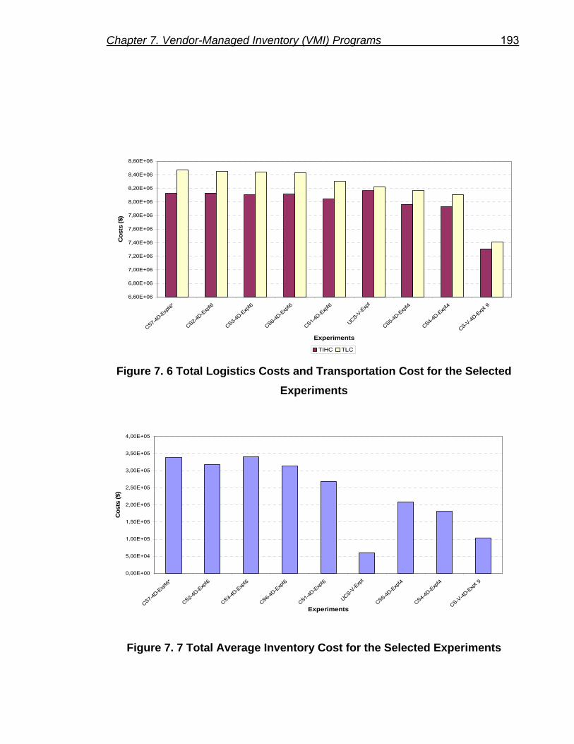
Chapter 7. Vendor-Managed Inventory (VMI) Programs 193
6,60E+06
6,80E+06
7,00E+06
7,20E+06
7,40E+06
7,60E+06
7,80E+06
8,00E+06
8,20E+06
8,40E+06
8,60E+06
CS7-4D-E
xpt6*
CS2-4D-E
xpt6
CS3-4D-E
xpt6
CS6-4D-E
xpt6
CS1-4D-E
xpt6
UCS-V-E
xpt
CS5-4D-E
xpt4
CS4-4D-E
xpt4
CS-V-4D
-Exp
t 9
Experiments
Cos
ts ($
)
TIHC TLC Figure 7. 6 Total Logistics Costs and Transportation Cost for the Selected
Experiments
0,00E+00
5,00E+04
1,00E+05
1,50E+05
2,00E+05
2,50E+05
3,00E+05
3,50E+05
4,00E+05
CS7-4D-E
xpt6*
CS2-4D-E
xpt6
CS3-4D-E
xpt6
CS6-4D-E
xpt6
CS1-4D-E
xpt6
UCS-V-E
xpt
CS5-4D-E
xpt4
CS4-4D-E
xpt4
CS-V-4D
-Exp
t 9
Experiments
Cos
ts ($
)
Figure 7. 7 Total Average Inventory Cost for the Selected Experiments

Chapter 7. Vendor-Managed Inventory (VMI) Programs 194
0,48%
12,43%
3,46%2,84%
1,87%
4,22%
0,00%
0,19% 0,27%
0%
2%
4%
6%
8%
10%
12%
14%
CS7-4D-E
xpt6*
CS2-4D-E
xpt6
CS3-4D-E
xpt6
CS6-4D-E
xpt6
CS1-4D-E
xpt6
UCS-V-E
xpt
CS5-4D-E
xpt4
CS4-4D-E
xpt4
CS-V-4D
-Exp
t 9
Experiments
Dec
reas
ing
TLC
Figure 7. 8 Percentage of Decreased Total Logistics Costs for the Selected
Experiments
From the previous table and the figures, the following conclusions can be made:
• The (UCS-V-Expt) strategy reduces the total logistics costs by
approximately 3% as compared to the CS7-4D-Expt6 strategy (Base).
• The CS-V-4D-Expt 9 strategy reduces the total logistics costs by
approximately 12% as compared to the CS7-4D-Expt6 strategy (Base).
• The CS-V-4D-Expt 9 strategy is the optimal strategy in terms of total
logistics costs. Furthermore, this strategy has the minimum transportation
cost as compared to all the strategies discussed in this thesis.
7.3.3. Truck Utilization Analysis
As mentioned in the analysis of the results of the UCS-V-Expt Strategy, the
transportation cost of the VMI-Programs uncoordinated strategy is higher than the
transportation cost of all the uncoordinated strategies in Chapter 4. To get a
deeper insight into the reason behind the increasing of the transportation cost in
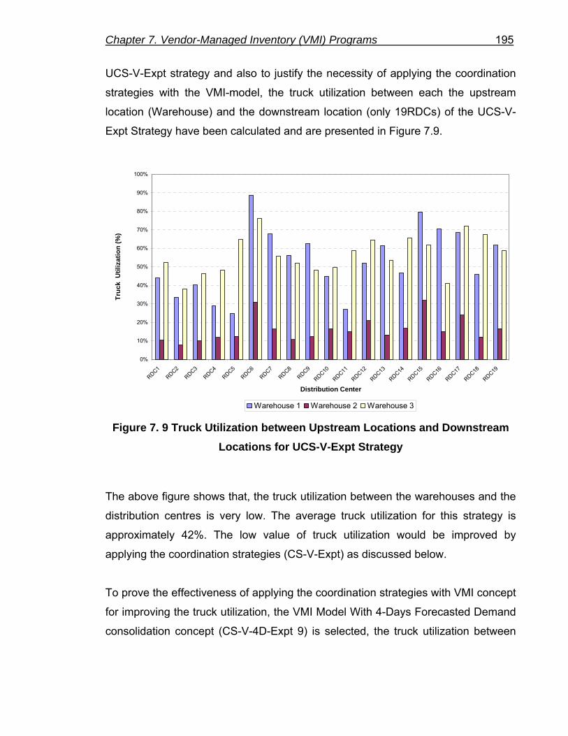
Chapter 7. Vendor-Managed Inventory (VMI) Programs 195
UCS-V-Expt strategy and also to justify the necessity of applying the coordination
strategies with the VMI-model, the truck utilization between each the upstream
location (Warehouse) and the downstream location (only 19RDCs) of the UCS-V-
Expt Strategy have been calculated and are presented in Figure 7.9.
0%
10%
20%
30%
40%
50%
60%
70%
80%
90%
100%
RDC1RDC2
RDC3RDC4
RDC5RDC6
RDC7RDC8
RDC9
RDC10
RDC11
RDC12
RDC13
RDC14
RDC15
RDC16
RDC17
RDC18
RDC19
Distribution Center
Truc
k U
tiliz
atio
n (%
)
Warehouse 1 Warehouse 2 Warehouse 3 Figure 7. 9 Truck Utilization between Upstream Locations and Downstream
Locations for UCS-V-Expt Strategy
The above figure shows that, the truck utilization between the warehouses and the
distribution centres is very low. The average truck utilization for this strategy is
approximately 42%. The low value of truck utilization would be improved by
applying the coordination strategies (CS-V-Expt) as discussed below.
To prove the effectiveness of applying the coordination strategies with VMI concept
for improving the truck utilization, the VMI Model With 4-Days Forecasted Demand
consolidation concept (CS-V-4D-Expt 9) is selected, the truck utilization between

Chapter 7. Vendor-Managed Inventory (VMI) Programs 196
each upstream location (Warehouse) and the downstream location (only 19RDCs)
have been calculated and presented in Figure 7.10 .
0%
10%
20%
30%
40%
50%
60%
70%
80%
90%
100%
RDC1RDC2
RDC3RDC4
RDC5RDC6
RDC7RDC8
RDC9
RDC10
RDC11
RDC12
RDC13
RDC14
RDC15
RDC16
RDC17
RDC18
RDC19
Distribution Center
Truc
k U
tiliz
atio
n (%
)
Warehouse 1 Warehouse 2 Warehouse 3
Figure 7. 10 Truck Utilization between Upstream Locations and Downstream Locations for CS-V-4D-Expt 9 Strategy
As can be seen from Figure 7.10, the 4-Days Forecasted Demand consolidation
concept can guarantee that the truck utilization in some cases is 100% (a full
truckload) and on average is more than 85%. The truck utilization of this strategy
(CS-V-4D-Expt 9) is approximately 43% higher than that of UCS-V-Expt Strategy.
7.3.4. Lower Bound Transportation Cost Analysis
As mentioned before, the CS-V-4D-Expt 9 strategy is the optimal strategy in terms
of total transportation costs (Table7.5). Furthermore, to investigate how much
(percentage) of the total transportation cost of this strategy is increased as
compared to the lower bound total transportation costs, an experiment is

Chapter 7. Vendor-Managed Inventory (VMI) Programs 197
conducted. In this experiment, the CS-V-4D-Expt 9 strategy is repeated under a
new assumption that it has the minimum transportation cost as compared to all the
strategies discussed so far. The assumption is due to the fact that the
transportation tariff (minimum cost) is offered for a full truck load between each
warehouse and distribution centre and it will be used as the transportation cost in
this experiment. The results of this experiment (Lower Bound Transportation Cost)
are compared with the results of the CS-V-4D-Expt 9 strategy and presented in
Table 7.6.
Table 7. 6 Measures of Performance of Lower Bound Transportation Cost Experiment
The results in the above table show that, the total transportation cost of the optimal
strategy (CS-V-4D-Expt 9) is approximately only 2% higher than the lower bound
transportation cost experiment. This means that, the optimal strategy (CS-V-4D-
Expt 9) achieves 98% of the lower bound of total transportation cost.
Conclusion: Referring to the above results and analysis, the following conclusions can be
made:
• In all cases the VMI approach performs better than the other coordination
strategies for optimizing supply chain performance.
• The VMI approach can efficiently reduces the inventory-carrying costs.
• The VMI approach with 4-Days Forecasted Demand consolidation concept is
an optimal coordination distribution strategy.
Experiments TTC TIHC TLCCS-V-4D-Expt 9 $7.310.720,73 $103.310,88 $7.414.031,61
Lower Bound Transportation Cost _Expt $7.193.362,65 $103.310,88 $7.296.673,53

Chapter 8. Conclusions and Future Work 198
8. Conclusions and Future Work
8.1. Conclusions
Throughout this dissertation, many conclusions have been made. These
conclusions are summarized as follows:
1- The correct selection of item classification (More Frequent Items) and
estimation of consolidated load for each item are the keys for getting the
optimal coordination strategy.
2- More frequent items should be included in all consolidated shipments.
3- The optimal size of the consolidated shipment for each item should be
between (20-80%) of consumption rate to increase the replenishment
interval time of more items with minimum residual stock.
4- The truck capacity should be allocated to all items so as to maximize the
time to next replenishment.
5- The classification of items is a tool for good design control strategy in
distribution problems.
6- A two or more dimensional classification approach can help in improving
the measure of performance as a very good strategy can be designed in
the supply chain.
7- The classification and allocation of items has effect on the total logistic
costs. Allocation of inventory strategies can give attractive savings on
total logistic cost especially when only the Item Fill Rate is considered.
8- More measures of performance should be used to give more insights on
the performance of the system and on the right decisions to be taken.
9- Well designed coordination strategy can perform better than
uncoordinated strategy and reduces the systemwide costs (logistic costs)
efficiently.

Chapter 8. Conclusions and Future Work 199
10- Understanding of residual stock behavior can help to achieve more
powerful coordination between the transportation and inventory functions
in supply chain management.
11- The developed consolidation concepts can guarantee that the order
quantities will generate a full truckload.
12- Companies have good opportunities to improve performance, to reduce
cost and to increase service level by coordinating the supply chain.
13- VMI concept would be convenient for the supply chain as a whole.
14- In complex systems with high demand variations, it is difficult to design
powerful distribution strategy.
15- More integration of information between upstream locations and
downstream locations is required. This helps to reduce the effect of
demand variations and make good forecasting to design very powerful
coordination strategy that would improve system performances.
16- Information availability is the key element for integration and coordination
the different supply chain stages.
17- Sharing of information among the supply chain partners is a fundamental
requirement for effective supply chain management.
18- It is clear that the implementation of advanced information technology
could reduce systemwide cost.
Industries realize that managing information flow is as important as managing
material flow in the supply chain. Simulation plays an important role for building
such complex integrated systems. Supply chains are too complicated to
analyze through analytical modeling. Simulation models can represent the
uncertainty, variability and coordinating problems in the supply chains in an
effective way.
19- Simulation is a powerful tool for studying supply chains.
20- Using simulation to evaluate supply chain strategies can lead to better
decisions, saving money, decreased inventory, and improved customer
service.

Chapter 8. Conclusions and Future Work 200
8.2. Future Work
There are many opportunities and several ways in which the various concepts
presented in this research can be extended in the future. These ways are:
• More complex and real transportation cost structures
• More experiments and strategies. For example, VMI approach with 6-Days
Forecasted Demand consolidation concept
• Different network structures
• More common inventory policies (echelon stock concept)
• Non-direct shipment between different locations (Vehicle Routing Problem)
• Optimal strategy for each downstream location to see the effect of
decentralization strategies on supply chain coordination
• More item classification criteria to make more sensitive analysis of item
characteristics which results in appropriate design of distribution and
coordination strategies
• New shipment consolidation concept that would combine the quantity and time
controlling criteria for designing the consolidated shipment
Further work has already been started and it is in the beginning stage of expanding
the simulation model presented in this study to investigate the application of non-
direct shipment and the impact of finding the right inventory policy with the vehicle
scheduling (Routing) rules on the performance of supply chains will be
investigated. This problem is called the Inventory Routing Problem (IRP) in the
literature.

Chapter 9. References 201
9. References [AF90] Anily, S. and Federgruen, A., 1990, “One warehouse multiple retailer
systems with vehicle routing costs,” Management Science, Vol.36,
No.1, pp. 92–114.
[AI88] Atkins, DR and P. Iyogun, 1988, "Periodic versus can-order policies
for coordinated multi-item inventory systems," Management Science,
Vol. 34, No. 6, pp. 791-796.
[AF98] Aviv, Y.,and Federgruen, A., 1998, “The operational benefits of
information sharing and vendor managed inventory (VMI) programs,”
Working paper, Washington University, St.Louis, MO.
[Axs00] Axsäter, S. 2000, “Inventory Control,” Kluwer Academic Publishers.
Boston, MA.
[BBE98] Bagchi S., Buckley S. J., Ettl M., and Lin G. Y., 1998, “Experience
using the IBM supply chain simulator,” Proceedings of the 1998
Winter Simulation Conference.
[Bal64] Balintfy, J., 1964, "On a basic class of multi-item inventory problems,"
Management Science, Vol. 10, No. 2, pp. 287-297.
[Bal04] Ballou, R. H., 2004, “Business Logistics/Supply Chain Management,”
5th Edition, Prentice Hall, Englewood Cliffs, NJ.
[BCN03] Banks, J., Carson, J.S., Nelson, B.L., and Nicol, D.M., 2003,”
Discrete-Event System Simulation,” 3rd Edition, Prentice Hall.

Chapter 9. References 202
[Bea98] Beamon, B.M., 1998,” Supply chain design and analysis: models and
methods,” International Journal of Production Economics, Vol. 55, pp.
281–294.
[Bha98] Bhaskaran, S., 1998, “Simulation analysis of a manufacturing supply
chain,” Decision Sciences, Vol. 29, No. 3, pp. 633-657.
[BCG93] Bhatnagar, R., Chandra, P. and Goyal, S. K., 1993, “Models for multi-
plant coordination,” European Journal of Operational Research, Vol.
67, pp. 141–160.
[Bre81] Brennan, J. J., 1981, “Models and analysis of temporal consolidation,”
Ph.D. Dissertation, University of California at Los Angeles, Los
Angeles, CA.
[BKS99] Bukowski L., Karkula M., and Schiff K.,1999, “Internal transport –
simulation applying Dosimis-3 package,” Logistics 6/99.
[BHB85] Burns, L.D., Hall, R.W., Blumenfeld, D.E. and Daganzo, C.F. , 1985,
“Distribution strategies that minimize transportation and inventory
costs,” Operations Research, Vol. 33, No. 3, pp. 469-490.
[CF97] Cachon, G.P., and Fisher, M., 1997, “Campbell soup’s continuous
replenishment program: evaluation and enhanced inventory decision
rules,” Production and Operations Management, Vol. 6, No. 3,
pp.266-276.
[CF00] Cachon, G., and Fisher, M., 2000,” Supply chain inventory
management and the value of shared information,” Management
Science, Vol. 46, pp. 1032–1048.

Chapter 9. References 203
[CM88] Carlson, ML and Miltenburg, J., 1988,"Using the service point model
to control large groups of items," Omega, Vol. 16, No. 5, pp. 481-489.
[CL00] Cetinkaya, S., and Lee, C. Y., 2000, “Stock replenishment and
shipment scheduling for vendor-managed inventory systems,”
Management Science, Vol. 46, pp. 217–232.
[CMS02] Chan, L. M. A., Muriel, A., Shen, Z.J., Simchi-Levi, D. and Teo, C.P.,
2002, “Effective zero-inventory-ordering policies for the single-
warehouse multiretailer problem with piecewise linear cost
structures,” Management Science, Vol. 48, No.11, pp. 1446–1460.
[Cha93] Chandra, P., 1993, “A dynamic distribution model with warehouse
and customer replenishment requirements,” Journal of the
Operational Research Society, Vol.44, No. 7, pp. 681-692.
[CC05] Chen, T. and Chen.J., 2005, “Optimizing supply chain collaboration
based on joint replenishment and channel coordination,"
Transportation Research Part E 41. pp. 425-441
[CL02] Cheung, K. L., and Lee, H. L., 2002, “The inventory benefit of
shipment coordination and stock rebalancing in a supply chain,”
Management Science, Vol. 48, No. 2, pp. 300-306
[CM04] Chopra, S., Meindl, P., 2004, “Supply Chain Management: Strategy,
Planning, and Operations,” 2nd Edition. Pearson Prentice Hall,New
Jersey.
[Chu03] Chu, Edward , 2003, “A review of simulation studies on supply chain
management,” Journal of Academy of Business and Economics.

Chapter 9. References 204
[CS60] Clark, A.J and Scarf, H., 1960, “Optimal policies of a multi-echelon
inventory problem,” Management Science, Vol. 6, pp. 475-490.
[DB87] Dror, M. and Ball, M., 1987, “Inventory/routing: reduction from an
annual to a short period,” Naval Research Logistics, Vol. 34, pp. 891-
905.
[DB03] Díaz, L., and Buxmann P., 2003, “The value of cooperative planning
in supply chains, a simulative approach,” The 11th European
Conference on Information Systems” (ECIS 2003), Naples, Italy. pp.
1-17.
[ESP98] Eliter, T., Subrahmanian, V.S., and Pick, G., 1998, “Heterogeneous
active agents,” Computer Science Technical Report Series, University
of Maryland, College Park.
[EB94] Elsayed, E. and Boucher, T.,1994, “Analysis and Control of
Production Systems,” Prentice Hall. 2nd. London.
[FGT84] Federgruen, A., Groenevelt, H., and Tijms, H.C. , 1984, “Coordinated
replenishments in a multi-item inventory system with compound
Poisson demands,” Management Science, Vol. 30, pp. 344-357.
[FZ84] Federgruen, A. and Zipkin, P. 1984, “A combined vehicle routing and
inventory allocation problem,” Operations Research, Vol. 32, No. 5,
pp. 1019-1037.
[FW87] Flores, B. E., Whybark, D.C., 1987, "Implementing multiple criteria
ABC analysis," Journal of Operations Management, Vol. 7, No. 1/2,
October.

Chapter 9. References 205
[GÖ01] Gallego G. and Özer , Ö. , 2001, " Integrating replenishment
decisions with advance demand information," Management Science,
Vol. 47, No. 10, pp. 1344-1360.
[GKT96] Gavirneni, S., Kapuscinski, R., and Tayur, S., 1996, “Value of
information in capacitated supply chains,” Working paper, Carnegie
Mellon University, Pittsburgh, PA.
[Goy73] Goyal, S.K., 1973, “Determination of economic packaging frequency
of items jointly replenished,” Management Science, Vol. 20, pp. 232-
235.
[Goy74] Goyal, S.K., 1974, “Determination of optimal packaging frequency of
jointly replenished items,” Management Science, Vol. 21, pp. 436-
443.
[GS89] Goyal SK and Satir AT., 1989, “Joint replenishment inventory control:
deterministic and stochastic models,” European Journal of
Operational Research, Vol. 38, pp. 2-13.
[GK01] Grabara, J. K., and Kot, S., 2001, “New tools of engineering
education for logistics training,” International Conference on
Engineering Education, Oslo, Norway.
[Hal87] Hall, R. W., 1987, “Consolidation strategy: inventory, vehicles and
terminals,” Journal of Business Logistics, Vol. 8, No. 2, pp. 57-73.
[HS99] Hamm, S., and Stepanek, M., 1999, “From re-engineering to e-
engineering,” Business Week (March 22) 62.

Chapter 9. References 206
[HB94] Higginson, J.K. and Bookbinder, J.H.,1994, “Policy recommendations
for a shipment consolidation program,” Journal of Business Logistics,
Vol. 15 No. 1, pp. 87-112.
[HB95] Higginson, J.K. and Bookbinder, J.H.,1995, “Markovian decision
processes in shipment consolidation,” Transportation Science, Vol. 29,
No. 3, pp. 242–255.
[HAN05] Housein, T. A., Aldarrat H. S., Noche, B., 2005, “Investigating the
effect of the integration of transportation strategies and inventory
policies on the performance of multi-echelon distribution systems,”
The First International Conference on Transportation Logistics, T-
LOG2005, Singapore.
[JWC01] Jain, S., Workman, R.W., Collins, L.M., and Ervin, E.C., 2001,
“Development of a high-level supply chain simulation model,”
Proceedings of the 2001 Winter Simulation Conference, pp. 1129-
1137.
[KSS02] Kelton, W.D., Sadowski, R.P., and Sadowski, D.A., 2002, “Simulation
with Arena,” 2nd Edition, McGraw-Hill.
[Knu03] Knut Alicke , 2003, “Planung und Betrieb von Logistiknetzwerken.
Unternehmensübergreifendes Supply Chain Management, ” Springer-
Verlag , Berlin, Heidelberg, New York.
[LGC05] Lambert, D. M., García-Dastugue, S. J., and Croxton, K. L., 2005, “An
evaluation of process-oriented supply chain management
frameworks,” Journal of Business Logistics, Vol. 26, No. 1, pp. 25-51.

Chapter 9. References 207
[LST00] Lee, H. L., So, K., and Tang, C. 2000, “The value of information
sharing in a two-level supply chain,” Management Science, Vol. 46,
No. 5, pp.626-643.
[Liu03] Liu, S., 2003, “On the integrated production, inventory, and
distribution routing problem,” Ph.D Thesis, The State University of
New Jersey, U.S.A.
[LY00] Liu, L. and Yuan, X., 2000, “Coordinating replenishments in inventory
systems with correlated demands,” European Journal of Operations
Research, Vol.123, pp. 490-503.
[MR03] Manuel D. Rossetti, Hin-Tat Chan., 2003, "A prototype object-oriented
supply chain simulation framework," Winter Simulation Conference,
pp. 1612-1620.
[MRF03] Mason, S.J., Ribera, MP., Farris, J. A. and Kirk, R. G., 2003,
“Integrating the warehousing and transportation functions of the
supply chain,” Transportation Research Part E, Vol.39, pp. 141–159.
[MDK01] Mentzer, J. T., DeWitt, W. J. , Keebler, J. S. , Min, S. , Nix, N. W. ,
Smith, C. D. , and Zacharia, Z. G. , 2001, "Defining supply chain
management," Journal of Business Logistics, Vol. 22, No. 2, pp. 1-25.
[Mil87] Miltenburg, J., 1987,"Co-ordinated control of a family of discount-
related items," INFOR, Vol. 25, No. 2, pp. 97-116.
[MS84] Miltenburg, G.J., and Silver, E.A., 1984, "The diffusion process and
residual stock in periodic review coordinated control of families of
items," International Journal of Production Research, Vol. 22, pp.
629-646.

Chapter 9. References 208
[MZ02] Min, H., and Zhou, G., 2002, “Supply chain modelling: past, present
and future,” Computer and Industrial Engineering, Vol. 43, pp. 231-
249.
[Mor00] Morales, M., 2000, “Optimization problems in supply chain
management,” Ph.D Thesis, Rotterdam University, Holland.
[Nil06] Nilsson, A. 2006, “Essays on joint replenishment and multi-echelon
inventory system,” Ph.D Thesis, Luleå University of Technology,
Department of Business Administration and Social Sciences, Division
of Industrial Logistics.
[NAH04] Noche, B., Aldarrat H. S., Housein, T. A., 2004, “Evaluating and
developing operating strategies in distribution networks using
simulation,” Experiences from the Future, Fraunhofer IRB-Verlag,
Tagungsband 11. ASIM-Fachtagung Simulation in ProduKtion und
Logistik, Berlin, pp. 75-84.
[NT01] Nozick, L. K., and Turnquist, M. A., 2001, “A two-echelon inventory
allocation and distribution center location analysis,” Transportation
Research E, Vol.37, pp. 425-441.
[Par96] Parker, K. 1996, “Demand management and beyond,” Manufacturing
Systems (June), 2A–14A.
[Pun02] Pundoor, G., 2002, “Supply Chain Simulation Models for Evaluating
the Impact of Rescheduling Frequencies,” MS 2002-9, Institute for
Systems Research, University of Maryland.
[RT02] Reiner, G. , Trcka, M. , 2002 ,“Supply Chain Management in the Food
Industry – Alternatives for a Production Company Analyzed by a

Chapter 9. References 209
Simulation Model,” 12th International Working Seminar on Production
Economics, Igls/ Innsbruck, Austria.
[SN99] Sarmiento, A.-M. and Nagi, R., 1999, “A Recent Directions in
Integrated Analysis of Manufacturing-Distribution Systems,” IIE
Transactions on Scheduling and logistics, special issue on
Manufacturing Logistics, Vol. 31, No. 11, pp. 1061-1074.
[SM98] Schenck, J., and McInerney, J. 1998, “Applying vendor-managed
inventory to the apparel industry,” Automat. I.D. News 14(6), pp. 36–
38.
[Sch01] Schulte, G. , 2001, “Material- und Logistikmanagement,” 2. Auflage (2th edition), Oldenbourg Wissenschaftsverlag GmbH.
[SP00] Schunk, D. and Plott, B., 2000. “Using simulation to analyze supply
chains,” In Proceedings of the 2000 Winter Simulation Conference.
ed. Joines, J.A., Barton, R.R., Kang, K., and Fishwick, P.A.,
Piscataway, New Jersey: Institute of Electrical and Electronic
Engineers, pp. 1095-1100.
[SJX04] Schwarz, L.B, James, W. and Xin, Z., 2004, “Joint transportation-and-
inventory problems in supply chains: A Review,” Working paper.
[SPP98] Silver, E.A. , Pyke, D.F, Peterson, R.,1998, “Inventory Management
and Production Planning and Scheduling,” 3rd Edition. John Wiley &
Sons, New York.
[SKS03] Simchi-Levi, Kaminsky, D. P., Simchi-Levi, E., 2003, “Designing and
Managing the supply chain: Concepts, Strategies and case studies,”
2nd Edition. McGraw Hill Higher Education, New York.

Chapter 9. References 210
[Sim99] Simison, R. L., 1999, “Toyota develops a way to make a car within
five days of a custom order,” Wall Street Journal (August 6).
[SPC03] Siprelle, A. J., Parsons, D. J., and Clark, R. J., 2003, “Benefits of
using a supply chain simulation tool to study inventory allocation,”
Processing of the 2003 Winter Simulation Conference, pp238-245.
[SRE05] Sombat , S., Romeijn, H. E., Akcali, E. , and Boondiskulchok, R.,
2005, “An integrated inventory-routing system for multi-item joint
replenishment with limited vehicle capacity,” Journal of Global
Optimization, Vol. 32, pp. 93–118.
[SB06] Stock, J.R., and Broadus, C. J., 2006, “Doctoral research in supply
chain management and/or logistics-related areas: 1999-2004,”
Journal of Business Logistics, Vol. 27, No. 1, pp. 139-496.
[SSS98] Swaminathan, J.M., Smith, S.F., and Sadeh, N.M., 1998, “Modeling
supply chain dynamics: a multiagent approach,” Decision Sciences,
Vol. 29, No. 3, pp. 607-631.
[TF99] Takakuwa, S. and Fujii, T., 1999, “ A Practical module-based
simulation model for transshipment-inventory systems,” In
Proceedings of the 1999 Winter Simulation Conference, ed. P. A.
Farrington, H. B. Nembhard, D. T. Sturrock, and G. W. Evans, pp.
1324-1332.
[Tan01] Tan, K.C., 2001, “A framework of supply chain management
literature,” European journal of purchasing & supply Management,
Vol. 7, Nr. 1, pp. 39-48.

Chapter 9. References 211
[TC04] Terzi, S. and Cavalieri,S., 2004, “Simulation in the supply chain
context: a survey,” Computers in industry, Vol. 53 Nr.1, 3-16.
[TG96] Thomas, D.J. and Griffin, P.M., 1996, “Coordinated supply chain
management,” European Journal of Operational Research, Vol. 94,
No. 1, pp. 1–15.
[VBB00] Van der Vorst, J.G.A.J., Beulens, A.J.M., and van Beek, P., 2000,
“Modeling and simulating multi-echelon food systems,” European
Journal of Operational Research, Vol.122, No. 2, pp. 354-366.
[VBW98] Van der Vorst, J. G. A. J. , Beulens, A. J. M. , de Wit, W., and van
Beek, P., 1998, “Supply chain management in food chains:
Improving performance by reducing uncertainty,” International
Transactions in Operational Research, Vol. 5, No. 6, pp. 487 – 499.
[VM97] Viswanathan, S. and Mathur, K., 1997, “Integrating routing and
inventory decisions in one-warehouse multiretailer multiproduct
distribution systems,” Management Science, Vol. 43, No. 3, pp. 294–
312.
[WJD99] Waller, M., Johnson, ME, and Davis, T. 1999, “Vendor managed
inventory in the retail supply chain,” Journal of Business Logistics,
Vol. 20, No.1, pp.183-203.
[Wat03] Waters, Donald ,2003, “ Global Logistics and Distribution Planning:
Strategies for Management,” 4th edition. Published by: Kogan Page
Limited, London.

Chapter 9. References 212
[XB06] Xu, Lei and Beamon, Benita M., 2006, “Supply chain coordination and
cooperation mechanisms: an attribute-based approach,” Journal of
Supply Chain Management, Vol. 42, No. 1, pp. 4-12.
[Yan00] Yang, K. K. ,2000, “Managing a single-warehouse, multiple-retailer
distribution system,” Business Logistics, Vol. 21, No. 2, pp. 162-172.

Curriculum Vitae Personal Data
Name: Tarak Ali Housein Sex: Male Date of Birth: 04 March 1969 Place of Birth Benghazi, Libya Marital Status: Married Nationality: Libyan Language: Arabic, English, German
Employment History:
2001 – 2006 PhD Researcher, Abteilung Maschinenbau, Institut für Transportsysteme und –logistik,Universität Duisburg-Essen, Germany
1996 – 2001 Assistant Lecturer; Department of Industrial Engineering,
Faculty of Engineering, Garyounis University, Libya
1995 – 1996 Project Planning Engineer, GREAT Man-made River Project 1993 –1995 Cost Engineer, Brown and Root Limited Company, Libya
Education and Qualification
2001 – 2006 PhD Degree in Mechanical Engineering, Universität Duisburg-Essen, Germany. 1991 –1997 M.Sc. Degree in Industrial Engineering Garyounis University, Libya 1986 – 1991 B.Sc. Degree in Industrial Engineering Garyounis University, Libya
Publication
2005 Housein, T. A., Aldarrat H. S., Noche, B., 2005,
“Investigating the effect of the integration of
transportation strategies and inventory policies on the
performance of multi-echelon distribution systems,” The
First International Conference on Transportation
Logistics, T-LOG2005, Singapore.
2005 Aldarrat H. S., Housein, T. A., Noche, B., 2005, “A
strategic supply chain simulation: distribution network
model description and prototype,” The First
International Conference on Transportation Logistics, T-
LOG2005, Singapore.
2004 Noche, B., Aldarrat H. S., Housein, T. A., 2004,
“Evaluating and developing operating strategies in
distribution networks using simulation,” Experiences
from the Future, Fraunhofer IRB-Verlag, Tagungsband
11. ASIM-Fachtagung Simulation in ProduKtion und
Logistik, Berlin.
1999 Shouman, M. A., Housein, T. A., 1999, “The combined
interactive process between material handling systems
and dispatching mechanisms in FMS,” Alexandria
Engineering Journal, Vol. 38, No. 1, Egypt.