Optimization of Nonlinear Dynamical ProblemsUsing Successive Linear Approximations in

LS-OPT

Nielen Stander? Rudolf Reichert?? Thomas Frank??

? Livermore Software Technology Corporation, Livermore, CA?? DaimlerChrysler, Stuttgart, Germany

Corresponding author:

Nielen StanderLivermore Software Technology Corporation7374 Las Positas RoadLivermoreCA 94550+1 925-449-2500nielen@lstc.com

Keywords:

Optimization, Parameter Identification, Response Surface Methodology, Struc-tural Optimization, System Identification

16-1

Abstract

This paper focuses on a successive response surface method for the optimiza-tion of problems in nonlinear dynamics. The response surfaces are built usinglinear mid-range approximations. To assure convergence, the method employstwo dynamic parameters to adjust the move limits. These are determined by theproximity of successive optimal points and the degree of oscillation, respective-ly. Three diverse examples namely in impact design, sheet metal process designand system identification are used to demonstrate the method. The methodolo-gy has been incorporated as a parallel solver in the commercial software codeLS-OPT.

INTRODUCTION

The Response Surface Method (Myers, 1995) has become a popular methodfor conducting optimization involving the simulation of nonlinear dynamicalproblems. The purpose of the method is primarily to avoid the necessity foranalytical or numerical gradient quantities as these are either too complex toformulate, discontinuous or sensitive to roundoff error. A common optimizationprocedure is to build a high order response surface in a region of interest in thedesign space and to refine the response surface in a semi-automated fashion bymoving the center of the region of interest as well as reducing its size. Such anapproach is suitable for making design improvements but not for problems suchas the parameter identification of systems or materials where a converged resultis desirable. Automated methods have therefore been formulated to addressproblems in rigid body dynamics (Etman, 1997) and sheet metal forming (Kok,1998), (LSTC, 1999). The method presented here incorporates sophisticatedfeatures into these approaches. These are:

� contraction of the region of interest to a reasonable, possibly irregulardesign space,

� the use ofD-optimal experimental design within an irregular design s-pace,

� the use of move characteristics to determine the contraction rate of theregion of interest and

� the identification of oscillation vs. ‘panning’ (translation of the region ofinterest in the design space) to determine the maximum shrinkage rate ofthe region of interest.

Nonlinear dynamic problems are particularly susceptible to random error ofwhich the degree is difficult or impossible to determine analytically. Hence the

16-2

approximation error has not been used to determine the dynamic parameters ofthe method.

APPROACH

Experimental designThe method presented here is based on the design of experiments. For experi-mental design theD-optimality criterion is used (Myers, 1995). The advantageof this criterion is that experiments can be chosen in an irregular design space(Kaufman, 1996). This feature is advantageous for two main reasons:

� Accuracy. If design constraints are chosen as bounds for the region ofinterest, the size of the region is reduced which is likely to give a moreaccurate result.

� Robustness. Non-robust or unreasonable designs can be avoided. Exam-ples can be found amongst designs with an unreasonably large mass ordesigns which may cause failure of the simulation process.

ApproximationsIn response surface methodology surfaces are fitted to the responses of the de-sign points determined by the experimental design. A common approximationmethod is the fitting of polynomials although other types of surfaces can also beused. Quadratic polynomials are usually accurate for a mid-range region of thedesign space but because the expense is a function ofn2 (wheren is the num-ber of design variables) they are normally avoided for large design problems.This applies particularly to nonlinear problems involving large finite elementmodels. A possible solution is to use linear approximations. These are gener-ally inaccurate beyond the immediate neighborhood of the design point but canbe used in a successive response surface procedure (Etman, 1997). The diffi-culty with using successive linear approximations is thatcyclingor oscillationmay occur. This phenomenon can be countered by manipulation of the size ofthe region of interest, a measure analogous to applying move limits in succes-sive linear programming. Heuristic measures are typically introduced (Etman,1997).

Successive response surface methodIn the following procedure, two parameters have been used to drive a successivelinear response surface method:

1. A maximum contractionparameter is determined based on whether thecurrent and previous designs are on opposite or the same side of the region

16-3

of interest. The former case signals the onset of oscillation while thelatter suggests that the optimum lies beyond the region of interest. Theparameter determines the maximum shrinkage rate and should thereforebe small for the oscillatory case and big for the ‘panning’ case.

2. An effective contractionparameter interpolates between the maximumcontraction parameter and a constant minimum contraction parameter us-ing the distance of the current optimum to the center of the region ofinterest as input.

Software: LS-OPTThe afore-mentioned methods have been incorporated in the program LS-OPT,a command language-based, standalone general optimization program whichis closely interfaced with LS-DYNA. Access to most quantities available inthe LS-DYNA database has been provided and maximum, minimum, averagedand filtered (see cylinder example) quantities can be automatically extracted.Special metal-forming quantities such as the forming limit criterion (FLD) arealso available. For shape optimization (Akkerman, 2000), a preprocessor can beincorporated in the design cycle. Job execution can be conducted in parallel andin a distributed fashion (Akkerman, 2000) using an additional module. Multi-case and multi-disciplinary optimization can be conducted.

EXAMPLES

In the present study, the iterative solver within LS-OPT has been applied tothe optimization of a diversity of problems in nonlinear dynamics using LS-DYNA. The purpose, in each example, is to use a remote, often unreasonableinitial design to test the robustness and efficiency and to assess the requirementfor a good starting design. A final tolerance of 1% has been set on the objectivefunction.

Three examples are used to illustrate the methodology implemented in LS-OPT.A fourth example, that of a vehicle crashworthiness optimization appears else-where in these proceeedings (Akkerman, 2000).

Airbag system identificationFive system parameters, representing the leakage properties of a deploying andimpacted airbag (Figure 1) are determined from the displacements, velocitiesand accelerations produced by two separate physical experiments. The leak-age properties are represented by a leakage vs. pressure curve defined by fiveunknown ordinates. The two experiments are distinguished by the velocity ofimpact namely 4 m/s and 5 m/s. Altogether 54 responses, 9 per time historycurve, are used in the regression. This represents a monitoring increment of 5ms.

16-4

The design requires amonotonicleakage curve. Some designs resulting froma standard experimental design may not have this property and may thereforecause the simulation to fail. Monotonicity of the experimental design can beenforced by using the constraints on the design variables:

xk+1 > xk; k= 1;2; :::;9 (1)

to relocate points in a new, irregular region. AD-optimal experimental design,using 17 points, is thus determined within a so called “reasonable design s-pace” (Kaufman, 1996) defined by the monotonicity constraints.D-optimalityis chosen as one of few possibilities for determining an experimental design inan irregular design space. To test the robustness of the algorithm, a constantnumber, 0.6, was chosen to represent the starting design for all variables. Thebounds [0.2,4] were applied uniformly with an initial range of 1.0. This startingpoint causes two designs to abort. In the first iteration the procedure thereforerelied on oversampling of the design space to simulate enough designs (8 out of10).

The objective of the problem is to minimize the discrepancy between the com-putational and experimental results, thereby effectively calibrating the compu-tational model. The RMS residual

R=

vuut 54

∑j=1

�f j(x)�Fj

Γ j

�2

(2)

is used as a measure of calibration accuracy. Since all quantities are in differentunits, they have been normalized using suitableΓ j . The symbolsFj representthe target values of the responses andf j the computational responses.

Figure 1: Airbag: Deployment, impact (33 ms) and rebound (50 ms)

16-5

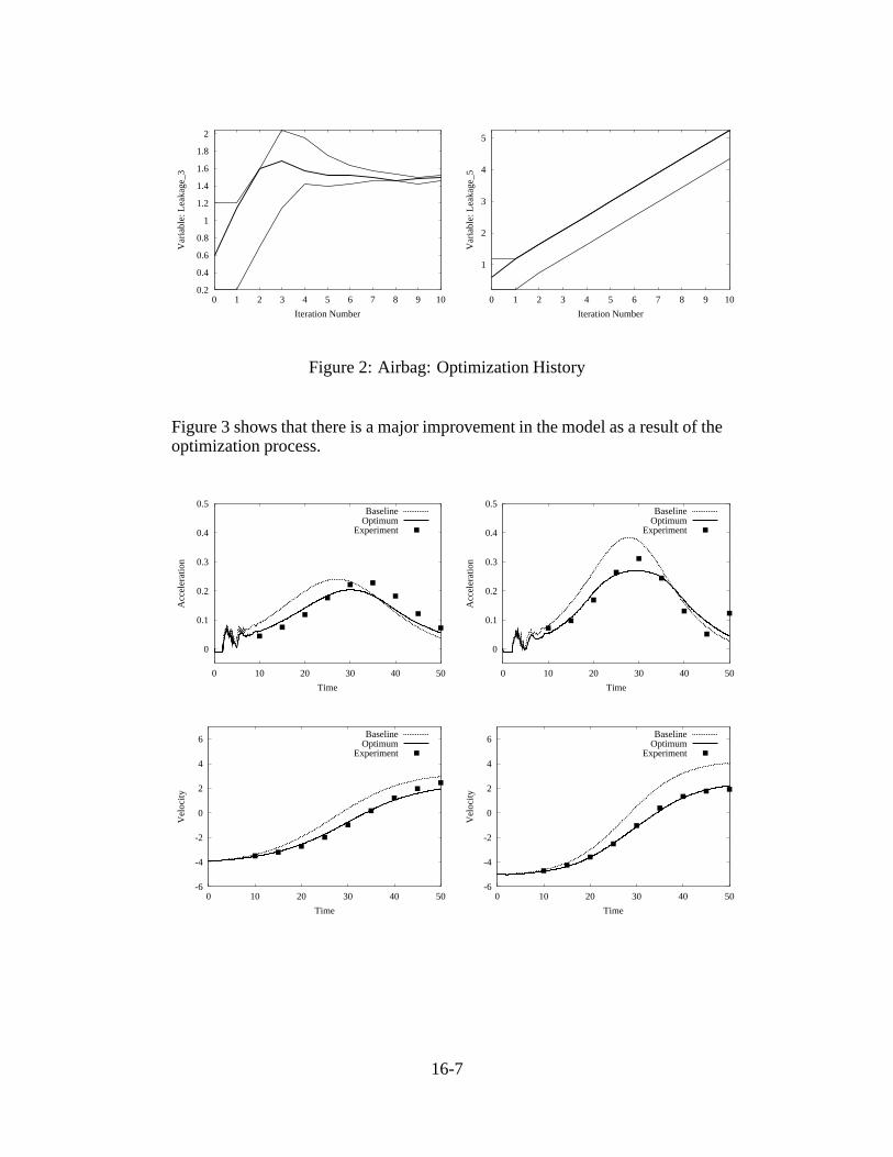
The optimization history (Figure 2) and the optimal design (Table 1) show thatalthough there are 5 design variables, some of them are constrained by themonotonicity, with the result that there are only three independent variables.

Table 1. Optimal leakage ordinates vs. pressure

Variable Pressure Leakagex1 2.0 0.361x2 2.25 1.492x3 2.5 1.492x4 2.75 1.492x5 3.0 5.25

The first variable oscillates while the last has not converged yet. However, judg-ing by the convergence properties of the residual and by the design sensitivities(not shown here) the smaller sensitivities of these two variables appear to renderthem insignificant in the neighborhood of the optimum.

1.5

2

2.5

3

3.5

4

4.5

5

5.5

0 1 2 3 4 5 6 7 8 9 10

Obj

ectiv

e: R

esid

ual

Iteration Number

0.2

0.4

0.6

0.8

1

1.2

1.4

1.6

0 1 2 3 4 5 6 7 8 9 10

Var

iabl

e: L

eaka

ge_1

Iteration Number

0.2

0.4

0.6

0.8

1

1.2

1.4

1.6

1.8

0 1 2 3 4 5 6 7 8 9 10

Var

iabl

e: L

eaka

ge_2

Iteration Number

16-6

0.2

0.4

0.6

0.8

1

1.2

1.4

1.6

1.8

2

0 1 2 3 4 5 6 7 8 9 10

Var

iabl

e: L

eaka

ge_3

Iteration Number

1

2

3

4

5

0 1 2 3 4 5 6 7 8 9 10

Var

iabl

e: L

eaka

ge_5

Iteration Number

Figure 2: Airbag: Optimization History

Figure 3 shows that there is a major improvement in the model as a result of theoptimization process.

0

0.1

0.2

0.3

0.4

0.5

0 10 20 30 40 50

Acc

eler

atio

n

Time

BaselineOptimum

Experiment

0

0.1

0.2

0.3

0.4

0.5

0 10 20 30 40 50

Acc

eler

atio

n

Time

BaselineOptimum

Experiment

-6

-4

-2

0

2

4

6

0 10 20 30 40 50

Vel

ocity

Time

BaselineOptimum

Experiment

-6

-4

-2

0

2

4

6

0 10 20 30 40 50

Vel

ocity

Time

BaselineOptimum

Experiment

16-7

-90

-80

-70

-60

-50

-40

-30

-20

-10

0

0 10 20 30 40 50

Dis

plac

emen

t

Time

BaselineOptimum

Experiment

-120

-100

-80

-60

-40

-20

0

0 10 20 30 40 50

Dis

plac

emen

t

Time

BaselineOptimum

Experiment

Figure 3: Airbag: Comparison of computational and experimental results

Sheet metal form designA sheet metal problem (Figure 4) is presented in which themaximumradius ofthe cross-sectional die geometry has to be minimized.

Figure 4: Finite Element model of tools and blank

Three design variables, the outer three radii of the cross-section of the die, havebeen chosen. The constraints are the forming limit criterion (zero is the bound-ing value) and the maximum thinning of 20%. Mesh adaptivity is used duringanalysis to improve the curvature of the deformed model (shown with a coarsemesh in Figure 4). A detailed description of the problem can also be found inthe LS-OPT User’s Manual (LSTC, 1999).

16-8

The initial radii are chosen as 1.5mm uniformly and the final results are shownin Figure 5. The history results show that the thinning and FLD responsesconverge in about 2 iterations. Two or three further iterations are required tominimize the maximum of the three radii. A violation of the bounds of theregion of interest occurs in the first iteration because a feasible design could notbe found and therefore the bounds are compromised by the core optimizationsolver. Figure 6 shows the baseline and optimal flow limit diagrams with thedegree of violation clearly visible for the baseline case.

1

1.5

2

2.5

3

3.5

0 1 2 3 4 5 6 7 8

Var

iabl

e: R

adiu

s_1

Iteration Number

1

1.2

1.4

1.6

1.8

2

2.2

2.4

2.6

2.8

0 1 2 3 4 5 6 7 8V

aria

ble:

Rad

ius_

2

Iteration Number

1.2

1.3

1.4

1.5

1.6

1.7

1.8

1.9

2

0 1 2 3 4 5 6 7 8

Var

iabl

e: R

adiu

s_3

Iteration Number

20

25

30

35

40

0 1 2 3 4 5 6 7 8

Res

pons

e: T

hinn

ing

Iteration Number

0

0.05

0.1

0.15

0.2

0.25

0 1 2 3 4 5 6 7 8

Res

pons

e: F

LD

Iteration Number

Figure 5: Metal forming: optimization history

16-9

-0.2

0

0.2

0.4

0.6

0.8

1

-1 -0.5 0 0.5 1

Maj

or S

trai

n

Minor Strain

FLD-diagram (baseline)

Curve 90

-0.2

0

0.2

0.4

0.6

0.8

1

-1 -0.5 0 0.5 1

Maj

or S

trai

n

Minor Strain

FLD-diagram (Optimal)

Curve 90

Figure 6: Baseline and optimal flow limit diagrams

Impact optimizationThe problem, based on (Yamazaki, 1997), consists of a tube impacting a rigidwall as shown in Figure 7. The energy absorbed is maximized subject to aconstraint on the maximum rigid wall impact force. The cylinder has a constantmass of 0.54 kg with the radius and thickness as design variables. The length ofthe cylinder is dependent on the design variables because of the mass constraint.A concentrated mass of 500 times the cylinder weight is attached to the end ofthe cylinder not impacting the rigid wall. The deformed models are shown inFigure 8.

The optimization problem is stated as:

MaximizeEinternal(x1;x2)jt=0:05

subject toFwall

normal(x1;x2)jmax� 100,000

l(x) =0:52

2πρx1x2

where the design variablesx1 and x2 are the radius and the thickness of thecylinder respectively.Einternal(x)jt=0:05 is the objective function and constraintfunctionsFwall

normal(x)jmax and l(x) are the maximum normal force (filtered withSAE 300Hz) on the rigid wall and the length of the cylinder respectively.

16-10

l

x2

10 m/s

x1

Figure 7: Impacting cylinder

Figure 8: Deformed configurations: (a) Baseline (t = 50ms) and (b) Optimal(t = 50ms)

The optimization history (Figure 9) shows that the initial design is severelyinfeasible but that the design evolves to be feasible after two iterations. Thereduction of the force coincides with an increase in absorbed energy. The dataof the optimal design are given in Table 2.

16-11

Table 2. Starting values, bounds and optimal values

Variable Start Lower Optimum UpperBound Bound

Radius 75 30 30 100Thickness 3 2 4.7 6Internal energy 12,490 13,360Peak Wall force 1,544,000 109,100 100,000

Figure 10 confirms the feasibility of the design with three of the force peaksbeing active. It is apparent that the baseline design is too soft, causing a suddenlarge force peak upon contact of the trailing mass with the wall. The optimaldesign has a more evenly distributed force with a small violation of about 9%.

0

2

4

6

8

10

12

14

0 1 2 3

Res

pons

e: R

igid

_Wal

l_Fo

rce

Iteration Number

1.22

1.24

1.26

1.28

1.3

1.32

0 1 2 3

Res

pons

e: I

nter

nal_

Ene

rgy

Iteration Number

2

2.5

3

3.5

4

4.5

5

5.5

6

0 1 2 3

Var

iabl

e: W

all_

Thi

ckne

ss

Iteration Number

30

40

50

60

70

80

90

100

0 1 2 3

Var

iabl

e: R

adiu

s

Iteration Number

Figure 9: Cylinder: Optimization History

16-12

0

50000

100000

150000

200000

0 0.01 0.02 0.03 0.04

Rig

id W

all F

orce

(N

)

Time (sec)

OptimumBaseline

Figure 10: Cylinder: Constrained rigid wall force:F(t)� 100;000 (SAE300Hz filtered)

SUMMARY

The computational effort of the above examples is summarized in Table 3. Thenumbers are based on the stopping criterion of a 1% change of the objectivefunction. Because of the direct use of the design variables in the objective ofthe sheet metal problem, the tolerance has been relaxed to 3%. The final checksimulation and case multiplicity (airbag problem) are included in the numbersof the last column.

Table 3. Summary of Computational Data

Problem type Variables Simulations/it. It. SimulationsAirbag 5 10 10 101�2Sheet-metal Die 3 7 8 57Cylinder 2 5 3 16

The methodology has also been validated by the larger problem with 11 designvariables (Akkerman, 2000). That problem requires 3 iterations employing 58simulations in total (19 each).

16-13

CONCLUSIONS

An adaptive successive response surface method which employs the conver-gence properties in conjunction with a ‘reasonable’ experimental design proce-dure is shown to provide a high degree of accuracy, robustness and efficiencyfor optimization. Starting from a remote and often unreasonable initial design,an optimal design of reasonable engineering accuracy can be obtained rapidly.Linear approximations make the approach effective for a large number of de-sign variables. The methodology is suitable for a wide range of problems innonlinear dynamics and is highly accurate, as is often required for parameteridentification problems.

REFERENCES

AKKERMAN, A., BURGER, M., KUHN, R., RAJIC, H., STANDER, N. andTHYAGARAJAN, R. (2000). Shape optimization of instrument panel compo-nents for crashworthiness using distributed computing, Proceedings of the 6thLS-DYNA User’s Conference, Dearborn, MI, April 9-11, 2000.

ETMAN, P. (1997). Optimization of Multibody Systems using ApproximationConcepts. Ph.D. thesis, Technical University Eindhoven, The Netherlands.

KAUFMAN, M.D. (1996). Variable-Complexity Response Surface Approxi-mations for Wing Structural Weight in HSCT Design. M.S. thesis, VirginiaPolytechnic Institute and State University.

KOK, S. and STANDER, N. (1998). Optimization of a Sheet Metal FormingProcess using Successive Multipoint Approximations. AIAA paper 98-2301,39th AIAA/ ASME/ ASCE/ AHS/ ASC Structures, Structural Dynamics andMaterials Conference, Long Beach, CA, April 20-23, 1998.

LSTC (1999). LS-OPT User’s Manual, Livermore Software Technology Cor-poration, September, 1999

MYERS, R. and MONTGOMERY, M. (1995). Response Surface Methodology– Process and Product Optimization Using Designed Experiments, Wiley, NewYork.

YAMAZAKI, K., HAN, J., ISHIKAWA, H. and KUROIWA, Y. (1997). Maxi-mization of Crushing Energy Absorption of Cylindrical shells - simulation andexperiment, Proceedings of the OPTI-97 Conference, Rome, Italy, September1997.

16-14