optimised sensor configurations for a maglev suspension ... · optimised sensor configurations for...
TRANSCRIPT
FACTA UNIVERSITATIS Series: Mechanics, Automatic Control and Robotics Vol. 6, Special Issue, 2007, pp. 169 - 184
OPTIMISED SENSOR CONFIGURATIONS FOR A MAGLEV SUSPENSION SYSTEM
UDC 681.586:519.863(045)=111
Konstantinos Michail, Argyrios C. Zolotas, Roger M. Goodall
Department of Electronic and Electrical Engineering, Loughborough University, Loughborough, England, United Kingdom
e-mail: k.mihail; a.c.zolotas; g.m.goodall @lboro.ac.uk
Abstract. This paper discusses a systematic approach for selecting the minimum number of sensors for an Electromagnetic suspension system that satisfies both optimised deterministic and stochastic performance objectives. The performance is optimised by tuning the controller using evolutionary algorithms. Two controller strategies are discussed, an inner loop classical solution for illustrating the efficacy of the evolutionary algorithm and a Linear Quadratic Gaussian (LQG) structure particularly on sensor optimisation.
Key words: Sensor optimisation, MAGLEV suspensions, EMS optimisation, genetic algorithms, Kalman filter, evolutionary algorithms
1. INTRODUCTION
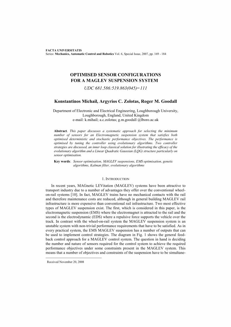
In recent years, MAGnetic LEVitation (MAGLEV) systems have been attractive to transport industry due to a number of advantages they offer over the conventional wheel-on-rail systems [10]. In fact, MAGLEV trains have no mechanical contacts with the rail and therefore maintenance costs are reduced, although in general building MAGLEV rail infrastructure is more expensive than conventional rail infrastructure. Two most effective types of MAGLEV suspension exist. The first, which is considered in this paper, is the electromagnetic suspension (EMS) where the electromagnet is attracted to the rail and the second is the electrodynamic (EDS) where a repulsive force supports the vehicle over the track. In contrast with the wheel-on-rail system the MAGLEV suspension system is an unstable system with non-trivial performance requirements that have to be satisfied. As in every practical system, the EMS MAGLEV suspension has a number of outputs that can be used to implement control strategies. The diagram in Fig. 1 shows the general feed-back control approach for a MAGLEV control system. The question in hand is deciding the number and nature of sensors required for the control system to achieve the required performance objectives under some constraints present in the MAGLEV system. This means that a number of objectives and constraints of the suspension have to be simultane- Received November 20, 2008
170 K. MICHAIL, A. C. ZOLOTAS, R. M. GOODALL
ously satisfied by varying the controller’s parameters for every feasible sensor set avail-able. Clearly, this is not an easy task especially if the system has many outputs to select from.
Fig. 1 Block diagram of typical MAGLEV suspension feedback control system
The work presented in this paper discusses a systematic framework for sensor optimisation applied to a quarter-car magnetic suspension model, which aims to satisfy both disturbance rejection and robustness to parametric changes as well as the best ride quality with minimum possible effort using lowest possible number of sensors from the available sensor sets. In fact, the problem is posed in a multiobjective optimisation frame-work to optimise the controller’s parameters, via a heuristic algorithm [4], for each avail-able sensor set.
Evolutionary algorithms are widely used in control engineering and have proved to be very efficient for controller optimisation in a number of problems in control systems [5]. Numerous genetic algorithms have been developed [1], although for the purposes of this work a recently developed genetic algorithm named Non-dominated Sorting Genetic Algorithm (NSGA-II) [3] is selected. The NSGAII principle is based on non-dominated sorting of the individuals in the chromosome and it is merged into the systematic frame-work to optimise the performance of the MAGLEV for every possible sensor set. In particular, the efficacy of NSGAII tuning is illustrated on a classical structure with inner-loop, while a Linear Quadratic Gaussian (LQG) structure is further utilised as the modern control approach for the systematic framework presented.
The paper is organised as follows: The linear time invariant state space model of a quarter car is presented in section 2 along with all possible sensor combinations. Section 3 presents the various inputs to the MAGLEV suspension, together with the objectives and numerous constraint limitations. Section 4 discusses the multiobjective constraint optimisation using evolutionary algorithms and section 5 the classical control optimisa-tion. Section 6 presents the proposed systematic framework while conclusions are drawn in section 7.
2. LINEARISED MAGLEV SUSPENSION MODEL
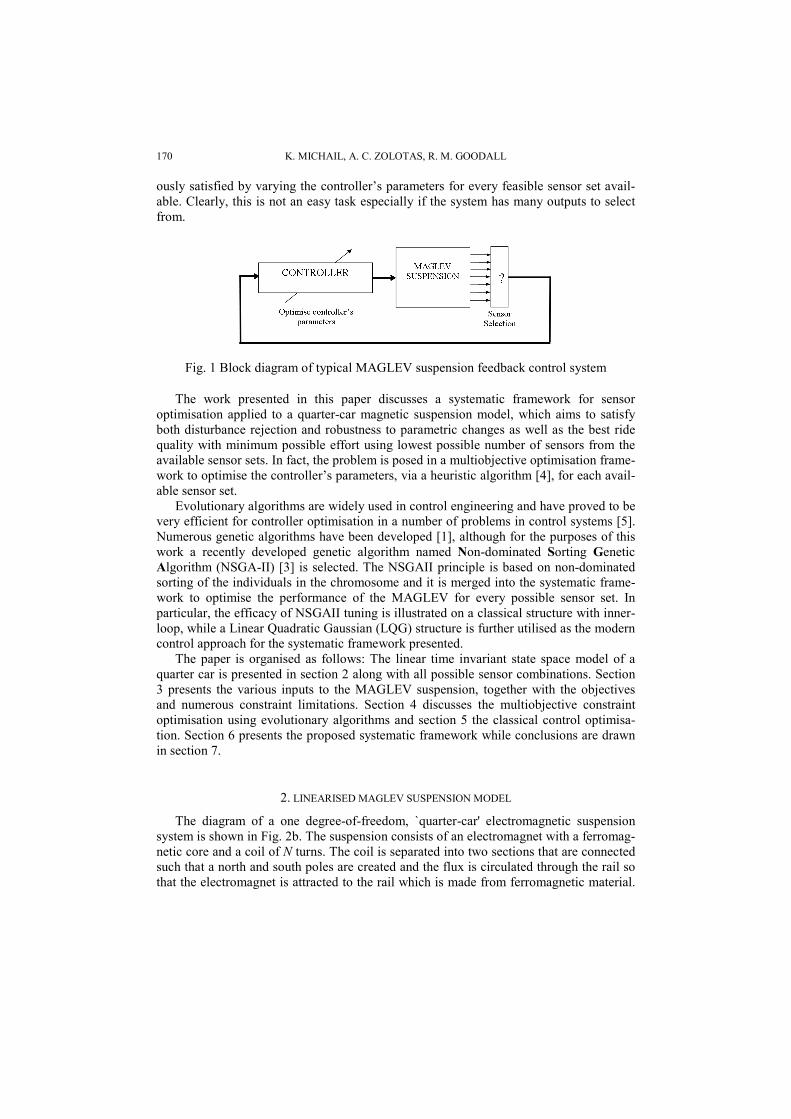
The diagram of a one degree-of-freedom, `quarter-car' electromagnetic suspension system is shown in Fig. 2b. The suspension consists of an electromagnet with a ferromag-netic core and a coil of N turns. The coil is separated into two sections that are connected such that a north and south poles are created and the flux is circulated through the rail so that the electromagnet is attracted to the rail which is made from ferromagnetic material.
Optimised Sensor Configurations for a Maglev Suspension System 171
The carriage mass is attached on the electromagnet, with zt the rail position and z the electromagnet position. The air gap (zt − z) is to be maintained close to the operating condition as required. Details are shown on the end view illustrated in Fig. 2a.
Fig. 2a Fig. 2b
Fig. 2 Diagram of an EMS
The LTI state space model is derived by considering small variations around the operating point (nominal) values of the coil current Io, flux density Bo, attractive force Fo and air gap Go as follows
oot
oo
IiIGzzGBbBFfF
+=+−=+=+=
)( (1)
where f, b, i and (zt − z) are small variations around the equilibrium point. The fundamen-tal magnetic relationships are F ∝ B2 and B ∝ I / G, thus, the linearised expressions for the magnet are derived from (initially) Goodall, 1985 [9] and more recently Goodall, 2008 [13] )()( zzKiKb tzzi t
−−= − bKf b= (2)
where Ki = Bo / Io, K(zt − z) = Bo / Go and Kb = 2Fo / Bo. The voltage u is given by
dtdbNA
dtdiLRiu ++= (3)
where N is the number of coil turns, R the coil resistance, A the pole face area and L the coil inductance. Moreover, the force f depends on the mass M and the vertical acceleration
..z .
..zMf = (4)
substituting flux and force equations in (2) into (4) the acceleration z&& is given as
)()(..zz
MKK
iM
KKz t
zzbib t −−= − (5)

172 K. MICHAIL, A. C. ZOLOTAS, R. M. GOODALL
from the flux equation in (2) and (3) the current equation is
i
t
i
zz
i NAKLRizz
NAKLNAK
NAKLu
dtdi t
+−−
++
+= − )(
..)( (6)
and from (5) and (6) a state vector with the corresponding states is selected as ])([ zzzix t −= & .
The state space equation is expression is given by
tz
ug zBuBxAxt
..
.++= , xCy m= (7)
where the state matrix Ag, the input matrix Bu, the disturbance matrix t
.z
B and the output
matrix Cm are given as follows:
⎟⎟⎟⎟⎟⎟⎟
⎠
⎞
⎜⎜⎜⎜⎜⎜⎜
⎝
⎛
−
−
+−
+−
= −
−
010
0
0
)(
)(
MKK
MKK
NAKLNAK
NAKLR
A zzbib
i
zz
i
gt
t
,
⎟⎟⎟⎟⎟⎟
⎠
⎞
⎜⎜⎜⎜⎜⎜
⎝
⎛+
=00
1
i
u
NAKLB (8)
⎟⎟⎟⎟⎟⎟
⎠
⎞
⎜⎜⎜⎜⎜⎜
⎝
⎛
+=
−
10
)(
i
zz
z
NAKLNAK
B
t
t&,
⎟⎟⎟⎟⎟⎟⎟
⎠
⎞
⎜⎜⎜⎜⎜⎜⎜
⎝
⎛
−
−
=
−
−
MKK
MKK
KK
C
zzbib
zzi
m
t
t
)(
)(
0
010100
0001
(9)
Note that the output matrix Cm here gives the five possible measurements y = [current (i), flux (b), air gap (zt − z), vertical velocity (
.z ), vertical acceleration (
..z )]T. The parame-
ter values for a one ton suspension system are shown in Table 1.
Table 1 MAGLEV suspension parameters
Carriage Mass ( M ) 1000kg Nominal force ( oF ) 9810N
Nominal air gap ( oG ) 0.015m Coil’s Resistance ( R ) 10Ω
Nominal flux density ( oB ) 1T Coil’s Inductance ( L ) 0.1H
Nominal current ( oI ) 10A Number of turns ( N ) 2000 Pole face area ( A ) 0.01m2

Optimised Sensor Configurations for a Maglev Suspension System 173
2.1. Sensor Combinations available
The sensor combinations available depend on the output matrix Cm in (9). The total number of sensor combinations (or sensor sets) is easily calculated from 12 −= sn
sN where Ns is the total number of all feasible sensor sets and ns the number of the total sen-sors that can be used. Table 2 shows the available sensor sets with 1,2,3,4 and 5 sensors that results to a total of 31 sensor sets. Note that the sensor sets will be used for for the LQG control but not for the classical approaches.
Table 2 Number of sensor sets available
Number of measurements available
Number of feasible sensor sets
With 1 sensor 5 With 2 sensors 10 With 3 sensors 10 With 4 sensors 5 With 5 sensors 1
3. INPUT DISTURBANCE AND PERFORMANCE REQUIREMENTS
3.1 Input disturbances
Two track input characteristics are considered, i.e. deterministic changes such as gradients or curves and stochastic (random) changes in the track position due to misalign-ments during installation. In particular,
3.1.1 Random Inputs to the MAGLEV suspension
Random behaviour of the rail position is caused as the vehicle moves along the track by track-laying inaccuracies and steel rail discrepancies. Considering the vertical direc-tion, the velocity variations are quantified by a double-sided power spectrum density (PSD) which in the frequency domain is expressed by
vrz VASt
π=& (10)
where Vv is the vehicle speed (in this work is taken as 15m/s) and Ar represents the track roughness equal to 1x10⁻⁷ (typical value for high quality track). The corresponding (one-sided) autocorrelation function is given by
)(2)( 2 τδπτ vrVAR = (11)
and a more detailed analysis on stochastic description of track irregularities is found in [12].
3.1.2 Deterministic Inputs to the MAGLEV suspension
The main deterministic inputs to a suspension for the vertical direction are the transi-tions onto gradients. In this work, the deterministic input components utilised are shown in Fig. 3 and represent a gradient of 5% at a vehicle speed of 15m/s, with a transition to give an acceleration of 0.5m/s2 and a jerk of 1m/s3.

174 K. MICHAIL, A. C. ZOLOTAS, R. M. GOODALL
Fig. 3 Deterministic input to the suspension with a vehicle speed of 15m/s and 5% gradient
3.2 Design requirements
Fundamentally there is a trade off between the deterministic and the stochastic re-sponse (ride quality) of the suspension. For slow speed vehicles, performance require-ments are described in [6] and [7]. In particular, the practical objective is to minimize both the vertical acceleration (improve ride quality) and the attractive force applied from the electromagnets by minimizing the RMS current variations. These objectives, noted as φ1 and φ2, can be formally written as in (12) and the constraints are listed in Table 3.
rmsi=φ1 and rmsz..
2 =φ (12)
4. MULTIOBJECTIVE CONSTRAINT OPTIMISATION VIA GENETIC ALGORITHMS
The problem is clearly posed into multiobjective constraint optimisation that can be solved with the Non-dominated Genetic Algorithm II (NSGAII). More details for this type of genetic algorithm are given in [3]. NSGAII is used in both classical and LQG controller structures for tuning, although with different constraints and parameters. The parameters used are shown in Table 4.
Table 3. MAGLEV suspension limitations
Constraints Value RMS acceleration ( g%5≈ ), ( rmsz&& ) <0.5ms-2 RMS gap variation, ((zt − z)rms) <5mm Air gap deviation (deterministic), ((zt − z)p) <7.5mm Control effort (deterministic), (up) <300V(3IoRo) Settling time (ts) <3s

Optimised Sensor Configurations for a Maglev Suspension System 175
The crossover probability is generally selected to be large (90%) in order to have a good mixing of genetic material. The mutation probability is defined as 1/nu, where nu is the number of variables. This is appropriate in order to give a mutation probability that mutates an average of one parameter from each individual. The number of variables is different for each optimisation problem as shown on Table 4. except from the simulated binary crossover parameter (SBX) and the mutations parameter it was decided to use the values of 20 and 20 in all cases since they provide good distribution of solutions for the algorithm operations. The population and generation sizes are set to 50 and 500 respec-tively for the classical controller optimisation and LQR tuning. Note that the LQR design serves as the ideal control performance for assessing the LQG design for every feasible sensor set.
Table 4 NSGAII parameters
Parameter Classical LQR LQG Crossover probability 0.9 0.9 0.9 Mutation probability 1/nu (nu = 5) 1/nu (nu = 4) 1/nu (nu = 1) Population (Popnum) 50 50 25 Generations (Gennum) 500 500 5
LQG tuning is more straightforward, as there is only one variable (i.e, process noise matrix (W) is the variable discussed in section (6)) to tune (Popnum=25, Gennum=5). There is no systematic method to define those values as they depend on the nature of the prob-lem. In fact, these values can be selected after a few trials or from experience. The more complicated the optimisation problem is, the higher the population number and the more generations are required. Moreover, the algorithm performance depends on the search space, i.e if it is too large the aforementioned generations and population may not be enough. In this work, the search space for both classical and LQG is decided after manu-ally designing an initial controller. To achieve the limitations described in Table 3 the penalty function approach [2] is used. The constraint violation for each constraint, ki de-fined in Table 3, is given as
0)()(
0)(<
=ωii
iikgif
otherwisekg
ij k (13)
Each constraint is normalized as in (14) for values less than the predefined and in (17) for values greater than the predefined.
01≥+−= ides
i
j kkg (14)
01 ≥−= ides
i
kkg j (15)
Where, idesk is the desired constraint value and ki is the measured value.
The overall constraint violation is taken as
∑=
ω=Ωj
j
ij
i kk1
)()( )()( (16)

176 K. MICHAIL, A. C. ZOLOTAS, R. M. GOODALL
The overall constraint violation is then added to each of the objective functions value l
)()()( )()()( im
im
im kRkk Ω+φ=Φ (17)
Where, Rm is the penalty parameter and φm(k(i)) the objective function value.
5. CLASSICAL CONTROLLER OPTIMISATION
Inner loop control is advantageous in controlling a MAGLEV vehicle [8]. Two controller structures are introduced in this section. A classical solution comprising an air gap outer-loop with flux inner-loop is compared with an air gap outer-loop with current inner-loop. The scheme is depicted in Fig. 4 for the air gap-flux case. The diagram also applies for the air gap-current case by replacing flux with current measurement.
The aims of the classical solution are 1) to demonstrate the effectiveness of the selected genetic algorithm 2) to compare the optimised performance for the two inner loop approaches 3) and to serve as a baseline for further investigation of schemes with more sensor
combinations. The tuning procedure is then extended in an LQG framework which is specifically
connected to appropriate sensor selection. A fixed set of classical compensators is considered, namely a proportional plus inte-
gral for the inner loops and a phase advance for the outer loop. The controller parameters are tuned simultaneously via the evolutionary algorithm NSGA-II in an attempt to opti-mise the control system performance subject to all constraints being satisfied. The inner loop bandwidth must be within 50Hz-100Hz while the outer loop is chosen less than 10Hz. A phase advance (PA) (18), with k the advance ratio and τ the time constant, is used to provide adequate phase margin in the range 35o-40o.
st
stGPIi
ii
1+= ,
11
+τ+τ
=sskGPA o (18)
Fig. 4 Classical controller impementation with flux inner loop feedback
Figure 5 depicts the Pareto-optimality between the ride quality z&& and the RMS coil current irms for the two controller configurations, i.e. the air gap-flux ((zt − z), b) and the air gap-current ((zt − z), i) case. It can be seen that a set of controllers can be chosen which satisfy all constraints for the ((zt − z), b) case but not for the ((zt − z), i), (more complex controller are necessary in the latter).

Optimised Sensor Configurations for a Maglev Suspension System 177
This can be seen in Table 5, where both case deterministic and stochastic responses are satisfied for all controllers for the ((zt − z), b) case. Robustness to parameter variations is considered only for the ((zt − z), b) configuration since the ((zt − z), i) configuration already violates two of the predefined constraints. A set of optimal controllers for the extreme cases of 2
..37.0 −= msz and 0.45ms-2 is selected, i.e. (19) is the first set of
controllers (C1) and (20) is the second set (C2). The mass (M) is varied by ±25% from the nominal value of M = 1000kg, for the dynamical system.
Table 5 Classical control – constraint values for each design
Constraint (zt − z) − b (zt − z) − i PM(degree) 35-45 35-40 6.5-7
)(Hzfoutb <10 3.2-3.8 ≈5.8
)(Hzfoutb 50-100 76-99 ≈100
Air gap peak (mm) <7.5 ≈5 ≈1 RMS air gap (mm) <5 ≈1.5 ≈1.5 Control effort (up) <300 ≈10 ≈30
RMS ..z (ms-2) <0.5 0.35-0.45 ≈0.98
Fig. 5 Pareto front of controllers for (zt − z), b (empty dots) and (zt − z), i (dark dots)
1015.01084.05.5,
018.01021.0116841 11 +
+=
+=
ssPA
ssPIC (19)
1016.01115.06.5,
018.01018.0100632 22 +
+=
+=
ssPA
ssPIC (20)
178 K. MICHAIL, A. C. ZOLOTAS, R. M. GOODALL
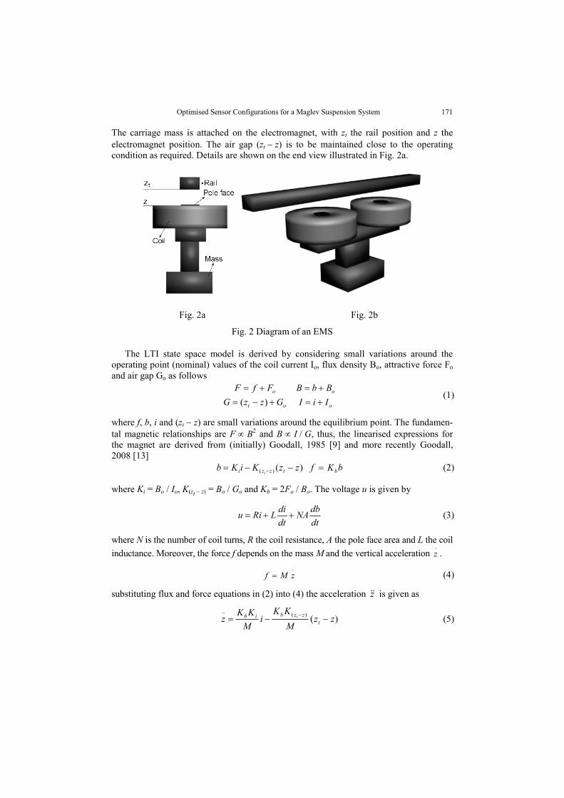
The effect of the mass variations is reflected to the constraints where small variations from the nominal performance occur. Table 6 shows the resulting constraint values for a ±25% mass variation. For the C1 controller it can be seen that the mass variations are accommodated and stability is maintained with small variation on the phase and the gain margins (similarly for the C2 case). In the case of C1 no constraint is violated for 25% mass variation but for the C2 controller set, being closer to the limits of the constraints, fails to satisfy the ride quality (vertical acceleration) requirement for the case where mass is 750kg. The deterministic disturbance (response to 5% track gradient) is successfully rejected in less than 3s and the steady state value of the air gap returns to the operating point (operating condition of 15mm). Of course, one might use the nominal model refer-ring to the worse case mass uncertainty at the expense of more conservative solutions for the lower uncertainty cases.
6. SENSOR OPTIMISATION VIA LQG
Linear Quadratic Gaussian control is well documented in the literature of control sys-tems [11], and thus its theoretical details are omitted.
Table 6 Constraints values for PI1 and PA1 at ±25% mass variation
M=750kg M=1000kg M=1250kg C1 C2 C1 C2 C1 C2 PM(degree) 38.2 49.9 35 44.7 32 42.7 fbin(Hz) 4 4.9 3.2 3.8 2.8 3.22 fbout(Hz) 95 84 95 84 95 84 Air gap peak (mm) 3.6 3.4 4.9 4.6 6.3 5.9 RMS air gap (mm) 1.3 1.18 1.71 1.27 1.87 1.34 RMS z&& )( 2−ms 0.47 0.61 0.37 0.44 0.3 0.36 Control effort (up) 25.88 24 35 33 45 42 Settling time (ts) 2.27 2.11 2.51 2.32 2.63 2.37
Consider the following state space expression utilised for designing the Liner Quad-ratic Gaussian controller (LQR and Kalman filter parts.
dwBBuxAx ω++=.
, nCxy ω+= (21)
where, the state matrix A = Ag, the input matrix B = Bu, the disturbance matrix .
tzw BB = and the output matrix C = Cm. All matrices are evaluated in equations (8), and (9).
Note that ωd and ωn are the process and measurement noises respectively. These are uncorrelated zero-mean Gaussian stochastic processes with constant power spectral densities W and V respectively. In particular, the problem is to find u = Klqg(s)y which minimises the performance index in (22) for every sensor set combination available (this particularly relates to the information provided to the Kalman filter).

Optimised Sensor Configurations for a Maglev Suspension System 179
][1lim0∫τ
∞→τ+
τ= dtRuuQxxEJ TT
LQG (22)
Here, Q and R are the state and control weighting functions respectively with Q = QT ≥ 0 and R = RT ≥ 0 of the Linear Quadratic Regulator part of the LQG controller.
For the LQR design we choose output regulation, i.e. regulate acceleration ..z , air gap
(zt − z) and the integral of air gap ∫(zt − z) (the last quantity specifically refers to the speed of response relating to achieving zero steady state error for the air gap). Thus, Q is in fact given by zz
Tz CQCQ = (23)
where Cz is the output matrix selecting the above regulated signals, i.e. T
tt zzzzz ])()([..
∫ −− and Qz is the corresponding weighting matrix. Both Q and R are tuned to recover the Pareto front of controllers that gives the optimum trade off between irms and
..z while satisfying the
preset constraints. The Kalman filter is designed such that ]ˆ[]ˆ[ xxxxE T −− is minimised via choosing W and V. Therefore, a desired response is selected from the LQR design which can be considered as the optimum performance, which is what the Kalman tuning aims to achieve via W and V tuning for every sensor set.
The scheme is shown in Fig. 6 with all possible measurements included. For appropri-ate disturbance rejection, i.e. zero steady state error for the air gap signal, the LQR part is designed on an augmented system with the extra integral state of the air gap (however the Kalman filter is designed on the original state space matrices, but the integral state is later provided by an appropriately chosen selector matrix Ci).
Fig. 6 Sensor optimisation via LQG
The measurement noise weighting (V) is constant and given in (24) for all sensors (If available this can be found from sensor equipment data sheets, but here is derived from prior simulation of baseline controller designs): the noise covariance matrix is con-structed by taking 1% of the peak from each measurement from the deterministic re-sponse of the suspension. In this design the process noise matrix
tzw BB &= and the process

180 K. MICHAIL, A. C. ZOLOTAS, R. M. GOODALL
noise covariance refers to the track velocity input. The W weighting matrix is the variable to be tuned for the 31 sensor sets that are available as described in section 2. The objective functions to be minimised for the deterministic (Φdet) and for the stochastic (Φstoch) responses are given in equation (25).
),,,,( )( zzzzbi VVVVVdiagVt &&&−= (24)
dtxxt
ao∫ −=φ0
det , )(stoch ao xxrms −=φ (25)
where, xo are the monitored states of interest of the closed loop with the LQR state feed-back (e.g. ideal closed loop) and xa the monitored states of interest of the closed loop with the overall LQG controller (e.g. actual closed loop prior to adding sensor noise). Note that the sensor information entering the Kalman filter is affected by sensor noise. This makes a total of 6 individual objective functions. The selection procedure of the Kalman estimator that satisfy the desired requirements is based on the overall penalty parameter (26), which is zero if all constraints are satisfied, and close to zero if the constraints are almost satisfied (see equation (16)). The next criterion is the sum of the objective func-tions given as
∑=
φφ=6
1stochdet ),(
iS (26)
When the optimisation procedure is finished, for each sensor set, the final population is assessed and the individual(s) that result(s) to the smallest overall penalty parameter in equation (16) are selected, and among these the individual (Kalman estimator) that gives the smallest S in equation (26) is the preferred choice.
The algorithm for the systematic framework developed is summarised as follows Step 1: Initialise algorithm by setting the NSGAII parameters and the performance re-quirements (i.e. objectives and constraints) of the suspension. Step 2: Tune the LQR controller and select the desired performance to be used as the ‘ideal’ performance for the Kalman estimator tuning. Step 3: Select a sensor set and check for observability/controllability via modal test. Step 4: Tune the Kalman estimator to achieve the ‘ideal’ LQR response for the cur-rent sensor set. Step 5: Select the best controller using equations using Ω and S . Step 6: Repeat steps 3-5 until all sensor sets are covered and save results.
The final choice for the minimum number of sensors can be followed in an appropri-ate manner.
The state feedback tuning recovers a Pareto front that is depicted in Fig. 7. In these re-sults a small relaxation to the deflection limit is considered (maximum air gap deflection allowed is 7.3mm) to accommodate the sensor noise effects in the next stage of the Kalman filter design. It can be easily seen that the ride quality is within limits and the current is around 1A. All controllers satisfy the preset constraints and therefore there are 50 control-lers to choose from. Figure 7 assists in choosing the LQR gain vector which has gains of
AVKuir /596
,= , 1/8375
,−= msVK
uzr&, mVK
uztzr /520992),(
−=−
, mVKuztzr /80936
),(−=
∫ −.
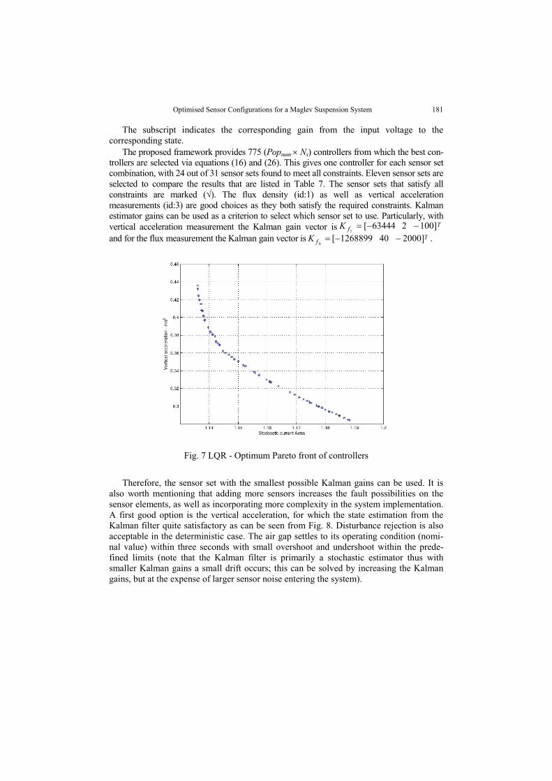
Optimised Sensor Configurations for a Maglev Suspension System 181
The subscript indicates the corresponding gain from the input voltage to the corresponding state.
The proposed framework provides 775 (Popnum × Ns) controllers from which the best con-trollers are selected via equations (16) and (26). This gives one controller for each sensor set combination, with 24 out of 31 sensor sets found to meet all constraints. Eleven sensor sets are selected to compare the results that are listed in Table 7. The sensor sets that satisfy all constraints are marked (√). The flux density (id:1) as well as vertical acceleration measurements (id:3) are good choices as they both satisfy the required constraints. Kalman estimator gains can be used as a criterion to select which sensor set to use. Particularly, with vertical acceleration measurement the Kalman gain vector is Tfz
K ]100263444[ −−=&&
and for the flux measurement the Kalman gain vector is Tfb
K ]2000401268899[ −−= .
Fig. 7 LQR - Optimum Pareto front of controllers
Therefore, the sensor set with the smallest possible Kalman gains can be used. It is also worth mentioning that adding more sensors increases the fault possibilities on the sensor elements, as well as incorporating more complexity in the system implementation. A first good option is the vertical acceleration, for which the state estimation from the Kalman filter quite satisfactory as can be seen from Fig. 8. Disturbance rejection is also acceptable in the deterministic case. The air gap settles to its operating condition (nomi-nal value) within three seconds with small overshoot and undershoot within the prede-fined limits (note that the Kalman filter is primarily a stochastic estimator thus with smaller Kalman gains a small drift occurs; this can be solved by increasing the Kalman gains, but at the expense of larger sensor noise entering the system).

182 K. MICHAIL, A. C. ZOLOTAS, R. M. GOODALL
Table 7 Comparison table for 11 sensor sets
id Sensor Set
rmst zz )( − (mm)
pt zz )( − (mm)
pu
(V) z&&
(ms-2) st
(s)
1 b 1.4 5.3 94 0.35 2.25 √ 2 )( zzt − 1.4 4.8 81 0.35 6.43 x 3 z&& 1.4 5.3 92 0.34 2.12 √ 4 zi &, 1.4 5.6 101 0.35 6.17 x 5 zi &&, 1.4 5.3 72 0.34 2.25 √ 6 )(,, zzbi t − 1.4 5.2 66 0.35 2.25 √ 7 zbi &,, 1.4 5.7 70 0.35 2.3 √ 8 zzzi t &),(, − 1.4 5.5 88 0.35 6.22 x 9 zzzbi t &),(,, − 1.4 5.6 63 0.35 2.3 √
10 zzzbi t &&),(,, − 1.4 5.3 65 0.35 2.2 √ 11 zzzzbi t &&&,),(,, − 1.4 5.5 63 0.35 2.2 √
Fig. 8 State estimation with vertical acceleration measurement

Optimised Sensor Configurations for a Maglev Suspension System 183
7. CONCLUSION
The paper discussed a system study from a sensor optimisation point of view for a magnetic suspension system via a heuristic approach (NSGAII) on controller tuning. Two controller cases were presented: A classical one uses fixed sensor sets for illustrating the efficacy of the heuristic algorithm on controller tuning. The second case discussed an LQG controller design with the particular aim of sensor optimisation for the Kalman fil-ter part. The study illustrated that most of sensors sets are able to provide satisfactory control of the magnetic suspension system. Note that the study identifies the minimum sensor sets required for appropriate performance, effectively reducing sensor fault scenar-ios. In particular, the presented framework aims to identify potential sensor sets that can be used as a basis for future investigation on system fault tolerance via possible controller structure reconfiguration.
Acknowledgement: This work was supported in part under the EPSRC (UK) project Grant Ref. EP/D063965/1 and BAE Systems (SEIC), UK.
REFERENCES 1. Abdullah, K., Coit, B.W., Smith, A.E.,2006, Multi-objective optimization using genetic algorithms: A
tutorial, Reliability Engineering and systems safety, page992-1007 2. Deb, K.,2001, Multi-objective Optimization Using evolutionary algorithms, John Wiley & sons Ltd 3. Deb, K., Pratap,A., Agarwal, S., Meyarivan T., 2002, A fast and Elitist Multiobjective Genetic Algorithm:
NSGA-II, IEEE transactions on evolutionary computation, volume 6, No2, pages 182—197. 4. Dreo, J., Siarry, P., Petrowski, A., Taillard, E., 2006, Metaheuritics for Hard Optimization, -Verlg Berlin
Heidelberg. 5. Flemming, P.J, Purshhouse, R.C., 2002, Evolutionary algorithms in control systems engineering: a sur-
vey, Control Engineering Practice page1223-1241. 6. Goodall, R.M., 1994, Dynamic characteristics in the design of Maglev suspension, IMechE, volume 208,
pages 33—41 7. Goodall, R.M., 2004, Dynamics and control requirements for EMS Maglev suspensions, Proceedings on
International Conference on Maglev, volume , pages 926-934 8. Goodall, R.M., 2000, On the robustness of flux feedback control for electro-magnetic Maglev controllers,
Proceedings of 16th International. Conference on Maglev systems and linear drives, page197-202. 9. Goodall, R.M., 1985, The theory of electromagnetic levitation, Physics in technology, Vol. 16, No5,
page207-213. 10. Lee, H.W., Kim, K.C., Lee, J., 2006, Review of Maglev Train Technologies, IEEE transactions on
magnetics, vol. 42, pages 1917-1925. 11. Skogestad, S., Postlethwaite., I, 2005, Multivariable feedback control - Analysis and design, Wiley &
Sons Ltd. 12. Paddison, J.E, 1995, Advance control strategies for MAGLEV suspension systems, PhD thesis, Loughbor-
ough University, United Kingdom. 13. Goodall, R.M., 2008, Generalised design models for EMS maglev, Proceedings of MAGLEV 2008 – The
20th International Conference on Magnetically Levitated Systems and Linear Drives.

184 K. MICHAIL, A. C. ZOLOTAS, R. M. GOODALL
OPTIMALNA SENZORSKA KONFIGURACIJA ZA MAGLEV LEVITACIONI SISTEM SUSPENZIJE
Konstantinos Michail, Argyrios C. Zolotas, Roger M. Goodall
Ovaj rad se bavi sistematskim pristupom u odabiranju minimalnog broja senzora za sistem elektromagnetne levitacione suspenziju koji zadovoljava obe ciljeve determinističke i stohastičke optimalne performanse. Performansa je optimalna podešavanjem upravljanja uz pomoć razvojnih algoritama. Proučavaju se dve strategije upravljanja, unutrašnja petlja klasičnog rešenja za ilustraciju efikasnosti razvojnih algoritama i Linearne Kvadratne Gausijeve (LQG) strukture posebno za optimizaciju senzora.
Ključne reči: Optimizacija senzora, MagLev suspenzija, EMS optimizacija, genetski algoritmi, Kalmanov filter, razvojni algoritmi