optimisation of running strategies according to ...fiorini.perso.math.cnrs.fr/semjeuneslmv.pdf ·...
TRANSCRIPT

Optimisation of running strategies according to physiological parameters
5/2/2016 - Séminaire des Doctorants
Camilla Fiorini

Camilla Fiorini 5/2/2016 /29
Aim
2

Camilla Fiorini 5/2/2016 /29
Mathematical framework
Ordinary differential equation:
+ n initial (or final) conditions
f(y(n)(t), y(n�1)(t), . . . , y(t), t;p) = 0state
p vector of parametersy
Direct problem:
Inverse problem (parameter identification):
p
p, f+ n i.c. SOLVE y
y, f+ n i.c.
IDENTIFY
3

Camilla Fiorini 5/2/2016 /29
Mathematical framework
Optimal control problems
u
f(y(n)(t), y(n�1)(t), . . . , y(t), u(t), t;p) = 0 u controlState equation:
Cost functional: J(u) = g(y(u)) quantity to be minimised
There can be n+1 initial (or final) condition.
The aim is to find u J(u) = minu2U
J(u)such that
subject to the state equation and the i.c.
yp, f, J
n+1 cond.OPTIMISE
4

Camilla Fiorini 5/2/2016 /29
Introduction
States:position velocity energy
x(t)
v(t)
e(t)
Control: propulsive force f(t)
Cost functional: final time T
Equations:
8><
>:
x(t) = ?
v(t) = ?
e(t) = ?
5

Camilla Fiorini 5/2/2016 /29
Introduction
States:position velocity energy
x(t)
v(t)
e(t)
Control: propulsive force f(t)
Cost functional: final time T
Equations:
8><
>:
x(t) = ?
v(t) = ?
e(t) = ?
v(t)
5

Camilla Fiorini 5/2/2016 /29
Introduction
Energy
Propulsive forceFriction
6

Camilla Fiorini 5/2/2016 /29
Keller’s model (1974)Equations:
Physiological constraints:
Optimisation problem:
subject to (1) and (2).
(1)
(2)
Matches the world records times
Unreasonable velocity profile No competition with other runners
Straight line
e(t) � 0, 0 f(t) fM 8t � 0.
minf2F
T (f)
8><
>:
x(t) = v(t) x(0) = 0, x(T ) = D
v(t) = f(t)� v(t)⌧ v(0) = 0
e(t) = � � f(t)v(t) e(0) = e
0.
7

Camilla Fiorini 5/2/2016 /29
Oxygen uptake (VO2)
� 6= const.
.
e(t) = � � f(t)v(t)
�(e)
8

Camilla Fiorini 5/2/2016 /29
Two-runners model
Slipstream
Psychological factor
8>>>>>><
>>>>>>:
x1 = v1 x1(0) = 0
x
D
= v2 � v1 x
D
(0) = 0
v1 = f1 � v1⌧1
� cv
21(1� �(e�↵(xD��)2)) v1(0) = 0
v2 = f2 � v2⌧2
� cv
22(1� �(e�↵(xD+�)2)) v2(0) = 0
e
i
= �
i
(ei
)� f
i
v
i
e
i
(0) = e
0i
.
1
0.2
11
1-γ
β0 2β
9
Camilla Fiorini 5/2/2016 /29
Two-runners model
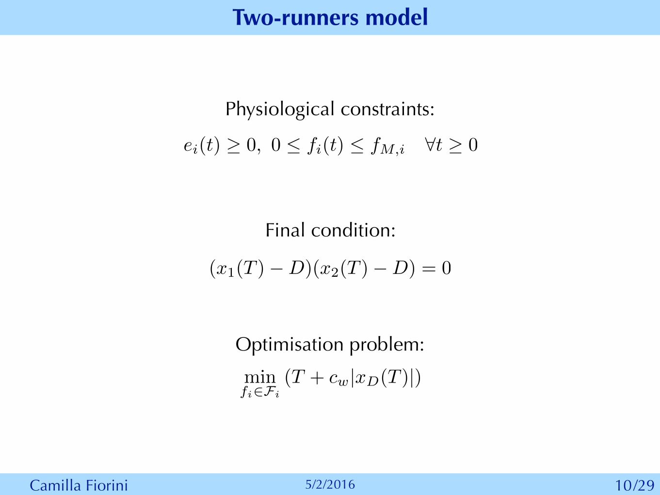
Physiological constraints:
ei(t) � 0, 0 fi(t) fM,i 8t � 0
Final condition:
(x1(T )�D)(x2(T )�D) = 0
Optimisation problem:
minfi2Fi
(T + cw|xD(T )|)
10

Camilla Fiorini 5/2/2016 /29
Curved path
Rcg
Rf
↵
(i) Leaning towards the centre
(ii) Increase of internal friction
(iii) Decrease of maximal force
11

Camilla Fiorini 5/2/2016 /29
(i) Leaning towards the centre
Curved path
x(t)xcg(t)xf (t)feet
centre of gravityv(t)vf (t)vcg(t)
xf (0) = 0, xf (T ) = DInitial and final conditions:
Newton’s second law: vcg(t) = f(t)� vcg(t)
⌧
xf (t) = vf (t) = h(vcg)
12

Camilla Fiorini 5/2/2016 /29
(i) Leaning towards the centre
Curved path
vfvcg
=Rf
Rcg
N cos↵ = mg N sin↵ = mv2cgRcg
) tan↵ =
v2cggRcg
sin2 ↵ =tan2 ↵
1 + tan2 ↵) sin↵ =
v2cg
gRcg
q1 +
v4cg
(gRcg)2
xf = vcg
0
@1 +Lv
2cg
Rcg
q(gRcg)2 + v
4cg
1
A
13
= 1 +L
Rcgsin↵
Rf �Rcg = L sin↵ , Rf
Rcg= 1 +
L
Rcgsin↵

Camilla Fiorini 5/2/2016 /29
(ii) Increase of internal friction
Curved path
⌧ = ⌧0(1� ⌧c tan↵) = ⌧0
✓1� ⌧c
v2
gRcg
◆
(iii) Decrease of maximal force
fM = fM,0(1� fc tan↵) = fM,0
✓1� fc
v2
gRcg
◆
14

Camilla Fiorini 5/2/2016 /29
Curved path
One runner model
tr(x) =
(0 if x 2 S1 if x 2 B
8>>>><
>>>>:
x
f
= v
✓1 + tr(x
f
) Lv
2
Rcg
p(gRcg)2+v
4
◆x
f
(0) = 0, x
f
(T ) = D
v = f � v
⌧0
⇣1�tr(xf )⌧c
v2gRcg
⌘ � cv
2v(0) = 0
e = �(e)� fv e(0) = e
0,
15
e(t) � 0, 0 f(t) fM,0
✓1� fc
v2
gRcg
◆

Camilla Fiorini 5/2/2016 /29
Curved path for two runners
Problem: definition of xD(t)
16
Camilla Fiorini 5/2/2016 /29
x
APPi,L (t) =
8>>>><
>>>>:
R1#0,L + R1RL
xi,L(t) if xi,L(t) 2 Ba,L
xi,L(t) + #0,LRL � ⇡(RL �R1) if xi,L(t) 2 Sa,L
R1RL
xi,L(t) +R1#0,L + L
⇣1� R1
RL
⌘if xi,L(t) 2 Bb,L
xi,L(t) if xi,L(t) 2 Sb,L
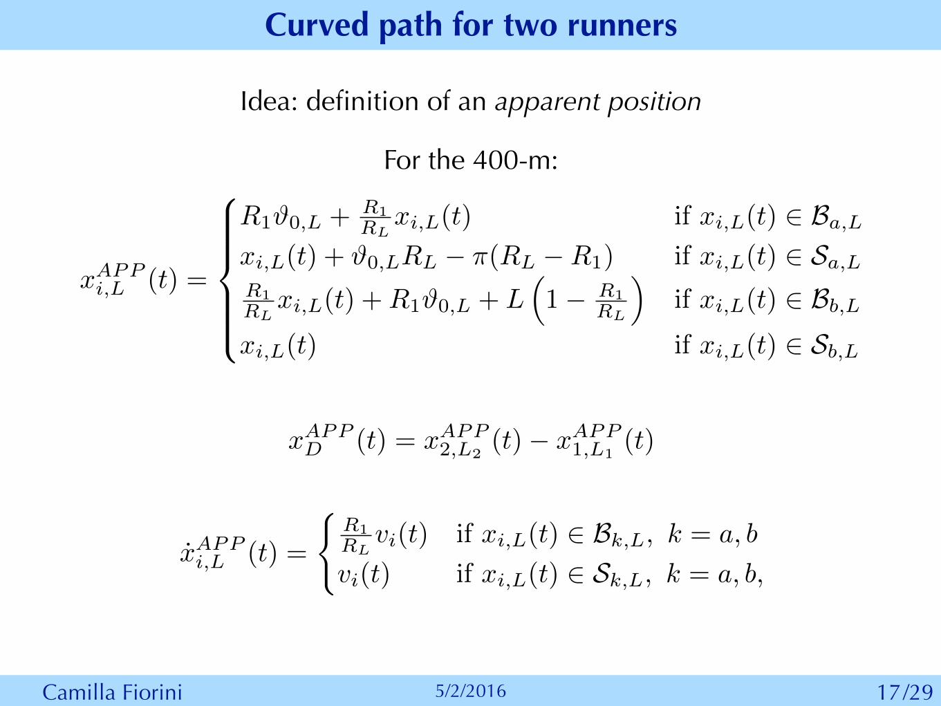
Curved path for two runners
Idea: definition of an apparent position
For the 400-m:
x
APPD (t) = x
APP2,L2
(t)� x
APP1,L1
(t)
x
APPi,L (t) =
(R1RL
vi(t) if xi,L(t) 2 Bk,L, k = a, b
vi(t) if xi,L(t) 2 Sk,L, k = a, b,
17

Camilla Fiorini 5/2/2016 /29
Curved path for two runners
Final model:
8>>>>>>>>><
>>>>>>>>>:
x1 = v1
✓1 + tr(x1)
Lv
21
Rcg
p(gRcg)2+v
41
◆x1(0) = 0
x
APP
D
= x
APP
2,L2� x
APP
1,L1x
APP
D
(0) = R1 (#0,L1 � #0,L2)
v1 = f1 � v1
⌧1
⇣1�tr(xf )⌧c
v2gRcg
⌘ � cv
21(1� �(e�↵(xAPP
D ��)2)) v1(0) = 0
v2 = f2 � v2
⌧2
⇣1�tr(xf )⌧c
v2gRcg
⌘ � cv
22(1� �(e�↵(xAPP
D +�)2)) v2(0) = 0
e
i
= �
i
(ei
)� f
i
v
i
e
i
(0) = e
0i
,
18
ei(t) � 0, 0 fi(t) fM,0,i
✓1� fc
v2
gRcg
◆
Camilla Fiorini 5/2/2016 /29
Numerical results
t[s]0 50 100 150 200 250
-1
0
1
2
3
4
5
6
7v[m/s]
fM
=5 N/kg
fM
=4.75 N/kg
fM
=5.25 N/kg
t[s]0 50 100 150 200 250
3.5
4
4.5
5
5.5f[N/kg]
fM
=5 N/kg
fM
=4.75 N/kg
fM
=5.25 N/kg
t[s]0 50 100 150 200 250
0
200
400
600
800
1000
1200
1400e[J/kg]
fM
=5 N/kg
fM
=4.75 N/kg
fM
=5.25 N/kg
t[s]0 50 100 150 200 250
5
10
15
20
25sigma[m2/s3]
fM
=5 N/kg
fM
=4.75 N/kg
fM
=5.25 N/kg
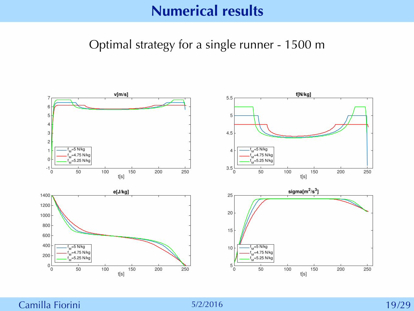
Optimal strategy for a single runner - 1500 m
19
Camilla Fiorini 5/2/2016 /29
Numerical results
[J/kg]
[N/kg]
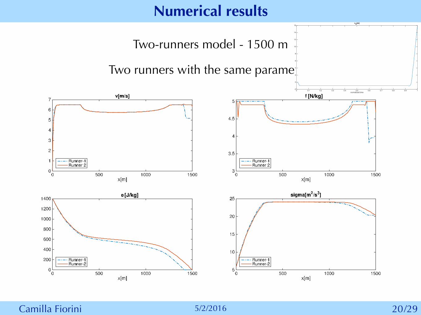
Two-runners model - 1500 m
Two runners with the same parameters
normalized time0 0.1 0.2 0.3 0.4 0.5 0.6 0.7 0.8 0.9 1
-2
0
2
4
6
8
10
12
14
16
xD
[m]
20

Camilla Fiorini 5/2/2016 /29
Numerical results
[J/kg]
[N/kg]
Two-runners model - 1500 m
The weaker can win starting behind
normalized time0 0.1 0.2 0.3 0.4 0.5 0.6 0.7 0.8 0.9 1
-1.5
-1
-0.5
0
0.5
1
1.5
2
xD
[m]
21

Camilla Fiorini 5/2/2016 /29
Numerical results
Two-runners model - 1500 m
The stronger starts behind
x[m]0 500 1000 15000
1
2
3
4
5
6
7v[m/s]
Runner-1Runner-2
x[m]0 500 1000 15003
3.5
4
4.5
5f
Runner-1Runner-2
x[m]0 500 1000 15000
200
400
600
800
1000
1200
1400e
Runner-1Runner-2
x[m]0 500 1000 15005
10
15
20
25sigma[m2/s3]
Runner-1Runner-2
[J/kg]
[N/kg]normalized time
0 0.1 0.2 0.3 0.4 0.5 0.6 0.7 0.8 0.9 1-5
0
5
10
15
20
25
30
35
40
45
xD
[m]
22
Camilla Fiorini 5/2/2016 /29
Numerical results
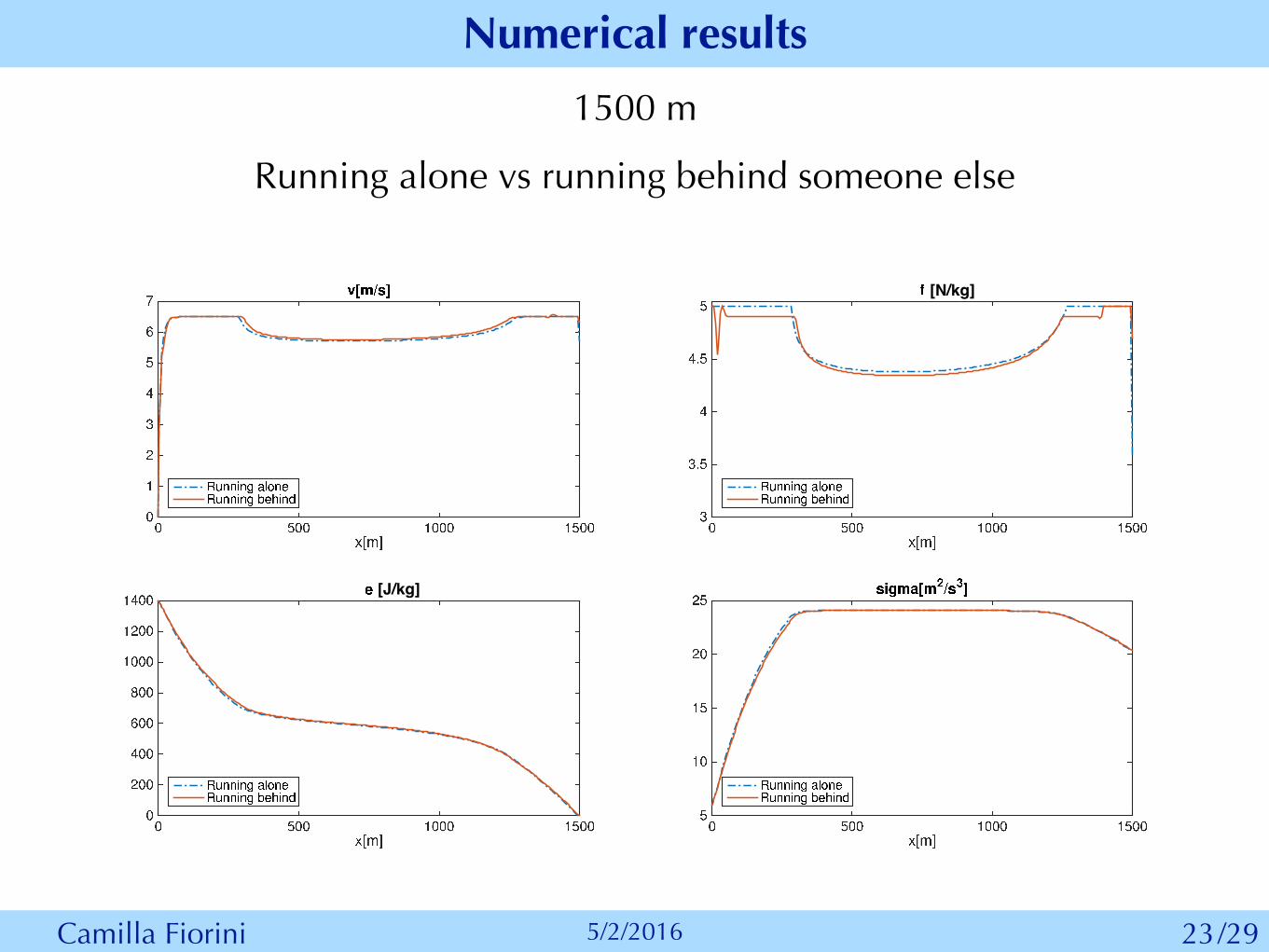
Running alone vs running behind someone else
[J/kg]
[N/kg]
1500 m
23

Camilla Fiorini 5/2/2016 /29
Numerical results
0 500 1000 1500x[m]
0
1
2
3
4
5
6
7
8
v[m
/s]
bending partsmodel real trackmodel straight
Real track model vs straight line model
1500 m
24

Camilla Fiorini 5/2/2016 /29
Numerical results
Parameter identification
lane 1
lane 3
lane 6
40m
32.69m
21.66m
Six runners
Three paths
D = 180m
Time splits every 10m
25
Camilla Fiorini 5/2/2016 /29
Parameter identification
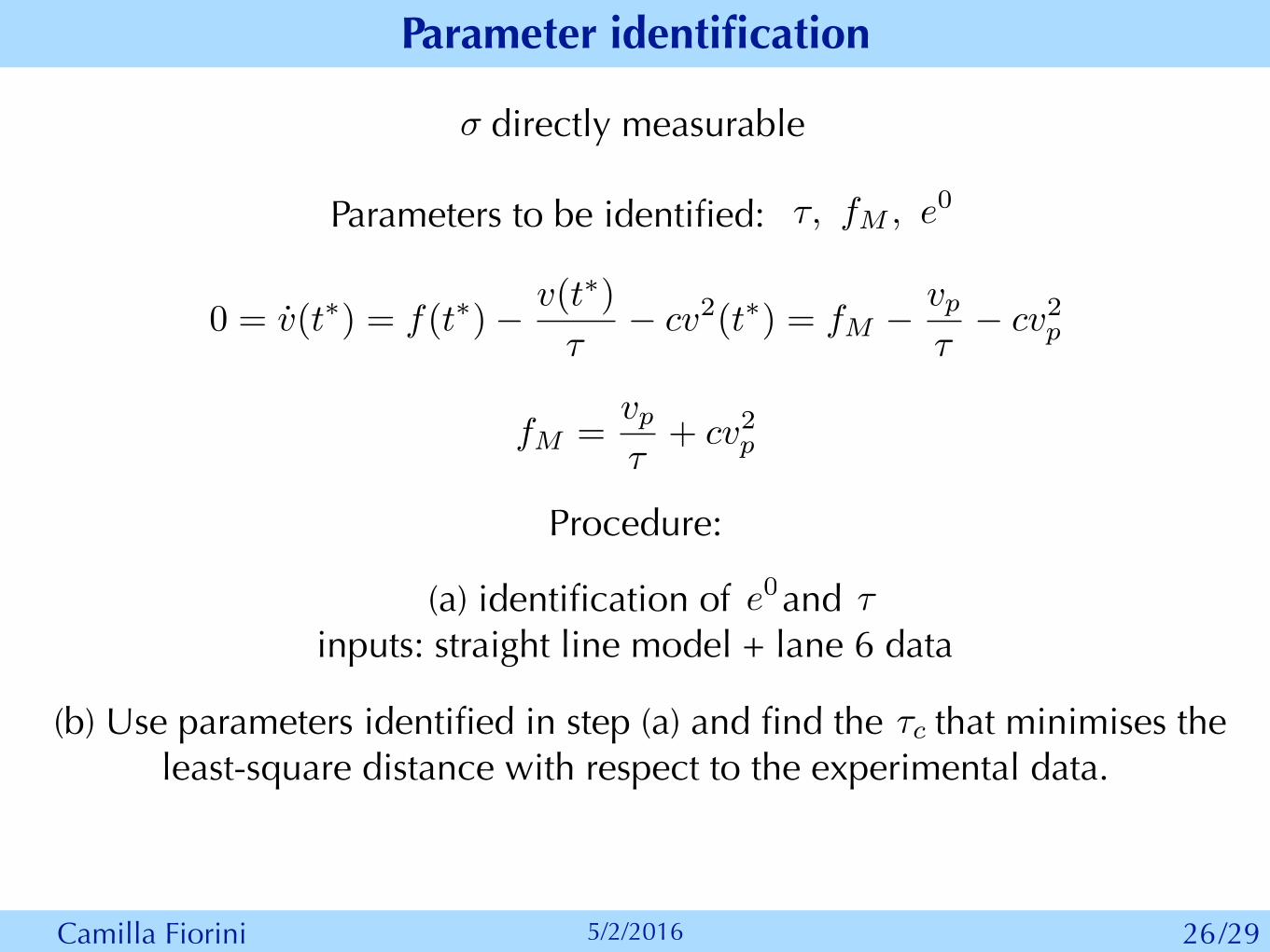
directly measurable
Parameters to be identified:
�
⌧, fM , e0
0 = v(t⇤) = f(t⇤)� v(t⇤)
⌧� cv2(t⇤) = fM � vp
⌧� cv2p
(a) identification of and inputs: straight line model + lane 6 data
(b) Use parameters identified in step (a) and find the that minimises the least-square distance with respect to the experimental data.
Procedure:
e0 ⌧
⌧c
fM =vp⌧
+ cv2p
26

Camilla Fiorini 5/2/2016 /29
Numerical results
Parameter identification
0 20 40 60 80 100 120 140 160 180x[m]
0
1
2
3
4
5
6
7
8
9
10
v[m
/s]
Gatien C1, tau1 = 0.2
Real trackStraight pathExperimental valuesBending parts
27

Camilla Fiorini 5/2/2016 /29
Numerical results
Parameter identification
0 20 40 60 80 100 120 140 160 180x[m]
0
1
2
3
4
5
6
7
8
9
10
v[m
/s]
Gatien C3, tau1 = 0.2
Real trackStraight pathExperimental valuesBending parts
28

Camilla Fiorini 5/2/2016 /29
Numerical results
Parameter identification
0 20 40 60 80 100 120 140 160 180x[m]
0
1
2
3
4
5
6
7
8
9
10
v[m
/s]
Gatien C6, tau1 = 0.2
Real trackStraight pathExperimental valuesBending parts
29

Thank you for your attention