optimal tax and benefit policies with multiple observables
TRANSCRIPT
Optimal Tax and Benefit Policies withMultiple Observables
Etienne Lehmann, Sander Renes, Kevin Spiritus and Floris Zoutman ∗
February 1, 2018
PRELIMINARY VERSION
This note was initially written individually by Kevin Spiritus. It is now a part of aproject with Etienne Lehmann, Sander Renes, and Floris Zoutman. It is intended to becombined with Renes and Zoutman: ”As Easy as ABC? Multi-dimensional Screeningin Public Finance” (2017) and Lehmann: ”Optimal multidimensional and nonlineartaxation” (2017).
We study the optimum for tax problems with multidimensional tax basesand multidimensional heterogeneity of agents. We use the Euler-Lagrangeformalism to show how the optimal tax function balances efficiency versusequity considerations. The equity considerations are captured in a localizeddistributional characteristic, a generalization of the distributional charac-teristic first introduced by Feldstein (1972a,b). We apply these findings tothe optimal joint taxation of couples, and to the optimal mixed taxation ofcapital and labour income. We show robustness for pooling, bunching andrestrictions to the tax base.
Keywords: optimal mixed taxation, heterogeneous agentsJEL Classification: H21, H23, H24
1. IntroductionThe problem of optimal mixed taxation with multidimensional types, as stated by Mir-rlees (1976), has long eluded an exact solution. Most optimal-tax models taking intoaccount distributional concerns, in the tradition of Mirrlees (1971) and Atkinson and∗Lehmann: CRED (TEPP) University Pantheon-Assas Paris 2; Renes: Erasmus School of Economics at
University Rotterdam; Zoutman: NHH Norwegian School of Economics; Spiritus: Erasmus UniversityRotterdam, KU Leuven and Tinbergen Institute.
1

Stiglitz (1976), assume that a single parameter, often an ability parameter, drives dif-ferences between agents. This makes it difficult to study problems with multiple taxbases where more extensive type heterogeneity is deemed relevant. The literature offersno exact solution for example for the optimal mixed tax problem for labour and capitalincome when individuals differ simultaneously in a number of dimensions, e.g. in theirabilities and their preferences for labour supply and for investment, or in the inheritancesthey receive. Atkinson and Stiglitz (2015, p.xxi) list this question as one of the centralcurrent challenges in public finance. My aim in this paper is to provide a solution.
This paper makes two contributions. The first is that it is the first to characterizethe full optimum in terms of sufficient statistics and distributional characteristics. Thesecond is that it introduces a solution method which avoids the labour intensity andtechnical complications inherent to existing approaches. I apply my results to a numberof previously unsolved problems.
In optimal-tax theory it is customary to search for a tax system that maximizes a so-cial welfare function. It maps the “social state”, e.g. the distribution of attained utilitylevels or disposable incomes, on a scalar indicating a social judgment about that socialstate. It takes into account normative criteria, for example social preferences for redis-tribution, efficiency and responsibility. The maximization of the social welfare functionoccurs subject to constraints such as the government budget, incentive compatibility andrestrictions to tax and benefit policies. Boadway (2012) gives an overview of the recentliterature.
The case with a one-dimensional tax base has been well studied. Saez (2001) andJacquet and Lehmann (2016) offer exact solutions. The optimal tax rate at each incomelevel is formulated as a product of three terms, traditionally denoted as A, B andC,1 where the A-term relates negatively to the excess burden associated with the tax,the B-term concerns the distributional advantage of levying an additional tax from allindividuals at higher income levels, and the C-term takes into account the thickness ofthe income distribution at higher levels.2
There are two broad approaches in the literature to study the problem with multidi-mensional tax bases, both of which lead to technical complications. The dual approachto optimal taxation, which directly uses the tax function as an instrument, is gainingpopularity (see e.g. Christiansen (1984), Saez (2002), Werquin, Tsyvinski, and Golosov(2015)). It is customary to first construct perturbations of the tax function, and then tofind conditions for such perturbations to have zero effect on social welfare. Some authorsconstruct combined perturbations such that the total effect on the government budgetis zero (e.g. Christiansen (1984), Saez (2002)). Others use Gateaux derivatives in thedirection of some reform function (Werquin, Tsyvinski, and Golosov (2015)). Althoughthe perturbation approach yields important insights, it becomes cumbersome when morecomplex tax systems are studied.
Saez (2002), one of the founders of the perturbation approach, makes an important1See for example Diamond (1998, p.86) for an early use of this notation.2Gerritsen (2016) and Scheuer and Werning (2016) use perturbations to study the problem with a
one-dimensional tax base from different angles.
2

advancement by finding conditions for optimal commodity taxes to be non-uniform. Hismodel is robust for multidimensional heterogeneity of the agents. He leaves findingoptimal tax formulas as an “extremely useful” and “important task” for future research(2002, p.229). Werquin, Tsyvinski, and Golosov (2015) go beyond desirability conditions,finding a second-order partial differential equation for the tax function, characterizingthe optimum for a quite general multidimensional problem. They stop short of solvingthis equation.
The second, more traditional approach to study the optimal-tax problem is referred toas the primal or the mechanism design approach. Instead of using variations to the taxfunctions to figure out the optimum, one looks for an optimal allocation using individualdecision variables as controls, for example the consumption and labour supply variablesof the different individuals. The social welfare function is optimized using a Hamiltonianor a Lagrangian. This leads to optimality conditions for the tax wedges in a fairlystraightforward way. The greater challenge is to find a tax function which implementsthe optimum. An optimal tax system will generally be prohibitively complicated. Ina setting with multiple periods, for example, tax liabilities will generally depend innon-separable ways on labour income and capital incomes in all periods at the sametime. Often it appears impossible to characterize this function analytically. Even incases where an analytical solution can be found, the task of reformulating it in termsof observable statistics can be labour intensive. A further limitation of the approach isthat it has difficulties to handle multiple dimensions of heterogeneity of the agents, orimportant restrictions to the tax function.
Diamond and Spinnewijn (2011) use this mechanism design approach to study theproblem of optimal mixed taxation of capital and labour income with heterogeneousabilities and discount rates. They find desirability conditions in terms of the fundamen-tals of the model. They do not characterize the optimum.
Mirrlees (1976) states the full optimization problem with a multidimensional tax baseand multidimensional heterogeneity of the agents, but solves it only for the case withone-dimensional heterogeneity of the agents. For the case with multidimensional het-erogeneity he finds a second-order partial differential equation for the utility profile asa necessary condition for the optimum. Kleven, Kreiner, and Saez (2007) study theoptimal joint taxation of couples, finding a necessary condition of the exact same form.
Interestingly, the second-order partial differential equation found by Mirrlees (1976)has the same form as the previously mentioned equation found by Werquin, Tsyvinski,and Golosov (2015) – though it is expressed in terms of fundamentals of the model ratherthan in terms of observable variables. Since second-order partial differential equationsof similar form are encountered in both approaches, the key to solving the optimal-taxproblem appears to lie in finding solutions for these equations.
Renes and Zoutman (2016a) make important headway by treating the second-orderdifferential equation found by Mirrlees (1976) as a first-order differential equation in themultipliers of the incentive compatibility constraint. They show that these multipliersform a conservative vector field, and use this fact to convert the problem into a newsecond-order partial differential equation for which solution methods are more readilyavailable. They apply the Green functions approach, well-studied in physics and en-
3
gineering but less familiar in economics, to characterize the optimum. Their methodstill has a number of limitations. It cannot handle the case with more types than taxbases – e.g. the cases treated by Saez (2001, 2002) and Jacquet and Lehmann (2016).It also requires perfect screening, meaning that at most one type pools at each tax-baselevel. The solutions are formulated in terms of fundamentals of the problem ratherthan observable variables, lacking a straightforward economic interpretation. And theprocedure to convert the problem to a new second-order partial differential equation iscomplicated.
The present paper suggests an alternative. The central methodological insight isthat the problem of optimal multidimensional taxation is essentially a field-theoreticalproblem: the tax function is a scalar field over the tax base space, which is shaped inorder to optimize an objective, a social welfare functional subject to a resource constraint.Both the level of the tax function at each value of the tax base (the tax liability) as itsgradient (the marginal tax rates) have an impact and need to be taken into account.
A central difference with traditional field theory is that the objective function is notdefined over the tax base space, but over a set of individuals, members of a multidimen-sional type space. These individuals are free to choose any value in the tax base space,as long as they can afford it. It is even possible for multiple types to choose the samevalue of the tax base. This difference leads to a number of complications, but theseare not insurmountable. With some modifications it is still possible to characterize theoptimal tax function using well-established techniques.
I show how this optimum is characterized by an Euler-Lagrange equation, first graphi-cally and then formally. This is a second-order partial differential equation which gener-alizes the equation found by Werquin, Tsyvinski, and Golosov (2015). Next I show howstandard methods can be used to characterize solutions to the Euler-Lagrange equation.I treat it as a first-order partial differential equation, and introduce multidimensionalGreen functions to characterize the optimum directly in terms of observable quantitiessuch as population densities, average behavioural responses and average welfare weightsat each value of the tax base.
An advantage of using the tax function as an instrument, rather than the allocation,is that it immediately leads to a characterization in terms of sufficient statistics, similarto the findings of Saez (2001) for a one-dimensional tax base. This makes the resultsmuch easier to interpret. Using the tax function as an instrument also makes that noincentive compatibility constraints need to be taken into account, avoiding the usualimplementation issues that surface in multidimensional problems. Moreover, it allowsto remain agnostic about the process determining individual behaviour, as I do in mostof the paper, and it allows to distinguish between the wellbeing measures taken intoaccount by the planner on one hand, and the preferences driving individual behaviouron the other.
The resulting characterization of the optimum is very similar to that for the problemwith linear taxes as stated by Atkinson and Stiglitz (1980, p.386-390). At any givenvalue of the multidimensional tax base, the efficiency effects of a marginal tax reformshould be balanced against its distributional effects. The proportional reduction of anycomponent of aggregate demand, along compensated demand curves, should be equal
4
to a local distributional characteristic of that component. The distributional side ofthis equation is new. It is a localized version of the distributional characteristic firstintroduced by Feldstein (1972a,b). If we associate a marginal social welfare weight witheach potential value of the tax base, then the local covariance of these welfare weightswith the tax-base component under consideration determines the distributional impacton social welfare. These findings apply even when the dimensionality of the type spaceis higher than that of the tax base space.
Although these are interesting insights, they still do not teach us much about theunderlying economics. I go on to repeat the same techniques in the type space, stillusing the tax function as an instrument. This again leads to a characterization of theoptimum where efficiency effects of a tax reform are balanced against equity effects.The equity effects now consist of two parts. First there are again local distributionalcharacteristics of the different traits of the individuals. If for example individuals whoreceive a larger inheritance have much lower marginal social welfare weights, this willlead to a large distributional characteristic for this trait. Second, there are additionalterms indicating how well a given component of the tax base is suited to target a giventrait of the individuals. These two elements, how much we care about particular traits(a normative part) and how well these traits can be targeted (an informational part),determine the distributional impact of a given tax base component. These results extendfindings by Mirrlees (1976) and Renes and Zoutman (2016a).
I illustrate my results using a number of examples, applying either to the joint taxationof couples or to the joint taxation of labour and capital incomes. My aim is not togive a thorough discussion of these topics. Indeed, important normative issues such aswhether the government should tax individuals or families, or how families should enterin social preferences, are not taken into account. Neither do I discuss what social welfareweights should look like, e.g. whether the government should support couples where oneindividual stays at home, or rather whether it should stimulate equal participation inthe labour market. The point I want to illustrate is that once the tax base, the socialobjective and a behavioural model have been chosen, then the techniques in this papercan be used to gain insight into the optimal tax system.
Still these examples yield some interesting results. For the problem of the optimaljoint taxation of couples, as posed by Kleven, Kreiner, and Saez (2007), I am able tocharacterize for the first time the solution in terms of local distributional characteristicsof the households. For the optimal tax mix between capital income and labour income,I study the case where discount rates are heterogeneous, a case that is excluded e.g.by Werquin, Tsyvinski, and Golosov (2015). I confirm a number of classical reasonsfor marginal tax rates on capital income to be non-zero: when discount rates are di-rectly driven by labour abilities (Saez, 2002), when labour supply is a complement or asubstitute to consumption (Corlett and Hague, 1953), and when investment technologyis affected by an ability parameter. The latter complements the findings of (Gerritsenet al., 2015). Even when neither of these reasons applies, an accidental correlation be-tween the labour abilities and the discount rates suffices for the optimal marginal taxrate on capital income to be non-negative (Diamond and Spinnewijn, 2011). I show thatthe latter correlation remains sufficient even when social welfare weights are constructed
5

such that they do not depend on the discount rates, holding individuals responsible fortheir preferences. I show that when rates of returns depend on the individuals’ discountrates, then the optimal marginal tax rates on capital income again differ from zero. Istate for the first time the optimality condition, extending on the desirability conditionsformulated in the past literature. It is straightforward to extend this formulation e.g. toheterogeneous wealth endowments.
There are a number of possible complications while dealing with multidimensionaltax bases and multidimensional heterogeneity of the agents. The most important is thepossibility of bunching. Although Kleven, Kreiner, and Saez (2007) show that bunchingmay not be a problem for a large range of social welfare objectives, it cannot simplybe ignored. I do not attempt to characterize when and where bunching will occur inthe optimum. I rather give necessary conditions to check whether a given tax function,with our without bunching, is optimal given information about population densities andbehavioural responses. I show that the approach described in this paper remains valideven when bunching occurs. Similarly, I show how to deal with potential issues such aspooling, double deviations, and restrictions to the tax base space.
To the best of my knowledge, the possible use of the Euler-Lagrange formalism ismentioned just once in the optimal-tax literature. Bohacek and Kejak (2016) constructan Euler-Lagrangian to solve a dynamic problem with heterogeneous types and a one-dimensional tax base. They prove the correctness of the approach for their specificproblem. They provide an analytical solution only for the end-points, resorting to sim-ulations for the rest of the type distribution. The above-mentioned partial differentialequation identified by Werquin, Tsyvinski, and Golosov (2015) is a specialized versionof the Euler-Lagrange equation. It was derived for a specific optimal tax problem, andexcludes for example heterogeneous discount rates.
The present paper shows the general applicability of the Euler-Lagrange framework,so that it is no longer necessary to construct new perturbations and list their effectseach time a new problem is encountered. Furthermore, as far as I know, it is the first toidentify the localized distributional characteristics that characterize the optimum.
In this paper I do not address the optimal choice of the tax base. I take a tax baseas given, and I determine the optimal tax function over this base. Since the problemis not so difficult to solve with a separable tax function (see e.g. Kleven, Kreiner, andSaez (2007)), I consider non-separable tax bases only – although I will encounter anexample where the optimal tax system turns out to be separable. The methods inthis paper remain valid even when the tax system is incomplete, e.g. in the cases oftax avoidance or income shifting as studied by Christiansen and Tuomala (2008). Theapproach also allows solving more general problems, e.g. with a government aimingto gain sufficient votes to remain in power, or a formulation incorporating alternativenormative convictions, e.g. using generalized Pareto weights as discussed for a one-dimensional tax base by Saez and Stantcheva (2016).
I start in section 2 by introducing the model and identifying the behavioural responsesto tax reforms. I introduce the Euler-Lagrange formalism in section 3. I show intuitivelyand formally how the Euler-Lagrange equation is a necessary condition for the optimum.In section 4 I then use the Euler-Lagrange equation to find a more intuitive characteri-
6

zation of the optimum, using sufficient statistics in the tax base space, and in section 5 Ireformulate this characterization in terms of economic fundamentals. Finally in section6, I list a number of potential complications, and I show how they can be overcome.
2. ModelWe study a population of individuals who are distinguished by a K-dimensional columnvector of characteristics θ ≡
(θ1, . . . , θK
)ᵀ, with superscript .ᵀ denoting a transpose.
This vector is also called the type of the individual. The set of all such vectors is denotedΘ, which is a convex subset of the real vector space RK . The type of an individual caninclude characteristics such as ability, gender or preferences. The types have a cumulativedistribution function FΘ (θ), with corresponding density function fΘ (θ).
There is a government which does not observe the type of the individuals, but it doesobserve for each individual an L-dimensional column vector x ≡
(x1, . . . , xL
)ᵀwhich is
called the tax base. The values of the tax base are elements of the tax base space X ,which is a convex subset of the real vector space RL. I denote the cumulative distributionfunction as FX (x), with corresponding density function fX (x). The government usesthe value x of the tax base for each individual to determine their tax liability T (x),which is a scalar-valued, potentially nonlinear function.
Each individual makes a number of decisions, given the tax function and his type.These decisions may include for example labour supply, consumption of different goods,savings, and so on. They may also include reporting decisions such as how much taxes toevade, or how much labour income to declare as capital income. The government does notobserve all of these decisions. Together with the type, these decisions do determine thetax base, which is observed by the government. For example, although the governmentmay not observe an individual’s labour effort and his ability, it does observe the grosslabour income declared by the individual. To facilitate my exposition, I will act as if theindividual chooses the value of his tax base directly, given his type and the tax function.This leads to the vector-valued tax base function x (θ, T ).
The government chooses the function T in order to maximize social welfare, which isthe sum of individual wellbeing measures v (θ, T ):
maxT
∫Θv (θ, T ) dFΘ (θ) . (1)
The individual wellbeing measure is determined by the individual type and by the taxfunction. It may simply be defined as the indirect utility of an individual, or as someother measure of individual wellbeing, taking into account social normative judgments.There is not necessarily a direct link between the wellbeing measure taken into accountby the government, and individual behaviour.
The government aims to levy an exogenously determined revenue, which without lossof generality is normalized to zero. This leads to the government budget constraint:∫
ΘT (x (θ, T )) dFΘ (θ) = 0. (2)
7
The simultaneity in this formulation requires careful attention. The government budgetconstraint depends on the tax liability owed by each individual, while the chosen values ofthe tax base by the individuals depend again on the tax function. One should distinguishconceptually between the function T , and its value T (x) at a particular value of the taxbase.
Denote the partial derivatives of the tax function using a subscript: Tl ≡ ∂T/∂xl, anddenote the gradient of the tax function as follows:
∇xT (x) ≡ (T1 (x) , . . . , TL (x)) . (3)
I will refer to it in short as the tax gradient.To find necessary conditions for a tax function T to be optimal, I use the fact that a
small tax reform should leave social welfare unchanged. I assume that for an individualwho chooses value x (θ, T ) of the tax base, his response to a small tax reform will be willbe along the intensive margin, excluding discrete jumps.3 I assume that his response willbe determined only by the change in the tax liability at x, and by the change in the taxgradient at x. Locally, individual behaviour thus remains unchanged if the tax functionis replaced by a linearized version, since this leaves the tax liability and the tax gradientunchanged. For example in the neoclassical labour supply model, where an individualchooses his labour supply such that the indifference curve at his chosen bundle is tangentto his budget set, the individual would not change his behaviour if the budget set werelinearized.4 Furthermore, I assume that individual wellbeing is affected only by a changein the tax liability, and not by a change in the gradient or higher-order derivatives ofthe tax function. If the chosen wellbeing measure is the indirect utility function, thenthis assumption is automatically fulfilled because of the envelope property.
I use a subscript T to denote the effect of a local change in the tax liability. Forexample, xT (θ, T ) denotes the column vector containing the effects of a change in thetax liability on the different components of the tax base chosen by a type-θ individualin presence of tax function T :
xT (θ, T ) ≡
x1T (θ, T )
...xLT (θ, T )
.Similarly, the marginal social value of an extra unit of income for a type-θ individualequals −vT (θ, T ).
I use a subscript Tl to denote the effect of a local change in the l-th component of thetax gradient, holding constant the tax liability at the original value of the tax base. The
3More precisely, I assume that the impact of discrete jumps on social welfare is of second order, andthat it can be ignored when studying marginal tax reforms. This excludes the empirically relevantcases where individuals face discrete choice sets, or where they do not re-optimize continuously.
4This assumption is not innocuous. For example in presence of uncertainty, the local curvature of thetax function will affect the variance of after-tax income, which will affect individual behaviour. Thederivations in this paper can be extended to include higher-order derivatives of the tax function,analogous to the methods used in the calculus of variations with higher-order derivatives. For anoverview, see for example Courant and Hilbert (1953, p.190).
8

effects of a change in the tax gradient on the tax base chosen by a type-θ individual aresummarized in the following matrix:
x∇T (θ, T ) ≡
x1T1
(θ, T ) · · · x1TL
(θ, T )... . . . ...
xLT1(θ, T ) · · · xLTL
(θ, T )
. (4)
Note that even if I assume that small local reforms to the curvature of the tax functiondo not affect the chosen values of the tax base, the responses to a marginal reform ofthe tax liability or the tax gradient are affected by the curvature. The reason is thatwhen the tax function is nonlinear, the response of the value of the tax base to a reformtriggers an additional change in the gradient of the tax function, which causes second-round behavioural effects.5
3. Euler-Lagrange FormalismThe problem facing the government is to maximize social welfare (1), subject to gov-ernment budget constraint (2), using the tax function T as an instrument. A necessarycondition for the function T to be optimal, is that a marginal tax reform leaves socialwelfare unchanged.
Any tax reform triggers a number of effects. There is an impact on individual well-being, and as such a direct effect on social welfare. There is also a mechanical effecton government revenue, controlling for changes in individual behaviour, and there areadditional effects on government revenue, attributable to the changes in individual be-haviour. Requiring that these effects sum to zero then yields a necessary condition forthe optimum.
A difficulty is that it is impossible to study all admissible reforms and to list theireffects. Luckily we can use the fundamental lemma of the calculus of variations, whichstates that it suffices to study every extremely local reform to the tax function, changingthe liability at one particular value of the tax base and taking into account the inducedchanges in the tax gradient around it.
In the present section I will construct such local tax reforms, and show intuitively howthey lead to a partial differential equation, a necessary condition for the optimum, whichis similar to the Euler-Lagrange equation often used in the calculus of variations. I willfirst show in subsection 3.1 how for one-dimensional tax bases, this equation correspondsto the ABC-style optimal-tax equation that is found in the literature. Next I will arguehow it is straightforward to construct similar local tax reforms for multidimensionalbases, and I show how a similar Euler-Lagrange equation characterizes the optimum. Insubsection 3.2 I do this graphically for a two-dimensional tax base, and in subsection 3.3I formally prove the multidimensional optimal-tax condition. I will treat the boundaryconditions for the optimum in subsection 3.4.
5These additional effects are similar to those discussed by Jacquet and Lehmann (2016), and are incontrast with the linearized counterparts in Saez (2001).
9

I exclude for now the possibility of bunching. Bunching occurs when there is a masspoint, and thus a discontinuity, in the population density fX in the tax base space. Thissituation could occur e.g. at an edge of the tax base space, because a range of types endsup in a corner solution, or as Ebert (1992) illustrates it could also occur in the interiorof the tax base space, leading to a kink in the optimal tax function. I will treat thispossibility in section 6. Throughout the present section I assume that the tax functionand the objective function are sufficiently smooth, excluding the possibility of kinks orbunching.
Note that I follow Jacquet and Lehmann (2016) in distinguishing between bunchingand pooling: the latter situation occurs when different types choose the same value ofthe tax space without forming a mass point. This situation occurs for example whenthe dimension of the type space is higher than the dimension of the tax base space.Throughout this section I allow for any number of dimensions in the type space, andthus for pooling.
3.1. One-Dimensional Tax BaseThe case with a one-dimensional tax base is well understood. It was first solved forone-dimensional types by Mirrlees (1971). Its intuition for multidimensional types isdiscussed by Saez (2001), and formalized by Jacquet and Lehmann (2016). I will treatit here in a different way, that can be extended more readily to the case of a multidi-mensional tax base.
To focus our thoughts, I will treat the case of an optimal labour income tax. I denotegross labour income as z, the corresponding tax liability is T (z) and the correspondingmarginal tax rate is Tz (z). I denote the cumulative distribution function of gross labourincome as FX (z), with corresponding density function fX (z). I denote the supportof the latter function as [z, z]. Saez (2001) finds the optimal marginal tax rate at anarbitrary gross income level Z by increasing the marginal tax rate by a small quantitydTz over an interval of small width dZ, as illustrated in figure 1. Individuals at incomelevel Z experience an increase in their marginal tax rate, which leads to compensatedeffects, and individuals at higher income levels experience an increase in their tax liability,which leads to income effects. Saez (2001) adds together all mechanical, behavioural andwelfare effects of this reform, and requires that the total effect on social welfare shouldbe zero. This, together with a transversality condition, leads directly to a necessarycondition for the tax optimum.
The difficulty for us is that it is not clear how to extend this reform to the case with amultidimensional tax base. I will introduce a different kind of reform which leads to thesame characterization of the optimum as the one found by Saez (2001), but which canbe readily extended to higher dimensions. The trick lies in still performing the reformintroduced by Saez (2001), namely increasing the marginal tax rate at gross income Zby a quantity dTz over an interval of width dZ, and adding a reverse reform at a smalldistance δ � dZ. In other words, at gross income Z + δ, there is a decrease in themarginal tax rate by the same quantity dTz over an interval of the same width dZ. Theresulting tax reform is shown in figure 2.
10

Figure 1: The tax reform as introduced by Saez (2001). At gross income level Z, overan income range of width dZ, the marginal tax rate is increased by dTz. Atincome levels above Z, the tax liability is increased by dZdTz.
(a) The original tax function and the reformed tax function.
Z z
T (z)
dZ
dTz
dZdTz
(b) The size of the tax reform.
Z zdZ
dTz
dT (z)
dZdTz
11

Figure 2: The tax reform for a one-dimensional tax base as introduced in this paper.The tax reform introduced by Saez (2001) is maintained at gross income levelZ, but it is reversed at gross income level Z + δ, with δ � dZ small.
(a) The original tax function and the reformed tax function.
Z z
T (z)
dZ
dTz
dZdTz
dZ
−dTz
Z + δ
(b) The size of the tax reform.
Z zdZ
dTz
dT (z)
dZdTz
Z + δdZ
δ
−dTz
12

The social-welfare effect of this marginal reform should of course be zero in the op-timum, as is the case for any marginal reform. A reason for choosing this particularreform, is that any broader reform could be decomposed into smaller reforms of the kindintroduced here. This intuition is captured more formally in the fundamental lemma ofthe calculus of variations, which I will apply in subsection 3.3.
This reform has a number of effects. First, there are behavioural effects at Z, whereindividuals experience an increase dTz in their marginal tax rate. The number of in-dividuals experiencing this change equals fX (Z) dZ. A difficulty is that individuals ofdifferent types might pool at the same gross income level Z. Denote the average responseof all individuals pooling at Z to a reform of the marginal tax rate as zTz (Z).6 The totalresulting change in government revenue will then be
[zTzTzf
X ] (Z) dTzdZ.7 Second, andsimilarly, the decrease in the marginal tax rate at Z+ δ causes a decrease in governmentrevenue by
[zTzTzf
X ] (Z + δ) dTzdZ. Third, individuals on the interval [Z,Z + δ] expe-rience an increase of their tax liability by dTzdZ. This leads to a mechanical effect ontax revenue equal to dTzdZ
∫ Z+δZ fX (z) dz . Fourth, this increased tax liability leads to
welfare effects, which equal dTzdZ∫ Z+δZ (vT (z) /λ) fX (z) dz, where λ is the government
budget multiplier which converts the individual wellbeing measure to monetary units.Fifth, the increased tax liability also leads to behavioural effects, which have revenueeffect dTzdZ
∫ Z+δZ
[zTTzf
X ] (z) dz. Note that we do not need to account for the changein the density function fX (z): since we multiply the average per-individual effect withthe number of individuals experiencing the reform, we need to work with the originaldistribution before the reform takes place.8
A necessary condition for the tax function T to be optimal, is that the above reformdoes not affect social welfare. Adding all effects, dropping the common factor dTzdZ,dividing by δ, and requiring that the terms sum to zero leads to the following condition:
1δ
∫ Z+δ
Z(1− α (z)) fX (z) dz =
[zTzTzf
X ] (Z + δ)−[zTzTzf
X ] (Z)δ
, (5)
where α (z) ≡ − [vT /λ+ zTTz] (z) denotes the average net marginal effect on socialwelfare, in monetary units, of an exogenous income increase for individuals at incomelevel z, as first introduced by Diamond (1975). This equation tells us that the social-welfare effect of a change in the tax liability at a small interval [Z,Z + δ] in the incomedistribution, should be compensated by the effects of the ensuing changes in the taxgradient around this interval.
If we now take the limit for very small values of δ, keeping dz � δ, we are studying theeffect of an extremely local reform to the tax function. The left-hand side of equation(5) will converge to (1− α (Z)) fX (Z), while the right-hand side by definition converges
6Throughout this paper, for any function g : Θ → RD, with D some dimensionality, I will denote usinga bar g (x) the average of the function g for all individuals pooling at tax base x.
7Where necessary, I will denote the product of the values of any functions g (x) and h (x) as [gh] (x).8I ignore the impact of individuals making a discrete jump due to the reform, e.g. because they were
almost indifferent between two bundles before the reform. It is of second order compared to the totalimpact.
13

to the derivative of zTzTzfX with respect to z at Z:
(1− α (Z)) fX (Z) = d
dz
[zTzTzf
X]
(Z) . (6)
This differential equation is similar to the one-dimensional Euler-Lagrange equationfound in the calculus of variations. The main difference is that the objective of our opti-mization is defined as an integral over the type space, while the tax instrument is definedin the tax base space. In the traditional version of the Euler-Lagrange equation, boththe objective and the instrument would be defined in the same vector space. Averagingthough at each value of the tax base takes care of this difference. In subsection 3.3 Iderive this equation more rigorously.
Since I exclude for now the possibility of bunching, the marginal tax rates should bezero at the edges of the tax base space:
Tz (z) = Tz (z) = 0.
There is no point in distorting labour supply at the lowest income level, as there are noindividuals at lower income levels to whom the proceeds can be redistributed. Similarly,there is no point distorting labour supply at the highest income level, as there is nobodyat higher income levels to levy additional taxes from. This point was first made for thetop by Sadka (1976), and for the bottom by Seade (1977).9
Integrating (6) and using the latter boundary conditions leads to the necessary optimal-tax condition:
∀z :∫ z
z
(1− α
(z′))fX
(z′)
dz′ = −zTz (z)Tz (z) fX (z) , (7)
with transversality condition: ∫ z
zα(z′)fX
(z′)
dz′ = 1.
The transversality condition conforms to the notion, discussed by Jacobs (2013), thatthe marginal cost of public funds equals one when the tax system is optimal.
By performing this integration, the local reform that I constructed at one specific valueof the tax base, is repeated over the interval [z, z], recovering the tax reform constructedby Saez (2001). Defining the elasticity e (z) ≡ −zTz (z) (1− Tz (z)) /z, holding constantthe tax liability T (z) at z, we can reformulate this in a more traditional ABC-form:
∀z : Tz (z)1− Tz (z) = A (z)B (z)C (z) , (8)
9I will derive these boundary conditions more formally for the formalism of this paper in subsection3.3.
14

with:
A (z) ≡ 1e (z) ,
B (z) ≡∫∞z (1− α (z′)) fX (z′) dz′
1− FX (z) ,
C (z) ≡ 1− FX (z)zfX (z) .
The A-term contains the inverse of the average elasticity of gross income with respect tolocal changes in the marginal tax rate, keeping constant the tax liability at income levelz. The B-term contains the average redistributional effect of taking one euro from eachindividual above income level z and lowering the tax liability elsewhere in the incomedistribution. The C-term is a hazard rate, which relates the number of individuals whoare at the income level where the reform to the marginal tax rate takes place – whoselabour supply decisions are being distorted, to the number of individuals who are athigher income levels – from whom additional funds are levied for redistribution.
3.2. Two-Dimensional Tax BaseThe tax reform which I introduced for a one-dimensional tax base in the previous subsec-tion, can be extended to a two-dimensional tax base. Suppose the government observes atax base (z, y) for all individuals. Its components z and y could be thought of for exam-ple as labour income and capital income, or the incomes of two individuals in a couple.The government aims to maximize social welfare by setting a joint, non-separable taxfunction T (z, y), taking into account the multidimensional heterogeneity of the agents.A necessary condition for the tax function to be optimal is that a small tax reform leavessocial welfare unchanged. To fix thoughts, I will refer to the tax base components aslabour income and capital income.
Consider a small rectangular area in the tax base space delineated by an interval[Z,Z + δZ
]in the labour income distribution, and an interval
[Y, Y + δY
]in the cap-
ital income distribution. I introduce a number of tax reforms within this rectangle[Z,Z + δZ
]×[Y, Y + δY
]. These reforms are illustrated in figure 3. Around labour in-
come Z, over an infinitesimal width dX, increase the marginal labour income tax by dTx.Conversely, decrease it by dTx over width dX around labour income Z + δZ . Similarly,increase the marginal capital income tax by the same quantity dTx over the same widthdX around capital income Y , and decrease it by dTx around capital income Y + δY .
There are again a number of effects from these reforms. Let us first consider theincrease in the marginal tax rate on labour income in the rectangle delineated by intervals[Z,Z + dX] and
[Y, Y + δY
]. Reasoning similar to that of the previous subsection shows
that for each level of capital income y within this rectangle, the total effect on thegovernment budget equals:
dTxdX[{zTzTz + yTzTy} fX
](Z, y) .
15

Figure 3: The tax reforms in two dimensions. At level Z of the first component of thetax base, over an income range of width dX, the marginal tax rate is increasedby dTx. At income level Z + δZ , with δZ � dX small, this reform is reversedby a decrease in the marginal tax rate by dTx over an income range of widthdX. Similar reforms are implemented for the second component of the taxbase. Within the rectangle at which the reforms take place, the tax liability isincreased by dTxdX.
(a) The tax base values where the reform takes place, form a small rectangle in the tax base space.
Z z
dX
dTx
−dTx
dX
Z + δZ
y
Y
dX
dX
Y + δY
−dTxdTx dT = dTxdX
(b) The size of the tax reforms.
Z
z
Z + δZ
y
Y
Y + δY
dT (z, y)
16

The total effect over the interval[Y, Y + δY
]follows by integrating the latter equation:
dTxdX∫ Y+δY
Y
[{zTzTz + yTzTy} fX
](Z, y) dy.
Similar effects occur at the other three edges of the rectangle on which the reforms takeplace.10
Within the edges of the rectangle the tax liability increases by dTxdX. Again followingreasoning similar to that of the previous subsection, we find the following effect on socialwelfare:
dTxdX∫ Z+δZ
Z
∫ Y+δY
Y(1− α (z, y)) fX (z, y) dydz,
with α (z, y) ≡ − [vT /λ+ zTTz + yTTy] (z, y) the average net marginal social welfareweight of individuals with labour income z and capital income y.
Setting the sum of all effects to zero, dividing by dTxdX and by δY δZ , and groupingsimilar terms on the same line yields:
1δY δZ
∫ Z+δZ
Z
∫ Y+δY
Y(1− α (z, y)) fX (z, y) dydz (9)
= 1δY
∫ Y+δY
Y
[{zTyTz + yTyTy
}fX] (Z + δZ , y
)−[{zTyTz + yTyTy
}fX](Z, y)
δZdy
+ 1δZ
∫ Z+δZ
Z
[{zTyTz + yTyTy
}fX] (z, Y + δY
)−[{zTyTz + yTyTy
}fX](z, Y )
δYdz.
The intuition here is similar to the one-dimensional case. The income effects of a localtax increase should be exactly cancelled out by the ensuing compensated effects in thesurrounding region.
Now take the limits δZ → 0 and δY → 0, keeping dX � δZ and dX � δY . Recognizeon the right-hand side the definition of partial derivatives with respect to z and y. Wecan rewrite:
(1− α (Z, Y )) fX (Z, Y ) = ∂
∂z
[{zTzTz + yTzTy} fX
](Z, Y )
+ d
dy
[{zTyTz + yTyTy
}fX]
(Z, Y ) .
Denoting the tax-base vector x ≡ (z, y) and writing X ≡ (Z, Y ), this can be shortenedin vector notation:
(1− α (X)) fX (X) =2∑l=1
∂
∂xl
[(∇xT · xTl
) fX]
(X) , (10)
10Note that with dX sufficiently small, the small inaccuracies in my exposition at the four corners ofthe square become negligible. A more formal prove is provided in the next subsection.
17

with gradient ∇xT introduced in equation (3), and the matrix containing behaviouralresponses xTl
in equation (4). This partial differential equation again is similar tothe Euler-Lagrange equation found in multidimensional variational analysis, with theadded complication that we need to average behavioural effects and welfare weights ateach income level. This partial differential equation is a necessary condition for the taxfunction T to be optimal. As in the one-dimensional case, it is amended with a boundarycondition for the gradient ∇xT (X), which I will discuss in subsection 3.4, and with thegovernment revenue constraint. Finding a fixed-point equation that characterizes theoptimum is not as straightforward as in the one-dimensional case, and is postponeduntil section 4.
Before doing this, we might gain some further intuition by integrating the Euler-Lagrange equation. Let V ⊆ X be a compact area in the tax base space, with apiecewise smooth boundary Γ (V ).11 Integrate Euler-Lagrange equation (10) over thisarea: ∫
V(1− α (x)) dFX (x) =
∫V
2∑l=1
∂
∂xl
[{∇xT (x) · xTl
(x)} fX (x)]
dx.
The left-hand side of this equation is the effect on social welfare of a unit increase inthe tax liability in the interior of the integration area V , as illustrated in figure 4a. Tointerpret the right-hand side, I rewrite it using a theorem from vector calculus, namedthe divergence theorem or Gauss’s theorem. For any point x at the boundary Γ (V ) ofour integration area, let x be an outward-pointing unit vector that is perpendicular tothe boundary, as illustrated in figure 4a. The divergence theorem then allows rewritingour integrated Euler-Lagrange equation:∫
V(1− α (x)) dFX (x) =
∫Γ (V )
[{∇xT · x∇T · x} fX
](x) dΓ . (11)
The right-hand side of this equation is a surface integral. The term within squarebrackets, which is a scalar, is integrated over the boundary Γ (V ).
Note in figure 4b that due to the increased tax liability in the interior of V , the taxgradient changes on the edge Γ (V ). The entity x∇T (x) · x is equal to the averagebehavioural effect caused by a unit change of the tax gradient that is perpendicular tothe boundary Γ (V ) at x. The term within curly brackets is the budgetary effect of thisbehavioural response for one individual at x, and the term fX (x) indicates how manyindividuals reside at that value of the tax base. The surface integral then adds theseeffects over the entire boundary Γ (V ). Equation (11) thus states that in the optimum,the effects caused by a unit increase in the tax liability at the interior of the area Vshould be exactly compensated by the behavioural effects due to the induced changes ofthe tax gradient at the edges of the area V .11I maintain this notation throughout this paper, also in higher dimensions: for any compact subset ofRL, let Γ (·) denote its boundary surface.
18
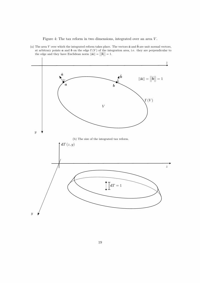
Figure 4: The tax reform in two dimensions, integrated over an area V .
(a) The area V over which the integrated reform takes place. The vectors a and b are unit normal vectors,at arbitrary points a and b on the edge Γ (V ) of the integration area, i.e. they are perpendicular tothe edge and they have Euclidean norm ||a|| =
∣∣∣∣b∣∣∣∣ = 1.
z
y
V
a
a
b
b
||a|| =∣∣∣∣∣∣b∣∣∣∣∣∣ = 1
Γ (V )
(b) The size of the integrated tax reform.
z
y
dT (z, y)
dT = 1
19

3.3. Higher-Dimensional Tax BasesIn the previous subsection I have shown that the reform that I have proposed for a one-dimensional tax base, can be readily extended to a two-dimensional tax base. I founda partial differential equation, the Euler-Lagrange equation, amended with boundaryconditions and the government budget constraint, to be a necessary condition for thetax optimum.
This reasoning can now be further extended to tax bases with an arbitrary numberof dimensions. The following theorem shows how Euler-Lagrange equation (10) can beextended to an L-dimensional tax base.12
Theorem 1. The tax optimum with an L-dimensional tax base with multidimensionalheterogeneity of the agents, in absence of bunching, complies to the following partialdifferential equation, referred to as the Euler-Lagrange condition:
∀x ∈ X : (1− α (x)) fX (x) =L∑l=1
∂
∂xl
[(∇xT · xTl
) fX]
(x) , (12)
subject to the boundary conditions:
∀x ∈ Γ (X ) :[(∇xT · x∇xT · x) fX
](x) = 0, (13)
and the government budget constraint:∫RLT (x) fX (x) dx = 0. (14)
Proof. See appendix A.
Equation (12) is a multidimensional and extremely local version of equation (9). Theintuition is the same: if there is a local increase of the tax liability at tax base value x,then the income effects of this change should be cancelled out by the ensuing compen-sated effects in the infinitesimal region surrounding it.
The intuition perhaps becomes a bit clearer by integrating the equation. I extend inthe following corollary the integration procedure from the two-dimensional case, set forthin the previous subsection, to the multidimensional case. It follows again that when thetax function in place is optimal, then if the tax liability is marginally increased on asubset of the tax base space, the effects on social welfare should be exactly compensatedby the effects of the ensuing change in the tax gradient at the boundary of this subset.12More generally, for an additively separable objective functional
∫ΘL (θ, T ) dF Θ (θ) with non-linear in-
strument T , where reforms of T only have local effects on L (θ, T ) and the curvature of T does not af-fect the value of L (θ, T ), an analogous proof shows that ∀x : LT (x) fX (x) =
∑j
∂∂zj
[LTjf
X]
(x)is a necessary condition for the optimum, subject to boundary condition
[{L∇T · x
}fX]
(x) = 0and the government budget constraint. This finding allows applying the techniques in this paper ina more general context.
20

Corollary 1. The tax optimum with an L-dimensional tax base with multidimensionalheterogeneity of the agents, in absence of bunching, complies to the following condition,for any compact volume V ⊆ X with piecewise smooth boundary Γ (V ), and with x theunit vector normal to that boundary at point x ∈ Γ (V ):∫
V(1− α (x)) dFX (x) =
∫Γ (V )
[(∇xT · x∇xT · x) fX
](x) dΓ . (15)
Proof. Integrate Euler-Lagrange equation (12) over volume V and apply the divergencetheorem.
Even if this corollary has an intuitive interpretation, the fact that it has to be validfor any compact volume V ⊆ X makes it unpractical to use. Moreover, it does notgive us the kind of insight into the properties of the gradient of the tax function thatwe obtain for the one-dimensional problem from ABC-equation (8). I provide a moreintuitive characterization of the optimum in section 4. Before doing so, I will discuss theboundary condition for the optimum.
3.4. Boundary Conditions: Application to Joint Taxation of CouplesEuler-Lagrange condition (12) is a partial differential equation for the tax function T . Ifit has solutions, further restrictions need to be imposed to pin down the one that we areinterested in. Like in the one-dimensional case, one needs to impose government budgetconstraint (14) on the one hand, and the set of boundary conditions (13) on the other.To gain intuition, I will describe here the boundary conditions for the joint taxation ofcouples.
Let the tax base be defined by the gross earnings of a couple: x ≡(xP , xS
), where
xP are the earnings of the primary earner, and xS are the earnings of the secondaryearner. The primary earner is the individual with the highest income: xP ≥ xS . Theboundaries for this problem are illustrated in figure 5. The fact that the secondaryearner, by definition, cannot earn more than the primary earner, makes that the linedefined by xP = xS is a boundary of the tax base space. Requiring that both incomesare non-negative: xS , xP ≥ 0, yields another boundary at xS = 0. Finally, there willbe a boundary at the top income of the primary earner, xP ≡ xP . If I do not imposean upper bound to the incomes, then the third “boundary” occurs as the income of theprimary earner approaches infinity: xP → ∞. This last possibility is the one depictedin figure 5.
Theorem 1 tells us that the condition for the boundary of the tax base space Γ (X )looks as follows:
∀x ∈ Γ (X ) : fX (x){[TxP (x)xP∇T + TxS (x)xS∇T
]· x}
= 0,
where x is the unit normal vector perpendicular to the boundary at any point x onthat boundary. The term between square brackets is a row vector, with its l-th elementTxP (x)xPTl
+ TxS (x)xSTlindicating the average change in government revenue at x that
21

Figure 5: The boundaries for the two-dimensional problem of the taxation of couples,with tax base x ≡
(xP , xS
). The boundaries are determined by the fact that
the primary earner has the higher income: xP ≥ xS , by the fact that incomesare restricted to be positive: xS ≥ 0, and by the top income distribution forprimary earners. The figure depicts the case where the income distribution isunbounded at the top: xP →∞. The boundary condition states that at eachpoint x at the boundary, the vector ∇T (x) · x∇T containing the effects of achange in the tax gradient on government revenue, should be tangent to theboundary. Put differently, changes in the tax gradient perpendicular to theboundary should have no effects on government revenues.
xP →∞
xS
x P=x SxP
∇T (x ′) · x ′∇
T
∇T (x) · x∇T
∇T (x′′) · x′′∇T
x′′
x
x′
x ′= (−
1√2 , 1√
2
)
x = (0,−1)
x′′ = (1, 0)
xP ≥ xS
is caused by a small change in the marginal tax rate Tl. The left-hand side of theboundary condition thus indicates the change in government revenue that is caused bya unit change in the tax gradient, perpendicular to the surface of the tax base space.This change should be zero in the optimum.
Suppose that fX (x) 6= 0. Since the term within square brackets is a vector, andsince its dot product with the unit normal vector x should be zero, it follows the vectordescribed by this term within square brackets should be parallel to the boundary of thetax base space.
Let us look specifically at the point x in the figure, which lies on the boundary xS = 0.The coordinates of the unit normal vector at this point are
(xP , xS
)= (0,−1). Assuming
that there are at least some individuals choosing this point, fX (x) 6= 0, the boundarycondition states:
−TxP (x)xPTS− TxS (x)xSTS
= 0.
It immediately follows that, contrary to the one-dimensional case, the marginal tax rate
22
at the boundary is no longer necessarily zero. Assuming that the behavioural responseof the primary earner is positive (working more as the marginal tax rate for his partnerincreases), and that of the secondary earner is negative (working less as his marginaltax rate increases), then all that one can infer from the boundary condition is that themarginal tax rates TxP and TxS have the same sign, and that their proportion is asfollows:
TxS (x)TxP (x) = −
xPTS
xSTS
.
In other words, suppose that the secondary earner has no income, and the primary earnerhas a positive income, facing a positive marginal tax rate. It follows in this situationthat the secondary earner will also face a positive marginal tax rate, even if this persondoes not work and even if there is no bunching at the bottom. All that is required isthat the total tax wedge for the family, the term within square brackets, is zero.
If we look at the point x′ on the boundary where xS = xP , the coordinates of the unitnormal vector are x′ =
(−1/√
2, 1/√
2).13 Assuming that at least some individuals are
in this situation, so fX (x′) 6= 0, then the boundary condition at this point states:
TxP (x′)TxS (x′) = −
x′STS − x′STP
x′PTS − x′PTP
.
An advantage of my approach is now that anonymity can be imposed through the suffi-cient statistics. If both individuals have equal incomes, xS = xP , the government has noway of telling them apart. Imposing anonymity on the sufficient statistics implies thatthe own-tax elasticities are equal, x′S
TS = x′PTP , and that the cross-elasticities are equal:
x′PTS = x′S
TP . It follows that when both individuals have equal incomes, xS = xP , theyshould face equal marginal tax rates:
TxP
(x′)
= TxS
(x′).
Finally let us study the situation for a tax base value x′′, where the earnings of theprimary earner either reach a top value xP = xP , or they approach infinity: xP →∞. Inthis case the coordinates of the unit normal vector are (1, 0), and the boundary conditionbecomes:
fX(x′′) [TxP
(x′′)x′′PTP
+ TxS
(x′′)x′′STP
]→ 0.
If the income distribution is bounded from above, with income density fX (x′′) strictlylarger than zero, then the term within square brackets must become zero for the topindividual. Note that this does not imply that the top marginal tax rates become zero:if the behavioural responses have opposite signs, both individuals might face positivemarginal tax rates at the top, even if the income distribution is bounded from above. Itis only the total tax wedge for the couple, the term within square brackets, that should
13One can verify that the norm of this vector equals one: ||x′|| =√(−1/√
2)2 +
(1/√
2)2.
23
become zero. With an unbounded distribution, what happens depends on the asymptoticbehaviour of the income distribution and the elasticities. Like in the one-dimensionalcase, the term within square brackets no longer necessarily decreases at the top.
4. Characterizing the OptimumThe right-hand side of the Euler-Lagrange equation (12) is a first-order derivative of aterm that itself already contains first-order derivatives ∇xT of the tax function. TheEuler-Lagrange equation is thus a second-order partial differential equation in T . Gen-erally, this equation is hard to solve analytically. Finding an analytical solution thoughis not necessary to find an intuitive economic interpretation.
I will argue in this section that the optimum is determined by a balancing exercisebetween efficiency and equity, that is a localized version of the balancing exercise de-scribed for linear taxes by Atkinson and Stiglitz (1980, p.386-390). At any given valueof the tax base, the proportionate reduction in a component of aggregate demand, alongcompensated demand curves, should be equal to a localized distributional characteristicfor that tax base component similar to the one introduced by Feldstein (1972a,b).
Before arriving at this conclusion I need to introduce some methodology. For theone-dimensional problem, in subsection 3.1, we found the ABC-style formulation (8) bytaking the integral of the Euler-Lagrange equation (6). This integration method treatsthe problem as if it were a first-order partial differential equation in zTzTzf
X , ratherthan a second-order partial differential equation in T .
Indeed, the ABC-equation (8) does not provide an analytical solution to the Euler-Lagrange equation. The three terms on the right-hand side still depend on the taxfunction. It is a necessary fixed-point equation for the optimum, a reformulation of thesecond-order Euler-Lagrange equation which has the more elegant economic interpreta-tion described in subsection 3.1. I extend this reasoning to higher-dimensional tax bases,treating the multidimensional Euler-Lagrange equation (12) as a first-order rather thanas a second-order partial differential equation.
We saw in corollary 1 that for multidimensional problems, simply integrating theEuler-Lagrange equation no longer yields straightforward insight into the optimal gra-dient of the tax function. I introduce a different solution method. In subsection 4.1 Iillustrate this method for the one-dimensional case, where it coincides with the methodof Green functions that is often used in the exact sciences, and that was introducedfor mechanism design problems by Renes and Zoutman (2016a).14 I then extend thismethod to multidimensional tax bases in the subsequent subsections. For now, I stillassume that the tax function is smooth, postponing the inclusion of kinks and bunchingto a later section. I still allow for multidimensional heterogeneity of the agents and forpooling without bunching.14An introduction and some examples of the use in the exact sciences can be found in Arfken and Weber
(2005).
24

4.1. One-Dimensional Tax BaseI will now derive the ABC-style optimal-tax equation (8) from the one-dimensionalEuler-Lagrange equation (6) using the method of Green functions. This may at firstseem like a detour, but it will become clear in the following subsections how this allowsreformulating the multidimensional Euler-Lagrange equation (12) in a more intuitiveway. I will treat the one-dimensional Euler-Lagrange equation (6) as a first-order differ-ential equation of the following form:
∀z ∈ [z, z] : A (z) = dB (z)dz
, (16)
with “unknown” function:B (z) ≡
[zTzTzf
X]
(z) ,
with “known” function:A (z) ≡ (1− α (z)) fX (z) ,
and with initial condition B (z) = 0.First I introduce the concept of a Dirac delta function. It is a generalized function
z 7→ δ (z) which has value zero everywhere except at z = 0, and which integrates to oneover the whole real line:
∫R δ (z) dz = 1. It is “generalized” in the sense that in order to
satisfy these properties, it must take an infinite value in z = 0 (if not, it would integrateto zero).15 One way to represent the Dirac delta function is to see it as the limit of aseries of functions. For example, define the following rectangular function:
δε (x) ≡{1ε if 0 < x < ε,
0 elsewhere.(17)
This function is depicted in figure 6. One can see that for any ε,∫R δε (z) dz = 1. Take
the limit ε→ 0 to find that δε → δ.The reason why the Dirac delta function is used, is that it has a desirable property
that will help us. Intuitively it can be seen as follows. For any function g : R→ R, usedefinition (17) to find the following integral:∫
Rg(z′)δε(z′)
dz′ = 1ε
∫ ε
0g(z′)
dz′.
Take the limit ε→ 0 to find the property:∫Rg(z′)δ(z′)
dz′ = g (0) ,
or more generally:∀z ∈ [z, z] :
∫Rg(z′)δ(z − z′
)dz′ = g (z) . (18)
15The concept of a Dirac delta function is described more extensively e.g. by Arfken and Weber (2005).
25
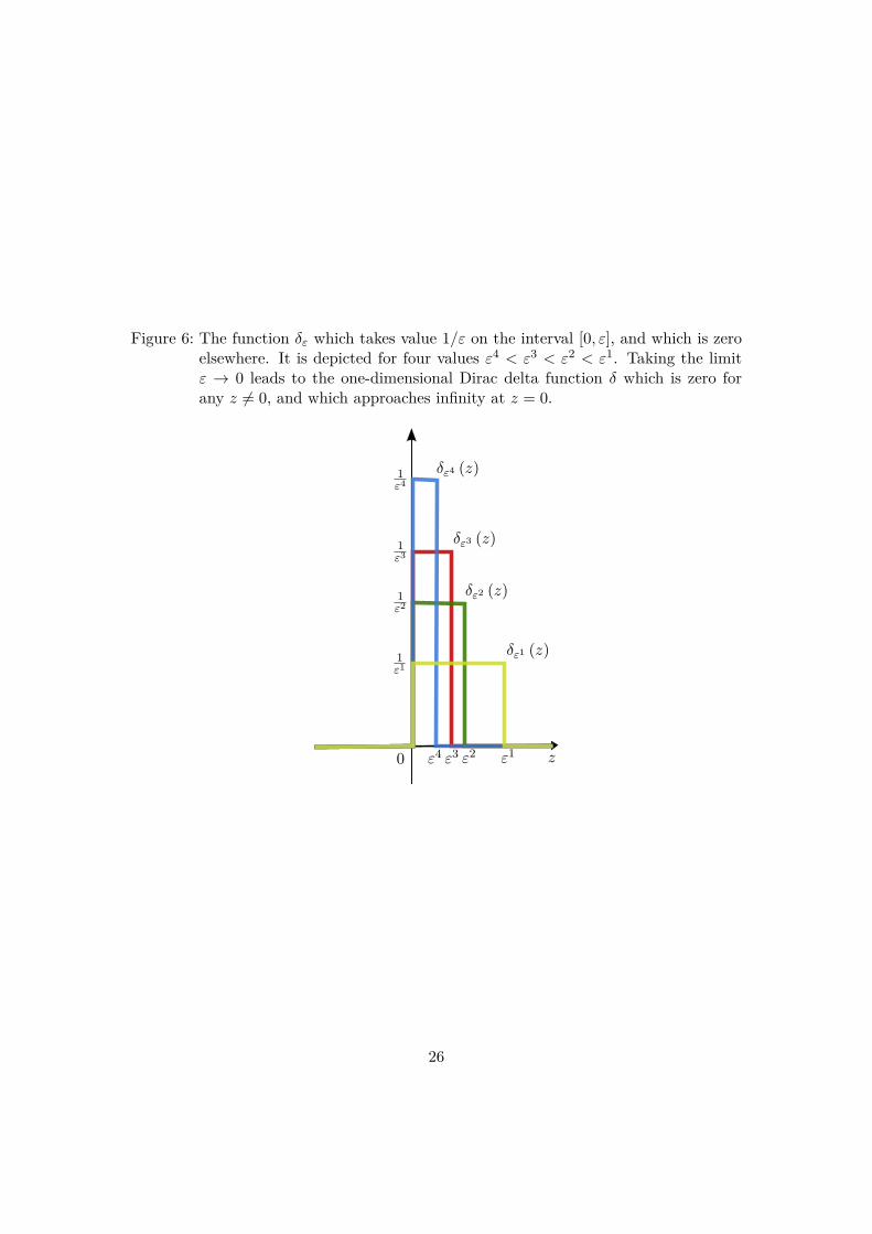
Figure 6: The function δε which takes value 1/ε on the interval [0, ε], and which is zeroelsewhere. It is depicted for four values ε4 < ε3 < ε2 < ε1. Taking the limitε → 0 leads to the one-dimensional Dirac delta function δ which is zero forany z 6= 0, and which approaches infinity at z = 0.
0 zε2
δε3 (z)
1ε2
ε1
1ε1
δε2 (z)
1ε3
δε4 (z)
ε3ε4
1ε4
δε1 (z)
26

Integrating a function g with δ (z − z′) dz′ as measure thus selects its value g (z).16
Now suppose that we can find a function G : R2 → R whose derivative is the Diracdelta:
∀z, z′ ∈ [z, z] : dG (z, z′)dz
≡ δ(z − z′
), (19)
and which complies to the following initial condition:
∀z′ ∈ [z, z] : G (z, z) ≡ 0. (20)
Then the following function solves differential equation (16):
B (z) ≡∫ z
zA(z′)G(z, z′
)dz′. (21)
To see this, take its derivative:
∀z ∈ [z, z] : dB (z)dz
= d
dz
[∫ z
zA(z′)G(z, z′
)dz′]
=∫ z
zA(z′) dG (z, z′)
dzdz′
=∫ z
zA(z′)δ(z − z′
)dz′
= A (z) ,
where I used the fact that the derivative can be brought inside the integral, and I useddefinition (19) and property (18). Furthermore, verify that indeed the initial conditionfor B is fulfilled:
B (z) =∫ z
zA(z′)G(z, z′
)dz′ = 0,
because of condition (20).It follows that finding a solution to a differential equation of form (16) boils down to
finding a function G which solves equation (19) and which complies to initial condition(20). Such a function is called a Green function of the problem.
I will now show that the Green function for the one-dimensional problem is the unitstep function.17 This function is defined as follows:
∀z, z′ : H(z − z′
)={
1 if z > z′,
0 if z ≤ z′.(22)
It immediately follows that it complies to initial condition (20):
∀z ∈ [z, z] : H (z − z) = 0.16This property is so fundamental that it is sometimes used as a defining property of the Dirac delta
function.17Again, see Arfken and Weber (2005) for a more traditional formulation of this property.
27

Furthermore, note that if we interpret δ (z) dz as a probability measure, then its cumu-lative distribution function is H (z):∫ z
−∞δ(z′′ − z′
)dz′′ = H
(z − z′
),
from the definition of the Dirac delta function. Take derivatives on both sides:
dH (z − z′)dz
= δ(z − z′
). (23)
We have thus found that the unit step function is the Green function for our problem.Substitute it into equation (21) to find the solution to differential equation (16):
B (z) =∫ z
zA(z′)H(z − z′
)dz′ =
∫ z
zA(z′)
dz′.
This is exactly the solution that we would have found by simply integrating the differ-ential equation. Applying it to the one-dimensional Euler-Lagrange equation (6) leadsto ABC-equation (8). I will extend this method to higher-dimensional problems in thefollowing subsections.
4.2. Two-Dimensional Tax BaseThe two-dimensional Euler-Lagrange equation (10) is a second-order partial differentialequation, subject to the boundary condition that the entity {∇xT (x) · xTl
(x) · x} fX (x)equals zero on the boundary Γ (X ) of the tax base space. Following the procedures forthe one-dimensional case, set forth in the previous subsection, I will treat this equationas if it were a first-order partial differential equation. In other words, I will solve apartial differential equation of the following form:
∀x ∈ X : A (x) =2∑l=1
∂Bl (x)∂xl
, (24)
with:
A (x) ≡ (1− α (x)) fX (x) , (25)
∀l : Bl (x) ≡
∑j
TjxjTl
fX (x) , (26)
subject to boundary conditions:
∀x ∈ Γ (X ) : B (x) · x = 0. (27)
28

Note that this formulation immediately leads to a transversality condition. Use thedivergence theorem to find:∫
XA (x) dx =
∫X
2∑l=1
∂Bl (x)∂xl
dx
=∫Γ (X )
B (x) · xdΓ
= 0,
or substituting (25) for A (x): ∫Xα (x) fX (x) dx = 1. (28)
This condition extends the notion, discussed by Jacobs (2013), that the marginal cost ofpublic funds equals one when the tax system is optimal.
To solve first-order partial differential equation (24), first introduce the two-dimensionalDirac delta function as the product of two one-dimensional Dirac delta functions:
∀x, y ∈ R2 : δ2 (x, y) ≡ δ (x) δ (y) . (29)
This function can again be constructed as the limit of a series of functions. I again usethe rectangular function for this purpose:
δ2ε
(x1, x2
)≡ δε
(x1)δε(x2)
={ 1ε2 if 0 < x1 < ε and 0 < x2 < ε,
0 elsewhere.
This function is depicted in figure 7. It integrates to one for any ε:∫ ∞−∞
∫ ∞−∞
δ2ε
(x1, x2
)dx1dx2 = 1. (30)
Take the limit ε→ 0 to find that δ2ε → δ2.
It is straightforward to check that property (18) extends to two dimensions. Integrat-ing a function g : R2 → R with measure δ2 (x− x′) dx′ selects its value g (x) :
∀x ∈ R2 :∫R2g(x′)δ2 (x− x′)dx′ = g (x) .
Like in the one-dimensional case described in the previous subsection, I will show thatfinding a solution to first-order partial differential equation (24) boils down to finding aGreen function G : R2 → R2 which solves the following partial differential equation:
∀x ∈ R2 : δ2 (x− x′) =2∑l=1
∂Gl (x,x′)∂xl
, (31)
complying to the following boundary condition:
∀x ∈ Γ (X ) ,∀x′ ∈ X : G(x,x′
)· x = 0. (32)
29

Figure 7: The function δ2ε which takes value 1/ε2 on the rectangle [0, ε]×[0, ε], and which
is zero elsewhere. Taking the limit ε → 0 leads to the two-dimensional Diracdelta function δ2 which is zero for all points besides the origin, and whichapproaches infinity at the origin.
1ε2
x1
δ2ε
(x1, x2)
x2
ε
ε
30

Note that the Green function G now is a vector-valued function, rather than a scalar-valued function as in the one-dimensional case.
If we find such a function G, then first-order partial differential equation (24) has thefollowing solution:
∀x, l : Bl (x) ≡∫XA(x′)Gl(x,x′
)dx′. (33)
This can be seen by substituting it into the right-hand side of partial differential equation(24), noting that the partial derivative can be brought inside the integral and usingproperty (30):
∀x :2∑l=1
∂Bl (x)∂xl
=2∑l=1
∂
∂xl
[∫XA(x′)Gl(x,x′
)dx′
]
=∫XA(x′) 2∑l=1
∂Gl (x,x′)∂xl
dx′
=∫XA(x′)δ2 (x− x′)dx′
= A (x) .
Verify that indeed the boundary conditions (27) are fulfilled, using condition (32):
∀x ∈ Γ (X ) ,∀x ∈ X : B (x) · x =∫XA(x′)G(x,x′
)· xdx′ = 0.
The question now is how to find the functions Gl that comply to partial differentialequation (31) with boundary conditions (32). I will state a solution here for the casewhere the tax base space equals the entire two-dimensional real vector space, X = R2. Iwill treat cases where the tax base set is a strict subset of the real vector space, X ( R2,e.g. excluding negative values, in section 6.
I will show that the Green function for this problem looks as follows:
∀x,x′ : G(x,x′
)≡ x− x′
D2 (x− x′) , (34)
where I introduce the two-dimensional distance function for any vector v in R2:
D2 (v) ≡ 2V 2 (||v||) ,
with V 2 (r) a function which maps a real number r on the surface area πr2 of a circlewith radius r, and with ||v|| ≡
√(v1)2 + (v2)2 the Euclidean norm, the “length” of the
vector v. After showing that this function indeed is a Green function, I will show howit leads to intuitive optimal-tax results.
31

First I need to show that the function (34) solves partial differential equation (31). Ishow in appendix B that it complies to the following properties:
∀x 6= x′ :2∑l=1
∂Gl (x,x′)∂xl
= 0, (35)
∀x′ :∫R2
( 2∑l=1
∂Gl (x,x′)∂xl
)dx = 1. (36)
These are the defining properties for the Dirac delta function. We conclude that thefunction G indeed solves partial differential equation (31).18
Next, note that the boundary conditions (32) are fulfilled:
∀x′ ∈ R2 : lim||x||→∞
G(x,x′
)· x = lim
||x||→∞
(x− x′) · x2π ||x− x′||2
= 0. (37)
It thus follows from (33) that the solution to partial differential equation (24) is asfollows:
∀x, l : Bl (x) =∫R2A(x′) xl − x′l
D2 (x− x′)dx′.
Substituting the definitions (25) and (26) for the functions A and Bl leads to optimal-taxcondition:
∀x, l :∑j
Tj (x)xjTl(x) fX (x) =
∫R2
(1− α
(x′)) xl − x′l
D2 (x− x′)dFX(x′). (38)
Using transversality condition (28), this equation can be simplified as follows:
∀x, l :∑j
Tj (x)XjTl
(x) = cov
(α(x′),
x′l − xl
D2 (x′ − x)
), (39)
where I introduce aggregate demand Xj (x) ≡ xj (x) fX (x) for tax base componentj at value x, and where Xj
Tl(x) ≡ xjTl
(x) fX (x) equals the sum of the compensatedresponses for the individuals pooling at tax base value x.19 The left-hand side in thisequation equals the compensated change in public revenues which is induced by a reformto the marginal tax rate Tl. It is the sum of the compensated effects on the differentcomponents of aggregate demand, multiplied by the respective marginal tax rates thatapply to these components. This side captures the efficiency effects of the reform.
The right-hand side captures the equity effects. It is a distance-weighted covariancebetween the average net marginal social welfare weight of the individuals pooling at taxbase value x with the value of the l − th component of the tax base. If the welfare18Partial differential equation (31) has multiple solutions. I argue in appendix B why solution 34 in the
one that we are interested in.19The entities Xj (x) and Xj
Tl(x) are density functions.
32

weights decrease strongly with the value of the tax base component, e.g. if individualswith higher gross labour income are weighted much less in the social welfare objective,then this covariance will be strongly negative. Balancing efficiency considerations againstequity considerations, the government will accept larger efficiency losses due to taxation,thus allowing the absolute value of the left-hand side of the equation to become larger.For given behavioural responses, high marginal tax rates will be warranted. However,if the welfare weights decrease less strongly, the absolute value of the covariance will besmaller, and optimal marginal tax rates will be lower.
The covariance term which captures the equity effects is distance-weighted. Whatmatters most is the covariance between the welfare weights and the tax base in theimmediate environment of the value of the tax base x under consideration. Figure 8ashows graphically the values of the distance weights: they become infinitely large inthe immediate environment of x and they decrease rapidly at slightly larger distances.Although the weights continue decreasing gradually at further distances, they only con-verge to zero at infinity. Figure 8b shows how the welfare weights are symmetric, in thesense that they depend only on the absolute value of the distance from the tax base levelunder consideration, independent of the direction.
We can reformulate equation (39) in a more familiar form. Denote the populationaverage of the net marginal social welfare weights as A ≡
∫X α (x′) fX (x′) dx′. This
quantity equals one in the optimum, by transversality condition (28). The optimal-taxcondition can then be rewritten as follows:
∀x, l :∑j Tj (x)X l
Tj(x)
X l (x) =cov
(α (x′) , x′l−xl
D2(x′−x)
)AX l (x) , (40)
where I use Slutsky symmetry XjTl
(x) = X lTj
(x). This is a different way of expressingthe government’s balancing exercise between efficiency and equity. The left-hand side ofthis equation is the proportional reduction of the l-th commodity along the compensateddemand schedule. The normalized covariance on the right-hand side is an extension ofthe distributional characteristic that was introduced by Feldstein (1972a,b).
This optimal-tax equation resembles closely a well-known result from the literature.Suppose that the government could not use the nonlinear, non-separable tax functionT , but instead it had to resort to separate linear tax rates tl. Adapting the results ofAtkinson and Stiglitz (1980, p.386-390) to my notations, denoting as X l the populationaggregate demand for the l-th component of the tax base, the optimal tax rates wouldbe determined by the following equation [TODO: do we really need the bar on X?]:20
∀l :∑j tjX
ltj
X l=
cov(α (x′) , x′l
)AX l
. (41)
The covariance on the right-hand side is again an extension of the distributional char-acteristic introduced by Feldstein (1972a,b). Since the different marginal tax rates are20This result is a bit simpler than the one found by Atkinson and Stiglitz (1980, p.388), since I allow
for a non-zero tax intercept. This implies that net social welfare weights average to one, similar totransversality condition (28).
33

Figure 8: The distance weight 1/D2 (x′ − x) ≡ 1/[2π((x1′ − x1)2 +
(x2′ − x2)2)] is a
measure of the inverted distance of a tax base value x′ to the value x. My ex-tended notion of the distributional characteristic is a normalized covariance ofthe average net marginal social welfare weights with the tax base components,distance-weighted by 1/D2.
(a) The weights are highest if the value x′ is close to x. There is a singularity at x′ = x. At valuesremoved from x this weight decreases, steeply so at closer distances, and more gradually further away.They converge to zero at infinite distance, without ever reaching it.
x2′
x2
1/D2 (x′ − x)
x1′
0
x
x1
(b) The distance weights 1/D2 are symmetric, in the sense that they depend only on the length ||x′ − x||of the vector x′ − x.
||x′ − x||
1/D2 (x′ − x)
0
34

now separable and constant, this equation is no longer specific to one value of the taxbase. Moreover, there is no distance weighting in the distributional characteristic. Myresult uses a localized distributional characteristic for each component of the tax base,whereas the result for linear tax rates uses global distributional characteristics. Result(40) is a direct extension of (41), from linear, separable tax rates to a non-separable,nonlinear tax function.
4.3. Higher-Dimensional CaseThe derivations for the higher-dimensional case are entirely analogous to those in the two-dimensional case. Again assuming that the tax base space coincides with the real vectorspace, X = RL, introduce the L-dimensional distance function DL (v) ≡ LV L (||v||),with V L (r) the volume of an L-dimensional sphere with radius r. The optimum canthen be formulated as in the following theorem.
Theorem 2. The tax optimum with an L-dimensional tax base with multidimensionalheterogeneity of the agents, in absence of bunching and when the tax base space coincideswith the real vector space, X = RL, complies to the following necessary condition:
∀x, l :
∑j
(Tjx
jTl
)fX
(x) = cov
(α(x′),
x′l − xl
DL (x′ − x)
), (42)
with transversality condition: ∫RLα (x) fX (x) dx = 1. (43)
Rewriting condition (42), it again follows that the proportionate reduction of ag-gregate demand along compensated demand curves should equal a distance-weighteddistributional characteristic, as stated in the following corollary.
Corollary 2. If we assume that we can use Slutsky symmetry xjTl= xlTj
and that the taxbase space coincides with the L-dimensional real vector space, X = RL, then in absenceof bunching the tax optimum complies to the following necessary condition:
∀x, l :∑j Tj (x)X l
Tj(x)
X l (x) =cov
(α (x′) , x′l−xl
DL(x′−x)
)AX l (x) . (44)
The interpretation of these results is entirely analogous to the two-dimensional case.It is a sufficient statistics formulation that can be applied to a wide range of problems,e.g. the joint progressive taxation of couples, the mixed nonlinear taxation of non-transferable commodities, the optimal mixed progressive taxation of labour income andcapital income, and so on. The necessary sufficient statistics can in principle be estimatedempirically.
A disadvantage of formulation (44) is that it obfuscates the underlying economics. It isnot clear how the Atkinson-Stiglitz result, which states that under a number of conditions
35

commodities should be taxed at uniform rates, could be derived from this equation, norhow it would follow that heterogeneous discount rates could lead to non-zero optimaltaxes on capital income. Moreover, if individuals would not report their true incomes,because they evade taxes or because they shift income between different bases, the formof the optimal-tax equation in terms of declared incomes would not change at all. Tostudy such questions, we need to delve deeper into the micro-foundations of the model.This will be the topic of the next section. But first I will apply the results of this sectionto the optimal taxation of couples.
4.4. Application to the Taxation of CouplesTo illustrate my result, let us consider the example of the optimal taxation of couples.Contrary to the example in subsection 3.4, I no longer impose boundaries on the taxbase space. Taxable incomes can become negative, and there is no conceptual differencebetween the primary and the secondary earner in the tax code. In order to guaranteethe anonymity of the members of the couple, they are randomly assigned to the first orthe second component of the tax base. The individuals earn gross incomes x1 and x2,summarized in the vector x. This procedure imposes symmetry on the welfare weightsand sufficient statistics, and thus on the tax function.21
Introduce the following aggregate tax elasticities:
∀l, j = 1, 2 : elj (x) ≡ − (1− Tj (x))xlTj
(x)xl
. (45)
Applying condition (44) then tells us that the following conditions are necessary for theoptimum:
∀x :
T1(x)
1−T1(x) e11 (x) + T2(x)
1−T2(x) e12 (x) = 1
fX (x)
cov(α(x′), x′1−x1
DL(x′−x)
)Ax1 ,
T1(x)1−T1(x) e2
1 (x) + T2(x)1−T2(x) e2
2 (x) = 1fX (x)
cov(α(x′), x′2−x2
DL(x′−x)
)Ax2 .
(46)
The left-hand sides contain the relative reductions of the tax bases. They are a measureof the distortions that are caused by the tax system. These quantities can in principlebe measured empirically. The same is valid for the density function fX .
The right-hand side contains the localized distributional characteristics of the respec-tive tax bases. Their values depend on the normative judgments of the government. Thegovernment could for example favour specialization within the couple, where one of bothpartners spends more time at home (e.g. caring for family members) while the othersupplies labour in the market. Alternatively, the government could favour equal sharingof both market and other activities, or it could not care at all about the distribution21Note that for the range x1 < x2, this setup must produce the exact same optimal tax function as the
setup where distinction is made between the primary and secondary earners, with xP ≥ xS . Thisobservation will play a central role in subsection 6.1, where I apply the method of images to deal withrestrictions to the tax base space.
36

within the family. Possibly the government would want to equivalize incomes, takinginto account scale effects from the size of the family. These important questions arebeyond the scope of this paper.22
5. Connection to Economic FundamentalsIn order to find more insight into optimal-tax equation (42), we need to restate ourresults in terms of the economic fundamentals of the problem. In the present section Ido this for the case where the dimension of the type space is equal to the dimension oftax base space, K = L. I assume that the allocation x (θ, T ) is a continuous, one-to-one function, strictly monotonous in all characteristics θk. I also assume that the taxfunction is smooth. I will extend these assumptions in section 6 about robustness.
I start in subsection 5.1 by restating the Euler-Lagrange equation in the type space,and I formulate the corresponding optimality conditions. Next I account for preferenceoptimization in subsection 5.2 to find a characterization of the optimum in terms ofeconomic fundamentals. I apply these findings to the joint taxation of couples in subsec-tion 5.3 . In subsection 5.4 I extend this characterization, allowing for a type-dependentindividual budget constraint, accounting e.g. for differences in bequests received by dif-ferent individuals. I demonstrate these results for the optimal mixed taxation of capitalincome and labour income in subsection 5.5.
5.1. Euler-Lagrange Formalism in the Type SpaceA first step to reformulate the tax optimum in terms of economic fundamentals is toreformulate Euler-Lagrange equation (12) as a partial differential equation in the typespace. Introduce the Jacobian matrix containing the partial derivatives of the allocation:
J ≡
x1θ1 (θ, T ) · · · x1
θK (θ, T )... . . . ...
xLθ1 (θ, T ) · · · xLθK (θ, T )
. (47)
This matrix extends the notion of a gradient to vector-valued functions. The follow-ing theorem then shows how the Euler-Lagrange equation for the tax optimum can bereformulated.22An important question, which I have been unable to solve, is what happens to the right-hand sides of
these equations as the value of a tax base component converges to infinity. Denote for example thelimit of α
(x1, x2) for x1 →∞ as α1+ (
x2). The right-hand side of the optimal-tax equation for thel-th component then becomes:
−α1+ (x2) ∫R2
x′l−xl
DL(x′−x) d(1− FX (x′)
)xlfX (x) .
The fraction in this equation appears to be a localized, multi-dimensional extension of the Pareto-term [1− F (x)] /xf (x) which occurs in the optimality condition for the one-dimensional problem(note that the divergence of
∫R2
[(x′ − x) /DL (x′ − x)
]d(1− FX (x′)
)equals −fX (x), just like
the derivative of 1− F (x) equals −f (x)). The precise interpretation of this term, and under whichcircumstances it converges to a constant value, as of yet remains unclear.
37

Theorem 3. Suppose the type space and the tax base space have equal dimensions, re-spectively K = L, and suppose that the mapping between both spaces is one-to-one. Thetax optimum, in absence of bunching, then complies to the following partial differentialequation, referred to as the Euler-Lagrange condition in the type space:
∀θ ∈ Θ : (1− α (x (θ, T ))) fΘ (θ) (48)
=K∑k=1
∂
∂θk
{[∇xT · x∇xT ·
(J −1
)ᵀ]k(x (θ, T )) fΘ (θ)
},
subject to the boundary conditions:
∀θ ∈ Γ (Θ) :{[
∇xT · x∇xT ·(J −1
)ᵀ](x (θ, T )) · θ
}fΘ (θ) = 0, (49)
and the government budget constraint:∫RK
T (x (θ, T )) fΘ (θ) dθ = 0. (50)
Proof. See appendix C.
The derivation of these equations is not so straightforward. The intuition though isclear. Since the instrument of our optimization is defined in the tax base space ratherthan the type space, we can not simply state a traditional Euler-Lagrange equation inthe type space. An additional term, the transpose of the inverse of the Jacobian matrix,needs to be added to account for the fact that we are working in a different vector space.The intuition of equation (48) remains the same as before: the social welfare effect ofa tax increase for all individuals of type θ, captured by the left-hand side, should beexactly compensated by the compensated effects experienced by the individuals in theimmediate environment of type θ, captured by the right-hand side.
The Euler-Lagrange equation (48) in the type space can be seen as a partial differentialequation of the same form as Euler-Lagrange equation (12) in the tax base space:
∀θ : A′ (θ) =K∑k=1
∂B′k (θ)∂θk
.
Assume now that the population density fX (x) is strictly positive for any x ∈ RL,so the tax base space coincides with the real vector space: X = RL. This means forexample that I do not exclude negative values of the tax bases. Using the same methodsas in section 4, we then find the tax optimum in the K-dimensional type space:
∀θ, k :[∇xT · x∇xT ·
(J −1
)ᵀ]k(x (θ, T )) =
cov(α(x(θ′, T
)), θ′k−θk
DK(θ′−θ)
)A θkfΘ (θ) . (51)
This equation again reflects the balancing exercise between efficiency and equity. Theright-hand side captures the equity aspects of the government’s balancing exercise.
38

Rather than being a distributional characteristic of a component of the tax base though,it is now a distributional characteristic for the k-th component of the type of the in-dividuals. Is is an indication of how much the government cares about that particularindividual trait. Perhaps it values more highly individuals with a lower ability, individ-uals who are more willing to work, or those who receive a lower inheritance. Again thisdistributional characteristic is localized around the type θ under consideration, weightedby distance function 1/DK , with a similar interpretation to that formulated in section4.
The term x∇x (x (θ, T )) on the left-hand side is an indication of how strong be-havioural responses are when there is a change to the gradient of the tax function.The inverse J −1 of the Jacobian matrix indicates how the types θ are related to thetax base values x. If we slightly change the tax base value x that we are studying, thenthere is a change in the underlying type θ that is choosing the tax base value underconsideration, determined by the elements
(xlθk
)−1of the inverted Jacobian matrix.23
The product x∇x (x (θ, T ))·(J −1)T combines these two terms to give information about
how strong is the change in the type choosing an allocation x, if the tax gradient at thatpoint changes:
x∇T (θ, T ) ·(J −1
)ᵀ= − dθ
d∇xT (x (θ, T ))
∣∣∣∣ᵀx
.
Formally this property follows from the analytic implicit function theorem, which is amultidimensional extension of the implicit function theorem in one dimension.
Substituting this relation into Euler-Lagrange equation (51) in the type space leadsto an interesting reformulation of our optimal tax condition:
∀θ, k : −∑l
Tl (x (θ, T ))θkfΘ (θ) · dθk
dTl (x (θ, T ))
∣∣∣∣∣x
fΘ (θ) =cov
(α(x(θ′, T
)), θ′k−θk
DK(θ′−θ)
)A θkfΘ (θ) . (52)
The left-hand side contains the proportional change in the k-th component of the typeresiding at the value of the tax base under consideration. The term dθk/dTl
∣∣∣x
tells ushow the k-th component of the type of the individuals choosing tax base x changes whenthere is a reform of the l-th component of the tax gradient. The larger is this term, theless able will be the government to target this trait using this component of the taxbase. The left-hand side in its entirety is an indication of the cost that is associated torevealing information about that characteristic of the individual.
Optimal-tax condition (52) then shows how the government faces a balancing exercisebetween the social advantage of redistribution between individuals with different valuesof the trait θk, against the cost of targeting that trait.
Even though equation (52) has an intuitive interpretation, and even though it involvesinformation about the types that cannot be observed by the government, it is still for-mulated in terms of summary statistics, which depend on the underlying behavioural23The inverse function theorem states that the elements of the inverse of the Jacobian matrix are the
inverses of the elements of the original Jacobian matrix.
39
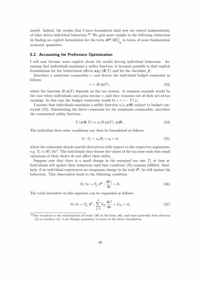
model. Indeed, the results that I have formulated until now are stated independentlyof what drives individual behaviour.24 We gain more insight in the following subsectionby finding an explicit formulation for the term dθk/dTl
∣∣∣x
in terms of more fundamentaleconomic quantities.
5.2. Accounting for Preference OptimizationI will now become more explicit about the model driving individual behaviour. As-suming that individuals maximize a utility function, it becomes possible to find explicitformulations for the behavioural effects x∇T (θ, T ) and for the Jacobian J .
Introduce a numeraire commodity c, and denote the individual budget constraint asfollows:
c = B (x|T ) , (53)
where the function B (x|T ) depends on the tax system. A common example would bethe case where individuals earn gross income z, and they consume out of their net-of-taxearnings. In this case the budget constraint would be c = z − T (z).
I assume that individuals maximize a utility function u (c,x|θ) subject to budget con-straint (53). Substituting the latter constraint for the numeraire commodity, introducethe constrained utility function:
U (x|θ, T ) ≡ u (B (x|T ) ,x|θ) . (54)
The individual first-order conditions can then be formulated as follows:
∀l : Ul = ucBl + ul = 0, (55)
where the subscripts denote partial derivatives with respect to the respective arguments,e.g. Ul ≡ ∂U/∂xl. The individuals thus choose the values of the tax base such that smallvariations of their choice do not affect their utility.
Suppose now that there is a small change in the marginal tax rate Tj at base x.Individuals will update their behaviour such that condition (55) remains fulfilled. Simi-larly, if an individual experiences an exogenous change in his trait θk, he will update hisbehaviour. This observation leads to the following condition:
∀l,∀ν = Tj , θk : dUl
dν= 0. (56)
The total derivative in this equation can be expanded as follows:
∀l,∀ν = Tj , θk :
L∑j=1
Uljdxj
dν+ Ulν = 0. (57)
24One exception is the reformulation of result (39) in the form (40), and more generally from theorem(2) to corollary (2). I use Slutsky symmetry to arrive at the latter formulation.
40

Define the Hessian H of U as the matrix containing its second-order partial derivatives:
H ≡
U11 · · · U1L... . . . ...
UL1 · · · ULL
.This allows rewriting result (57) in matrix notation:
∀ν = Tj , θk : dx
dν= −H−1 · Uxν ,
where I multiply both sides from the left by the inverse of the Hessian.It now follows that the Jacobian matrix is given by:
J = −H−1 · Uxθ, (58)
and the matrix with compensated effects looks as follows:
∀l : xTl= −H−1 · UxTl
. (59)
Before applying these results, I will give more explicit formulations for the terms UxTl
and Uxθ. First assume that there is a reform to the marginal tax rate of size dTj at taxbase value xR, keeping constant the liability at xR itself. Denoting by x the value ofthe tax base chosen after the reform by someone who originally chooses xR, we obtaina new budget constraint:
c = B (x|T )−(xj − xR,j
)dTj .
It is clear that when the individual does not change his behaviour, xj = xR,j , his taxliability remains unaltered. The change in the marginal tax rate applies only to hisresponses to the reform. Note that taking the derivative of this budget constraint, forgiven value of the tax base, yields the following relation:
dc
dTj
∣∣∣∣∣x
= −(xj − xR,j
).
Using definition (54) we now find:
UlTj= ∂
∂xl
(uc
dc
dTj
∣∣∣∣∣x
)= − ∂
∂xl
(uc(xj − xR,j
)). (60)
Evaluating this expression in the situation with no tax reform, when xj = xR,j , it follows:
UlTj={−uc if l = j,
0 if l 6= j.(61)
41

Similarly, again using definition (54):
Ulθk = ulθk + ucθkBl = ulθk − ucθk
uluc
= uc∂ (ul/uc)∂θk
∣∣∣∣x, (62)
where I substitute individual first-order condition (55) in the second step.Substituting results (58), (59), (61), and (62) into optimal-tax condition (51) then
yields the following necessary condition for the optimum:
∀θ, l : Tl (x (θ, T )) (63)
=− 1fΘ (θ)
∑k
∂ (ul/uc)∂θk
∣∣∣∣x
cov
(α(x(θ′, T
)),
θ′k − θk
DK(θ′ − θ
)) .This equation is a direct extension of a result obtained by Mirrlees (1976) for the casewith a one-dimensional type space.25 The l-th component of the optimal tax gradient,Tl, is higher for a particular type θ if there are fewer individuals at that point whosebehaviour is impacted, or if the government particularly values compensation for traitsthat can be better targeted using that component of the tax base.
To gain more intuition about the term ∂ (ul/uc) /∂θk∣∣∣x, consider for example the
following Atkinson-Stiglitz (1976) type of model with one-dimensional type n. Supposeindividuals with ability n supply labour `, which yields earn gross labour income z = n`.They consume a numeraire good c and a taxed good y. They maximize utility u
(c, y, zn
),
subject to budget constraint c = z − p · y − T (z, y), with p the producer price of goody. We are now interested in the following term:
∂ (uy/uc)∂n
∣∣∣∣z,y
= − `n
1uc
[uy` − uc` (p+ Ty)] ,
where I substitute the first-order condition uy = (p+ Ty)uc on the right-hand side. Itimmediately shows that when preferences are separable between leisure and consump-tion, such that uy` = uc` = 0, this expression becomes zero. Conditional on the tax base(z, y), the marginal rate of substitution uy/uc does not reveal any information about theindividual type, and there is no point in taxing good y. Doing so would introduce a dis-tortion, without introducing the counterbalancing advantage of being able to differentiatebetween individuals with different abilities. If, on the other hand, utility is not separa-ble, then equation (63) tells us that the marginal tax rate on y will be higher when theterm ∂ (uy/uc) /∂n|z,y is larger, as suggested by Corlett and Hague (1953). Optimal-taxcondition (63) shows how this reasoning extends to multi-dimensional characteristics.
5.3. Application to Taxation of CouplesI will now apply the findings of the previous subsection to the optimal taxation ofcouples, following a model introduced by Kleven, Kreiner, and Saez (2007). Let each25The difference with the formulation by Renes and Zoutman (2016a) stems from the fact that the net
social welfare weight α already incorporates the income effects. This makes that formulation (63)has a more intuitive interpretation.
42

couple consist of two individuals with respective labour abilities n1 and n2, with domain[n1, n1]× [n2, n2]. As before, labour supply of the individuals is denoted by `1 and `2,
and the corresponding gross labour incomes are z1 and z2. The budget constraint forthe household is given as follows:
c = z1 + z2 − T(z1, z2
).
Utility is separable, and linear in consumption:
u
(c,z1
n1 ,z2
n2
)≡ c− n1h1
(z1
n1
)− n2h2
(z2
n2
).
Define the following elasticities:
εk ≡ 1− Tkzk
∂zk
∂ (1− Tk)=
hk`k
`khk`k`k
.
The effect of the respective abilities on the marginal rates of substitution then look asfollows:
∂ (uz1/uc)∂n2
∣∣∣∣z
= ∂ (uz2/uc)∂n1
∣∣∣∣z
= 0,
∂ (uz1/uc)∂n1
∣∣∣∣z
= 1ε1 ,
∂ (uz2/uc)∂n2
∣∣∣∣z
= 1ε2 .
Substituting these results into equations (58), (59), (61), and (62), and applying theorem3, yields the following divergence equation for the tax optimum:
∀n1, n2 : (α− 1) fΘ(n1, n2
)= ∂
∂n1
(T1
1− T1
h1`1
`1h1`1`1
n1fΘ(n1, n2
))(64)
+ ∂
∂n2
(T2
1− T2
h2`2
`2h2`2`2
n2fΘ(n1, n2
)).
This is exactly the optimality condition found by Kleven, Kreiner, and Saez (2007) intheir proposition 4. Using the methods in the present paper, we can now state theoptimum for the case where the domain of the skills coincides with the real vector spaceR2:
∀k : Tk1− Tk
= 1εk
cov
(α′,
n′k − nk
D2 (n′1 − n1, n′2 − n2)
)1
nkfΘ (n1, n2) . (65)
This solution, to the best of my knowledge, had not been stated before in the literature.Furthermore, apply theorem 3 to find the following boundary conditions:
∀k : ∀nk = nk, nk :{
Tk1− Tk
εknkfΘ(n1, n2
)}= 0.
This again confirms the findings stated by Kleven, Kreiner, and Saez (2007) in theirproposition 4.
43

5.4. Type-dependent Budget ConstraintMuch of the optimal-tax literature, including the contributions of Mirrlees (1971), Mir-rlees (1976) and Atkinson and Stiglitz (1976), assumes that the budget constraint doesnot depend directly on the individual traits. Still it is interesting to allow for this pos-sibility. It is possible for example that individuals receive an unobserved inheritance, asstudied by Cremer, Pestieau, and Rochet (2001), or that they receive a skill-dependentreturn on their investment, as described by Gerritsen et al. (2015).
Assume thus that the individual budget constraint can be expressed as follows:
c = B (x|θ, T ) .
For example, suppose that individuals have gross labour income z, and they receive anunobserved bequest b. In this case the budget constraint would be c = z − T (z) + b.
The derivations from subsection 5.2 remain valid. The value (62) of second-orderpartial derivative Ulθk changes though:
Ulθk = uc∂
∂θk
[uluc
(B (x|θ, T ) ,x|θ) +Bl
]∣∣∣∣x.
Note that in the argument of the marginal rate of substitution ul/uc, I substitute thebudget constraint for the numeraire. This formulation takes into account the effectsof the changes in the type on the budget constraint. The term within square bracketsindicates how strongly the individual marginal rate of substitution would deviate fromits optimum if there were an exogenous change in his trait θk, if the individual wouldnot alter his behaviour.
Optimal-tax condition (51) then becomes:
∀θ, l : Tl (x (θ, T )) = − 1fΘ (θ)
∑k
∂
∂θk
[uluc
(B (x|θ, T ) ,x|θ) +Bl
]∣∣∣∣x
(66)
· cov
(α(x(θ′, T
)),
θ′k − θk
DK(θ′ − θ
)) .The intuition is similar to that in subsection 5.2. The l-th component of the tax
gradient is higher for a particular type θ if there are less individuals whose behaviouris affected. It is also higher if the government cares more about traits which have astronger influence on the marginal rate of substitution in the direction of that tax basecomponent – now taking into account the effect of a change in the type on the individualbudget constraint. If a small change in an individual trait causes a strong deviationin a particular direction of the tax base, then the government can use that tax basecomponent more easily to target that particular characteristic.
5.5. Application to Mixed Taxation of Labour and Capital IncomesI will apply the findings from the previous subsection to the optimal mixed taxation ofcapital income and labour income. I will describe a model where individuals differ in two
44

dimensions: they have different labour productivities n, and they have different discountrates ρ. This distinction was also made by Diamond and Spinnewijn (2011), who finddesirability conditions in a model with just two or three values of each characteristic. Iextend their model here to continuous characteristics. Moreover, to be able to demon-strate my findings for a type-dependent budget constraint, I assume that more patientindividuals obtain higher returns on their savings, and that more able individuals obtainhigher returns.
There are two periods in the model. In the first period, individuals supply labour`, which yields a gross income z ≡ n`, they consume an amount c1, and they save anamount a. Their savings yield a gross capital income y ≡ aR (n, ρ), which depends onthe amount saved and on the discount rate and the ability of the individual.
In order to keep the model tractable, I assume that individuals pay a tax T (z, y) atthe end of the first period. It depends on their labour income and their capital income.Their first-period budget constraint thus looks as follows:
c1 + a+ T (z, y) = z.
Second-period consumption then equals the amount saved, plus the capital income ob-tained from it:
c2 = (1 +R (n, ρ)) a.
To be able to apply the findings of the previous subsection, I write the intertemporalbudget constraint in terms of the tax bases:
c1 = B (z, y|n, ρ, T ) ≡ z − T (z, y)− y
R (n, ρ) .
Individuals obtain utility from their first-period and their second-period consumption,and they experience a disutility from their labour supply. I immediately write the utilityfunction in terms of the numeraire commodity c1 and the values of the tax base:
u(c1, z, y|ρ, n
)≡ v
(c1)
+ ρv
([ 1R (n, ρ) + 1
]y
)− w
(z
n
).
Preferences are thus intertemporarily separable, and they are separable between leisureand consumption. This allows deriving the first-order conditions:
0 = uzuc1
(B (z, y|n, ρ, T ) , z, y|n, ρ) =(1− T ′
)− 1n
w`vc1
, (67)
0 = uyuc1
(B (z, y|n, ρ, T ) , z, y|n, ρ) = −(Ty + 1
R (n, ρ)
)+ ρ
vc2
vc1
(1 + 1
R (, nρ)
). (68)
The relevant derivatives of the budget constraint are as follows:
Bzn = Bzρ = 0, Byn = RnR2 , Byρ = Rρ
R2 . (69)
45

and the relevant derivatives of the marginal rates of substitution:
∂
∂ρ
(uzuc1
)∣∣∣∣z,y
= 0, (70)
∂
∂n
(uzuc1
)∣∣∣∣z,y
= 1n
w`nvc1
(1 + w```
w`
), (71)
∂
∂ρ
(uyuc1
)∣∣∣∣z,y
= RρR2 + vc2
vc1
(1 + 1
R (ρ)
)− ρvc2
vc1
RρR2
[1 +
(1 + 1
R (, nρ)
)vc2c2
vc2
], (72)
∂
∂n
(uyuc1
)∣∣∣∣z,y
= RnR2 − ρ
vc2
vc1
RnR2
[1 +
(1 + 1
R (, nρ)
)vc2c2
vc2
]. (73)
We now have the necessary elements to derive the optimal-tax equations. First applyoptimal-tax condition (66) to find the optimal marginal tax on labour income:
∀θ : Tz1− Tz
= 1nfΘ (n, ρ)
(1 + w```
w`
)cov
(α(n′, ρ′
),
n′ − nD2 (n′ − n, ρ′ − ρ)
),
where I used first-order condition (67) to rearrange some terms. The first two terms onthe right-hand side of this equation look a bit similar to the result found by Mirrlees(1971). The first term incorporates properties of the skill distribution, and the sec-ond term is the inverse of the Frisch elasticity of labour supply (controlling for capitalincome). The third term though looks completely different in this case. Rather thanlooking at the net social welfare weights of all individuals with higher skills, and weighingthem equally, as in the B-term in equation (8), it now incorporates a distance-weightedcovariance of the net social welfare weights with the tax base. The distance-weightingis symmetric, and also tax base levels below the tax base under consideration contributeto the optimal tax on labour income.
For the optimal tax on capital income we obtain the following equation:
∀θ : fΘTy =−[∂
∂ρ
(uyuc1
)∣∣∣∣z,y
+Byρ
]cov
(α(n′, ρ′
),
ρ′ − ρD2 (n′ − n, ρ′ − ρ)
)
−[∂
∂n
(uyuc1
)∣∣∣∣z,y
+Byn
]cov
(α(n′, ρ′
),
n′ − nD2 (n′ − n, ρ′ − ρ)
).
We can learn a number of things. Note first that if the discount rates are not hetero-geneous, then the covariance on the first line will be zero. Assume that the covarianceon the second line is not zero, e.g. because the government would like to redistributeaway from individuals with high innate abilities. The only reason then why the optimalmarginal tax rate on capital income might differ from zero, in this model, is that theterm within square brackets on the second line differs from zero. This is the case whenan exogenous change in the labour ability n of an individual, somehow causes his savingsno longer to be in optimal in his original bundle. My model is such that preferencesbetween leisure and consumption do not depend directly on labour ability. One reason isthat I assumed separability between leisure and consumption, thus excluding the motives
46

found by Corlett and Hague (1953). Another reason is that I exclude direct dependenceof the discount rate on labour ability (ρ 6= ρ (n)), thus excluding the motives foundby Saez (2002). Still, if the interest rate obtained by the individuals is skill-dependent(Rn 6= 0), this term will differ from zero because of results (69) and (73), and the optimalmarginal tax on capital income will differ from zero. This complements the findings ofGerritsen et al. (2015). It is thus important not only to take into account the directimpact of the traits on individual preferences, but also to take into account the effectson the individual budget constraint.
If neither of above reasons is true, then the second line will be zero. Still there mightbe reasons to tax capital income. If not all individuals have the same discount rate,then by definition the marginal rate of substitution between the two periods will dependon it. The term between square brackets on the first line thus differs from zero. If thecovariance between the welfare weights and the discount rates differs from zero, thenthe optimal marginal tax rate on capital income will differ from zero, confirming thefindings of Diamond and Spinnewijn (2011). Furthermore, if the rates of return R (n, ρ)depend directly on the discount rate, such that more patient individuals obtain higherreturns, this further affects the value of the term between square brackets on the firstline, further contributing to a non-zero optimal tax on capital income. Again it turnsout to be important to incorporate the effects of the individuals traits on their budgetconstraints.
Note that even when the second line in this optimal-tax equation is zero, and evenwhen the welfare weights are forced to be independent of the discount rate becauseindividuals are held responsible for their own preferences (so αρ = 0), even then thefirst line on the right-hand side might differ from zero, for the mere reason that thediscount rates ρ are locally correlated with the labour skills n. So, even if we deem thepreference for savings to be irrelevant for moral reasons, still we might end up using itto differentiate between individuals because it contains imperfect information about theinnate abilities.
6. RobustnessThere are a number of circumstances where the assumptions of the above derivations areviolated. For example, I always assumed that the relevant functions and their derivativesare sufficiently smooth. When characterizing the optimum in section 4, I assumed thatthe tax base space spans the entire real vector space. And when connecting to economicfundamentals in section 5, I assumed that each allocation in the tax base space waschosen by exactly one type.
There are a number of ways in which these conditions may be violated. A first possi-bility is that the tax base space is restricted, for example because there are some legal orphysical restrictions on the values that the tax base may take. It may be impossible toconsume negative quantities of certain goods, or it may not be allowed to report negativevalues. When characterizing the optimum in section 4, I used the assumption that thetax base space coincides with the entire real vector space (X = R2), so I could use Green
47

functions with boundary conditions for ||x|| → ∞. I will argue in subsection 6.1 thata restricted tax base space impels us to add some correction terms to the optimalityconditions.
Another possible violation of my assumptions occurs when the type space has a higherdimension than the tax base space. In this case individuals of different types will in-evitably pool at the same allocation, even when a strict monotonicity assumption ismaintained for the allocation, i.e. ∂xl/∂θk > 0 for all components. For example, for agiven gross labour income, one might simultaneously observe talented individuals whoprefer to work fewer hours, and less productive individuals who prefer to work morehours. This possibility is allowed for by the Euler-Lagrange equation in theorem 1 andthe characterization of the optimum in terms of sufficient statistics in equation (44),where behavioural responses are averaged over the individuals pooling at the tax basevalue under consideration, but section 5 explicitly excludes this possibility when it as-sumes a one-to-one allocation. Subsection 6.2 explains how to deal with this.
Another situation where individuals of different types choose the same allocation, iswhen bunching occurs. Consider an infinitesimal volume dx around a tax base valuex. The number of individuals choosing a value in that volume equals f (x) dx. If weshrink this volume to a single point, dx → 0, then in absence of bunching the numberof individuals in it will converge to zero. Since any real volume contains infinitely manypoints, removing a single point will not make a difference when we integrate over thatvolume. We say that a volume of measure zero contains a zero mass of individuals.The situation changes when there is bunching. Suppose for example that 10% of thepopulation chooses not to work: they choose the corner solution z = 0. Then the numberof individuals bunching on an infinitesimal interval dz around labour income z = 0,f (0) dz, will converge to 10% as dz → 0. For this to be possible, there needs to be aninfinite spike in the density function at z = 0. We say that there is a mass of individualsbunching at this point. The density function makes a discontinuous jump at the edge,and the objective function is no longer sufficiently smooth for my derivations to holdwithout modifications. Seade (1977) shows how in this situation the zero-marginal-taxresult at the bottom disappears. I study this possibility in subsection 6.3.
Bunching may also occur at an interior point of the tax base space. Ebert (1992)gives an example for the labour income tax with a utilitarian government objective,where individual preferences and the skill distribution coalesce such that the individualsecond-order conditions become binding at a some range of skills. Mirrlees (1976) showsthat with a one-dimensional type θ, when a single-crossing condition is fulfilled forthe indifference curves, the individual second-order condition is equivalent to the weakmonotonicity condition dz/dθ ≥ 0. If this condition is binding, so dz/dθ = 0, it followsthat a range of individuals of consecutive skill levels will bunch at the same labourincome.
Bunching differs from pooling. In the case of bunching, the strict monotonicity condi-tion is violated: individuals of consecutive types choose the same allocation, forming amass point. In the case of pooling, the strict monotonicity condition remains satisfied; itusually occurs when the type space has a higher dimensionality than the tax base space.There is no infinite spike in the density function, and thus there is no mass point in the
48

income distribution.Kleven, Kreiner, and Saez (2007) show for the nonlinear joint taxation of couples,
that the no-bunching assumption is reasonable for a wide range of social objectives. Stillthere are cases where bunching is important. One example is the Rawlsian objective,where all weight falls on a single individual. Another example where bunching mayoccur is the case where most weight is given to a type in the interior of the type space(e.g. attaching a higher social welfare weight to the working poor than to those out ofwork).26
An optimal allocation that includes an interior bunching range, is implemented usinga kinked tax function. That is, the tax function itself remains continuous, but thereis a discontinuity in its gradient. Suppose for example with a one-dimensional labourincome tax base, that at a given point the marginal tax rate jumps from 40% to 45%.Individuals with a marginal rate of substitution between labour income and consumptionlower than 40% (− (1− T ′) < −60%) will choose a labour income below the kink, whileindividuals with a marginal rate of substitution above 45% (− (1− T ′) > −55%) willchoose a labour income above the kink. Those with a marginal rate of substitutionbetween 40% and 45% will bunch at the kink. There will be a mass of individuals atthat point. Again the objective function is no longer sufficiently smooth and I need toadapt my derivations. I do so in subsection 6.3.
Another difficulty occurs when the dimension of the type space is lower than thedimension of tax base space. This is typically the case in the literature that studiesproblems involving multidimensional tax bases with one-dimensional types. Examplesinclude the seminal papers of Mirrlees (1976) and Atkinson and Stiglitz (1976). Inthis case the allocation forms a one-dimensional path in a multidimensional tax basespace. A typical complication in this case, when solving the optimal-tax problem usingthe mechanism design approach, is that of double deviations. The problem is that theincentive compatibility constraint that is taken into account, guarantees only that eachindividual chooses the bundle that is meant for him among the bundles that are situatedon that one-dimensional path. If the optimum is decentralized though using a taxsystem, there is no a priori reason why an individual would not prefer a bundle thatis situated outside the one-dimensional allocation. Most authors, to circumvent theproblem, simply set the tax liability infinitely high at these alternative values (see e.g.Rochet, 1985). Renes and Zoutman (2016b) show that it suffices that the individualsecond-order conditions for the decentralized optimization problem are fulfilled in thebundles that are assigned to the different types: it suffices that the tax liability increasesstrong enough when individuals deviate from the one-dimensional path of the allocation,to discourage them from doing so.
In my approach, where we are given a tax function with corresponding density func-tions and marginal behavioural responses, the problem of double deviations becomes26Armstrong (1996) and Rochet and Chone (1998) study the problem of a monopolist choosing nonlinear
prices for a set of potential qualities of its product. They show that when individuals choose whichqualities to buy, and they have an option not to buy the product at all, then the presence of bunchingcannot be ruled out without making unreasonable assumptions. These results are less relevant forthe present paper, as I rule out the existence of an outside option.
49

irrelevant. If we observe an income distribution corresponding to a given tax function,that means that individuals have already chosen their tax base values, conforming totheir incentives. If we observe that individuals pool on a one-dimensional allocation,that automatically implies that the second-order conditions given by Renes and Zout-man (2016a) are fulfilled on that line. Still, I cannot simply ignore the this case: Ineed to demonstrate how the multidimensional optimal-tax equation (42) collapses tothe more traditional equations found e.g. by Mirrlees (1976) and Atkinson and Stiglitz(1976). This will be the topic of subsection 6.4.
6.1. Tax Base RestrictionsThe optimal-tax condition in theorem 2 is based on the assumption that the tax basespace coincides with the real vector space: X = RL. As mentioned, the tax base spacemight be limited to a subset, e.g. for legal or physical reasons. One typical example isthat one or more components of the tax base are restricted to be non-negative. Anotherrelevant example is the joint taxation of couples, where both partners should be treatedanonymously. As explained in subsection 3.4, the latter limits the tax base space to abisection of the real space.
Theorem 2 is no longer correct when the tax base space is limited to a subset of RL.The reason is that it is based on a Green function of the form in equation (34). Theproblem is that the boundary condition (37) is no longer fulfilled when the boundary issituated at finite values of the tax base.
Remember how in subsection 4.4 for the joint taxation of couples, I got rid of thelimitation that the income of the primary earner should be higher than the income ofthe secondary earner, by randomly assigning the partners in each couple to either the firstor the second position in the definition of the tax base. This led to symmetric sufficientstatistics, and if the welfare weights respected anonymity, it led to a tax function whichwas symmetric in the identity of the individuals. Using this procedure, the domain ofthe problem was extended to include the entire real vector space, rather than the halfwhere the primary earner had a higher income than the secondary earner. We were thusable to solve the problem using theorem 2, based on a Green function with boundaryconditions at infinite levels of the tax base.
The procedure set forth in subsection 4.4 is an application of a more general method,the method of images. I created an image of the economy under consideration wherethe values of zP and zS were switched for all individuals. This method is typically usedin combination with Green functions, e.g. to solve problems in the field of electromag-netism. I will attempt to explain the solution procedure in economics terms. A moretraditional treatment of the subject can be found e.g. in Lax et al. (1998, p.235-238).
I will focus on a two-dimensional tax base with values x ≡ (z, y), where y can takeany value, but z is restricted to non-negative values (z ≥ 0). The tax base spacethus coincides with a half plane in the real vector space: X ≡
{x ≡ (z, y) ∈ R2|z ≥ 0
}.
Theorem 1, stating the Euler-Lagrange equation, remains valid, but we can no longeruse theorem 2 to characterize its solution.
The trick to solve this problem is again to create an image of this economy. Assign
50

Figure 9: The tax base space X is limited to those points (z, y) ∈ R2 which have non-negative values of z. The fact that X does not coincide with R2 makes thatwe can no longer apply theorem 2. A solution is to create an “image world”, amirror image of the true economy around the line z = 0. The tax base spaceof this image world has elements
(zi, yi
)∈ X i, with non-positive values for zi.
Since the union X ∪X i coincides with R2, we can use theorem 2 to optimizethe tax function on this extended economy. The values of this optimal-taxfunction on the set X coincide with the solution for the original problem.
z
y
X ≡{(z, y) ∈ R2|z ≥ 0
}
x′ = (z′, y′)
∇T (x′)
x′∇T
xi = (−z′, y′)
∇T(xi)
xi∇T
X i ≡ {(−z, y) | (z, y) ∈ X }
Image of theTax Base Space Tax Base Space
0
all units in the population randomly to one of two groups. The first group reports theirtrue gross income as usual, but the second group reports a negative value of z. For amember of the second group, if his tax base originally took the value x′ = (z′, y′), hewill now report the image value xi = (−z′, y′). Now let the government optimize a newtax function on this extended domain. The new tax base space coincides with the entirereal vector space R2, as illustrated in figure 9.
The derivations in section 3 are valid in this case. Implementing a localized reformsimilar to those used in subsections 3.1 and 3.2, should still leave social welfare un-changed. Theorem 1 remains valid, and the Euler-Lagrange equation looks exactly thesame.27 What is more, since the image economy is the exact mirror of the original econ-omy, the optimal tax function on the extended domain should be symmetric around theline defined by the equation z = 0. It follows that the entity ∇xT (x′) ·x∇xT (x′) shouldbe the exact mirror of the entity ∇xT
(xi)· x∇xT
(xi).
Now consider a point x ≡(0, y
)which lies on the line z = 0. Note that this point
is necessarily equal to its image: x = xi. It follows that the vector ∇xT (x) · x∇xT (x)27I ignore the fact that the density function is halved, since half of the population is moved to the image
world. The factor 1/2 drops out in all results anyway.
51

should be equal to its own image. The only way that this is possible, is that it is parallelto the line z = 0. It follows that in the optimum, necessarily ∇xT (x) ·x∇xT (x) · x = 0.This is exactly the requirement of boundary condition (13) in theorem 1.
If we can thus solve this new problem on domain R2, then we have a tax functionwhich conforms to all conditions of theorem 1. We thus immediately obtain a solutionfor the original problem, by using the values of the optimal tax function on the positivehalf of R2.
The solution to the original optimal tax problem thus looks as follows:
∀x ∈ X , l :∑j
(Tj (x)xjTl
)fX (x) (74)
= covX
(α(x′),
x′l − xl
D2 (x′ − x)
)+ covX
(α(x′),
xil − xl
D2 (xi − x)
).
To see more formally that this solution is correct, note that this is the solution thatwe would have found if I had used the following Green function in subsection 4.2:
G(x,x′
)≡ x− x′
D2 (x− x′) + x− xi
D2 (x− xi) .
If I can show that this Green function fulfills conditions (31) and (32), then I haveformally shown the validity of solution (74).
The derivations in appendix B lead to the following property:
∑l
∂Gl (x′,x)∂xl
= δ2 (x′ − x)+ δ2(xi − x
).
Since for all elements x in the tax base space X we necessarily have xi 6= x, the secondterm on the right-hand side is zero, δ2 (xi − x) = 0, and we find that condition (31) isfulfilled: ∑
l
∂Gl (x′,x)∂xl
= δ2 (x′ − x) .Furthermore, let x =
(0, y
)be any point on the boundary z = 0. The unit normal
vector at this point equals x = (−1, 0). We thus find:
G(x,x′
)· x = −Gz
(x,x′
)= −
( 0− z′
D2 (x− x′) + 0 + z′
D2 (x− xi)
).
From the fact that xi is the mirror image of x′ around the line z = 0, and since thepoint x lies on that line, we have DL (x− x′) = DL
(x− xi
). We find:
G(x,x′
)· x = 0.
This shows that condition (32) is fulfilled and I have shown the formal validity of optimal-tax condition (74).
52
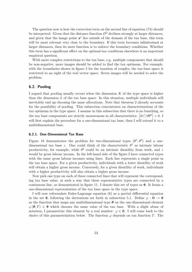
The question now is how the correction term on the second line of equation (74) shouldbe interpreted. Given that the distance function D2 declines strongly at larger distances,and given that the image point xi lies outside of the domain of the tax base, this termwill be most relevant very close to the boundary. If this term becomes infinitesimal atlarger distances, then its mere function is to enforce the boundary conditions. Whetherthis term has a significant effect on the optimal-tax conditions elsewhere is an importantempirical question.
With more complex restrictions to the tax base, e.g. multiple components that shouldbe non-negative, more images should be added to find the tax optimum. For example,with the boundaries shown in figure 5 for the taxation of couples, the tax-base space isrestricted to an eight of the real vector space. Seven images will be needed to solve theproblem.
6.2. PoolingI argued that pooling usually occurs when the dimension K of the type space is higherthan the dimension L of the tax base space. In this situation, multiple individuals willinevitably end up choosing the same allocations. Note that theorem 2 already accountsfor the possibility of pooling. This subsection concentrates on characterizations of thetax optimum in the type space. I assume in this subsection that there is no bunching, sothe tax base components are strictly monotonous in all characteristics:
∣∣∣∂zl/∂θk∣∣∣ > 0. Iwill first explain the procedure for a one-dimensional tax base, then I will extend it to amultidimensional base.
6.2.1. One-Dimensional Tax Base
Figure 10 demonstrates the problem for two-dimensional types(θ1, θ2) and a one-
dimensional tax base z. One could think of the characteristic θ1 as intrinsic labourproductivity, for example, while θ2 could be an intrinsic disutility from work, and zwould be gross labour income. In the left-hand side of the figure I have connected typeswith the same gross labour incomes using lines. Each line represents a single point inthe tax base space. For a given productivity, individuals with a lower disutility of workwill obtain a higher gross income. Conversely, for a given disutility of work, individualswith a higher productivity will also obtain a higher gross income.
Now pick one type on each of these connected lines that will represent the correspond-ing tax base value, in such a way that these representative types are connected by acontinuous line, as demonstrated in figure 11. I denote this set of types as Φ. It forms aone-dimensional representation of the tax base space in the type space.
I will now reformulate Euler-Lagrange equation (6) as a partial differential equationin the set Φ, following the derivations set forth in subsection 5.1. Define ϕ : Θ → Φas the function that maps any multidimensional type θ on the one-dimensional elementϕ (θ, T ) ∈ Φ which chooses the same value of the tax base. With a slight abuse ofnotation, I parametrize this element by a real number: ϕ ∈ R. I will come back to thechoice of this parametrization below. The function ϕ depends on tax function T . The
53

Figure 10: An example of pooling, with a two-dimensional type space and a one-dimensional tax base space. Each value z of the tax base corresponds toa one-dimensional set of types. For example, types a and b choose the samevalue z (a) = z (b) of the tax base, and types c and d choose the same valuez (c) = z (d). The one-dimensional subsets of the type space who choose thesame values of the tax base, are connected using lines.
θ1
θ2
z
a
b
c
d
z (a) = z (b) z (c) = z (d)
Figure 11: Since multiple types end up pooling at the same tax base values, we pick onetype to represent each tax base value, such that the one-dimensional set Φof these representative types forms a line in the type space. I parametrizethe coordinates on this line as a scalar ϕ. For each type θ ∈ Θ, the scalarfunction ϕ (θ, T ) then indicates which point in the set of representative typesΦ chooses the same value for the tax base.
θ1
θ2
Φ
ϕ (a ′) =ϕ (a ′′)
a′
a′′
b′
c′
b′′c′′
ϕ (c ′) =ϕ (c ′′)
ϕ (b ′ )
=ϕ (b ′′ )
54

reason is that different types who pool together at one level of the tax base in presenceof a given tax function, might choose different values of the tax base when another taxfunction is in place.
Denote the cumulative distribution function on the set Φ as F Φ (ϕ), with correspondingdensity function fΦ (ϕ). Define the function zΦ that maps any element in Φ on the taxbase value in X that it represents:
∀θ : zΦ (ϕ (θ, T ) , T ) ≡ z (θ, T ) .
The procedures set forth in subsection 5.1 then imply that Euler-Lagrange equation (6)can then be rewritten as follows:
∀θ : ∂∂ϕ
{[TzzTz ]
(zΦ (ϕ (θ, T ) , T )
)zΦϕ (ϕ (θ, T ) , T ) fΦ (ϕ (θ, T ))
}= [1− α (z (θ, T ))] fΦ (ϕ (θ, T )) .
The main difference with theorem 3, besides the dimensionality, is that the welfareweights α and the behavioural responses zTz are now averaged over the multitude ofindividuals pooling at the given value of the tax base.
Integrate the latter result and write the average behavioural response at z as anintegral over the type space:
∀θ : Tz (z (θ, T ))fΦ (ϕ (θ, T ))(∫Θ
zTz
(θ′)
zΦϕ (ϕ (θ, T ) , T )dFΘ|X(θ′|z (θ, T )
))(75)
= −∫ ∞ϕ(θ,T )
[1− α
(zΦ(ϕ′, T
))]fΦ(ϕ′)
dϕ′.
The interpretation of this result is similar to the interpretation of equation (51) in section5. The right-hand side represents the distributional advantage of taxation, the left-handside represents the cost of redistribution.
One question now is how the function ϕ (θ, T ) should be parametrized. The poolingfunctions introduced by Jacquet and Lehmann (2016) are one possibility.28 If preferencesare separable between consumption and leisure, equation (75) corresponds to the resultfound by Jacquet and Lehmann (2016) in their proposition 1.
A different possibility is to simply parametrize ϕ (θ, T ) by the gross tax income that itrepresents. Substituting z for ϕ in equation (75) recovers optimal-tax equation (7) in thetax base space. It is not clear at this point why one parametrization should be preferredover the other. Different parametrizations might lead to different insights, dependingon the problem being studied. The question of the optimal parametrization remains atopic for further research.28Jacquet and Lehmann (2016) divide the type vector into a one-dimensional wage, and a vector of
other characteristics. They choose a reference value of these other characteristics. Keeping constantthese other characteristics at the reference value, and varying the wage, they trace out a straight,one-dimensional path in the type space. Assuming that different wages yield different gross labourincomes, this one-dimensional path is a representation of the gross incomes. In terms of my approach,the value of the wage is then used as a parametrization of the different points on this line.
55

We can further reinterpret equation (75), using similar derivations as those in subsec-tion 5.1. Use the implicit function theorem to find:
∀θ : Tz (z (θ, T )) dϕ
dTz
∣∣∣∣∣z(θ,T )
= 1fΦ (ϕ)
∫ ∞ϕ(θ,T )
[1− α
(zΦ(ϕ′, T
))]fΦ(ϕ′)
dϕ′, (76)
where I rewrite the integral on the left-hand side as an average at z (θ, T ). This ex-pression can again be interpreted as an information cost, similar to what we found insubsection 5.1. Individuals who originally pool at z (θ, T ) are represented by the sametype ϕ (θ, T ). If there is a tax reform, these individuals will respond, and they willbecome represented by a different type in Φ. The derivative on the left-hand side ofequation (76) denotes the average of these responses. The larger are these responses,the more difficult it will be to target specific types, and the lower will be the optimalmarginal tax rate.
Similarly, using methods and notations from subsection 5.2, we can reformulate equa-tion (75) as follows:
∀θ : Tz (z (θ, T )) = 1fΦ (ϕ)
∂ (uz/uc)∂ϕ
∣∣∣∣∣z(θ,T )
{∫ ∞ϕ(θ,T )
[1− α
(zΦ(ϕ′, T
))]fΦ(ϕ′)
dϕ′}.
Again the term ∂ (uz/uc) /∂ϕ∣∣∣z
is an indication of how able the government is to targetspecific types. If a characteristic has a large effect on the marginal rate of substitution,then the government can use small changes in the marginal tax rate to precisely targetthe individuals it would like to target.
6.2.2. Multidimensional Tax Base
We now have the necessary tools to study the phenomenon of pooling with a multidi-mensional tax base. Still assuming that the type space Θ has a higher dimension thanthe tax base space X , K > L, the subsets of Θ that connect types who pool at thesame tax base value will have dimension K − L. For example, with four-dimensionaltypes and a two-dimensional tax base, each point of the two-dimensional tax base wouldcorrespond to a two-dimensional plane in the four-dimensional type space.
Figure 12 demonstrates the situation for a two-dimensional tax base and a three-dimensional type space, where again types sharing the same value of the tax base formone-dimensional sets. The set Φ representing the tax base space in the type space is atwo-dimensional plane. The derivations below are valid for any combination K > L.Denote the cumulative distribution function on the set Φ as F Φ (ϕ), with correspondingdensity function fΦ (ϕ).
Define ϕ : Θ → Φ as the vector-valued function that maps any K-dimensional type θon the L-dimensional element ϕ (θ) ∈ Φ, which is parametrized as a real vector (ϕ ∈ RL).Introduce the function xΦ : Φ → X which maps any element ϕ ∈ Φ on the tax basevalue x ∈ X that it represents:
∀θ : xΦ (ϕ (θ, T ) , T ) ≡ x (θ, T ) .
56

Figure 12: With three-dimensional types and two-dimensional tax base values, there areone-dimensional sets in the type space who end up choosing the same valueof the tax base. On each of these lines we pick one type, which represents thecorresponding value of the tax base, such that the two-dimensional set Φ ofthese representative types forms a plane in the type space. The coordinateson this plane are parametrized by a vector ϕ. For each type θ ∈ Θ, thefunction ϕ (θ, T ) then indicates which point in the set of representative typesΦ chooses the same value for the tax base.
θ1
θ2
θ3
Φ
θ′
θ′′
ϕ (θ′, T )
ϕ (θ′′, T )
Introduce the Jacobian matrix for this function:
J Φ ≡
xΦ,1ϕ1 · · · xΦ,1
ϕL
... . . . ...xΦ,Lϕ1 · · · xΦ,L
ϕL
.Using again the derivations from subsection 5.1, we can now reformulate Euler-Lagrange
equation (12) in the representative space Φ:
∀θ ∈ Θ :(1− α
(xΦ (ϕ (θ, T ) , T )
))fΦ (ϕ (θ, T )) (77)
=L∑l=1
∂
∂ϕl
{[∇xT · x∇xT ·
[(J Φ
)−1]ᵀ]l (
xΦ (ϕ (θ, T ) , T ))fΦ (ϕ (θ, T ))
}.
The solution for this differential equation is entirely analogue to what we found in theprevious subsection:
∀θ :[∇xT · x∇xT ·
[(J Φ
)−1]ᵀ]
(x (θ, T ))
= 1fΦ (ϕ (θ, T ))cov
(α(xΦ(ϕ′, T
)),
ϕ′ −ϕDK (ϕ′ −ϕ)
).
We can rewrite the left-hand side using derivations analogue to those in the previous
57

subsection:
∀θ : ∇xT (x (θ, T )) · dϕ
d∇xT
∣∣∣∣∣ᵀ
x
= − 1fΦ (ϕ (θ, T ))cov
(α(xΦ(ϕ′, T
)),
ϕ′ −ϕDK (ϕ′ −ϕ)
),
or accounting for preference optimization:
∀θ : ∇xT (x (θ, T )) ·(∂ (ux/uc)
∂ϕ
∣∣∣∣−1
x
)ᵀ
= − 1fΦ (ϕ (θ, T ))cov
(α(xΦ(ϕ′, T
)),
ϕ′ −ϕDK (ϕ′ −ϕ)
).
The interpretation of these equations is fully analogue to those in the previous subsec-tions: the government balances the advantage of redistribution of increasing the marginaltax rate in a given direction, against the cost of targeting specific characteristics of theindividuals.
6.3. BunchingWhen individuals of consecutive types all choose the same level of the tax base, wesay that they are bunching on that point. A range of points in the type space will beallocated to a single mass point in the tax base space. Ebert (1992) shows that it ispossible to find combinations of social preferences, individual preferences and populationdensities such that this situation occurs in the optimum.
Bunching can also occur on a higher-dimensional subset of the tax base space. Sayfor example that the tax base is two-dimensional, taxing capital income and labourincome. It is possible that different individuals with different capital incomes, all choosea corner solution where labour income is zero. The bunching range in this case is aone-dimensional line in the two-dimensional tax base space.
I show in subsection 6.3.1 how a bunching range in the interior of the tax base spacecan only be implemented through a kink in the tax function, and how this should betaken into account in the Euler-Lagrange formalism. In subsection 6.3.2 I show howtransversality condition (43) continues to apply in this situation. I show how the taxoptimum can then be characterized in presence of bunching in subsection 6.3.3. Finallyin subsection 6.3.4, I treat the possibility of bunching on an edge of the tax base space.
6.3.1. Validity of Euler-Lagrange Equation
Suppose that there is a one-dimensional type θ, a one-dimensional tax base x, and anumeraire commodity c. Suppose that individuals optimize a utility function u (c, x, θ),subject to the budget constraint c = x−T (x). If the tax function is differentiable, thenthe first-order condition for the individual is as follows:
uxuc
= −(1− T ′ (x)
). (78)
58

Figure 13: Bunching at tax base value X. The tax function T (x) has a kink at X,causing individuals of different types θ′ and θ′′, with indifference curves ofdifferent slopes, to choose the same value of the tax base.
xX
x− T(x)
IC(θ′)
IC(θ′′)
c
Assume that the following single-crossing condition is fulfilled:
∂ (ux/uc)∂θ
> 0. (79)
Mirrlees (1976) then shows that the second-order condition for the individual optimiza-tion problem is equivalent to the following weak monotonicity condition:
dx
dθ≥ 0.
Ebert (1992) shows that it is possible to find combinations of social preferences, in-dividual preferences and population densities such that the second-order condition isbinding on some range of the type space: dx/dθ = 0. It immediately follows from con-ditions (78) and (79) that this allocation cannot be implemented using a smooth taxfunction. In order to implement it, there needs to be a kink in the tax function. Figure13 shows how this works: both types θ′ and θ′′, with indifference curves of differentslopes, choose the same value X of the tax base. The problem with a kink in the taxfunction is that the Euler-Lagrange equation (12) in theorem 1 is no longer well-defined:the marginal tax rate Tx is not defined in the bunching point.
It is straightforward to see though that outside of the bunching point, the tax reformsconstructed in subsection 3.1 should still leave social welfare unchanged. It followsthat Euler-Lagrange equation (6) remains valid everywhere, except at the kink in thetax function. This reasoning is straightforward to extend to higher dimensions: Euler-Lagrange equation (12) remains valid outside of the bunching ranges.
59
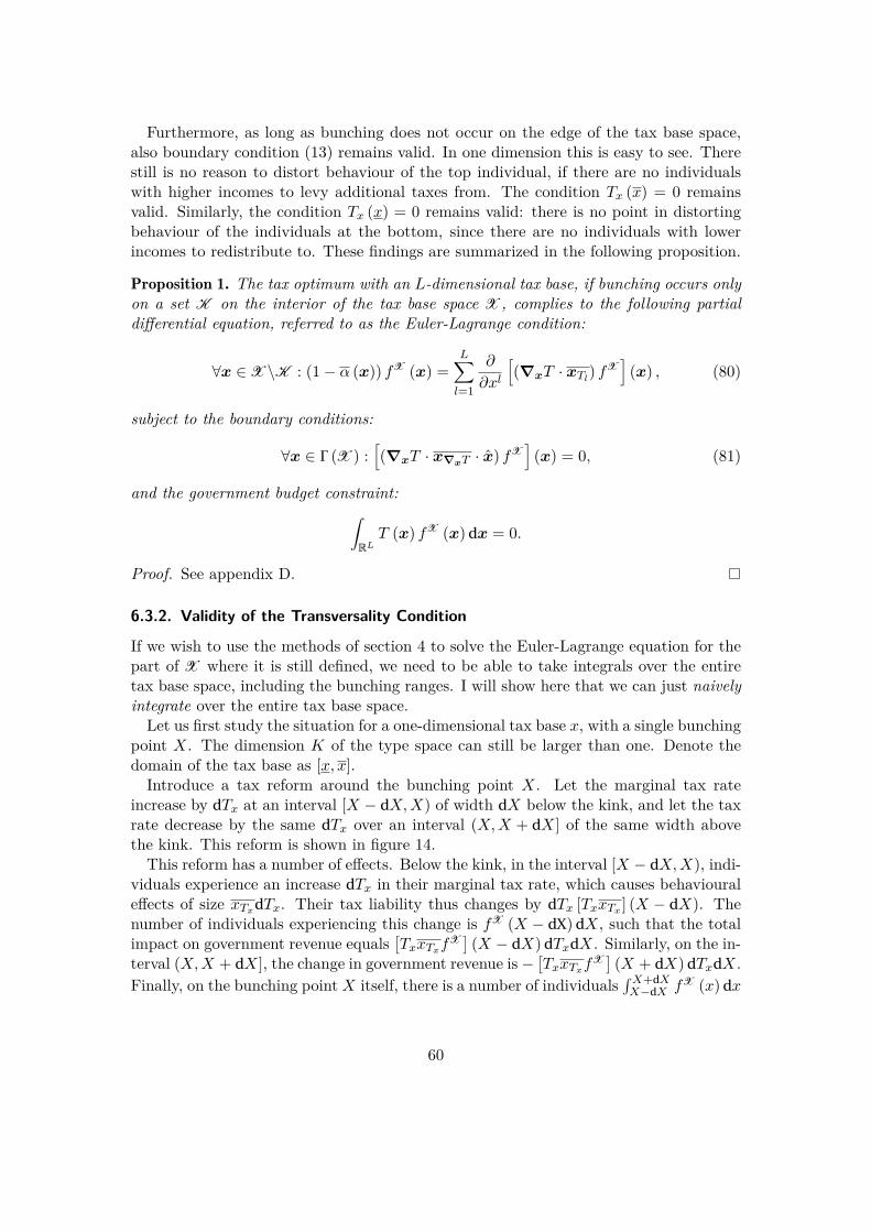
Furthermore, as long as bunching does not occur on the edge of the tax base space,also boundary condition (13) remains valid. In one dimension this is easy to see. Therestill is no reason to distort behaviour of the top individual, if there are no individualswith higher incomes to levy additional taxes from. The condition Tx (x) = 0 remainsvalid. Similarly, the condition Tx (x) = 0 remains valid: there is no point in distortingbehaviour of the individuals at the bottom, since there are no individuals with lowerincomes to redistribute to. These findings are summarized in the following proposition.
Proposition 1. The tax optimum with an L-dimensional tax base, if bunching occurs onlyon a set K on the interior of the tax base space X , complies to the following partialdifferential equation, referred to as the Euler-Lagrange condition:
∀x ∈ X \K : (1− α (x)) fX (x) =L∑l=1
∂
∂xl
[(∇xT · xTl
) fX]
(x) , (80)
subject to the boundary conditions:
∀x ∈ Γ (X ) :[(∇xT · x∇xT · x) fX
](x) = 0, (81)
and the government budget constraint:∫RLT (x) fX (x) dx = 0.
Proof. See appendix D.
6.3.2. Validity of the Transversality Condition
If we wish to use the methods of section 4 to solve the Euler-Lagrange equation for thepart of X where it is still defined, we need to be able to take integrals over the entiretax base space, including the bunching ranges. I will show here that we can just naivelyintegrate over the entire tax base space.
Let us first study the situation for a one-dimensional tax base x, with a single bunchingpoint X. The dimension K of the type space can still be larger than one. Denote thedomain of the tax base as [x, x].
Introduce a tax reform around the bunching point X. Let the marginal tax rateincrease by dTx at an interval [X − dX,X) of width dX below the kink, and let the taxrate decrease by the same dTx over an interval (X,X + dX] of the same width abovethe kink. This reform is shown in figure 14.
This reform has a number of effects. Below the kink, in the interval [X − dX,X), indi-viduals experience an increase dTx in their marginal tax rate, which causes behaviouraleffects of size xTx dTx. Their tax liability thus changes by dTx [TxxTx ] (X − dX). Thenumber of individuals experiencing this change is fX (X − dX) dX, such that the totalimpact on government revenue equals
[TxxTxf
X ] (X − dX) dTxdX. Similarly, on the in-terval (X,X + dX], the change in government revenue is −
[TxxTxf
X ] (X + dX) dTxdX.Finally, on the bunching point X itself, there is a number of individuals
∫X+dXX−dX fX (x) dx
60

Figure 14: The size of the tax reform around the bunching point X. The marginal taxrate is increased by dTx over the interval [X − dX,X), and it is decreasedagain by dTx over the interval (X,X + dX]. BelowX−dX and aboveX+dX,the tax liability remains unaltered. The change in the tax liability at X equalsdXdTx.
X − dX xX
dTx
dT (x)
dXdTx−dTx
X + dX
who experience an increase dXdTx in their tax liability.29 The effect on social welfareequals dTxdX
∫X+dXX−dX (1− α (x)) fX (x) dx. Sum all these effects, divide by dTxdX and
require that the result is zero:[TxxTxf
X]
(X + dX)−[TxxTxf
X]
(X − dX) =∫ X+dX
X−dX(1− α (x)) fX (x) dx. (82)
Since the derivative of the tax function at X is not defined, we can no longer obtain thetraditional Euler-Lagrange equation from this condition.
What we are interested in now is how to calculate the integral of the entity (1− α (x)) fX (x)from a value of the tax base x′ below the kink, to a value x′′ above the kink. Note firstwhat happens if we integrate on the part below the kink:∫ X−dX
x′(1− α (x)) fX (x) dx =
∫ X−dX
x′
d
dx
[TxxTxf
X]
(x) dx
=[TxxTxf
X]
(X − dX)−[TxxTxf
X] (x′),
where I use the validity of the Euler-Lagrange equation on this range (by proposition1). Similarly, above the kink:∫ x′′
X+dX(1− α (x)) fX (x) dx =
∫ x′′
X+dX
d
dx
[TxxTxf
X]
(x) dx
=[TxxTxf
X] (x′′)−[TxxTxf
X]
(X + dX) .
Adding the last two equations and using result (82), taking the limit dX → 0:
limdX→0
[∫ X−dX
x′(1− α (x)) fX (x) dx+
∫ x′′
X+dX(1− α (x)) fX (x) dx
]
= − limdX→0
[∫ X+dX
X−dX(1− α (x)) fX (x) dx
]+[TxxTxf
X] (x′′)−[TxxTxf
X] (x′).
29Note that the imprecisions in this derivation disappear as dX → 0. These results follow more formallyfrom equation (104) in appendix D.
61
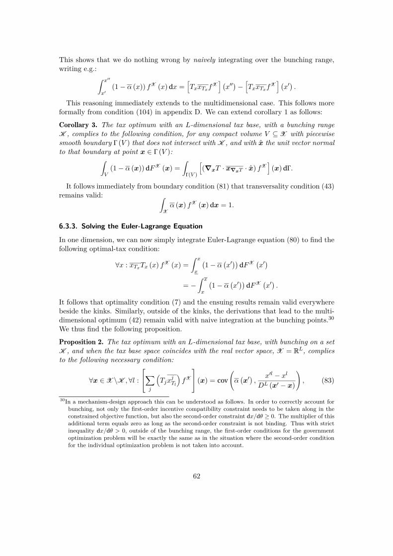
This shows that we do nothing wrong by naively integrating over the bunching range,writing e.g.:∫ x′′
x′(1− α (x)) fX (x) dx =
[TxxTxf
X] (x′′)−[TxxTxf
X] (x′).
This reasoning immediately extends to the multidimensional case. This follows moreformally from condition (104) in appendix D. We can extend corollary 1 as follows:
Corollary 3. The tax optimum with an L-dimensional tax base, with a bunching rangeK , complies to the following condition, for any compact volume V ⊆ X with piecewisesmooth boundary Γ (V ) that does not intersect with K , and with x the unit vector normalto that boundary at point x ∈ Γ (V ):∫
V(1− α (x)) dFX (x) =
∫Γ (V )
[(∇xT · x∇xT · x) fX
](x) dΓ .
It follows immediately from boundary condition (81) that transversality condition (43)remains valid: ∫
Xα (x) fX (x) dx = 1.
6.3.3. Solving the Euler-Lagrange Equation
In one dimension, we can now simply integrate Euler-Lagrange equation (80) to find thefollowing optimal-tax condition:
∀x : xTxTx (x) fX (x) =∫ x
x
(1− α
(x′))
dFX(x′)
= −∫ x
x
(1− α
(x′))
dFX(x′).
It follows that optimality condition (7) and the ensuing results remain valid everywherebeside the kinks. Similarly, outside of the kinks, the derivations that lead to the multi-dimensional optimum (42) remain valid with naive integration at the bunching points.30
We thus find the following proposition.
Proposition 2. The tax optimum with an L-dimensional tax base, with bunching on a setK , and when the tax base space coincides with the real vector space, X = RL, compliesto the following necessary condition:
∀x ∈ X \K ,∀l :
∑j
(Tjx
jTl
)fX
(x) = cov
(α(x′),
x′l − xl
DL (x′ − x)
), (83)
30In a mechanism-design approach this can be understood as follows. In order to correctly account forbunching, not only the first-order incentive compatibility constraint needs to be taken along in theconstrained objective function, but also the second-order constraint dx/dθ ≥ 0. The multiplier of thisadditional term equals zero as long as the second-order constraint is not binding. Thus with strictinequality dx/dθ > 0, outside of the bunching range, the first-order conditions for the governmentoptimization problem will be exactly the same as in the situation where the second-order conditionfor the individual optimization problem is not taken into account.
62
with transversality condition: ∫RLα (x) fX (x) dx = 1. (84)
Remember that without bunching points, the optimal tax function is pinned downwhen the Euler-Lagrange equation is given, together with the transversality conditionand the government budget constraint. If the Euler-Lagrange equation is no longer validin a bunching point, this creates a degree of indeterminacy in the problem. Even if themarginal tax rates comply to the Euler-Lagrange equation in all other points, it is notclear what happens in the kink. Since in this paper I have always assumed that thepermissible tax reforms are continuous functions, I assume here that the tax function iscontinuous in the kink. This assumption suffices to solve the indeterminacy.
6.3.4. Bunching on the Edge
A special case occurs when individuals bunch on an edge of the tax-base space. Takefor example the situation of figure 9, where the tax base consists of labour income z andcapital income y, so x ≡ (z, y), with the value of z restricted to be positive. If thereis bunching on the edge, so a mass of individuals chooses a corner solution at z = 0,this does not change the form of the optimal-tax equation at the interior of the tax basespace. The method of images can be applied, and equation (74) remains valid.
Without bunching at the bottom, we know that the boundary condition at z = 0would be that total tax wedge caused by the tax on labour income, TzzTz +TyyTz , equalszero. This changes when there is bunching at z = 0. To see this, imagine that there is anincrease dT in the tax liability for all individuals who have labour income z = 0, whichphases out over the infinitesimal interval z = [0,dZ]. The effect on social welfare of theincreased tax liability equals dT
∫ dZ0∫+∞−∞ (1− α (z′, y′)) fX (z′, y′) dy′dz′, while the ensu-
ing change in the marginal tax rate has an effect dT∫+∞−∞ (TzzTz + TyyTz ) fX (dz, y′) dy′
on government revenue. Demanding that the total effect of this reform sums to zero andtaking the limit dz → 0 yields:31
limdz→0
∫ dZ
0
∫ +∞
−∞
(1− α
(z′, y′
))fX
(z′, y′
)dy′dz′
= − limdz→0
∫ +∞
−∞(TzzTz + TyyTz ) fX
(dz, y′
)dy′.
The left-hand side of this equation would go to zero in the case without bunching atz = 0. If there is a mass of individuals bunching in this corner though, this is no longerthe case. It follows that the total tax wedge for the workers with the lowest non-zeroincome no longer converges to zero. Assuming that welfare weights are larger than oneat the bottom, we find TzzTz + TyyTz > 0 at the bottom. This extends the findings ofSeade (1977) to multiple dimensions.31A more formal derivation would be analogue to that of condition (104) in appendix D.
63

Figure 15: The type space Θ has only one dimension, while the tax base space Xhas two dimensions. The allocation, mapping types θ on tax base values(x1 (θ) , x2 (θ)
), forms a line, i.e. a one-dimensional subset of X .
x1
x2θ
θ
x(θ)
x (θ)
θ′
θ′′
x (θ′)
x (θ′′)
Θ
X
6.4. Lower-Dimensional AllocationsWhen the type space has a lower dimensionality than the tax base space, K < L, thenthe optimal allocation in the tax base space will also be K-dimensional, and as such itwill not be surjective on the real vector space RL. Even if individuals are free to chooseany bundle in RL, the government’s objective (1) is an integral over all types in thepopulation, and thus, after changing variables, over the actually chosen bundles in thetax base space. Since the domain of the optimization is no longer the entire real vectorspace RL, the optimal-tax condition in theorem 2 is no longer valid. The trick to findinga necessary condition for the tax optimum is again to find a suitable Green function.
Assume thus that we observe a tax function T , defined on an L-dimensional tax basespace X . We observe an income distribution which is restricted to a one-dimensionalset, a line within X which is the image of a one-dimensional type space Θ. We alsoobserve marginal behavioural responses x∇T everywhere on this line. Denote the one-dimensional types as θ, with corresponding tax base values x (θ, T ). Denote the bound-ary values of the type space as
[θ, θ]. This situation is illustrated for a two-dimensional
tax base in figure 15.The Green function for this problem is the vector-valued mapping defined by the
following equation:
∀x,x′, l : Gl(x,x′
)≡ δ
(x1 − x′1
). . . δ
(xl−1 − x′l−1
)·H
(xl − x′l
L
)δ(xl+1 − x′l+1
). . . δ
(xL − x′L
),
with H the unit step function defined in equation (22), and δ the Dirac delta function.To see that this is indeed the Green function for our problem, note first that condition
64

(31) is fulfilled:
∀x,x′ :∑l
∂Gl (x,x′)∂xl
= δL(x− x′
),
where I use definition (29) for the multidimensional Dirac delta function and property(23) of the unit step function. Second, note that G becomes zero at the edges, becauseof the unit step function H in its definition:
∀x′, l : Gl(x (θ) ,x′
)= Gl
(x(θ),x′)
= 0.
Now that we found the Green function for this optimal-tax problem, we can substi-tute it into equation (33). Use property (18) of the Dirac delta function to reduce themultidimensional integral to a one-dimensional integral over xl, and find the followingnecessary optimal-tax condition:
∀x, l :∑j
TjXjTl
=∫ xl
xl(1− α) dF l
(x′l),
with F l the cumulative density function for tax base component xl, and Xj aggregatedemand for component xj . Note that if xl is monotonous, ∂xl/∂θ > 0, then the integralon the right-hand side is the same for all components of the tax base. What follows isa traditional Ramsey-style proportional-reduction equation:
∀θ :∑j
TjXjT1
(θ) = . . . =∑j
TjXjTL
(θ) =∫ θ
θ(1− α) dFΘ
(θ′),
which corresponds to the solution traditionally found in the literature (see e.g. Jacobsand Boadway, 2014). Note that the optimal tax function in this case is separable,confirming the findings of Renes and Zoutman (2016b).
7. ConclusionI introduced the Euler-Lagrange method to characterize the optimum for problems withmultidimensional tax bases and multiple dimensions of heterogeneity of the agents. Ishowed the general applicability of the Euler-Lagrange equation as a first-order condition.I introduced the localized distributional characteristic, and I used it to provide a numberof characterizations for the optimum, both in terms of sufficient statistics and of economicfundamentals. I applied my findings to the Diamond and Spinnewijn (2011) optimalmixed labour and capital income tax problem and to the problem of the optimal jointtaxation of households as described by Kleven, Kreiner, and Saez (2007). Finally, Ishowed that the method is robust to a number of potential complications.
A drawback of this paper, that is not easily solved using the formalism at hand, isthat all responses to tax reform are assumed to be local. However, this is not uncommonin the literature, it is even generally assumed in most papers referred to in the present
65
publication. Still it would be interesting to allow for a participation margin – as inJacquet, Lehmann, and Van der Linden (2013) – or for more general discrete jumps– e.g. allowing for a discrete-choice behavioural model. There is also potential forextensions towards different objective functions, taking into account different normativeconvictions, political-economy considerations, or alternative behavioural models.
8. AcknowledgementsThis paper is part of the dissertation of the author to obtain the degree of Doctor inEconomics. I am most grateful to my supervisor Andre Decoster, and to the members ofmy commission: Robin Boadway, Bas Jacobs, Laurence Jacquet, Erik Schokkaert, FransSpinnewijn and Jo Van Biesebroeck. This paper has benefited from useful discussionswith Geert Dhaene, Aart Gerritsen, Etienne Lehmann, Saso Polanec and Floris Zout-man.I acknowledge the financial support of the Belgian Federal Science Policy Office (BEL-SPO) via the BRAIN.be project BR/121/A5/CRESUS, and of the Flemish ResearchFoundation (FWO) via travel grant V464515N.
ReferencesArfken, George B and Hans J Weber. 2005. Mathematical methods for physicists inter-
national student edition. Academic press.
Armstrong, Mark. 1996. “Multiproduct nonlinear pricing.” Econometrica: Journal ofthe Econometric Society :51–75.
Atkinson, A.B. and J.E. Stiglitz. 1980. Lectures on public economics. McGraw-HillCollege.
Atkinson, Anthony B and Joseph E Stiglitz. 2015. Lectures on public economics. Prince-ton University Press.
Atkinson, Anthony Barnes and Joseph E Stiglitz. 1976. “The design of tax structure:direct versus indirect taxation.” Journal of Public Economics 6 (1-2):55–75.
Boadway, Robin. 2012. From optimal tax theory to tax policy. Munich Lectures inEconomics. The MIT Press.
Bohacek, Radim and Michal Kejak. 2016. “Optimal Government Policies in Models withHeterogeneous Agents.” .
Christiansen, Vidar. 1984. “Which commodity taxes should supplement the incometax?” Journal of public economics 24 (2):195–220.
Christiansen, Vidar and Matti Tuomala. 2008. “On taxing capital income with incomeshifting.” International Tax and Public Finance 15 (4):527–545.
66
Corlett, W.J. and D.C. Hague. 1953. “Complementarity and the excess burden of taxa-tion.” The Review of Economic Studies 21 (1):21–30.
Courant, R and D Hilbert. 1953. “Methods of Mathematical Physics Vol. I. Translatedand revised from the German original. First English ed.”
Cremer, H., P. Pestieau, and J.C. Rochet. 2001. “Direct versus indirect taxation: thedesign of the tax structure revisited.” International Economic Review 42 (3):781–800.
Diamond, Peter and Johannes Spinnewijn. 2011. “Capital income taxes with heteroge-neous discount rates.” American Economic Journal: Economic Policy 3 (4):52–76.
Diamond, Peter A. 1975. “A many-person Ramsey tax rule.” Journal of Public Eco-nomics 4 (4):335–342.
———. 1998. “Optimal income taxation: an example with a U-shaped pattern of optimalmarginal tax rates.” American Economic Review :83–95.
Ebert, Udo. 1992. “A Reexamination of the Optimal Nonlinear Income Tax.” Journalof Public Economics 49 (1):47–73.
Feldstein, Martin S. 1972a. “Distributional equity and the optimal structure of publicprices.” The American Economic Review 62 (1/2):32–36.
———. 1972b. “Equity and efficiency in public sector pricing: the optimal two-parttariff.” The Quarterly Journal of Economics :176–187.
Gerritsen, Aart. 2016. “Optimal nonlinear taxation: the dual approach.”
Gerritsen, Aart, Bas Jacobs, Alexandra Rusu, and Kevin Spiritus. 2015. “OptimalTaxation of Capital Income when Individuals have Different Returns.” Mimeo, MaxPlanck Institute Munich/Erasmus University Rotterdam/KU Leuven.
Jacobs, Bas. 2013. “The marginal cost of public funds is one at the optimal tax system.”Erasmus University Rotterdam .
Jacobs, Bas and Robin Boadway. 2014. “Optimal linear commodity taxation underoptimal non-linear income taxation.” Journal of Public Economics 117:201–210.
Jacquet, Laurence and Etienne Lehmann. 2016. “Optimal Taxation with HeterogeneousSkills and Elasticities: Structural and Sufficient Statistics Approaches.”
Jacquet, Laurence, Etienne Lehmann, and Bruno Van der Linden. 2013. “Optimal redis-tributive taxation with both extensive and intensive responses.” Journal of EconomicTheory 148 (5):1770–1805.
Kleven, Henrik Jacobsen, Claus Thustrup Kreiner, and Emmanuel Saez. 2007. “Theoptimal income taxation of couples as a multi-dimensional screening problem.” (2092).
67

Lax, Peter D, Michael E Taylor, Michael E Taylor, and Michael E Taylor. 1998. “PartialDifferential Equations I: Basic Theory.”
Mirrlees, J.A. 1971. “An exploration in the theory of optimum income taxation.” Thereview of economic studies 38 (2):175–208.
———. 1976. “Optimal tax theory: A synthesis.” Journal of Public Economics 6 (4):327–358.
Renes, Sander and Floris T Zoutman. 2016a. “As Easy as ABC? Multi-DimensionalScreening in Public Finance.” Mimeo, Erasmus Universiteit Rotterdam/NorwegianSchool of Economics.
———. 2016b. “When a Price is Enough.” .
Rochet, Jean-Charles. 1985. “The taxation principle and multi-time Hamilton-Jacobiequations.” Journal of Mathematical Economics 14 (2):113–128.
Rochet, Jean-Charles and Philippe Chone. 1998. “Ironing, sweeping, and multidimen-sional screening.” Econometrica :783–826.
Sadka, Efraim. 1976. “On Income Distribution, Incentive Effects and Optimal IncomeTaxation.” Review of Economic Studies 43 (2):261–267.
Saez, Emmanuel. 2001. “Using Elasticities to Derive Optimal Income Tax Rates.” Reviewof Economic Studies 68 (1):205–29.
———. 2002. “The desirability of commodity taxation under non-linear income taxationand heterogeneous tastes.” Journal of Public Economics 83 (2):217–230.
Saez, Emmanuel and Stefanie Stantcheva. 2016. “Generalized social marginal welfareweights for optimal tax theory.” The American Economic Review 106 (1):24–45.
Scheuer, Florian and Ivan Werning. 2016. “Mirrlees meets Diamond-Mirrlees.” Tech.rep., National Bureau of Economic Research.
Seade, Jesus K. 1977. “On the Shape of Optimal Tax Schedules.” Journal of PublicEconomics 7 (2):203–235.
Werquin, Nicolas, Aleh Tsyvinski, and Mikhail Golosov. 2015. “A Variational Approachto the Analysis of Tax Systems.” Tech. rep., Society for Economic Dynamics.
A. Proof for the Euler-Lagrange Equation in Theorem 1The derivations in this section extend the proof for the traditional Euler-Lagrange equa-tion, formulated in standard texts on the calculus of variations (see e.g. Arfken and
68

Weber, 2005, chapter 17). I extend it to our context with private information about theindividual types.
We are maximizing social welfare (1) subject to government budget constraint (2).If the tax function T is to be optimal, any small perturbation to it should leave socialwelfare unchanged. We are thus interested in the effects of perturbations of T .
For each value of the tax base x, introduce a reform of size εη (x). Here ε is asmall parameter that allows varying the size of the reform, and η (x) is an arbitrary,nonlinear but smooth tax reform function. The tax gradient at each point thus changesby ε∇xη (x).
For a given tax function T , I will seek the optimal value of the reform parameter εthat optimizes social welfare. If the tax function T is optimal, then the optimal value ofε will be zero for any function η.
I have assumed that when there is a marginal tax reform, the wellbeing of an individualis affected only by the change in the tax liability at the value of the tax base that hechose before the reform. Similarly, I have assumed that behaviour is affected only bythe changes in the tax liability and the tax gradient at the original value of the tax base.Taking into account the reform, the constrained objective function for the governmentis as follows:
L (ε) ≡∫Θ
[v (θ, T + εη (x))] dFΘ (θ) (85)
+ λ
∫Θ
[T (x+ xT εη (x) + x∇T · (ε∇xη (x))ᵀ) + εη (x)] dFΘ (θ) .
For the tax function T (·) to be optimal, it is necessary that the effect of a marginalchange to the parameter ε, evaluated in ε = 0, is zero for any reform function η (x):
0 = dL ε
dε
∣∣∣∣ε=0
=∫Θ
{(1 + vT
λ+ ∇xT · xT
)η (x)
}dFΘ (θ) (86)
+∫Θ{∇xT · x∇T · (∇xη (x))ᵀ}dFΘ (θ) .
I will now change variables in the integral. The law of iterated expectations tells usthat for any function g : Θ → RD, with D some dimensionality, a total expectation canbe rewritten as a total expectation over conditional expectations:∫
Θg (θ) dFΘ (θ) =
∫Θ
∫Θg (θ) dFΘ|X
(θ|x
(θ′, T
))dFΘ
(θ′), (87)
where I introduce the conditional cumulative density function FΘ|X (θ|x).The law of the unconscious statistician guarantees that a change of variables from
the type space to the tax-base space is possible in the outer integral without worryingabout the form of x (θ, T ), as long as the distribution function FΘ (θ) is replaced by thedistribution function FX (x). This allows rewriting condition (86):
0 =∫X
∫Θ
{(1 + vT
λ+ ∇xT · xT
)η (x)
}dFΘ|X (θ|x) dFX (x) (88)
+∫X
∫Θ{∇xT · x∇T · (∇xη (x))ᵀ}dFΘ|X (θ|x) dFX (x) .
69

Use integration by parts to rewrite the second term on the right:∫X
∫Θ{∇xT · x∇T · (∇xη (x))ᵀ}dFΘ|X (θ|x) dFX (x) (89)
=∫Γ (X )
∫Θ
{∇xT · x∇T · xfX (x)
}η (x) dFΘ|X (θ|x) dΓ
−∫X
∫Θ
∑l
∂
∂xl
{∇xT · xTl
fX (x)}η (x) dFΘ|X (θ|x) dx.
Substitute this into (88):
0 =∫X
∫Θ
{(1 + vT
λ+ ∇xT · xT
)fX (x) (90)
−∑l
∂
∂xl
{∇xT · xTl
fX (x)}}
dFΘ|X (θ|x) η (x) dx
+∫Γ (X )
∫Θ{∇xT · x∇T · x}dFΘ|X (θ|x) fX (x) η (x) dΓ .
The fundamental lemma of the calculus of variations states that this expression canonly be zero for all functions η if the integrands between curly brackets are zero for alltax-base levels x.
B. Two-Dimensional Green FunctionsSuppose x 6= x′. We find partial derivatives (using the fact that the surface area of acircle with radius r equals V 2 (r) = πr2):
∀x 6= x′, ∀l : ∂Gl (x,x′)∂xl
= 12π ||x− x′||2
+ xl − x′l
2π∂
∂ ||x− x′||
(1
||x− x′||2
)∂ ||x− x′||
∂xl
= 12π ||x− x′||2
− xl − x′l
π
1||x− x′||3
∂√
(x1 − x1′)2 + (x2 − x2′)2
∂xl
= 12π ||x− x′||2
−
(xl − xl′
)2
π ||x− x′||4. (91)
Sum these components over l to find property (35).Define S2 (x′, R) as the area enclosed by the circle around the point x′ with finite ra-
dius R. Since the partial derivative ∂Gl (x,x′) /∂xl is zero everywhere outside the pointx′, the following integral over the entire real space equals the integral over S2 (x′, R):
∫R2
( 2∑l=1
∂Gl (x,x′)∂xl
)dx =
∫S2(x′,R)
( 2∑l=1
∂Gl (x,x′)∂xl
)dx. (92)
70

Using the divergence theorem, we can rewrite the right-hand side of this equation asfollows: ∫
R2
( 2∑l=1
∂Gl (x,x′)∂xl
)dx =
∫Γ (S2(x′,R))
x− x′
2V 2 (||x− x′||) · xdΓ , (93)
where I substitute formulation (34) for the Green function G. Note that everywhereon the boundary Γ
(S2 (x′, R)
), we have ||x− x′|| = R, so we can move the term
V 2 (||x− x′||) out of the integral:∫R2
( 2∑l=1
∂Gl (x,x′)∂xl
)dx = 1
2V 2 (R)
∫Γ (S2(x′,R))
(x− x′
)· xdΓ . (94)
Again using the divergence theorem on the right-hand side:
∫R2
( 2∑l=1
∂Gl (x,x′)∂xl
)dx = 1
2V 2 (R)
∫S2(x′,R)
2∑l=1
∂(xl − x′l
)∂xl
dx (95)
=2∫S2(x′,R) dx
2V 2 (R) .
Since∫S2(x′,R) dx equals the area of any circle with radius R, this proves property (36).
This reasoning extends to any dimensionality L ≥ 2, leading to the results of subsec-tion 4.3. The Green function generally takes the following form:
G(x,x′
)≡ x− x′
LV L (||x− x′||) ,
which solves the following partial differential equation:
∀x ∈ RL : δL(x− x′
)=
L∑l=1
∂Gl (x,x′)∂xl
, (96)
complying to the following boundary condition:
∀x ∈ Γ (X ) ,∀x′ ∈ X : G(x,x′
)· x = 0. (97)
Adding any divergence-free vector field to G also solves the problem, since this leavesthe divergence of G unaltered. Partial differential equation (96) thus has many solu-tions. For our specific problem, the above formulation is the one that we are interestedin. To see this, note that the vector field B in equation (26) is conservative, being agradient of the government budget constraint. We are thus interested in irrotationalGreen functions. Suppose now that two different irrotational functions solve divergenceequation (96) subject to boundary condition (97). The difference between these twofunctions has divergence zero. Since it is also irrotational, it is a harmonic function.Since it disappears at the boundary, because of condition (97), it is zero everywhere. Itfollows that if two irrotational functions solve partial differential equation (96) subjectto condition (97), they are necessarily equal.
71

C. Euler-Lagrange Equation in Type SpaceStart from equation (86). Use the chain rule to find the following relation:
∇xη (x) = ∇θη (x) ·J −1. (98)
Substitute this into equation (86):
0 = dL ε
dε
∣∣∣∣ε=0
=∫Θ
(1− α) η (x) dFΘ (θ) (99)
+∫Θ
{∇xT · x∇T ·
(J −1
)ᵀ· (∇θη (x))ᵀ
}dFΘ (θ) .
Use integration by parts to rewrite the right-hand side:∫Θ
{∇xT · x∇T ·
(J −1
)ᵀ· (∇θη (x))ᵀ
}dFΘ (θ) (100)
=∫Γ (Θ)
{∇xT · x∇T ·
(J −1
)ᵀ· θ}η (x) fΘ (θ) dθ
−∫Θ
∑k
∂
∂θk
{∇xT · x∇T ·
(J −1
)ᵀfΘ (θ)
}η (x) d (θ) .
Substitute this into (99):
0 =∫Θ
{(1− α) fΘ (θ)−
∑k
∂
∂θk
(∇xT · x∇T ·
(J −1
)ᵀfΘ (θ)
)}η (x) dθ (101)
+∫Γ (Θ)
{∇xT · x∇T ·
(J −1
)ᵀ· θ}η (x) fΘ (θ) dθ.
The fundamental lemma of the calculus of variations states that this expression can onlybe zero for all functions η if the integrands between curly brackets are zero for all typesθ.
D. Proof of Euler-Lagrange Equation with BunchingDenote as B ⊂ Θ the set of types who belong to a bunching range. I assume thatthere is only one such range, so the set B is connected. This proof readily extends toa situation with multiple bunching ranges. The tax gradient ∇xT is not defined on theset B .
Optimality condition (86) can be adapted to this situation:
0 = dL ε
dε
∣∣∣∣ε=0
=∫Θ\B
{(1 + vT
λ+ ∇xT · xT
)η (x)
}dFΘ (θ) (102)
+∫Θ\B{∇xT · x∇T · (∇xη (x))ᵀ}dFΘ (θ)
+∫B
(1 + vT
λ
)η (x) dFΘ (θ) .
72
Remember that we denote the corresponding bunching range in the tax base space asK . Note that the setK will generally have Lebesgue measure zero in RL. In order to useresults from multivariable calculus, we should first expand it to a set of non-zero volumewith infinitesimal measure, apply our derivations, and then let that volume shrink tothe true bunching range. For example, if the set K is a point in the tax base space, weshould encircle it by a small sphere, and let the radius of this sphere go to zero. To avoidneedless clutter, I will continue with the set K , implicitly assuming that the above stepshave been followed.
Following the same steps as appendix A, we find optimality condition:
0 =∫X \K
∫Θ
{(1 + vT
λ+ ∇xT · xT
)fX (x) (103)
−∑l
∂
∂xl
{∇xT · xTl
fX (x)}}
dFΘ|X (θ|x) η (x) dx
+∫Γ (X )
∫Θ{∇xT · x∇T · x}dFΘ|X (θ|x) fX (x) η (x) dΓ
−∫Γ (K )
∫Θ{∇xT · x∇T · x}dFΘ|X (θ|x) fX (x) η (x) dΓ
+∫K
∫Θ
{(1 + vT
λ
)fX (x)
}dFΘ|X (θ|x) η (x) dx.
We can derive a number of properties from this equation. Applying the fundamentallemma of the calculus of variations to the first three lines, proves proposition 1. Next,consider the last two lines. A crucial point is that the tax liability must be equal for alltypes bunching on the set K . The reform η (x) should thus take a constant value onthe set K ∪ Γ (K ). Since equation (103) must apply for any such value of η (x), we findthe following condition for the bunching range:∫
Γ (K )
[(∇xT · x∇T ) fX
](x) · xdΓ =
∫K
(1− α (x)) dFX (x) . (104)
73