Optimal stability polynomials for numerical integration of initial

value problems

David I. Ketcheson∗ Aron J. Ahmadia†

July 13, 2012

Abstract

We consider the problem of finding optimally stable polynomial approximations to the exponentialfor application to one-step integration of initial value ordinary and partial differential equations. Theobjective is to find the largest stable step size and corresponding method for a given problem when thespectrum of the initial value problem is known. The problem is expressed in terms of a general leastdeviation feasibility problem. Its solution is obtained by a new fast, accurate, and robust algorithmbased on convex optimization techniques. Global convergence of the algorithm is proven in the case thatthe order of approximation is one and in the case that the spectrum encloses a starlike region. Examplesdemonstrate the effectiveness of the proposed algorithm even when these conditions are not satisfied.

1 Stability of Runge–Kutta methods

Runge–Kutta methods are among the most widely used types of numerical integrators for solving initialvalue ordinary and partial differential equations. The time step size should be taken as large as possiblesince the cost of solving an initial value problem (IVP) up to a fixed final time is proportional to the numberof steps that must be taken. In practical computation, the time step is often limited by stability and accuracyconstraints. Either accuracy, stability, or both may be limiting factors for a given problem; see e.g. [24,Section 7.5] for a discussion. The linear stability and accuracy of an explicit Runge–Kutta method arecharacterized completely by the so-called stability polynomial of the method, which in turn dictates theacceptable step size [7, 13]. In this work we present an approach for constructing a stability polynomial thatallows the largest absolutely stable step size for a given problem.

In the remainder of this section, we review the stability concepts for Runge–Kutta methods and for-mulate the stability optimization problem. Our optimization approach, described in Section 2, is based onreformulating the stability optimization problem in terms of a sequence of convex subproblems and usingbisection. We examine the theoretical properties of the proposed algorithm and prove its global convergencefor two important cases.

A key element of our optimization algorithm is the use of numerical convex optimization techniques.We avoid a poorly conditioned numerical formulation by posing the problem in terms of a polynomial basisthat is well-conditioned when sampled over a particular region of the complex plane. These numerical

∗King Abdullah University of Science and Technology (KAUST), Division of Mathematical and Computer Sciences andEngineering, Thuwal, 23955-6900. Saudi Arabia (david.ketcheson@kaust.edu.sa)†King Abdullah University of Science and Technology (KAUST), Division of Mathematical and Computer Sciences and

Engineering, Thuwal, 23955-6900. Saudi Arabia

1

arX

iv:1

201.

3035

v3 [

mat

h.N

A]

12

Jul 2

012

considerations, which become particularly important when the number of stages of the method is allowed tobe very large, are discussed in Section 3.

In Section 4 we apply our algorithm to several examples of complex spectra. Cases where optimal resultsare known provide verification of the algorithm, and many new or improved results are provided.

Determination of the stability polynomial is only half of the puzzle of designing optimal explicit Runge–Kutta methods. The other half is the determination of the Butcher coefficients. While simply findingmethods with a desired stability polynomial is straightforward, many additional challenges arise in thatcontext; for instance, additional nonlinear order conditions, internal stability, storage, and embedded errorestimators. The development of full Runge–Kutta methods based on optimal stability polynomials is thesubject of ongoing work [29].

1.1 The stability polynomial

A linear, constant-coefficient initial value problem takes the form

u′(t) = Lu u(0) = u0, (1)

where u(t) : R → RN and L ∈ RN×N . When applied to the linear IVP (1), any Runge–Kutta methodreduces to an iteration of the form

un = R(hL)un−1, (2)

where h is the step size and un is a numerical approximation to u(nh). The stability function R(z) dependsonly on the coefficients of the Runge–Kutta method [10, Section 4.3][7, 13]. In general, the stability functionof an s-stage explicit Runge-Kutta method is a polynomial of degree s

R(z) =

s∑j=0

ajzj . (3)

Recall that the exact solution of (1) is u(t) = exp(tL)u0. Thus, if the method is accurate to order p, thestability polynomial must be identical to the exponential function up to terms of at least order p:

aj =1

j!for 0 ≤ j ≤ p. (4)

1.2 Absolute stability

The stability polynomial governs the local propagation of errors, since any perturbation to the solution willbe multiplied by R(z) at each subsequent step. The propagation of errors thus depends on ‖R(hL)‖, whichleads us to define the absolute stability region

S = {z ∈ C : |R(z)| ≤ 1}. (5)

For example, the stability region of the classical fourth-order method is shown in Figure 1(b).Given an initial value problem (1), let Λ ∈ C denote the spectrum of the matrix L. We say the iteration

(2) is absolutely stable if

hλ ∈ S for all λ ∈ Λ. (6)

2

Condition (6) implies that un remains bounded for all n. More importantly, (6) is a necessary condition forstable propagation of errors1. Thus the maximum stable step size is given by

hstable = max{h ≥ 0 : |R(hλ)| ≤ 1 for λ ∈ Λ}. (7)

As an example, consider the advection equation

∂

∂tu(x, t) +

∂

∂xu(x, t) = 0, x ∈ (0,M),

discretized in space by first-order upwind differencing with spatial mesh size ∆x

U ′i(t) = −Ui(t)− Ui−1(t)

∆x0 ≤ i ≤ N

with periodic boundary condition U0(t) = UN (t). This is a linear IVP (1) with L a circulant bidiagonalmatrix. The eigenvalues of L are plotted in Figure 1(a) for ∆x = 1, N = M = 20. To integrate this systemwith the classical fourth-order Runge–Kutta method, the time step size must be taken small enough that thescaled spectrum {hλi} lies inside the stability region. Figure 1(c) shows the (maximally) scaled spectrumsuperimposed on the stability region.

The motivation for this work is that a larger stable step size can be obtained by using a Runge–Kuttamethod with a larger region of absolute stability. Figure 1(d) shows the stability region of an optimizedten-stage Runge–Kutta method of order four that allows a much larger step size. The ten-stage method wasobtained using the technique that is the focus of this work. Since the cost of taking one step is typicallyproportional to the number of stages s, we can compare the efficiency of methods with different numbers ofstages by considering the effective step size h/s. Normalizing in this manner, it turns out that the ten-stagemethod is nearly twice as fast as the traditional four-stage method.

1.3 Design of optimal stability polynomials

We now consider the problem of choosing a stability polynomial so as to maximize the step size underwhich given stability constraints are satisfied. The objective function f(x) is simply the step size h. Thestability conditions yield nonlinear inequality constraints. Typically one also wishes to impose a minimalorder of accuracy. The monomial basis representation (3) of R(z) is then convenient because the first p+ 1coefficients {a0, a1, . . . , ap} of the stability polynomial are simply taken to satisfy the order conditions (4).As a result, the space of decision variables has dimension s + 1 − p, and is comprised of the coefficients{ap+1, ap+2, . . . , as}, as well as the step size h. Then the problem can be written as

Problem 1 (stability optimization). Given Λ ⊂ C, order p, and number of stages s,

maximizeap+1,ap+2,...,as,h

h

subject to |R(hλ)| − 1 ≤ 0, ∀λ ∈ Λ.

We use Hopt to denote the solution of Problem 1 (the optimal step size) and Ropt to denote the optimalpolynomial.

The set Λ may be finite, corresponding to a finite-dimensional ODE system or PDE semi-discretization, orinfinite (but bounded), corresponding to a PDE or perhaps its semi-discretization in the limit of infinitesimalmesh width. In the latter case, Problem 1 is a semi-infinite program (SIP). In Section 4 we approach this byusing a finite discretization of Λ; for a discussion of this and other approaches to semi-infinite programming,see [14].

1For non-normal L, it may be important to consider the pseudospectrum rather than the spectrum; see Section 4.3.

3

4 3 2 10 18

6

4

2

0

2

4

6

8

(a)

4 3 2 10 18

6

4

2

0

2

4

6

8

(b)

4 3 2 10 18

6

4

2

0

2

4

6

8

(c)

14 12 10 8 6 4 2 08

6

4

2

0

2

4

6

8

(d)

Figure 1: (a) spectrum of first-order upwind difference matrix using N = 20 points in space; (b) stabilityregion of the classical fourth-order Runge–Kutta method; (c) Scaled spectrum hλ with h = 1.39; (d) Scaledspectrum hλ for optimal 10-stage method with h = 6.54.

1.4 Previous work

The problem of finding optimal stability polynomials is of fundamental importance in the numerical solutionof initial value problems, and its solution or approximation has been studied by many authors for severaldecades [23, 32, 42, 16, 17, 18, 45, 21, 20, 30, 22, 31, 43, 27, 26, 1, 3, 2, 44, 6, 37, 35, 5, 4, 25, 28, 38, 34].Indeed, it is closely related to the problem of finding polynomials of least deviation, which goes back tothe work of Chebyshev. A nice review of much of the early work on Runge–Kutta stability regions can befound in [43]. The most-studied cases are those where the eigenvalues lie on the negative real axis, on theimaginary axis, or in a disk of the form |z + w| ≤ w. Many results and optimal polynomials, both exactand numerical, are available for these cases. Much less is available regarding the solution of Problem 1 forarbitrary spectra λi.

Two very recent works serve to illustrate both the progress that has been made in solving these problemswith nonlinear programming, and the challenges that remain. In [38], optimal schemes are sought for inte-gration of discontinuous Galerkin discretizations of wave equations, where the optimality criteria consideredinclude both accuracy and stability measures. The approach used there is based on sequential quadraticprogramming (local optimization) with many initial guesses. The authors consider methods of at most fourthorder and situations with s− p ≤ 4 “because the cost of the optimization procedure becomes prohibitive fora higher number of free parameters.” In [28], optimally stable polynomials are found for certain spectra ofinterest for 2 ≤ p ≤ 4 and (in a remarkable feat!) s as large as 14. The new methods obtained achieve a40-50% improvement in efficiency for discontinuous Galerkin integration of the 3D Maxwell equations. Theoptimization approach employed therein is again a direct search algorithm that does not guarantee a globallyoptimal solution but “typically converges ... within a few minutes”. However, it was apparently unable tofind solutions for s > 14 or p > 4. The method we present in the next section can rapidly find solutions forsignificantly larger values of s, p, and is provably globally convergent under certain assumptions (introduced

4

in section 2).

2 An efficient algorithm for design of globally optimal stabilitypolynomials

Evidently, finding the global solution of Problem 1 is in general quite challenging. Although the Karush-Kuhn-Tucker (KKT) conditions provide necessary conditions for optimality in the solution of nonlinearprogramming problems, the stability constraints in Problem 1 are nonconvex, hence suboptimal local minimamay exist.

2.1 Reformulation in terms of the least deviation problem

The primary theoretical advance leading to the new results in this paper is a reformulation of Problem 1.Note that Problem 1 is (for s > 2) nonconvex since R(hλ) is a nonconvex function in h.

Instead of asking for the maximum stable step size we now ask, for a given step size h, how small themaximum modulus of R(hλ) can be. This leads to a generalization of the classical least deviation problem.

Problem 2 ((Least Deviation)). Given Λ ⊂ C, h ∈ R+ and p, s ∈ N

minimizeap+1,ap+2,...,as

maxλ∈Λ

(|R(hλ| − 1) .

We denote the solution of Problem 2 by rp,s(h,Λ), or simply r(h,Λ). Note that |R(z)| is convex withrespect to aj , since R(z) is linear in the aj . Therefore, Problem 2 is convex. Furthermore, Problem 1 canbe formulated in terms of Problem 2.

Problem 3 (Reformulation of Problem 1). Given Λ ⊂ C, and p, s ∈ N,

maximizeap+1,ap+2,...,as

h

subject to rp,s(h,Λ) ≤ 0.

2.2 Solution via bisection

Although Problem 3 is not known to be convex, it is an optimization in a single variable. It is natural thento apply a bisection approach, as outlined in Algorithm 1.

As long as hmax is chosen large enough, it is clear that r(h,Λ) = 0 for some h ∈ [hmin, hmax]. Globalconvergence of the algorithm is assured only if the following condition holds:

rp,s(h0,Λ) = 0 =⇒ rp,s(h,Λ) ≤ 0 for all 0 ≤ h ≤ h0. (8)

We now consider conditions under which condition (8) can be established. We have the following importantcase.

Theorem 1 (Global convergence when p = 1). Let p = 1, Λ ⊂ C and s ≥ 1. Take hmax large enough sothat r(hmax,Λ) > 0. Let Hopt denote the solution of Problem 1. Then the output of Algorithm 1 satisfies

limε→0

Hε = Hopt.

5

Algorithm 1 Simple bisection

hmin = 0while hmax − hmin > ε do

h = (hmax + hmin)/2Solve Problem 2if rp,s(h,Λ) ≤ 0 then

hmin = helse

hmax = hend if

end whilereturn Hε = hmin

Proof. Since r(0,Λ) = 0 < r(hmax,Λ) and r(h,Λ) is continuous in h, it is sufficient to prove that condition(8) holds. We have |Ropt(Hoptλ)| ≤ 1 for all λ ∈ Λ. We will show that there exists Rµ(z) =

∑sj=0 aj(µ)zj

such that a0 = a1 = 1 and|Rµ(µHoptλ)| ≤ 1 ∀λ ∈ Λ, 0 ≤ µ ≤ 1.

Let aj be the coefficients of the optimal polynomial:

Ropt(z) = 1 + z +

s∑j=2

ajzj ,

and setaj(µ) = µ1−j aj .

Then

Rµ(µHoptλ) = 1 + µHoptλ+

s∑j=2

µ1−j ajµjHj

optλj = 1 + µ

s∑j=1

ajHjoptλ

j

= 1 + µ(Ropt(Hoptλ)− 1),

where we have defined a1 = 1. Define gλ(µ) = Rµ(µHoptλ). Then gλ(µ) is linear in µ and has the propertythat, for λ ∈ Λ, |gλ(0)| = 1 and |gλ(1)| ≤ 1 (by the definition of Hopt, Ropt). Thus by convexity |g(µ)| ≤ 1for 0 ≤ µ ≤ 1.

For p > 1, condition (8) does not necessarily hold. For example, take s = p = 4; then the stabilitypolynomial (3) is uniquely defined as the degree-four Taylor approximation of the exponential, correspondingto the classical fourth-order Runge–Kutta method that we saw in the introduction. Its stability region isplotted in Figure 1(b). Taking, e.g., λ = 0.21 + 2.3i, one finds |R(λ)| < 1 but |R(λ/2)| > 1. Although thisexample shows that Algorithm 1 might formally fail, it concerns only the trivial case s = p in which thereis only one possible choice of stability polynomial. We have searched without success for a situation withs > p for which condition (8) is violated.

6

2.3 Convergence for starlike regions

In many important applications the relevant set Λ is an infinite set; for instance, if we wish to design amethod for some PDE semi-discretization that will be stable for any spatial discretization size. In this case,Problem 1 is a semi-infinite program (SIP) as it involves infinitely many constraints. Furthermore, Λ is oftena closed curve whose interior is starlike with respect to the origin; for example, upwind semi-discretizationsof hyperbolic PDEs have this property. Recall that a region S is starlike if t ∈ S implies µt ∈ S for all0 ≤ µ ≤ 1.

Lemma 1. Let Λ ∈ C be a closed curve passing through the origin and enclosing a starlike region. Letr(h,Λ) denote the solution of Problem 2. Then condition (8) holds.

Proof. Let Λ be as stated in the lemma. Suppose r(h0,Λ) = 0 for some h0 > 0; then there exists R(z)such that |R(hλ)| ≤ 1 for all λ ∈ Λ. According to the maximum principle, the stability region of R(z) mustcontain the region enclosed by Λ. Choose h such that 0 ≤ h ≤ h0; then hΛ lies in the region enclosed by Λ,so |R(hλ)| ≤ 1 for λ ∈ Λ.

The proof of Lemma 1 relies crucially on Λ being an infinite set, but in practice we numerically solveProblem 2 with only finitely many constraints. To this end we introduce a sequence of discretizations Λnwith the following properties:

1. Λn ⊂ Λ

2. n1 ≤ n2 =⇒ Λn1⊂ Λn2

3. limn→∞ Λn = Λ

4. limn→∞ νn = 0 where νn denotes the maximum distance from a point in Λ to the set Λn:

νn = maxγ∈Λ

minλ∈Λn

|γ − λ|.

For instance, Λn can be taken as an equispaced (in terms of arc-length, say) sampling of n points.By modifying Algorithm 1, we can approximate the solution of the semi-infinite programming problem

for starlike regions to arbitrary accuracy. At each step we solve Problem 2 with Λn replacing Λ. The keyto the modified algorithm is to only increase hmin after obtaining a certificate of feasibility. This is doneby using the Lipschitz constant of R(z) over a domain including hΛ (denoted by L(R, hΛ)) to ensure that|R(hΛ)| ≤ 1. The modified algorithm is stated as Algorithm 2.

The following lemma, which characterizes the behavior of Algorithm 2, holds whether or not the interiorof Λ is starlike.

Lemma 2. Let h[k] denote the value of h after k iterations of the loop in Algorithm 2. Then either

• Algorithm 2 terminates after a finite time with outputs satisfying r(hmin,Λ) ≤ 0, r(hmax,Λ) > 0; or

• there exists j <∞ such that r(h[j],Λ) = 0 and h[k] = h[j] for all j ≥ k.

Proof. First suppose that r(h[j],Λ) = 0 for some j. Then neither feasibility nor infeasibility can be certifiedfor this value of h, so h[k] = h[j] for all j ≥ k.

On the other hand, suppose that r(h[k],Λ) 6= 0 for all k. The algorithm will terminate as long as, for eachh[k], either feasibility or infeasibility can be certified for large enough n. If r(h[k],Λ) > 0, then necessarily

7

Algorithm 2 Bisection for SIP

hmin = 0hmax = 2s2/max |λ|n = n0

while hmax − hmin > ε doh = (hmax + hmin)/2 . BisectSolve Problem 2if r(h,Λn) < 0 and νn < −2r/L(R, hΛ) then . Certifies that r(h,Λ) < 0

hmin = helse if r(h,Λn) > 0 then . Certifies that r(h,Λ) > 0

hmax = helse . −δ < r(h,Λn) ≤ 0

n← 2n . Reduce the discretization spacingend if

end whilereturn Hε = hmin

r(h[k],Λn) > 0 for large enough n, so infeasibility will be certified. We will show that if r(h[k],Λ) < 0, thenfor large enough n the condition

νn < −2r/L(R, hΛ) (9)

must be satisfied. Since r(h,Λn) ≤ r(h,Λ) is bounded away from zero and limn→∞ νn = 0, (9) must besatisfied for large enough n unless the Lipschitz constant L(R, hΛ) is unbounded (with with respect to n)for some fixed h. Suppose by way of contradiction that this is the case, and let R[1], R[2], . . . denote the

corresponding sequence of optimal polynomials. Then the norm of the vector of coefficients a[i]j appearing in

R[i] must also grow without bound as i→∞. By Lemma 3, this implies that |R[i](z)| is unbounded exceptfor at most s points z ∈ C. But this contradicts the condition |R[i](hλ)| ≤ 1 for λ ∈ Λn when n > s. Thus,for large enough n we must have νn < −2r/L(R, hΛ).

In practical application, r(h,Λ) = 0 will not be detected, due to numerical errors; see Section 3.1. For thisreason, in the next theorem we simply assume that Algorithm 2 terminates. We also require the followingtechnical result, whose proof is deferred to the appendix.

Lemma 3. Let R[1], R[2], . . . be a sequence of polynomials of degree at most s (s ∈ N fixed) and denote the

coefficients of R[i] by a[i]j ∈ C (i ∈ N, 0 ≤ j ≤ s):

R[i](z) =

s∑j=0

a[i]j z

j , z ∈ C.

Further, let a[i] := (a[i]0 , a

[i]1 , . . . , a

[i]s )T and suppose that the sequence ‖a[i]‖ is unbounded in R. Then the

sequences R[i](z) are unbounded for all but at most s points z ∈ C.

Proof. Suppose to the contrary there are s + 1 distinct complex numbers, say, z0, z1, . . . , zs such that thevectors ri := (R[i](z0), R[i](z1), . . . , R[i](zs))

T (i ∈ N) are bounded in Cs+1. Let V denote the (s+1)× (s+1)

8

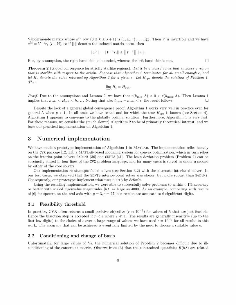
Vandermonde matrix whose kth row (0 ≤ k ≤ s+ 1) is (1, zk, z2k, . . . , z

sk). Then V is invertible and we have

a[i] = V −1ri (i ∈ N), so if |||·||| denotes the induced matrix norm, then

‖a[i]‖ = ‖V −1ri‖ ≤∣∣∣∣∣∣V −1

∣∣∣∣∣∣ ‖ri‖.But, by assumption, the right hand side is bounded, whereas the left hand side is not.

Theorem 2 (Global convergence for strictly starlike regions). Let Λ be a closed curve that encloses a regionthat is starlike with respect to the origin. Suppose that Algorithm 2 terminates for all small enough ε, andlet Hε denote the value returned by Algorithm 2 for a given ε. Let Hopt denote the solution of Problem 1.Then

limε→0

Hε = Hopt.

Proof. Due to the assumptions and Lemma 2, we have that r(hmin,Λ) < 0 < r(hmax,Λ). Then Lemma 1implies that hmin < Hopt < hmax. Noting that also hmax − hmin < ε, the result follows.

Despite the lack of a general global convergence proof, Algorithm 1 works very well in practice even forgeneral Λ when p > 1. In all cases we have tested and for which the true Hopt is known (see Section 4),Algorithm 1 appears to converge to the globally optimal solution. Furthermore, Algorithm 1 is very fast.For these reasons, we consider the (much slower) Algorithm 2 to be of primarily theoretical interest, and webase our practical implementation on Algorithm 1.

3 Numerical implementation

We have made a prototype implementation of Algorithm 1 in Matlab. The implementation relies heavilyon the CVX package [12, 11], a Matlab-based modeling system for convex optimization, which in turn relieson the interior-point solvers SeDuMi [36] and SDPT3 [41]. The least deviation problem (Problem 2) can besuccinctly stated in four lines of the CVX problem language, and for many cases is solved in under a secondby either of the core solvers.

Our implementation re-attempts failed solves (see Section 3.2) with the alternate interfaced solver. Inour test cases, we observed that the SDPT3 interior-point solver was slower, but more robust than SeDuMi.Consequently, our prototype implementation uses SDPT3 by default.

Using the resulting implementation, we were able to successfully solve problems to within 0.1% accuracyor better with scaled eigenvalue magnitudes |hλ| as large as 4000. As an example, comparing with resultsof [6] for spectra on the real axis with p = 3, s = 27, our results are accurate to 6 significant digits.

3.1 Feasibility threshold

In practice, CVX often returns a small positive objective (r ≈ 10−7) for values of h that are just feasible.Hence the bisection step is accepted if r < ε where ε � 1. The results are generally insensitive (up to thefirst few digits) to the choice of ε over a large range of values; we have used ε = 10−7 for all results in thiswork. The accuracy that can be achieved is eventually limited by the need to choose a suitable value ε.

3.2 Conditioning and change of basis

Unfortunately, for large values of hλ, the numerical solution of Problem 2 becomes difficult due to ill-conditioning of the constraint matrix. Observe from (3) that the constrained quantities R(hλ) are related

9

to the decision variables aj through multiplication by a Vandermonde matrix. Vandermonde matrices areknown to be ill-conditioned for most choices of abscissas. For very large hλ, the resulting CVX problem cannotbe reliably solved by either of the core solvers.

A first approach to reducing the condition number of the constraint matrix is to rescale the monomialbasis. We have found that a more robust approach for many types of spectra can be obtained by choosinga basis that is approximately orthogonal over the given spectrum {Λ}. Thus we seek a solution of the form

R(z) =

s∑j=0

ajQj(z) where Qj(z) =

j∑k=0

bjkzk. (10)

Here Qj(z) is a degree-j polynomial chosen to give a well-conditioned constraint matrix. The drawback ofnot using the monomial basis is that the dimension of the problem is s + 1 (rather than s + 1 − p) and wemust now impose the order conditions explicitly:

s∑j=0

ajbjk =1

k!for k = 0, 1, . . . , p. (11)

Consequently, using a non-monomial basis increases the number of design variables in the problem andintroduces an equality constraint matrix B ∈ Rp×s that is relatively small (when p � s), but usually verypoorly conditioned. However, it can dramatically improve the conditioning of the inequality constraints.

The choice of the basis Qj(z) is a challenging problem in general. In the special case of a negative realspectrum, an obvious choice is the Chebyshev polynomials (of the first kind) Tj , shifted and scaled to thedomain [hx, 0] where x = minλ∈Λ Re(λ), via an affine map:

Qj(z) = Tj

(1 +

2z

hx

). (12)

The motivation for using this basis is that |Qj(hλ)| ≤ 1 for all λ ∈ [hx, 0]. This basis is also suggested by thefact that Qj(z) is the optimal stability polynomial in terms of negative real axis inclusion for p = 1, s = j. InSection 4, we will see that this choice of basis works well for more general spectra when the largest magnitudeeigenvalues lie near the negative real axis.

As an example, we consider a spectrum of 3200 equally spaced values λ in the interval [−1, 0]. Theexact solution is known to be h = 2s2. Figure 2 shows the relative error as well as the inequality constraintmatrix condition number obtained by using the monomial (3) and Chebyshev (12) bases. Typically, thesolver is accurate until the condition number reaches about 1016. This supports the hypothesis that it isthe conditioning of the inequality constraint matrix that leads to failure of the solver. The Chebyshev basiskeeps the condition number small and yields accurate answers even for very large values of h.

3.3 Choice of initial upper bound

The bisection algorithm requires as input an initial hmax such that r(hmax,Λ) > 0. Theoretical values canbe obtained using the classical upper bound of 2s2/x if Λ encloses a negative real interval [x, 0], or using theupper bound given in [33] if Λ encloses an ellipse in the left half-plane. Alternatively, one could start witha guess and successively double it until r(hmax,Λ) > 0 is satisfied. Since evaluation of r(h,Λ) is typicallyquite fast, finding a tight initial hmax is not an essential concern.

10

100 101 102 103 104100

1050

10100

10150

h

Con

ditio

n N

umbe

r

Real Axis

100 101 102 103 10410−8

10−6

10−4

10−2

100

Rel

ativ

e Er

ror

Condition Number (Monomial)Relative Error (Monomial)Condition Number (Chebyshev)Relative Error (Chebyshev)

100 101 102100

105

1010

1015

1020

1025

h

Con

ditio

n N

umbe

r

Imaginary Axis

100 101 10210−8

10−6

10−4

10−2

100

Rel

ativ

e Er

ror

100 101 102100

1010

1020

1030

1040

h

Con

ditio

n N

umbe

r

Disc

100 101 10210−8

10−6

10−4

10−2

100

Rel

ativ

e Er

ror

Figure 2: Condition number of principal constraint matrix and relative solution accuracy versus optimalstep size. The points along a given curve correspond to different choices of s.

4 Examples

We now demonstrate the effectiveness of our algorithm by applying it to determine optimally stable poly-nomials (i.e., solve Problem 1) for various types of spectra. As stated above, we use Algorithm 1 for itssimplicity, speed, and effectiveness. When Λ corresponds to an infinite set, we approximate it by a finediscretization.

4.1 Verification

In this section, we apply our algorithm to some well-studied cases with known exact or approximate resultsin order to verify its accuracy and correctness. In addition to the real axis, imaginary axis, and disk casesbelow, we have successfully recovered the results of [28]. Our algorithm succeeds in finding the globallyoptimal solution in every case for which it is known, except in some cases of extremely large step sizes forwhich the underlying solvers (SDPT3 and SeDuMi) eventually fail.

4.1.1 Negative real axis inclusion

Here we consider the largest h such that [−h, 0] ∈ S by taking Λ = [−1, 0]. This is the most heavily studiedcase in the literature, as it applies to the semi-discretization of parabolic PDEs and a large increase of Hopt

is possible when s is increased (see, e.g., [32, 43, 27, 6, 34]). For first-order accurate methods (p = 1), theoptimal polynomials are just shifted Chebyshev polynomials, and the optimal timestep is Hopt = 2s2. Manyspecial analytical and numerical techniques have been developed for this case; the most powerful seems tobe that of Bogatyrev [6].

We apply our algorithm to a discretization of Λ (using 6400 evenly-spaced points) and using the shiftedand scaled Chebyshev basis (12). Results for up to s = 40 are shown in Table 1 (note that we list Hopt/s

2 foreasy comparison, since Hopt is approximately proportional to s2 in this case). We include results for p = 10to demonstrate the algorithm’s ability to handle high-order methods. For p = 1 and 2, the values computedhere match those available in the literature [42]. Most of the values for p = 3, 4 and 10 are new results.Figure 3 shows some examples of stability regions for optimal methods. As observed in the literature, itseems that Hopt/s

2 tends to a constant (that depends only on p) as s increases. For large values of s, some

11

Hopt/s2

Stages p = 1 p = 2 p = 3 p = 4 p = 101 2.0002 2.000 0.5003 2.000 0.696 0.2794 2.000 0.753 0.377 0.1745 2.000 0.778 0.421 0.2426 2.000 0.792 0.446 0.2777 2.000 0.800 0.460 0.2988 2.000 0.805 0.470 0.3119 2.000 0.809 0.476 0.32110 2.000 0.811 0.481 0.327 0.05115 2.000 0.817 0.492 0.343 0.08920 2.000 0.819 0.496 0.349 0.12025 2.000 0.820 0.498 0.352 0.12530 2.001 0.821 0.499 0.353 0.12935 2.000 0.821 0.499 0.354 0.13240 2.000 0.821 0.500 0.355 0.132

Table 1: Scaled size of real axis interval inclusion for optimized methods.

results in the table have an error of about 10−3 due to inaccuracies in the numerical results provided by theinterior point solvers.

4.1.2 Imaginary axis inclusion

Next we consider the largest h such that [−ih, ih] ∈ S by taking Λ = xi, x ∈ [−1, 1]. Optimal polynomials forimaginary axis inclusion have also been studied by many authors, and a number of exact results are knownor conjectured [42, 45, 20, 21, 22, 43]. We again approximate the problem, taking N = 3200 evenly-spacedvalues in the interval [0, i] (note that stability regions are necessarily symmetric about the real axis sinceR(z) has real coefficients). We use a “rotated” Chebyshev basis defined by

Qj(z) = ijTj

(iz

hx

),

where x = maxi(| Im(λi)|). Like the Chebyshev basis for the negative real axis, this basis dramaticallyimproves the robustness of the algorithm for imaginary spectra. Table 2 shows the optimal effective stepsizes. In agreement with [42, 21], we find H = s − 1 for p = 1 (all s) and for p = 2 (s odd). We alsofind H = s − 1 for p = 1 and s even, which was conjectured in [45] and confirmed in [43]. We findHopt =

√s(s− 2) for p = 2 and s even, strongly suggesting that the polynomials given in [20] are optimal

for these cases; on the other hand, our results show that those polynomials, while third order accurate, arenot optimal for p = 3 and s odd. Figure 4 shows some examples of stability regions for optimal methods.

4.1.3 Disk inclusion

In the literature, attention has been paid to stability regions that include the disk

D(h) = {z : |1 + z/h| ≤ 1}, (13)

12

140 120 100 80 60 40 20 010

0

10

(a) p = 4, s = 20

140 120 100 80 60 40 20 010

0

10

(b) p = 10, s = 20

Figure 3: Stability regions of some optimal methods for real axis inclusion.

Hopt/sStages p = 1 p = 2 p = 3 p = 42 0.5003 0.667 0.667 0.5774 0.750 0.708 0.708 0.7075 0.800 0.800 0.783 0.6936 0.833 0.817 0.815 0.8167 0.857 0.857 0.849 0.8138 0.875 0.866 0.866 0.8669 0.889 0.889 0.884 0.86410 0.900 0.895 0.895 0.89415 0.933 0.933 0.932 0.92520 0.950 0.949 0.949 0.94925 0.960 0.960 0.959 0.95730 0.967 0.966 0.966 0.96635 0.971 0.971 0.971 0.97040 0.975 0.975 0.975 0.97545 0.978 0.978 0.978 0.97750 0.980 0.980 0.980 0.980

Table 2: Scaled size of imaginary axis inclusion for optimized methods.

13

6 4 2 0

6

4

2

0

2

4

6

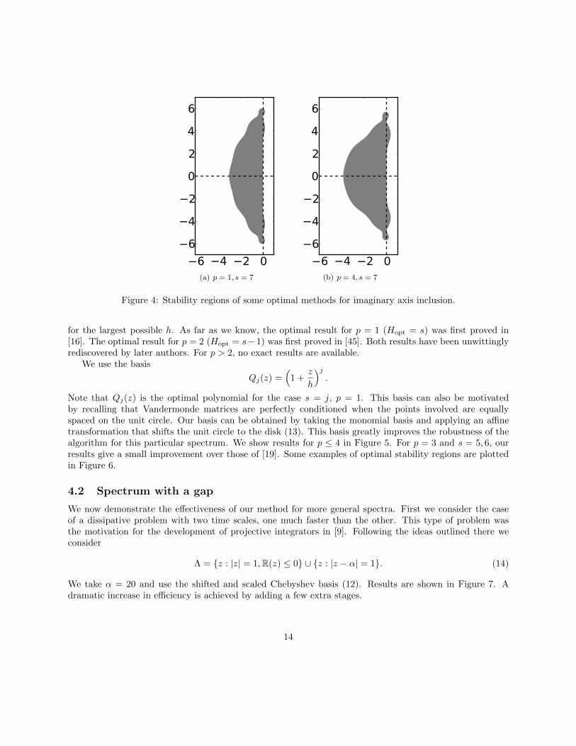
(a) p = 1, s = 7

6 4 2 0

6

4

2

0

2

4

6

(b) p = 4, s = 7

Figure 4: Stability regions of some optimal methods for imaginary axis inclusion.

for the largest possible h. As far as we know, the optimal result for p = 1 (Hopt = s) was first proved in[16]. The optimal result for p = 2 (Hopt = s−1) was first proved in [45]. Both results have been unwittinglyrediscovered by later authors. For p > 2, no exact results are available.

We use the basis

Qj(z) =(

1 +z

h

)j.

Note that Qj(z) is the optimal polynomial for the case s = j, p = 1. This basis can also be motivatedby recalling that Vandermonde matrices are perfectly conditioned when the points involved are equallyspaced on the unit circle. Our basis can be obtained by taking the monomial basis and applying an affinetransformation that shifts the unit circle to the disk (13). This basis greatly improves the robustness of thealgorithm for this particular spectrum. We show results for p ≤ 4 in Figure 5. For p = 3 and s = 5, 6, ourresults give a small improvement over those of [19]. Some examples of optimal stability regions are plottedin Figure 6.

4.2 Spectrum with a gap

We now demonstrate the effectiveness of our method for more general spectra. First we consider the caseof a dissipative problem with two time scales, one much faster than the other. This type of problem wasthe motivation for the development of projective integrators in [9]. Following the ideas outlined there weconsider

Λ = {z : |z| = 1,R(z) ≤ 0} ∪ {z : |z − α| = 1}. (14)

We take α = 20 and use the shifted and scaled Chebyshev basis (12). Results are shown in Figure 7. Adramatic increase in efficiency is achieved by adding a few extra stages.

14

0 10 20 30 40 50 60 70 80s

0.4

0.5

0.6

0.7

0.8

0.9

1.0

1.1

Hopt/s

p=1p=2p=3p=4

Figure 5: Relative size of largest disk that can be included in the stability region (scaled by the number ofstages).

25 20 15 10 5 015

10

5

0

5

10

15

(a) p = 3, s = 8

25 20 15 10 5 015

10

5

0

5

10

15

(b) p = 4, s = 15

Figure 6: Stability regions of some optimal methods for disk inclusion.

15

(a) Optimal effective step size

40 30 20 10 010

5

0

5

10

(b) Optimal stability region for p = 1, s = 6, α = 20 (stable step size≈ 1.975)

Figure 7: Optimal methods for spectrum with a gap (14) with α = 20.

4.3 Legendre pseudospectral discretization

Next we consider a system obtained from semidiscretization of the advection equation on the interval [−1, 1]with homogeneous Dirichlet boundary condition:

ut = ux u(t, x = 1) = 0.

The semi-discretization is based on pseudospectral collocation at points given by the zeros of the Legendrepolynomials; we take N = 50 points. The semi-discrete system takes the form (1), where L is the Legendredifferentiation matrix, whose eigenvalues are shown in Figure 8(a). We compute an optimally stable poly-nomial based on the spectrum of the matrix, taking s = 7 and p = 1. The stability region of the resultingmethod is plotted in Figure 8(c). Using an appropriate step size, all the scaled eigenvalues of L lie in thestability region. However, this method is unstable in practice for any positive step size; Figure 8(e) showsan example of a computed solution after three steps, where the initial condition is a Gaussian. The resultinginstability is non-modal, meaning that it does not correspond to any of the eigenvectors of L (compare [40,Figure 31.2]).

This discretization is now well-known as an example of non-normality [40, Chapters 30-32]. Due to thenon-normality, it is necessary to consider pseudospectra in order to design an appropriate integration scheme.The ε-pseudospectrum (see [40]) is the set

{z ∈ C : ‖(z −D)−1‖ > 1/ε}.

The ε-pseudospectrum (for ε = 2) is shown with the eigenvalues in Figure 8(b). The instability observedabove occurs because the stability region does not contain an interval on the imaginary axis about the origin,whereas the pseudospectrum includes such an interval.

We now compute an optimally stable integrator based on the 2-pseudospectrum. This pseudospectrumis computed using an approach proposed in [39, Section 20], with sampling on a fine grid. In order to reducethe number of constraints and speed up the solution, we compute the convex hull of the resulting set andapply our algorithm. The resulting stability region is shown in Figure 8(d). It is remarkably well adapted;notice the two isolated roots that ensure stability of the modes corresponding to the extremal imaginaryeigenvalues. We have verified that this method produces a stable solution, in agreement with theory (see

16

Chapter 32 of [40]); Figure 8(f) shows an example of a solution computed with this method. The initialGaussian pulse advects to the left.

4.4 Thin rectangles

A major application of explicit Runge–Kutta methods with many stages is the solution of moderately stiffadvection-reaction-diffusion problems [15, 44]. For such problems, the stability region must include not onlya large interval on the negative real axis, but also some region around it, due to convective terms. If centereddifferences are used for the advective terms, it is natural to require that a small interval on the imaginaryaxis be included. Hence, one may be interested in methods that contain a rectangular region

Λκ = {λ ∈ C : −β ≤ Im(λ) ≤ β, −κ ≤ Re(λ) ≤ 0}. (15)

for given κ, β. No methods optimized for such regions appear in the literature, and the available approachesfor devising methods with extended real axis stability (including those of [37]) cannot be applied to suchregions. Because of this, previously existing methods are applicable only if upwind differencing is applied toconvective terms [44, 37].

For this example, rather than parameterizing by the step size h, we assume that a desired step size hand imaginary axis limit β are given based on the convective terms, which generally require small step sizesfor accurate resolution. We seek to find (for given s, p) the polynomial (3) that includes Λκ for κ as largeas possible. This could correspond to selection of an optimal integrator based on the ratio of convective anddiffusive scales (roughly speaking, the Reynolds number). Since the desired stability region lies relativelynear the negative real axis, we use the shifted and scaled Chebyshev basis (12).

Stability regions of some optimal methods are shown in Figure 9. The outline of the included rectangleis superimposed in black. The stability region for β = 10, s = 20, shown in Figure 9 is especially interestingas it is very nearly rectangular. A closeup view of the upper boundary is shown in Figure 10.

5 Discussion

The approach described here can speed up the integration of IVPs for which

• explicit Runge–Kutta methods are appropriate;

• the spectrum of the problem is known or can be approximated; and

• stability is the limiting factor in choosing the step size.

Although we have considered only linear initial value problems, we expect our approach to be useful indesigning integrators for nonlinear problems via the usual approach of considering the spectrum of theJacobian. A first successful application of our approach to nonlinear PDEs appears in [29].

The amount of speedup depends strongly on the spectrum of the problem, and can range from a fewpercent to several times or more. Based on past work and on results presented in Section 4, we expectthat the most substantial gains in efficiency will be realized for systems whose spectra have large negativereal parts, such as for semi-discretization of PDEs with significant diffusive or moderately stiff reactioncomponents. As demonstrated in Section 4, worthwhile improvements may also be attained for generalsystems, and especially for systems whose spectrum contains gaps.

The work presented here suggests several extensions and areas for further study. For very high polynomialdegree, the convex subproblems required by our algorithm exhibit poor numerical conditioning. We have

17

−200 −100 0−150

−100

−50

0

50

100

150

(a) Eigenvalues.

−200 −100 0−150

−100

−50

0

50

100

150

(b) Eigenvalues and pseudospec-trum (the boundary of the 2-pseudospectrum is plotted).

8 6 4 2 08

6

4

2

0

2

4

6

8

(c) Optimized stability regionbased on eigenvalues.

8 6 4 2 08

6

4

2

0

2

4

6

8

(d) Optimized stability regionbased on pseudospectrum.

−1 −0.5 0 0.5 1−2

−1

0

1

2

3x 1012

(e) Solution computed withmethod based on spectrum.

−1 −0.5 0 0.5 10

0.2

0.4

0.6

0.8

1

(f) Solution computed with methodbased on pseudospectrum.

Figure 8: Results for the Legendre differentiation matrix with N = 50.

18

80 70 60 50 40 30 20 10 020

15

10

5

0

5

10

15

20

(a) β = 1, p = 1, s = 10

80 70 60 50 40 30 20 10 020

15

10

5

0

5

10

15

20

(b) β = 10, p = 1, s = 20

Figure 9: Stability regions of some optimal methods for thin rectangle inclusion.

Figure 10: Closeup view of upper boundary of the rectangular stability region plotted in Figure 9.

proposed a first improvement by change of basis, but further improvements in this regard could increase therobustness and accuracy of the algorithm. It seems likely that our algorithm exhibits global convergence ingeneral circumstances beyond those for which we have proven convergence. The question of why bisectionseems to always lead to globally optimal solutions merits further investigation. While we have focusedprimarily on design of the stability properties of a scheme, the same approach can be used to optimizeaccuracy efficiency, which is a focus of future work. Our algorithm can also be applied in other ways; forinstance, it could be used to impose a specific desired amount of dissipation for use in multigrid or as a kindof filtering.

We remark that the problem of determining optimal polynomials subject to convex constraints is verygeneral. Convex optimization techniques have already been exploited to solve similar problems in filterdesign [8], and will likely find further applications in numerical analysis.

Acknowledgments. We thank Lajos Loczi for providing a simplification of the proof of Lemma 3. Weare grateful to R.J. LeVeque and L.N. Trefethen for helpful comments on a draft of this work.

References

[1] A. Abdulle, On roots and error constants of optimal stability polynomials, BIT Numerical Mathemat-ics, 40 (2000), pp. 177–182.

[2] , Fourth order Chebyshev methods with recurrence relation, SIAM Journal on Scientific Computing,23 (2002), pp. 2041–2054.

19

[3] A. Abdulle and A. Medovikov, Second order Chebyshev methods based on orthogonal polynomials,Numerische Mathematik, 90 (2001), pp. 1–18.

[4] V. Allampalli, R. Hixon, M. Nallasamy, and S. D. Sawyer, High-accuracy large-step explicitRunge-Kutta (HALE-RK) schemes for computational aeroacoustics, Journal of Computational Physics,228 (2009), pp. 3837–3850.

[5] M. Bernardini and S. Pirozzoli, A general strategy for the optimization of Runge-Kutta schemesfor wave propagation phenomena, Journal of Computational Physics, 228 (2009), pp. 4182–4199.

[6] A. B. Bogatyrev, Effective solution of the problem of the optimal stability polynomial, Sbornik: Math-ematics, 196 (2005), pp. 959–981.

[7] J. Butcher, Numerical Methods for Ordinary Differential Equations, Wiley, second ed., 2008.

[8] T. Davidson, Enriching the Art of FIR Filter Design via Convex Optimization, IEEE Signal ProcessingMagazine, 27 (2010), pp. 89–101.

[9] C. W. Gear and I. G. Kevrekidis, Projective Methods for Stiff Differential Equations: Problemswith Gaps in Their Eigenvalue Spectrum, SIAM Journal on Scientific Computing, 24 (2003), p. 1091.

[10] S. Gottlieb, D. I. Ketcheson, and C.-W. Shu, Strong stability preserving Runge–Kutta and mul-tistep time discretizations, World Scientific Publishing Company, 2011.

[11] M. Grant and S. Boyd, Graph implementations for nonsmooth convex programs, in Recent Advancesin Learning and Control, V. Blondel, S. Boyd, and H. Kimura, eds., Lecture Notes in Control andInformation Sciences, Springer-Verlag Limited, 2008, pp. 95–110.

[12] , CVX: MATLAB software for disciplined convex programming. http://cvxr.com/cvx, Apr. 2011.

[13] E. Hairer, , and G. Wanner, Solving ordinary differential equations II: Stiff and differential-algebraicproblems, Springer, second ed., 1996.

[14] R. Hettich, Semi-Infinite Programming: Theory, Methods, and Applications, SIAM review, 35 (1993),pp. 380–429.

[15] W. Hundsdorfer and J. G. Verwer, Numerical solution of time-dependent advection-diffusion-reaction equations, vol. 33, Springer, 2003.

[16] R. Jeltsch and O. Nevanlinna, Largest disk of stability of explicit Runge–Kutta methods, BITNumerical Mathematics, 18 (1978), pp. 500–502.

[17] , Stability of explicit time discretizations for solving initial value problems, Numerische Mathe-matik, 37 (1981), pp. 61–91.

[18] , Stability and accuracy of time discretizations for initial value problems, Numerische Mathematik,40 (1982), pp. 245–296.

[19] R. Jeltsch and M. Torrilhon, Flexible stability domains for explicit Runge–Kutta methods, Sometopics in industrial and applied mathematics, (2007), p. 152.

[20] I. P. Kinnmark and W. G. Gray, One step integration methods of third-fourth order accuracy withlarge hyperbolic stability limits, Mathematics and Computers in Simulation, 26 (1984), pp. 181–188.

20

[21] , One step integration methods with maximum stability regions, Mathematics and Computers inSimulation, 26 (1984), pp. 87–92.

[22] I. P. E. Kinnmark and W. G. Gray, Fourth-order accurate one-step integration methods with largeimaginary stability limits, Numerical Methods for Partial Differential Equations, 2 (1986), pp. 63–70.

[23] J. Lawson, An order five Runge–Kutta process with extended region of stability, SIAM Journal onNumerical Analysis, (1966).

[24] R. J. LeVeque, Finite Difference Methods for Ordinary and Partial Differential Equations, SIAM,Philadelphia, 2007.

[25] J. Martin-Vaquero and B. Janssen, Second-order stabilized explicit Runge–Kutta methods for stiffproblems, Computer Physics Communications, 180 (2009), pp. 1802–1810.

[26] J. L. Mead and R. A. Renaut, Optimal Runge–Kutta methods for first order pseudospectral operators,Journal of Computational Physics, 152 (1999), pp. 404–419.

[27] A. A. Medovikov, High order explicit methods for parabolic equations, BIT Numerical Mathematics,38 (1998), pp. 372–390.

[28] J. Niegemann, R. Diehl, and K. Busch, Efficient low-storage Runge-Kutta schemes with optimizedstability regions, Journal of Computational Physics, 231 (2011), pp. 372–364.

[29] M. Parsani et al., Optimal explicit Runge–Kutta schemes for the spectral difference method appliedto Euler and linearized Euler equations. In Preparation.

[30] J. Pike and P. Roe, Accelerated convergence of Jameson’s finite-volume Euler scheme using van derHouwen integrators, Computers & Fluids, 13 (1985), pp. 223–236.

[31] R. Renaut, Two-step Runge-Kutta methods and hyperbolic partial differential equations, Mathematicsof Computation, 55 (1990), pp. 563–579.

[32] W. Riha, Optimal stability polynomials, Computing, 9 (1972), pp. 37–43.

[33] J. M. Sanz-Serna and M. N. Spijker, Regions of stability, equivalence theorems and the Courant-Friedrichs-Lewy condition, Numerische Mathematik, 49 (1986), pp. 319–329.

[34] L. M. Skvortsov, Explicit stabilized Runge–Kutta methods, Computational Mathematics and Mathe-matical Physics, 51 (2011), pp. 1153–1166.

[35] B. Sommeijer and J. G. Verwer, On stabilized integration for time-dependent PDEs, Journal ofComputational Physics, 224 (2007), pp. 3–16.

[36] J. Sturm, Using sedumi 1.02, a matlab toolbox for optimization over symmetric cones, Optimizationmethods and software, 11 (1999), pp. 625–653.

[37] M. Torrilhon and R. Jeltsch, Essentially optimal explicit Runge-Kutta methods with applicationto hyperbolicparabolic equations, Numerische Mathematik, 106 (2007), pp. 303–334.

[38] T. Toulorge and W. Desmet, Optimal Runge–Kutta Schemes for Discontinuous Galerkin SpaceDiscretizations Applied to Wave Propagation Problems, Journal of Computational Physics, (2011).

21

[39] L. Trefethen, Computation of pseudospectra, Acta numerica, 8 (1999), pp. 247–295.

[40] L. Trefethen and M. Embree, Spectra and Pseudospectra: The Behavior of Nonnormal Matricesand Operators, Princeton University Press, Princeton, 2005.

[41] R. Tutuncu, K. Toh, and M. Todd, Solving semidefinite-quadratic-linear programs using sdpt3,Mathematical programming, 95 (2003), pp. 189–217.

[42] P. van der Houwen, Explicit Runge–Kutta Formulas with Increased Stability Boundaries, NumerischeMathematik, 20 (1972), pp. 149–164.

[43] P. J. van der Houwen, The development of Runge–Kutta methods for partial differential equations,Applied Numerical Mathematics, 20 (1996), pp. 261–272.

[44] J. G. Verwer, B. Sommeijer, and W. Hundsdorfer, RKC time-stepping for advection-diffusion-reaction problems, Journal of Computational Physics, 201 (2004), pp. 61–79.

[45] R. Vichnevetsky, New stability theorems concerning one-step numerical methods for ordinary differ-ential equations, Mathematics and Computers in Simulation, 25 (1983), pp. 199–205.

22