Applications of Numerical Optimal Control to

Nonlinear Hybrid Systems

Shangming Wei a, Kasemsak Uthaichana b, Milos Zefran a,Raymond A. DeCarlo b,∗, Sorin Bengea c

aDepartment of Electrical and Computer Engineering, University of Illinois atChicago, Chicago, Illinois, USA

bSchool of Electrical and Computer Engineering, Purdue University, WestLafayette, Indiana, USA

cInnovation Center, Decision and Control Group, Eaton Corporation, EdenPrairie, Minnesota

Abstract

This paper develops a technique for numerically solving hybrid optimal control prob-lems. The theoretical foundation of the approach is a recently developed methodol-ogy by Bengea & DeCarlo [1] for solving switched optimal control problems throughembedding. The methodology is extended to incorporate hybrid behavior stemmingfrom autonomous (uncontrolled) switches that results in the plant equations withpiecewise smooth vector fields. We demonstrate that when the system has no mem-ory, the embedding technique can be used to reduce the hybrid optimal controlproblem for such systems to the traditional one. In particular, we show that thesolution methodology does not require mixed integer programming (MIP) meth-ods, but rather can utilize traditional nonlinear programming techniques such assequential quadratic programming (SQP). By dramatically reducing the computa-tional complexity over existing approaches, the proposed techniques make optimalcontrol highly appealing for hybrid systems. This appeal is concretely demonstratedin an exhaustive application to a unicycle model that contains both autonomousand controlled switches; optimal and model predictive control solutions are givenfor two types of models using both a minimum energy and minimum time perfor-mance index. Controller performance is evaluated in the presence of a step frictionaldisturbance which demonstrates the robustness of the controllers.

Key words: Hybrid systems, optimal control, numerical optimization, modelpredictive control

∗ Corresponding author.Email addresses: swei3@uic.edu (Shangming Wei), uthaicha@purdue.edu

Preprint submitted to Nonlinear Analysis TMA 28 June 2006

1 Introduction

Hybrid systems have arisen as a powerful paradigm for describing systems thatare characterized by a combination of continuous-valued and discrete-valuedvariables. A wealth of literature is available for the modeling and control ofhybrid systems and we refer the reader to the overview articles [2, 3] and thebooks [4, 5]. A number of authors have also considered optimal control of hy-brid systems. In general, the problem is quite hard as it involves both elementsof optimal control as well as combinatorial optimization. The hybrid optimalcontrol problems of [6], [7], [8], and [9] have led to generalizations of the Max-imum Principle. For certain optimization problems, there exist numericallysound algorithms for obtaining suboptimal solutions. For example, one canuse a hybrid version of the Bellman inequality, as in [10], or mixed integerprogramming (MIP), as in [11]. Industrial experience and simulations showthat the performance of the solutions obtained by means of these methodsare satisfactory, although these methods in general do not scale well. An al-gorithm based on a dynamic programming approach is proposed in [12, 13].For a pre-assigned switching sequence (fixed number of switches and fixedmode sequence), a method for solving an optimization problem was describedin [14], and for linear autonomous systems subject to a quadratic cost in [15].A general setup uses viscosity solution techniques: the value functions asso-ciated with each mode of operation are shown to be solutions of a system ofquasivariational inequalities in a weak sense; the optimal controls are thencomputed using PDE methods. Such an approach is used in [16] for solving anoptimization problem associated with a switched system with time-invariantautonomous subsystems. A general optimal hybrid control problem which en-ables a direct Maximum Principle approach was presented in [17]. However,this work discusses neither sufficient conditions for optimality nor the singularcases.

The primary focus of this paper is the development of optimal and modelpredictive control (MPC) [18] solutions to the hybrid optimal control problemwhen the plant admits both autonomous and controlled switches. As such weinvestigate the numerical solution of the problem assuming the autonomousswitches are memoryless. Specifically we develop an extension of embeddingtechnique of Bengea and DeCarlo [1] for the solution of the hybrid optimal(switched) control problem to the case of piecewise smooth vector fields inthe plant equations which result in the presence of memoryless autonomousswitches.

(Kasemsak Uthaichana), mzefran@uic.edu (Milos Zefran),decarlo@ecn.purdue.edu (Raymond A. DeCarlo), sbengea@ieee.org (SorinBengea).

2

It is generally perceived that the best numerical methods available for hybridoptimal control problems involve mixed integer programming (MIP). Whilegreat progress has been made in recent years in improving these methods,the MIP is an NP-hard problem so scalability is problematic. However, in ourcontext, the solution methodology does not require a mixed integer program-ming problem (MIP) but rather can utilize traditional nonlinear programmingtechniques such as sequential quadratic programming (SQP). By dramaticallyreducing the computational complexity over existing approaches, the proposedtechniques make optimal control highly appealing for hybrid systems. Thisappeal is concretely demonstrated in an exhaustive application to a unicyclemodel that contains both autonomous and controlled switches; optimal andmodel predictive control solutions are given for two types of models. Twoperformance indexes are set forth: a minimum energy and minimum time.Controller performance is evaluated in the presence of a step frictional distur-bance which demonstrates the robustness of the controllers.

The paper is organized as follows. We start by presenting our modeling frame-work and introducing the terminology used in the paper. Section 3 formulatesthe optimal control problem for systems that undergo both autonomous andcontrolled switches. We show how to extend the method from [1] so that hybridoptimal control problem can be embedded as a traditional smooth problem.We then turn to a set of examples to demonstrate how to develop numeri-cal methods for the resulting smooth problem. We conclude the paper with ashort discussion and the possibilities for future work.

2 Mathematical Preliminaries

The hybrid systems studied in this paper will come from the class of switchedsystems. In particular, we are interested in control systems that exhibit twotypes of switching behavior, both resulting in discontinuous jumps in the vec-tor fields governing the evolution of the continuous state of the system. First,we are interested in systems where the vector fields undergo discontinuousjumps as a result of the state and the input entering different regions in thecombined state and input space. We call such switches autonomous or un-controlled to indicate that the switches can not be effected directly througha separate switching mechanism. An example of a system with autonomousswitches is a system subject to continuous state dependent constraints, wherethe autonomous switches correspond to different combinations of constraintsthat are active in a particular continuous state. The second type of switches in-volves discontinuous jumps in the vector fields that can be directly controlled,thus called the controlled switches. An example of a system with controlledswitches is a continuous control system that can be controlled by a finitenumber of different continuous controllers, where the controller to be used is

3

determined by a supervisory controller. In this paper we assume that the setof different operating regimes of the system defined through the autonomousand controlled switches is finite.

In order to describe the evolution of a control system subject to controlledand autonomous switches we need four quantities: (i) the discrete state ξ(t) ∈Dξ = 1, 2, . . . , dξ, (ii) the continuous state x(t) ∈ Rn, (iii) the discretecontrol input (switching control input) v(t) ∈ Dv = 1, 2, . . . , dv, and (iv)the continuous control input u(t) ∈ Rm. The discrete state of the systemdescribes the autonomous switches. In this paper we only consider systemsfor which the autonomous switches depend on the continuous state x(t) andthe input u(t), they do not depend on the current discrete state ξ(t). Suchsystems are usually called memoryless. Formally, the evolution of the discretestate of the memoryless system is defined by a piecewise continuous 1 functionη : Rn × Rm → Dξ, that for each continuous state x and continuous controlinput u selects the discrete state ξ of the system:

ξ+(t) = η(x, u). (1)

Let Mi ⊆ Rn × Rm, i ∈ Dξ be the set of pairs (x, u) corresponding to thediscrete state i ∈ Dξ:

Mi = (x, u) ∈ Rn × Rm | η(x, u) = i,

and let f(i,j), i ∈ Dξ, j ∈ Dv be a collection of C1 vector fields

f(i,j) : Mi → Rn.

The evolution of the continuous state x(t) is then described by:

x(t) = f(η(x(t),u(t)),v(t))(x(t), u(t)), x(t0) = x0. (2)

At each t ≥ t0 and for each discrete state ξ(t) ∈ Dξ, the switching controlinput v(t) ∈ Dv thus selects which of the dv vector fields governs the evolutionof the continuous state. We will assume that the continuous control input u(t)is constrained to the convex and compact set Ω ⊆ Rm and that the switchingcontrol input v(t) and the continuous control input u(t) are both measurablefunctions. Note that in this paper we restrict our attention to time-invariantsystems, but the results can be easily generalized to time-varying systems.

1 By piecewise continuous we mean a function that is continuous everywhere excepton a finite union of switching surfaces that are smooth submanifolds of Rn × Rm

with measure 0 where it undergoes discontinuous jumps, but has well defined limitsin all directions.

4

Given that the discrete state ξ(t) is completely determined by x(t) and u(t)through Eq. (1), we can define for each j ∈ Dv a piecewise C1 vector field 2 :

fj(x(t), u(t)) , f(η(x(t),u(t)),j)(x(t), u(t)) (3)

and rewrite Eq. (2) simply as:

x(t) = fv(t)(x(t), u(t)), x(t0) = x0. (4)

We note that the switching behavior described by Eq. (2) has a special struc-ture since the switching control input v(t) does not affect the autonomousswitches. This means the vector fields fj all have the same set of pointsof discontinuity. We will thus refer to the systems described by Eq. (2) assystems with decoupled switches.

We are interested in computing optimal control laws for the system describedby Eq. (2) or Eq. (4). If the system only undergoes autonomous switches(Dv = 1) only the continuous input u(t) needs to be computed. This sug-gests that the complexity of the optimal control problem might not be anydifferent than in the traditional case. In contrast, for systems with controlledswitches we need to compute the sequence of switching times t1, . . . , tn (in-cluding n), the sequence of discrete inputs ν1, . . . , νn, as well as the continuousinput u(t) on each interval [ti, ti+1) for i = 0, . . . , n. It would therefore appearthat for systems with controlled switches the optimal control problem has com-binatorial complexity. In this paper we show that actually both these caseshave the same complexity and are amenable to traditional nonlinearprogramming techniques such as sequential quadratic programming(SQP). This further implies that for the systems considered in this paperthe optimal control problem is no more complex than the traditional smoothproblem.

In general, the behavior of switched systems can be quite complex and mightlead to anomalies such as Zeno behavior or deadlock states. Furthermore, thesystems in Eq. (2) or Eq. (4) belong to the class of systems with discontinuousright-hand sides [19] so the questions of existence and uniqueness of solutionshave to be carefully studied. While certainly important, these issues are outsidethe scope of this paper and we will assume that the existence and uniqueness(in the appropriate sense) are guaranteed. We refer the interested reader toconference series [20,21], special issues [22–24], and [25,26] for further reading.

2 Similarly as before, by piecewise C1 we mean a function that is C1 everywhereexcept on a finite union of switching surfaces that are smooth submanifolds ofRn × Rm with measure 0 where the function is not differentiable and undergoesdiscontinuous jumps, but has well defined limits in all directions.

5

3 Optimal Control Problem

We now formulate the optimal control problem for hybrid systems describedby Eq. (4). Given that the switching control input is completely arbitrary andindependent from the continuous control, the search for the optimal solutioncan be seen as having three stages [9]: (i) finding the optimal sequence ofcontrol modes (the sequence of values of v); (ii) finding the optimal switchinginstants; and (iii) finding the optimal value for the continuous control. Effec-tively, (i) and (ii) constitute the search for v(t), while (iii) is the search foru(t) given v(t). This partition of the hybrid optimal control problem is the ap-proach pursued in [13–15]. Clearly, (i) results in the combinatorial complexityof the optimal control problem which makes finding the solution challenging atbest. In [11] and the first author’s subsequent work, it was shown that mixedinteger programming (MIP) can be employed to find the optimal solution.However, despite the availability of sophisticated methods for MIP, the com-putational complexity of hybrid optimal control problems still severely limitsthe application of these techniques in practice.

In this section we show that for quite a general class of hybrid optimal controlproblems, the computational complexity of the problem is no greater than thatof smooth optimal control problems. In other words, the combinatorial aspectof the problem can be effectively eliminated, leading to a dramatic reductionin the overall computational cost. Our approach is based on the breakthroughresult in [1], where it was shown that for a system with two discrete modes,the switched optimal control problem can be embedded into a larger familyof systems where the switching function takes values in the interval [0, 1] asopposed to the discrete set 0, 1. The optimal solution of the embeddedsystem is either the solution of the original problem, or can be approximatedarbitrarily closely with a trajectory of the switched system. This essentiallytransforms the switched optimal control problem into a smooth problem thatcan be solved using traditional numerical methods. We show that the approachfrom [1] can be readily extended to systems with an arbitrary number of modeswithout further increase in complexity. Finally, we demonstrate the methodon a nonlinear hybrid system with decoupled switches.

3.1 Problem Formulation

Consider the system described by Eq. (4). Both v(t) and u(t) are controlvariables and for the optimal control problem we require that they are chosenon the interval [t0, tf ] so that the following initial and terminal constraints aresatisfied: (t0, x(t0)) ∈ T0 × B0 and (tf , x(tf )) ∈ Tf × Bf . We will assume thatthe endpoint constraint set B = T0 × B0 × Tf × Bf is contained in a compact

6

set in R2n+2. We define the optimization functional

JC(t0, x0, u, v) = g(t0, x0, tf , xf ) +∫ tf

t0f 0

(η(x(t),u(t)),v(t))(x(t), u(t))dt, (5)

where g is a real-valued C1 function defined on a neighborhood of B, andthe functions f 0

(i,j) : Mi → R, i ∈ Dξ, j ∈ Dv are of class C1. Given thatthe evolution of the discrete state ξ(t) is governed by Eq. (1), we can definesimilarly as in Eq. (3) for each j ∈ Dv a new piecewise C1 function

f 0j (x(t), u(t)) , f 0

(η(x(t),u(t)),j)(x(t), u(t)), (6)

and rewrite the cost functional as:

JC(t0, x0, u, v) = g(t0, x0, tf , xf ) +∫ tf

t0f 0

v(t)(x(t), u(t))dt. (7)

We now define the hybrid optimal control problem for systems with decoupledswitches (HOCD):

minv,u

JC(t0, x0, u, v)

subject to the constraints: (i) x(·) satisfies Eq. (4); (ii) (t0, x(t0), tf , x(tf )) ∈ B;(iii) for each t ∈ [t0, tf ], v(t) ∈ Dv and u(t) ∈ Ω. Except for the fact that thevector fields in question are only piecewise C1, this formulation is similar tothat in [12, 17, 27] where the Maximum Principle is applied directly to theformulation. The formulation can be seen as a special case of the very generalformulations of [9] and [6]. If the switching sequence were fixed, then theproblem formulation would be similar to the one in [14], and if in addition thesystems were linear and the cost functional quadratic, to that in [15].

3.2 Embedding

We now embed system (4) into a larger set of systems. For HOCD, v(t) ∈ D =1, 2, . . . , dv. Introduce dv new variables vi ∈ [0, 1], i ∈ Dv, that satisfy

dv∑i=1

vi(t) = 1. (8)

Let ui be the control input for each vector field fi, i ∈ Dv, in (2). Now definea new system:

x(t) =dv∑i=1

vi(t)fi(x(t), ui(t)), x(t0) = x0, (9)

7

and the associated cost functional

JE(t0, x0, u, v) = g(t0, x0, tf , xf ) +∫ tf

t0

dv∑i=1

vi(t)f0i (x(t), ui(t))dt. (10)

Equations (9) and (10) are the generalization of those in [1]. The HOCDnow becomes the embedded optimal control problem (EOC): minimize thefunctional (10) over all functions vi and ui subject to the following con-straints: (i) x(·) satisfies Eq. (9); (ii) (t0, x(t0), tf , x(tf )) ∈ B; (iii) for eacht ∈ [t0, tf ] and each i ∈ Dv, vi(t) ∈ [0, 1] and ui(t) ∈ Ω; and (iv) for eacht ∈ [t0, tf ],

∑dvi=1 vi(t) = 1.

As in [1] we note that EOC is now amenable to the classical necessary andsufficient conditions of optimal control theory [28]. Furthermore, it can beeasily seen that the set of trajectories of the embedded system (9) containsthe trajectories of the hybrid system (2). But what is crucial for solving theHOCD problem is the following observation.

Proposition 1. The set of trajectories of the hybrid system (2) is dense (inthe L∞ sense) in the set of trajectories of the embedded system (9).

Proof. The proof is analogous to the proof in [1] and proceeds through con-structing a relaxation of the system (9), for which the trajectories of (2) arealso dense. In this process it can be also derived how to explicitly find thetrajectory of (2) that approximates arbitrarily closely a given trajectory of(9).

Because of the fact that the trajectories of (2) are dense in the set of trajec-tories of (9) and since the functions f 0

i in (5) and (10) are C1, we can statethe following proposition.

Proposition 2 (Bengea & DeCarlo [1]). If one of the optimal trajectories,x∗E(·), of the EOC has the property that x∗E(tf ) ∈ Int(Bf )

3 , then either (a)the HOCD has a solution, x∗C(·), which is also a solution of the EOC or (b)the HOCD does not have a solution and suboptimal admissible trajectories ofthe system (2) can be constructed.

The proposition implies that if one first solves the EOC and obtains a solution,either the solution is of the switched type (exactly one of the vi’s is 1 and allthe others are 0), or suboptimal trajectories of the HOCD can be constructedthat can approach the value of the cost for EOC arbitrarily closely and satisfythe boundary conditions within ε for arbitrary ε > 0. Clearly, for practicalapplications this is an extremely valuable observation, given that traditionalnumerical methods can be used to solve EOC.

3 For a set B, Int(B) denotes its interior.

8

Note also that for systems that only exhibit autonomous switches (Dv = 1),no embedding is necessary and except for the fact that the functions f and f 0

are only piecewise C1, the optimal control problem in this case is no differentfrom the traditional formulation. This fact is often overlooked in the literature.

4 Numerical Method

In order to numerically solve the embedded optimal control problem formu-lated in Section 3.2, any numerical method appropriate for traditional optimalcontrol can be used. We refer the reader to [29, 30] for a discussion of suchmethods. In our work, we use a variation of direct collocation [31]. In this case,u(t) and x(t) are chosen from finite-dimensional spaces. Given basis functionsφjN

j=1 and ψjMj=1,

xi =N∑

j=1

pjiφ

j(t), pji ∈ R, i = 1, . . . , n,

ui =M∑

j=1

qjiψ

j(t), qji ∈ R, i = 1, . . . ,m.

Since f is only piecewise C1 and as a result x(t) can be nonsmooth, the basisfunctions φjN

j=1 are chosen to be nonsmooth. Similarly, since the control u(t)can be discontinuous, the basis functions ψjM

j=1 are chosen to be discontin-uous. We start by choosing a discretization of the time interval [t0, tf ]

t0 = t1 < t2 < . . . < tN = tf .

The state trajectory is approximated by a piecewise-linear function:

xi(t) = xi(tj) +t− tjtj+1 − tj

(xi(tj+1)− xi(tj)) , tj ≤ t < tj+1, i = 1, . . . , n.

This approximation corresponds to the triangular basis functions:

φj(t) =

t−tj−1

tj−tj−1tj−1 ≤ t < tj,

tj+1−t

tj+1−tjtj ≤ t < tj+1,

0 otherwise.

The control input is chosen to be piecewise constant so that

ui(t) = ui(tj), tj ≤ t < tj+1, i = 1, . . . ,m.

9

This approximation corresponds to the square basis functions:

ψj(t) =

1 tj ≤ t < tj+1,

0 otherwise.

The system equations are enforced at the midpoints:

˙x(t)− f(x(t), u(t)) = 0, for t =tj + tj+1

2, j = 1, . . . , N. (11)

If the original problem contains additional equality and inequality constraintsthey can be easily added in a similar way. With the chosen representationof x and u, approximation of the integral (10) with a finite sum (using e.g.trapezoidal rule), and together with the equality constraints represented byEq. (9) the optimal control problem thus becomes a nonlinear programmingproblem in the unknowns pj

i and qji .

We use the optimization toolbox in Matlab to solve the resulting nonlinear pro-gramming problem. The methods for solving nonlinear programming problemssuch as those provided by Matlab typically require smoothness of the functionsf and f 0 to guarantee convergence. However, in our experience the fact thatthese functions are only piecewise smooth does not present any difficulties.

5 Examples

5.1 Autonomous switches

We first demonstrate the effectiveness of the proposed approach for systemswith autonomous switches. In this case no embedding is necessary and weshow that approximate solutions can be computed using standard nonlin-ear programming methods such as sequential quadratic programming (SQP),mixed integer programming (MIP) methods are not necessary. We present twoexamples. The first is taken from [11] where it was solved using a MIP package.It involves discrete state switches that only depend on the continuous state.In the second example, the switches are a function of the continuous state andthe input.

10

Example 1. Consider the following system:

x(t+ 1) = 0.8

cos(α(t)) − sin(α(t))

sin(α(t)) cos(α(t))

x(t) +

0

1

u(t),α(t) =

π3

if x1(t) ≥ 0

−π3

if x1(t) < 0,

u(t) ∈ [−1, 1].

The task is to transfer the state from x0 = [−1 1]T to the origin so that thefollowing cost is minimized:

JA(x0, u) =N∑

k=1

[q‖u‖2 + ‖x‖2

].

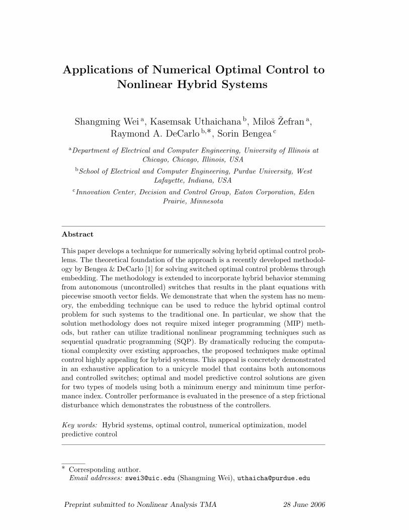
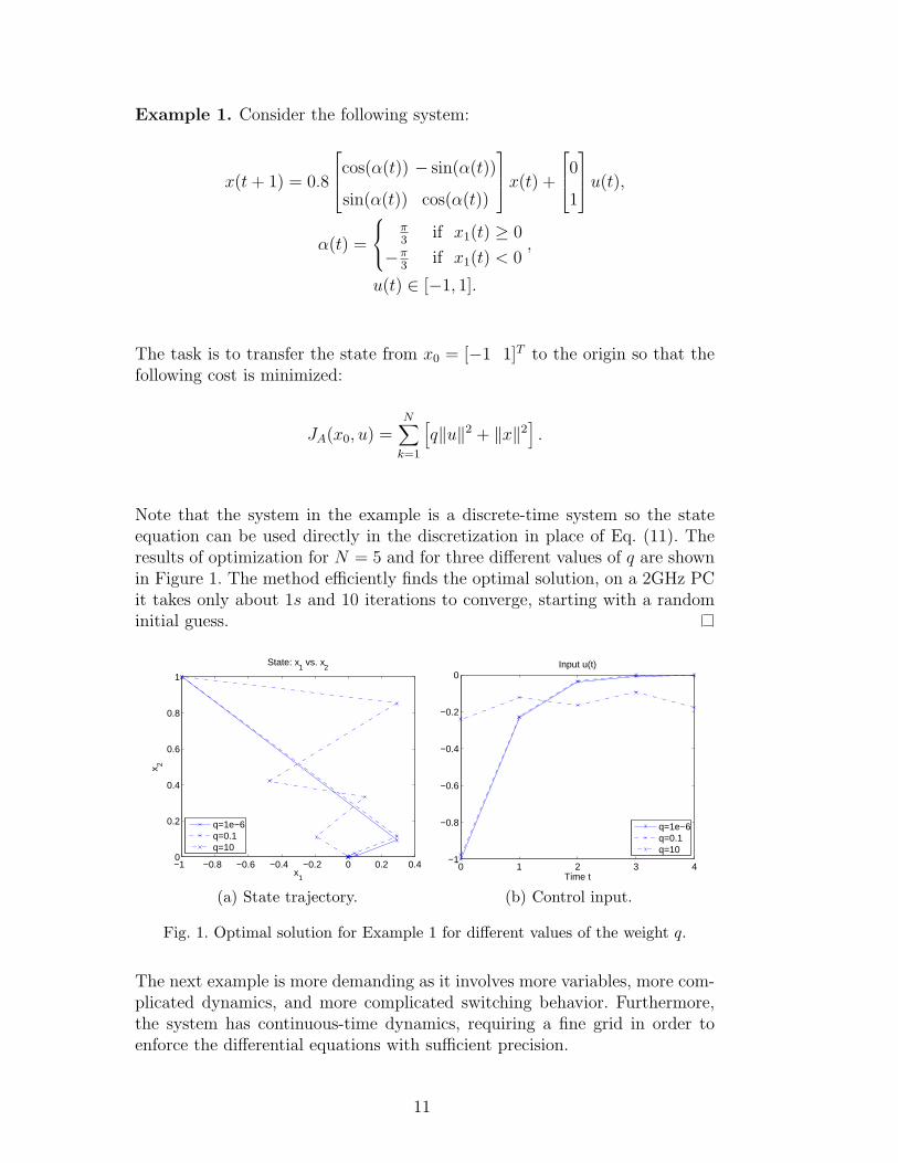
Note that the system in the example is a discrete-time system so the stateequation can be used directly in the discretization in place of Eq. (11). Theresults of optimization for N = 5 and for three different values of q are shownin Figure 1. The method efficiently finds the optimal solution, on a 2GHz PCit takes only about 1s and 10 iterations to converge, starting with a randominitial guess.

−1 −0.8 −0.6 −0.4 −0.2 0 0.2 0.40

0.2

0.4

0.6

0.8

1

x1

x 2

State: x1 vs. x

2

q=1e−6q=0.1q=10

(a) State trajectory.

0 1 2 3 4−1

−0.8

−0.6

−0.4

−0.2

0

Time t

Input u(t)

q=1e−6q=0.1q=10

(b) Control input.

Fig. 1. Optimal solution for Example 1 for different values of the weight q.

The next example is more demanding as it involves more variables, more com-plicated dynamics, and more complicated switching behavior. Furthermore,the system has continuous-time dynamics, requiring a fine grid in order toenforce the differential equations with sufficient precision.

11

Example 2. Consider the following system with 4 states and 2 inputs:

x(t) =

A1x(t) 9 < x21 + x2

2 + ‖u‖2 ≤ 100

A2x(t) +B2u(t) otherwise,

where

A1 =

0 0 1 0

0 0 0 1

1 0 0 0

0 1 0 0

A2 =

0 0 1 0

0 0 0 1

0 0 0 0

0 0 0 0

B2 =

0 0

0 0

1 0

0 1

.

The task is to bring the system to the origin in 1s so that the following costfunctional is minimized:

JA(x0, u) =∫ 1

0‖u‖2dt.

It is worth noting that the surface on which the system switches is nonlinearand it depends both on the state and the input. The system can be interpretedas a model for a mass particle sliding on a horizontal plane and controlled bytwo thrusters. The particle has to pass through a repulsive region where thethrusters have no effect on the motion before approaching the origin.

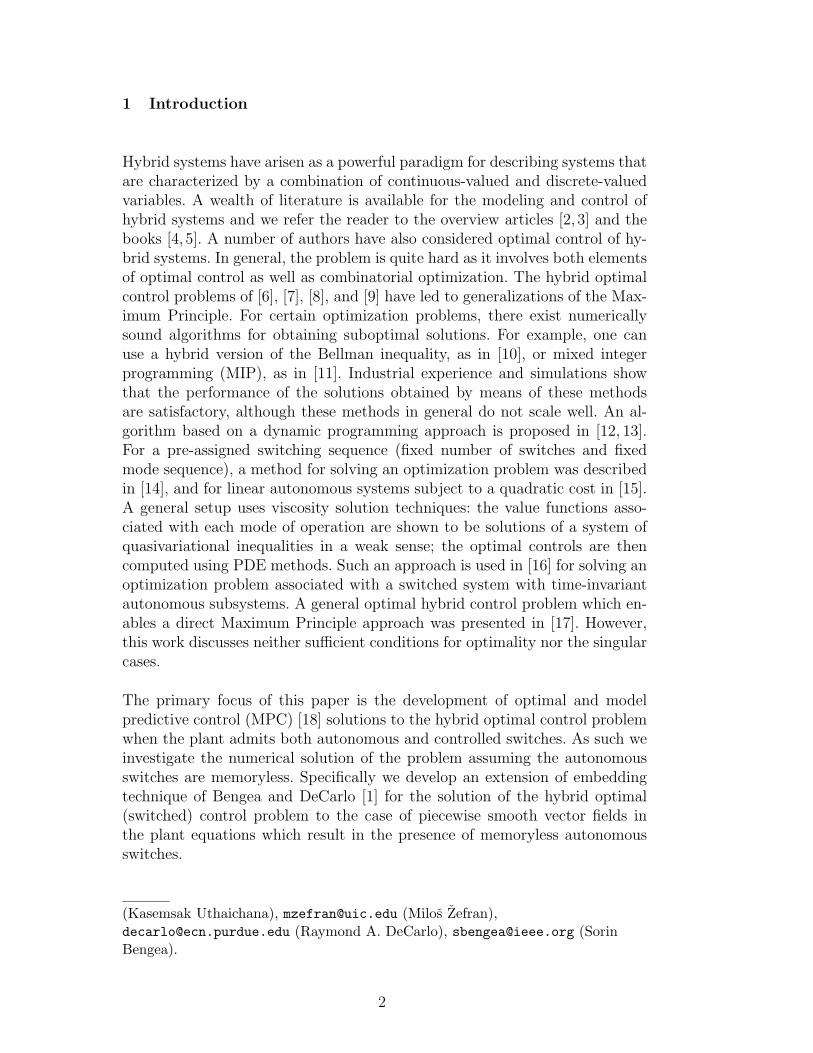
For the computation, we chose to discretize the system on a uniform grid with100 points. Due to a large number of variables the optimization took around10 minutes to converge on a 2GHz PC. We started with a random initial guessand computed the optimal solution on a grid with 10 points. This solution wassubsequently used as the initial guess for a grid with 20, 40, and finally 100points, the solution from each step serving as the initial guess for the next.

0 0.2 0.4 0.6 0.8 1−15

−10

−5

0

5

10

15

20

Time t

State x(t)

x

1

x2

x3

x4

(a) State trajectory.

0 0.2 0.4 0.6 0.8 1−80

−60

−40

−20

0

20

40

60

80

Time t

Input u(t)

u

1u

2

Mode

(b) Control input.

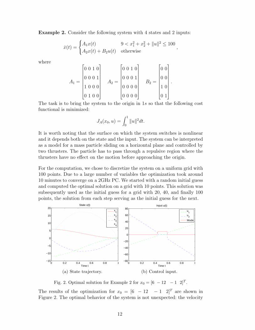
Fig. 2. Optimal solution for Example 2 for x0 = [6 − 12 − 1 2]T .

The results of the optimization for x0 = [6 − 12 − 1 2]T are shown inFigure 2. The optimal behavior of the system is not unexpected: the velocity

12

of the mass particle is increased before entering the repulsive region so thatthe particle can slide through it. In the repulsive region the thrusters haveno effect so they are turned off to reduce the cost. After the particle leavesthe repulsive region, the thrusters become active and bring the particle to theorigin.

5.2 Decoupled switches: Unicycle Application

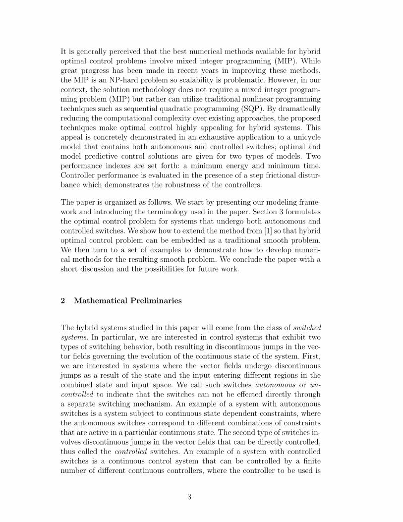
To demonstrate the full power of the approach in Section 3 we will showhow to compute optimal trajectories for a system exhibiting both controlledand autonomous switches. The example we will use is a unicycle driving on ahorizontal plane (Figure 3). The wheel of the unicycle can either roll or slide,resulting in autonomous switches. In addition, we assume that the unicyclehas a regenerative brake that can be turned on or off. These switches arecontrolled. We will consider two different models of the unicycle. The firstmodel is for the unicycle with a separate motor and a generator both connectedto a battery-pack; the other model assumes that the unicycle contains onlyone electric drive-battery-pack that performs as either a motor or a generator.The essential features of each model are listed in Table 1 which also indicatesthe designated modes.

Table 1Characteristics of the two modelsQuantities Model A Model B

Number of electric machines 2 1

Mode-1 denotation Brake-off Propelling

Mode-2 denotation Brake-on Regenerative Braking

Torque u1 in Mode-1 Propelling and Propelling Torque Only

Braking Torque

Referring to Figure 3, the forward velocity of the wheel is controlled by thetorque u1, while its heading is controlled by the torque u2. Our objective is toformulate and solve two hybrid optimal control problems: (i) drive the unicycleto the origin within an allotted time while minimizing weighted power usageand (ii) drive the unicycle from the same initial condition as in problem (i) tothe origin in minimum time. As discussed earlier, we will use model predictivecontrol (MPC) [18] to compute the control inputs for the embedded system.

13

1 u

m

r

x

y

2 u

x v y v

h

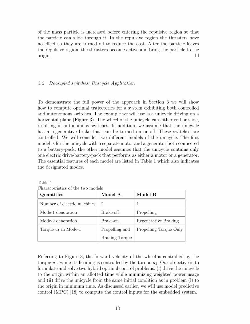
Fig. 3. A top view and a side view of the unicycle

5.2.1 Unicycle Model

The generalized coordinates for the unicycle are its center of mass position xand y, body orientation θ (heading) relative to the x-axis, and the rotation ofthe wheel φ. Since we are not interested in φ itself, the state variables for thesystem are zT = [x, y, θ, vx, vy, θ, φ]T ∈ R7, where [vx, vy] is the velocity of thecenter of mass of the unicycle, expressed in the body frame, θ is the turningvelocity of the unicycle, and φ is the angular velocity of the wheel as it spinson its axle. For either model the equations of motion for the unicycle take theform:

x = vx cos(θ)− vy sin(θ),

y = vx sin(θ) + vy cos(θ),

θ = θ,

vx =Fx(z)

m+ θvy,

vy =Fy(z)

m− θvx,

θ =1

I2u2,

φ =Fxr

I1+

1

I1u1,

(12)

where(i) m is the mass of the unicycle, (ii) r is the radius of the wheel, (iii) I1is the moment of inertia of the wheel around its axis, (iv) I2 is the moment ofinertia of the unicycle about the vertical axis through the center of mass, and(v) Fx and Fy are the forces between the ground and the wheel in the forwardand lateral directions, respectively. As discussed above, u1 is the control torqueapplied to the axle of the wheel, while u2 is the torque controlling the headingof the unicycle. The structure of u1 will differentiate the model types and isdescribed later.

The distinctive hybrid nature of the unicycle occurs because the forces Fx(z)and Fy(z) depend on whether the unicycle is rolling or sliding. In the rolling

14

mode, the relative velocity vr , [vrx, vry]T = [vx+φr, vy]

T , between the groundand the wheel’s point of contact is zero, i.e.,

vrx = vx + φr = 0,

vry = vy = 0.(13)

From Eqs. (13) and (12) we have that

Fx(z) = − mru1

mr2 + I1Fy(z) = −mrθφ.

(14)

Here, the forces Fx(z) and Fy(z) are ground reaction forces that prevent wheelslippage. In the sliding mode, Fx(z) and Fy(z) are frictional forces. In summarythe forces Fx and Fy are given by the following expressions

Fx(z) =

−mru1

mr2+I1rolling mode

−µdvx+φr‖vr‖ mg sliding mode

(15)

Fy(z) =

−mrθφ rolling mode

−µdvy

‖vr‖mg sliding mode(16)

where µd is the coefficient of dynamic friction and g is the gravitational con-stant.

The autonomous switch from rolling to sliding occurs when the magnitude ofthe constraint force F , [Fx, Fy]

T exceeds the maximum possible magnitudeof the static friction, µsmg , i.e.,

‖F‖ > µsmg ⇒ rolling → sliding, (17)

where µs is the coefficient of static friction. On the other hand, the switchfrom sliding to rolling occurs when (i) vr = [vrx, vry]

T = 0 , and (ii) themaximum magnitude of the frictional force exceeds that of the constraintforce F = [Fx, Fy]

T , i.e.,

‖vr‖ = 0 and ‖F‖ 6 Fs,max = µsmg ⇒ sliding → rolling. (18)

Therefore, the system has two kinds of switches:

(1) Autonomous switches where the system switches between rolling and slid-ing depending on the physics of the contact.

(2) Controlled switches where the regenerative brake can be switched on oroff arbitrarily.

Let Model A denote the configuration of a separate motor and generator.

15

Mode 1 will denote the use of

u1 = u11A ∈ [−20, 20] (19)

as an actuating torque that can be either propelling or braking. Mode 2 denotesthe use of regenerative braking alone in which case

u1 = u21A =

−Kbφ,∣∣∣φ∣∣∣ 6 2

−20 sgn(φ),∣∣∣φ∣∣∣ > 2

(20)

whereKb = 10 is a fixed regenerative braking coefficient; note that u1 saturatesat 20Nm.

Let Model B denote the configuration of a single electric drive that can operateeither as a (propelling) motor or as a generator for regenerative braking. Formodel B, the control input

u1 = u11B(t) sgn(φ)umax

1 (21)

strictly provides propelling torque in Mode 1, where umax1 = 20Nm, u1

1B(t) ∈[0, 1] modulates umax

1 , and sgn(φ) insures that the applied torque is alwayspropelling. The regenerative braking term for Mode 2 coincides with thatused for Model A, i.e.,

u1 = u21B =

−Kbφ,∣∣∣φ∣∣∣ 6 2

−20 sgn(φ),∣∣∣φ∣∣∣ > 2

(22)

Note that for each model, Modes 1 and 2 are possible in both the rolling andsliding modes. For each model the unicycle is thus an example of a systemwith decoupled switches given by Eq. (2).

5.2.2 Embedded Model Formulation

We now follow the procedure outlined in Section 3.2. For simplicity, let v1 = αand v2 = 1− α and define for both models

u1(t) = (1− α(t))u11(t) + α(t)u2

1(t) (23)

The variable α(t) ∈ 0, 1 denotes the original problem whereas α(t) ∈ [0, 1]denotes the embedded problem which will be solved in this investigation. Thus,the embedded formulation is given by Eqs. (12) and (23) with the specificstructures of Eqs. (19)-(22) from Models A and B respectively and the forcesFx(z), and Fy(z) of the unicycle motion in rolling and sliding given by Eqs. (15)and (16) respectively. Because of the autonomous switches determined byEqs. (17) and (18), the right hand side of Eq. (12) is piecewise continuous

16

provided the system does not chatter about the boundary implicitly definedby Eqs. (17) and (18) 4 .

5.2.3 The Performance Index and MPC Design

5.2.3.1 Fixed Time Control. The first objective of the control designfor each model is to drive the unicycle from a given starting initial state, zT

0 =[x(0), y(0), θ(0), vx(0), vy(0), θ(0), φ(0)]T back to the origin while minimizingthe energy usage. In addition, since sliding of the wheel is undesirable since itimplies the loss of controllability, we would like to limit the sliding motion ofthe unicycle. Hence, the integral performance index for this study is taken as

J = c0 ‖z(T )‖2 +∫ T

0

[c1 (1− α)u2

1 + c2u22 + c3‖vr‖2

]dt (24)

where the positive weights ci (for i = 0, . . . , 4) are constant. The term (i)c0 ‖z(T )‖2 drives the final states of the unicycle z(T ) toward the origin; (ii)c1 (1− α)u2

1 penalizes the actuating power usage; (iii) c2u22 penalizes the head-

ing power usage; and (iv) c3‖vr‖2 is to limit sliding motion. The terminal con-straints are enforced through the cost functional (as soft constraints) ratherthan imposed as hard constraints because the system is stabilizable but notcontrollable in the sliding regime. Therefore, using hard constraints could makethe optimal control problem unfeasible. Note also that there is no penalty forregenerative braking usage.

The first objective thus leads to minimization of the performance index inEq. (24) subject to the embedded state dynamics given by Eqs. (12)-(23) andan initial state z0, resulting in an optimal control input for the nominal dy-namical system. However, when applying the computed controls to the actualmodel that differs from the nominal model due to the presence of distur-bances or modeling uncertainties, the state trajectory might deviate from thedesired trajectory, and fail to reach the desired final state within the allottedtime interval. To cope with such disturbances and uncertainties, an MPC-type controller that is well-known for its robustness will be adopted to drivethe unicycle from a given initial state z0 to the origin at a pre-specified finaltime. The adopted optimal control based MPC approach can be summarizedin steps as follows:

(1) Given z0, partition the time interval T into N equal subintervals of lengthh = T

N, for the purpose of computing a (backward) piecewise constant

control sequence u1, . . . , uN, where ui =[u1(ih) u2(ih)

]T

, and the

state values z1, . . . , zN.4 An analysis of the vector fields on the switching surface shows that chatteringcan not occur.

17

(2) For k = 1, . . . , N , solve the embedded problem of the unicycle over thereceding horizon [k,N ] by minimizing the performance index given byEq. (24) subject to the nominal model with the initial state zk−1 andobtain the (look ahead) control sequence uk, . . . , uN.

(3) Apply the control input uk for the time interval tk−1 ≤ t < tk to the realmodel. The value of the state of the real model at the end of the intervalbecomes zk, the initial condition for the next iteration.

(4) Repeat steps 2 and 3 until k = N .

A variation of the direct collocation method from Section 4 is used to numer-ically solve the embedded optimal control problem at each step of the MPCalgorithm. As per development in Section 4, the discretized control input isassumed to be piecewise constant function:

u(t) = u(tj), tj ≤ t < tj+1, i = 0, . . . , N − 1.

However, unlike in Section 4, since the switching between sliding and rollingrequires precise solution of the state equations, the state equations are inte-grated directly for the given control variables using Runga-Kutta ODE solver.

5.2.3.2 Time Optimal Control. The second objective of this work isthe construction of a minimum time control. Given the same initial point,zT0 = [x(0), y(0), vx(0), vy(0), θ(0), θ(0), φ(0)]T , drive the state to the origin in

minimum time. The performance index in this case is

J = c0 ‖z(tf )‖2 +

tf∫0

1dt, (25)

where c0 = 2 · 104 and tf is the unknown final time. As before, the terminalstate constraint is soft in that we only penalize the deviation from the origin.

Controller construction entails a discretization which cannot be done directlysince the final time is unknown. By letting t = tfs, an equivalent version ofperformance index (25) is obtained as

minu,α,tf

c0 ‖z(1)‖2 +

1∫0

tf ds (26)

where s ∈ [0, 1] is normalized time and tf is an unknown constant. With thisformulation the same method as above can be used to solve the optimizationproblem.

Some variation is needed for the MPC strategy. Initially, the interval [0, 1] ispartitioned into N subintervals of width h = 1

N. After computing u1, . . . , uN

18

−3 −2 −1 0 1 2 30

0.5

1

1.5

2

2.5

3

3.5

4

x

y

x−y trajectories

ActualNominalSlippery Area

(a) Wheel’s position on x-y plane

0 0.1 0.2 0.3 0.4 0.5 0.6 0.7 0.8 0.9 1−1.5

−1

−0.5

0

Normalized time t/T (T=9.5s)

vx and v

y

vx Actual

vy Actual

vx Nominal

vy Nominal

(b) Forward and lateral velocities

0 0.1 0.2 0.3 0.4 0.5 0.6 0.7 0.8 0.9 1Normalized time t/T (T=9.5s)

Mode

Brake on/off ActualRolling/sliding ActualBrake on/off NominalRolling/sliding Nominal

on

off

rolling

sliding

(c) Modes of operation

0 0.1 0.2 0.3 0.4 0.5 0.6 0.7 0.8 0.9 1−20

−15

−10

−5

0

5

10

15

20

Normalized time t/T (T=9.5s)

Control Torques

u1 Actualu2 Actualu1 Nominalu2 Nominal

(d) Control inputs

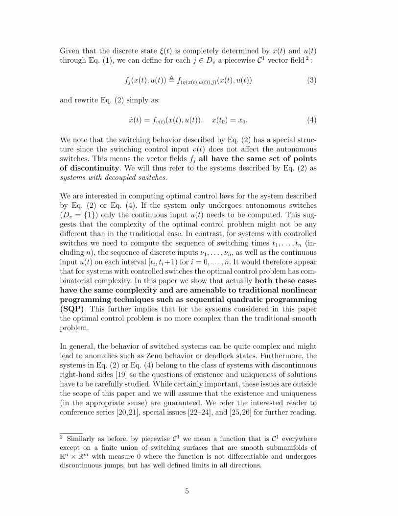
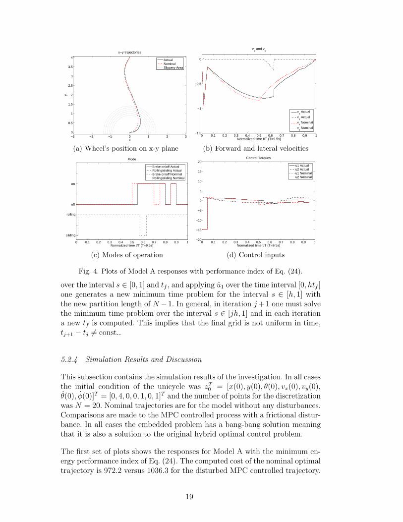
Fig. 4. Plots of Model A responses with performance index of Eq. (24).

over the interval s ∈ [0, 1] and tf , and applying u1 over the time interval [0, htf ]one generates a new minimum time problem for the interval s ∈ [h, 1] withthe new partition length of N −1. In general, in iteration j+1 one must solvethe minimum time problem over the interval s ∈ [jh, 1] and in each iterationa new tf is computed. This implies that the final grid is not uniform in time,tj+1 − tj 6= const..

5.2.4 Simulation Results and Discussion

This subsection contains the simulation results of the investigation. In all casesthe initial condition of the unicycle was zT

0 = [x(0), y(0), θ(0), vx(0), vy(0),θ(0), φ(0)]T = [0, 4, 0, 0, 1, 0, 1]T and the number of points for the discretizationwas N = 20. Nominal trajectories are for the model without any disturbances.Comparisons are made to the MPC controlled process with a frictional distur-bance. In all cases the embedded problem has a bang-bang solution meaningthat it is also a solution to the original hybrid optimal control problem.

The first set of plots shows the responses for Model A with the minimum en-ergy performance index of Eq. (24). The computed cost of the nominal optimaltrajectory is 972.2 versus 1036.3 for the disturbed MPC controlled trajectory.

19

The nominal response is for the model without disturbances whereas the MPCcontrol is for the frictional disturbance where in an annulus 0.9 6 r 6 1.4around the origin the static coefficient of friction µs drops from 0.7 to 0.002,and the dynamic coefficient of friction µd drops from 0.6 to 0.001. Moreover,the unicycle’s nominal parameters mnominal = 1 and rnominal = 4 during thesimulation were perturbed so that mactual = 1.05 and ractual = 3.9. Afterstarting in the sliding mode, the unicycle is driven to the rolling mode afterabout 0.2s. At around 5s the unicycle encounters the frictional disturbancesand switches from rolling to sliding as indicated in Figure 4(c). However, af-ter leaving the slippery area at about 6s, in conjunction with the correctiveaction of the MPC controller, the unicycle starts to roll again. Figure 4(a)and Figure 4(b) show the unicycle’s trajectories and the evolutions of twostates vx and vy. It clearly shows that the unicycle can still reach the ori-gin in the required time despite disturbances and model errors. Figure 4(d)displays the control inputs which again adapt in accordance with state andmodel changes. The results thus confirm that the influence of disturbances onsystem performance is small and the MPC scheme achieves good performanceand robustness. Recall that for this model, the electric motor can apply botha propelling torque and a braking torque u1

1 in Mode 1, while a regenerativebraking torque u2

1 is applied in Mode 2. One observes that during the final 4sof the simulation, the switches of the braking torque in Mode 1 and the re-generative braking torque in Mode 2 are coordinated to reduce cost and reachthe origin on time.

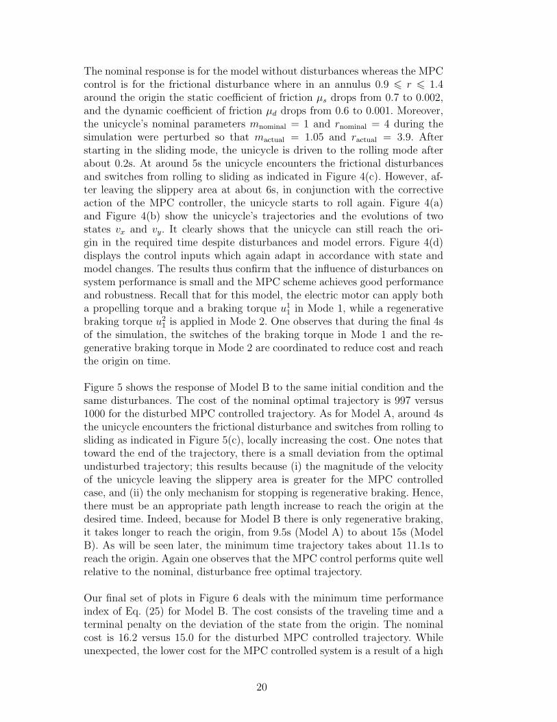
Figure 5 shows the response of Model B to the same initial condition and thesame disturbances. The cost of the nominal optimal trajectory is 997 versus1000 for the disturbed MPC controlled trajectory. As for Model A, around 4sthe unicycle encounters the frictional disturbance and switches from rolling tosliding as indicated in Figure 5(c), locally increasing the cost. One notes thattoward the end of the trajectory, there is a small deviation from the optimalundisturbed trajectory; this results because (i) the magnitude of the velocityof the unicycle leaving the slippery area is greater for the MPC controlledcase, and (ii) the only mechanism for stopping is regenerative braking. Hence,there must be an appropriate path length increase to reach the origin at thedesired time. Indeed, because for Model B there is only regenerative braking,it takes longer to reach the origin, from 9.5s (Model A) to about 15s (ModelB). As will be seen later, the minimum time trajectory takes about 11.1s toreach the origin. Again one observes that the MPC control performs quite wellrelative to the nominal, disturbance free optimal trajectory.

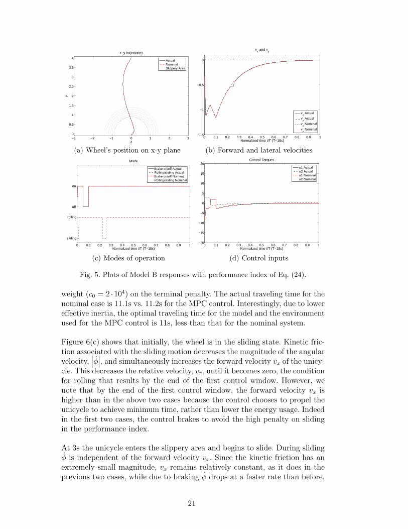
Our final set of plots in Figure 6 deals with the minimum time performanceindex of Eq. (25) for Model B. The cost consists of the traveling time and aterminal penalty on the deviation of the state from the origin. The nominalcost is 16.2 versus 15.0 for the disturbed MPC controlled trajectory. Whileunexpected, the lower cost for the MPC controlled system is a result of a high

20

−3 −2 −1 0 1 2 30

0.5

1

1.5

2

2.5

3

3.5

4

x

y

x−y trajectories

ActualNominalSlippery Area

(a) Wheel’s position on x-y plane

0 0.1 0.2 0.3 0.4 0.5 0.6 0.7 0.8 0.9 1−1.5

−1

−0.5

0

Normalized time t/T (T=15s)

vx and v

y

vx Actual

vy Actual

vx Nominal

vy Nominal

(b) Forward and lateral velocities

0 0.1 0.2 0.3 0.4 0.5 0.6 0.7 0.8 0.9 1Normalized time t/T (T=15s)

Mode

Brake on/off ActualRolling/sliding ActualBrake on/off NominalRolling/sliding Nominal

on

off

sliding

rolling

(c) Modes of operation

0 0.1 0.2 0.3 0.4 0.5 0.6 0.7 0.8 0.9 1−20

−15

−10

−5

0

5

10

15

20

Normalized time t/T (T=15s)

Control Torques

u1 Actualu2 Actualu1 Nominalu2 Nominal

(d) Control inputs

Fig. 5. Plots of Model B responses with performance index of Eq. (24).

weight (c0 = 2 ·104) on the terminal penalty. The actual traveling time for thenominal case is 11.1s vs. 11.2s for the MPC control. Interestingly, due to lowereffective inertia, the optimal traveling time for the model and the environmentused for the MPC control is 11s, less than that for the nominal system.

Figure 6(c) shows that initially, the wheel is in the sliding state. Kinetic fric-tion associated with the sliding motion decreases the magnitude of the angularvelocity,

∣∣∣φ∣∣∣, and simultaneously increases the forward velocity vx of the unicy-cle. This decreases the relative velocity, vr, until it becomes zero, the conditionfor rolling that results by the end of the first control window. However, wenote that by the end of the first control window, the forward velocity vx ishigher than in the above two cases because the control chooses to propel theunicycle to achieve minimum time, rather than lower the energy usage. Indeedin the first two cases, the control brakes to avoid the high penalty on slidingin the performance index.

At 3s the unicycle enters the slippery area and begins to slide. During slidingφ is independent of the forward velocity vx. Since the kinetic friction has anextremely small magnitude, vx remains relatively constant, as it does in theprevious two cases, while due to braking φ drops at a faster rate than before.

21

−3 −2 −1 0 1 2 30

0.5

1

1.5

2

2.5

3

3.5

4

x

y

x−y trajectories

ActualNominalSlippery Area

(a) Wheel’s position on x-y plane

0 0.1 0.2 0.3 0.4 0.5 0.6 0.7 0.8 0.9 1−1.5

−1

−0.5

0

Normalized time t/T (T=11.1s)

vx and v

y

vx Actual

vy Actual

vx Nominal

vy Nominal

(b) Forward and lateral velocities

0 0.1 0.2 0.3 0.4 0.5 0.6 0.7 0.8 0.9 1Normalized time t/T (T=11.1s)

Mode

Brake on/off ActualRolling/sliding ActualBrake on/off NominalRolling/sliding Nominal

on

off

rolling

sliding

(c) Modes of operation

0 0.1 0.2 0.3 0.4 0.5 0.6 0.7 0.8 0.9 1−20

−15

−10

−5

0

5

10

15

20

Normalized time t/T (T=11.1s)

Control Torques

u1 Actualu2 Actualu1 Nominalu2 Nominal

(d) Control inputs

Fig. 6. Simulation results for minimum time problem of Model B

Finally, faced with the longer path in addition to the (soft) terminal constraint,the MPC makes a ”no cost” abrupt change in the steering wheel during thelast few control windows to achieve the terminal constraint. Indeed, the MPCcontrol which uses a receding horizon is more sensitive to the terminal con-straint during the last few control windows as seen in Eq. (26).

6 Conclusion

The paper studies applications of numerical optimal control to nonlinear hy-brid systems. While the formulation of the optimal control problem for hybridsystems depends on the nature of the mode switches of the system, we showthat in contrast to a widely accepted belief that such problems always lead tomixed integer programming problems (MIPs), in many important cases tra-ditional nonlinear programming techniques such as sequential quadratic pro-gramming (SQP) can be readily applied. In particular, we demonstrate thatwhen the switches are autonomous (uncontrolled) the optimal control prob-lem can be solved using traditional techniques. Furthermore, while controlledswitches can possibly lead to a combinatorial complexity of the numerical al-

22

gorithms, we show that an extension of techniques recently developed in [1]can again effectively reduce such problems to the traditional one. By dramat-ically reducing the computational complexity over existing approaches, theproposed techniques make optimal control highly appealing for hybrid sys-tems, potentially leading to a much broader appeal of hybrid system models.As an application, we show in detail how the proposed techniques can beapplied to a unicycle model that contains both autonomous and controlledswitches.

Acknowledgment

The authors thank Dr. Michael Branicky for his comments on an earlier versionof this paper. The work of S. Wei and M. Zefran has been supported in partby NSF grants IIS-0093581 and CCR-0330342.

References

[1] S. C. Bengea, R. A. DeCarlo, Optimal control of switching systems, AutomaticaJ. IFAC 41 (1) (2005) 11–27.

[2] R. A. Decarlo, M. S. Branicky, S. Pettersson, B. Lennartson, Perspectives andresults on the stability and stabilizability of hybrid systems, Proceedings of theIEEE 88 (7) (2000) 1069–1082.

[3] R. Alur, T. Henzinger, G. Lafferriere, G. Pappas, Discrete abstractions of hybridsystems, Proceedings of the IEEE 88 (7) (2000) 971–984.

[4] A. J. van der Schaft, J. M. Schumacher, An Introduction to Hybrid DynamicalSystems, Vol. 251 of Lecture Notes in Control and Information Sciences,Springer Verlag, 1999.

[5] D. Liberzon, Switching in Systems and Control, Birkhauser, Boston, MA, 2003.

[6] M. S. Branicky, V. S. Borkar, S. K. Mitter, A unified framework for hybridcontrol: model and optimal control theory, IEEE Transactions on AutomaticControl 43 (1) (1998) 31–45.

[7] C. G. Cassandras, D. L. Pepyne, Y. Wardi, Optimal control of a class of hybridsystems, IEEE Transactions on Automatic Control 46 (3) (2001) 398–415.

[8] B. M. Miller, E. Y. Rubinovich, Impulsive control in continuous and discrete-continuous systems, Kluwer Academic/Plenum Publishers, New York, 2003.

[9] H. J. Sussmann, A maximum principle for hybrid optimal control problems, in:IEEE Conf. on Decision and Control, Phoenix, AZ, USA, 1999, pp. 425–430.

23

[10] S. Hedlund, A. Rantzer, Optimal control of hybrid systems, in: IEEE Conf.on Decision and Control, Vol. 4 of Proceedings of the IEEE Conference onDecision and Control, IEEE, Piscataway, NJ, USA, Phoenix, AZ, USA, 1999,pp. 3972–3977.

[11] A. Bemporad, M. Morari, Control of systems integrating logic, dynamics, andconstraints, Automatica 35 (3) (1999) 407–427.

[12] X. Xu, P. J. Antsaklis, A dynamic programming approach for optimal controlof switched systems, in: IEEE Conf. on Decision and Control, Sydney, NSW,2000, pp. 1822–1827.

[13] X. Xu, P. J. Antsaklis, Results and perspectives on computational methods foroptimal control of switched systems, in: Proc. Hybrid Systems: Computationand Control, HSCC 2003, Vol. 2623 of Lecture Notes in Computer Science,Springer-Verlag, Prague, Czech Republic, 2003, pp. 540–556.

[14] M. Zefran, J. Desai, V. Kumar, Continuous motion plans for robotic systemswith changing dynamic behavior, proceedings of 2nd Int. Workshop onAlgorithmic Foundations of Robotics (1996).

[15] A. Giua, C. Seatzu, C. Van Der Mee, Optimal control of switched autonomouslinear systems, in: IEEE Conf. on Decision and Control, Vol. 3, Orlando, FL,2001, pp. 2472–2477.

[16] I. Capuzzo-Dolcetta, L. C. Evans, Optimal switching for ordinary differentialequations, SIAM Journal of Control and Optimization 22 (1) (1984) 143–161.

[17] P. Riedinger, C. Zanne, F. Kratz, Time optimal control of hybrid systems, in:American Control Conference, San Diego, CA, 1999, pp. 2466–2470.

[18] E. F. Camacho, C. Bordons, Model Predictive Control, Springer Verlag, 2004.

[19] A. F. Filippov, Differential equations with discontinuous right–hand sides, AMSTranslations, Ser. 2 42 (1964) 199–231.

[20] P. Antsaklis, W. Kohn, A. Nerode, S. S. Sastry (Eds.), Hybrid systems IV, Vol.1273 of Lecture notes in computer science, Springer Verlag, New York, NY,1997.

[21] F. W. Vaandrager, J. H. van Schuppen (Eds.), Hybrid systems: Computationand control, Vol. 1596 of Lecture notes in computer science, Springer Verlag,New York, NY, 1999.

[22] P. Antsaklis, A. Nerode (Eds.), Special issue on Hybrid systems, Vol. 43 of IEEETransactions on Automatic Control, 1998.

[23] A. Morse, C. Pantelides, S. Sastry, , J. Schumacher (Eds.), Special issue onHybrid systems, Vol. 35 of Automatica, 2000.

[24] P. Antsaklis (Ed.), Special issue on Hybrid systems, Vol. 88 of Proceedings ofthe IEEE, 2000.

24

[25] J. Imura, A. van der Schaft, Characterization of well-posedness of piecewise-linear systems, IEEE Transactions on Automatic Control 45 (9) (2000) 1600–1619.

[26] J. L. K. Johansson, S. Simic, J. Zhang, S. Sastry, Dynamical properties of hybridautomata, IEEE Transactions on Automatic Control 48 (1) (2003) 2–17.

[27] P. Riedinger, F. Kratz, C. Iung, C. Zanne, Linear quadratic optimization forhybrid systems, in: IEEE Conf. on Decision and Control, Phoenix, AZ, 1999,pp. 3059–3064.

[28] L. D. Berkovitz, Optimal control theory, Springer Verlag, New York, NY, 1974.

[29] A. M. Cervantes, L. T. Biegler, Optimization strategies for dynamic systems,in: C. Floudas, P. Pardalos (Eds.), Encyclopedia of Optimization, Kluwer, 2001,pp. 216–227.

[30] O. von Stryk, R. Bulirsch, Direct and indirect methods for trajectoryoptimization, Ann. Oper. Res. 37 (1-4) (1992) 357–373, nonlinear methods ineconomic dynamics and optimal control (Vienna, 1990).

[31] O. von Stryk, Numerical solution of optimal control problems by directcollocation, in: Optimal control (Freiburg, 1991), Vol. 111 of Internat. Ser.Numer. Math., Birkhauser, Basel, 1993, pp. 129–143.

25