optimal load management application for industrial consumers · je erson fabricio ord onez~ gir on...

Optimal Load ManagementApplication for Industrial Customers

by

Jefferson Fabricio Ordonez Giron

A thesispresented to the University of Waterloo

in fulfillment of thethesis requirement for the degree of

Master of Applied Sciencein

Electrical and Computer Engineering

Waterloo, Ontario, Canada, 2015

c© Jefferson Fabricio Ordonez Giron 2015

I hereby declare that I am the sole author of this thesis. This is a true copy of the thesis,including any required final revisions, as accepted by my examiners.

I understand that my thesis may be made electronically available to the public.

ii

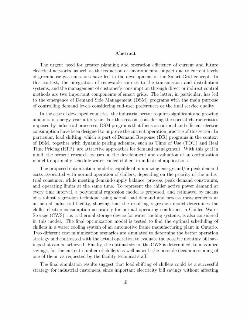
Abstract

The urgent need for greater planning and operation efficiency of current and futureelectrical networks, as well as the reduction of environmental impact due to current levelsof greenhouse gas emissions have led to the development of the Smart Grid concept. Inthis context, the integration of renewable sources to the transmission and distributionsystems, and the management of customer’s consumption through direct or indirect controlmethods are two important components of smart grids. The latter, in particular, has ledto the emergence of Demand Side Management (DSM) programs with the main purposeof controlling demand levels considering end-user preferences or the final service quality.

In the case of developed countries, the industrial sector requires significant and growingamounts of energy year after year. For this reason, considering the special characteristicsimposed by industrial processes, DSM programs that focus on rational and efficient electricconsumption have been designed to improve the current operation practice of this sector. Inparticular, load shifting, which is part of Demand Response (DR) programs in the contextof DSM, together with dynamic pricing schemes, such as Time of Use (TOU) and RealTime Pricing (RTP), are attractive approaches for demand management. With this goal inmind, the present research focuses on the development and evaluation of an optimizationmodel to optimally schedule water-cooled chillers in industrial applications.

The proposed optimization model is capable of minimizing energy and/or peak demandcosts associated with normal operation of chillers, depending on the priority of the indus-trial consumer, while meeting demand-supply balance, process, peak demand constraints,and operating limits at the same time. To represent the chiller active power demand atevery time interval, a polynomial regression model is proposed, and estimated by meansof a robust regression technique using actual load demand and process measurements atan actual industrial facility, showing that the resulting regression model determines thechiller electric consumption accurately for normal operating conditions; a Chilled WaterStorage (CWS), i.e. a thermal storage device for water cooling systems, is also consideredin this model. The final optimization model is tested to find the optimal scheduling ofchillers in a water cooling system of an automotive frame manufacturing plant in Ontario.Two different cost minimization scenarios are simulated to determine the better operationstrategy and contrasted with the actual operation to evaluate the possible monthly bill sav-ings that can be achieved. Finally, the optimal size of the CWS is determined, to maximizesavings, for the current number of chillers as well as with the possible decommissioning ofone of them, as requested by the facility technical staff.

The final simulation results suggest that load shifting of chillers could be a successfulstrategy for industrial customers, since important electricity bill savings without affecting

iii

the normal plant operation were attained. This was possible due to an optimal chillerscheduling and indirect incentives provided by current industry energy price schemes inOntario. Furthermore, the optimization model presented permitted to optimally size theCWS in the water cooling system studied, so that electricity costs were minimized de-pending on the total chiller capacity considered. Therefore, optimization approaches toschedule industrial processes could be a powerful tool to increase the operational efficiencyof industrial plants to reduce their significant energy costs.

iv

Acknowledgements

I would like to acknowledge and thank all the invaluable support of my supervisorProfessor Claudio Canizares. His patience and guidance were always inspirational to carryout this research.

My deepest gratitude to Professor Kankar Bhattacharya and Professor Mehrdad Kaz-erani for their insightful comments that helped to improve the final content of this thesis.

Of course, I cannot forget all the interesting moments and discussions with my friendsMauricio, Daniel, Dario, Bharat, Shubha, Juan Carlos, Mariano, Gabriel, Mostafa, Amir,Behnam, Nafeesa, Alfredo, and Doug. Thank you all for your friendship and camaraderieduring these two years in Waterloo. All the best for you ever.

I would like to thank Nelson, Rocio and their family for helping my wife and I fromthe very beginning. Away from home, they always made their best to make us feel a bitcloser to Ecuador.

My special acknowledgment to SENESCYT for providing the necessary funding tocomplete my grad studies.

v

Dedication

I could not have finished this journey without the support of my beloved wife Mayraand my family. Thanks for being all in my life.

vi

Table of Contents

List of Tables ix

List of Figures x

List of Acronyms xii

Nomenclature xiv

1 Introduction 1

1.1 Motivation . . . . . . . . . . . . . . . . . . . . . . . . . . . . . . . . . . . . 1

1.2 Literature Review . . . . . . . . . . . . . . . . . . . . . . . . . . . . . . . . 3

1.2.1 Load Management . . . . . . . . . . . . . . . . . . . . . . . . . . . 3

1.2.2 Optimal Load Management . . . . . . . . . . . . . . . . . . . . . . 4

1.3 Objectives . . . . . . . . . . . . . . . . . . . . . . . . . . . . . . . . . . . . 6

1.4 Contents . . . . . . . . . . . . . . . . . . . . . . . . . . . . . . . . . . . . . 7

2 Background 9

2.1 Demand Side Management (DSM) . . . . . . . . . . . . . . . . . . . . . . . 9

2.1.1 Demand Response (DR) . . . . . . . . . . . . . . . . . . . . . . . . 10

2.1.2 Industrial DR Programs . . . . . . . . . . . . . . . . . . . . . . . . 11

2.2 Robust Regression . . . . . . . . . . . . . . . . . . . . . . . . . . . . . . . 13

2.2.1 M Estimators . . . . . . . . . . . . . . . . . . . . . . . . . . . . . . 14

vii

2.3 Optimal Industrial Load Management (OILM)Model . . . . . . . . . . . . . . . . . . . . . . . . . . . . . . . . . . . . . . 15

2.4 Optimization Methods and Solvers . . . . . . . . . . . . . . . . . . . . . . 17

2.5 Summary . . . . . . . . . . . . . . . . . . . . . . . . . . . . . . . . . . . . 19

3 Industrial Load Modeling 20

3.1 Chiller Fundamentals . . . . . . . . . . . . . . . . . . . . . . . . . . . . . . 20

3.2 Chiller Modeling . . . . . . . . . . . . . . . . . . . . . . . . . . . . . . . . 21

3.2.1 Polynomial Model Fitting . . . . . . . . . . . . . . . . . . . . . . . 22

3.3 Summary . . . . . . . . . . . . . . . . . . . . . . . . . . . . . . . . . . . . 26

4 Optimal Operation of an Industrial Process 27

4.1 Optimization Model for Chiller System Scheduling . . . . . . . . . . . . . . 27

4.2 Study Case and Simulation Results . . . . . . . . . . . . . . . . . . . . . . 30

4.2.1 Plant Description . . . . . . . . . . . . . . . . . . . . . . . . . . . . 30

4.2.2 Case 1: Energy Cost Minimization . . . . . . . . . . . . . . . . . . 32

4.2.3 Case 2: Energy and Peak-Demand Cost Minimization . . . . . . . . 35

4.2.4 Comparison . . . . . . . . . . . . . . . . . . . . . . . . . . . . . . . 39

4.3 Optimal Chiller Tank Storage Size . . . . . . . . . . . . . . . . . . . . . . . 49

4.4 Summary . . . . . . . . . . . . . . . . . . . . . . . . . . . . . . . . . . . . 50

5 Conclusions 51

5.1 Summary and Conclusions . . . . . . . . . . . . . . . . . . . . . . . . . . . 51

5.2 Contributions . . . . . . . . . . . . . . . . . . . . . . . . . . . . . . . . . . 53

5.3 Future Work . . . . . . . . . . . . . . . . . . . . . . . . . . . . . . . . . . . 53

APPENDICES 55

A Water Cooling System Simulation Data 56

References 58

viii

List of Tables

2.1 GAMS solvers and algorithms for MINLP problems. . . . . . . . . . . . . . 19

3.1 Variations of the general polynomial model. . . . . . . . . . . . . . . . . . 22

3.2 Polynomial fitting statistics. . . . . . . . . . . . . . . . . . . . . . . . . . . 23

3.3 Polynomial coefficients for Model 5. . . . . . . . . . . . . . . . . . . . . . . 24

4.1 Water cooling system equipment data. . . . . . . . . . . . . . . . . . . . . 31

4.2 Base and Case 1 comparison for May 2013. . . . . . . . . . . . . . . . . . . 32

4.3 Base and Case 2 comparison for May 2013. . . . . . . . . . . . . . . . . . . 36

4.4 Electricity cost savings for Case 1 and Case 2 for May 2013. . . . . . . . . 39

A.1 Parameter data. . . . . . . . . . . . . . . . . . . . . . . . . . . . . . . . . . 56

A.2 Process variable limits. . . . . . . . . . . . . . . . . . . . . . . . . . . . . . 57

A.3 Energy price and total cooling system load for May 30, 2013. . . . . . . . . 57

ix

List of Figures

1.1 Energy consumption by sector in Canada for 2013. . . . . . . . . . . . . . 2

2.1 Most common DR programs. . . . . . . . . . . . . . . . . . . . . . . . . . . 11

2.2 Industrial DR programs. . . . . . . . . . . . . . . . . . . . . . . . . . . . . 12

3.1 Basic operating principles of water-cooled chillers. . . . . . . . . . . . . . . 21

3.2 Original and estimated active power demands of Chiller 1. . . . . . . . . . 24




4.1 Water cooling system of the automotive manufacturing plant under study. 31

4.2 Water cooling system load and storage capacity for May 30, 2013. . . . . . 33

4.3 Power demand profile of chillers and HOEP for May 30, 2013. . . . . . . . 34

4.4 PLR of chillers for May 30, 2013. . . . . . . . . . . . . . . . . . . . . . . . 34

4.5 COP of chillers for May 30, 2013. . . . . . . . . . . . . . . . . . . . . . . . 35

4.6 Water cooling system load and storage capacity for May 30, 2013. . . . . . 37

4.7 Power demand profile of chillers and HOEP for May 30, 2013. . . . . . . . 37

4.8 PLR of chillers for May 30, 2013. . . . . . . . . . . . . . . . . . . . . . . . 38

4.9 COP of chillers for May 30, 2013. . . . . . . . . . . . . . . . . . . . . . . . 38

4.10 Total peak demand profile of chiller operation for May 2013. . . . . . . . . 40

4.11 Total energy consumption of chiller operation for May 2013. . . . . . . . . 40

x

4.12 Total chiller switching operations for May 2013. . . . . . . . . . . . . . . . 41

4.13 Total chiller operating hours for May 2013. . . . . . . . . . . . . . . . . . . 41

4.14 Active power demand of Chiller 1 for May 30, 2013. . . . . . . . . . . . . . 42




4.18 Water flow rate of Chiller 1 for May 30, 2013. . . . . . . . . . . . . . . . . 45




4.22 Inlet water temperature at the evaporator for May 30, 2013. . . . . . . . . 47

4.23 Outlet water temperature at the evaporator for May 30, 2013. . . . . . . . 48

4.24 Inlet water temperature at the condenser for May 30, 2013. . . . . . . . . . 48

4.25 Optimal chiller storage capacity sizing. . . . . . . . . . . . . . . . . . . . . 49

xi

List of Acronyms

AMI Advanced Metering Infrastructure

BB Branch and Bound

COP Coefficient of Performance

CPP Critical Peak Pricing

CWS Chilled Water Storage

DER Distributed Energy Resource

DR Demand Response

DSM Demand Side Management

ECP Extended Cutting Plane

EMS Energy Management Systems

FIT Feed-in Tariff

GA Global Adjustment

GAMS General Algebraic Modeling System

GBD Generalized Bender Decomposition

GPM Gallons Per Minute

HOEP Hourly Ontario Energy Price

IESO Independent Electric System Operator

xii

IRP Integrated Resource Planning

LDC Local Distribution Company

LP Linear Programming

LS Least Square

MILP Mix Integer Linear Programming

MINLP Mix Integer Nonlinear Programming

MPC Model Predictive Control

NLP Nonlinear Programming

OA Outer Approximations

OILM Optimal Industrial Load Management

PLR Partial Load Ratio

RMSE Root Mean Square Error

RTP Real Time Pricing

TOU Time of Use

xiii

Nomenclature

Parameters:

α Energy price [$/kWh].

β Peak demand charge [$/kW].

∆T Length of a time interval [hour].

θ Probability function parameter.

a Tuning constant.

p Coefficient of polynomial regression model.

z Independent statistical data sample.

Cmax Upper limit of chiller variables.

Cmin Lower limit of chiller variables.

Cpw Specific water heat [Btu/(USgal◦F)].

Kbt Constant to convert heat rejection units to cooling load units.

Kpt Constant to convert active power units to cooling load units.

nsw Maximum chiller switching operations.

Pmax Maximum power demand [kW].

Qer Rated chiller cooling load [tons].

Ql Total cooling system load [tons].

xiv

Rmax Upper limit of process variables.

Rmin Lower limit of process variables.

Scap0 Initial storage tank capacity [tons].

ScapmaxUpper limit on the capacity of storage tank [tons].

ScapminLower limit on the capacity of storage tank [tons].

Slmax Upper limit on the level of storage devices.

SlminLower limit on the level of storage devices.

Indices:

j Chiller number.

k Industrial process number.

m Number of storage device output.

nc Storage device number.

q Number of storage device input.

t Time interval.

v Storage tank number.

Variables:

c Chiller variables: [Pch Wf Teo Tei Tci]T

e Random error.

ir Input flow rates per hour.

or Output flow rates per hour.

P Process or storage power demand [kW].

r Total set of process variables.

xv

st Binary status of process (1 ON, 0 OFF).

Pch Chiller power demand [kW].

Ppeak Total peak power demand [kW].

Ptot Total process power demand [kW].

PT Total chiller power demand [kW].

Qe Chiller cooling load [tons].

scap Storage tank capacity [tons].

sl Storage device level.

Tei Inlet temperature at chiller evaporator [◦F].

toff Binary variable denoting process turn-off (1 OFF).

ton Binary variable denoting process turn-on (1 ON).

Functions:

ψ (·) First derivative of log-likelihood function.

ρ (·) Log-likelihood function.

F (·) Polynominal function to estimate power demand.

f (·) Probability distribution.

xvi

Chapter 1

Introduction

1.1 Motivation

Historically, power system planning has focused on investments in power generation ona large scale in order to meet the ever increasing energy demand. From this point ofview, the end user has been considered a passive actor in the development of the electricsystem. However, the current availability of Advanced Metering Infrastructure (AMI) andcommunication systems, as well as the global aim to reduce the impact of fossil fuel-basedgeneration have raised the need for dynamic demand management as an effective tool toreduce demand levels in the context of a “Smart Grid”. In this regard, various utilitieshave designed and introduced Demand Side Management (DSM) programs to manage andcontrol the steady demand increase.

The sustained economic development of a country depends largely on the industrialsector, which in turn requires large amounts of energy to operate. Overall, the MajorEconomies Forum on Energy and Climate estimated the energy consumption share of thissector by the year 2009 at one-third [1]. In the Canadian case, the industry sector energyshare was about 43% of the total energy consumption in 2013, as shown in Figure 1.1 [2].

1

(GWh)

Energy use, final demand 481517.4 Statistics 2013 Canada

Total industrial 209744.2

Total transportation 4705.7

Agriculture 9957.9

Residential 157333.4

Public administration 15197.2

Commercial and other institutional 84578.9

481517.3

Total industrial 43%

Total transportation 1%

Agriculture 2%

Residential 33%

Public administration

3%

Commercial and other institutional

18%

Figure 1.1: Energy consumption by sector in Canada for 2013.

The main focus of Demand Response (DR) programs, a key part of DSM, is the re-duction of electricity consumption through high-efficiency equipment and the introductionof automatic systems for energy management in industrial processes. In the case of On-tario, utilities encourage customer participation through various programs, as part of theSaveOnEnergy program [3]; among these, the Retrofit and Process and Systems programsfocus on small businesses and large industries respectively. The International Union forElectricity, on the other hand, has reported the successful implementation of DR programsin countries like France, Italy, and Japan, among others, including energy reductions of10% and 15% in two industrial facilities in France, through the use of systems for demandmonitoring and control [4]. Thus, the implementation of more efficient equipment andindustrial processes promise a significant reduction in industry electricity consumption.Furthermore, DSM programs do not only benefit the final customers through energy de-mand reductions, but also improve the operational security and planning of distributionsystems at the same time, since demand reductions reduce the resources needed in thedelivery networks [5].

From the previous discussion, the motivation of this work is based on the potentialreduction in electricity consumption and increased operating efficiency of electric networksby introducing Energy Management Systems (EMS) in the industrial sector, since it isexpected that the optimal scheduling of industrial processes would reduce electricity bills

2

and improve the operation of electrical systems.

1.2 Literature Review

A comprehensive literature review of the state of the art regarding DSM and DR methodsis provided next.

1.2.1 Load Management

The Smart Grid concept has been built assuming a complete interaction between all theenergy market actors. Thus, an action taken by a utility will influence the customer re-sponse seeking to maximize their benefit. For this reason, some researchers have adoptedgame theory to model this complex relation. In particular, the Stackelberg game, whichintends to describe a sequential game, where a leader makes the first movement and a fewfollowers will decide their movements based on it, has been used in [6, 7]. Thus, in [6],the authors propose the aforementioned model to characterize the interactions between aretailer and customers when Real Time Pricing (RTP) is used as a DSM method. Thecustomer behavior is modeled with a quadratic utility function and his electricity consump-tion as a linear function of the electricity price offered by the retailer. Even though thisutility function could estimate the customer consumption due to price variations, mainlyfor residential customers, the electricity demand of an industrial facility is mainly drivenby targeted production levels, which makes the adoption of this proposal more difficultfor industrial load management. Reference [7] evaluates the influence of storage devicesfor residential load management. Despite the fact that these devices can help to reducecustomer cost and peak-to-average load ratio, the total amount of storage capacity couldcreate new power peaks at low cost hours due to power selling to the grid by the customers.To avoid this problem, the authors propose the Stackelberg game to model the interactionbetween customers and the utility. Based on the final results, it is argued that new pricescreated by the utility for cheap energy cost periods will prevent customers from sellingenergy from storage devices, thus, improving the peak-to-average load ratio and reducingenergy costs, assuming already existing storage systems.

An agent-based model framework, wherein different agents are created to perform thefunctions of distributed generation, energy storage systems, and responsive loads, is pre-sented in [8]. It is intended that these agents would participate in a virtual market amongmicrogrids. This model assigns higher priority to aggregated responsive loads, and proposes

3

three different DR options, which basically correspond to load shifting and curtailment,to encourage customer participation. However, the model only considers DR for residen-tial loads, without considering the commercial and industrial sectors. On the other hand,a non-cooperative game to model the interaction between multicarrier energy systems,wherein natural gas and electricity work together, is evaluated as DSM in [9]. A dis-tributed algorithm is implemented in a cloud computing framework to solve this problem,and final results show that bill savings can be achieved and peak-to-average load ratio canbe reduced. In this paper, due to the fact that finding a unique Nash equilibrium for thistype of games necessitates having strictly convex functions, the electricity and natural gasprice functions are built to have this property; however, Time of Use (TOU) prices do nothave this property, since they are constant values per certain time periods, with the sameprice being charged irrespective of the energy consumption.

A model to reduce the active power consumption of a factory, when load shifting andinternal generation are not available to feed the process electric requirements, is proposed in[10]. A fuzzy cognitive map and maintenance scheduling constraints are used to prioritizethe process disconnection, whereas an integer programming optimization model is employedto minimize the total electric load in the plant. The model is applied to a luxury vehiclemanufacturing plant, where the total demand is reduced by a DR event requested by a LocalDistribution Company (LDC). This approach reflects the load curtailment methodologiesused in practice in some plants. On the other hand, in the present work, and EMS-basedapproach is proposed for industrial load management.

1.2.2 Optimal Load Management

The optimal scheduling of furnaces for steel plants have been studied in [11, 12]. Unlike acontinuous production line, these papers categorize the operation of the electric furnacesas batch production, i.e. equipment operates at fixed time periods, after which the finalproduct is available. The first proposed model assumes full load of the furnace per operationperiod, so that the electric consumption is the maximum of the equipment, obtaining finalsavings of 5.5% due to the optimal scheduling. On the other hand, the second studyfocuses on the scheduling of processes under different energy price structures and on-sitegeneration. The resulting Mix Integer Linear Programming (MILP) optimization problembecomes a very large combinatorial problem, due to the fact that a 5-min time windowwas used to find the scheduling of the electrical equipment. To simply the optimizationproblem, this is decoupled in 4 steps, and the consumption of each electric equipment isconsidered constant. It is shown that the proposed technique minimizes the energy cost

4

of the plant, but it does not consider peak-demand charges, which can be significant forindustrial facilities (e.g. in Ontario, these are the most significant costs).

To avoid negative effects of commonly used maximum load controllers to meet maxi-mum demand contracts for industries in China, a Nonlinear Programming (NLP) multi-objective particle swarm optimization approach is applied to a smelting plant in [13]. ALeast Square Support Vector Machine technique is used to estimate the production of theplant as a nonlinear function of the furnace electric consumption, without considering theinterdependencies among processes in the industrial facility. A double closed loop controlmethodology is also proposed to reduce the deviation between the scheduled and actualelectric load of every furnace. Only the scheduling of furnaces is considered for this study,and the optimization model is specific for this smelting factory.

Industrial customers can also take advantage of on-site generation facilities to reducetheir electricity consumption and final electricity bill by means of an optimal approach, asproposed in [14]. This paper addresses the operation of a petrochemical factory by focusingon the impact of optimal scheduling of industrial cogeneration to balance the electricdemand. Different cost models regarding gas, diesel, steam turbines, and thermodynamicequipment as well as possible electric power import and export with the grid are developedand included in the optimization model; however, minimum up and down time constraintsare not considered. Monthly costs due to the optimal scheduling of the cogeneration areobtained, but the net savings amount due to the minimization of electric demand from thegrid and operating costs of cogeneration are not discussed. An MILP optimization problemis proposed in [15] to deal with energy cost minimization of energy intensive enterprises,such as iron and steel production plants, obtaining the lowest cost of operation for thefacility by considering optimal scheduling of processes and on-site generation. However,maximum demand charges are not considered.

The model in [16] considers the manufacturing of a single product. It is assumed theelectric consumption of the processes is fixed, and only depends on the loading of theequipment, neglecting the influence of other variables. Sequential constraints are onlyconsidered as interdependency constraints between processes. The model only minimizesthe energy cost without considering the cost of peak demand.

An optimal scheduling methodology, specifically a Mix Integer Nonlinear Programming(MINLP) load management model, is also applied to electrolytic process industries in [17].Here, the efficiency and power factor of each process are expressed as functions of its actualloading by second order polynomial equations, whereas the active power varies linearly withthe loading of the process. A penalty factor is introduced to account for violations of peakdemand contracts in the context of the Indian market. The overall effect of this factor

5

over the reduction of peak demand depends on the variable tariff chosen; estimated annualsavings of 9% under TOU tariffs are achieved. However, only series process operationis modeled for an electrolytic plant, and hence the possible application of the proposedmethodology to other industrial processes and facilities is yet to be determined.

In [18], optimal oil refinery process scheduling is performed to minimize the energy cost.The interdependencies among processes are modeled through a directed graph. The nodesand edges of this graph represent the processes in the factory and the time each processneeds to finish a specific task, respectively. However, active power consumption is fixedevery time period whenever a process is turned on, and associated storage devices and peakdemand charge minimization are not considered in the optimization model. Final energycost savings of 14% are reported.

Finally, in [19], an optimal control approach is suggested to reduce the energy con-sumption of conveyor belts in a colliery, in South Africa. The model assumes the electricmachinery works at full capacity when operating, and no peak charge minimization is con-sidered in the objective function. Promising results show energy cost could be reduced byalmost 49% of actual operation. Likewise, Model Predictive Control (MPC) is employed in[20] to minimize energy costs of a water purification plant. Although the number of max-imum demand periods over a time horizon is limited, an upper bound for the maximumdemand within every period is not provided; moreover, the pumps operation are assumedindependent, and only full load pumps are considered. A hypothetical study of energy costminimization using TOU tariff, instead of the fixed energy prices currently employed bythe LDC, is carried out, noting that the same amount of savings is achieved with open loopor closed loop optimization, and no specific advantage of MPC over optimization methodsis mentioned when disturbances are considered.

1.3 Objectives

Based on the previous detailed literature review, there is a need to enhance mathematicalmodels and scheduling methodologies for industrial facilities in the context of DSM. Thus,the following objectives are the main drivers of the present work:

• Further application, demonstration, and validation of the previously proposed genericmethodology for energy management of industrial loads discussed in [21].

• Propose a parametric regression based polynomial model for water-cooled chillers(referred as chillers, hereafter), which are prevalent in several industries, to estimate

6

their active power needs within normal operation conditions, from actual measure-ments in an industrial facility.

• Propose an optimization model to schedule these chillers to minimize both energyand peak-demand costs for the industrial customer.

• Test through simulations the proposed optimization model to schedule chillers anddetermine the possible savings that can be achieved through the modification of thecurrent operating practices.

• Use the proposed optimization model to determine improvements to the existentchiller system to attain further electricity cost reductions.

1.4 Contents

Chapter 2 describes the mathematical background required for the development of thepresented research. Thus, first, a brief introduction to general and industrial-oriented DSMprograms is given. Second, regression techniques to estimate the active power of industrialloads during normal operating conditions are discussed; in this context, robustness ofLeast Square (LS) and M estimator methodologies are analyzed, and the bisquare method,which is a robust regression method, is explained in detail. Third, an overview of thegeneral industrial optimization model upon which the present work is based is discussed.Finally, some basic optimization concepts, mainly focused on MINLP problems and relatedcurrently available commercial solvers, are briefly reviewed.

A parametric regression model to determine the active power consumption of chillers,based on measured data of a water cooling system in an automotive manufacturing plant,is developed in Chapter 3. In order to establish the relations between outputs and inputs,the basic operation of chillers is reviewed first. Then, a polynomial regression model isdeveloped by using the bisquare method to reduce the influence of possible outliers. Finally,the obtained model coefficients are discussed, and the associated regression statistics aresummarized and evaluated.

In Chapter 4, the Optimal Industrial Load Management (OILM) model developed tominimize electricity costs for May 2013 of an industrial water cooling system is testedand demonstrated. This model is also used to determine the optimal size of the system’sstorage tank by analyzing different storage capacities for the current water cooling systemdemand; the final monthly bill savings with respect to storage tank size are presented anddiscussed.

7

Chapter 5 summarizes the main findings of the current research, highlighting the ad-vantages of the proposed OILM implementation for the optimal scheduling of industrialprocesses. Finally, the main contributions of the present research are presented, and futureresearch work to improve the proposed model is discussed.

8

Chapter 2

Background

This chapter describes the concepts and analytical tools used for the presented research.First, the most common DSM/DR programs are briefly reviewed. Second, a discussionregarding load management programs for industrial facilities is discussed. Third, the foun-dations of robust regression are presented. Finally, a detailed explanation of optimizationmodel on which the proposed approach is based is presented, followed by a general discus-sion on optimization types of algorithms and commercial solvers currently in use.

2.1 Demand Side Management (DSM)

In a broader context, DSM is a planning process of activities oriented to modify energyconsumption of customers to increase the efficiency of electrical networks. It is a part ofan Integrated Resource Planning (IRP) process, which should evaluate supply-side (gen-eration units, storage devices, etc.) against demand-side alternatives. Multiple objectivessuch as customer satisfaction, reliability and quality indexes can be accomplished throughDSM programs. First, the objectives of DSM should be defined; energy and investmentreductions are just a few examples of objectives. Moreover, DSM has to be able to predictfuture behavior of customers due to related programs to evaluate the costs and benefitsof DSM implementation. Thus, the adoption of a DSM program encompasses severalimportant steps to modify efficiently the load pattern of a utility.

Within the DSM framework, many programs have been designed to achieve reductionof energy consumption. Load management and strategic conservation, for example, areactivities within a DSM program. The next sections present a survey of the availableprograms currently used by utilities for load management.

9

2.1.1 Demand Response (DR)

DR encompasses all methods focused on the modification of the load demand curve ofan LDC, and they can, in general, be divided into direct and indirect methods. Directmethods allow direct control over the equipment by the LDC operators, so that preventiveor corrective actions can be applied; load shedding, for instance, could be used to avoidoverloading of primary feeders of the local utility or energy price spikes in competitivepower markets. On the other hand, indirect methods encourage final customers to changeconsumption patterns. In this regard, differentiated tariffs through the day have beenintroduced successfully; TOU and RTP are just two examples of variable tariffs schemesto promote load shifting.

Load shape modification goals can be achieved by six load management methods, asmentioned by [22]. Thus, peak clipping focuses on reducing the peak load, and is mainlyconsidered as a direct load control method used by a utility. Valley filling, on the otherhand, considers using off-peak loads to reduce the average energy price. Moving load fromon-peak to off-peak periods to fulfill peak clipping and valley filling objectives at the sametime is achieved by means of load shifting. Consumption patterns can also be reducedby energy efficiency measurements, which can be considered part of strategic conservationtechniques. Strategic load growth, on other side, looks to increase load; for example,the deployment of new technology such as electric vehicles will increase the electricityconsumption. A utility can take advantage of flexible load shape methods to modifythe final load shape, providing incentives to customers in order to meet, for example,reliability constraints. Figure 2.1 shows a graphical representation of the aforementionedload management methods [22].

10

(a) Peak clipping (b) Valley filling (c) Load shifting

(d) Strategic conservation (e) Strategic growth (f) Flexible load shape

Figure 2.1: Most common DR programs.

All possible alternatives of load shape adjustment should be explored based on thegeneral objectives and current operational conditions of a utility, employing appropriatetechnologies to achieve the desire load pattern modifications. For instance, if the utility isinterested in shifting load demand, storage devices are useful to accomplish this objective;however, if peak clipping is desired, a direct control method would be a better option. Atthe end, suppliers and customers should evaluate together all the possible options for loadmanagement, considering that the mutual benefit for both should be the main goal. Finally,after implementation of the most beneficial decision, monitoring should be performed toenhance the performance of the chosen DR program, thus providing feedback to reducedeviations from the designed objectives.

2.1.2 Industrial DR Programs

Due to the special characteristics of industrial facilities and processes, not all the DRprograms available for residential customers can be applied to or are appropriate for theindustry sector. Most of the industrial processes have to operate in a coordinated man-ner to get a final product, in contrast to residential loads, where the loads can operateindependently. Moreover, stringent quality standards and target production levels, main-

11

Ind

ust

rial

DR

pro

gram

s Pricing Schemes

Interruptible rates and demand bidding

TOU, CPP, and RTP

Strategic Conservation

Direct Load Control

Figure 2.2: Industrial DR programs.

taining adequate equipment operation practices at the same time, are some characteristicsof industrial facilities which must be strictly met to be successful in competitive markets.Figure 2.2 shows a broad classification of industrial DR programs implemented in someNorth American utilities.

The following is a brief description of industrial DR programs [22, 23]:

• Utilities employ interruptible rates as a means of reducing system peak demand. Inthis case, an energy price reduction is usually offered to incentivize the customer par-ticipation to maintain a contracted load demand during peak periods, and penaltiesare charged if the customer does not attain this load reduction.

• Demand bidding, whose principle is very similar to interruptible rates, is an optionalDR program where the customer can bid an amount of load reduction, without anypenalty if this reduction is not achieved. The main goal of a utility for adopting thistype of program is to maintain its operational security during peak demand periods.

• Direct load control refers to on/off control of the main electric machinery of a cus-tomer, such as air conditioning systems and water heaters, carried out by the utilityduring peak demand periods. As a reward, the utility grants a differentiated rate ordiscount to the participating customer.

12

• Dynamic pricing schemes have been designed to provide economical benefits to cus-tomers who participate in this type of DR. The most common schemes used so farare TOU, Critical Peak Pricing (CPP), and RTP. In the case of TOU and CPP, theday is split in two or three periods wherein different rates are assigned. However, therate during critical peak hours for CPP, which are around 1% of the total numberof hours in the year, is higher than the corresponding TOU on-peak rate. On theother hand, RTP is an hourly pricing scheme which is usually settled by active powermarket rules.

• An important operational characteristic of an industrial process is its efficiency, whichcan be improved by conservation programs, which focus on the enhancement of cur-rent industrial technology to reduce electric consumption. High efficiency motors,heat recovery systems, and variable speed drives are just some examples of newtechnologies that can be used to reduce industrial energy demand.

Most of the current industrial DR programs employed by LDCs are based on variableprice schemes to incentivize the participation of industrial customers. Therefore, the smartoperation of industrial facilities should take advantage of low cost periods and preventoperation on peak demand periods.

2.2 Robust Regression

Some important assumptions such as independence and randomness of predictor variables,as well as the normal distribution of data, are generally taken as satisfied by data sets usedin regression processes. Indeed, classical regression methods, like the LS approach, havebeen developed based on these assumptions. However, this normal distribution assump-tion, being the most critical, can lead to biased regression models if not satisfied due tothe presence of outliers. Some practitioners and researchers argue that a careful reviewof the data quality could remove corrupted information, thus avoiding the necessity ofrobust methods, but the successful identification of outliers, as mentioned in [24], is not atrivial task. In fact, one outlier could be hidden by another outlier preventing a successfuldata filtering. Additionally, it is difficult to identify outliers for multiparameter regressionmodels. For these reasons, a robust statistical regression method, which is to some extentinsensitive to outliers, is used for the current research.

Many estimators have been developed due to the necessity of outlier effect reduction.Thus, M estimators (maximum likelihood type estimators), L estimators (linear combina-tions of order statistics), and R estimators (derived from rank tests) have been proposed

13

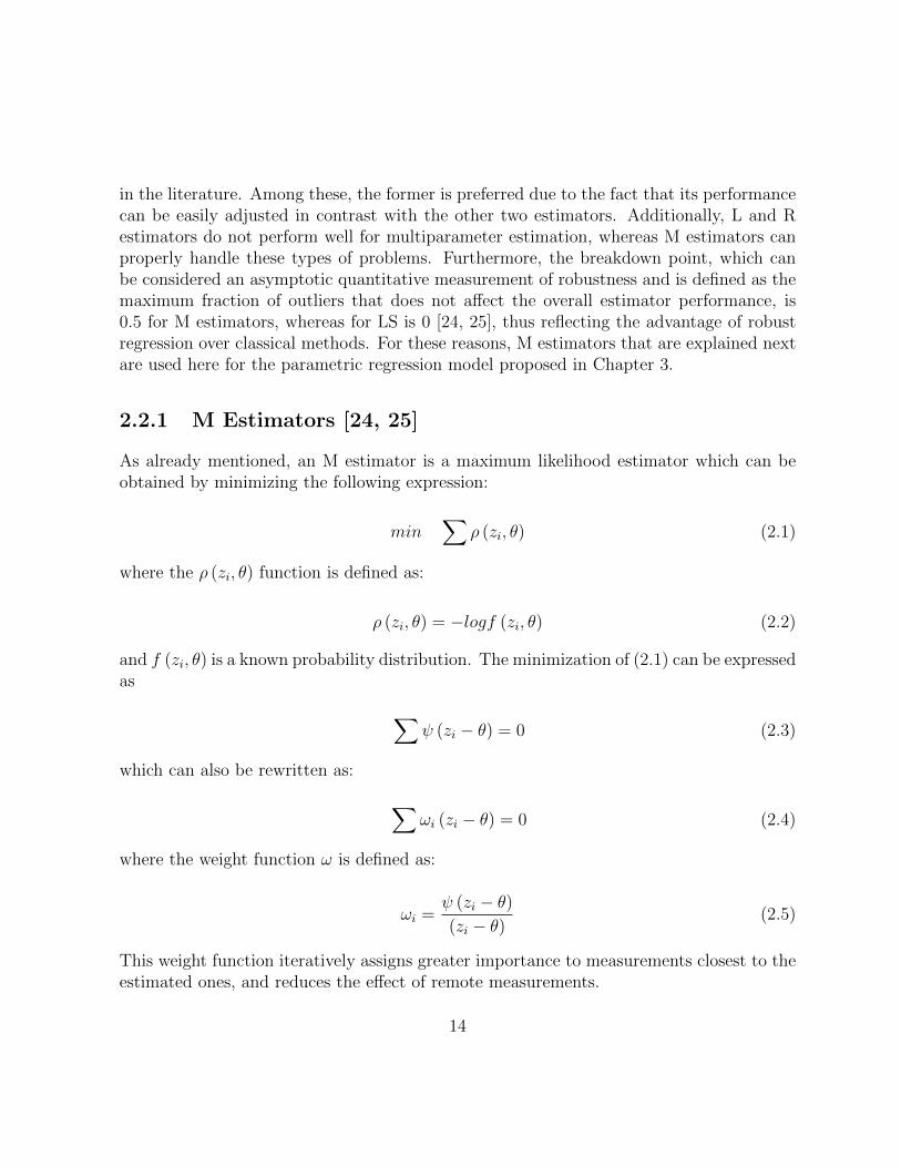
in the literature. Among these, the former is preferred due to the fact that its performancecan be easily adjusted in contrast with the other two estimators. Additionally, L and Restimators do not perform well for multiparameter estimation, whereas M estimators canproperly handle these types of problems. Furthermore, the breakdown point, which canbe considered an asymptotic quantitative measurement of robustness and is defined as themaximum fraction of outliers that does not affect the overall estimator performance, is0.5 for M estimators, whereas for LS is 0 [24, 25], thus reflecting the advantage of robustregression over classical methods. For these reasons, M estimators that are explained nextare used here for the parametric regression model proposed in Chapter 3.

2.2.1 M Estimators [24, 25]

As already mentioned, an M estimator is a maximum likelihood estimator which can beobtained by minimizing the following expression:

min∑

ρ (zi, θ) (2.1)

where the ρ (zi, θ) function is defined as:

ρ (zi, θ) = −logf (zi, θ) (2.2)

and f (zi, θ) is a known probability distribution. The minimization of (2.1) can be expressedas ∑

ψ (zi − θ) = 0 (2.3)

which can also be rewritten as: ∑ωi (zi − θ) = 0 (2.4)

where the weight function ω is defined as:

ωi =ψ (zi − θ)(zi − θ)

(2.5)

This weight function iteratively assigns greater importance to measurements closest to theestimated ones, and reduces the effect of remote measurements.

14

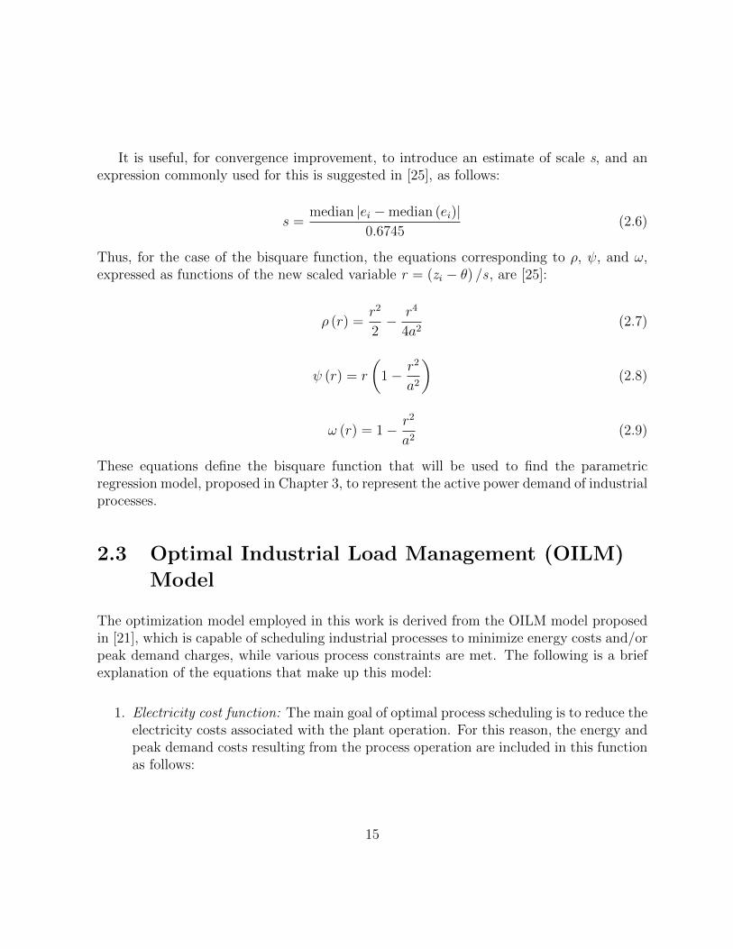
It is useful, for convergence improvement, to introduce an estimate of scale s, and anexpression commonly used for this is suggested in [25], as follows:

s =median |ei −median (ei)|

0.6745(2.6)

Thus, for the case of the bisquare function, the equations corresponding to ρ, ψ, and ω,expressed as functions of the new scaled variable r = (zi − θ) /s , are [25]:

ρ (r) =r2

2− r4

4a2(2.7)

ψ (r) = r

(1− r2

a2

)(2.8)

ω (r) = 1− r2

a2(2.9)

These equations define the bisquare function that will be used to find the parametricregression model, proposed in Chapter 3, to represent the active power demand of industrialprocesses.

2.3 Optimal Industrial Load Management (OILM)

Model

The optimization model employed in this work is derived from the OILM model proposedin [21], which is capable of scheduling industrial processes to minimize energy costs and/orpeak demand charges, while various process constraints are met. The following is a briefexplanation of the equations that make up this model:

1. Electricity cost function: The main goal of optimal process scheduling is to reduce theelectricity costs associated with the plant operation. For this reason, the energy andpeak demand costs resulting from the process operation are included in this functionas follows:

15

J =∑t

αtPtott + βPpeak (2.10)

2. Process coordination constraints: A process may or may not depend on the previousoperation of another process, so these constraints describe the possible interdepen-dency between processes. First, independent processes are scheduled within a timewindow, and minimum up-time and down-time requirements are considered. Sec-ond, different dependent processes are modeled. For instance, when the operationof one process depends on the previous operation of another, they are categorizedas sequential processes; on the other hand, if two or more processes are requiredtwo operate at the same time, they are considered parallel processes. The equationsthat maintain proper coordination of processes, which are relevant to this thesis, areinteger constraints as follows:

tonk,t+ toffk,t

≤ 1 (2.11)

tonk,t− toffk,t

= stk,t − stk,t−1 (2.12)

3. System constraints: In this work, system requirements are imposed using a supply-demand balance constraint. Thus, this equality equation, that also includes thestorage device operation, ensures that the demand is always met by the system, asfollows:

slnc,t−1 +∑m

orm,nc,t +∑q

irq,nc,t = slnc,t (2.13)

4. Power demand constraints: As already mentioned, the main objective of the opti-mal industrial operation is to minimize the electricity costs of an industrial facility.These constraints, therefore, take into account the individual as well as the totalpower demand required for the equipment and storage devices. Furthermore, peakdemand constraints are provided to control the maximum demand as required by thecustomer. These equations are as follows:

16

Pk,t = Fk (ork,t, irk,t) (2.14)

Pnc,t = Fnc (ornc,t, irnc,t) (2.15)

Ptott =∑k

Pk,t +∑nc

Pnc,t (2.16)

Ptott ≤ Ppeak (2.17)

Ppeak ≤ Pmax (2.18)

5. Operating constraints: The following inequality constraints keep all the process vari-ables within limits:

Rmin,k ≤ rk ≤ Rmax,k (2.19)

Slmin,nc≤ slnc ≤ Slmax,nc (2.20)

This OILM model provides a comprehensive framework for optimal industrial operation.Note that these equations are general, and hence they can be adapted for the actualoperating conditions of a given industrial facility. Therefore, this model is the foundationfor the model proposed in this work.

2.4 Optimization Methods and Solvers

An optimization problem basically focuses on finding the set of continuous and discretevariables that minimize or maximize an objective function satisfying a set of equality andinequality constraints. These problems, depending on the formulation of the objectivefunction, the constraint equations, and the type of decision variables, can be mainly cat-egorized into Linear Programming (LP), MILP, NLP, and MINLP problems. The latter,whose computational complexity is considered NP hard, is of great theoretical and practi-cal importance, since many real problems can be modeled as MINLP problems. A detaileddescription of the methods developed to deal with these problems, as well as related opti-mization solvers currently available are discussed next.

Formally, an MINLP problem can be represented by the following set of equations:

17

min g (x, y) (2.21)

subject to : d (x, y) ≤ 0 (2.22)

h (x, y) = 0 (2.23)

xεX, yεY

where g(x,y) is the objective function, d(x,y) is the set of linear and non-linear inequalityconstraints, h(x,y) is the set of linear and non-linear equality constraints, and X and Yare the set of continuous and discrete decision variables, respectively. Notice that MINLPproblems are composed of MILP and NLP subproblems, and global optimality cannot beguaranteed due to the integer constraints, even thought the nonlinear constraint could beconvex.

To solve the aforementioned optimization problem, many algorithms have been pro-posed in the literature. Broadly speaking, these methods can be classified in mathematicaland heuristic approaches. In general, the mathematical algorithms focus on solving relaxedNLP subproblems, which set lower bounds for the original MINLP problem, whereas fea-sible solutions to the MINLP problem set the upper limits. A comprehensive descriptionof these methods can be found in [26]. The state-of-the-art algorithms for solving thesetype of optimization problems are Branch and Bound (BB), Outer Approximations (OA),Generalized Bender Decomposition (GBD), and Extended Cutting Plane (ECP). On theother hand, heuristic search methods such as genetic algorithms, particle swarm optimiza-tion, ant colony, and simulated annealing have been used to solve MINLP problems.

Currently, there are a variety of commercial software packages to solve complex opti-mization problems. Among these, the General Algebraic Modeling System (GAMS) [27],used in this research, is very versatile for the mathematical modeling of large optimizationproblems. In addition, the model and the algorithm are independent of each other, therebyallowing flexibility for the use and evaluation of different solvers. Table 2.1 summarizesthe methods for each MINLP solver available in GAMS. The present work uses DICOPTto solve the optimization problem introduced in Chapter 4.

18

Table 2.1: GAMS solvers and algorithms for MINLP problems.

Solver Algorithm

AlphaECP ECPBARON BBCOINBONMIN BB,OA,ECPCOINCOUENNE BBDICOPT OAKNITRO BBLINDOGLOBAL BBSBB BB

2.5 Summary

The background required to develop an optimization model for industrial process schedul-ing was introduced in this chapter. DSM programs, especially DR programs oriented tomodify the load curve patterns such as valley filling, load clipping, and load shifting, werereviewed. Robust regression was briefly introduced as a method to reduce the outlier effectin a final regression model, and the bisquare method, an M estimator used to develop aparametric regression model in Chapter 3, was described in detailed. The general OILMmodel was briefly described as the basis for the optimization model proposed in Chapter 4.Finally, optimization problems mainly focused on MINLP problems and the mathematicalalgorithms commonly used to solve them were presented.

19

Chapter 3

Industrial Load Modeling

In this chapter, a polynomial regression model is introduced and developed for industrialloads. In particular, this parametric model is determined for the case of a chiller, whichis a thermodynamic equipment used to chill sensitive machinery in industrial processes.Hence, a chiller system is described in detail first, followed by its mathematical model forload management purposes.

3.1 Chiller Fundamentals

Before a feasible model can be proposed to estimate the active power consumption ofchillers, a detailed review of its basic operating principles as well as the main componentsof this equipment should be properly understood. Thus, this section discusses the basicoperating principles of a chiller system.

The refrigeration cycle, wherein a chemical substance called primary refrigerant canchange from liquid to gas and vice versa, by increasing or decreasing its internal energy orenthalpy, can be mainly carried out using vapor compression or absorption refrigerationcycles [28]. Nowadays, thermodynamic machinery employs the former to chill water asthe secondary coolant for water cooling systems. The first step of this cycle increases theenthalpy of the primary refrigerant without pressure and temperature variations; then,the pressure and temperature are increased by adding external energy to the refrigerant.Afterward, energy is released, thus decreasing the enthalpy, maintaining temperature andpressure constant, and at the same time, the temperature of the primary refrigerant isreduced. At the end, the pressure of the refrigerant decreases before a new refrigerationcycle begins again. This thermodynamic cycle is shown in Figure 3.1(b) [28].

20

6 HVAC Water Chillers and Cooling Towers

VAPOR COMPRESSION REFRIGERATION

RefRigeRation CyCle

The vapor compression cycle, wherein a chemical substance alternately changes from liquid to gas and from gas to liquid, actually consists of four distinct steps:

1. Compression. Lowpressure refrigerant gas is compressed, thus raising its pressure by expending mechanical energy. There is a corresponding increase in temperature along with the increased pressure.

2. Condensation. The highpressure, hightemperature gas is cooled by outdoor air or water that serves as a “heat sink” and condenses to a liquid form at high pressure.

3. Expansion. The highpressure liquid flows through an orifice in the expansion valve, thus reducing the pressure. A small portion of the liquid “flashes” to gas due to the pressure reduction.

4. Evaporation. The lowpressure liquid absorbs heat from indoor air or water and evaporates to a gas or vapor form. The lowpressure vapor flows to the compressor and the process repeats.

As shown in Figure 1.1, the vapor compression refrigeration system consists of four components that perform the four steps of the refrigeration cycle. The compressor raises the pressure of the initially lowpressure refrigerant gas. The

Evaporator Liquidgas

Liquid

gas

Highpressure

Low pressure

Expansionvalve

Compressor

Highpressure

Low pressure

Condenser

4

3

2 1

FIGURE 1.1 Basic components of the vapor compression refrigeration system. Condition point numbers correspond to points on pressure–enthalpy chart (Figure 1.3).

Dow

nloa

ded

by [

Uni

vers

ity o

f W

ater

loo]

at 1

1:57

22

Apr

il 20

15

(a) Water-cooled chiller.

h3,h4 h1 h2Enthalpy (Btu/lb)

P1

P2

Pres

sure

(ps

i)

1

23

4

(b) Refrigeration cycle.

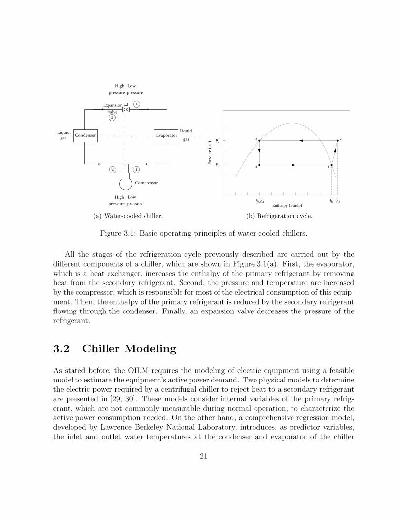
Figure 3.1: Basic operating principles of water-cooled chillers.

All the stages of the refrigeration cycle previously described are carried out by thedifferent components of a chiller, which are shown in Figure 3.1(a). First, the evaporator,which is a heat exchanger, increases the enthalpy of the primary refrigerant by removingheat from the secondary refrigerant. Second, the pressure and temperature are increasedby the compressor, which is responsible for most of the electrical consumption of this equip-ment. Then, the enthalpy of the primary refrigerant is reduced by the secondary refrigerantflowing through the condenser. Finally, an expansion valve decreases the pressure of therefrigerant.

3.2 Chiller Modeling

As stated before, the OILM requires the modeling of electric equipment using a feasiblemodel to estimate the equipment’s active power demand. Two physical models to determinethe electric power required by a centrifugal chiller to reject heat to a secondary refrigerantare presented in [29, 30]. These models consider internal variables of the primary refrig-erant, which are not commonly measurable during normal operation, to characterize theactive power consumption needed. On the other hand, a comprehensive regression model,developed by Lawrence Berkeley National Laboratory, introduces, as predictor variables,the inlet and outlet water temperatures at the condenser and evaporator of the chiller

21

Table 3.1: Variations of the general polynomial model.

Model p00 p01 p02 p03 p11 p22 p33 p12 p13 p23

1 X X X2 X X X X3 X X X X4 X X X X5 X X X X X X6 X X X X X X X X X

respectively [29]; the water flow rate, however, is considered constant in this model. Basedon these ideas, the following parametric polynomial regression model, as per [21], is pro-posed to account for chiller’s active power consumption in this research, considering thatthe water flow rates change:

Pch (Wf , Teo, Tci) = p00 + p01Wf + p02Teo + p03Tci + p11W2f + p22T

2eo

+ p33T2ci + p12WfTeo + p13WfTci + p23TeoTci + ε (3.1)

where ε is the error, and Wf , Teo, and Tci are the water flow rate and outlet water tem-perature at the evaporator, and inlet water temperature at the condenser, respectively.These variables, also known as predictor variables, determine the chiller’s active powerrequirement for normal operation.

3.2.1 Polynomial Model Fitting

In order to determine the most suitable regression model to estimate the power consump-tion of the aforementioned chillers, six variants of the general model (3.1), which are shownin Table 3.1, have been evaluated. The different options are ranked based on the results ob-tained for the square of the correlation coefficient (R2), Root Mean Square Error (RMSE),and energy error. The latter is defined as the prediction error of the regression model dueto the fitting process for a normal day of operation of the chillers.

Based on measurements of the relevant chiller model variables obtained from a measur-ing campaign at an automotive frame manufacturing facility in Ontario, between April 27and June 19, 2013, the bisquare approach explained in Section 2.2.1 is applied to estimate

22

Table 3.2: Polynomial fitting statistics.

Model 1 2 3 4 5 6

Chiller 1R2 [pu] 0.7688 0.8559 0.7696 0.7695 0.8596 0.8623

RMSE [kW] 18.64 9.49 18.67 18.65 9.50 10.13Energy Error[%] -4.78 -3.29 -4.96 -4.86 -3.62 -4.34

Chiller 2R2 [pu] 0.8686 0.9524 0.8688 0.8689 0.959 0.9618


Chiller 3R2 [pu] 0.7652 0.8809 0.7678 0.7677 0.8855 0.8865


Chiller 4R2 [pu] 0.8365 0.9645 0.8363 0.8365 0.9629 0.9691

RMSE [kW] 20.21 6.74 20.24 20.26 6.93 7.55Energy Error[%] 0.77 -1.39 0.80 0.77 -0.81 -2.45

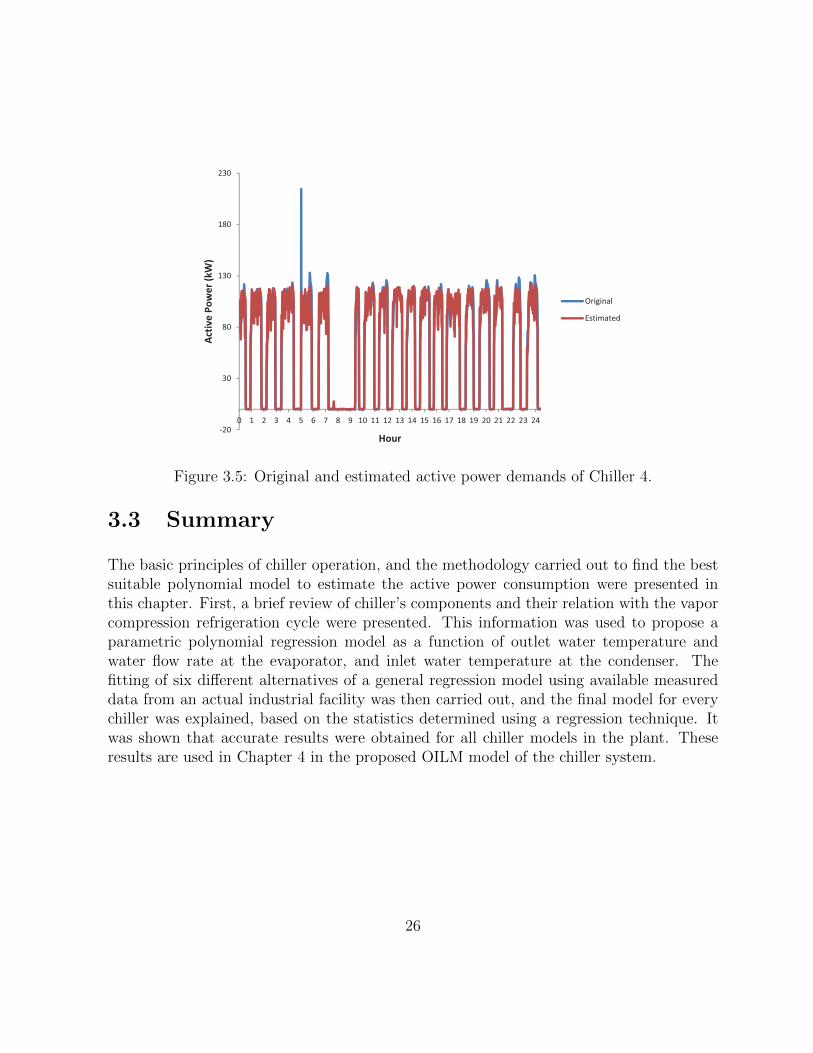
the coefficients of (3.1) for every chiller so that the influence of possible outliers in realdata for demand and process is reduced [25]. This results in the statistics and non-zerochiller polynomial model coefficients for the fitting process presented in Tables 3.2 and 3.3,respectively. Observe that the best results were obtained for Models 2, 5, and 6. Thesemodels include second degree terms of the water flow rate, which significantly influencesthe chiller power demand. Therefore, Model 5, based on the statistics in these tables, ischosen to estimate the power consumption of the chillers. Figures 3.2 to 3.5 show howeffectively the electric power estimated by the computed polynomials matches the actualconsumption for each chiller for a normal day of operation (June 7, 2013). Note also thatthe bisquare function reduces the effect of the outlier shown in Figure 3.5. This is possibledue to the fact that the regression method assigns a low weight to this measurement incomparison with the remaining data available for Chiller 4.

23

Table 3.3: Polynomial coefficients for Model 5.

Chiller 1 2 3 4

p01 [kW/GPM] 0.118937048 -0.378962631 -0.264400077 0.087629535p02 [kW/◦F] -0.644322437 -0.684596166 -0.264656196 -0.13625212p03 [kW/◦F] 0.428700392 0.463760361 0.177507725 0.09307501

p11 [kW/GPM2] -0.00074433 -0.000618612 -0.000680398 -0.000902843p12 [kW/(GPM)(◦F)] 0.006840054 0.019393174 0.012305408 0.005273654p13 [kW/(GPM)(◦F)] 0.001388705 -0.000704116 0.003165732 0.003987419

�20

0

20

40

60

80

100

120

140

0 1 2 3 4 5 6 7 8 9 10 11 12 13 14 15 16 17 18 19 20 21 22 23 24

Activ

e�Po

wer�(k

W)

Hour

Original

Estimated

�20

0

20

40

60

80

100

120

140

160

180

0 1 2 3 4 5 6 7 8 9 10 11 12 13 14 15 16 17 18 19 20 21 22 23 24

Activ

e�Po

wer�(k

W)

Hour

Original

Estimated

Figure 3.2: Original and estimated active power demands of Chiller 1.

24

�20

0

20

40

60

80

100

120

140

0 1 2 3 4 5 6 7 8 9 10 11 12 13 14 15 16 17 18 19 20 21 22 23 24

Activ

e�Po

wer�(k

W)

Hour

Original

Estimated

�20

0

20

40

60

80

100

120

140

160

180

0 1 2 3 4 5 6 7 8 9 10 11 12 13 14 15 16 17 18 19 20 21 22 23 24

Activ

e�Po

wer�(k

W)

Hour

Original

Estimated


�20

0

20

40

60

80

100

120

140

160

0 1 2 3 4 5 6 7 8 9 10 11 12 13 14 15 16 17 18 19 20 21 22 23 24

Activ

e�Po

wer�(k

W)

Hour

Original

Estimated

�20

30

80

130

180

230

0 1 2 3 4 5 6 7 8 9 10 11 12 13 14 15 16 17 18 19 20 21 22 23 24

Activ

e�Po

wer�(k

W)

Hour

Original

Estimated


25

�20

0

20

40

60

80

100

120

140

160

0 1 2 3 4 5 6 7 8 9 10 11 12 13 14 15 16 17 18 19 20 21 22 23 24

Activ

e�Po

wer�(k

W)

Hour

Original

Estimated

�20

30

80

130

180

230

0 1 2 3 4 5 6 7 8 9 10 11 12 13 14 15 16 17 18 19 20 21 22 23 24

Activ

e�Po

wer�(k

W)

Hour

Original

Estimated


3.3 Summary

The basic principles of chiller operation, and the methodology carried out to find the bestsuitable polynomial model to estimate the active power consumption were presented inthis chapter. First, a brief review of chiller’s components and their relation with the vaporcompression refrigeration cycle were presented. This information was used to propose aparametric polynomial regression model as a function of outlet water temperature andwater flow rate at the evaporator, and inlet water temperature at the condenser. Thefitting of six different alternatives of a general regression model using available measureddata from an actual industrial facility was then carried out, and the final model for everychiller was explained, based on the statistics determined using a regression technique. Itwas shown that accurate results were obtained for all chiller models in the plant. Theseresults are used in Chapter 4 in the proposed OILM model of the chiller system.

26

Chapter 4

Optimal Operation of an IndustrialProcess

The optimization model described in this chapter focuses on the minimization of energyand/or peak demand costs for the chiller system of an automotive frame manufacturingplant, based on the general OILM model described in Section 2.3. This model is usedto optimize the scheduling of 4 chillers in the plant water cooling system. The results ofapplying this model to the chiller system operation are compared with actual data andcosts obtained for the plant. Finally, improvements to the water cooling system based onthe proposed model are determined, so that higher electricity bill savings can be achieved.

4.1 Optimization Model for Chiller System Schedul-

ing

The goal of the optimal scheduling of industrial loads is to minimize the monthly electricitycosts, through increasing the efficiency of operation. Therefore, the following objectivefunction, which takes into account the energy and peak demand costs, charged to industrialcustomers by an LDC, is used here:

J = ∆T∑t

αtPTt + βPpeak (4.1)

where the parameters α, β, and ∆T can be adjusted depending on the main objectives ofthe plant operation.

27

Constraints associated with the operation of the chiller process starting with the activepower required by the process, estimated from the following equation, need also be con-sidered. This corresponds to the second-order polynomial model developed in Section 3.2,for the case of the chillers studied here:

Pchj,t= Fj

(Wfj,t , Teot , Tcit

)∀j, t (4.2)

The required chiller cooling capacity is obtained from:

Qej,t = Wfj,t (Teit − Teot)Kbt ∀j, t (4.3)

Additionally, considering the current operating practices, the Partial Load Ratio (PLR)and Coefficient of Performance (COP) of the chillers must be considered, as follows:

PLRj,t = Qej,t/Qerj ∀j, t (4.4)

COP j,t = Qej,t/(Pchj,t

Kpt

)∀j, t (4.5)

The water cooling system must be able to supply the requirements of the cooling load atevery time period. To ensure the system demand-supply balance, the following constraintsare needed:

Scapv,0 +∑j

Qej,tstj,t − scapv,t = Qlt ∀v, t = 1 (4.6)

scapv,t−1+∑j

Qej,tstj,t − scapv,t = Qlt ∀v, t ≥ 2 (4.7)

The initial storage capacity of the Chilled Water Storage (CWS) is considered in (4.6), and(4.7) to match the cooling supply, demand, and storage for the next time intervals. Hence,these two constraints ensure the system demand-supply balance at every instant of time.

To properly account the total amount of power required by the industrial processes,three additional constraints are needed. Thus, the following constraint determines the totalchiller active power in the water cooling system:

28

PTt =∑j

Pchj,tstj,t ∀t (4.8)

whereas the following constraints enforce the maximum active power limit imposed on theindustrial customer to reduce peak demand costs:

βPTt ≤ βPpeak ∀t (4.9)

βPpeak ≤ βPmax (4.10)

The coordination of chiller equipment in the industrial process is accomplished by:

tonj,t+ toffj,t

≤ 1 ∀j, t (4.11)

tonj,t− toffj,t

= stj,t − stj,t−1 ∀j, t (4.12)

where (4.11) prevents turn-on and turn-off decisions to be activated at the same timeinterval, and turn-on and turn-off decisions are coordinated through (4.12). Additionally,number of switching operations are limited by:

∑t

tonj,t≤ nsw ∀j (4.13)

Finally, all the variables used to characterize the chiller system have upper and lowerbounds. Hence, the feasible ranges for the chiller and storage tank variables are representedas follows:

Cmin,jstj,t ≤ cj,t ≤ Cmax,jstj,t ∀j, t (4.14)

Scapmin,v≤ scapv,t ≤ Scapmax,v

∀v, t (4.15)

The optimization model (4.1)-(4.15) considers active power requirements of the pro-cesses, supply-demand balance, interdependency between processes, and lower and upperlimits of the process variables. Depending on the cost reduction priority for the industrialfacility, the proposed optimization model permits the optimal chiller load scheduling by

29

minimizing the energy cost, peak demand charge, or both at the same time. For instance,choosing a zero value for the energy price parameter α would allow the minimization of thepeak demand charge only, whereas a zero value for peak demand charge β would optimallyschedule the chillers to reduce the associated energy costs. Thus, an industrial consumeris able to select an objective function that fits its specific concerns.

4.2 Study Case and Simulation Results

In this section, the aforementioned OILM model (4.1)-(4.15) is applied to the water coolingsystem of an automotive manufacturing company, which is described in some detail first.The goal is to determine the optimal scheduling of chillers, which are part of the watercooling system of the factory, in order to minimize the electricity costs for two differentcases:

• Case 1: Energy cost minimization.

• Case 2: Energy and peak-demand cost minimization.

4.2.1 Plant Description

One vital part of the normal operation of the automotive manufacturing company consid-ered is the cooling of certain processes and equipment. The industrial facility studied herehas a water cooling system whose schematic representation is shown in Figure 4.1, whichconsists of four chillers, a cooling tower, and a CWS. The water cooling process is carriedout by the chillers, whose detailed operation was described in Section 3.1. The main jobof these chillers is to chill the inner water flow (stored in the CWS) by removing the heattowards the outer water flow loop (through the cooling tower). The actual capacity ofheat disposal of this equipment depends on the inlet and outlet water temperature of thecondenser and evaporator, respectively. The total evaporator water flow output of thechillers is sent to the CWS, which helps to decouple instant demand requirements fromchiller operation, resulting in a more flexible chiller scheduling. Table 4.1 presents the maincharacteristic of the water cooling system. Additionally, a fixed temperature difference of7.5 ◦F between inlet and outlet water temperature at the evaporator is assumed.

30

CON

EVA

CHILLER 1

CON

EVA

CHILLER 2

CON

EVA

CHILLER 3

CON

EVA

CHILLER 4

From Process

To Process

Chilled Water Storage

Cooling Tower

Water Inlet

CON: Condenser

EVA: Evaporator

Figure 4.1: Water cooling system of the automotive manufacturing plant under study.

Table 4.1: Water cooling system equipment data.

Number of Chillers 4Compressor Power 180 HpCompressor Type CentrifugalChiller Capacity 156 tonsMinimum Water Flow Rate 50 GPMMaximum Water Flow Rate 500 GPMMaximum Chiller Switching Operations 200/month

Storage Capacity3456 gallons

35 tons

31

Table 4.2: Base and Case 1 comparison for May 2013.

Base Case Case 1 Savings [%]

Energy[$] 2,391.29 2,330.30 2.55

[kWh] 91650 94548 -3.16

Peak[$] 4,551.36 8,197.65 -80.11

[kW] 284 512 -80.11Total [$] 6,942.65 10,527.96 -51.64

The Independent Electric System Operator (IESO), which is responsible for clearingthe wholesale market in Ontario, splits the energy price in two components [31]: HourlyOntario Energy Price (HOEP) and Global Adjustment (GA), with the HOEP correspond-ing to an hourly energy price, and the GA corresponding to a variable monthly charge toaccount mainly for transmission congestion plus Feed-in Tariff (FIT) and DSM programs.In Ontario, an industrial customer with a peak demand greater than 5 MW is considereda Type A customer by an LDC, and GA is charged to power demand during peak hours.

For simulation purposes, the HOEP used here is based on the information published forMay 2013 in [31], which coincides with the measuring campaign dates, and it is assigned tothe parameter α for both cases. The GA value used, for this type of customer and basedon the information for July 2013 (the May 2013 bill was not available) provided by theindustrial customer, is 13.08 $/kW. In addition, Type A customers are also charged forpeak-demand, which was 2.93 $/kW for July 2013. A sample data set, for May 30, 2013,is provided in Table A.3 in Appendix A, for reference.

4.2.2 Case 1: Energy Cost Minimization

The optimization model described in Section 4.1, considering a zero value for the parameterβ, was used to obtain the optimal dispatch of the chillers for May 2013. Note that peak-demand minimization is not considered in this case. The results of this simulation areshown in Table 4.2. Observe that the energy cost is effectively reduced with respect tothe original energy cost; however, the peak-demand charge is almost twice the base cost.Hence, the final cost to operate the cooling system is more expensive than the current(base) operation.

Figure 4.2 shows the supply-demand balance in the water cooling system for May 30,2013. Notice the complementary operation of the storage tank to match the cooling demand

32

0 5 10 15 20 250

50

100

150

200

250

300

350

400

Hours

Co

olin

g L

oad

[to

ns]

Base−case total cooling demand (Ql)

Chiller cooling output (Qe)

Storage cooling output (scap)

Figure 4.2: Water cooling system load and storage capacity for May 30, 2013.

requirement, which is the same for all cases since this represents process output (demand),and to store the chiller’s cooling output when it exceeds the system cooling demand.

The total active power profile of the chillers is presented in Figure 4.3. Due to the factthat the present case does not minimize the peak-demand charge of the water cooling sys-tem, the optimization model tries to schedule the chillers considering the most economicaltime intervals only. Thus, for hours 4 and 6, when the HOEP is negative, the chiller activepower requirements are the highest of the day.

The PLR and COP of every chiller are shown in Figures 4.4 and 4.5 for May 30, 2013.Note that, for the negative energy prices at hours 4 and 6, the increasing active powerdemand reduces the COP, i.e., the compressor requires more power for the same coolingload supplied by the corresponding chiller.

33

512473

‐0.00309 ‐0.00182

‐0.01

‐0.005

0

0.005

0.01

0.015

0.02

0.025

0.03

0.035

0.04

0

100

200

300

400

500

600

0 5 10 15 20 25

HOEP

[$/kWh]

PT[kW]

Hours

230 230

‐0.00309

‐0.00182

‐0.01

‐0.005

0

0.005

0.01

0.015

0.02

0.025

0.03

0.035

0.04

0

50

100

150

200

250

0 5 10 15 20 25

HOEP

[$/kWh]

PT[kW]

Hours

Figure 4.3: Power demand profile of chillers and HOEP for May 30, 2013.

0 5 10 15 20 250

0.2

0.4

0.6

0.8

1

Hours

PL

R [

p.u

.]

Chiller 1

Chiller 2

Chiller 3

Chiller 4

Figure 4.4: PLR of chillers for May 30, 2013.

34

0 5 10 15 20 250

1

2

3

4

5

6

7

Hours

CO

P [

p.u

.]

Chiller 1

Chiller 2

Chiller 3

Chiller 4

Figure 4.5: COP of chillers for May 30, 2013.

Even though the optimal chiller scheduling successfully minimizes the energy costs, itdoes not accomplish the overall reduction of electricity costs. Hence, peak-demand costminimization needs to be included, as shown in the next section.

4.2.3 Case 2: Energy and Peak-Demand Cost Minimization

Energy and peak-demand costs are both minimized for May 2013 by the optimal chillerscheduling in this case. A value of 16.01 $/kW, which is equal to GA plus peak-demandconsumption charge, is considered for parameter β. Since the peak charges are higherthan the energy costs for this type of customer, by reducing peak demand during chilleroperation, final monthly savings should be attained. The final results for this case arepresented in Table 4.3. Observe that, even though the energy costs are higher than Case1, the total cost is less than that obtained for the base operation.

35

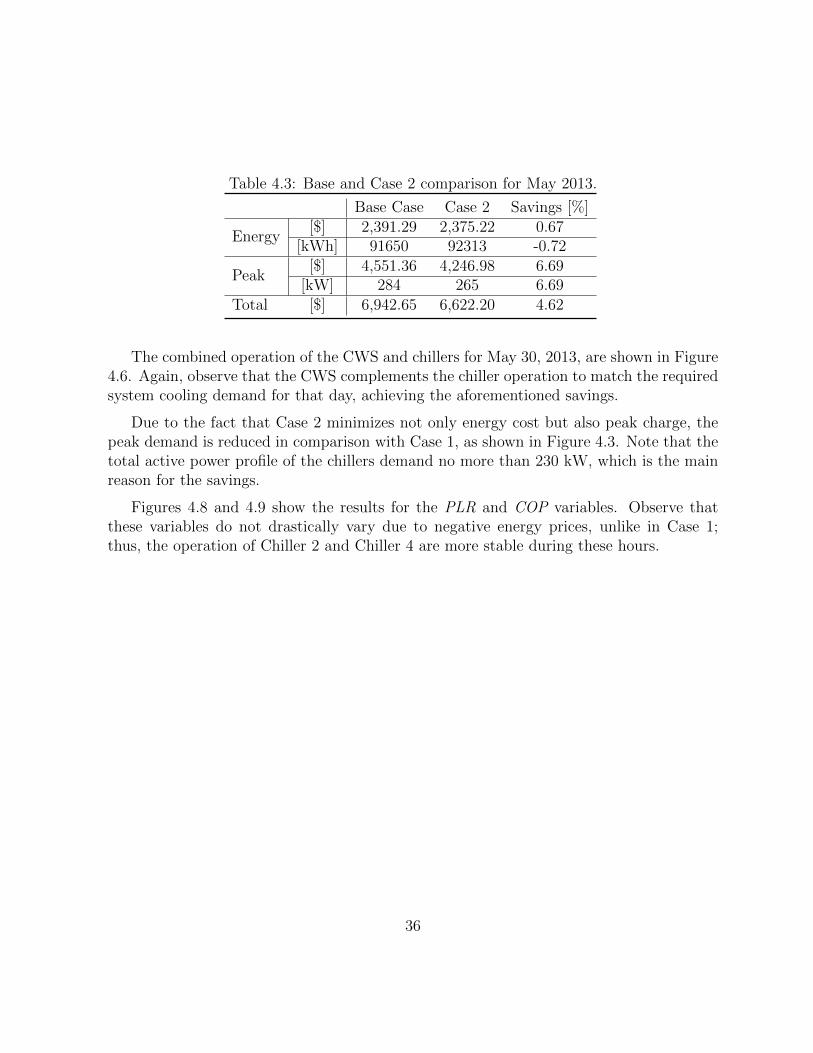
Table 4.3: Base and Case 2 comparison for May 2013.

Base Case Case 2 Savings [%]

Energy[$] 2,391.29 2,375.22 0.67

[kWh] 91650 92313 -0.72

Peak[$] 4,551.36 4,246.98 6.69

[kW] 284 265 6.69Total [$] 6,942.65 6,622.20 4.62

The combined operation of the CWS and chillers for May 30, 2013, are shown in Figure4.6. Again, observe that the CWS complements the chiller operation to match the requiredsystem cooling demand for that day, achieving the aforementioned savings.

Due to the fact that Case 2 minimizes not only energy cost but also peak charge, thepeak demand is reduced in comparison with Case 1, as shown in Figure 4.3. Note that thetotal active power profile of the chillers demand no more than 230 kW, which is the mainreason for the savings.

Figures 4.8 and 4.9 show the results for the PLR and COP variables. Observe thatthese variables do not drastically vary due to negative energy prices, unlike in Case 1;thus, the operation of Chiller 2 and Chiller 4 are more stable during these hours.

36

0 5 10 15 20 250

50

100

150

200

250

300

350

400

Hours

Co

olin

g L

oad

[to

ns]

Base−case total cooling demand (Ql)

Chiller cooling output (Qe)

Storage cooling output(scap)

Figure 4.6: Water cooling system load and storage capacity for May 30, 2013.

512473

‐0.00309 ‐0.00182

‐0.01

‐0.005

0

0.005

0.01

0.015

0.02

0.025

0.03

0.035

0.04

0

100

200

300

400

500

600

0 5 10 15 20 25

HOEP

[$/kWh]

PT[kW]

Hours

230 230

‐0.00309

‐0.00182

‐0.01

‐0.005

0

0.005

0.01

0.015

0.02

0.025

0.03

0.035

0.04

0

50

100

150

200

250

0 5 10 15 20 25

HOEP

[$/kWh]

PT[kW]

Hours

Figure 4.7: Power demand profile of chillers and HOEP for May 30, 2013.

37

0 5 10 15 20 250

0.2

0.4

0.6

0.8

1

Hours

PL

R [

p.u

.]

Chiller 1

Chiller 2

Chiller 3

Chiller 4

Figure 4.8: PLR of chillers for May 30, 2013.

0 5 10 15 20 250

1

2

3

4

5

6

7

Hours

CO

P [

p.u

.]

Chiller 1

Chiller 2

Chiller 3

Chiller 4

Figure 4.9: COP of chillers for May 30, 2013.

38

Table 4.4: Electricity cost savings for Case 1 and Case 2 for May 2013.

Cost Savings Case 1 (%) Case 2 (%)

Energy 2.55 0.67Peak -80.11 6.69Total -51.64 4.62

4.2.4 Comparison

Table 4.4 summarizes the final electricity cost savings obtained after the implementationof the optimization model for Cases 1 and 2. Notice that Case 2, where energy and peak-demand costs are minimized simultaneously, results in the best chiller operation. Case 1performs the savings better for energy cost reduction, but the total savings are negative,whereas total savings for Case 2 are almost 5% of the actual electricity costs. The latterare mainly due to the reduction of the total peak demand of the water cooling system.

The total peak demand profiles and energy consumption for May 2013, for the basecase and Cases 1 and 2, are shown in Figures 4.10 and 4.11, respectively. The four highestpeak demand days for Case 1 are a consequence of negative HOEP, which increases thefinal electricity bill. On the other hand, observe that the peak demand is maintained aslow as possible in Case 2, due to the minimization of peak-demand costs. In fact, the peakdemand profile for this case is less than the base peak demand of the water cooling systemfor most days. Additionally, energy consumption is slightly increased for both cases, withCase 2 having a smaller value than Case 1.

The chiller scheduling is performed considering the monthly maximum switching oper-ations allowed. This constraint is enforced by (4.13), and the final results are presented inFigure 4.12. Note that in both cases, the final switching operations are maintained belowthe limit set by the customer; in fact, the chiller operations are significantly reduced. Themain reason for this reduction is that Chillers 2 and 4 operate more frequently than Chillers1 and 3, as shown in Figure 4.13. In addition, the time interval ∆T of the optimizationmodel is 1 hour, and hence turn-on or turn-off decisions take place during that time period,thus limiting the number of possible switching operations.

39

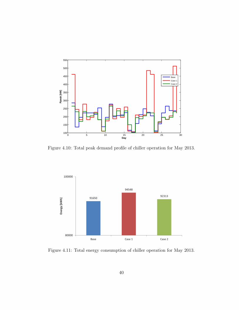
0 5 10 15 20 25 30100

150

200

250

300

350

400

450

500

550

Day

Pp

eak

[kW

]

Base

Case 1

Case 2

Figure 4.10: Total peak demand profile of chiller operation for May 2013.

329356 370

299

227

379

151

483

300

436

109

369

0

100

200

300

400

500

600

Chiller�1 Chiller�2 Chiller�3 Chiller�4

Hours�o

f�Ope

ratio

n

Base

Case�1

Case�2

91650

94548

92313

80000

100000

Base Case�1 Case�2

Energy�[k

Wh]

Figure 4.11: Total energy consumption of chiller operation for May 2013.

40

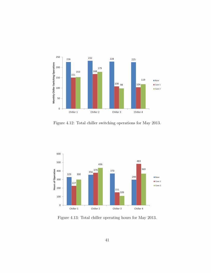
0

100

200

300

400

500

600

1 3 5 7 9 11 13 15 17 19 21 23 25 27 29

P pea

k[kW]

Day

Base

Case�1

Case�2

226 232 228 225

151168

108 104

153179

98

119

0

50

100

150

200

250


Mon

thly�Chiller�S

witching�Ope

ratio

ns

Base

Case�1

Case�2

Figure 4.12: Total chiller switching operations for May 2013.

329356 370

299

227

379

151

483

300

436

109

369

0

100

200

300

400

500

600


Hours�o

f�Ope

ratio

n

Base

Case�1

Case�2

91650

94548

92313

80000

100000

Base Case�1 Case�2

Energy�[k

Wh]

Figure 4.13: Total chiller operating hours for May 2013.

41

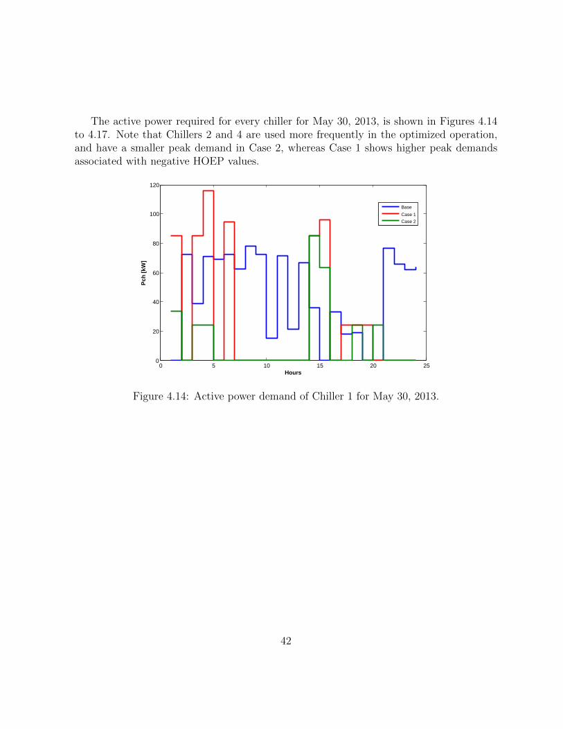
The active power required for every chiller for May 30, 2013, is shown in Figures 4.14to 4.17. Note that Chillers 2 and 4 are used more frequently in the optimized operation,and have a smaller peak demand in Case 2, whereas Case 1 shows higher peak demandsassociated with negative HOEP values.

0 5 10 15 20 250

20

40

60

80

100

120

Hours

Pch

[kW

]

Base

Case 1

Case 2

Figure 4.14: Active power demand of Chiller 1 for May 30, 2013.

42

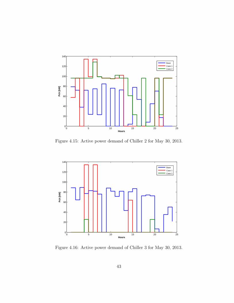
0 5 10 15 20 250

20

40

60

80

100

120

140

Hours

Pch

[kW

]

Base

Case 1

Case 2


0 5 10 15 20 250

20

40

60

80

100

120

140

Hours

Pch

[kW

]

Base

Case 1

Case 2


43

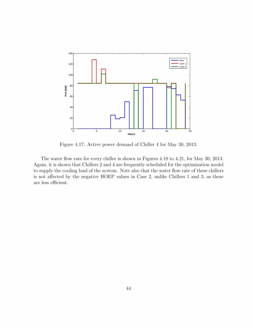
0 5 10 15 20 250

20

40

60

80

100

120

140

Hours

Pch

[kW

]

Base

Case 1

Case 2


The water flow rate for every chiller is shown in Figures 4.18 to 4.21, for May 30, 2013.Again, it is shown that Chillers 2 and 4 are frequently scheduled for the optimization modelto supply the cooling load of the system. Note also that the water flow rate of these chillersis not affected by the negative HOEP values in Case 2, unlike Chillers 1 and 3, as theseare less efficient.

44

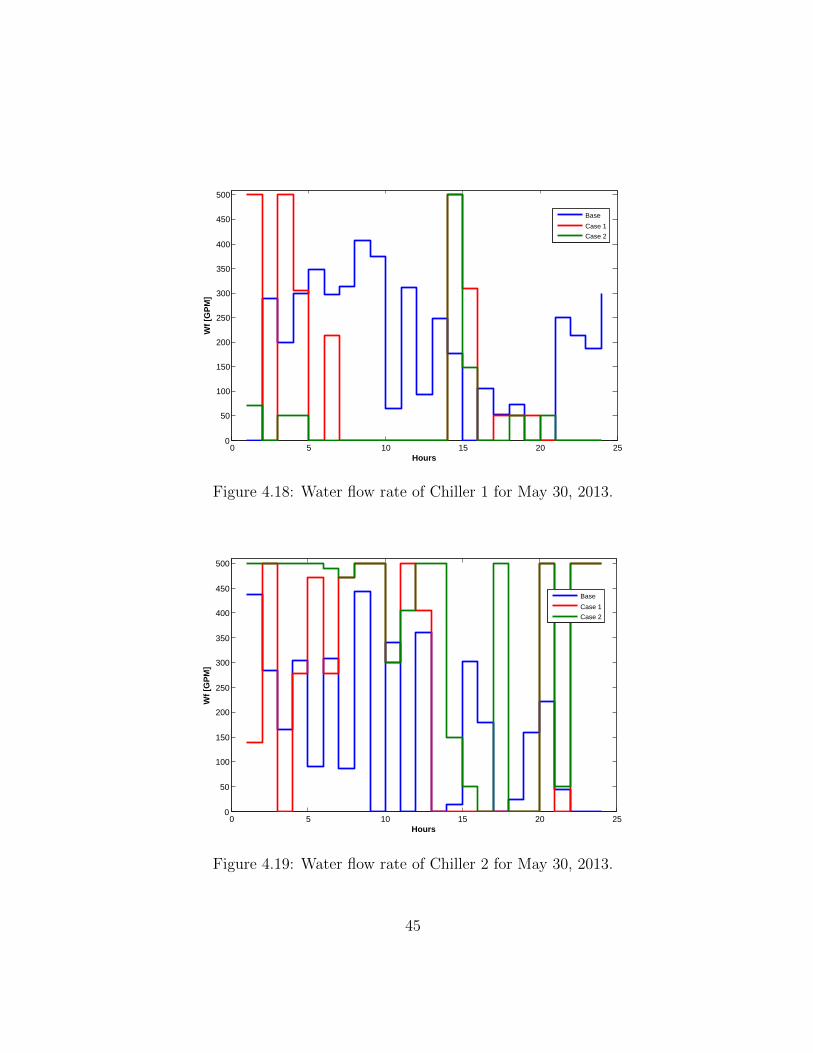
0 5 10 15 20 250

50

100

150

200

250

300

350

400

450

500

Hours

Wf

[GP

M]

Base

Case 1

Case 2

Figure 4.18: Water flow rate of Chiller 1 for May 30, 2013.

0 5 10 15 20 250

50

100

150

200

250

300

350

400

450

500

Hours

Wf

[GP

M]

Base

Case 1

Case 2


45

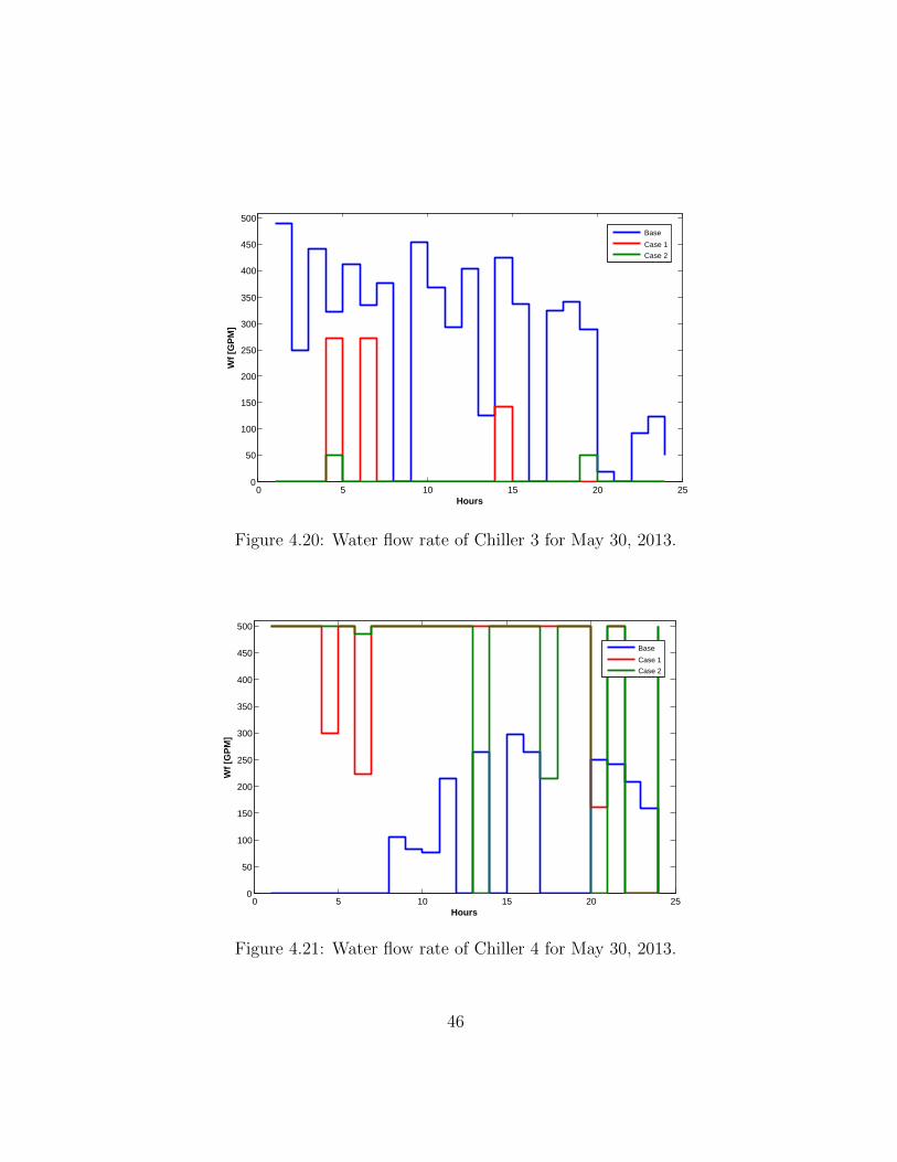
0 5 10 15 20 250

50

100

150

200

250

300

350

400

450

500

Hours

Wf

[GP

M]

Base

Case 1

Case 2


0 5 10 15 20 250

50

100

150

200

250

300

350

400

450

500

Hours

Wf

[GP

M]

Base

Case 1

Case 2


46

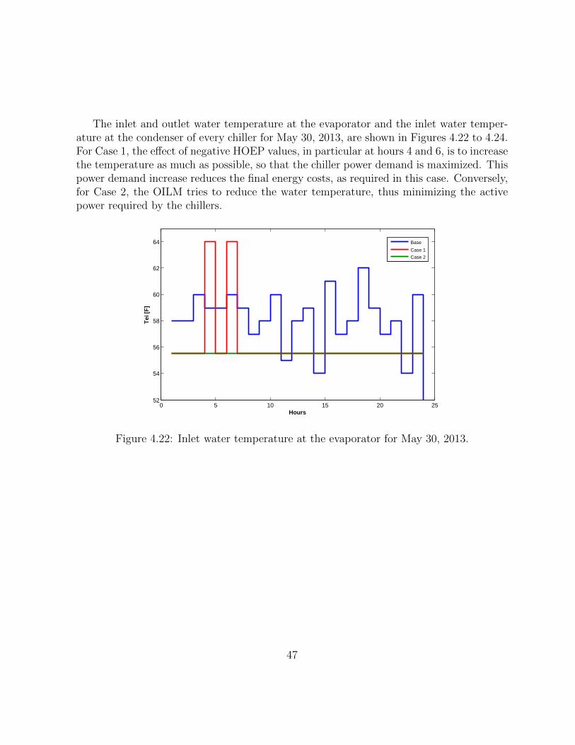
The inlet and outlet water temperature at the evaporator and the inlet water temper-ature at the condenser of every chiller for May 30, 2013, are shown in Figures 4.22 to 4.24.For Case 1, the effect of negative HOEP values, in particular at hours 4 and 6, is to increasethe temperature as much as possible, so that the chiller power demand is maximized. Thispower demand increase reduces the final energy costs, as required in this case. Conversely,for Case 2, the OILM tries to reduce the water temperature, thus minimizing the activepower required by the chillers.

0 5 10 15 20 2552

54

56

58

60

62

64

Hours

Tei

[F

]

Base

Case 1

Case 2

Figure 4.22: Inlet water temperature at the evaporator for May 30, 2013.

47

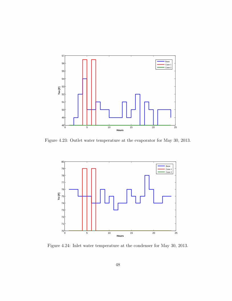
0 5 10 15 20 2548

49

50

51

52

53

54

55

56

57

Hours

Teo

[F

]

Base

Case 1

Case 2

Figure 4.23: Outlet water temperature at the evaporator for May 30, 2013.

0 5 10 15 20 2570

71

72

73

74

75

76

77

78

79

80

Hours

Tci

[F

]

Base

Case 1

Case 2

Figure 4.24: Inlet water temperature at the condenser for May 30, 2013.

48

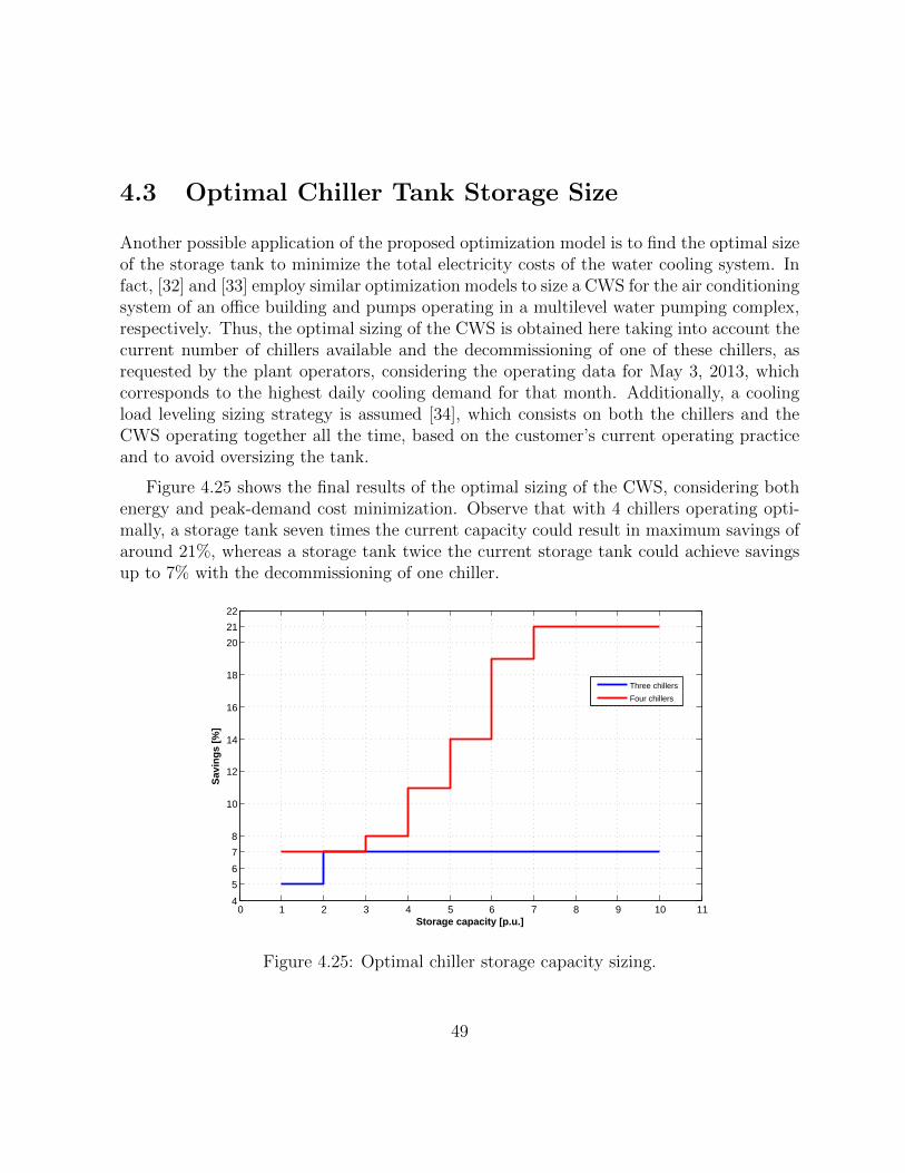
4.3 Optimal Chiller Tank Storage Size

Another possible application of the proposed optimization model is to find the optimal sizeof the storage tank to minimize the total electricity costs of the water cooling system. Infact, [32] and [33] employ similar optimization models to size a CWS for the air conditioningsystem of an office building and pumps operating in a multilevel water pumping complex,respectively. Thus, the optimal sizing of the CWS is obtained here taking into account thecurrent number of chillers available and the decommissioning of one of these chillers, asrequested by the plant operators, considering the operating data for May 3, 2013, whichcorresponds to the highest daily cooling demand for that month. Additionally, a coolingload leveling sizing strategy is assumed [34], which consists on both the chillers and theCWS operating together all the time, based on the customer’s current operating practiceand to avoid oversizing the tank.

Figure 4.25 shows the final results of the optimal sizing of the CWS, considering bothenergy and peak-demand cost minimization. Observe that with 4 chillers operating opti-mally, a storage tank seven times the current capacity could result in maximum savings ofaround 21%, whereas a storage tank twice the current storage tank could achieve savingsup to 7% with the decommissioning of one chiller.

0 1 2 3 4 5 6 7 8 9 10 114

5

6

7

8

10

12

14

16

18

20

21

22

Storage capacity [p.u.]

Sav

ing

s [%

]

Three chillers

Four chillers

Figure 4.25: Optimal chiller storage capacity sizing.

49

4.4 Summary

This chapter presented the application of the optimization model discussed in Chapter2 for the optimal scheduling of the chillers. A detailed description of the mathematicalmodel to minimize the electricity costs of a water cooling system in industrial facilitieswas provided. This model was then applied to schedule four chillers in a water coolingsystem of an automotive manufacturing company, and two cases were evaluated, namely,energy cost minimization, and energy and peak-demand cost minimization, resulting inthe latter yielding better electricity cost savings for the type of industrial facility studied.Indeed, savings of almost 7% were achieved for peak-demand cost minimization comparedto the base case. In all cases, the total monthly number of chiller switching operationswas maintained below the maximum allowed technically, with Chillers 2 and 4 operatingmore often than Chillers 1 and 3. These results demonstrate the significant advantages ofthe proposed optimization approach, which is shown to be feasible for supervisory controlapplications of real industrial processes.

Finally, the optimal size of an CWS, which is an essential component of a water coolingsystem, was determined considering all chillers and with a chiller out of service, with theformer requiring seven times the current storage capacity to maximize potential electricitysavings, whereas twice the current storage capacity is required to maximize possible sav-ings with reduced cooling capacity due to the decommissioning of one chiller. Thus, theoptimization model is shown to be not only capable of optimizing the current dispatch ofthe chillers, but also sizing the storage tank to maximize electricity cost savings.

50

Chapter 5

Conclusions

5.1 Summary and Conclusions

The present research focused on the optimal scheduling of industrial loads, based on theoptimization model proposed in [21], so that electricity costs are minimized. To evaluatethe effectiveness of this model, a chiller scheduling study was carried out in an automotivemanufacturing company.

The work and main findings, presented in this thesis, are the following:

• The necessity of improving the efficiency of current operating practices in industrialprocesses to improve the electrical network operation and thus reduce the correspond-ing environmental impacts, were presented in Chapter 1 as the main motivation forthe present work. Furthermore, a comprehensive literature review was also presented,covering general DSM programs and optimal approaches for process scheduling, anddiscussing the state of the art regarding process operation. Finally, the main objec-tives of the proposed research work were stated.

• DSM concepts and all the mathematical background required to develop optimizationmodels for industrial load scheduling were introduced in Chapter 2. DSM programs,general and industrial, were described and then, due to the fact that a parametricregression model was used for active power estimation of the chillers under study,robust estimation, mainly focused on M estimators, was described in detail. Sincethe optimization model used to schedule the chillers in this work is an application ofthe general OILM presented in [21], this model was then briefly discussed. Finally,

51

the main optimization concepts and solvers associated with MINLP problems werepresented.

• Chapter 3 discussed the modeling of chillers for optimal scheduling purposes, propos-ing a polynomial regression model. A detailed review of the vapor compressionrefrigeration cycle, which is the most commonly used, and how the chiller’s com-ponents are related to it was first presented. Based on chiller operation theory, asecond-degree polynomial model capable of estimating its active power demand wasdeveloped and validated, based on the bisquare method explained in Chapter 2 andmeasured chiller operation data at an automotive manufacturing plant; water flowrate and outlet temperature at the evaporator and inlet water temperature at thecondenser were considered as predictor variables for this model. Six different modelswere evaluated for every chiller to determine the best polynomial model, based onfitting process statistics, showing that it was accurate enough for scheduling purposesusing actual operation data.

• The optimal chiller scheduling for an automotive manufacturing plant was discussedin Chapter 4. Thus, the optimization model used for this task was first described indetail, with the main objective of minimizing electricity costs, which can basicallybe divided in energy and peak demand costs. Chiller and system constraints wereconsidered in the model, based on equipment limitation and customer preferences.Two cost minimization cases were then considered and contrasted with the currentchiller operation: energy cost minimization, and energy and peak-demand cost min-imization. The final results showed that even though the energy cost was reducedfor the first case, the total electricity cost was higher than the actual system oper-ation, due to increased peak demand associated with negative electrical energy costvalues. For the second case, conversely, the total cost was effectively reduced, withfinal savings of almost 5%, with respect to current operation. Peak-demand costs,were confirmed to be much more relevant for the industrial customer than energycosts; thus, peak-demand reduction should be the main goal for large industrial fa-cilities. Finally, the optimal size of the system storage tank was also determined forthe current number of chillers and with one chiller out of service, as requested bythe industrial customer. Using a scenario-based approach, the final results showedthat the water cooling system requires a storage tank seven times the actual capac-ity with the operation of four chillers to attain around 21% of maximum electricitycost savings, whereas the operation of a tank twice the actual capacity is enough toachieve total cost savings of up to 7% for the case of one chiller out of service. Theseresults demonstrate the advantages of the proposed optimization approach, which is

52

shown to be feasible for supervisory control applications of real industrial processes,and for optimal equipment sizing purposes.

5.2 Contributions

The contributions of the present research are the following:

• The OILM model proposed in [21] is applied to a water cooling system of an auto-motive frame manufacturing plant. The final results demonstrate and validate thefeasibility and benefits of the OILM approach.

• A novel second-order polynomial model, with water flow rate and outlet temperatureat the evaporator and inlet water temperature at the condenser as predictor variables,is developed and validated for estimation of chiller active power demand. This modelis shown to be suitable for optimal scheduling of chillers, and to accurately determinethe active power requirements for actual operating conditions, based on actual plantmeasurements.

• A new model for optimal scheduling of chillers for an industrial water cooling systemis proposed. The model is shown to minimize energy and peak-demand costs forchillers, considering relevant equipment and system constraints.

• The optimization model developed is tested for chiller scheduling to minimize energycost, and energy and peak-demand costs in an actual industrial facility. Electricitysavings are obtained for the latter, due to the type of industrial customer studied.

• The OILM is also applied to study enhancements to the water cooling system of theindustrial facility. Thus, it is shown that the size of the CWS can influence maximumelectricity savings due to optimal chiller scheduling.

The work presented here has been integrated into journal paper [35], and is expectedto be submitted after approval from the research partners.

5.3 Future Work

The following ideas would expand the optimal load management of industrial facilitiesshown in this thesis:

53

• The current OILM model is able to handle the optimization of continuous productionprocesses. Additional constraints should be included to consider batch productionrequirements.

• Industrial customers require the availability of on-site generation due to reliabilityconcerns, and the optimal operation of these generators could help to achieve furtherelectricity cost reductions. Thus, generation and electric storage constraints shouldbe integrated into the current OILM model.

• Due to the fact that optimal scheduling of chillers has been obtained using fixedvalues of parameters such as cooling demand and energy price, methods to reduce theinfluence of uncertainty on these parameter values should be considered. A controlmethod, such as MPC, could be applied to reduce the deviations of the forecastsagainst actual data.

54

APPENDICES

55

Appendix A

Water Cooling System SimulationData

Relevant data to perform the optimal chiller scheduling simulation is provided next. Noticethat the active power for every chiller, Pch, is estimated using the polynomial coefficientsgiven in Table 3.3.

Set : j = 4; t = 24; v = 1

Parameter : Kbt = Cpw(60)/12000

Table A.1: Parameter data.

Parameter Value

∆T 1 [hour]β 16.01 [$/kW]Cpw 8.33 [Btu/(USgal◦F)]Kpt 0.284 [tons/kW]nsw 7

56

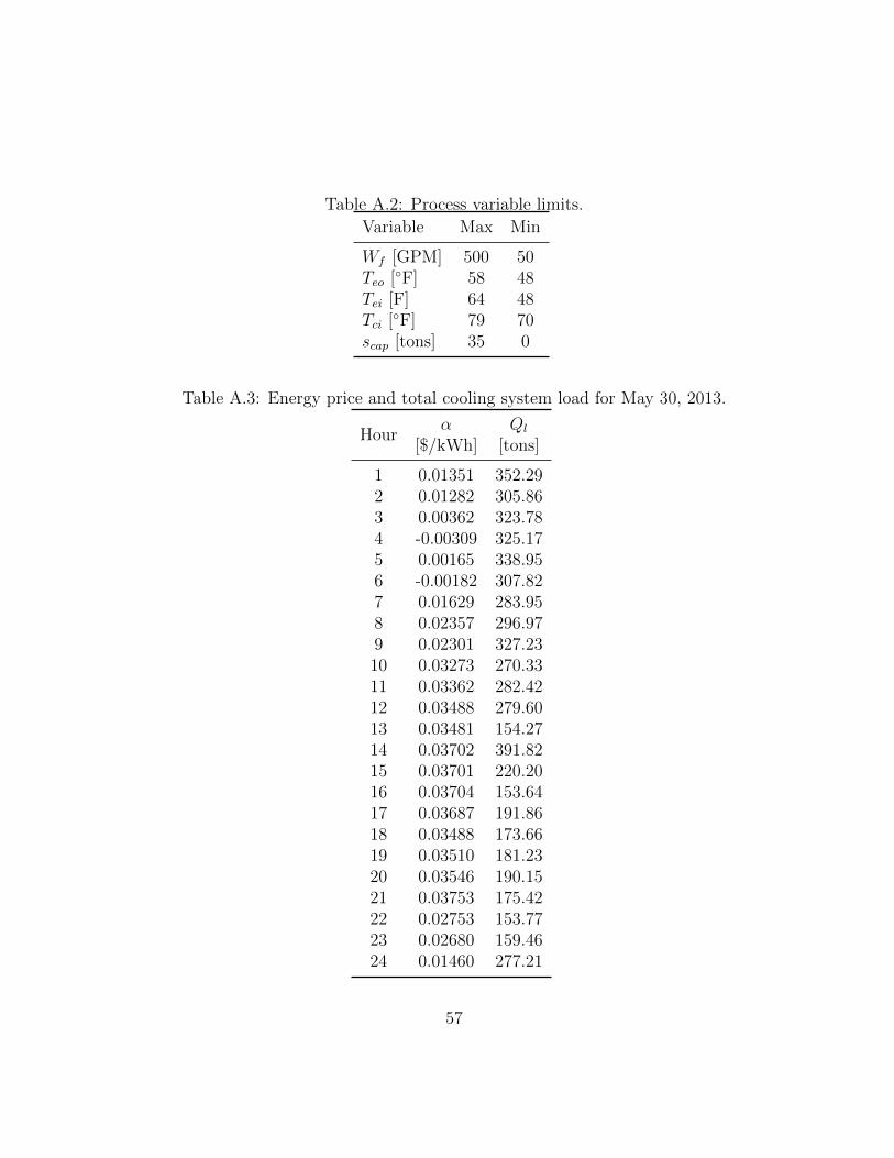
Table A.2: Process variable limits.

Variable Max Min

Wf [GPM] 500 50Teo [◦F] 58 48Tei [F] 64 48Tci [◦F] 79 70scap [tons] 35 0

Table A.3: Energy price and total cooling system load for May 30, 2013.

Hourα Ql

[$/kWh] [tons]

1 0.01351 352.292 0.01282 305.863 0.00362 323.784 -0.00309 325.175 0.00165 338.956 -0.00182 307.827 0.01629 283.958 0.02357 296.979 0.02301 327.2310 0.03273 270.3311 0.03362 282.4212 0.03488 279.6013 0.03481 154.2714 0.03702 391.8215 0.03701 220.2016 0.03704 153.6417 0.03687 191.8618 0.03488 173.6619 0.03510 181.2320 0.03546 190.1521 0.03753 175.4222 0.02753 153.7723 0.02680 159.4624 0.01460 277.21

57

References

[1] “Technology action plan: Industrial sector energy efficiency,” MajorEconomies Forum on Energy and Climate, December 2009. [Online].Available: http://www.majoreconomiesforum.org/images/stories/documents/MEF%20Industrial%20Sector%20EE%20TAP%2011Dec2009.pdf

[2] “Report on energy supply and demand in Canada - 2013 preliminary,” StatisticsCanada, February 2015. [Online]. Available: http://www.statcan.gc.ca/pub/57-003-x/57-003-x2015002-eng.pdf

[3] Independent Electric System Operator. [Online]. Available: https://saveonenergy.ca/

[4] “Electric load management in industry,” International Union for Electricity, January2009. [Online]. Available: http://www.uie.org/sites/default/files/generated/files/pages/LoadManagement.pdf

[5] W. Chen, X. Wang, J. Petersen, R. Tyagi, and J. Black, “Optimal scheduling ofdemand response events for electric utilities,” IEEE Transactions on Smart Grid,vol. 4, no. 4, pp. 2309–2319, 2013.

[6] S. Bu and F. R. Yu, “A game-theoretical scheme in the smart grid with demand-sidemanagement: Towards a smart cyber-physical power infrastructure,” IEEE Transac-tions on Emerging Topics in Computing, vol. 1, no. 1, pp. 22–32, 2013.

[7] H. M. Soliman and A. Leon-Garcia, “Game-theoretic demand-side management withstorage devices for the future smart grid,” IEEE Transactions on Smart Grid, vol. 5,no. 3, pp. 1475–1485, 2014.

[8] K. H. Nunna and S. Doolla, “Responsive end-user-based demand side management inmultimicrogrid environment,” IEEE Transactions on Industrial Informatics, vol. 10,no. 2, pp. 1262–1272, 2014.

58

http://www.majoreconomiesforum.org/images/stories/documents/MEF%20Industrial%20Sector%20EE%20TAP%2011Dec2009.pdf

http://www.majoreconomiesforum.org/images/stories/documents/MEF%20Industrial%20Sector%20EE%20TAP%2011Dec2009.pdf

http://www.statcan.gc.ca/pub/57-003-x/57-003-x2015002-eng.pdf

http://www.statcan.gc.ca/pub/57-003-x/57-003-x2015002-eng.pdf

https://saveonenergy.ca/

http://www.uie.org/sites/default/files/generated/files/pages/LoadManagement.pdf

http://www.uie.org/sites/default/files/generated/files/pages/LoadManagement.pdf

[9] A. Sheikhi, M. Rayati, S. Bahrami, and A. Mohammad Ranjbar, “Integrated demandside management game in smart energy hubs,” IEEE Transactions on Smart Grid,vol. 6, no. 2, pp. 675–683, 2015.

[10] S. Mohagheghi and N. Raji, “Dynamic demand response: A solution for improvedenergy efficiency for industrial customers,” IEEE Industry Applications Magazine,vol. 21, no. 2, pp. 54–62, 2015.

[11] S. Ashok, “Peak-load management in steel plants,” Applied Energy, vol. 83, no. 5, pp.413–424, 2006.

[12] H. Hadera, I. Harjunkoski, G. Sand, I. E. Grossmann, and S. Engell, “Optimization ofsteel production scheduling with complex time-sensitive electricity cost,” Computers& Chemical Engineering, vol. 76, pp. 117–136, 2015.

[13] W. Kong, T. Chai, J. Ding, and S. Yang, “Multifurnace optimization in electric smelt-ing plants by load scheduling and control,” IEEE Transactions on Automation Scienceand Engineering, vol. 11, no. 3, pp. 850–862, 2014.

[14] S. Ashok and R. Banerjee, “Optimal operation of industrial cogeneration for loadmanagement,” IEEE Transactions on Power Systems, vol. 18, no. 2, pp. 931–937,2003.

[15] Z. Wang, F. Gao, Q. Zhai, X. Guan, K. Liu, and D. Zhou, “An integrated optimiza-tion model for generation and batch production load scheduling in energy intensiveenterprise,” in Proc. Power and Energy Society General Meeting (PES). IEEE, 2012,pp. 1–8.

[16] S. Ashok and R. Banerjee, “An optimization mode for industrial load management,”IEEE Transactions on Power Systems, vol. 16, no. 4, pp. 879–884, 2001.

[17] C. Babu and S. Ashok, “Peak load management in electrolytic process industries,”IEEE Transactions on Power Systems, vol. 23, no. 2, pp. 399–405, 2008.

[18] A. Gholian, H. Mohsenian-Rad, Y. Hua, and J. Qin, “Optimal industrial load controlin smart grid: A case study for oil refineries,” in Proc. Power and Energy SocietyGeneral Meeting (PES). IEEE, 2013, pp. 1–5.

[19] A. Middelberg, J. Zhang, and X. Xia, “An optimal control model for load shifting–with application in the energy management of a colliery,” Applied Energy, vol. 86,no. 7, pp. 1266–1273, 2009.

59

[20] A. J. Van Staden, J. Zhang, and X. Xia, “A model predictive control strategy for loadshifting in a water pumping scheme with maximum demand charges,” Applied Energy,vol. 88, no. 12, pp. 4785–4794, 2011.

[21] S. Paudyal, C. Canizares, K. Bhattacharya et al., “Optimal operation of industrialenergy hubs in smart grids,” IEEE Transactions on Smart Grid, vol. 6, no. 2, pp.684–694, 2015.

[22] D. Y. Goswami and F. Kreith, Energy management and conservation handbook. CRCPress, 2007.

[23] “Estimating demand response market potential,” International Energy Agency,July 2005. [Online]. Available: http://www.ieadsm.org/Files/Tasks/Task%2013%20-%20Demand%20Response%20Resources/Market%20Potential%20Calculators%20Reports/Final%20Market%20Potential%20Summary%20Report FINAL.pdf

[24] P. J. Huber and E. M. Ronchetti, Robust statistics. Wiley, 2009.

[25] N. R. Draper, H. Smith, and E. Pownell, Applied regression analysis. Wiley NewYork, 1966, vol. 3.

[26] J. Lee and S. Leyffer, Mixed integer nonlinear programming. Springer Science &Business Media, 2011, vol. 154.

[27] R. E. Rosenthal, “GAMS–a user’s guide,” 2004.

[28] H. W. Stanford III, HVAC water chillers and cooling towers: fundamentals, applica-tion, and operation. CRC Press, 2011.

[29] P. Sreedharan, “Evaluation of chiller modeling approaches and their usability for faultdetection,” Lawrence Berkeley National Laboratory, 2001.

[30] J. Gordon, K. C. Ng, and H. T. Chua, “Centrifugal chillers: thermodynamic modellingand a diagnostic case study,” International Journal of Refrigeration, vol. 18, no. 4,pp. 253–257, 1995.

[31] “HOEP 2002-2014,” Independent Electric System Operator, January 2015. [Online].Available: http://www.ieso.ca/Pages/Power-Data/Data-Directory.aspx

[32] S. Ashok and R. Banerjee, “Optimal cool storage capacity for load management,”Energy, vol. 28, no. 2, pp. 115–126, 2003.

60

http://www.ieadsm.org/Files/Tasks/Task%2013%20-%20Demand%20Response%20Resources/Market%20Potential%20Calculators%20Reports/Final%20Market%20Potential%20Summary%20Report_FINAL.pdf



http://www.ieso.ca/Pages/Power-Data/Data-Directory.aspx

[33] H. Zhang, X. Xia, and J. Zhang, “Optimal sizing and operation of pumping systems toachieve energy efficiency and load shifting,” Electric Power Systems Research, vol. 86,pp. 41–50, 2012.

[34] 2007 ASHRAE Handbook - Heating, Ventilating, and Air-Conditioning Applications(I-P Edition). American Society of Heating, Refrigerating and Air-ConditioningEngineers, Inc., 2007.

[35] J. Munoz, F. Ordonez, V. Gutierrez, C. Canizares, K. Bhattacharya, and S. Paudyal,“Application of and optimal industrial load management model to industrial customersin the context of smart grids,” IEEE Transactions on Smart Grid, to be submitted.

[36] “Tracking industrial energy efficiency and CO2 emissions,” International En-ergy Agency, 2007. [Online]. Available: https://www.iea.org/publications/freepublications/publication/tracking emissions.pdf

61

https://www.iea.org/publications/freepublications/publication/tracking_emissions.pdf

https://www.iea.org/publications/freepublications/publication/tracking_emissions.pdf

optimal load management application for industrial consumers · je erson fabricio ord onez~ gir on...

Documents