optimal inventory control with retail pre-packs optimal inventory control with retail pre-packs 3...

Optimal Inventory Control with Retail Pre-PacksLong Gao

The A. Gary Anderson School of Management, University of California, Riverside, CA 92521, [email protected]

Douglas J. ThomasSmeal College of Business, The Pennsylvania State University, University Park, PA 16802, USA, [email protected]

Michael B. FreimerSignalDemand, San Francisco, CA 94111, USA, [email protected]

A pre-pack is a collection of items used in retail distribution. By grouping multiple units of one or more stock keeping

units (SKU), distribution and handling costs can be reduced; however, ordering flexibility at the retail outlet is limited.

This paper studies an inventory system at a retail level where both pre-packs and individual items (at additional handling

cost) can be ordered. For the single-SKU, single-period problem, we show that the optimal policy is to order into a

“band” with as few individual units as possible. For the multi-period problem with modular demand, the band policy is

still optimal, and the steady-state distribution of the target inventory position possesses a semi-uniform structure, which

greatly facilitates the computation of optimal policies and approximations under general demand. For the multi-SKU

case, the optimal policy has a generalized band structure. Our numerical results show that pre-pack use is beneficial when

facing stable and complementary demands, and substantial handling savings at the distribution center. The cost premium

of using simple policies, such as strict base-stock and batch-ordering (pre-packs only), can be substantial for medium

parameter ranges.

Key words: periodic review policies, pre-pack, batch ordering, steady-state distribution, demand correlation.

History: Current version: July 9, 2013

1. IntroductionIn production and distribution systems, materials often flow in fixed batch sizes or pre-packs, see, e.g.,

Litchfield and Narasimhan (2000), Smunt and Meredith (2000), and Blackburn and Scudder (2009). The

use of pre-packs has the advantage of smoothing production (Chao et al. 2005), increasing the productivity

in warehouses, reducing the number of order lines for retail stores, and improving the operating efficiency

of supply chains (van der Vlist 2007). On the other hand, goods that are produced and shipped in large

quantities or pre-packs are often disaggregated into individual items (called loose hereafter) at a break-bulk

point (i.e., a distribution center) before continuing on to the point of final consumption. While this break-

bulk operation incurs substantial facilities and handling costs, it might be worthwhile since it permits retail

locations to receive small, frequent replenishment.

This work was motivated by discussions with a U.S.-based apparel retailer with essentially two afore-

mentioned options for the distribution of goods. The first option is to have overseas contract manufacturers

produce, pack and ship a large quantity of a single SKU which is then unpacked at a domestic distribution

center. As stores place replenishment orders, individual items are selected and shipped from the distribution

center. Option two is to have overseas manufacturers package either multiple units of a single SKU or mul-

tiple units of similar SKUs (such as different sizes of the same style and color shirt) into smaller collections

1

Author: Optimal Inventory Control with Retail Pre-Packs 2

called pre-packs. These pre-packs are also received at the distribution center where they are subsequently

picked and shipped to retail stores. These options are illustrated in Figure 1.

Figure 1 Typical flow of goods for both pre-pack and non-pre-pack distribution.

The advantage of the pre-pack option in this case is that handling costs at the distribution center can be

substantially reduced, but ordering flexibility at the store is also limited. For the single-SKU setting, if there

is only one pre-pack configuration, and the store can only order pre-packs, the optimal inventory policy for

minimizing linear holding and shortage costs at the store is some version of the (R,nQ) policy—order an

integer number of pre-packs of size Q to bring the inventory above R once the inventory position is below

the reorder point R. In practice, the retail store may be able to order pre-packs as well as individual items,

and pre-packs may include multiple SKUs. For such settings, it is no longer clear what the optimal policy

will be.

This paper addresses the following inventory control questions in the presence of pre-pack and loose

ordering options: (1) What is the optimal policy if both pre-packs and loose can be ordered? (2) What are

the effects of the cost structure and the demand profile on the performance of the optimal policy? (3) What

is the cost of employing some commonly used simple policies? When are they good approximations to the

optimal policy?

To answer these questions, we consider a periodic-review inventory system with one distribution center

and one retail store. The random consumer demand occurs at the retail store only. Besides ordering an

integer number of pre-packs, the store can also order loose items at unit incremental handling penalty.

Unfulfilled demand is fully backlogged. The inventory policy seeks to minimize the sum of additional

handling cost of ordering loose units, inventory holding and backlogging costs.

Analytically, we characterize the structure of the optimal policy for a variety of scenarios, ranging from

traditional base-stock policy to the well-studied pre-pack-only (R,nQ) policy. In particular, we show that

for the single-SKU, single period case, the optimal policy under certain conditions possesses a simple band


structure where one orders the minimum number of loose items to get into this band. For the multi-period

case with Q-modular demand, the optimal policy still has the band structure due to the Q-periodicity of the

value function; additionally the target inventory position is semi-uniformly distributed in steady state. Based

on the band structure and the steady-state distribution of the inventory position, we develop an efficient

procedure to compute the optimal policy for modular demand as well as an effective approximation for

arbitrary discrete demand with sufficiently large volume. The band structure also extends to the multi-SKU

case, albeit in a more complicated form. Intuitively, when the additional cost of ordering individual units is

prohibitively large, the pre-pack-only policy is optimal for the single-SKU setting. Interestingly, this is not

the case for the multi-SKU setting for anything other than perfectly positively correlated demands due to

the inability of the pre-pack-only policy to adjust to the growing demand disparities between distinct SKUs

over time.

An important question related to the inventory control policy is the design of the pre-pack. In general,

accumulating more items into a pre-pack leads to greater handling savings but less ordering flexibility at

the retail outlet. In addition to this trade-off, firms must contend with different product mixes across retail

locations. For one particular product category, the apparel retailer mentioned above used two different kinds

of pre-packs: (1) a collection of different sizes of the same style-color combination and (2) a collection

of different colors of the same size-style (known as a “rainbow-pack.”) Consider the size-mix issue and

the data summarized in Table 1. This average size distribution shown in this table suggests that a pre-pack

consisting of of 1 small, 2 medium, 2 large and 1 extra large shirts might work reasonably well for most

stores, and in fact, this 1-2-2-1 size mix was precisely the pre-pack configuration in use. As suggested by

the min and max values in Table 1 though, such a pre-pack may work poorly for some stores. Some stores

sold no shirts in sizes small and medium while those sizes comprised 70% of sales at some other stores.

In addition to the product mix variation across stores, correlation in demand across items grouped together

will affect the utility of a particular pre-pack configuration. We first address the inventory control issues for

a given pre-pack configuration and then investigate the pre-pack design implications by varying pre-pack

size and demand correlation across SKUs.

Small Medium Large Extra LargeAvg 17% 29% 32% 22%Min 0% 0% 16% 0%Max 41% 54% 100% 40%

Table 1 Historical percentage of sales by size across over 400 apparel retail outlets in North America

2. Literature ReviewThis research is related to inventory control with batch ordering and inventory models with two batch sizes.

Batch-ordering policies have been well studied under various settings. For a single location, Morse (1958)

first studies a batch ordering (R,nQ) policy in a periodic review system. Veinott (1965) shows that the


(R,nQ) policy is optimal in both the finite and infinite period settings with zero setup cost, linear inven-

tory holding and shortage penalty costs. Zheng and Chen (1992) derive the long run average cost (holding

and backorder cost) associated with an (R,nQ) policy and develop an efficient heuristic algorithm to com-

pute the policy parameters with lower and upper bounds. Chen (2000) generalized Veinott’s optimality

result to multi-echelon settings where each stage is restricted to a batch-ordering policy. Chao and Zhou

(2009) further extend Chen’s work to the multi-echelon setting with both batch ordering and fixed replen-

ishment intervals. Cachon (2001) provides exact valuation methods for the periodic review systems with

one warehouse and multiple identical retailers under a batch-ordering policy. Axsater (2000) gives exact

results for continuous review systems with compound Poisson demand and nonidentical retailers. Ander-

sson et al. (1998) investigate the (R,nQ) policies in coordinating a decentralized inventory system where

the stochastic lead times perceived by the retailers are replaced by their correct averages. Based on a simple

approximation, they develop near-optimal reorder points and bounds for the approximation errors. Berling

and Marklund (2006) examine the performance of continuous review (R,Q) policies in a one-warehouse

multiple-retailer context, and offer a practical means to achieve coordinated control of large size systems. In

contrast to the aforementioned work with only batch ordering options, our paper deals with situations with

both pre-pack and loose ordering options. Moreover, we establish the suboptimality of the (R,nQ) policy

in the general multi-SKU case.

A key notion in analyzing many batch-ordering systems is the uniformity property—the steady state

distribution of the inventory position after ordering is uniformly distributed. This property was first shown

by Hadley and Whitin (1961) under the assumption of Poisson demands and constant or gamma lead time.

Song (2000) extends this uniform equilibrium distribution result to the multiple item setting. Chen (1998)

extended the uniformity property to a continuous review, two-echelon inventory system with interdependent

demands. We contribute to the literature by establishing a semi-uniform property for the system with both

ordering options and modular demand.

The research closest to our study is Henig et al. (1997), and Parkinson and McCormick (2005). Henig

et al. (1997) analyze a joint inventory control and contract design problem in which a fixed quantity R is

available at no incremental cost and at a given frequency. Quantities greater than R may be ordered with a

per-unit penalty. As with the problem addressed in this paper, the base stock policy is not optimal; instead

the policy has two critical levels which determine whether an amount greater than R should be acquired.

Parkinson and McCormick (2005) also consider a problem similar to the one discussed in this paper, moti-

vated by a chemical supplier with large and small ocean tankers. In this problem a single product is available

via two delivery sizes (pre-packs), one of which is twice as large as the other (our model does not have this

restriction). However, neither of them considers multi-SKU pre-packs (and consequently the impact of the

demand correlation) and steady-state distribution of the inventory position. Chen et al. (2012) address the

problem of designing and ordering pre-packs for pre-season planning. The authors develop an optimiza-

tion model and heuristic solution approach for pre-season planning and ordering assuming deterministic

demand. Our work is complementary to theirs in the sense that we focus on the ongoing management of the

inventory system under stochastic demand.


3. Single SKU Pre-packThe primary benefit of using a pre-pack is a reduction in handling costs through the distribution network.

We model this handling efficiency by specifying an incremental per-unit cost penalty δ for units ordered

loose. We assume δ > 0 unless specified otherwise. Table 2 summarizes the main notation.

Table 2 Notationξ random demand; ξ ∼ f ; Eξ = µ, varξ = σ2

b unit backorder cost (adjusted)h unit holding cost (adjusted)δ unit penalty for ordering loose itemsβ discount factor; β ∈ (0,1)

q loose order quantity for the 1-SKU case; q∈Rk for the k-SKU caseQ pre-pack size; Q∈Rk

+ for the k-SKU casex initial inventory with recurrent state space X for the 1-SKU case; x∈Rk for the k-SKU casey post pre-pack position; y= x+nQ; y for the k-SKU caseI target position; I = y+ q; I for the k-SKU caseR indifferent level; R for the k-SKU caseS base stock level; S for the k-SKU caseZ loose stock level; Z for the k-SKU case

y(x) pre-pack function; the highest inventory position below R+Q achievable by ordering pre-packs1A indicator function of event A

We consider a periodic-review, single-product inventory system with both pre-pack and loose ordering

options to fulfill stationary random demand ξ ∼ f . The unit variable costs for ordering pre-packs and loose

items are c0 and c1; hence the unit penalty cost δ = c1 − c0. The sequence of events in each period unfolds

as follows: First, we observe the initial inventory x ∈ X . Then an order is placed for n ∈ Z+ pre-packs of

size Q ∈ R+ and q ∈ R+ units of loose to reach the target inventory position I = x+ q + nQ. The order

arrives, and random demand ξ is realized and satisfied to the extent possible. Unfulfilled demand is fully

backlogged at unit shortage cost b. The leftover inventory incurs unit holding cost h. The objective is to

minimize the expected total discounted cost V (x) for an infinite horizon. The problem can be formulated

as a Markov decision process with the following Bellman equation:

V (x) = miny=x+nQ:n∈Z+

minI≥x+nQ

{ c0(y−x)+ c1(I − y)+ hE(I − ξ)+ + bE(ξ− I)+ +βEV (I − ξ)} .

This formulation can be simplified by applying the transformation V (x) = V (x) + c0x − (1 − β)−1c0µ

(Song and Zipkin 1993), and the identities I =E(I − ξ)+µ=E(I − ξ)+ −E(ξ− I)+ +µ:

V (x) = minn∈Z+

minI≥x+nQ

{ δ(I −x−nQ)+hE(I − ξ)+ + bE(ξ− I)+ +βEV (I − ξ)} , (1)

with the adjusted costs δ= c1 − c0, h= h− (1−β)c0, and b= b+(1−β)c0.

In the reminder of the section, we first characterize the structure of the optimal policy for the single-

period model in §3.1, then extend it to the multi-period setting and derive the steady state distribution for

the target inventory position in §3.2.


3.1. Single Period Analysis

Because the ordering sequence is inconsequential, we can solve problem (1) in two steps: First, solve the

pre-pack problem for ordering n pre-packs to the pre-pack position y = x+ nQ; second, solve the loose

problem for ordering q loose units to the loose position I = y + q. Hence the optimal policy (y∗, I∗) pre-

scribes the two positions for each initial inventory x by solving the following program:

V (x) =miny

{H(y) : y= x+nQ,n∈Z+

}, pre-pack problem (2)

H(y) =minI

{ δ(I − y)+G(I) : I ≥ y } , loose problem (3)

G(I) = hE(I − ξ)+ + bE(ξ− I)+, (4)

where G(y) is the inventory cost, including the holding and shortage costs. It is easily verified that G(I) is

convex and coercive. H(y) is also convex and coercive for δ > 0 (by the convexity of G, and parts (b), (c),

and (d) of the convexity Lemma 1 in Appendix).1 See Figure 2 for a depiction of these properties.

To characterize the optimal policy, we define three anchoring points and a function: (1) pre-pack target

S, (2) loose target Z, (3) indifference target R, and (4) the pre-pack function y(x).

First, define the pre-pack target S ≡ argminI G(I), i.e.,

G′(S) = 0. (5)

Lemma 2.(a) below establishes that S = argminy H(y). Thus, S is the unconstrained optimal inventory

position for ordering pre-packs.

Second, define the loose target Z ≡ argminI [δ(I − y)+G(I)], i.e.,

Z =

{−∞, if δ+G′(I)> 0,∀I ∈R,[G′]−1(−δ), otherwise.

(6)

where [G′]−1 is the inverse function of the derivative of G. The convexity of G ensures that Z is well-

defined. Intuitively, Z is the unconstrained optimizer for the loose decision I .

Third, define the indifference target R by

H(R) =H(R+Q). (7)

The convexity and coerciveness of H ensure that R is well-defined and that R ≤ S ≤ R+Q. Intuitively,

R is the inventory position where the cost of ordering loose items up to Z (if feasible) is the same as the

cost of ordering one more pre-pack to R+Q. Hence R facilitates the comparison of the pre-pack decisions

y= x+nQ,n∈Z+.

Fourth, define the pre-pack function y(x) by

y(x)≡max{x+nQ : x+nQ≤R+Q,n∈Z+ } . (8)

1 A function f :R→R is coercive if lim∥x∥→∞ f(x) =∞.


By construction, y(x) is Q-periodic for x≤R+Q, i.e.,

y(x) = y(x−Q), ∀x≤R+Q. (9)

Thus y(x) is the highest position less than or equal to R+Q achieved by ordering only pre-packs given

initial inventory x≤R+Q. The purpose of y(x) is to partition the state space X for characterization.

The anchoring points S, Z and R have the following properties. See Figure 2 for an illustration.

LEMMA 2. (a) The pre-pack target S = argminy H(y), i.e., H ′(S) = 0.

(b) R≤ S ≤R+Q and Z ≤ S.

0 Inventory Position

Cost

Funct

ions

1

1

1

2

2

3

R+Q

δ(I − y) + G(I)

SR Z

(y(x),Z)

3

(y(x), y(x))

G(I)

Figure 2 Single-SKU Optimal Policy

The following theorem characterizes the optimal policy for the single-period, single-SKU problem.

THEOREM 1. Consider the single-period, single-SKU problem in (2).

(a) If Z ≤R, the (R,nQ) policy is optimal; i.e., order pre-packs only into the band (R,R+Q]. Formally,

(y∗, I∗) = (y(x), y(x)). (10)

(b) If Z > R, the band [Z,R+Q] policy is optimal. Specifically, if y(x) ∈ (R,Z], order pre-packs up to

y(x) and then order Z − y(x) loose units; if y(x) ∈ (Z,R+Q], order up to y(x) using pre-packs only.

Formally,

(y∗, I∗) =

{(y(x),Z), if y(x)∈ (R,Z],

(y(x), y(x)), if y(x)∈ (Z,R+Q].(11)

(c) if the penalty cost δ= 0, then the base-stock S policy is optimal.


Theorem 1 provides a unified framework for characterizing the whole spectrum of inventory polices.

Parts (a) and (c) establish, for the two extremes, the optimality of two well-known policies— the (R,nQ)

and base-stock policies. Part (b) demonstrates that under certain conditions the optimal policy exhibits a

band structure; see Figure 2 for an illustration. In the inventory literature, the band structure also arises

in the (s,S) policy (Clark and Scarf 1960). However, the underlying mechanisms for order batching are

different. In the (s,S) policy it is driven by the fixed ordering cost; in the [Z,R+Q] policy it arises from

the cheaper pre-pack ordering option.

THEOREM 2. The optimal value function V (x) for the problem (2) is Q-periodic for x≤R+Q.

Theorem 2 reveals that, unlike a conventional convex ordering cost, the cost structure in the presence of

both pre-pack and loose ordering options induces periodic behavior in both the optimal policy and the value

function. This behavior substantially complicates the multi-period problem. Fig. 3 illustrates the impact of

the periodic behavior on V (x). As a result, the conventional backward induction approach for establishing

structural results breaks down. Without additional assumptions, the exact characterization for the multi-

period case appears unattainable.

0 10 20 30 40 5052

54

56

58

60

62

64

66

68

70

Inventory:I

Cos

t

E[V (I − ξ)]

V (x)

G(I)

Figure 3 Non-convexity of value function V (x) and E[V (I − ξ)]: ξ ∼N (30,52), Q= 17, δ= 0.4, h= 1, b= 1

3.2. Multi-Period Analysis

The single-period model in §3.1 extends to the infinite horizon if we redefine G(I) as

G(I)≡ hE(I − ξ)+ + bE(ξ− I)+ +βEV (I − ξ). (12)

To extend the structural results in §3.1 by backward induction, we need to first establish the convexity

of G(I), which in turn requires the convexity of V (x). Theorem 2, however, demonstrates that the Q-

periodicity of V (x) destroys its convexity even in the single-period case. Although the optimal policy can


be obtained by solving (1) with standard value- or policy-iteration algorithms, without the guidance of the

policy structure, we have to exhaustively search the space Z+×R for the optimal decision (n(x), I(x)) for

each x. The computation becomes even more expensive for multi-SKU cases.

In the rest of this section, we focus on demand with the modulus property where sharp characterization

is possible.2 Let ξQ be the residue (remainder) of mod(ξ,Q), i.e., ξ = ξQ + nQ, for some n ∈ Z+ and

0≤ ξQ <Q.

ASSUMPTION 1. The random demand ξ is Q-modular; i.e., ξQ ∼U [0,Q− 1].

That is, the residue (mod Q) of demand is uniformly distributed. In essence, it requires the demand distri-

bution f satisfies ∑n∈Z+

f(i+nQ) =1

Q, ∀ i= 0, . . . ,Q− 1. (13)

For example, any uniform distributions U [m,m+nQ− 1]m,n∈Z+, and triangular distributions

f(x) =

{x

(nQ)2, x∈ [0, nQ],

− x(nQ)2

+ 2nQ

, x∈ [nQ,2nQ],

are Q-modular. The following lemma is critical for characterization.

LEMMA 3. If the random variable ξ is Q-modular, and the function V (I) is Q-periodic for I ≤R+Q,

then EV (I − ξ) is a constant for I ≤R+Q.

We now characterize the optimal policy in the multi-period setting.

THEOREM 3 (Optimal Policy). Consider the infinite horizon, single-SKU problem in (1) with Q-

modular demand.

(a) If Z ≤R, the (R,nQ) policy is optimal.

(b) If Z >R, the band policy [Z,B+Q] is optimal.

(c) If the penalty cost δ= 0, the base-stock policy with order-up-to level S is optimal.

(d) The optimal value function V (I) is Q-periodic for x≤B+Q.

For a given policy, the ending inventory I forms a Markov process. We now consider the stationary

distribution ϕ of I . For the (R,nQ) policy, Hadley and Whitin (1961) proved the uniformity property of ϕ.

THEOREM 4 (Hadley and Whitin, 1961). Consider a periodic review, stationary, infinite horizon

(R,nQ) inventory system with random demand ξ. If the Markov chain is irreducible, then the steady-state

inventory position is uniformly distributed over the set {R+1,R+2, . . . ,R+Q }.

The uniformity property is the central notion in the batch ordering literature. It holds for an arbitrary demand

distribution. In the context of multiple pre-packs, we have shown that under Z ≤ R the optimal policy is

also an (R,nQ) policy, and therefore the Hadley and Whitin theorem applies. Unfortunately there is no

such general result when Z >R. We can, however, establish a similar theorem for Q-modular demand.

2 We thank one of the anonymous referees for this key insight.


THEOREM 5 (Semi-uniform distribution). Under the condition Z >R, if demand ξ is Q-modular, and

the band policy [Z,B+Q] is implemented, then the ending inventory has a semi-uniform distribution:

ϕ=

(Z −B

Q,1

Q, . . . ,

1

Q

). (14)

Theorem 5 makes two theoretical contributions. The first is the simplicity of the distribution form. As

such, it generalizes the uniformity property from the pre-pack-only case to the setting where both pre-pack

and loose ordering options are available. The second contribution is that computational efficiency can be

improved since the semi-uniform distribution enables a direct calculation of the per-period average cost. In

view of the inventory balance equation x= I − ξ, the distribution p(x) of the initial inventory x is given by

p(x) =∑

ξ ϕ(ξ+x)f(ξ); the per-period average cost is then obtained via Eξ[δ(I∗(x)−y∗(x))+L(I∗(x))],

where L(I) is the inventory holding and backorder costs for policy parameters (Z,R). As such, expensive

dynamic programming algorithms are no longer needed to determine the optimal policy.

The semi-uniformity property and band policy structure also enable efficient computation for the arbitrary

demand case. First, many real demands may follow or closely follow the normal or triangular distributions,

which are likely to possess the modulus property when demand volume is large relative to the pre-pack

size.3 Second, the residual periodic changes of the term EV (I − ξ) are further “smoothed” out by the

expectation operator (e.g., EV (I − ξ) in Fig. 3), and thus the future value can be reasonably approximated

by a constant. Consequently, the band policy serves as a good approximation for arbitrary demand cases.

Indeed, our numerical studies confirm this approach as a band policy was optimal for all our problem

instances. In summary, our structural results significantly reduce the computational complexity in the multi-

period setting.

4. Multi-SKU Pre-packA retailer may include multiple SKUs in the same pre-pack. For example, as described in Figure 1, pre-packs

could accumulate different sizes of the same style-color. In this section, we extend the single-period, single-

SKU model in §3.1 to the k-SKU case. The random demand ξξξ = (ξ1, . . . , ξk) ∈ Rk+ has joint distribution

function f . The store can order pre-packs containing Q ∈Rk+ units as well as loose for each SKU. If loose

units q∈Rk+ are ordered, the store pays a total penalty cost δδδ ·q=

∑k

i=1 δiqi , where δi is the unit penalty

cost for the ith SKU, and qi is the number of loose units of SKU i ordered. The rationale underlying the

multi-SKU scenario is the same as in the single-SKU setting: the extra cost of ordering loose items should

be justified by the savings in shortage cost. We follow the convention that vectors are in bold font, that all

equalities and inequalities are in the point-wise sense, that the cube [a,b] = ×ki=1[ai, bi], that (a, b] = ∅ if

a> b, and that subscript t denotes the tth period.

In each period, after observing the initial inventory x ∈ X = Rk, we first order n ∈ Z+ pre-packs to the

pre-pack position y= x+nQ and then order q∈Rk+ loose units to the target position I= y+q. We solve

the following problem for the optimal policy (y∗, I∗).

V (x) =miny

{H(y) : y= x+nQ, n∈Z+ } , pre-pack problem (15)

3 For the normal distribution, this is based on the distribution symmetry and the three-sigma-rule. An example is provided in §5.1.


H(y) =minI

{δδδ · (I−y)+G(I) : I≥ y } , loose problem (16)

where G(I)≡∑k

i=1Gi(Ii), and Gi(Ii) = hi E(Ii−ξi)++biE(ξi−Ii)

+. It is easily verified that Gi, G, and

δδδ · (I−y)+G(I) are convex and coercive for δ > 0. H(y) is also convex and coercive (by the convexity of

G, the separability of H(y) in each dimension, and parts (b), (c), and (d) of the convexity Lemma 1 in the

Appendix).

Now we introduce a critical notion for the k-SKU case: direction line. Let ℓx ≡ {x+ tQ : t∈R} be the

line passing through point x with direction Q. Let hx(t) ≡H(x+ tQ). Then the pre-pack problem (15),

V (x) =minn∈Z+hx(n), is essentially a single dimensional problem of choosing n ∈ Z+ along the line ℓx.

Viewed along the line ℓx, the function hx(t) inherits convexity and coerciveness from H(y).

We specify the three anchoring points Z, Rℓx , and Sℓx along with the pre-pack function y(x) as follows.

Define the loose target Z= argminI [δδδ · (I−y)+G(I)], i.e., for SKU i= 1, . . . , k,

Zi =

{−∞, if δi +G′

i(Ii)> 0, ∀Ii ∈R,[G′

i]−1(−δi), otherwise.

(17)

We now specify the ℓx-specific points Rℓx and Sℓx . Define the k-SKU indifference target Rℓx ∈ ℓx by

H(Rℓx) =H(Rℓx +Q), (18)

i.e., we are indifferent between staying at Rℓx and ordering one more pre-pack to reach Rℓx +Q on line ℓx.

For each line ℓx, define the pre-pack target Sℓx ≡ argminy∈ℓxH(y), the unconstrained optimizer of H(y)

on ℓx. Define the pre-pack function y(x) by

y(x)≡maxn∈Z+

{x+nQ : x+nQ≤Rℓx +Q} , (19)

as the highest position below Rℓx +Q achievable by ordering only pre-packs given initial inventory x ≤

Rℓx +Q. y(x) is Q-periodic; i.e., y(x) = y(x −Q), for x ≤ Rℓx +Q. Moreover, for each ℓx, Rℓx ≤

y(x)≤Rℓx +Q.

THEOREM 6 (Optimal Policy for k-SKU). Consider the problem (15)-(16).

(a) For initial inventory x∈X , the optimal policy (y∗, I∗) = (y∗i , I

∗i )

ki=1 is given by

(y∗i , I

∗i ) =

{(y

i(x),Zi), if y

i(x)∈ (Ri,ℓx ,Zi],

(yi(x), y

i(x)), if y

i(x)∈ (Zi,Ri,ℓx +Qi].

(20)

(b) The optimal value function V (x) is Q-periodic for x≤Rℓx +Q.

Theorem 6 generalizes the band structure from the 1-SKU to the k-SKU case. Under the optimal policy,

the recurrent initial states x ∈ X form a Markov process. Let LX ≡ { ℓx : x∈X } be the set of all parallel

lines along direction Q generated by X . For each line ℓ∈LX , the ending inventory forms the line segment

[Z,Rℓ+Q]∩ℓ, where Z and Rℓ are the loose target in (17) and line-ℓ specific indifference point in (18). By

(18) and the convexity of H , Rℓ is continuous with respect to ℓ∈LX , and so is line segment [Z,Rℓ+Q]∩ℓ.

Consequently, the set B=∪

ℓ∈LX[Z,Rℓ +Q]∩ ℓ of the ending inventories I exhibits the generalized band

structure; see Fig. 4 in §5 for an illustration.


Theorem 6 has important implications for practice. First, because the pre-pack decision y(x) is decided

jointly via (19), unlike the 1-SKU case, certain yi(x) may deviate multiple Qi from the targeted Zi. This

calls for more frequent adjustment by ordering loose, which enhances the value of the loose ordering option

in the k-SKU case. Second, the loose decision can be managed individually via (20), because I∗i only

depends on yi(x). Therefore, three classes of replenishment polices may work: (1) for SKU i with Zi ≤

Ri,ℓx , no loose is ordered and the optimal policy is (Ri,ℓx , nQi); (2) for SKU with Zi ∈ (Ri,ℓx ,Ri,ℓx +Qi],

the band [Zi,Ri,ℓx +Qi] policy is optimal; (3) for SKU with Zi >Ri,ℓx +Qi, always order up to Zi. While

the first two classes of polices mirror Parts (a) and (b) of Theorem 1 for the single SKU case, interestingly,

the third class for the k-SKU case never arises in the 1-SKU case. This is because space R1 is completely

ordered and Z ≤ S ≤ R+Q by Lemma 2.(b). In contrast, in the partially ordered space Rk, Z no longer

shares the same line ℓx with Rℓx ,y(x) and Sℓx (except for the special case of the line ℓZ). This allows

ℓx-specific Ri,ℓx , Si, and yi(x) to depart multiple Qi away from Zi for some SKU-i, which leads to this

new class of control policies based on ordering additional loose.

We now examine the effects of demand correlation on the control policy and the pre-pack design.4

THEOREM 7. (a) The pre-pack-only policy is suboptimal for the multi-SKU setting as long as demands

across SKUs are not perfectly positively correlated (∃ SKU i, j ≤ k, s.t. ρij < 1).

(b) Consider choosing one of two SKUs i and j, to pack with a selected SKU s. Other things being equal,

if correlation coefficients ρis >ρjs, then SKU-i should be chosen.

Part (a) reveals the key role of demand correlation across items in managing multi-SKU pre-packs. As

demand correlation drives the distribution of xt via the dynamics xt = I(xt−1)− ξξξt−1, it shapes both the

control policy and pre-pack design. When the demands (ξ1, · · · , ξk) are imperfectly correlated, the pre-

pack-only policy—the central notion of the batch ordering literature—can never be optimal for the k-SKU

setting. This is because the cumulative demand disparity, and thus the difference in inventory position

between SKUs, follows a random walk and can become arbitrarily large; thus, a loose ordering adjustment

will be needed to avoid unbounded costs.

Part (b) provides guidance on pre-pack design. A main challenge of multi-SKU pre-pack design is to

limit the random walk effect of demand disparities, thus reducing the need for expensive loose ordering to

adjust inventory positions. Because the random walk effect is less pronounced for more positively corre-

lated demands, firms should choose such SKUs when designing pre-packs. Indeed, when the demands are

perfectly positively correlated (ρij = 1, ∀i, j = 1, . . . , k), the problem simplifies to the single-SKU setting

from §3, where either the pre-pack-only (R,nQ) or band policy is optimal.

5. Computational Results and Managerial InsightsThis section quantifies the sensitivity of the optimal policy (§5.1) and the cost of employing suboptimal

polices (§5.2).

4 We thank the senior editor and the review team for this insight.


5.1. Impact of δ,Q, cv and ρ on the Optimal Policy

We first investigate the impact of four key parameters: the penalty cost δ, demand variability cv, demand

correlation ρ (across multiple SKUs), and pre-pack size Q. They affect the target inventory position region,

the total cost TC, and the long-run fraction PP of goods obtained via pre-pack.

We design the tests on a two-SKU pre-pack setting as follows. We consider normal demand with

mean µ1 = µ2 = µ = 5, four levels of coefficients of variation cv (by changing σ), and three levels of

demand correlation, ρ ∈ {−0.6,0,0.6}. Demand is first discretized over the grid {0,1, . . . , µ+3σ } ×

{0,1, . . . , µ + 3σ} and then normalized to 1. The discretization and truncation effects result in actual

demand cv ∈ {0.12,0.38,0.49,0.60}. We set pre-pack size Q1 = Q2 = Q ∈ {3,4,5,6}, and unit penalty

δ ∈ {0.01,0.5,1,5}. The baseline case is specified as µ = 5, cv = 0.38, ρ = 0, Q = 4, δ = 0.5, h = 1,

b= 10, β = 0.99.

The rationale for our experimental choices is as follows. We choose the normal distribution, because it

fits empirical demand patterns well, permits different levels of demand correlation, and is likely to have the

modulus property. For example, for the baseline case, the residual (mod Q) of the marginal demand has the

distribution (0.2504,0.2543,0.2504,0.24500), approximately Q-modular. To ensure the nonnegativity of

demands of high variability, we truncate and normalize the corresponding distributions. For accuracy, we

compute the optimal solution using value iteration, a standard algorithm in dynamic programming (p.158,

Puterman 1994).

Figure 4 depicts the optimal region of the post-ordering inventory position for varying levels of δ. Darker

shading indicates greater frequency of visit to that inventory position—the steady-state distribution ϕ of I .5

We observe that higher penalty cost leads to higher total cost TC, more frequent deployment of pre-packs,

and a wider region of the optimal inventory position. Indeed, for small penalty cost (δ = 0.01), the base

stock policy is optimal. When the penalty cost is substantial (δ = 0.5,1,5), the optimal inventory region

expands, indicating that the store will be more willing to tolerate the deviation from the optimal base stock

level in order to avoid excess handling costs associated with loose ordering.

Interestingly, even for high penalty cost δ= 5, 5.8% of demand is still met via loose ordering. If this were

the single-SKU case,6 no loose items would have been ordered, as later shown in Figure 8. This distinction

highlights the second role of the loose option—controlling demand disparity across SKUs—the main insight

of Theorem 7. The result is also supported by size distribution data from our apparel retailer. As suggested

by Table 1, although the configuration of size mix 1-2-2-1 works reasonably well for many stores, stores

with atypically large or small size customer bases would require substantially more loose ordering.

Figure 5 records the optimal inventory position region for varying levels of pre-pack size Q. As Q

increases, the optimal inventory position region expands and total cost increases, since a larger Q results

in less ordering flexibility. With the same δ, ordering a larger pre-pack is less attractive to the store, so the

fraction of goods obtained via pre-pack decreases as Q increases. Note that in these cases, for the sake of

5 Given the optimal policy, we calculate the stationary distribution, setting the largest value in a particular graph to black, zero valueequal to white, with all other values on a linear grayscale in between these two extremes.6 Or equivalently, if demands for two SKUs are perfectly positively correlated.


4 5 6 7 8 9 10 114

5

6

7

8

9

10

11

x1

x 2

δ = 0.01

TC = 5.18

PP = 54.1%

4 5 6 7 8 9 10 114

5

6

7

8

9

10

11

x1

x 2

δ = 0.5

TC = 6.47

PP = 80.8%

4 5 6 7 8 9 10 114

5

6

7

8

9

10

11

x1

x 2

δ = 1

TC = 7

PP = 91%

4 5 6 7 8 9 10 114

5

6

7

8

9

10

11

x1

x 2

δ = 5

TC = 7.62

PP = 94.2%

Figure 4 Optimal inventory position region (darker shading indicates greater frequency of occurrence in

steady-state) with varying unit handling penalty cost δ ∈ {0.01,0.5,1,5} with Q= (4,4), cv = 0.38, ρ=

0. Total expected system cost TC and long-run fraction of demand satisfied via pre-pack ordering

PP are also shown.

simplicity, we vary one parameter at a time. In practice, however, we would expect greater handling effi-

ciencies at the DC with a larger pre-pack, resulting in a greater per-unit handling penalty cost δ associated

with ordering loose items.

Figure 6 depicts the optimal inventory position region for varying levels of coefficient of variation cv.

Higher relative demand variation results in a lower fraction of product obtained via pre-pack and higher total

cost. Comparing the cases of cv = 0.49,0.60, we see the distribution of inventory position under cv = 0.60

spreading out more evenly. This is because greater demand variability requires more frequent inventory

adjustment via loose items.

Figure 7 depicts the optimal inventory position region for varying levels of demand correlation ρ. As

shown in the figure, total cost TC decreases and the fraction PP of goods obtained via pre-pack increases

as ρ increases. Recall that in this multi-SKU case, ordering via pre-packs means ordering along the diagonal

determined by the pre-pack configuration. When demands are positively correlated, realized demand values

are more likely to occur along a similar diagonal, allowing the store to increase its use of pre-packs. In this

case, the optimal inventory region is unchanged for ρ ∈ {−0.6,0,0.6}, but one can see differences in the


4 5 6 7 8 9 10 114

5

6

7

8

9

10

11

x1

x 2

(Q1,Q

2)= (3,3)

TC = 6.29

PP = 83.5%

4 5 6 7 8 9 10 114

5

6

7

8

9

10

11

x1

x 2

(Q1,Q

2)= (4,4)

TC = 6.47

PP = 80.8%

4 5 6 7 8 9 10 114

5

6

7

8

9

10

11

x1

x 2

(Q1,Q

2)= (5,5)

TC = 6.61

PP = 76.1%

4 5 6 7 8 9 10 114

5

6

7

8

9

10

11

x1

x 2

(Q1,Q

2)= (6,6)

TC = 7.04

PP = 71.5%


steady-state) with varying Pre-Pack Size Q1 = Q2 ∈ {3,4,5,6} with δ = 0.5, cv = 0.38, ρ = 0. Total

expected system cost TC and long-run fraction of demand satisfied via pre-pack ordering PP are

also shown.

stationary distributions, with greater concentration on the x1 = x2 diagonal for ρ= 0.6. These observations

suggest that, given a choice, a retailer would prefer to bundle positively correlated items in multi-SKU pre-

packs. In our apparel retail example, the configuration of the 1-2-2-1 size mix is designed based in part on

this principle that demands for different sizes of the same style-color tend to be positively correlated.

In summary, our observations in this section suggest that, from an operational perspective, a higher frac-

tion of pre-packs should be used when demand is stable and the handling savings are substantial. From a

design perspective, the right pre-pack size should properly balance the loss of ordering flexibility and the

handling savings. Regardless of the cost ratios, pre-packs are more effective when they bundle items with

positively correlated demands.

5.2. Comparison of Policies for Single-SKU

As the optimal policy may be difficult to compute or implement in practice, a store may choose an easy-to-

implement alternative policy. In this section, we investigate the cost of adopting two such simple, suboptimal

polices in a single-SKU setting: (1) strict base-stock policy, where the store uses a base-stock level that is

always achieved exactly, by ordering loose items if necessary, and (2) Pre-pack-only policy: the store never


4 5 6 7 8 9 10 114

5

6

7

8

9

10

11

x1

x2

cv = 0.12

TC = 3.06

PP = 80.6%

4 5 6 7 8 9 10 114

5

6

7

8

9

10

11

x1

x2

cv = 0.38

TC = 7.87

PP = 79.4%

4 5 6 7 8 9 10 114

5

6

7

8

9

10

11

x1

x2

cv = 0.49

TC = 9.45

PP = 67.6%

4 5 6 7 8 9 10 114

5

6

7

8

9

10

11

x1

x2

cv = 0.6

TC = 10.5

PP = 60.6%

Figure 6 Optimal inventory position region (darker shading indicates greater frequency of occurrence

in steady-state) with varying Coefficient of Variation cv∈ {0.12,0.38,0.49,0.60} with δ = 0.5,Q =

(4,4), ρ= 0. Total expected system cost TC and long-run fraction of demand satisfied via pre-pack

ordering PP are also shown.

4 5 6 7 8 9 10 114

5

6

7

8

9

10

11

x1

x 2

ρ = −0.6

TC = 6.58

PP = 78.5%

4 5 6 7 8 9 10 114

5

6

7

8

9

10

11

x1

x 2

ρ = 0

TC = 6.47

PP = 80.8%

4 5 6 7 8 9 10 114

5

6

7

8

9

10

11

x1

x 2

ρ = 0.6

TC = 6.28

PP = 82.7%


steady-state) with varying Correlation Coefficient ρ ∈ {−0.6,0,0.6} with δ = 0.5,Q = (4,4), cv = 0.3.

Total expected system cost TC and long-run fraction of demand satisfied via pre-pack ordering

PP are also shown.


orders loose. For the single-SKU case examined in this section, the pre-pack-only policy is equivalent to

the (R,nQ) policy.

0 5 10 15 202

4

6

8

10

12

14

Q

TC

Optimal PolicyBase Stock Policy(R,nQ) Policy

0 5 10 15 200

20

40

60

80

100

120

140

Q

∆TC

%

Base Stock Policy(R,nQ) Policy

0 0.5 1 1.5 22.5

3.0

3.5

4.0

4.5

5.0

5.5

6.0

δ

TC


0 0.5 1 1.5 20

10

20

30

40

50

60

70

δ

∆TC

%Base Stock Policy(R,nQ) Policy

Figure 8 Total cost impact of alternative ordering policies with varying pre-pack size Q and varying unit

handling penalty cost δ. (Q= 4, h= 1, b= 10, δ= 0.5, cv = 0.38 unless otherwise specified.)

Using the single-SKU version of the baseline problem from the previous section (normal demand with

µ = 5, cv = 0.38, h = 1, b = 10,Q = 4) we vary one parameter at a time, computing the increase in total

cost incurred by using a simpler policy in place of the optimal policy. Figures 8 and 9 summarize the results

of this experimentation. The graphs are organized in pairs, showing the total cost for all three policies

(optimal, strict base-stock and pre-pack only), as well as the percentage increase from optimal cost for the

two suboptimal policies as Q and δ (Figure 8) and b and cv (Figure 9) are varied.

As demonstrated in Figure 8, the cost of all policies must increase as the pre-pack size Q increases. When

the pre-pack size is equal to one, all policies are equivalent. As Q increases, the performance of the pre-

pack-only policy deteriorates. While the strict base-stock policy is suboptimal for some “medium” range of

Q, at certain point Q becomes so large that the optimal policy chooses not to use the pre-pack. Therefore,

for small pre-pack size (Q < 4), the pre-pack-only policy serves as a good approximation to the optimal

policy; for large pre-pack size (Q> 10), the strict base-stock policy is optimal; however, for medium pre-

pack size (5≤Q≤ 10 in our experiments here), the optimal policy can provide substantial improvement.


In our experiments here, savings are at least 15% better than simpler policies for middle parameter values.

As with the pre-pack size, any increase in the penalty cost δ will increase total cost for optimal and strict

base-stock policies. The pre-pack-only policy cost is obviously not affected by δ. Observe that at δ= 0, the

optimality gap of the pre-pack-only policy, ∆TC = 21%, quantifies the value of ordering flexibility. For

very small δ, it is always worth ordering loose items to get to the ideal inventory position, so the optimality

gap for the base-stock policy is zero. For very large δ, the cost of ordering loose items becomes prohibitive;

thus, for some value of δ, e.g., δ = 0.4 in this case, the performance of the pre-pack-only policy and the

base-stock policy are roughly equal, with base-stock being optimal for very small δ and pre-pack only being

optimal for very large δ.

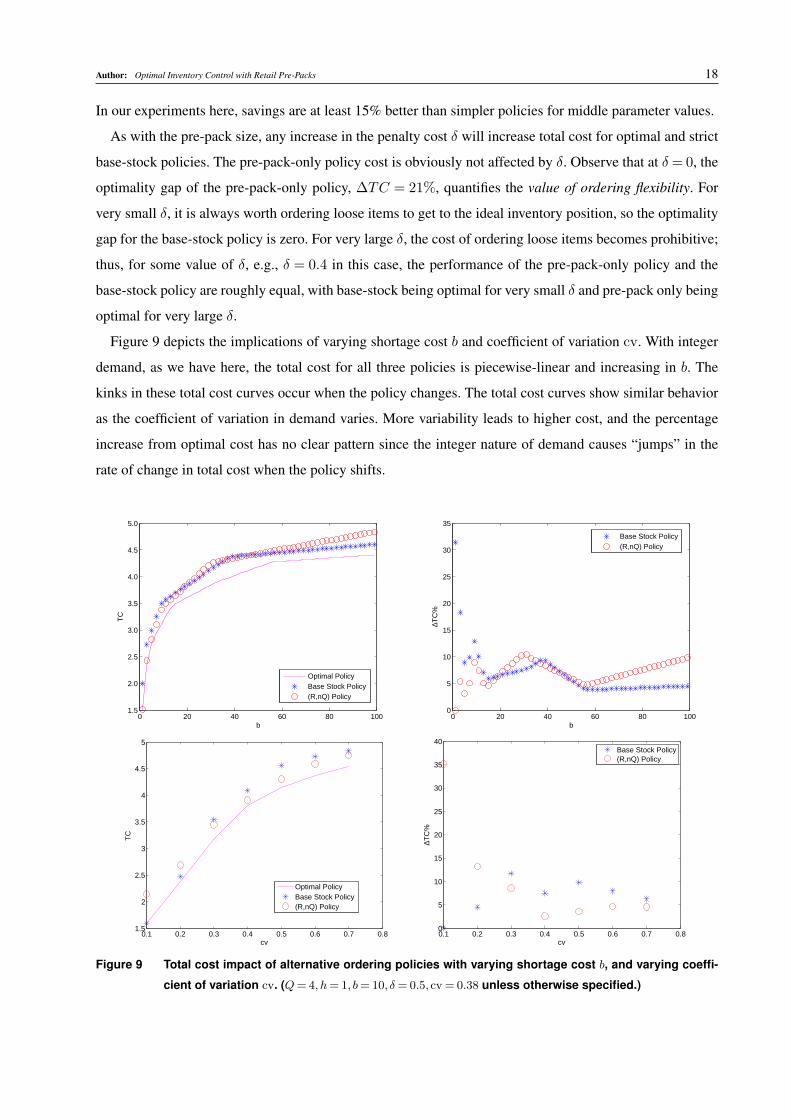
Figure 9 depicts the implications of varying shortage cost b and coefficient of variation cv. With integer

demand, as we have here, the total cost for all three policies is piecewise-linear and increasing in b. The

kinks in these total cost curves occur when the policy changes. The total cost curves show similar behavior

as the coefficient of variation in demand varies. More variability leads to higher cost, and the percentage

increase from optimal cost has no clear pattern since the integer nature of demand causes “jumps” in the

rate of change in total cost when the policy shifts.

0 20 40 60 80 1001.5

2.0

2.5

3.0

3.5

4.0

4.5

5.0

b

TC


0 20 40 60 80 1000

5

10

15

20

25

30

35

b

∆TC

%


0.1 0.2 0.3 0.4 0.5 0.6 0.7 0.81.5

2

2.5

3

3.5

4

4.5

5

cv

TC


0.1 0.2 0.3 0.4 0.5 0.6 0.7 0.80

5

10

15

20

25

30

35

40

cv

∆TC

%


Figure 9 Total cost impact of alternative ordering policies with varying shortage cost b, and varying coeffi-

cient of variation cv. (Q= 4, h= 1, b= 10, δ= 0.5, cv = 0.38 unless otherwise specified.)


6. ConclusionsIn this research, we study an inventory control problem where a retail store has the option of ordering

both pre-packs and individual units. For the single-SKU case, we show that, under certain conditions, the

optimal policy for a single period is to order into a band, ordering as few individual units as possible. The

policy is either (R,nQ) or base-stock policy for extreme cases. For the multi-period case with Q-modular

demand, we show that the band structure still holds by virtue of the Q-periodicity, and that the steady-state

distribution of the target inventory position possesses a semi-uniform structure. These structural properties

not only significantly reduce the computational efforts for the optimal policy, but also greatly facilitate

the development of effective approximations. For the multi-SKU case, the optimal policy, though more

complicated, is structurally similar to the single-SKU band policy. We further characterize the impact of

demand correlation on inventory control and pre-pack design. In contrast to the single-SKU case, the pre-

pack-only policy is no longer optimal because of its inability to control the rising demand disparity across

multiple SKUs. To control such disparity and total cost, the firms should pack together more positively

correlated items.

Our numerical experiments on the policy sensitivity and performance comparison lend insight to effective

inventory management with pre-packs. For the tests on the 2-SKU case, we find that pre-packs can be cost

effective for managing stable and positively correlated demand streams, especially when handling savings

are significant. Since the optimal policy may be difficult to implement, we compare the performance of the

optimal policy to two simple policies—strict base-stock and pre-pack only—in the single-SKU setting. For

extreme values of pre-pack size and incremental per-unit handling cost, one of these two policies performs

well; for moderate values, the cost increase associated with using these simpler policies can be substantial.

This paper has addressed how a firm could control inventory given a pre-pack. Although our numerical

study sheds some lights on the effects of pre-pack size and demand correlation, we have not explicitly

addressed the problem of how the pre-packs should be designed in general. Such a design problem would

require the specific relationship between handling savings and the size of the pre-pack; e.g., a larger pre-

pack would equal less inventory flexibility but presumably greater handling savings. Pre-pack design also

depends on the demand profile of the products involved, potentially across multiple stores. For example,

dynamic demand substitution creates positive correlation in demand when a stockout in one item transfers

the demand to another related item; umbrella branding is also likely to generate complementary demands

where the popularity in one product increases the demand in another product under the same brand.

Appendix

Convexity Lemma

The following lemma gathers the relevant properties of convex functions. Its proof can be found in Boyd and Vanden-

berghe (2004) and Topkis (1998).

LEMMA 1 (Convexity). (a) Define h ◦ g(x) = h(g1(x), . . . , gm(x)), with h : Rm → R, gi : Rn → R, i =

1, . . . , n. Then h ◦ g(x) is convex if h is convex and nondecreasing in each argument, and gi is convex for each i.


(b) If h: Rm →R is a convex function, then h(Ax+ b) is also a convex function of x, where A∈Rm×Rn, x∈Rn,

and b∈Rm.

(c) Assume that for any x∈Rn, there is an associated convex set C(x)⊂Rm and

{ (x, y) : y ∈C(x), x∈Rn } is a convex set. If h(x, y) is convex and the function g(x) ≡ infy∈C(x) h(x, y) is well

defined, then g(x) is convex over Rn.

(d) If f(x) and g(x) are convex on X and α,β > 0, then αf(x)+βg(x) is convex on X .

(e) Assume that F (ξ) is a distribution function on Y . Assume also that f(x, ξ) is convex in x on a lattice X for

each ξ ∈ Y , and integrable with respect to F (ξ) for each x∈X . Then g(x)≡∫Y

f(x, ξ)dF (ξ) is convex in x on X .

Proof of Lemma 2

(a). By the definition of Z and the convexity of [δ(I − y)+G(I)] in I , we have, for y <Z,

H(y) =minI≥y

[δ(I − y)+G(I)] = δ(Z − y)+G(I),

and, for y≥Z,

H(y) = δ(y− y)+G(y) =G(y).

Hence

H(y) =

{δ(Z − y)+G(Z), if y <Z,

G(y), if y≥Z.(21)

Taking the derivative at y = S yields H ′(S) = G′(S) = 0.7 This along with the convexity of H(y) shows that S =

argminy H(y).

(b). The inequalities R ≤ S ≤ R + Q follow from the convexity and coerciveness of H and H ′(S) = 0. The

inequality Z ≤ S holds because G′(·) is increasing, and H ′(Z) =G′(Z) =−δ < 0 =G′(S).

Proof of Theorem 1

(a). First, we argue that the optimal pre-pack decision is y∗ = y(x) ∈ (R,R +Q]. Indeed, by the convexity of H ,

H(y) ≥ H(y(x)) for any pre-pack position y ∈ (−∞,R] ∪ [R + Q,∞). Second, having arrived at y = y(x), it is

not optimal to order any loose if R ≥ Z, because ∂∂I[δ(I − y(x))) + G(I)] > 0 (by the convexity of the function

[δ(I − y(x)))+G(I)] in I and y(x)>R≥Z). Thus I∗ = y(x).

(b). Suppose Z >R. By Lemma 2.(b) we have R<Z ≤R+Q. Depending on the post-prepack-ordering position

y(x), we have two cases for loose decision I∗. If y(x) ∈ (R,Z], then H(y(x)) = δ(Z − y(x)) +G(Z) by (21); i.e.,

I∗ =Z. If y(x)∈ (Z,R+Q], then H(y(x)) =G(y(x)) by (21); i.e., I∗ = y(x). This completes the proof of part (b).

(c). If δ = 0, by (5) and (6), loose target Z and pre-pack target S coincide. By (5), base-stock policy S is optimal

for V (x) =min(y,I) {G(I) : y= x+nQ,n∈Z+, I ≥ y }=minI≥xG(I).

Proof of Theorem 2

It suffices to show that V (x) = V (x−Q), ∀x≤R+Q for three cases.

Case 1: Z ≤R and δ > 0. For x≤R+Q, we have

V (x) =

{G(y(x)+Q), y(x)≤R

G(y(x)), y(x)>Rby Theorem 1.(a)

=

{G(y(x−Q)+Q), y(x−Q)≤R

G(y(x−Q)), y(x−Q)>Rby Q-periodicity of y(x) in (9)

= V (x−Q). by Theorem 1.(a)

Case 2: Z >R and δ > 0. This can be similarly established by using Theorem 1.(b) and the Q-periodicity of y(x).

Case 3: δ= 0. The base-stock policy is optimal and we have V (x) =G(S) = V (x−Q) for x≤R+Q.

7 For a convex function f we use its maximal subgradient as its derivative at each x.


Proof of Lemma 3

Since ξQ ∼U [0,Q− 1], for I ≤R+Q, we have

EV (I − ξ) =∑ξ

f(ξ)V (I − ξ)

=

Q−1∑i=0

∑{ ξ:ξQ= i}

f(ξ)V (I − ξ)

=

Q−1∑i=0

∑n∈Z+

f(i+nQ)V (I − (i+nQ))

by ξ = ξQ +nQ and ξQ = i

=

Q−1∑i=0

∑n∈Z+

f(i+nQ)

·V (I − i) by Q-periodicity of V

=1

Q

Q−1∑i=0

V (I − i)∑n∈Z+

f(i+nQ) =1

Qby (13)

=1

Q

Q∑i=1

V (i), by Q-periodicity of V

where the last term 1Q

∑Q

i=1 V (i) is a constant.

Proof of Theorem 3

(a)-(c) Observe that the analysis in §3.1 relies on the convexity of G(I). Consequently, if we can show the convexity of

G(I) = hE(I−ξ)++bE(ξ−I)++βEV (I−ξ), then all the analysis in §3.1 applies. Since hE(I−ξ)++bE(ξ−I)+

is convex in I , it suffices to show the convexity of EV (I − ξ). However, Lemma 3 along with the hypothesis of

Q-periodicity from part (d) imply that EV (I − ξ) is a constant, and therefore convex for I ≤B+Q.

(d) The proof of this part parallels that of part (d) in Theorem 1.

Proof of Theorem 5

Let E ≡ {Z,Z +1, . . . ,R+Q } be the set of the target inventory positions. Assume Z > R. For demand ξ with

probability function f , we first define the set Ein for i∈E:

Ein ≡ i−E+nQ= { i− j+nQ : j ∈E }= [i−R−Q+nQ, i−Z +nQ]∩N. (22)

Thus, for each given inventory i, demand values can be classified into two sets: ∪nEin is the set of demand values such

that it requires only pre-packs to get into E after fulfilment of ξ, while (∪nEin)c is the set of demands that requires

ordering both pre-packs and loose. Then the transition probability pij can be computed as:

pij = P { ξ ∈∪nEin : ξ = nQ+ i− j }=∞∑

n=0

f(nQ+ i− j), if j =Z (23)

pij = P { ξ ∈ (∪nEin)c }+P { ξ = i−Z +nQ }= 1−

Q∑l=Z+1

∞∑n=0

f(nQ+ i− l), if j =Z (24)

For a given policy π, P = [pij ] is its associated Markov matrix. Denote a∆ =∑∞

n=0 f(nQ+∆), di = 1−Q∑

j=Z+1

ai−j .

Therefore,

pij =

{ai−j , if j =Z

di, if j =Z.(25)


Transition matrix P becomes

P =

dZ a−1 a−2 . . . aZ−(B+Q)

dZ+1 a0 a−1 . . . aZ+1−(B+Q)

dZ+2 a1 a0 . . . aZ+2−(B+Q)

......

.... . .

...dB+Q aB+Q−Z−1 aB+Q−Z−2 . . . a0

. (26)

The distribution ϕ of I is the solution to the balance equation (27) and the normalization equation (28):

ϕ= ϕ ·P (27)∑I

ϕ(I) = 1. (28)

Since ξQ ∼U [0,Q− 1], the following statements hold:

ai = aj = a= 1/Q, di = dj = d= 1− (B+Q−Z)a= (Z −B)/Q, ∀i , j ∈E. (29)

Then the transition matrix P can be simplified as:

P =

d a . . . ad a . . . a...

.... . .

...d a . . . a

(30)

ϕ =(

Z−BQ

, 1Q, . . . , 1

Q

)is a solution to (27) and (28) with matrix form (30). Furthermore, for irreducible Markov

Chains, the solution is unique. Hence, ϕ follows a semi-uniform distribution with mass Z−BQ

at point Z, and mass 1Q

at other points.

Proof of Theorem 6

(a). We first show the optimal pre-pack decision is y∗ = y(x) ∈ (Rℓx ,Rℓx +Q]. Indeed, for any y = x + n′Q ∈

(−∞,Rℓx ]∪ (Rℓx +Q,∞), we have H(y) =H(x+n′Q)≥H(Rℓx) =H(Rℓx +Q), where the inequality follows

from the convexity of hx(t) =H(x+ tQ) on line ℓx. Thus y∗ = y(x).

Now we show the optimality of the loose decision I∗ in (20). Given y∗ = y(x), the optimal loose decision I∗i for

SKU i only depends on yi(x), because the optimization is separable in the following sense:

maxI≥y(x)

[δδδ · (I−y(x))+G(I)] =k∑

i=1

maxIi≥y

i(x)

[δi(Ii − yi(x))+Gi(Ii)]. (31)

The same argument in the proof of Theorem 1.(b) establishes the optimality of I∗i in (20).

(b). The Q-periodicity of V (x) comes from the facts the optimal policy is prescribed by y(x) and that y(x) is

Q-periodic.

Proof of Theorem 7

(a). We prove the 2-SKU case in detail. The general k-SKU case follows the same line of argument by picking any

two distinct SKUs.

Let Eξi = µ, var(ξi) = σ2, i = 1,2, and ρ < 1. Let Di(τ) be the cumulative demand for SKU i over the initial

τ periods, and S(τ) the cumulative supply over the same τ periods. For sufficiently large τ , by the Central Limit

Theorem, Di(τ)∼N (τµ, τσ2), ∆τ ≡D1(τ)−D2(τ)∼N (0,2τ(1−ρ)σ2). Let m≡min{h1, h2, b1, b2}. Under the

pre-pack-only policy, the period τ cost is

Gτ (Iτ ) =∑2

i=1

[hiE(Ii,τ − ξi,τ )

+ + biE(ξi,τ − Ii,τ )+]

Ii,τ and ξi,τ are for SKU i in period τ

≥mE|D1(τ)−S(τ)|+mE|D2(τ)−S(τ)| by the law of conservation and |x|= x+ +x−


≥mE∣∣(D1(τ)−S(τ)

)−(D2(τ)−S(τ)

)∣∣ the triangle inequality and the linearity of E[·]

=mE|∆τ |

≥mE[ |∆τ |1{|∆τ |> 2στ} ] since E[ |X| ] =E[ |X|1A ] +E[ |X|1Ac ]≥E[ |X|1A ]

≥m · (2στ ) ·Pr{|∆τ |> 2στ} since r.v. |∆τ |> 2στ on set {|∆τ |> 2στ}

= 0.091m√2τ(1− ρ)σ2, since ∆τ ∼N (0,2τ(1− ρ)σ2) and Pr(|Z|> 2) = 0.0455

which implies the per-period cost Gτ (Iτ )→+∞ as τ →+∞. Hence the pre-pack-only policy cannot be optimal.

(b). By part (a) and ρis > ρjs, the pre-pack (i, s) has stochastically smaller demand disparity than the pre-pack

(j, s), since 2τ(1− ρjs)σ2 < 2τ(1− ρis)σ

2. For any given policy, this implies smaller total cost for pre-pack (i, s).

ReferencesAndersson, J., S. Axsater, J. Marklund. 1998. Decentralized multiechelon inventory control. Production and Opera-

tions Management 7 370–386.

Axsater, S. 2000. Exact analysis of continuous review (R, Q) policies in two-echelon inventory systems with compound

Poisson demand. Operations Research 48 686–696.

Berling, P., J. Marklund. 2006. Heuristic coordination of decentralized inventory systems using induced backorder

costs. Production and Operations Management 15 294–310.

Blackburn, J., G. Scudder. 2009. Supply chain strategies for perishable products: the case of fresh produce. Production

and Operations Management 18 129–137.

Boyd, S., L. Vandenberghe. 2004. Convex optimization. Cambridge university press.

Cachon, G.P. 2001. Exact Evaluation of Batch-Ordering Inventory Policies in Two-Echelon Supply Chains with

Periodic Review. Operations Research 49 79–98.

Chao, J., M. Chen, A. Deng, H. Miao, A. Newman, S. Tseng, C.A. Yano. 2005. Safeway designs mixed-product pallets

to support just-in-time deliveries. Interfaces 35 294–307.

Chao, X., S.X. Zhou. 2009. Optimal policy for a multiechelon inventory system with batch ordering and fixed replen-

ishment intervals. Operations Research 57 377–390.

Chen, F. 1998. Echelon reorder points, installation reorder points, and the value of centralized demand information.

Management Science 44 S221–S234.

Chen, F. 2000. Optimal policies for multi-echelon inventory problems with batch ordering. Operations Research

376–389.

Chen, S., J. Geunes, A. Mishra. 2012. Algorithms for multi-item procurement planning with case packs. IIE Transac-

tions 44 181–198.

Clark, A.J., H. Scarf. 1960. Optimal policies for a multi-echelon inventory problem. Management science 6 475–490.

Hadley, G., TM Whitin. 1961. A family of inventory models. Management Science 7 351–371.

Henig, M., Y. Gerchak, R. Ernst, D. F. Pyke. 1997. An inventory model embedded in designing a supply contract.

Management Science 43 184–189.

Litchfield, J., R. Narasimhan. 2000. Improving job shop performance through process queue management under

transfer batching. Production and Operations Management 9 336–348.


Morse, P.M. 1958. Queues, Inventory and Maintenance. John Wiley & Sons.

Parkinson, A., S. T. McCormick. 2005. Optimal replenishment with two delivery sizes. Manufacturing and Service

Operations Management Conference Presentation, Evanston, IL.

Puterman, Martin L. 1994. Markov decision processes: Discrete stochastic dynamic programming.

Smunt, T.L., J. Meredith. 2000. A comparison of direct cost savings between flexible automation and labor with

learning. Production and Operations Management 9 158–170.

Song, J. 2000. A note on assemble-to-order systems with batch ordering. Management Science 46 739–743.

Song, J.S., P. Zipkin. 1993. Inventory control in a fluctuating demand environment. Operations Research 41 351–370.

Topkis, D.M. 1998. Supermodularity and complementarity. Princeton Univ. Pr.

van der Vlist, P. 2007. Synchronizing the retail supply chain. Erasmus Research Institute of Management.

Veinott, A. 1965. The optimal inventory policy for batch ordering. Operations Research 13 424–432.

Zheng, Y., F. Chen. 1992. Inventory policies with quantized ordering. Naval Research Logistics 39 285–305.

optimal inventory control with retail pre-packs optimal inventory control with retail pre-packs 3...

Documents