1

Optimal Time-Average Cost for Inventory Systems with Compound Poisson Demands and Lost-sales

Michael N. Katehakis

Dept. of Management Science and Information Systems Rutgers Business School -- Newark and New Brunswick 1 Washington Park, Newark, NJ 07102 mnk@andromeda.rutgers.edu

Benjamin Melamed

Dept. of Supply Chain Management and Marketing Sciences Rutgers Business School -- Newark and New Brunswick 94 Rockafeller Rd. Piscataway, NJ 08554 melamed@business.rutgers.edu

Jim (Junmin) Shi

School of Management New Jersey Institute of Technology University Heights, Newark, NJ 07102 jmshi@gsu.edu

Supply contracts are designed to minimize inventory costs or to hedge against undesirable events

(e.g., shortages) in the face of demand or supply uncertainty. In particular, replenishment terms

stipulated by supply contracts need to be optimized with respect to overall costs, profits, service

levels, etc. In this paper, we shall be primarily interested in minimizing an inventory cost

function with respect to a continuous replenishment rate. Consider a single-product inventory

system in continuous review with constant replenishment and compound Poisson demands with

lost-sales. The system is subject to carrying costs and lost-sale penalties, where the carrying cost

is a linear function of on-hand inventory and the lost-sales penalty is incurred per lost-sale

occurrence as a function of lost-sale size. We first derive an integro-differential equation for the

expected cumulative cost until the first lost-sale occurrence. From this equation, we obtain a

closed form expression for the time-average inventory cost, and provide an algorithm for a

numerical computation of the optimal replenishment rate that minimizes the aforementioned time-

average cost function. In particular, we consider two special cases of lost-sales penalty functions,

2

constant penalty and loss-proportional penalty. We further consider special demand size

distributions, such as constant, uniform or Gamma, and take advantage of their functional form to

further simplify the optimization algorithm. In particular, for the special case of exponential

demand sizes, we exhibit a closed form expression for the optimal replenishment rate and its

corresponding cost. Finally, a numerical study is carried out to illustrate the results.

Keywords and phrases: Compound Poisson, integro-differential equation, lost-

sales, replenishment rate, time average cost.

3

1. Introduction

Supply contracts are designed to minimize inventory costs or to hedge against

undesirable events (e.g., shortages) in the face of demand or supply uncertainty

[Simchi-Levy et al. (2008)]. In particular, replenishment terms stipulated by

supply contracts need to be optimized with respect to overall costs, profits, service

levels, etc. In this paper, we shall be primarily interested in minimizing an

inventory cost function with respect to a continuous replenishment rate.

Production-inventory systems with constant replenishment rates are commonly

seen in both manufacturer industry and service organizations. Pharmaceutical

manufacturer and chemical industry, for examples, set up the production lines to

satisfy the incoming demands from customers. The setup time and cost are much

higher, which in turn allows no possibility of modification for the production line

thereafter. The tradeoff of an efficient production rate can be seen in two folds: If

the production rate is too high, after satisfying demands, there will be more

inventory hold in stock, which incurs more holding cost. On the other hand, if the

production rate is too lower, due to the inadequate on-hand inventory, potential

demands could not be filled immediately and thus incurs more penalty costs.

Therefore, decision on the number of production lines is exclusively important in

the stage of production planning. Such models can also be applied in service

organizations. Blood bank and food bank, for examples, are replenished at a

deterministic rate and face random demands. From managerial perspective,

selecting the right replenishment rate is one of the critical managerial decisions.

Consider a continuous-review single-product inventory system with continuous

replenishment and compound Poisson demands, subject to a lost-sales rule. In

this system, unsatisfied demand can be partially fulfilled from the on-hand

inventory (if any) and the excess demand (shortage) is lost. The excess demand

is referred to as the lost-sale size. Replenishment is continuous at a constant

(deterministic) rate, which can also be interpreted as a production rate. The

system incurs two types of costs: carrying cost and lost-sales cost. A carrying cost

is incurred as a function of the inventory on hand. A lost-sales cost is imposed at

4

each loss occurrence. The objective of this paper is to formulate and optimize the

time-average inventory cost with respect to the replenishment rate.

There is a large body of literature on managing inventory systems with compound

Poisson demands, that is, demand arrivals follow a Poisson process, and the

corresponding demand sizes follows an iid arbitrary distribution, independent of

arrivals. Early papers which study the inventory process include Richards (1975),

Thompstone and Silver (1975), Archibald and Silver (1978), Feldman (1978), and

Federgruen and Schechner (1983). Tijms (1972), Sahin (1979, 1983), and

Federgruen and Schechner (1983) generalize the compound Poisson assumption

to a general compound renewal processes, in which both the demand inter-arrival

times and demand sizes have arbitrary distributions. Presman and Sethi (2006)

provides a detailed literature review with a comprehensive reference list. The

aforementioned papers assume various replenishment policies, but exclude

continuous replenishment.

Production-inventory systems with constant replenishment and various demand

processes have been previously studied in the literature. Graves and Keilson

(1981) considers a one-product, one-machine production-inventory problem. The

demand process is governed by a compound Poisson process with exponential

demand sizes. The system is subject to a (r, R) policy with a constant

replenishment rate. The paper analyses the cost optimization problem as a

constrained Markov process using the compensation method. The optimal policy

is then obtained via a search of the policy space. Graves (1982) presents two

models for inventory systems with continuous production and perishable items.

For each of these models, the paper derives analytical expressions for the steady-

state distribution of system inventory, using a queuing-theoretic approach. The

steady-state results are then used to evaluate various system performance metrics.

Gullu and Jackson (1993) considers a one-product inventory problem with a

constant production rate and a demand process with stationary and independent

(i.e., time-homogeneous and additive) increments, and the replenishment policy is

produce-up-to-S. The paper derives the stationary distribution of the inventory

level by extending existing results for dam systems, and then optimizes the time-

5

average cost of the system, by exhibiting a closed form formula for the optimal

policy.

A number of papers study the derivation of optimal or near-optimal inventory

replenishment, which minimizes the time-average cost. Springael and

Nieuwenhuyse (2005) studies a lost-sales inventory model with a compound

Poisson demand process, in which replenishment lead times are negligible. On-

hand inventory is managed according to a (0, B*) policy, namely, when the shelf

inventory drops to 0, the retailer instantaneously gets a fixed amount of B* units

from the central stockroom as replenishment. The paper analyzes the time-average

cost of the system and provides a steepest-descent-based algorithm to calculate

the optimal B* parameter. In a similar vein, Minner and Silver (2007) study an

inventory system with compound Poisson demands and negligible replenishment

lead times. The paper formulates the optimization problem as a Markov-

decision-problem, which can be applied to inventory systems with a small number

of products. For a larger number of products, the paper proposes several heuristics

for the optimal reorder points and reorder quantities. .

Similarities between the mathematical formalisms of queueing and inventory

models had been observed at a fairly early stage in their development. The linkage

between those two areas has been studied by Prabhu (1965). However, from

managerial point of view, inventory performs and are treated differently from the

classical G/M/1 queue sever. For example, under lost-sales policy, the inventory

incurs no service time, no waiting time for customer demand since there is no

waiting queue of customers. From the perspective of revenue management, the

basic objective of inventory management is to minimize the (discounted or time-

average) inventory cost. For other related recent work in the broader area of

service systems we refer the reader to Li and Glazebrook (2010), Ivo et al. (2005),

Perry and Stadje (2003).

We are not aware of any previous work on stochastic models with continuous

replenishment. However, for a good recent survey of related Markovian demand

inventory models and theory, we refer the reader to Beyer et al. (2010) and

references therein. Accordingly, this paper makes a number of contributions to

6

the field of inventory systems with inventory system, continuous replenishment

and compound Poisson demands, subject to a lost-sales rule. The main

contributions of this paper are listed below:

i) A closed form expression for the time-average inventory cost of the system

is obtained in Theorem 2, Eq.(3.43), for arbitrarily distributed demand and a

general penalty function.

ii) A characterization of the optimal continuous replenishment rate that

minimizes the time-average inventory cost is derived in Theorem 3 for

general demand distributions and general penalty functions.

iii) An algorithm to numerically calculate the optimal replenishment rate is

presented in Eq. (5.3).

iv) Closed form expressions for the optimal replenishment rate and their

attendant costs are obtained for the case of exponential demand, for both

constant penalty and loss-proportional penalty functions.

v) We further consider special demand size distributions, such as constant,

uniform or Gamma, and take advantage of their functional form to further

simplify the optimization algorithm.

The rest of this paper is organized as follows. Section 2 introduces notation and

formulates the inventory model under study. Section 3 uses a renewal argument to

derive an integro-differential equation for the cost function until and including the

first lost-sale occurrence. From this equation, we obtain a closed form formula

for the time-average cost, expressed as a ratio of the conditional expected total

cost until the first lost-sale occurrence divided by the conditional expected time to

the first lost-sale, given zero initial inventory level. It also derives a closed form

expression for the time-average cost function. Section 4 investigates the existence

and uniqueness of the optimal replenishment rate which minimizes the

aforementioned cost function as well as asymptotic costs. Section 5 treats the

time-average cost optimization problem with general demand distribution and

studies some special cases: constant penalty and loss-proportional penalty. Section

6 contains three numerical studies that illustrate our results. Finally, Section 7

concludes this paper.

7

2. Model Formulation

Throughout the paper, we use the following notational conventions and

terminology. Let denote the set of real numbers. For any real number

x , max 0x x{ , }� . The indicator function 1{ }A is 1 if A is true, 0

otherwise. For a real function ( )f x , ( )f x denotes the right limit of ( )f x at

x . For a random variable X , let Xf x( ) ,

XF x( ) and 1

X XF x F x( ) ( )

denote respectively its probability density function (pdf), its cumulative

distribution function (cdf) and its complementary cdf, respectively. The Laplace

transform of a function f x( ) is defined by

0

zx

f z f z e f x dxL( ) = ( ) = ( ) .

If real functions ( )f x and ( )g x are defined on 0[ , ) , then the convolution

function of ( )f x and ( )g x is given by

0( ) ( ) ( )

u

f g u f u x g x dx .

Also, we assume the continuous compound interest rate, 0r is a given

constant. Hence, the present value of one unit cash flow at time t is r t

e .

In this paper, we shall make repeated use of the following relation

0 0

1 11 1( ) ( ) ( ) ( )zx zx

D D D DF z e F x dx e dF x f zz z

(2.1)

where the second equality follows from integration by parts.

2.1 The inventory process

The demand arrival stream : 0{ }i

A i t follows a compound Poisson process

with rate , where time 0 0 A by convention. Thus, the corresponding

sequence of interarrival times, : 1{ }i

T i t , where 1� �i i i

T A A have iid

exponential distributions. The corresponding demand sizes form an iid sequence

: 1{ }i

D i t with a common density function ( )Df x and common mean demand,

[ ]D

D , where demand i

D arrives at time i

A . Replenishment occurs

8

at a constant (deterministic) rate 0! . Throughout this paper, we assume the

stability condition

D. (2.2)

By Prabhu (1965), this stability condition implies that a lost sale occurs with

probability 1. Let 0{ ( ) : }I t t denote the right-continuous inventory

process, given by

10

� � �¦N t

i i iI t I t D L A

( )( ) ( ) ( )[ ] , (2.3)

where ( )N t is the number of demands arriving over 0( , ]t and

, , 1,2,...0, otherwise

­ � � ° ®°̄

i i iD I A t A i

L t( )

( )[ ]

(2.4)

is the lost-sales size (excess demand that cannot be satisfied from on-hand

inventory under the lost-sale rule) associated with the i -th demand arrival, and

zero, otherwise. Denote by I the infinite-horizon time-average inventory,

namely,

01

o ³lim

t

t

I I z dzt

( ) . (2.5)

Let 0{ : }i i be the sequence of loss occurrence times, given by

1inf : 0{ ( ) }i i-

t L t , (2.6)

where 0 0 . Let : 1,2,...{ }k

J k be the sequence of random arrival indexes

at which loss occurs, namely, k

JkA . Figure 1 illustrates the evolution of the

inventory process with lost-sales over an infinite time horizon.

Figure 1. A sample path of the inventory level process, { ( )}I t

9

Figure 2 depicts the detailed evolution of a sample path of the inventory process

in the interval 10 .

Figure 2. A sample path of the inventory level process in the interval 10

2.2 The inventory cost

The inventory cost under study is incurred by carrying costs and lost-sales

penalties. These cost components are described as below.

x Carrying costs. While there is inventory on hand, a carrying cost is incurred at rate h per unit time and per inventory unit. Accordingly, the carrying cost process : 0{ }H H t t t( ) is given by

0 ³

t

H t h I z dz( ) ( ) (2.7)

x Lost-sales penalties. Whenever  a  customer’s  demand cannot be satisfied from on-hand inventory, a penalty of the form w x( ) is incurred as a non-decreasing function of the lost-sale size, x , with the proviso that

0 0w( )= . In particular, we shall consider a linear penalty function (to be studied in Section 6 as a special case) of the form

0 0 1{ }xw x K K x�( )=1 , (2.8)

where 0 0K is a constant penalty per lost-sale occurrence, 1 0K is a

constant penalty per unit of lost-sales, and the two constants do not vanish

simultaneously. Accordingly, the penalty process : 0 t{ }W W t t( )

is given by

10

1 ¦N t

i iW t w L A

( )( ) ( ( )) (2.9)

The inventory cost process : 0{ }C C t t t( ) is given by

10 ¦³( )= + +

N t

i

t

iC t H t W t h I z dz w L A

( )( ) ( ) ( ) ( ( )) . (2.10)

The infinite-horizon time-average inventory cost is defined by

0ot

C t I uc

t

[ ( )| ( )= ]= lim . (2.11)

In a similar vein, the infinite-horizon time-average carrying cost is defined by

0ot

H t I uh

t

[ ( )| ( )= ]= lim , (2.12)

and the infinite-horizon time-average penalty by

0ot

W t I uw

t

[ ( )| ( )= ]= lim . (2.13)

Thus, we have

�c h w . (2.14)

3. Solutions for the Time-Average Cost Function

In this section we derive closed form expressions for the time-average cost

functions. Specifically, we first derive an integro-differential equation for the

conditional expected discounted cost function until and including the first lost-sale

occurrence, and then use it to solve for the time-average cost c . The main result

of this section is the closed form expression for the time average cost, c , which

is given by Theorem 2 in Subsection 3.4.

3.1 The function c To derive the time average cost function c we first consider the inventory cost

until and including the first lost-sale occurrence. It is given by

11 10

( )= +C h I z dz w L³ ( ) ( ( )) . (3.1)

Its expected value, conditional on 0( )=I u , is denoted by

1 0c u C I u( )= [ ( )| ( )= ]. (3.2)

11

Note that the inventory process over intervals of the form 1,i i� is a renewal

process and the corresponding incurred cost process can be regarded as a renewal

reward process. Consequently, by Theorem 3.6.1 in Ross (1996), with probability

1, the time-average cost in Eq. (2.11) is independent of the initial inventory level,

and given by

1

00 0

( )=

[ | ( )= ]

cc

I. (3.3)

Our objective is to obtain a formula for c , by deriving 0c ( ) and

1 0 0[ | ( )= ]I . To this end, we shall make use of the total discounted inventory

cost until and including the first lost-sale occurrence, given by

111 10

( )= + rrz

rC h I z e dz w L e

��³ ( ) ( ( )) (3.4)

and its associated conditional expected discounted cost function by

1 0r r

c u C I u( )= [ ( )| ( )= ] . (3.5)

We shall utilize the discounted quantities above as follows. To compute 0c ( ) ,

we shall use the fact that c u( ) may be obtained from r

c u( ) in Eq. (3.5) by

setting there 0=r , so that 0( )= ( )c u c u . Next, to compute 1 0[ | ( )= ]I u ,

define

1 0�r

rd u e I u( )= [ | ( )= ] . (3.6)

Note that setting 0=h and { 0}1x

w x( )= in Eq. (3.4) implies

( )= ( )r r

d u c u . (3.7)

Finally, we shall need the following lemma.

Lemma 1 Under the stability condition (2.2), the conditional expected time to the first lost-

sale occurrence is

1 00 ww r r

I u d ur

[ | ( )= ]= ( )| . (3.8)

Proof. To prove Eq. (3.8), write

12

1 1

1 1

1

0 | 0 | 00 00 0

| 0 | 00 00 0

|

lim lim ( | lim ( |

lim ( | lim ( |

o

� �

o o

� �

o o

w w ww w w

� �

�

³ ³

³ ³

rr

rt rt

I Ir r

rt rt

I Ir r

d u e f t u dt e f t u dtr r r

t e f t u dt t e f t u dt

t f

( ) ( )

( ) ( )

( )= ) = )

= ) = )

= 100

( | 0 ]�³ It u dt I u( ) ) = [ | ( )=

where the second equality holds by the Leibniz integral rule, while the fourth one holds by the Dominated Convergence theorem, because

1 1| 0 | 0( | ( |�rtI I

|te f t u t f t u( ) ( ))| )

such that 1 1| 0

0

( | 0 ]³ It f t u dt I u( ) ) [ | ( )= by Prabhu (1965). □

3.2 The Function r

c u( )

For any given initial inventory level 0u , and a time interval 0( , ]s , where

0s is small, consider the following disjoint events and the corresponding

discounted cost function, r

c u( ) .

(1) On the event 1{ }A s , the corresponding cost is

1

0

0

0r A s

t rz rs

r

s rz rs

r

s

s

s

C I u

e h u z e dz c u s e dt

e h u z e dz c u s e

{ }[ 1 | ( ) =

( ) ( )

( ) ( )

]

=

, (3.9)

where the first term in the sums above is the discounted carrying cost over

0( , ]s , and the second is the discounted residual cost over 1( ]s , since

1 1{ } { }A s s� .

(2) On the event 1{ }A s , the corresponding cost is

1 00{ }[ 1 | ( ) = ,t

r A s

s

C I u e M u t dt] ( ) (3.10)

where 1 0, [ | , ( ) =rM u t C A t I u( ) = ] is given by

13

0

0

, ( )

( ) ( )

+ ( ) ( )

D r

D

rz

u trt

rt

u t

t

M u t h u z e dz

e f x c u t x dx

e f x w x u t dx

( )

( )

(3.11)

So that

0, ( )+ ( )D Dr

u

M u f c u f x w x u dx( ) ( ) . (3.12)

Thus, adding Eqs. (3.9) and (3.10) yields

00( ) ( ) ( ) ,s rz rs t

r r

ss

c u e h u z e dz c u s e e M u t dt( )

(3.13)

Next, differentiating Eq. (3.13) with respect to s , and setting 0s , we have

0 0( ) ( ) ( ) ,r rh u r c u c u M uu

( ) . (3.14)

Finally, substituting Eq. (3.12) into Eq. (3.14) yields after rearranging terms

( ) ( ) ( ) ( ) ( )Dr rrc u r c u f c u g u

u, (3.15)

where

( )Du

g u h u f x w x u dx( ) ( ) . (3.16)

It is convenient to decompose the function above into 1 2( ) ( ) ( )g u g u g u ,

where

1( )g u hu , (3.17)

2( ) ( )D

u

g u f x w x u dx( ) . (3.18)

Thus, 1( )g u corresponds to the carrying cost component, while 2( )g u

corresponds to the lost-sales penalty component.

Next, we proceed to solve Eq. (3.15) for ( )rc u . To this end, we take Laplace

transform on both sides of that equation to get

0 0[ ( ) ( )] ( ) ( ) ( ) ( ) ( ),Dr r r rz c z c r c z f z c z g z z

(3.19)

Rearranging and simplifying the above equation yields

14

0 0[ ( ) ] ( ) ( ) ( ),D r rf z z r c z c g z z , (3.20)

Denoting the first factor in Eq. (3.20) as the auxiliary function

( ) ( )r Dz f z z r , (3.21)

Eq. (3.20) can now be written as

0 0( ) ( ) ( ) ( ),r r rz c z c g z z , (3.22)

For ease of exposition, denote the first root of the equation 0( )r z by ( )r

and the second root by ( )r where ( ) < ( )r r , provided they exist.

The following lemma summarizes some key properties of the equation

0( )r z .

Lemma 2

For any 0r , the equation 0( )r z has two distinct roots, ( )r and ( )r

as follows:

(a) If 0r , then 0 0( ) and 0 0( ) . (b) If 0r , then 0( )r and 0( )r .

Proof. We first prove that the function ( )r z is convex by computing its first

and second derivatives,

0( ) ( )D

zx

r z xe f x dxz

, (3.23)

22

2 0( ) ( )D

zx

r z x e f x dx

z

. (3.24)

Since the case of zero demand with probability 1 is precluded, it follows from Eq.

(3.24) that 2

20( )r z

z

. (3.25)

To prove part (a) for 0r , we have 0 0 0( ) , namely, zero is a root of

0 0( )z . It remains to show the existence of exactly one more positive root.

First, note that 00 0( ) |zzz

by Eqs. (3.23) and (2.2). Therefore, there

exists 0'z such that 0 0( ')z But since 0( ) , there must be a

positive root. Second, we prove by contradiction that there cannot be more than

15

two roots. Otherwise,  by  Rolle’s  Theorem,  there must be more than one *z such

that 0 0( *)zz

. This contradicts the fact that that there is at most one *z

such that 0 0( *)zz

by Eq. (3.25), thereby establishing part (a).

To prove part (b) for , 0 0( )r , ( )r and ( )r .

Consequently, there must be at least one positive root and one negative root for

0( )r z . An argument similar to that in part (a) establishes that there cannot be

more than two roots as required. □

Figure 3 illustrates the key features of the function ( )r z and the root structure

for the equations and 0( )r z .

Figure 3. Illustration of the function and its root structure

In particular, for 0r , we denote

0( ) .

In view of Lemma 2, we can write,

0( )Df , (3.26)

and generally,

0r

( )r z

16

( )Df r . (3.27)

where ( )r is the unique positive root to Eq. (3.27), and 0( ) is the

unique positive root to Eq.(3.26), and it follows that 0

lim ( )r

ro

, as illustrated in

Figure. 3.

Lemma 3

(a) For 0 and ( ) ,

( )DF . (3.28)

(b) For , the mapping ( ) is strictly monotone decreasing. Proof. To prove part (a), note first that by Eq. (3.26),

1 ( )Df

, (3.29)

Eq. (3.28) now follows by Eqs. (2.1) and (3.29).

To prove part (b), we differentiate Eq. (3.28) with respect to , yielding

01

( )( ) ( )

x

Dx e F x dx .

The equation above implies 0( ) since the integral on the right hand side is

strictly positive for all , which in turn implies the result. □

Corollary 1

0limo

. (3.30)

where .

Proof. Sending 0p on both sides of Eq. (3.28) implies 0

lim 0o

( ( ))D

F ,

which in turn implies

0limo

( ) . (3.31)

Furthermore, Eq. (3.26) can be written as

0

0

( )

17

( )Df . (3.32)

The proof immediately follows via sending in Eq. (3.32) and the fact

0lim ( ) 0o

Df . □

We are now in a position to derive a closed form formula for 0( )rc .

Lemma 4

0 ( ( ))( )r

g rc . (3.33)

Proof. The result follows by setting ( )z r in Eq. (3.22) and noting the first

term vanishes by Lemma 2. □

Corollary 2

0 ( )( )

gc . (3.34)

Proof.

Follows from Eq. (3.33) and the fact that . □

3.3 The Function ( )r

d u Consider the special case 0h and 0{ }xw x( ) = 1 . Then, Eq.(3.16) becomes

( ) ( ) ( )D D

u

g u f x dx F u

and consequently by Eq. (3.15) satisfies the following integro-

differential equation,

( ) ( ) ( ) ( ) ( )r r D r D

d u r d u f d u F uu . (3.35)

The following lemma provides a closed form formula for 0rd ( ).

0p

0lim ( )r

ro

( )r

d u

18

Lemma 5

0 1( )( )r

rd

r. (3.36)

Proof. Set and in Eq. (3.33), which becomes

0r Dd F( ) ( ) . (3.37)

in view of Eq. (3.7). Using Eq. (2.1), we can rewrite Eq. (3.37) as

0

( )( )r

Dfd (3.38)

Furthermore, by Eq. (3.27), the numerator of Eq. (3.38) can be written as

( )Df r . (3.39)

The result now follows by substituting Eq. (3.39) into Eq. (3.38). □

Theorem 1

110 0[ | ( )= ]=I . (3.40)

Proof. In view of Eqs. (3.8) and (3.36), we have

1 0

20

00 0 0 lim 1

1 1 1 lim

[ | ( )= ]= ( )|( )

= ( ) =( ) [ ( )]

rr

r

r

rI d

r r r

rr

r r

o

o

ª ºw

�« »w ¬ ¼­ ½

c�® ¾¯ ¿

ww

Here, the first equality holds by Eq. (3.8) at 0=u , the second equality holds by

Eq.(3.36). The fourth equality is due to the fact that 20lim 0( )

[ ( )]r

rr

roc , and to

show that it suffices to prove that 20

1lim ( )[ ( )]r

rro

c exists and is finite. To see

that, we first note that 2 2

0lim[ ( )]r

ro

. Secondly, since ( )r r is a one-to-one

mapping by Lemma 2 and Eq. (3.27), one has 0

1limlim

( )=( )r

rro

o

cc

.

Furthermore, by Eqs. (3.21) and (3.27), one has

0h 0{ }xw x( ) = 1

19

( ) ( ) zrr zz

ww

.

Therefore, by continuity of ( )r zz

ww

at z , shown in the proof for Lemma

2, we have

0lim 0( ) ( ) zr zz

ww

, (3.41)

again by the proof for Lemma 2. We conclude that is finite as

claimed □

Let denote the fill rate (fraction of demand arrivals that can be immediately

satisfied from inventory on hand) in our system, and let the lost-sale rate be

denoted by 1= .

Corollary 3

( )=Df . (3.42)

Proof. We have

1

1 ( )0 0

[ ]= = =

[ | ( )= ] D

Af

I,

where the first equality follows from [Ross (1996), Theorem 3.4.4], the second

follows from Eq. (3.40), and the third equation holds by Eq. (3.32). The result

above is equivalent to Eq. (3.42). □

We point out that for 0 , 110 0 �[ | ( )= ]=I clearly holds (that is, in a

system without replenishment, started with zero initial inventory, each demand

arrival results in a lost sale, and consequently, the mean time between losses is 1� ). Indeed, this result is obtained by sending 0p on both sides of Eq.

(3.40) and substituting Eq. (3.30) into Eq. (3.40).

3.4 Closed form expression for c

20

1lim ( )[ ( )]r

rro

c

20

The following theorem provides computable representations for the infinite-

horizon time-average total cost and its components (carrying cost and lost-sales

penalty).

Theorem 2

( )=c g , (3.43)

1( )=h g , (3.44)

2 ( )=w g (3.45)

where .

Proof. To prove Eq. (3.43), substitute Eqs. (3.34) and (3.40) into Eq. (3.3).

Eqs. (3.44) and (3.45) readily follow by noting that 1 2�g=g g implies

1 2�g=g g . □

Corollary 4

=h

h , (3.46)

1=I . (3.47)

Proof. Note that 1 2( ) hg z

z by Eq. (3.17). Eq. (3.46) now readily follows by

substituting 1( )g into Eq. (3.44). Finally, Eq. (3.47) follows immediately

from Eq. (3.46) by noting that the inventory time average is equivalent to the

time-average carrying cost with =1h . □

Since our model does not have a base-stock level, excursion of the inventory

process can generally reach arbitrary large levels. The following lemma provides

a bound on the probability of the inventory level exceeding a given value.

Lemma 6

For a given replenishment rate, , consider the corresponding inventory process

in the steady state regime. Then, for 0s ,

( )

21

1{ ( ) }P I t s

s, 0t . (3.48)

Proof. By Markov inequality [Karr (1993)],

[ ( )]

{ ( ) }I t I

P I t ss s

The result now follows from Eq. (3.47). □

4. Cost Function Properties In this section, we study properties of the cost function c given by Eq. (3.43)

and its components, h and w . To this end, we first provide some asymptotic

results of the cost functions, and then demonstrate the existence and uniqueness of

its minimum.

We first rewrite Eq. (3.43) as

> @ > @( ) (0+) ( ) c c� �= = [ ]c g g g w D( )L L , (4.1)

where the first equality holds by a property of the Laplace transform [cf. Widder

(1959)], the second equality follows from Eq. (3.16), and

2 0( ) ( ) ( ) ( ) ( ) ( )D D

u

g u h g u h f x w' x u dx f u w . (4.2)

Lemma 7

(a) h is monotone increasing and convex in 0 , and has the following

asymptotes

0lim 0h = ` (4.3)

lim =h (4.4)

(b) w is monotone decreasing and concave in 0 , and has the following

asymptotes

0lim = [ ]w w D( ) (4.5)

lim 0=w (4.6)

(c) c has the following asymptotes

22

0lim = [ ]c w D( ) (4.7)

lim =c (4.8)

Proof. Part (a) readily follows from Eq. (3.46). To prove part (b), we first prove

Eq. (4.5) by writing

2 20 0lim lim lim= ( ) = ( ) = [ ( )]

u

w g g u w D .

Here, the first equality follows from Eq. (3.45) and the monotone decreasing

relation between and exhibited in Eq. (3.28); the second equality holds by

the initial value theorem of the Laplace transform [cf. Widder (1959)]; and the

third equality holds by Eq.(3.18).

Next, to prove Eq. (4.6) we write

2 20lim lim lim= ( ) = ( ) =

u

w g g u .

Here, the first equality holds by Eq. (3.45) and the decreasing monotone relation

between and exhibited in Eq. (3.28); the second equality holds by the final

value theorem of the Laplace transform [cf. Widder (1959)]; and the last equality

holds by Eq.(3.18).

We next show that the monotonicity and concavity of w follow from its first

and second derivatives, respectively. To this end, we write

> @2 2 2 20( ) ( ) (0+) ( )c c� �³ x

w g g g e g x dx w D= = = [ ( )]L , (4.9)

where the first equality holds by Eq. (3.45); the second equality holds by a

property of the Laplace transform (Widder 1959); the first term in the third

equality holds by definition; and the second term in the third equality holds by Eq.

(3.18). Differentiating Eq. (4.9) now yields

20( ) 0w c

w ³ xw xe g x dx= (4.10)

22

22 0( ) 0w c

w ³ xw x e g x dx= (4.11)

Here, we use the fact that Eq. (3.18) implies

2 0 0D D

u

g u f x w' x u dx f u w( ) ( ) ( ) ( ) ( ) , (4.12)

23

since  the  equality  holds  by  the  generalized  Leibniz’s  integral  rule,  and  the  

inequality holds in view of Df u( ) 0 and the fact that the inequalities

0w w' x( ), ( ) 0 hold by assumption. This completes the proof for part (b).

Finally, Eqs. (4.7) and (4.8) follow by adding Eq. (4.3) to Eq. (4.5), and adding

Eq. (4.4) to Eq. (4.6), respectively. □

We are now at a position to study the existence and uniqueness of the minima of

c . We mention that it is straightforward to prove the existence of minima;

however the proof of uniqueness is much challenging. Still, we can prove

uniqueness for some important cost functions. The following Lemma provides

results for the case of 0 0( )w .

Lemma 8

For 0 0( )w ,

(a) if 0h , then c attains a unique minimum at * [ ]D , where * 0 ;

(b) if

0 [ ]h w' D( ) , (4.13)

then c has a unique and finite minimum at * *( )DF , where * 0 ;

(c) if 0[ ]h w' D( ) , then c attains a unique minimum at 0* ,

where * .

To prove Lemma 8, we shall make use of the following result (see Appendix for a

proof).

Proposition 1

Let f x( ) be a continuous function, not identically zero, satisfying

00f x dx( ) , (4.14)

and there exists a constant 0 0x such that 0( )f x for 00 x x , and

0( )f x for 0x x . Then, 0f z( ) if and only if 0z .

24

Proof for Lemma 8 If 0 0( )w , then Eq. (4.2) implies

( ) ( ) ( ) ( )Du

g u h f x w' x u dx R u , (4.15)

where ( )R u is an increasing function of u . Furthermore, Eqs. (4.1) and

(4.15) jointly imply

( ) �= [ ]c R w D( ) . (4.16)

Eq. (4.16) shows that minimizing c in is equivalent to minimizing ( )R

in .

To prove Part (a), observe that 0h implies that 0( )R u because ( )w x is

a non-decreasing function (of the loss) by assumption (see Section 3), and

consequently ( ) R is strictly increasing. Part (a) now follows since ( )R

attains a unique minimum at * 0 .

To prove Part (b), the existence of the minimum follows from the continuity of

c and Part (c) in Lemma 7. It remains to prove the uniqueness of the minimum.

To this end, differentiate Eq. (4.16) with respect to , and set the derivative to

zero, yielding

0 00( ) x

c xe R x dx f x dx( ) ( ) . (4.17)

where ( ) xf x xe R x( ).

Next, Eq. (4.15) implies

lim 0( )u

R u h . (4.18)

Furthermore, the assumption [ ]h w' D( ) and Eq. (4.15) imply

0 0( )R . Using the two limits above and the continuity and monotonicity of

( )R u , it follows that there exists a constant 0 0u , such that 0( )R u for

00 u u , while 0( )R u for 0u u . Consequently, we conclude that

for any 0 , one has 0( )f x for 00 u u , while, 0( )f x for

25

0u u . Letting * denote a solution of Eq.(4.17), we next prove its uniqueness

by contradiction. Suppose there exists another solution of Eq.(4.17), such

that without loss of generality, * . Then, by Eq. (4.17)

0 00*

*)(( ) ( )xc f x dx e f x dx( ) .

In view of Proposition 1, we must have 0* in contradiction to the

assumption * , which completes the proof for Part (b).

Finally, to prove Part (c), if h w' D[ ]( ) , then 0( )R u by Eq. (4.15). It

follows that ( ) R is non-increasing, which completes the proof for Part (c). □

Figure 4 illustrates a typical as function of the original domain variable (the

replenishment rate, ), and a Laplace domain variable (the positive root, );

recall that and are related by Eq. (3.28).

Figure 4. A typical as function of (left) and (right)

In the following discussion, we shall derive the unique optimal replenishment

rate.

5. Optimal Replenishment Rate In this section, we optimize the time-average cost of Eq. (2.11) with respect to

the replenishment rate, . We first provide a general structural result for the

c

c

26

optimal replenishment rates, * , and then we study some special cases. Note

that we admit the possibility of multiple optimal replenishment rates.

Theorem 3

The optimal replenishment rates for Eq. (2.11) are given by

* *( )DF , (5.1)

where *

0argmin ( )= { }g . (5.2)

Proof. In view of Eq. (3.43), minimizing ( ) ( ( ))=c g with respect to is

equivalent to minimizing ( ) =c g with respect to the nonnegative variable

. To this end, we first compute Eq. (5.2), namely, perform optimization on

( ) =c g in the Laplace domain to find the optimal values * . Next, by

Lemma 3(b), is 1-1, and consequently, we can invert each * *( )

via Eq. (5.1) to obtain the corresponding optimal replenishment rate, * . □

The minimum values, * , given in Eq. (5.2), can be calculated in several ways.

A straightforward but relatively time consuming method is global search.

However, when * is unique, the availability of derivatives of ( )c with

respect to allows  us  to  apply  the  relatively  fast  Newton’s  Method,  where  

successive approximations of the minimum are given by the iterative scheme,

2

2

+1

( ), = 0,1,

( )

wwww

n

nn

n

c

n

c

= . (5.3)

We next proceed to study production-inventory systems with specialized lost-

sales penalty structures, specifically the constant lost-sales penalty and the loss-

proportional penalty. Under each penalty structure, we study the optimal average

costs, subject to particular demand distributions, such as constant, uniform,

Exponential and Gamma distributions.

( )

27

5.1 Constant Lost-Sales Penalty In this case, 001{ }xw x K( ) = , where 0 0K is a constant. Then, Eq. (3.16)

becomes

0 0( ) ( ) ( )D Du

g u hu K f x dx hu K F u , (5.4)

and the corresponding Laplace transform is given by

2 20 01 ( )( ) ( ) �

� �= = D

D

f zh hg z K F z K

z z z,

where the second equality holds by Eq. (2.1). In view of Eq. (3.43), we now

have

00( ) 1 ( )ª º� � �¬ ¼= =D

h hc g K f , (5.5)

where the last equality holds by Eq. (3.29). By Eq. (5.2), the optimal * is

given by

*

00 ( )

!

­ ½ �® ¾

¯ ¿argmin

D

hK f . (5.6)

We mention that * is a monotonically decreasing function of 0K

h. To see

this, Eq. (5.6) can be rewritten as * 0

0

1 ( )­ ½ �® ¾

¯ ¿argmin

D

Kf

h, so that the

derivative of the rewritten objective function with respect to 0K

h is

( ) 0� �Df , which implies the result. It follows that * is a monotonically

increasing function of 0K

h, because is a monotonically decreasing function

of 0K

h, while ( ) is monotonically decreasing in .

Table 1 exhibits the expressions for * , * and *c for selected demand

distribution with detailed derivations given in Appendix.

Table 1. Optimal Quantities for Production-Inventory Systems Subject to Constant Penalty and Various Demand Distributions

*

28

* * *c

D d

0d 00

argmin �­ ½�® ¾

¯ ¿dh

K e 1*

*d

e * ** 0�

hK

Exp( )D a 0

0K h 0

h

K h�

0

h

K

� 02

h K h

( , )D U a ba 0 a b

00

argmin( )

� �­ ½��® ¾�¯ ¿

a bh e e

Kb a

1* *

* *( )

a b

e e

b a

* *

* 0�h

K

( )D ,a0,

00argmin 1h

K!

�­ ½§ ·° °�® ¾¨ ¸© ¹° °¯ ¿�

1 1*

*�

* ** 0�

hK

5.2 Loss-Proportional Penalty

In this case, 0 11{ }xw x Kx( ) = where 1 0K is constant. Then, Eq. (3.16)

becomes

1( ) ( ) ( )D

u

g u hu K x u f x dx , (5.7)

and the corresponding Laplace transform is given by

12 2

1 ( )( ) D Dh f z

g z Kz z z

. (5.8)

In view of Eq. (3.43), we now have

11 ( )ª º�

� �« »¬ ¼

= D

D

fhc K , (5.9)

where [ ]D D . Note that 1 1 ( )� ª º�¬ ¼Df = by Eq. (3.26), we also have

1 1� �=D

hc K K (5.10)

Consequently, by Eq. (5.9), the optimal * is given by

*1

0

1 ( )argmin Dh f

K­ ½�

�® ¾¯ ¿

. (5.11)

29

We mention that is a monotonically decreasing function of 1K

h. To see

this, by Eq. (5.9), we have *

0

11 1 ( )argmin D

D

K f

h!

­ ½ª º�° ° � �® ¾« »° °¬ ¼¯ ¿

, so that

the derivative of the rewritten objective function with respect to 1K

h is

1

0 0 1 ( ) ( ) ( ) ( ) 0� �ª º� � � � �¬ ¼ ³ ³ x

D D D DD D D Df F e F x dx F x dx= = =

,

which implies the result. It follows that is a monotonically increasing

function of 1K

h, because is a monotonically decreasing function of 1K

h,

while is monotonically decreasing in .

Table 2 exhibits the expressions for , and *c for selected demand

distribution with detailed derivations given in Appendix .

Table 2. Optimal Quantities for Production-Inventory Systems Subject to Loss-Proportional Penalty and Various Demand Distributions

* * *c

D d 0d

10

1argmind

h eK

�­ ½��® ¾

¯ ¿ 1

*

*[ ]d

e ** 1� �

hk K d

Exp( )D a0

1K h 1

h

K h� 1

1 h

K� 1

2 hh K

( , )D U a ba

0 a b

1

0argmin 1

( )

a bh K e e

b a

� �­ ½ª º�° °� �® ¾« »�° °¬ ¼¯ ¿

1* *

* *( )

a b

e e

b a

**

11

[ ]2

� �K b-ah

K

( )D ,a

0,

10

1 1argmin h

K

�­ ½§ ·�° °¨ ¸° °© ¹�® ¾° °° °¯ ¿

�

1 1*

*�

** 1 1� �

D

hK K

*

*

*

( )

* *

30

5.3 Exponential Demand: Relationship between the Optimal and Cost-Balanced Rates In this section, we assume that demand is exponential, and under this assumption

we relate the optimal replenishment rate, * , and the corresponding cost-

balanced replenishment rate, ˆ , which is the replenishment such that

ˆ ˆ h w . (5.12)

Let 0 be the rate parameter of the exponential demand distribution, so

0( ) ,D

xf x e x

� . (5.13)

and

( )Df z

z. (5.14)

Accordingly, 0( )z becomes

0( )z zz

.

And the equation 0 0z( ) can be written as

0z z . (5.15)

Hence, the positive root of Eq. (5.15) is given by

. (5.16)

We then have the following result (see Appendix for a proof).

Proposition 2

Let the demand distribution be exponential, and assume that the penalty function

is of the form 001 xw x K{ }( ) = or 0 11 xw x Kx{ }( ) = . Then, for any 0 ,

ˆ * (5.17)

* *h w (5.18)

A numerical study illustrating the relationships in Eqs. (5.17) and (5.18) appears

in Section 6.

31

6. Numerical Study In this section, we study three special cases with constant lost-sales, with

0.5= , 1h = and 0 100K = in all cases. As a check on accuracy, we

performed paired evaluations of the requisite cost functions: by analytical

formulas developed earlier and by simulation. Accordingly, in the figures below,

curves are paired as follows: those with circles correspond to analytical results,

while those with asterisks correspond to their simulation counterparts.

In the first case, we study the average total cost, c , as function of the

replenishment rate, , under three demand distributions: constant, exponential

and uniform. To ensure that these systems are comparable, we let 2D

= be

the common mean of all the aforementioned demand distributions.

Figure 4 depicts as a function of for each demand distribution. Here,

curve styles correspond to demand distributions: solid curves to the constant

distribution, dashed curves to the exponential distribution and dotted curves to the

uniform distribution. Figure 4 shows a good agreement between all pairs of

analytical and simulation results. Furthermore, the system with constant demand

has the largest optimal replenishment rate, while its exponential counterpart has

the smallest one.

c

32

Figure 5. Average costs for inventory systems with various demand distributions as functions of the replenishment rate

In the second case, we study the average total cost, , and its components

(average carrying cost, h , and average penalty, w ) as functions of the

replenishment rate, , under an exponential demand distribution with rate

parameter, 0.5= .

Figure 5 depicts the , and as functions of . Here, curve styles

correspond to cost types: solid curves to the average total costs, dashed curves

average carrying costs and dotted curves to average penalties. Figure 5 shows a

good agreement between all pairs of analytical and simulation results.

Furthermore, the optimal solution P1 (with replenishment rate * ) for the average

total costs differs from its cost-balanced counterpart, P2 (with replenishment rate

ˆ ), such that *ˆ ! , in agreement with Eq.(5.17).

0.5 0.55 0.6 0.65 0.7 0.75 0.8 0.85 0.9 0.9515

20

25

30

35

40

45

U

Aver

age

Tota

l Cos

t

Constant Demand (Simulation)Constant Demand (Analytical)Exponential Demand (Simulation)Exponential Demand (Analytical)Uniformal Demand (Simulation)Uniformal Demand (Analytical)

c

c h w

Constant

Uniform

Exponential

33

Figure 6. Average total costs, carrying costs and penalties as functions of the replenishment rate

under exponential demand

In the third case, we study analytically-computed quantities associated with the

optimal solution, **,c , under various demand distributions: constant,

exponential, uniform and Gamma.

Table 3 displays * and * as functions of the mean demand, 1, with the four

aforementioned demand distributions. From Table 3 it can be seen that the

respective optimal replenishment rates increase in this order of distributions:

constant, uniform, Gamma and exponential. Note that as the average demand

decreases (i.e., gets larger), the optimal replenishment rate approaches zero for

all demand distributions, as it should be, since the optimal replenishment must be

zero in the absence of demand.

0.5 0.55 0.6 0.65 0.7 0.75 0.8 0.85 0.9 0.950

5

10

15

20

25

30

35

40

U

Aver

age

Cost

Average Total Cost (Analytical)Average Total Cost (Simulation)Average Holding Cost (Analytical)Average Holding Cost (Simulation)Average Penalty Cost (Analytical)Average Penalty Cost (Simulation)

P1

P2

Total

Penalty

Carrying

34

Table 3. Analytically-computed optimal quantities under various demand distributions

1D = Exp

20,§ ·¨ ¸© ¹

U 14,

4§ ·¨ ¸© ¹

* * * * * * * *

0.1 0.060 3.798 0.080 2.806 0.068 3.367 0.065 3.515

0.6 0.121 0.762 0.133 0.689 0.125 0.736 0.124 0.743

1.1 0.159 0.427 0.170 0.398 0.163 0.417 0.162 0.420

2.1 0.215 0.229 0.226 0.217 0.218 0.225 0.217 0.226

3.1 0.258 0.156 0.269 0.150 0.262 0.154 0.261 0.155

4.1 0.295 0.119 0.306 0.115 0.299 0.117 0.298 0.118

5.1 0.328 0.096 0.339 0.093 0.332 0.095 0.331 0.095

6.1 0.358 0.080 0.369 0.078 0.361 0.080 0.361 0.080

7.1 0.385 0.069 0.396 0.067 0.389 0.069 0.388 0.069

8.1 0.411 0.061 0.421 0.059 0.414 0.060 0.413 0.060

9.1 0.435 0.054 0.445 0.053 0.438 0.054 0.437 0.054

10.1 0.457 0.049 0.468 0.048 0.461 0.049 0.460 0.049

11.1 0.479 0.045 0.490 0.044 0.483 0.044 0.482 0.044

12.1 0.500 0.041 0.510 0.040 0.503 0.041 0.502 0.041

13.1 0.520 0.038 0.530 0.037 0.523 0.038 0.522 0.038

14.1 0.539 0.035 0.549 0.034 0.542 0.035 0.541 0.035

7 Conclusion This paper investigated a single-product production-inventory system under

continuous review with constant replenishment and compound Poisson demands

subject to the lost-sales policy. The total cost function of the system is defined as

the sum of carrying costs and lost-sales penalties. For arbitrary demand-size

distributions, we developed an integro-differential equation in terms of the

expected discounted total cost function, conditioned on the initial inventory level,

and then derived a closed-form formula for the time-average total costs in terms

35

of Laplace transforms. It was shown that this cost function can be readily

optimized with respect to the replenishment rate by simple search or some

computing-efficiently algorithms, e.g., Newton’  Method,  in the transform domain;

however, for the special case of exponential demand size, we derived a closed-

form optimal solution. Finally, we studied optimal solutions using analytical and

simulation evaluations for various demand-size distributions.

Our results can be readily generalized to an optimization of the average total cost

with respect to the replenishment rate, subject to a given minimal service level,

e.g., a fill rate . For this problem, we can use Eq. (3.42) to compute the

critical value ' such that ( )=Df ' . It follows that the optimization

problem of Eq. (5.2) can be solved by a search in the Laplace domain restricted

to the interval 0 z ' , as opposed to the original search space, 0z .

The research of this paper suggests future work in several directions. First, for the

general system (with general cost functions and general demand distributions),

although we admit the possibility of multiple optimal replenishment rates, it is

highly likely that optimal replenishment rate is unique under fairly general

conditions. The extent of conditions that ensure such uniqueness is a future

research problem. Secondly, it is more practical to consider a continuous-

replenishment make-to-stock inventory with a given target level (where

replenishment is suspended when the inventory level reaches or is at a target

level) rather than one with unlimited capacity. Finally, it is of interest to

investigate costs in a make-to-stock inventory with discrete replenishment, where

replenishment orders are triggered by demand arrivals that drop the inventory

level below the target level.

36

References Adan, I., Onno, J. Boxma, and D. Perry (2005) The G/M/1 queue revisited. Mathematical Methods

of Operations Research, 62(3), 437-452.

Archibald, B. and E. Silver (1978) (s,S) policy under continuous review and discrete compound

Poisson demands. Management Science, 24, 899-909.

Beyer, D., Cheng, F., Sethi, S.P., and Taksar, M.I. (2010) Markovian Demand Inventory Models.

in series: International Series in Operations Research and Management Science, Springer,

New York, NY.

Federgruen, A. and Z. Schechner (1983) Cost formulas for continuous review inventory models

with fixed delivery lags. Operations Research, 31(5), 957-965.

Feldman, R. (1978) A continuous review (s,S) inventory system in a random environment. Journal

of Applied Probability, 15, 654–659.

Graves, S.C. (1982) The application of queueing theory to continuous perishable inventory

systems. Management Science, 28, 400-406.

Graves, S.C. and J. Keilson (1981) The compensation method applied to a one-product production

inventory model. Mathematics of Operations Research, 6, 246-262.

Gullu, R. and P.L. Jackson (1993) On the continuous time capacitated production/inventory

problem with no set up costs. ORIE Technical Reports.

Karr, Alan F. (1993), Probability. Springer-Verlag, New York.

Li D. and K.D. Glazebrook (2010) An approximate dynamic programming approach to the

development of heuristics for the scheduling of impatient jobs in a clearing system. Naval

Research Logistics, 57(3), 225-236.

Minner, S. and E. A. Silver (2007) Replenishment policies for multiple products with compound-

Poisson demand that share a common warehouse. International Journal of Production

Economics, 108 (1), 388-398.

Perry, D. and W. Stadje (2003) Duality of Dams via Mountain Processes. Operations Research

Letters, 31, 451-458.

Richards, F.R. (1975) Comments on the distribution of inventory position in a continuous-review

(s, S) inventory system. Operations Research, 23, 366-371.

Prabhu, N.U. (1965) Queues and inventories: a study of their basic stochastic processes, John

Wiley & Sons, Inc.

Presman E. and S.P. Sethi (2006) Inventory models with continuous and Poisson demands and

discounted and average costs. Production and Operations Management, 15(2), 279-293.

Sahin, I. (1979) On the stationary analysis of continuous review (s, S) inventory systems with

constant lead times. Operation Research, 27, 717-730.

Sahin, I. (1983) On the continuous review (s, S) inventory model under compound renewal

demand and random lead times. Journal of Applied Probability, 20, 213-219.

Sheldon M. R. (1996) Stochastic Processes. Wiley Series in Probability and Mathematical

Statistics, 2nd Edition.

Simchi-Levi, D., P. Kaminsky and E. Simchi-Levi (2008) Designing and Managing the Supply

Chain, McGraw-Hill/Irwin.

37

Springael, J. and I.V. Nieuwenhuyse (2005) A lost sales inventory model with a compound

Poisson demand pattern, Working Papers, University of Antwerp.

Thompstone, R. and E. Silver (1975) A coordinated inventory control system for compound

Poisson demand and zero lead time, International Journal of Production Research, 13, 581-

602.

Tijms, H.C. (1972) Analysis of (s, S) inventory models, Mathematich Centrum, Amsterdam.

Widder, D.V. (1959) The Laplace transform, Princeton University Press.

38

Appendix

Proof for Proposition 1 The proof of the necessary condition is trivial. To prove the sufficient condition,

we first write Eq. (4.14) as

0

0 0

x

xf x dx f x dx( ) ( ) . (8.1)

Next, for all 0z ,

0

0

0

0 0

0

0

0

0 0

0 00

0 0

0

x

xzx zx

x

xzx zx

x xzx zx

xzx zx

f z e f x dx e f x dx

e f x dx e f x dx

e f x dx e f x dx

e e f x dx

( ) ( ) ( )

( ) ( )

( ) ( )

( )

because the first inequality holds by 0zx zxe e for 0x x , the second

equality holds by Eq. (8.1), and the last inequality holds by the relations of

0zx zxe e and 0( )f x but not identically zero for 00 x x . This

completes the proof. □

Proofs for Table 1 Formulas (1). Constant Demand Size Consider the first distribution row of Table 1, where 0D d is a constant, so

that

Df z zd( ) exp{ } . (8.2)

The corresponding * follows by substituting Eq. (8.2) into Eq. (5.6), the

corresponding * follows by substituting this * and Eq. (8.2) into Eq. (3.29),

and the corresponding follows by substituting these and into Eq.

(5.5).

(2). Exponentially-Distributed Demand Size Consider the second distribution row of Table 1, where Exp( )D a .

Substituting Eq. (5.14) into Eq. (5.5) yields,

*c* *

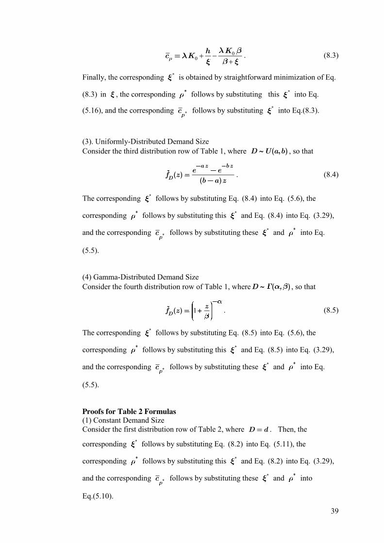
39

00 � �

�=

Khc K . (8.3)

Finally, the corresponding * is obtained by straightforward minimization of Eq.

(8.3) in , the corresponding * follows by substituting this * into Eq.

(5.16), and the corresponding follows by substituting into Eq.(8.3).

(3). Uniformly-Distributed Demand Size Consider the third distribution row of Table 1, where ( , )D U a ba , so that

( )( )D

az bze e

f zb a z

. (8.4)

The corresponding * follows by substituting Eq. (8.4) into Eq. (5.6), the

corresponding * follows by substituting this * and Eq. (8.4) into Eq. (3.29),

and the corresponding follows by substituting these and into Eq.

(5.5).

(4) Gamma-Distributed Demand Size Consider the fourth distribution row of Table 1, where ( )D ,a , so that

1( )D

zf z � . (8.5)

The corresponding * follows by substituting Eq. (8.5) into Eq. (5.6), the

corresponding * follows by substituting this * and Eq. (8.5) into Eq. (3.29),

and the corresponding follows by substituting these and into Eq.

(5.5).

Proofs for Table 2 Formulas (1) Constant Demand Size Consider the first distribution row of Table 2, where =D d . Then, the

corresponding * follows by substituting Eq. (8.2) into Eq. (5.11), the

corresponding * follows by substituting this * and Eq. (8.2) into Eq. (3.29),

and the corresponding follows by substituting these and into

Eq.(5.10).

*c*

*c* *

*c* *

*c* *

40

(2) Exponentially-Distributed Demand Size Consider the second distribution row of Table 2, where Exp( )D a .

Substituting Eq. (5.14) into Eq. (5.9) yields,

11� �

�=

D

Khc K . (8.6)

Finally, the corresponding * is obtained by straightforward minimization of Eq.

(8.6), the corresponding * follows by substituting this * into Eq. (5.16), and

the corresponding follows by substituting this into Eq. (8.6).

(3) Uniformly-Distributed Demand Size Consider the third distribution row of Table 2, where ( , )D U a ba . Then, the

corresponding * follows by substituting Eq. (8.4) into Eq. (5.11), the

corresponding * follows by substituting this * and Eq. (8.4) into Eq. (3.29),

and the corresponding follows by substituting these and into Eq.

(5.10).

(4) Gamma-Distributed Demand Size Consider the fourth distribution row of Table 2, where ( )D ,a . Then, the

corresponding * follows by substituting Eq. (8.5) into Eq. (5.11), the

corresponding * follows by substituting this * and Eq. (8.5) into Eq. (3.29),

and the corresponding follows by substituting these and into Eq.

(5.10).

Proof for Proposition 2 Assume first that the lost-sale penalty is of the form (see

Section. 6.1). Substituting Eq. (5.16) into Eq. (5.5), we have

0� � ��

= [ ] =h

c h w , (8.7)

where the time average carrying cost is

�=

hh , (8.8)

*c*

*c* *

*c* *

001{ }xw x K( ) =

41

and the time average lost-sales penalty is

0 �= [ ]w . (8.9)

Next, equate Eqs. (8.8) and (8.9) and solve for , yielding

2

20 0 0

3 2ˆ2 2

§ ·� ¨ ¸

© ¹=

h h h . (8.10)

Letting 20

02

!h

a and 0

3 0 !h

b above, and noting that

2 2� � �a b a b , we get

2

20 0 0 0

3 2 32 2§ ·¨ ¸© ¹

h h h h . (8.11)

Eqs. (8.10) and (8.11) readily imply

03ˆ � *h , (8.12)

where the equality in Eq. (8.12) follows from the exponential case in Table 1.

This completes the proof of Eq. (5.17).

To prove Eq. (5.18), first note that h is an increasing function of by Lemma

7 (a) while w is a decreasing function of by Lemma 7(b). Second, the

aforementioned monotonicities of and in conjunction with Eq. (8.12)

imply *ˆh h and *ˆw w . Eq. (5.18) now follows from the last two

inequalities together with Eq. (5.12).

Finally, the corresponding proofs for the case 0 11 xw x Kx{ }( ) = are readily seen

to be analogous to the proofs above for 001 xw x K{ }( ) = , but with 0 replaced

by 1 . □

ˆ

h w