245

Optimal Fund Design for Investors with Holding Constraints

Remi Bourrette and Etienne Trussant

Abstract This paper examines an investor’s demand in financial products when the offer comes from a financial institution. For different reasons (costs, information), the investor does not manage his portfolio time-continuously, but instead invests in a closed-end fund. His choice results from the maximization of his expected utility, taken at the maturity date. Meanwhile, the financial institution can manage portfolios time-continuously. Given a list of assets, it thus offers all the feasible payoffs. Contrary to the usual framework, the investor only deposits part of his total wealth with the financial institution. We show that the terminal value of the balance of his wealth modifies his investment choice: the optimal payoff that we obtain can be very different from the payoff obtained when the non invested wealth is ignored. The general solution is provided by means of an implicit equation on the optimal payoff and it is illustrated by numerical examples.

Cet article traite de la demande en produits financiers d’un investisseur lorsque l’offre Cmane d’une institution financiere. Pour differentes raisons (coirts, information), celui-ci ne gere pas son portefeuille contintiment, mais investit dans un fonds ferme a horizon fixe. Son choix est guide par la maximisation de son utilite esp&!e a $ch&ce. Sa banque, elle, g&e continfiment les portefeuilles. Elle lui propose done, sur un ensemble d’actifs, tous les pay-offs rtplicables. Contrairement au cadre usuel, l’investisseur ne confie a la banque qu’un partie de sa richesse totale. On constate que la valeur a t?ch&rce de l’autre partie de sa richesse influence son choix d’investissement: le pay-off optimal peut &tre tres different de celui obtenu en ignorant la partie non investie de la richesse. La solution gCntrale est foumie par une equation donnant implicitement le pay-off optimal et est illustr6e par des exemples numeriques.

Keywords Derivative products, fund design, optimal investment, utility.

Mots clefs Conception de fonds, investissement optimal, produits derives, utilite.

Direction Recherche et Innovation, Credit Commercial de France, 103 Avenue des Champs-Elysees, F-75008 Paris (France); Tel: + 33-l-40 70 34 83, Fax: + 33-l-40 70 30 31, E-mail: dri@calvacom.fr

246

Optimal Fund Design for Investors

Having Holding Constraints

Introduction

THERE ARE TWO APPROACHES to the problem of portfolio selection. The first one,

directly derived from Markowitz’s (1952) work, addresses the allocation problem in a one period framework, with no rebalancing in between the dates of investment decision and liquidation. This method is extremely convenient for who wants to focus on specific hypotheses (e.g. the distribution of asset returns). In practice, this methodology is widely used by portfolio managers.

In the second approach, assets are reallocated on intermediary dates. It has first been explored by Samuelson (1969) and Merton (1971). Recent developments incorporate more realistic hypotheses, such as restricted short sales, constrained allocation weights or limited leverage. Grossman and Vila (1992) showed that constraints of this type alter the optimization criterion. In their paper, the constrained problem reduces to an unconstrained problem with a different risk-aversion. Among other events that may affect the investment choice, the existence of a non-financial income or the presence in the agent’s portfolio of an illiquid claim are also widely discussed in the litterature. The inclusion of wage income is a common example of this trend (see for instance the seminal papers of Samuelson (1971) an Merton (1969)) or Bodie, Merton and Samuelson (1992). Grossman and Laroque (1990) treat of illiquidity problems. They consider an agent owner of a durable good, typically a house, which generates consumption services and is illiquid because of important transaction costs. They show that transaction costs restrict trading dates and that the optimal allocation strategy is strongly dependent on the durable. Svensson and Werner (1993) address the problem of an agent holding a nontraded asset. They derive a pricing formula for this asset and highlight the importance of a so-called income hedge portfolio in the composition of the optimal allocation.

However, these approaches assume instantaneous reactions to changes in the state variables: at each date, the agent rebalances his portfolio after having solved his optimization problem. Very often, investors call on a financial intermediary to manage their portfolios. In this situation, the investment choice is made at the beginning of the period and allows dynamic strategies, as long as they are not revised during the period.

247

Leland (1980) and Brennan and Solanki (1981) have solved this problem when the investment universe is described by a single risky asset. Their results are expressed in terms of payoff profiles which are non linear functions of the risky asset terminal value. In the continuation of these studies, this paper examines the relations between a tinancial institution and a client investor. The investor makes his investment decisions on discrete time steps, since his knowledge of financial markets and his ability to trade are limited. During the interval separating two investment decisions, he deposits the amount of money he wishes to invest with the financial institution and chooses the product which suits his needs best. The products offered by the financial institution result from its capacity to trade on markets time-continuously, which allows it to build any type of derivative products. The purpose of the article is to determine what are the optimal payoff profiles, given the investor’s wealth, budget, and utility.

Section I presents a simple problem of allocation when the investor holds an illiquid claim, in a binomial framework. Section II explains the mathematical formalization of the general problem and its resolution. Section III details the situation where the portfolio separates into two terms: the hedge portfolio and the investment portfolio. Finally, Section IV gives some numerical illustrations of our results, for one and two risky assets.

I. A Simple Problem

We consider an agent who makes an investment decision over a given period. He holds an illiquid claim I’, which cannot be sold or exchanged, it will be called the non invested wealth. He also has an available budget $X to invest. His bank offers him a large line of funds, all based on a single asset 5’. More precisely, the bank offers all the payoffs Q(S) which are functions of the asset terminal value. The agent’s total wealth at the end of the period is then II’ = Q(S) + V and we assume that his objective is to maximize the expected utility of his wealth E[u( W)].

In this section we address a two binomial variables problem. The initial value of the asset S is S,, and it has two possible future values S, and S,,, S, < S, The same notations hold for V, the non invested wealth. This simplified framework aims at understanding how the two components of the agent’s wealth interact,

The joint law of the couple (S,V) under the historical probability P is described by the probabilities of each one of the four possible states. For instance, pdu denotes the probability that S = S, and V = Vu simultaneously. Our calculations also require the definition of the risk-neutral probability Q. qd then denotes the risk-neutral probability Q

248

for S = S, (resp. u). There is no need for Q to be defined on V, which, apart from being

illiquid, may also be a non financial claim. Finally, r denotes the rate of return of a risk-

free investment over the period.

The agent’s program is accordingly

mo=E[4@(S)+V)] (1)

subject to the constraint that the fimd’s price must be equal to the budget. Writing the

fund ‘s price as the expectation of its discounted terminal value under the risk-neutral

probability (I, we obtain:’

&-EQ[@(S)] = x (2)

As a function of S, the optimal profile can take two values Od = Q(S,) and QU = Q(SU).

The optimality conditions, coincide with theLagrangian derivative being equal to zero:

where R is such that the budget constraint

is satisfied.

For the sake of simplicity, we now assume that u(x) = In(x). For that type of utility,

equations (3) are second-order equations (calculations are in Appendix A). The

conclusions that we draw are a good illustration of the main effects induced by our

approach. Those effects clearly are highlighted in the following numerical results.

1 In this binomial framework, all the profiles are the payoffs of buy-and-hold strategies. The fund’s price is then directly related to the proportion of S in the portfolio.

249

-1.0 -0 8 -0 6 -0 4 -0.2 0 0 02 04 06 08 1.0

Correlation

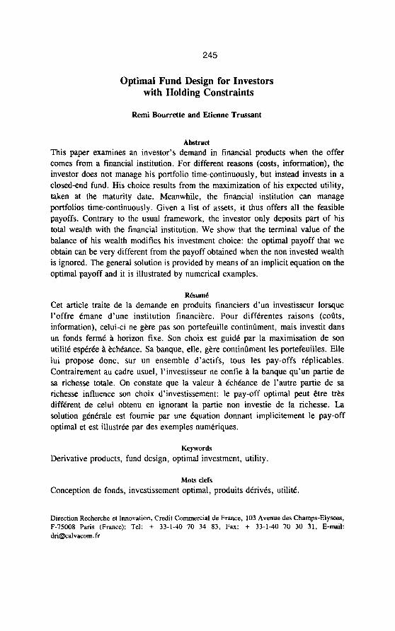
X= $20, So = $100, S, = $90, S, = $125. V‘, = $80, v,, = $140 r=5%,P(S=S,)=P(V=6’,)=0.5.

Figure 1. Values of Qd and ‘3” as functions of correlation. The plots show the values of the

optimal payoff function when the asset takes its lower value (filled dmnonds) and its upper value (open

squares).

Figure 1 shows the plot of the two values md and QU of the optimal profile for various values of the correlation between S and V. For a correlation greater than a critical value p0 2 0.6, the optimal profile is inverted: it pays more when S is low than when S is high. When the correlation is under the critical threshold, the profile payoff increases with the asset. For low values of the correlation, the agent even borrows to buy more of the asset. That generates a leverage effect which increases as the correlation decreases. At the critical value p,,, the optimal investment is the riskless asset. Figure 2 shows the value of the investor’s indirect utilityz, when the correlation is again the varying parameter. The function reaches its maximum when the two random variables are perfectly anticorrelated. It reaches its minimum at the critical value of inversion, which corresponds to a riskless optimal investment (proof in Appendix B).

2 The indirect utility is 17 = .@[u(@(S) +V)].

250

-1.0 -0 8 -0 6 -0.4 -0.2 0.0 0.2 0.4 0.6 0.8 1.0

Figure 2. Indirect utility as a function of correlation.

The inverted profile appearing for high enough values of the correlation is an unusual result. The agent’s behavior is justified in that the risk he is bearing with V is too great for his risk aversion, whatever his expected total wealth. Therefore, selling the risk generated by Vwill decrease his exposure. When V is positively correlated with the asset, the best decision is to be short on the asset, hence the inverted profile. When it is anticorrelated, the agent takes advantage of the leverage effect, which makes the financial wealth more volatile than the asset but once again lowers his total risk.

The profile’s asymmetry, i.e.: the fact that, for a null correlation, the optimal solution is positively indexed on the asset, comes from the positivity of the asset’s risk premium. Risk diminution is not the only objective of our program, high expected returns are also a source of utility. In the present example, the low amount of invested wealth ($20) with regard to the illiquid claim ($80 or $140 at the end of the period), makes the first effect stand out. However, when the illiquid wealth becomes negligible compared to the budget, the solution naturally tends to the classical one, in which the whole wealth is invested. Finally, the indirect utility is maximum for a perfect anticorrelation, because the agent takes advantage of selling the risk of V and of purchasing the asset risk premium simultaneously.

251

An incomplete analysis would lead a risk-averse investor to avoid seemingly risky behaviors. That in turn may prevent him from achieving optimality. Investment must not be analyzed independently of the agent’s other concerns. We will now formalize this key idea.

II. Model and General Resolution

A. Hypotheses

Our framework is monoperiodical because of one basic consideration: time continuous portfolio management is not cost-free for the agent. The bill is paid both in transaction costs and in leisure time spent in gaining information about financial news, not to speak of the market accessibility for small private investors, The investment opportunities available to the agent are then more likely close to the lines of mutual funds offered by financial institutions than to the set of all the payoffs feasible by duplication techniques. A billing argument based on management costs would hold for financial institutions if they wished to offer a tailored product to each one of their clients. However, such is usually not the case and sophisticated products can then be offered to private investors as long as they are not overly customized. A natural limitation, already in use, is to fix the possible dates for subscription and buyback. In our search of optimality, we will accordingly be interested in any profiles of payoff functions at a given future date rather than in products that generates intermediary cash-flows. This leads to the following assumption:

A~SLMPTION 1: The agent does not manage his portfolio time continuously. His opportunities of investment are resticted to the products offered by the financial institution. For all these products, the payoff occurs at date T.

Under Assumption 1, the agent’s program can be seen as a two-step optimization, The first decision the agent has to make is the choice of his consumption plan between the period. One part of this decision is the amount X of his initial wealth to be invested in financial products maturing at T. Secondly, given this initial decision, the agent solves a classical intertemporal program, which includes a change in wealth at T resulting of the initial investment. We will focus on the investment decision. The term “investment”

252

refers to a positive budget X, but the approach is the same when X is negative, i.e.: when the agent has to borrow.

Assumption 2 states the agent’s preferences.

ASNhfFTION 2: The agent’s utility at date Tis a function of his total wealth at this date, u( W, ). This function is increasing, strictly concave and twice continuously differentiable.

According to this framework, the optimal investment problem consists in maximizing the expectation EP[~(~T)], k ta en in t = 0, under the agent’s probability, being given X, More precisely, we aim to identify the optimal payoff in T for an initial investment of $X in t = 0. Note that the discrete time approach can capture discontinuities in the consumption rate more easily than a time continuous approach. In particular, the purchase of durable consumption goods, such as a real estate operation, is well described by our framework.

The total wealth must be modeled with care. It consists of two parts. The first one is invested in financial products. Folowing Assumption 1, it is available at the end of the period. We will call it the agent’s invested wealth. The second one is what the agent wants to keep liquid or, on the contrary, the present value of the illiquid claims he holds or he will be led to hold before T, and that therefore cannot be invested. We will call the second part of the agent’s wealth the non invested wealth. Let’s review a few examples. For an individual whose only patrimony is his human capital, the non invested wealth is the sum of the liquidity he holds and of his discounted future earnings. The non invested wealth, which can be negative, may also be a real estate claim, bought or sold by the agent.

A classical rule in portfolio selection consists in maximizing the utility of invested wealth only. We will show that non invested wealth strongly influences the investment decision, even when it has no equivalent on the financial markets.

The wealth W, in T has two components: the payoff 0, of the financial product and the non invested wealth, described by a random variable denoted by Vr

The agent’s wealth at T represents his total patrimony at this date. The agent is bankrupt as soon as his wealth is negative. To avoid the occurence of such events we assume:

253

AS~LMPTION 3: The total wealth at T must be positive.3

This assumption has some consequences on QT since W, = Qr +V, must be positive.4

Let V,,,(s) be the minimum of all the possible values of V, conditionnally on S = s:

V,,(s) = max(v;P(V 2 vlS = S) = 1).

We assume that this number is always finite. Then, Q(s) t -Vm,, (s) must be true for all s,

to insure the (almost-sure) positivity of the total wealth.5

The financial product is issued by a financial institution such as a bank, an insurance

company or a fi,md. In order to define the kind of product the institution is able to offer,

the usual assumption is stated:

ASSUMPTION 4: For the financial institution, the markets are perfect and arbitrage,free.

For a given list of assets chosen among all those the financial institution can trade, the

institution is then able to propose any payoff of the following form:

where S, is the vector of the asset prices in T, and the profile @ is a real fimction. Under

Assumption 4, all the profiles are feasible by the financial institution. Our purpose is to

determine the agent’s optimal demand for the profiles.

For the institution, at the beginning of the period, the cost D0 of the profile QT is

given by a risk neutral valuation:

Do = Ee[Z,-‘@(S,)]

3 In the mathematical development that follows, the total wealth can be zero. However, the results are unchanged even if the utility function is not defined in zero, as scan as the total wealth is almost surely strictly positive.

4 In the binomial example of section II, the positivity constraint was not binding.

5 If Dr is the result of an investment in a fund, its positivity is also required. This case will not be detailed, but its resolution can easily be deduced from the general program by replacing -V,,,, by max(O,-I&).

254

where Q is the risk-neutral probability, whose existence is ensured by assumption 4, and Z, is the accounting factor over the period [0, T]. If r, is the instantaneous continuously compounded risk-free interest rate,

Z, is the payoff of a monetary investment, thus, it may be included in the list of assets

B. The Mathematical Problem

Under the above assumptions, the agent’s program is a functionnal optimization on the profile, under the budget constraint. The criterion is the expected utility at T, which is a function of the agent’s wealth at this time:

subject to the budget constraint:

EQ[Z-‘a@)] = x

(10)

(11)

and subject to the wealth positivity constraint:

Q(s) 2 -V,,” (s) , for all s, (12)

where all the time subscripts are omitted for simplicity. For the above program to admit a solution, it is necessary that the constraints do not define an empty set of profiles, i.e.: the budget must be high enough to insure the agent against bankruptcy:

x 2 -EQ[z-‘vm,.(S)j = xm, (13)

In the following, we will call admissible budget a budget that verifies this inequality. We will note g(s) the density of S under the agent’s probability P and h(s) the density of S under the risk-neutral probability Q. Defining II(s) by

1 go ‘(‘)= Ee[Z-‘IS=s] h(s)’

(14)

we obtain (proof in Appendix C):

THEOREM 1: Assuming u’(+co) = 0, there is one and only one solution to the agent’s program for admissible budgets. This solution fulfills

E’[d (Q(s)+ V)lS= s] = &

if Q(s) > -V,,,(s), and Q(s) = -V,,,(s) otherwise, 1 being determined through the budget constraint.

This equation is a generalization of equation (2) of Leland (1980) or, equivalently, of equation (3) of Brennan and Solanki (1981). The first two additionnal elements are the randomness of the interest rate and the vectorial form of S. But the main difference is the introduction of the non invested wealth.

Marginal utility

In the particular case V = 0, the interpretation of equation (15) is classical, h(s)Ee[Zm’IS = s]ds can be seen as an Arrow-Debreu price, corresponding to the state of the world S E[S,S +ds]. This equality is an optimality relation on marginal utilities, holding for every states of the world. In the most general case for V, the interpretation is unchanged, nevertheless, the marginal utility takes V and its possible interdependence on S into account.

Preferences and beliefs

Equation (15) links the two main inputs of our problem, i.e. the utility function u and the agent’s distribution g, to the output @. This triple sided relation can be used in different ways, either to indent@ the preferences (u) or the beliefs (g> of the agent, Leland (1980) for instance, determines the implicit preferences of an agent investing in insurance products, characterized by convex profiles.

256

Risk-neutral valuation and numeraire portfolio

The f%nction n(s) is defined by (14) at the end of the period. We can similarly define

a fimction n,(s), at every instant t, with the probability distributions of S, and Z, .6

n,(S,) is then the numeraire attached to the historical probability. It is the numeraire

portfolio defined by Long (1990). Expressed in II,(J) units, all the self-financing

strategies based on the set S of assets are martingales: if U, is the value at t of a self-

financing strategy, and since II, (S, ) = 1, we have

EP [ 1 & = EQ[~EQ(Z;‘~S,)]=EQ[~Z~~‘]=-& (16) 0 0

Furthermore, the risk-neutral valuation is not the only possible, any choice of numeraire

instead of the accounting factor would give the same results and also the same numeraire

portfolio.

Indirect utility

Let U(X) be the indirect utility of the budget X. U(X) is the expected utility of the

optimal profile:

U(X) = EP[u(Q(S)+6’)], (17)

and we have U’(X) = 1. It has been shown in the proof of Theorem 1 that [J’(X) is

decreasing. It also tends toward A,,,,, when X tends toward the lower bound of the

admissible budgets and toward 0 when X tends toward +oo.

The set of profiles

We have already mentionned that the set of the optimal profiles is ordered. In

particular, all the profiles are distinct and do not cross over. The lower profile is -ri,,,

and corresponds to the lower admissible budget X,,,

6 II,(s)= where Z, is the accounting factor in f, S, the vector of the asset

prices in t, g, (resp. h,) the density of S, under P (rap. Q).

257

III. The Separable Case

As it has been said in Section III, two elements jointly determines the agent’s program. his non invested wealth and his utility function. They typically cannot be dissociated. In this section, we focus on a situation which allows the dissociation. It makes the interpretation of Theorem 1 clearer.

A. Decomposing Into Expectation Terms

Let Y(S) denote the expectation of V, conditionnally on S:

Y(S) = EP[V(S = s], for all s. (18)

We have

V-Y(S)+& and EP(e)=O (19)

The decomposition of I’ into a function of S and a residual E is unique, it aims at separating the part of the fluctuations in V which are “directly” explained by S from those that are not. The linearity of the relation does not preclude from non linear dependencies of the residual in S. However, the residual is sometimes independent from the vector of assets. When it is the case, the optimality equation becomes

Note that the lower bound of all the residual possible values is constant as a result of its independence on 5’:

max(v; P(V 2 vlS = s) = l] = Y(s) + max(e; P(E 2 elS = s) = 13, (21)

and then

V,,“(s) = Y(s)+max(e;P(~> e) = 1) = Y(s)+ E~~“. (22)

Let’s now define a new utility function uC , defined on [ --E,,~, +co[, as

u,(w) = EP[u(w + e)]. (23)

258

It is twice continuously differentiable, increasing, concave and also satisfies uE’ (+03) = 0, The hnction y, = 0 + Y which appears in the optimality equation complies with the

modified constraints of budget

P[z-‘q(S)] = x+P[z-‘w(s)], (24)

and positivity

PCs) 2 - %,“~ (25)

THEOREM 2: If S and its residual care independent, the optimal profile is

O(s) = UE’ -’ a ( 1 - -Y(s) n(s)

if l/n(s) < u’ c (- E,,,,, ) , and Q(s) = - E,,,,, - ‘-I-‘(s) otherwise, R being determined through

the budget constraint and uE being defined by equation (23).

Following the above remarks, the proof of Theorem 2 is nothing but a change in the notations, the conditions for existence and uniqueness of the solution being those of the original problem. The new optimization program is separated in two parts. The first one consists in a cancellation of the effects of V that can be captured by the investment (-Y), Because the agent is risk-averse, he will try to suppress the randomness of the part of his wealth he cannot control. Using the money he has left, possibly negative, he solves a utility program differing from its original version by his preferences (for the changes in utility caused by holding constraints, see Grossman and Vila (1992)).

The utility f%nction is consequently not an absolute criterion. The criterion to be maximized directly depends on the accuracy of the description of the agent’s wealth. For instance, when the original utility finction is CARA, the new utility fimction remains CARA with the same absolute risk aversion7; however, for a given budget, and though the preferences are the same, the optimal profile in the presence of non invested wealth is different from the profile obtained with V = 0. In fact, the effects of non invested wealth appear through the translation of Y.

7 For a Constant Absolute Risk Aversion utility u(x) = -e-“/y, therefore, 11, = ku with k = /?[exp(-p)].

259

The positivity constraint on total wealth is also important since it introduces a lower bound, typically depending on S, on the profiles. In some situations, the optimal profile may present a constant, positive lower bound, and is then a guaranteed fund. The most direct example of such guaranteed profiles is obtained with a constant negative non invested wealth, a debt, for instance : if V = -p’, the optimal profile Uills Q(s) 2 v > 0. In the absence of debt, there is no particular reason for the guaranteed funds to be optimal, as is illustrated in the next part.

B. Zero Non Invested Wealth

We focus on the case where all the wealth is invested, or, in other terms, the non invested wealth V is zero. This approach is classical. Nevertheless, on one hand, in the asset allocation problems derived from Markowitz’s theory, the terminal payoffs are restricted to linear profiles on several assets (buy-an-hold strategies). On the other hand, the profiles proposed by Leland (1980) and Brennan and Solanki (198 l), are written on a single asset. Our purpose is to derive some more general properties from Theorem 1, in a simplified framework.

When the wealth is entirely invested (V = 0), the optimal profile is, for every value of the vectors,

a Q(s) = ZP - ( 1 w4

(27)

if A/II(s) <u’(O), and a(s) = 0 otherwise, ;1 being determined through the budget constraint. This result is an application of Theorem 2, with V = V,,, = 0 and then &mln = 0 and ‘I-‘=O.

C. Zero Non Invested Wealth and Log-normal Asset Prices

We now assume that the short term interest rate r is constant and that the evolution of the risky asset prices is governed by

dSx/S, = (r +p,)dt+gdBi (28)

where p, is the constant risk premium and o, the constant volatility of asset i, and B, is a n-dimensional Wiener process under the historical probability P. Let C be the variance-

260

covariance matrix of the instantaneous rates of return of the assets per unit of time.8 Girsanov’s theorem explicits the unique equivalent risk-neutral probability Q under which:

dS,/S, =rdt+qdBh (29)

where Be is a Q-Wiener process with the same variance-covariance matrix. We have for all s=(s,,s2 ,..., s,),

H(s) = ksp’$‘, ,S,““, (30)

with

a = C-‘p (31)

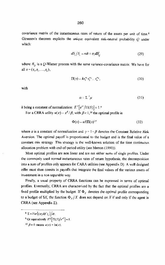
k being a constant of normalization: EP[e’r/II(S)] = 1.9 For a CRRA utility u(x) = xBlp, with pi l,i” the optimal profile is

O(s) = am(s)“7 (32)

where a is a constant of normalization and y = 1 -p denotes the Constant Relative Risk Aversion, The optimal payoff is proportionnal to the budget and is the final value of a constant mix strategy. This strategy is the well-known solution of the time continuous allocation problem with end-of-period utility (see Merton (1990)).

Most optimal profiles are non linear and are not either sums of single profiles. Under the commonly used normal instantaneous rates of return hypothesis, the decomposition into a sum of profiles only appears for CARA utilities (see Appendix D). A well designed offer must then consits in payoffs that integrate the final values of the various assets of investment in a non separable way.

Finally, a usual property of CRRA functions can be expressed in terms of optimal

profiles. Eventually, CRRA are characterized by the fact that the optimal profiles are a fixed profile multiplied by the budget, If ax denotes the optimal profile corresponding

to a budget of $X, the function a, / X does not depend on X if and only if the agent is CRRA (see Appendix E)

8 x =Va’((a#f),)/dt. g Or equivalently Ee[ 17(S)/er’] = 1.

lo ,f3= 0 means u(x) = In(x).

261

IV. Numerical Examples

A. A Single Asset Problem

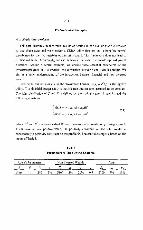
This part illustrates the theoretical results of Section II We assume that S is reduced

to one single asset and we consider a CRRA utility function and a joint log-normal

distribution for the two variables of interest V and S. This framework does not lead to

explicit solutions. Accordingly, we use numerical methods to compute optimal payoff

functions. Around a central example, we decline three essential parameters of the

investor’s program: his risk aversion, the correlation between S and c’and his budget, We

aim at a better understanding of the interaction between financial and non invested

wealth.

Let’s detail our notations. T is the investment horizon, u(x) = xpI/? is the agent’s

utility, X is his initial budget and r is the risk-free interest rate, assumed to be constant.

The joint distribution of S and V is defined by their initial values SO and VO and the

following equations:

dS/S = (Y + pu,)dt + usdBs (33)

dV/V = (r + pv )dt + q,dB”

where BS and B” are two standard Wiener processes with correlation p, Being given S,

V can take all real positive value; the positivity constraint on the total wealth is

consequently a positivity constraint on the profile 0. The central example is based on the

inputs of Table I.

Table I

Parameters of The Central Example

Agent’s Parameters Non Invested Wealth Asset

T p X r V, p,, o, p SO ,u~ O,

5 yrs -1 $10 5% $100 3% 20% 0.7 $100 3% 15%

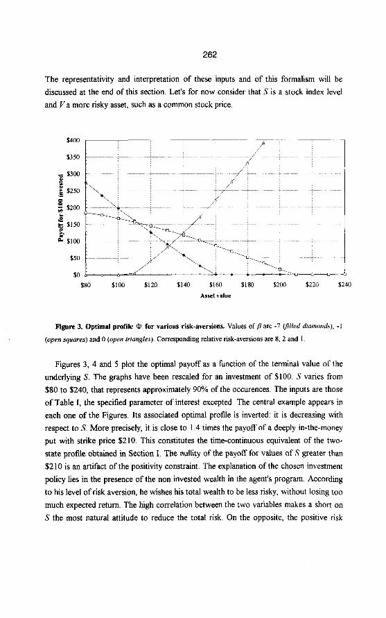
The representativity and interpretation of these inputs and of this formalism will be discussed at the end of this section. Let’s for now consider that S is a stock index level and V a more risky asset, such as a common stock price.

$350

F $300

3 & $250 .m 8 z $200

3 k $150

k $100

$50

$0

$80 $100 $120 $140 $160 $180 $200 $220 $240

Asset value

Figure 3. Optimal profile Q for various risk-aversions. Values of p are -7 v/led diamonds), -1

(open squares) and 0 (open triangles). Corresponding relative risk-aversions are 8, 2 and 1.

Figures 3, 4 and 5 plot the optimal payoff as a function of the terminal value of the underlying S. The graphs have been resealed for an investment of $100. S varies from $80 to $240, that represents approximately 90% of the occurences. The inputs are those of Table I, the specified parameter of interest excepted. The central example appears in each one of the Figures. Its associated optimal profile is inverted: it is decreasing with respect to S. More precisely, it is close to 1.4 times the payoff of a deeply in-the-money put with strike price $210. This constitutes the time-continuous equivalent of the two- state profile obtained in Section I. The nullity of the payoff for values of S greater than $210 is an artifact of the positivity constraint, The explanation of the chosen investment policy lies in the presence of the non invested wealth in the agent’s program. According to his level of risk aversion, he wishes his total wealth to be less risky, without losing too much expected return. The high correlation between the two variables makes a short on 5’ the most natural attitude to reduce the total risk. On the opposite, the positive risk

263

premium of S motivates for a long rather than a short position. One effect dominates the other according to the importance granted to the total risk. Finally, diversification also reduces the influence of the specific risk of V.

Figure 3 presents various profiles obtained for differently risk-averse investors. The inversion effect increases with the risk-aversion, On one hand, for a risk aversion of 8, the slope of the payoff is deeper than in the central example. On the other hand, for a risk aversion of 1, the investment is positively indexed on S. The agent tries to benefit from the risk premium of the asset and even allows his total wealth to be riskier than his non invested wealth. As in the binomial example, in all of the three cases, the investment is levered, (i.e.: the slope is greater than one).

‘CI 2 0 $200 t .- 8 fi $150

2 b p. $100

k

$50

3 x

$80 $100 $120 $140 $160 $180 $200 $220 $240

Asset value

Figure 4. Optimal profile Q, for various budgets. Values of budget X are $5 (filled diamonds), $10

(open squares), $20 (open frrangfes) and $50 (crosses). The last line (stars) corresponds to an infinite

budget, or equivalently to a zero non -invested wealth.

For a given investor, the risk-aversion is fixed, in this example, it is worth 2. Among the parameters that may change the investor’s policy is of course his budget, For some values of the budget, Figure 4 plots the optimal profiles. The smaller the budget, the deeper the inversion of the profile, since only the total wealth and the implied risk matter. An agent with a very low budget is ready to lose it all if it insures him against a large fall

264

in the value of his non invested wealth. This insurance goes through the 0.7 correlation

between S and V: for a budget of $5, if S loses 20% over 5 years, V is likely to be low,

and the agent’s receives twice and a half his budget, $12.5 dollars (or $250 for $100

invested). For high budgets, the problem tends to the problem of Section III Part B,

where all the wealth is invested. The principle which rules the agent’s strategy is then

investment, while it was insurance for small budgets.

The slope of the profile is not important in itself, it is the joint behavior of S and V

that is preponderant in the profile’s design, as shown in Figure 5. In the central example,

the agent aims at enforcing an insurance strategy. He tries to get a high return on his

investment when his non invested wealth is low. Accordingly, when the correlation is

negative, the profile is positively indexed on S, when it is positive, it is negatively

indexed. At correlation zero, insurance is impossible, the asset’s risk premium justifies

the call-type investment

$350

$50

$0 -4 $80 $100 $120 $140 $160 $180 $200 $220 $240

Asset value

Figure 5. Optimal profile Q for various correlations. Values of correlation p are 0.9 (filled

diamonds), 0.7 (open squares), 0 (open fmngles) and -0.5 (crosses). Indirect utilities (multiplied by

100) arc respectively: -0.807, -0.828, -0.938 and -0.953.

The well-known joint-lognormal distribution is rich enough to describe many

situations. S can always be considered an index level, on a market whose choice depends

265

on the non invested wealth. In our example, the indiret utility increases with the

correlation, the best index would hence be the most correlated to the non invested

wealth. Let’s now review two examples.

Dwelling is a typical example of an illiquid claim held by households. I’ could then

represent the price of a house at a preset selling date, and S could be a real estate-based

asset. The expected level of correlation between S and the house price is positive. Most

often, the budget devoted to financial operations will be small in comparison to the value

of the dwelling. A useful1 product that could be proposed by the banks is hence a

reverse-index fund, insuring investors against real estate kruchs. Strongly risk-averse

clients would be the natural subscribers of such a product.

Holding large amounts of money in the form of stocks of a single firm is also a

common situation. Executives often receive stocks of their company, or, equivalently,

deeply in-the-money stock options, as a complement to salary, such that stocks may

become the main component of their wealth. The obligation to keep them implies a risk

exposure. A possible way of diminishing the exposure is to buy a reverse-stock index

fund. However, the choice of inverted profiles is far from being systematic, as it is

obviously shown by Figures 3, 4 and 5.

B. A Two Assets Problem

We now apply our results to optimal profiles on two assets. We keep the same

hypotheses than in Part A, but we introduce a second asset S,. It is jointly log-normal

with the non invested wealth and the first asset (previously denoted by S, now by S,). Its

charasteristics are mentionned in Table II. This additional asset can be seen as a long

term bond index, the first asset being a stock index. We assume that the discounting term

of equation (19) does not depend on any of the two assets, its conditionnal expectation is

then constant. The non invested wealth, positively correlated with the stock index, is

independent from the long term interest rates. When the agent holds a claim whose

behavior is close to the stock index and has subscribed a long-term credit, such a

characteristic could be observed, because the negative correlation of the two

components of the agent’s wealth may cancel the influence of the long term interest rates.

Table II

Additional Parameters

Asset 2 Correlations

P2 0, 42 Pv2

1% 5% 0.3 0

Figure 6 presents, with the same convention than in Part A, the optimal profile on the assets S, and .S, for an agent whose wealth is entirely invested, with initial value $10. The solution, given in Section III Part B, is explicit:

This profile is well approximated by a buy-and-hold strategy, in the proportions of Markowitz’s portfolio. These proportions are: 5 1% stocks, 153% bonds and -104% risk- free asset.

Figure 6. Optimal profile @(s, ,s2) without non invested wealth.

267

The solution of the actual program is plotted on Figure 7. The correlation of V with the stock index, as in the single asset case, leads to inverted payoffs. On the contrary, the zero correlation with the bond index implies a positive exposure to the bond market, in order to capture the risk premium.

Figure 7. Optimal protile O(sI ,s2) in presence of non invested wealth.

V. Conclusion

The focus of our paper is on optimal fund design for an investor who delegates his porfolio management to a financial institution. We have assumed that the investor chooses the fund in which to invest at the beginning of the period, according to his preferences and to his non-invested wealth, i.e.: the part of his wealth which is not deposited with the financial institution. The role of the institution is then to duplicate the payoff profile chosen by the investor. Under general assumptions on the distributions of asset prices, we have derived an implicit equation on the optimal profile. We have shown that the optimal investment combines hedging against unfavorable values of the non- invested wealth and pure investment logic. When the hedging effect predominates and when the non-invested wealth is positively correlated with the asset returns, optimal profiles are decreasing functions of asset prices. This has been presented in our numerical examples. The demand in investment products is thus strongly related to the part of the

268

investor’s wealth that is not deposited with the financial institution. Also note that a limited set of payoff profiles, together with the basic assets, can suffice to build buy-and- hold portfolios that are good proxies of optimal profiles. What more, though our examples are oriented towards fund management, methodologies and conclusions are the same for credit demand. Finally, further developments may consider a more general form of utility (e.g.: u(@, V) instead of u(@+ V)) or the investor’s utility in case of early buyback.

Appendix

A. Resolution of System (3). When U(X) = In(x) , system (3) becomes

where the risk-neutral probability Q is classically given by

% = S” -(l+r)S,

su - Sd

(AlI

WV

and q, = I-q,

Multiplying the first equation of system (Al) by (Q), +V,)(md +VU) leads to a second order polynomial equation in Qd, that is easily solved. The same method applies to Q’,,. Finally, equation (4) yields 1.

B. Comments On The Critical Threshold pO. Denoting by E,, B(p) and U(p) respectively the expectation operator under P, the optimal payoff and the indirect utility when correlation is p, we have

269

the penultimate equality coming from the fact that the law of Q(p,) + b’ does not depend

on A precisely because @(p,,) = (1 + r)X is deterministic.

C. Proof of Theorem 1. In the following, we will call admissible budget a budget that

verities this inequality. We will note g(s,v) the density of the couple (S,k’) under the

agent’s probability P, and h(.s,z) the density of the couple (S,Z) under the risk-neutral

probability Q. The problem’s Lagrangian is then

where A. is a real number and p(s) is a real mnction of s. The Lagrangian’s differential in

CD, is, for any function Y:

&&) = ISY(.~)rr’(~(.~)+,~)~(~,l’)d~d”

-Aj++)h(s,z)dsdz -jp(s)Y(s)ds z

(A5)

Defining J5, for y 2 -I’,,,,, (s) by

Jl(Y) = r;;:,, d(y + v)g(s, v)dv, (‘46)

the optimality equation ~55, = 0 leads to the condition to be satisfied by the optimal @, if

it exists:

when Q(s) z -I’,,,,,(s),

,u(s) = 0 or equivalently Js(@(s)) = ljlh(z,s)dz, z

6474

when Q(s) = -V,,,,(s), (A7b)

p(s) 2 0 or equivalently J$(@(s)) I l~~h(r,s)dz. Z

Being given 1, for every value of s, we thus have to find a real number y = Q(s)

satisfying the above system. Since U’ is strictly decreasing and continuous, .7$(y) is a

strictly decreasing function of y. Moreover, II’ admits a limit in +co and we assume

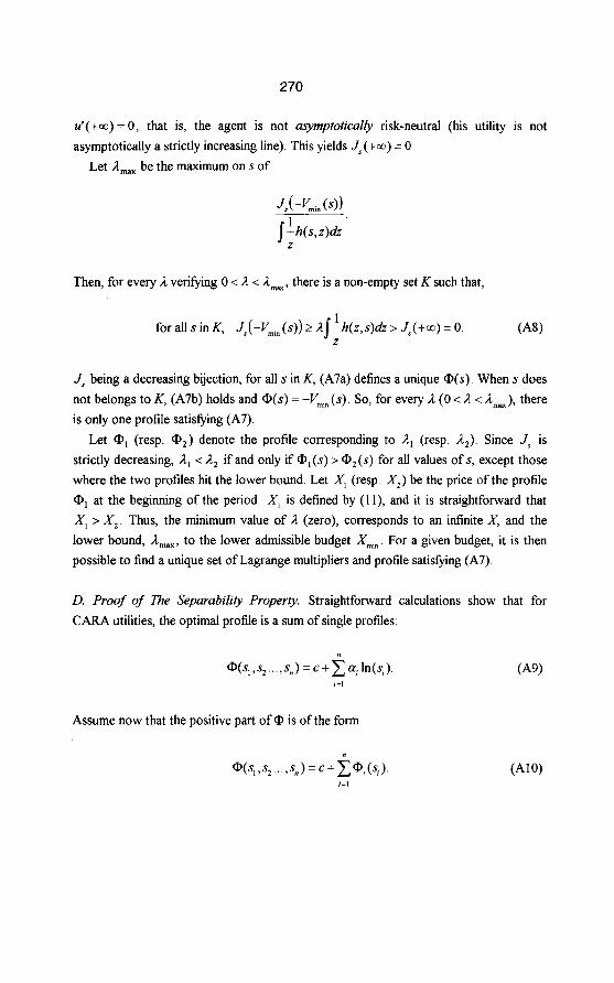
270

u’(+co) = 0, that is, the agent is not asymptotically risk-neutral (his utility is not asymptotically a strictly increasing line). This yields J$(+clo) = 0.

Let Lax be the maximum on s of

J,(-v,,, (4) I L(s,z)&

Z

Then, for every R verifying 0 < I < A,,,=, there is a non-empty set K such that,

for all s in K, J,(-V,,,(s)) t l~~h(z,s)& > J$(+m) = 0. (‘48) Z

J, being a decreasing bijection, for all s in K, (A7a) defines a unique Q(s). When s does not belongs to K, (A7b) holds and D(s) = -V,,(s). So, for every R (0 < ;1< &,,,), there is only one profile satisfying (A7).

Let 0, (resp. m2) denote the profile corresponding to il, (resp. I,). Since J2 is strictly decreasing, II, < il, if and only if Q,(s) > Q2(s) for all values of s, except those where the two profiles hit the lower bound. Let X, (resp. X,) be the price of the profile @r at the beginning of the period. X, is defined by (1 l), and it is straightforward that X, > X,. Thus, the minimum value of il (zero), corresponds to an intinite X, and the lower bound, I,, to the lower admissible budget Xmln. For a given budget, it is then possible to find a unique set of Lagrange multipliers and profile satisfying (A7).

D. Proof of 7lhe Separability Property. Straightforward calculations show that for CARA utilities, the optimal profile is a sum of single profiles:

Assume now that the positive part of Q, is of the form

@(s,,s2 . ..) s”)=c+cq(s,). ,=,

271

The logarithmic partial derivative of the ratio of densities with respect to the i-th component is derived from equation (30) :

dn(h’g) = --(r /s a, ”

Using the equation of optimality and (Al 0) yields

-t!&)) =-E!-- u’ s,@ I 6, >

(All)

6412)

As a function of each separated component s, , the absolute risk aversion is constant

E. Proof of Budget Invariance. Let @ be the optimal profile for a fixed budget, say X = 1. If the problem is budget-invariant, then, for all X and s, we have

u’(Xaqs)) = n(x)@) W3)

and for all X, y

u’(G) = 4WF(Y), 6414)

where F(y) = (h/g) 0W. It is a classical result that if A(xy) = B(x)C(y) for all x, y then A is a power function.

REFERENCES

Benninga, S., and M. Blume, 1985, On the optimality of portfolio insurance, Journal of Finance 40, 1341-1352.

Bajeux-Besnainou, I., and R. Portait, 1995, Pricing contingent claims in incomplete markets using the numeraire portfolio, AFFI Conference, June 29.

Black, F., and M. Scholes, 1973, The pricing of options and corporate liabilities, Journal of Political Economy 8 1, 63 l-654.

272

Bodie, Z., R. C. Merton, and W. F. Samuelson, 1992, Labor flexibility and portfolio

choice in a life-cycle model, National Bureau of Economic Research, working paper

No. 3954.

Breeden, D. T. and R. H. Litzenberg, 1978, Prices of state contingent claims implicit in

options prices, Journal of Business 5 1, 62 l-652.

Brennan, M. J., and R. Solanki, 198 1, Optimal portfolio insurance, Journal of Financial and Quantitative Analysis 16 3, 279-300.

Cox, C., and C. Huang, 1989, Optimal consumption and portfolio policies when assets

prices follow a diffusion process, Journal of Economic Theory 49, 33-83. Cox, C., and C. Huang, 1991, A variational problem arising in financial economics,

Journal of Mathematical Economics 20, 465-87. Friend, I., and M. E. Blume (1975), The demand for risky assets, American Economic

Review, 64, 900-92 1.

Grossman, S. J., and G. Laroque, 1990, Asset pricing and optimal portfolio choice in the

presence of illiquid consumption goods, Econometrica 58, 25-52. Grossman, S. J., and J.-L. Vila, 1992, Optimal dynamic trading with leverage constraint,

Journal of Financial and Quantitative Analysis 27 2, 15 1- 168.

Harrison, J. M., and S. Pliska, 1981, Martingales and the stochastic integrals in the

theory of continuous trading, Stochastic processes and their applications, 11.

Lease, R. C., W. G. Lewellen, and G. G. Schlarbaum, 1974, The individual investor:

attributes and attitudes, Journal ofFinance 29, 413-438.

Leland, H. E., 1980, Who should by portfolio insurance ?, Journal of Finance 35 2, 58 l-

94.

Lioui, A., and P. Poncet, 1994, Optimal hedging in a dynamic futures market with a

nonnegativity constraint on wealth, CEREXSEC, working paper No. DR 95005.

Long, J. B., 1990, The numeraire portfolio, Journal of Financial Economics 26, 29-69 Markowitz, H., 1952, Portfolio Selection, Journal of Finance, 7. Merton, R. C., 1971, Optimum consumption and portfolio rules in a continuous time

model, Journal of Economic Theory 3, 373-4 13.

Morin, R.-A., and F. Suarez., 1983, Risk Aversion Revisited, Journal of Finance 38 4, 1201-1216.

Projector, D. S., and G. S. Weiss, 1966, Survey of financial characteristics of consumers,

U.S. Federal Reserve Technical Papers, Board of Governors of the Federal reserve

System, Washington D.C.

Samuelson, P. A., 1969, Lifetime portfolio selection by dynamic stochastic

programming, Review of Economics and Statistics 5 1, 239-246.

Svensson, L. E O., and I M. Werner, 1993, Nontraded assets in incomplete markets.

Pricing and portfolio choice, Europenn Economic Review 37, 1149-68.