optimal dynamic strategies for index tracking and
TRANSCRIPT

Optimal Dynamic Strategies for IndexTracking and Algorithmic Trading
Brian Ward
Submitted in partial fulfillment of the
requirements for the degree
of Doctor of Philosophy
in the Graduate School of Arts and Sciences
Columbia University
2017

c©2017Brian Ward
All Rights Reserved

ABSTRACT
Optimal Dynamic Strategies for Index Tracking and
Algorithmic Trading
Brian Ward
In this thesis we study dynamic strategies for index tracking and algorithmic trading.
Tracking problems have become ever more important in Financial Engineering as investors
seek to precisely control their portfolio risks and exposures over different time horizons. This
thesis analyzes various tracking problems and elucidates the tracking errors and strategies
one can employ to minimize those errors and maximize profit.
In Chapters 2 and 3, we study the empirical tracking properties of exchange traded
funds (ETFs), leveraged ETFs (LETFs), and futures products related to spot gold and the
Chicago Board Option Exchange (CBOE) Volatility Index (VIX), respectively. These two
markets provide interesting and differing examples for understanding index tracking. We
find that static strategies work well in the nonleveraged case for gold, but fail to track
well in the corresponding leveraged case. For VIX, tracking via neither ETFs, nor futures
portfolios succeeds, even in the nonleveraged case. This motivates the need for dynamic
strategies, some of which we construct in these two chapters and further expand on in
Chapter 4. There, we analyze a framework for index tracking and risk exposure control
through financial derivatives. We derive a tracking condition that restricts our exposure
choices and also define a slippage process that characterizes the deviations from the index
over longer horizons. The framework is applied to a number of models, for example, Black-

Scholes model and Heston model for equity index tracking, as well as the Square Root (SQR)
model and the Concatenated Square Root (CSQR) model for VIX tracking. By specifying
how each of these models fall into our framework, we are able to understand the tracking
errors in each of these models.
Finally, Chapter 5 analyzes a tracking problem of a different kind that arises in algorith-
mic trading: schedule following for optimal execution. We formulate and solve a stochastic
control problem to obtain the optimal trading rates using both market and limit orders.
There is a quadratic terminal penalty to ensure complete liquidation as well as a trade speed
limiter and trader director to provide better control on the trading rates. The latter two
penalties allow the trader to tailor the magnitude and sign (respectively) of the optimal trad-
ing rates. We demonstrate the applicability of the model to following a benchmark schedule.
In addition, we identify conditions on the model parameters to ensure optimality of the
controls and finiteness of the associated value functions. Throughout the chapter, numerical
simulations are provided to demonstrate the properties of the optimal trading rates.

Contents
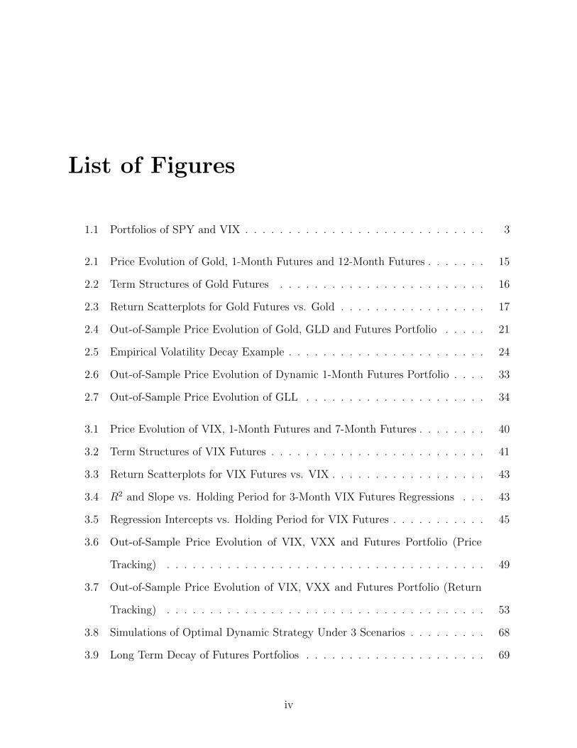
List of Figures iv
List of Tables vi
1 Introduction 1
1.1 Market Mechanism . . . . . . . . . . . . . . . . . . . . . . . . . . . . . . . . 5
1.2 Literature Review . . . . . . . . . . . . . . . . . . . . . . . . . . . . . . . . . 7
2 Tracking Gold with Futures 12
2.1 Gold Spot & Futures . . . . . . . . . . . . . . . . . . . . . . . . . . . . . . . 13
2.1.1 Price Dependency . . . . . . . . . . . . . . . . . . . . . . . . . . . . . 14
2.1.2 Static Replication of Gold Spot Price . . . . . . . . . . . . . . . . . . 18
2.2 Leveraged ETFs . . . . . . . . . . . . . . . . . . . . . . . . . . . . . . . . . . 21
2.2.1 Empirical Leverage Estimation . . . . . . . . . . . . . . . . . . . . . 24
2.2.2 Static Leverage Replication . . . . . . . . . . . . . . . . . . . . . . . 27
2.2.3 Dynamic Leverage Replication . . . . . . . . . . . . . . . . . . . . . . 30
3 Tracking VIX with Futures 35
3.1 VIX Spot & Futures . . . . . . . . . . . . . . . . . . . . . . . . . . . . . . . 36
3.1.1 Return Dependency . . . . . . . . . . . . . . . . . . . . . . . . . . . . 38
3.1.2 Long-Term Dependency . . . . . . . . . . . . . . . . . . . . . . . . . 42
3.1.3 Static Physical Replication . . . . . . . . . . . . . . . . . . . . . . . . 45
i

3.1.4 Static Return Replication . . . . . . . . . . . . . . . . . . . . . . . . 49
3.2 Discrete-Time Model . . . . . . . . . . . . . . . . . . . . . . . . . . . . . . . 54
3.2.1 Futures Portfolio . . . . . . . . . . . . . . . . . . . . . . . . . . . . . 54
3.2.2 Optimal Tracking Problem . . . . . . . . . . . . . . . . . . . . . . . . 58
3.3 Numerical Implementation . . . . . . . . . . . . . . . . . . . . . . . . . . . . 63
3.3.1 Empirical Estimation . . . . . . . . . . . . . . . . . . . . . . . . . . . 64
3.3.2 Qualitative Properties of the Solution . . . . . . . . . . . . . . . . . . 67
4 Dynamic Index Tracking 73
4.1 Continuous-Time Tracking Problem . . . . . . . . . . . . . . . . . . . . . . . 74
4.1.1 Price Dynamics . . . . . . . . . . . . . . . . . . . . . . . . . . . . . . 74
4.1.2 Tracking Portfolio Dynamics . . . . . . . . . . . . . . . . . . . . . . . 76
4.1.3 Portfolios with Futures . . . . . . . . . . . . . . . . . . . . . . . . . . 83
4.2 Equity Index Tracking . . . . . . . . . . . . . . . . . . . . . . . . . . . . . . 86
4.2.1 Black-Scholes Model . . . . . . . . . . . . . . . . . . . . . . . . . . . 86
4.2.2 Heston Model . . . . . . . . . . . . . . . . . . . . . . . . . . . . . . . 92
4.3 Volatility Index Tracking . . . . . . . . . . . . . . . . . . . . . . . . . . . . . 96
4.3.1 CIR Model . . . . . . . . . . . . . . . . . . . . . . . . . . . . . . . . 96
4.3.2 Comparison to VXX . . . . . . . . . . . . . . . . . . . . . . . . . . . 99
4.3.3 CSQR Model . . . . . . . . . . . . . . . . . . . . . . . . . . . . . . . 105
5 Schedule Following in Algorithmic Trading 109
5.1 Optimal Order Type Selection . . . . . . . . . . . . . . . . . . . . . . . . . . 110
5.2 Affine Uncertainty of Limit Orders . . . . . . . . . . . . . . . . . . . . . . . 114
5.2.1 Numerical Illustration . . . . . . . . . . . . . . . . . . . . . . . . . . 118
5.3 Constant Uncertainty of Limit Orders . . . . . . . . . . . . . . . . . . . . . . 123
5.3.1 Trade Direction-Speed Trade-off . . . . . . . . . . . . . . . . . . . . . 124
5.3.2 Optimal Strategies . . . . . . . . . . . . . . . . . . . . . . . . . . . . 125
ii

5.3.3 Buy-Sell Boundary . . . . . . . . . . . . . . . . . . . . . . . . . . . . 126
5.4 Linear Uncertainty of Limit Orders . . . . . . . . . . . . . . . . . . . . . . . 130
5.4.1 Liquidation Penalty and Trading Horizon Trade-off . . . . . . . . . . 130
5.4.2 Infinite Uncertainty Limit . . . . . . . . . . . . . . . . . . . . . . . . 134
5.5 Schedule Following . . . . . . . . . . . . . . . . . . . . . . . . . . . . . . . . 135
Bibliography 140
Appendix 146
A.1 Derivation of SDE (4.1.5) . . . . . . . . . . . . . . . . . . . . . . . . . . . . 146
A.2 Validation of (4.3.10) when Mean-Reversion Speeds are Equal . . . . . . . . 147
A.3 Solution to (4.3.11) when Mean-Reversion Speeds are Equal . . . . . . . . . 148
A.4 Validation of (4.3.10) when Mean-Reversion Speeds are Unequal . . . . . . . 149
iii
List of Figures
1.1 Portfolios of SPY and VIX . . . . . . . . . . . . . . . . . . . . . . . . . . . . 3
2.1 Price Evolution of Gold, 1-Month Futures and 12-Month Futures . . . . . . . 15
2.2 Term Structures of Gold Futures . . . . . . . . . . . . . . . . . . . . . . . . 16
2.3 Return Scatterplots for Gold Futures vs. Gold . . . . . . . . . . . . . . . . . 17
2.4 Out-of-Sample Price Evolution of Gold, GLD and Futures Portfolio . . . . . 21
2.5 Empirical Volatility Decay Example . . . . . . . . . . . . . . . . . . . . . . . 24
2.6 Out-of-Sample Price Evolution of Dynamic 1-Month Futures Portfolio . . . . 33
2.7 Out-of-Sample Price Evolution of GLL . . . . . . . . . . . . . . . . . . . . . 34
3.1 Price Evolution of VIX, 1-Month Futures and 7-Month Futures . . . . . . . . 40
3.2 Term Structures of VIX Futures . . . . . . . . . . . . . . . . . . . . . . . . . 41
3.3 Return Scatterplots for VIX Futures vs. VIX . . . . . . . . . . . . . . . . . . 43
3.4 R2 and Slope vs. Holding Period for 3-Month VIX Futures Regressions . . . 43
3.5 Regression Intercepts vs. Holding Period for VIX Futures . . . . . . . . . . . 45
3.6 Out-of-Sample Price Evolution of VIX, VXX and Futures Portfolio (Price
Tracking) . . . . . . . . . . . . . . . . . . . . . . . . . . . . . . . . . . . . . 49
3.7 Out-of-Sample Price Evolution of VIX, VXX and Futures Portfolio (Return
Tracking) . . . . . . . . . . . . . . . . . . . . . . . . . . . . . . . . . . . . . 53
3.8 Simulations of Optimal Dynamic Strategy Under 3 Scenarios . . . . . . . . . 68
3.9 Long Term Decay of Futures Portfolios . . . . . . . . . . . . . . . . . . . . . 69
iv

3.10 Dynamic Strategy for Tracking VIX . . . . . . . . . . . . . . . . . . . . . . . 70
3.11 Return Scatterplots for Simulated Dynamic Portfolio/VXX vs. VIX . . . . . 71
4.1 Black-Scholes Leveraged Portfolio Tracking . . . . . . . . . . . . . . . . . . . 88
4.2 β = 1 Tracking Strategies for Options and Futures in the Black-Scholes Model 90
4.3 β = −1 Tracking Strategies for Options and Futures in the Black-Scholes Model 91
4.4 Calibrated VIX Futures Term Structures in the SQR Model . . . . . . . . . 98
4.5 Simulation of VIX, VXX, and VXX’s Composite Futures . . . . . . . . . . . 100
4.6 Simulations of VIX, VXX, and β = 1 Tracking Portfolio in the SQR Model . 101
4.7 Return Scatterplots for the Portfolios in Figure 4.6 . . . . . . . . . . . . . . 102
4.8 Implied βt for VXX . . . . . . . . . . . . . . . . . . . . . . . . . . . . . . . . 103
4.9 αt for VXX and Tracking Portfolio in SQR Model . . . . . . . . . . . . . . . 104
4.10 β = 1 Tracking Strategies for 1 and 2-Month Futures in SQR Model . . . . . 105
5.1 Optimal Trading Rates under Constant, Linear and No Uncertainty . . . . . 121
5.2 Optimal Trading Rates with Varied Market Impact . . . . . . . . . . . . . . 122
5.3 Optimal Stock Holdings vs. Time . . . . . . . . . . . . . . . . . . . . . . . . 123
5.4 Buy-Sell Boundary vs. Time with Different Parameters . . . . . . . . . . . . 130
5.5 Optimal Stock Holdings vs. Time (with Schedule) . . . . . . . . . . . . . . . 137
5.6 Optimal Trading Rates with Schedule . . . . . . . . . . . . . . . . . . . . . . 139
v

List of Tables
1.1 Table of Gold (L)ETFs . . . . . . . . . . . . . . . . . . . . . . . . . . . . . . 6
1.2 Table of VIX (L)ETFs . . . . . . . . . . . . . . . . . . . . . . . . . . . . . . 8
2.1 Single Day Return Regressions for Gold Futures . . . . . . . . . . . . . . . . 14
2.2 Multiple Day Return Regressions for Gold Futures . . . . . . . . . . . . . . . 18
2.3 Optimal Gold Tracking Futures Portfolios . . . . . . . . . . . . . . . . . . . 20
2.4 Hypothetical Volatility Decay Example . . . . . . . . . . . . . . . . . . . . . 23
2.5 Single Day Return Regressions of Gold (L)ETFs vs. Gold . . . . . . . . . . . 25
2.6 Multiple Day Return Regressions of Gold (L)ETFs vs. Gold . . . . . . . . . 26
2.7 Gold +2x Optimal Futures Portfolios . . . . . . . . . . . . . . . . . . . . . . 28
2.8 Gold -2x Optimal Futures Portfolios . . . . . . . . . . . . . . . . . . . . . . . 28
2.9 Gold +3x Optimal Futures Portfolios . . . . . . . . . . . . . . . . . . . . . . 29
2.10 Gold -3x Optimal Futures Portfolios . . . . . . . . . . . . . . . . . . . . . . . 29
2.11 Returns and Tracking Errors for Leveraged Dynamic Portfolios . . . . . . . . 33
3.1 Single Day Return Regressions for VIX Futures . . . . . . . . . . . . . . . . 38
3.2 Multiple Day Return Regressions for VIX Futures . . . . . . . . . . . . . . . 44
3.3 Optimal VIX Tracking Futures Portfolios . . . . . . . . . . . . . . . . . . . . 48
3.4 Optimal VIX Return Tracking Futures Portfolios . . . . . . . . . . . . . . . 52
3.5 Regression Results for Figure 3.11 . . . . . . . . . . . . . . . . . . . . . . . . 71
vi

Acknowledgements
First and foremost I must thank my advisor, Tim Leung. Tim has a passion for research
and Financial Engineering that immediately resonated with me upon meeting him. His
research style and dedicated focus is something I strive to attain every day when I begin
work. Without Tim, I would not have been successful in my Ph.D. program and I am forever
grateful to him for showing me how to conduct research.
Next, I would like to thank the other members of my committee: Agostino Capponi, Ton
Dieker, Hongzhong Zhang and Yuchong Zhang. I appreciate them taking the time to sit for
my defense and as well as carefully reading over this thesis.
My academic career has been shaped by a number of amazing teachers, lecturers and
professors. Going all the back to Commack High School, I must thank Derek Pope, Nancy
Pally, Barbara Gerson and Bruce Leon for giving me my mathematical foundation. Whether
it was Math Fair, AP/IB Calculus class, or the Math Team, I always found myself immersed
in what I was doing/learning from them. Next, I dove deeper into the field of mathematics
by studying in the Applied Mathematics and Statistics (AMS) Department at Johns Hopkins
University (JHU). It was there that discovered how useful mathematics is for finance and
found that I wanted to pursue a Ph.D. program while researching Financial Engineering.
Amongst the many faculty who lectured me through my undergraduate and master’s studies
I must thank Jian Kong, Beryl Castello, John Wierman, Daniel Naiman, Donniell Fishkind,
David Audley, Fred Torcaso, Avanti Athreya, and Agostino Capponi. Finally, at Columbia I
had the pleasure of learning the core materials in Optimization and Stochastic Modeling from
vii

Donald Goldfarb, Daniel Bienstock, Ward Whitt and David Yao. Their lectures gave me
new insights into materials already familiar to me as well as introduced me to new branches
of Operations Research in an engaging way.
I also owe gratitude to the various staff at JHU and Columbia that facilitated every step
of the way and brought me to this point in my academic career. They have made sure that
everything went through smoothly so I could focus on my studies and my research. From
JHU I would like to thank Kristen Bechtel and Sandy Kirt. From Columbia I would like
to thank Jaya Mohanty, Krupa Thakore, Adina Brooks, Jenny Mak, Lizbeth Morales, and
Kristen Maynor.
A great education is nothing without friends to share it with. My colleagues at JHU and
Columbia are nothing short of amazing and I’m glad to have worked with them on various
projects and sharing conversations with them about courses. From Johns Hopkins I would
especially thank Jordan Pryor, Matt Molisani and Ilana Bookner, whom I worked with on
my first research project in MiLB Scheduling. At Columbia, I learned a lot from my fellow
students: Jalaj Bhandari, Mauro Escobar, Itai Feigenbaum, Fei He, Randy Jia, Xin Li, Brian
Lu, Cun Mu, and Nouri Sakr. Some of these students served as my TA in various courses
and I am especially grateful to them for helping me along the way. Additionally, I spent a
great deal of time learning from Allen Cheng, Kevin Guo, and Michael Hamilton. I have
known Allen since we met at JHU and we will continue to work together at AQR. Kevin
and I share Tim as an advisor and naturally, we have common intellectual interests. Our
conversations have led to furthering of each other’s projects and I know our collaboration
will never end. Finally, Michael has been one of my closest friends here in the department.
We shared Mudd 323 as an office space for two years and quite often, were the only two
people there. In those times, our friendly banter made this Ph.D. program all the more
enjoyable.
My brothers and sister have always supported every goal I have set and encouraged
everything I work on. My true goal is to be like them and I owe them for setting such high
viii

standards. My brother Steve showed me that anything can be accomplished by working
hard and setting your mind to it. He is dedicated to everything he does and I have learned
from him that with focus, no goal is impossible. Charles, my oldest brother, was the first
person in my life to show me that mathematics could be fun and exciting. I fondly remember
practicing for the Continental Math League with his help when I was in second grade. We
continue to challenge each other to learn more, whether it be mathematics, statistics or
programming. Finally, my sister Jen showed me how to dream big. My mom has told me
many times that when Jen told her that she would like to become a medical doctor, my mom
said, “I don’t think we know how to do that! But let’s find out.” With that story in my
mind, I have always set my mind to big goals, sometimes dreaming up what others would
see as impossible. Achieving those goals required all of their help and support.
A mother will always be your biggest cheerleader. She is the only person in your life who
has literally been cheering you on since day one. There is nothing quite like the smile on
my mom’s face as I tell her about something I am planning on doing, already working on,
or have achieved. My mom has such a pride in me and that pride powers me through every
single tough moment.
Finally, I would like to thank my girlfriend Sara Furia. We have been together for nine
and a half years and she is truly my best friend. She has listened to every stressful moment,
and helped keep me grounded through it all. Because of Sara, I have been able to stay
calm when things seemed impossible to deal with. She always has the right thing to say to
keep me going. I look forward to our life together in Stamford and all that it will bring us.
Although life is unpredictable, one thing is certain: Sara will always be there by my side.
ix

In memory of my father.
x

Chapter 1
Introduction
Many institutional investors seek to control their portfolio’s exposure to various market
factors. Asset managers, hedge funds and other investors must carefully set the exposures of
their portfolio in order to provide the promised returns their clients demand. Recognizing this
need, many major investment funds have issued a number of exchange-traded funds (ETFs),
exchange traded notes (ETNs), and exchange traded products (ETPs) that attempt to give
investors the desired exposure. In addition to these base products, investment funds also
issue leveraged ETFs (LETFs). Such products promise some (possibly negative) multiple of
the daily returns of a reference index or basket of other assets.
However, empirically it has been found that these products can fail to achieve their
stated goals. Moreover, it is often the case that these products lose money relative to those
targets. The reasons for these failures can be attributed to the static or passively dynamic
strategies followed by many of the ETF providers. By passively dynamic, we mean that the
strategy involves a time-deterministic allocation into various assets. Though such strategies
are dynamic, they do not adapt to changing markets. Because of these issues, it is essential
to empirically track and theoretically explain these observed deviations.
The markets for gaining exposure to gold and volatility provide interesting examples for
understanding these deviations. Gold is often viewed by investors as a safe haven or a hedge
against market turmoils, currency depreciation, and other economic or political events (see
1

CHAPTER 1. INTRODUCTION 2
Ghosh et al. (2004) and Baur and McDermott (2010) for empirical investigation of gold’s
role as a safe haven). Gold (L)ETFs are a natural investment vehicle to obtain this hedge in
one’s portfolio. Baur (2013) studies the cost-effectiveness of gold ETFs relative to physical
gold holdings, while Ivanov (2013) studies the tracking errors for gold (as well as silver and
oil) ETFs over the period from March 2009 to August 2009. Both studies find that gold
ETFs are useful in tracking spot gold.
In contrast to the ease of tracking spot gold, tracking the Chicago Board Options Ex-
change’s (CBOE’s) Volatility Index (VIX) has been shown to be quite difficult. VIX ETFs
are typically constructed from a portfolio of futures contracts. However, such futures based
ETFs are not useful for diversification and achieving volatility exposure as demonstrated by
Husson and McCann (2011) and Deng et al. (2012). In particular, the Barclay’s iPath S&P
500 VIX Short-Term Futures ETN (VXX) has significant tracking error with respect to VIX.
This is of course due to the tracking errors of these products. Futures based ETPs and their
tracking errors are studied further by Alexander and Korovilas (2013) and Whaley (2013).
Nonetheless, exposure to VIX gives a similar hedge in that VIX rises in times of market
turmoil. We illustrate the effects of having exposure to VIX by considering the 2011 U.S.
credit rating downgrade by Standard and Poor’s. News of a negative outlook by S&P
of the U.S. credit rating broke on April 18th, 2011.1 A retail investor only holding the
SPDE S&P 500 ETF, SPY (which is a tradable index tracking ETF), could have turned
an unprofitable several months (100 days after the news) into a relatively stable period by
investing a small fraction (10%) of his or her wealth into VIX (see Figure 1.1.) The blue
time series represents the hedged portfolio utilizing VIX, while the purple time series is
unhedged (100% in SPY.) On the left panel, the investment is held from the day after the
above news story through a month past the official downgrade on August 5th, 2011.2 The
hedged portfolio is stable through the downgrade and ends up with a small positive return,
while the unhedged portfolio loses about 10%.
1See New York Times article: http://www.nytimes.com/2011/04/19/business/19markets.html.2See: http://www.nytimes.com/2011/08/06/business/us-debt-downgraded-by-sp.html.

CHAPTER 1. INTRODUCTION 3
Time (Days)0 20 40 60 80 100
Price
85
90
95
100
105
110
SPY w/ VIXSPY
(a) April 2011 - Sept. 2011Time (Days)
0 50 100 150 200 250
Price
95
100
105
110
115
120
SPY w/ VIXSPY
(b) Jan. 2014 - Dec. 2014
Figure 1.1: Hedged portfolios of SPY with 10% fraction of wealth invested in VIX from April19th, 2011 to September 9th, 2011 (left) and all of 2014 (right). The x-axis marks the trading daynumber, while the y-axis marks the price. All portfolios are initialized to $100.
The stability of utilizing VIX can be demonstrated even when there is not much market
turmoil. On the right panel of Figure 1.1 we plot the same pair of portfolios over the entire
2014 calendar year. Though both earn roughly the same 15% return, though the SPY only
portfolio is more volatile than the hedged portfolio. The large drawdowns (for example on
October 15th) are met by rises in VIX thereby stabilizing the portfolio’s value. This hedge
motivates us to understand how to trade in such a way as to mimic the daily returns of VIX
and more general indices or market exposures.
In this thesis, we study the index tracking problem through the use of derivatives con-
tracts. We begin in Chapter 2 with an empirical study of products traded on the mar-
ket related to gold. In particular, we study the spot price, gold futures and various gold
(L)ETFs. There are significant price co-movements amongst these assets. Moreover, we
show that static portfolios consisting of one or two futures with different maturities can
effectively replicate the physical spot gold price. As for leveraged gold ETFs, their average
returns tend to be lower than the corresponding multiple (β ∈ 3, 2,−2,−3) of the spot’s
returns, and the under-performance worsens over a longer holding period. In order to track
the leveraged benchmark, we construct a dynamic leveraged portfolio using the 1-Month
futures. We demonstrate that the portfolio tracks the leveraged benchmark better than the

CHAPTER 1. INTRODUCTION 4
corresponding LETFs, and has better returns over multiple years. Chapter 2 is based on
Leung and Ward (2015).
In Chapter 3, we adopt the same methodology of Chapter 2 to the market for volatility.
However, the results are quite different and we find that VIX is much harder to track. Because
of the mean reverting nature of VIX, VIX futures suffer strongly from roll yield losses and
persistently lose money relative to the benchmark. Thus, static portfolios completely fail
even in the case of tracking the unlevered benchmark. In contrast to the previous chapter,
we also constructs portfolios by optimizing the coefficients with respect to another tracking
criterion. But even in this case, tracking VIX with static portfolios appears completely
impossible. We construct a simple myopic approach, which tracks well in simulation studies,
but when backtested it does not perform well. The results of this chapter, along with the
failure of static portfolios for leveraged exposure in Chapter 2 motivate the need for further
exploration of dynamic strategies.
In Chapter 4, we turn our attention to dynamic strategies. We develop a general frame-
work for understanding index tracking and exposure control using derivatives. The frame-
work is useful for all asset classes as long as that asset class is modeled by a continuous
diffusion process. The exposure control problem is an inverse problem to the dynamic hedg-
ing problem. In that problem, the goal is to dynamically trade one or more underlying assets
in such a way as to replicate the price evolution of the newly created derivative. Of crucial
importance in the dynamic hedging problem is the tradability of the underlying asset. In
the problem that we pose in Chapter 4, the underlying and/or its driving factors may not be
directly traded, but derivatives on the underlying are traded. We use derivatives to replicate
(or more generally, control the exposure to) the underlying asset returns and the factors.
The results of Chapter 4 facilitate our understanding of the successes and failures of
various (L)ETFs. In particular, we can quantify the divergence of portfolio returns from
target (leveraged) returns of the index and its factors via a slippage process, so-named
because it is typically negative. Moveover, we discuss how many well-known models fall into

CHAPTER 1. INTRODUCTION 5
our framework. In particular, we discuss index tracking in the context of the Black-Scholes
and Heston Models, which are typically used for modeling equity prices. We also discuss the
framework in the context of two models typically used for the pricing of VIX derivatives (see
Grubichler and Longstaff (1996) and Mencıa and Sentana (2013)). There, we use VXX as
an example portfolio, and give reasons why VXX can fail to track VIX if indeed VIX follows
the posited dynamics. Chapter 4 is based on Leung and Ward (2017).
In Chapter 5, we consider the low level execution of these trading strategies. This problem
is itself another tracking problem, but of a different kind. In particular, the trader must
choose how to use market and limit orders so as to purchase or liquidate a given asset over
a finite time horizon. In this chapter, we analyze a continuous-time stochastic model for
optimal execution using both order types thereby extending the foundational market impact
model of Almgren and Chriss (2000). In particular, we include fill uncertainty for limit orders
as well as a number of other features: a penalty for incomplete liquidation, a trade director
and a speed limiter. These penalties force the algorithm to trade to full liquidation while
simultaneously tailoring the sign and magnitude of the trading rates. Our key result is the
solution to a stochastic optimal control problem, whose associated nonlinear HJB equation
can be simplified to a system of linear ODEs. The methodology can be applied to tracking a
benchmark schedule of stock holdings as well. This schedule following problem has become
important to many brokerages recently as they seek to execute their clients’ trades while
following specific goals. The results in Chapter 5 are adapted from Bulthuis et al. (2017b),
an abridged version of which was published online in RISK Magazine (see Bulthuis et al.
(2017a)).
1.1 Market Mechanism
Before beginning our study, let us discuss the mechanics of the futures and equity markets
that we analyze empirically in Chapters 2 and 3 and theoretically in Chapter 4. First, gold
futures are exchange-traded contracts written on 100 troy ounces of gold, with a number of

CHAPTER 1. INTRODUCTION 6
available delivery dates within 6 years of any given trading date. In the US, gold futures are
traded at the New York Mercantile Exchange (NYMEX). The available months include the
front three months, every February, April, August and October falling within the next 23
months, and every June and December falling within the next 72 months. Trading for any
specific contract terminates on the third to last business day of the delivery month.3
The gold ETFs and ETNs traded on the market are designed to track the spot price of
gold, and are liquidly traded on exchanges. In fact, the SPDR Gold Trust ETF (GLD), is one
of the most traded ETFs with an average trading volume of 7.96 million shares and market
capitalization of $34.5 billion as of June 2017.4 Besides the spot gold ETF, GLD, there are
also LETFs written on gold. In the gold market, the leverage ratios that exist are are ±2
and ±3. Major issuers include ProShares, iShares, and VelocityShares (see Table 1.1.) For
example, the VelocityShares 3x Long Gold ETN (UGLD) provides a return of 3 times the
gold spot price. Furthermore, one can take a bearish position on the gold spot price by
investing in an LETF with a negative leverage ratio. An example is the VelocityShares 3x
Inverse Gold ETN (DGLD).
LETF Issuer β Fee Inception Date
GLD iShares 1 0.40% November 18th, 2004
UGL ProShares 2 0.95% December 1st, 2008
GLL ProShares −2 0.41% December 1st, 2008
UGLD Janus 3 1.35% October 14th, 2011
DGLD Janus −3 1.35% October 14th, 2011
Table 1.1: A summary of the available gold (L)ETFs. For the LETFs, those with higher absoluteleverage ratios, |β| ∈ 2, 3, have higher expense fees.
In the market for volatility, VIX futures began trading on March 26th, 2004. Naturally,
they provide exposure to volatility and therefore allow for a hedge for the asymmetric volatil-
ity effect. In particular, when equity returns are low, volatility tends to be high (see e.g.
Black (1976)). VIX futures have a contract multiplier of $1,000, meaning that one contract
3Historical quotes and contract specifics of gold futures are obtained from the CME Group http://www.
cmegroup.com/trading/metals/precious/gold_contract_specifications.html.4According to ETF Database http://www.etfdb.com/compare/volume.

CHAPTER 1. INTRODUCTION 7
is worth $1,000 times the quoted futures price. In fact, VIX futures were scaled down by
a factor of 10 on March 26th, 2007. At this point in time, the scaling aligned VIX futures
prices to be in accordance with quoted VIX prices.5 In terms of available maturities, initially
only four existed: the front 3 months and the 6-Month contract. Two years later the CBOE
began to offer more contracts including a 9 and 12-Month contract and for some time a
24-Month contract. At this point in time, the established contracts are more stable and
on any given day there are between seven and nine futures contracts available for trading.
These contracts always consist of the front seven through nine months.6
Just as in the gold market, there are (L)ETFs linked to VIX. However, such (L)ETFs do
not claim to track VIX directly. Instead, the index that these (L)ETFs track (or track some
possibly negative multiple of) is the S&P-500 Short Term VIX Futures Index. Thus, all
(L)ETFs displayed in Table 1.2 consist of a portfolio of short term (1 or 2-Month maturity)
VIX futures just as the index itself does.7 Nonetheless it is the goal of this thesis to better
understand how to properly gain exposure to volatility without being exposed to the well
known losses that portfolios of futures suffer. Thus, we will be benchmarking VIX ETFs to
VIX itself. In fact, in Chapter 3 we will focus our attention on benchmarking the performance
of VXX, but it is useful to know there are other VIX (L)ETFS available, especially those
with β < 0, given the recent downtrend in volatility.8
1.2 Literature Review
Tracking an index has been well studied in the literature from a number of different perspec-
tives. For example, Bamberg and Wagner (2000) demonstrate that regression assumptions
are often violated in the context of index tracking. However, they show that regression anal-
5Refer to http://cfe.cboe.com/publish/CFEinfocirc/CFEIC07-003%20.pdf for details on the rescal-ing.
6See http://cfe.cboe.com/products/spec_vix.aspx. The CBOE states they will list up to nine near-term months for trading.
7See http://us.spindices.com/indices/strategy/sp-500-vix-short-term-index-mcap for detailson S&P-500 Short Term VIX Futures Index.
8See http://www.nytimes.com/2017/05/02/business/dealbook/vix-political-risk.html.

CHAPTER 1. INTRODUCTION 8
LETF Issuer β Fee Inception
VXX iPath 1 0.89% January 29th, 2009
VIIX Janus 1 0.89% November 29th, 2010
XXV iPath −1 0.89% July 16th, 2010
XIV Janus −1 1.35% November 29th, 2010
TVIX Janus 2 1.65% November 29th, 2010
UVXY ProShares 2 0.86% October 3rd, 2011
Table 1.2: A summary of the VIX (L)ETFs. For the LETFs (β ∈ −1, 2), the expense ratios arehigher and for the higher value β = 2, the expense ratio is the highest.
ysis is still a useful tool in some cases, thereby indicating that static portfolios can sometimes
perform well in tracking an index. Assuming a small subset of available stocks each following
a Geometric Brownian Motion, Yao et al. (2006) solve a stochastic linear quadratic control
problem for the optimal stock allocation that best tracks a (constant) benchmark rate of
return. This can be viewed as trying to track the growth rate of, e.g. the S&P 500 using
only a small fraction of its composite stocks. Primbs and Sung (2008) extend this work to
include probabilistic portfolio constraints, e.g. short sale restrictions. By working in discrete
time, they find the optimal allocation via semi-definite programming. A similar problem was
studied by Edirisinghe (2013) from a mean-variance framework. In light of the Markowitz
Portfolio Optimization approach, he considers optimizing a combination of mean and vari-
ance of the portfolio’s tracking error with respect to a benchmark index. This thesis adds
to the index tracking literature through the key results (see Propositions 4.1.2 and 4.1.1) in
Chapter 4. There, we will discuss a continuous diffusion framework to better understand
index tracking and risk exposure control using financial derivatives.
This thesis contributes to the growing literature on ETFs and their leveraged counter-
parts. There are a number of studies on the price dynamics of LETFs, including Cheng and
Madhavan (2009), Avellaneda and Zhang (2010), and Jarrow (2010). They illustrate how
the value of an LETF can erode proportional to the leverage ratio as well as the realized
variance of the reference index. The volatility decay has implications for the long-term in-
vestor. Leung and Park (2016) study such an investor and determine the long-term growth

CHAPTER 1. INTRODUCTION 9
rate of utility of LETFs as well as the optimal leverage ratio for these investors. As we will
see in Chapter 4, there are a number of useful derivative securities for tracking a leveraged
benchmark. A natural one is the LETF option. As options traders often quote values of
options in terms of their implied volatilities, it is crucial to understand the dynamics of the
implied volatilities of LETF options. For work in that direction, we refer to Leung and Sircar
(2015) and Leung et al. (2016b).
There are also a number of empirical studies on (L)ETFs. For equity ETFs, Rompotis
(2011) applies regression to determine the tracking errors between ETFs and their stated
benchmarks, and finds persistence in tracking errors over time. The horizon effect is also
illustrated in the empirical study by Murphy and Wright (2010) for commodity LETFs. Guo
and Leung (2015) systematically study the tracking errors of a large collection of commodity
LETFs. They define a realized effective fee to capture how much an LETF holder effectively
pays the issuer due to the fund’s tracking errors. Furthermore, Holzhauer et al. (2013)
corroborate the volatility effect by using VIX data in a linear regression of the returns.
Additionally, they find that the change in the expected volatility is even more significant in
this regression and that the volatility effect is stronger for bear LETFs than for bull LETFs.
In this thesis, we find a similar effect9 in that it is more difficult to track a negatively leveraged
benchmark than a positively leveraged one. For more related studies on the empirical and
theoretical price dynamics of LETFs, we refer to the book by Leung and Santoli (2016).
Many of the (L)ETFs we consider are futures based so we will be analyzing the tracking
properties of futures portfolios and futures based replication of indices, with a focus on
gold and VIX. For a general overview of commodity ETFs constructed with futures, see
Guedj et al. (2011). Alexander and Barbosa (2008) discuss hedging strategies with futures
contracts for index ETFs and compare them against some minimum variance hedge ratios.
Empirical studies by Baur (2012) and Smales (2015) show that the volatility of gold spot and
futures exhibits asymmetric responses to market shocks. Their studies argue that the higher
9We demonstrate this empirically in Chapters 2 and 3 and discuss theoretical reasons in Chapter 4.

CHAPTER 1. INTRODUCTION 10
sensitivity of gold volatility to positive shocks can be interpreted by the safe haven property
of gold. We have previously mentioned some papers on VIX futures, and portfolios of VIX
futures above, but we list them here for completeness. They include Husson and McCann
(2011) and Deng et al. (2012) as well as Alexander and Korovilas (2013) and Whaley (2013).
The results of this thesis have practical implications for the development of trading
strategies. A simple application of much of this work is to pairs trade the tracking portfolio
against some (L)ETF that purports to track the (possibly leveraged) index. For instance,
Triantafyllopoulos and Montana (2011) model the spread between mean-reverting pairs of
gold and silver ETFs, and develop efficient algorithms for estimating the parameters of this
model for trading purposes. Dunis et al. (2013) develop a genetic programming algorithm for
trading gold ETFs. Leung and Li (2015) analyze the optimal sequential timing strategies for
trading pairs of ETFs based on gold, gold miners, or silver. Additionally, Naylor et al. (2011)
find gold and silver ETFs to be highly profitable ETFs and are able to yield highly abnormal
returns based on filtering strategies. Leung et al. (2016a) study the problem of speculative
investing in futures products under mean reverting models. Via a similar approach, Li (2016)
analyzes the optimal trading strategies for VIX futures under mean reverting models where
the mean reverting parameters are subject to regime switching. Though we do not construct
such trading strategies explicitly, it is a natural extension to this work. The empirical
methodology presented in Chapters 2 and 3 can be applied to nearly any asset class and
Chapter 4 allows for better understanding of how profitable such a pairs trade might be.
As for our algorithmic trading model presented in Chapter 5, there are a number of related
studies in the optimal execution and market making literature. The foundational studies
by Bertsimas and Lo (1998) and Almgren and Chriss (2000) began the study of optimal
execution from an academic perspective and our work continues this academic study. There
are a number of related studies on optimal liquidation with similar basic settings as in these
papers, though liquidation with both market and limit orders has only come to the forefront
of the algorithmic trading literature in recent years. Cheng et al. (2017) extend the Almgren-

CHAPTER 1. INTRODUCTION 11
Chriss model to include uncertain order fills of a single order type. Chapter 5 extends
this model even further to include both market and limit orders, along with additional
penalties to guide the trade direction and limit order size. In the case of infinite uncertainty,
our framework captures their model as a special case, with our optimal market order rate
coinciding with theirs. Cartea and Jaimungal (2015) also solve an optimal execution problem
with market and limit orders. Unlike our model, which is based on continuous diffusion
processes, their model uses jump processes and optimal multiple stopping to determine the
optimal market order placement time. They too penalize deviations from a schedule.
Tracking problems in algorithmic trading are important as practictioners seek to follow
benchmark schedules over time. For a specific example of schedule following, we refer to a
recent study by Cartea and Jaimungal (2016). They derive a closed-form optimal strategy
that follows a volume weighted average price (VWAP) schedule. In additon, market making
itself is a type of tracking problem in that the trader seeks to track a position that is low risk
or potentially profitable (from future executions). Market making involves simultaneously
determining the prices and quantities to buy and sell a stock. The market maker receives the
spread in exchange for the risk of holding a position. Avellaneda and Stoikov (2008) apply
indifference pricing techniques to find the optimal quotes for a risk-averse investor trading
over a finite period. Guilbaud and Pham (2013) study a market making problem via the
optimal placement of limit orders as well as using market orders to balance inventory risk.
For more related studies on algorithmic trading and market microstructure, we refer to the
books by Lehalle and Laruelle (2013) and by Cartea et al. (2015).

Chapter 2
Tracking Gold with Futures
In this chapter, we begin our study of index tracking with an empirical investigation of the
tracking performance for spot gold of various securities whose values are tied to gold. In
particular, in Section 2.1, we investigate the price relationships amongst gold LETFs, gold
futures and the gold spot price. Our results show that gold futures are highly correlated
amongst each other and correlated with the spot price of gold. Thus, we find that gold futures
are highly effective in tracking spot gold through static portfolios and that the market traded
ETF (GLD) also exhibits similar tracking performance. On the other hand, we find in Section
2.2 that leveraged gold ETFs tend to underperform their corresponding leveraged benchmark
with worsening underperformance over longer holding periods. The underperformance is even
worse for static portfolios of gold futures. This motivates our study of dynamic portfolios for
index tracking and we analyze one such strategy in Section 2.2.3. We find that the dynamic
portfolio also consistently outperforms the respective market-traded LETFs for different
leverage ratios.
12

CHAPTER 2. TRACKING GOLD WITH FUTURES 13
2.1 Gold Spot & Futures
We begin by analyzing the price dynamics of gold futures with respect to the spot. One
benchmark for the spot gold price are the London Gold Fixing Indices, GOLDLNAM and
GOLDLNPM. Each of these indices is only updated once per business day: 10:30 AM for
GOLDLNAM, and 3:00 PM for GOLDLNPM in London times, by four members of the
London Bullion Market Association (Scotia-Mocatta, Barclays Bank, HSBC, and Societe-
Generale).1 Another widely used benchmark for the gold spot price is the Gold-U.S. Dollar
exchange rate (XAU-USD). It indicates the U.S. dollar amount required to buy or sell one
troy ounce of gold immediately. XAU-USD is frequently updated around the clock and its
closing price is available for all trading days studied from December 22nd, 2008 through July
14th, 2014. For these reasons, we choose XAU-USD as our benchmark for the gold spot price
throughout this chapter.
In the gold futures market, the front months, such as the 1-Month and 2-Month contracts,
are actively traded daily. However, other available contracts are set to expire in specific
calendar months within the next few years. As such, it may not always be possible to trade
6-Month and 12-Month futures, and one may need to alternate with the nearest month. For a
6-Month futures position we assume a position which alternates between 6-Month futures and
5-Month futures and for a 12-Month futures position we assume a position which alternates
between 12-Month futures and 11-Month futures. This involves simply waiting while the
6-Month futures (resp. 12-Month) futures becomes a 5-Month futures (resp. 11-Month)
after one month and then rolling the position forward 2 months after the second month
passes. For example, if it now January 2012 a 12-Month futures contract would be the Dec-
12 contract. When February 2012 comes by, this becomes an 11-Month contract, but the
Jan-13 contract is not available. Instead, we hold the position as an 11-Month futures and
then in March 2012, we roll the position forward into the Feb-13 contract returning it to
1According to the London Bullion Market Association. See http://www.lbma.org.uk/
pricing-and-statistics.

CHAPTER 2. TRACKING GOLD WITH FUTURES 14
a 12-Month position. Throughout this chapter, we will use the 1, 2, 6, and 12-Month gold
futures contracts in our regressions.
2.1.1 Price Dependency
We begin by performing linear regressions of the 1-day returns of spot gold versus the
futures of maturities: 1, 2, 6, and 12-Months. Across all maturities, the linear relationships
are all strong and they are quite similar. In Table 2.1, we summarize the regression results,
including the slope, intercept, R2, and root mean squared error (RMSE). The R2 values are
all greater than 80%, indicating a strong linear fit. For every maturity, the slope is close
to 0.94 and the intercept is essentially zero. The slopes suggest that the price sensitivity of
futures with respect to the spot is slightly less than 1 to 1. While this may suggest that the
futures prices should be less volatile than the spot return, we find that the historical annual
volatilities of the futures are higher: 19.261% (1-Month), 19.263% (2-Month), 19.269% (6-
Month), and 19.266% (12-Month), as compared to the spot (18.374%). The fact that the
regression results are almost the same among different futures suggests that the futures prices
are highly positively correlated. Indeed, our calculations show that the correlation among
the futures over the same period are all over 99%.
Response Slope Intercept R2 RMSE
1-Month 0.94314 2.41916 · 10−5 0.80947 0.00530
2-Month 0.94301 6.20316 · 10−5 0.80911 0.00530
6-Month 0.94348 3.17973 · 10−5 0.80934 0.00530
12-Month 0.94358 −5.23334 · 10−5 0.80984 0.00529
Table 2.1: A summary of the regression coefficients and measures of goodness of fit for regressing1-day returns of 1, 2, 6 and 12-Month futures on 1-day returns of spot gold from December 22nd,2008 to July 14th, 2014.
The high correlation among futures prices can also be seen from their time series. In
Figure 2.1, we plot the gold price, 1-Month futures price (Jan-13 contract) and 12-Month
futures price (Dec-13 contract) over the period from December 29th, 2012 to January 1st,

CHAPTER 2. TRACKING GOLD WITH FUTURES 15
2013. Over this period the 1-Month futures and 12-Month futures prices move in parallel to
one another just as the near perfect correlation would indicate. Furthermore, the gold spot
price and 1-Month futures price are close, as expected. On Jan 29th, 2013, or trading day 21
in Figure 2.1, the 1-Month futures would expire. We observe a slight discrepancy between
the futures price and the spot on this date. While futures should theoretically converge to
the spot price at maturity, in practice gold futures settle at their volume weighted average
(VWAP) price within the last one minute.2 The last price will be equal to the spot price
at maturity, but the settlement price (which is used in marking futures positions to market)
used here will be calculated by weighting this last price against its volume traded and hence
need not be equal to the spot gold price.
Trading Days
Pri
ce
1 2 3 4 5 6 7 8 9 10 11 12 13 14 15 16 17 18 19 20 21
1640
1650
1660
1670
1680
1690
1700
1710Spot1−Month12−Month
Figure 2.1: Time evolution of spot gold price, 1-Month futures price (Jan-13 contract) and 12-Month futures price (Dec-13 contract) over the period from Dec 29th, 2012 to Jan 29th, 2013. Thetwo futures prices move in parallel, and the spot price trades very close to the 1-Month futuresprice. The x-axis marks the trading day number, while the y-axis marks the price.
In fact, the price co-movement among futures also has implications for the term structure
dynamics. On a typical date in the gold market, futures prices are increasing and convex
with respect to maturity as seen in Figure 2.2. Since the futures contracts tend to move in
2According to CME Group gold futures settlement procedures documentation, available at http://www.cmegroup.com/trading/metals/files/daily-settlement-procedure-gold-futures.pdf

CHAPTER 2. TRACKING GOLD WITH FUTURES 16
Time to Maturity (Years)
Pri
ce
Jan. 29Feb. 26Mar. 30April 29May 28June 29
0 1 2 3 4 5
890
910
930
950
970
990
1010
1030
1050
1070
(a) Jan.-June 2009Time to Maturity (Years)
Pri
ce
Jan. 30Feb. 27Mar. 27April 29May 30June 27
0 1 2 3 4 5 6
1200
1240
1280
1320
1360
1400
1440
1480
1520
1560
1600
1640
1680
1720
1760
1800
(b) Jan.-June 2013
Figure 2.2: Term structures from Jan. to June in 2009 (left) and 2013 (right). The legendmarks the date upon which the term structure is constructed (which is one day after that month’sexpiring contract’s maturity). The x-axis marks the time-to-maturity (in years, assuming each yearis precisely 252 days), while the y-axis marks the price.
parallel, this leads to almost parallel shifts in the term structure. The shape of the term
structure remains almost the same over time. During both periods we can see the increasing
convex feature of the gold futures market, but in 2013 there is a reduction in convexity. In
2009, the term structure generally shifts upward from January to June, while in 2013 the
term structure strictly shifts downward from January to June.
Next, we compare the linear relationships for returns computed over 5, 10, and 15 trading
days. Since we use disjoint time windows for return calculations, a longer holding period
implies fewer data points for the regression. In Figure 2.3, we plot the regressions of 12-Month
futures returns versus gold returns for both 1-day returns and 10-day returns, plotted on the
same x-y axis scale. We can see the returns vary on a larger range for the 10-day returns.
Spot gold has a 1-day return between −9.07% (April 15th, 2014)3 and 4.99% (January 23rd,
2009), while its 10-day returns vary between −9.12% (June 6th, 2013 to June 19th, 2013) and
11.30% (August 5th, 2011 to August 18th, 2011). On the other hand, the 12-Month futures
has a 1-day return between −9.40% (April 15th, 2014) and 7.68% (March 19th, 2009), while
3Gold returns plummeted on this day. See http://mobile.nytimes.com/blogs/dealbook/2013/04/
15/golds-plunge-shakes-confidence-in-a-haven/

CHAPTER 2. TRACKING GOLD WITH FUTURES 17
its 10-day returns vary between −9.16% (June 6th, 2013 to June 19th, 2013) and 11.30%
(August 5th, 2011 to August 18th, 2011). Moreover, we can see that the slope is slightly
higher for the 10-day returns versus the 1-day returns.
−0.1 −0.05 0 0.05 0.1 0.15−0.1
−0.05
0
0.05
0.1
0.15
Gold Returns
12−
m F
utu
res R
etu
rns
(a) 1-day Returns
−0.1 −0.05 0 0.05 0.1 0.15−0.1
−0.05
0
0.05
0.1
0.15
Gold Returns
12−
m F
utu
res R
etu
rns
(b) 10-day Returns
Figure 2.3: Linear regressions of 12-Month futures returns based on 1-day returns (left) and 10-day returns (right) versus the spot gold returns. The x-axis marks the returns (decimals, notpercentages) of spot gold, while the y-axis marks the returns (decimals, not percentages) of the12-Month futures.
This is confirmed numerically and in general for the various futures contracts in Table
2.2. Here, we give the slopes for the regression of each futures return versus the gold return,
while varying the holding period. We display the slopes and R2 values from Table 2.1 for
comparison. However, we do not give the intercepts for these regressions as they are all very
trivial and effectively 0. We can see that the slopes approach the value 1 as the holding
period is lengthened. Thus, the longer the holding period, the more closely the gold return
and futures price return are to one another. In particular, the slopes for 10-day returns are
all greater than 1, indicating an increased price sensitivity. Furthermore, the strength (as
measured by R2) of this linear relationship increases with increasing holding period length.

CHAPTER 2. TRACKING GOLD WITH FUTURES 18
Days 1-Month 2-Month 6-Month 12-Month
Slope 1 0.94314 0.94301 0.94348 0.94358
5 0.99805 0.99752 0.99757 0.99715
10 1.01075 1.01020 1.00970 1.00841
15 0.99448 0.99461 0.99431 0.99345
R2 1 0.80947 0.80911 0.80934 0.80984
5 0.97154 0.97158 0.97194 0.97165
10 0.98516 0.98530 0.98572 0.98550
15 0.98704 0.98691 0.98725 0.98713
Table 2.2: A summary of the slopes and R2 from the regressions of futures returns versus goldreturns over different holding periods.
2.1.2 Static Replication of Gold Spot Price
In this section we consider replication of the gold spot price with a static portfolio of futures
contracts. We use portfolios of either 1 or 2 futures contracts and an investment in the
money market account. We seek a static portfolio that minimizes the sum of squared errors:
SSE =n∑j=1
(Vj −Gj)2 , (2.1.1)
where Vj is the dollar value of the portfolio on trading day j, while Gj is the dollar value of
the gold spot price on trading day j.
Let k be the number of futures contracts and w := (w0, . . . , wk) be the real-valued vector
of portfolio weights. In particular, w0 represents the weight given to the money market
account. To calculate the optimal portfolio value we will choose weights historically which
minimize SSE over the 5-year period December 22th, 2008 to December 22th, 2013. Thus,
we solve the following constrained least squares optimization problem:
minw∈Rk+1
‖Cw− d‖2
s.t.k∑j=0
wj = 1.
(2.1.2)

CHAPTER 2. TRACKING GOLD WITH FUTURES 19
The matrix C contains as columns, the historical prices of the various futures contracts
and the money market account,4 and the vector, d contains the historical prices of spot gold.
When we refer to historical prices of say, the 1-Month futures contract, we mean a position
that is rolled forward every contract period. For example, for the 1-Month contract we
begin with an investment of $1, 000 dollars and purchase as many units of 1-Month futures
as possible with this sum. After that contract expires, we roll forward whatever value is left
in the position into the current 1-Month futures. (Previously, this contract was the 2-Month
futures at time 0.) This is similarly defined for 2-Month, 6-Month and 12-Month futures.
All prices are normalized by $1, 000, without loss of generality, so that an investor starting
with $1, 000 will invest $1, 000 · wj into the jth futures contract and $1, 000 · w0 into the
money market account.
We will compare our portfolios to investments in the ETF GLD, which tracks the gold
spot price. To do this, we will perform an out-of-sample analysis and compare the values
of $1000 invested in GLD and $1000 invested in our constructed portfolio over the period
from December 23th, 2013 to July 14th, 2014. To measure the performance we will use the
following root mean squared error for both in-sample and out-of-sample prices:
RMSE =
√√√√ 1
n
n∑j=1
(Vj −Gj)2 . (2.1.3)
We solve this optimization problem for ten different portfolios with one or two fu-
tures, along with the money market account. The optimal weights, and corresponding in-
sample/out-of-sample RMSEs are given in Table 2.3. In general, the money market account
is used minimally as the weights on the account are less than 7% in absolute value for all
ten portfolios.
For all the portfolios with two futures contracts, the optimal strategy is to go long the
shorter term futures contract and short the longer term futures contract, with different
4We use historical overnight LIBOR to construct an investment in the money market account.

CHAPTER 2. TRACKING GOLD WITH FUTURES 20
weights. The sum of the two resulting weights is approximately 1. In terms of RMSE, the
1-Month futures contract appears to be the best replicating instrument of the gold spot.
When it is used alone, it performs best relative to other single futures portfolios. When it is
used in a pair with another futures, it performs better than any other single futures contract,
and better than all other futures pairs: (2-m, 6-m), (2-m, 12-m), and (6-m, 12-m).
Futures w0 w1 w2 RMSE (in) RMSE (out)
1 Futures 1-m −0.01071 1.01071 - 6.62989 3.34047
2-m −0.04835 1.04835 - 12.22148 6.12074
6-m −0.05030 1.05030 - 13.23663 5.33971
12-m −0.06842 1.06842 - 15.11103 5.71318
2 Futures 1-m, 2-m −0.00088 1.27315 −0.27227 6.26711 2.79411
1-m, 6-m −0.00171 1.23899 −0.23729 6.27232 2.97602
1-m, 12-m −0.00021 1.19336 −0.19315 6.28735 3.00006
2-m, 6-m −0.04079 5.06602 −4.02523 10.27413 9.37292
2-m, 12-m −0.01179 2.94860 −1.93681 9.65705 7.08414
6-m, 12-m 0.01481 4.80979 −3.82460 9.57938 4.52846
Table 2.3: A summary of the weights and in/out-of-sample RMSEs for portfolios of one and twofutures contracts. For portfolios with two futures, the weight on the shorter term futures is w1.For portfolios with a single futures, we have w2 = 0. The weight assigned to the money marketaccount is denoted by w0.
In the sample, the RMSE values for the futures portfolios range from 6.63 to 15.11.
Since these values are based on a $1000 investment, this means the error within the sample
is between 0.663% and 1.511%, which is quite low. By comparison, our calculations give a
RMSE of 2.091% for the gold ETF (GLD) during December 22th, 2008 to December 22th,
2013. Over this longer horizon of 5 years, our portfolios track the benchmark better than
GLD. However, over the shorter, out-of-sample period, December 23th, 2013 to July 14th,
2014, GLD appears to track spot gold slightly better. The RMSE value for GLD during
this period is 0.128%, whereas our best portfolio gives a RMSE of 0.279%. In Figure 2.4,
we show the time series of the optimal static portfolio with the 1-Month futures (top), and
the time series for GLD. It is visible that both track the gold spot price closely over this
out-of-sample period.

CHAPTER 2. TRACKING GOLD WITH FUTURES 21
0 20 40 60 80 100 120 140980
1000
1020
1040
1060
1080
1100
1120
1140
1160
Trading Days
Price
Portfolio
Spot
(a) Portfolio with 1-Month Futures
0 20 40 60 80 100 120 140980
1000
1020
1040
1060
1080
1100
1120
1140
1160
Trading Days
Price
GLD
Spot
(b) GLD
Figure 2.4: Out-of-sample time series of our optimal portfolio of 1-Month futures and moneymarket account (top) compared to the spot price, and GLD compared to the spot price (bottom).The x-axis marks the trading day number which is from December 23th, 2013 to July 14th, 2014,while the y-axis marks the price. All portfolios are normalized to start at $1,000.
2.2 Leveraged ETFs
In this section we analyze the returns and tracking performances of various leveraged ETFs.
From historical prices of each LETF, we conduct an estimation of the leverage ratio, and
investigate the potential deviation from the target leverage ratio. Moreover, we construct
a number of static portfolios with futures contracts to seek replication of some leveraged
benchmarks. However, the static portfolios fail to effectively track the leveraged benchmarks.
This motivates us to consider a dynamic portfolio with futures, which turns out to have a
much better tracking performance.

CHAPTER 2. TRACKING GOLD WITH FUTURES 22
By design, an LETF seeks to provide a constant multiple of the daily returns of an
underlying index or asset. Let us denote β ∈ −3,−2,+2,+3 the leverage ratio stated by
the LETF, and Rj the daily return of the underlying (gold spot). Ideally, the LETF value
on day n, denoted by Ln, is given by
Ln = L0 ·n∏j=1
(1 + β Rj). (2.2.1)
We call this the leveraged benchmark, and examine the empirical performance of various
LETFs with respect to this benchmark.
For many investors, one appeal of LETFs is that leverage can amplify returns when the
underlying is moving in the desired direction. Mathematically, we can see this as follows.
Rearranging (2.2.1) and taking the derivative of the logarithm, we have
d
dβ
(log
(LnL0
))=
n∑j=1
Rj
1 + β Rj
. (2.2.2)
With a positive leverage ratio β > 0, if Rj > 0 for all j, then log(LnL0
), or equivalently
the value Ln, is increasing in β. In other words, when the underlying asset is increasing in
value, a larger, positive leverage ratio is preferred. On the other hand, if Rj < 0 for all j,
and β < 0, a more negative β increases log(LnL0
)and thus Ln. This means that when the
underlying asset is decreasing in value, a more negative leverage ratio yields a higher return.
The example below illustrates the consequences of maintaining a constant leverage in an
environment with non-directional movements:

CHAPTER 2. TRACKING GOLD WITH FUTURES 23
Day ETF %-change +2x LETF %-change −2x LETF %-change
0 100 - 100 100 -
1 98 −2% 96 -4% 104 4%
2 99.96 2% 99.84 4% 99.84 −4%
3 97.96 −2% 95.85 −4% 103.83 4%
4 99.92 2% 99.68 4% 99.68 −4%
5 97.92 −2% 95.69 −4% 103.67 4%
6 99.88 2% 99.52 4% 99.52 −4%
Table 2.4: A hypothetical example of how volatility decay can lead to both a long and shortleveraged ETF to losing money, even in the case of perfect daily return tracking.
Even though the ETF records a tiny loss of 0.12% after 6 days, the +2x LETF ends up
with a loss of 0.48%, which is greater (in absolute value) than 2 times the return (−0.12%) of
the ETF. We can see this to be the case on any day (e.g. not just the terminal date) except
for day 1. For example, on day 3, the ETF has a net loss of 2.04% and the LETF has a net
loss of 4.15%, which is greater (in absolute value) than 4.08% (twice the absolute value of
the return of the ETF). Furthermore, it might be intuitive that that the −2x LETF should
have a positive return when the ETF and LETF have negative returns: this is not true. At
the terminal date, both the long and short LETFs have recorded net losses of 0.48%. Again,
this occurs throughout the period as well, not just the terminal date. In addition to day 6,
both the long and short LETFs as well as the ETF itself are in the black. These results are
consequences of volatility decay.
Although long and short LETFs are expected to move in opposite directions daily by
design, it is often possible for both LETFs to have negative cumulative returns when held
over a longer horizon. Figure 2.5 shows the historical cumulative returns of the gold LETFs
UGL (+2x) and GLL (−2x) from July 2013 to July 2014. From trading day 124 (January
24th, 2014) onward, GLL has a negative cumulative return. There are points after trading
date 124 where UGL also has a negative cumulative return. In fact, it starts in the black
on this date and continues to have a net loss until trading date 146 (February 12th, 2014).
This occurs again a few times, another long stretch where both have a net loss is trading

CHAPTER 2. TRACKING GOLD WITH FUTURES 24
date 210 (May 15th, 2014) through 233 (June 18th, 2014).This observation, though perhaps
counter-intuitive at first glance, is a consequence of daily replication of leveraged returns.
The value erosion tends to accelerate during periods of non-directional movements.
0 50 100 150 200 250−0.25
−0.2
−0.15
−0.1
−0.05
0
0.05
0.1
0.15
0.2
0.25
Trading Days
LE
TF
Cum
ula
tive R
etu
rns
UGL
GLL
Zero
Figure 2.5: UGL (+2x) and GLL (−2x) cumulative returns from July 2013 to July 2014. Observethat both UGL and GLL can give negative cumulative returns (below the dotted line of 0%)simultaneously over several periods in time. The x-axis marks the trading day number, while they-axis marks the cumulative return, which is initialized to 0.
2.2.1 Empirical Leverage Estimation
We conduct a regression analysis and the results are given in Table 2.5. Each slope is
approximately equal to the LETF’s target leverage ratio. In principle, if each (L)ETF is
able to generate the desired multiple of daily returns, the slopes of the regression should be
equal to the various leverage ratios. In this table, we give an additional two columns for the
t-statistic and p-value for testing the hypothesis: H0 : slope = β vs. H1 : slope 6= β,
where, β is the target leverage ratio. We can see that each p-value is larger than 0.05 and
therefore conclude that statistically, each (L)ETF does not differ from its target leverage
ratio. This demonstrates to us that the (L)ETFs are performing exactly as desired, at least
on a daily basis.

CHAPTER 2. TRACKING GOLD WITH FUTURES 25
(L)ETF Slope Intercept t-stat p-value R2 RMSE
GLD 1.00540 −1.64276 · 10−5 1.42692 0.15382 0.98060 0.00163
UGL 2.00572 −1.31073 · 10−4 0.73319 0.46357 0.97930 0.00337
GLL -2.00556 −1.05504 · 10−4 0.67089 0.50240 0.97673 0.00358
UGLD 2.99358 −1.98605 · 10−4 0.45211 0.65133 0.98484 0.00421
DGLD -2.97528 −1.69127 · 10−5 0.97442 0.33019 0.95256 0.00752
Table 2.5: A summary of the regression coefficients and measures of goodness of fit for regressing1-day returns of (L)ETFs versus spot gold. We include two additional columns for the t-statisticand p-value for testing the hypothesis that the slope equals the leverage ratio in each case.
We see also that the R2 values for each regression are quite high, all above 95%. For a
fixed |β| ∈ 2, 3, the short LETF tends to have a higher RMSE and lower R2 value than
its corresponding long LETF. Finally, we see in general that as the leverage ratio increases
in absolute value, there is a higher RMSE. One possible explanation is that the benchmark
is leveraged, and this could magnify the tracking error.
Just as in Section 2.1.1, we analyze the effects of changing the holding period. In Table
2.6 we give the slopes and intercepts for the regressions of each (L)ETF’s return versus the
spot return while varying the holding period between 15 and 5 days. Our computations
show the R2 values are all above 95%. We can see that the slopes all approximately equal
the target leverage ratio of the (L)ETF. However we notice that in general the intercepts
get more negative as the holding period is lengthened. Although they are still quite small,
they become more significant as the holding period increases. Our calculations show that the
p-values for testing the hypothesis: H0 : intercept = 0 vs. H1 : intercept 6= 0 generally
tend to decrease for each (L)ETF. In fact, for UGL the intercepts turn out to be statistically
different from 0 (at the 5% level) for holding periods of 3, 4 and 5 days with p-values of
1.37%, 0.57% and 0.33%, respectively. This is consistent with the volatility decay discussed
above. We saw there an example where over shorter periods, the LETF tracks its leverage
ratio well, but over a longer period it tends to lose money when there is high volatility. The
intercepts being different from 0 is akin to the volatility decay in the following sense. Over
longer periods, the regressions show that we require more information than just the gold

CHAPTER 2. TRACKING GOLD WITH FUTURES 26
return to predict the LETF return.
To compare the performance of the LETF versus the target multiple of the spot return,
we also report in Table 2.6, the average return differential, defined by
RD =1
m
m∑j=1
(R
(L)j − β ·R
(G)j
), (2.2.3)
where m is the number of the periods, R(L)j is the LETF’s return over the holding period
and R(G)j is the spot’s return over the holding period. We find this to be increasing (in
absolute value) with the holding period length. That is, as we hold the LETF longer, it
tends to increasingly underperform with respect to the multiple of the underlying return, on
average. This is exactly the same notion described above, since over time, the volatility of
the underlying causes the LETF to erode in value.
Days UGL GLL UGLD DGLD GLD
Slope 1 2.00572 -2.00556 2.99160 -2.96362 1.00540
2 2.00828 -2.00395 2.92015 -3.02429 1.00477
3 1.97770 -1.99661 2.94520 -3.06690 0.99194
4 2.00071 -2.00908 2.97854 -3.04311 1.00206
5 2.02081 -2.03273 2.89478 -3.07267 1.01039
Intercept (·10−4) 1 -1.31074 -1.05505 -1.98605 -0.16913 -0.16428
2 -2.73282 -2.28807 -4.23120 -1.81545 -0.33388
3 -4.06417 -3.96629 -4.97993 -1.05631 -0.40843
4 -5.44427 -4.62166 -8.08478 -2.69971 -0.66133
5 -6.81614 -4.82805 -8.03417 -0.30766 -0.92359
RD (·10−3) 1 -0.12892 -0.10760 -0.19673 -0.02414 -0.01439
2 -0.26677 -0.23191 -0.43999 -0.19081 -0.02964
3 -0.43253 -0.39265 -0.53511 -0.08462 -0.05028
4 -0.54331 -0.47645 -0.81687 -0.27854 -0.06290
5 -0.64076 -0.54705 -0.79183 0.07165 -0.07195
Table 2.6: A summary of the slopes and intercepts from the regressions of LETF returns versusgold returns, as well as the average return differential (RD) over different holding periods.

CHAPTER 2. TRACKING GOLD WITH FUTURES 27
2.2.2 Static Leverage Replication
In this section, we perform the same optimization as in Section 2.1.2. We once again seek a
static portfolio of futures which minimizes SSE. Let k be the number of futures contracts and
w := (w0, . . . , wk) be the real-valued vector of portfolio weights. As before, w0 represents
the weight given to the money market account. We seek the weights which minimize SSE
over the 5-year period from December 22th, 2008 to December 22th, 2013. Thus, we are led
to the same constrained least squares optimization problem we proposed in Section 5.2.1:
minw∈Rk+1
‖Cw− L‖2
s.t.k∑j=0
wj = 1.
(2.2.4)
Again, the matrix C contains as columns, the historical prices of the various futures
contracts and the money market account. Here, the vector L contains the historical prices
of the leveraged benchmark in (2.2.1). Without loss of generality, we normalize the prices
by $1000 so that our solution will give us a set of weights on each instrument.
We will compare the tracking error of our optimal portfolios to that of investments in the
LETFs. To be able to analyze the portfolios we get by solving the optimization problem,
we will perform an out-of-sample analysis over the period from December 23th, 2013 to July
14th, 2014 and see how $1, 000 invested in the LETFs and $1, 000 invested in our optimal
portfolios perform in tracking the leveraged benchmark. To quantify the performance we
use the same root mean square error
RMSE =
√√√√ 1
n
n∑j=1
(Vj − Lj)2, (2.2.5)
where, Vj is the dollar value of the portfolio on trading day j, and now Lj is defined as the
dollar value of the leveraged benchmark on trading day j. Now, we present the results for
the optimization and in-sample/out-of-sample RMSE.

CHAPTER 2. TRACKING GOLD WITH FUTURES 28
UGL(+2x) Futures w0 w1 w2 RMSE (in) RMSE (out)
1 Futures 1-m −1.48159 2.48159 - 153.20152 41.48530
2-m −1.57601 2.57601 - 140.41254 49.56627
6-m −1.58107 2.58107 - 138.63116 47.45953
12-m −1.62627 2.62627 - 134.50683 48.29851
2 Futures 1-m, 2-m −1.94496 −9.89441 12.83937 114.30949 81.36970
1-m, 6-m −1.91184 −8.43451 11.34634 113.67580 67.39428
1-m, 12-m −2.02222 −6.92791 9.95013 108.29897 67.15776
2-m, 6-m −1.64536 −34.26195 36.90731 126.62074 22.64952
2-m, 12-m −1.99096 −18.99151 21.98248 111.75046 40.92852
6-m, 12-m −2.24344 −35.66917 38.91260 102.86283 62.53830
Table 2.7: A summary of the weights and in/out-of-sample RMSEs for portfolios of 1 and 2 futurescontracts which attempt to replicate a leveraged benchmark with β = 2. By comparison, the +2xLETF, UGL has an out-of-sample RMSE of only 5.52485.
GLL(−2x) Futures w0 w1 w2 RMSE (in) RMSE (out)
1 Futures 1-m 1.97544 −0.97544 - 152.33349 76.14381
2-m 2.01068 −1.01068 - 155.76147 73.14698
6-m 2.01234 −1.01234 - 156.43931 74.00595
12-m 2.02926 −1.02926 - 158.06790 73.79237
2 Futures 1-m, 2-m 1.69510 −8.46293 7.76783 139.27436 100.10091
1-m, 6-m 1.70510 −7.83463 7.12954 137.98773 92.21120
1-m, 12-m 1.60773 −7.37540 6.76767 133.31705 93.11206
2-m, 6-m 1.93900 −39.08635 38.14735 142.57324 43.40713
2-m, 12-m 1.57681 −23.56157 22.98477 127.90630 62.10415
6-m, 12-m 1.27887 −43.36906 43.09020 117.81839 88.35987
Table 2.8: A summary of the weights and in/out-of-sample RMSEs for portfolios of 1 and 2 futurescontracts which attempt to replicate a leveraged benchmark with β = −2. By comparison, the −2xLETF, GLL has an out-of-sample RMSE of only 4.76269.

CHAPTER 2. TRACKING GOLD WITH FUTURES 29
UGLD(+3x) Futures w0 w1 w2 RMSE (in) RMSE (out)
1 Futures 1-m −3.33704 4.33704 - 555.49151 111.51133
2-m −3.50625 4.50625 - 529.90858 125.98635
6-m −3.51562 4.51562 - 526.58448 122.33175
12-m −3.59587 4.59587 - 518.96896 123.83019
2 Futures 1-m, 2-m −5.18147 −44.92498 51.10645 379.11676 270.58292
1-m, 6-m −5.02680 −38.53507 44.56188 381.92109 213.62168
1-m, 12-m −5.41970 −31.91076 38.33046 366.49764 210.91245
2-m, 6-m −3.78077 −141.31534 146.09611 472.32904 48.04126
2-m, 12-m −5.12561 −79.66101 85.78662 413.19682 98.33728
6-m, 12-m −6.14011 −147.04408 154.18419 376.40048 185.87170
Table 2.9: A summary of the weights and in/out-of-sample RMSEs for portfolios of 1 and 2 futurescontracts which attempt to replicate a leveraged benchmark with β = 3. By comparison, the +3xLETF, UGLD has an out-of-sample RMSE of only 6.08133.
DGLD(−3x) Futures w0 w1 w2 RMSE (in) RMSE (out)
1 Futures 1-m 2.14737 −1.14737 - 222.59075 135.67755
2-m 2.18885 −1.18885 - 225.76707 132.14962
6-m 2.19079 −1.19079 - 226.42907 133.16229
12-m 2.21063 −1.21063 - 228.13706 132.91661
2 Futures 1-m, 2-m 1.82654 −9.71612 8.88958 211.09051 163.04734
1-m, 6-m 1.83531 −9.06486 8.22955 209.75562 154.16271
1-m, 12-m 1.70781 −8.79773 8.08992 204.41288 155.82542
2-m, 6-m 2.10262 −46.99103 45.88841 212.78493 95.24835
2-m, 12-m 1.63980 −29.72604 29.08624 195.74796 117.35419
6-m, 12-m 1.24461 −55.83130 55.58669 183.42198 150.58261
Table 2.10: A summary of the weights and in/out-of-sample RMSEs for portfolios of 1 and 2futures contracts which attempt to replicate a leveraged benchmark with β = −3. By comparison,the −3x LETF, DGLD has an out-of-sample RMSE of only 4.43718.
In contrast to the case of tracking the gold spot with futures (see Table 2.3), the static
portfolios do not replicate the leveraged benchmark well here. In Tables 2.7 through 2.10,
the RMSE values are quite large for all the portfolios. The minimum RMSE for any portfolio
of futures trying to replicate any leveraged benchmark is 22.64952 (achieved by a portfolio
of 2-Month and 6-Month futures attempting to replicate a +2x investment in gold) and by
comparison the maximum RMSE for any LETF trying to replicate its respective leveraged

CHAPTER 2. TRACKING GOLD WITH FUTURES 30
investment is 6.08133. (This is achieved by UGLD, which tracks a +3x investment in gold.)
Unlike the unleveraged investment, the money market account is extensively used throughout
the various portfolios. This is interesting but also logical. Indeed, in order to create leverage,
the portfolio must either borrow if β > 0 or invest in the money market account if β < 0.
Furthermore, the optimal weights tend to lead to over/underleveraging. Since we are
considering an investment in gold, the sum of the weights on the futures (which are proxy’s
for investment in gold) can be interpreted as the leverage on the portfolio. Since all the
weights sum to 1, we can compute the approximate leverage as 1 − w0. For the +2x and
+3x investments, these values are all larger than 2 and 3, respectively. For the −2x and −3x
investments, these values are all smaller (in absolute value) than −2 and −3, respectively.
Granted, these are different instruments than the spot, but we have seen in Section 2.1.1
they all move in parallel to the spot. Thus we see that the long portfolios tend to be over
leveraged, while the short portfolios tend to be under leveraged.
The optimization procedure has led to some rather uneven portfolio weights. For example,
the optimal portfolio of 6-Month and 12-Month futures that attempts to replicate a +3x
investment in spot gold requires the following transactions at inception: borrow $6,140.11
from the money market account, short $147,044.08 in 6-Month futures and long $154,184.19
in 12-Month futures. In practice this would not be possible in the marketplace due to position
limits that may be in place.
2.2.3 Dynamic Leverage Replication
To improve upon the replication in Section 2.2.2, we now consider a dynamic portfolio of
one futures contract.5 Let Pt be our portfolio value at time t. At every point in time, the
portfolio invests β times the value of the fund in the futures contract in order to achieve
the required leverage. To fund this investment, the portfolio must borrow from the money
market account. As a result, the value of our portfolio has the following dynamics:
5This is in contrast to the portfolios in the previous sections wherein the value of the portfolio wasconstantly rolled over into the subsequent contract.

CHAPTER 2. TRACKING GOLD WITH FUTURES 31
dP t = βPtdFtFt− Pt(β − 1)rtdt. (2.2.6)
Here, Ft is the value of a gold futures contract at time t with a chosen maturity, e.g. 1
month, and rt is the risk free rate at time t.
Remark 2.2.1 For our empirical analysis, we need not specify a parametric model for the
futures price. Nevertheless, if one models the futures price by the stochastic differential
equation
dFtFt
= µtdt+ σtdWt,
with some stochastic drift (µt)t≥0 and volatility (σt)t≥0, (many well-known models, including
the Heston, and exponential Ornstein-Uhlenbeck models, fit within the above framework) then
the log-price of the portfolio is given by
logPt = logP0 + β logFtF0
+β − β2
2Σt + (1− β)Rt, (2.2.7)
where Σt =∫ t
0σ2sds is the realized variance of F accumulated up to time t and Rt =
∫ t0rsds.
Therefore, under this general diffusion model, the log-return of the portfolio is proportional
to the log-return of the futures by a factor of β, but also proportional to the variance by a
factor of β−β2
2. The latter factor is negative if β /∈ (0, 1), which is true for every LETF
considered here.
To implement the leveraged portfolio in (2.2.6), we choose the 1-Month futures contract.
Recall from Section 2.1.2 that the 1-Month futures is the most effective in replicating the
spot gold price. To calculate our portfolio value on each trading day, we discretize (2.2.6) in
time, using ∆t equal to 1 trading day and set P0 equal to $1,000 as before.
To quantify our portfolio’s replicating ability we will use the same root mean squared
error that we used in Section 2.2.2:

CHAPTER 2. TRACKING GOLD WITH FUTURES 32
RMSE =
√√√√ 1
n
n∑j=1
(Pj − Lj)2, (2.2.8)
where, Lj is the value of a leveraged investment in gold and Pj is the value of our portfolio,
each at trading day j. For this dynamic portfolio, there is no sample from which we will need
to draw our weights or train our model in any way. Therefore we can look at any conceivable
time period and compare how the LETF (L) or leveraged portfolio (P ) performs using the
metric in (2.2.8).
For this tracking metric, we consider the period January 3rd, 2012 (first trading day of
2012) to July 14th, 2014. The results are shown in the first column of Table 2.11. The
portfolio RMSEs range between 0.687% and 3.291%, which are smaller than LETF RMSEs
which range between 1.87% and 4.338%. Overall, we see that the portfolio RMSEs are lower
than the LETF RMSEs. Indeed, we see that our dynamic portfolio is able to track the target
leveraged index quite well according to the RMSE values for β ∈ 2,−2, 3. However the
tracking is not as strong for β = −3. Nonetheless, the value is quite small and not that far
off from the LETF RMSE.
In Figures 2.6 and 2.7, we see the time evolution for both the dynamic portfolio and GLL
compared to the −2x benchmark. It is visible that the LETF tends to underperform the
benchmark and the difference worsens over time. On the other hand, the portfolio tends to
stay close to the benchmark over the entire period. Though not reported here, we observe
similar patterns for other gold LETFs.
In Table 2.11, we also give the annual returns for each asset for the years 2011, 2012
and 2013. For UGLD and DGLD we do not have data for the full year of 2011 (trading
for these assets began on October 14th, 2011) so we do not have annual returns for these
LETFs in 2011. The dynamic portfolio returns range between -69.22% and 107.54% while
the LETF returns range between -69.90% and 106.16%. Comparing each year and leverage
ratio pair, we find that, except for β = −3 in 2012, our portfolio outperforms the LETF
in each year. Thus, we have shown that in general, a dynamic portfolio consisting of just

CHAPTER 2. TRACKING GOLD WITH FUTURES 33
one futures contract can not only more closely track the target leveraged index, but it also
outperforms the respective LETF.
Annual Returns (%)
β Asset RMSE 2011 2012 2013
+2x UGL 30.33 12.90 2.81 -52.31
Portfolio 6.87 15.23 6.29 -51.83
−2x GLL 40.12 -29.43 -16.40 67.82
Portfolio 15.87 -27.06 -14.89 70.57
+3x UGLD 43.38 - 0.41 -69.90
Portfolio 12.55 - 5.29 -69.22
−3x DGLD 18.70 - -23.57 106.16
Portfolio 32.91 - -24.51 107.54
Table 2.11: A summary of the annual returns (over the periods: January 3rd, 2011 to December31st, 2011, January 3rd, 2012 to December 31st, 2012 and January 2nd, 2013 to December 31st,2013) and RMSE for each LETF and a dynamic portfolio of 1-Month futures and cash. RMSEvalues are calculated over the period January 3rd, 2012 to July 14th, 2014.
0 100 200 300 400 500 600700
800
900
1000
1100
1200
1300
1400
1500
1600
Trading Days
Price
Portfolio
Benchmark
Figure 2.6: Time evolution of our dynamic portfolio of 1-Month futures and cash compared tothe −2x benchmark. The time period displayed is January 3rd, 2012 to July 14th, 2014.The x-axismarks the trading day number, while the y-axis marks the price. All portfolios are initialized tostart at $1, 000.

CHAPTER 2. TRACKING GOLD WITH FUTURES 34
0 100 200 300 400 500 600700
800
900
1000
1100
1200
1300
1400
1500
1600
Trading Days
Price
GLL
Benchmark
Figure 2.7: Time evolution of GLL compared to the −2x benchmark. Time period displayed isJanuary 3rd, 2012 to July 14th, 2014.The x-axis marks the trading day number, while the y-axismarks the price. All portfolios are initialized to start at $1, 000.

Chapter 3
Tracking VIX with Futures
In this chapter, we conduct a similar analysis to that of Chapter 2, except here, we analyze
products related to VIX. Our results show that VIX is quite difficult to track. Neither futures
on VIX, nor the heavily traded VIX ETF, VXX, are capable of tracking VIX well. We do
not even consider a leveraged position due to the negative empirical results for nonleveraged
positions in VIX. In Section 3.1.3, the same optimization procedure that was performed
in Sections 2.1.2 (nonleveraged) and 2.2.2 (leveraged) for gold is implemented to derive
statically optimal portfolios of VIX futures to track the physical price of VIX. Due to the
mean reverting nature of VIX, the optimization indicates that it is best to just hold the value
of the portfolio roughly constant, since VIX futures simply do not react quickly enough to
movements in spot VIX. Because of this, we consider a static portfolio by instead optimizing
weights to track the daily returns (rather than physical price). Though the performance is
better, it is clear that dynamic portfolios are required. Thus, we set up a discrete-time model
and suggest a myopic dynamic strategy in Section 3.2. The strategy is then calibrated to
data and implemented to extricate its properties in Section 3.3.
35

CHAPTER 3. TRACKING VIX WITH FUTURES 36
3.1 VIX Spot & Futures
We begin by analyzing the price dynamics of VIX futures and how their co-movements with
spot VIX. The data for VIX futures was obtained from Quandl,1 where historical prices for
many CBOE traded futures are available. We validated the data against the data available
directly from the CBOE.2 To obtain benchmarking data for the index, VIX, we used Yahoo!
Finance.3 We tried to validate the data against the CBOE’s published version of VIX
historical prices but found a number of discrepancies. In fact from 2011 to 2016, the open
and close prices for VIX differ on 353 and 376 days, respectively. It turns out that many of
these errors are small and less than 10−5 in absolute value. Moreover, almost all of them are
less than or equal to 0.10 in absolute value. Since we will also use VIX ETF data later on
in this chapter (and the only readily available source is Yahoo! Finance) we utilize the data
from Yahoo! Finance for spot VIX and expect the very minor discrepancies will not bias the
results much in any direction.
After compiling, our dataset consists of the entire closing price history from March 26th,
2004 (the first day VIX futures began trading) through January 27th, 2017. However, we
choose to analyze only the period from January 3rd, 2011 (first trading date of 2011) through
January 30th, 2016, which is a 6-year period from 2011 to 2016. We feel that this amount of
data is sufficient to avoid overfitting, and recent enough to understand the current dynamics
amongst VIX spot, futures and ETFs. Unless otherwise noted, when we refer to the training
set or in-sample set, we mean the 5-year period from 2011 to 2015 and when we refer to
the test set or out-of-sample set, we mean the 2016 period. However, this splitting is not
relevant until Sections 3.1.3 and 3.1.4, where we are develop strategies over the 2011-2015
1Refer to https://www.quandl.com/collections/futures/cboe for documentation on the avail-able CBOE data. One can search for specific contracts at https://www.quandl.com/data/
CBOE-Chicago-Board-Options-Exchange.2CBOE publishes the historical data as well here: http://cfe.cboe.com/data/historicaldata.aspx.
We are looking at the ticker, VX, the CBOE S&P 500 Volatility Index (VIX) Futures in this paper.3See https://finance.yahoo.com/quote/%5EVIX. Quandl also has VIX data available, but it is sourced
from Yahoo! Finance. We did however validate the Yahoo! Finance data against Quandl’s version to makesure.

CHAPTER 3. TRACKING VIX WITH FUTURES 37
period and test them over the 2016 period.
Over the entire sample period from the beginning of 2011 to the end of 2016 there are
1,510 total days of data. Moreover, on any given day of the sample set there are between
7 and 9 futures contracts available. In particular, there are 15 days with only 7 futures
contracts available, 278 days with only 8 futures contracts available and 1217 days with a
full 9 months of contracts available.4 It is also important to note that the contracts are always
consecutive months (starting with the 1-Month contract) over the 2011 to 2016 time period.
In other words, when there are N futures available for trading, they always consist of the N
front months. As an example, if the current trading date were sometime early in January (so
the January futures has not yet expired), and 7 futures contracts were available for trading,
then the maturities of the futures contracts would be the months of January through July,
consecutively. In our analysis, we eliminate the eighth and ninth month contract as it is not
always the case that one can trade the eighth or ninth month contract. This allows us to
use the full 1,510 days of day and avoid the need to eliminate the 15 + 278 = 293 days with
only 7 or 8 futures for trading.
Though we perform regressions and portfolio optimizations over this 2011 to 2016 set, we
would be remiss if we did not make mention of the Credit Crisis in an empirical study of the
fear index. Indeed the data are available to us and we do look at some interesting examples
during that time period. It is also worth noting that VIX futures were rescaled by a factor
of 10 on March 26th, 2007.5 This point in time is not part of our analysis, and we need not
make any adjustments to account for it, but it is an important consideration for any future
research that wishes to look at the entire period of available VIX futures data.
4See http://cfe.cboe.com/products/spec_vix.aspx. The CBOE states they will list up to 9 near-term months for trading.
5Refer to http://cfe.cboe.com/publish/CFEinfocirc/CFEIC07-003%20.pdf for details on the rescal-ing.

CHAPTER 3. TRACKING VIX WITH FUTURES 38
3.1.1 Return Dependency
To understand the co-movements between VIX and futures on VIX, we begin by looking at a
regression of the 1-day returns of VIX futures against the corresponding 1-day returns of VIX.
The results are summarized in Table 3.1 where we report the slope, intercept, R2, and root
mean squared error (RMSE) for the regression. The R2 values are fairly strong, all exceeding
59%, corresponding to correlations in excess of 77% for each contract. Not surprisingly, the
values of R2 fall with increasing maturity. This is a fairly standard property of futures
markets that closer maturities will trade closer to the spot than long-dated maturities. This
is typically due to (i) the fact that futures prices tend to converge (or at least approach)
spot prices as the futures approaches maturity and (ii) the fact that long dated contracts
are less liquid than the short term contracts.
The slope coefficients are all statistically significant and all less than 1. This indicates
the futures returns are not as reactive to spot returns and should be less volatile than the
spot returns. In fact, we find the historical (annual) return volatilities are 84.27%, 61.01%,
47.11%, 39.95%, 34.86%, 31.67%, and 29.54% for the front seven month contracts. Though
these values are quite large, the spot return volatility is even larger at 124.16%. Indeed, we
see the futures are less volatile, confirming our expectation based on the slope coefficients.
Response Slope Intercept R2 RMSE
1-Month 0.60412 −3.54216·10−3 0.79228 0.02419
2-Month 0.42804 −3.32786·10−3 0.75886 0.01887
3-Month 0.32149 −2.45114·10−3 0.71793 0.01576
4-Month 0.26678 −1.97891·10−3 0.68753 0.01406
5-Month 0.22554 −1.79483·10−3 0.64525 0.01308
6-Month 0.20004 −1.62159·10−3 0.61510 0.01237
7-Month 0.18386 −1.35468·10−3 0.59707 0.01181
Table 3.1: A summary of the regression coefficients and measures of goodness of fit for regressingone-day returns of 1-Month through 7-Month futures on 1-day returns of spot VIX from January3rd, 2011 to December 30th, 2016.
Finally, we note that the intercepts are also statistically significant and negative. This

CHAPTER 3. TRACKING VIX WITH FUTURES 39
indicates that futures prices tend to fall even if the spot price does not move. As we will
see later, the term structure of VIX futures is typically an increasing function of time-to-
maturity. Since the futures prices approach spot prices at maturity, as time passes, even
when the spot does not move, the futures price tends to fall.
We also look at the co-movements among futures prices themselves. Here we give the
correlation matrix for the daily returns of the spot as well as futures contracts for maturities
1-Month through 7-Month:
1 0.890 0.871 0.847 0.829 0.803 0.784 0.773
− 1 0.939 0.916 0.899 0.874 0.856 0.848
− − 1 0.985 0.969 0.947 0.929 0.920
− − − 1 0.989 0.973 0.958 0.951
− − − − 1 0.989 0.978 0.971
− − − − − 1 0.991 0.984
− − − − − − 1 0.990
− − − − − − − 1
Note that since the correlation matrix is symmetric, we only report the upper right corre-
lations for simplicity. The first row contains the same information as the fourth column of
Table 3.1. The correlations are simply the square roots of the R2 values from the table.
Notice the other rows, which indicate that correlations amongst the futures contracts exceed
84% and are as high as 99%. This would suggest that the futures prices move together.
Indeed the futures prices move almost in parallel. In Figure 3.1, we plot the time series
of spot VIX, the 1-Month futures price (May-16 contract), and the 7-Month futures price
(Nov.-16 contract) over the period from April 22nd, 2016 (1 day after the expiration of the
April-16 contract) to May 18th, 2016 (the expiration date of the May-16 contract). Notice
that the spot, 1-Month futures price and 7-Month futures price all move together. However,
the moves in the spot are larger than moves in the futures prices. We observe that the spot
and futures prices move often move in the same direction, but the futures prices do not move

CHAPTER 3. TRACKING VIX WITH FUTURES 40
Trading Days
Pri
ce
Spot1−Month7−Month
1 2 3 4 5 6 7 8 9 10 11 12 13 14 15 16 17 18 19
13
14
15
16
17
18
19
20
21
22
Figure 3.1: Time evolution of VIX, 1-Month futures price (May-16 contract) and 7-Month futuresprice (Nov.-16 contract) over the period from April 22nd, 2016 to May 18th, 2016. The x-axis marksthe trading day number, while the y-axis marks the price.
1 for 1 with the spot. As one might expect, this effect is more pronounced for the 7-Month
contract, which barely moves over the period. For example, from trading day 4 to 5, we have
a large up move in VIX of $1.45 which is only met by an increase of $1.00 by the 1-Month
contract and an increase of $0.50 by the 7-Month contract.
Notice also that there is a slight discrepancy between the 1-Month futures price at maturity
(the final trading day) and the spot price. In theory, futures prices should converge to the
spot price. However, settlement rules/procedures as well as market frictions to trade the
spot can substantially limit this convergence.6
To better understand the dynamics amongst futures and the spot, we can look at the term
structure, which is a plot of the futures price against the time-to-maturity of the contract.
In Figure 3.2, we plot the term structure of VIX futures as observed at several different time
points throughout the first 6 months of 2016 (left) and 2009 (right). Typically, the term
6See Pavlova and Daigler (2008) for an empirical study of the non-convergence of VIX futures as well ashttps://cfe.cboe.com/products/settlement_vix.aspx for a description of VIX derivatives’ settlementprocedures. See also Guo and Leung (2017) for a theoretical study of the implications of exchange setsettlement rules on the pricing/non-convergence of agricultural futures.

CHAPTER 3. TRACKING VIX WITH FUTURES 41
Time to Maturity (Months)
Pri
ce
0 1 2 3 4 5 6 7 8
12
14
16
18
20
22
24
26
28
Jan. 21Feb. 18Mar. 17April 21May 19June 16
(a) Jan.-June 2016Time to Maturity (Months)
Pri
ce
0 1 2 3 4 5 6 7 8 9 10
30
32
34
36
38
40
42
44
46
48
50
52
Jan. 22Feb. 19Mar. 19April 16May 21June 18
(b) Jan.-June 2009
Figure 3.2: Term structures from Jan. to June in 2016 (left) and 2009 (right). The legend marksthe date upon which the term structure is constructed. These dates are 1 day after maturity ofthat month’s futures contract. The x-axis marks the time-to-maturity (in months) and assumeseach month is exactly 21 (= 252/12) days, while the y-axis marks the price.
structure forms an increasing and concave function of time-to-maturity. On the left, we see
this is the case for many different different months. However, in January 2016, VIX spiked
as did expectations of future volatility.7 When this happens, the term structure of VIX
futures tends to invert and become a decreasing and convex function of time-to-maturity. In
fact, many models for VIX dynamics lead to term structures that necessarily possess these
shape properties (either increasing/concave or decreasing/convex).8 In these models, when
there is a spike in spot VIX above its long run average level, the term structure inverts.
This indicates long term expectations that volatility will fall. This is seen prominently in
the aftermath of the financial crisis. On the right of Figure 3.2, we plot the term structures
in early 2009. One notices the high levels for the prices of VIX futures. During this chaotic
period, the term structures do not fall into the usual patterns. For example in April (black)
we notice the term structure is increasing in spite of the spot being at a historically high
7One can find a discussion of trends in volatility in late January in the following article: https://
tickertape.tdameritrade.com/options/2016/01/volatility-high-early-2016-42727.8Grubichler and Longstaff (1996) model VIX with a Cox-Ingersoll-Ross process. In that case dVt =
µ(θ − Vt)dt + σ√VtdWt. When Vt is below θ, the long term mean, the term structure is increasing and
concave and when it is above θ, the term structure is decreasing and convex. The same is true under theOrnstein-Uhlenbeck Model, dVt = µ(θ− Vt)dt+ σdWt (see Uhlenbeck and Ornstein (1930)). See Leung andLi (2016) for further discussion of mean-reverting models and optimal trading of futures under such models.

CHAPTER 3. TRACKING VIX WITH FUTURES 42
level. This term structure does not follow the increasing and concave shape, as it dips back
down for the longest dated futures. A similar shape occurs in May and June.
3.1.2 Long-Term Dependency
Next, we look at the longer term tracking performance by analyzing the linear relationships
for returns over longer holding periods. We remark that we use disjoint intervals of various
lengths when we compute the returns. Thus, for the longer horizons we have fewer data
points, but even for the 30-day horizon we have approximately 50 data points. In Figure 3.3,
we plot the regressions of 1-Month futures returns versus gold returns for both 1-day returns
(left) and 10-day returns (right), plotted on the same x-y axis scale. The red x’s mark pairs
of returns, while the black line is the best fit line. Notice the large range of the returns,
even for the futures. We observe the 10-day returns are much larger and consequently more
volatile. However, for both holding periods, the futures returns are less volatile than the
corresponding spot returns. More precisely we find that the 1-day returns of the spot vary
between -26.96% and 50%, while for the 10-day returns they vary between -39.76% and
148.06% (i.e. the longer holding period has more volatile returns). On the other hand for
the 1-Month futures, the 1-day returns vary between -20.81% and 35.83%, while the 10-
day returns vary between -36.91% and 88.89% (i.e. futures returns are less volatile than
respective spot returns).
In the plot, the slope is slightly higher for the 10-day returns as compared to the 1-day
returns. Moreover, for the 1-day returns the scatter plot is more tightly bound to the best fit
line indicating a better fit than on the 10-day returns. However, this pattern does not hold
in general. There is no discernible pattern in either the R2 values or the slope coefficients as
the holding period is lengthend. We give an example for 3-Month futures in Figure 3.4. The
points form a cloud with no pattern of increasing or decreasing predictive power (as measured
by R2) or leverage necessary to replicate the spot returns. (Leverage can be measured by
the reciprocal of the slope.)

CHAPTER 3. TRACKING VIX WITH FUTURES 43
Spot Returns
1−
m F
utu
res R
etu
rn
−0.4 −0.2 0.0 0.2 0.4 0.6 0.8 1.0 1.2 1.4
−0.4
−0.2
0.0
0.2
0.4
0.6
0.8
1.0
(a) 1-Day Returns Spot Returns
1−
m F
utu
res R
etu
rn
−0.4 −0.2 0.0 0.2 0.4 0.6 0.8 1.0 1.2 1.4
−0.4
−0.2
0.0
0.2
0.4
0.6
0.8
1.0
(b) 10-Day Returns
Figure 3.3: Linear regressions of 1-Month futures returns vs. spot VIX returns based on 1-dayreturns (left) and 10-day returns (right). The x-axis marks the returns (decimals, not percentages)of spot VIX, while the y-axis marks the returns (decimals, not percentages) of the 1-Month futures.
Holding Period (Days)
R2 V
alu
es (
%)
0 5 10 15 20 25 30
0.42
0.48
0.54
0.60
0.66
0.72
0.78
(a) R2 Holding Period (Days)
Slo
pe
0 5 10 15 20 25 30
0.24
0.30
0.36
0.42
0.48
(b) Slope
Figure 3.4: The R2 (left) and slopes (right) for regressions of 3-Month futures returns against spotreturns with increasing holding period. We vary holding period from 1 day up to 30 days. Thereare no strong patterns in these statistics as the holding period is lengthened. The x-axis marks theholding period length (in trading days), while the y-axis marks the statistic.
On the other hand, if we fix the holding period and increase the maturity of the contract,
we see a decrease in predictive power and a decrease in slope. (Thus, an increase in leverage
necessary to replicate the spot.) We demonstrate this for a number of different holding
periods (1, 5, 10 and 15 days) in Table 3.2. In the top half, we display the slope coefficients
for the regressions of futures returns against spot returns and in the bottom half, we display
the R2 values. By looking across the rows in either half, one notices a decrease in the reported

CHAPTER 3. TRACKING VIX WITH FUTURES 44
statistic. This reaffirms our earlier observation that the spot is more closely tracked by short-
term futures than long term futures. Indeed, over a 15 day period, the results indicate that
about 1.61x leverage is required to track the spot with just 1-Month futures vs. 7.21x leverage
for the 7-Month futures.9 The latter amount is a substantial amount of leverage that may
not be feasible in the marketplace.
Days 1-Month 2-Month 3-Month 4-Month 5-Month 6-Month 7-Month
Slope 1 0.60412 0.42804 0.32149 0.26678 0.22554 0.20004 0.18386
5 0.66818 0.47056 0.35782 0.29102 0.24411 0.21911 0.19908
10 0.64067 0.42413 0.31974 0.25444 0.20624 0.18455 0.16690
15 0.62179 0.37305 0.28340 0.21815 0.17129 0.15280 0.13880
R2 1 0.79228 0.75886 0.71793 0.68753 0.64525 0.61510 0.59707
5 0.83197 0.82479 0.77897 0.73825 0.69743 0.67324 0.64888
10 0.75004 0.74992 0.69093 0.62952 0.56175 0.54031 0.51936
15 0.66338 0.63884 0.57394 0.48795 0.39504 0.37570 0.35219
Table 3.2: A summary of the slopes and R2 from the regressions of futures returns versus VIXreturns over different holding periods.
It is not completely visible in Figure 3.3, but the intercept is lower and continues to be
statistically significant. This reinforces what we saw earlier: futures tend to underperform
and lose money relative to the spot returns. What we are seeing here is that this underper-
formance worsens over longer horizons. To see this more generally, in Figure 3.5, we plot the
intercepts for the regressions of returns of 1-Month futures (black), 3-Month futures (red)
and 6-Month futures (blue) across many different holding periods (from 1 day up to 30 days).
There is a clear decreasing trend in the intercepts: they continue to become more and more
negative as the holding period is lengthened. We remark that all intercepts (as well as the
slopes from earlier) reported here are statistically significicant at the 1% significance level.
Thus, a statistically significant discrepancy exists and continues to worsen as holding period
is lengthened.
9These are obtained by computing the reciprocals of the slopes, which are 0.622, and 0.139, respectively.

CHAPTER 3. TRACKING VIX WITH FUTURES 45
Holding Period (Days)
0 5 10 15 20 25 30
−0.08
−0.06
−0.04
−0.02
0.00
1−Month3−Month6−Month
Figure 3.5: The intercepts for regressions of futures returns against spot returns with increasingholding period. We display the results for 1-Month, 3-Month and 6-Month futures. The x-axismarks the holding period length (in trading days), while the y-axis marks the intercept for theregression.
3.1.3 Static Physical Replication
We now turn our attention to replicating the spot price. In this section, we consider static
positions including 1 or more futures contracts. By a static position in the futures contract,
we mean a position is constantly rolled over into the next futures contract. For example, a
static investment of $P0 in 1-Month futures would work as follows. First, purchase P0/F0
units of the current 1-Month contract and hold it until maturity. The position’s value at that
time can be denoted by P1. Then, one uses this final value to purchase what was previously
(e.g. at time 0) the 2-Month futures, but is now the 1-Month futures and hold that contract
to maturity. This process continues onward, indefinitely. We do not allow cash injections to
keep the number of units constant, but instead allow the number of units of futures to vary
over time. This makes the position completely self-financing. The static position described
here, starting on January 3rd, 2011 with $100 will be called the value of the 1-Month futures
contract. One can analogously define the 2-Month, 3-Month, etc. values as positions that
always maintain all money in 2-Month, 3-Month, etc. contracts.
We construct a portfolio consisting of the various futures contracts whose value on day
j is denoted by Pj. The value of spot VIX on day j is denoted Vj. Then we seek a static

CHAPTER 3. TRACKING VIX WITH FUTURES 46
portfolio of historical futures and cash account investment that minimizes the sum of squared
errors:
SSE =n∑j=1
(Vj −Gj)2, (3.1.1)
where n is the number of trading days.
Let k be the number of futures contracts and w := (w0, . . . , wk) be the real-valued
vector of portfolio weights. In particular, w0 represents the weight given to the money
market account. To calculate the optimal portfolio value we will choose weights historically
which minimize SSE over the training set from 2011 to 2015. Thus, we solve the following
constrained least squares optimization problem:
minw∈Rk+1
‖Cw− d‖2
s.t.k∑j=0
wj = 1.
(3.1.2)
The matrix C contains as columns, the historical values of the various futures contracts
and the money market account,10 and the vector, d contains the historical prices of spot
VIX. These prices are normalized by $100, without loss of generality, so that an investor
starting with $100 will invest $100 · wj into the jth futures contract and $ 100 · w0 into the
money market account. For the futures portfolios, we consider only four positions: 1-Month,
2-Month, 6-Month and 7-Month. The portfolios are all possible subsets of these contracts,
of which there are 24 − 1 = 15 (subtract 1 because we do not look at the portfolio using no
futures). Using all 7 available futures and their 27 − 1 = 127 subsets would be untenable
and obscure the analysis. The four contracts selected here represent the shortest and longest
dated maturities that are available in the VIX futures market on every day of both the
in-sample and out-of-sample period.
10We use historical overnight LIBOR to construct an investment in the money mar-ket account. This is available from Quandl as well: https://www.quandl.com/data/FRED/
USDONTD156N-Overnight-London-Interbank-Offered-Rate-LIBOR-based-on-U-S-Dollar. How-ever, the data feed stops in November of 2016. Therefore, we get the data from the Federal Reserve Bankof St. Louis: https://fred.stlouisfed.org/series/USDONTD156N, which is actually the source Quandlobtains the data from.

CHAPTER 3. TRACKING VIX WITH FUTURES 47
We report the results of the optimization in Table 3.3. The value of w0 always represents
the weight on the cash account. The other values of wi are ordered so that if i < j then
wi represents the weight on a nearer term contract than wj. For example, in row 6 we are
considering a portfolio of 1-Month and 6-Month futures. Thus, w1 is the weight on 1-Month
futures, while w2 represents the weight on 6-Month futures. The Root Mean Squared Errors
(RMSE) values are computed by first dividing the sum of squared errors in (3.1.1) by the
number of trading days (1,258 for the in-sample period and 252 for the out-of-sample period)
and taking the square root:
RMSE :=
√SSE
n. (3.1.3)
Since our portfolio is initialized to $100, we can interpret RMSE as being the average per-
centage deviation (across either the in-sample or out-of-sample period) that the portfolio
value is from the spot price.
The RMSE values are quite large, indicating that our portfolios are unable to track
VIX well. To benchmark our performance we compare the portfolios to the most popular
VIX ETF, VXX. The in-sample RMSE for VXX is 72.05%, while the out-of-sample value
is 21.97%. The values indicate our portfolios perform significantly better in-sample than
does VXX and only slightly better in a few cases out-of-sample. VXX performs poorly due
to the longer sample. As soon as VXX has away from VIX, even if it tracks the returns
well,11 it cannot return to the dollar value of VIX. On the other hand, our portfolio has been
optimized to stay near VIX during the in-sample period.
That being said, the resulting strategies are quite counterintuitive. One notices barely
any (net long) use of the futures constracts, especially for portfolios of 1 or 2 futures only.
Consider the 1-Month only portfolio. It invests only 15.2% of wealth in the value of the
1-Month futures contract. The remaining 84.8% is held in cash. This is because the opti-
mization is (in some sense) forward looking in the period. It considers all at once the values
VIX will take over the in-sample period. In particular, there is a high degree of mean rever-
11Indeed it does this fairly well. See Section 3.1.4.

CHAPTER 3. TRACKING VIX WITH FUTURES 48
sion in VIX and thus, holding the portfolio value at the average level of VIX over the period
is preferrable as getting closer at every point in time is simply not possible with futures.
Notice also the high degree of leveraging being done with the portfolios of 3 or 4 futures.
It appears that the optimization is overfitting to the time period by constructing such large
and oppositely signed weights.
Futures w0 w1 w2 w3 w4 RMSE (in) RMSE (out)
1-m 0.848 0.152 - - - 30.724 23.345
2-m 0.857 0.143 - - - 31.153 26.074
6-m 0.811 0.189 - - - 31.026 28.840
7-m 0.777 0.223 - - - 30.835 28.616
1-m, 2-m 0.932 2.114 −2.046 - - 27.741 19.521
1-m, 6-m 0.917 0.345 −0.262 - - 30.576 17.197
1-m, 7-m 0.840 0.137 0.022 - - 30.722 23.819
2-m, 6-m 0.757 −0.203 0.446 - - 30.960 32.971
2-m, 7-m 0.669 −0.252 0.582 - - 30.627 33.518
6-m, 7-m 0.492 −2.146 2.654 - - 29.801 27.021
1-m, 2-m, 6-m 0.453 3.770 −5.615 2.392 - 23.404 22.174
1-m, 2-m, 7-m 0.341 3.745 −5.095 2.009 - 22.414 24.742
1-m, 6-m, 7-m 0.229 1.979 −11.066 9.858 - 22.960 61.713
2-m, 6-m, 7-m 0.359 2.449 −11.032 9.224 - 27.437 37.218
1-m, 2-m, 6-m, 7-m 0.225 3.292 −3.151 −5.548 6.183 21.492 44.222
Table 3.3: Optimal portfolio weights/performance measures for portfolios of VIX futures for track-ing the dollar value of VIX. Porfolios utilize any subset of the 1-Month, 2-Month, 6-Month and7-Month contract.
We plot spot VIX, the ETF VXX, and the optimal out-of-sample portfolio in Figure 3.6.
One notices that the optimal portfolio is relatively flat. It holds most of its value (91.7%)
in cash and is long 1-Month futures (34.5%) and short 6-Month futures (26.2%.) It is not
reactive to the spot movements. On the other hand VXX is more reactive to the spot price
movements, but quickly diverges from spot VIX and is unable to recover. By the end of
the in-sample period, VXX has fallen to $3.44, and for out-of-sample period, it has fallen
to $29.89. The optimal portfolio does not lose this much money but rather stays roughly
constant at VIX’s average level over both periods. Neither appears a perfect surrogate for
trading VIX and therefore we consider alternative methods to constructing portfolios of

CHAPTER 3. TRACKING VIX WITH FUTURES 49
futures to track VIX.
Trading Days
Pri
ce (
$)
SpotVXXPortfolio
0 200 400 600 800 1000 1200
0
50
100
150
200
250
(a) In-Sample
Trading Days
Pri
ce (
$)
SpotVXXPortfolio
0 50 100 150 200 250
40
60
80
100
120
140
(b) Out-of-Sample
Figure 3.6: Time series of spot VIX, the ETF VXX and the optimal VIX dollar value trackingportfolio both in (a) and out-of (b) sample. The x-axis marks the trading day number, while they-axis marks the price. All prices are normalized to start at $100.
3.1.4 Static Return Replication
Based on the results of Section 3.1.3, we find that directly the tracking the physical value of
VIX is quite difficult. The resulting strategies for futures based portfolios found it optimal
to simply hold the portfolio value constant. Moreover, VXX had substantial discrepancies
that were unrecoverable over the longer term period. On the other hand, VXX does well

CHAPTER 3. TRACKING VIX WITH FUTURES 50
in tracking the returns of VIX relative to our portfolios. If we instead compute the RMSE
value on the returns (rather than the physical price), we find in-sample VXX has a return
RMSE of 4.63% as compared to 7.51% for our best12 portfolio. Those values are 4.55%, and
7.21%, respectively for the out-of-sample period.
The goal of the previous section was to investigate the possibility of tracking the dollar
value of VIX using a futures portfolio. Were that the case, we would have necessarily
matched the returns on each day as well. (Otherwise, we could not have matched the dollar
value.) The opposite need not have held true: it is possible for the returns to be close to
VIX returns while the physical values still diverge. This is clearly evidenced in the above
paragraph whence VXX more closely matches the returns than our portfolio does, but more
poorly tracks the physical price of VIX than our portfolio does. Though matching the returns
need not force the prices to match closely, we set this as our optimization goal in this section
as appears to be more likely that we can match the returns rather than physical prices.
We set up a similar optimization problem as we solved in Section 3.1.3:
minw∈Rk+1
‖Bw− y‖2
s.t.k∑j=0
wj = 1.
(3.1.4)
The matrix B contains as columns, the returns of the various futures contracts and the
money market account,13 and the vector, y contains the historical returns of spot VIX.
Our performance metric continues to be the RMSE defined in (3.1.3), but this time for
the returns. However, we do remark that the weighted returns (as computed by Bw∗) are
not the true portfolio returns. In fact, those are the returns if the strategy is dynamic and
constantly maintains the weights in each futures contract, but we emphasize here that we
12Best here still refers to the optimal out-of-sample portfolio from the previous section and not best bythe new statistic we are reporting here.
13This is just historical overnight LIBOR. See https://www.quandl.com/data/FRED/
USDONTD156N-Overnight-London-Interbank-Offered-Rate-LIBOR-based-on-U-S-Dollar. Again,the data feed stops in November of 2016 and obtain the data from the Federal Reserve Bank of St. Louis:https://fred.stlouisfed.org/series/USDONTD156N.

CHAPTER 3. TRACKING VIX WITH FUTURES 51
employ static strategies. As a simple example, consider an investor who places %80 of her
wealth in stocks and %20 in bonds. If she has $100, and stocks rise %10, while bonds fall %5
after 1 year, her portfolio is worth 80 · 1.10 + 20 · 0.95 = 107, a %7 return, which is indeed
equal to 0.8 · 10 + 0.2 · (−5) = %7 (the weighted return). However, if the following year,
the performance is the same, the investor’s portfolio is worth 80 · 1.102 + 20 · 0.952 = 114.85,
for a return of 100 · (114.85/107 − 1) = %7.33, which is not equal to the weighted return
in that year: 0.8 · 10 + 0.2 · (−5) = %7. Though static portfolios are simple, the mechanics
of their return computations are very subtle indeed so we caution the reader in interpreting
the results in the rest of this section.
The results of the optimization are reported in Table 3.4. When we consider tracking
the returns (rather than physical prices), the resulting portfolios are more intuitive. As our
regressions indicated, leveraging futures contracts is necessary in order to track VIX returns
well. For all 15 portfolios, the weight on the money market account, w0 is negative, so
that borrowing is required. In an extreme case, the 6-Month/7-Month portfolio requires
a leverage of about 3 to track the VIX returns (since it borrows about 2x its value from
the bank). There is a similar effect for the 6-Month only portfolio and the 7-Month only
portfolio. Additionally, almost all portfolios outperform VXX in-sample (RMSE = 4.63%)
as well as out-of-sample (RMSE = 4.55%). The exceptions are the 6-Month only, 7-Month
only and 6-Month/7-Month portfolios. These two observations (extreme leverage and poor
tracking performance) echo our previous discussion regarding the fact that the longer dated
contracts are not as reactive to spot movements as the shorter dated contracts.

CHAPTER 3. TRACKING VIX WITH FUTURES 52
Futures w0 w1 w2 w3 w4 RMSE (in) RMSE (out)
1-m −0.317 1.317 - - - 3.620 3.491
2-m −0.751 1.751 - - - 3.929 3.685
6-m −2.018 3.018 - - - 4.926 4.659
7-m −2.178 3.178 - - - 5.020 4.832
1-m, 2-m −0.499 0.921 0.578 - - 3.532 3.430
1-m, 6-m −0.542 1.210 0.333 - - 3.603 3.492
1-m, 7-m −0.503 1.237 0.265 - - 3.610 3.491
2-m, 6-m −0.445 2.033 −0.588 - - 3.903 3.607
2-m, 7-m −0.380 2.050 −0.669 - - 3.896 3.598
6-m, 7-m −1.989 3.391 −0.401 - - 4.925 4.645
1-m, 2-m, 6-m −0.319 0.905 0.769 −0.355 - 3.522 3.400
1-m, 2-m, 7-m −0.244 0.904 0.810 −0.470 - 3.515 3.396
1-m, 6-m, 7-m −0.463 1.215 1.269 −1.021 - 3.592 3.494
2-m, 6-m, 7-m −0.379 2.040 0.193 −0.854 - 3.896 3.600
1-m, 2-m, 6-m, 7-m −0.237 0.910 0.770 0.594 −1.036 3.511 3.405
Table 3.4: Optimal portfolio weights/performance measures for portfolios of VIX futures for track-ing VIX returns. Porfolios utilize any subset of the 1-Month, 2-Month, 6-Month and 7-Monthcontract. The reported RMSE values are for the returns of the portfolio.
Finally, we plot the resulting time series in Figure 3.7 for the lowest out-of-sample RMSE
portfolio: the 1-Month/2-Month/7-Month portfolio. In terms of physical price replication,
both VXX and the optimized portfolio continue to underperform, but that is not the goal of
this section. Rather, we are concerned with return replication. Indeed the optimized portfolio
is more reactive to spot movements and is no longer constant over the time period and the
RMSE calculations demonstrate that the portfolio is tracking VIX returns well. However,
with the leveraging the portfolio has eroded so far in value both in-sample and out-of-sample
that it has gone negative! Though surprising, this is completely possible (see Remark 3.1.1)
and is due to the leveraging and the fact that VIX futures tend to suffer substantial roll yield
losses. It is interesting to note that this portfolio has the second smallest degree of leveraged
amongst all 15 optimized portfolios. At inception it borrows only 24.4% of its initial value.
It is at this point, quite evident that dynamic strategies are needed if one is to track VIX.
We discuss one such strategy in the following section.

CHAPTER 3. TRACKING VIX WITH FUTURES 53
Trading Days
Pri
ce (
$)
SpotVXXPortfolioZero
0 200 400 600 800 1000 1200
0
50
100
150
200
250
(a) In-Sample
Trading Days
Pri
ce (
$)
SpotVXXPortfolioZero
0 50 100 150 200 250
0
50
100
150
(b) Out-of-Sample
Figure 3.7: Time series of spot VIX, the ETF VXX and the optimal VIX return portfolio both in(a) and out-of (b) sample. The x-axis marks the trading day number, while the y-axis marks theprice. All prices are normalized to start at $100.
Remark 3.1.1 To understand why the portfolio value is negative, consider the following
scenario. The investor begins with $100 and wishes to obtain a leveraged investment in an
asset which is currently priced at $30. The investor seeks a leverage ratio of β = 3 so borrows
$200 from the bank, at a (constant and annually compounded) interest rate of 4% and uses
the full amount to purchase 10 units of the asset. Suppose now that after 1 year’s time, the
asset’s value has plummeted to $20. Then the investor has 10 units of the asset worth a total

CHAPTER 3. TRACKING VIX WITH FUTURES 54
of $200, but owes 200 ·1.04 = 208 to the bank. The net value of his portfolio is therefore, −8,
meaning a cash injection of $8 is necessary just to liquidate the portfolio. This is precisely
what has happened here with the optimal futures portfolio. The combination of leveraging
along with the poor returns of VIX futures drove the portfolio to a negative value.
3.2 Discrete-Time Model
In this section we develop a discrete-time model of the portfolio dynamics. By working in
discrete time, we will be able to capture the daily mark to market feature that is present in
futures markets. We will then find the optimal dynamic weights to allocate capital amongst
two futures contracts so as to replicate the daily returns of the index.
3.2.1 Futures Portfolio
To maintain a futures position, the investor places a certain fraction of the exposure, e.g.
20% of the dollar value, on margin with the clearing agency. This amount is called the initial
margin, while the account held with the clearing agency is called the margin account. The
margin account is marked-to-market which means that if we denote the futures price for
maturity Ti, as observed on day j by f(i)j , the margin account receives a cash flow equal to
f(i)j − f
(i)j−1 for each unit of long futures held at the end of day j. Moreover, if these cash
flows accumulate to a substantially negative value, the margin account will fall below a level
called the maintenance margin. In that case, the investor receives a margin call and must
replenish the account’s funds back up to the initial margin. The account will otherwise be
paid the risk free rate in exchange for the collateral. In our discrete-time model, we assume
for simplicity that the full amount of the exposure is held on margin. This simplifies matters
as there is no need to incorporate margin calls or maintenance margins in the model.14
14In the sequel, we will derive an optimal allocation amongst futures contracts. Without any constraints,it is possible for these weights to be > 1, indicating a degree of leverage in the exposure. If that is the case,one can assume the investor is able to borrow at the risk free rate so as to post all the collateral on margin.

CHAPTER 3. TRACKING VIX WITH FUTURES 55
Each time step will be one day, which we denote by ∆t.15 Thus, the futures contracts are
marked-to-market in accordance with the time step. Consequently, the investor must make
all decisions for the next day’s holdings based on information generated by the previous day’s
prices. Furthermore, the allocation between futures must be constant from day to day. The
value of the investor’s holdings is denoted by the discrete-time stochastic process, Xj∞j=0,
where X0 is the (deterministic) initial wealth.
Further suppose there are N futures contracts available for trading with maturities T1 <
... < TN . Then a portfolio which holds a fraction of wealth, w(i)j , in the ith maturity,
(i = 1, ..., N) will havew
(i)j Xj
f(i)j
many units of futures contract of maturity Ti on day j. Let
the continuously compounded risk free rate be r so that 1 dollar grows to er∆t dollars the
next day. From the above, it follows that if the portfolio of futures contracts is worth Xj on
day j, then it is worth
Xj+1 = Xjer∆t +
N∑i=1
w(i)j Xj
f(i)j
[f
(i)j+1 − f
(i)j
], (3.2.1)
on day j + 1. The daily return of the portfolio is given by
Xj+1
Xj
− 1 = er∆t − 1 +N∑i=1
w(i)j
[f
(i)j+1
f(i)j
− 1
]. (3.2.2)
This is the sum of the risk free return for placing collateral with the exchange and the
weighted average daily returns of the various futures contracts.
The value of the index we seek to track is denoted by the discrete-time stochastic process,
Sj∞j=0. We suppose the index satisfies the following equation:
Sj+1 − Sj = µ(θ − Sj)∆t+ g(j, Sj)√
∆tZj+1, (3.2.3)
where Zj+1 (j = 0, 1, 2, ...) are independent and identically distributed standard normal
15Here, ∆t = 1252 as there are on average 252 trading days per year.

CHAPTER 3. TRACKING VIX WITH FUTURES 56
random variables under the historical measure P. From this equation, the daily return of
the index is equal to
Sj+1
Sj− 1 =
µθ∆t
Sj− µ∆t+
g(j, Sj)
Sj
√∆tZj+1. (3.2.4)
Remark 3.2.1 These equations are motivated by the continuous-time mean-reverting model
dSt = µ(θ − St)dt+ g(t, St)dZt, (3.2.5)
where µ, θ > 0, g(·, ·) is a generic volatility function and Zt is a Standard Brownian Motion
(SBM) under the historical measure (P). The drift µ(θ − St) indicates that when St < θ, St
tends to rise and when St > θ, St tends to fall, hence St mean-reverts to θ. By instantiating
g(·, ·) with a particular function, one obtains many well-known mean-reverting models. For
example, when g(t, St) = σ, the model is called the Ornstein-Uhlenbeck Model (see Uhlenbeck
and Ornstein (1930)) and when g(t, St) = σ√St, the model is called the Cox-Ingersoll-Ross
Model. (See Cox et al. (1985) as well as Grubichler and Longstaff (1996) for an application
of this model to pricing futures and options on volatility.)
We assume further that under the risk neutral measure (Q), the index maintains the same
mean-reverting property, but with different parameters. Namely,
dSt = µ(θ − St)dt+ g(t, St)dZt, (3.2.6)
where µ, θ > 0, g is the same volatility function as above and Zt is a SBM under the risk
neutral measure. Denoting by λ(t, St), the market price of risk, we have
dZt = dZt − λ(t, St)dt,

CHAPTER 3. TRACKING VIX WITH FUTURES 57
so that
λ(t, St) =µ(θ − St)− µ(θ − St)
g(t, St). (3.2.7)
This form of risk premium preserves the mean-reverting model, up to different parameter
values across two measures.
It can be shown that the price of a futures contract written on S with maturity T is
fTt := f(t, S;T ) = EQ [ST |St = S] = (S − θ)e−µ(T−t) + θ, (3.2.8)
as long as the function g(·, ·) satisfies the condition
EQ[∫ T
0
e2µξg2(ξ, Sξ)dξ
]<∞, ∀T. (3.2.9)
It follow from Ito’s Formula that the dynamics of fTt are given by
dfTt = dSte−µ(T−t) + µe−µ(T−t)(St − θ)dt = e−µ(T−t)g(t, St)dZt
= e−µ(T−t)g(t, St)(λ(t, St)dt+ dZt).
(3.2.10)
The rightmost equation on the first line indicates the dynamics under the Q, while the equa-
tion on the second line indicates the dynamics under P.
We rewrite Equation (3.2.8), with the discrete-time index, j, as
f(i)j = θ + (Sj − θ)e−µ(Ti−j∆t), ∀ j ≤ Ti
∆t. (3.2.11)
Here, Ti is the maturity (measured in years) of the ith futures contract and is a multiple of
∆t. The above is defined ∀ j ≤ Ti∆t
.16 In order to calculate the futures return (which will be
16For simplicity, we assume all contracts have incepted at or before time j = 0. In the case of VIX futures,we are guaranteed for this not to be a problem if N ≤ 7 and the trading horizon is less than 6 months. Ofcourse, one can simply update the set of available futures as well and still maintain the above equations forall j ≤ Ti
∆t .

CHAPTER 3. TRACKING VIX WITH FUTURES 58
needed for Equation (3.2.2)), it will be more useful to discretize the second line of Equation
(3.2.10) as
f(i)j+1 − f
(i)j = e−µ(Ti−j∆t)g(j, Sj)
(λj∆t+
√∆tZj+1
), (3.2.12)
where
λj := λ(j, Sj) =µ(θ − Sj)− µ(θ − Sj)
g(j, Sj), (3.2.13)
is the discrete-time-stochastic process for the market price of risk defined as above for all
j ≥ 0. For notational simplicity let us denote the time-to-maturity of the ith futures contract
on day j by D(i)j := Ti − j∆t. Then the daily return of the futures contract is
f(i)j+1
f(i)j
− 1 =e−µD
(i)j g(j, Sj)
θ +(Sj − θ
)e−µD
(i)j
(λj∆t+
√∆tZj+1
)=
g(j, Sj)
θeµD(i)j + Sj − θ
(λj∆t+
√∆tZj+1
)= B
(i)j
(λj∆t+
√∆tZj+1
),
(3.2.14)
where we have defined
B(i)j :=
g(j, Sj)
θeµD(i)j + Sj − θ
. (3.2.15)
Plugging Equation (3.2.14) into Equation (3.2.2), we express the portfolio’s return as
Xj+1
Xj
− 1 = er∆t − 1 + ∆tN∑i=1
w(i)j B
(i)j λj +
√∆t
N∑i=1
w(i)j B
(i)j Zj+1. (3.2.16)
3.2.2 Optimal Tracking Problem
Now, we consider replicating the daily returns of the mean reverting index described in
Section 3.2.1. In discrete-time, the investor will choose weights and realize cash flows the
following day. I.e. the trades and rebalancing happen at the time steps j = 0, 1, ... and the

CHAPTER 3. TRACKING VIX WITH FUTURES 59
investor chooses weights dynamically so as to solve the following optimization problem:
minw
(i)j ,i=1,...,N
EP
[(Xj+1
Xj
− βSj+1
Sj+ β − 1
)2 ∣∣∣Fj] , (3.2.17)
where (Fj)∞j=0 is the discrete-time filtration representing information generated by prices
observed as of day j. Thus, the investor seeks to minimize the expected squared deviation of
her portfolio’s 1-day return from the index’s one-day return, adjusted by a leverage factor, β.
The quantity β−1 comes from the fact that the objective criterion in Optimization Problem
(3.2.17) is a sqaured return difference. That is,
Xj+1
Xj
− 1− β(Sj+1
Sj− 1
)=Xj+1
Xj
− βSj+1
Sj+ β − 1.
Moreover, the expectations are measured w.r.t. the historical measure, P. This is because
the investor realizes cash flows in accordance with the historical (rather than risk neutral)
measure. The risk neutral measure was only necessary to write down the discrete-time
futures price equation.
Remark 3.2.2 The approach here is a myopic approach, each day working to minimize the
squared deviation from the return with no regard for either previous deviations or future
deviations. The strategy will necessarily be dynamic, as it is updated each day. However, it
need not be optimal for the problem of finding a policy that minimizes the squared deviations
of the portfolio from the index’s value over the entire trading horizon.
We are motivated here to track the volatility index, VIX. One ETF that tries to track VIX
is VXX and it attempts to replicate VIX by holding a combination of 2 futures contracts.
More specifically, VXX holds 100% of its wealth at time 0 in the 1-Month futures, and via
daily rebalancing, reduces its holdings in 1-Month futures and purchases 2-Month futures. By
maturity of the 1-Month futures, VXX has sold off its entire position in 1-Month futures and
holds 100% of its wealth in 2-Month futures (which, at maturity is the 1-Month futures).

CHAPTER 3. TRACKING VIX WITH FUTURES 60
The reduction in 1-Month holdings by VXX is linear and deterministic. Our goal is to
construct an adaptive strategy, which may possibly be non-linear.
Due to this motivation, we solve optimization problem (3.2.17) when N = 2, subject
to the constraint that on each day j, we must have w(i1)j + w
(i2)j = 1. We do not require
impose any other restrictions on the weights. Specifically, we do not set any constraints on
the sign or size of the weights and in general we will find that leveraging positions in one
futures contract is required to optimally track the VIX according to Optimization Problem
(3.2.17). Furthermore, we choose generic maturities, i1 and i2 and do not tie ourselves to
portfolios consisting only of 1-Month and 2-Month futures. The following proposition gives
the complete solution to (3.2.17):
Proposition 3.2.1 Suppose the price of an index, S, satisfies Equation (3.2.3) and the
value, X, of a portfolio of N = 2 futures contracts on S with maturities Ti1 6= Ti2 satisfies
Equation (3.2.1). Then, the solution to Optimization Problem (3.2.17) is given by
w(i1)j = −α0α1 + ν0ν1
α21 + ν2
1
, w(i2)j = 1− w(i1)
j ,
with the optimal objective function value
(ν1α0 − ν0α1)2
α21 + ν2
1
,
where
α0 := er∆t − 1 + ∆tB(i2)j λj − βµ∆t
(θ
Sj− 1
),
α1 := ∆tλj(B(i1)j −B(i2)
j ),
ν0 :=√
∆t
(B
(i2)j − βg(j, Sj)
Sj
),
ν1 :=√
∆t(B(i1)j −B(i2)
j ).

CHAPTER 3. TRACKING VIX WITH FUTURES 61
Proof. Combining Equations (3.2.16) and (3.2.4), we compute the difference between the
portfolio’s return and the targeted multiple of the index’s return. We have
Xj+1
Xj
− 1− β(Sj+1
Sj− 1
)= er∆t − 1 + ∆t
N∑i=1
w(i)j B
(i)j λj +
√∆t
N∑i=1
w(i)j B
(i)j Zj+1
− βµ∆t
(θ
Sj− 1
)− βg(j, Sj)
Sj
√∆tZj+1.
The above can be expressed in the affine form φ0 + φ1Zj+1, where
φ0 := er∆t − 1 + ∆tN∑i=1
w(i)j B
(i)j λj − βµ∆t
(θ
Sj− 1
),
and
φ1 :=√
∆tN∑i=1
w(i)j B
(i)j −
βg(j, Sj)
Sj
√∆t.
Both φ0 and φ1 are stochastic and depend on j, Sj as well as the parameters of the model
and futures contracts (though, we suppress their dependence here). However, they are both
measurable with respect to Fj and Zj+1 is independent of Fj. From this we can conclude
that, conditional on Fj, the return difference has a normal distribution mean φ0 and variance
φ21. It follows that the conditional second moment of the return difference is
(er∆t − 1 + ∆t
N∑i=1
w(i)j B
(i)j λj + βµ∆t
(1− θ
Sj
))2
+
(√
∆tN∑i=1
w(i)j B
(i)j −
βg(j, Sj)
Sj
√∆t
)2
.
Now, set N = 2 and for the rest of the proof set w ≡ w(i1)j so that w
(i2)j = 1 − w. Then
Optimization Problem (3.2.17) is equivalent to
minw∈R
(α0 + α1w)2 + (ν0 + ν1w)2 , (3.2.18)
where α1, α0 ν1 and ν0 are as defined in the statement of the proposition. As with φ0 and
φ1, all four of these coefficients are stochastic and depend on j, Sj as well as the parameters

CHAPTER 3. TRACKING VIX WITH FUTURES 62
of the model and futures contracts, but we suppress the dependence here.
The square of a linear function is always convex and since the sum of convex function
is convex, the overall optimization problem is convex. It follows then that the first order
condition (when solvable) is necessary and sufficient for global optimality. Thus,
2 (α0 + α1w)α1 + 2 (ν0 + ν1w) ν1 = 0 =⇒ w∗ = −α0α1 + ν0ν1
α21 + ν2
1
.
To be certain the optimal solution exists, we require α1 6= 0 and ν1 6= 0. From the above
definitions, we observe that to be the case (for both) so long as B(i1)j 6= B
(i2)j . This happens
if and only if
g(j, Sj)
θeµD(i1)j + Sj − θ
6= g(j, Sj)
θeµD(i1)j + Sj − θ
⇐⇒ eµD(i1)j 6= eµD
(i2)j ⇐⇒ D
(i1)j 6= D
(i2)j .
This holds as long as the two futures contracts have different maturities, which is assumed
here. Finally, direct substitution of w∗ into the objective function, (α0 + α1w)2+(ν0 + ν1w)2,
yields the optimal objective function value.
As a corollary to the above proposition we can give a value for the index that yields zero
expected squared error.
Corollary 3.2.1 Suppose the price of an index, S, satisfies Equation (3.2.3) and the value,
X, of a portfolio of N = 2 futures contracts on S with maturities Ti1 6= Ti2 satisfies Equation
(3.2.1). Then, the optimal objective function value is 0 for Optimization Problem (3.2.17) if
and only if
Sj =βµθ
βµ+ r,
where r = er∆t−1∆t
.17
17Note that r is the ∆t compounded equivalent interest rate to r.

CHAPTER 3. TRACKING VIX WITH FUTURES 63
Proof. The optimal objective function value is 0 for Optimization Problem (3.2.17) if and
only if α0
α1= ν0
ν1. This is equivalent to
er∆t − 1 + ∆tB(i2)j λj + βµ∆t
(1− θ
Sj
)∆tλj(B
(i1)j −B(i2)
j )=
√∆t(B
(i2)j − βg(j,Sj)
Sj
)√
∆t(B(i1)j −B(i2)
j )
or
r +B(i2)j λj + βµ
(1− θ
Sj
)= B
(i2)j λj −
βg(j, Sj)λjSj
⇐⇒ rSj + βµ(Sj − θ) = −βg(j, Sj)λj
Plugging in the expression for the market price of risk this reduces to
rSj + βµ(Sj − θ) = −β[µ(θ − Sj)− µ(θ − Sj)
]⇐⇒ rSj = βµ(θ − Sj).
This is a linear equation in Sj, with the solution Sj = βµθβµ+r
. Therefore, it is equivalent that
S take this value for Optimization Problem (3.2.17) to have an optimal objective function
value of 0.
Remark 3.2.3 The critical value is independent of of both the day on which we trade as
well as the maturities of the pair of contracts used. Moreover, in Chapter 4, we will discuss
dynamic strategies in continuous time under two mean reverting models. In that case, for
there to be zero drift other than the desired leveraged exposure, we require St = βµθ
βθ+r, where r
is the continuously compounded risk free rate. Therefore, there is a correspondence between
the trading frequency and the compounding frequency of the interest rate that appears in the
critical value for perfect replication.
3.3 Numerical Implementation
In this section, we implement the optimal strategy above. In particular, we will set the
function g(·, ·) as g(t, St) = σ√St. As mentioned in Remark 3.2.1, when the function g(·, ·)

CHAPTER 3. TRACKING VIX WITH FUTURES 64
is given as such, the associated continuous-time model is called the CIR Model (see Cox
et al. (1985)). In Section 3.3.1, we discuss calibration of this model under the historical and
risk neutral measures. In Section 3.3.2 we give a simulation of the strategy and discuss its
properties relative to VXX.
3.3.1 Empirical Estimation
First, we consider calibration under the historical measure to obtain the parameters µ, θ,
and σ. Suppose the continuous-time process St is driven by the CIR process
dSt = µ(θ − St)dt+ σ√StdZt,
where µ, θ, σ > 0 and Zt is a SBM. Further suppose we have observed a discrete sampling
of St as St1 , ..., Stn. Then, the conditional probability density of Stj at time tj given
Stj−1= sj−1 with (equally spaced) time increment ∆t := tj − tj−1 is given by
fCIR(sj|sj−1; θ, µ, σ) =1
σ2exp
(−sj + sj−1e
−µ∆t
σ2
)(sj
sj−1e−µ∆t
) q2
Iq
(2
σ2
√sjsj−1e−µ∆t
),
with the constants
σ2 = σ2 1− e−µ∆t
2µ, q =
2µθ
σ2− 1,
and Iq(z) is modified Bessel function of the first kind and of order q. See Cox et al. (1985).
Using the observed values sjnj=1, the CIR model parameters can be estimated by max-

CHAPTER 3. TRACKING VIX WITH FUTURES 65
imizing the average log-likelihood:
`(θ, µ, σ|s1, . . . , sn) :=1
n− 1
n∑j=2
ln fCIR(sj|sj−1; θ, µ, σ)
= −2 ln(σ)− 1
(n− 1)σ2
n∑j=2
(sj + sj−1e−µ∆t)
+1
n− 1
n∑j=2
(q
2ln
(sj
sj−1e−µ∆t
)+ ln Iq
(2
σ2
√sjsj−1e−µ∆t
)).
For more details on the implementation of the maximum likelihood estimation (MLE) for
the CIR process, we refer to Kladivko (2007). After calibrating the model to the in-sample
(January 3rd, 2011 to December 31st, 2015) data, the estimators for µ, θ, and σ are given as
10.85804, 18.80899, and 6.374804, respectively.
Now, we calibrate the model under the risk neutral measure. As the volatility does not
change under this measure, we need only calibrate the parameters of the mean reversion:18
µ and θ. The futures price on S, with maturity T , as observed at time t is given by
fTt = (St − θ)e−µ(T−t) + θ.
On any given day we may observe the spot price as well as the entire term structure. Thus,
in calibrating the risk neutral parameters, our data is the set of triples
(Stj , Ti, f
Titj
): j = 1, ..., n, i = 1, ..., Nj
,
where Nj is the number of futures contracts available for trading on day j, and Ti is the
time-to-maturity of the ith futures. Let us continue to use the shorthand notation sj := Stj
as well as introduce the notation f(i)j := fTitj . Then, in calibrating the parameters to the term
18See Remark 3.2.1; we assume the process is still a CIR process under the risk neutral.

CHAPTER 3. TRACKING VIX WITH FUTURES 66
structure on a particular day, we consider the loss function
L(µ, θ|sj
):=
1
2Nj
Nj∑i=1
((sj − θ)e−µTi + θ − f (i)
j
)2
.
To obtain a single set of parameters across all days, we average the loss function over the
entire sample and minimize
LRN(µ, θ|s1, ..., sn) :=1
n
n∑j=1
L(µ, θ|sj
)=
1
n
n∑j=1
1
2Nj
Nj∑i=1
((sj − θ)e−µTi + θ − f (i)
j
)2
,
(3.3.1)
by choosing µ and θ. After calibrating to the in-sample (January 3rd, 2011 to December 31st,
2015) data, the estimators for µ and θ are given as 1.389641 and 26.033725, respectively.
Remark 3.3.1 One can also dynamically re-calibrate the parameters at the end of every
day and use them to make trading decisions for the subsequent day. In principle, if the CIR
model is correct the parameters should not change day to day. However, it is possible that
the model could be incorrect for VIX so without adjusting the model, re-calibration is the only
option. Such a dynamically re-calibrated strategy is one that utilizes the parameters obtained
at the end of every day by minimizing
L(µj, θj|sj
):=
1
2Nj
Nj∑i=1
((sj − θj)e−µjTi + θj − f (i)
j
)2
,
by choosing µj and θj for each j = 1, ..., n. However, the parameters are very unstable when
inferred in this manner. It may be better to consider a rolling lookback window and minimize
the objective function in (3.3.1) over time. We do not pursue that in the following section
and instead keep the parameters static.
CHAPTER 3. TRACKING VIX WITH FUTURES 67
3.3.2 Qualitative Properties of the Solution
In this section, we describe the qualitative properties of the derived optimal strategy by
giving some numerical simulations. Specifically, we use the parameters derived in Section
3.3.1, and simulate the index and its corresponding futures prices using Equations (3.2.3)
and (3.2.11). We can use Equation (3.2.1) to simulate the value of a dynamic portfolio as
well as that of VXX. For both, we use the 1-Month and 2-Month futures since they are
the nearest dated contracts and in Section 3.1 we found the nearest dated contracts to be
members of many of the optimal portfolios used. When computing the value of VXX, we
assume that it dynamically weights the futures contracts using a linear strategy starting
at 1 and ending at 0 by the end of the contract period. For our simulations, we assume
n = 252 trading days per year, 12 months per year and even contract cycles for the futures.
This implies that each contract cycle is precisely 21 days. In this section, we only concern
ourselves with directly tracking the index returns (i.e. β = 1), though the optimal strategy
applies more generally.
A few typical simulations are displayed in Figure 3.8. In this figure, the simulations take
place over 3 contract cycles or 63 total days. We separate the analysis into three cases. In
panel (a), S starts at its (historical measure) long term level of θ. In panel (b), S starts at
a value of 13· θ. Finally, in panel (c), S starts at a value of 3 · θ. These cases emphasize
three market conditions: (a) non-directional movements in the index, (b) upward trending
movements in the index and (c) downward trending movements in the index, respectively.
In all cases, we see that the dynamic portfolio tracks both the index and its return quite
well over the first few days. The same is true for VXX. After this time, both portfolios fall
away from the index, especially in the updward trending (Figure 3.8(b)) case. However, the
strategy is designed to track the returns, rather than the physical price so this is somewhat
expected.

CHAPTER 3. TRACKING VIX WITH FUTURES 68
Trading Day
Pri
ce
0 10 20 30 40 50 60
60
70
80
90
100
110
120
SpotVXXPortfolio
(a) S0 = θ
Trading Day
Pri
ce
0 10 20 30 40 50 60
100
150
200
250
300
350
400
450
SpotVXXPortfolio
(b) S0 = 13 · θ
Trading Day
Pri
ce
0 10 20 30 40 50 60
40
50
60
70
80
90
100
SpotVXXPortfolio
(c) S0 = 3 · θ
Figure 3.8: Simulations of the index, VXX and the dynamic portfolio under 3 different scenarios:(a) non-directional movements in the index, (b) upward trending movements in the index and (c)downward trending movements in the index. The parameters are µ = 10.86, θ = 18.81, σ = 6.38,µ = 1.39, and θ = 26.03. Trading is over a 3 contract cycles of 21 days each. The x-axis marks thetrading day, while the y-axis marks the price. All portfolios are normalized to start at $100.

CHAPTER 3. TRACKING VIX WITH FUTURES 69
In terms of tracking error, the worst case appears to be case (a): the non-directional case.
This is somewhat intuitive. The dynamic portfolio tries to predict the return of the index,
and minimize the squared deviation from this return. If the index is initialized to its long-
term mean, then the portfolio cannot make any prediction and so is exposed to the variation
of the returns. Compare this to cases (b) and (c). In those cases (they are extreme), the
index is well-below and well-above (respectively) the long-term mean. Before the index has
stablized in value, the dynamic portfolio is able make predictions and can optimize to keep
the portfolio’s expected return close to the index’s expected return.
Trading Day
Pri
ce
0 100 200 300 400 500 600 700
0
20
40
60
80
100 SpotVXXPortfolio
Figure 3.9: Simulation of the index, VXX and the dynamic portfolio over a 3-year (or 756 tradingdays) period. The parameters are µ = 10.86, θ = 18.81, σ = 6.38, µ = 1.39, θ = 26.03 andS0 = 1
2 · θ. The x-axis marks the trading day, while the y-axis marks the price. All portfolios arenormalized to start at $100.
To emphasize the losses in the non-directional case, we plot a simulation of a longer time
period in Figure 3.9. Here, the simulation occurs over 3 years (or 756 trading days) and
we initialize S0 = 12· θ. For almost the first full year of this simulation, both VXX and the
dynamic portfolio track quite well. However, after this time, the index has stablilized at its
long term level.19 Though the index continuous to mean-revert to this value, the losses on
the futures portfolios continue to compound. This is true for both. Here, we are seeing the
so-called theta-decay (time-decay) of the futures contracts. To quantify that, we compute
19Since this portfolio starts at $100, the long-term value is $50.

CHAPTER 3. TRACKING VIX WITH FUTURES 70
(in the continuous-time case for simplicity)
∂fTt∂t
= (St − θ)e−µ(T−t)µ ≈ µ(θ − θ)e−µ(T−t) < 0,
where we have set St to the value θ in the approximation since the index stablizes around
this time. Referencing Section 3.3 for the relevant parameter values indicates that θ < θ,
hence∂fTt∂t
is negative.
Index
c(w
sto
re[1
]^2
/wsto
re[2
], w
sto
re)
0 5 10 15 20 25 30 35 40
0.0
0.5
1.0
1.5
2.0
PortfolioVXX
Figure 3.10: Simulation of the dynamic strategy of the portfolio and VXX over a 2 contract cycletime period (or 42 trading days). The parameters are µ = 10.86, θ = 18.81, σ = 6.38, µ = 1.39,θ = 26.03 and S0 = θ. The x-axis marks the trading day, while the y-axis marks the weight on1-Month futures.
As for the strategy, we give an example in Figure 3.10 over a 2 contract cycle time period
(or 42 trading days). Interestingly, the dynamic strategy is quite linear falling from a little
over 2 in value to 1 by maturity. This indicates that the strategy is also short %100 of its
value in 2-Month futures rising to 0% by maturity of the 1-Month futures. For comparison,
we also plot the strategy of VXX, which is linear from 1 to 0 over each contract cycle.

CHAPTER 3. TRACKING VIX WITH FUTURES 71
ret.vix
ret.p
f
−0.1 0.0 0.1 0.2
−0.1
0.0
0.1
0.2
(a) Dynamic Portfolio ret.vix
ret.vxx
−0.1 0.0 0.1 0.2
−0.1
0.0
0.1
0.2
(b) VXX
Figure 3.11: Scatterplot of the returns of the dynamic portfolio (left) and VXX (right) vs. theVIX. The parameters are µ = 10.86, θ = 18.81, σ = 6.38, µ = 1.39, θ = 26.03, and S0 =θ. Trading is over 126 trading days (6 contract cycles). The x-axis marks the index returns(decimals, not percentages), while the y-axis marks the dynamic portfolio/VXX returns (decimals,not percentages).
Statistic Dynamic Portfolio VXX
Slope 1.00292 0.87338
SE(Slope) 1.64076 · 10−3 2.94771 · 10−3
Intercept −8.55136 · 10−4 −10.15242 · 10−4
SE(Intercept) 1.29794 · 10−4 2.33183 · 10−4
R2 0.99967 0.99860
Table 3.5: Optimal portfolio weights/performance measures for portfolios of VIX futures for track-ing VIX returns. Porfolios utilize any subset of the 1-Month, 2-Month, 6-Month and 7-Monthcontract. The reported RMSE values are for the returns of the portfolio.
To see that the dynamic portfolio tracks the returns of VIX better than VXX, we display
a simulated return scatterplot in Figure 3.11. For this figure, another 126 trading days
(6 contract cycles) were simulated. Panel (a) shows the scatterplot of the returns of the
dynamic portfolio vs. the returns of VIX, while panel (b) gives the scatterplot of the returns
of VXX vs. the returns of VIX. Both plots have the same x-y axis scale for easy comparison.
We also superimpose (in black) the line y = x. One notices that for the dynamic portfolio,
the returns pairs are closer to the line y = x indicating that the portfolio returns closely

CHAPTER 3. TRACKING VIX WITH FUTURES 72
match the returns of VIX. On the other hand, for VXX the returns are further from this line
and the slope appears to be less than 1 in value. In fact, both statements are statistically
significant. This can be verified from the regression results in Table 3.5. The p-value for
testing the null hypothesis H0 : slope = 1 for the regression of the dynamic portfolio
returns vs. VIX returns is equal to 0.078, which is greater than many standard significance
levels. The corresponding test for VXX has a p-value of 6.521 · 10−76.
Finally, we note that even though both regressions have an R2 greater than 99%, the R2
value for the dynamic portfolio exceeds that of VXX. Though these R2 values would indicate
a nearly perfect linear relationship, they do not imply the portfolios can perfectly replicate
the physical dollar value of VIX. In fact, the RMSE values for the difference in prices over
the time horizon are 12.097 for the dynamic portfolio and 14.828 for VXX. Thus, on average,
the time series are between $12 and $15 from the index they are trying to track. Many time
series of the prices have already been displayed so we do not overburden the reader with
another, but the results are qualitatively the same for this simulation: the two portfolios
are far from the index by the end of the trading horizon and in fact are substantially lower
in value than the index. This indicates that without a perfect linear relationship between
the returns of a dynamic futures portfolio and the returns of an index, the dynamic futures
portfolio cannot perfectly track the price of an index.

Chapter 4
Dynamic Index Tracking
In this chapter, we develop a methodology for index tracking and risk exposure control using
financial derivatives. From the empirical observations in Chapters 2 and 3, we learned that
static portfolios of futures are unable to correctly track both spot gold and VIX. In those
chapters, we constructed some dynamic strategies that helped reduce the tracking errors.
Here, we seek to understand the properties of these dynamic strategies under a general
diffusion framework for index tracking and risk exposure control. Section 4.1 we set up the
index tracking problem and derive our key results. Specifically, in Section 4.1.1, we present
a the continuous-time diffusion framework for the price evolution of a market index and its
driving factors. The index and/or its factors may be not directly tradable. Nonetheless,
the investor seeks to precisely set the exposure to each of the factors. Section 4.1.2 derives
a condition relating the achievable exposures and in the special case of constant exposure,
we give an intuitive expression for the portfolio value. This involves a process we call the
slippage process that reveals how the portfolio return deviates from the targeted return. In
our multi-factor setting, the portfolio’s realized slippage depends not only on the realized
variance of the index (as is standard in the literature), but also on the realized covariance
among the index and factors. Finally, in Sections 4.2 and 4.3, we apply our methodology
under a number of different models for equity index tracking and volatility index tracking,
respectively.
73

CHAPTER 4. DYNAMIC INDEX TRACKING 74
4.1 Continuous-Time Tracking Problem
We present our tracking methodology in a continuous-time multi-factor diffusion framework,
which encapsulates a number of different models for financial indices and market factors.
Derivatives portfolios are constructed to achieve a pre-specified exposure, and their price
dynamics are examined. In particular, we compare the strategies using only futures to those
using other derivatives, such as options, for tracking and exposure control.
4.1.1 Price Dynamics
In the background, we fix a probability space (Ω,F ,Q), where Q is the risk-neutral proba-
bility measure inferred from market derivatives prices. Throughout, we assume a constant
risk-free interest rate r ≥ 0. Consider an index S, along with d ≥ 0 exogenous observ-
able stochastic factors Y (i) ; i = 1, . . . , d, which satisfy the following system of stochastic
differential equations (SDEs):
dSt = γ(0)t dt+ σ
(0,0)t dBQ,0
t + ...+ σ(0,d)t dBQ,d
t , (4.1.1)
dY(i)t = γ
(i)t dt+ σ
(i,0)t dBQ,0
t + ...+ σ(i,d)t dBQ,d
t , i = 1, ..., d. (4.1.2)
Here, BQt := (BQ,0
t , ..., BQ,dt ), t ≥ 0, is a (d + 1)−dimensional standard Brownian Motion
(SBM) under Q. We assume that St and Y(i)t , i = 1, ..., d, are all strictly positive processes,
and consider a Markovian framework whereby the coefficients are functions of t, St, and Y(i)t ,
i = 1, . . . , d, defined by
γ(i)t := γ(i)(t, St, Y
(1)t , ..., Y
(d)t ), i = 0, ..., d,
σ(i,j)t := σ(i,j)(t, St, Y
(1)t , ..., Y
(d)t ), i = 0, ..., d, j = 0, ..., d.

CHAPTER 4. DYNAMIC INDEX TRACKING 75
Equivalently, we can write the SDEs more compactly in matrix form as
dMt = γtdt+ ΣtdBQt ,
where Mt := (St, Y(1)t , ..., Y
(d)t ) is a vector. The drift vector is γt := (γ
(0)t , γ
(1)t , ..., γ
(d)t ), and
the (d+ 1)× (d+ 1) volatility matrix Σt, has the entry (Σt)i,j = σ(i,j)t for each i, j.
Remark 4.1.1 The risk-neutral pricing measure, Q is an equivalent martingale measure
with respect to the historical probability measure P. The associated numeraire is the cash
account, so all traded security prices are discounted martingales. Under the original measure,
P, the market evolves according to
dMt = γtdt+ ΣtdBPt ,
where BPt is a (d+ 1)−dimensional SBM under P. The measures P and Q are connected by
the market price of risk vector λt := Σ−1t (γt − γt). That is,
dBPt = dBQ
t − λtdt. (4.1.3)
While our framework includes both complete and incomplete market models, we always as-
sume that a risk-neutral measure has been chosen a priori and satisfies (4.1.3). Since all
our results and strategies are derived and stated pathwise (see Propositions 4.1.1 and 4.1.2),
there is no need to revert from measure Q back to P.
Let us denote by c(k)t := c(k)(t, St, Y
(1)t , ..., Y
(d)t ), for k = 1, ..., N , t ∈ [0, Tk], the price
processes of N European-style derivatives written on S, with respective terminal payoff
functions h(k)(s, y1, ..., yd) to be realized at time Tk.1 At time t ≤ Tk, the no-arbitrage price
1We allow the payoff to depend on the factors themselves. For example, consider a spread option on anequity index S and another correlated index Y . This amounts to setting d = 1, and viewing Y as an index,and specifying the option payoff h(s, y) = (s− y)+.

CHAPTER 4. DYNAMIC INDEX TRACKING 76
of the kth derivative is given by
c(k)(t, St, Y(1)t , ..., Y
(d)t ) = EQ
[e−r(Tk−t)h(k)(STk , Y
(1)Tk, ..., Y
(d)Tk
)∣∣St, Y (1)
t , ..., Y(d)t
]. (4.1.4)
The infinitesimal relative return of the kth derivative can be expressed as
dc(k)t
c(k)t
= C(k)t dt+D
(k)t
dStSt
+ E(k,1)t
dY(1)t
Y(1)t
+ ...+ E(k,d)t
dY(d)t
Y(d)t
, (4.1.5)
where we have defined
C(k)t := r − γ
(0)t
c(k)t
∂c(k)
∂S− γ
(1)t
c(k)t
∂c(k)
∂Y (1)− ...− γ
(d)t
c(k)t
∂c(k)
∂Y (d), (4.1.6)
D(k)t :=
St
c(k)t
∂c(k)
∂S, (4.1.7)
E(k,i)t :=
Y(i)t
c(k)t
∂c(k)
∂Y (i), i = 1, ..., d. (4.1.8)
The first coefficient, C(k)t , is the drift of the kth derivative, D
(k)t is the price elasticity of the
kth derivative with respect to the underlying index, and E(k,i)t is the price elasticity of the
kth derivative with respect to the ith factor. The full derivation of (4.1.5) can be found in
Appendix A.1.
To track an index, the investor seeks to construct a portfolio and precisely set the port-
folio’s drift and exposure coefficients with respect to the index and its driving factors. As
we will discuss next, these portfolio features will be expressed as a linear combination of the
above price elasticities. Therefore, to attain the desired exposures, the strategy is derived
by solving a linear system over time.
4.1.2 Tracking Portfolio Dynamics
Fix a trading horizon [0, T ], with T ≤ Tk, for all k = 1, ..., N . We construct a self-financing
portfolio, (Xt)0≤t≤T , utilizing N derivatives with prices given by (4.1.4). The portfolio

CHAPTER 4. DYNAMIC INDEX TRACKING 77
strategy is denoted by the vector wt := (w(1)t , . . . , w
(N)t ), for 0 ≤ t ≤ T so that Xtw
(k)t is
the cash amount invested in the kth derivative at time t for k = 1, . . . , N . Therefore, the
amount Xt−∑N
k=1 Xtw(k)t is invested at the risk-free rate r at time t. Given such strategies,
the dynamics of X are
dXt
Xt
=N∑k=1
w(k)t
dc(k)t
c(k)t
+ r
(1−
N∑k=1
w(k)t
)dt
=
(r +
N∑k=1
w(k)t
(C
(k)t − r
))dt+
(N∑k=1
w(k)t D
(k)t
)dStSt
+d∑i=1
(N∑k=1
w(k)t E
(k,i)t
)dY
(i)t
Y(i)t
.
(4.1.9)
The three terms in (4.1.9) represent respectively the portfolio drift, exposure to the index,
and exposures to the d factors. Suppose that the investor has chosen (i) a drift process
(αt)0≤t≤T , (ii) dynamic exposure coefficient (βt)0≤t≤T with respect to the returns of S, and
(iii) dynamic exposure coefficients (η(1)t )0≤t≤T , ..., (η
(d)t )0≤t≤T with respect to the d factors.
Such coefficients must be adapted to the filtration in order to be attainable, but of course
they may simply be constant. Then, in order to match the coefficients as desired, we must
choose the strategies so as to solve the following linear system:
αt − r
βt
η(1)t
...
η(d)t
=
C(1)t − r ... C
(N)t − r
D(1)t ... D
(N)t
E(1,1)t ... E
(N,d)t,1
...
E(1,d)t ... E
(N,d)t
w
(1)t
...
w(N)t
. (4.1.10)
However, we observe from (4.1.6)-(4.1.8) that C(k)t , D
(k)t and E
(k,i)t satisfy
C(k)t − r +
γ(0)t
StD
(k)t +
γ(1)t
Y(1)t
E(k,1)t + ...+
γ(d)t
Y(d)t
E(k,d)t = 0, (4.1.11)

CHAPTER 4. DYNAMIC INDEX TRACKING 78
for each k. Therefore, the rows of the coefficient matrix on the right hand side of (4.1.10)
are linearly dependent. We arrive at the following proposition:
Proposition 4.1.1 A necessary condition for the derivatives portfolio in (4.1.9) to have
drift αt, and exposure coefficients (βt, η(1)t , ..., η
(d)t ) with respect to (St, Y
(1)t , ..., Y
(d)t ) defined
in (4.1.1) and (4.1.2) for 0 ≤ t ≤ T is
αt − r +γ
(0)t
Stβt +
γ(1)t
Y(1)t
η(1)t + ...+
γ(d)t
Y(d)t
η(d)t = 0, (4.1.12)
for all t ∈ [0, T ].
We call condition (4.1.12) the tracking condition. For the general diffusion framework
above, the left hand side of (4.1.12) is stochastic over time. It is possible to exactly control
the exposures as desired almost surely if (4.1.12) holds pathwise. In some special cases,
the tracking condition (4.1.12) becomes a deterministic equation relating the (achievable)
exposure coefficients of the factors and the index. However, one cannot expect this in general.
Instead, suppose the dynamic exposure coefficients (βt, η(1)t , ..., η
(d)t ) are pre-specified by
the investor a priori, then the tracking condition (4.1.12) indicates that the associated port-
folio must be subject to a stochastic portfolio drift
αt = r − γ(0)t
Stβt −
γ(1)t
Y(1)t
η(1)t − ...−
γ(d)t
Y(d)t
η(d)t . (4.1.13)
In other words, the investor cannot freely control the target drift and all market exposures
simultaneously in this general diffusion framework. Indeed, we take this point of view in our
examples to be discussed in the following sections, and investigate the impact of controlled
exposures on the portfolio dynamics. More generally, the tracking condition tells us that
amongst the d + 2 sources of evolution for the portfolio (drift, and d + 1 market variables),
we can only select coefficients for d+ 1 of them (unless the above condition happens to hold
for that particular model.)

CHAPTER 4. DYNAMIC INDEX TRACKING 79
The tracking condition (4.1.12) implies that the linear system for the tracking strategies
has (at least) one redundant equation. We effectively have a (d+1)-by-N system, so using
N > d + 1 derivatives is unnecessary and yields infinitely many portfolios having the same
desired path properties. However, using exactly N = d + 1 derivatives leads to a unique
strategy and gives the desired path properties.
Remark 4.1.2 We have explained one source of redundancy that exists in any diffusion
model. However, other potential redundancies can arise depending on the derivative types
and their dependencies on the index and factors. In fact, it is possible that the chosen set
of derivatives does not allow the resulting system to have a unique solution. To see this,
we provide an example in the Heston Model in Section 4.2.2 (see Example 4.2.1). This is
remedied by including a new derivative type in the portfolio (see Example 4.2.2).
Given that the index and factor exposure coefficients are constant and that the tracking
condition holds, we can derive the portfolio dynamics explicitly and illustrate a stochastic
divergence between the portfolio return and targeted return.
Proposition 4.1.2 Given constant exposure coefficients, i.e. βt = β, η(1)t = η1, . . . , η
(d)t =
ηd, ∀t ∈ [0, T ], and a strategy (w(1)t , . . . , w
(N)t )0≤t≤T that solves system (4.1.10) , then the
portfolio value defined in (4.1.9) admits the expression
Xu
Xt
=
(SuSt
)β d∏i=1
(Y
(i)u
Y(i)t
)ηi
e∫ ut Zvdv, (4.1.14)
for all 0 ≤ t ≤ u ≤ T , where S, and (Y (1), ..., Y (d)) satisfy (4.1.1) and (4.1.2), and
Zt := αt +1
2β(1− β)
d∑j=0
(σ
(0,j)t
St
)2
+1
2
d∑i=1
d∑j=0
ηi(1− ηi)
(σ
(i,j)t
Y(i)t
)2
(4.1.15)
− βd∑i=1
d∑j=0
ηiσ
(i,j)t
Y(i)t
σ(0,j)t
St−
d∑i=1
d∑l=i+1
d∑j=0
ηiηlσ
(i,j)t
Y(i)t
σ(l,j)t
Y(l)t
.

CHAPTER 4. DYNAMIC INDEX TRACKING 80
Proof. Applying Ito’s formula, we write down the SDEs for d log(St) and d log(Y(i)t ), for each
i:
d log(St) =dStSt− 1
2
d∑j=0
(σ
(0,j)t
St
)2
dt, (4.1.16)
d log(Y(i)t ) =
dY(i)t
Y(i)t
− 1
2
d∑j=0
(σ
(i,j)t
Y(i)t
)2
dt. (4.1.17)
Next we multiply d log(St) by β and each d log(Y(i)t ) by ηi respectively, and add these all
together with the term αtdt to obtain
αtdt+d∑j=1
ηjd log(Y(j)t ) + βd log(St) =
dXt
Xt
− 1
2
d∑i=1
d∑j=0
ηi
(σ
(i,j)t
Y(i)t
)2
dt− 1
2β
d∑j=0
(σ
(0,j)t
St
)2
dt.
(4.1.18)
Now, apply Ito’s formula to log(Xt), we have
dXt
Xt
= d log(Xt) +1
2
(dXt
Xt
)2
.
Applying this to (4.1.18), we get
αtdt+d∑j=1
ηjd log(Y(j)t ) + βd log(St)
= d log(Xt) +1
2
(dXt
Xt
)2
− 1
2
d∑i=1
d∑j=0
ηi
(σ
(i,j)t
Y(i)t
)2
dt− 1
2β
d∑j=0
(σ
(0,j)t
St
)2
dt. (4.1.19)
Since there exists strategy (wt)0≤t≤T that solves (4.1.10), the portfolio in (4.1.9) satisfies the
SDE
dXt
Xt
= αtdt+ βdStSt
+d∑i=1
ηidY
(i)t
Y(i)t
. (4.1.20)

CHAPTER 4. DYNAMIC INDEX TRACKING 81
By squaring (4.1.20), we have
1
2
(dXt
Xt
)2
=1
2β2
(dStSt
)2
+1
2
d∑i=1
η2i
(dY
(i)t
Y(i)t
)2
+d∑i=1
βηidY
(i)t
Y(i)t
dStSt
+d∑i=1
d∑l=i+1
ηiηldY
(i)t
Y(i)t
dY(l)t
Y(l)t
=1
2β2
d∑j=0
(σ
(0,j)t
St
)2
dt+1
2
d∑i=1
d∑j=0
η2i
(σ
(i,j)t
Y(i)t
)2
dt+ β
d∑i=1
d∑j=0
ηiσ
(i,j)t
Y(i)t
σ(0,j)t
Stdt
+d∑i=1
d∑l=i+1
d∑j=0
ηiηlσ
(i,j)t
Y(i)t
σ(l,j)t
Y(l)t
dt
= αtdt+1
2β
d∑j=0
(σ
(0,j)t
St
)2
dt+1
2
d∑i=1
d∑j=0
ηi
(σ
(i,j)t
Y(i)t
)2
dt− Ztdt, (4.1.21)
where Zt is defined in (4.1.15). Next, substituting (4.1.21) into (4.1.19) and rearranging, we
obtain the link between the log returns of the portfolio and those of the index and factors:
d log(Xt) =d∑j=1
ηjd log(Y(j)t ) + βd log(St) + Ztdt. (4.1.22)
Upon integrating (4.1.22) and exponentiating, we obtain the desired result.
We call the stochastic process Zt in (4.1.15) the slippage process as it is typically
negative and describes the deviations of the portfolio returns from the targeted returns. In
particular, taking the logarithm in (4.1.14) gives us the relationship between the portfolio’s
log return and the log returns of the index and each of the factors over any given period
[t, u], namely,
log
(Xu
Xt
)= β log
(SuSt
)+
d∑j=1
ηi log
(Y
(i)u
Y(i)t
)+
∫ u
t
Zvdv.
The first two terms indicate that the portfolio’s log return is proportional to the log returns
of the index and its driving factors, with the proportionality coefficients being equal to the
desired exposure. However, the portfolio’s log return is subject to the integrated slippage
process.

CHAPTER 4. DYNAMIC INDEX TRACKING 82
Integrating the square of the volatility of the index yields the realized variance. As such,
the portfolio value, X, is akin to the price process of an LETF (see e.g. Avellaneda and
Zhang (2010)) in continuous time, except that X also controls the exposure to various factors
in addition to maintaining a fixed leverage ratio β w.r.t. S. Our framework allows for a
multidimensional model, so the portfolio value and the realized slippage depend not only on
the realized variances of the underlying factors, but also the realized covariances between
the index and factors.
Remark 4.1.3 If we apply the notations, Y(0)t ≡ St and η0 ≡ β, then the portfolio value
simplifies to
XT
Xt
=d∏i=0
(Y
(i)T
Y(i)t
)ηj
e∫ Tt Zudu,
and the slippage process admits a more compact expression
Zt = αt +1
2
d∑i=0
d∑j=0
ηi(1− ηi)
(σ
(i,j)t
Y(i)t
)2
−d∑i=0
d∑l=i+1
d∑j=0
ηiηlσ
(i,j)t
Y(i)t
σ(l,j)t
Y(l)t
.
Example 4.1.1 If there is no additional stochastic factor (d = 0), then we have
XT
Xt
=
(STSt
)βe∫ Tt Zudu,
and
Zt := αt +1
2β(1− β)
(σ
(0,0)t
St
)2
, (4.1.23)
where σ(0,0)t can depend on t and St as in the general local volatility framework. As such,
the slippage process does not involve a covariance term, but it reflects the volatility decay,
which is well documented for leveraged ETFs with an integer β (see e.g. Avellaneda and
Zhang (2010) and Leung and Santoli (2016)). As seen in (4.1.23), there is an erosion of
the portfolio (log-)return that is proportional to the realized variance of the index whenever
β /∈ [0, 1].

CHAPTER 4. DYNAMIC INDEX TRACKING 83
Example 4.1.2 If d = 1, i.e. one exogenous market factor Y along with the index S, we
have
XT
Xt
=
(STSt
)β (YTYt
)ηe∫ Tt Zudu,
and
Zt := α +1
2β(1− β)
(σ
(S)t
St
)2
+1
2η(1− η)
(σ
(Y )t
Yt
)2
− βησ(S,Y )t
StYt, (4.1.24)
where
σ(S)t :=
√(σ
(0,0)t
)2
+(σ
(0,1)t
)2
,
σ(Y )t :=
√(σ
(1,0)t
)2
+(σ
(1,1)t
)2
,
σ(S,Y )t := σ
(1,0)t σ
(0,0)t + σ
(1,1)t σ
(0,1)t .
Here, σ(S)t , σ
(Y )t , and σ
(S,Y )t , are functions of t, St, and Yt, as in the Local Stochastic Volatility
framework. In addition to the value erosion proportional to the realized variance of the index
(second term in (4.1.24)), there is another realized variance decay term for the exogenous
factor (third term in (4.1.24)). Indeed it will be negative whenever the Y -exposure coefficient
η /∈ [0, 1]. Beyond the realized variance of the index and the factor, there is also a term in
the slippage process which accounts for the realized covariance between the index and factor
(final term in (4.1.24)). It is negative if σ(S,Y )t , β, and η are all positive, reflecting another
source of value erosion relative to the desired log return.
4.1.3 Portfolios with Futures
Futures contracts are also useful instruments for index tracking.2 The price of a futures
contract of maturity Tk3 at time t ≤ Tk is given by
f(k)t := f (k)(t, St, Y
(1)t , ..., Y
(d)t ) = EQ
[STk∣∣St, Y (1)
t , ..., Y(d)t
]. (4.1.25)
2See e.g. Alexander and Barbosa (2008) for a discussion on the empirical performance of minimumvariance hedging strategies using futures contracts against an index ETF.
3Despite the identical notation, the maturities of the futures can be different from those in Section 4.1.2.

CHAPTER 4. DYNAMIC INDEX TRACKING 84
The Feynman-Kac formula implies that the price must satisfy
∂f (k)
∂t+ γ
(0)t
∂f (k)
∂S+ γ
(1)t
∂f (k)
∂Y (1)+ ...+ γ
(d)t
∂f (k)
∂Y (d)+
1
2Tr[Σᵀ∇2f (k)Σ
]= 0, (4.1.26)
with the terminal conditionf(Tk, s, y1, ..., yd) = s for all vectors (s, y1, ..., yd) with strictly
positive components. By (4.1.26) and Ito’s formula, we get
df(k)t =
(−γ(0)
t
∂f (k)
∂S− γ(1)
t
∂f (k)
∂Y (1)− ...− γ(d)
t
∂f (k)
∂Y (d)
)dt+
∂f (k)
∂SdSt
+∂f (k)
∂Y (1)dY
(1)t + ...+
∂f (k)
∂Y (d)dY
(d)t .
Now consider a self-financing portfolio (Xt)t≥0 utilizingN futures of maturities T1, T2, ..., TN
over a trading horizon T ≤ Tk for all k. Denote by (u(k)t )0≤t≤T , k = 1, ..., N a generic adapted
strategy such that, at time t, the cash amount u(k)t Xt is invested in the kth futures contract.4
Assuming that the futures contracts are continuously marked to market, the portfolio value
evolves according to
dXt
Xt
=N∑k=1
u(k)t
dfTkt
f(k)t
+ rdt.
=
(r +
N∑k=1
u(k)t F
(k)t
)dt+
N∑k=1
u(k)t G
(k)t
dStSt
+d∑i=1
N∑k=1
u(k)t H
(k,i)t
dY(i)t
Y(i)t
,
(4.1.27)
where coefficients are defined by
F(k)t := − γ
(0)t
f(k)t
∂f (k)
∂S− γ
(1)t
f(k)t
∂f (k)
∂Y (1)− ...− γ
(d)t
f(k)t
∂f (k)
∂Y (d), (4.1.28)
G(k)t :=
St
f(k)t
∂f (k)
∂S, (4.1.29)
H(k,i)t :=
Y(i)t
f(k)t
∂f (k)
∂Y (i), i = 1, ..., d. (4.1.30)
Comparing (4.1.28) to (4.1.6), we notice that F(k)t has no r term.
4It is costless to establish a futures position, so no borrowing is involved.

CHAPTER 4. DYNAMIC INDEX TRACKING 85
Again suppose the investor selects a dynamic exposure coefficient (βt)0≤t≤T with re-
spect to the returns of S, as well as dynamic exposure coefficients for each factor re-
turn, (η(1)t , . . . , η
(d)t )0≤t≤T . Suppose further that the investor chooses a target dynamic drift
(αt)0≤t≤T . In order for the portfolio to attain these desired path properties, we must solve
the following linear system
αt − r
βt
η(1)t
...
η(d)t
=
F(1)t ... F
(N)t
G(1)t ... G
(N)t
H(1,1)t ... H
(N,1)t
...
H(1,d)t ... H
(N,d)t
u
(1)t
...
u(N)t
.
The definitions of F(k)t , G
(k)t , and H
(k,i)t in (4.1.28)-(4.1.30) imply that
F(k)t +
γ(0)t
StG
(k)t +
γ(1)t
Y(1)t
H(k,1)t + ...+
γ(d)t
Y(d)t
H(k,d)t = 0, (4.1.31)
for each k. It follows that the rows of the linear system are linearly dependent. Thus, for
the system to be consistent we must require that
αt − r +γ
(0)t
Stβt +
γ(1)t
Y(1)t
η(1)t + ...+
γ(d)t
Y(d)t
η(d)t = 0, (4.1.32)
for all t ∈ [0, T ]. As it turns out, this is the same tracking condition in Proposition 4.1.1,
so the ensuing discussion applies to the current case with futures as well. However, the
tracking strategies associated with futures can be significantly different from those with
other derivatives.

CHAPTER 4. DYNAMIC INDEX TRACKING 86
4.2 Equity Index Tracking
In this section we discuss two prominent equity derivatives pricing models captured by our
framework and present the tracking conditions and strategies.
4.2.1 Black-Scholes Model
We consider tracking using derivatives on an underlying index S under the Black-Scholes
model, so there is no additional exogenous factors (d = 0). Under the risk-neutral measure,
the index follows
dSt = rStdt+ σStdBQt , (4.2.1)
where BQt is a SBM and σ > 0 is the volatility parameter. Then, applying Proposition 4.1.1,
the tracking condition under the Black-Scholes model is simply
αt = r(1− βt), 0 ≤ t ≤ T. (4.2.2)
A few remarks are in order. First, a zero exposure (βt = 0) implies that the portfolio
grows at the risk free rate (αt = r). If βt = 1, then αt = 0, which means that perfect tracking
of S is possible with no excess drift. This portfolio is a full investment in the index via some
derivative. According to the tracking condition (4.2.2), if βt > 1, then αt < 0. This indicates
that borrowing is required in order to leverage the underlying returns. Moreover, we have
αt > r as long as βt < 0. Hence, by shorting the index, one achieves a drift above the
risk-free rate. For any value of βt between 0 and 1, the strategy is trading off an investment
in the money market account and the underlying index (via a derivative security).
Now suppose for the rest of this subsection that the drift and exposure coefficient are
constant, namely, αt ≡ α and βt ≡ β. More specifically, the investor specifies the exposure
to S by setting the value of β so that condition (4.2.2) implies the fixed drift α = r(1− β).
By combining Proposition 4.1.2 with condition (4.2.2), the portfolio value can be expressed

CHAPTER 4. DYNAMIC INDEX TRACKING 87
explicitly as
Xt = X0
(StS0
)βe(r+βσ2
2)(1−β)t, (4.2.3)
or equivalently, in terms of log-returns
log
(Xt
X0
)= β log
(StS0
)+ (r +
βσ2
2)(1− β)t.
In particular, the slippage process is a constant, given by
Zt = (r +βσ2
2)(1− β).
It is also quadratic concave in β. It follows that the slippage is non-negative for β ∈
[−2rσ−2, 1], and is strictly negative otherwise. Therefore, for constant exposure coefficient
β outside (resp. inside) of the interval, [−2rσ−2, 1], the log-return of the tracking portfolio
is lower (resp. higher) than the corresponding multiple (β) of the index’s log-return.
To better understand the slippage, we take r = 0.05 and σ = 0.2. Then, for any
β /∈ [−2.5, 1], the tracking portfolio’s log-return falls short of the respective multiple of the
index’s log-return. To illustrate this, we display in Figure 4.1 the simulated sample paths of
the portfolio values, along with their respective benchmark (whose log return is equal to the
respective multiple of the index’s log return), for β ∈ −1, 2, 3. As expected, when β = 2
or 3, the portfolio underperforms compared to the benchmark. In contrast, the portfolio
outperforms the benchmark when β = −1 ∈ [−2.5, 1].
The associated strategy achieving such path properties requires the use of at least d+1 = 1
derivative. Using exactly 1 leads to a unique strategy. To find the unique strategy, we can
(without loss of generality) solve the corresponding equation in (4.1.10) to get wt = β/Dt. Let
us compare the tracking strategies using call options and futures contracts. First, consider a
call on the index with expiration date Tc and strike K. The price of such an option is given

CHAPTER 4. DYNAMIC INDEX TRACKING 88
0 0.05 0.1 0.15 0.2 0.25 0.3 0.35 0.4 0.45 0.5
Time (Years)
80
85
90
95
100
105
Dolla
r ($
)
PortfolioLeveraged Benchmark
(a) β = −1
0 0.05 0.1 0.15 0.2 0.25 0.3 0.35 0.4 0.45 0.5
Time (Years)
90
100
110
120
130
140
150
Do
llar
($)
PortfolioLeveraged Benchmark
(b) β = 2
0 0.05 0.1 0.15 0.2 0.25 0.3 0.35 0.4 0.45 0.5
Time (Years)
80
100
120
140
160
180
Do
llar
($)
PortfolioLeveraged Benchmark
(c) β = 3
Figure 4.1: Sample paths of portfolio values (in $) compared to their benchmarks for (a) β = −1,(b) β = 2, and (c) β = 3 under the Black-Scholes model. Parameters: X0 = 100, S0, r = 0.05,σ = 0.2, and T = 0.5. The benchmark is defined such that its log-return is equal to β times theindex’s log-return, with an initial value of $100. The x-axis marks the time in years, while they-axis marks the portfolio value.

CHAPTER 4. DYNAMIC INDEX TRACKING 89
by the Black and Scholes (1973) formula
ct := c(t, St) = StN (d+(t, St))−Ke−r(Tc−t)N (d−(t, St)) ,
where
d±(t, St) =log (St/K) + (r ± σ2
2)(Tc − t)
σ√Tc − t
, N(x) =
∫ x
−∞
1√2πe−
u2
2 du.
Therefore, to obtain an exposure coefficient of β to the index returns, requires holding
wtXt
ct=βX0
S0
(StS0
)β−1
e(r+βσ2
2)(1−β)t 1
N (d+(t, St))(4.2.4)
units of call option at time t.
The price of a futures written on S with maturity Tf is given by ft := f(t, St) = Ster(Tf−t)
for t ≤ Tf . Therefore, to achieve an exposure with coefficient β requires holding
wtXt
ft=βX0
S0
(StS0
)β−1
e(r+βσ2
2)(1−β)t−r(Tf−t). (4.2.5)
contracts at time t.
To gain further intuition, let us compare the above strategies when the investor seeks a
unit exposure (β = 1) with respect to S. The corresponding futures and options holdings
are, respectively,
X0
S0
e−r(Tf−t) andX0
S0N (d+(t, St)).
First, these strategies can be viewed as the reciprocal of the associated delta hedge. Under
this model, both calls and futures allow for perfect tracking of S, since β = 1 implies that
α = 0. However, the two strategies are very different.
With a call option, the strategy is stochastic, depending crucially on the index dynamics.
In Figure 4.2(a), we display the hedging strategies for call options of strikes K ∈ 40, 50, 60

CHAPTER 4. DYNAMIC INDEX TRACKING 90
Time (Years)0 0.1 0.2 0.3 0.4 0.5
Sh
are
s
0
5
10
15
20
25
30
60-Strike Call50-Strike Call40-Strike Call
(a) Options Time (Years)0 0.1 0.2 0.3 0.4 0.5
Share
s
1.8
1.82
1.84
1.86
1.88
1.9
1.92
1.94
1.96
1.98
2
6-Month Futures1-Year Futures2-Year Futures
(b) Futures
Figure 4.2: Simulation of β = 1 tracking strategies when using (a) call options of various strikesK ∈ 40, 50, 60 and Tc = 0.5, and (b) futures contracts of various maturities Tf ∈ 0.5, 1, 2 underthe Black-Scholes model. Parameters: S0 = 50, X0 = 100, r = 0.05, σ = 0.2, and T = 0.5. For theease of comparison, the strategies are based on sample path of the reference index used in Figure4.1. The x-axis marks the time in years, while the y-axis marks the number of units of derivativerequired.
with a common maturity equal to the end of the trading horizon (6 months). The fluctuation
of each strategy depends on the moneyness of the option. When St >> K, N(d+(t, St)) is
close to 1 and movements in the call price mimic those in the underlying equity index. As
a result, the strategy is roughly constant over time as shown by the bottom path in Figure
4.2(a). In contrast, if the option used is deep out-of-the-money (St << K), then N(d+(t, St))
is close to 0, meaning that the investor needs to hold many units of this call, whose per-unit
price is almost zero in such a scenario, to gain sufficient direct exposure to the index S.
Consequently, small movements can lead to very large changes in the holdings over time (see
the top path in Figure 4.2).
For the futures, even though the contract value is stochastic, the strategy is time-
deterministic with position becomes increasingly long exponentially over time at the risk-free
rate. In Figure 4.2(a), we compare the positions corresponding to the futures contracts with
different maturities, and notice that tracking with a shorter-term futures requires more units
of futures in the portfolio.

CHAPTER 4. DYNAMIC INDEX TRACKING 91
Time (Years)0 0.05 0.1 0.15 0.2 0.25 0.3 0.35 0.4 0.45 0.5
Sh
are
s
-9
-8
-7
-6
-5
-4
-3
-2
-1
60-Strike Call50-Strike Call40-Strike Call
(a) Options
Time (Years)0 0.05 0.1 0.15 0.2 0.25 0.3 0.35 0.4 0.45 0.5
Share
s
-2.1
-2
-1.9
-1.8
-1.7
-1.6
-1.5
-1.4
6-Month Futures1-Year Futures2-Year Futures
(b) Futures
Figure 4.3: Simulation of β = −1 tracking strategies for (a) call options of various strikes(K ∈ 40, 50, 60 and Tc = 0.5) and (b) futures contracts of various maturities (Tf ∈ 0.5, 1, 2).Parameters are S0 = 50, X0 = 100, r = 0.05, σ = 0.2 and T = 0.5. For the ease of comparison, thestrategies are based on sample path of the reference index used in Figure 4.1. The x-axis marksthe time in years, while the y-axis marks the number of units of derivative required.

CHAPTER 4. DYNAMIC INDEX TRACKING 92
Figure 4.3 displays the strategies for “inverse tracking” portfolios with exposure coefficient
β = −1. As expected, short positions are used, but the option strategy is most (resp. least)
stable when the option is most in (resp. out of) the money (K = 40). The futures strategy
is no longer time-deterministic, though the position still shows an increasing trend towards
maturity. In fact, the stochastic futures strategy is now proportional to S−2, as seen in (4.2.5)
when β = −1. Comparing across maturities, the shortest-term (resp. longest-term) futures
has the most (least) short position, but the position remains negative for all maturities.
4.2.2 Heston Model
We now discuss the tracking problem under the Heston (1993) model for the equity index.
Under the risk-neutral measure, the dynamics of the reference index and stochastic volatility
factor are given by
dSt = rStdt+√YtStdB
Q,0t
dYt = κ(θ − Yt)dt+ ν(ρ√YtdB
Q,0t +
√1− ρ2
√YtdB
Q,1t
),
where BQ,0t and BQ,1
t are two independent SBMs and ρ ∈ (−1, 1) is the instantaneous cor-
relation parameter. The stochastic volatility factor Y is not traded and is driven by a
Cox-Ingersoll-Ross (CIR) process. If we assume the Feller condition 2κθ ≥ ν2 (see Feller
(1951)) and Y0 > 0, then Y stays strictly positive at all times almost surely under the
risk-neutral measure.
Under the Heston Model, the tracking condition (4.1.12) becomes
αt = r(1− βt)− κ
(θ
Yt− 1
)ηt, 0 ≤ t ≤ T.
The portfolio is subject to the stochastic drift αt which does not vanish as long as ηt 6= 0
and βt 6= 1. Therefore, perfect tracking is not achievable.
Let us set the coefficients to be constant, i.e. βt = β and ηt = η for all t ∈ [0, T ]. In

CHAPTER 4. DYNAMIC INDEX TRACKING 93
the Heston Model, a portfolio generally needs at least d + 1 = 2 derivatives to control risk
exposure with respect to the two sources of randomness. We solve for the index exposure β
and factor exposure η from the 2× 2 system:
β
η
=
D(1)t D
(2)t
E(1)t E
(2)t
w
(1)t
w(2)t
.
The second superscript is suppressed on the factor elasticities since there is only one exoge-
nous factor here. By a simple inversion, the portfolio weights are
w(1)t =
βE(2)t − ηD
(2)t
D(1)t E
(2)t −D
(2)t E
(1)t
, w(2)t =
−βE(1)t + ηD
(1)t
D(1)t E
(2)t −D
(2)t E
(1)t
. (4.2.6)
Of course, this solution is only valid if
D(1)t E
(2)t 6= D
(2)t E
(1)t . (4.2.7)
For instance, using two European call (or put) options on S with different strikes can lead to
the trading strategy that generates the desired exposure associated with the given coefficients
β and η. However, issues may arise when only futures are used, as we will discuss next.
Example 4.2.1 Using two futures on S, with maturities T(k)f (k = 1, 2), the corresponding
portfolio weights are given by
u(1)t =
βH(2)t − ηG
(2)t
G(1)t H
(2)t −G
(2)t H
(1)t
, and u(2)t =
−βH(1)t + ηG
(1)t
G(1)t H
(2)t −G
(2)t H
(1)t
, (4.2.8)
provided that G(1)t H
(2)t 6= G
(2)t H
(1)t .5 Since the futures prices are fTkt = Ste
r(T(k)f −t), for k =
5Again, the second superscript is suppressed on the factor elasticities since there is only one exogenousfactor here.

CHAPTER 4. DYNAMIC INDEX TRACKING 94
1, 2, the elasticities (see (4.1.29)-(4.1.30)) simplify to
G(k)t =
St
fT
(k)f
t
∂fT(k)f
∂S= 1, and H
(k)t =
Yt
fT
(k)f
t
∂fT(k)f
∂Y= 0.
However, this means that G(1)t H
(2)t = G
(2)t H
(1)t = 0, so the strategy in (4.2.8) is not well
defined. Hence, it is generally impossible to construct a futures portfolio that generates the
desired exposure with respect to both the index and stochastic volatility factor for any non-zero
coefficients β and η.
As shown in Example 4.2.1, in order to gain exposure to S and Y , the derivative need
to have a non-zero sensitivity with respect to Y . If the investor does not seek exposure
to Y (i.e. η = 0), then she only needs a single futures on S to obtain the corresponding
volatility-neutral portfolio. Next, we show that by including a futures on Y we obtain a
tracking portfolio that can generate any desired exposure to S and Y .
Example 4.2.2 The Heston model can be viewed as a joint model for the market index
and volatility index. The CIR process has also been used to model the volatility index due
to their common mean-reverting property (see Grubichler and Longstaff (1996) and Mencıa
and Sentana (2013), among others). Suppose there exist a futures on the market index S
as well as a futures on the volatility index Y , and consider a dynamic portfolio of these two
futures contracts. We use the superscript 1 to indicate the futures on the index (of maturity
Tf) and the superscript 2 to indicate the futures on the variance process (of maturity Ty).
The prices of the Tf -futures on S and the Ty-futures on Y are respectively given by
fTft = Ste
r(Tf−t) and gTyt = Yte
−κ(Ty−t) + θ(1− e−κ(Ty−t)).
The relevant price elasticities are
G(1)t = 1, H
(1)t = 0, G
(2)t = 0, and H
(2)t =
Yt
gTyt
e−κ(Ty−t).

CHAPTER 4. DYNAMIC INDEX TRACKING 95
The strategy (u(1)t , u
(2)t ) achieving the exposure with coefficients β and η is found from the
system: β
η
=
G(1)t G
(2)t
H(1)t H
(2)t
u
(1)t
u(2)t
.
The system admits a unique solution, yielding the portfolio weights:
u(1)t = β, and u
(2)t = η + η
θ
Yt
(eκ(Ty−t) − 1
).
Interestingly, the portfolio weight u(1)t (resp. u
(2)t ) depends only on β (resp. η).
Finally, we discuss the slippage process under the Heston model. Applying Proposition
4.1.2, we obtain
Zt = r − rβ − κ
(θ
Yt− 1
)η +
1
2β(1− β)Yt +
1
2η(1− η)
ν2
Yt− βηνρ. (4.2.9)
The term 12β(1−β)Yt in (4.2.9) indicates that the current slippage Zt depends on the instan-
taneous variance Y of the index S. Similarly, the term 12η(1− η)ν
2
Ytreflects the dependence
of the slippage on the instantaneous variance of the stochastic volatility Y . As in the Black-
Scholes case, for η /∈ [0, 1], this term is negative. The final term −βηνρ is the instantaneous
covariance between the index and the stochastic volatility. Since ν > 0, the term is positive
whenever βηρ < 0. This happens either when (i) all three are negative, or (ii) exactly 1
is negative. Since equity returns and volatility are typically negatively correlated6 (ρ < 0),
so going long on both the index and stochastic volatility (β, η > 0) can generate positive
returns. This covariance term can offset some losses due to volatility decay.
6This phenomenon is called asymmetric volatility and was first observed by Black (1976).

CHAPTER 4. DYNAMIC INDEX TRACKING 96
4.3 Volatility Index Tracking
In this section, we discuss tracking of the volatility index, VIX, under two continuous-
time models. These models were first applied to pricing volatility futures and options by
Grubichler and Longstaff (1996) and Mencıa and Sentana (2013), among others. We expand
their analysis to understand the tracking performance of VIX derivatives portfolios and VIX
ETFs.
4.3.1 CIR Model
The volatility index, denoted by S in this section, follows the CIR process:7
dSt = κ(θ − St
)dt+ σ
√StdB
Qt , (4.3.1)
with constant parameters κ, θ, and σ > 0. If we assume the Feller condition 2κθ ≥ σ2 (see
Feller (1951)) and S0 > 0, then S stays strictly positive at all times almost surely. We omit
the second superscript on the SBM BQt since there is only one SBM in this model.
Under the CIR model, the tracking condition from (4.1.12) becomes
αt = r − βtκ
(θ
St− 1
), (4.3.2)
for all t ∈ [0, T ]. Therefore, for any given exposure coefficient βt, there is a non-zero stochastic
drift depending on the inverse of St. In particular, if βt ≡ 0, then αt ≡ r and we recover
the risk free rate by eliminating exposure to the volatility index. Next, suppose βt ≡ 1 for a
100% exposure to the volatility index. Then, the stochastic drift takes the form
αt =(κ+ r)St − κθ
St, (4.3.3)
7Or the square root (SQR) process in the terminology of Grubichler and Longstaff (1996).

CHAPTER 4. DYNAMIC INDEX TRACKING 97
which is negative (resp. positive) whenever St is below (resp. above) the critical level κθκ+r
.
In addition, if r = 0, then the critical value is equal to θ.8 Then, as St mean-reverts to θ,
the drift is on average equal to 0, but is stochastic nonetheless.
Remark 4.3.1 More generally suppose that βt ≡ β, a constant. Then the stochastic drift is
given by
αt =(r + βκ)St − βκθ
St, (4.3.4)
which is negative (resp. positive) whenever St is below (resp. above) the critical level βκθr+βκ
.
Compare this to the critical value in discrete time for mean reverting models derived in
Corollary 3.2.1. As mentioned in Remark 3.2.3, there is a correspondence between the trading
frequency and the compounding frequency of the interest rate in the critical value for zero
error.
Furthermore, according to Proposition 4.1.2, the slippage process given any constant
β ∈ R in the CIR Model is given by
Zt = r − βκ
(θ
St− 1
)+
1
2β(1− β)
σ2
St.
The second term reflects the mean reverting path behavior of S. And since θ is the long-run
mean of St, this term is expected to stay around zero over time, though the deviation from
zero is proportional to βκ. The last term involves the variance of the volatility index, σ2
St,
and is strictly negative for β /∈ [0, 1], leading to value erosion. Lastly, we observe that Zt is
an affine function of St−1, which is an inverse CIR process. The moments and other statistics
of such a process are well known (see Ahn and Gao (1999)), so this form will be useful for
understanding the distribution and computing expectations of Zt.
Since there are d = 0 factors outside of the volatility index, d + 1 = 1 derivatives allow
for a unique tracking strategy. Specifically, we study the dynamics of portfolios of futures
8Alternatively, we can assume κ >> r so that κκ+r ≈ 1 and the critical value is approximately θ.

CHAPTER 4. DYNAMIC INDEX TRACKING 98
written on S. For any maturity T , the futures price is
fTt := f(t, S, T ) = EQ [ST |St = S] = (S − θ)e−κ(T−t) + θ. (4.3.5)
In Figure 4.4 we display two term structures of VIX futures on two different dates, calibrated
to the CIR model. The term structure can be either increasing concave or decreasing convex
(see e.g. Li (2016) and Chapter 5 of Leung and Li (2016)). While the good fits further suggest
that the CIR Model is a suitable model for VIX, we remark that there exist examples of
irregularly shaped VIX term structures and calibrated model parameters often change over
time. This motivates us to investigate the tracking problem under a more sophisticated VIX
model in the next section.
Days to Maturity0 20 40 60 80 100 120 140 160 180 200
Price
36
38
40
42
44
46
48
50
52
54
Futures PricesCIR Fit
(a) Feruary 23rd, 2009Days to Maturity
0 20 40 60 80 100 120 140 160
Price
21
22
23
24
25
26
27
28
29
Futures PricesCIR Fit
(b) December 11th, 2009
Figure 4.4: Term structure of VIX futures as observed on (a) Feb. 23rd, 2009 and (b) December11th, 2009 along with the calibrated CIR/SQR term structure model. The term structure haschanged from decreasing convex to increasing concave. The x-axis marks the time-to-maturity indays, while the y-axis marks the price.
The futures trading strategy is given by
ut = β +βθ
St
(eκ(T−t) − 1
). (4.3.6)
Of course, one may set β = 1 to seek direct exposure to the volatility index. A number

CHAPTER 4. DYNAMIC INDEX TRACKING 99
of VIX ETFs/ETNs attempt to gain direct exposure to VIX (e.g. VXX) by constructing
a futures portfolios with time-deterministic weights. The following example elucidates how
and to what extent such an exchange-traded product falls short of this goal.
4.3.2 Comparison to VXX
Let us consider a portfolio of futures with a time-deterministic strategy. Its value evolves
according to
dVtVt
= u(t)df
Ti(t)t
fTi(t)t
+ (1− u(t))df
Ti(t)+1
t
fTi(t)+1
t
+ rdt, (4.3.7)
where i(t) := mini : Ti−1 < t ≤ Ti, T0 := 0, and the portfolio weight for the Ti-futures is
u(t) :=Ti(t) − t
Ti(t) − Ti(t)−1
. (4.3.8)
This is the strategy employed by the popular VIX ETN, iPath S&P 500 VIX Short-Term
Futures ETN (VXX). The strategy starts by investing 100% in the 1-Month VIX futures
contract, and decreases its holding linearly from 100% to 0% while the weight on the 2-
Month contract increases linearly from 0% to 100%.
Figure 4.5 illustrates such a portfolio with simulated index prices. Specifically, we plot
the VIX in red, and the VXX price in blue over one month. The component futures prices
(1 and 2-Month) are plotted in green and purple (respectively). Compared to the VIX, the
VXX is significantly less volatile. This can be confirmed analytically since
(dVtVt
)2
=
(u(t)
St + θ(eκ(Ti(t)−t) − 1)+
1− u(t)
St + θ(eκ(Ti(t)+1−t) − 1)
)2
(dSt)2 <
(dStSt
)2
,
where the inequality is due to κ(Tj − t) > 0 so that θ(eκ(Tj−t) − 1
)> 0 for any j as well as
0 ≤ u(t) ≤ 1. The strategy employed by VXX never leverages any single futures contract.
On the other hand, our portfolio does lever the futures contracts to the inequality above

CHAPTER 4. DYNAMIC INDEX TRACKING 100
Time (Years)0 0.01 0.02 0.03 0.04 0.05 0.06 0.07 0.08
Price
0.14
0.15
0.16
0.17
0.18
0.19
0.2
0.21
0.22
VIXVXXFront MonthSecond Month
(a) One Month
Time (Years)0 0.02 0.04 0.06 0.08 0.1 0.12 0.14 0.16
Price
0.14
0.15
0.16
0.17
0.18
0.19
0.2
0.21
0.22
0.23
VIXVXXFront MonthSecond MonthThird Month
(b) Two Months
Figure 4.5: Simulation of VXX along with VIX and the two futures contracts VXX holds over (a)1 month (T = 1/12) and (b) 2 months (T = 2/12) under the SQR model. Panel (b) is an extensionof the simulation in Panel (a). Parameters are S0 = 0.2, κ = 20, θ = 0.2 and ν = 0.4. The x-axismarks the time in years, while the y-axis marks the price.

CHAPTER 4. DYNAMIC INDEX TRACKING 101
need not hold for the dynamic portfolio. We demonstrate this in Figure 4.6, which gives
another simulation of VIX, VXX and this time we add in the dynamic portfolio targeting
β = 1. Compared to VXX, the dynamic portfolio is more reactive to changes in VIX. To
further understand the differences amongst VXX and the β = 1 dynamic portfolio, Figure
4.7 displays two scatterplots of the annualized returns: the dynamic portfolio returns vs.
VIX returns (top) and VXX returns vs. VIX returns (bottom). On both plots, the line
y = x is superimposed in black for comparison. The dynamic portfolio, while not tracking
VIX perfectly, generates highly similar returns as VIX, and is visibly much closer to VIX
than VXX.
Time0 0.05 0.1 0.15 0.2 0.25 0.3 0.35 0.4 0.45 0.5
Valu
e (
$)
60
70
80
90
100
110
120
130
PortfolioVIXVXX
Figure 4.6: Sample paths of VIX, VXX, and the dynamic portfolio with β = 1 over a 6-monthperiod (T = 0.5). Parameters are S0 = 0.2, κ = 20, θ = 0.2, and ν = 0.4. All values are normalizedto start at $100. The x-axis marks the time in years, while the y-axis marks the price.
Given the VXX strategy (or any other strategy), we can infer from the SDE of the
portfolio (see (4.3.7)) the corresponding drift (the dt term) and exposure to S (coefficient
of dSt/St), which we denote by α(V )t and β
(V )t , respectively. As a point of reference, if a
portfolio tracks VIX one-to-one perfectly, then we have β(V )t = 1 and α
(V )t = 0. As our
earlier discussion following Equation (4.3.3) indicates, this perfect tracking is impossible,
but we still wish to illustrate how much VXX deviates from VIX in terms of the implied
values of α(V )t and β
(V )t .
Let us denote T1 and T2 as the maturities for the 1-Month and 2-Month futures, re-
spectively. With the portfolio weights in (4.3.8), we find from the portfolio’s SDE (4.3.7)

CHAPTER 4. DYNAMIC INDEX TRACKING 102
-100 -50 0 50 100
PF
Retu
rn
-150
-100
-50
0
50
100
150
-100 -50 0 50 100
VX
X R
etu
rn
-150
-100
-50
0
50
100
150
Figure 4.7: Scatter plots of the annualized returns for the simulation in Figure 4.6. On top, weplot the dynamic portfolio returns vs. VIX returns and on the bottom, we plot VXX returns vs.VIX returns. On both plots, a solid straight line with slope 1 is a drawn for visual comparison.The x-axis marks the returns (annualized percentages) of VIX, while the y-axis marks the returns(annualized percentages) of the dynamic portfolio (top) or VXX (bottom).

CHAPTER 4. DYNAMIC INDEX TRACKING 103
Time0 0.05 0.1 0.15 0.2 0.25 0.3 0.35 0.4 0.45 0.5
Le
ve
rag
e o
f V
XX
0.16
0.18
0.2
0.22
0.24
0.26
0.28
0.3
Figure 4.8: With reference to the simulated paths in Figure 4.6, we show the implied exposurecoefficient βt inferred from VXX over a 6-month period (T = 0.5). The x-axis marks the time inyears, while the y-axis marks the value of βt.
that
α(V )t = r + β
(V )t κ
(1− θ
St
),
β(V )t =
St
fT1t
e−κ(T1−t) − tSteκt
T1
(e−κT1
fT1t
− e−κT2
fT2t
).
As expected, we do not have β(V )t ≡ 1 and α
(V )t ≡ 0. Indeed both coefficients are stochastic
and depend on the level of St.
In Figure 4.8, we plot the implied βt over time based on the sample path of VXX in
Figure 4.6. The implied β for VXX varies significantly over time, and is far from the refer-
ence value 1 (for unit exposure to VIX) all the time. On average the implied β fluctuates
around 0.23 over the entire 6 month period. Recall that VXX is a long portfolio of the
1-Month and 2-Month futures, starting with a 100% allocation in the 1-Month at each ma-
turity. Interestingly, as VXX allocates more in the 2-Month futures over time, the portfolio
value reaches its maximum approximately halfway through each contract period, suggesting
that concentrating on the shortest-term futures does not imply the closest tracking to the
underlying index.
In Figure 4.9, we plot the stochastic αt (based on the sample path of VXX in Figure
4.6) in units of annualized basis points for both VXX and the dynamic portfolio with β = 1.
For both portfolios, α is not 0 as expected. For the dynamic portfolio with β = 1, the

CHAPTER 4. DYNAMIC INDEX TRACKING 104
Time0 0.05 0.1 0.15 0.2 0.25 0.3 0.35 0.4 0.45 0.5
Drift (
Bps.)
-40
-30
-20
-10
0
10
20
VXXPortfolio
Figure 4.9: With reference to the simulated paths in Figure 4.6, we show the stochastic drift αtfor both VXX and the tracking portfolio over a 6-month period (T = 0.5). The x-axis marks thetime in years, while the y-axis marks the value of αt.
stochastic drift is more volatile than that for VXX, but both are relatively small compared
to the returns seen in Figure 4.6(b).
We conclude this example by discussing the futures trading strategies corresponding to
β = 1 (see (4.3.6)) with either the 1-Month futures only, or the 2-Month futures only. Recall
that in this model only d + 1 = 1 derivative product is necessary to achieve unit exposure
(β = 1), but the choice of derivative can lead to a very different portfolio weight over time. To
see this, we plot in Figure 4.10 the sample paths of the two portfolio weights corresponding
to the two futures contracts with different maturities. In general, the futures strategies tend
to decrease exponentially in each maturity cycle, and become discontinuous at maturities
as the portfolio rolls into the new futures contract. The 1-Month futures strategy decays
roughly from 5 to 1 in each cycle. Given that futures price will converge to index price by
maturity, it is intuitive that the strategy weight becomes 1 for 1-Month futures. Intuitively,
futures prices are typically less volatile than the index, so leveraging (weights greater than
1) is expected and can in effect increase the portfolio’s volatility to attempt to better track
the index. Comparing between the two strategies, using the 2-Month futures to track VIX
leads to significant leveraging.

CHAPTER 4. DYNAMIC INDEX TRACKING 105
Time0 0.05 0.1 0.15 0.2 0.25 0.3 0.35 0.4 0.45 0.5
We
igh
t
0
5
10
15
20
25
30
35
1-Month
2-Month
Figure 4.10: Portfolio weights of the dynamic portfolio with exposure coefficient β = 1 in Figure4.6. The x-axis marks the time in years, while the y-axis marks the weight.
One of the advantages of futures contracts is the ease of leveraging due to margin require-
ments. If margin requirements are 20% of notional, then it is possible to achieve 5x leverage.
Margin requirements are constantly changing for VIX futures.9 However, 25x to 30x for the
2-Month futures is neither typical nor practical. The weights for 1-Month futures are more
in line with feasible leverage that one can attain. Recall that the strategy employed by VXX
is a time-deterministic one. Figure 4.10 further illustrates that stochastic portfolio weights
are necessary in order to achieve unit exposure to the volatility index.
4.3.3 CSQR Model
We now investigate the tracking strategy and slippage process under an extension of the CIR
Model. In this section, S will continue to be mean reverting, but the long-run mean is also
stochastic. This model is referred to as the concatenated square root process (CSQR) (see
9See http://cfe.cboe.com/margins/CurDoc/Default.aspx for current margin requirements for VIXfutures. Margin requirements are stated as a dollar value, rather than a percentage. That dollar valueis based on one unit of VIX futures, which is 1,000 times the stated futures price. Back-of-the-envelopecalculations yield historical percentages between 10% and 30%.

CHAPTER 4. DYNAMIC INDEX TRACKING 106
Mencıa and Sentana (2013)):
dSt = γ(Yt − St)dt+ σ√StdB
Q,0t ,
dYt = κ(θ − Yt)dt+ νρ√YtdB
Q,0t + ν
√1− ρ2
√YtdB
Q,1t .
Here, BQ,0t and BQ,1
t are independent SBMs. We assume the parameters are chosen so that
the pair (St, Yt) is strictly positive ∀ t ≥ 0.10 Here, the index tends to revert to the stochastic
level Yt which is also mean-reverting. This accounts for the empirical observations of the
path behavior of VIX, and that VIX futures calibration suggest that the long-run mean
oscillates over time (see e.g. Figure 4.4).
Let the investor set the values of exposure coefficients βt ≡ β and ηt ≡ η, then the
portfolio is subject to a stochastic drift (see Proposition 4.1.1) that is a function of St and
Yt:
αt = r − γ(Yt − St)St
β − κ(θ − Yt)Yt
η.
Also, applying Proposition 4.1.2, we obtain the slippage process Zt in the CSQR model:
Zt = r − βγ(YtSt− 1
)− ηκ
(θ
Yt− 1
)+
1
2β(1− β)
σ2
St+
1
2η(1− η)
ν2
Yt− βηνρσ√
StYt.
As we can see, the first two terms reflect the mean-reverting properties of St and Yt. On
average, their effects tend to be zero, but are also proportional to the speeds of mean reversion
γ and κ, and exposure coefficients β and η. The next two terms account for the variances of
the index and its stochastic mean, and are negative if β /∈ [0, 1] and η /∈ [0, 1], respectively.
The final term reflects the effect of covariance between S and Y in this model. It will be
negative if either (i) all three of β, η and ρ are positive, or (ii) exactly one of β, η, or ρ is
positive.
Since d = 1, we know that d + 1 = 2 derivative products are required to obtain the
desired exposures. Let us consider the use of futures contracts on S. The price of a futures
10See for example Duffie and Kan (1996) for a discussion of models of this form.

CHAPTER 4. DYNAMIC INDEX TRACKING 107
written on S with maturity Tk is given by
fTkt = θ +(St − θ
)e−γ(Tk−t) +
γe−γTk
(Yt − θ
)eκt(Tk − t), γ = κ
γ(Yt−θ)γ−κ
(e−κ(Tk−t) − e−γ(Tk−t)
), γ 6= κ,
for t ≤ Tk; see Mencıa and Sentana (2013) for a derivation. Notice the first term would
be the futures price if St were reverting to the mean θ at speed γ. Next we calculate the
sensitivities with respect to the index and stochastic mean:
∂fTkt∂S
= e−γ(Tk−t), and∂fTkt∂Y
=
γeκt−γTk(Tk − t), γ = κ
γγ−κ
(e−κ(Tk−t) − e−γ(Tk−t)
), γ 6= κ
.
Henceforth, assume the latter case that γ 6= κ.11 In that case, the respective elasticities are
given by
G(k)t =
St
fTkte−γ(Tk−t), and H
(k)t =
Yt
fTkt
γ
γ − κ(e−κ(Tk−t) − e−γ(Tk−t)
). (4.3.9)
Just as in Section 4.2.2, the second numerical superscript on H(k)t has been suppressed since
there is only one exogenous factor in this model.
We consider a portfolio of two futures contracts, both on S with maturities T2 > T1 ≥ T .
Recall that tracking does not work with two futures in the Heston Model, so one must include
another type of derivative (e.g. option). Now in the CSQR model, we check if this futures
portfolio works by verifying
G(1)t H
(2)t 6= G
(2)t H
(1)t , (4.3.10)
for all t ∈ [0, T ]. Upon plugging in the above elasticities, we find that the condition is
equivalent to T1 6= T2 (see Appendix A.4.) Since we have assumed that T1 < T2, the
11Similar proofs can be found in Appendices A.2 and A.3 for γ = κ.

CHAPTER 4. DYNAMIC INDEX TRACKING 108
condition holds. Therefore, the linear system of equations
β
η
=
G(1)t G
(2)t
H(1)t H
(2)t
u
(1)t
u(2)t
, (4.3.11)
which yields the strategy for the two futures contracts is always solvable.
Soling the system yield the portfolio weights
u(1)t =
βfT1t
St
(eγ(T2−t) − eκ(T2−t)
eγ(T2−T1) − eκ(T2−T1)
)− ηfT1
t
Yt
(1− κ
γ
)(eκ(T2−t)
eγ(T2−T1) − eκ(T2−T1)
), (4.3.12)
and
u(2)t =
−βfT2t
St
(eγ(T1−t) − eκ(T1−t)
e−κ(T2−T1) − e−γ(T2−T1)
)+ηfT2
t
Yt
(1− κ
γ
)(eκ(T1−t)
e−κ(T2−T1) − e−γ(T2−T1)
).
(4.3.13)
For example, take β = 1 and η = 0. Then, only the first terms in (4.3.12) and (4.3.13)
remain, and u(1)t is positive but u
(2)t is negative. This combination of futures contracts allows
for direct exposure to the volatility index, without any exposure to the stochastic mean of
the volatility.
Chapter 5
Schedule Following in Algorithmic
Trading
In this chapter, we consider a tracking problem that is important in algorithmic trading:
schedule following. Here, we study the optimal execution of market and limit orders with
permanent and temporary price impacts as well as uncertainty in the filling of limit orders.
The model includes a trade speed limiter and a trader director to provide better control on
the trading rates. The optimal execution problem is cast as a stochastic control problem
and we solve the associated non-linear Hamilton-Jacobi-Bellman (HJB) PDE problem to
determine the optimal dynamic strategy for trade execution. In Section 5.1 we set up the
problem dynamics and state the optimal control problem. The problem is solved under
the assumption of affine uncertainty and affine market impact in Section 5.2. Sections
5.3 and 5.4 are dedicated to describing in more detail the special cases of constant and
linear uncertainty, respectively. Additionally, we adapt our model to solve the schedule-
following problem that penalizes deviations from an order schedule in Section 5.5. Numerical
simulations are provided to illustrate the optimal market and limit orders over time.
109

CHAPTER 5. SCHEDULE FOLLOWING IN ALGORITHMIC TRADING 110
5.1 Optimal Order Type Selection
Throughout this paper, we take the perspective of a sell program. The mathematics for
a buy program is completely analogous. We first present the formulation of our optimal
execution model, then derive the optimal strategies. We will further discuss their properties
in Sections 5.3 and 5.4 under constant and linear limit order uncertainty, respectively.
In the background, we fix a probability space (Ω,F ,P), and a finite trading horizon [0, T ].
Our model involves two stochastic controls: (i) the trading rate of market orders, vt and (ii)
the trading rate of limit orders, Lt, over time t ∈ [0, T ]. The trader’s stock holdings, denoted
by xt at time t, is depleted by the trading rates, vt and Lt. To capture the uncertainty of
limit order fills, there is an additional diffusion term m(Lt)dZt, where m is a deterministic
function of the limit order trading rate and Z is a standard Brownian motion. Precisely, the
trader’s position satisfies the SDE:
dxt = −vtdt+ (−Ltdt+m(Lt)dZt) . (5.1.1)
The stock price S and transacted price S follow a generalized version of Almgren and Chriss
(2000) dynamics:
dSt = γdxt + µdt+ σdWt,
St = St + h(vt, Lt).
(5.1.2)
In other words, the price S follows an arithmetic Brownian motion with drift µ ∈ R and
volatility σ > 0, along with a linear permanent impact with coefficient γ > 0. The transacted
price reflects a temporary impact, h(vt, Lt), which is a function of the current trading rates
of market and limit orders. As we seek closed-form solutions, we assume that the temporary
impact is affine, i.e. h(vt, Lt) = −η0 − η1vt − η2Lt, with constants η0, η1, η2 > 0. The
two standard Brownian motions, Z and W , are correlated with an instantaneous correlation
parameter ρ ∈ (−1, 1). The trader’s information flow is modeled by the filtration F generated
by (Z,W ), and all admissible strategies must be F-adapted.

CHAPTER 5. SCHEDULE FOLLOWING IN ALGORITHMIC TRADING 111
We typically expect ρm(L) < 0 so long as L ≥ 0. This parameter sign choice will give
rise to an adverse selection effect that is often considered in algorithmic trading models.
Adverse selection is an implicit cost incurred when, for example, the stock price rises just
after making a sale. It would have been better for the trader to wait for the price rise before
selling the stock because then she would have realized an extra profit. To see this, first
consider the case with ρ > 0. Then, if ∆Zt > 0 is observed over some small time period ∆t,
we typically see ∆Wt > 0, and thus ∆St > 0, an increase in the stock price. For the model
to incorporate an adverse selection effect, we want the trader to make an excess sale in limit
orders. This will occur if m(Lt) < 0, for then m(Lt)∆Zt < 0 and ∆xt < 0. Reversing the
signs and starting with ρ < 0, we find that we need m(Lt) > 0 for ∆xt < 0. The two cases
can be summarized by the restriction ρm(L) < 0. In our implementation, we will choose
parameters that satisfy this adverse selection criterion, though our model also works when
it does not hold.
As a standard performance metric, the profit-and-loss (PNL) of any trading strategy is
defined as
ΠT := xT (ST − S0) +
∫ T
0
(S0 − Su
)dxu (5.1.3)
= xTST − x0S0 −∫ T
0
Sudxu. (5.1.4)
The first two terms in (5.1.4) measure the change in fair value of the portfolio as measured
by the stock price. The third term is the revenue/cost of trading: it measures at each point
in time the change in position multiplied by the transacted price St at that time. In a sell
program, the infinitesimal amount of shares sold (represented by −dxt) tends to be positive.
Thus, the integral −∫ T
0Sudxu can be interpreted as revenue of sale.

CHAPTER 5. SCHEDULE FOLLOWING IN ALGORITHMIC TRADING 112
When we plug in the dynamics given by Equations (5.1.1) and (5.1.2), the PNL becomes
ΠT =γ
2
(x2T − x2
0
)+
∫ T
0
[µxu + ρσm(Lu) +
γ
2m2(Lu) + h(vu, Lu)(vu + Lu)
]du
+
∫ T
0
σxudWu −∫ T
0
h(vu, Lu)m(Lu)dZu.
(5.1.5)
We also incorporate three model features: (i) quadratic terminal penalty, (ii) trade di-
rector, and (iii) trade speed limiter. First, we must ensure that the position is actually
liquidated. To that end, we add a quadratic penalty term f(x) = −βx2, so that anything
but complete liquidation is undesirable. Cheng et al. (2017) use the same penalty to penal-
ize non-liquidation. The second penalty is introduced to penalize placing buy side market
orders and sell side limit orders (or vice versa) simultaneously. Such order placement would
be as if the trader were buying/selling the stock to herself. This penalty is called the trade
director. The goal is to encourage orders to have the same sign or equivalently, vtLt ≥ 0. In
combination with the non-liquidation penalty, we expect that only the choice vt ≥ 0, Lt ≥ 0.
We introduce the penalty integral∫ T
0αvuLudu, with the Lagrange multiplier α ≥ 0.
We also add a speed limiter to prevent the trader from trading too quickly with either
order type. Suppose that management has set two trading speed caps r1, r2 > 0, for market
and limit orders, respectively. To encourage the trader to satisfy the constraints: −r1 ≤
vt ≤ r1 and −r2 ≤ Lt ≤ r2, for all t, or equivalently, v2t ≤ r2
1 =: R1 and L2t ≤ r2
2 =: R2, we
introduce the penalty term∫ T
0β1(R1 − v2
u) + β2(R2 − L2u)du, with the Lagrange multipliers
β1, β2 ≥ 0. The use of quadratic penalties such as the ones described here is also found in
other classes of trading problems, such as hedging via risk minimization with constraints
(see, for example, Lee (2008)).
Incorporating these three features, and utilizing Equation (5.1.5), we now write the com-

CHAPTER 5. SCHEDULE FOLLOWING IN ALGORITHMIC TRADING 113
pensated PNL as
ΠT = ΠT +
∫ T
0
[αvuLu + β1(R1 − v2
u) + β2(R2 − L2u)]du+ f(xT ) (5.1.6)
=γ
2
(x2T − x2
0
)+ f(xT ) +
∫ T
0
σxudWu (5.1.7)
−∫ T
0
h(vu, Lu)m(Lu)dZu +
∫ T
0
g(xu, vu, Lu)du, (5.1.8)
where we have defined
f(x) = −βx2,
g(x, v, L) = µx+ ρσm(L) +γ
2m2(L) + h(v, L)(v + L)
+ αvL+ β1(R1 − v2) + β2(R2 − L2).
(5.1.9)
The trader’s objective is to maximize the expectation of the compensated PNL ΠT in (5.1.8)
by choosing trading rates for market and limit orders. This leads to the value function
V (t, x) := sup(vu,Lu)t≤u≤T
E[f(xT ) +
γ
2x2T +
∫ T
t
g(xu, Lu, vu)du∣∣∣xt = x
]− γ
2x2. (5.1.10)
We will study the nonlinear HJB PDE problem associated with the stochastic control prob-
lem (5.1.10):
Vt + supv,L
[−(v + L)Vx +
1
2m2(L)Vxx + g(x, v, L)
]= 0, (t, x) ∈ [0, T )× R,
V (T, x) = f(x) +γ
2x2, x ∈ R,
(5.1.11)
and solve for the value function V and the corresponding optimal trading strategies.

CHAPTER 5. SCHEDULE FOLLOWING IN ALGORITHMIC TRADING 114
5.2 Affine Uncertainty of Limit Orders
We present here an analytic solution to the stochastic control problem (5.1.10) when the
fill uncertainty function is affine in the limit order trading rate. In subsequent sections, we
will analyze the special cases with constant uncertainty and linear uncertainty, and highlight
their distinct features.
Following our model formulation, we now set the fill uncertainty and temporary price
impact to be the affine functions:
m(L) = m0 +m1L, and h(v, L) = −η0 − η1v − η2L. (5.2.1)
In this case, the HJB PDE problem in (5.1.11) becomes
Vt + µx+m2
0
2(Vxx + γ) + ρσm0 + β1R1 + β2R2 + sup
v,L
J(t, x, v, L)
= 0, (5.2.2)
for all (t, x) ∈ [0, T ) × R, with the terminal condition V (T, x) =(γ2− β
)x2 for all x ∈ R.
Note that J in (5.2.2) is defined as
J(t, x, v, L) : = −(v + L)Vx +1
2(m0 +m1L)2Vxx + g(x, v, L)
− µx− m20
2(Vxx + γ)− ρσm0 − β1R1 − β2R2
= (−η0 − Vx +m0m1(Vxx + γ) + ρσm1)L+
(−η2 − β2 +
m21
2(Vxx + γ)
)L2
(−η0 − Vx) v + (−η1 − β1) v2 + (α− η1 − η2) vL
(5.2.3)
where g(x, v, L) is defined in (5.1.9).
Proposition 5.2.1 Under the affine uncertainty model, if the value function V (t, x) satisfies
the second-order condition:
m21 Vxx(t, x) < C − γm2
1, ∀(t, x), (5.2.4)

CHAPTER 5. SCHEDULE FOLLOWING IN ALGORITHMIC TRADING 115
where
C :=4(η1η2 + β1β2 + η1β2 + η2β1)− (η1 + η2 − α)2
2(η1 + β1), (5.2.5)
then the optimal liquidation problem has finite optimum and there exist unique globally opti-
mal controls (v∗, L∗).
Proof. The function J in (5.2.2) is a bivariate quadratic function in v and L, so the first-
order conditions for the supremum in (5.2.2) are a pair of linear equations. To facilitate the
presentation, we define
ψ(t, x) := m21(Vxx(t, x) + γ), (5.2.6)
A :=
−2η1 − 2β1 α− (η1 + η2)
α− (η1 + η2) ψ(t, x)− 2η2 − 2β2
. (5.2.7)
where A is the Hessian matrix of J w.r.t. v and L and its dependence on t and x has been
suppressed. Then the first-order conditions are
A
v
L
=
Vx + η0
Vx + η0 −m0m1 (Vxx(t, x) + γ)− ρσm1
.
Furthermore, if A is negative definite for all (t, x), then the optimal execution problem has
a finite solution uniquely determined by these first-order conditions.
To check the negative definiteness of the Hessian, we calculate its eigenvalues. The
characteristic equation is
det(A− uI) = (2η1 + 2β1 + u)(2η2 + 2β2 − ψ(t, x) + u)− (η1 + η2 − α)2 = 0. (5.2.8)

CHAPTER 5. SCHEDULE FOLLOWING IN ALGORITHMIC TRADING 116
The solutions correspond to the two eigenvalues, u±, given by
u± = −η1 − η2 − β1 − β2 +ψ(t, x)
2±
√(ψ(t, x)
2+ η1 − η2 + β1 − β2
)2
+ (η1 + η2 − α)2.
(5.2.9)
For u+ < 0, we must have
ψ(t, x) <4(η1η2 + β1β2 + η1β2 + η2β1)− (η1 + η2 − α)2
2(η1 + β1)=: C (5.2.10)
for all (t, x), which is equivalent to condition (5.2.4). Next, since u− ≤ u+, u+ < 0 implies
u− < 0. As a result, if the controls v and L that solve the first-order conditions yield
a solution V to the HJB equation such that (5.2.10) holds (or equivalently (5.2.4) after
rearrangement), rearrangement, then the optimal liquidation problem has a finite optimum.
Moreover, the first-order conditions have a unique solution. Therefore, there exist unique
globally optimal controls.
Remark 5.2.1 We will consider in Section 5.3 the special case with constant uncertainty
(m1 = 0). Then, condition (5.2.4) in Proposition 5.2.1 no longer depends on (t, x) and
can be simplified as C > 0. In Section 5.3.1 we discuss the practical consequences of this
condition. As we will derive the value function V explicitly, we can directly verify condition
(5.2.4).
Given the above proposition, we know there exist unique globally optimal controls under
the condition (5.2.4). We proceed now to find those controls. For simplicity, we denote the
determinant of A by ∆(t, x). This is given by:
∆(t, x) = (2η1 + 2β1)(2η2 + 2β2 − ψ(t, x))− (η1 + η2 − α)2 . (5.2.11)

CHAPTER 5. SCHEDULE FOLLOWING IN ALGORITHMIC TRADING 117
With this notation, the solutions to the first-order conditions are
v∗t =(m2
1(Vxx + γ) + η1 − η2 − 2β2 − α)(Vx + η0)− (η1 + η2 − α)(m0m1(Vxx + γ) + ρσm1)
∆,
L∗t =(η2 − η1 − α− 2β1)(Vx + η0) + 2(η1 + β1)(m0m1(Vxx + γ) + ρσm1)
∆.
(5.2.12)
Substituting (v∗, L∗) into the HJB equation, we arrive at the following nonlinear PDE:
0 = Vt + µx+m2
0
2(Vxx + γ) + ρσm0 + β1R1 + β2R2 +
(Vx + η0)2
4(η1 + β1)
+2(α + β1 + β2)− C
2∆
[Vx + η0 +
(η2 − η1 − α− 2β1)(m0m1(Vxx + γ) + ρσm1)
2(α + β1 + β2)− C
]2
,
(5.2.13)
subject to the terminal condition V (t, x) =(γ2− β
)x2.
The quadratic terminal condition suggests the ansatz V (t, x) = a(t)x2 +b(t)x+c(t). This
ansatz will solve Equation (5.2.13) as long as the coefficient functions solve the following
system of first-order ODEs:
0 = a′(t) +2(α + β1 + β2)−m2
1(2a(t) + γ)
(η1 + β1)(C −m21(2a(t) + γ))
a2(t), a(T ) =γ
2− β,
0 = b′(t) + µ+2(α + β1 + β2)−m2
1(2a(t) + γ)
(η1 + β1)(C −m21(2a(t) + γ))
a(t)(b(t) + η0),
+(η2 − η1 − α− 2β1)(m0m1(2a(t) + γ) + ρσm0)
(η1 + β1)(C −m21(2a(t) + γ))
a(t), b(T ) = 0,
0 = c′(t) +m2
0
2(2a(t) + γ) + ρσm0 + β1R1 + β2R2
+2(α + β1 + β2)−m2
1(2a(t) + γ)
4(η1 + β1)(C −m21(2a(t) + γ))
(b(t) + η0)2
+(η2 − η1 − α− 2β1)(m0m1(2a(t) + γ) + ρσm0)
2(η1 + β1)(C −m21(2a(t) + γ))
(b(t) + η0)
+(η2 − η1 − α− 2β1)2(m0m1(2a(t) + γ) + ρσm0)2
8(η1 + β1)(C −m21(2a(t) + γ))(2(α + β1 + β2)− C)
, c(T ) = 0.
(5.2.14)
These ODEs can be solved numerically successively. An analytic strategy would be to first
solve for a(t) by separation of variables. Then we can plug a(t) into the ODE for b(t). The
resulting first-order linear inhomogeneous ODE is readily solved. In turn, given a(t) and

CHAPTER 5. SCHEDULE FOLLOWING IN ALGORITHMIC TRADING 118
b(t), the third ODE is separable and solved directly by integration. In the next sections, we
will solve these equations analytically or numerically to present the solutions and associated
trading strategies.
Given that V (t, x) = a(t)x2 +b(t)x+c(t), we can now simplify the second-order condition
(5.2.4) and express it in terms of a(t) and model parameters:
2m21a(t) < C − γm2
1, ∀(t, x). (5.2.15)
At this point, a satisfies an implicit equation, so it is not possible to simplify the condition
further. Nevertheless, under constant uncertainty, it will simplify significantly as m1 = 0.
The linear uncertainty model will also allow for an analytical solution for a(t).
5.2.1 Numerical Illustration
Before displaying the numerical implementation of our model, we discuss parameter choices.
For this paper, we are thinking about trades that will be executed within a few hours at
very high speeds. Therefore, it makes sense to consider seconds as the time interval and we
use T = 3, 600 seconds in all simulations. For the other parameters, we assume 6.5 trading
hours per day and 252 trading days per year and select parameters of the same magnitude
that Almgren and Chriss (2000) use:
S0 = 40 $/share, x0 = 10, 000 share,
σ = 0.005 ($/share)/sec.0.5, µ = 10−6 ($/share)/sec.,
γ = 2.5 · 10−7 $/share2, η0 = 0.05 $/share,
η1 = 0.1 ($/share)/(share/sec.), η2 = 0.08 ($/share)/(share/sec.).
Note that converting with 6.5 trading hours per day and 252 trading days per year, we find
that this value of σ and initial stock price correspond to approximately 30% annual volatility.

CHAPTER 5. SCHEDULE FOLLOWING IN ALGORITHMIC TRADING 119
The value of µ corresponds to approximately 15% annual growth.
A small correlation value, ρ = −0.2, along with positive values of m0 and m1, are
selected to include the adverse selection effect. The uncertainty parameters are chosen as
m0 = p0x0T−0.5, and m1 = p1
√T for some (unitless) constants p0 and p1. If we want to
compare the constant and linear uncertainty models then p0 = p1 correspond to similar
coefficients on the Brownian motion driving xt. This is because m1 will multiply Lt, which
will roughly be of order x0/T . Under constant or linear uncertainty we set p0 = p1 = 0.1,
whereas under affine uncertainty we choose p0 = p1 = 0.05 to split the uncertainty between
the two components.
The terminal liquidation penalty will be β = 10−3 $/share2. For the speed limiter we
choose β1 = 5 ·10−4 $/(share/sec.)2, and β2 = 10−4 $/(share/sec.)2. These are small penalties
so they will not over-reduce the trade speed and they are of the same order as the terminal
liquidation penalty. Finally, the trade director penalty is chosen as α = 0.15. In a subsequent
section, we will find an allowable interval for α. For the above parameter values, 0.15 is in
the middle of the interval, just to the left of the center so it does not over-encourage high
trade speeds. Throughout our numerical simulations, these will be the baseline parameters.
We highlight the effects of each parameter by changing them from these baseline values in
our numerical examples.
In Figure 5.1, we plot the trading rates for models with constant uncertainty, linear
uncertainty, and zero uncertainty in the limit order fills. To ensure a fair comparison, the
Brownian motions generating the asset dynamics and the uncertainty in position are the
same across all simulations. Only the functional forms of the trading rates change. Note
that both rates are positive for all three models. Furthermore, the strategies are primarily
dominated by limit orders. This is preferred in practice because limit orders tend to be lower
impact and lower cost. Indeed, that is the selected parameter choice. For the most part, over
the life of the 1 hour sell program, the trading rates are almost constant when there is no
uncertainty, and remain quite stable in the uncertainty cases. As we approach the execution

CHAPTER 5. SCHEDULE FOLLOWING IN ALGORITHMIC TRADING 120
horizon the rates become more unstable: the algorithm reacts to small moves to capitalize
on low cost opportunities to liquidate the asset.
Nevertheless, over the life of a trade, the linear uncertainty trading rates are typically
more stable and lower than the constant uncertainty trading rates. To see this, notice that
the linear uncertainty can be avoided by choosing Lt = 0, but this is not possible in the
constant uncertainty case. In this sense, there is less uncertainty for a linear uncertainty
model versus a constant uncertainty model. This helps explain the ordering of the trading
rates. As the uncertainty diminishes to no uncertainty, the future is more predictable, so
the trader does not need to resort to overtrading. Finally, note that the trading rates under
linear and constant uncertainties tend to spike up significantly towards the end. The reason
is that the non-liquidation penalty dominates all other costs, and thus, trading is sped up
to achieve full liquidation. Again, even in this highly volatile period, linear uncertainty
results in lower trading rates than constant uncertainty. Interestingly, it is observed that the
market order rate exceeds the limit order rate for the first time near the end of the trading
horizon under linear uncertainty. The same does not occur under constant uncertainty. This
is because under linear uncertainty limit order fill uncertainty can be eliminated by avoiding
placing such orders, and the trader who wants to achieve full liquidation turns to market
orders, which do not have fill uncertainty.
Our method encourages non-negativity of trading rates, and the trader tends to maintain
vt > 0 and Lt > 0 for the majority of the sell-program. However, this need not be the case
in general and trading rates have the potential to be negative. Later, in Section 5.3.2 we
will show that non-negative trading rates can be guaranteed in special cases.

CHAPTER 5. SCHEDULE FOLLOWING IN ALGORITHMIC TRADING 121
Time (seconds)0 500 1000 1500 2000 2500 3000 3500
Tra
din
g R
ate
s (
share
s/s
ec.)
0.5
1
1.5
2
2.5
3
3.5
4
4.5
5
TotalLimit OrdersMarket Orders
(a) (a) Constant UncertaintyTime (seconds)
0 500 1000 1500 2000 2500 3000 3500
Tra
din
g R
ate
s (
share
s/s
ec.)
0.5
1
1.5
2
2.5
3
3.5
4
4.5
5
TotalLimit OrdersMarket Orders
(b) (a) Linear Uncertainty
Time (seconds)0 500 1000 1500 2000 2500 3000 3500
Tra
din
g R
ate
s (
share
s/s
ec.)
0.5
1
1.5
2
2.5
3
3.5
4
4.5
5
TotalLimit OrdersMarket Orders
(c) (a) No Uncertainty
Figure 5.1: Sample paths of the optimal trading rates under (a) constant uncertainty (m0 = 16.6),(b) linear uncertainty (m1 = 6), and (c) no uncertainty. Final positions are 217.25, 203.39, and168.75 shares, respectively. The parameters are x0 = 10, 000, T = 3, 600, β = 10−3, η0 = 0.05,γ = 2.5 · 10−7, α = 0.15, β1 = 5 · 10−4, β2 = 10−4, η1 = 0.1, η2 = 0.08, ρ = −0.2, µ = 10−6,and σ = 0.005. The x-axis marks the time in seconds, while the y-axis marks the trading rate inshares/sec.

CHAPTER 5. SCHEDULE FOLLOWING IN ALGORITHMIC TRADING 122
Time (seconds)0 500 1000 1500 2000 2500 3000 3500
Tra
din
g R
ate
s (
sh
are
s/s
ec.)
0
0.5
1
1.5
2
2.5
3
3.5
4
TotalLimit OrdersMarket Orders
Time (seconds)0 500 1000 1500 2000 2500 3000 3500
Tra
din
g R
ate
s (
sh
are
s/s
ec.)
0
0.5
1
1.5
2
2.5
3
3.5
4
TotalMarket OrdersLimit Orders
Figure 5.2: The optimal trading rates under one simulation with the following parameters: x0 =10, 000, T = 3, 600, β = 10−3, η0 = 0.05, γ = 2.5 · 10−7, α = 0.15, β1 = 5 · 10−4, β2 = 10−4,ρ = −0.2, µ = 10−6, σ = 0.005, m0 = 8.3 and m1 = 3. On the left, η1 = 0.1, and η2 = 0.05, whileon the right η1 = 0.05, and η2 = 0.1. Final positions are 68.5384, and 80.2371 shares, respectively.The x-axis marks the time in seconds, while the y-axis marks the trading rate in shares/sec.
Next, we look at the effect of market impact in Figure 5.2. We display the simulated
trading rates based on different values of market impact coefficients (η1, η2). On the left
panel, market orders have higher temporary market impact (η1 = 0.1, and η2 = 0.05), and
on the right, limit orders have higher temporary market impact (η1 = 0.05, and η2 = 0.1).
As seen in both scenarios, the trading rate is higher for the order type with the lower market
impact cost. In practice, market orders are expected to have a higher market impact so
η1 > η2 is the more realistic setting.
The sample path for stock holdings over time is shown in Figure 5.3. Our trading strategy
appears to follow a time-weighted average price (TWAP) strategy. This is evident in the
linear and decreasing path of holdings over time. A TWAP strategy seeks to trade constantly
through time so that the average realized price is the time-weighted price over the execution
period. A linear path of holdings indicates that the total trading rate is approximately
constant. In contrast to TWAP, the optimal strategy appears to have a non-zero terminal
target for xT . A higher β leads the trader to sell more rapidly, and the position ends much

CHAPTER 5. SCHEDULE FOLLOWING IN ALGORITHMIC TRADING 123
closer to zero. Furthermore, the position is generally decreasing, but we remark that even if
vt > 0, and Lt > 0, xt may increase temporarily due to the Brownian motion movement. s
Time (seconds)0 500 1000 1500 2000 2500 3000 3500
Share
s H
eld
0
2000
4000
6000
8000
10000
12000Low BetaHigh Beta
Figure 5.3: Sample path of stock holdings with different non-liquidation penalty. The parametersare: x0 = 10, 000, T = 3, 600, η0 = 0.05, γ = 2.5 · 10−7, α = 0.15, β1 = 5 · 10−4, β2 = 10−4,ρ = −0.2, µ = 10−6, σ = 0.005, η1 = 0.1, η2 = 0.08, m0 = 8.3 and m1 = 3. The low value of β is10−4 and the high value is 0.1. Final positions are 1546.0197 and 5.3967, respectively. The x-axismarks the time in seconds, while the y-axis marks the position size in shares.
5.3 Constant Uncertainty of Limit Orders
In this section, we discuss a number of properties of our model under constant uncertainty of
limit orders fills. Recall that constant uncertainty means the total position, xt is subject to
uncertainty and it is not simply due to trading in limit orders. Since the risk in stock holdings
cannot be avoided, the tradeoff in choosing market and limit orders is between explicit market
impact costs and various implicit costs. The latter costs comprise of the trading penalties
set by the trade director and speed limiter discussed in Section 5.1. Another way to view
this section is that vt could be a trading rate in one exchange, while Lt is a trading rate in
another exchange. The two venues have different costs of trading in terms of market impact,
and the total position is subject to risk, measured by constant uncertainty.

CHAPTER 5. SCHEDULE FOLLOWING IN ALGORITHMIC TRADING 124
5.3.1 Trade Direction-Speed Trade-off
First, we must check the second-order condition in (5.2.4). Since we have m1 = 0, so the
inequality simplifies to C > 0, or equivalently
(η1 + η2 − α)2 − 4(η1η2 + β1β2 + η1β2 + η2β1) < 0. (5.3.1)
Since η1, and η2 are exogenous parameters to be inferred from market data, condition (5.3.1)
becomes a restriction on the Lagrange multipliers, α, β1 and β2. Suppose that we fix β1 and
β2. Then the left-hand side of (5.3.1) is a convex quadratic function of α. Thus, there are
2 roots, and if α is between them, the optimal control problem has a finite solution given
uniquely by the first-order conditions. This results in the admissible range for α:
α ∈(η1 + η2 − 2
√η1η2 + β1β2 + η1β2 + η2β1, η1 + η2 + 2
√η1η2 + β1β2 + η1β2 + η2β1
).
(5.3.2)
This leads to our first trade-off. The trader director’s Lagrange multiplier, α, ensures our
order types go in the same direction. On the other hand, the Lagrange multipliers, β1 and
β2, tend to reduce the values of vt and Lt since high values are less preferable. However,
increasing βi widens the allowable interval for α. In particular, when βi = 0, the interval is(η1 + η2 − 2
√η1η2, η1 + η2 + 2
√η1η2
). As the arithmetic mean of a set of numbers is greater
than its geometric mean, the left endpoint is positive, which renders α = 0 an invalid choice.
However, if βi is sufficiently large, then the interval may include α = 0. This discussion
reveals the interesting trade-off between over-reducing trade speed and correctly setting
trade direction in choosing the endogenous parameters, α, β1 and β2. In summary, the trade
director cannot be too strong or too weak unless the speed limiters are sufficiently severe.

CHAPTER 5. SCHEDULE FOLLOWING IN ALGORITHMIC TRADING 125
5.3.2 Optimal Strategies
We now consider the associated trading strategies. First, we must solve the ODE system:
0 = a′(t) +2(α + β1 + β2)
(η1 + β1)Ca2(t),
0 = b′(t) + µ+2(α + β1 + β2)
(η1 + β1)Ca(t)(b(t) + η0) +
(η2 − η1 − α− 2β1)ρσm0
(η1 + β1)Ca(t),
0 = c′(t) +m2
0
2(2a(t) + γ) + ρσm0 + β1R1 + β2R2 +
(α + β1 + β2)
2(η1 + β1)C(b(t) + η0)2
+(η2 − η1 − α− 2β1)ρσm0
2(η1 + β1)C(b(t) + η0) +
(η2 − η1 − α− 2β1)2ρ2σ2m20
8(η1 + β1)C(2(α + β1 + β2)− C),
(5.3.3)
with terminal conditions a(T ) = γ2− β, b(T ) = c(T ) = 0. By separation of variables, we
obtain the explicit solution for a(t):
a(t) = − (η1 + β1) (2β − γ)C
2(α + β1 + β2) (2β − γ) (T − t) + 2(η1 + β1)C.
The function a(t) is well defined everywhere except for
t = T +(η1 + β1)C
(α + β1 + β2) (2β − γ)=: Tcrit. (5.3.4)
Suppose that we choose β to be large in order to penalize non-liquidation, and specifically
let us consider β > γ2. Then, the second term in (5.3.4) is positive, and Tcrit is never reached
as it is beyond the execution horizon, T , of the sell program. With this definition, a(t)
simplifies to
a(t) = − (η1 + β1)C
2(α + β1 + β2) (Tcrit − t).
Since, t ∈ [0, T ] ( [0, Tcrit], we conclude a(t) < 0 for t ∈ [0, T ], which implies that Vxx(t, x) <
0 for all (t, x) ∈ [0, T ]× R.
To solve for b(t), we divide the second ODE by a(t), and rearrange to get
b′(t)
a(t)+
2(α + β1 + β2)
(η1 + β1)C(b(t) + η0) = − µ
a(t)− (η2 − η1 − α− 2β1)ρσm0
(η1 + β1)C. (5.3.5)

CHAPTER 5. SCHEDULE FOLLOWING IN ALGORITHMIC TRADING 126
By using the product rule followed by the ODE for a(t), we have the following identity:
d
dt
[b(t) + η0
a(t)
]=b′(t)
a(t)− (b(t) + η0) a′(t)
a2(t)=b′(t)
a(t)+
2(α + β1 + β2)
(η1 + β1)C(b(t) + η0). (5.3.6)
Define
b0(t) :=(α + β1 + β2)µ
(η1 + β1)C
[(Tcrit − t)2 − (Tcrit − T )2
]− (η2 − η1 − α− 2β1)ρσm0(T − t)
(η1 + β1)C
to be the integral of the right-hand side function in (5.3.5) from t to T . Then, b(t) is explicitly
solved as follows:
d
dt
[b(t) + η0
a(t)
]= − µ
a(t)− (η2 − η1 − α− 2β1)ρσm0
(η1 + β1)C
=⇒ b(t) = −η0 − a(t)
[2η0
2β − γ+ b0(t)
].
Finally, c(t) can be computed via direct integration. As the integral is rather complicated
and we will not need its closed-form expression, we omit it. Direct computation shows that
the optimal trading rates are
v∗t =(η1 − η2 − 2β2 − α)(2a(t)xt + b(t) + η0)
2(η1 + β1)C, (5.3.7)
L∗t =(η2 − η1 − α− 2β1)(2a(t)xt + b(t) + η0)
2(η1 + β1)C. (5.3.8)
Notice that the optimal trading strategies are both affine in xt at any time t. We will study
the sign of the trading rates in the next section.
5.3.3 Buy-Sell Boundary
In this section, we describe the properties that guarantee non-negativity of the trading rates
for constant uncertainty. Naturally, the optimal trading rates should be non-negative because
this means trading strategies do not go against the overall sell program. At the very least,

CHAPTER 5. SCHEDULE FOLLOWING IN ALGORITHMIC TRADING 127
if one order rate is non-positive, the other should be non-positive to avoid simultaneous buy
and sell orders.
For simplicity, let us assume η1 = η2 ≡ η.1 Then the optimal trading rates are
v∗t =(−2β2 − α) (2a(t)xt + b(t) + η0)
2(η + β1)C, (5.3.9)
L∗t =(−2β1 − α) (2a(t)xt + b(t) + η0)
2(η + β1)C. (5.3.10)
It follows that v∗t , L∗t > 0 if and only if 2a(t)xt + b(t) + η0 < 0, or equivalently
2a(t)xt − a(t)
[2η0
2β − γ+ b0(t)
]< 0.
Since a(t) < 0 for all t, this gives the lower bound as a time deterministic function, above
which the optimal strategy derived in (5.3.9) and (5.3.10) simultaneously places sell orders,
and below which the optimal order strategy simultaneously places buy orders. Explicitly,
the condition is
xt >(Tcrit − t)2(α + β1 + β2)µ
2(η + β1)C− (Tcrit − T )2(α + β1 + β2)µ
2(η + β1)C
+(α + 2β1)ρσm0(T − t)
2(η + β1)C+
η0
2β − γ.
We call this lower boundary on the right-hand side the buy-sell boundary, and denote it by
P (t).
Example 5.3.1 Before discussing the general properties of the buy-sell boundary, we will
consider a special case. Often in practice, µ is assumed to be 0 as it is unknown. Furthermore,
setting η0 = 0, the buy-sell boundary becomes
P (t) =(α + 2β1)ρσm0(T − t)
2(η + β1)C, t ∈ [0, T ].
1The results in this section still hold if η1− η2 < 2β2 +α and η2− η1 < 2β1 +α. So even if η1 6= η2, thenone of these conditions certainly holds (because β1, β2, α > 0 and we either have η1 < η2 or η2 < η1.) andthe other holds if |η1 − η2| is small relative to the Lagrange multipliers.

CHAPTER 5. SCHEDULE FOLLOWING IN ALGORITHMIC TRADING 128
With the adverse selection condition ρm0 < 0, P (t) is negative ∀ t ∈ [0, T ) and increases to
the value 0 at t = T . Thus, the algorithm continues to sell even if the position becomes short
and will only buy if the position becomes substantially negative.
The boundary is a quadratic2 function of time and is convex (resp. concave) if µ > 0
(resp. µ < 0). The intuition is that when the position size is sufficiently low, the trader need
not worry about non-liquidation as she has plenty of time to fully liquidate.
To understand its shape properties further, we compute the first derivative of P :
P ′(t) = −(Tcrit − t)(α + β1 + β2)µ
(η + β1)C− (α + 2β1)ρσm0
2(η + β1)C.
Generally, we expect P (t) to be a non-increasing function of time. To understand when this
is the case, let us fix ideas and assume µ > 0. Then, P (t) is non-increasing for
t ≤ Tcrit +(α + 2β1)ρσm0
2(α + β1 + β2)µ(5.3.11)
= T +(α + 2β1)ρσm0(2β − γ) + 2(η + β1)Cµ
2µ(α + β1 + β2)(2β − γ). (5.3.12)
If there is no adverse selection effect, then ρm0 ≥ 0, and the second term is positive, so
P is non-increasing for all t ∈ [0, T ]. However, if there is adverse selection, then ρm0 < 0,
and it is possible that the second term is negative. However as long as
|ρ| ≤∣∣∣∣ 2(η + β1)Cµ
(α + 2β1)σ(2β − γ)m0
∣∣∣∣ ,then the second term is non-negative and P (t) is non-increasing for all t. In contrast, to
2The boundary is quadratic as long as µ 6= 0. Otherwise, P (t) is linear increasing (resp. decreasing) ifρm0 < 0 (resp. > 0). For constant uncertainty, ρm0 < 0 gives us the desired adverse selection effect asdiscussed. See Example 5.3.1 for more details.

CHAPTER 5. SCHEDULE FOLLOWING IN ALGORITHMIC TRADING 129
require P to be non-decreasing for all t means reversing the inequality (5.3.11), that is,
t ≥ Tcrit +(α + 2β1)ρσm0
2(α + β1 + β1)µ(5.3.13)
= T +(α + 2β1)ρσm0(2β − γ) + 2(η + β1)Cµ
2µ(α + β1 + β2)(2β − γ). (5.3.14)
In order to ensure that P (t) be non-decreasing for all t, we bound the right-hand side of
(5.3.14) from above by 0 and rearrange the inequality to obtain
|ρ| ≥∣∣∣∣2(η + β1)Cµ+ 2Tµ(α + β1 + β2)(2β − γ)
(α + 2β1)σ(2β − γ)m0
∣∣∣∣ .In Figure 5.4, we display the buy-sell boundary for different parameter values. As β
governs aversion to non-liquidation, we analyze the effect of increasing β on the boundary.
In the left panel, we find that the choice of ρ = −0.2 from before leads to a generally
increasing P . As the more intuitive case was a generally decreasing boundary, we also plot
this pair of boundaries for ρ close to zero.3
We expect that a larger β will induce the trader to place sell orders more often than
with a smaller β. Placing buy orders takes us further from liquidation so the boundary is
expected to shift downward. Indeed this can be seen in both panels of Figure 5.4. As the
whole buy-sell boundary shifts downward, there will of course be a decrease in the terminal
value P (T ), which can be viewed as the target the algorithm has for stock holdings at time
T . In fact, we have
P (T ) =η0
2β − γ. (5.3.15)
We can see directly that if the non-liquidation penalty coefficient β increases, the target
P (T ) approaches 0. This is consistent with our discussion following Figure 5.3.
3To have the adverse selection effect, we need ρ to be smaller in absolute value.

CHAPTER 5. SCHEDULE FOLLOWING IN ALGORITHMIC TRADING 130
Time (seconds)0 500 1000 1500 2000 2500 3000 3500
-200
-150
-100
-50
0
50
Low BetaHigh Beta
Time (seconds)0 500 1000 1500 2000 2500 3000 3500
0
10
20
30
40
50
60
70
80
Low BetaHigh Beta
Figure 5.4: Buy-sell boundaries over time when T = 3, 600, β1 = 5 · 10−4 β2 = 10−4, η0 = 0.05,γ = 2.5 · 10−7, η1 = η2 = 0.1, µ = 10−6, σ = 5 · 10−3 and m0 = 16.6. On the left the boundary isincreasing (ρ = −0.2), while on the right, it is decreasing (ρ = −0.0005). We vary β in each figure.The low β is equal to 10−3 while the high β is 0.1. The x-axis marks the time in seconds, whilethe y-axis marks the position size in shares.
5.4 Linear Uncertainty of Limit Orders
In this section, we consider the case of linear uncertainty of limit orders. This amounts to
taking m0 = 0 in the affine uncertainty model. We discuss a number of properties of the
solution and optimal strategies.
5.4.1 Liquidation Penalty and Trading Horizon Trade-off
We begin by writing down the condition for optimality as well as the ODEs for a, b and
c that characterize the solution to the optimal execution problem. Recall the second-order
condition: Vxx(t, x) < Cm2
1− γ. From the quadratic ansatz, Vxx is independent of x, so
the condition depends only on time. Thus, we find that upon solving the ODE for a(t)
numerically or otherwise, we must check that
sup0≤t≤T
a(t) <C
2m21
− γ
2,

CHAPTER 5. SCHEDULE FOLLOWING IN ALGORITHMIC TRADING 131
for the particular set of problem parameters.
To that end, let us look at the ODEs for a, b and c. In this case, they solve the system:
0 = a′(t) +2(α + β1 + β2)−m2
1(2a(t) + γ)
(η1 + β1)(C −m21(2a(t) + γ))
a2(t),
0 = b′(t) + µ+2(α + β1 + β2)−m2
1(2a(t) + γ)
(η1 + β1)(C −m21(2a(t) + γ))
a(t)(b(t) + η0)
0 = c′(t) + β1R1 + β2R2 +2(α + β1 + β2)−m2
1(2a(t) + γ)
4(η1 + β1)(C −m21(2a(t) + γ))
(b(t) + η0)2.
(5.4.1)
An implicit equation is available for a(t). However, it is much more enlightening to have an
explicit solution. One condition that allows for an explicit solution is
2(α + β1 + β2) = C. (5.4.2)
Although this may seem arbitrary, there are 3 exogenous Lagrange multipliers we can choose
freely so it is not too hard to impose this condition. With this restriction, we simplify the
equation for a(t) to
0 = a′(t) +a2(t)
η1 + β1
, (5.4.3)
with the terminal condition a(T ) = γ2− β. This leads to the explicit solution
a(t) = − (η1 + β1) (2β − γ)
2 (η1 + β1) + (T − t) (2β − γ). (5.4.4)
Next, we solve for b(t). Divide equation for b(t) by a(t) (again valid since a(t) < 0∀ t)
and rearrange, we have
− µ
a(t)=b′(t)
a(t)+b(t) + η0
η1 + β1
. (5.4.5)
Plugging in the expression of a(t) from (5.4.4) and recalling (5.3.6), we arrive at
d
dt
[b(t) + η0
a(t)
]=
2µ
2β − γ+µ(T − t)η1 + β1
=⇒ b(t) = −η0 − a(t)
[2η0
2β − γ+
2µ(T − t)2β − γ
+µ(T − t)2
2(η1 + β1)
].
(5.4.6)

CHAPTER 5. SCHEDULE FOLLOWING IN ALGORITHMIC TRADING 132
With this, c(t) can be computed by direct integration of the associated ODE. The solution
is not useful in our analysis however.
Using (5.4.4), we can express condition (5.2.4) that ensures the finiteness of the value
function as
− (η1 + β1) (2β − γ)
2 (η1 + β1) + T (2β − γ)<C − γm2
1
2m21
. (5.4.7)
Again, we assume 2β > γ. If C ≥ γm21, the left-hand side of (5.4.7) is negative, while the
right-hand side is non-negative so the condition holds. If on the other hand, C < γm21, we
must have
T <4m2
1(η1 + β1)(β − γ) + 2(η1 + β1)C
(γm21 − C)(2β − γ)
:= Tmax. (5.4.8)
In other words, we have translated condition (5.2.4) into an upper bound on the horizon T .
This means that there is a finite maximum trading horizon in order for the value function
to be finite.
Given a fixed T > 0, we can turn condition (5.4.8) to a lower bound on β, that is,
β > γ − C
2m21
>γ
2. (5.4.9)
In fact, condition (5.4.9) is more stringent than the original condition: β > γ/2.
Also, the maximum horizon Tmax is increasing in β, namely,
∂Tmax∂β
=∂
∂β
[4m2
1(η1 + β1)(β − γ) + 2(η1 + β1)C
(γm21 − C)(2β − γ)
]=
4(η1 + β1)
(2β − γ)2> 0.
This reveals that a higher non-liquidation penalty coefficient β permits a longer admissible
trading horizon Tmax because the trader is sufficiently motivated to achieve full liquidation,
rather than trading for profits. Nevertheless, there is a finite limit for the maximum horizon.
Indeed, as β →∞, Tmax → 2m21(η1 + β1)/(γm2
1 − C).
Let us consider the trade-off differently by imposing a condition on β. Starting from

CHAPTER 5. SCHEDULE FOLLOWING IN ALGORITHMIC TRADING 133
Equation (5.4.7), we obtain
−[η1 + β1 +
C − γm21
2m21
T
](β − γ
2
)<C − γm2
1
2m21
(η1 + β1).
The coefficient of β − γ2
must be positive. If it were non-positive then the fact that both
η1 > 0 and β1 > 0 implies C < γm21 (it must be strict for otherwise, the coefficient would be
positive) and so the right-hand side of the inequality is negative. However, the left-hand side
would then be non-negative after accounting for the negative sign, so the condition cannot
hold if this coefficient is non-positive. It follows that we can rewrite condition (5.4.7) as
β >γ
2− (C − γm2
1)(η1 + β1)
2m21(η1 + β1) + (C − γm2
1)T.
Our discussion above demonstrates that the denominator of the second term is positive does
not necessarily require C ≥ γm21 (the difference can be negative, just not too negative), so
this is not a trivial condition.4 Putting this together with the previous restriction on β, we
have
β >γ
2+
[(γm2
1 − C)(η1 + β1)
2m21(η1 + β1) + (C − γm2
1)T
]+
.
From this condition, we see that the trader must be imposed with a sufficiently high non-
liquidation penalty. If not, she will spend time profiting from other opportunities over the
trading horizon and by time t = T , she need not liquidate the asset fully. In particular,
she will follow a strategy that exploits profits in the model far in excess of her costs for
non-liquidation. Mathematically, this condition on β guarantees the finiteness of the value
function for the optimal liquidation problem.
4In other words, if C ≥ γm21, then (accounting for the negative sign), the lower bound is strictly less than
γ2 . We already require that β > γ
2 , so in this case the extra condition is trivial.

CHAPTER 5. SCHEDULE FOLLOWING IN ALGORITHMIC TRADING 134
5.4.2 Infinite Uncertainty Limit
In the case of linear uncertainty, it is possible to set Lt = 0 and ignore the limit order fill
uncertainty. Conversely, a large linear uncertainty should promote little to no limit orders.
Intuitively, if limit orders have infinite uncertainty to fill, then we expect that they will not be
utilized. To demonstrate this, we begin by taking the limit as m1 →∞ in Equation (5.2.14)
with m0 = 0.5 For simplicity, we also take µ = 0. The limiting ODE system becomes
0 = a′(t) +a2(t)
η1 + β1
,
0 = b′(t) +a(t)(b(t) + η0)
η1 + β1
,
0 = c′(t) + β1R1 + β2R2 +(b(t) + η0)2
4(η1 + β1),
(5.4.10)
with the terminal conditions a(T ) = γ2− β, b(T ) = 0, c(T ) = 0.6 We have previously
solved the ODE for a(t) in Section 5.4.1. Therefore, the optimality condition regarding the
supremum of a(t) is the same and since m1 →∞, we can never have C ≥ γm21. Thus, there
is a condition on T that it must be less than Tmax, when m1 →∞. This limit indicates
T <4(η1 + β1)(β − γ)
γ(2β − γ). (5.4.11)
We can put this in terms of a lower bound on the non-liquidation penalty:
β >γ
2+
[γ(η1 + β1)
2(η1 + β1)− γT
]+
.
5The ODE is different for c if m0 6= 0, but everything else that follows in this section still holds for a andb.
6As the solution to an ODE is effectively an integral, we are interchanging limit and integral and mustjustify the switch. The implicit solution to the ODE for a(t) is −K1 ln |z1 − a(T )| + K1 ln |z1 − a(t)| +K2 ln |a(T )|−K2 ln |a(t)|− K3
a(T ) + K3
a(t) = −z3(T−t), where K1 = K2 = z2−z1z21
, K3 = z2z1
, z1 =2(α+β1+β2)−γm2
1
2m21
,
z2 =C−γm2
1
2m21
, and z3 = 1η1+β1
. The limiting solution as m1 → ∞ is exactly the solution to the above ODE
for a. The closed form solution for b is b(t) = −η0 + a(t)[∫ Tt
µa(s)ds−
2η02β−γ
]. If µ = 0, then we can take the
limit and get the solution for b(t) from the last section when µ = 0 and m1 →∞.

CHAPTER 5. SCHEDULE FOLLOWING IN ALGORITHMIC TRADING 135
Assuming the optimality condition holds, then the solution we have generated from the
first order conditions is the unique optimizer for the stochastic control problem. Note that
implicitly, β must be greater than γ now for the right-hand side bound to even be positive.
Next we consider the trading rates. Looking at Equation (5.2.12), we let m1 →∞. When
we do that, L∗t → 0, while
v∗t → −1
2
(Vx + η0
η1 + β1
)=
(xt −
η0
η1 + β1
)2β − γ
2 (η1 + β1) + (T − t) (2β − γ). (5.4.12)
So in the infinite uncertainty case, the strategy is to place only market orders.7 Interestingly,
the infinite uncertainty limit is exactly that of Cheng et al. (2017) in the constant uncertainty
case (recall before that this did not depend on m0.) When η0 = 0 and β1 = 0, we get the
optimal trading rate derived in the appendix of that paper.
5.5 Schedule Following
In this section, we incorporate a parent order schedule into the order placement problem. The
trader has both market and limit orders at her disposal and is now given a time-deterministic
schedule function, Q(t) defined over the trading horizon [0, T ]. We assume that Q(t) is a
non-negative, non-increasing, bounded continuous function of time, with an initial value
Q(0) = x0. The trader seeks to track Q(t) as closely as possible. Specifically, we would like
to keep the stochastic number of shares that we hold at time t, xt close to Q(t) for all times
t ∈ [0, T ] and not only at the terminal time T . To avoid having conflicting goals, we set
Q(T ) = 0 to have a schedule for full liquidation.
In order to keep xt close to Q(t), we consider a penalty of the form∫ T
0λ (u, xu −Q(u)) du,
where λ(t, y) is a function with global maximum of 0 at y = 0, ∀ t ∈ [0, T ]. Since λ(t, y)
has a global max of 0 at 0, the optimizer should choose order types in such a way as to
keep xt−Q(t) close to or equal to 0. Furthermore, the penalty term accumulates deviations
7It is worth noting that the trading rate is non-negative as long as xt >η0
η1+β1.

CHAPTER 5. SCHEDULE FOLLOWING IN ALGORITHMIC TRADING 136
at all times t ∈ [0, T ] and may even place more emphasis on certain times due to its time
argument. For example, λ(t, y) could be increasing in t for all y then deviations early on
are allowed, but as we approach the terminal time, the scheduler shall be forced to push xt
closer to Q(t). Henceforth, we let λ(t, y) = −w(t)y2 so that deviations from above/below
are penalized equally, and in just the same manner as the terminal penalty. We assume that
w(t) is a non-negative and continous function of time. Moreover, we assume that w(t) is
bounded over the interval [0, T ].
Now we will maximize the sum of expected compensated PNL as defined previously
together with expected accumulated deviations. The value function is
V (t, x) := sup(vt,Lt)0≤t≤T
E[f(x) +
γ
2x2T +
∫ T
t
[g(xu, Lu, vu) + λ(u, xu −Q(u))] du∣∣∣xt = x
]− γ
2x2.
(5.5.1)
We then conclude that V satisfies the following nonlinear HJB PDE problem:
Vt + supv,L
[−(v + L)Vx +
1
2m2(L)Vxx + g(x, v, L)
]+ λ(t, x−Q(t)) = 0, (t, x) ∈ [0, T )× R,
V (T, x) = f(x) +γ
2x2, x ∈ R.
(5.5.2)
Like in previous sections, one can perform the same optimization to derive the optimal
trading rates v∗ and L∗, and the value function will be of the same quadratic form: V (t, x) =
a(t)x2 +b(t)x+c(t). However, the inhomogeneous term λ(t, x−Q(t)) will affect the solutions
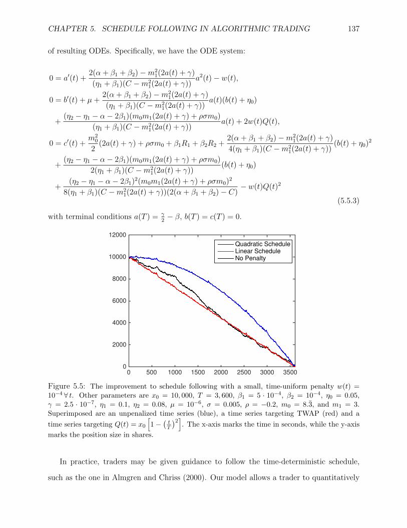
CHAPTER 5. SCHEDULE FOLLOWING IN ALGORITHMIC TRADING 137
of resulting ODEs. Specifically, we have the ODE system:
0 = a′(t) +2(α + β1 + β2)−m2
1(2a(t) + γ)
(η1 + β1)(C −m21(2a(t) + γ))
a2(t)− w(t),
0 = b′(t) + µ+2(α + β1 + β2)−m2
1(2a(t) + γ)
(η1 + β1)(C −m21(2a(t) + γ))
a(t)(b(t) + η0)
+(η2 − η1 − α− 2β1)(m0m1(2a(t) + γ) + ρσm0)
(η1 + β1)(C −m21(2a(t) + γ))
a(t) + 2w(t)Q(t),
0 = c′(t) +m2
0
2(2a(t) + γ) + ρσm0 + β1R1 + β2R2 +
2(α + β1 + β2)−m21(2a(t) + γ)
4(η1 + β1)(C −m21(2a(t) + γ))
(b(t) + η0)2
+(η2 − η1 − α− 2β1)(m0m1(2a(t) + γ) + ρσm0)
2(η1 + β1)(C −m21(2a(t) + γ))
(b(t) + η0)
+(η2 − η1 − α− 2β1)2(m0m1(2a(t) + γ) + ρσm0)2
8(η1 + β1)(C −m21(2a(t) + γ))(2(α + β1 + β2)− C)
− w(t)Q(t)2
(5.5.3)
with terminal conditions a(T ) = γ2− β, b(T ) = c(T ) = 0.
Time (seconds)0 500 1000 1500 2000 2500 3000 3500
Sh
are
s H
eld
0
2000
4000
6000
8000
10000
12000
Quadratic ScheduleLinear ScheduleNo Penalty
Figure 5.5: The improvement to schedule following with a small, time-uniform penalty w(t) =10−4 ∀ t. Other parameters are x0 = 10, 000, T = 3, 600, β1 = 5 · 10−4, β2 = 10−4, η0 = 0.05,γ = 2.5 · 10−7, η1 = 0.1, η2 = 0.08, µ = 10−6, σ = 0.005, ρ = −0.2, m0 = 8.3, and m1 = 3.Superimposed are an unpenalized time series (blue), a time series targeting TWAP (red) and a
time series targeting Q(t) = x0
[1−
(tT
)2]. The x-axis marks the time in seconds, while the y-axis
marks the position size in shares.
In practice, traders may be given guidance to follow the time-deterministic schedule,
such as the one in Almgren and Chriss (2000). Our model allows a trader to quantitatively

CHAPTER 5. SCHEDULE FOLLOWING IN ALGORITHMIC TRADING 138
evaluate the cost of deviating from schedule. Here, we illustrate the allocation of market
and limit orders over time accounting for the penalty of schedule deviation. Figure 5.5
displays the trader’s stock holdings over time in three settings: (i) a quadratic schedule
defined by Q(t) = x0
[1−
(tT
)2], and (ii) a linear schedule Q(t) = x0
(1− t
T
), and (iii) no
schedule (wherein we set w(t) ≡ 0). As we can see, the trader’s position persistently tracks
the schedule over the trading horizon, even with a small constant penalization coefficient
w(t) = 10−4. Compared to the linear schedule, the quadratic schedule is useful for an
institution that seeks to start out trading slowly and eventually speed up at the end of the
sell program. We see that our model is capable of handling complicated non-linear schedules
for stock holdings over time.
We examine the effects on trading rates in Figure 5.6. On the left panel, there is no
penalty for deviating from the linear schedule, while on the right we give a small penalty for
deviating. We find that the penalized allocator trades much more quickly and reacts more
quickly to price movements. Indeed, the non-penalized trading rates are very stable until
the very end of the sell program and the penalized trading rates change rapidly over time.
In contrast, the total trading rate in the non-penalized case (right panel) is fluctuating in
a relatively small range. In the penalized case, more market orders are used over time, but
the opposite is true when the penalty is removed.

CHAPTER 5. SCHEDULE FOLLOWING IN ALGORITHMIC TRADING 139
Time (seconds)0 500 1000 1500 2000 2500 3000 3500
Tra
din
g R
ate
s (
share
s/s
ec.)
0.5
1
1.5
2
2.5
3
TotalLimit OrdersMarket Orders
Time (seconds)0 500 1000 1500 2000 2500 3000 3500
Tra
din
g R
ate
s (
share
s/s
ec.)
-2
0
2
4
6
8
10
TotalMarket OrdersLimit Orders
Figure 5.6: Comparison of trading rates with (left) and without penalty (right). In the penalizedcase, we penalize deviations from a linear schedule with constant weight w(t) = 10−4. Otherparameters are x0 = 10, 000, T = 3, 600, β1 = 5 · 10−4, β2 = 10−4, η0 = 0.05, γ = 2.5 · 10−7,η1 = 0.1, η2 = 0.08, µ = 10−6, σ = 0.005, ρ = −0.2, m0 = 8.3, and m1 = 3. Final positions are190.4408 and 94.4218, respectively. The x-axis marks the time in seconds, while the y-axis marksthe trading rate in shares/sec.

Bibliography
Ahn, D. and Gao, B. (1999). A parametric nonlinear model of term structure dynamics. The
Review of Financial Studies, 12(4):721–762.
Alexander, C. and Barbosa, A. (2008). Hedging index exchange traded funds. Journal of Banking
and Finance, 32(2):326–337.
Alexander, C. and Korovilas, D. (2013). Volatility exchange-traded notes: Curse or cure? The
Journal of Alternative Investments, 16(2):52–70.
Almgren, R. and Chriss, N. (2000). Optimal execution of portfolio transactions. Journal of Risk,
3:5–39.
Avellaneda, M. and Stoikov, S. (2008). High-frequency trading in a limit order book. Quantitative
Finance, 8(3):217–224.
Avellaneda, M. and Zhang, S. (2010). Path-dependence of leveraged ETF returns. SIAM Journal
of Financial Mathematics, 1(2):586–603.
Bamberg, G. and Wagner, N. (2000). Equity index replication with standard and robust regression
estimators. OR Spektrum, 22(4):525–543.
Baur, D. G. (2012). Asymmetric volatility in the gold market. The Journal of Alternative Invest-
ments, 14(4):26–38.
Baur, D. G. (2013). Exchange-traded funds on gold - a free lunch? FIRN Research Paper.
Baur, D. G. and McDermott, T. K. (2010). Is gold a safe haven? International evidence. Journal
of Banking and Finance, 34(8):18861898.
140

BIBLIOGRAPHY 141
Bertsimas, D. and Lo, A. (1998). Optimal control of execution costs. Journal of Financial Markets,
1(1):1–50.
Black, F. (1976). Studies of stock price volatility changes. In Proceedings of the 1976 Meetings of
the American Statistical Association, Business and Economics Statistics Section, pages 177–181.
Black, F. and Scholes, M. (1973). The pricing of options and corporate liabilities. The Journel of
Political Economy, 81(3):637–654.
Bulthuis, B., Concha, J., Leung, T., and Ward, B. (2017a). Fast and precautious: Order controls
for trade execution. Risk Magazine, pages 84–89.
Bulthuis, B., Concha, J., Leung, T., and Ward, B. (2017b). Optimal execution of limit and market
orders with trade director, speed limiter, and fill uncertainty. Journal of Financial Engineering.
Cartea, A. and Jaimungal, S. (2015). Optimal execution with limit and market orders. Quantitative
Finance, 15(8):1279–1291.
Cartea, A. and Jaimungal, S. (2016). A closed-form execution strategy to target volume weighted
average price. SIAM Journal of Financial Mathematics, 7(1):760–785.
Cartea, A., Jaimungal, S., and Penalva, J. (2015). Algorithmic and High-Frequency Trading. Cam-
bridge University Press, 1st edition.
Cheng, M. and Madhavan, A. (2009). The dynamics of leveraged and inverse exchange-traded
funds. Journal of Investment Management, 7(4):43–62.
Cheng, X., Di Giacinto, M., and Wang, T. (2017). Optimal execution with uncertain order fills in
Almgren-Chriss framework. Quantitative Finance, 17(1):55–69.
Cox, J. C., Ingersoll, J. E., and Ross, S. A. (1985). A theory of the term structure of interest rates.
Econometrica, 53(2):385–408.
Deng, G., McCann, C., and Wang, O. (2012). Are VIX futures ETPs effective hedges? The Journal
of Index Investing, 3(3):35–48.

BIBLIOGRAPHY 142
Duffie, D. and Kan, R. (1996). A yield-factor model of interest rates. Mathematical Finance,
6(4):379–406.
Dunis, C. L., Laws, J., Middleton, P. W., and Karathanasopoulos, A. (2013). Nonlinear forecasting
of the gold miner spread: An application of correlation filters. Intelligent Systems in Accounting,
Finance and Management, 20(4):207–231.
Edirisinghe, N. C. P. (2013). Index-tracking optimal portfolio selection. Quantitative Finance
Letters, 1(1):16–20.
Feller, W. (1951). Two singular diffusion problems. The Annals of Mathematics, 54(1):173–182.
Ghosh, D., Levin, E. J., MacMillan, P., and Wright, R. E. (2004). Gold as an inflation hedge?
Studies in Economics and Finance, 22(1):1–25.
Grubichler, A. and Longstaff, F. (1996). Valuing futures and options on volatility. Journal of
Banking and Finance, 20(6):985–1001.
Guedj, I., Li, G., and McCann, C. (2011). Futures-based commodities ETFs. The Journal of Index
Investing, 2(1):14–24.
Guilbaud, F. and Pham, H. (2013). Optimal high-frequency trading with limit and market orders.
Quantitative Finance, 13(1):79–94.
Guo, K. and Leung, T. (2015). Understanding the tracking errors of commodity leveraged ETFs.
In Ludkovski, M., Sircar, R., and Aid, R., editors, Commodities, Energy, and Environmental
Finance, Fields Institute Communications, pages 39–63. Springer.
Guo, K. and Leung, T. (2017). Understanding the non-converge of agricultural futures via stochastic
storage costs and timing options. Journal of Commodity Markets.
Heston, S. L. (1993). A closed-form solution for options with stochastic volatility with applications
to bond and currency options. Review of Financial Studies, 6(2):327–343.

BIBLIOGRAPHY 143
Holzhauer, H., Lu, X., McLeod, R. W., and Mehran, J. (2013). Bad news bears: Effects of
expected market volatility on daily tracking error leveraged bull and bear ETFs. Managerial
Finance, 39(12):1169–1187.
Husson, T. and McCann, C. (2011). The VXX ETN and volatility exposure. PIABA Bar Journal,
18(2):235–252.
Ivanov, S. (2013). The influence of ETFs on the price discovery of gold, silver and oil. Journal of
Economics and Finance, 37(3):453–462.
Jarrow, R. (2010). Understanding the risks of leveraged ETFs. Finance Research Letters, 7(3):135–
139.
Kladivko, K. (2007). Maximum likelihood estimation of the Cox-Ingersoll-Ross process: the MAT-
LAB implementation. Technical Computing Prague.
Lee, K. (2008). Risk minimization under budget constraints. The Journal of Risk Finance, 9(1):71–
80.
Lehalle, C. and Laruelle, S. (2013). Market Microstructure in Practice. World Scientific Publishing
Company, 1st edition.
Leung, T., Li, J., Li, X., and Wang, Z. (2016a). Speculative futures trading under mean reversion.
Asia-Pacific Financial Markets, 23(4):281304.
Leung, T. and Li, X. (2015). Optimal mean reversion trading with transaction costs and stop-loss
exit. International Journal of Theoretical and Applied Finance, 18(3):1550020.
Leung, T. and Li, X. (2016). Optimal Mean Reversion Trading: Mathematical Analysis and Prac-
tical Applications. World Scientific, Singapore.
Leung, T., Lorig, M., and Pascucci, A. (2016b). Leveraged ETF implied volatilities from ETF
dynamics. Mathematical Finance.

BIBLIOGRAPHY 144
Leung, T. and Park, H. (2016). Long-term growth rate of expected utility for leveraged ETFs:
Martingale extraction approach. Working Paper. Available at https://ssrn.com/abstract=
2879976.
Leung, T. and Santoli, M. (2016). Leveraged Exchange-Traded Funds: Price Dynamics and Options
Valuation. Springer Briefs in Quantitative Finance, Springer.
Leung, T. and Sircar, R. (2015). Implied volatility of leveraged ETF options. Applied Mathematical
Finance, 22(2):162–188.
Leung, T. and Ward, B. (2015). The golden target: Analyzing the tracking performance of leveraged
gold ETFs. Studies in Economics and Finance, 32(3):278–297.
Leung, T. and Ward, B. (2017). Dynamic index tracking and risk exposure control using derivatives.
Working Paper. Available at https://ssrn.com/abstract=2976500.
Li, J. (2016). Trading VIX futures under mean reversion with regime switching. Journal of Financial
Engineering, 03(03):1650021.
Mencıa, J. and Sentana, E. (2013). Valuation of VIX derivatives. Journal of Financial Economics,
108(2):367–391.
Murphy, R. and Wright, C. (2010). An empirical investigation of the performance of commodity-
based leveraged ETFs. The Journal of Index Investing, 1(3):14–23.
Naylor, M., Wongchoti, U., and Gianotti, C. (2011). Abnormal returns in gold and silver exchange
traded funds. The Journal of Index Investing, 2(2):96–103.
Pavlova, I. and Daigler, R. T. (2008). The nonconvergence of vix futures at expiration. Review of
Futures Markets, 17(2):201–223.
Primbs, J. and Sung, C. (2008). A stochastic receding horizon control approach to constrained
index tracking. Asia-Pacific Financial Markets, 15(1):3–24.
Rompotis, G. G. (2011). Predictable patterns in ETFs’ return and tracking error. Studies in
Economics and Finance, 28(1):14–35.

BIBLIOGRAPHY 145
Smales, L. A. (2015). Asymmetric volatility response to news sentiment in gold futures. Journal
of International Financial Markets, Institutions & Money, 34:161–172.
Triantafyllopoulos, K. and Montana, G. (2011). Dynamic modeling of mean-reverting spreads for
statistical arbitrage. Computational Management Science, 8(1):23–49.
Uhlenbeck, G. E. and Ornstein, L. S. (1930). On the theory of the brownian motion. Physical
Review, 36(5):823–841.
Whaley, R. E. (2013). Trading volatility: At what cost? The Journal of Portfolio Management,
40(1):95–108.
Yao, D., Zhang, S., and Zhou, X. (2006). Tracking a financial benchmark using a few assets.
Operations Research, 54(2):232–246.

Appendix
In this Appendix, we provide a few proofs and derivations of the various formulas stated in
Chapter 4.
A.1 Derivation of SDE (4.1.5)
By Ito’s formula, the option price satisfies the SDE
dc(k)t =
∂c(k)
∂tdt+ dMᵀ
t ∇c(k) +1
2dMᵀ
t ∇2c(k)dMt. (A.1.1)
Here, the gradient and Hessian are taken with respect to all market variables, (S, Y (1), ..., Y (d)).
We rewrite the last term in (A.1.1) as follows:
dMᵀt ∇2c(k)dMt = (γtdt+ ΣtdB
Qt )ᵀ∇2c(k)(γtdt+ ΣtdB
Qt )
=(dBQ
t
)ᵀΣᵀt∇2c(k)ΣtdB
Qt
= Tr[(dBQ
t
)ᵀΣᵀt∇2c(k)ΣtdB
Qt
],
(A.1.2)
146

BIBLIOGRAPHY 147
where we have used the property that a scalar is equal to its own trace. Using that along
with the cyclic property of the trace, we have
dMᵀt ∇2c(k)dMt = Tr
[Σᵀt∇2c(k)ΣtdB
Qt
(dBQ
t
)ᵀ]= Tr
[Σᵀt∇2c(k)ΣtIdt
]= Tr
[Σᵀt∇2c(k)Σt
]dt. (A.1.3)
Substituting (A.1.3) into (A.1.1), we obtain
dc(k)t =
(∂c(k)
∂t+
1
2Tr[Σᵀt∇2c(k)Σt
])dt+
∂c(k)
∂SdSt +
∂c(k)
∂Y (1)dY
(1)t + ...+
∂c(k)
∂Y (d)dY
(d)t .
(A.1.4)
On the other hand, the Feynman-Kac formula tells us that the derivative price satisfies
∂c(k)
∂t+ γ
(0)t
∂c(k)
∂S+ γ
(1)t
∂c(k)
∂Y (1)+ ...+ γ
(d)t
∂c(k)
∂Y (d)+
1
2Tr[Σᵀt∇2c(k)Σt
]= rc(k), (A.1.5)
with the terminal condition: c(k)(Tk, s, y(1), ..., y(d)) = h(k)(s, y1, ..., yd) for all vectors (s, y1, ..., yd)
with strictly positive components. Using (A.1.4), we have
dc(k)t =
(rc
(k)t − γ
(0)t
∂c(k)
∂S− γ(1)
t
∂c(k)
∂Y (1)− ...− γ(d)
t
∂c(k)
∂Y (d)
)dt
+∂c(k)
∂SdSt +
∂c(k)
∂Y (1)dY
(1)t + ...+
∂c(k)
∂Y (d)dY
(d)t .
Dividing both sides by c(k)t and using the definitions listed in (4.1.6), we obtain SDE (4.1.5).
A.2 Validation of (4.3.10) when Mean-Reversion Speeds
are Equal
We now demonstrate that, in the special case of κ = γ under the CSQR model, tracking
strategies exist using two futures on S of different maturities. The elasticity with respect
to the index is the same as in (4.3.9); however, the elasticity with respect to the stochastic

BIBLIOGRAPHY 148
mean is
H(k)t =
Yt
fTkt
∂fTkt∂Y
=Yt
fTktγeκt−γTk(Tk − t). (A.2.1)
Substituting (A.2.1) into (4.3.10), we have
St
fT1t
e−γ(T1−t) Yt
fT2t
γeκt−γT2(T2 − t) 6=St
fT2t
e−γ(T2−t) Yt
fT1t
γeκt−γT1(T1 − t)
⇐⇒ e−γ(T1−t)eκt−γT2(T2 − t) 6= e−γ(T2−t)eκt−γT1(T1 − t) ⇐⇒ T1 6= T2.
Under the assumption that T1 < T2, the resulting system is solvable and yields strategies
that achieve the given exposures.
A.3 Solution to (4.3.11) when Mean-Reversion Speeds
are Equal
With the elasticity with respect to the stochastic mean given by (A.2.1) and κ = γ under
the CSQR model, the portfolio weights that solve system (4.3.11) are
u(1)t =
βfT1t
St
(eγ(T1−t)(T2 − t)
T2 − T1
)− ηfT1
t
Yt
(eγ(T1−t)
γ(T2 − T1)
),
and
u(2)t =
−βfT2t
St
(eγ(T2−t)(T1 − t)
T2 − T1
)+ηfT2
t
Yt
(eγ(T2−t)
γ(T2 − T1)
).
In particular, take β = 1 and η = 0. Then, the portfolio weights simplify to
u(1)t =
fT1t
St
(eγ(T1−t)(T2 − t)
T2 − T1
), and u
(2)t =
−fT2t
St
(eγ(T2−t)(T1 − t)
T2 − T1
).
By inspection, u(1)t is positive while u
(2)t is negative.

BIBLIOGRAPHY 149
A.4 Validation of (4.3.10) when Mean-Reversion Speeds
are Unequal
We substitute the elasticities from (4.3.9) into (4.3.10), and then check directly whether or
not the following holds:
St
fT1t
e−γ(T1−t) Yt
fT2t
γ
γ − κ(e−κ(T2−t) − e−γ(T2−t)
)6= St
fT2t
e−γ(T2−t) Yt
fT1t
γ
γ − κ(e−κ(T1−t) − e−γ(T1−t)
)⇐⇒ e−γT1
(e−κ(T2−t) − e−γ(T2−t)
)6= e−γT2
(e−κ(T1−t) − e−γ(T1−t)
)⇐⇒ T1 6= T2.
Since we assume T1 < T2, the resulting system is solvable and allows for strategies to attain
the required exposures.