optimal designs for some selected nonlinear...

Contents lists available at ScienceDirect

Journal of Statistical Planning and Inference

Journal of Statistical Planning and Inference 154 (2014) 102–115

http://d0378-37

n CorrE-m1 Re2 Re

journal homepage: www.elsevier.com/locate/jspi

Optimal designs for some selected nonlinear models

A.S. Hedayat n,1, Ying Zhou 1, Min Yang 2

Department of Mathematics, Statistics, and Computer Science, University of Illinois at Chicago, Science and Engineering Offices (M/C 249),851 S. Morgan Street, Chicago, IL 60607-7045, United States

a r t i c l e i n f o

Article history:Received 18 September 2013Received in revised form6 May 2014Accepted 6 May 2014Available online 22 May 2014

Keywords:Support pointsAdaptive designsLocally optimal designs

x.doi.org/10.1016/j.jspi.2014.05.00558/& 2014 Elsevier B.V. All rights reserved.

esponding author.ail addresses: [email protected] (A.S. Hedayatsearch is supported by the U.S. National Scisearch is supported by the U.S. National Sci

a b s t r a c t

Some design aspects related to three complex nonlinear models are studied in this paper.For Klimpel's flotation recovery model, it is proved that regardless of model parameterand optimality criterion, any optimal design can be based on two design points and theright boundary is always a design point. For this model, an analytical solution for aD-optimal design is derived. For the 2-parameter chemical kinetics model, it is found thatthe locally D-optimal design is a saturated design. Under a certain situation, any optimaldesign under this model can be based on two design points. For the 2n-parametercompartment model, compared to the upper bound by Carathe ́odory's theorem, the upperbound of the maximal support size is significantly reduced by the analysis of relatedTchebycheff systems. Some numerically calculated A-optimal designs for both Klimpel'sflotation recovery model and 2-parameter chemical kinetic model are presented. For eachof the three models discussed, the D-efficiency when the parameter misspecificationhappens is investigated. Based on two real examples from the mining industry, it isdemonstrated how the estimation precision can be improved if optimal designs would beadopted. A simulation study is conducted to investigate the efficiencies of adaptivedesigns.

& 2014 Elsevier B.V. All rights reserved.

1. Introduction

Optimal designs based on nonlinear models have wide and important applications in many areas of science. A goodexample of the application is the optimal design based on PK/PD models which are widely used in pharmaceutical industriesfor the examination of absorption, distribution, metabolism, elimination, efficacy and toxicity parameters in drugdevelopments, see Gieschke and Steimer (2000) and Meibohm and Derendorf (2002).

We study and explore optimal designs for three complex nonlinear models. These are the 2-parameter chemical kineticmodel, the 2n-parameter compartment model and the 2-parameter Klimpel's flotation recovery model. These three modelshave been shown to have extensive applications in real life situations (Godfrey, 1983; Jacquez, 1985; Parekh and Miller, 1999;Saleh, 2010; Yuan et al., 1996).

We concentrate on the nonlinear model y¼ ηðx; θÞþε, where θ¼ ðθ1; θ2;…; θkÞT is a vector of k unknown parameters and xis the explanatory variable defined on a design space χ in R. The error ε is postulated to be distributed as Nð0; s2Þ andwithout loss of generality we let s¼ 1. Further, we assume that all observations are independent.

), [email protected] (Y. Zhou), [email protected] (M. Yang).ence Foundation Grants DMS-0904125 and DMS-1306394.ence Foundation Grants DMS-0707013 and DMS-1322797.

www.sciencedirect.com/science/journal/03783758

www.elsevier.com/locate/jspi

http://dx.doi.org/10.1016/j.jspi.2014.05.005



http://crossmark.crossref.org/dialog/?doi=10.1016/j.jspi.2014.05.005&domain=pdf



mailto:[email protected]




A.S. Hedayat et al. / Journal of Statistical Planning and Inference 154 (2014) 102–115 103

Typically, the optimal nonlinear design studies are under approximate theory, i.e., instead of exact sample sizes fordesign points, design weights are used. Let ξ be any n-point approximate design,

ξ¼t1 t2 …tnω1 ω2 …ωn

!:

Here 0oωio1 represents the proportion of the number of points studied at ti with ∑ni ¼ 1ωi ¼ 1. The Fisher information

matrix for y¼ ηðt; θÞþε can be written as

Iξ ¼ ∑n

i ¼ 1ωi

∂ηðt; θÞ∂θ

� �∂ηðt; θÞ∂θ

� �T

: ð1:1Þ

How to compare two designs? There are variety of optimality criteria. Two popular optimality criteria are D-optimality andA-optimality, which are to maximize jIξj and minimize TrðI�1

ξ Þ over all possible designs, respectively. A D-optimal designminimizes the volume of an asymptotic confidence ellipsoid for θ, and an A-optimal design minimizes the average of theasymptotic variances for the estimators of the individual parameters.

2. Preliminaries

In this paper, we shall use and deal with Extended Tchebycheff systems and Extended Complete Tchebysheff systems.The Tchebycheff systems were first introduced by the Russian mathematicians Chebyshev (1859) and Bernshtein (1937).In Karlin and Studden (1966), the theory of the Tchebycheff systems and its applicability in optimal design of experimentstheory is introduced and studied.

Let fu0;u1;…;ung be nþ1 continuous real-valued functions on ½a; b�. fugnk ¼ 0 ¼ fu0;u1;…;ung is called a Tchebycheff system(T-system) if the following determinant is strictly positive whenever art0ot1o⋯otnrb

U0; 1; …; n

t0; t1; …; tn

!¼

u0ðt0Þ u0ðt1Þ ⋯ u0ðtnÞu1ðt0Þ u1ðt1Þ ⋯ u1ðtnÞ

⋮ ⋮ ⋮ ⋮unðt0Þ unðt1Þ ⋯ unðtnÞ

��

��40:

fugnk ¼ 0 is called a Complete Tchebycheff system (CT-system) if fugmk ¼ 0 is a T-system on ½a; b� for eachm¼ 0;1;…;n. In the sequel,we shall deal with Extended Tchebycheff system and Extended Complete Tchebysheff system, which are defined below:

(i)
fugnk ¼ 0 on ½a; b� is called an Extended Tchebycheff system (ET-system) of order p, provided uiACp�1½a; b�, i¼ 0;1;…;nand
Un0; 1; …; n

t0; t1; …; tn

!40

for all choices art0rt1r⋯rtnrb, where equality occurs in groups of at most p consecutive ti values. Here,

Un0; 1; …; nt0; t1; …; tn

!

has the same definition as

U0; 1; …; n

t0; t1; …; tn

!

except that, for each set of equality ti, we replace successive columns by their successive derivatives. For example,suppose art0 ¼ t1 ¼⋯¼ tqotqþ1o⋯otn�1 ¼ tnrb then

Un0; 1; …; n

t0; t1; …; tn

!¼

u0ðt0Þ uð1Þ0 ðt0Þ ⋯ uðqÞ

0 ðt0Þ u0ðtqþ1Þ ⋯ u0ðtn�1Þ uð1Þ0 ðtn�1Þ

u1ðt0Þ uð1Þ1 ðt0Þ ⋯ uðqÞ

1 ðt0Þ u1ðtqþ1Þ ⋯ u1ðtn�1Þ uð1Þ1 ðtn�1Þ

⋮ ⋮ ⋯ ⋮ ⋮ ⋯ ⋮ ⋮unðt0Þ uð1Þ

n ðt0Þ ⋯ uðqÞn ðt0Þ unðtqþ1Þ ⋯ unðtn�1Þ uð1Þ

n ðtn�1Þ

��

��:

In the above, uðjÞk ðtÞ denotes the jth order derivative of uk.

(ii)
fugnk ¼ 0 is called an Extended Complete Tchebysheff system (ECT-system) if fugmk ¼ 0 is an ET-system on ½a; b� for eachm¼ 0;1;…;n. The following results are known and we skip the proofs.
(a)
fugnk ¼ 0 on ½a;b� is a Tchebysheff system if and only if every non-trivial linear combination gðtÞ ¼∑ni ¼ 0ciuiðtÞ has at most n
zeros, where ðc0; c1;…; cnÞa ð0;0;…;0Þ.

A.S. Hedayat et al. / Journal of Statistical Planning and Inference 154 (2014) 102–115104

(b)
fugnk ¼ 0 on ½a;b� is an ECT-system if and only if for k¼ 0;1;…;n,
Wðu0;u1;…;ukÞðtÞ ¼

u0ðtÞ uð1Þ0 ðtÞ ⋯ uðkÞ

0 ðtÞu1ðtÞ uð1Þ

1 ðtÞ ⋯ uðkÞ1 ðtÞ

⋮ ⋮ ⋮ ⋮ukðtÞ uð1Þ

k ðtÞ ⋯ uðkÞk ðtÞ

��

��40

where Wðu0;u1;…;ukÞðtÞ is the Wronskian determinant, see Hartman (1964).

3. Klimpel's flotation recovery model

Flotation model is a gravity separation process that originated from processing of minerals. They are widely used inmining engineering and have found wide application in industrial waste-water treatment. It is also useful in theconcentration of a variety of dissolved chemical species often following a sorption process. They are based on anobservation that was made in the earliest experimental kinetic studies of flotation, namely, that not all particles will berecovered by flotation no matter how much time they have in the flotation environment. Each particle type has an ultimaterecovery that is less than 100 percent. The particles that do float are recovered at a rate that is governed by a simple first-order kinetic law. Thus two kinetic parameters are required for each type of particle: the ultimate recovery and the kineticconstant. There are three types of flotation recovery models: exponential flotation recovery model, Klimpel's flotationrecovery model and Agar's flotation recovery model. We will discuss and treat Klimpel's flotation recovery model.

The 2-parameter Klimpel's flotation recovery model is widely used in environmental science for metal recovery:

R t;Rmax; kð Þ ¼ Rmax 1� 1kt

1�e�kt� ��

þε: ð3:1Þ

Rðt;Rmax; kÞ refers to the recovery of mineral or metal of interest; t refers to time and Rmax is the ultimate recovery while kis constant first-order rate.

For an easy presentation, we rewrite Model (3.1) in the following form:

y¼ η t; θð Þþε¼ a 1� 1bt

1�e�bt� ��

þε ð3:2Þ

where θ¼ ða; bÞ0.

Theorem 3.1. Under Model (3.2), for any arbitrary design ξ, there exists a design ξn such that IξðθÞr Iξn ðθÞ (here and elsewhere,matrix inequalities are under the Loewner ordering). Here, ξn is based on two design points including the upper bound point T ofthe design space. When IξðθÞr Iξn ðθÞ, it means design ξn is not inferior to ξ under commonly used matrix based optimality criteria.An optimal design under Loewner ordering criterion does not exist in general. We have to consider optimal design under lessrestrictive criteria.

Proof. For any arbitrary design ξ¼ ðti;ωiÞ, i¼ 1;…;n, it can be shown that the Fisher information matrix Iξ can be written inthe form:

Iξ ¼ PðθÞCðξ; θÞPðθÞT : ð3:3ÞHere

P θð Þ ¼1 0�a

bab

!and C ξ; θð Þ ¼ ∑

n

i ¼ 1ωi

ð1þ xilnð1� xiÞÞ

2 xi 1þ xilnð1�xiÞ

� �xi 1þ xi

lnð1� xiÞ

� �x2i

0B@

1CA;

with xi ¼ 1�e�bti . Since 0otrT , we have 0oxio1�e�bT .Let Ψ1ðxÞ ¼ x2, Ψ2ðxÞ ¼ xð1þx=lnð1�xÞÞ, and Ψ3ðxÞ ¼ ð1þx=lnð1�xÞÞ2. We can verify that for any 0oxo1,

(a)
Ψ 01ðxÞ40;
(b)
ðΨ 02ðxÞ=Ψ 0
1ðxÞÞ040;
(c) ððΨ 0
3ðxÞ=Ψ 01ðxÞÞ0=ðΨ 0

2ðxÞ=Ψ 01ðxÞÞ0Þ040;

(d)
limx↑ð1� e� bT ÞðΨ 02ðxÞ=Ψ 0
1ðxÞÞðΨ1ð1�e�bT Þ�Ψ1ðxÞÞ ¼ 0.

The above inequalities are rather difficult to verify by hand since involving manipulation of derivative, therefore we usesymbolic computational software MAPLE(Waterloo, Canada) to verify them. By Corollary 3 of Yang and Stufken (2009), thereexists a design with two design points including the upper bound T, say ξn, such that one diagonal element and the off-diagonal element of Cðξn; θÞ are the same as that of Cðξ; θÞ, and the remaining diagonal element is larger. Thus the conclusionfollows. □

Table 1xn for the D-optimal design for θ under Model (3.2).

b 0.2 0.4 0.6 0.8 1.0 1.2 1.4 1.6

xn 8.3817 4.3395 2.9253 2.2060 1.7705 1.4786 1.2693 1.1119

Table 2ðxn;ωnÞ for the A-optimal design for θ under Model (3.2).

b 0.2 0.4 0.6 0.8

ðxn;ωnÞ (7.1165, 0.3903) (3.6294, 0.5283) (2.3780, 0.5929) (1.7594, 0.6261)

b 1.0 1.2 1.4 1.6

ðxn;ωnÞ (1.3951, 0.6449) (1.1558, 0.6563) (0.9869, 0.6638) (0.8612, 0.6689)


Theorem 3.1 shows that no matter what optimal designs we are looking for, we can always restrict ourself to two-pointsdesign including the upper bound T, irrespective of parameters of interest or the optimality criterion. Consequently, we areable to obtain analytical expression for some specific optimal designs.

Corollary 3.1. Under Model (3.2), ξn is the D-optimal design for θ, where ξn ¼ fðT ;0:5Þ; ðtn;0:5Þg, where tn ¼ � lnð1�xnÞ=b andxn is the unique solution of the following equation:

1�e�bT� � ln 1�xð Þþ x

1�xln2ð1�xÞ

0B@

1CA� 1� 1

bT1�e�bT� ��

¼ 0:

Proof. By Theorem 3.1, a D-optimal design, which maximizes determinant of Iξ, for θ must only have two design pointsincluding the upper bound T. Consequently, it must have equal weights on each support point (Silvey, 1980). Thus aD-optimal design for θ must maximize g2ðxÞ, where

g xð Þ ¼ 1�e�bT� �

1þ xlnð1�xÞ

� ��x 1� 1


:

Clearly gðxÞ ¼ 0 when x¼ 1�e�bT . We can show that limx↓0gðxÞ ¼ 0. Now let us consider the first derivative of g(x),

g0 xð Þ ¼ 1�e�bT� � ln 1�xð Þþ x

1�xln2ð1�xÞ

0B@

1CA� 1� 1


:

With some simple algebra, we can show that (i) g0ðxÞ is a strictly increasing function on ð0;1Þ; (ii) limx↓0g0ðxÞo0 and(iii) g0ðxÞ40 when x¼ 1�e�bT . Thus, there must exist a unique solution xn such that g0ðxnÞ ¼ 0, g0ðxÞo0 when 0oxoxn,and g0ðxÞ40 when xnoxr1�e�bT . So g(x) is minimized at x¼ xn. Combining the fact the gðxÞ ¼ 0 when x¼ 1�e�bT andlimx↓0gðxÞ ¼ 0, g2ðxÞ must be maximized at xn. □

From Theorem 3.1, we notice that the D-optimal design does not depend on parameter a. Once the values of upper boundT and the parameter b are given, the value of xn can be easily computed. For example, when T¼100, Table 1 provides thevalue of xn for some selected b values.

Although it may not be easy to derive other optimal designs, we may be able to derive any optimal design numericallydue to the simple format of ξn in Theorem 3.1. For example, let us consider A-optimal designs for θ, which minimizes thetrace of I�1

ξ . With the explicit optimal weight formula provided by Biedermann et al. (2006), the numerical search turns outto be one dimension which can be easily carried out. Table 2 provides the optimal designs for T¼100, a¼1 under someselected b values.

4. 2-Parameter chemical kinetic model

Kinetic models related to chemical reactions are widely used in chemical engineering and chemistry. The models areusually in the form of differential equations with two groups of parameters, the rate and the order of reaction; seeBoroujerdi (2001).


Consider the consecutive reaction: A⟶B, with reaction order λ and reaction rate θ. The kinetic model is given by thedifferential equation:

d½A�dt

¼ �θ½A�λ; ð4:1Þ

where tZ0 is the reaction time, λ40 is the reaction order, θ40 is the reaction rate.Given (4.1), with the initial conditions A¼1, B¼0 at t¼0, the model is determined as follows:

½A� ¼ ηðt; θ; λÞþε¼ ½1�ð1�λÞθt�1=ð1� λÞ þε: ð4:2Þ

Theorem 4.1. Under Model (4.2), a D-optimal design for all parameters is supported on two points.

Proof. By the extended equivalence theorem of Kiefer (1974) established by White (1973), it is enough to verify that thereare at most 2 maximal points for dðξ; x; θÞ, directional derivative, which will be introduced shortly.Let 1=ð1�λÞ ¼ β, 1�ðθ=βÞt ¼ x, and θ0 ¼ ðθ; βÞ. Note that a D-optimal design for λ and θ is the same as that for β and θ. The

Fisher information matrix for ξ is

Iξ ¼1θ2∑n

i ¼ 1ωiβ2x2β�2

i ðxi�1Þ2 1θ∑

ni ¼ 1ωiβx

2β�1i xi�1ð Þ ln xiþ 1

xi�1

� �1θ∑

ni ¼ 1ωiβx

2β�1i xi�1ð Þ ln xiþ 1

xi�1

� �∑n

i ¼ 1ωiðln xiþ 1xi�1Þ2x2βi

0B@

1CA:

We tacitly assume that nZ2 and that xi's are all distinct. This ensures the existence of the inverse of the Fisher informationmatrix,

I�1ξ ¼

m11 m12

m21 m22

!

with m12 ¼m21.Then,

d ξ; x; θð Þ ¼ tr1θ2β2x2β�2ðx�1Þ2 β

θx2β�1 x�1ð Þ ln xþ1

x�1

βθx

2β�1 x�1ð Þ ln xþ1x�1

ðln xþ1x�1Þ2x2β

0@

1A m11 m12

m21 m22

!

¼m11

θ2β2x2β�2ðx�1Þ2þ2

θm12βx2β�1 x�1ð Þ ln xþ1

x�1

� �þm22x2β ln xþ1

x�1

� �2

:

We obtain the first order derivative of dðξ; x; θÞ with respect to x, which is denoted by d0ðξ; x; θÞ:

d0ðξ; x; θÞ ¼ x2β�3fk1x2þk2xþk3þk4x2ln xþk5x2ðln xÞ2þk6x ln xg ð4:3Þwhere k1 ¼ 2ð1=θ2Þm11β

3�4ð1=θÞm12β2þ2ð1=θÞm12βþ2m22β�2m22, k2 ¼ �4ð1=θ2Þm11β

3þ2ð1=θ2Þm11β2þ8ð1=θÞm12β

2�6ð1=θÞm12β�4m22βþ4m22, k3 ¼ 2ð1=θ2Þm11β

3�2ð1=θ2Þm11β2�4ð1=θÞm12β

2þ4ð1=θÞm12βþ2m22β�2m22, k4 ¼ 4ð1=θÞ m12β2

�4m22βþ 2m22, k5 ¼ 2m22β, k6 ¼ �4ð1=θÞm12β2þ2ð1=θÞm12βþ4m22β�2m22 ¼ 2ð1�2βÞððβ=θÞm12�m22Þ.

We notice that d0ðξ; x; θÞ is composed of two Tchebycheff systems (Lemma 1 of Appendix) as indicated below:T1 ¼ f1; x; x2; x2 ln x; x2ðln xÞ2g and T2 ¼ f1; x; x2; x2 ln x; x ln xg.We consider two circumstances for β in studying

β

θm12�m22

� �¼ 1θ2

1jIξj

∑n

i ¼ 1β2ωix

2β�2i 1�xið Þxi ln xi: ð4:4Þ

Recall that β ð ¼ 1=ð1�λÞÞ is either greater than 1 or smaller than 0. Consequently ððβ=θÞm12�m22Þ is less than 0 for allfeasible values of β. Therefore k5 is positive for β41 and negative for βo0 while k6 is positive when β41 and negativewhen βo0.Since both T1 and T2 are T-systems with positive determinant, any positive linear combination of the two systems is also a

T-system.For β41, f1; x; x2; x2 ln x; k5x2ðln xÞ2þk6x lnj; xg is also a T-system with k540; k640.For βo0, f1; x; x2; x2 ln x; �½k5x2ðln xÞ2þk6x ln x�g is also a T-system with �k540; �k640.For both cases, there are at most 4 roots for d0ðξ; x; θÞ ¼ 0. Thus there are at most two local maximal points in ð0; TÞ. On the

other hand, for β41, when t-0, dðξ; x; θÞ-0; t-T , dðξ; x; θÞ-0, T is the upper bound. And for βo0, when t-0,dðξ; x; θÞ-0; t-T , dðξ; x; θÞ-0. Consequently, the two boundary points cannot be the support points. Thus, a D-optimaldesign is precisely supported on 2 points. □

When 0oλo1, we are able to extend our result to any arbitrary optimal design. To make Model (4.2) meaningful,1�ð1�λÞθt needs to be positive, i.e., 0oto ð1=ð1�λÞÞθ.

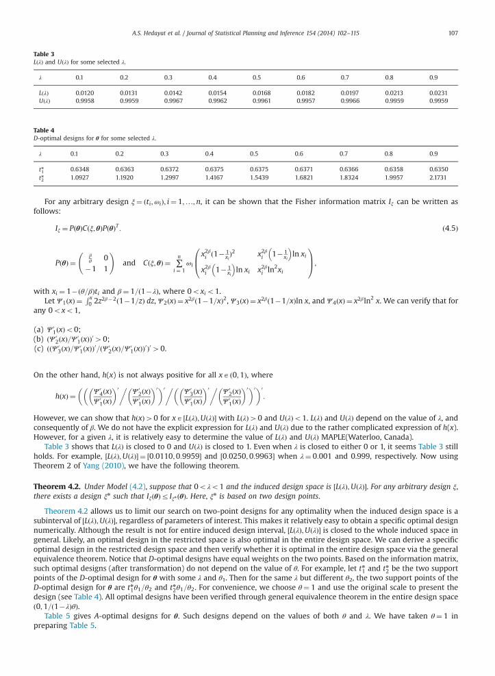
Table 3LðλÞ and UðλÞ for some selected λ.

λ 0.1 0.2 0.3 0.4 0.5 0.6 0.7 0.8 0.9

LðλÞ 0.0120 0.0131 0.0142 0.0154 0.0168 0.0182 0.0197 0.0213 0.0231UðλÞ 0.9958 0.9959 0.9967 0.9962 0.9961 0.9957 0.9966 0.9959 0.9959

Table 4D-optimal designs for θ for some selected λ.

λ 0.1 0.2 0.3 0.4 0.5 0.6 0.7 0.8 0.9

tn1 0.6348 0.6363 0.6372 0.6375 0.6375 0.6371 0.6366 0.6358 0.6350tn2 1.0927 1.1920 1.2997 1.4167 1.5439 1.6821 1.8324 1.9957 2.1731


For any arbitrary design ξ¼ ðti;ωiÞ; i¼ 1;…;n, it can be shown that the Fisher information matrix Iξ can be written asfollows:

Iξ ¼ PðθÞCðξ; θÞPðθÞT : ð4:5Þ

P θð Þ ¼βθ 0

�1 1

!and C ξ; θð Þ ¼ ∑

n

i ¼ 1ωi

x2βi ð1� 1xiÞ2 x2βi 1� 1

xi

� �ln xi

x2βi 1� 1xi

� �ln xi x2βi ln2xi

0B@

1CA;

with xi ¼ 1�ðθ=βÞti and β¼ 1=ð1�λÞ, where 0oxio1.Let Ψ1ðxÞ ¼

R x0 2z2β�2ð1�1=zÞ dz, Ψ2ðxÞ ¼ x2βð1�1=xÞ2, Ψ3ðxÞ ¼ x2βð1�1=xÞln x, and Ψ4ðxÞ ¼ x2βln2 x. We can verify that for

any 0oxo1,

(a)
Ψ 01ðxÞo0;
(b)
ðΨ 02ðxÞ=Ψ 0
1ðxÞÞ040;
(c) ððΨ 0
3ðxÞ=Ψ 01ðxÞÞ0=ðΨ 0

2ðxÞ=Ψ 01ðxÞÞ0Þ040.

On the other hand, h(x) is not always positive for all xAð0;1Þ, where

h xð Þ ¼ Ψ 04ðxÞ

Ψ 01ðxÞ

� �0 Ψ 02ðxÞ

Ψ 01ðxÞ

� �0�0 Ψ 03ðxÞ

Ψ 01ðxÞ

� �0 Ψ 02ðxÞ

Ψ 01ðxÞ

� �0�0�0:

��

However, we can show that hðxÞ40 for xA ½LðλÞ;UðλÞ� with LðλÞ40 and UðλÞo1. LðλÞ and UðλÞ depend on the value of λ, andconsequently of β. We do not have the explicit expression for LðλÞ and UðλÞ due to the rather complicated expression of h(x).However, for a given λ, it is relatively easy to determine the value of LðλÞ and UðλÞ MAPLE(Waterloo, Canada).

Table 3 shows that LðλÞ is closed to 0 and UðλÞ is closed to 1. Even when λ is closed to either 0 or 1, it seems Table 3 stillholds. For example, ½LðλÞ;UðλÞ� ¼ ½0:0110;0:9959� and ½0:0250;0:9963� when λ¼ 0:001 and 0.999, respectively. Now usingTheorem 2 of Yang (2010), we have the following theorem.

Theorem 4.2. Under Model (4.2), suppose that 0oλo1 and the induced design space is ½LðλÞ;UðλÞ�. For any arbitrary design ξ,there exists a design ξn such that IξðθÞr Iξn ðθÞ. Here, ξn is based on two design points.

Theorem 4.2 allows us to limit our search on two-point designs for any optimality when the induced design space is asubinterval of ½LðλÞ;UðλÞ�, regardless of parameters of interest. This makes it relatively easy to obtain a specific optimal designnumerically. Although the result is not for entire induced design interval, ½LðλÞ;UðλÞ� is closed to the whole induced space ingeneral. Likely, an optimal design in the restricted space is also optimal in the entire design space. We can derive a specificoptimal design in the restricted design space and then verify whether it is optimal in the entire design space via the generalequivalence theorem. Notice that D-optimal designs have equal weights on the two points. Based on the information matrix,such optimal designs (after transformation) do not depend on the value of θ. For example, let tn1 and tn2 be the two supportpoints of the D-optimal design for θ with some λ and θ1. Then for the same λ but different θ2, the two support points of theD-optimal design for θ are tn1θ1=θ2 and tn2θ1=θ2. For convenience, we choose θ¼ 1 and use the original scale to present thedesign (see Table 4). All optimal designs have been verified through general equivalence theorem in the entire design spaceð0;1=ð1�λÞθÞ.

Table 5 gives A-optimal designs for θ. Such designs depend on the values of both θ and λ. We have taken θ¼ 1 inpreparing Table 5.

Table 5A-optimal designs for θ for some selected λ.

λ 0.1 0.2 0.3 0.4

ðtn1 ;ωn

1Þ (0.5295, 0.6265) (0.5200, 0.5661) (0.5108, 0.5162) (0.5018, 0.4748)ðtn2 ;ωn

2Þ (1.1020, 0.3735) (1.2171, 0.4339) (1.3474, 0.4838) (1.4952, 0.5252)

λ 0.5 0.6 0.7 0.8

ðtn1 ;ωn

1Þ (0.4932, 0.4417) (0.4856, 0.4159) (0.4789, 0.3963) (0.4731, 0.3813)ðtn2 ;ωn

2Þ (1.6623, 0.5583) (1.8509, 0.5841) (2.0626, 0.6037) (2.2998, 0.6187)


5. 2n-Parameter compartment models

Compartment models are important for the evaluation of efficacy and toxicity in drug developments. There is substantialliterature investigating the nature of locally D-optimal designs for such models, see for example, Li and Majumdar (2008)and Fang and Hedayat (2008) from both theoretical and applied perspectives.

2n-Parameter compartment models are the sum of n open one-compartment model with zero-order input and first-order output. The process is described as follows. Drug is introduced into the compartment by a constant zero-order input,with rate of input k0; then the drug is eliminated from the compartment by the first-order elimination rate, with rate ofoutput KA. At the start, the amount of drug is low and gradually the amount increases and the rate of elimination increasesaccordingly, and eventually the rate of input and the rate of output are equal. Therefore, the amount or concentration ofdrug remains constant. The following differential equation defines the rate of accumulation of drug in the compartmentduring a single infusion with constant rate:

dAdt

¼ k0�KA: ð5:1Þ

Given the initial amount of the drug: Aðt ¼ 0Þ ¼ 0, we obtain integrated form:

A¼ k0K

1�e�Kt : ð5:2Þ

Compartment models are also extremely useful in modeling HIV dynamics, especially those multiple compartmentmodels with large numbers of parameters. In modeling HIV dynamics within a host, biomathematicians and theoreticalbiologists have made great advances in the development of mathematical models to study the characteristics of HIVreplication and HIV evolution. Most of these models are differential equations or compartmental models. See, for example,Ding and Wu (2000) and Han and Chaloner (2003). Here we start with 4-parameter compartment model (5.3).

Carathe0odory's theorem provides an upper bound for any k-parameter D-optimal design formulation. From the above

discussion of chemical kinetic model, we know d0ðξ; t; θÞ is very important in studying the numbers of support points. Herewe also follow the same idea and study the upper bounds of the number of support points for compartment models.

y¼ ηðt; θÞþε¼ a1ð1�e� λ1tÞþa2ð1�e� λ2tÞþε; ð5:3Þwhere 0rt, λ1; λ240, a1; a2AR, θ0 ¼ ða1; a2; λ1; λ2Þ.

Theorem 5.1. Under Model (5.3), the minimum upper bound of the number of support points for a locally D-optimal design is 6.

Proof. After simplification, we obtain

d0ðξ; t; θÞ ¼ e�2λ1t ½�2λ1m33t2þð2m33þ4λ1m13Þt�ð2m13þ2λ1m11Þ�þe�2λ2t ½�2λ2m44t2

þð2m44þ4λ2m24Þt�ð2m24þ2λ2m22Þ�þe�ðλ1 þ λ2Þt ½�2ðλ1þλ2Þm34t2þf4m34

þðλ1þλ2Þð2m24þ2m23Þgt�f2m14þ2m23þ2ðλ1þλ2Þm12g�þe� λ1t ½�λ1ð2m13

þ2m33Þtþf2m13þ2m33þλ1ð2m11þ2m12Þg�þe� λ2t ½�λ2ð2m14

þ2m24Þtþf2m14þ2m24þλ2ð2m22þ2m12Þg�:We follow the same idea of the approach used in Fang and Hedayat (2008) to obtain the upper bound of the number of

support points. We need to know the upper bounds for the numbers of roots for d0ðξ; t; θÞ ¼ 0. We will simplify d0ðξ; t; θÞ bytaking derivative several times and what we obtain after the last derivative step is a linear combination of a T-system. Basedon this, then we revisit the problem to determine bounds on the number of roots for d0ðξ; t; θÞ ¼ 0.

(1)
Divide both sides by e� λ1t and take derivative twice. (2) Divide both sides by eðλ1 � λ2Þt and take derivative twice. (3) Divide both sides by e� λ1t and take derivative three times.

Table 6D-efficiency when b40 deviates from the true value for a¼ 89%.

b Locally D-optimal design points D-efficiency (%)

0.02 tn1 ¼ 38:31; tn2 ¼ 100:00 62.550.04 tn1 ¼ 29:31; tn2 ¼ 100:00 80.570.06 tn1 ¼ 22:91; tn2 ¼ 100:00 92.670.08 tn1 ¼ 18:61; tn2 ¼ 100:00 98.440.1 tn1 ¼ 15:51; tn2 ¼ 100:00 1000.20 tn1 ¼ 8:41; tn2 ¼ 100:00 86.590.4 tn1 ¼ 4:31; tn2 ¼ 100:00 58.700.6 tn1 ¼ 2:91; tn2 ¼ 100:00 43.680.8 tn1 ¼ 2:21; tn2 ¼ 100:00 34.841.0 tn1 ¼ 1:81; tn2 ¼ 100:00 29.331.8 tn1 ¼ 1:01; tn2 ¼ 100:00 17.312.4 tn1 ¼ 0:71; tn2 ¼ 100:00 12.41


Then solving d0ðξ; t; θÞ ¼ 0 is equivalent to solving g1ðtÞ, where

g1ðtÞ ¼ λ21ðλ2�2λ1Þ2ðλ2�λ1Þ3eðλ2 � λ1Þt ½�2λ1m33t2þb01tþc01�þðλ2Þ2ðλ1�2λ2Þ2ðλ1�λ2Þ3eðλ1 � λ2Þt ½�2λ2m44t2þb02tþc02� ð5:4Þ

Note that g1ðtÞ is a linear combination of the following T-systems:

feðλ2 � λ1Þt ; teðλ2 � λ1Þt ; t2eðλ2 � λ1Þt ; eðλ1 � λ2Þt ; teðλ1 � λ2Þt ; t2eðλ1 � λ2Þtgand g1ðtÞ has at most 5 roots (see Appendix).We now revisit d0ðξ; t; θÞ ¼ 0. Since t¼0 is a local minimum point for dðξ; t; θÞ and g1ðtÞ has at most 5 roots, then

d0ðξ; t; θÞ ¼ 0 has at most (5�1)þ2þ2þ3¼11 roots in ð0;1Þ excluding t¼0. Here 2, 2 and 3 represent the numbers of timesthe derivatives are taken in steps (1), (2) and (3) respectively. Since as t-0, dðξ; t; θÞ-0; t-1, dðξ; t; θÞ-c, wherec¼m11þm22þ2m1240. There are at most 6 support points (5(local maximum)þ1(counting in the right boundary as apossible support point)) for the D-optimal design. □

This upper bound of 6 which we obtained here is much smaller than the upper bound provided by Carathe ́odory'stheorem, which is kðkþ1Þ=2þ1¼ 4ð4þ1Þ=2þ1¼ 11.

Finally we consider the general case of compartment models with 2n parameters:

y¼ ηðt; θÞþε¼ ∑n

i ¼ 1aið1�e� λi tÞþε ð5:5Þ

where tZ0, λi40, aiAR, θ¼ ða1; a2…an; λ1; λ2…λnÞ0.

Theorem 5.2. Under Model (5.5), the smallest upper bound of the number of support points for a locally D-optimal design can beas few as ð3n2þ7nÞ=4 when ð3n2þ7n�4Þ=2 is even and ð3n2þ7n�2Þ=4 when ð3n2þ7n�4Þ=2 is odd for n¼ 1;2;3… .

Proof. Borrowing the same idea as in the proof of Theorem 5.1, we need to decide on the number of roots for d0ðξ; t; θÞ ¼ 0for the case of general n. This time we have

d0ðξ; t; θÞ ¼ ∑n

i ¼ 1e�2λi t ½at2þbtþc�þ ∑

1r io jrn∑e�ðλi þ λjÞt ½dt2þetþ f �þ ∑

n

i ¼ 1e� λi t ½gtþh�; ð5:6Þ

where a, b, c, d, e, f, g and h are the coefficients. Numbers of roots for d0ðξ; t; θÞ ¼ 0 in ð0;1� are 5þ3 n�2ð Þ½ ��1þ3ðn2Þþ2n¼ 3n2þ7n�4

=2.

When ð3n2þ7n�4Þ=2 is even, the number of support points is ð3n2þ7nÞ=4.When ð3n2þ7n�4Þ=2 is odd, the number of support points is ð3n2þ7n�2Þ=4. □

Both the upper bounds ð3n2þ7nÞ=4 and ð3n2þ7n�2Þ=4 are smaller than those from Carathe ́odory's theorem and thedifferences are of quadratic order.

6. Locally D-optimal designs and D-efficiency for parameter misspecifications

Based on the initial guess of the unknown parameters, we can run the algorithm proposed in Yang et al. (2013) toobtain the locally D-optimal design ξ evaluated at this guess value. To speed up the search, we also utilize the results inSections 3–5 to set up the initial design points. The optimality results have been verified by the general equivalencetheorem.


The D-efficiency of design ξ1 relative to design ξ2, according to Hedayat et al. (1997), is given by the following index:

eff D ξ1; ξ2ð Þ ¼ jIðξ1; θÞjjIðξ2; θÞj

� �1=k

: ð6:1Þ

The efficiency index (6.1) is a tool to check if the design is robust to minor and major parameter misspecifications.

6.1. Klimpel's flotation recovery model

A D-optimal design has 2 support points with equal weights and the right boundary point is always a support point.Table 6 shows the D-efficiency by varying b with a¼ 89% for the design space of ð0;100� (the true value of b is assumed tobe 0.1).

6.2. 2-Parameter chemical kinetic model

Table 7 shows the D-efficiency by varying β40 with θ¼ 0:15 (the true value of β is assumed to be 1.5) in the design spaceof ð0; β=θÞ. It is clear that the loss in efficiency is substantial if β41:5. If the initial guess for β is 2.0, then the efficiency hasfallen to 40%. However, the loss in efficiency is even worse if βo1:5. The efficiency for βo0 in the design space of ð0;400Þ in

Table 7D-efficiency when β40 deviates from the true value for θ¼ 0:15.

β Locally D-optimal design points D-efficiency (%)

1.3 tn1 ¼ 2:52; tn2 ¼ 5:00 28.641.5 tn1 ¼ 4:25; tn2 ¼ 8:92 1001.8 t1 ¼ 4:25; tn2 ¼ 9:81 57.882.0 tn1 ¼ 4:25; tn2 ¼ 10:29 43.182.5 tn1 ¼ 4:25; tn2 ¼ 11:21 24.073.0 tn1 ¼ 4:25; tn2 ¼ 11:88 15.343.5 tn1 ¼ 4:24; tn2 ¼ 12:37 10.634.0 tn1 ¼ 4:24; tn2 ¼ 12:75 7.80

Table 8D-efficiency when βo0 deviates from the true value for θ¼ 0:15.

β Locally D-optimal design points D-efficiency (%)

�0.15 tn1 ¼ 3:01; tn2 ¼ 349:91 82.38�0.2 tn1 ¼ 3:40; tn2 ¼ 279:91 87.74�0.25 tn1 ¼ 3:61; tn2 ¼ 199:91 93.22�0.3 tn1 ¼ 3:71; tn2 ¼ 149:91 96.77�0.5 tn1 ¼ 4:11; tn2 ¼ 86:41 100�0.8 tn1 ¼ 4:11; tn2 ¼ 45:41 95.11�1.0 tn1 ¼ 4:14; tn2 ¼ 36:75 91.05�1.5 tn1 ¼ 4:17; tn2 ¼ 27:73 83.58�2.0 tn1 ¼ 4:21; t2 ¼ 24:11 78.88�3.5 tn1 ¼ 4:21; tn2 ¼ 20:11 72.14�4.0 tn1 ¼ 4:21; tn2 ¼ 19:51 70.93

Table 9D-efficiency when λ1 deviates from the true value for fa1 ¼ 0:1; a2 ¼ 3:5; λ2 ¼ 4:0g.

λ1 Locally D-optimal design points D-efficiency (%)

0.2 t1 ¼ 0:23; tn2 ¼ 1:04; tn3 ¼ 4:34; tn4 ¼ 10 70.190.4 t1 ¼ 0:22; tn2 ¼ 0:93; tn3 ¼ 3:33; tn4 ¼ 10 88.790.6 t1 ¼ 0:21; tn2 ¼ 0:85; tn3 ¼ 2:68; tn4 ¼ 10 97.820.8 t1 ¼ 0:2; tn2 ¼ 0:78; tn3 ¼ 2:27; tn4 ¼ 10 1001.0 t1 ¼ 0:19; tn2 ¼ 0:73; tn3 ¼ 2:01; tn4 ¼ 10 98.881.5 tn1 ¼ 0:17; tn2 ¼ 0:63; tn3 ¼ 1:60; tn4 ¼ 10 90.841.8 t1 ¼ 0:16; tn2 ¼ 0:55; tn3 ¼ 1:42; tn4 ¼ 10 83.282.0 tn1 ¼ 0:16; tn2 ¼ 0:56; tn3 ¼ 1:38; tn4 ¼ 10 82.19

Table 10D-efficiency when λ1 deviates from the true value for fa1 ¼ 0:1; λ2 ¼ 4:0; a2 ¼ 3:5; a3 ¼ 0:9; λ3 ¼ 1:7g.

λ1 Locally D-optimal design points D-efficiency (%)

0.1 tn1 ¼ 0:17; tn2 ¼ 0:61; tn3 ¼ 1:41; tn4 ¼ 2:96; tn5 ¼ 6:34; tn6 ¼ 10 87.950.2 tn1 ¼ 0:15; tn2 ¼ 0:55; tn3 ¼ 1:37; tn4 ¼ 2:78; tn5 ¼ 5:93; tn6 ¼ 10 93.970.3 tn1 ¼ 0:15; tn2 ¼ 0:53; tn3 ¼ 1:27; tn4 ¼ 2:64; tn5 ¼ 5:56; tn6 ¼ 10 97.760.5 tn1 ¼ 0:15; tn2 ¼ 0:53; tn3 ¼ 1:24; tn4 ¼ 2:51; tn5 ¼ 4:97; tn6 ¼ 10 1000.8 tn1 ¼ 0:50; tn2 ¼ 0:51; tn3 ¼ 1:16; tn4 ¼ 2:28; tn5 ¼ 4:27; tn6 ¼ 10 97.561.0 tn1 ¼ 0:50; tn2 ¼ 0:50; tn3 ¼ 1:11; tn4 ¼ 2:14; tn5 ¼ 3:94; tn6 ¼ 10 93.911.5 tn1 ¼ 0:13; tn2 ¼ 0:49; tn3 ¼ 1:01; tn4 ¼ 1:92; tn5 ¼ 3:40; tn6 ¼ 10 83.952.0 tn1 ¼ 0:12; tn2 ¼ 0:43; tn3 ¼ 0:94; tn4 ¼ 1:75; tn5 ¼ 3:07; tn6 ¼ 10 75.102.5 tn1 ¼ 0:11; tn2 ¼ 0:38; tn3 ¼ 0:90; tn4 ¼ 1:62; tn5 ¼ 2:84; tn6 ¼ 10 67.163.0 tn1 ¼ 0:11; tn2 ¼ 0:38; tn3 ¼ 0:82; tn4 ¼ 1:53; tn5 ¼ 2:67; tn6 ¼ 10 60.91

Table 11D-efficiency when λ1 and/or λ2 deviates from the true value for fa1 ¼ 0:1; a2 ¼ 3:5g.

λ2 λ1 (%)

0.2 0.6 0.8 1.2 1.6

2.0 42.19 72.48 80.88 88.03 92.453.0 60.42 90.65 96.55 98.53 98.634.0 70.19 97.79 100 98.86 94.975.0 73.86 98.17 98.00 94.77 89.996.0 74.42 96.10 93.70 89.13 84.75


Table 8 is much better than that of β40 since with the same magnitude of changes, we still have about 91% efficiency(assuming β¼ �0:5 is the true value).

6.3. 2n-Parameter compartment models

For the 4-parameter compartment model, the investigation is done only for nonlinear parameters since the design doesnot depend on “linear” parameters.

Table 9 shows the performance of the D-efficiency in the design space of ð0;10Þ by varying the initial guess value of λ1while fixing the other 3 parameter values (assuming the true value of λ1 is 0.8). It is obvious that the locally D-optimaldesign for 4-parameter compartment model is very robust to the parameter misspecification which may happen in bothdirections. If the initial guess is 1.0, we still have 99% efficiency, which is very high.

For the 6-parameter compartment model, the locally D-optimal design is supported on six points. The right boundarypoint is always a support point, which is similar to the 2-parameter and 4-parameter compartment models. Table 10 showsthe performance of the D-efficiency in the design space of ð0;10Þ assuming the true value of λ1 is 0.5. The locally D-optimaldesign for 6-parameter compartment model is also robust to the parameter misspecifications in both directions.

For 4-parameter compartment model, we show how the D-efficiency changes when λ1 and/or λ2 change in Table 11assuming λ1 ¼ 0:8 and λ2 ¼ 4:0 is the true value.

7. Real examples in the mining industry

7.1. Local designs

We present two examples with real-life application in the mineral industry from Saleh (2010) and Yuan et al. (1996).In Saleh (2010), seven models (six flotation models and a 2n-parameter compartment model) were discussed. The iron oresample was used to evaluate the fitting of six flotation models to experimental data. The optimal flotation model parameterswere determined by the criteria of minimization of the absolute sum of squares of the deviation at given time betweenobserved (experiment) and calculated recovery. In Yuan et al. (1996), six kinetic flotation models were tested forapplicability to batch flotation time-recovery profiles for a complex sulphide ore.

For both examples, assuming the estimated parameters as true value, the corresponding optimal design, A or D-optimalwas obtained through the simulation. The optimal design was compared with the design of the conducted experiment bythe efficiency index (6.1) to demonstrate if the optimal design is used, how much we can improve the estimation precision.The results are shown in Tables 12 and 13.

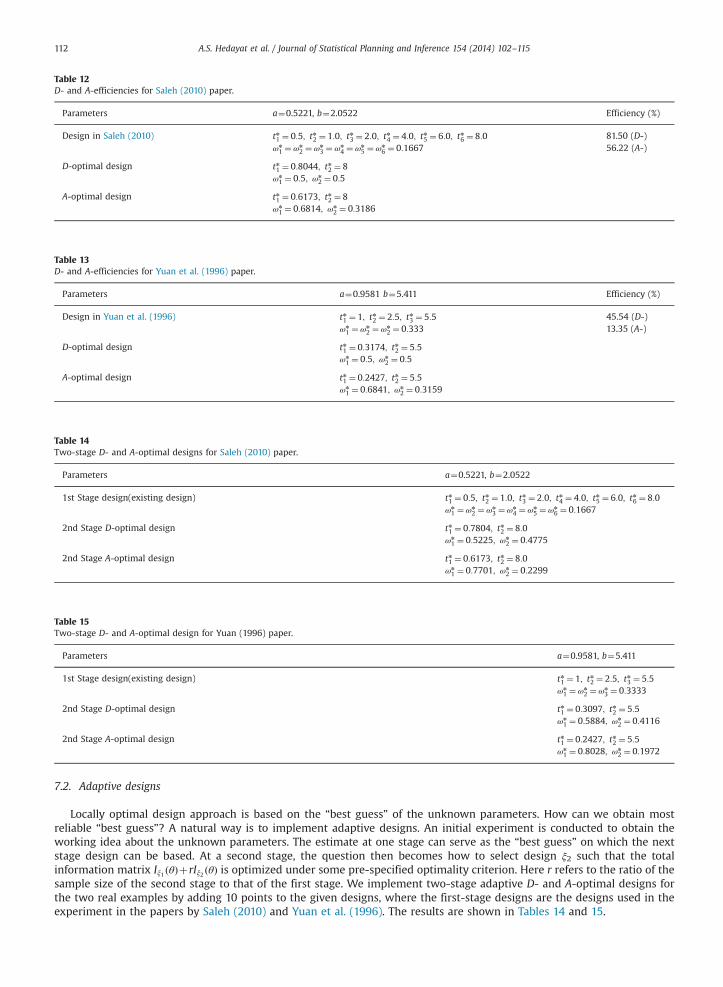
Table 12D- and A-efficiencies for Saleh (2010) paper.

Parameters a¼0.5221, b¼2.0522 Efficiency (%)

Design in Saleh (2010) tn1 ¼ 0:5; tn2 ¼ 1:0; tn3 ¼ 2:0; tn4 ¼ 4:0; tn5 ¼ 6:0; tn6 ¼ 8:0 81.50 (D-)ωn

1 ¼ωn

2 ¼ωn

3 ¼ωn

4 ¼ωn5 ¼ωn

6 ¼ 0:1667 56.22 (A-)

D-optimal design tn1 ¼ 0:8044; tn2 ¼ 8ωn

1 ¼ 0:5; ωn

2 ¼ 0:5

A-optimal design tn1 ¼ 0:6173; tn2 ¼ 8ωn

1 ¼ 0:6814; ωn

2 ¼ 0:3186

Table 13D- and A-efficiencies for Yuan et al. (1996) paper.

Parameters a¼0.9581 b¼5.411 Efficiency (%)

Design in Yuan et al. (1996) tn1 ¼ 1; tn2 ¼ 2:5; tn3 ¼ 5:5 45.54 (D-)ωn1 ¼ωn

2 ¼ωn2 ¼ 0:333 13.35 (A-)

D-optimal design tn1 ¼ 0:3174; tn2 ¼ 5:5ωn

1 ¼ 0:5; ωn

2 ¼ 0:5

A-optimal design tn1 ¼ 0:2427; tn2 ¼ 5:5ωn

1 ¼ 0:6841; ωn

2 ¼ 0:3159

Table 14Two-stage D- and A-optimal designs for Saleh (2010) paper.

Parameters a¼0.5221, b¼2.0522

1st Stage design(existing design) tn1 ¼ 0:5; tn2 ¼ 1:0; tn3 ¼ 2:0; tn4 ¼ 4:0; tn5 ¼ 6:0; tn6 ¼ 8:0ωn1 ¼ωn

2 ¼ωn3 ¼ωn

4 ¼ωn5 ¼ωn

6 ¼ 0:1667

2nd Stage D-optimal design tn1 ¼ 0:7804; tn2 ¼ 8:0ωn

1 ¼ 0:5225; ωn

2 ¼ 0:4775

2nd Stage A-optimal design tn1 ¼ 0:6173; tn2 ¼ 8:0ωn

1 ¼ 0:7701; ωn

2 ¼ 0:2299

Table 15Two-stage D- and A-optimal design for Yuan (1996) paper.

Parameters a¼0.9581, b¼5.411

1st Stage design(existing design) tn1 ¼ 1; tn2 ¼ 2:5; tn3 ¼ 5:5ωn

1 ¼ωn

2 ¼ωn

3 ¼ 0:3333

2nd Stage D-optimal design tn1 ¼ 0:3097; tn2 ¼ 5:5ωn

1 ¼ 0:5884; ωn

2 ¼ 0:4116

2nd Stage A-optimal design tn1 ¼ 0:2427; tn2 ¼ 5:5ωn1 ¼ 0:8028; ωn

2 ¼ 0:1972


7.2. Adaptive designs

Locally optimal design approach is based on the “best guess” of the unknown parameters. How can we obtain mostreliable “best guess”? A natural way is to implement adaptive designs. An initial experiment is conducted to obtain theworking idea about the unknown parameters. The estimate at one stage can serve as the “best guess” on which the nextstage design can be based. At a second stage, the question then becomes how to select design ξ2 such that the totalinformation matrix Iξ1 ðθÞþrIξ2 ðθÞ is optimized under some pre-specified optimality criterion. Here r refers to the ratio of thesample size of the second stage to that of the first stage. We implement two-stage adaptive D- and A-optimal designs forthe two real examples by adding 10 points to the given designs, where the first-stage designs are the designs used in theexperiment in the papers by Saleh (2010) and Yuan et al. (1996). The results are shown in Tables 14 and 15.

Fig. 1. Distribution of D- and A-efficiencies. (a) D-efficiency: Saleh (2010), (b) A-efficiency: Saleh (2010), (c) D-efficiency: Yuan et al. (1996), (d) A-efficiency:Yuan et al. (1996).


7.3. Simulation study

Clearly the derived adaptive designs depend on the estimated parameter values from the first stage design. This impliesthat the adaptive designs are not uniquely determined since the estimated parameter values are random variables.A simulation study is conducted to evaluate the performance of the derived adaptive designs. We use the designs in Saleh(2010) and Yuan et al. (1996) as the first stage designs. We also use the estimated parameters in Saleh (2010) and Yuan et al.(1996) as the true parameters values. The simulation study consists of three steps: (i) drawing a random variable from themultivariable normal distribution based on the estimation from the first stage design; (ii) deriving the adaptive optimaldesign based on the drawn parameter values; and (iii) evaluating the efficiency of the derived adaptive design using a localoptimal design as a benchmark. We repeated the process 1000 times and we obtained the distribution of efficiency.The mean and the standard deviation of D- and A-efficiencies are reported respectively for both examples: they are 0.86(0.08)and 0.54(0.02) for Saleh (2010); 0.88(0.07) and 0.38(0.01) for Yuan et al. (1996). The histograms of the efficiencies arepresented in Fig. 1.

Another interesting question is, what is the relative efficiency if we use the existing design in the paper at both the firstand the second stages compared to the situation that if we use the adaptive optimal design at the second stage? We found,after running the similar simulation study, the relative D-efficiencies for Saleh and Yuan's paper are 0.78(0.17) and 0.35(0.10)and the relative A-efficiencies are 0.30(0.07) and 0.14(0.01). Both examples show that using adaptive designs at the secondstage is better than using the existing designs at both stages.

8. Discussion

Searching for optimal designs is important and also complicated. Knowing the upper-bound of the number of supportpoints can greatly simplify the search process, numerically or analytically. We have a complete answer for Klimpel's flotation


recovery model. However, we only have partial answer for 2-parameter chemical kinetic model as well as compartmentmodels. Extensive numerical studies suggest that optimal designs can be based on saturated designs. How to prove thisconclusion remains an open problem.

Optimal designs for compartment models are less sensitive, while both Klimpel's flotation recovery model and2-parameter chemical kinetic model suffer significant efficiency loss when parameters are moderately deviated from theirtrue values. Bayesian or minimax optimal designs could be a remedy for this problem.

Adaptive designs are promising since with any existing design at the first stage and initial information about parametervalues, adaptive optimal designs can be derived for the second stage for certain optimality criterion. Our simulation alsoshows that adaptive designs are comparable to local optimal designs in some cases. Given the first stage existing designs,using adaptive designs at the second stage is also efficient than using the existing design at the second stage.

Acknowledgments

Especially, we want to thank Professor Bikas Sinha from Indian Statistical Institute for his generous help on revising themanuscript.

Appendix

Lemma 1. The following two systems are ECT-systems:

(1)
T1 ¼ f1; x; x2; x2 ln x; x2ðln xÞ2g is an ECT-system with W1ðu0;u1;…;ukÞðxÞ40. (2) T2 ¼ f1; x; x2; x2 ln x; x ln xg is an ECT-system with W2ðu0;u1;…;ukÞðxÞ40.
Proof. We give a detailed proof for T1. Similar proof for T2 can be derived similarly. It can be shown that

W1ðu0ÞðxÞ ¼ 140,W1ðu0;u1ÞðxÞ ¼ 140,

W1 u0;u1;u2ð Þ xð Þ ¼1 0 0x 1 0x2 2x 2

��¼ 240;

W1 u0;u1;u2;u3ð Þ xð Þ ¼

1 0 0 0x 1 0 0x2 2x 2 0x2 ln x 2x ln xþx 2 ln xþ3 2

x

��

��¼ 4

x40;

and

W1 u0;u1;u2;u3;u4ð Þ xð Þ

¼

1 0 0 0 0x 1 0 0 0x2 2x 2 0 0x2 ln x 2x ln xþx 2 ln xþ3 2

x � 2x2

x2ðln xÞ2 2xðln xÞ2þ2x ln x 2ðln xÞ2þ6 ln xþ2 4x ln xþ6

x � 4x2 ln x� 2

x2

��

��¼ 16

x340:

Therefore, f1; x; x2; x2 ln x; x2ðln xÞ2g is an ECT-system, which is also a T-system. □

Lemma 2. g1ðtÞ defined in (5.4) is a linear combination of T-systems and has at most 5 roots.

Proof. Let g1ðtÞ ¼ a1t2eðλ2 � λ1Þtþb1teðλ2 � λ1Þtþc1eðλ2 � λ1Þtþa2t2eðλ1 � λ2Þtþb2teðλ1 � λ2Þtþc2eðλ1 � λ2Þt , which can be re-written asg1ðtÞ ¼ ð1=eðλ2 � λ1ÞtÞ½e2ðλ2 � λ1Þtða1t2þb1tþc1Þþa2t2þb2tþc2�.To find out the number of roots for g1ðtÞ ¼ 0, consider ~g2 ðtÞ ¼ ½e2ðλ2 � λ1Þtða1t2þb1tþc1Þþa2t2þb2tþc2� ¼ 0.Since d3 ~g2 ðtÞ=dt3 ¼ e2ðλ2 � λ1Þtða01t2þb01tþc01Þ, has at most 2 roots, g1ðtÞ has at most 5 roots. Therefore, it is a T-system. □


References

Bernshtein, S.N., 1937. The extremal properties of polynomials and best approximation of continuous functions of a real variable. Moscow-Leningrad(in Russian).

Biedermann, S., Dette, H., Zhu, W., 2006. Optimal designs for dose–response models with restricted design spaces. J. Amer. Statist. Assoc. 101 (474), 747–759.Boroujerdi, M., 2001. In: Pharmacokinetics: Principles and Applications. McGraw-Hill, New York.Chebyshev, P.L., 1859. Questions on smallest quantities connected with the approximate representation of functions. In: Collected Works, vol. 2, Moscow-

Leningrad, pp. 151–238 (in Russian).Ding, A.A., Wu, H., 2000. A comparison study of models and fitting procedures for biphasic viral dynamics in HIV-1 infected patients treated with antiviral

therapies. Biometrics 56 (1), 293–300.Fang, X., Hedayat, A.S., 2008. Locally D-optimal designs based on a class of composed models resulted from blending Emax and one-compartment models.

Ann. Statist. 36, 428–444.Gieschke, R., Steimer, J.L., 2000. Pharmacometrics: modelling and simulation tools to improve decision making in clinical drug development. Eur. J. Drug

Metabolism Pharmacokinetics 25 (1), 49–58.Godfrey, K., 1983. In: Compartmental Models and Their Application. Academic Press, London.Han, C., Chaloner, K., 2003. D- and C-optimal designs for exponential regression models used in viral dynamics and other applications. J. Statist. Plann.

Inference 115, 585–601.Hartman, P., 1964. Ordinary Differential Equations. Wiley, New York.Hedayat, A.S., Yan, B., Pezzuto, J.M., 1997. Optimum designs for fitting dose–response curves based on raw optical density data. J. Amer. Statist. Assoc. 92,

1132–1140.Jacquez, J.A., 1985. In: Compartmental Analysis in Biology and Medicine, 2nd ed. The University of Michigan Press, Ann Arbor.Karlin, S., Studden, W.J., 1966. Tchebycheff Systems: With Applications in Analysis and Statistics. Pure and Applied Mathematics XV. Wiley, New York.Kiefer, J., 1974. General equivalence theory for optimum designs (approximate theory). Ann. Statist. 5, 849–879.Li, G., Majumdar, D., 2008. D-optimal design for logistic models with three and four parameters. J. Statist. Plann. Inference 138, 1950–1959.Meibohm, B., Derendorf, H., 2002. Pharmacokinetic/pharmacodynamic studies in drug product development. J. Pharmaceutical Sci. 91 (1), 18–31.Parekh, B.K., Miller, J.D., 1999. Advances in Flotation Technology. Society for Mining Metallurgy and Exploration, Denver.Saleh, A.M., 2010. A study on the performance of second order models and two phase models in iron ore flotation. Physicochemical Probl. Mineral Process.

44, 215–230.Silvey, S.D., 1980. Optimal Design: An Introduction to the Theory for Parameter Estimation. Chapman & Hall, London.White, L., 1973. An extension of the general equivalence theorem to nonlinear models. Biometrika 60, 345–348.Yang, M., Biedermann, S., Tang, E., 2013. On optimal designs for nonlinear models: a general and efficient algorithm. J. Am. Statist. Assoc. 108, 1411–1420.Yang, M., Stufken, J., 2009. Support points of locally optimal designs for nonlinear models with two parameters. Ann. Statist. 37, 518–541.Yang, M., 2010. On the de la Garza phenomenon. Ann. Statist. 38, 2499–2524.Yuan, X.M., Påilsson, B.I., Forssberg, K.S.E., 1996. Statistical interpretation of flotation kinetics for a complex sulphide ore. Minerals Eng. 9 (4), 429–442.

http://refhub.elsevier.com/S0378-3758(14)00079-2/sbref2






























optimal designs for some selected nonlinear...

Documents